IPN Progress Report 42-154 August 15, 2003

Control Systems of the Large Millimeter TelescopeW. Gawronski1 and K. Souccar2

This article presents the analysis results (in terms of settling time, bandwidth,and servo error in wind disturbances) of four control systems designed for the LargeMillimeter Telescope (LMT). The first system, called the PP system, consists ofthe proportional-and-integral (PI) controllers in the rate and position loops andis widely used in the antenna and radio telescope industry. The analysis showsthat the PP control system performance is remarkably good when compared tosimilar control systems applied to typical antennas. This performance is achievedbecause the LMT structure is exceptionally rigid, but the performance does notmeet the stringent pointing requirements of the LMT. The second system, calledthe PL system, consists of the PI controller in the rate loop and the linear-quadratic-Gaussian (LQG) controller in the position loop. It is implemented at the NASADeep Space Network antennas, and its pointing precision is twice as good as thePP control system. The third system, called the LP system, consists of the LQGcontroller in the rate loop and the proportional-integral-derivative (PID) controllerin the position loop. It has not been implemented yet at known antennas or radiotelescopes, but the analysis shows that its pointing accuracy is ten times betterthan the PP control system. The fourth system, called the LL system, consists ofthe LQG controller in the rate loop and in the position loop. It is the best of thefour (its precision is 250 times better than the PP system); thus, it is worth furtherinvestigation and verification of implementation challenges for telescopes with highpointing requirements.

I. Introduction

The Large Millimeter Telescope (LMT) Project is a joint effort of the University of Massachusettsat Amherst and the Instituto Nacional de Astrofisica, Optica, y Electronica (INAOE) in Mexico. TheLMT is a 50-m-diameter millimeter-wave radio telescope (see Fig. 1) designed for principal operation atwavelengths between 1 mm and 4 mm. The telescope is being built atop Sierra Negra (4640 m), a volcanicpeak in the state of Puebla, Mexico. Site construction and fabrication of most of the major antenna partsis under way, with telescope construction expected to be complete in 2005.

1 Communications Ground Systems Sections.

2 LMT Project, Astronomy Department, University of Massachusetts, Amherst.

The research described in this publication was carried out by the Jet Propulsion Laboratory, California Institute ofTechnology, and was partially funded by the National Science Foundation and the Advance Research Project Agency,Sensor Technology Office, issued by DARPA/CMO.

1

MAIN REFLECTOR

SUBREFLECTOR

AZIMUTH WHEELS

BACK STRUCTURE

ELEVATION GEAR

ELEVATION AXIS

RECEIVER CABIN

ALIDADE

FOUNDATION

Fig. 1. A drawing of the Large Millimeter Telescope. The whole structure rotates with respect to thevertical axis (azimuth) on the azimuth wheels, and the dish rotates with respect to the horizontal(elevation) axis.

The LMT will be a significant step forward in antenna design since, in order to reach its pointingand surface accuracy specifications, it must outperform every other telescope in its frequency range.The largest existing telescope with surface error superior to the LMT is the 15-m James Clerk MaxwellTelescope, located at the summit of Mauna Kea (4092 m) in Hawaii, and there is no telescope of any sizethat reaches the LMT pointing requirements. The antenna designer expects that this system will pointthe telescope to its specified accuracy of 1 arcsec under conditions of low winds and stable temperatures.However, under the maximum operating wind conditions, the pointing will degrade to a few arcseconds(rms). The pointing challenges and their solutions are discussed in [1] and [8].

It is known that the linear-quadratic-Gaussian (LQG) controllers guarantee wide bandwidth and goodwind-disturbance rejection properties [2]; thus, they are used for antennas with stringent pointing re-quirements in the presence of wind disturbances. For antennas and radio telescopes, the LQG controlsystems can be implemented in two different ways: at the telescope rate loop or at the position loop.This article analyzes and compares the performances of the LQG controllers at these two locations. Theanalysis is augmented with the performance of the proportional-and-integral (PI) controller. The latteranalysis is necessary not only for comparison purposes (the PI controller is a standard antenna industryfeature), but also because the implementation of the LQG controller requires preliminary installationof PI controllers in both rate and position loops. The implementation of the LQG algorithm needs an

2

accurate telescope model, and it can be obtained from the field test of the telescope. Thus, a telescopewill be operational before the LQG controller implementation.

Why do we need an accurate rate-loop model? It can be explained as follows. The performanceof a controller improves with the gain increase. However, high gains excite structural vibrations. Fora PI controller, structural vibrations cannot easily be controlled since the structural deformations arenot directly measured by encoders. But an LQG controller uses a Kalman filter to estimate telescopevibrations, overcoming the difficulty of direct measurement. The Kalman filter consists of a telescopeanalytical model that needs to be accurate to produce an accurate estimate of the telescope structuraldynamics.

The control system of the LMT consists of rate and position loops, as shown in Fig. 2. Four controlsystems will be analyzed. They have the following structure:

(1) PP control system, with a PI controller in the position loop and a PI controller in therate loop

(2) PL control system, where the PI controller is in the rate loop and the LQG controller isin the position loop

(3) LP control system, where the LQG controller is in the rate loop and the PID (proportional-integral-derivative) controller is in the position loop

(4) LL control system, where the LQG controller is in the rate loop and the LQG controlleris in the position loop

The configurations of the control systems are presented in Table 1. The PP control system is a typicaltelescope control system configuration. The PL case is the configuration of the NASA Deep SpaceNetwork (DSN) antenna control system, and it was implemented at the 34-meter antennas in Goldstone,California. The LQG controller has been considered by MAN Technologie [1,8]. The LP and LL controlsystems have not been implemented yet.

COMMANDRATE

COMMANDTORQUE

POSITION

RATE

POSITION

POSITION-LOOPCONTROLLER (PC)

RATE-LOOPCONTROLLER (RC)

TELESCOPE ANDDRIVES

Fig. 2. Four control systems of the LMT: (1) the PP control system, where RC = PI and PC = PI, (2) the PL controlsystem, where RC = PI and PC = LQG, (3) the LP control system, where RC = LQG and PC = PID, and (4) the LL controlsystem, where RC = LQG and PC = LQG.

Table 1. Configurations of the control systemsof the Large Millimeter Telescope.

LMT control Rate-loop Position-loopsystem controller controller

PP PI PI

PL PI LQG

LP LQG PID

LL LQG LQG

3

This article presents the performance analysis (in terms of bandwidth, step responses, and wind-disturbance rejection properties) of the four control systems as applied to the LMT. This analysis willhelp to evaluate and select the control system not only for the LMT, but also for other antennas andradio telescopes of a similar design.

II. The PP Control System

The PP control system consists of a PI controller in the position loop and a PI controller in the rateloop. Its Simulink model is shown in Fig. 3(a) and the rate-loop subsystem in Fig. 3(b). The controller isshown in Fig. 3(c), with kf = 0. In this design, the position-loop PI controller is complemented with thefeedforward (FF) loop to improve the tracking properties, especially at high rates, and with a commandpreprocessor (CPP) to avoid large overshoots during target acquisition and limit cycling during slewing.

A. The Rate-Loop Model

The rate-loop model is shown in Fig. 3(b). It consists of the finite-element model (FEM) of thetelescope structure (labeled “Discrete Time FEM”), which includes the drives and the azimuth (AZ) andelevation (EL) rate-loop controllers. It is a discrete-time (digital) control system with a 0.001-s samplingtime. The proportional-and-integral gains of the azimuth controller are 300; for the elevation controller,the proportional gain is also 300, and the integral gain is 400. The bandwidth of the rate-loop transferfunction is 1.0 Hz, both in azimuth and in elevation.

B. Command Preprocessor

Before the position loop is presented, we consider the rate and acceleration limits imposed at the drives.The acceleration limits prevent motors from overheating (the motor current is proportional to telescopeacceleration). During tracking, the telescope motion is within the rate and acceleration limits. However,during slewing, the large position-offset commands exceed the acceleration limit or both the accelerationand rate limits. When limits are exceeded, the telescope dynamics are no longer linear, and the telescopebecomes unstable, which is observed in the form of limit cycling (periodic motion of constant magnitudeand of low frequency). Since the limit cycling is caused by commands that exceed the acceleration andrate limits, one easily can avoid the instability by properly shaping commands such that the limits arenot exceeded.

The command preprocessor modifies the telescope commands such that they remain unaltered if theydo not exceed the rate and acceleration limits, and it processes the command to the maximum accelerationand rate limits if the limits are exceeded by the command. The block diagram of the CPP is shownin Fig. 4. The CPP algorithm represents an integrator, rate and acceleration limits, a variable-gaincontroller, and a feedforward gain. Its input is a command r, and its output is the modified command rf .

The variable gain k depends on the CPP tracking error e:

k(e) = ko + kve−β|e|

where e = r− rf . For the LMT, we selected the following parameters: ko = 0.3, kv = 1.0, and β = 20 forboth azimuth and elevation. The plot of the gain k versus the error e is shown in Fig. 5. For more onthe CPP, see [3].

Figure 6 shows how the CPP transforms a 10-deg step command for the LMT. The transformed stepcommand shows the initial rise at the maximal acceleration, followed by maximal rate slope, and decel-eration slowdown (which is smaller than the maximal deceleration in order to avoid excessive telescopeshaking). By processing the commands, the CPP allows for smooth telescope responses to step offsetsand eliminates telescope limit cycling during slewing (see Section II.D on the position-loop analysis).

4

AccelerationLimit

AZ CommandAZ CPP

EL Command

AZ PC

AZ FF

EL FF

EL PC

Rate Loop

AZ Position Feedback

EL Position Feedback

AZ Rate

EL RateRateLimit

RateLimit

AZ Rate Input

AZ Encoder

EL Rate Input

EL Encoder

AZ Wind

EL Wind

AZ Encoder

EL Encoder

Windaz

Windel

AccelerationLimit

raz

yaz

yel

relCPP EL

+

+

+

+

(a)

4

(b) AZ Rate Feedback

EL Rate Feedback

AZ RateController

AZ Encoder

EL Encoder

EL RateController

AZ Wind

EL Rate Input

AZ Rate Input

Discrete TimeFEM

3

2

1 1

2

EL Wind

Fig. 3. The Simulink model of (a) the position loop, (b) the rate loop system, and (c) the controller(for kf = 0 it is a PI controller; for kf ≠ 0 it is an LQG controller).

5

Tz − 1

1

2y

r

ki

kf

kp

+

−

+

u

(c)

Estimator

Integrator

−+

−+

Fig. 3 (contd).

1

∫

r

r

r

rfe u

d

dt

VARIABLEGAIN

RATELIMIT

RIGIDTELESCOPE

FEED-FORWARD

ACCELERATIONLIMIT

+

+k (e )+−

Fig. 4. The CPP block diagram.

1.5

1.0

0.5

0.0

CP

P G

AIN

k

10−4 10−3 10−2 10−1 100 101

ERROR e, deg

Fig. 5. CPP gain k versus CPP error e.

6

1210

0CP

P R

ES

PO

NS

E, d

eg0

TIME, s

Fig. 6. CPP response rf to 10-deg step command r.

5 10 15 20 25 30

2

4

6

8

rf

r

C. Feedforward Loop

The feedforward loop is added to improve tracking accuracy, especially at high rates. The feedforwardloop differentiates the command and forwards it to the rate-loop input [see Fig. 3(a)]. The derivative is theinversion of the rate-loop transfer function. In this way, we obtain the open-loop transfer function fromthe command to the encoder, approximately equal to 1. Indeed, the magnitude of the rate-loop transferfunction Gr is shown in Fig. 7. It can be approximated (up to 1 Hz) with an integrator (Grapprox = 1/s),which is shown in the same figure (short-dashed line). The feedforward transfer function is a derivative(Gff (s) = s) shown in Fig. 7 (long-dashed line), so that the overall open-loop transfer function is a seriesconnection of the feedforward and the rate loop Go(s) = Gr(s)Gff (s), which is approximately equal to 1up to a frequency of 1 Hz. In this way, the transfer function of the system is equal to 1 (up to 1 Hz)without applying the position feedback. The position feedback is added to compensate disturbances andsystem imperfections.

D. Position Loop

The position-loop model is shown in Fig. 3. It consists of the rate-loop model, PI and feedforwardcontrollers in azimuth and elevation, command preprocessors in azimuth and elevation, and rate andacceleration limiters in azimuth and elevation. The telescope rate limit is 1.0 deg/s, and the accelerationlimit is 0.5 deg/s2, both in azimuth and elevation. The PI controller gains were selected to minimizesettling time and servo error in wind gusts. They also guarantee zero steady-state error for constant ratetracking. The proportional gain is 3.0, and the integral gain is 1.0.

The position-loop transfer functions for azimuth and elevation are shown in Fig. 8. It follows from thisfigure that the azimuth bandwidth is 1.2 Hz, while the elevation bandwidth is 1.8 Hz (the bandwidth is thefrequency for which the magnitude of the transfer function falls below level 0.7). Note that the position-loop bandwidth is higher than the rate-loop bandwidth, both in azimuth and elevation. Note also thatthe elevation-axis bandwidth is higher than the azimuth-axis bandwidth, mainly because the elevationtransfer function has only a few resonances and the resonances are well damped. Azimuth bandwidth islower since the controller gains will be low in order to prevent excitation of multiple resonances.

In order to evaluate settling time, we simulated the step responses for small (0.01-deg) and large(3.0-deg) steps. The azimuth step responses are shown in Fig. 9 for the telescope with and without aCPP. From the plots, one can see that there is no overshoot when a CPP was implemented, and that thesettling time is 3.0 s (small steps) in azimuth and elevation. Without a CPP, we observe overshoots forsmall steps and a settling time of 4.5 s in azimuth and elevation. For larger steps (e.g., when slewing),the telescope becomes unstable, showing limit cycling (see Fig. 9).

The wind-gust time history was obtained from the wind spectrum (see [4]). The plot of the servoerrors in azimuth and elevation is shown in Fig. 10 (in black).

7

10−4

MA

GN

ITU

DE

10−2 10−1 100 102

FREQUENCY, Hz

Fig. 7. The feedforward action illustrated by the magni-tudes of the transfer functions (Gr is the rate-loop transferfunction, Grapprox is the rate-loop transfer functionapproximation, Gff is the feedforward loop transferfunction, and Go = Gff Gr is the transfer function of theseries connection of feedforward and rate loops).

101

10−3

10−2

10−1

100

101

102

103

Grapprox

Gr

Gff

Go = Gff Gr

EL

−300

PH

AS

E, d

eg

10−2 10−1 101 102

FREQUENCY, Hz

Fig. 8. Position-loop transfer function in azimuth (solid line) and elevation(dashed line): (a) magnitude and (b) phase.

100

AZ

−200

−100

0

100

EL

10−2

MA

GN

ITU

DE

10−2 10−1 101 102

FREQUENCY, Hz

100

10−1

100

101

AZ1.0

0.7 AZ BANDWIDTH

EL BANDWIDTH

(a)

(b)

8

−1

TIME, s

Fig. 9. Telescope responses in azimuth, with the CPP (solid line) and with-out the CPP (dashed line) to a: (a) 0.01-deg step and (b) 1-deg step.

0

1

2

3

0.002

AZ

ST

EP

RE

SP

ON

SE

,de

g

0

TIME, s

WITHOUT CPP

WITH CPP

(a)

0.000

0.004

0.006

0.008

0.010

0.012

2 4 6 8 10 12 14 16 18 20

AZ

ST

EP

RE

SP

ON

SE

,de

g

0 1 2 3 4 5 6 7 8 9 10

WITHOUT CPP

WITH CPP

(b)

−5

−4

−3

−2

−1

0

1

2

3

4

5

EL

SE

RV

O E

RR

OR

, mde

g

−5 −4 −3 −2 −1 0 1 2 3 4 5

AZ SERVO ERROR, mdeg

Fig. 10. Telescope servo error in 12-m/s wind gusts:with the PP control system (black), with the PL controlsystem (gray), with the LP control system (white), andwith the LL control system (zoomed insert).

−0.02

0

−0.02 0 0.02

LLPP

PL

LP

0.02

9

The PP control system analysis showed also that the LMT is a sturdy structure. Its fundamentalfrequency is 1.7 Hz (for a typical radio telescope, it will be 1.3 Hz, as shown in Fig. 11). The rigidstructure allowed for high gains of PI controllers (3.0 proportional gain and 1.0 integral gain). Forcomparison, the NASA Deep Space Network antenna fundamental frequency is 1.8 Hz (although, as asmaller structure, it should have a higher frequency), and allows for 0.5 proportional gain and 0.1 integralgain (3.0 proportional gain and 1.0 integral gain destabilize it). Higher gains mean wider bandwidth(over 1 Hz), faster response (a settling time of 3 s), and improved wind-disturbance rejection properties.In conclusion, the LMT performs better than could be expected for the PP-type of control system.

III. The PL Control System

The PL control system consists of the LQG controller in the position loop and the PI controller in therate loop.

A. Rate Loop

In this case, the rate-loop model of the telescope is as shown in Fig. 3(a). It consists of the structureand drive model and the azimuth and elevation rate-loop controllers (PI type). The PI gains of the ratecontrollers were given in Section II.A.

B. Position Loop

The position loop is presented in Fig. 3, where the PI controllers are replaced with the LQG controllersas in Fig. 3(c). It consists of the same rate-loop model as in the PP control system, the LQG controllerwith feedforward loop, the command preprocessor, and rate and acceleration limits. The CPP parametersare as follows: kv = 6, ko = 0.6, and β = 20 for azimuth and elevation.

The LQG controller structure is shown in Fig. 12. The controller includes the estimator, which is ananalytical model of the telescope. The estimator is driven by the same input (uc) as the telescope, but

1 2 4 6 8 10 20 40 60 80 100

d, ANTENNA DIAMETER, m

0.8

1

2

4

6

8

10

20

d = 50 m(LMT DIAMETER)

f = 1.7 Hz(for LMT)

f = 1.3 Hz(for a typical antenna)

f = 20.0 d −0.7f, A

NT

EN

NA

LO

WE

ST

FR

EQ

UE

NC

Y, H

z

Fig. 11. Antenna fundamental frequency versus antenna diameter.This plot is based on data from the Lowest Servo Resonant Fre-quency Chart by the Aerospace Corporation.

10

Fig. 12. The LQG controller structure.

ESTIMATOR

ki

er

−

+

y−

+

ei

kp

kfxf

xest

ke

+

++

uc

ε

uc

∫

also by the estimation error ε (the difference between the actual rate y and the estimated rate yest). Theerror is amplified with the estimator gain ke to correct for transient dynamics. The estimator outputs arethe estimated telescope states that consist of the telescope rate and the telescope flexible deformations xf .The latter are the missing vibration measurements, which allow for suppression of the telescope vibrations.The gains of the rate-loop LQG controller were obtained from the LQG design procedure (see [5–7,9]).

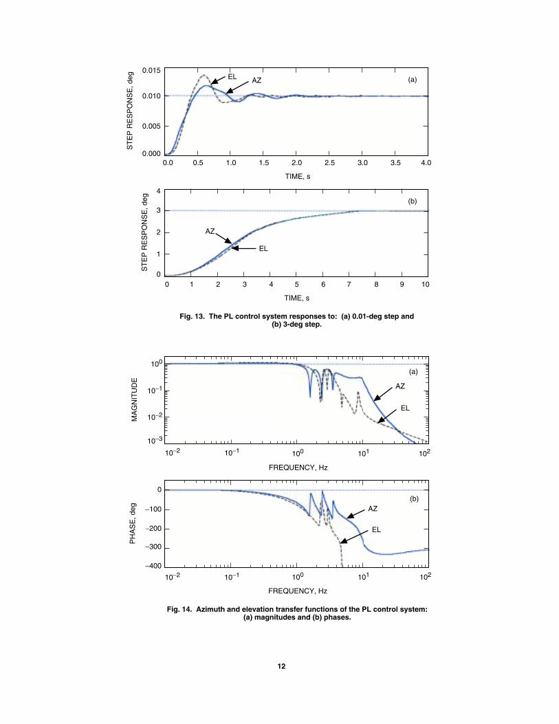
We evaluated the performance of the PL control system using settling time, bandwidth, and servoerror in wind gusts. The step responses for small (0.01-deg) and large (3-deg) steps are shown in Fig. 13.Figure 13(a) shows 1.6-s settling time in azimuth, 1.2-s settling time in elevation, 18 percent overshootin azimuth, and 35 percent overshoot in elevation. The position-loop transfer functions for azimuth andelevation are shown in Fig. 14. They show a wide bandwidth of 1.3 Hz in azimuth and 1.5 Hz in elevation.

The wind-gust simulations show 0.15-mdeg rms servo error in azimuth and 0.74-mdeg rms servo errorin elevation (see the servo error in wind gust plotted in Fig. 10 in gray). These numbers are comparedwith the PP control system (0.35 mdeg in azimuth and 1.4 mdeg in elevation). This means that the LQGcontroller improves the servo error in wind over the PID controller by a factor of 2.3 in azimuth and afactor of 1.9 in elevation.

The results obtained on the LQG position controller are promising. The telescope had a settling timeof 1.6 s, bandwidth of 1.3 Hz, and wind servo error of 0.76 mdeg—or 2 times smaller than that of the PPcontrol system.

IV. The LP Control System

The LP control system consists of the PID (proportional-integral-derivative) controller in the positionloop and the LQG controller in the rate loop. Its Simulink model is shown in Fig. 3(a) and the rate-loopsubsystem in Fig. 3(b).

A. Rate Loop

The Simulink model of the open-loop telescope is as shown in Fig. 3(b), with the rate feedbackremoved. The open-loop model is scaled to obtain a maximal rate of 1 deg/s for a 10-V command (a

11

EL

0

ST

EP

RE

SP

ON

SE

, deg

0

TIME, s

Fig. 13. The PL control system responses to: (a) 0.01-deg step and(b) 3-deg step.

AZ

EL

0.000

ST

EP

RE

SP

ON

SE

, deg

0.0

TIME, s

AZ

(b)

1 2 3 4 5 6 7 8 9 10

1

2

3

4

0.5 1.0 1.5 2.0 2.5 3.0 3.5 4.0

0.005

0.010

0.015(a)

EL

−300

PH

AS

E, d

eg

10−2 10−1 101 102

FREQUENCY, Hz

Fig. 14. Azimuth and elevation transfer functions of the PL control system:(a) magnitudes and (b) phases.

100

AZ

−200

−100

0

EL

10−3

MA

GN

ITU

DE

10−2 10−1 101 102

FREQUENCY, Hz

100

10−2

10−1

100

AZ

(a)

(b)

−400

12

standard input to motor drives). For this open-loop model, we designed an LQG controller and evaluatedthe performance of the rate-loop LQG controller using its step responses and transfer functions of theazimuth and elevation rate-loop; the settling time is 0.2 s in azimuth and elevation, and the bandwidthis 1.6 Hz and 1.8 Hz in azimuth and elevation, respectively.

B. Position Loop

The position loop is as shown in Fig. 3, but the azimuth and elevation rate controller are now of theLQG type. Besides the rate loop, the control system consists of the PID controller with a feedforwardloop, the command preprocessor, and rate and acceleration limiters. The feedforward loop forwards thecommand rate to the rate-loop input. The following PID gains were selected: proportional gain, 10;integral gain, 6; and derivative gain, 5, for both azimuth and elevation. The CPP parameters are asfollows: kv = 6, ko = 0.93, and β = 30, for azimuth and elevation.

The position-loop performance was evaluated using step responses, bandwidth, steady-state errors dueto rate offsets, and servo errors in wind gusts. The step responses for small (0.01-deg) and large (3-deg)steps are shown in Fig. 15, showing 0.6-s settling time and no overshoot for both azimuth and elevation.

The position-loop transfer functions for azimuth and elevation are shown in Fig. 16. They show a widebandwidth of 200 Hz in azimuth and 20 Hz in elevation. The steady-state error due to rate offsets is zero.

The wind-gust simulations for a 12-m/s wind are plotted in Fig. 10 (white). The figure shows0.012-mdeg rms servo error in azimuth and 0.150-mdeg rms servo error in elevation. These small numbersshow that, as compared with the PP control system, the LQG controller in the rate loop improves theservo error in wind by a factor of 30 in azimuth and a factor of 10 in elevation.

The results obtained on the LQG rate controller are very promising. The telescope performanceexceeds the expectation, since its settling time is 0.6 s, the bandwidth is 10 Hz, and wind servo error is0.15 mdeg—or 10 times smaller than with the PID controller.

V. The LL Control System

Finally, we designed the telescope control system with the LQG controller in the rate and positionloops. This is also a novel configuration in the antenna industry.

A. Rate Loop

The rate loop is the same as for the LP control system.

B. Position Loop

For the given rate loop, the position-loop controller was designed to minimize the servo error in thewind gusts. The position-loop characteristics are plotted in Figs. 17 and 18. From Fig. 17, it follows thatthe system settling time is 0.5 s, and there is no overshoot in either azimuth or elevation. From Fig. 18,one can find that the bandwidth is 20 Hz in azimuth and 40 Hz in elevation. Finally, the wind-gustsimulations for a 12-m/s wind are plotted in the zoomed insert in Fig. 10. The figure shows 0.0012-mdegrms servo error in azimuth and 0.0057-mdeg rms servo error in elevation, which give a total rms errorof 0.0058 mdeg. It is 250 times smaller than the error of the PP control system. Thus, the LL controlsystem performance is the best of all the systems presented, although the system is the most complicatedand will require careful tuning of both rate- and position-loop LQG controllers in order to obtain thepredicted performance.

13

0

ST

EP

RE

SP

ON

SE

, deg

0

TIME, s

Fig. 15. The LP control system position-loop response to:(a) 0.01-deg step and (b) 3-deg step.

EL

0.000

ST

EP

RE

SP

ON

SE

, deg

0.0

TIME, s

AZ

(b)

1 2 3 4 5 6 7 8

1

2

3

4

0.2 0.4 0.6 0.8 1.0 1.2 1.8 2.0

0.004

0.008

0.012

(a)

0.006

0.002

0.010

1.4 1.6

AZ and EL

EL

−135

PH

AS

E, d

eg

10−2 10−1 101 102

FREQUENCY, Hz

Fig. 16. Azimuth and elevation position-loop transfer functions of the LPcontrol system: (a) magnitudes and (b) phases.

100

AZ

−90

−45

0

EL

MA

GN

ITU

DE

10−2 10−1 101 102

FREQUENCY, Hz

100

10−1

100AZ

−180

45

(a)

(b)

14

0

ST

EP

RE

SP

ON

SE

, deg

0

TIME, s

Fig. 17. The LL control system position-loop response to:(a) 0.01-deg step and (b) 3-deg step.

EL

0.000

ST

EP

RE

SP

ON

SE

, deg

0.0

TIME, s

AZ

(b)

1 2 3 4 5 6 7 8

1

2

3

4

0.2 0.4 0.6 0.8 1.0 1.2 1.8 2.0

0.004

0.008

0.012

(a)

0.006

0.002

0.010

1.4 1.6

AZ and EL

EL

−150PH

AS

E, d

eg

10−2 10−1 101 102

FREQUENCY, Hz

Fig. 18. Azimuth and elevation position-loop transfer functions of the LLcontrol system: (a) magnitudes and (b) phases.

100

AZ−100

−50

0

EL

MA

GN

ITU

DE

10−2 10−1 101 102

FREQUENCY, Hz

100

10−2

100

AZ

−200

101

10−1

(a)

(b)

15

VI. Conclusions

This article presented the LMT control systems and evaluated their performances, which are summa-rized in Table 2.

The PP control system is widely used in the antenna and radio telescope industry. The analysis showsthat the LMT structure is exceptionally rigid; thus, the PP control system shows improved pointingaccuracy when compared with similar control systems applied to typical antennas or telescopes. The PLcontrol system is implemented at the NASA Deep Space Network antennas, and its pointing precision inwind is twice as good as that of the PP system. The LP control system has not been implemented yetat known antennas or radio telescopes, and the analysis shows that its pointing accuracy in wind is tentimes better than that of the PP system. This significant reduction was achieved because of the expandedbandwidth of the rate loop. The LL control system also has not been implemented yet at known antennasor radio telescopes. The analysis shows that its pointing accuracy in wind is 250 times better than thatof the PP system. Both the LP and LL control systems are worth further investigation in hope that theirimplementation will meet the stringent pointing requirements.

Finally, some comments on the obtained performance estimates of the telescope are necessary. Theestimates, the best currently available, include some unknown factors. First, the structural model factor:the presented telescope performance is based on the analytical models of the structure and the drives,which do not represent accurate dynamics of the telescope. To improve the accuracy, a model will bederived from the system identification and data collected at the real telescope. Next, the wind disturbancetorques are applied to the drives, while in reality the wind acts on the entire structure, including thedish surface. Finally, the RF beam movement is the ultimate goal of the control, and it is not directlymeasured. Instead, azimuth and elevation encoders are used, which only partially reflect the beamposition. The encoders—although relatively precise—cannot exactly measure the actual beam positiondue to their distant location from the beam focal point, which is the RF beam location.

The performed analysis shows the impact of the location of telescope controllers on the telescope’spointing accuracy and should help to select the most effective system (in terms of cost and precision).

Table 2. Performance of the PP, LP, PL, and LL control systemsof the Large Millimeter Telescope.

Wind-gustControl Settling Overshoot, Bandwidth,

servo error,system time, s percent Hz

mdeg

PP 3.0 20 1.2 1.48

LP 0.6 0 20 0.15

PL 1.4 20 1.4 0.76

LL 0.5 0 20 0.004

16

References

[1] P. Eisentraeger and M. Suess, “Verification of the Active Deformation Compen-sation System of the LMT/GMT by End-to-End Simulation,” Proceedings of theSPIE, Radio Telescopes, vol. 4015, pp. 488–497, 2000.

[2] W. Gawronski, “Antenna Control Systems: From PI to H∞,” IEEE Antennasand Propagation Magazine, vol. 43, no. 1, pp. 52–60, 2001.

[3] W. Gawronski and W. T. Almassy, “Command Preprocessor for Radio Tele-scopes and Microwave Antennas,” IEEE Antennas and Propagation Magazine,vol. 44, no. 2, pp. 30–37, 2002.

[4] W. Gawronski, “Three Models of Wind-Gust Disturbances for the Analysisof Antenna Pointing Accuracy,” The Interplanetary Network Progress Report42-149, January–March 2002, Jet Propulsion Laboratory, Pasadena, California,pp. 1–15, May 15, 2002.http://ipnpr.jpl.nasa.gov/tmo/progress report/42-149/149A.pdf

[5] W. Gawronski, C. Racho, and J. Mellstrom, “Application of the LQG and Feed-forward Controllers for the DSN Antennas,” IEEE Transactions on Control Sys-tems Technology, vol. 3, pp. 417–421, 1995.

[6] W. Gawronski, “Linear Quadratic Controller Design for the Deep Space NetworkAntennas,” AIAA Journal of Guidance, Control, and Dynamics, vol. 17, pp. 655–660, 1994.

[7] W. Gawronski, Dynamics and Control of Structures, New York: Springer, 1998.

[8] H. J. Kaercher and J. W. M. Baars, “The Design of the Large Millimeter Tele-scope/Gran Telescopio Milimetrico (LMT/GTM),” Proceedings of the SPIE, Ra-dio Telescopes, vol. 4015, pp. 155–168, 2000.

[9] E. Maneri and W. Gawronski, “LQG Controller Design Using GUI: Applicationto Antennas and Radio-Telescopes,” ISA Transactions, vol. 39, no. 2, pp. 243–264, 2000.

17