Embed Size (px)
Citation preview
i
CONTROL STRATEGY OF A CRUDE OIL DESALTING UNIT
BY
Samah Sir Elkhtem Ahmed Alhaj (B.Sc. Chemical Eng., University of Khartoum, 2004)
A thesis submitted to the University of Khartoum in Partial Fulfillment for the requirements of the Degree of
M.Sc. in Chemical Engineering
Supervisor
Dr. Taj Alasfia Mubarak Barakat
December 2008
ii
Abstract Large amounts of dissolved salts can affect the crude refining
process quite significantly. It can, for instance, foul heat exchangers,
block pipe lines and generally affects the performance of other
refinery equipments. In order to avoid salts-related problems, salts
must be removed from the crude oil.
Alfola crude oil, selected as the case study for this research, has a
high calcium contents (calcium chloride) which amounts for up to
1600 ppm and must be lowered down to approximately 100 ppm to
avoid equipment malfunctions and to obtain sellable quality crude.
Calcium salts can be removed by the addition of other chemicals
(decalcinizer) to the process. The dose of the decalcinizer is quite
critical as it enhances the removal of calcium salts in the crude oil to
a maximum attainable level. Further additions of the decalcinizer may
be costly and may lead to the deterioration of the decalcinization
process. Various decalcinizing materials were studied, acetic acid
was found among these materials as an effective and quicker calcium
removal compound.
The objective of this study is to explore the controllability of the rate of
acetic acid dosing in an attempt to keep the decalcinizer
concentration at a level that will attain maximum removal of calcium.
iii
A cascade and a feedback control systems were considered. Three
assumptions were explored to account for the possible variations in
i) process lag (td) and ii) the process time (τ p). The process feedback
and cascade control loops were then tuned and later evaluated for
each of these assumptions using Routh-Hurwitz, Bode, Nyquist and
Root-locus stability criteria.
It was found as a result of this research that the cascade control
system consistently gave better results in all cases considered. It may
therefore be more appropriately applied for the crude oil
decalcinization process studied.

iv
صالمستخل
فى خام البترول لها العديد من اآلثار الجانبيه ومنها التآآل الذى يحدث موجوده إن األمالح ال
والعديد من اآلثار الجانبيه األخري التى تضر وإنسداد األنابيب الناقله للخام للمبادالت الحراريه
.ة آبيرأهميةذات لذلك إن عملية ازاله األمالح من خام البترول . جهزه عمليه تكرير البترولبأ
فيه أمالح الكالسيوم بارتفاع محتوي) لهذا البحثالدراسةوهى محور ( يتميز خام نفط الفوله
جزء في المليون ولذلك يجب تخفيض محتواه 1600 إلي،حيث يصل )آلوريد الكالسيوم (
ول عملية التكرير ومن ثم الحصأجهزة التي قد تصيب األعطال لتجنب جزء في المليون 100الي
.على خام يصل للبيع بسعر مناسب
االهميه ألنها تعمل علي نزع أآبر غاية خام النفط في إلين آميه مزيل الكالسيوم التي تضاف إ
إلي سيؤدي األقصى أو نقصان في ترآيز هذه الكميه عن الحد زيادة وأي.آميه آالسيوم من الخام
.ألكلفه وزيادة تدهور معدل نزع الكالسيوم
خالل هذه ، وقد تمت دراسة حامض ألخليك من الخام بالعديد من المواد الكيميائية لكالسيوم ازالةإتتم
. علي الخام جانبيهله آثار آما أنه ليس ستخدامإلا الدراسة ووجد بأنه سريع وسهل
التي تعطي أعلي معدل في معدل جرعه مزيل الكالسيوملسيطرةا دراسة إلييهدف هذا البحث
معالجة حيث يتم الدراسة في هذه العكسية لتغزيهاالتسلسلي و التحكمتخدام نظامسوتم إ .إلزالته
. األمالحإزالة وحدة الكالسيوم في ملحترآيز
العمليةزمن ii (td ). زمن التأخير i. علىمختلفة افتراضات ثالثة طبقتقد و
بناء لعكسية التغزيهاونظام تحكم لسلي تس التحكم المن نظامآل هقراريإستتقييم مدى لوذلك، ) (
إلستقرارية Routh-Hurwitz, Bode, Nyquist and Root-Locus: على التقنيات اآلتية
.نظام التحكم

v
وهونظام التحكمى أعطى أفضل نتائج فى هذه الدراسه تم إختيار نظام التحكم الذلكوعلي ضوء ذ
.لتى تم التطرق لها فى هذه البحثت انتائج فى آل الحاالالالتسلسلي الذى حقق أفضل

vi
Deduction TO MY PARENTS. TO MY HUSBAND. TO MY DAUGHTERS.
vii
Contents
Thesis Title…………………………………………….…………………….……… i
Dedication…………………………………………….…………………………….. ii
Abstract (English) …………………………………………….…………..…………iii
Abstract (Arabic) …………………………………………….…………..……..….. iv
Content…………………………………………….………………………..…….. v
List of figures…………………………………………….………………………….... ix
List of tables …………………………………………….………………………...… xi
Chapter one: Introduction ………………………………………….……………1 1.1Crude oil desalting process …………………………………………….………3
1.2 Removal of calcium (Decalcinization) ……………………………………….4
1.3 Importance of process control…………………………………………………4
1.3.1 External disturbances ……………………………………….………….……5
1.3.2 Process stability …………………………………………….….………….….5
1.3.3 Performance Optimization ……………………………….…….……………5
1.4 Objectives…………………………………………………….…….…………….7
Chapter two: Literature Review …………………………………………...……8 2.0 Crude Desalting ……………………….………………………………………9
2.1 Process Description…………………………………………………….………9
2.2 Calcium Removal……………………………………………………………...10
2.3 Desalting Methods……………………………………………………………..11
2.3.1 Chemical desalting methods………….……………………………………13
2.3.2 Electrical desalting method…………………….……………..…..………..13
2.3.3 Filtration method………………………………………………….………….19
2.4 Control Historical Background………………………………..…….…..…….19
2.5 Design Aspects of a process control system………………..………….……22
viii
2.5.1 Classifications of the variables…………………………………….…….…22
2.5.2 Design elements of a control system……………………….……………..24
2.5.3 Select manipulated variables ………………………………...…….……....25
2.5.4 Select the control configuration……….……………………………..….…..25
2.6 Controllers…………………………………………………………………..…....26
2.7 Types of continuous controllers………………………………………………....26
2.7.1 Proportional controller (P- controller) ………………..……………..………...26
2.7.2 Integral controller (I- controller) ………………………….………….….....….27
2.7.3 Derivative Controller (D-Controller) ……………………………...………..….28
2.7.4 PI- controller………………………………………………………...................29
2.7.5 PD- Controller……………...……………………………………………........ 29
2.7.6 PID- controller………………………………………………………................30
2.8 Controller tuning………………………………………………….……...............31
2.8.1 Open- Loop tuning…………………………………………………….….....….31
2.8.2 Closed loop tuning…………………………………………………….…..……31
2.9 Stability ………………………………………………….....................................33
2.10 Concept of stability…………………………………………………..................34
2.11 Stability techniques………………………………………………….................34
2.12 Methods techniques for stability…………………………………………....….35
2.12.1 Routh-Hurwitz criteria…………………………………………………..….…35
2.12.2 The root locus…………………………………………………..…............... 36
2.12.3 The frequency response……………………………………….…….……... 37
2.12.4 Nyquist plot………..…………………………………………….....…......... 38
2.12.5 Bode plot………………………………………………….............................38
2.13 Types of control systems……………………………………………….………39
2.13.1 Feed forward control system.………………………………………..…..…. 39
2.13.2 Feed back control system……………………………………………………39
2.13.3 Cascade control system………………………..……………………….….. 40
ix
Chapter three: Material and Method………………………………………….…..42
3.1 Cascade control instruments……………………………………………............43
3.2 Feed back control instruments…………………………………….……….……44
3.3 The controller action…………………………………………………………..….46
3.4 The stability criterions…………………………………………………………….46
3.4.1 Bode Criterion……………………………………………….………….…..…..46
3.4.2 Nyguist stability criterion………………………………………………..….….47
3.4.3 Root locus criterion……………………………………………..……………..47
3.5 Sensors……………………………………………………………………..….….47
3.5.1 Types of sensors………………………………………………..….….……….48
4.1 Mathematical Model…………………………………………….…………….….52
4.1.1 The Component Material Balance………………………………..…………..53
Chapter Four: Result and Discussion…………….……………………..…….. 54
4.2 Control Strategy…………………………………………….…………………......55
4.2.1 Cascade Control Strategy ………………………………………..……………55
4.2.2 Controllers Tuning for Cascade System………………………..………….. .61
4.2.3 The Offset of Cascade System…………………………..……….…………. 71
4.3 Feedback Control Strategy………………………………………………....……73
4.3.1 The offset of feedback system………………………………..……………… 79
5.1 Stability Analysis of the Control System ……………....……………………... 81
5.1.1 Bode Criterion ………………………………………………....…………….....81
5.1.2 Nyguist stability criterion………………………………………………………81
5.1.3 Root locus criterion ………………………………………………..................82
5.2 Stability Analysis of Cascade Control System………. ……………………....83
5.2.1 Bode criterion………………………………………………....………………. 83
5.2.2 Nyquist criterion………………………………………………....… ………….84
5.2.3 Root locus criterion ……………………………………………………………85
x
5.2.4 Bode criterion …………………………………………………………………...87
5.2.5 Nyquist criterion ………………………………………………………………...88
5.2.6 Root locus criterion …………………………………………………………….89
5.2.7 Bode criterion ………………………………………………....………………. 90
5.2.8 Nyquist criterion ………………………………………………........................91
5.2.9 Root locus criterion …………………………………………………………....92
5.3 Stability analysis of feedback control system………………………………... 93
5.3.1 Bode criterion ………………………………………………....……………… 93
5.3.2 Nyquist criterion …………………………………………………………..….. 94
5.3.3 Root locus criterion…………………………………………………………... .95
5.3.4 Bode criterion ………………………………………………....……………… 97
5.3.5 Nyquist criteria ………………………………………………....………………98
5.3.6 Root locus criterion ……………………………………………………………99
5.3.7 Bode criterion………………………………………………....……………….100
5.3.8 Nyquist criterion………………………………………………………………. 101
5.3.9 Root locus criterion…………………………………………………………... 102
5.4 Comments………………………………………………....……………. ………104
Chapter Five: Conclusion and Recommendation………………………….. 103 6.1 Conclusion………………………………………………....…………………… 106
6.2 Recommendation………………………………………………....………….... 115
References………………………………………………....……………………..... 116
xi
List of Figures Figure No Figure Title page No
Figure 2.1 Electrical Desalting Process 18
Figure 2.2 Input and Output variables around a chemical process 23
Figure 2.3 Open loop control system 39
Figure 2.4 Feed Back Control System 40
Figure 2.5 Cascade Control System 41
Figure 3.1 The Simplest Representation of the Cascade Control 44
Figure 3.2 Feed back Control System 45
Figure 3.3 Mathematical models for a desalting unit 51
Figure 3.4 Block diagram for a desalting unit 53
Figure 4.1 Proposed Cascade control for decalcinization injection
in a desalting unit 56
Figure 4.2 Block Diagram of the Cascade Control 56
Figure 4.3 Reduced block diagram of figure4.4 57
Figure 4.4 Block diagram of cascade control for a desalter
unit (Assumption1) 62
Figure 4.5 Modified block diagram of cascade system 62
Figure 4.6 Block diagram of cascade control for decalcinizer injection
in the desalting unit (Assumption2) 66
Figure 4.7 Block modified block diagram of cascade system 67
Figure 4.8 Block diagram of cascade control for decalcinizer injection
in the desalting unit (Assomption3) 69
Figure 4.9 Modified block diagram of cascade system 70
Figure 4.10 Feed back control for decalcinization 73
injection desalting unit
Figure 4.11 Feed back control system Assumption (1) 74
xii
Figure No Figure Title page No Figure 4.12 Feed back control system Assumption (2) 76
Figure 4.13 Feed Back Control System Assumption (3) 78
Figure 4.14 Bode plot of cascade system for Assumption (1) 84
Figure 4.15 Nyquist plot of the cascade system Assumption (1) 85
Figure 4.16 Root locus plot of the cascade system Assumption (1) 86
Figure 4.17 Bode plot of cascade system for Assumption (2) 87
Figure 4.18 Nyquist plot of the cascade system Assumption (2) 88
Figure 4.19 Root locus plot of the cascade system Assumption (2) 89
Figure 4.20 Bode plot of cascade system Assumption (3) 90
Figure 4.21 Nyquist plot of the cascade system Assumption (3) 91
Figure 4.22 Root locus plot of the cascade system Assumption (3) 92
Figure 4.23 Bode plot of feed back system Assumption (1) 94
Figure 4.24 Nyquist plot of the feed back system Assumption (1) 95
Figure 4.25 Root locus plot of the feed back system Assumption (1) 96
Figure 4.26 Bode plot of feed back system Assumption (2) 97
Figure 4.27 Nyquist plot of the feed back system Assumption (2) 98
Figure 4.28 Root locus plot of the feed back system Assumption (2) 99
Figure 4.29 Bode plot of feed back system Assumption (3) 100
Figure 4.30 Nyquist plot of the feed back system Assumption (3) 101
Figure 4.31 Root locus plot of the feed back system Assumption (3) 102
Figure 4.32 Hardware of digital computer for cascade control loops 104
xiii
List of Tables
Table No Title Page Table 2.1 Ziegler-Nicholas Closed Loop Relevant
Controller Parameters 32
Table 2.2 Routh-Hurwitz coefficients 35
Table 3.1 Typical measuring devices for process control 49
Table 4.1 Routh Array for Cascade Control System 62
Table 5.1 summary of the results of analysis 102

1
Chapter One
Introduction
2
Introduction
In this chapter a general introduction to some petroleum crude treatment
processes is given. This is followed by incentives for chemical process control.
The objectives of this thesis are also outlined at the end of this chapter.
Throughout the history of petroleum refining, various treatment
methods have been used to remove non-hydrocarbons, impurities,
and other constituents that can adversely affect the properties of
finished products or reduce the efficiency of the conversion process.
Quite often these treatment processes use a variety and combination
of processes to achieve the required crude oil grade. In order to do
these, the crude may undergo desalting, drying hydro-desulfurizing,
solvent refining sweating, solvent extraction, and solvent dewaxing.
Fine water droplets are dispersed in the crude continuous phase i.e.
crude is surrounded by stabilized film of asphaltenes and iron sulfites.
This stabilized film prevents water droplets from merging together
and settling down. The droplets act as an appropriate medium for
dissolving the salts.
Dissolved salts can affect the crude refining quite significantly, foul
heat exchanger and refinery equipment. Also, at high temperature,
mineral chlorides decompose to form HCl which is highly corrosive in
the presence of water, and is believed to be the main cause of the
overhead corrosion in crude fractionators.
3
Furthermore the most bothering salts are calcium chloride,
magnesium chloride and sodium chloride is relatively stable and less
decomposable.
Crude dehydration alone is not practically sufficient to remove water
droplets and consequently salts from crude, since some water of high
salinity will be remnant.
Desalting of crude oil is a treatment process made to remove salts
from crude to an acceptable sale values of less than 10 pounds in
thousand barrels (PTB). Salts in crude are found dissolved in the
water emulsion, thus the amount of salt present is a function of water
quantity and its salinity. Accordingly salts can be minimized by either
removing remnant water or by reducing its salinity. [4]
1.1Crude oil desalting processes In a typical desalting unit, water is added and mixed to wash the salts
in the emulsion and dilutes its salinity. An amine is added to the wash
water or to the crude oil prior to processing in the desalter. The amine
maximizes the yield of wash water removed from the desalter and
substantially improves the removal of acid generating corrosive
element.
The addition of the amine upstream of the desalter results in the
removal of a significant amount of corrosive chlorides from the crude
oil before it is passed through the fractionating unit and other refinery
4
operation. Furthermore, the avoidance of adding metals to assist in
removing other metals from the crude system aids in the reduction or
elimination of downstream fouling and petroleum catalyst poisoning.[5]
In this research, removal of calcium from crude oil (decalcinization)
only will be studied. This is due to the high content of Calcium
Chloride in Alfola crude; which affects refinery processes negatively.
The removal of other salts, such as Magnesium Chloride and Sodium
Chloride, is not necessary because they are in very low
concentrations and do not affect refinery processes.
1.2 Removal of calcium (Decalcinization) A calcium-containing hydro carbonaceous material is treated with an
aqueous mixture, comprising acetate ion and an alkaline material and
having a pH in the range of 3.0 to 5.0, in order to extract at least a
portion of the calcium from the hydro-carbonaceous material into the
aqueous phase. Acetic acid is a suitable source of acetate ion.
Ammonium hydroxide, sodium hydroxide, and potassium hydroxide
are example of alkaline materials. [6]
5
1.3 Importance of process control 1.3.1 External disturbances One of the most common objectives of a controller in chemical plant
is to suppress the influence of external disturbances. The
disturbances; which denote the effect of the surrounding on the
processes are usually out of the reach of human operator. The
control mechanism is needed to make the proper changes on the
process on the process to cancel the negative impact of the
disturbances.
1.3.2 Process stability
If a process variable as temperature, pressure, concentrations, flow
rate return to their initial values by the time progress after disturbed
by external factors; this is called self regulation and needs no external
interventions for stabilization. If the process variable does not return
to the initial value after disturbed by external influences, it is called as
unstable process. This requires a control to stabilize the system
behavior.
6
1.3.3 Performance Optimization Since the conditions affecting a plant operations are not constant, so
the plant operation should be able to change in such away that an
economic objective – profit is always maximized. [1]
Control is necessary for the processes of desalting crude oil and
refinery operation. The main objectives of applying Control on
processes are: maintaining safety (operation conditions to be within
allowable limits), production specifications (final products to be in the
right amounts), compliance with environment regulations (federal and
state laws may specify temperature, chemicals concentrations and
flow rates of effluent coming out from a plant to be within certain
limits), operational condition (some equipments have constrains to
be adhered with through its operation in a plant) and economic
consideration (plant operation must conform with the market
conditions: availability of raw materials, demand of products and
utilization of energy, capital and human labor).
In this research a case study of controlling a desalting unit will be
undertaken. This is because the decalcinization process is quite
critical and it should not be over or under specific value. On the other
hand the calcinization agent is expensive and needs to be in the
required level.
7
1.4 Objectives
The objectives of this study are:
1. To investigate the control system in a decalcinization unit used
for crude desalting.
2. To investigate system stability using various stability criteria.
3. To recommend an appropriate control system configuration for
desalting of crude oil.
8
Chapter Two
Literature
Review
9
Literature review
In this chapter a general definition for desalting process and their
methods were covered. This is followed by definition for control: history and types.
The stability and their methods in this thesis are also outlined
at the end of this chapter.
2. Crude Desalting
2.1 Process Description
A crude oil often contains water, inorganic salt, suspended solids,
and water-soluble trace metals. As a first step in the refining process,
and in order to reduce corrosion, plugging and fouling of equipment
and to prevent poisoning of the catalyst in processing units, these
contaminants must be removed by desalting.
The inorganic salts in crude oil are dissolved in the entrained water
droplets. The desalting process works by washing the crude with
clean water and then removing the water to leave dry, low salt crude
oil. Separation of water from oil is a physical process governed by
stock’s law.
Different crude oils can display markedly different behaviors
depending on their composition and physical properties. For a given
crud vessel size, factors affecting desalting efficiency include mixing
10
efficiency, inlet header design and location, electrostatics field type,
its intensity and electrode design and configuration. In refinery
operations, operational flexibility and crude desalting behavior under
extreme conditions are very important factors in technology selection.
Overall desalting efficiency can be increased by introducing a multi-
stage process.
In order to avoid salts-related problems, all salts must be removed
from the crude oil.
Due to the high content of calcium chloride in Alfola crude oil, only
calcium removal (decalcinization) will be studied.
2.2 Calcium Removal In crude desalting unit, chemicals must be added to remove calcium.
And more than one chemical can be added to the desalting unit, such
as:
1- Acetic acid.
2- Glycolic acid.
3- Gluconic acid.
In the process of Alfola crude oil desalting, acetic acid is preferred for
the following reasons:
1- Acetic acid has no side effects on crude oil.
2- Acetic acid is quicker for desalting.
11
3- Acetic acid is a suitable source of acetate ion needed to extract
calcium from crude.
4- Acetic acid preserves the pH of the aqueous solution for
reasonable time.
A method for removing calcium from a hydro carbonaceous material
comprisies of the following:
a) Blending acetic acid with an alkaline material to produce an
extraction solution having a pH in the range of between 3.5 and 4.6.
b) Combining a calcium-containing hydro carbonaceous material, with
sufficient extraction solution (at least one mole of acetate ion per one
mole of calcium in the hydro carbonaceous material) to form a multi-
phase mixture.
c) Maintaining the multi-phase mixture at a temperature in the range
of 25°C to 200°C for a sufficient time to remove at least 90 percent of
the calcium contained in the hydro carbonaceous material into the
extraction solution.
d) Separating the calcium-enriched aqueous mixture from the
calcium-reduced hydrocarbon aqueous material.
Another method for removing calcium from a hydro carbonaceous
material comprises the extraction solution and alkaline material.
Ammonia, ammonium hydroxide, and sodium hydroxide are
examples of suitable alkaline materials. The alkaline material is
included in an amount sufficient to yield an extraction solution having
a pH in the range of between 3.0 and 5.0. The time required to
maintain the multi-phase mixture at given temperature in order to
12
achieve the desired calcium removal shall be in the range of 1
second to 4 hours. [6]
2.3 Desalting Methods
Generally, there are desalting and dehydration units in oil fields to
make the crude oil transporting to refineries reach determinate
indexes. However, the desalting and dehydration units in oil fields are
not perfect, so there are also desalting and dehydration facilities in
refineries. The salts in crude oil is usually dissolved in the water contained in
crude oil , while there is also apportion of them suspending in crude
oil in fine particulate state. Different types of crude oil contains
different salt components, mainly as chlorides of sodium, calcium and
magnesium.
The existences of these salts cause great harm to the processing and
are mainly represented in the following:
1. In heat exchanger and heating furnace, with the evaporation of
water, salts are deposited on the tube wall to form salt deposit which
will decrease heat transfer efficiency and increase flow pressure
drop, in severe case, it will block tube to cause shutdown.
2. Lead to the corrosion of equipment CaCl2, MgCl2 can hydrolyze to
generate strong corrosive HCl, especially in low temperature
equipments. The formation of HCl due to the existence of water is
more severe.
13
CaCl2 + 2H2O =Ca(OH) 2 + 2HCL (2.1)
MgCl2 + 2H2O =Mg(OH) 2 + 2HCL (2.2)
When processing crude oil containing sulfur, sulfides will be
hydrolyzed to give off H2S; which is corrosive to equipment, but the
produced FeS will adhere to the metal surface to protect the metal,
and when HCl exists, HCl will react with FeS to spoil the protection
layer and give off H2S and react with iron further to exacerbate
corrosion.
FeS + 2HCl = FeCl2 + H2S (2.3)
3. Most of the salts in crude oil resides in residual oil and heavy
distillates and will directly affect the quality of some products. Mean
while, the salts will increase the metal content of crude oil for
secondary processing to exacerbate the polluting and poisoning of
catalyst. There are three method of desalting process:
1. Chemical desalting methods.
2. Electrical desalting method.
3. Filtration method.
14
2.3.1 Chemical desalting methods
In chemical desalting, water and chemical surfactant (demulsifier) are
added to the crude and heated so that salts and other impurities
dissolve in or attach to the present water. The mixture is then held in
a tank where they settle into two distinct phases.
2.3.2 Electrical desalting method
Electrical desalting is the application of high-voltage electrostatic
charges to concentrate suspended water globules in the bottom of
the settling tank. Surfactants are added only when the crude has a
large amount of suspended solids.
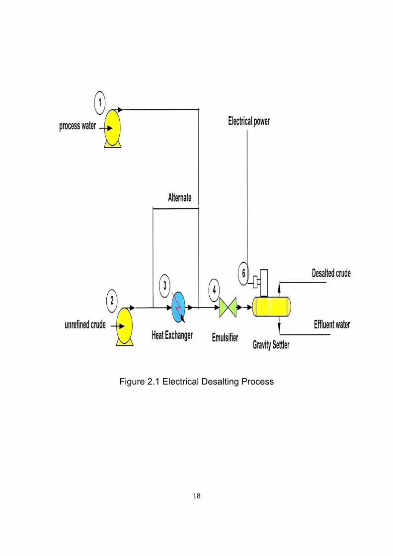
Based on the salt containing situation of crude oil, before entering
tank, crude oil exchanges heat (Figure 2.1) and then is filled with
water. With proper strength mixing, the salts in crude oil are dissolved
in water. Water exists in crude oil in emulsified state. By the
polarization of high-tension electric field, the middle and small water
droplets in the crude oil emulsion are accumulated to form large
water droplets based on density difference between oil and water.
Water droplets settle down in the crude oil, and the salts are
dissolved in water to be removed together with water.
15
I. Water crude separation The difference of density between crude oil and water is the impetus
of settlement separation, and the viscosity of dispersing media is the
resistance. The settlement separation of oil and water insoluble with
each other, is according with tours law for the free settlement of
spherical particulate in static liquid, [7] i.e.:
WC= d² (ρ1- ρ2)* g/18v p2 (2.4)
Where:
WC = settling velocity of water droplets, m/s
D =diameter of water droplets, m
ρ1, ρ2 =density of water and oil, kg/m3
ν = kinematics viscosity of oil, m2/s
g = gravitational acceleration, m/s²
Equation (2.4) is only fitted for the situation where the relative
movement of two phases belongs to laminar flow zone.
Increase in density difference and reduction of viscosity of dispersing
media are in favor of accelerating settling separation, and the two
parameters mainly have relation with the characteristic of crude oil
and the residing temperature. When temperature is increased, the
viscosity of crude oil is reduced, moreover, the decrease of water
density with decrease in temperature is less than that of crude oil,
and thus the increasing temperature is in favor of settling and
16
therefore the separation of oil and water phases. When the
temperature is too high the vaporization of light components in crude
oil and that of water can be avoided a high operating pressure is
adopted for desalting drum. The settling velocity of water droplets is
directly proportion to the square of water droplet diameter. So, the
increase in the diameter of water droplet can greatly accelerate its
settling velocity. Therefore, during the electric desalting of crude oil,
the most important issue is to promote the coalescence of water
droplet to increase its diameter.
II. Function of the electric field The addition of demulsifier to crude oil and the application of heat
settlement methods will not usually meet the requirements of
desalting and dehydration. Moreover, it will take long time and require
large equipment size. The desalting and dehydration process
therefore utilizes high-tension electric field, named electric desalting
process.
The micro water droplets in emulsion can always be induced to have
charges with different polar on the two ends which will generate
inducing dipoles. The micro water droplets contacting with poles will
be charged with static charge, thereby, electrostatic force will be
generated between water droplets and polar .The electrostatic force
can lead the coalescence of micro droplet in what is known as
coalescence forces. Dipole coalescence force of two water droplets
with the same size in high-tension field is [7]:
17
F=6KE 2R2(R/L) 4 (2.5)
Where:
F = Dipole coalescence force.
K = dielectric constant of crude oil.
E = Electric-field intensity.
R = Radius of water droplet.
L = central distance of two water droplets.
The ratio of R to L is the most important factor affecting coalescence
force .R/L is in directly proportional to the cubic root of the dispersion
phase percent content in the emulsion. In order to decrease the salt
content in crude oil, firstly water should be added to dilute the salt
concentration and increase the content of dispersion phase.
The coalescence force is directly proportional to the square of
electric –field intensity E. However it does not mean E can be
infinitely increased to accelerate the coalescence of water droplets,
since coalescence of water droplets high-tension electric field can
also cause the dispersion of water droplets. Figure 2.1 explains how the electrical desalting process works.
18
Figure 2.1 Electrical Desalting Process
19
2.3.3 Filtration method A third and less-common process involves filtering heated crude
using diatomaceous earth. In this method, the feedstock crude oil is
heated to between 150˚and 350˚F to reduce its viscosity and surface
tension for easier mixing and separation of its water content. The
temperature is limited by the vapor pressure of the crude oil
feedstock.
The three methods of desalting may involve the addition of other
chemicals to improve the separation efficiency. Ammonia is often
used to reduce corrosion. Caustic soda or acid may be added to
adjust the pH of the water wash.
Waste water and contaminants are discharged from the bottom of the
setting tank to the waste water treatment facility. The desalted crude
is continuously drawn from the top of the settling tanks and sent to
the crude distillation (fractionating) tower. In desalting process;
control is necessary to avoid any problems that can make the
desalting process failed.
2.4 Control Historical Background For many years process control was an art rather than a science.
Design engineers calculated equipment size to give a certain steady
state performance, but the control systems were chosen by rules of
thumb rather than dynamic analysis. Usually the instrument could be
20
adjusted to give results as good as or better than manual control, and
this was considered adequate. When control found unreliable, the
instruments seeing devices, or the process itself was changed by trial
and error methods until satisfactory solution was found.
Theoretical papers on process control started to appear about 1930.
Grebe, Boundy and Cermak discussed some difficultly of pH control
problems and showed the advantages of using controllers with
derivative action. Evanoff introduced the concept of potential
deviation and potential correction as an aid of quantitative evaluation
of control systems. Callender, Hartree and Porter showed the effect
of time delay on the stability and speed of response of control
system. Minorsky conceded the use of professional, derivative, and
second derivative controllers for steering ship and showed how the
stability could be determined from the differential equations. Hazan
introduces the term "servomechanisms" for position control devices
and discussed the design of control systems capable of closely
following a changing set point. Nyquist developed a general and
relatively simple procedure for determining the stability of feedback
systems from the response of the open loop system.
A great deal of work was done during the World War II to develop
servomechanisms for direction ships, airplanes, guns, and radar
antennas. After the war, several texts appear incorporating these
advances, and courses in servomechanisms became a standard part
of electrical engineering training.
Although the basic principles of feedback control can be applied to
chemical process as well as amplifiers or servomechanisms,
21
chemical engineers have been slow to use the wealth of control
literature from other fields in the design of process control systems.
The unfamiliar terminology is one reason for the delay, but there are
also basic differences between chemical processes and
servomechanisms, which have delayed the development of process
control as a science.
Process control system usually operates with constant set point, and
large-capacity elements help to minimize the effect of disturbances,
whereas they would tend to slow the response of servomechanisms.
Time delay or transportation lag is frequently a major factor in
process control; yet it's hardly mentioned in many servomechanisms
texts. Process control system, interacting first-order elements and
distributed resistances are more frequent than second-order
elements, just the opposite of the machinery control. These
differences make many of published servomechanisms design of little
use to those interested in process control. Inspite of the time delays,
the large time constants, the non linear elements, it's fairly easy to
achieve reasonably good control of most chemical processes.
Furthermore the set point is usually constant, and other controllers
regulate some of the inputs, and so the main control system has to
compensate only for small load changes. The lengthy analysis
needed for accurate design can't be adjusted for such cases, and the
control system is selected by using rule of thumb or shortcut design
procedures.
For complex processes that need closed control, the weakest part of
the control design is usually the dynamic data for the process. The
22
lack of accurate information on process dynamics is still a major
factor limiting the use of process control theory.
As more studies of equipment dynamics becomes available, dynamic
analysis will be more widely use in studying existing equipment and in
designing controllers for few process. The economic justifications will
come mainly from improvement in productivity or product quality,
improvements which might seem small on a percentage basis but
which could save thousands of dollars per year because of the large
quantities produced. Reduction of manpower requirements was one
of the early justifications for automatic control, but there is not much
room left for further economics. Dynamic analysis can show that
controllers are really needed and can lead to quantitative comparison
of proposed control schemes. [8]
2.5 Design Aspects of a process control system 2.5.1 Classifications of the variables: The variables (temperature t, pressure p, concentration C) associated
with a chemical plant, they are divided to:
Input variables, which denote the effect of the surroundings on the
chemical process, are divided to:
1- Manipulated (adjustable), if their values can be adjusted freely by
the human operator or a control mechanism.
23
2- Disturbances, if their values aren’t t adjustable by an operator or
control system.
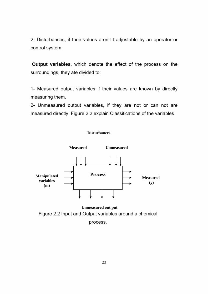
Output variables, which denote the effect of the process on the
surroundings, they ate divided to:
1- Measured output variables if their values are known by directly
measuring them.
2- Unmeasured output variables, if they are not or can not are
measured directly. Figure 2.2 explain Classifications of the variables
2.5.2 Design elements of a control system
Process
Manipulated
variables (m)
Figure 2.2 Input and Output variables around a chemical
process.
Measured (y)
UnmeasuredMeasured
Disturbances
Unmeasured out put
24
2.5.2 Design elements of a control system
1. Define control objective, to design a control system that
satisfies the chemical process, the operational objectives of the
system should be determined.
2. Select measurement of the chemical process, certain variables
should be measured (T, P, F….) which represent the control
objectives on the operation performance. This is done
whenever it’s possible. Such measures are called primary
measurements.
If the control objective variables aren’t measurable quantities or
the measuring devices either are very costly or very low reliability
for the industry, other variables with mathematical relations
(material, energy, balance) can be measured easily and reliably
and the values of the objectives variables by the relations can be
foound. Such supporting measurements are called secondary
measurements.
The behavior of the chemical plant can be monitored by
measuring the disturbances before they enter the process, which
allows knowing in a priori what the behavior will be and thus take
remedial control action to alleviate any undesired consequences.
This measurement is used in feed-forward control.
25
2.5.3 Selection of manipulated variables In the process there are a number of input variables, which can be
adjusted freely. Some will selected as manipulated variables by
determination of degrees of freedom, as the choice will affect the
quality of the control action.
2.5.4 Selection of the control configuration Selection of the control configuration depends on how many
controlled outputs in the plant. It can be distinguish as either single
input single output (SISO) or multiple inputs multiple outputs (MIMO).
Feedback control configuration uses direct measurements of the
controlled variables (measured outputs) to adjust the values of the
manipulated variables. The objective is to keep the controlled
variables at desired levels.
Inferential control configuration uses secondary measurements to
adjust the values of the manipulated variables. The objective are
to keep (the unmeasured) controlled variables at desired level.
Feed forward control configuration uses direct measurement of the
disturbances to adjust the values of the manipulated variables –
the objective is to keep the values of the controlled outputs at
desired level. [1]
26
2.6 Controllers The controller is a device which monitors and affects the operational
conditions of a given dynamical system. The operational conditions
are typically referred to as output variables of the system which can
be affected by adjusting certain input variables. It receives the
information from the measuring device and decides what action
should be taken.
2.7 Types of continuous controllers 2.7.1 Proportional controller (P- controller)
In this type of controller, the controller output (control action) is
proportional to the error in the measured variable. The error is
defined as the difference between the current value (measured) and
the desired value (set point). If the error is large, then the control
action is large.
Mathematically:
C (t) α Kc * e (t) → C (t) = Kc * e (t) + CS (2.6)
Where:
e (t) ≡ the error
Kc ≡ the controller's proportional gain
27
CS ≡ the steady state control action (necessary to
maintain the variable at the steady state when there is no error)
C (t) = Kc * e (t) (2.7)
The transfer function is
( ) ( ) / ( ) cG s c s E s k= = (2.8)
Proportion action repeats the input signal and produces a continuous
action.
The gain Kc will be positive if an increase in the input variable requires
an increase in the output variable (direct-acting control), and it will be
negative if an increase in the input variable requires a decrease in the
output variable (reverse-acting control).
Proportional action decreases the rising time making the
response faster, but it causes instability by the overshooting (offset).
2.7.2 Integral controller (I- controller) Also, known as reset controller, this type of controller, the controller
output (control action) is proportional to the integral of the error in the
measured variable.
28
The transfer function is:
( ) ( ) / ( ) (1/ )c iG s c s E s k sτ= = (2.9)
Where:
Kc = the controller’s proportional gain.
iτ =integral time.
Integral action has a higher overshoot than the proportional due to its
slow starting behavior, but no steady state error (no offset).
2.7.3 Derivative Controller (D-Controller) In this type of controller, the controller output (control action) is
proportional to the rate of change in error (error derivative) in the
measured variable.
Kc ≡ the controller proportional gain.
dτ ≡ derivative time constant in minutes.
The transfer function is:
( ) ( )/ ( ) (2 .10)c dG s c s E s k sτ= =
29
2.7.4 PI Controller In this type of controller, the controller output (control action) is
proportional to the rate of change in error and the integral of the error
in the measured variable.
Initially the controller output is the proportional action (integral
contribution is zero) after a period of it mints the contribution of the
integral action starts.
The integral action repeats the response of the proportional action
causes the output to changing continuously as long as the error is
existing. Reset time is the time needed by the controller to repeat the
initial proportional action change output.
The transfer function:
( ) ( )/ ( ) (1 1/ ) (2 .11)c iG s c s E s k sτ= = +
2.7.5 PD Controller
In this type of controller, the controller output (control action) is
proportional to summation of the error and rate of change in error in
the measured variable.
The transfer function:
( ) ( )/ ( ) (1 )c dG s c s E s k sτ= = + (2.12)
30
Derivative time is the time taken by the proportional action to
reproduce the initial step of the derivative action.
2.7.6 PID Controller
In this type of controller, the controller output (control action) is
proportional to summation of the error and rate of change in error and
the integral of the error in the measured variable.
The integral action will provide the automatic reset to eliminate offset
following a load change. The derivative action will improve the system
stability, which results in reducing the peak deviation as well as
providing a faster recovery. Increasing the integral action will
eliminate the offset in shorter time, but as it decrease the stability it
leads to longer recovery time. Hence some compromise is necessary
between the rate of recovery and the offset and the overall recovery
time.
The transfer function is:
( ) ( )/ ( ) (1 1/ )c i dG s c s E s k s sτ τ= = + + (2.13)
2.8 Controller tuning The controller is the active element that receives the information from
the measurements and takes appropriate control actions to adjust the
31
value of the manipulated variables taking the best response of the
process using different controller laws.
In order to be able to use a controller, it must first be tuned to the
system. This tuning synchronizes the controller with the controlled
variable, thus allowing the process to be kept at its desired operating
condition.
2.8.1 Open Loop tuning
Open-Loop tuning method is a way of relating the process
parameters (delay time, process gain, and time constant) to the
controller parameters (controller gain and reset time). It has been
developed for use on delay followed by first order lag processes but
can also be adapted to other processes, similar to those encountered
in industry.
2.8.2 Closed loop tuning
In some real processes the response to a step change or set point
disturbance differs depending on the direction or size of the change.
In this case it is irrelevant to look at the open-loop response to tune
the controller; instead the closed-loop response is used. The method
looks at the response of the system under proportional control. The
method looks more rebuts because it does not require a specific
process model.
32
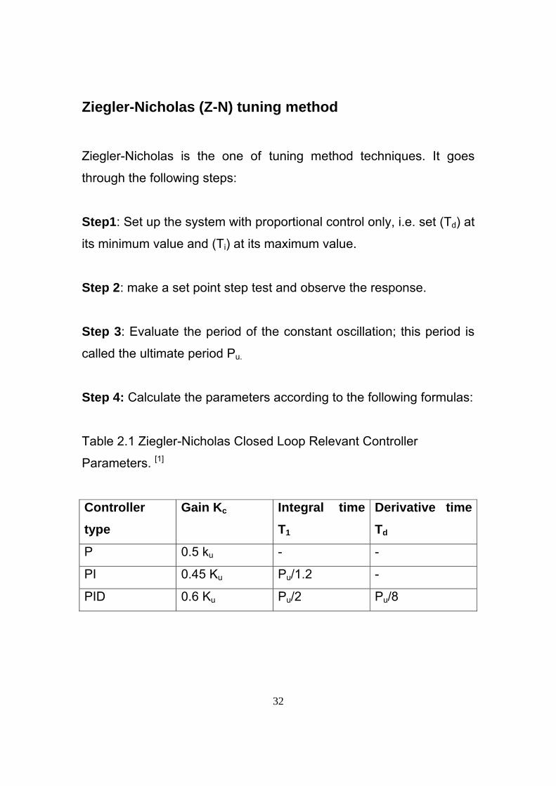
Ziegler-Nicholas (Z-N) tuning method Ziegler-Nicholas is the one of tuning method techniques. It goes
through the following steps:
Step1: Set up the system with proportional control only, i.e. set (Τd) at
its minimum value and (Τi) at its maximum value.
Step 2: make a set point step test and observe the response.
Step 3: Evaluate the period of the constant oscillation; this period is
called the ultimate period Pu.
Step 4: Calculate the parameters according to the following formulas:
Table 2.1 Ziegler-Nicholas Closed Loop Relevant Controller
Parameters. [1]
Controller type
Gain Kc Integral time T1
Derivative time Td
P 0.5 ku - -
PI 0.45 Ku Pu/1.2 -
PID 0.6 Ku Pu/2 Pu/8
33
2.9 Stability
Stability is the state or quality of being stable. It can also be defined
as a resistance to change, determination, or displacement,
consistency of character or purpose; steadfastness; reliability,
dependability; the ability of an object, such as a ship or aircraft, to
maintain equilibrium or resume its original, upright position after
displacement, as by the sea or strong winds; the condition of being
stable or resistance to change; the quality or attribute of being stable;
the quality free from change or variation.
In mathematics, a condition in which slight disturbances in a system
does not produce a significant disrupting in effect on that system. A
solution to a differential equation is said to be stable if a slightly
different solution that is close to it when x = 0 remains close for
nearby values of x. Stability of solutions is important in physical
applications because deviations in mathematical models inevitably
result from errors in measurement. A stable solution will be usable
despite such deviations. The transient response of a feedback control
system is of primary interest and must be investigated. A very
important characteristic of transient performance of a system is its
stability. If a control system is satisfactory it should meet the following
requirements:
1- Stability by showing stable behavior.
2-Good control quality or good dynamics which deals with transient
response. [1]
34
2.10 Concept of stability A stable system is one that will remain at rest unless excited by an
external source and will return to rest if all excitations are removed.
Dynamically the system stability is determined by its response to
inputs or disturbance. A system is considered stable if its response is
bounded, or if every bounded input produces a bounded output.
If some excitation causes the outputs to increase continuously or to
oscillate with growing amplitude, it is as unstable system.
2.11 Stability techniques The system stability can be tested by considering its response to a
finite input signal. Several methods have been developed to deduce
the system stability from its characteristic equation. The direct method criterion is shortcut methods for assessment of the
stability of a system by providing information from the S-domain
without finding out the actual response of a system in the time
domain.
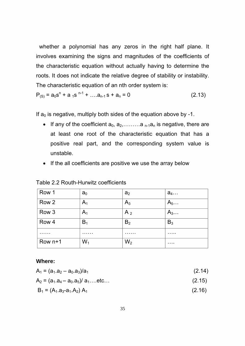
2.12 Methods-techniques for stability 2.12.1 Routh-Hurwitz criteria Routh-Hurwitz criteria is an algebraic procedure for determining
35
whether a polynomial has any zeros in the right half plane. It
involves examining the signs and magnitudes of the coefficients of
the characteristic equation without actually having to determine the
roots. It does not indicate the relative degree of stability or instability.
The characteristic equation of an nth order system is:
P(S) = a0sn + a 1s n-1 + ….an-1 s + an = 0 (2.13)
If a0 is negative, multiply both sides of the equation above by -1.
• If any of the coefficient a0, a2,………a n-1an is negative, there are
at least one root of the characteristic equation that has a
positive real part, and the corresponding system value is
unstable.
• If the all coefficients are positive we use the array below
Table 2.2 Routh-Hurwitz coefficients
Row 1 a0 a2 a4…
Row 2 A1 A3 A5…
Row 3 A1 A 2 A3…
Row 4 B1 B2 B3
…… …… …… …..
Row n+1 W1 W2 ….
Where: A1 = (a1.a2 – a0.a3)/a1 (2.14)
A2 = (a1.a4 – a0.a5)/ a1….etc… (2.15) B1 = (A1.a3-a1.A2) A1 (2.16)
36
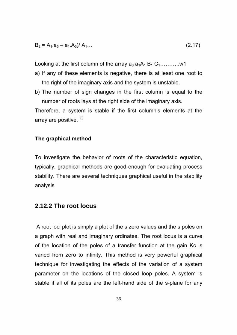
B2 = A1.a5 – a1.A3)/ A1… (2.17)
Looking at the first column of the array a0 a1A1 B1 C1………..w1
a) If any of these elements is negative, there is at least one root to
the right of the imaginary axis and the system is unstable.
b) The number of sign changes in the first column is equal to the
number of roots lays at the right side of the imaginary axis.
Therefore, a system is stable if the first column's elements at the
array are positive. [8]
The graphical method
To investigate the behavior of roots of the characteristic equation,
typically, graphical methods are good enough for evaluating process
stability. There are several techniques graphical useful in the stability
analysis
2.12.2 The root locus A root loci plot is simply a plot of the s zero values and the s poles on
a graph with real and imaginary ordinates. The root locus is a curve
of the location of the poles of a transfer function at the gain Kc is
varied from zero to infinity. This method is very powerful graphical
technique for investigating the effects of the variation of a system
parameter on the locations of the closed loop poles. A system is
stable if all of its poles are the left-hand side of the s-plane for any
37
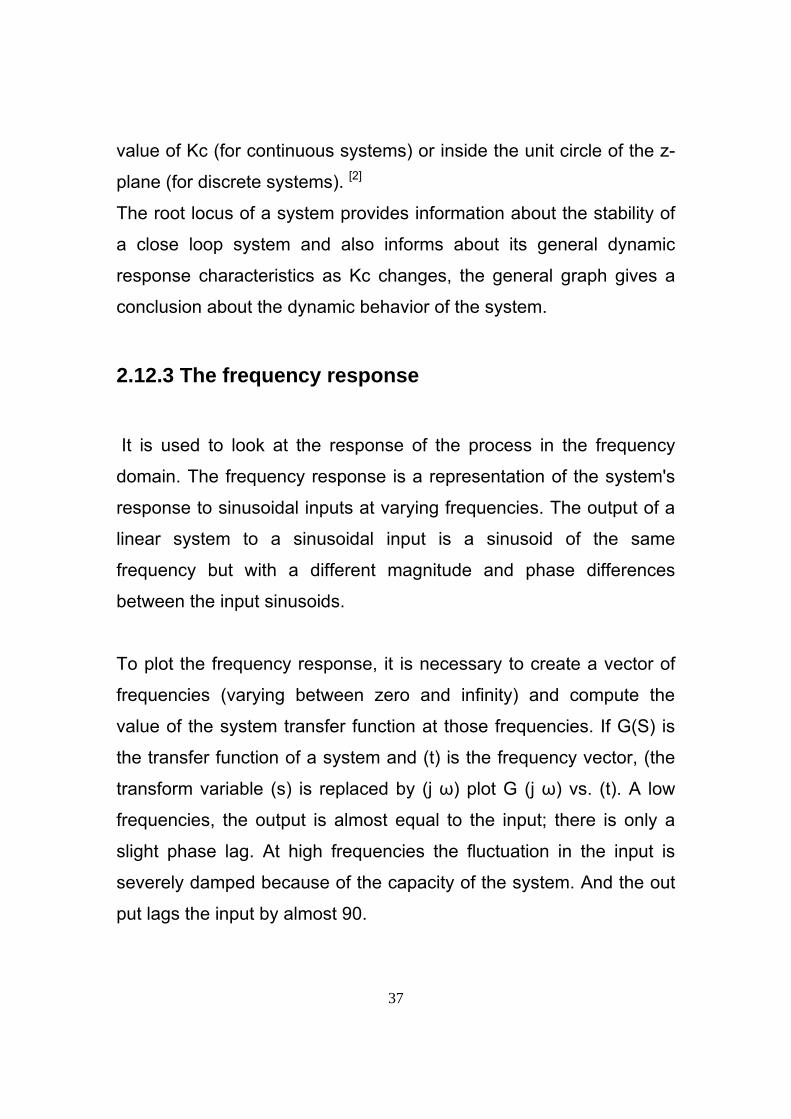
value of Kc (for continuous systems) or inside the unit circle of the z-
plane (for discrete systems). [2]
The root locus of a system provides information about the stability of
a close loop system and also informs about its general dynamic
response characteristics as Kc changes, the general graph gives a
conclusion about the dynamic behavior of the system.
2.12.3 The frequency response It is used to look at the response of the process in the frequency
domain. The frequency response is a representation of the system's
response to sinusoidal inputs at varying frequencies. The output of a
linear system to a sinusoidal input is a sinusoid of the same
frequency but with a different magnitude and phase differences
between the input sinusoids.
To plot the frequency response, it is necessary to create a vector of
frequencies (varying between zero and infinity) and compute the
value of the system transfer function at those frequencies. If G(S) is
the transfer function of a system and (t) is the frequency vector, (the
transform variable (s) is replaced by (j ω) plot G (j ω) vs. (t). A low
frequencies, the output is almost equal to the input; there is only a
slight phase lag. At high frequencies the fluctuation in the input is
severely damped because of the capacity of the system. And the out
put lags the input by almost 90.
38
The capacity response of a system can be viewed in two different
ways: via the Bode plot or via the Nyquist diagram. Both methods
display the same information; the difference lies in the way the
information is presented. [8]
2.12.4 Nyquist plot Nyquist plot are used to analyze system properties including gain
margin, phase margin, stability, and for assessing the stability of a
system with feedback. It is represented by a graph in polar
coordinates in which the gain and phase of frequency response are
plotted, the gain is plotted as the radius vector and the phase shift is
plotted in degrees clockwise from the right hand abscissa. There is a
separate point for each frequency; the frequencies are indicated next
to a few of the point, or a narrow is used to show the direction of
increasing frequency. [1]
2.12.5 Bode plot
A graphical method consists of plotting two curves to present the
response of open loop at variance frequencies. It is used to
determine the stability limits of the closed loop system, the critical
frequency of the system, and to predict the optimum controller
setting. The response presented at a log-log plot for the amplitude
ratios, accompanied by the simi-log plot for the phase angle. [1]
39
2.13 Types of control systems There are several types of control systems
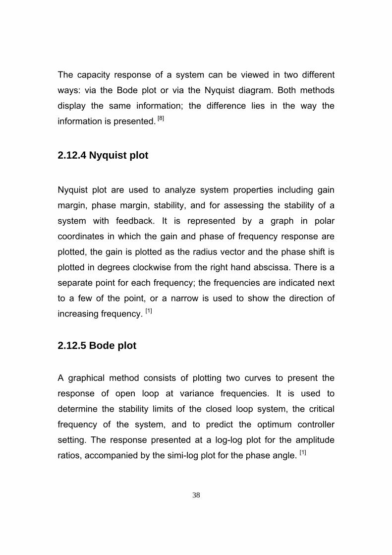
2.13.1 Feed-forward control system
Feed-forward control is a strategy used to compensate for
disturbances in a system before they affect the control variable. A
feed forward control systems measures a disturbance variable,
predicts it is effect on the process, and applies corrective action.
(Figure 2.3).
Figure 2.3 Open loop control system.
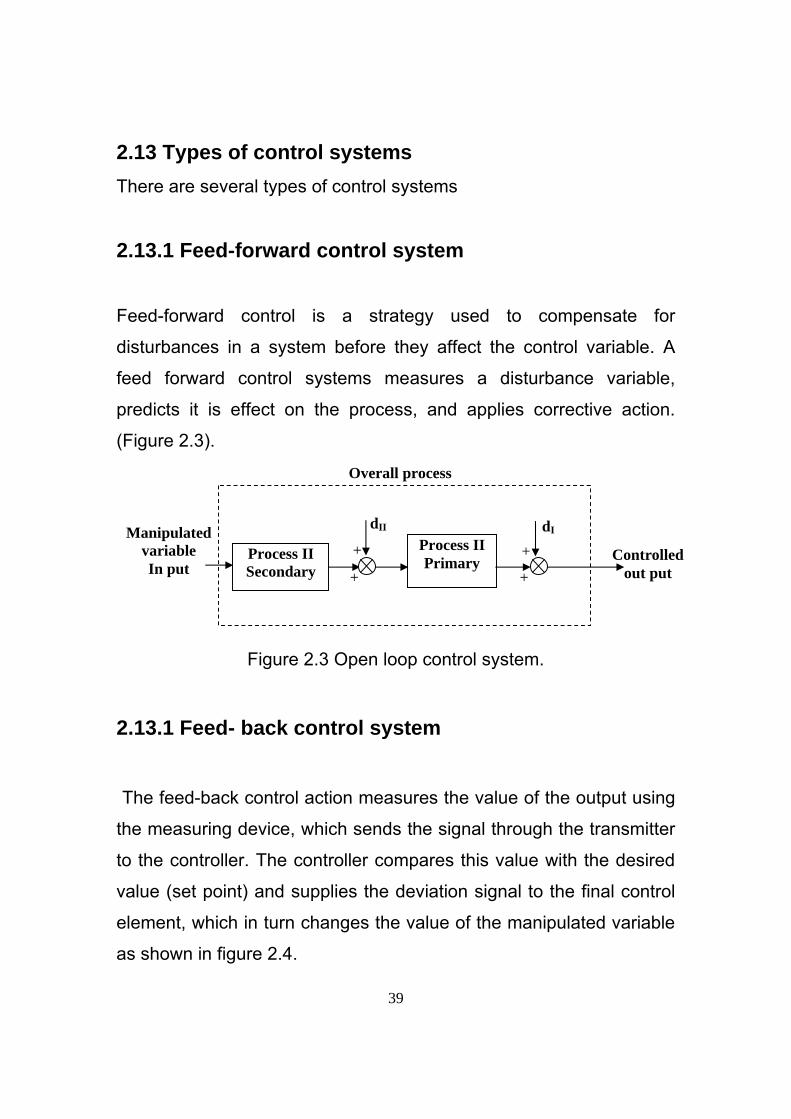
2.13.1 Feed- back control system
The feed-back control action measures the value of the output using
the measuring device, which sends the signal through the transmitter
to the controller. The controller compares this value with the desired
value (set point) and supplies the deviation signal to the final control
element, which in turn changes the value of the manipulated variable
as shown in figure 2.4.
Process II Secondary
Process II Primary
Overall process
Controlled out put
Manipulated variable In put
dI +
+
dII
+
+
40
Figure 2.4 Feed Back Control System
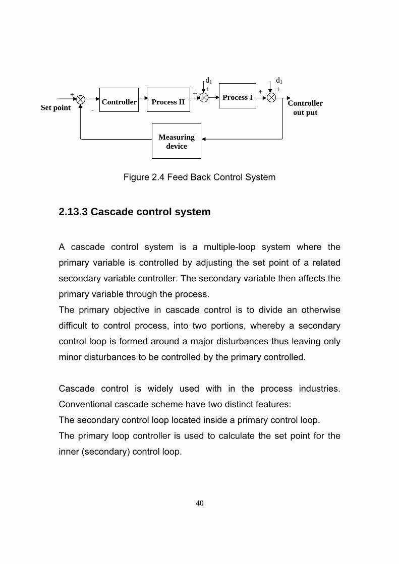
2.13.3 Cascade control system
A cascade control system is a multiple-loop system where the
primary variable is controlled by adjusting the set point of a related
secondary variable controller. The secondary variable then affects the
primary variable through the process.
The primary objective in cascade control is to divide an otherwise
difficult to control process, into two portions, whereby a secondary
control loop is formed around a major disturbances thus leaving only
minor disturbances to be controlled by the primary controlled.
Cascade control is widely used with in the process industries.
Conventional cascade scheme have two distinct features:
The secondary control loop located inside a primary control loop.
The primary loop controller is used to calculate the set point for the
inner (secondary) control loop.
Measuring
device
Controller
Process II
Process I
Set point + + +
d1 +
Controller out put
d1 +
-
41
Cascade control is used to improve the response of a signal feedback
strategy. The secondary control loop is located so that it recognizes
the upset condition sooner than the primary loops. (Figure 2.5).
Figure 2.5 Cascade Control System
Secondary controller
Process II
Measuring device
Primary controller
Process I
Secondary loop
Primary loop
Controlled out put
Set point - - +
+ +
+
+
dI + dII
Measuring device
42
Chapter Three
Materials and Methods
43
Materials and Methods
This chapter will represent some definitions for: Cascade control instruments,
Feed back control instruments, controller action, stability criterions, types of
sensors, mathematical model and component balance.
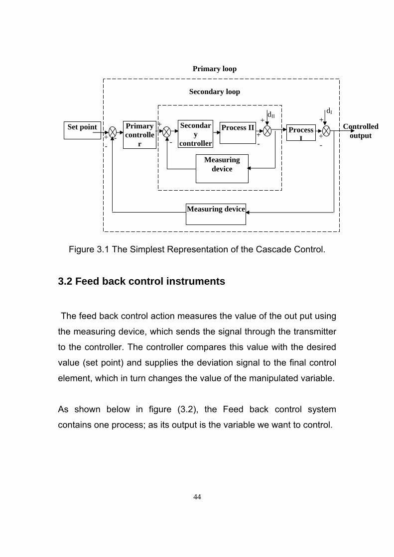
3.1 Cascade control instruments A cascade control system is a multiple-loop system where the
primary variable is controlled by adjusting the set point of a related
secondary variable controller. The secondary variable then affects the
primary variable through the process.
As shown in figure (3.1) below the cascade control system contains
two processes.
Process1: (Primary loop) has as its output the variable we want to
control.
Process 2: (Secondary loop) has an output that we are not interested
in controlling but which affects the output we want to control.
44
Figure 3.1 The Simplest Representation of the Cascade Control.
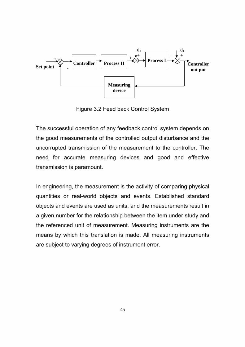
3.2 Feed back control instruments
The feed back control action measures the value of the out put using
the measuring device, which sends the signal through the transmitter
to the controller. The controller compares this value with the desired
value (set point) and supplies the deviation signal to the final control
element, which in turn changes the value of the manipulated variable.
As shown below in figure (3.2), the Feed back control system
contains one process; as its output is the variable we want to control.
Secondary
controller
Process II
Measuring device
Primary controlle
r
Process I
Secondary loop
Primary loop
Controlled output
Set point - -
+-
+
+-
+
+-
dI
+dII
Measuring device
45
Figure 3.2 Feed back Control System
The successful operation of any feedback control system depends on
the good measurements of the controlled output disturbance and the
uncorrupted transmission of the measurement to the controller. The
need for accurate measuring devices and good and effective
transmission is paramount.
In engineering, the measurement is the activity of comparing physical
quantities or real-world objects and events. Established standard
objects and events are used as units, and the measurements result in
a given number for the relationship between the item under study and
the referenced unit of measurement. Measuring instruments are the
means by which this translation is made. All measuring instruments
are subject to varying degrees of instrument error.
Measuring
device
Controller
Process II
Process I
Set point + + +
d1 +
Controller out put
d1 +
-
46
3.3 The controller action
In This study proportional action only will used and the transfer
function is:
( ) ( ) / ( ) cG s c s E s k= = (2.8)
Proportion action repeats the input signal and produces a continuous
action.
The gain Kc will be positive if an increase in the input variable requires
an increase in the output variable (direct-acting control), and it will be
negative if an increase in the input variable requires a decrease in the
output variable (reverse-acting control).
Proportional action decreases the rising time making the
response faster, but it causes instability by the overshooting (offset).
3.4 The stability criterions 3.4.1 Bode Criterion A feed back control system is stable according to bode criterion if the
amplitude ratio of the corresponding open-loop transfer function is
less than one at the crossover frequency.
The crossover frequency is the frequency where the phase lag is
equal to (- 180 )˚ .
47
3.4.2 Nyguist stability criterion
It states that if the open-loop Nyguist plot of feed back system
encircles the point (- 1.0) as the frequency w takes any value from (-
∞ to + ∞).
3.4.3 Root locus criterion
This criterion of stability does not require calculations of the actual
values of the roots of the characteristic equation, it is only requires
that we know if any root is to the right of the imaging axis (i.e., have
positive real part) that leads to unstable system.
3.5 Sensors A sensor is a type of transducer. Sensors are used in innumerable
applications; include automobile, machines, aerospace, medicine,
industry, and robotics.
Sensors are electrical or electronic, although other types exist
sensors. Sensitivity indicates how much the sensor's output changes
when the measured quantity changes, if the mercury in a
thermometer moves 1cm when the temperature changes by 1oc, the
sensitivity is then 1cm/1oc. Sensors that measure very small changes
must have very high sensitivities. Technological progress allows more
and more sensors to be manufactured on a microscopic scale. In
48
most cases, a micro sensor reaches a significantly higher speed and
sensitivity compared with macroscopic approaches.
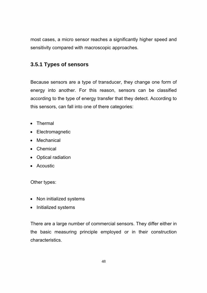
3.5.1 Types of sensors
Because sensors are a type of transducer, they change one form of
energy into another. For this reason, sensors can be classified
according to the type of energy transfer that they detect. According to
this sensors, can fall into one of there categories:
• Thermal
• Electromagnetic
• Mechanical
• Chemical
• Optical radiation
• Acoustic
Other types:
• Non initialized systems
• Initialized systems
There are a large number of commercial sensors. They differ either in
the basic measuring principle employed or in their construction
characteristics.
49
Process
Variable Measuring device Comments
Orifice plates
Ventura flow nozzle
Dahl flow tube
Dennison flow nozzle
Measuring pressure
drop across a flow
constriction
Turbine flow meters Ultrasound
Flow
Hot wire anemometry For high precision
Float-actuated device
Displacer device
Coupled with various
types of indicators and
signal convectors
Conductivity measurements
Dielectric measurements
Liquid head pressure devices
Sonic resonance
Good for systems with
two phases
Liquid level Potentiometry
Conductmetery
Oscillometeric analyzers
pH meter
polo graphic analyzers
Coulometer Spectrometers (x-ray,
electron, ion, Mossbauer, Raman
etc)
Different thermal analyzes
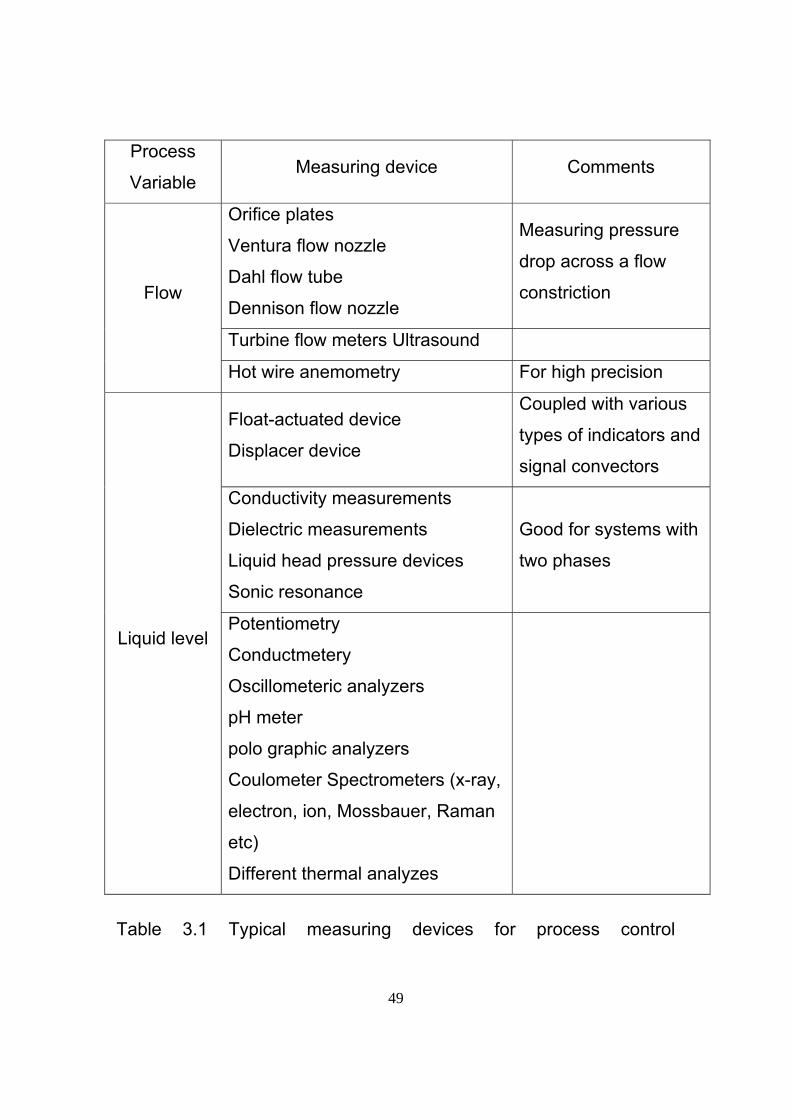
Table 3.1 Typical measuring devices for process control
50
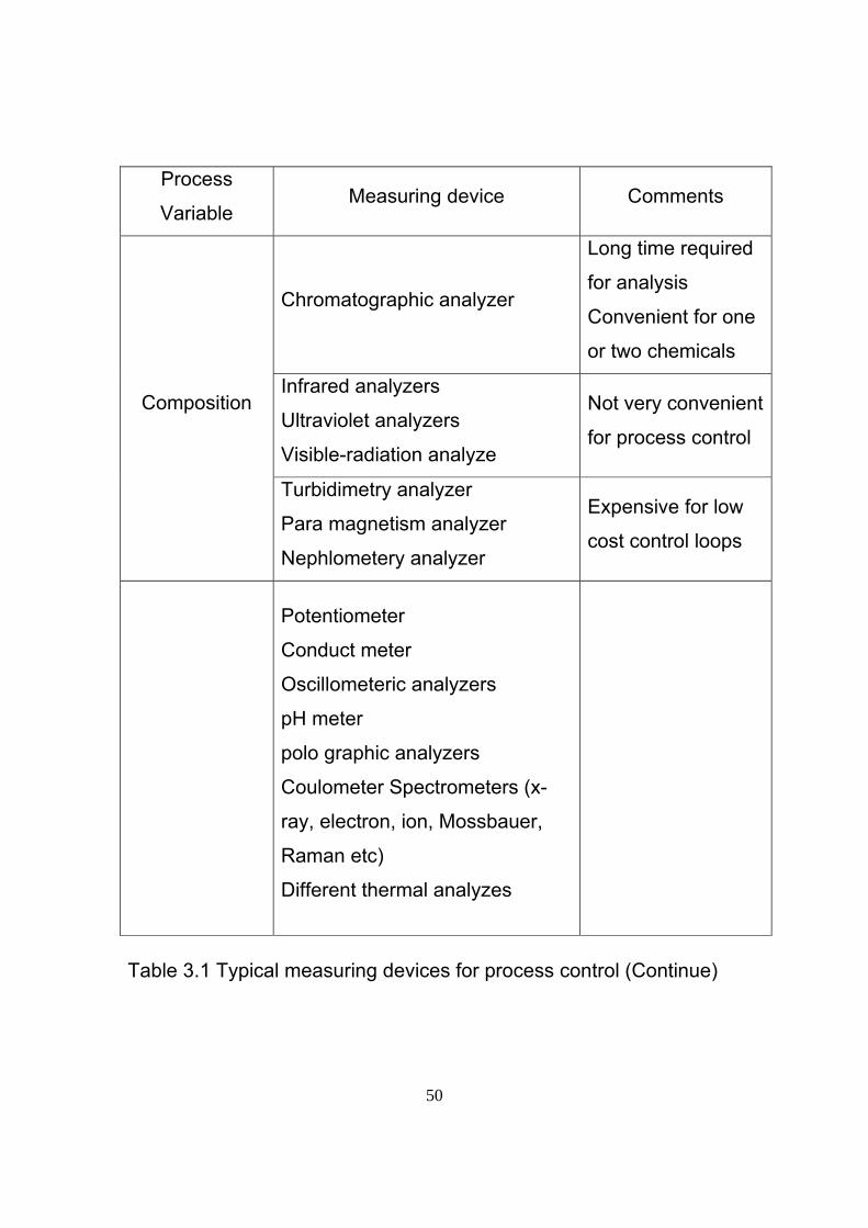
Table 3.1 Typical measuring devices for process control (Continue)
Process
Variable Measuring device Comments
Chromatographic analyzer
Long time required
for analysis
Convenient for one
or two chemicals
Infrared analyzers
Ultraviolet analyzers
Visible-radiation analyze
Not very convenient
for process control
Composition
Turbidimetry analyzer
Para magnetism analyzer
Nephlometery analyzer
Expensive for low
cost control loops
Potentiometer
Conduct meter
Oscillometeric analyzers
pH meter
polo graphic analyzers
Coulometer Spectrometers (x-
ray, electron, ion, Mossbauer,
Raman etc)
Different thermal analyzes
51
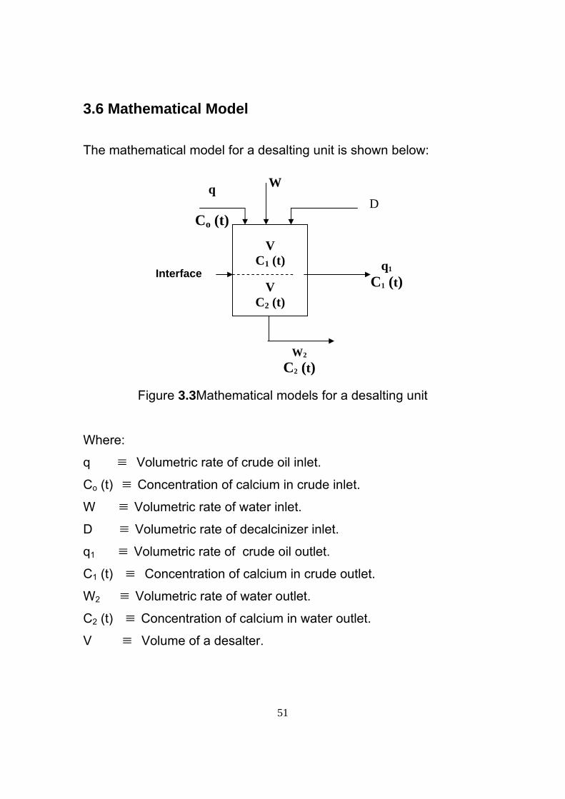
3.6 Mathematical Model The mathematical model for a desalting unit is shown below:
Figure 3.3Mathematical models for a desalting unit
Where:
q ≡ Volumetric rate of crude oil inlet.
Co (t) ≡ Concentration of calcium in crude inlet.
W ≡ Volumetric rate of water inlet.
D ≡ Volumetric rate of decalcinizer inlet.
q1 ≡ Volumetric rate of crude oil outlet.
C1 (t) ≡ Concentration of calcium in crude outlet.
W2 ≡ Volumetric rate of water outlet.
C2 (t) ≡ Concentration of calcium in water outlet.
V ≡ Volume of a desalter.
V
C1 (t)
V C2 (t)
q
Co (t)
D
q1 C1 (t)
W2 C2 (t)
Interface
W
52
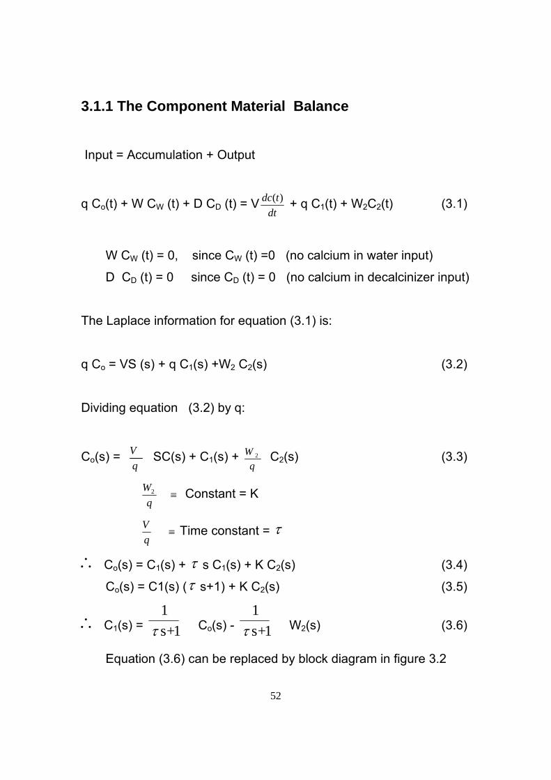
3.1.1 The Component Material Balance Input = Accumulation + Output
q Co(t) + W CW (t) + D CD (t) = Vdt
tdc )( + q C1(t) + W2C2(t) (3.1)
W CW (t) = 0, since CW (t) =0 (no calcium in water input)
D CD (t) = 0 since CD (t) = 0 (no calcium in decalcinizer input)
The Laplace information for equation (3.1) is:
q Co = VS (s) + q C1(s) +W2 C2(s) (3.2)
Dividing equation (3.2) by q:
Co(s) = qV SC(s) + C1(s) +
qW 2 C2(s) (3.3)
q
W2 ≡ Constant = K
qV ≡ Time constant = τ
∴ Co(s) = C1(s) + τ s C1(s) + K C2(s) (3.4)
Co(s) = C1(s) (τ s+1) + K C2(s) (3.5)
∴ C1(s) = 1+s 1
τ Co(s) - 1+s 1
τ W2(s) (3.6)
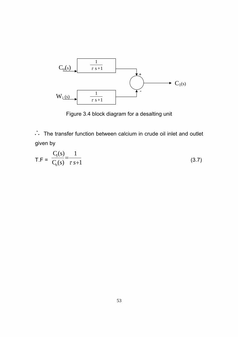
Equation (3.6) can be replaced by block diagram in figure 3.2
53
Figure 3.4 block diagram for a desalting unit
∴ The transfer function between calcium in crude oil inlet and outlet
given by
T.F = 11
(s)C(s)C
o
1
+=
sτ (3.7)
1+s 1
τ
W2 (s)
Co(s)
C1(s)
+
-
1+s 1
τ

54
CHAPTER FOUR
Result and
Discussion
55
Result and Discussion
In this chapter control strategy, stability analysis for two control systems will represent.
This is followed
by stability comparison between two systems. Block diagram for cascade control
using microprocessor and comments are also outlined at the end of this chapter.
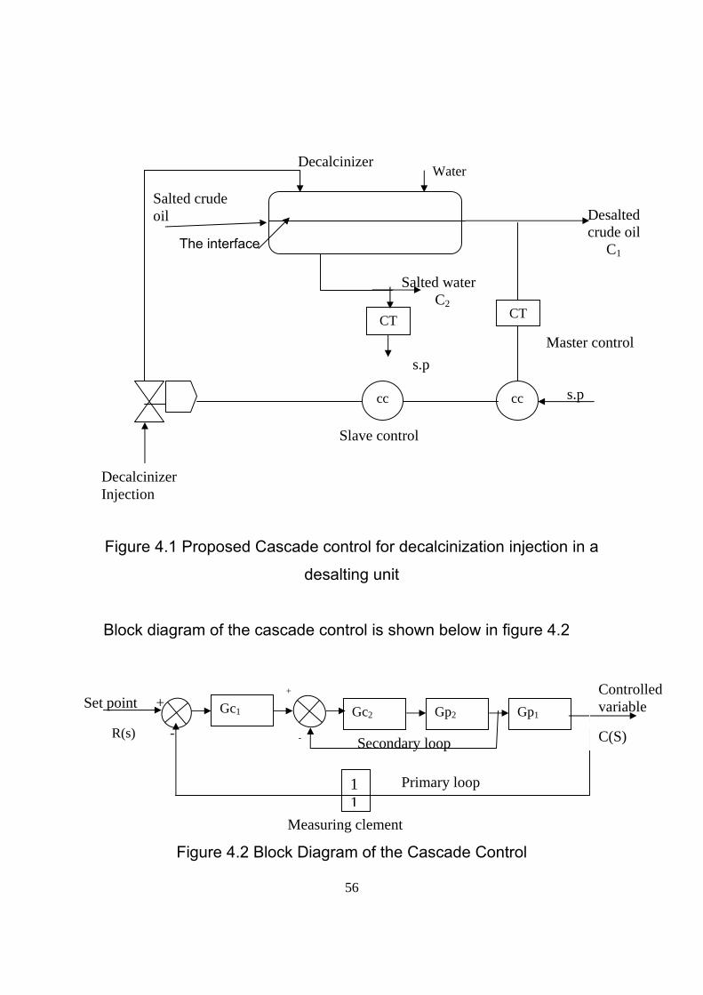
4.1 Control Strategy 4.1.1 Cascade Control Strategy A case study of a control system of a decalcinizer was under taken.
In this study the controlled variables were the composition of calcium
salts in the desalted crude and that in effluent water. The composition
of calcium in the crude oil will be cascaded with the composition of
exit salted water.
The control system proposed to be used is shown in figure (4.1).
56
The interface
Figure 4.1 Proposed Cascade control for decalcinization injection in a
desalting unit
Block diagram of the cascade control is shown below in figure 4.2
Figure 4.2 Block Diagram of the Cascade Control
cc cc
CT CT
Water Decalcinizer
Salted crude oil Desalted
crude oil C1
Salted water C2
s.p
s.p
Slave control
Decalcinizer Injection
Master control
Gp1 Gp2 Gc2 Gc1
R(s) -
Set point +
Secondary loop
Primary loop
Measuring clement
-
+
C(S)
Controlled variable
1 1
57
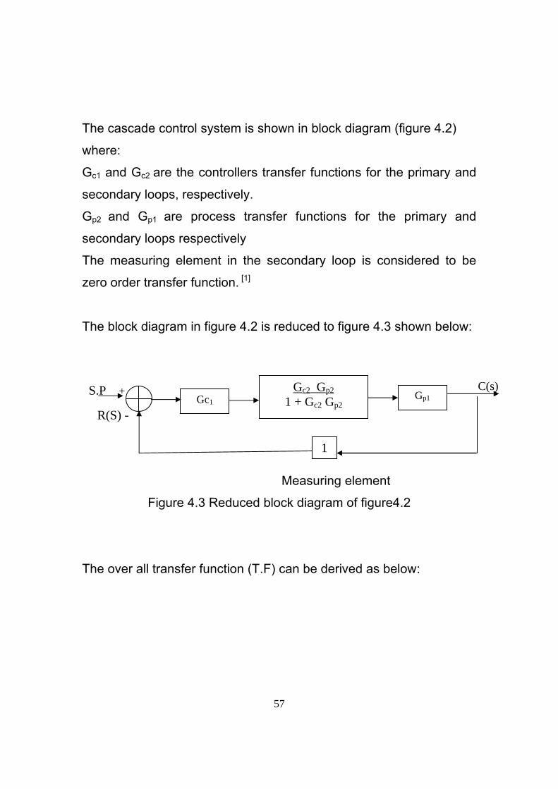
The cascade control system is shown in block diagram (figure 4.2)
where:
Gc1 and Gc2 are the controllers transfer functions for the primary and
secondary loops, respectively.
Gp2 and Gp1 are process transfer functions for the primary and
secondary loops respectively
The measuring element in the secondary loop is considered to be
zero order transfer function. [1]
The block diagram in figure 4.2 is reduced to figure 4.3 shown below:
Measuring element
Figure 4.3 Reduced block diagram of figure4.2
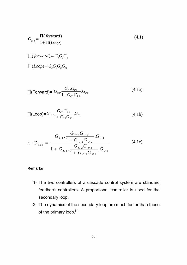
The over all transfer function (T.F) can be derived as below:
Gp1 Gc2 Gp2
1 + Gc2 Gp2 Gc1
1
S.P +
R(S) -
C(s)
58
( )
v
( ) 1 ( )
( )
( )
S
c p
c v p m
forwardGLoop
forward G G G
Loop G G G G
Π=
+Π
∏ =
∏ =
∏(Forward)=
2 21 1
2 2
. . 1
C PC P
C P
G GG GG G+
∏(Loop)= 2 21 1
2 2
. . 1
C PC P
C P
G GG GG G+
2 21 1
2 2( )
2 2 .1 1
2 2
. .1
1 . .1
C PC P
C PS
C PC P
C P
G GG GG GG G GG G
G G
+∴ =
++
Remarks
1- The two controllers of a cascade control system are standard
feedback controllers. A proportional controller is used for the
secondary loop.
2- The dynamics of the secondary loop are much faster than those
of the primary loop.[1]
(4.1)
(4.1a)
(4.1b)
(4.1c)
59
(4.2)
Applying pade approximation [1] :
12
12
d
td
d
t Se t S
−−
=+
11 1
11 1 2. . 1 1 1
2
d
tdsP
dP p
t SG e tS S Sτ τ
−−
∴ = =+ + +
22
1 1P
P
GSτ
∴ =+
21 PP ττ >
The P–action controller will be used in the primary loop. Because the
process is an (on – off) injection and the decalcinizer (Acetic Acid) is
Injected periodically.
1 1
2 2
C C
C C
G KG K
∴ =∴ =
Three assumptions will be used to compare between the cascade
control system and feedback control system. The dead time will be
assumed as one minutes due to the large volume of the desalter
(D=4.2m, L=84m).
DeadTimet
eS
G
d
tds
PP
≡+
=∴ −.1
1
11 τ
(4.2a)
(4.2b)
(4.3)
(4.4)
(4.5)
60
A. Assumption (1):
min1
min1.0min1
2
1
=
==
d
p
P
t
ττ
Substitute these values in equation (4.1) and (4.2) to obtain the
transfer function for primary and secondary process elements
Using pade approximation [1]:
11 1 0.5.
1 1 0.5pSG
S S−
=+ +
21
0.1 1PGS
∴ =+
The secondary loop is faster than the primary, as can be seen from
the corresponding time constants.
For using simple feedback control the open – loop transfer function
with P_Control only is: 1
1 2 1 1
1 2 1 1
1. . 0.1 1 1
1 1 1 0.5. . . (0.1 1) ( 1) (1 0.5 )
S
C P P C
C P P C
eG G G KS S
SG G G KS S S
−
=+ +
−=
+ + +
The cross over frequency can be found from the equation that sets
the total phase lag equal to – 180o
11
1 1 1 0 .5. . 1 1 1 0 .5
sP
SG eS S S
− −∴ = =
+ + +(4.6)
(4.6a)
(4.7)
(4.8)
(4.9)
61
φ = total phase lag = - 180o
w = cross over frequency
≡Pτ Time constant 0 1 11 8 0 ta n ( 0 .1 ) ( ) ta n ( 1 )
2 4 .5 / m inw w w
w r a d
− −∴ − = − + − + −∴ =
The overall amplitude ratio is give by
2
1 ( )P
P
KARwτ
=+
1 2 2
1 1. . (0 .1 ) 1 1
24.5 / m in
CAR Kw w
w rad
∴ =+ +
=
1015.0 CKAR =∴
The ultimate value of the gain k can be found when AR = 1
1 0 . 0 1 5 6 6
K uK u
∴ =∴ =
4.1.2 Controllers Tuning for Cascade System
The Ziegler – Nicholas (Z-N) is used in this research to find the
parameters of the proportional controller of the primary loop.
From (z-n) tuning technique
The controller gain kc1 value is
1tan pwϕ τ−= − (4.9) (4.10) [1]
(4.10a)
(4.11)[1]
(4.11a)
(4.11b)
62
1
1
2
66 332
C
C
KuK
K
=
= =
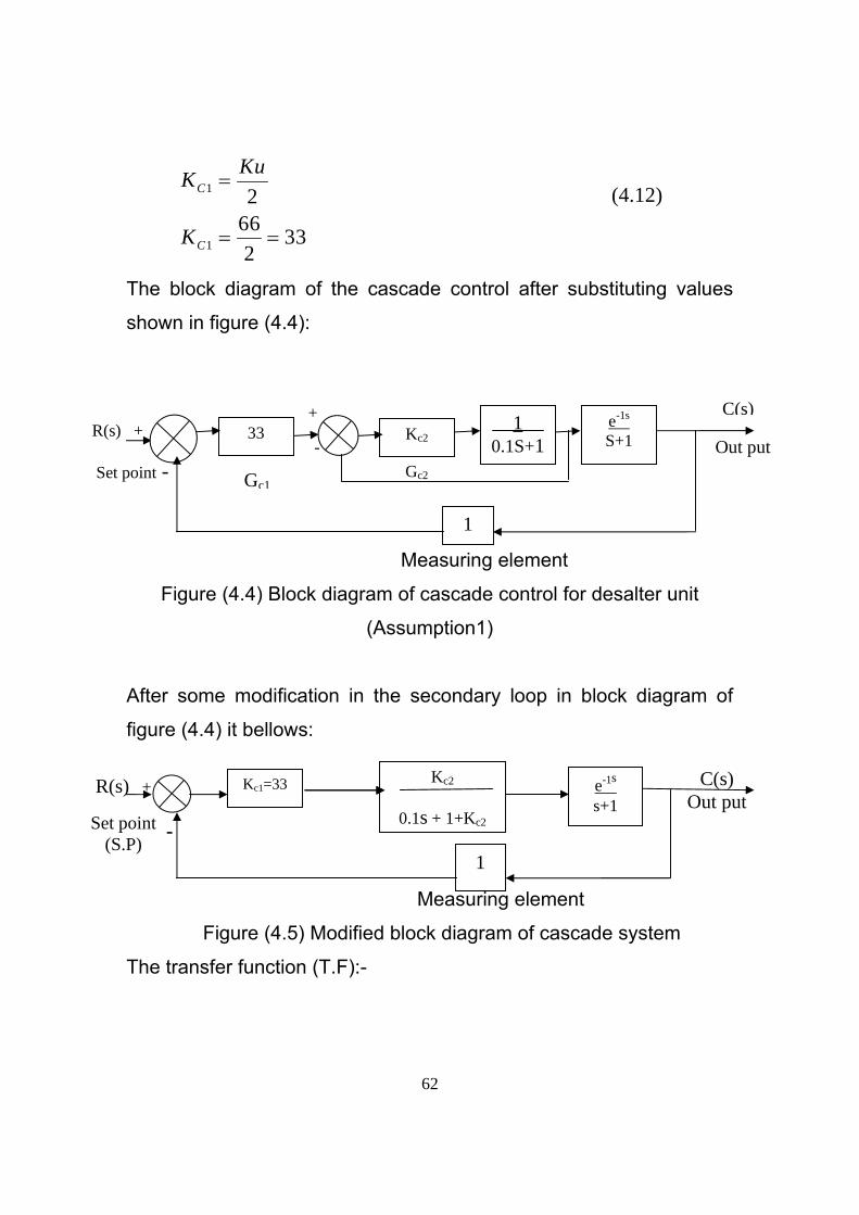
The block diagram of the cascade control after substituting values
shown in figure (4.4):
Measuring element
Figure (4.4) Block diagram of cascade control for desalter unit
(Assumption1)
After some modification in the secondary loop in block diagram of
figure (4.4) it bellows:
-
Measuring element
Figure (4.5) Modified block diagram of cascade system
The transfer function (T.F):-
e-1s S+1 33
1
R(s) +
Set point -
C(s)
Gc1
Kc2
Gc2
+
- 1
0.1S+1
e-1s s+1
Kc1=33
1
R(s) +
Set point (S.P)
C(s) Out put
Kc2
0.1s + 1+Kc2
Out put
(4.12)

63
( ). 1 ( )
F o rw a rdT Floop
Π=
+ Π
2
2
3 3 (1 0 .5 )( ) (0 .1 1 )( 1)(1 0 .5 )
C
c
K SF orw ardS K S S
−Π =
+ + + +
2
2
33 (1 0 .5 )( ) (0 .1 1 )( 1)(1 0 .5 )
C
c
K SLoopS K S S
−Π =
+ + + +
2( )
2 2
33 (1 0.5 )( ) ( ) (0.1 1 )( 1)(1 0.5 ) 33 (1 0.5 )
CS
c C
K SC SGR S S K S S K S
−= =
+ + + + + −
2( ) 3 2
2 2 2
33 (1 0.5 )( ) ( ) 0.05 (0.5 0.65) (1.6 15 ) 1 34
CS
C C C
K SC SGR S S K S K S K
−∴ = =
+ − + +
From the above transfer function, the characteristic equation is: 3 2
2 2 20.05 (0.65 0.5 ) (1.6 15 ) 1 34 0 C C CS K S K S K+ + + − + + = Using Routh criteria to get values of kc2:
Table (4.1) Routh Array for Cascade Control System
S3 0.05 1.6-15KC2
S2 0.65+ 0.5KC2 1+34KC2
S1 A1 0
S0 1+34KC2 0
In order for the system to be critically stable the first element in third
row A1 must be equal to zero and Kc = Ku. [2]
2 2 2 1
2
(0.65 0.5 )(1.6 15 ) 0.05(1 34 ) 0.65 0.5
C C C
C
K K KAK
+ − − +=
+
At critical stable A1 = 0 [2]
(4.13)
(4.14)
(4.15)
(4.16)
(4.17)
(4.18)
(4.19)
64
The equation will be: 2
2 22
2 2
7.5 10.42 0.99 0
1.38 0.132 0 C C
C C
K K
K K
+ − =
+ − =
And that leads Kc to have the following values:
Kc = + 1.47, Kc = -0.69
From the above values of Kc it can be see, that Routh criteria failed to
specify the ultimate gain because all values of Kc2 are less than value
of Kc1.
Quite often it will be not arbitrarily to select a very large kc2 but rather
select it in coordination with the resulting values of kc1. [1]
∴ Select Kc2 = 50
B. Assumption (2):
min1
min5.0min5
2
1
=
==
d
p
P
t
ττ
1
1
2
1 0 . 5 5 1. 5 1 1 0 . 5 5 5 1
1 0 . 5 1
s
P
P
eGS S
GS
− −∴ = =
+ + +
∴ =+
For using simple feedback control, the open – loop transfer function
with p – control is:
(4.20)
(4.20a)
(4.21)
(4.22)
65
1
1 2 1 1
1 2 1 1
1. . 0 .55 1 5 1
1 1 0 .5 1. . . 0 .5 1 1 0 .5 5 1
s
C P P C
C P P C
eG G G KS
SG G G KS S S
−
=+ +
−=
+ + +
The cross over frequency can be found from the equation that sets
the total phase lag equal to – 180o:
=φ = total phase lag = - 180o
1t a n pwϕ τ−= −
0 1 1
2
180 tan ( 0.5 ) ( ) tan ( 5 ) 11.14 / m in
1 ( )
P
P
w w ww rad
KARwτ
− −− = − + − + −∴ =
=+
1 2 2
1
1 1. . ( 0 . 5 ) 1 ( 5 ) 1
0 . 0 0 4
C
C
A R Kw w
A R K
=+ +
=
The ultimate value of the gain ku can be found when
AR= 1
1 = 0.004 ku
Ku = 250
From (Z-N) tuning technique the controller gain kc1 value is:
1
1
22 5 0 1 2 5
2
C
C
K uK
K
=
∴ = =
(4.23)
(4.24)
(4.10)[1]
(4.25)
(4.11)[1]
(4.26)
(4.26a)
(4.12)
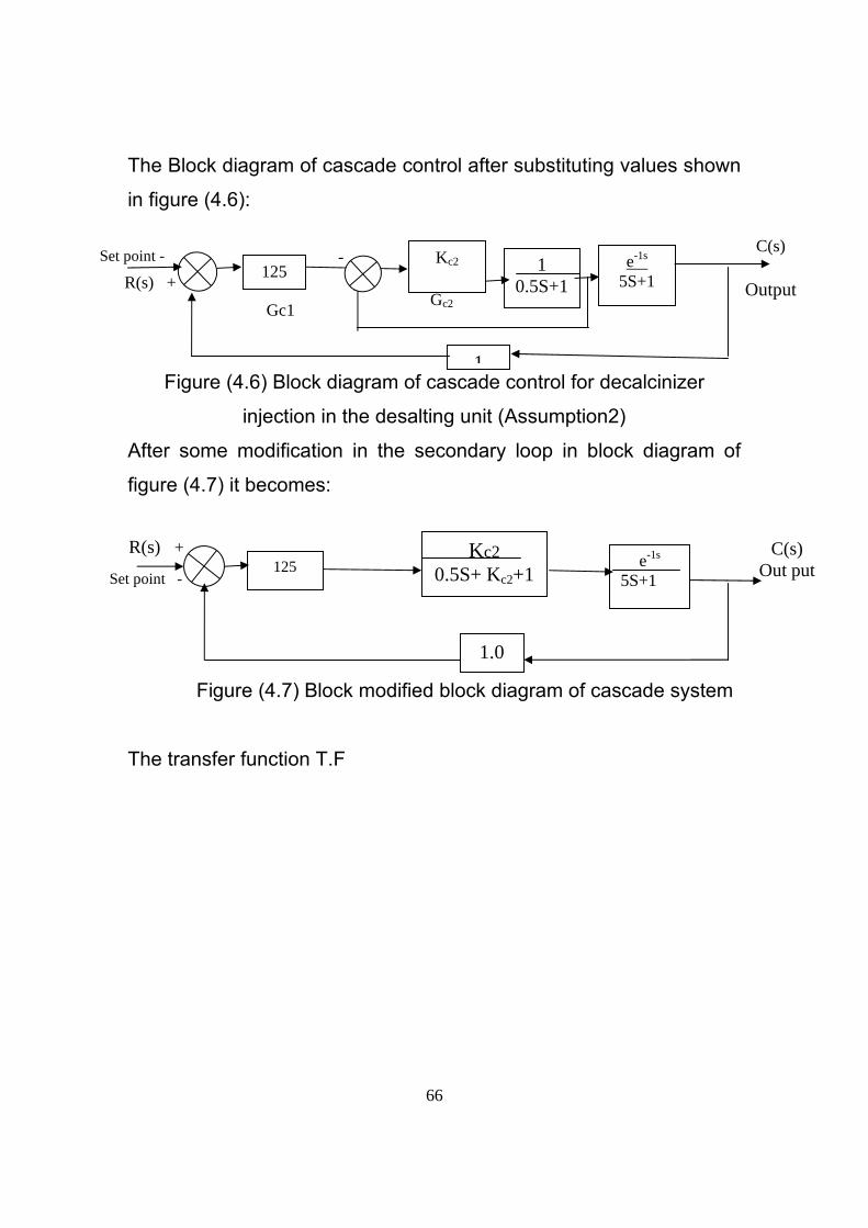
66
The Block diagram of cascade control after substituting values shown
in figure (4.6):
Figure (4.6) Block diagram of cascade control for decalcinizer
injection in the desalting unit (Assumption2)
After some modification in the secondary loop in block diagram of
figure (4.7) it becomes:
Figure (4.7) Block modified block diagram of cascade system
The transfer function T.F
Gc1
- Set point -
R(s) + Kc2 e-1s
5S+1
1
C(s)
Output Gc2
1 0.5S+1
e-1s 5S+1
125
1.0
R(s) +
Set point -
C(s) Out put
Kc2 0.5S+ Kc2+1
125
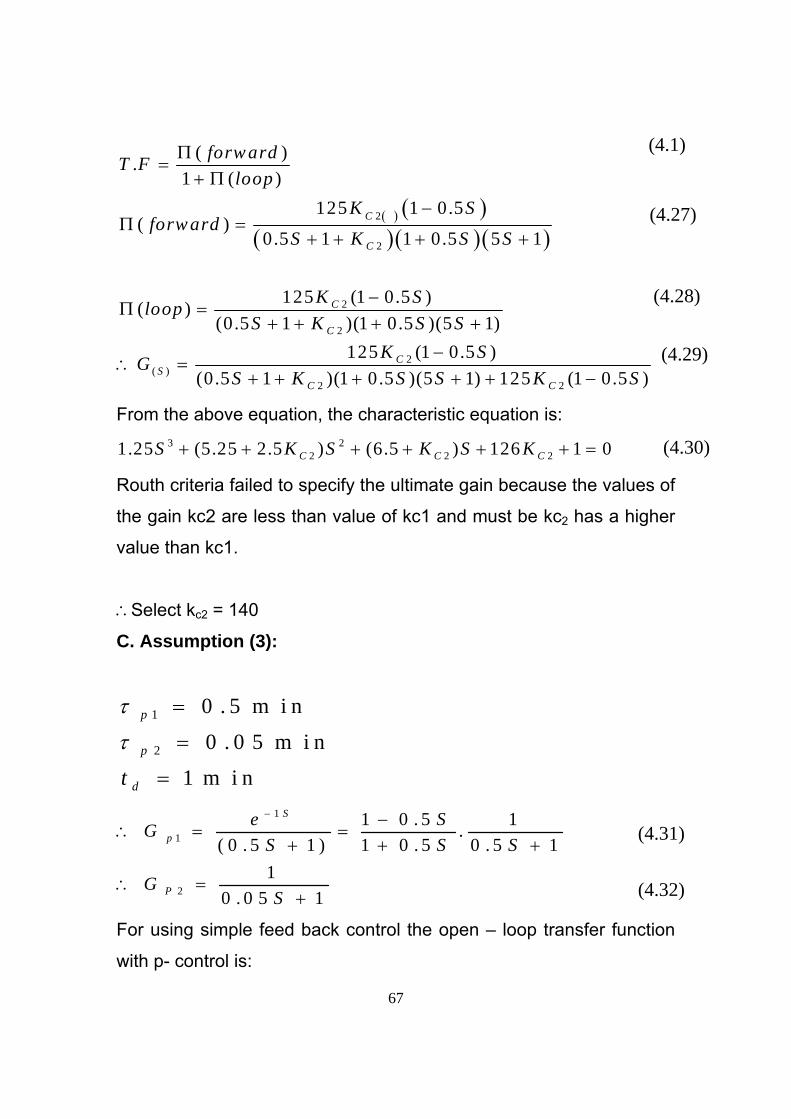
67
( ) ( )( )( )( )
2
2
2
2
( ). 1 ( )
125 1 0.5( )
0.5 1 1 0.5 5 1
125 (1 0.5 )( )(0.5 1 )(1
C
C
C
C
forwardT Floop
K Sforward
S K S S
K SloopS K
Π=
+ Π
−Π =
+ + + +
−Π =
+ + +
2( )
2 2
0.5 )(5 1)
125 (1 0.5 )(0.5 1 )(1 0.5 )(5 1) 125 (1 0.5 )
CS
C C
S SK SG
S K S S K S
+
−∴ =
+ + + + + −
From the above equation, the characteristic equation is:
3 22 2 21.25 (5.25 2.5 ) (6.5 ) 126 1 0 C C CS K S K S K+ + + + + + =
Routh criteria failed to specify the ultimate gain because the values of
the gain kc2 are less than value of kc1 and must be kc2 has a higher
value than kc1.
∴Select kc2 = 140
C. Assumption (3):
1
2
0 . 5 m i n
0 . 0 5 m i n
1 m i n
p
p
dt
τ
τ
=
=
=
1
1
2
1 0 . 5 1. ( 0 . 5 1 ) 1 0 . 5 0 . 5 1
1 0 . 0 5 1
S
p
P
e SGS S S
GS
− −∴ = =
+ + +
∴ =+
For using simple feed back control the open – loop transfer function
with p- control is:
(4.1)
(4.27)
(4.28)
(4.29)
(4.30)
(4.31)
(4.32)
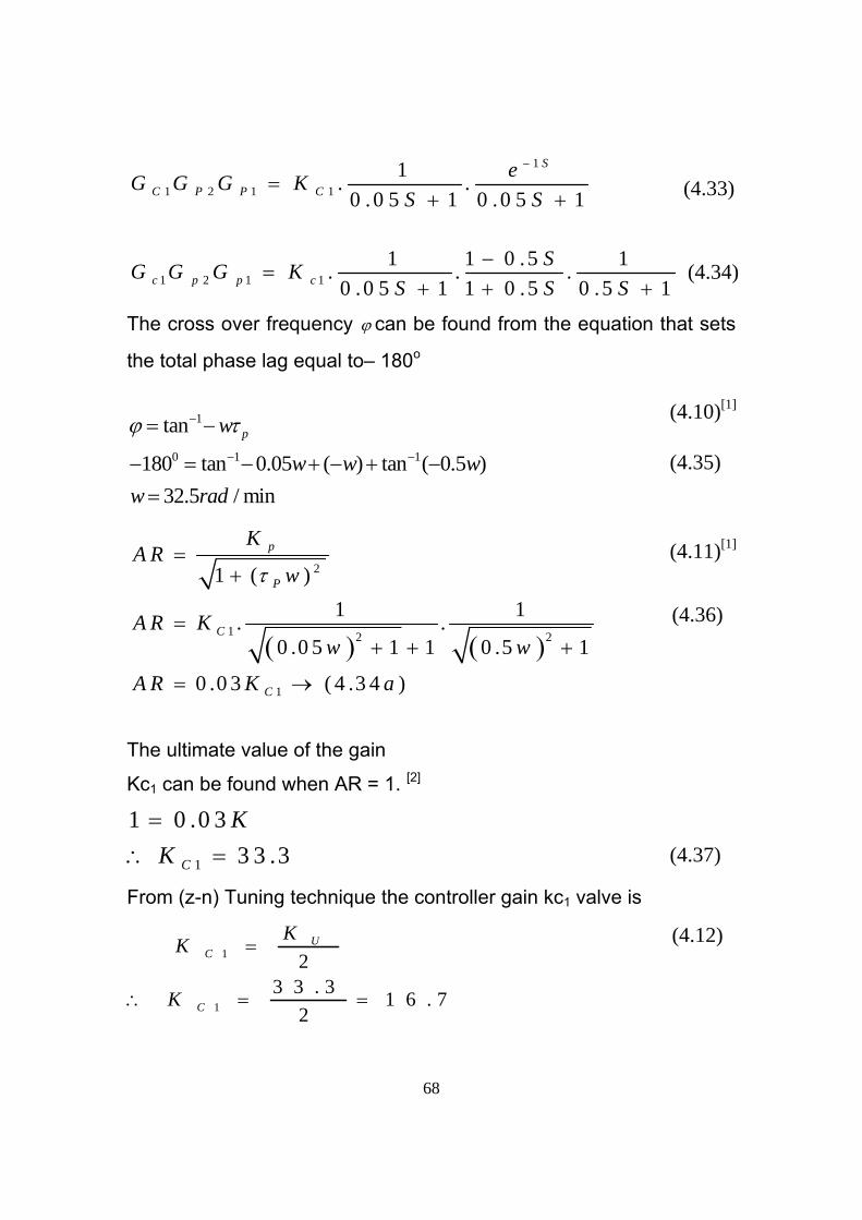
68
1
1 2 1 1
1 2 1 1
1. . (0 .0 5 1 0 .0 5 1
1 1 0 .5 1. . .0 .0 5 1 1 0 .5 0 .5 1
S
C P P C
c p p c
eG G G KS S
SG G G KS S S
−
=+ +
−=
+ + +
The cross over frequency ϕ can be found from the equation that sets
the total phase lag equal to– 180o
1
0 1 1
tan
180 tan 0.05 ( ) tan ( 0.5 ) pw
w w w
ϕ τ−
− −
= −
− = − + − + −32.5 / minw rad=
( ) ( )
2
1 2 2
1
1 ( )
1 1. . 0 .0 5 1 1 0 .5 1
0 .0 3 ( 4 .3 4 )
p
P
C
C
KA R
w
A R Kw w
A R K a
τ=
+
=+ + +
= →
The ultimate value of the gain
Kc1 can be found when AR = 1. [2]
1
1 0 .0 3 3 3 .3C
KK=
∴ =
From (z-n) Tuning technique the controller gain kc1 valve is
1
1
2
3 3 . 3 1 6 . 72
UC
C
KK
K
=
∴ = =
(4.33)
(4.34)
(4.10)[1]
(4.35)
(4.11)[1]
(4.36)
(4.37)
(4.12)
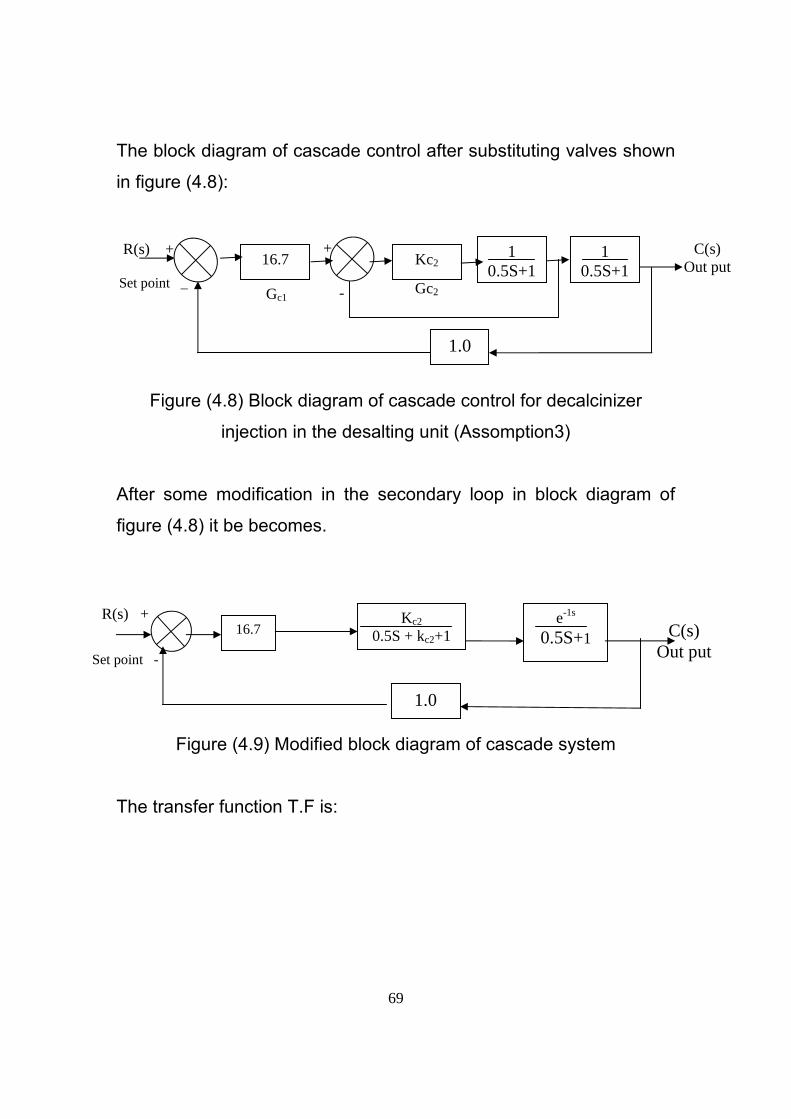
69
The block diagram of cascade control after substituting valves shown
in figure (4.8):
Figure (4.8) Block diagram of cascade control for decalcinizer
injection in the desalting unit (Assomption3)
After some modification in the secondary loop in block diagram of
figure (4.8) it be becomes.
Figure (4.9) Modified block diagram of cascade system
The transfer function T.F is:
1 0.5S+1
16.7
1.0
R(s) +
Set point _
C(s) Out put
Gc1
Kc2
Gc2
+
-
1 0.5S+1
e-1s 0.5S+1 16.7
1.0
R(s) +
Set point -
C(s) Out put
Kc2 0.5S + kc2+1
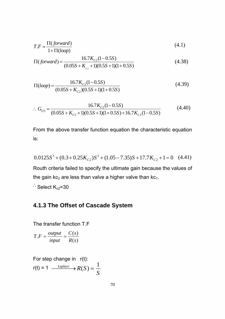
70
2
2
( ). 1 ( )
16.7 (1 0.5 )( ) (0.05 1)(0.5 1)(1 0.5 )
C
C
forwardT Floop
K SforwardS K S S
Π=
+Π−
Π =+ + + +
2
2
2( )
2 2
16.7 (1 0.5 )( ) (0.05 )(0.5 1)(1 0.5 )
16.7 (1 0.5 ) (0.05 1)(0.5 1)(1 0.5 ) 16.7 (1 0.5 )
C
C
CS
C C
K SloopS K S S
K SGS K S S K S
−Π =
+ + +
−∴ =
+ + + + + −
From the above transfer function equation the characteristic equation
is:
3 2
2 20.0125 (0.3 0.25 ) (1.05 7.35) 17.7 1 0 C CS K S S K+ + + − + + =
Routh criteria failed to specify the ultimate gain because the values of
the gain kc2 are less than valve a higher valve than kc1. ∴Select Kc2=30
4.1.3 The Offset of Cascade System
The transfer function T.F
)()(.
sRsC
inputoutputFT ==
For step change in r(t):
r(t) = 1 S
SRLaplace 1)( =⎯⎯ →⎯
(4.1)
(4.38)
(4.39)
(4.40)
(4.41)
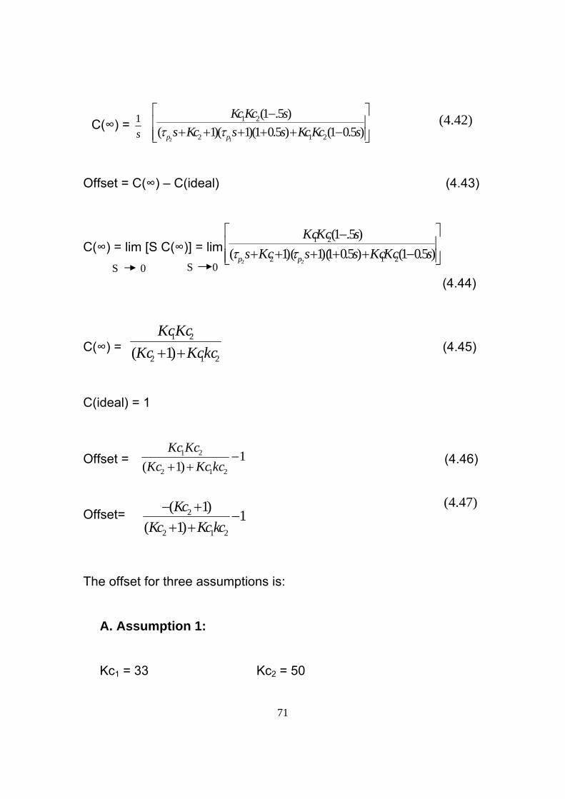
71
C(∞) = s1
2 1
1 2
2 1 2
(1 .5 ) ( 1)( 1)(1 0.5 ) (1 0.5 )p p
KcKc ss Kc s s KcKc sτ τ
⎡ ⎤−⎢ ⎥
+ + + + + −⎢ ⎥⎣ ⎦
Offset = C(∞) – C(ideal) (4.43)
C(∞) = lim [S C(∞)] = lim⎥⎥⎦
⎤
⎢⎢⎣
⎡
−+++++−
)5.01()5.01)(1)(1()5.1(
212
21
22sKcKcssKcs
sKcKc
pp ττ
(4.44)
C(∞) = 212
21
)1( kcKcKcKcKc++ (4.45)
C(ideal) = 1
Offset = 1)1( 212
21 −++ kcKcKcKcKc
(4.46)
Offset=
The offset for three assumptions is:
A. Assumption 1:
Kc1 = 33 Kc2 = 50
2
2 1 2
( 1) 1 ( 1)
KcKc Kckc− +
−+ +
S 0 S 0
(4.42)
(4.47)
72
∴ Offset = 03.0)33)(50(51
51)1(
)1(
212
2 −=+−
=+++−
kcKcKcKc
B. Assumption 2: Kc1 = 125 Kc2 = 140
∴ Offset = 008.0)125)(140()1140(
)1140(−=
+++−
C. Assumption 3: Kc1= 16.7 Kc2 = 30
∴Offset = 058.0)7.16)(30()130(
)130(−=
+++
4.2 Feedback Control Strategy
Consider the composition control system for decalcinizer addition in
a desalting unit figure (4.10). As shown in figure (4.10) below, the
feed back control system contains one process.
This process is the removal of calcium from crude oil in the desalter
and the controlled output is the concentration of calcium in desalted
crude C1.
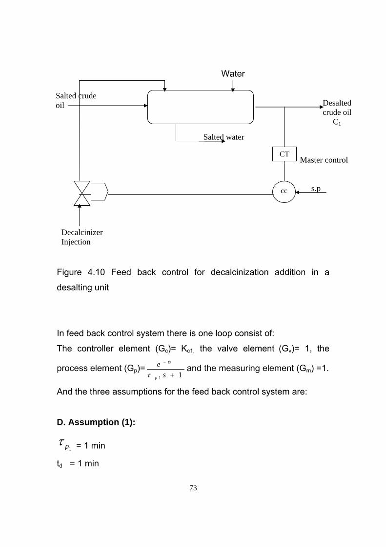
73
Water
Figure 4.10 Feed back control for decalcinization addition in a
desalting unit
In feed back control system there is one loop consist of:
The controller element (Gc)= Kc1, the valve element (Gv)= 1, the
process element (Gp)= 11 +
−
se
p
ts
τand the measuring element (Gm) =1.
And the three assumptions for the feed back control system are:
D. Assumption (1):
1pτ = 1 min
td = 1 min
cc
CT
Salted crude oil Desalted
crude oil C1
Salted water
s.p
Decalcinizer Injection
Master control
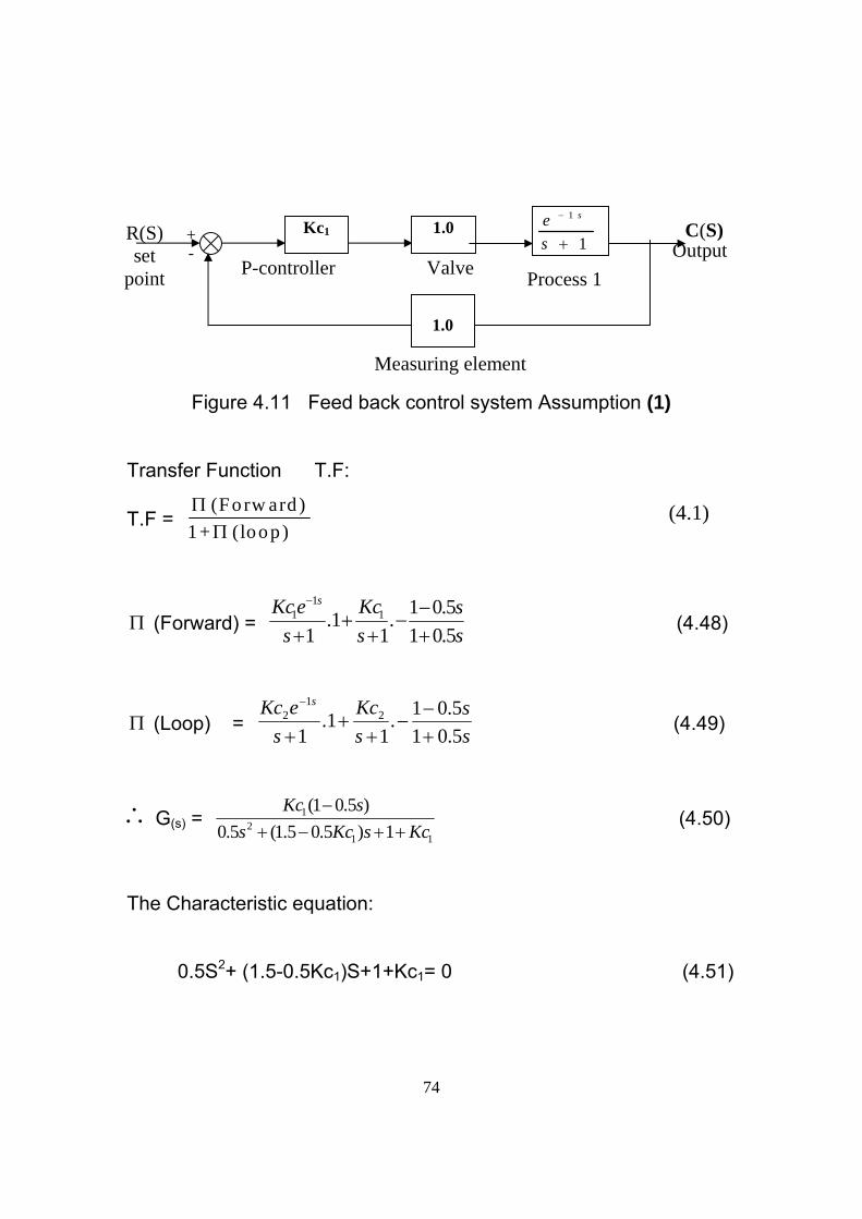
74
Figure 4.11 Feed back control system Assumption (1)
Transfer Function T.F:
T.F = (Forw ard )
1+ (loop) Π
Π
Π (Forward) = ss
sKc
seKc s
5.015.01.
11.
11
11
+−
−+
++
−
(4.48)
Π (Loop) = ss
sKc
seKc s
5.015.01.
11.
12
12
+−
−+
++
−
(4.49)
∴G(s) = 11
21
1)5.05.1(5.0)5.01(
KcsKcssKc
++−+−
(4.50)
The Characteristic equation:
0.5S2+ (1.5-0.5Kc1)S+1+Kc1= 0 (4.51)
Measuring element
Process 1
Kc1 1.0 1
1
+
−
se s
1.0
Valve
R(S) set
point
Output
P-controller
+ -
C(S)
(4.1)
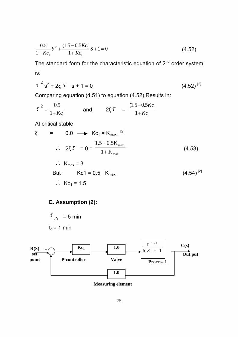
75
011
5.05.1(1
5.0
1
12
1
=++−
++
SKc
KcSKc (4.52)
The standard form for the characteristic equation of 2nd order system
is:
2τ s2 + 2ξ τ s + 1 = 0 (4.52) [2]
Comparing equation (4.51) to equation (4.52) Results in:
2τ = 11
5.0Kc+ and 2ξτ =
1
1
15.05.1(
KcKc
+−
At critical stable
ξ = 0.0 Kc1 = Kmax . [2]
∴ 2ξτ = 0 = max
max
K1K5.05.1
+
− (4.53)
∴Kmax = 3
But Kc1 = 0.5 Kmax. (4.54) [2]
∴Kc1 = 1.5
E. Assumption (2):
1pτ = 5 min
td = 1 min
Measuring element
Process 1
Kc1 1.0 1
5 1
seS
−
+
1.0
Valve
R(S) set
point Out put
P-controller
+
C(s)
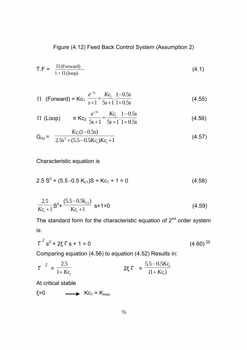
76
Figure (4.12) Feed Back Control System (Assumption 2)
T.F = (loop)+1
(Forward)Π
Π (4.1)
Π (Forward) = Kc1 ss
sKc
se s
5.015.01.
1511
1
+−
+=
+
−
(4.55)
Π (Loop) = Kc2 ss
sKc
se s
5.015.01.
15151
1
+−
+=
+
−
(4.56)
G(s) = 1)5.05.5(5.2)5.01(
112
1
+−+−
KcKcssKc
(4.57)
Characteristic equation is
2.5 S2 + (5.5 -0.5 Kc1)S + Kc1 + 1 = 0 (4.58)
15.2
1 +Kc S2+ 1)5.05.5(
1
1
+−
KckC s+1=0 (4.59)
The standard form for the characteristic equation of 2nd order system
is: 2τ s2 + 2ξτ s + 1 = 0 (4.60) [2]
Comparing equation (4.56) to equation (4.52) Results in:
2τ = 11
5.2Kc+ 2ξτ = )1(
5.05.5
1
1
KcKc
+−
At critical stable
ξ=0 Kc1 = Kmax
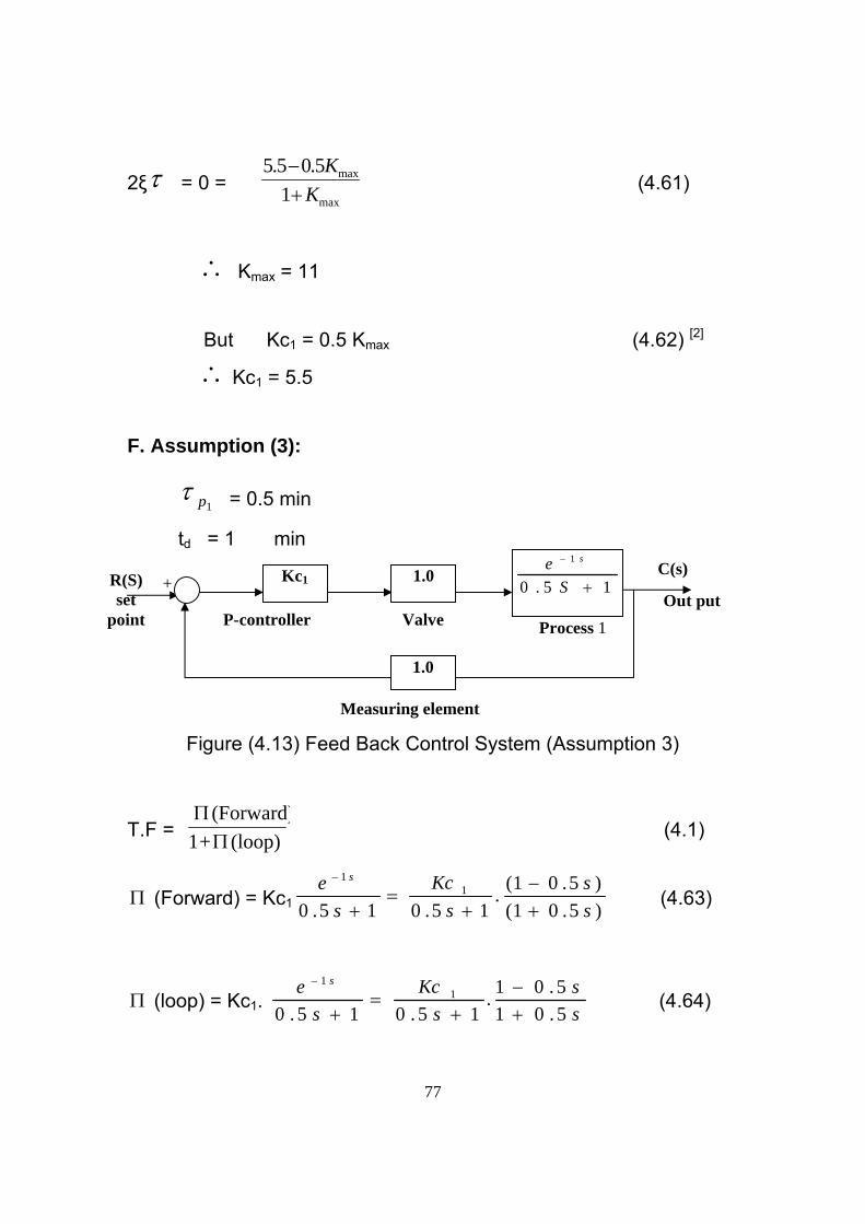
77
2ξτ = 0 = max
max
15.05.5
KK
+−
(4.61)
∴ Kmax = 11
But Kc1 = 0.5 Kmax (4.62) [2]
∴Kc1 = 5.5
F. Assumption (3):
1pτ = 0.5 min
td = 1 min
Figure (4.13) Feed Back Control System (Assumption 3)
T.F = (loop) + 1(Forward) Π
Π (4.1)
Π (Forward) = Kc1 )5.01()5.01(.
15.015.01
1
ss
sKc
se s
+−
+=
+
−
(4.63)
Π (loop) = Kc1. ss
sKc
se s
5.015.01.
15.015.01
1
+−
+=
+
−
(4.64)
Measuring element
Process 1
Kc1 1.0 1
0 . 5 1
seS
−
+
1.0
Valve
R(S) set
point Out put
P-controller
+
C(s)
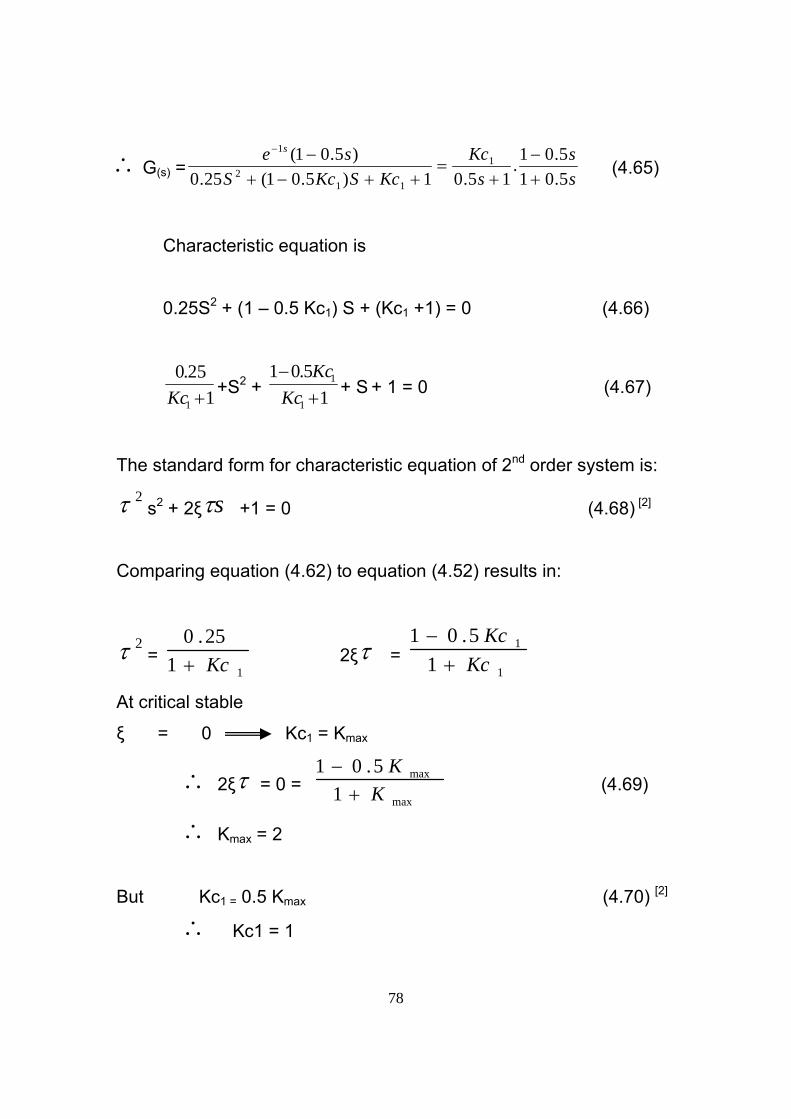
78
∴G(s) = ss
sKc
KcSKcSse s
5.015.01.
15.01)5.01(25.0)5.01( 1
112
1
+−
+=
++−+−−
(4.65)
Characteristic equation is
0.25S2 + (1 – 0.5 Kc1) S + (Kc1 +1) = 0 (4.66)
125.0
1 +Kc +S2 + 15.01
1
1
+−Kc
Kc+ S + 1 = 0 (4.67)
The standard form for characteristic equation of 2nd order system is: 2τ s2 + 2ξ sτ +1 = 0 (4.68) [2]
Comparing equation (4.62) to equation (4.52) results in:
2τ = 11
25.0Kc+ 2ξτ =
1
1
15.01Kc
Kc+
−
At critical stable
ξ = 0 Kc1 = Kmax
∴ 2ξτ = 0 = max
max
15.01K
K+
− (4.69)
∴ Kmax = 2
But Kc1 = 0.5 Kmax (4.70) [2]
∴ Kc1 = 1
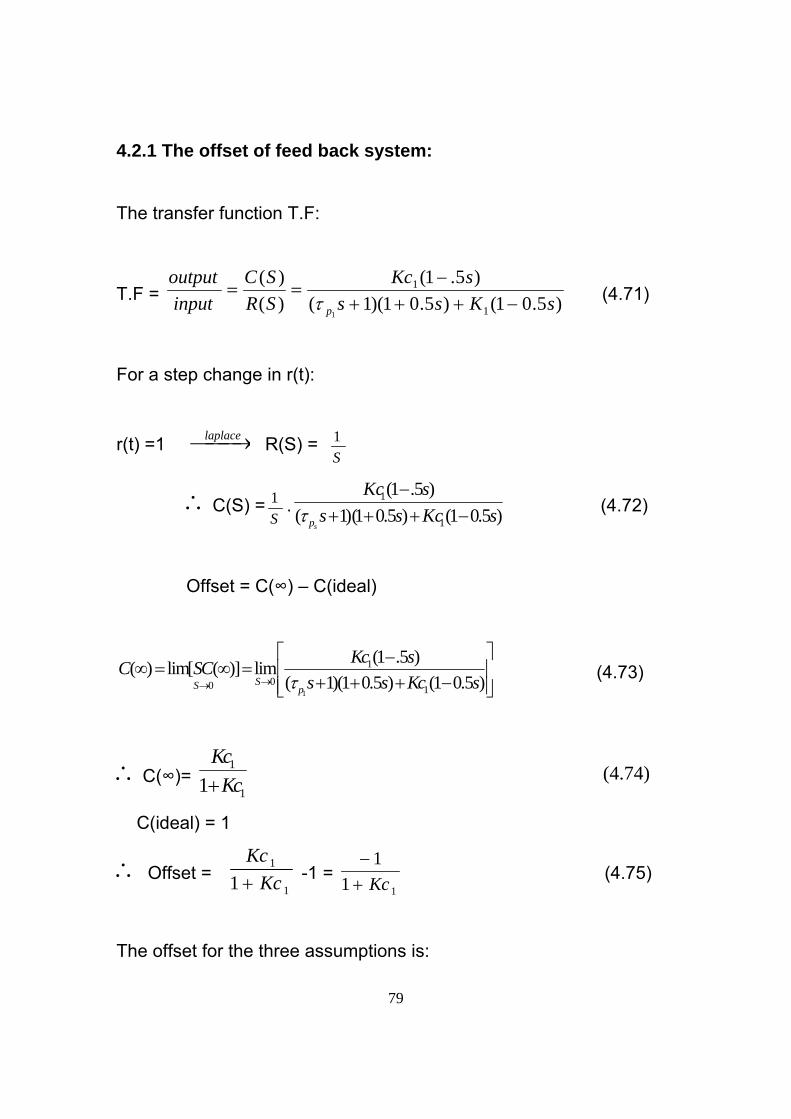
79
4.2.1 The offset of feed back system: The transfer function T.F:
T.F = )5.01()5.01)(1()5.1(
)()(
1
1
1sKss
sKcSRSC
inputoutput
p −+++−
==τ (4.71)
For a step change in r(t):
r(t) =1 ⎯⎯→⎯laplace R(S) = S1
∴C(S) =S1 . )5.01()5.01)(1(
)5.1(
1
1
sKcsssKc
sp −+++−
τ (4.72)
Offset = C(∞) – C(ideal)
1
1
00 1
(1 .5 )( ) lim[ ( )] lim( 1)(1 0.5 ) (1 0.5 )SS p
Kc sC SCs s Kc sτ→→
⎡ ⎤−∞ = ∞ = ⎢ ⎥
+ + + −⎢ ⎥⎣ ⎦ (4.73)
∴C(∞)= 1
1
1
KcKc+
C(ideal) = 1
∴ Offset = 1
1
1 KcKc+ -1 =
111Kc+−
(4.75)
The offset for the three assumptions is:
(4.74)
80
D. Assumption (1): Kc1= 1.5
∴ Offset = 5.01
1+− = -0.4
E. Assumption (2): Kc1=5.5
∴Offset = 5.51
1+−
= -0.154
F. Assumption (3): Kc1= 1
∴Offset = 11
1+− = -0.5
81
4.3 Stability Analysis of the Control System A very important characteristic of transient performance of system is
its stability. It is required for the control system to keep the controlled
variables with in specified limits.
There are several methods to check whether a system is stable or
not, these are:
4.3.1 Bode Criterion A feed back control system is stable according to bode criterion if the
amplitude ratio of the corresponding open-loop transfer function is
less than one at the crossover frequency.
The crossover frequency is the frequency where the phase lag is
equal to (- 180 )˚ .
4.3.2 Nyguist stability criterion
It states that if the open-loop Nyguist plot of feedback system
encircles the point (- 1.0) as the frequency w takes any value from
(-∞ to +∞).
4.3.3 Root locus criterion: This criterion of stability does not require calculations of the actual
values of the roots of the characteristic equation, it only requires
82
whether any other roots lies to the right of the imaging axis (i.e., have
positive real part) that leads to unstable system.
4.4 Stability Analysis of Cascade Control System
The transfer function of cascade control system according to
assumption (1) was:
23 2
2 2 2
33 (1 0.5 )( ). ( ) 0.05 (0.5 0.65) (1.6 15 ) 1 34
C
C C C
K SC ST FR S S K S K S K
−∴ = =
+ − + +
Select Kc2 = 50.
4.4.1 Bode criterion:
The bode plot of the cascade transfer function is plotted using
MATLAB as shown in figure (4.14):
(4.17)
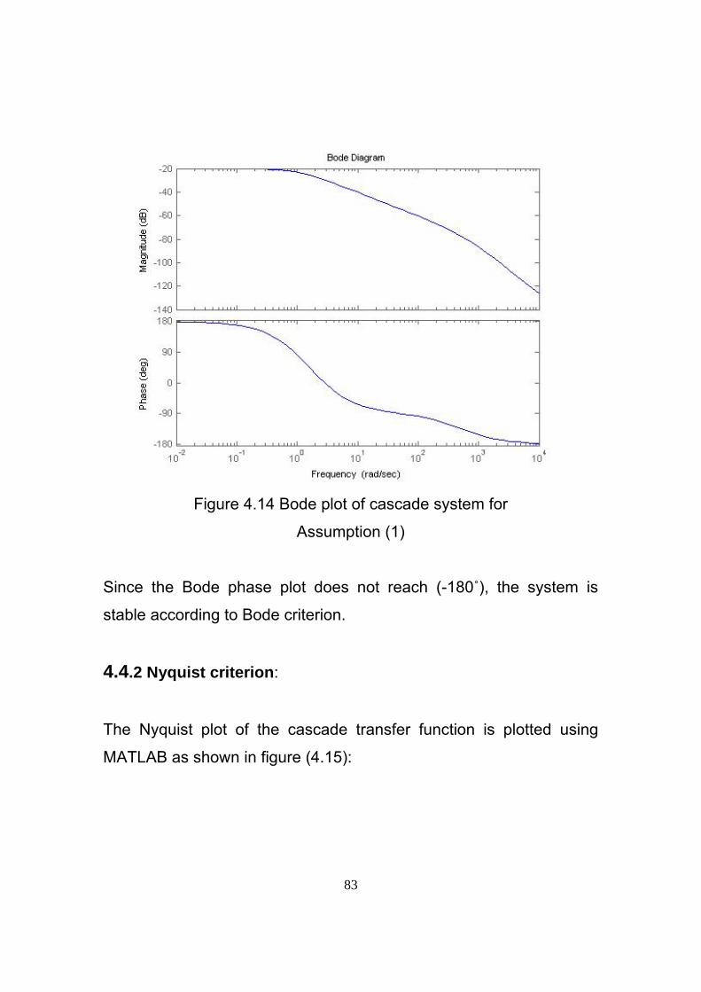
83
Figure 4.14 Bode plot of cascade system for
Assumption (1)
Since the Bode phase plot does not reach (-180˚), the system is
stable according to Bode criterion.
4.4.2 Nyquist criterion:
The Nyquist plot of the cascade transfer function is plotted using
MATLAB as shown in figure (4.15):
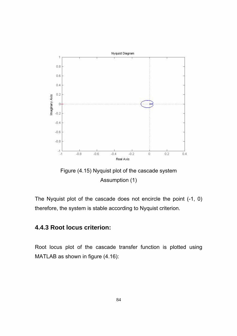
84
Figure (4.15) Nyquist plot of the cascade system
Assumption (1)
The Nyquist plot of the cascade does not encircle the point (-1, 0)
therefore, the system is stable according to Nyquist criterion.
4.4.3 Root locus criterion:
Root locus plot of the cascade transfer function is plotted using
MATLAB as shown in figure (4.16):
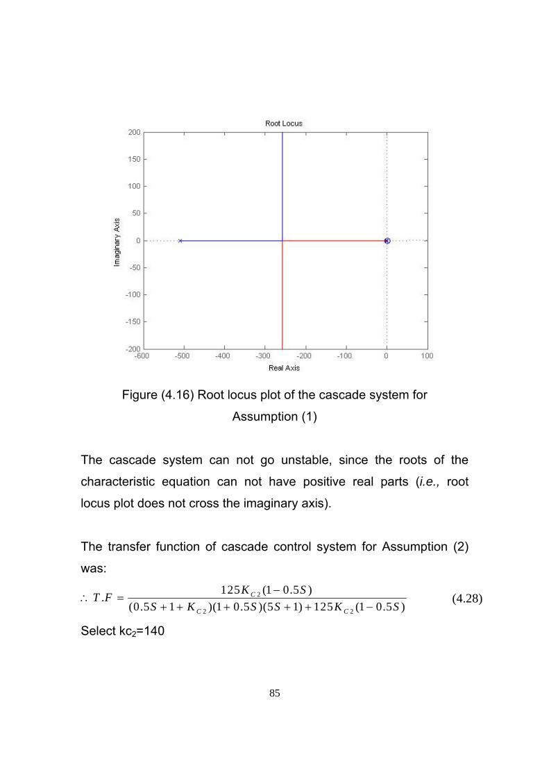
85
Figure (4.16) Root locus plot of the cascade system for
Assumption (1)
The cascade system can not go unstable, since the roots of the
characteristic equation can not have positive real parts (i.e., root
locus plot does not cross the imaginary axis).
The transfer function of cascade control system for Assumption (2)
was:
2
2 2
125 (1 0.5 ). (0.5 1 )(1 0.5 )(5 1) 125 (1 0.5 )
C
C C
K ST FS K S S K S
−∴ =
+ + + + + −
Select kc2=140
(4.28)
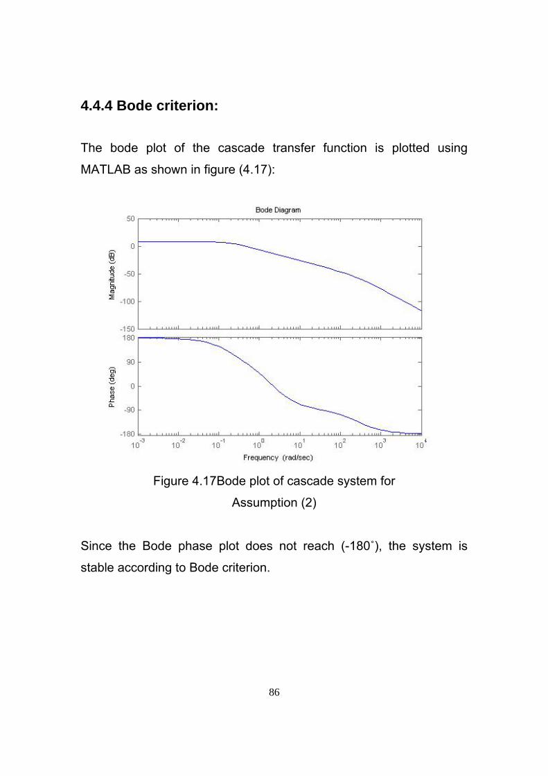
86
4.4.4 Bode criterion:
The bode plot of the cascade transfer function is plotted using
MATLAB as shown in figure (4.17):
Figure 4.17Bode plot of cascade system for
Assumption (2)
Since the Bode phase plot does not reach (-180˚), the system is
stable according to Bode criterion.
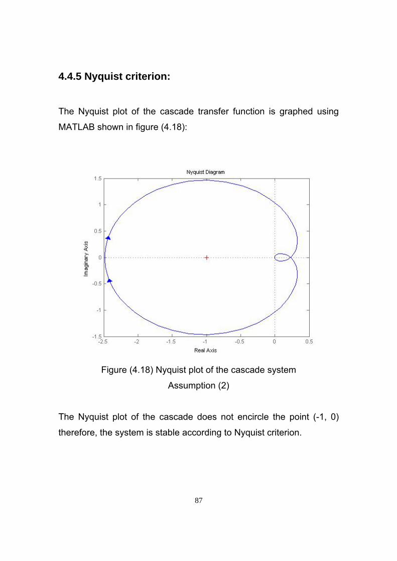
87
4.4.5 Nyquist criterion: The Nyquist plot of the cascade transfer function is graphed using
MATLAB shown in figure (4.18):
Figure (4.18) Nyquist plot of the cascade system
Assumption (2)
The Nyquist plot of the cascade does not encircle the point (-1, 0)
therefore, the system is stable according to Nyquist criterion.
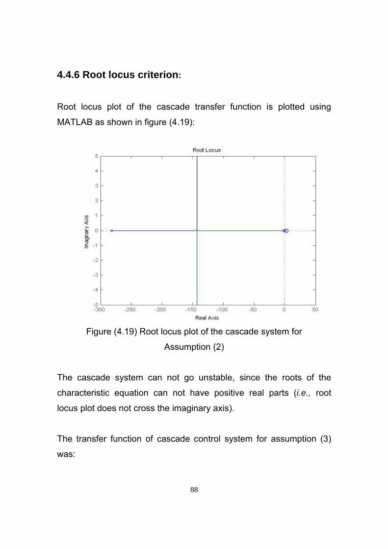
88
4.4.6 Root locus criterion:
Root locus plot of the cascade transfer function is plotted using
MATLAB as shown in figure (4.19):
Figure (4.19) Root locus plot of the cascade system for
Assumption (2)
The cascade system can not go unstable, since the roots of the
characteristic equation can not have positive real parts (i.e., root
locus plot does not cross the imaginary axis).
The transfer function of cascade control system for assumption (3)
was:
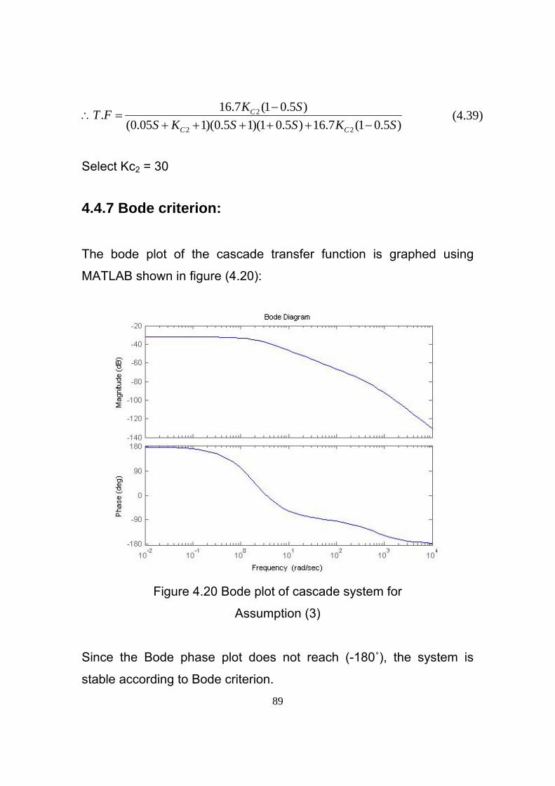
89
2
2 2
16.7 (1 0.5 ). (0.05 1)(0.5 1)(1 0.5 ) 16.7 (1 0.5 )
C
C C
K ST FS K S S K S
−∴ =
+ + + + + −
Select Kc2 = 30
4.4.7 Bode criterion:
The bode plot of the cascade transfer function is graphed using
MATLAB shown in figure (4.20):
Figure 4.20 Bode plot of cascade system for
Assumption (3)
Since the Bode phase plot does not reach (-180˚), the system is
stable according to Bode criterion.
(4.39)
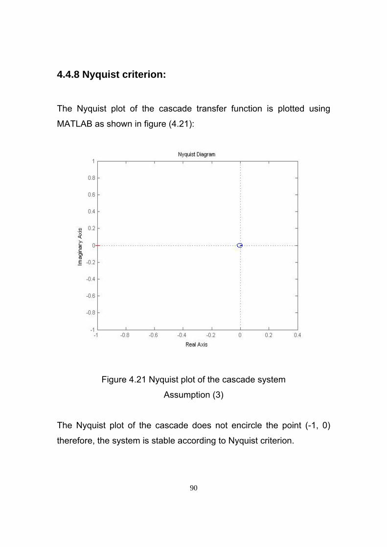
90
4.4.8 Nyquist criterion: The Nyquist plot of the cascade transfer function is plotted using
MATLAB as shown in figure (4.21):
Figure 4.21 Nyquist plot of the cascade system
Assumption (3)
The Nyquist plot of the cascade does not encircle the point (-1, 0)
therefore, the system is stable according to Nyquist criterion.
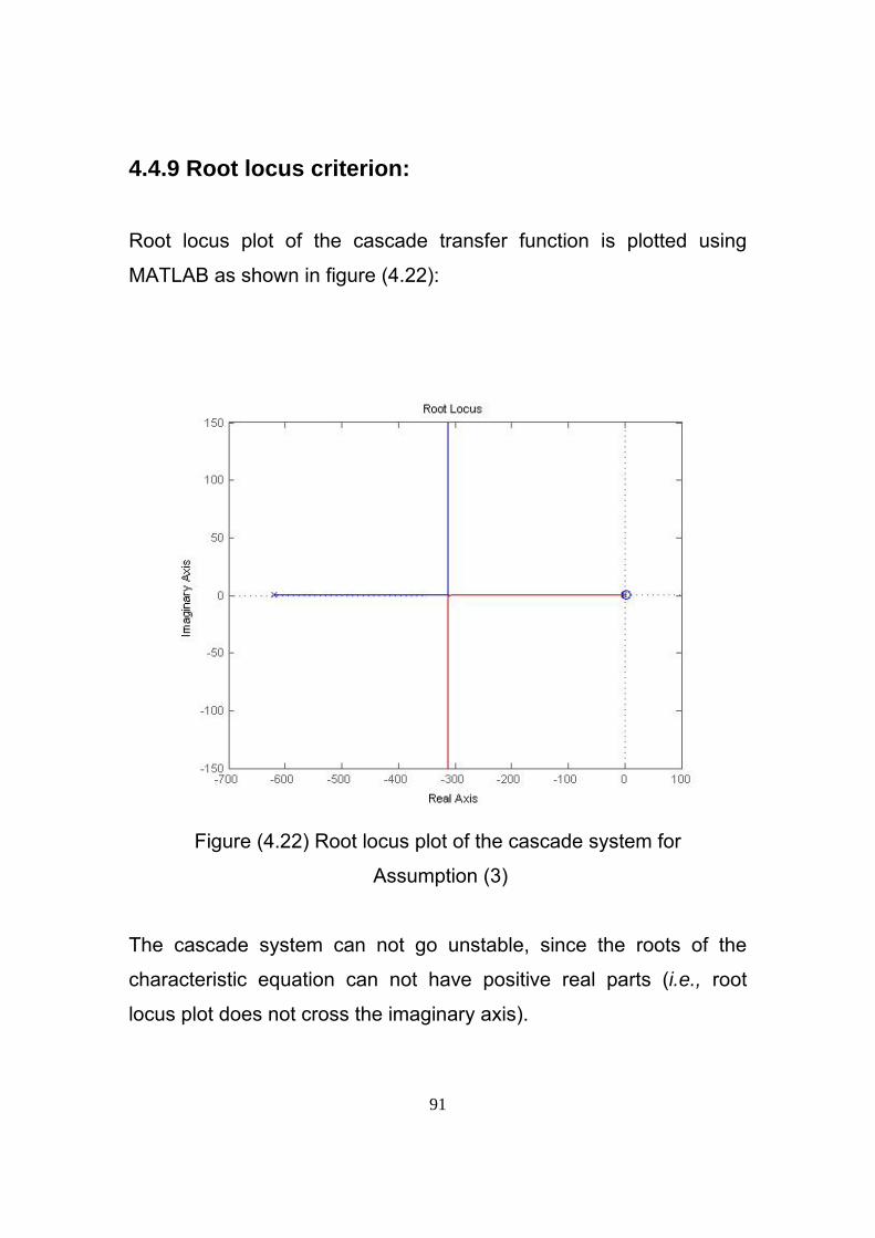
91
4.4.9 Root locus criterion:
Root locus plot of the cascade transfer function is plotted using
MATLAB as shown in figure (4.22):
Figure (4.22) Root locus plot of the cascade system for
Assumption (3)
The cascade system can not go unstable, since the roots of the
characteristic equation can not have positive real parts (i.e., root
locus plot does not cross the imaginary axis).
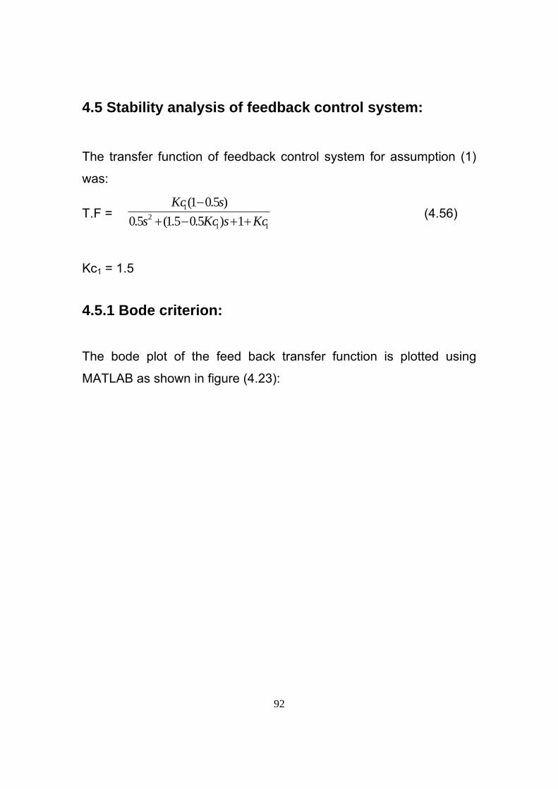
92
4.5 Stability analysis of feedback control system: The transfer function of feedback control system for assumption (1)
was:
T.F = 11
21
1)5.05.1(5.0)5.01(
KcsKcssKc
++−+−
(4.56)
Kc1 = 1.5
4.5.1 Bode criterion:
The bode plot of the feed back transfer function is plotted using
MATLAB as shown in figure (4.23):
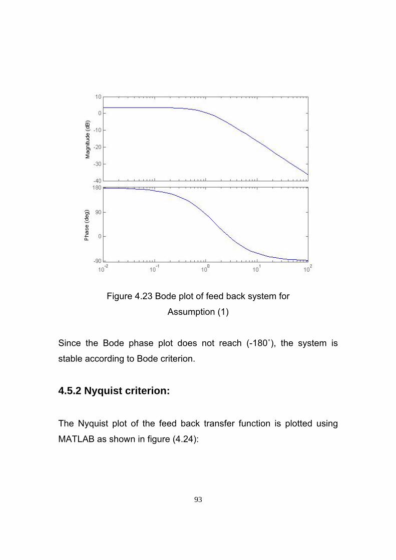
93
Figure 4.23 Bode plot of feed back system for
Assumption (1)
Since the Bode phase plot does not reach (-180˚), the system is
stable according to Bode criterion.
4.5.2 Nyquist criterion:
The Nyquist plot of the feed back transfer function is plotted using
MATLAB as shown in figure (4.24):
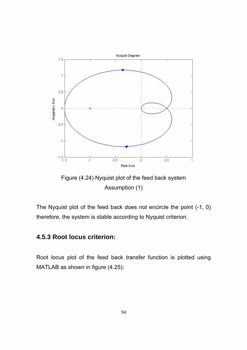
94
Figure (4.24) Nyquist plot of the feed back system
Assumption (1)
The Nyquist plot of the feed back does not encircle the point (-1, 0)
therefore, the system is stable according to Nyquist criterion.
4.5.3 Root locus criterion:
Root locus plot of the feed back transfer function is plotted using
MATLAB as shown in figure (4.25):
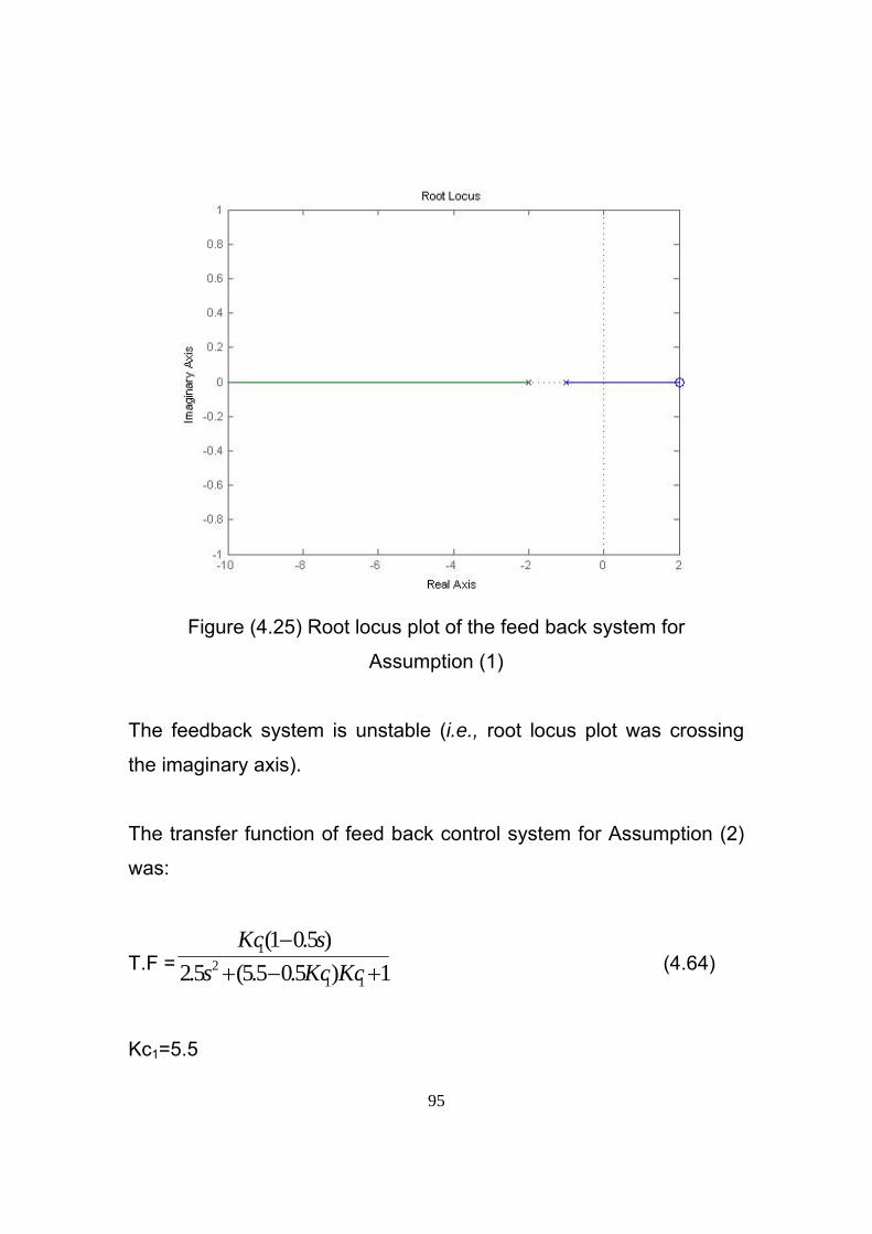
95
Figure (4.25) Root locus plot of the feed back system for
Assumption (1)
The feedback system is unstable (i.e., root locus plot was crossing
the imaginary axis).
The transfer function of feed back control system for Assumption (2)
was:
T.F = 1)5.05.5(5.2)5.01(
112
1
+−+−
KcKcssKc
(4.64)
Kc1=5.5
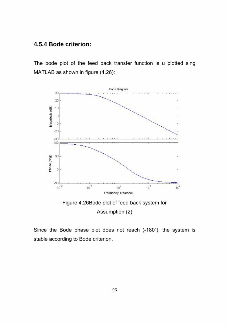
96
4.5.4 Bode criterion:
The bode plot of the feed back transfer function is u plotted sing
MATLAB as shown in figure (4.26):
Figure 4.26Bode plot of feed back system for
Assumption (2)
Since the Bode phase plot does not reach (-180˚), the system is
stable according to Bode criterion.
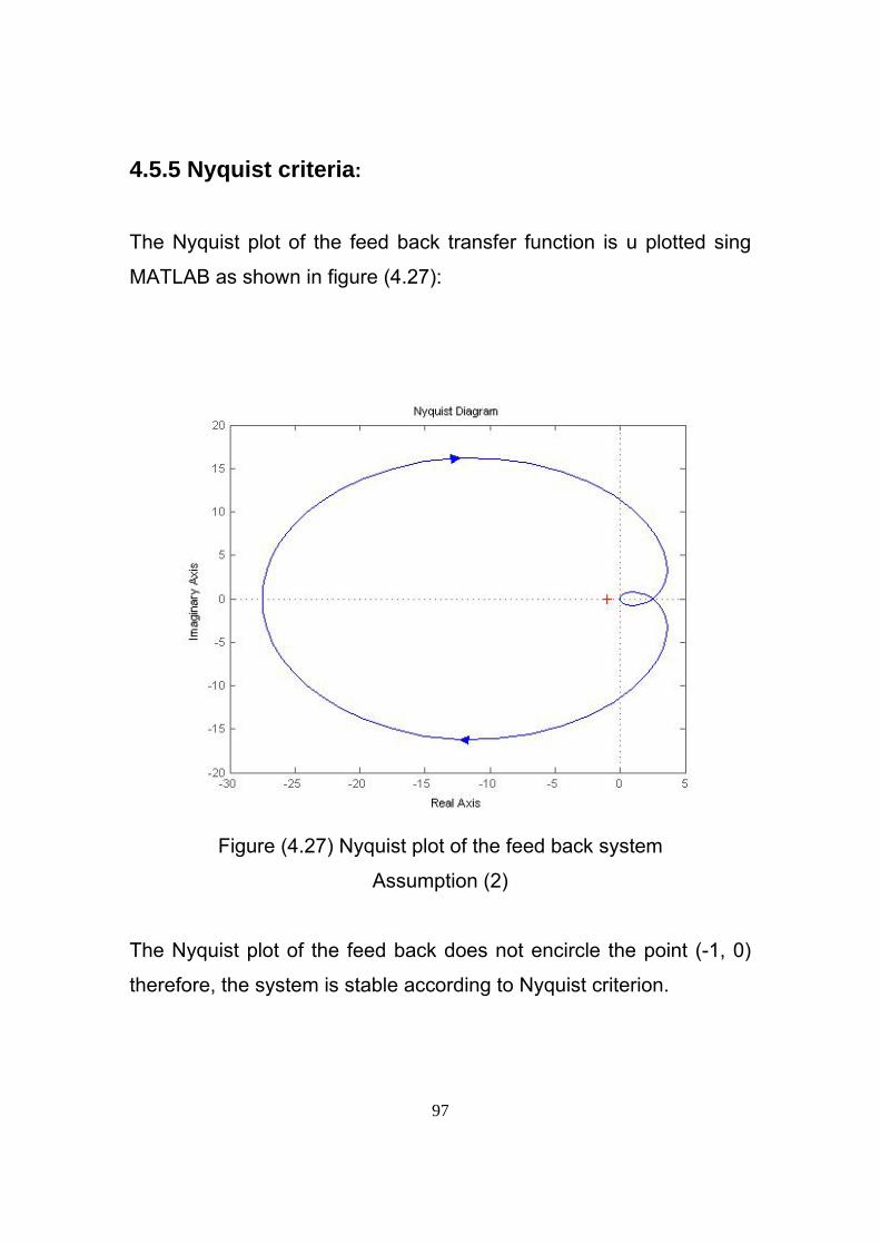
97
4.5.5 Nyquist criteria:
The Nyquist plot of the feed back transfer function is u plotted sing
MATLAB as shown in figure (4.27):
Figure (4.27) Nyquist plot of the feed back system
Assumption (2)
The Nyquist plot of the feed back does not encircle the point (-1, 0)
therefore, the system is stable according to Nyquist criterion.
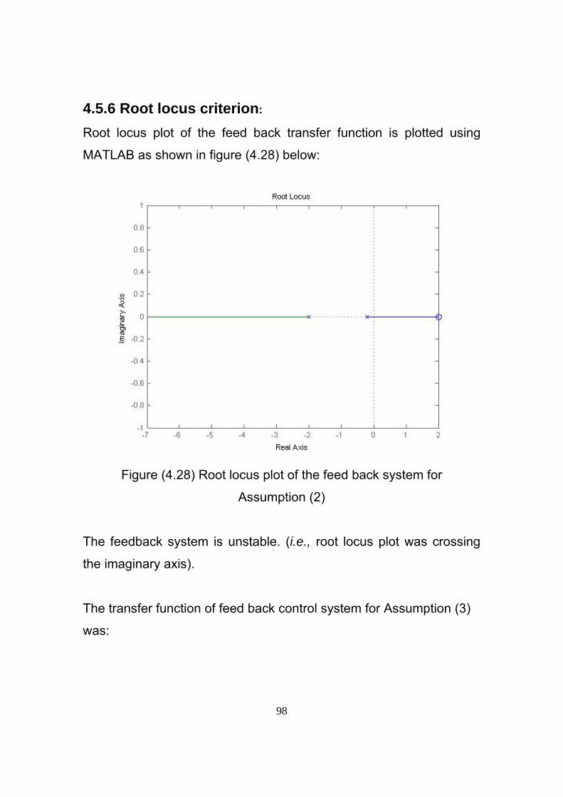
98
4.5.6 Root locus criterion:
Root locus plot of the feed back transfer function is plotted using
MATLAB as shown in figure (4.28) below:
Figure (4.28) Root locus plot of the feed back system for
Assumption (2)
The feedback system is unstable. (i.e., root locus plot was crossing
the imaginary axis).
The transfer function of feed back control system for Assumption (3)
was:
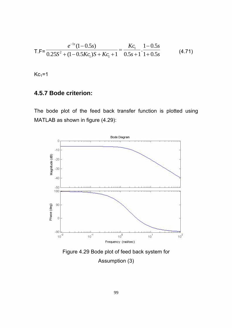
99
T.F= ss
sKc
KcSKcSse s
5.015.01.
15.01)5.01(25.0)5.01( 1
112
1
+−
+=
++−+−−
(4.71)
Kc1=1
4.5.7 Bode criterion:
The bode plot of the feed back transfer function is plotted using
MATLAB as shown in figure (4.29):
Figure 4.29 Bode plot of feed back system for
Assumption (3)
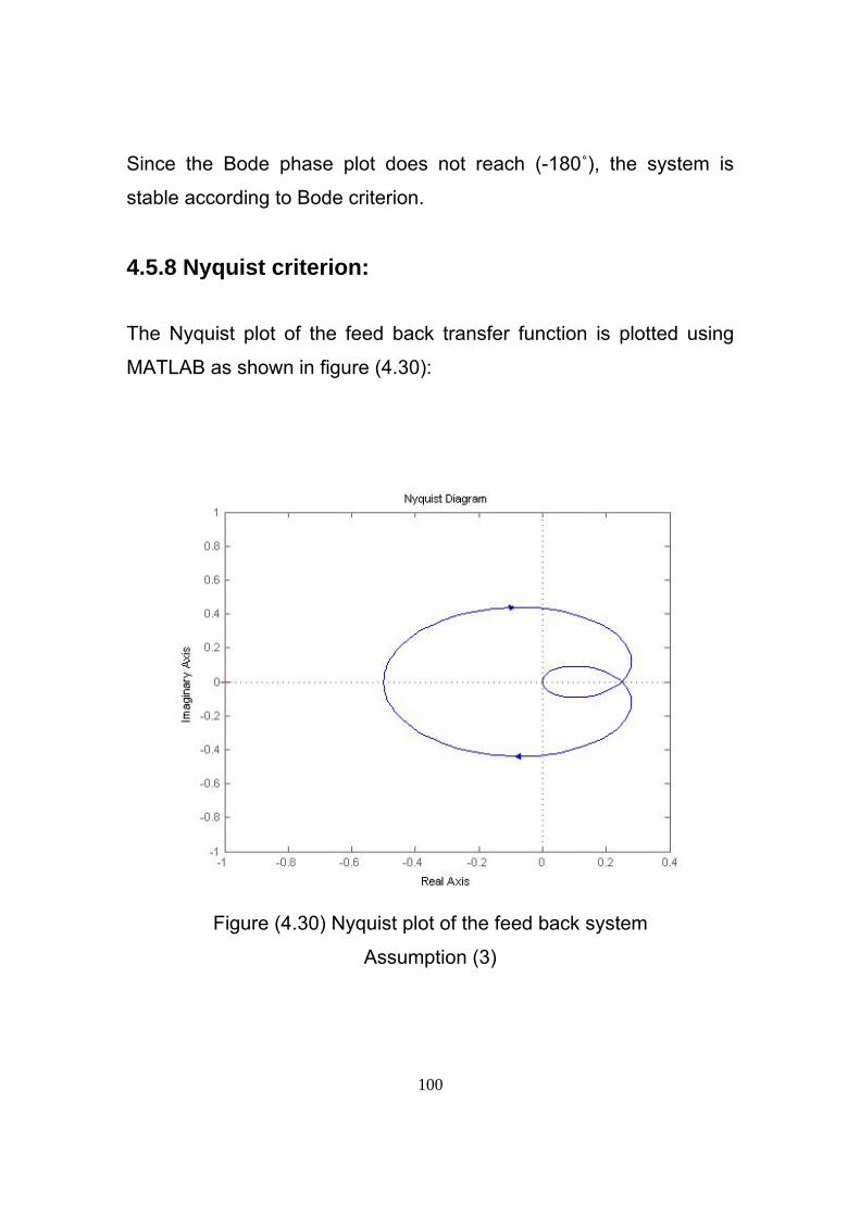
100
Since the Bode phase plot does not reach (-180˚), the system is
stable according to Bode criterion.
4.5.8 Nyquist criterion:
The Nyquist plot of the feed back transfer function is plotted using
MATLAB as shown in figure (4.30):
Figure (4.30) Nyquist plot of the feed back system
Assumption (3)
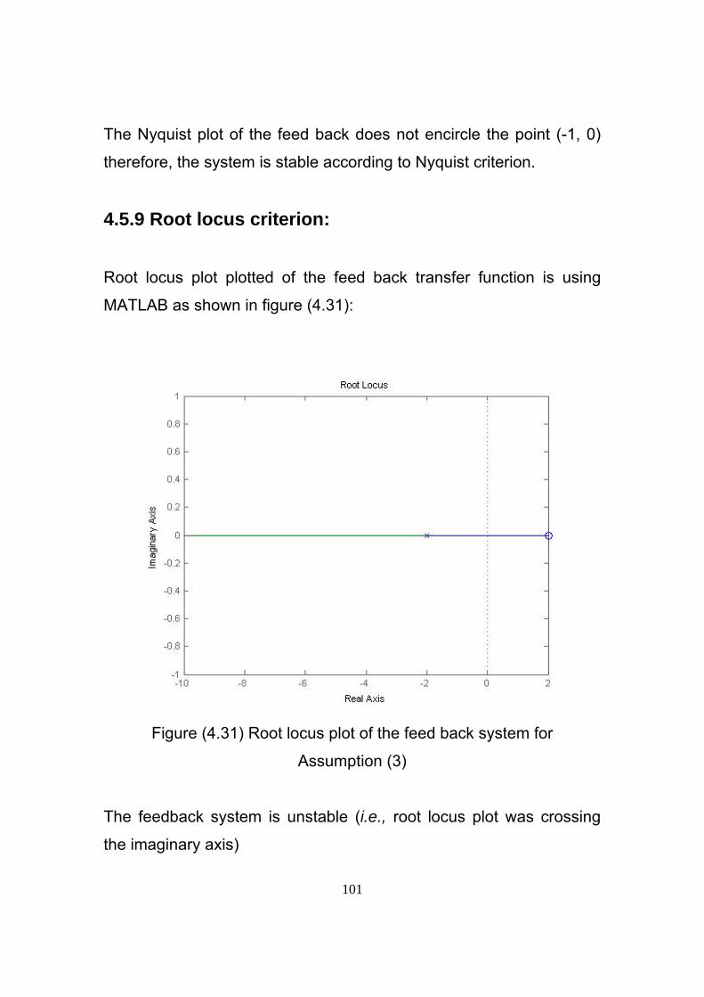
101
The Nyquist plot of the feed back does not encircle the point (-1, 0)
therefore, the system is stable according to Nyquist criterion.
4.5.9 Root locus criterion:
Root locus plot plotted of the feed back transfer function is using
MATLAB as shown in figure (4.31):
Figure (4.31) Root locus plot of the feed back system for
Assumption (3)
The feedback system is unstable (i.e., root locus plot was crossing
the imaginary axis)
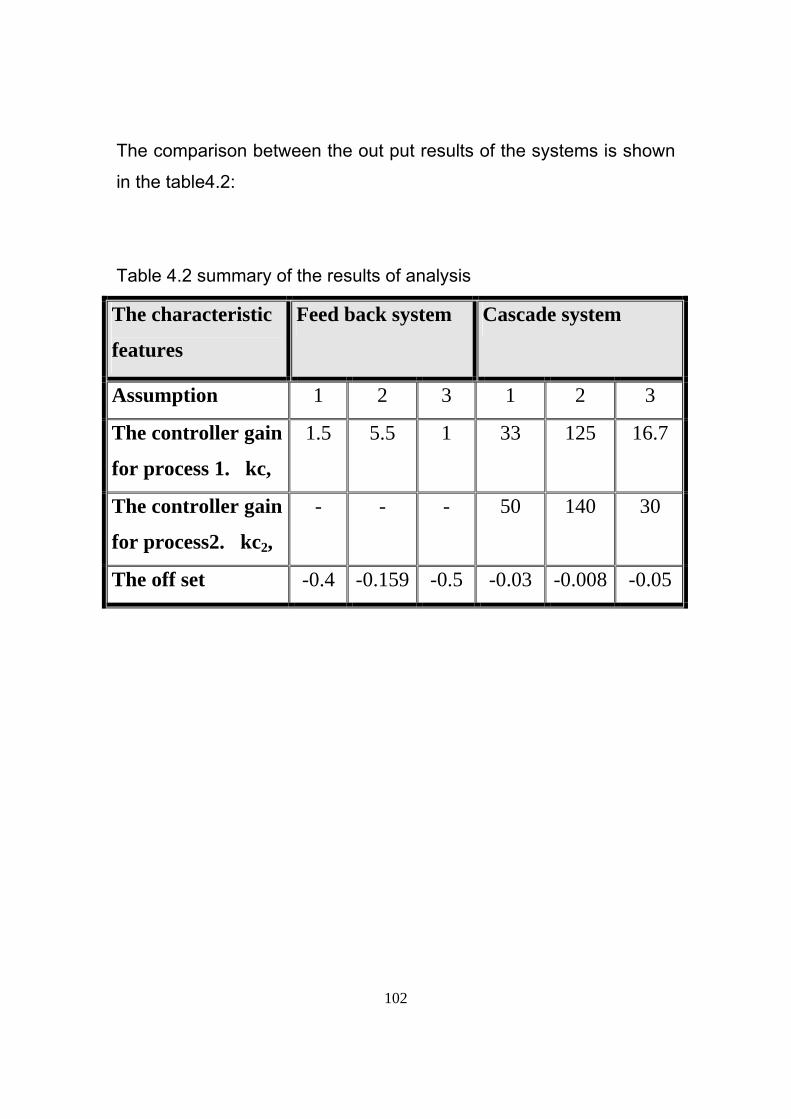
102
The comparison between the out put results of the systems is shown
in the table4.2:
Table 4.2 summary of the results of analysis
Cascade system Feed back system The characteristic
features
3 2 1 3 2 1 Assumption
16.7 125 33 1 5.5 1.5 The controller gain
for process 1. kc,
30 140 50 - - - The controller gain
for process2. kc2,
-0.05 -0.008-0.03 -0.5 -0.159-0.4 The off set
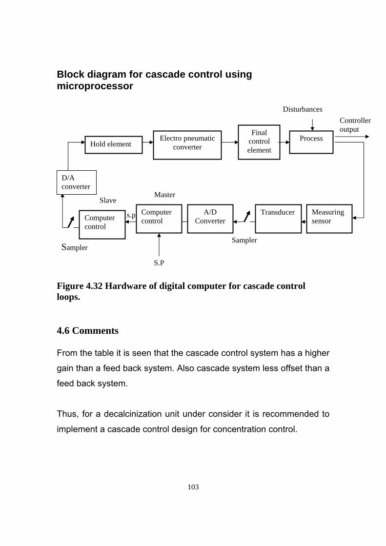
103
Block diagram for cascade control using microprocessor s.p Figure 4.32 Hardware of digital computer for cascade control loops.
4.6 Comments From the table it is seen that the cascade control system has a higher
gain than a feed back system. Also cascade system less offset than a
feed back system.
Thus, for a decalcinization unit under consider it is recommended to
implement a cascade control design for concentration control.
Electro pneumatic converter Hold element
Process Final
control element
Computer control
Computer control
A/D Converter
Transducer Measuring sensor
D/A converter
Sampler
Slave Master
Sampler
S.P
Disturbances Controller output

104
Chapter Five
Conclusions and
Recommendations
105
Conclusion and Recommendation
5.1 Conclusions
In chapter one, of this thesis various processes of crude oil treatment in oil
refinery were discussed including the process of desalting. It was also high
lighted how salts in treated crude might affect on its quality and refinery
units. Moreover, the importance of control systems, crude oil in refineries
was discussed. Finally, research objectives were stated.
In chapter two description for process of crude oil desalting, desalting
methods and decalcinization were explained. Also, control system was
defined; supported with a brief historical background. Meanwhile, control
system’s design, types, tuning loops and stability criteria were investigated
thoroughly.
In chapter three, cascade control instruments, feedback control instruments.
Followed by types of controllers suggested for the case study and types of
sensors. Also, mathematical models were formulated for the case study
desalting unit. Feed back and Cascade control systems for decalcinization
injection in a desalting unit were studied through considering different
assumptions. These two control systems for decalcinization addition in a
desalting unit were suggested for comparative studies.
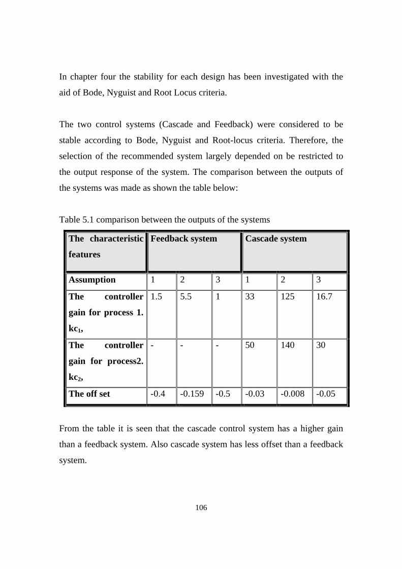
106
In chapter four the stability for each design has been investigated with the
aid of Bode, Nyguist and Root Locus criteria.
The two control systems (Cascade and Feedback) were considered to be
stable according to Bode, Nyguist and Root-locus criteria. Therefore, the
selection of the recommended system largely depended on be restricted to
the output response of the system. The comparison between the outputs of
the systems was made as shown the table below:
Table 5.1 comparison between the outputs of the systems
Cascade system Feedback system The characteristic
features
3 2 1 3 2 1 Assumption
16.7 125 33 1 5.5 1.5 The controller
gain for process 1.
kc1,
30 140 50 - - - The controller
gain for process2.
kc2,
-0.05 -0.008 -0.03 -0.5 -0.159 -0.4 The off set
From the table it is seen that the cascade control system has a higher gain
than a feedback system. Also cascade system has less offset than a feedback
system.

107
Thus, for a decalcinization addition in a desalting unit under considers it is
recommended that a cascade control design is implemented.
108
5.2 Recommendation
Only two types of control systems configurations were considered in this
research, feedback and cascade. It is recommended therefore that addition
control structures are considered in order to draw amore comprehensive
conclusion.
Controller dead time and time constant were not measured nor calculated
in this research. Reasonable values for these properties were assumed. It
time and resources allow, it is recommended that these values are
measured in order to reflect a more accurate results
Since it was assumed in this research that obtaining reliable outputs in
short time will cover the cost of the suggested cascade control system
purchase and installation, more detailed economical studies are
recommended in order to take this into consideration.
109
References
(1) George Stephanopoulos, 2004, Chemical Process Control, Massachusetts Institute of Technology. (2) Abu Goukh M. E, 2003, Controlling Techniques and system Stability, U of K. (3) Abu Goukh M. E, 2002, Process Dynamic and Control, U of K. (4) Oil and Gas Magazine “Issue NO 18th_ July 2008” (5) www.google.com/ crude oil desalting, 2008 NACTO (6) www.google.com/ patent & report, Patent No 6905593, 2005 (7) Report H. Perry, 1997, PERRY’S CHEMICAL ENGINEER’S HANDBOOK, Library of Congress Cataloging-in- Publication Data (8) P_Harriot, 1984, Process Control, McGraw Hill.