Embed Size (px)
Citation preview

Control of industrial robots
Robot dynamics
Prof. Paolo Rocco ([email protected])Politecnico di MilanoDipartimento di Elettronica, Informazione e Bioingegneria

Control of industrial robots – Robot dynamics – Paolo Rocco
Introduction
With these slides we will derive the dynamic model of the manipulator
The dynamic model accounts for the relation between the sources of motion (forces and moments) and the resulting motion (positions and velocities)
u(t)
q(t)
Systematic methods exist to derive the dynamic model of the manipulators, which will be reviewed here, along with the main properties of such model
Control of industrial robots – Robot dynamics – Paolo Rocco
Kinetic energy
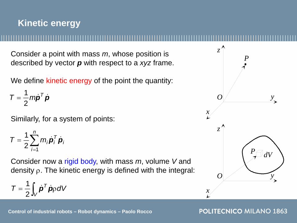
Consider a point with mass m, whose position is described by vector p with respect to a xyz frame.
We define kinetic energy of the point the quantity:
P
x
y
z
Opp TmT21
=
Consider now a rigid body, with mass m, volume V and density ρ. The kinetic energy is defined with the integral:
∫ ρ=V
T dVT pp 21
P
x
y
z
O
dV
Similarly, for a system of points:
∑=
=n
ii
TiimT
121 pp

Control of industrial robots – Robot dynamics – Paolo Rocco
Potential energy
A system of position forces (i.e. depending only on the positions of the points of application) is said to be conservative is the work made by each force does not depend on the trajectory followed by the point of application, but only on the initial and final positions.In this case the elementary work coincides with the differential, with changed sign, of a function called potential energy:
dUdW −=
An example of a system of conservative forces is the gravitational force.For a point mass we have the potential energy:
pgTmU 0−=
For a rigid body:
lT
V
T mdVU pgpg 00 −=ρ−= ∫
where g0 is the gravity acceleration vector.
where pl is the position of the center of mass.

Control of industrial robots – Robot dynamics – Paolo Rocco
Systems of rigid bodies
Let us consider a system of r rigid bodies (as for example, the links of a robot). If all these bodies are free to move in space, the motion of the system is, at each time instant, described by means of 6r coordinates x.
Suppose now that limitations exist in the motion of the bodies of the system (as for example the presence of a joint, which eliminates five out of the six relative degrees of freedom between two consecutive links).A constraint thus exists on the motion of the bodies, which we will express with the relation:
( ) 0=xh
Such a constraint is said to be holonomic (it depends only on position coordinates, not velocities) and stationary (it does not change with time).

Control of industrial robots – Robot dynamics – Paolo Rocco
Free coordinates
( ) 0=xh
If the constraints h are composed of s scalar equations and they are all continuously differentiable, it is possible, by means of the constraints, to eliminate s coordinates from the system equations.
The remaining n = 6r – s coordinates are called free, or Lagrangian, or natural, or generalized coordinates. n is the number of degrees of freedom of the mechanical system.
For example in a robot with 6 joints, out of the 36 original coordinates, 30 are eliminated by virtue of the constraints imposed by the 6 joints. The remaining 6 are the Lagrangian coordinates (typically the joint variables used in the kinematic model).

Control of industrial robots – Robot dynamics – Paolo Rocco
Lagrange’s equations
( ) ( ) ( )qqqqq UTL −= ,,
∑=
ξ=n
iiidqdW
1
Given a system of rigid bodies, whose positions and orientations can be expressed by means of n generalized coordinates qi, we define Lagrangian of the mechanical system the quantity:
where T and U are the kinetic and the potential energies, respectively. Let then ξi be the generalized forces associated with the generalized coordinates qi. The elementary work performed by the forces acting on the system can be expressed as:
It can be proven that the dynamics of the system of bodies is expressed by the following Lagrange’s equations:
niqL
qL
dtd
iii
,,1,
=ξ=∂∂
−∂∂

Control of industrial robots – Robot dynamics – Paolo Rocco
An example
Let us consider a system composed of a motor rigidly connected to a load, subjected to the gravitational force. Let: Im and Ii the moments of inertia of the
motor and the load with respect to the motor spinning axis
m the mass of the load l the distance of the center of mass of the
load from the axis of the motor.
Kinetic energy of the motor: 2
21
ϑ= mm IT
mg
ϑ
τ
l x
y
C
Kinetic energy of the load: 2
21ϑ= ITc

Control of industrial robots – Robot dynamics – Paolo Rocco
Gravitational potential energy:
Lagrangian: ( ) ϑ−ϑ+=−+= sin21 2 lmgIIUTTL mcm
Lagrange’s equations:
mg
ϑ
τ
l [ ] ϑ=
ϑϑ
−−=−= sinsincos
00 lll
mggmmU lT pg
( )( ) τ=ϑ+ϑ+⇒τ=ϑ∂∂
−ϑ∂∂ coslmgII
dtdLL
dtd
m
Then:
( ) τ=ϑ+ϑ+ coslmgII m This equation can be easily interpreted as the
equilibrium of moments around the rotation axis.
An example

Control of industrial robots – Robot dynamics – Paolo Rocco
Kinetic energy of a link
The contribution of kinetic energy of a single link can be computed with the following integral:
∫ ρ=iV
iT
ii dVT **
21 pp
generic point along the link*ip
Position of the center of mass: ∫ ρ=i
i Vi
il dV
m*1 pp
Velocity of the generic point: ( ) iiliili iirSprpp ωω +=×+= *
where: ( )
ωω−ω−ωωω−
=0
00
ixiy
ixiz
iyiz
iωS (skew-symmetric matrix)

Control of industrial robots – Robot dynamics – Paolo Rocco
Translational contribution:
iii
ii lT
liV
lT
l mdV pppp 21
21
=ρ∫Mutual contribution:
( ) ( ) ( ) 0* =ρ−=ρ ∫∫i
iii
i Vlii
Tl
Vii
Tl dVdV ppSprSp ωω
Rotational contribution:
( ) ( ) ( ) ( ) iiTii
Vii
TTi
Viii
TTi
ii
dVdV ωωωωωω IrSrSrSSr21
21
21
=
ρ=ρ ∫∫ ( ) ( ) iiii ωω rSrS −=
Note:
Kinetic energy of a link
Then: iiTil
Tlii ii
mT ωω Ipp21
21
+=
velocity of center of mass
angular velocity of the link
König Theorem
Control of industrial robots – Robot dynamics – Paolo Rocco
Inertia tensor
iTi
ii ωω R=
(symmetric matrix)
( )( )
( )
−−−
=
ρ+
ρ−ρ+
ρ−ρ−ρ+
=
∫∫∫∫∫∫
izz
iyziyy
ixzixyixx
iyix
iziyizix
izixiyixiziy
i
IIIIII
dVrr
dVrrdVrr
dVrrdVrrdVrr
***
**
*22
22
22
I
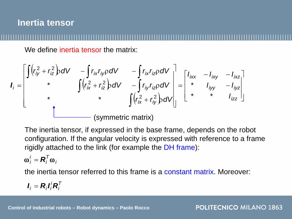
The inertia tensor, if expressed in the base frame, depends on the robot configuration. If the angular velocity is expressed with reference to a frame rigidly attached to the link (for example the DH frame):
the inertia tensor referred to this frame is a constant matrix. Moreover:Ti
iiii RIRI =
We define inertia tensor the matrix:

Control of industrial robots – Robot dynamics – Paolo Rocco
Sum of the contributions
Let us sum the translational and rotational contributions:
iTi
iii
Til
Tlii ii
mT ωω RIRpp21
21
+=
Linear velocity:
( ) ( ) ( )qJjjp iiii
lPi
lPi
lPl qq =++= 11
( ) ( ) ( )[ ]00 iii lPi
lP
lP jjJ 1=
Angular velocity:
( ) ( ) ( )qJjj iii lOi
lOi
lOi qq =++= 11ω ( ) ( ) ( )[ ]00 iii l
Oil
Ol
O jjJ 1=
Control of industrial robots – Robot dynamics – Paolo Rocco
Computation of the Jacobians
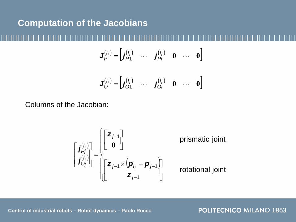
( ) ( ) ( )[ ]00 iii lPi
lP
lP jjJ 1=
( ) ( ) ( )[ ]00 iii lOi
lO
lO jjJ 1=
( )
( ) ( )
−×
=
−
−−
−
joint rotational
jointprismatic
1
11
1
j
jlj
j
lOj
lPj
i
i
i
zppz
z
jj 0
Columns of the Jacobian:
Control of industrial robots – Robot dynamics – Paolo Rocco
Inertia matrix
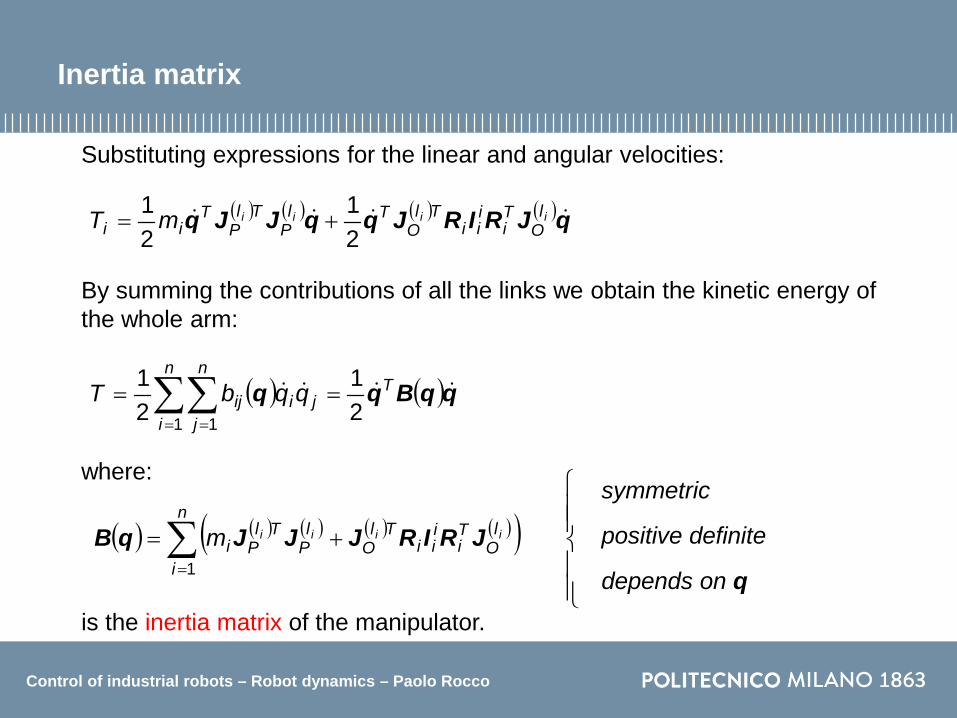
Substituting expressions for the linear and angular velocities:
( ) ( ) ( ) ( )qJRIRJqqJJq iiii lO
Ti
iii
TlO
TlP
TlP
Tii mT
21
21
+=
By summing the contributions of all the links we obtain the kinetic energy of the whole arm:
( ) ( )qqBqq Tn
i
n
jjiij qqbT
21
21
1 1
== ∑∑= =
where:
( ) ( ) ( ) ( ) ( )( )∑=
+=n
i
lO
Ti
iii
TlO
lP
TlPi
iiiim1
JRIRJJJqB
is the inertia matrix of the manipulator.
symmetric
positive definite
depends on q

Control of industrial robots – Robot dynamics – Paolo Rocco
Potential energy
The potential energy of a rigid link is related just to the gravitational force:
ilT
iV
iT
i mdVU pgpg 0*
0 −=ρ−= ∫where g0 is the gravity acceleration vector expressed in the base frame.
The potential energy of the whole manipulator is then the sum of the single contributions:
∑∑==
−==n
il
Ti
n
ii i
mUU1
01
pg

Control of industrial robots – Robot dynamics – Paolo Rocco
Equations of motion
The Lagrangian of the manipulator is:
( ) ( ) ( ) ( ) ( )∑∑∑== =
+=−=n
ili
Ti
n
i
n
jjiij mqqbUTL
10
1 121,, qpgqqqqqq
If we differentiate the Lagrangian:
Furthermore:
( )( ) ( )qqjgp
g i
n
j
lP
Tj
n
j i
ljTj
igm
qm
qU j
i=−=
∂
∂−=
∂∂ ∑∑
== 10
10
( ) ( ) ( )
( ) ( )∑ ∑∑
∑∑∑
= ==
===
∂
∂+=
=+=
=
∂∂
=
∂∂
n
jj
n
kk
k
ijn
jjij
n
jj
ijn
jjij
n
jjij
ii
qqq
bqb
qdt
dbqbqb
dtd
qT
dtd
qL
dtd
1 11
111
qqq
( )∑∑= = ∂
∂=
∂∂ n
j
n
kjk
i
jk
iqq
qb
qT
1 121
q
Control of industrial robots – Robot dynamics – Paolo Rocco
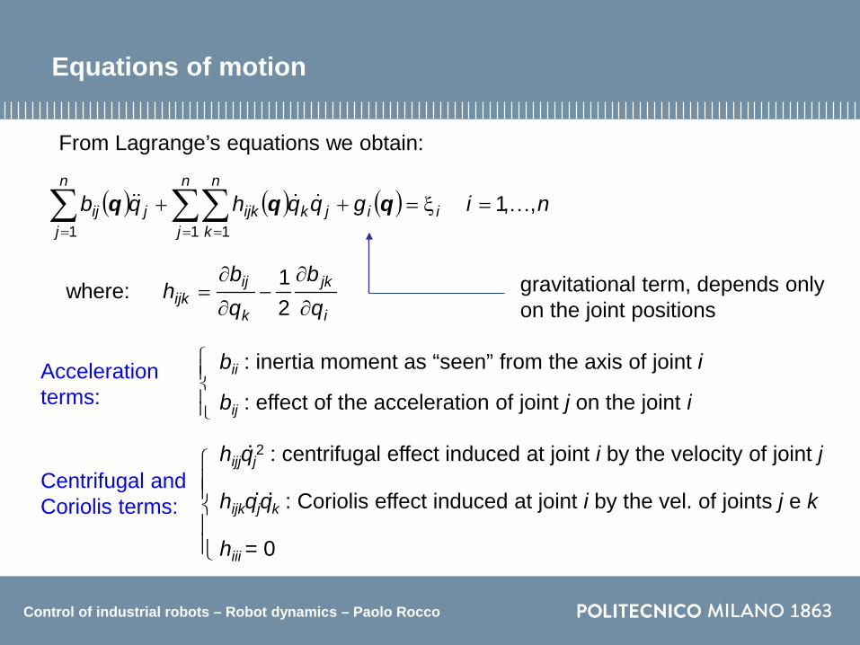
From Lagrange’s equations we obtain:
where:
( ) ( ) ( ) nigqqhqb ii
n
j
n
kjkijk
n
jjij ,,1
1 11
=ξ=++∑∑∑= ==
qqq
i
jk
k
ijijk q
bqb
h∂
∂−
∂
∂=
21
Acceleration terms:
bii : inertia moment as “seen” from the axis of joint i
bij : effect of the acceleration of joint j on the joint i
Centrifugal and Coriolis terms:
hijjqj2 : centrifugal effect induced at joint i by the velocity of joint j
hijkqjqk : Coriolis effect induced at joint i by the vel. of joints j e k
.
. .
gravitational term, depends only on the joint positions
hiii = 0
Equations of motion

Control of industrial robots – Robot dynamics – Paolo Rocco
Non conservative forces
Besides the gravitational conservative forces, other forces act on the manipulator:
actuation torques
viscous friction torques
static friction torques
τ
qF v−
( )qqf ,s−
diagonal matrix of viscous friction coefficientsvF
( )qqf ,s function that models the static friction at the joint

Control of industrial robots – Robot dynamics – Paolo Rocco
Complete dynamic model
In vector form the dynamic model can be expressed as follows:
( ) ( ) ( ) ( ) τ=++++ qgqqfqFqqqCqqB ,, sv
where C is a suitable n×n matrix, whose elements satisfy the equation:
∑∑∑= ==
=n
j
n
kjkijk
n
jjij qqhqc
1 11
C is not symmetric in general

Control of industrial robots – Robot dynamics – Paolo Rocco
Computation of the elements of C
The choice of matrix C is not unique. One possible choice is the following one:
∑∑∑∑
∑∑∑∑∑
= == =
= == ==
∂
∂−
∂∂
+∂
∂=
=
∂
∂−
∂
∂==
n
j
n
kjk
i
jk
j
ikn
j
n
kjk
k
ij
n
j
n
kjk
i
jk
k
ijn
j
n
kjkijk
n
jjij
qqqb
qbqq
qb
qqqb
qb
qqhqc
1 11 1
1 11 11
21
21
21
The generic element of C is:
∑=
=n
kkijkij qcc
1
∂
∂−
∂∂
+∂
∂=
i
jk
j
ik
k
ijijk q
bqb
qb
c21 Christoffel symbols of the
first kindwhere:

Control of industrial robots – Robot dynamics – Paolo Rocco
Skew-symmetry of matrix B−2C
The previous choice of matrix C allows to prove an important property of the dynamic model of the manipulator. Matrix:
∑∑∑===
∂
∂−
∂∂
+=
∂
∂−
∂∂
+∂
∂=
n
kk
i
jk
j
ikij
n
kk
i
jk
j
ikn
kk
k
ijij q
qb
qbbq
qb
qbq
qb
c111 2
121
21
21
.
( ) ( ) ( )qqCqBqqN ,2, −=
is skew-symmetric:
( ) wwqqNw ∀= ,0, T
In fact:
∑=
∂∂
−∂
∂=−=
n
kk
j
ik
i
jkijijij q
qb
qb
cbn1
2 jiij nn −= (skew-symmetric)

Control of industrial robots – Robot dynamics – Paolo Rocco
Energy conservation
The equation:
( ) 0, =qqqNq T
(particular case of the previous one) is valid whatever the choice of matrix C is. From the energy conservation principle, the derivative of the kinetic energy equals the power generated by all the forces acting at the joint of the manipulator:
( )( ) ( ) ( )( )qgqqfqFqqqBq −−−= ,21
svTT
dtd
τ
Taking the derivative at the left hand side and using the equation of the model:
( )( ) ( ) ( ) ( ) ( )( )
( ) ( )( )qgqqfqFq
qqqCqBqqqBqqqBqqqBq
−−−+
−=+=
,
,221
21
21
svT
TTTT
dtd
τ from which the equation follows.
Control of industrial robots – Robot dynamics – Paolo Rocco
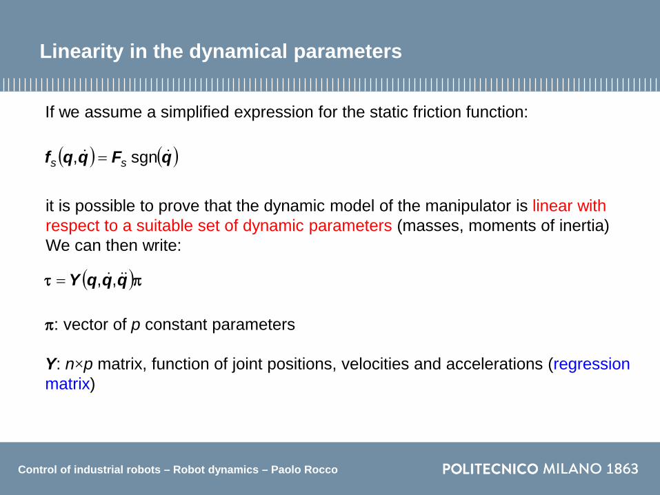
Linearity in the dynamical parameters
If we assume a simplified expression for the static friction function:
( ) ( )qFqqf sgn, ss =
π: vector of p constant parameters
Y: n×p matrix, function of joint positions, velocities and accelerations (regression matrix)
( )πτ qqqY ,,=
it is possible to prove that the dynamic model of the manipulator is linear with respect to a suitable set of dynamic parameters (masses, moments of inertia)We can then write:

Control of industrial robots – Robot dynamics – Paolo Rocco
Two-link Cartesian manipulator
Consider a two-link Cartesian manipulator, characterized by link masses m1 e m2.The vector of generalized coordinates is:
The Jacobians needed for the computation of the inertia matrix are:
=
2
1
dd
q
( ) ( )[ ] [ ]
( ) ( ) ( )[ ] [ ]
===
===
010010
010000
10
0
2
2
2
1
2
1
1
1
zzjjJ
zjJ
lP
lP
lP
lP
lP 00
while there are no contributions to the angular velocities.
x0
z0
z1
m1
m2
d1
d2

Control of industrial robots – Robot dynamics – Paolo Rocco
Computing the inertia matrix with the general formula, we obtain:
As B is constant, C=0, i.e. there are no centrifugal and Coriolis terms.Then, since:
the vector of the gravitational terms is:
−=
g00
0g
( ) ( ) ( ) ( )
+=+=
2
2121 0
02211
mmm
mm lP
TlP
lP
TlP JJJJB
( )
+=
021 gmm
g
Two-link Cartesian manipulator

Control of industrial robots – Robot dynamics – Paolo Rocco
If there are no friction torques and no forces at the end-effector:
( ) ( )222
121121
fdm
fgmmdmm
=
=+++
f1 e f2: forces which act along the generalized coordinates
Two-link Cartesian manipulator

Control of industrial robots – Robot dynamics – Paolo Rocco
Two-link planar manipulator
Let us consider a two-link planar manipulator: masses: m1 and m2 lengths: a1 and a2 distances of the centers of mass from the joint axes: l1
and l2 moments of inertia around axes passing through the
centers of mass and parallel to z0: I1 and I2
ϑϑ
=2
1q
m1, I1
m2, I2
a1
a2
ϑ1
ϑ2
l1
l2
x0
y0
The Jacobians needed for the computation of the inertia matrix depend on the following vectors:
=
=
++
=
=
0,
000
,0
,0
11
11
1012211
12211
11
11
21saca
ssacca
sc
ll pppp ll
ll
Generalized coordinates:
==
100
10 zz
Control of industrial robots – Robot dynamics – Paolo Rocco
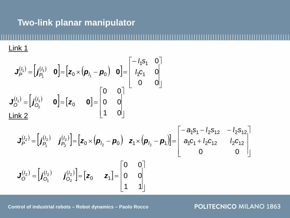
Two-link planar manipulator
Link 1
( ) ( )[ ] ( )[ ]
−=−×==
0000
11
11
00 111
1 cs
ll
Pl
P ll
00 ppzjJ
( ) ( )[ ] [ ]
===
010000
01
1
1 00 zjJ lO
lO
Link 2
( ) ( ) ( )[ ] ( ) ( )[ ]
+
−−−=−×−×==
0012212211
12212211
1100 2222
21
2 cccasssa
lll
Pl
Pl
P llll
ppzppzjjJ
( ) ( ) ( )[ ] [ ]
===
110000
102
2
2
1
2 zzjjJ lO
lO
lO

Control of industrial robots – Robot dynamics – Paolo Rocco
Taking into account that the angular velocity vectors ω1 and ω2 are aligned with z0it is not necessary to compute rotation matrices Ri , so that the computation of the inertia matrix gives:
( ) ( ) ( ) ( ) ( ) ( ) ( ) ( ) ( ) ( ) ( )( )
( )( )
222222
22212222112
222122
2121
21111
2221
12112121
2
22112211
Imb
Icambb
IcaamImb
bbbb
IImm lO
TlO
lO
TlO
lP
TlP
lP
TlP
+=
++==
+++++=
ϑ
ϑϑ=+++=
l
ll
lll
JJJJJJJJqB
Two-link planar manipulator
depends on ϑ2
depends on ϑ2
constant!

Control of industrial robots – Robot dynamics – Paolo Rocco
From the inertia matrix it is simple to compute the Christoffel symbols:
021
0212121
21
021
2
22222
1
22221212
22122
11
1
21211
22121
22
2
12122
22122
11121112
1
11111
=∂∂
=
=∂∂
==
−==∂∂
−∂∂
=
=−=∂∂
−∂∂
=
=−=∂∂
==
=∂∂
=
qbc
qbcc
hsamqb
qbc
hsamqb
qbc
hsamqbcc
qbc
l
l
l 2212 samh l−=
Two-link planar manipulator

Control of industrial robots – Robot dynamics – Paolo Rocco
The expression of matrix C is then:
( ) ( ) ( )
ϑϑ+ϑ−ϑ−
=
ϑ−ϑ+ϑϑ
=00
,12212
21221222212
1
212
samsamsam
hhh
lllqqC
We can verify that matrix N is skew-symmetric:
( ) ( ) ( ) ( )
( )qqN
qqCqBqqN
,02
20
02
02,2,
21
21
1
212
2
22
T
hhhh
hhh
hhh
−=
ϑ+ϑϑ−ϑ−
=
=
ϑ−ϑ+ϑϑ
−
ϑϑϑ
=−=
Furthermore, since g0 = [0 −g 0]T, the vector of the gravitational terms is:
( )
++=
1222
122211211
cgmcgmgcamm
lll
g
Two-link planar manipulator

Control of industrial robots – Robot dynamics – Paolo Rocco
τi : torques applied at the joints
( )( ) ( )( )
( ) 1122211211
222212212212
2222122212221
22
2121
211
2
2
τ=+++
+ϑ−ϑϑ−
+ϑ+++ϑ+++++
cgmgcammsamsam
IcamIcaamIm
llll
lllll
( )( ) ( )21222
212212
2222212221
222
τ=+ϑ+
+ϑ++ϑ++
gcmsam
ImIcam
ll
lll
Without friction at the joints, the equations of motion are:
Two-link planar manipulator

Control of industrial robots – Robot dynamics – Paolo Rocco
By simple inspection, we can obtain the dynamical parameters with respect to which the model is linear, i.e. those parameters for which we can write:
( )πτ qqqY ,,=
We have:
[ ]T54321 πππππ=π
22225
224
23
21112
111
l
l
l
l
mI
mm
mI
m
+=π
=π
=π
+=π
=π
Two-link planar manipulator

Control of industrial robots – Robot dynamics – Paolo Rocco
2125
12212112124
2115
122221212122112114
1112113
112
111
22
ϑ+ϑ=
+ϑ+ϑ=
ϑ+ϑ=
+ϑ−ϑϑ−ϑ+ϑ=
+ϑ=
ϑ=
=
y
gcsacay
y
gcsasacacay
gcaay
y
gcy
( )
=
2524
1514131211
000,,
yyyyyyy
qqqY
The coefficients of Y depend on ϑ1, ϑ2, their first and second derivatives, g and a1.
Two-link planar manipulator

Control of industrial robots – Robot dynamics – Paolo Rocco
Identification of dynamical parameters
The linearity of the dynamic model with respect to the dynamical parameters:
( )πτ qqqY ,,=
allows to setup a procedure for the experimental identification of the same parameters, which are usually unknown or uncertain.
Suitable motion trajectories must be executed, along which the joint positions q are recorded, the velocities q are measured or obtained by numerical differentiation, and the accelerations q are obtained with filtered (also non-causal) differentiation.Also the torques τ are measured, directly (with suitable sensors) or indirectly, from the measurements of currents in the motors.
Suppose to have the measurements (direct or indirect ones) of all the variables for the time instants t1, …, tN.
...
Control of industrial robots – Robot dynamics – Paolo Rocco
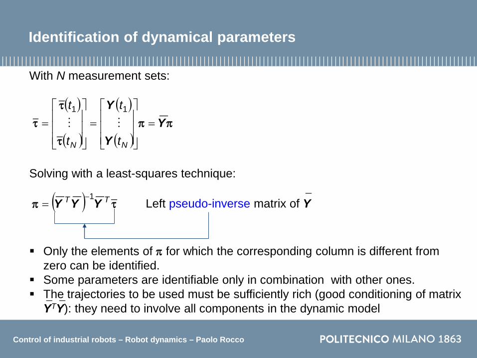
With N measurement sets:
( )
( )
( )
( )ππ
τ
ττ Y
Y
Y=
=
=
NN t
t
t
t
11
Solving with a least-squares technique:
( ) τπ TT YYY1−
= Left pseudo-inverse matrix of Y−
Only the elements of π for which the corresponding column is different from zero can be identified.
Some parameters are identifiable only in combination with other ones. The trajectories to be used must be sufficiently rich (good conditioning of matrix
YTY): they need to involve all components in the dynamic model− −
Identification of dynamical parameters

Control of industrial robots – Robot dynamics – Paolo Rocco
Newton-Euler formulation
An alternative way to formulate the dynamic model of the manipulator is the Newton-Euler method.It is based on balances of forces and moments acting on the single link, due to the interactions with the nearby links in the kinematic chain.
We obtain a system of equations that might be solved in a recursive way, propagating the velocities and accelerations from the base to the end effector, while the forces and moments in the opposite way:
Recursion makes Newton-Euler algorithm computationally efficient.
velo
cities
acce
lerati
ons
forc
esm
omen
ts

Control of industrial robots – Robot dynamics – Paolo Rocco
Definition of the parameters
Let us consider the generic link i of the kinematic chain:
mi and Ii mass and inertia tensor of the linkri-1,Ci vector from the origin of frame (i-1) to the center of mass Ci
ri,Ci vector from the origin of frame i to the center of mass Ci
ri-1, i vector from the origin of frame (i-1) to the origin of frame i
We define the following parameters:
This picture is taken from the textbook:
B. Siciliano, L. Sciavicco, L. Villani, G. Oriolo: Robotics: Modelling, Planning and Control, 3rd Ed. Springer, 2009
Control of industrial robots – Robot dynamics – Paolo Rocco
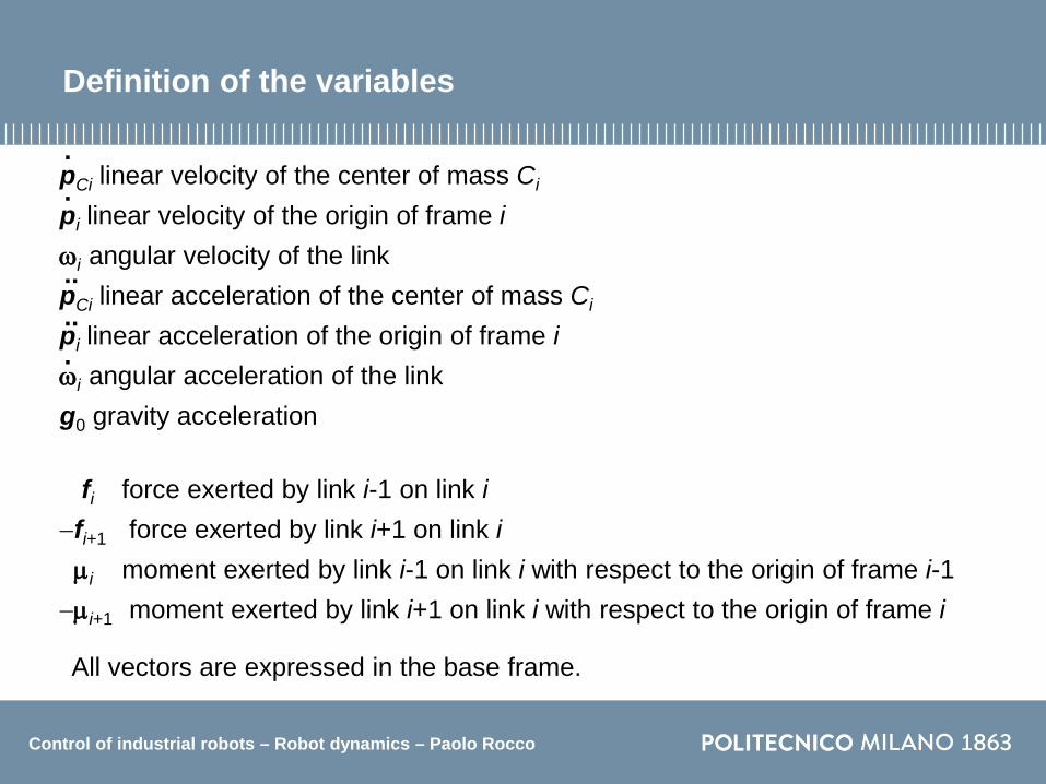
Definition of the variables
pCi linear velocity of the center of mass Ci
pi linear velocity of the origin of frame iωi angular velocity of the linkpCi linear acceleration of the center of mass Ci
pi linear acceleration of the origin of frame iωi angular acceleration of the linkg0 gravity acceleration
.
..
.
.
..
fi force exerted by link i-1 on link i−fi+1 force exerted by link i+1 on link iµi moment exerted by link i-1 on link i with respect to the origin of frame i-1
−µi+1 moment exerted by link i+1 on link i with respect to the origin of frame i
All vectors are expressed in the base frame.

Control of industrial robots – Robot dynamics – Paolo Rocco
Newton-Euler formulation
Newton’s equation (translational motion of the center of mass)
iCiiii mm pgff =+− + 01
Euler’s equation (rotational motion)
( ) ( )iiiiiiiCiiiCiii dtd
iiωωωωµµ IIIrfrf ×+==×−−×+ ++− ,11,1
Generalized force at joint i:
it can be proven gyroscopic effect
=τ−
−
joint rotationaljointprismatic
1
1
iTi
iTi
i zzf
µ

Control of industrial robots – Robot dynamics – Paolo Rocco
Accelerations of a link
Propagation of the velocities:
ϑ+=
−−
−
joint rotationaljointprismatic
11
1
iii
ii zω
ωω
×+×++
=−−
−−−
joint rotationaljointprismatic
,11
,111
iiii
iiiiiii
drp
rzppω
ω
Propagation of the accelerations:
×ϑ+ϑ+=
−−−−
−
joint rotationaljointprismatic
1111
1
iiiiii
ii zz ωω
ωω
( )( )
××+×+××+×+×++
=−−−
−−−−−
joint rotationaljointprismatic 2
,1,11
,1,1111
iiiiiiii
iiiiiiiiiiiiii
ddrrp
rrzzppωωω
ωωωω
( ) mass of center,, iii CiiiCiiiC rrpp ××+×+= ωωω
Note: derivative of a vector ai attached to the moving frame i
( ) ( )
( )( ) ( ) ( ) ( )ttttS
tdtdt
dtd
iiiiii
iiii
aaR
aRa
×==
==
ωω
Control of industrial robots – Robot dynamics – Paolo Rocco
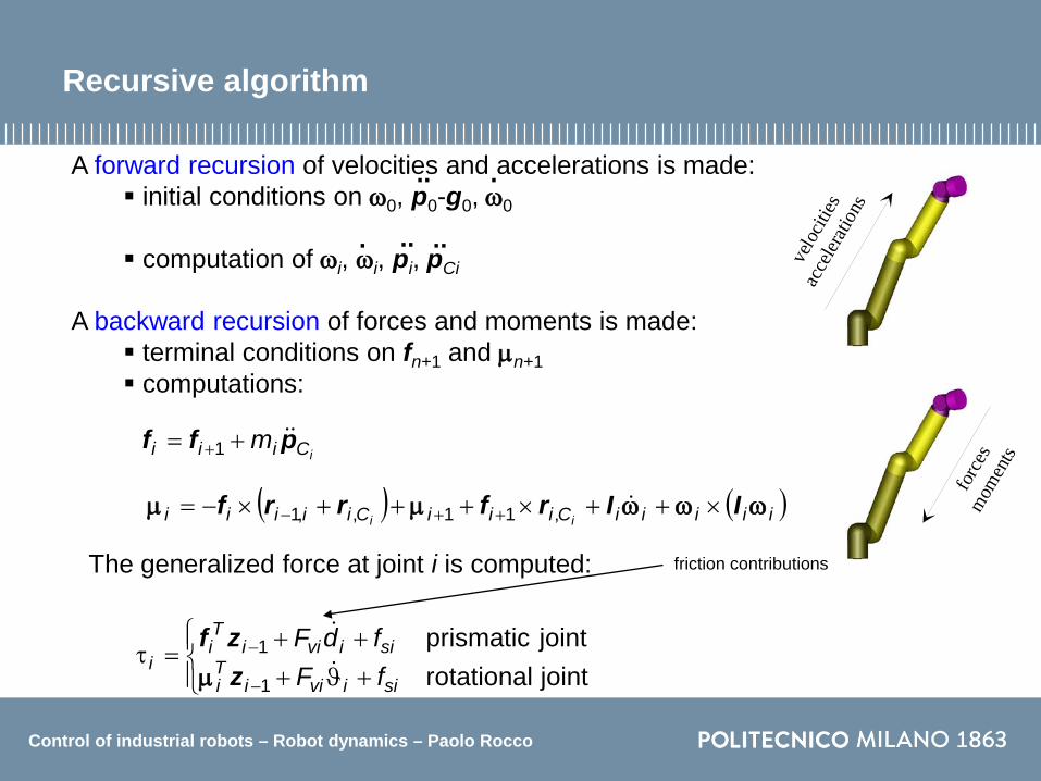
Recursive algorithm
A forward recursion of velocities and accelerations is made: initial conditions on ω0, p0-g0, ω0
computation of ωi, ωi, pi, pCi
.. .
. .. ..
A backward recursion of forces and moments is made: terminal conditions on fn+1 and µn+1 computations:
iCiii m pff += +1
( ) ( )iiiiiCiiiCiiiii iiωωωµµ IIrfrrf ×++×+++×−= ++− ,11,,1
The generalized force at joint i is computed:
+ϑ+++
=τ−
−
joint rotationaljointprismatic
1
1
siiviiTi
siiviiTi
i fFfdF
zzf
µ
friction contributions
velo
cities
acce
lerati
ons
forc
esm
omen
ts

Control of industrial robots – Robot dynamics – Paolo Rocco
Local reference frames
Up to now we have supposed that all the vectors are referred to the base frame.
It is more convenient to express the vectors with respect to the current frame on link i. In this way, vectors ri-1,i e ri,Ci and the inertia tensor Ii are constant, which makes the algorithm computationally more effcient.
The equations are modified in some terms (we need to multiply the vectors by suitable rotation matrices) but nothing changes in the nature of the method.
Control of industrial robots – Robot dynamics – Paolo Rocco
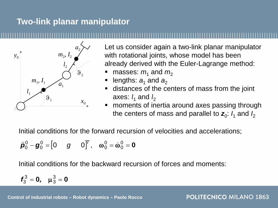
Two-link planar manipulator
Let us consider again a two-link planar manipulator with rotational joints, whose model has been already derived with the Euler-Lagrange method: masses: m1 and m2 lengths: a1 and a2 distances of the centers of mass from the joint
axes: l1 and l2 moments of inertia around axes passing through
the centers of mass and parallel to z0: I1 and I2
Initial conditions for the forward recursion of velocities and accelerations;
[ ] 0===− 00
00
00
00 ,00 ωω Tggp
m1, I1
m2, I2
a1
a2
ϑ1
ϑ2
l1
l2
x0
y0
Initial conditions for the backward recursion of forces and moments:
00 == 33
33 µ,f
Control of industrial robots – Robot dynamics – Paolo Rocco
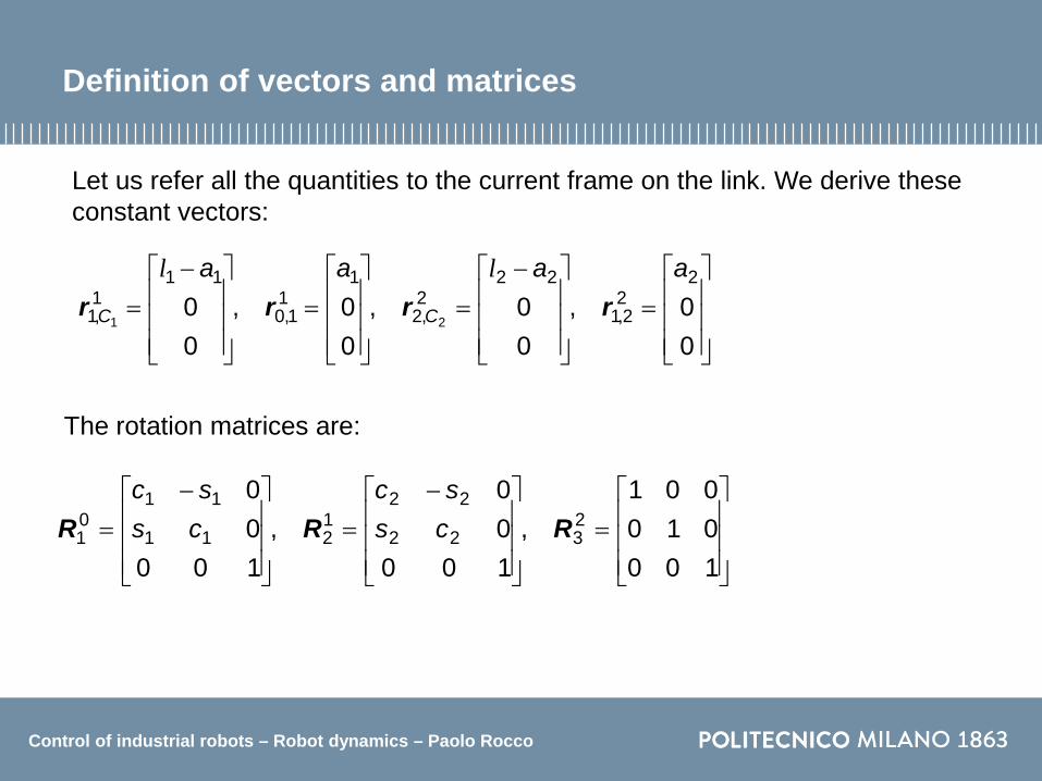
Definition of vectors and matrices
Let us refer all the quantities to the current frame on the link. We derive these constant vectors:
The rotation matrices are:
=
−=
=
−=
00,
00,
00,
00
222,1
222,2
111,0
111,1 21
aaaa
CC rrrrll
=
−=
−=
100010001
,10000
,10000
2322
221211
1101 RRR cs
sccssc

Control of industrial robots – Robot dynamics – Paolo Rocco
Forward recursion: link 1
( )
ϑ=ϑ+=
1
01001
11 0
0
zR ωω T
( )
ϑ=×ϑ+ϑ+=
1
00101001
11 0
0
zzR ωωω T
( )
+ϑ+ϑ−
=××+×+=0
111
1211
11,0
11
11
11,0
110
01
11 gca
gsaT
rrpRp ωωω
( )
+ϑ+ϑ−
=××+×+=0
111
1211
1,1
11
11
1,1
11
11
1111
gcgs
CCC
ll
rrpp ωωω

Control of industrial robots – Robot dynamics – Paolo Rocco
( )
ϑ+ϑ=ϑ+=
21
0211
12
22 0
0
zR ωω T
( )
ϑ+ϑ=×ϑ+ϑ+=
21
011202
11
12
22 0
0
zzR ωωω T
( )( )
( )
+ϑ+ϑ+ϑ+ϑ+ϑ+ϑ−ϑ−ϑ
=××+×+=0
122121212121
122
2122121121
22,1
22
22
22,1
22
11
12
22 gcsaaca
gsacasaT
rrpRp ωωω
( )( )
( )
+ϑ+ϑ+ϑ+ϑ+ϑ+ϑ−ϑ−ϑ
=××+×+=0
122121212121
122
2122121121
2,2
22
22
2,2
22
22
22 22
gcsacagscasa
CCC
ll
rrpp ωωω
Forward recursion: link 2
Control of industrial robots – Robot dynamics – Paolo Rocco
( )( )( )
+ϑ+ϑ+ϑ+ϑ
+ϑ+ϑ−ϑ−ϑ
==+=0
1221212121212
122
21221211212
22
22
33
23
22 22
gcsacam
gscasam
mm CC
l
l
ppfRf
( ) ( )
( )( )
+ϑ+ϑ+ϑ+ϑ+∗∗
=
=×++×+++×−=
12222122121221221
2222
22
22
22
22
22
2,2
33
23
33
23
2,2
22,1
22
22 22
gcmsamcammI
CC
llll
ωωωµµ IIrfRRrrf
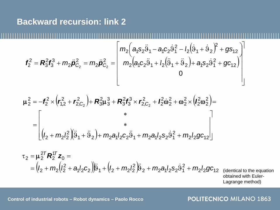
( )( ) ( ) 12222122122
22221221
2222
012
222
gcmsammIcamI
TT
lllll +ϑ+ϑ++ϑ++=
==τ
zRµ
Backward recursion: link 2
(identical to the equation obtained with Euler-Lagrange method)
Control of industrial robots – Robot dynamics – Paolo Rocco
( ) ( ) ( )( ) ( ) ( ) ( )
++ϑ+ϑ−ϑ+ϑ+ϑ+
++ϑ+ϑ−ϑ−ϑ−ϑ+ϑ−
=+=0
1212
212222122211211
1212
212222112
211121222
12
22
12
11 1
gcmmsmcmammgsmmcmammsm
m C
llllll
pfRf
( ) ( )
( ) ( )( )( ) ( )
+++ϑ+ϑ−ϑ+
+ϑ+ϑ+++ϑ+++∗∗
=
=×++×+++×−=
1222112112
212212212212
212222212212212
211
2121
11
11
11
11
11
1,1
22
12
22
12
1,1
11,0
11
11 11
gcmgcammsamsam
mcamIcammamI
CC
llll
llll
ωωωµµ IIrfRRrrf
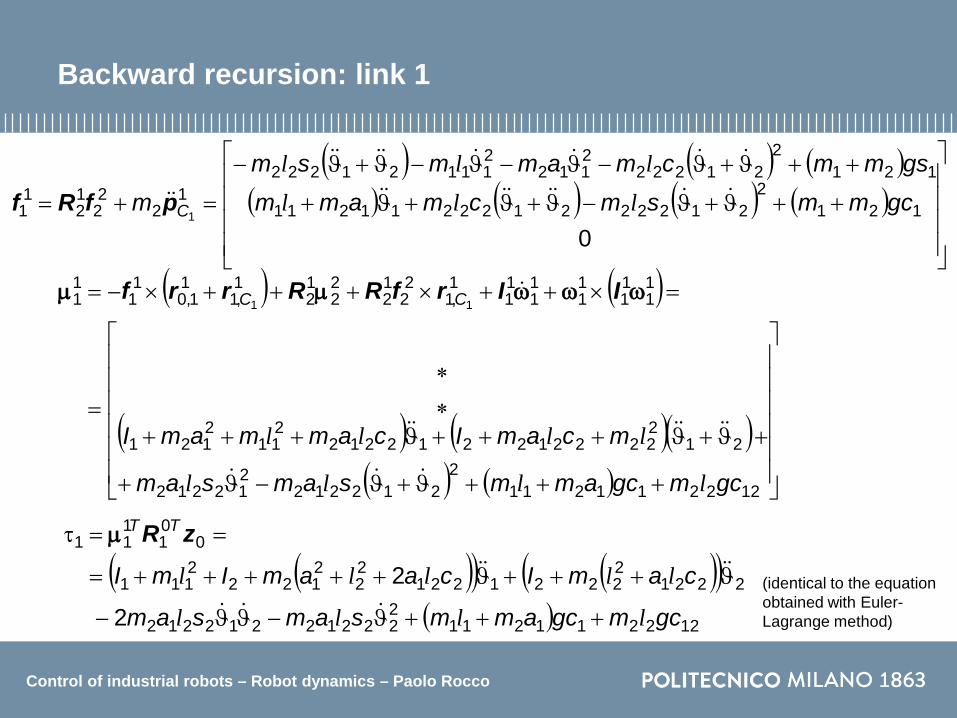
( )( ) ( )( )( ) 122211211
222212212212
222122221221
22
2122
2111
001
111
2
2
gcmgcammsamsam
camIcaamImI
TT
llll
lllll
+++ϑ−ϑϑ−
ϑ+++ϑ+++++=
==τ
zRµ
Backward recursion: link 1
(identical to the equation obtained with Euler-Lagrange method)

Control of industrial robots – Robot dynamics – Paolo Rocco
Euler-Lagrange vs. Newton-Euler
Euler-Lagrange formulation
it is systematic and easy to understand it returns the equations of motion in an analytic and compact form, separating
the inertia matrix, the Coriolis and centrifugal terms, the gravitational terms. All these elements are useful for the design of a model based controller
it lends itself to the introduction into the model of more complex effects (like joint or link deformation)
Newton-Euler formulation
it is a computationally efficient recursive method
Control of industrial robots – Robot dynamics – Paolo Rocco
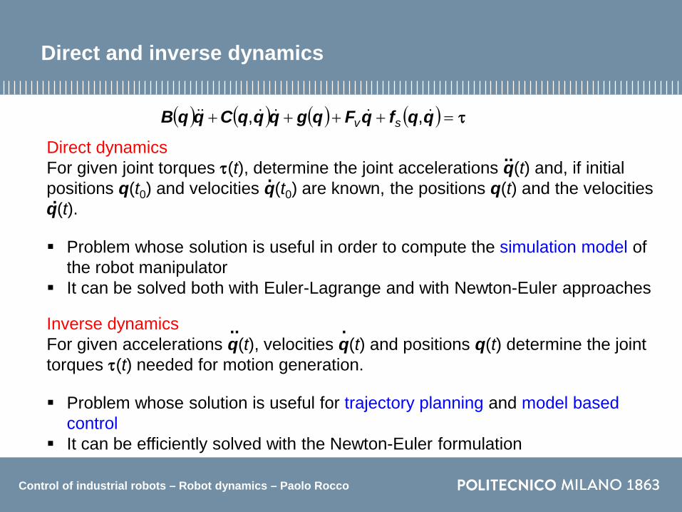
Direct and inverse dynamics
Direct dynamicsFor given joint torques τ(t), determine the joint accelerations q(t) and, if initial positions q(t0) and velocities q(t0) are known, the positions q(t) and the velocities q(t).
( ) ( ) ( ) ( ) τ=++++ qqfqFqgqqqCqqB ,, sv
Inverse dynamicsFor given accelerations q(t), velocities q(t) and positions q(t) determine the joint torques τ(t) needed for motion generation.
...
.
...
Problem whose solution is useful in order to compute the simulation model of the robot manipulator
It can be solved both with Euler-Lagrange and with Newton-Euler approaches
Problem whose solution is useful for trajectory planning and model based control
It can be efficiently solved with the Newton-Euler formulation

Control of industrial robots – Robot dynamics – Paolo Rocco
Computation of direct and inverse dynamics
( ) ( ) τ=+ qqnqqB ,
As for the computation of the direct dynamics, let us rewrite the dynamic model of the manipulator in these terms:
( ) ( ) ( ) ( )qqfqFqgqqqCqqn ,,, sv +++=
where:
Computation of the inverse dynamics can be easily done both with the Euler-Lagrange method and with the Newton-Euler one.
We thus have to numerically integrate the explicit system of differential equations:
( ) ( )( )qqnqBq ,1 −= − τ
where all the elements needed to build the system are directly computed by the Euler-Lagrange method.
Control of industrial robots – Robot dynamics – Paolo Rocco
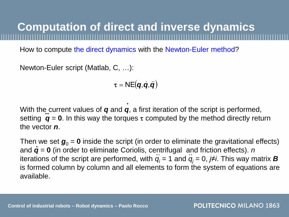
With the current values of q and q, a first iteration of the script is performed, setting q = 0. In this way the torques τ computed by the method directly return the vector n.
How to compute the direct dynamics with the Newton-Euler method?
Then we set g0 = 0 inside the script (in order to eliminate the gravitational effects) and q = 0 (in order to eliminate Coriolis, centrifugal and friction effects). niterations of the script are performed, with qi = 1 and qj = 0, j≠i. This way matrix B is formed column by column and all elements to form the system of equations are available.
.
...
..
..
Computation of direct and inverse dynamics
Newton-Euler script (Matlab, C, …):
( )qqq ,,ΝΕ=τ


![Asimov,Isaac [Robots] (1950) Les robots (I, robot)](https://img.dokumen.tips/doc/110x75/5571f9a34979599169900ec4/asimovisaac-robots-1950-les-robots-i-robot.jpg)