Control and Design of Snake Robots

David Rollinson

TR-14-13

June 2014

School of Computer ScienceCarnegie Mellon University

Pittsburgh, PA 15213

Thesis Committee:Howie Choset, Chair

Chris AtkesonGeorge Kantor

Art Kuo, University of Michigan

Submitted in partial fulfillment of the requirementsfor the degree of Doctor of Philosophy.

Copyright c© 2014 David Rollinson

AbstractSnake robots are ideally suited to highly confined environments because

their small cross-sections and highly redundant kinematics allow them toenter and move through tight spaces with a high degree of dexterity. De-spite these theoretical advantages, snake robots also pose a number of prac-tical challenges that have limited their usefulness in the field. These chal-lenges include the need to coordinate a large number of degrees of freedom,decreased system reliability due to the serially chained nature of the robot’sdesign, and the complex interaction of the robot’s shape with the world.

This thesis makes progress towards addressing these issues with twomain areas of contribution. In the first part, we provide tools for support-ive autonomy in snake robots. To provide intuitive high-level autonomousbehaviors, we extend our lab’s existing gait-based control framework todevelop gait-based compliant control. To reliably and accurately sense therobot’s pose and shape we present new techniques for robust state estima-tion that leverage the redundancies in the distributed sensing capabilities ofour group’s articulated snake robots. To demonstrate these contributions ina practical application, we use them to enable a snake robot to navigate areal-world underground pipe network.

One of the most limiting characteristics of our snake robots (and robotsin general) is the inability to precisely sense and control the torques andforces of their actuators. As such, the second part of this thesis focuses onthe design and control of a new series-elastic actuated snake robot that incor-porates a high performance series-elastic actuator (SEA) and torque control.After describing the novel design of the SEA, we discuss our perspectiveon how to incorporate torque control and series elasticity into snake robots.Finally, we demonstrate prototypes of new low impedance motions for snakerobots. These motions naturally comply to obstacles and unstructured ter-rain, and open a new avenue of research for snake robot locomotion.

iv

AcknowledgmentsI would like to first and foremost thank Howie Choset, my advisor. He

has been an incredible academic mentor and has encouraged a broad pathof exploration that has spanned research, design, manufacturing, and teach-ing. Thanks also to the members of my thesis committee, Art Kuo, GeorgeKantor, and Chris Atkeson.

Few accomplishments are possible without the support of a talentedteam and community, and in that regard I have been particularly lucky.Ross Hatton helped me get my legs under me when I started my graduateresearch. Matt and Glenn have set me straight on many things that I wasslow to understand. Nate, Travers, Dr. Tully, Chao-hui and the rest of thegrad students in the lab and at the RI have continually been a soundingboard off of which I have bounced all of my good and bad ideas. Thanks toGill Pratt and Leif Jentoft whose published and unpublished work stronglymotivated the decision to pursue series elastic actuation in our latest robot.

Working in the Biorobotics Lab has given me the unique opportunity togrow as an engineer as well as researcher. Ben Brown has been an endlesssource of hands-on mechanical knowledge and wisdom, and he deservesmuch of the credit for the design of the series elastic actuator in the SEASnake. Justine, Willig, Steve, Burks, Jason, Austin, Yigit, Pras, Brian, Mike,Cornell, Curtis, Kevin, and Jim have all played vital roles in getting thesnake robots to where they are today. I would like to especially thank Flo-rian for creating and continuously growing the software tools that have beencritical testing my work on the real robots.

A big thanks goes to Peggy Martin, who keeps the lights on and thewheels turning. My particular thanks to the Modsnakers of 2009 and be-fore, who laid an awesome groundwork on which I was lucky enough tobuild. Finally, I would like to thank the scores of other undergraduates,graduate students, summer scholars and high school students who havepassed through the lab in the last five and years pushed our snake robotsforward one bit at time.

Lastly, my wife, Maria, has been indescribably supportive of this en-deavor. She and our families have provided a pillar of moral and culinarysupport that makes me feel truly blessed.

vi

Contents

1 Introduction 11.1 Supportive Autonomy . . . . . . . . . . . . . . . . . . . . . . . . . . . . . . 31.2 Series Elastic Actuation for Snake Robots . . . . . . . . . . . . . . . . . . . 41.3 Layout . . . . . . . . . . . . . . . . . . . . . . . . . . . . . . . . . . . . . . . 5

I Supportive Autonomy for Snake Robots 7

2 Background and Related Work 92.1 Snake Robots . . . . . . . . . . . . . . . . . . . . . . . . . . . . . . . . . . . 92.2 Serpenoid Curve and Parameterized Gaits . . . . . . . . . . . . . . . . . . 112.3 Overview of Robot Kinematics . . . . . . . . . . . . . . . . . . . . . . . . . 14

2.3.1 Rigid Body Kinematics . . . . . . . . . . . . . . . . . . . . . . . . . 152.3.2 Kinematics of the Unified Snake . . . . . . . . . . . . . . . . . . . . 162.3.3 Frame Conventions . . . . . . . . . . . . . . . . . . . . . . . . . . . . 16

2.4 Related Work . . . . . . . . . . . . . . . . . . . . . . . . . . . . . . . . . . . 172.4.1 Compliant Control . . . . . . . . . . . . . . . . . . . . . . . . . . . . 182.4.2 State Estimation . . . . . . . . . . . . . . . . . . . . . . . . . . . . . . 202.4.3 Pipe Navigation . . . . . . . . . . . . . . . . . . . . . . . . . . . . . . 21

3 Gait-Based Compliant Control 233.1 Compliant Control . . . . . . . . . . . . . . . . . . . . . . . . . . . . . . . . 25

3.1.1 Rolling Helix Gait . . . . . . . . . . . . . . . . . . . . . . . . . . . . 253.1.2 Gait-Based State Estimation . . . . . . . . . . . . . . . . . . . . . . . 263.1.3 Controller . . . . . . . . . . . . . . . . . . . . . . . . . . . . . . . . . 313.1.4 Curvature Compliance . . . . . . . . . . . . . . . . . . . . . . . . . . 323.1.5 Position Compliance . . . . . . . . . . . . . . . . . . . . . . . . . . . 32

3.2 Experiments . . . . . . . . . . . . . . . . . . . . . . . . . . . . . . . . . . . . 333.2.1 Curvature Compliance . . . . . . . . . . . . . . . . . . . . . . . . . . 343.2.2 Position Compliance . . . . . . . . . . . . . . . . . . . . . . . . . . . 34

4 Robust State Estimation 374.1 Choice of Body Frame . . . . . . . . . . . . . . . . . . . . . . . . . . . . . . 384.2 State Estimation . . . . . . . . . . . . . . . . . . . . . . . . . . . . . . . . . . 40

vii

4.2.1 Kalman Filter . . . . . . . . . . . . . . . . . . . . . . . . . . . . . . . 414.2.2 State Vector . . . . . . . . . . . . . . . . . . . . . . . . . . . . . . . . 424.2.3 Process Model . . . . . . . . . . . . . . . . . . . . . . . . . . . . . . . 434.2.4 Measurement Vector . . . . . . . . . . . . . . . . . . . . . . . . . . . 454.2.5 Measurement Model . . . . . . . . . . . . . . . . . . . . . . . . . . . 464.2.6 State-Based Noise Adjustment . . . . . . . . . . . . . . . . . . . . . 484.2.7 Using Partial Measurement Data . . . . . . . . . . . . . . . . . . . . 49

4.3 Outlier Detection . . . . . . . . . . . . . . . . . . . . . . . . . . . . . . . . . 504.3.1 Kalman Filter Update . . . . . . . . . . . . . . . . . . . . . . . . . . 504.3.2 Algorithm . . . . . . . . . . . . . . . . . . . . . . . . . . . . . . . . . 514.3.3 Efficient Implementation . . . . . . . . . . . . . . . . . . . . . . . . 54

4.4 Experiment . . . . . . . . . . . . . . . . . . . . . . . . . . . . . . . . . . . . . 554.5 Results . . . . . . . . . . . . . . . . . . . . . . . . . . . . . . . . . . . . . . . 57

4.5.1 State-Based Noise Adjustment . . . . . . . . . . . . . . . . . . . . . 584.5.2 Partial Measurement Data . . . . . . . . . . . . . . . . . . . . . . . . 594.5.3 Different Body Frames . . . . . . . . . . . . . . . . . . . . . . . . . . 604.5.4 Redundant IMUs . . . . . . . . . . . . . . . . . . . . . . . . . . . . . 614.5.5 Outlier Detection . . . . . . . . . . . . . . . . . . . . . . . . . . . . . 62

5 Application: Pipe Network Navigation 655.1 Pipe Crawling Gait . . . . . . . . . . . . . . . . . . . . . . . . . . . . . . . . 655.2 Compliant Controller . . . . . . . . . . . . . . . . . . . . . . . . . . . . . . . 705.3 Experiments . . . . . . . . . . . . . . . . . . . . . . . . . . . . . . . . . . . . 70

5.3.1 Lab Tests . . . . . . . . . . . . . . . . . . . . . . . . . . . . . . . . . . 725.3.2 Field Testing . . . . . . . . . . . . . . . . . . . . . . . . . . . . . . . . 73

II Series Elastic Actuation for Snake Robots 77

6 Background and Related Work 796.1 Series Elastic Actuation . . . . . . . . . . . . . . . . . . . . . . . . . . . . . 806.2 Compliance in Snakes . . . . . . . . . . . . . . . . . . . . . . . . . . . . . . 826.3 Torque and Force Control for Snake Robot Locomotion . . . . . . . . . . . 84

7 Design of a Compact Series Elastic Actuator 877.1 Mechanism Design . . . . . . . . . . . . . . . . . . . . . . . . . . . . . . . . 88

7.1.1 Initial Prototyping . . . . . . . . . . . . . . . . . . . . . . . . . . . . 887.1.2 Tapered Design . . . . . . . . . . . . . . . . . . . . . . . . . . . . . . 897.1.3 Manufacturing and Molding . . . . . . . . . . . . . . . . . . . . . . 92

7.2 Modeling . . . . . . . . . . . . . . . . . . . . . . . . . . . . . . . . . . . . . . 937.3 Testing and Validation . . . . . . . . . . . . . . . . . . . . . . . . . . . . . . 94

7.3.1 Ultimate Strength . . . . . . . . . . . . . . . . . . . . . . . . . . . . . 947.3.2 Preliminary Torque Control . . . . . . . . . . . . . . . . . . . . . . . 95

viii

8 Incorporating Torque Control 998.1 Low Control Gains . . . . . . . . . . . . . . . . . . . . . . . . . . . . . . . . 1008.2 Damping . . . . . . . . . . . . . . . . . . . . . . . . . . . . . . . . . . . . . . 1038.3 Controller Structure . . . . . . . . . . . . . . . . . . . . . . . . . . . . . . . . 1078.4 Gain Tuning . . . . . . . . . . . . . . . . . . . . . . . . . . . . . . . . . . . . 108

9 Low Impedance Motions for Snake Robots 1139.1 Compliant Roll-In-Shape . . . . . . . . . . . . . . . . . . . . . . . . . . . . . 114

9.1.1 Controller . . . . . . . . . . . . . . . . . . . . . . . . . . . . . . . . . 1159.1.2 Implementation . . . . . . . . . . . . . . . . . . . . . . . . . . . . . . 118

9.2 Low-Impedance Sliding . . . . . . . . . . . . . . . . . . . . . . . . . . . . . 1199.2.1 Controller . . . . . . . . . . . . . . . . . . . . . . . . . . . . . . . . . 1199.2.2 Implementation . . . . . . . . . . . . . . . . . . . . . . . . . . . . . . 120

9.3 Empirical Gait Construction . . . . . . . . . . . . . . . . . . . . . . . . . . . 1219.3.1 Controller . . . . . . . . . . . . . . . . . . . . . . . . . . . . . . . . . 1229.3.2 Implementation . . . . . . . . . . . . . . . . . . . . . . . . . . . . . . 122

III Conclusions and Future Work 125

10 Conclusions 127

11 Future Work 13111.1 Gait-Based Compliant Control . . . . . . . . . . . . . . . . . . . . . . . . . 13111.2 State Estimation . . . . . . . . . . . . . . . . . . . . . . . . . . . . . . . . . . 13211.3 Series Elastic Actuation . . . . . . . . . . . . . . . . . . . . . . . . . . . . . 13511.4 Low Impedance Motions . . . . . . . . . . . . . . . . . . . . . . . . . . . . . 138

IV Appendix 141

A The Importance of Body Frame 143A.1 Prior Work . . . . . . . . . . . . . . . . . . . . . . . . . . . . . . . . . . . . . 144A.2 Definition . . . . . . . . . . . . . . . . . . . . . . . . . . . . . . . . . . . . . 145

A.2.1 Calculating the Virtual Chassis Body Frame . . . . . . . . . . . . . 146A.3 Implementation . . . . . . . . . . . . . . . . . . . . . . . . . . . . . . . . . . 148

A.3.1 Sidewinding . . . . . . . . . . . . . . . . . . . . . . . . . . . . . . . . 149A.3.2 Rolling . . . . . . . . . . . . . . . . . . . . . . . . . . . . . . . . . . . 150A.3.3 Helix - Pipe Crawling . . . . . . . . . . . . . . . . . . . . . . . . . . 151A.3.4 Helix - Pole Climbing . . . . . . . . . . . . . . . . . . . . . . . . . . 153A.3.5 Real-time Implementation . . . . . . . . . . . . . . . . . . . . . . . . 155

A.4 Ambiguous Shapes . . . . . . . . . . . . . . . . . . . . . . . . . . . . . . . . 155A.5 An Alternative Virtual Chassis . . . . . . . . . . . . . . . . . . . . . . . . . 156A.6 Future Work . . . . . . . . . . . . . . . . . . . . . . . . . . . . . . . . . . . . 158

ix

A.6.1 Dynamic Motions . . . . . . . . . . . . . . . . . . . . . . . . . . . . . 158A.6.2 Remaining Instabilities . . . . . . . . . . . . . . . . . . . . . . . . . . 159A.6.3 Incorporating Inertial Sensing . . . . . . . . . . . . . . . . . . . . . 160

B Design and Architecture of a Series Elastic Snake Robot 161B.1 Mechanical Overview . . . . . . . . . . . . . . . . . . . . . . . . . . . . . . 161

B.1.1 Motor-Geartrain . . . . . . . . . . . . . . . . . . . . . . . . . . . . . 163B.1.2 Sealed Housing . . . . . . . . . . . . . . . . . . . . . . . . . . . . . . 164B.1.3 Mechanical Interface . . . . . . . . . . . . . . . . . . . . . . . . . . . 165B.1.4 Series Elasticity . . . . . . . . . . . . . . . . . . . . . . . . . . . . . . 166B.1.5 Head and Tail Modules . . . . . . . . . . . . . . . . . . . . . . . . . 167

B.2 Electronics Overview . . . . . . . . . . . . . . . . . . . . . . . . . . . . . . . 168B.2.1 Communication . . . . . . . . . . . . . . . . . . . . . . . . . . . . . . 168B.2.2 Electrical Interface . . . . . . . . . . . . . . . . . . . . . . . . . . . . 169B.2.3 Motor Control . . . . . . . . . . . . . . . . . . . . . . . . . . . . . . . 170B.2.4 Sensors . . . . . . . . . . . . . . . . . . . . . . . . . . . . . . . . . . . 170B.2.5 Camera Head . . . . . . . . . . . . . . . . . . . . . . . . . . . . . . . 171

B.3 Firmware Overview . . . . . . . . . . . . . . . . . . . . . . . . . . . . . . . 171B.3.1 OS and Hardware Abstraction Layer . . . . . . . . . . . . . . . . . 172B.3.2 Communication . . . . . . . . . . . . . . . . . . . . . . . . . . . . . . 172B.3.3 Motion Control . . . . . . . . . . . . . . . . . . . . . . . . . . . . . . 173B.3.4 Thermal Modeling . . . . . . . . . . . . . . . . . . . . . . . . . . . . 174

B.4 Conclusion and Future Work . . . . . . . . . . . . . . . . . . . . . . . . . . 175

C Supplemental Videos 177C.1 Gait-Based Compliant Control . . . . . . . . . . . . . . . . . . . . . . . . . 177C.2 Robust State Estimation . . . . . . . . . . . . . . . . . . . . . . . . . . . . . 177C.3 Pipe Navigation . . . . . . . . . . . . . . . . . . . . . . . . . . . . . . . . . . 178C.4 Low-Impedance Motions . . . . . . . . . . . . . . . . . . . . . . . . . . . . . 178C.5 Virtual Chassis . . . . . . . . . . . . . . . . . . . . . . . . . . . . . . . . . . 178C.6 SEA Snake Robot . . . . . . . . . . . . . . . . . . . . . . . . . . . . . . . . . 178

Bibliography 179

x

List of Figures

2.1 The Unified Snake robot and an individual 1-DOF module. . . . . . . . . . 102.2 One of Hirose’s early Active Cord Mechanisms (ACM-III). . . . . . . . . . 112.3 Gait parameters for a typical compound-serpenoid gait. . . . . . . . . . . 132.4 Examples of serpenoid-based gaits. . . . . . . . . . . . . . . . . . . . . . . 142.5 Qualitative example of a homogeneous transform. . . . . . . . . . . . . . . 162.6 Isometric view of the Unified Snake. . . . . . . . . . . . . . . . . . . . . . . 172.7 The coordinate frame convention used in this thesis. . . . . . . . . . . . . 18

3.1 Using gait-based compliant autonomously negotiate a change in pipediameter . . . . . . . . . . . . . . . . . . . . . . . . . . . . . . . . . . . . . . 24

3.2 Fitting a parameterized gait to joint angle feedback. . . . . . . . . . . . . . 303.3 Curvature compliance, showing a larger commanded amplitude relative

the estimated amplitude. . . . . . . . . . . . . . . . . . . . . . . . . . . . . . 313.4 Position compliance, where the commanded phase is shifted forward

relative to the estimated phase. . . . . . . . . . . . . . . . . . . . . . . . . . 333.5 Autonomously transitioning from 4 inch (10 cm) pipe to 2 inch (5 cm)

pipe. . . . . . . . . . . . . . . . . . . . . . . . . . . . . . . . . . . . . . . . . 343.6 Moving compliantly up a pipe with outside disturbances. . . . . . . . . . 35

4.1 The Unified Snake robot, with markers attached for ground-truth motioncapture. . . . . . . . . . . . . . . . . . . . . . . . . . . . . . . . . . . . . . . . 38

4.2 Montage of the virtual chassis vs. a fixed frame for sidewinding. . . . . . 394.3 An example of the virtual chassis body frame for various shapes of the

snake robot. . . . . . . . . . . . . . . . . . . . . . . . . . . . . . . . . . . . . 404.4 A montage of the snake robot’s movements in one of the motion capture

trials. . . . . . . . . . . . . . . . . . . . . . . . . . . . . . . . . . . . . . . . . 564.5 A comparison of the orientation of the head module from motion cap-

ture compared to the state estimate of the filter. . . . . . . . . . . . . . . . 564.6 The error of the state estimate compared to the motion capture data for

the SSUKF. . . . . . . . . . . . . . . . . . . . . . . . . . . . . . . . . . . . . . 564.7 A comparison of the actual and estimated joint angle for one of the

robot’s modules. . . . . . . . . . . . . . . . . . . . . . . . . . . . . . . . . . . 604.8 The error for estimating a missing joint angle for an entire trial. . . . . . . 614.9 Error of the estimated head module orientation using increasing num-

bers of IMUs for the state estimate. . . . . . . . . . . . . . . . . . . . . . . . 63

xi

5.1 A configuration of the basic pipe crawling gait for traveling along theoutside of poles. . . . . . . . . . . . . . . . . . . . . . . . . . . . . . . . . . . 67

5.2 A configuration of the basic pipe crawling gait for taveling on the insideof pipes. . . . . . . . . . . . . . . . . . . . . . . . . . . . . . . . . . . . . . . 68

5.3 A configuration of the modified pipe crawling gait. . . . . . . . . . . . . . 695.4 The function ϕ that is used to add a bending mode to the pipe crawling

gait. . . . . . . . . . . . . . . . . . . . . . . . . . . . . . . . . . . . . . . . . . 695.5 Stills from a video of the snake robot moving compliantly through a 90◦

pipe junction. . . . . . . . . . . . . . . . . . . . . . . . . . . . . . . . . . . . 745.6 The bend position from the gait controller while navigation a pipe junction. 745.7 The bend amplitude from the gait controller while navigation a pipe

junction. . . . . . . . . . . . . . . . . . . . . . . . . . . . . . . . . . . . . . . 745.8 The bend direction from the gait controller while navigation a pipe junc-

tion. . . . . . . . . . . . . . . . . . . . . . . . . . . . . . . . . . . . . . . . . . 745.9 An overview of the 3 field runs with the snake robot. . . . . . . . . . . . . 755.10 Photos from the field deployment of the snake robot. . . . . . . . . . . . . 765.11 Selected stills from the video feed from the robot during the deployment

in an actual storm sewer pipe. . . . . . . . . . . . . . . . . . . . . . . . . . . 76

6.1 Schematic of Series Elastic Actuation. . . . . . . . . . . . . . . . . . . . . . 806.2 Torsion springs from Robonaut 2. . . . . . . . . . . . . . . . . . . . . . . . . 826.3 Examples of compliantly actuated snake robots. . . . . . . . . . . . . . . . 836.4 The Kulko robot from NTNU. . . . . . . . . . . . . . . . . . . . . . . . . . . 84

7.1 Photo and cross-section of the bonded rubber series elastic element. . . . 887.2 A photo of one of the early prototypes of the series elastic spring. . . . . 897.3 Top view and cross-section of the conical tapered spring. . . . . . . . . . . 907.4 The ratio of increased stiffness and ultimate strength of a tapered cross-

section elastic member compared to one with a flat cross-section. . . . . . 927.5 A comparison for torque-displacement profiles for 3 different spring ma-

terials. . . . . . . . . . . . . . . . . . . . . . . . . . . . . . . . . . . . . . . . 977.6 The measured and modeled torque-displacement curves for the 40A

durometer neoprene spring. . . . . . . . . . . . . . . . . . . . . . . . . . . . 987.7 The estimated and measured torque for a trial where a 40A durometer

natural rubber elastic element was deflected on a test rig by one of ourUnified Snake robot modules. . . . . . . . . . . . . . . . . . . . . . . . . . . 98

8.1 A photo of the SEA Snake. . . . . . . . . . . . . . . . . . . . . . . . . . . . . 1008.2 Example of commanded and feedback joint angles. . . . . . . . . . . . . . 1018.3 Model of the SEA with a fixed output for torque bandwidth testing. . . . 1048.4 Bandwidth of the simulated and measured series elastic actuator of the

SEA Snake. . . . . . . . . . . . . . . . . . . . . . . . . . . . . . . . . . . . . . 1058.5 Bandwidth of the simulated and measured series elastic actuator of the

SEA Snake. . . . . . . . . . . . . . . . . . . . . . . . . . . . . . . . . . . . . . 106

xii

8.6 The control loop architecture on the SEA Snake modules. . . . . . . . . . . 1078.7 Bandwidth of the series elastic actuator of the SEA Snake at different

amplitudes of oscillation. . . . . . . . . . . . . . . . . . . . . . . . . . . . . 110

9.1 A visual representation of the roll-in-shape controller. . . . . . . . . . . . 1159.2 A montage of the robot undergoing the compliant roll-in-shape motion. . 1179.3 Commanded and feedback data for a trial of compliant roll-in-shape. . . 1179.4 A visual representation of low-impedance sliding. . . . . . . . . . . . . . . 1199.5 A montage of the low-impedance sliding motion. . . . . . . . . . . . . . . 1219.6 A montage of the robot undergoing the a low-impedance slithering gait. 1249.7 Commanded and feedback data for a trial of low-impedance slithering. . 124

A.1 Operator’s intuitive notions of orientation for the snake robot. . . . . . . . 144A.2 An example of an arbitrary initial body frame. . . . . . . . . . . . . . . . . 146A.3 The virtual chassis for the sidewinding gait. . . . . . . . . . . . . . . . . . 149A.4 The virtual chassis for the rolling gait. . . . . . . . . . . . . . . . . . . . . . 150A.5 Montage of the virtual chassis vs. a fixed frame for rolling. . . . . . . . . 151A.6 The virtual chassis for the pipe crawling gait. . . . . . . . . . . . . . . . . . 151A.7 Montage of the virtual chassis vs. a fixed frame for pipe crawling. . . . . 152A.8 The virtual chassis for the pole climbing gait. . . . . . . . . . . . . . . . . . 154A.9 Montage of the virtual chassis vs. a fixed frame for pole climbing. . . . . 154A.10 Problematic shapes for the virtual chassis. . . . . . . . . . . . . . . . . . . 156A.11 A comparison of different methods of calculating the virtual chassis. . . . 158

B.1 Photo of a SEA Snake module. . . . . . . . . . . . . . . . . . . . . . . . . . . 163B.2 Photo of the SEA Snake. . . . . . . . . . . . . . . . . . . . . . . . . . . . . . 164B.3 CAD model cross-section of a SEA Snake module. . . . . . . . . . . . . . . 165B.4 Photo of the modular SEA Snake interface. . . . . . . . . . . . . . . . . . . 166B.5 CAD model cross-section of a module’s output shaft assembly. . . . . . . 167B.6 Photos of SEA Snake head and tail modules. . . . . . . . . . . . . . . . . . 168B.7 Module Electronics Block Diagram. . . . . . . . . . . . . . . . . . . . . . . 169B.8 Modified proportional controller. . . . . . . . . . . . . . . . . . . . . . . . . 174B.9 Response of the angular position, velocity, and torque to a step input in

position. . . . . . . . . . . . . . . . . . . . . . . . . . . . . . . . . . . . . . . 175B.10 Estimated temperature and power dissipation of the motor windings. . . 176

xiii

xiv

List of Tables

4.1 Accuracy of various non-linear Kalman filters in estimating the orienta-tion of the snake robot. . . . . . . . . . . . . . . . . . . . . . . . . . . . . . . 58

4.2 The accuracy of the various filters in predicting the snake robot, withoutdynamically adjusted process and measurement noise. . . . . . . . . . . . 59

4.3 Accuracy of the SSUKF in predicting the orientation of the snake robot. . 594.4 Accuracy of the SSUKF in the presence of missing data from multiple

modules. . . . . . . . . . . . . . . . . . . . . . . . . . . . . . . . . . . . . . . 604.5 Accuracy of the SSUKF with corrupted IMU data. . . . . . . . . . . . . . . 624.6 Accuracy of various of the SSUKF using different body frames. . . . . . . 63

5.1 Summary of the gait parameters used for pipe navigation. . . . . . . . . . 715.2 Process noise values for parameter estimation. . . . . . . . . . . . . . . . . 71

7.1 Specific energies and energy densities of commonly used spring materials. 897.2 Average error and approximate spring constants for different rubber ma-

terials. . . . . . . . . . . . . . . . . . . . . . . . . . . . . . . . . . . . . . . . 94

8.1 Parameters of the SEA used for modeling. . . . . . . . . . . . . . . . . . . 104

B.1 Overview of SEA Snake specifications. . . . . . . . . . . . . . . . . . . . . . 162

xv

xvi

Chapter 1

Introduction

Snake robots are a promising class of mechanisms for real-world applications such as

urban search and rescue and industrial inspection. Their many degrees of freedom give

them the potential to adapt to complex terrain in order to locomote and manipulate

in confined spaces. Unfortunately, these same characteristics that make snake robots

appealing in theory also make them very difficult to use in practice. Challenges to their

practical use in the field include the need to coordinate a large number of degrees of

freedom, decreased system reliability due to the serially chained nature of the robot’s

design, and complex interaction of the robot’s shape with the surrounding terrain

during locomotion.

Control of mobile robots, including snake robots, can be roughly divided into three

levels. At the highest level, there is a planner, or an operator, that generates desired

paths, motions, or waypoints. These planners abstract the robot down to something

that can be commanded to perform actions such as moving forward, turning, or going

to a certain position. At the middle level, there is some intermediate control that trans-

lates these higher-level behaviors into the appropriate motions of the robot’s actuators.

For a wheeled vehicle, these mid-level controllers are relatively simple, e.g. command-

ing the wheels to turn together in the same direction to move forward. However, for

1

walking or crawling robots they can be quite complex, due to the need to coordinate

leg placement, manage redundant kinematics, and control the robot’s exerted torques

or ground contact forces. Finally, at the lowest level, there are controllers for each actu-

ator that servo it to some desired state, such as a desired joint angle, angular velocity,

or torque.

For a system to be considered fully autonomous, all three of these levels need to

be controlled without a human in the loop. However, with snake robots, even if a

human operator is tele-operating the robot at the highest level, a significant amount of

autonomy is needed at the mid- to low-levels to effectively carry out those commands.

While not being fully autonomous, such partial automation would still provide enor-

mous benefits in the field, enabling snake robots controlled by an operator to reach

difficult-to-access locations. As such, this thesis embraces the idea of supportive auton-

omy for snake robots, and makes contributions at the middle and low levels of robot

control.

In robotics, it is typical to see the phrase “design and control” when describing work

on a new robot. In this thesis, the ordering of these words is deliberately reversed, since

the lessons learned in controlling one generation of a snake robot deeply influenced

the design and construction of the next. In particular, we came to the conclusion

that mechanical compliance and the ability to perform precise torque control are key

components to advancing the locomotion of articulated snake robots. Furthermore, we

have come to feel that when engineering the sensing and controls of a robotic system

the traits of stability and robustness often outweigh those of precision and accuracy.

These perspectives inform the second part of this thesis, which makes contributions to

the design of series elastic actuators and towards the control of low-impedance motions for

snake robots.

2

1.1 Supportive Autonomy

Snake robots pose unique challenges to autonomy. Most significantly, the high di-

mensionality of their configuration space means that we need to find ways to simplify

their control. Rather than treat the robot as 16 or more individual links, we would

like to find ways of reducing the robot’s apparent complexity, while at the same time

achieving an expressive set of motions that can adapt to a wide range of terrains.

We use parameterized gaits, low-dimensional functions that sinusoidally oscillate

the robot’s shape, to reduce the dimensionality of controlling our snake robots and

provide a handful of intuitive ’knobs’ that can be manually adjusted to control the

entire robot. One difficulty with this control framework is incorporating low-level

joint angle feedback into this higher-level gait-based control. This thesis proposes a

solution that closes the loop by running gait functions in reverse — given a set of joint

angles, we fit a parameterized gait function that best describes the observed shape of

the robot. We achieve this gait-based compliant control efficiently by using an extended

Kalman filter (EKF) to fit gait parameters to joint angle feedback in real-time.

Additionally, because snake robots are a serial chain of actuators, they experience

failure in series. For example, if any single module in the robot fails, it becomes im-

possible to know the pose of the head of the robot relative to the tail. For the robot to

be reliable in the field, we would like to exploit redundancies in the robot’s distributed

sensing to estimate the robot’s pose and shape even in the presence of such failures.

While having this highly redundant sensing would seem like a straightforward advan-

tage, it poses unique challenges when trying to use all of the data to form an accurate

state estimate. Again, since the robot is a serial chain of links, the likelihood of missing

or corrupted sensor readings from the robot is compounded. This thesis addresses

this issue by formulating the state estimation problem in a robust way that exploits

redundancy in robot’s sensors to mitigate the problems of partial or corrupted sensor

3

data. Additionally, we provide some observations on the role the choice of body frame

plays in improving the accuracy of state estimation.

1.2 Series Elastic Actuation for Snake Robots

Based on our experience from the field, we have come to view compliance as an impor-

tant trait to consider both in designing and controlling articulated locomoting robots.

By compliance, we mean that the shape of the robot is driven in large part by its in-

teraction with the environment rather than being controlled directly by its actuators.

Until now, our snake robots have relied solely on controlling the positions of their

joints, and the moderate compliance of their overall shape, to achieve reliable locomo-

tion. Even with this overall compliance in shape, the robots have limitations in that

their stiff actuators limit their ability to passively conform to their surrounding terrain.

Over the course of this work, we have developed the perspective that the need for

compliance in robotics exists independently from the needs for precision, accuracy,

or efficiency in actuation. There are inherent tradeoffs that need to be considered

when engineering a robotic system with the extreme size and weight restrictions of

snake robots. When considering these tradeoffs in the design of an series elastic actuator

(SEA), we have developed the philosophy that stability and robustness are in many

ways more important than precision and accuracy. Furthermore, we believe that in

general controllability is more important than efficiency and that incorporating and

understanding the role of damping is vital for the control of series elastic actuation.

To this end, the second part of this thesis presents the design and implementation

of mechanical compliance and torque sensing in snake robots using a novel rubber-

based SEA. We provide an overview of how torque control was integrated and tuned

in the low-level controls of our robot’s modules and we present initial demonstrations

of low-impedance motions enabled by controlling the torques of the robot’s joints.

4

1.3 Layout

This thesis is divided into two parts. The first part describes the mid-level controls

to enable supportive autonomy of a snake robot. Chapter 2 provides background on

snake robots and their control, the specific kinematics and conventions of the Unified

Snake robot, as well as related work in state estimation and compliant control. Chapter

3 introduces gait-based compliant control as way of achieving adaptive whole-body

motion. Chapter 4 discusses methods of using the robot’s distributed redundant sen-

sors to provide a robust estimate of the robot’s shape and pose. Chapter 5 combines

these two contributions to navigate complex pipe networks with a minimal amount of

operator intervention.

The second part discusses the design and development of a new series-elastic ac-

tuated (SEA) snake robot, the SEA Snake. Chapter 6 provides background and dis-

cusses related work in the fields of series-elastic actuation and force control. Chapter 7

presents the novel design of the rubber-based elastic element that allows the incorpora-

tion of series-elasticity in the small form-factor of our snake robot modules. Chapter 8

discusses the integration of torque control into an existing torque control and position

control framework. In particular, we discuss our philosophy about tuning controllers

and what one should realistically expect when incorporating series-elastic actuation

into their robot. Chapter 9 presents novel low-impedance gaits and motions that take

advantage of the unique capabilities of the SEA Snake.

Finally, in Chapters 10 and 11 we respectively discuss our conclusions and lay

out possible avenues of future work. The Appendices provide supporting details to

chapters in this thesis. Appendix A presents the virtual chassis body frame, an averaged

body frame convention we have found to be intuitive and useful during our research

with snake robots. Appendix B provides a more detailed overview of the hardware

design and construction of the SEA Snake.

5

6

Part I

Supportive Autonomy for Snake Robots

7

Chapter 2

Background and Related Work

This section provides background relevant to understanding the contributions of this

thesis in the context of the field of snake robotics. We start by providing a brief

overview of other snake robots and background on the variety of methods that have

been developed for their control. We then review some basic kinematics topics and

present an overview of the kinematics and capabilities of the Unified Snake, shown in

Fig. 2.1. We also establish the coordinate frame conventions used in the following sec-

tions. Finally, we provide an overview of related work in the fields of state estimation,

compliant control, and robotic locomotion in pipes.

2.1 Snake Robots

Snake robots are hyper-redundant mechanisms [10] that consist of a large number of

actuated links chained together in series. Their many degrees of freedom give them

the potential to navigate a wide range environments. The history of snake robots dates

back to Shigeo Hirose’s pioneering work with the Active Cord Mechanism (ACM)

[30], shown in Fig. 2.2. Since then Hirose, as well as others in Japan have developed

additional generations of snake robots that are adept at a wide range of tasks [29, 66].

9

Figure 2.1: The Unified Snake robot (left) and one of the individual 1-DOF modules from thesnake robot (right).

Many of these snake robots utilize passive wheels, like the screw drive mechanism of

Hara et al. [26] or the passive-wheeled snake by Kamegawa et al. that can climb pipes

and poles [45]. Our group at Carnegie Mellon has developed modular snake robots

that rely solely on their internal shape changes to locomote through their environment

[102, 103]. In many ways the design and architecture of our robot draws from the field

of reconfigurable modular robots like Yim’s PolyBot [109, 110].

Approaches to controlling articulated snake robots often relies on cyclic motions,

gaits, based on the modal backbone curves [9, 22, 66] or follow-the-leader controllers

[30, 106, 107]. A bio-inspired approach to control includes the use of central pattern

generators (CPGs). Gonzalez-Gomez et al. [22] use CPGs to control a modular robot of

different topologies and Ijspeert et al. [34] control the swimming motion of a snake-like

robot. This approach of using lower-dimensional cyclic controllers and controlling the

robot in a strongly feedforward manner forms the basis of our approach to locomotion,

[88], and is discussed in more detail in Section 2.4.1. Overall, our approach has been

to command the shape of the robot directly and low-pass the controller parameters

to maintain smooth motion, as opposed to CPGs that use a tuned network of neural

oscillators to create generate a limit cycle of the robot’s shape.

10

Figure 2.2: One of Hirose’s early Active Cord Mechanisms (ACM-III). Presented with the per-mission of Prof. Shigeo Hirose.

Other important work includes Chirkjian and Burdick, who consider both the loco-

motion [10] and manipulation [9] aspects of hyper-redundant mechanisms. Their ap-

proaches specify modes and shape functions that are chosen based on full knowledge

of both the robot’s configuration and its environment. Transeth et al. have developed

a robot and control framework capable of obstacle-aided locomotion [91]. While their

robot has the ability to sense and adapt their motions to obstacles, it is restricted to

planar motions in a lab-controlled environment. A thorough survey of snake robot

modeling and locomotion is provided by Transeth and Pettersen [92].

2.2 Serpenoid Curve and Parameterized Gaits

In addition to his founding contributions to the design of snake robots, Hirose defined

the serpenoid curve for the control of snake robots. These controllers sinusoidally vary

the curvature of the robot along its backbone both spatially and temporally to provide

11

locomotive forces. Hirose observed that this control framework mirrors the whole-

body cyclic shape changes of biological snakes [30]. Our lab uses parameterized sine

waves that are based on Hirose’s serpenoid curve, and its more recent 3D extensions

[66].

Our lab’s snake robots consist of a chain of single degree-of-freedom (DOF) mod-

ules, where the joints are alternately oriented in the lateral and dorsal planes of the

robot [102]. Because of this design, our framework for gaits consists of separate pa-

rameterized sine waves that propagate through the lateral and dorsal joints. We refer

to this framework as the compound serpenoid curve,

θ(n, t) =

βlat + Alatsin(ξlat) lateral

βdor + Adorsin(ξdor + δ) dorsal(2.1)

ξlat = ωlatt + νlatn

ξdor = ωdort + νdorn.(2.2)

In (2.1) β, A and δ are respectively the angular offset, amplitude, and phase shift

between the lateral and dorsal joint waves. In (2.2) the parameter ω describes the

spatial frequency of the macroscopic shape of the robot with respect to module number,

n. The temporal component ν determines the frequency of the actuator cycles with

respect to time, t. These parameters are qualitatively illustrated in Fig. 2.3.

Overall, serpenoid-based gaits offer an extremely powerful framework for the on-

line control of a snake robot. The simple sinusoidal gait equations allow joint angles

to be generated either directly [88] or indirectly as curvatures that are integrated along

the backbone into specified joint angles [106]. This allows the coordination of a large

number of degrees of freedom with a lower number of parameters that often have an

intuitive meaning to the robot’s operator. The robot’s sinusoidal curvature naturally

distributes forces and torques throughout the length of the backbone, mitigating the

12

1 3 5 7 9 11 13 15−1

−0.5

0

0.5

1

module number

angl

e (ra

d)

Lateral Joint Angles

2 4 6 8 10 12 14 16−1

−0.5

0

0.5

1

module number

angl

e (ra

d)

Dorsal Joint Angles

ν

Aδ

Figure 2.3: Plot of joint angles for a typical compound-serpenoid gait, showing gait parameters.These parameters correspond to the parameters in (2.1) and (2.2)

stresses on individual joints.

However, like simple low-dimensional controllers for other robots, this framework

is not without its drawbacks. Perhaps the most significant is that the control lies com-

pletely in the shape space of the robot. In order to reason about the robot’s actual pose

and kinematic configuration, one has to construct the forward kinematic map of the

robot from some initial frame and have some idea as to how that initial frame is ori-

ented in the world. Because of this, it is difficult to analytically express the relationship

between the gait parameters and the actual kinematic configuration of the robot. Ad-

ditionally, the simplification of the robot’s control to a low-dimensional system, often

only 2-3 parameters, means that much of the potential expressiveness of the robot’s

shapes is discarded and we are limited to environments that possess geometric sym-

metry, like flat ground or straight pipes and poles. Finally, while the adjustment of gait

parameters can be intuitive, the derivation of gaits themselves is somewhat of an art,

13

Figure 2.4: Examples of snake robots executing the gaits discussed in this thesis. From top leftto bottom right: sidewinding, rolling, pipe crawling, and pole climbing.

and there has been limited success in developing new gaits beyond a few basic classes,

like those shown in Fig. 2.4.

2.3 Overview of Robot Kinematics

Because this thesis is primarily concerned with robot kinematics and coordinate frames,

a brief overview is provided on rigid body transformations, the kinematic configura-

tion of the Unified Snake robot, and the coordinate frame conventions and notation used

in later chapters.

14

2.3.1 Rigid Body Kinematics

In this thesis, the snake robot will be represented as a collection of rigid bodies. The

pose of a rigid body in a given frame has two components, a translation and a rotation.

The three-dimensional translation is represented by a 3× 1 column vector, p ∈ R3 and

the three-dimensional rotation is represented by the 3× 3 rotation matrix R ∈ SO(3).

Together, these form the group SE(3), defined as

SE(3) := R3 × SO(3). (2.3)

A convenient way to represent the group is using a 4× 4 homogeneous transform

matrix

T =

R p

0 1

. (2.4)

This matrix can be thought of as representing the combined translation and rotation

from one frame to another. For two given frames, A and B, the translation p represents

the origin of frame B relative to frame A. Likewise the rotation R represents the

orientation of frame B relative to frame A. This relationship is qualitatively shown in

Fig. 2.5.

In some other situations, particularly for state estimation, we will represent the

orientation of the robot with a quaternion, which is computationally advantageous

for filtering, or with Euler angles, which are intuitive for conveying the errors in the

estimated orientation. For a more thorough treatment on rigid body motion and robot

kinematics, see [11, 63].

15

A

B

T

p

R

Figure 2.5: An example of the rotational and translational components of the homogeneoustransform.

2.3.2 Kinematics of the Unified Snake

The kinematic configuration of the Unified Snake has single-DOF joints that are alter-

nately oriented in the lateral and dorsal planes of the robot, with each joint having

a full +/- 90deg range of motion, as illustrated in Fig. 2.6. This allows the robot to

approximate a wide variety of three-dimensional curves. We refer to this kinematic

configuration as a torsion-free configuration since the frame of each link is related to

adjacent links only by translations along and rotations orthogonal to the backbone of

the robot. Hirose and Yamada have called this configuration a bellows model [105]. This

configuration of orthogonally oriented joints has the useful property that any backbone

shape of the robot has a free degree of freedom that allows it to twist within its own

shape. Intuitively, this is like the twisting motion of a bendable straw or a series chain

of universal joints.

2.3.3 Frame Conventions

In this thesis, we will repeatedly describe the kinematic configuration of the snake

robot by using a set of homogeneous transforms, Ti that describe the pose of the ith

16

Figure 2.6: Isometric view of the Unified Snake showing its kinematic configuration. Solid redlines are degrees of freedom that are oriented in the dorsal plane of the robot and dashed greenlines are degrees of freedom that are oriented in the lateral plane.

link of the robot. When doing this, we will use a convention where the pose of each

link i of the robot is specified in a common body frame, as illustrated in Fig. 2.7.

This differs from the typical convention for serial mechanisms where each link is

expressed in the frame of the link before it. While we could use this convention to

describe a snake robot, representing all the poses in a common body frame aids in

the interpretation of the robot as an overall entity. For the purposes of this thesis,

we consider forward kinematics to mean the mapping from some initial frame to all

the links of the robot, not just an end effector frame. Thus, our frame convention

simplifies the mathematical expressions when representing the robot’s full kinematic

configuration and performing state estimation with the robot’s distributed sensors.

2.4 Related Work

The following sections cover the related work to the contributions in Part I of this thesis.

We provide background and related work for compliant control and state estimation,

17

Body Frame

TiT1

Tn

Link 1

Link i

Link n

Figure 2.7: The coordinate frame convention used in this thesis. The homogeneous transformTi represents the pose of each link in a common body frame, rather than relative to an adjacentlink.

noting that there is some overlap in that we apply Kalman filtering to both problems.

Because the application of our work involves locomoting in pipe networks, we also

provide a survey of robots designed for navigating pipe junctions and bends.

2.4.1 Compliant Control

Overall, the methods developed for adaptive behavior in snake robots thus far involve

either explicitly changing the snake robot’s shape based on feedback from additional

sensors on the robot [30, 57] or based on assuming full knowledge of the robot’s pose

and the terrain [7, 9].

Even though simple controllers like our lab’s parameterized gaits [88] and cen-

tral pattern generators (CPGs) [34] have had some success in providing locomotion

in simple environments, creating autonomous or adaptive behaviors with these con-

trollers has proven difficult. The limitations of both of these completely feedforward

approaches center around the inability to change the parameters of the higher-level

gait or CPG inputs based on feedback from the robot [35]. However, feedback-centric

approaches are similarly limited. For example modeling and controlling the balance

18

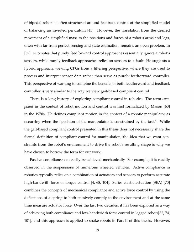
of bipedal robots is often structured around feedback control of the simplified model

of balancing an inverted pendulum [43]. However, the translation from the desired

movement of a simplified mass to the positions and forces of a robot’s arms and legs,

often with far from perfect sensing and state estimation, remains an open problem. In

[52], Kuo notes that purely feedforward control approaches essentially ignore a robot’s

sensors, while purely feedback approaches relies on sensors to a fault. He suggests a

hybrid approach, viewing CPGs from a filtering perspective, where they are used to

process and interpret sensor data rather than serve as purely feedforward controller.

This perspective of wanting to combine the benefits of both feedforward and feedback

controller is very similar to the way we view gait-based compliant control.

There is a long history of exploring compliant control in robotics. The term com-

pliant in the context of robot motion and control was first formalized by Mason [60]

in the 1970s. He defines compliant motion in the context of a robotic manipulator as

occurring when the “position of the manipulator is constrained by the task”. While

the gait-based compliant control presented in this thesis does not necessarily share the

formal definition of compliant control for manipulation, the idea that we want con-

straints from the robot’s environment to drive the robot’s resulting shape is why we

have chosen to borrow the term for our work.

Passive compliance can easily be achieved mechanically. For example, it is readily

observed in the suspensions of numerous wheeled vehicles. Active compliance in

robotics typically relies on a combination of actuators and sensors to perform accurate

high-bandwith force or torque control [4, 68, 104]. Series elastic actuation (SEA) [70]

combines the concepts of mechanical compliance and active force control by using the

deflections of a spring to both passively comply to the environment and at the same

time measure actuator force. Over the last two decades, it has been explored as a way

of achieving both compliance and low-bandwidth force control in legged robots[32, 74,

101], and this approach is applied to snake robots in Part II of this thesis. However,

19

the gait-based compliant control presented in Chapter 3 achieves compliant motion

in pipes without torque sensing or series elasticity by treating the robot’s modules as

parallel actuators that contribute to whole body motions.

Our method for estimating gait parameters uses an extended Kalman filter (EKF)

to efficiently estimate the state of the robot. The EKF is widely used in robotics for

system identification and parameter estimation [1, 83]. The state estimator presented

here is similar to a formulation presented previously by our group [75].

2.4.2 State Estimation

Fusing redundant data in robotics systems is a topic with a wealth of prior work [58].

Perhaps the most common method of fusing redundant and complementary sensor

data is the Kalman filter [44], and its non-linear extensions. Our work includes the

implementation of three non-linear variants of the Kalman filter, an extended Kalman

Filter (EKF), an unscented Kalman filter (UKF), and a spherical simplex unscented

Kalman filter (SSUKF). The EKF extends the Kalman filter to non-linear systems by

linearizing the system at the current state estimate at each timestep [11]. The UKF

is a method that attempts to address the problems inherent in linearization. It uses

a deterministic sampling technique that relies on sigma points to directly calculate the

mean and covariance statistics that are necessary for the filter [40]. The SSUKF is

a variant of the UKF that uses fewer sigma points, making it more computationally

efficient [8, 39].

All forms of Kalman filters have problems in the presence of outliers, due to their

underlying assumption of Gaussian noise in the state estimate and measurement ob-

servations. This is particularly problematic in robotics, where real-world effects like

unmodelled disturbances, faulty sensors, or failed actuators can frequently produce

outliers. Because of this, there has been significant prior work in modifying the Kalman

20

filter to make it more robust to outliers, at the cost of more computation and complex-

ity. Some techniques require noise to be modeled as heavy-tailed distributions [81].

Others use a weighted least-squares approach to learning the state and noise models

online [15]. Ting et al [90] have developed a Kalman filter that is robust to outliers

and requires very little tuning. However, their method relies on estimating the lin-

ear system dynamics, and in our case we have time-varying non-linear process and

measurement models.

Perhaps the most widely used methods of outlier detection are ones that threshold

on the Mahalanobis distance of the measurement residual, or innovation, during a

Kalman filter update [89, 90]. If the Mahalanobis distance is sufficiently large, the

measurement vector at the current iteration is assumed to contain outliers, and the

update step is skipped. Tuning this threshold can be difficult, especially in systems

that are highly dynamic or modeled poorly. Furthermore, instead of skipping the filter

update altogether, we would like to identify individual outliers in the measurement

vector and proceed normally once those are removed. We accomplish both of these

tasks by using the aggregated statistics from all of our robot’s redundant sensors to

automatically adjust a Mahalanobis distance threshold.

2.4.3 Pipe Navigation

There is prior work for design robots to navigate pipe networks. Specialized robots

with wheels have been developed for pipeline inspection [41, 100]. While these robots

advance the state of the art in pipe inspection with their ability to negotiate bends and

junctions, they are specifically designed for specific classes of pipe (freshwater, sewer,

gas) and narrow ranges of pipe diameters. Snake robots offer the ability to adapt to

wide range of diameters and pipe configurations with a single mechanism.

Along these lines, Wakimoto [99] and Kuwada [53] developed snake robots and

21

controllers that use a planar sine-wave gait to push against pipes and negotiate bends

in a lab environment. Our mode of locomotion differs in that we use a helical motion,

which provides greater traction and locomotion compared to planar motions. Further-

more, our tests will be carried out both in the lab and real-world sewer pipes.

22

Chapter 3

Gait-Based Compliant Control

Despite having a powerful low-dimensional control framework for commanding mo-

tions for our snake robots, closing the loop using this framework has proved to be

difficult. To generate motions for the robot, the desired joint angles for each module

are determined from the specified gait parameters at each timestep. Each module in

the robot contains a low-level controller that drives its joint angle to the commanded

angle, and feedback is provided on the module’s actual joint angle [102]. We achieve

limited compliance with our snake robots by using low proportional gains on our in-

dividual modules.

The challenge comes in finding an effective way to incorporate this low-level feed-

back into our higher-level gait-based control. In a sense, we need to find a way in

which the low-level errors of individual joints can ‘complain’ in a meaningful way to a

higher-level controller built around gait parameters that specify whole-body motions.

This work closes the loop by running gait functions in reverse - given a set of joint

angles, we fit a parameterized gait function that best describes the shape of the robot.

We accomplish this by using an EKF to fit gait parameters to joint angle feedback in

real-time.

Gait-based feedback informs the controller of the state of the robot in a language

23

Figure 3.1: Montage of the snake robot using gait-based compliant control to autonomouslynegotiate a transition while climbing up from a 5 cm (2 in) pipe to 10 cm (4 in) pipe. This kindof autonomous behavior goes beyond what even a skilled operator can achieve.

that it (and the operator) understands, gait parameters. By prescribing simple control

laws on gait parameters, we can now create motions that are adaptive to the envi-

ronmentally constrained state of the robot. Furthermore, these controllers allow us to

explore a richer variety of gaits, since a human operator no longer has to be in direct

control of each individual gait parameter.

We demonstrate the effectiveness of this control method with motions that are de-

signed for locomoting along pipes. In our experiments, we show that these controllers

can extend the capabilities of these gaits beyond what has been previous achieved via

remote control. By controlling different gait parameters automatically, the robot is able

to climb a pipe that gradually decreases in diameter and safely stop its motion when

it meets outside resistance like encountering a blockage or being held in place by hand

as shown in Fig. 3.6. Notably, this adaptive behavior is compliant enough that it can

24

provide enough force to climb without over-tightening or being unsafe for human con-

tact. The proposed control framework can also execute gaits that have many more

parameters than a human operator could control. We use a new, more sophisticated,

gait to reliably climb a pipe that undergoes large changes in diameter (Fig. 3.1). Links

to videos demonstrating the compliant controller in action can be found in Appendix

C.

3.1 Compliant Control

The general strategy for gait-based compliant control can be applied to any system

where a low-dimensional controller coordinates the macroscopic shape of a higher

DOF system. In the case of snake robots driven by parameterized gaits, we are essen-

tially fitting a curve, extracting parameters of that curve, and using those parameters

to command new parameters. For the purposes of demonstration, the examples in this

chapter show how this method can be used to automatically control the parameters of

an existing gait used to navigate straight pipes.

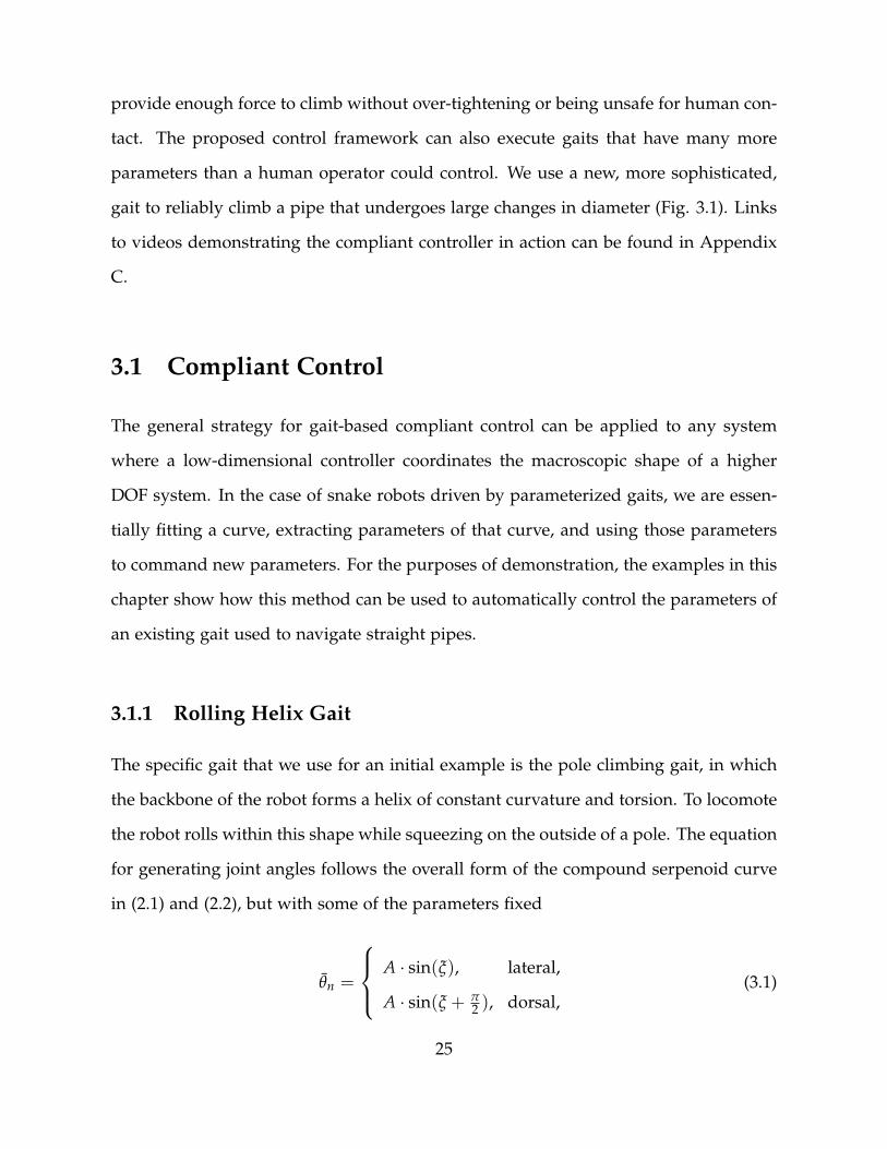
3.1.1 Rolling Helix Gait

The specific gait that we use for an initial example is the pole climbing gait, in which

the backbone of the robot forms a helix of constant curvature and torsion. To locomote

the robot rolls within this shape while squeezing on the outside of a pole. The equation

for generating joint angles follows the overall form of the compound serpenoid curve

in (2.1) and (2.2), but with some of the parameters fixed

θn =

A · sin(ξ), lateral,

A · sin(ξ + π2 ), dorsal,

(3.1)

25

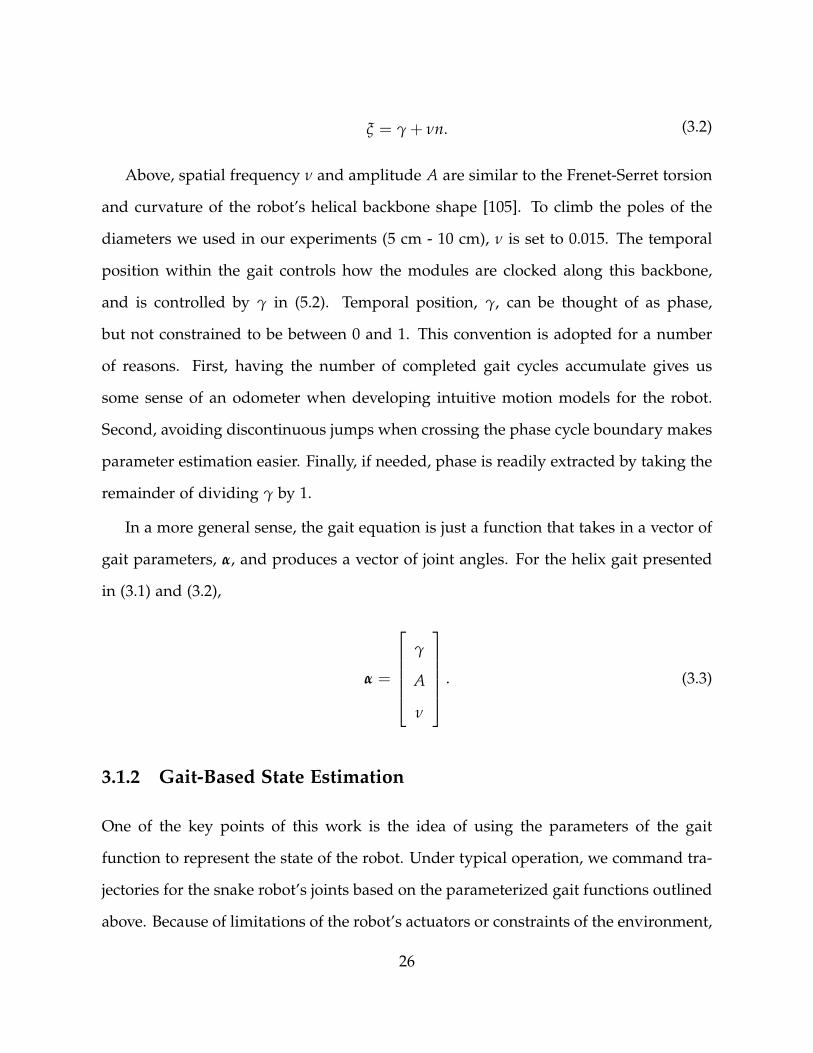
ξ = γ + νn. (3.2)

Above, spatial frequency ν and amplitude A are similar to the Frenet-Serret torsion

and curvature of the robot’s helical backbone shape [105]. To climb the poles of the

diameters we used in our experiments (5 cm - 10 cm), ν is set to 0.015. The temporal

position within the gait controls how the modules are clocked along this backbone,

and is controlled by γ in (5.2). Temporal position, γ, can be thought of as phase,

but not constrained to be between 0 and 1. This convention is adopted for a number

of reasons. First, having the number of completed gait cycles accumulate gives us

some sense of an odometer when developing intuitive motion models for the robot.

Second, avoiding discontinuous jumps when crossing the phase cycle boundary makes

parameter estimation easier. Finally, if needed, phase is readily extracted by taking the

remainder of dividing γ by 1.

In a more general sense, the gait equation is just a function that takes in a vector of

gait parameters, α, and produces a vector of joint angles. For the helix gait presented

in (3.1) and (3.2),

α =

γ

A

ν

. (3.3)

3.1.2 Gait-Based State Estimation

One of the key points of this work is the idea of using the parameters of the gait

function to represent the state of the robot. Under typical operation, we command tra-

jectories for the snake robot’s joints based on the parameterized gait functions outlined

above. Because of limitations of the robot’s actuators or constraints of the environment,

26

the actual joint angles rarely match these commands. Here we show that by fitting the

same parameterized gait functions that we use to generate commanded joint angles to

the feedback joint angles (Fig. 3.2) we can approximately describe the robot’s actual

shape in the more intuitive and lower-dimensional space of gait parameters.

Viewed from a filtering perspective, we can consider the parameters of a gait as a

state that can be repeatedly estimated given some sort of measurement, which in our

case will be the robot’s feedback joint angles. To perform this estimation, we could use

any number of recursive least-squares techniques, and for our work we chose to use

an extended Kalman filter (EKF).

The EKF uses two functions to iteratively update the robot’s estimated state. The

first function is the process model that predicts a new state, xk, given the previous

state, xk−1, and the discrete timestep, ∆t. Our implementation of the EKF performs

updates at a rate of 20 Hz, the same rate as the feedback rate from the robot,

xk = f (xk−1, ∆t). (3.4)

Here, we more formally define the state vector to consist of all the gait parameters,

α, and their first derivatives, α,

x =

α

α

. (3.5)

At each timestep of the filter, the process model forward integrates the gait param-

eters based on the current estimated velocity for each parameter. The model predicts

the gait parameter derivatives to be a mixture of the estimated value from the last

timestep and the commanded velocity,

αk|k−1 = αk−1|k−1 + ˆαk−1|k−1∆t (3.6)

27

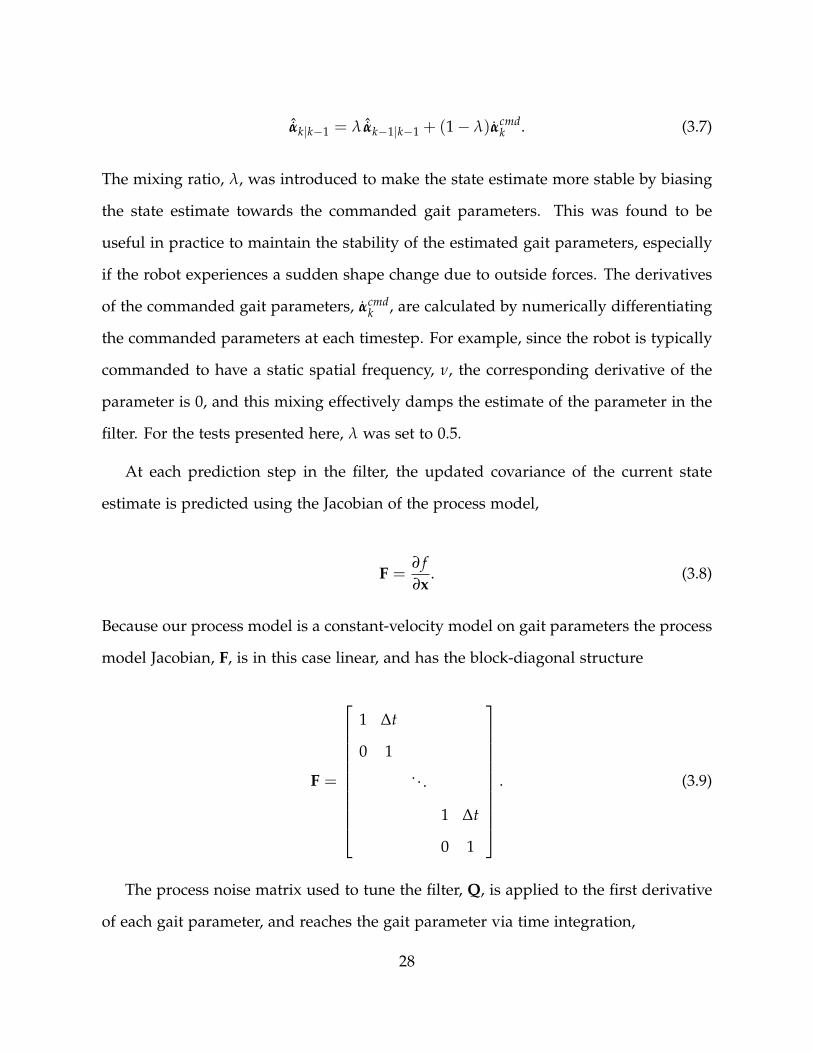
ˆαk|k−1 = λ ˆαk−1|k−1 + (1− λ)αcmdk . (3.7)

The mixing ratio, λ, was introduced to make the state estimate more stable by biasing

the state estimate towards the commanded gait parameters. This was found to be

useful in practice to maintain the stability of the estimated gait parameters, especially

if the robot experiences a sudden shape change due to outside forces. The derivatives

of the commanded gait parameters, αcmdk , are calculated by numerically differentiating

the commanded parameters at each timestep. For example, since the robot is typically

commanded to have a static spatial frequency, ν, the corresponding derivative of the

parameter is 0, and this mixing effectively damps the estimate of the parameter in the

filter. For the tests presented here, λ was set to 0.5.

At each prediction step in the filter, the updated covariance of the current state

estimate is predicted using the Jacobian of the process model,

F =∂ f∂x

. (3.8)

Because our process model is a constant-velocity model on gait parameters the process

model Jacobian, F, is in this case linear, and has the block-diagonal structure

F =

1 ∆t

0 1. . .

1 ∆t

0 1

. (3.9)

The process noise matrix used to tune the filter, Q, is applied to the first derivative

of each gait parameter, and reaches the gait parameter via time integration,

28

Q =∫ ∆t

0F(τ)Ψ FT(τ) dτ. (3.10)

Carrying out this integration yields,

Q =

ψ1∆t3

30 ψ1

∆t2

20

. . . . . .

0 ψn∆t3

30 ψn

∆t2

3

ψ1∆t2

20 ψ1∆t 0

. . . . . .

0 ψn∆t2

20 ψn∆t

. (3.11)

In (3.10), Ψ is a diagonal matrix with the individual noise parameters, ψ1 . . . ψn, that

get applied to the first derivatives, α. In (3.11), the zeros represent upper and lower

triangular sections of zeros that fill out their corresponding matrix block. Instead of

adding process noise individually to the entire state vector, this formulation reduces

the number of tuning parameters by half, correctly accounts for the amount of time

between prediction steps, and adds uncertainty to the appropriate off-diagonals of the

covariance matrix [111]. The values for the noise variables ψi were tuned by hand

and set to between 10−2 and 10−5 and have units that match their corresponding gait

parameters squared.

The second function in the EKF is the measurement model that generates expected

sensor measurements for the robot, zk, given the current prediction of the robot’s state,

xk|k−1,

zk = h(xk|k−1). (3.12)

In the measurement model, the expected joint angles of the robot’s m modules are

generated from the non-linear gait equations (5.4) - (5.5) using the current timestep’s

29

1 3 5 7 9 11 13 15−1

−0.5

0

0.5

1

module number

angle

(ra

d)

Lateral Joint Angles

2 4 6 8 10 12 14 16−1

−0.5

0

0.5

1

module number

angle

(ra

d)

Dorsal Joint Angles

Figure 3.2: Fitting a parameterized gait to joint angle feedback. The blue circles are actual jointangles from the robot. The red curve is the gait function fit to the robot’s joint angles.

estimated gait parameters, α,

z = [ θ1, . . . , θm ]T. (3.13)

Each time the filter performs a measurement update, the innovation covariance is

calculated using the Jacobian of the measurement model,

H =∂h∂x

(3.14)

and the additive measurement noise matrix R.

The measurement noise represents uncertainty in the snake’s joint angle encoders

and is assumed to be independent and of the same magnitude on each joint. For our

robot, we set R to a diagonal matrix with a value of .0001 radians2 on its diagonal,

based on the approximate uncertainty of our joint angle encoders.

30

1 3 5 7 9 11 13 15−1

−0.5

0

0.5

1

module number

angle

(ra

d)

Lateral Joint Angles

2 4 6 8 10 12 14 16−1

−0.5

0

0.5

1

module number

angle

(ra

d)

Dorsal Joint Angles

Figure 3.3: Curvature compliance, where the commanded function (green dashed line) is inphase with the estimated state of the robot (red line), but has a larger amplitude relative theestimated amplitude. The feedback joint angles from the robot (blue dots) are also shown.

3.1.3 Controller

As the environment deforms the robot, compliant control of the robot is achieved

by continually commanding gait parameters that are offset from the current estimated

state. For the following examples, let αcmd be the vector of commanded gait parameters,

αcmd =

γcmd

Acmd

νcmd

. (3.15)

Under normal circumstances all of these parameters would have to be continuously

adjusted by a human operator. The following sections detail the implementation and

resulting behaviors of controlling different parameters compliantly.

31

3.1.4 Curvature Compliance

An example of a simple controller is ‘amplitude compliance’ where the base amplitude

of the robot’s helical curvature is controlled to compliantly squeeze a pipe to maintain

traction as its diameter changes. The controller itself is extremely simple. The com-

manded amplitude, Acmd, is just a constant offset from the estimated amplitude, A,

Acmd = A + ρ. (3.16)

If ρ > 0, the curvature of the overall helical shape of the robot will be increased,

having a tightening effect until the environment constrains the shape the robot, and

results in a controlled ‘squeeze’ on the pipe. This is intuitively illustrated in Fig. 3.3.

The amount of force the robot exerts on pipe is determined by the value of ρ. Choosing

ρ < 0 means the curvature of the robot will be commanded to decrease relative to the

robot’s current curvature. This is useful for motions where the robot climbs something

extremely narrow, like the cable in Fig. A.1. Choosing ρ = 0 results in the curvature of

the robot’s shape complying with whatever outside forces act on it.

3.1.5 Position Compliance

The second controller, (3.17), is ‘position compliance’ where the temporal position of

the gait is controlled so that the robot adapts to resistance that it meets progressing

forward in the gait cycle. For example, if the robot is climbing the outside of a pipe and

encounters a T-junction, this controller allows the robot to safely slow to a stop rather

than continue to roll forward in an open-loop fashion. The commanded temporal

position in the gait, γcmd, is again just a constant offset from the estimated position, γ,

γcmd = γ + ρ. (3.17)

32

1 3 5 7 9 11 13 15−1

−0.5

0

0.5

1

module number

angle

(ra

d)

Lateral Joint Angles

2 4 6 8 10 12 14 16−1

−0.5

0

0.5

1

module number

angle

(ra

d)

Dorsal Joint Angles

Figure 3.4: Position compliance, where the commanded function (green dashed line) is shiftedin phase with the estimated state of the robot (red line). The feedback joint angles from therobot (blue dots) are also shown.

In this controller a positive offset, ρ > 0, causes the robot to drive forward in the

gait cycle, while a negative offset causes it to drive backwards. The larger the offset,

the harder the robot tries to push forward. The effect of this temporal offset in the

commanded joint angles of the robot for pipe crawling is intuitively illustrated in Fig.

3.4.

3.2 Experiments

Experiments were run to test compliant control in both amplitude and temporal posi-

tion. Given good initial parameter estimates, the EKF was observed to be extremely

stable and insensitive to the tuning of the process and and measurement noise param-

eters.

33

16 17 18 19 20 21 22 23 24 25 261

1.1

1.2

1.3

1.4

1.5

1.6

time (sec)

gait

ampl

itude

(rad

)

Gait Amplitude During Pole Climbing Transition

Estimated Gait AmplitudeCommanded Gait Amplitude

Figure 3.5: A montage of the snake robot autonomously transitioning from 4 inch (10 cm)pipe to 2 inch (5 cm) pipe. The green dashed line is the commanded amplitude which is aconstant offset of the estimated amplitude of the gait. While the operator could possibly haveexecuted this transition by starting the robot off with a significantly tighter curvature, the useof compliant is more energy efficient and handles the transition much more robustly.

3.2.1 Curvature Compliance

Curvature compliance in pole climbing was accomplished by commanding an open-

loop velocity in the gait’s temporal position while running the compliant controller on

the amplitude of the gait’s curvature. A compliance offset ρ = 0.1 was used. This

provided enough strength to grip the pole, without straining the modules too much,

and allows vertical climbing on PVC pipes that range in diameter from 5cm to 15cm.

Figure 3.5 shows a montage of the robot making this transition from 10 cm pipe to 5 cm

pipe, along with a plot of the gait’s estimated and commanded amplitudes over time.

As the robot progresses up the pipe, it automatically adapts to the smaller diameter.

3.2.2 Position Compliance

Position compliance in pole climbing was accomplished by running the compliant con-

troller on the gait’s amplitude and position. The compliance offset for amplitude was

the same as the previous experiment. A position compliance offset ρ = .05 was used.

This value was large enough for the robot to climb against the force of gravity, but small

34

13 14 15 16 17 18 19 20 21 22 232.5

3

3.5

4

4.5

time (sec)

gait

posi

tion

(cyc

les)

Gait Position During Pole Climbing

Estimated Gait PositionCommanded Gait Position

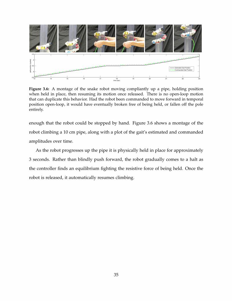
Figure 3.6: A montage of the snake robot moving compliantly up a pipe, holding positionwhen held in place, then resuming its motion once released. There is no open-loop motionthat can duplicate this behavior. Had the robot been commanded to move forward in temporalposition open-loop, it would have eventually broken free of being held, or fallen off the poleentirely.

enough that the robot could be stopped by hand. Figure 3.6 shows a montage of the

robot climbing a 10 cm pipe, along with a plot of the gait’s estimated and commanded

amplitudes over time.

As the robot progresses up the pipe it is physically held in place for approximately

3 seconds. Rather than blindly push forward, the robot gradually comes to a halt as

the controller finds an equilibrium fighting the resistive force of being held. Once the

robot is released, it automatically resumes climbing.

35

36

Chapter 4

Robust State Estimation

To help provide better feedback and improve an operator’s situational awareness, we

have integrated MEMS accelerometers and gyros into each module of our snake robots.

Prior work from our group has already used an extended Kalman filter (EKF) to fuse

these distributed sensors and achieve an estimate of the robot’s pose [76]. By using

knowledge of the robot’s cyclic controller (gait) and taking advantage of an averaged

body frame that we call the virtual chassis, we have been able to estimate a snake robot’s

orientation, even when it undergoes highly dynamic motions.

Unfortunately, our previous work has limitations in terms of its robustness in real-

world field use. Frequent communication dropouts or corrupted data from the mod-

ules would sometimes cause the EKF to diverge. Additionally, the need for the state

estimator to have explicit knowledge of the robot’s gait equation means that it has to

be tightly integrated with the gait framework that we use for control. This work ad-

dresses these issues with two contributions. First, we formulate the state estimation

problem in a way that leverages redundancies in the proprioceptive information pro-

vided by the robot’s joint angle encoders and inertial sensors. In particular, we are able

to redundantly estimate the robot’s kinematic state, the angles, angular velocities, and

angular accelerations of the robot’s joints) by using the inertial sensors in each module

37

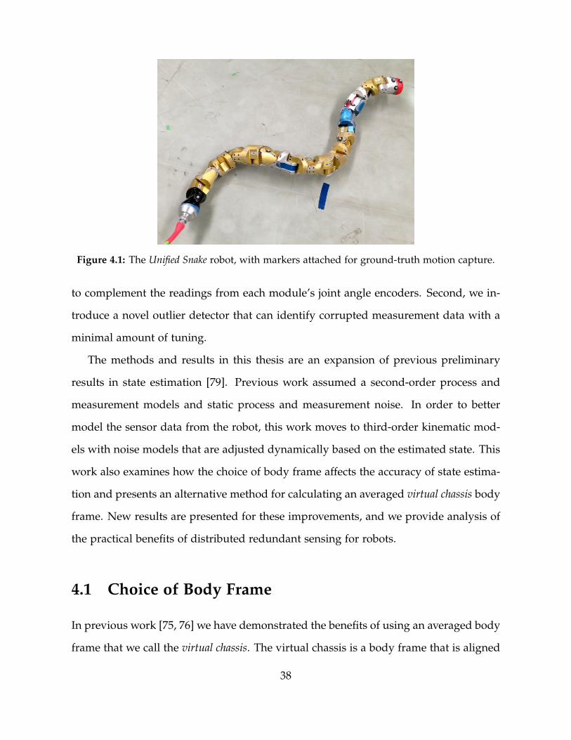
Figure 4.1: The Unified Snake robot, with markers attached for ground-truth motion capture.

to complement the readings from each module’s joint angle encoders. Second, we in-

troduce a novel outlier detector that can identify corrupted measurement data with a

minimal amount of tuning.

The methods and results in this thesis are an expansion of previous preliminary

results in state estimation [79]. Previous work assumed a second-order process and

measurement models and static process and measurement noise. In order to better

model the sensor data from the robot, this work moves to third-order kinematic mod-

els with noise models that are adjusted dynamically based on the estimated state. This

work also examines how the choice of body frame affects the accuracy of state estima-

tion and presents an alternative method for calculating an averaged virtual chassis body

frame. New results are presented for these improvements, and we provide analysis of

the practical benefits of distributed redundant sensing for robots.

4.1 Choice of Body Frame

In previous work [75, 76] we have demonstrated the benefits of using an averaged body

frame that we call the virtual chassis. The virtual chassis is a body frame that is aligned

38

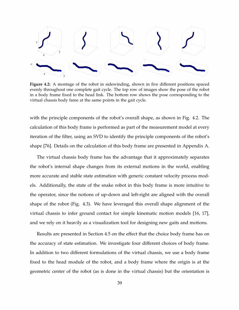
Figure 4.2: A montage of the robot in sidewinding, shown in five different positions spacedevenly throughout one complete gait cycle. The top row of images show the pose of the robotin a body frame fixed to the head link. The bottom row shows the pose corresponding to thevirtual chassis body fame at the same points in the gait cycle.

with the principle components of the robot’s overall shape, as shown in Fig. 4.2. The

calculation of this body frame is performed as part of the measurement model at every

iteration of the filter, using an SVD to identify the principle components of the robot’s

shape [76]. Details on the calculation of this body frame are presented in Appendix A.

The virtual chassis body frame has the advantage that it approximately separates

the robot’s internal shape changes from its external motions in the world, enabling

more accurate and stable state estimation with generic constant velocity process mod-

els. Additionally, the state of the snake robot in this body frame is more intuitive to

the operator, since the notions of up-down and left-right are aligned with the overall

shape of the robot (Fig. 4.3). We have leveraged this overall shape alignment of the

virtual chassis to infer ground contact for simple kinematic motion models [16, 17],

and we rely on it heavily as a visualization tool for designing new gaits and motions.

Results are presented in Section 4.5 on the effect that the choice body frame has on

the accuracy of state estimation. We investigate four different choices of body frame.

In addition to two different formulations of the virtual chassis, we use a body frame

fixed to the head module of the robot, and a body frame where the origin is at the

geometric center of the robot (as is done in the virtual chassis) but the orientation is

39

Figure 4.3: An example of the virtual chassis body frame for various shapes of the snakerobot. Because the body frame is aligned with the principle components of the robot’s shape,it helps separate the robot’s internal shape changes from its external motions, improving theperformance of lower-fidelity models for state estimation.

fixed to the orientation of the head module.

4.2 State Estimation

Snake robots are unique in both their locomotive capabilities as well as their challenges

to estimation and control. Previous work from our group demonstrated accurate esti-

mation of a snake robot’s orientation using the robot’s proprioceptive sensors [79]. To

explore more state of the art techniques, we implemented a UKF and a SSUKF in addi-

tion the conventional EKF, although we found that all three methods worked equally

well. All three filters used the same process and measurement models, as well as the

same values for process and measurement noises. An additional modification from

[79] is that this work moves from a second-order to third-order model for the robot’s

process and measurement models.

40

4.2.1 Kalman Filter

All of the filters presented in this thesis extend the Kalman filter to non-linear systems.

At the heart of the filter are the state estimate, xk, its covariance, Pk, the robot’s sensor

measurements, zk, and the non-linear process and measurement models. The process

model, f , is a function that predicts the state of the robot given the state at a previous

timestep,

xk|k−1 = f (xk−1|k−1, ∆t). (4.1)

The measurement model, h, is a function that generates expected sensor measurements,

zk, given the predicted state xk|k−1,

zk = h(xk|k−1). (4.2)

In the EKF, the state estimate is propagated through these non-linear functions, and

the functions are linearized at each iteration of the filter, resulting in the Jacobians Fk

and Hk that are first-order approximations of the functions f and h. This allows the

propagation of the state covariance between timesteps and the processing of measure-

ments into the state estimate.

In the UKF and SSUKF, a deterministically sampled set of states, called sigma

points, are chosen, propagated through the models, and then averaged in a way that

directly calculates the state mean and covariance. For an n-dimensional state vector,

the UKF uses 2n + 1 sigma points, and the SSUKF uses n + 2 sigma points.

In all of these filters, a process noise matrix, Q, is added to the state covariance at

every prediction step. A measurement noise matrix, R, is similarly used to tune the

confidence in sensor measurements. The parameters in Q and R are used to tune the

relative confidence of different states and measurements with respect to each other.

41

The process model noise for all of the filter variants in this thesis is assumed to be

additive, and is incorporated before the state covariance is pushed through the process

model at each iteration. In both the EKF [111] and the UKF [51], this allows uncertainty

to be added only to the highest derivatives of state variables, relying on the process

model to appropriately distribute uncertainty to the lower derivatives.

4.2.2 State Vector

The state of the filter tracks the robot’s orientation, its inertial frame acceleration, and

its shape variables,

xk = [ ak qk ωk ωk θk θk θk ]T (4.3)

where a = [ ax ay az ] is robot’s world frame acceleration, q = [ q1 q2 q3 q4 ] is the

quaternion that describes the world frame orientation, ω = [ ωx ωy ωz ] is the robot’s

body frame angular velocity, and ω = [ ωx ωy ωz ] is the robot’s body frame angular

acceleration.

For the rest of the state vector, assume a robot with m links with corresponding

joint angles, θ = [ θ1, . . . , θm ], velocities, θ = [ θ1, . . . , θm ], and accelerations, θ =

[ θ1, . . . , θm ]. This provides a third-order description of how the robot’s shape changes

over time.

Because the measurement model that generates expected IMU measurements re-

quires the robot’s full kinematic state, including the robot’s joint angles, velocities, and

accelerations in the state vector means that the filter can iterate at every timestep, even

if the robot does not report all (or even any) of its joint angles at a given timestep. Fur-

thermore, this formulation of the state means the the joint angles are being redundantly

estimated both directly, by observing the joint angles, and indirectly, by observing the

inertial readings at adjacent modules. For example, the gravity vectors observed by the

42

accelerometers in two adjacent modules can indicate the joint angle of a module, and

the difference in angular velocities observed by the gyros in adjacent modules observe

a module’s joint angular velocity. In the Section 4.5, we show that this allows us to

track the angles of modules that fail to provide feedback, even for extended periods of

time.

4.2.3 Process Model

The process model we use for state estimation can be thought of as a generic damped

acceleration model that does not explicitly model the interaction of the world. As a

third-order model, the highest-order derivative in the state is acceleration.

Acceleration is estimated in a world frame assumed to be damped according to

ak = e−τ∆tak−1. (4.4)

In our experience acceleration must be strongly damped (τ ≈ 20) for the filter to per-

form well on the real robot. We should note that this damping was necessary for

estimating the linear acceleration largely because it is extremely difficult to separate

out linear acceleration from sensed acceleration acceleration due to gravity using only

IMUs. The combination of noisy accelerometers, having only an approximate estima-

tion of orientation, and the fact that gravitational acceleration is typically an order of

magnitude greater than linear acceleration means that the estimate of acceleration is

usually quite poor. Solutions to this problem usually rely on well-identified models,

extremely accurate IMUs, particularly gyros, or observing the robot’s linear position

or velocity with a visual sensor or motion capture system.

Previous versions of our state estimators [75] actually assumed zero world frame ac-

celeration of the robot. Ignoring body frame acceleration resulted in good performance

at slow speeds, but became problematic when the snake robot executed fast motions.

43

We have found that this damped third-order model provides a tunable compromise

between a stable but biased second-order model and the more technically accurate but

often unstable third-order model. The estimate of angular acceleration did not need to

be damped, since the numerous gyros in the robot directly observe the robot’s angular

velocity.

The quaternion, qk, representing the orientation of the robot is updated based on

the estimated angular velocities at that timestep. We perform a discrete-time update

developed by van der Merwe et al. [97]

qk = exp(−12

Ψ∆t) qk−1 (4.5)

Ψ =

0 ωx ωy ωz

−ωx 0 −ωz ωy

−ωy ωz 0 −ωx

−ωz −ωy ωx 0

. (4.6)

The body frame angular velocities of the robot, ω, are assumed to update according

to the body frame angular accelerations, and the body frame angular accelerations are

assumed to be constant across timesteps,

ωk = ωk−1 + ˆωk−1∆t (4.7)

ˆωk = ˆωk−1. (4.8)

The shape of the robot is also estimated in the state of the filter. This is achieved by

estimating the snake robot’s joint angles, θ, their angular velocities, ˆθ, and their angular

44

accelerations, ˆθ. These are updated by according to standard third-order model,

θk = θk−1 +ˆθk−1∆t +

12

ˆθk−1∆t2. (4.9)

ˆθk =ˆθk−1 +

ˆθk−1∆t. (4.10)

ˆθk =ˆθk−1. (4.11)

The angular velocities of the joints are further modified by a weighted combination

of the estimated velocities from the third-order model integration, ˆθk, and the com-

manded angular velocities at the current timestep, θcmdk ,

ˆθk = (1− λ) ˆθk + λθcmdk . (4.12)

Even though ˆθk is modified in this equation we have overloaded the notation, since

the filter could be run without this step if commands are unavailable. The weighting

parameter λ ranges from 0 to 1 and controls how much of the commanded angular

velocity is mixed into the state. A value of 1 essentially overwrites the estimated joint

angle velocities at each iteration, whereas a value of 0 turns the filter into a constant-

velocity model that has no knowledge of the robot’s controls. Since the robot’s joints

often deviate significantly from their commanded trajectories, this parameter is set

relatively low, around 0.25.

4.2.4 Measurement Vector

Our latest snake robot provides feedback measurements from single-axis joint angle

encoders, 3-axis accelerometers and a 3-axis gyros located in each module. This means

that the vector of measurements in the filter has 7m dimensions, where m is the total

number of modules in the robot,

45

zk = [ φk αk γk ]T. (4.13)

In (4.13), each element is a vector containing the measurements of a corresponding

sensor type for all the modules throughout the snake robot. φ is the robot’s joint angle

measurements from its encoders, α is the accelerometer measurements, and γ is the

gyroscope measurements.

4.2.5 Measurement Model

Our measurement model is a kinematic model that takes into account the robot’s shape

variables and its inertial state. In the following section, the superscript i indicates the

module for which a measurement is predicted and the hat operator denotes a predicted

measurement, rather than a sensed measurement from the robot.

Expected joint angle measurements are predicted directly from the estimated angles

in the state vector (4.3),

φk = θk. (4.14)

Using the estimated joint angles, θ, and joint angle velocities, ˆθ, joint angle accel-

erations, ˆθ, accelerometer and gyro measurements for each module can be predicted

using the finite time-differencing approach detailed below. This approach allows us to

fuse all of the robot’s IMUs into a single estimate of the robot’s orientation as well as

couple the IMUs to the encoders to redundantly estimate the robot’s shape.

Accelerometers have the property that they measure an acceleration due to gravity

in addition to lateral acceleration due to motion. For this reason our model treats

these two sources of acceleration separately and sums them to generate the predicted

accelerometer measurement for each module,

46

αik = ai

gravity + aimotion. (4.15)

Acceleration due to gravity is predicted by transforming the estimated gravity vector

g from the world frame into the frame of each module

aigravity = (Wi

k)T(Vk)

Tg (4.16)

where Wi is the estimate of the rotation matrix that describes the orientation of module

i in the body frame, and V is the estimate of the rotation matrix representation of the

quaternion pose q in the state vector (4.5).

Acceleration due to a module’s motion is further split into two components,

aimotion = ai

internal + (Wik)

T(Vk)Ta (4.17)

Acceleration due to the robot’s internal shape changes in the body frame, aiinternal,

is predicted by double-differentiating the position of the module in the body frame,

based on the full kinematic state. Finally, the estimated world frame acceleration of

the entire robot is incorporated by rotating the world frame acceleration a from filter’s

state estimate into the frame of each module.

The predicted gyro measurements for each module are generated by differentiating

the orientation of the robot at two nearby timesteps [63]. If Wik and Wi

k−1 are rotation

matrices that describe the orientations of module i in the body frame at two timesteps,

then gyro measurements due to the robot’s motion in the body frame at two timesteps,

47

k and k− 1 can be approximated by

1 −ωiz ωi

y

ωiz 1 −ωi

x

−ωiy ωi

x 1

≈

Wik(W

ik−1)

T

∆t. (4.18)

The complete prediction for each gyro is the angular velocity from (4.18) plus the

robot’s body frame angular velocity from the current state estimate, (4.8), rotated into

the coordinate from of each module using Wik

γik = ωi + (Wi

k)Tωk. (4.19)

This finite-differencing approach has allowed us to generate expected readings for all

of the robot’s IMUs and encoders, based on the current state estimate, x. While our

numerical approach somewhat computationally expensive, this part of the measure-

ment model has been implemented in C++ using the Eigen matrix library, allowing the

remaining sections of the filter to run in Matlab, in real time, on a standard desktop

computer.

4.2.6 State-Based Noise Adjustment

To improve the accuracy of the Gaussian noise assumption for the models and sensors,

the additive process and measurement noise matrices, Q and R, are modified based on

the current state estimate. Intuitively, if the robot is moving, the model should be less

certain about the current estimate than if the robot is standing still. This matches real-

world observation, where it can be readily observed that readings from the robot’s

sensors, particularly the accelerometers, are much noisier during fast motions than

when the robot is still or moving slowly.

48

The process noise parameters are inflated based on the current state estimate and

corresponding tuning parameters. The block of the process noise matrix corresponding

to body frame angular acceleration, ˆω, is adjusted according to the magnitude of body

frame angular acceleration, ˆω, and body frame angular velocity ω. The additive noise

for joint angle accelerations, ˆθ, are similarly inflated according to the squared value of

the estimated joint angular accelerations, ˆθ, and joint angular velocities, ˆθ.

The measurement noise parameters are also inflated based on the current state esti-

mate. The additive noises for the accelerometers, α, in each module are inflated based

on the magnitude of the gyro measurements for that module. Of all the modifications

in this section, this in particular led to better performance of the filters compared to

our previous work, since the accelerometers become particularly noisy when the robot

is in motion.

4.2.7 Using Partial Measurement Data

Due to noise in the robot’s communications, around 5% of the robot’s sensor data

is missing at a given update step. In the case of intermittent electrical connections

between the modules this percentage can increase even further. Furthermore, when

using the snake robots aggressively in the field, modules frequently reset due to their

electrical protection circuitry. In these cases an individual module may drop out for

2-3 seconds before rebooting. During this time the module’s joint is rotating freely, but

there is no direct measurement of its joint angle. Thus, it is desirable to have a method

that uses the robot’s myriad of other sensors to mitigate these problems.

Missing measurement data can be accommodated in any Kalman filter by only pre-

dicting expected measurements for the observed sensors and appropriately resizing the

innovation covariance matrix during the filter’s update step. An alternative approach

that is simple to implement is one where the missing measurement data is replaced

49

with a value of 0, and that measurement’s corresponding value in the additive mea-

surement noise matrix, R, is increased to 106 for that timestep. This causes the filter

to effectively ignore the measurement during the update step and is often simpler to

implement than dynamically resizing the covariance and state at every iteration.

4.3 Outlier Detection

As mentioned in the previous section, the Kalman filter can be easily modified to ac-

commodate incomplete measurements during its iteration. However, corrupted mea-

surements and outliers that violate the filter’s assumption of Gaussian noise are much

more problematic [89, 90]. In robotic systems that undergo heavy field use, it is not

uncommon for sensors to become unresponsive or miscalibrated. And because these

erroneous measurements from an unresponsive sensor can severely disrupt the state

estimate, it is beneficial to detect such outliers automatically from the observed sensor

data.

4.3.1 Kalman Filter Update

The Kalman filter, and its non-linear variants, updates the estimated state based on a

weighted average that takes into account the measurement innovation, which is the

difference between the expected measurements, zk, generated from the measurement

model, and the observed measurements, zk, from the robot’s sensors,

xk|k = xk|k−1 + Kk(zk − zk),

The proper weighting of the update is determined by the Kalman gain matrix, Kk.

In the calculation of this matrix, there is an intermediate step where the innovation

covariance, Sk, is calculated. The relevant steps in the respective EKF and UKF /

50

SSUKF algorithms are presented here for clarity.

In the linear Kalman filter and the EKF, the innovation covariance and Kalman gains

are determined based on the estimated covariance and the Jacobian of the measurement

model,

Sk = HkPk|k−1HTk + R,

Kk = Pk|k−1HTk S−1

k .

In the UKF and SSUKF, the innovation covariance and Kalman gains are determined

directly from matrices, Pzzk and Pxz

k , derived from the sampled sigma points [39], and

additive measurement noise,

Sk = Pzzk + R,

Kk = Pxzk S−1

k .

The Mahalanobis distance for the residual error between the predicted measure-

ment vector, zk = h(xk|k−1), and the observed measurement vector, zk,

dk = (zk − zk)TS−1

k (zk − zk),

gives an indication of the likelihood of the measurements.

4.3.2 Algorithm

To detect outliers our method computes, for each sensor s, a Mahalanobis distance that

excludes sensor s from the measurement vector. In the following section we will use

51

superscripts −s to clarify that they are quantities where sensor s has been excluded. To

exclude these elements, we define the following selection matrix,

Y−s =

IM×M 0M×3 0M×N

0N×M 0N×3 IN×N

,

where M is the number of elements in the measurement vector zk that precede sensor

−s, N is the number of elements in zk that follow sensor −s, and 3 is the number of

elements in the measurement vector that correspond to sensor −s (the x − y− z axes

of an accelerometer or gyro).

This process of excluding the elements of and calculating the Mahalanobis distance

of the remaining elements of[S−s

k

]−1 incorporates information on how the sensors are

coupled by the process and measurement models. A simpler, more naive, alternative

to this approach would be to calculate the Mahalanobis distance of the 3 × 3 block

of[S−s

k

]−1 corresponding to each sensor directly. This assumes that each sensor is

independent, which in some cases may be an appropriate assumption.

The Mahalanobis distance associated with excluding sensor −s can be written as

follows,

d−sk = (z−s

k − z−sk )T [S−s

k]−1

(z−sk − z−s

k ), (4.20)

where z−sk = Y−szk, z−s

k = Y−szk, and S−sk = Y−sSk(Y−s)T.

For each excluded sensor−s, a Mahalanobis distance d−sk that is significantly smaller

than dk means that the excluded component is likely to be an outlier. Sorting the set

of distances for each sensor ranks the sensor measurements in order of likeliness. We

then discard a fixed number of the least likely sensor measurements (the ones that are

most likely to be outliers) and calculate the mean, µk, and standard deviation, σk, of the

remaining Mahalanobis distances, presumed to be inliers. For our implementation, we

52

choose to discard 4 sensors from the measurement vector, or one quarter of the robot’s

sensors.

Finally, for each sensor −s, a new metric is computed that compares the Maha-

lanobis distance d−sk to the mean and variance of the Mahalanobis distances of the

presumed inliers,

w−sk =

(d−s

k − µk)2

σ2k

.

We then consider all sensors, including the initially discarded sensors, and decide

whether each one is an inlier or outlier by thresholding the metric w−sk at some level, ξ.

When w−sk is large, the sensor is likely to be an outlier and when this metric is small,

the sensor measurement is likely to be an inlier. If the measurement is determined to be

an outlier, the innovation covariance is resized to exclude the measurement, just as is

done for missing data. Alternatively, a simple approximation to dynamically resizing

the measurement innovation is to simply set the measurement’s corresponding element

in R to a comparatively large value, such as 106.

In a sense, w−sk is a Mahalanobis distance of Mahalanobis distances, and is in many

ways akin to data clustering. Since this value is based on the overall uncertainty of

all of similar sensors in the robot, we are able to pick a single static threshold that is

valid at all times. For example, if the process model predicts the state of the robot

poorly, or if the filter is poorly tuned, all of the measurements might have a large

absolute uncertainty. However, this method relies on the relative uncertainty between

measurements to determine outliers.

Compared to thresholding on the Mahalanobis distance alone, outliers with this

method tend to be extremely obvious, often greater than 100 standard deviations from

the mean. Setting the detection threshold, ξ, to a value between 10 and 50 has been

shown to work well for our system, regardless of sensor type or the robot’s motion.

53

Finally, since this algorithm makes the assumption that some fraction of the sensors

must be inliers, it has the benefit that it ensures an upper limit on the number of

sensors that can be discarded as outliers, as long as ξ is not set too low (setting ξ > 3

standard deviations). This allows outlier detection to be performed even when a filter

is still being debugged or is poorly tuned, and the absolute Mahalanobis distances

could be unusually large or small.

4.3.3 Efficient Implementation

One drawback of the outlier detection algorithm, as presented thus far, is the need to

invert S−sk for each sensor in order to compute d−s

k as computed in (4.20). For our 16-

link snake robot that has 2 inertial sensors per module, the accelerometer and the gyro,

performing this for a typical 16-link robot would require 32 inversions of a 109-by-109

matrix. This is a significant computational expense during real-time operation.

Ideally, it would be beneficial to compute the inverse of the innovation covariance,

S−1k , only once and then to somehow efficiently infer, for each sensor s, the matrix[S−s

k

]−1. By definition,[S−s

k

]−1=[Y−sSk(Y−s)T]−1. But unfortunately,

[S−s

k

]−1 6=

Y−sS−1k (Y−s)T, otherwise we would compute

[S−s

k

]−1 directly from S−1k . This is not

possible because Y−s is not an orthogonal matrix.

Instead, we can leverage the Woodbury matrix identity [72], to perform a low-rank

correction to the relatively large matrix S−1k . This allows us to efficiently obtain the

matrix[S−s

k

]−1, which we require for computing the Mahalanobis distance in Eq. (4.20).

First, we define the following matrix that can be used to rearrange the elements of the

innovation so that the elements corresponding with sensor −s are last,

G−s =

←−−−− Y−s −−−−→

03xM I3x3 03xN

,

54

Using this matrix, we can rearrange the inverse of the innovation covariance matrix as

follows,

[S′k]−1 =

[G−sSk(G−s)T

]−1= G−sS−1

k (G−s)T =

A B

BT C

.

Using the Woodbury matrix identity to invert the matrix [S′k]−1, we obtain,

S′k =

(A− BC−1BT)−1 ∼

∼ ∼

.

Above, the ∼ indicates regions of the matrix from the Woodbury matrix identity that

are omitted for clarity. Since the upper left component of S′k is equal to the matrix S−sk ,

due the existence of Y−s in G−s, we can simply invert the upper left component of S′k,

[S−s

k]−1

= A− BC−1BT. (4.21)

In (4.21), C is the inverted covariance of the sensor being excluded. This form

only requires the inversion of C, which in our case is 3-by-3. Thus, we can efficiently

calculate the inverse of the innovation covariance,[S−s

k

]−1 for each test of a sensor s

by performing a small update to the full inverse of the innovation covariance matrix

S−1k . A summary of the algorithm that we use for outlier detection is provided in

Algorithm 1.

4.4 Experiment

To test the accuracy of the different state estimators, multiple trials of the snake robot

were performed in a Vicon motion capture system. During these trials, the robot was

remotely controlled through a wide variety of motions, some of which were quite fast

55

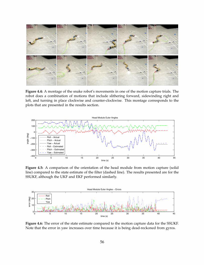
Figure 4.4: A montage of the snake robot’s movements in one of the motion capture trials. Therobot does a combination of motions that include slithering forward, sidewinding right andleft, and turning in place clockwise and counter-clockwise. This montage corresponds to theplots that are presented in the results section.

0 5 10 15 20 25 30 35 40 45−400

−300

−200

−100

0

100

200Head Module Euler Angles

time (s)

an

gle

(d

eg

)

Roll − Actual

Pitch − Actual

Yaw − Actual

Roll − Estimated

Pitch − Estimated

Yaw − Estimated

Figure 4.5: A comparison of the orientation of the head module from motion capture (solidline) compared to the state estimate of the filter (dashed line). The results presented are for theSSUKF, although the UKF and EKF performed similarly.

0 5 10 15 20 25 30 35 40 450

10

20

30Head Module Euler Angles − Errors

time (s)

err

or

(de

g)

Roll

Pitch

Yaw

Figure 4.6: The error of the state estimate compared to the motion capture data for the SSUKF.Note that the error in yaw increases over time because it is being dead-reckoned from gyros.

56

Algorithm 1 Outlier Detection Procedure1: for each −s do2: S′−1

k ← G−sS−1k (G−s)T

3: [A, B, C]← extractBlocks(

S′−1k

)

4:[S−s

k

]−1 ← A− BC−1BT

5: z−sk = Y−szk

6: z−sk = Y−szk

7: d−sk = (z−s

k − z−sk )T [S−s

k

]−1(z−s

k − z−sk )

8: end for9: [µk, σk]← statistics_of_inliers

(d−s

k for all s)10: for each −s do

11: w−sk ←

(d−sk −µk)

2

σ2k

12: if w−sk > ξ then

13: Mark s as outlier14: end if15: end for

and abrupt. The pose of the head module was tracked by the motion capture system

to provide ground truth. This was then compared to the filter’s estimate for pose of

the head module, which is dependent on the estimate of the entire state of the robot.

Figure 4.5 shows a montage of the robot during one of these trials.

To demonstrate the advantages of redundant state formulation, we simulated miss-

ing data and complete module dropouts. To test the outlier detection algorithm, we

simulated corrupted data on the robot’s inertial sensors similar to what is seen when

a module is poorly calibrated or programmed incorrectly.

4.5 Results

Overall, the EKF, UKF and SSUKF performed comparably. The filters were all able

to run in real time on the feedback data coming from the robot, about 20 Hz. A

comparison of the errors of the estimated head module orientation, converted to Euler

angles, for each filter is presented in Table 4.1. This is the averaged error for 3 different

57

Filter Performance ComparisonEuler Angle Errors (degrees)

Roll Pitch YawEKF 3.3 3.9 13.4UKF 3.2 3.8 11.3SSUKF 3.2 3.8 10.9

Table 4.1: The accuracy of various non-linear Kalman filters in estimating the Euler angleorientation of the head module of the snake robot. All of the filters perform comparably.

motion capture trials where the robot was driven in a wide variety of speeds and

directions. The accuracy in yaw is significantly worse than pitch and roll because it is

being dead-reckoned based on the filter’s integration of estimated angular velocities.

Figures 4.5 and 4.6 show a comparison of the estimated head module orientation

from the SSUKF compared the motion capture data for one of the trials. To provide a

meaningful comparison the quaternion orientations of the head have been converted

into Euler angles.

4.5.1 State-Based Noise Adjustment

Table 4.2 shows the performance of the EKF, UKF, and SSUKF without dynamically ad-

justing the process and measurement noises based on the estimated state, as described

in Section 4.2.6. There was no measurable benefit of tuning the noises dynamically

for pitch and roll, and all of the filters performed comparably. However, there was a

significant improvement in the dead-reckoned yaw performance for all of the filters.

We believe this is primarily because the state-based noise adjustment allows the gyros

being trusted more heavily for fast motions, while at the same time trusting the more

noisy accelerometers less.

58

Filter Performance - WithoutDynamic Noise AdjustmentEuler Angle Errors (degrees)

Roll Pitch YawEKF 2.9 3.4 36.3UKF 2.9 3.4 34.7

SSUKF 3.1 3.3 24.3

Table 4.2: The accuracy of the various filters in estimating the orientation of the head moduleof the snake robot, without dynamically adjusted process and measurement noise. The filtersperform similarly as when noises are not dynamically tuned, with the exception that dead-reckoned yaw estimation is significantly worse.

SSUKF Performance - Missing DataEuler Angle Errors (degrees)

Roll Pitch YawBaseline 3.2 3.8 10.925% Missing 3.6 3.9 9.450% Missing 5.6 5.8 26.575% Missing 9.0 11.1 57.5

Table 4.3: The accuracy of the SSUKF in predicting the Euler angle orientation of the headmodule of the snake robot. The filter performs well even with half of the robot’s data beingexcluded. Even when 50% of the data is excluded the filter continues to run well, althoughaccuracy begins to be degraded for larger amounts of feedback loss.

4.5.2 Partial Measurement Data

Under normal circumstances, our snake robot drops about 5% of its data due noise

and errors in its communications. To simulate more adverse conditions, we randomly

selected and removed higher proportions of the robot’s feedback data. The results are

summarized in Table 4.3.

We simulated prolonged module dropouts by eliminating all of the feedback data

(joint angles, gyros, accelerometers) from a module in the robot for the entirety of the

same data set shown in Fig. 4.5 and Fig. 4.6. For the data presented here, the joint

angles and inertial sensors were unavailable for the entire run in modules 3, 6, 7 and

12. Even if up to 4 modules were eliminated the filter still converged and estimated

59

SSUKF Performance - Dropped ModulesEuler Angle Errors (degrees)

Roll Pitch YawBaseline 3.2 3.8 10.9Missing 4 Modules 4.0 4.3 59.1

Table 4.4: The accuracy of the SSUKF in the presence of missing data from multiple modulesfor the entire run. These results are for the same trial as shown in Fig. 4.4. Feedback from aquarter of the snake robot (modules 3,6,7 and 12) was eliminated.

0 5 10 15 20 25 30 35 40 45−50

0

50Actual vs. Estimated Joint Angle for Failed Module

time (sec)

Jo

int

An

gle

(d

eg

ree

s)

Measured Joint Angle

Estimated Joint Angle

Figure 4.7: A comparison of the actual and estimated joint angle for module 7 in the snakerobot. No feedback was available to the filter for modules 3,6,7 and 12 during the entire trial,but the joint angle is able to be estimated from the feedback from the remaining modules.

the pose of the head reasonably well (Table 4.4).

The accuracy of a missing joint angle being estimated by the filter is shown in more

detail by Figs. 4.7 and 4.8. While the error of the estimated joint angle is as much as

10◦ at times, the filter does a reasonable job of estimating the joint angle even while

the robot is undergoing significant motion. It is also worth noting that the estimated

uncertainty of the joint angle is appropriately captured by the filter.

4.5.3 Different Body Frames

Based on our previous experience, we believe that the choice of body frame can effect

the accuracy of state estimation, and as such we ran the SSUKF in four different body

frames. As a baseline comparison, the first body frame was fixed to the head module

60

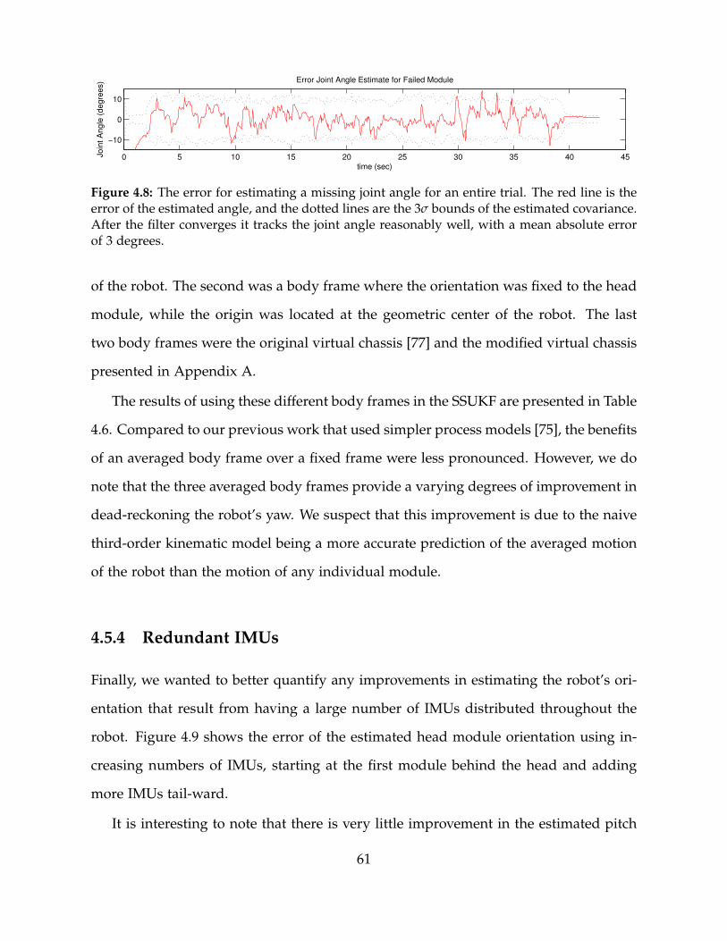
0 5 10 15 20 25 30 35 40 45

−10

0

10

Error Joint Angle Estimate for Failed Module

time (sec)

Jo

int

An

gle

(d

eg

ree

s)

Figure 4.8: The error for estimating a missing joint angle for an entire trial. The red line is theerror of the estimated angle, and the dotted lines are the 3σ bounds of the estimated covariance.After the filter converges it tracks the joint angle reasonably well, with a mean absolute errorof 3 degrees.

of the robot. The second was a body frame where the orientation was fixed to the head

module, while the origin was located at the geometric center of the robot. The last

two body frames were the original virtual chassis [77] and the modified virtual chassis

presented in Appendix A.

The results of using these different body frames in the SSUKF are presented in Table

4.6. Compared to our previous work that used simpler process models [75], the benefits

of an averaged body frame over a fixed frame were less pronounced. However, we do

note that the three averaged body frames provide a varying degrees of improvement in

dead-reckoning the robot’s yaw. We suspect that this improvement is due to the naive

third-order kinematic model being a more accurate prediction of the averaged motion

of the robot than the motion of any individual module.

4.5.4 Redundant IMUs

Finally, we wanted to better quantify any improvements in estimating the robot’s ori-

entation that result from having a large number of IMUs distributed throughout the

robot. Figure 4.9 shows the error of the estimated head module orientation using in-

creasing numbers of IMUs, starting at the first module behind the head and adding

more IMUs tail-ward.

It is interesting to note that there is very little improvement in the estimated pitch

61

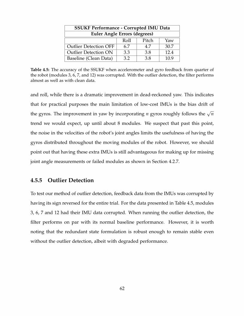
SSUKF Performance - Corrupted IMU DataEuler Angle Errors (degrees)

Roll Pitch YawOutlier Detection OFF 6.7 4.7 30.7Outlier Detection ON 3.3 3.8 12.4Baseline (Clean Data) 3.2 3.8 10.9

Table 4.5: The accuracy of the SSUKF when accelerometer and gyro feedback from quarter ofthe robot (modules 3, 6, 7, and 12) was corrupted. With the outlier detection, the filter performsalmost as well as with clean data.

and roll, while there is a dramatic improvement in dead-reckoned yaw. This indicates

that for practical purposes the main limitation of low-cost IMUs is the bias drift of

the gyros. The improvement in yaw by incorporating n gyros roughly follows the√

n

trend we would expect, up until about 8 modules. We suspect that past this point,

the noise in the velocities of the robot’s joint angles limits the usefulness of having the

gyros distributed throughout the moving modules of the robot. However, we should

point out that having these extra IMUs is still advantageous for making up for missing

joint angle measurements or failed modules as shown in Section 4.2.7.

4.5.5 Outlier Detection

To test our method of outlier detection, feedback data from the IMUs was corrupted by

having its sign reversed for the entire trial. For the data presented in Table 4.5, modules

3, 6, 7 and 12 had their IMU data corrupted. When running the outlier detection, the

filter performs on par with its normal baseline performance. However, it is worth

noting that the redundant state formulation is robust enough to remain stable even

without the outlier detection, albeit with degraded performance.

62

SSUKF Performance - Different Body FramesEuler Angle Errors (degrees)

Roll Pitch YawHead-Fixed Frame 5.4 4.2 17.4Head-Fixed Orientation / COM 4.1 4.1 14.0Virtual Chassis [76] 3.2 3.8 10.0Alternate Virtual Chassis 3.1 3.6 10.8

Table 4.6: The accuracy of various of the SSUKF in estimating the Euler angle orientationof the head module of the snake robot using different body frames for the filter process andmeasurement models. An averaged body frame improves performance slightly, although theamount improvement depends heavily on the nature of the robot’s motion.

2 4 6 8 10 12 14 160

5Errors for Increasing Number of IMUs − Degrees

Ro

ll

Number of Modules Used

2 4 6 8 10 12 14 160

2

4

Pitch

Number of Modules Used

2 4 6 8 10 12 14 160

20

40

60

Ya

w

Number of Modules Used

Figure 4.9: Error of the estimated head module orientation using increasing numbers of IMUsfor the state estimate. Using additional IMUs provides little improvement in the estimation ofpitch and roll, but greatly reduces the dead-reckoning error in yaw.

63

64

Chapter 5

Application: Pipe Network Navigation

Underground sewer pipes were chosen as a target environment to demonstrate the in-

tegration and application of the developments of this thesis. While there are a number

of specialized tools available for the inspection and maintenance of sewer pipes, we set

out to perform tasks that would be difficult for any one tool to accomplish. In partic-

ular, we focused on negotiating the transition between a sewer collector pipe and the

smaller pipe that joins it from a house, called a lateral.

Reliably locomoting through a lateral junction involves integrating state estimation

and compliant control so that a robot’s gait can be adjusted autonomously and based

on an accurate estimate of its orientation in a world frame. It also requires the de-

velopment of new pipe-crawling gait that includes parameters that allow the robot to

navigate pipe bends and junctions.

5.1 Pipe Crawling Gait

The basic pipe crawling gait [88] commands joint angles along the robot’s backbone,

θl, such that the shape of robot forms a helix of constant curvature,

65

θl =

dl(A·sin(ξ)), lateral,

dl(A·sin(ξ + π2 )), dorsal,

(5.1)

ξ = 2π(γ + νl). (5.2)

In (5.1), A is the amplitude of the sinusoidal oscillation for each module. In (5.2) the

parameter ν describes the spatial frequency of the macroscopic shape of the robot with

respect to module position, l. The parameter, l, refers to a normalized snake length

that varies from 0 at the head to 1 at the tail. The temporal position, γ, within the gait

controls the twisting motion of the base shape of the robot about the backbone curve,

which is the main means of locomotion. Since the gait is a cyclic function, temporal

position modulo 1 can be thought of as the phase within the gait cycle. It is also

common to set γ to change with constant velocity,

γ = ωt. (5.3)

Spatial frequency ν and amplitude A are similar, respectively, to the Frenet-Serret

torsion and curvature of the robot’s helical backbone shape [105]. Depending on the

specific value of ν, the robot’s overall helical shape can be designed to move on either

the outside (Fig. 5.1) or the inside (Fig. 5.2) of pipes.

Unlike previous presentations of our gaits, these gait equations are parameterized

in terms of curvatures that have the units of radians / snake length. These curvatures

are multiplied by joint length, dl, to obtain actual joint angles. This modification will

allow the gait parameters to scale more appropriately to robots with different joint

spacing and accommodate future robots that may have non-uniform joint lengths.

To enable the snake robot to actively navigate bends and junctions, we created

a modified version of the helical pipe crawling gait [78, 88]. Specifically, we added

66

0 0.2 0.4 0.6 0.8 1

−1

0

1

normalized snake length

angle

(ra

d)

Lateral Joint Angles

0 0.2 0.4 0.6 0.8 1

−1

0

1

normalized snake length

angle

(ra

d)

Dorsal Joint Angles

Figure 5.1: A configuration of the basic pipe crawling gait (left), used for traveling on theoutside of pipes and poles. The plots to the right show the corresponding lateral and dorsaljoint angles.

a parameterized planar bend to robot’s backbone that could be localized along the

length of the robot and adjusted in its amplitude and direction. This bending mode

was added on top of the base helix shape, resulting in the new gait equations

θl =

dl(Al·sin(ξ) + cos(φ)Aκ ϕ(µ, σ, l)), lateral,

dl(Al·sin(ξ + π2 ) − sin(φ)Aκ ϕ(µ, σ, l)), dorsal,

(5.4)

Al = A(1− ϕ(µ, 2σ, l)). (5.5)

The planar bending mode was created using a Gaussian function, shown in Fig. 5.4,

that was superimposed onto the baseline curvature of the pipe crawling gait, shown

in Fig. 5.2. To ensure that the bend lies in a single plane, the base amplitude of the

helix, A, is tapered to straight line using a second Gaussian function with a width

that is set twice as wide as the bend width (5.5). The net effect of this planar bending

mode is shown in Fig 5.3, where a bending mode is present lateral joint angles and a

straightening effect is observed in the dorsal joint angles. The Gaussian function, ϕ, is

normalized so that the magnitude of the center of the Gaussian is always 1, which is

67

0 0.2 0.4 0.6 0.8 1−1

0

1

normalized snake length

angle

(ra

d)

Lateral Joint Angles

0 0.2 0.4 0.6 0.8 1−1

0

1

normalized snake length

angle

(ra

d)

Dorsal Joint Angles

Figure 5.2: A configuration of the basic pipe crawling gait (left), used for traveling throughstraight pipes. The plots to the right show the corresponding lateral and dorsal joint angles.

then scaled by the bend amplitude, Aκ. The spatial location and width of the Gaussian

are controlled respectively by the parameters µ and σ. The direction of the bend with

respect to the lateral and dorsal planes along the robot’s backbone is controlled by a

specified bend angle, φ. Figure 5.3 shows the robot’s shape with a bend angle of 0◦

creating a bend to the left. Given the same base shape of the robot, a bend angle of

180◦ would create a bend to the right.

Controlling the gait parameters during operation is accomplished in one of three

ways. The first is that the operator manually sets and adjusts the value. Up until now,

this method has been the primary means of control of our snake robots. The second is

that the parameter is controlled compliantly, based on its estimated value. In this case,

the operator commands an offset from the parameter’s estimated value and the system

servos to a sum of the estimated value and this offset. Finally, parameters can be set

automatically via some other process, e.g., the estimated orientation of the robot. The

full set of gait parameter values are detailed in Section 5.3.

When navigating a pipe junction, the operator sets the bend width, σ, to a static

value. For the work presented in here, σ was set to a static value of 0.1. This allowed

the bend to be tight enough to negotiate a sharp 90◦ turn, while being broad enough

68

0 0.2 0.4 0.6 0.8 1−1

0

1

normalized snake length

angle

(ra

d)

Lateral Joint Angles

0 0.2 0.4 0.6 0.8 1−1

0

1

normalized snake length

angle

(ra

d)

Dorsal Joint Angles

Figure 5.3: A configuration of the modified pipe crawling gait, with a bending mode added tothe front of the robot in the lateral plane that causes the head to hook to the left. The plots tothe right show the corresponding lateral and dorsal joint angles.

0 0.2 0.4 0.6 0.8 10

0.5

1

normalized snake length

an

gle

(ra

d)

φ(µ, σ, l)

l

µ

σ

Figure 5.4: The function ϕ that is used to add a bending mode to the pipe crawling gait. Thebend is created by adding a Gaussian that is centered at the position, µ, with a characteristicwidth, σ.

to allow the bend to be present in multiple joints of the robot, which aided in the

stability of the parameter estimation for compliant control, described in the following

section. As the robot drives down a straight pipe and encounters a junction, the op-

erator manually initializes a bend location µ at the head of the robot with an initial

amplitude Aκ. These parameters are controlled compliantly, with the bend location µ

being passed tail-ward along the backbone, and the bend amplitude Aκ complying to

the pipe’s bend geometry, as the robot progresses through the bend.

The bend direction φ is set based on a desired world frame direction (e.g., left,

right, up, down). Because the gait’s bend direction is specified in a frame fixed to

69

the robot, a separate process that estimates the orientation of the robot [79] is used to

determine the body frame direction, φ, that corresponds to the desired world frame

direction. For example, in Fig. 5.3, the curvature of bend is located in the lateral plane

of the robot. If the robot’s orientation rolled by 90◦, the bend would need to be rotated

accordingly, so that the curvature was located in the dorsal plane. Compensating for

this motion based on the orientation of the head module of the robot allows the bend

to be properly oriented at all times, even as the robot corkscrews through the pipe.

5.2 Compliant Controller

To navigate pipe junctions, three gait parameters are controlled compliantly, following

the methods laid out in Chapter 3, by assigning offsets, ρ, from the current parameter

estimate. Compliance on helical curvature, A, of the robot’s helical backbone shape

was used to ensure that the robot pushed out onto the pipe for traction, regardless of

changes in pipe diameter. The bend amplitude, Aκ, and bend position, µ, were also

controlled compliantly with positive offsets to encourage the bend along the robot’s

backbone to be continually tightened and passed back as the robot progresses:

Acmd = A + ρ1

Acmdκ = Aκ + ρ2

µcmd = µ + ρ3.

(5.6)

5.3 Experiments

We tested the robot by navigating the inside of complex pipe networks, both in the lab

and in a real-world storm sewer network using the expanded pipe crawling gait, Eq.

(5.4) and (5.5).

70

Gait Parameter SettingsParameter Control Value

γ manual, variable γ = ωtA compliant ρ1 = 1.5ν manual, fixed ν = 1.75

Aκ compliant ρ2 = 2.0φ automatic Euler angle rollµ compliant ρ3 = 0.05σ manual, fixed σ = 0.1

Table 5.1: Summary of the gait parameters used for pipe navigation. Parameters that arecontrolled manually are either set to a constant value (σ and ν) or to change with constantvelocity (γ). Parameters that are controlled compliantly are commanded to an offset from theirestimated value (A, Aκ, and µ). The bend angle (φ) is assigned based on the estimated roll ofthe robot.

Process Noise Values, ψ

Parameter Valueγ 10−3

A 10−2

ν 10−4

Aκ 10−2

φ 10−5

µ 10−3

σ 10−4

Table 5.2: Process noise values for parameter estimation. These values correspond to the firstderivatives of the gait parameters, α.

71

5.3.1 Lab Tests

The first set of tests were in a complex pipe network set up in a lab environment. Gait

parameters were assigned according to the values and controls shown in Table 5.1, and

the process noise tuning parameters for gait parameter estimation were set according to

Table 5.2. The networks mostly consisted of 4-inch PVC pipes with a variety of bends,

T-junctions, and Y-junctions. Videos of the robot navigating complex pipe networks

with a series of bends and turns are included in the multimedia supplement to this

thesis in Appendix C. Figure 5.5 shows the robot negotiating a 90◦ junction. As the

robot approaches the junction it is commanded to initiate a bend to the right, and after

that the robot is controlled autonomously.

The plots in Figs. 5.6 - 5.8 show the parameters that control the shape of the bend

along the robot’s backbone. The position and amplitude of the bend are controlled

compliantly (5.6). In Figs. 5.6 and 5.7 it can be seen that bend is gradually passed

back, and that the amplitude of the bend varies while the robot progress through the

junction. The bend location oscillates when the bend is located at the head and tail of

the snake. This is because the center of the bend is allowed to move past the ends of

the robot. This allowed the bend to smoothly transition into and out of the robot, while

maintaining a large estimated bend amplitude. This provided more stable parameter

estimation and more robust locomotion while commanding a static offset for bend

amplitude in the compliant controller.

The bend direction, plotted in Fig. 5.8, shows how the direction of the bending

mode in the robot’s shape is oriented automatically according to the robot’s roll. As

the robot navigates the junction, there is significant slipping, and the steady rolling of

the robot around the centerline of the pipe is temporarily disrupted. Since the bending

mode is controlled from the estimated roll, it remains aligned with the direction of the

pipe junction allowing the robot to progress smoothly forward without any interven-

72

tion from the operator.

5.3.2 Field Testing

To test the robot in a real-world pipe environment, we navigated a storm sewer net-

work consisting of 4-inch and 6-inch PVC pipe. Three separate trials were performed,

summarized by the overview map in Fig. 5.9. In total, the robot was able to negotiate

three different 45◦ bends and two 90◦ T-junctions. The robot’s odometry in the pipe

was approximately recorded by marking the length of tether that the robot pulled into

the pipe. It should be noted that the details of the field sewer network were not known

ahead of time. We had an approximate idea of the locations of various junctions and

bends, but details like the various pipe diameters and junction configurations were not

known.

The first run was downstream from a gutter downspout, shown in the left image of

Fig. 5.10 and the red route in Fig. 5.9. The robot progressed past two 45◦ bends and

proceeded to a point 55 feet from the insertion point where the pipe was deformed

to less than half of its cross-sectional area, seen in the middle image of Fig. 5.11. We

were unable to move the robot past this partial blockage, and thus moved to a second

location.

The second and third runs were from a storm drain further downstream in the

sewer network, shown in the middle image of Fig. 5.10. In the second run (yellow

route in Fig. 5.9), the robot travelled approximately 80 feet upstream in 6-inch pipe,

and successfully transitioned through a 90◦ T-junction into a 4-inch lateral using the

compliant controller. When pulling back, a problem with the tether caused power

and communications with the robot to drop out, and the robot had to be retrieved

manually. A second robot and tether were used for the third run.

The third run (orange route in Fig. 5.9) started at the same storm drain and pro-

73

Figure 5.5: Stills from a video of the snake robot moving compliantly through a 90◦ pipejunction, spaced at approximately 10 second intervals. The direction of the bend is given by anoperator and the controller compliantly adapts the gait to the robot’s surroundings.

10 15 20 25 30 35 40−0.5

0

0.5

1

1.5

be

nd

po

sitio

n(s

na

ke

le

ng

ths)

time (sec)

Figure 5.6: The bend position from the gait controller during the above trial. When the bendis initiated it starts of at the front of the robot, and is automatically passed back as the robotthrough the junction.

10 15 20 25 30 35 406

8

10

12

be

nd

am

plit

ud

e(r

ad

ian

s /

sn

ake

le

ng

th)

time (sec)

Figure 5.7: The bend amplitude from the gait controller during the above trial. The amplitudetends to be larger at the beginning and end of the trial, since the bend’s center is located off theends of the robot.

10 15 20 25 30 35 40

−2

0

2

be

nd

dire

ctio

n(r

ad

ian

s)

time (sec)

Figure 5.8: The bend direction from the gait controller during the above trial. As the robotcorkscrews through the pipe, the direction of the bend is adjusted based on the robot’s esti-mated orientation from its internal IMUs.

74

Figure 5.9: An overview of the 3 field runs with the snake robot. The red line is a downstreamrun in 4-inch pipe from a gutter spout until the partial blockage, showing in Fig. 5.11. Theyellow and orange lines run upstream in 6-inch pipe and turn left in 4-inch laterals.

gressed approximately 100 feet upstream to a second T-junction. The robot successfully

transitioned through a 90◦ T-junction into this 4-inch lateral, travelled another 6 feet,

and finally around a 45◦ bend. At this point, pulling the tether around these bends

was severely limiting the robot’s ability to move forward, but we were still able to

make it another 4 feet, moving through an offset joint, shown in the left image of Fig.

5.11. When pulling back, problems with the tether connection again caused power and

communications to the robot to fail, and the robot had to be retrieved manually.

75

Figure 5.10: Photos from the field deployment of the snake robot. The top images show thetwo locations where the robot was inserted into the storm sewer and the operator control unit.The bottom images show the robot before deployment (left) and after retrieval from the stormsewer (right).

Figure 5.11: Selected stills from the video feed from the robot during the deployment in actualstorm sewer pipe. The left image shows an offset joint, where the surrounding soil is visible.The middle image shows a partial blockage where the pipe has been deformed, likely by a treeroot. The right image shows the approach to a 45◦ bend.

76

Part II

Series Elastic Actuation for Snake

Robots

77

Chapter 6

Background and Related Work

The control of the Unified Snake robot, as well as most other snake robots, relies on

controlling the robot’s overall shape via its individual joint angles. For simple en-

vironments like flat ground, channels, or pipe networks, it is possible to design and

parameterize a shape-controlled motion to provide locomotion. The contributions of

Chapter 3 automatically adapt the parameters of a shape-controlled motion automati-

cally to the environment, but still falls short of the ability of biological snakes to move

through completely unstructured terrain.

We believe that the ability to control the torques and forces exerted by the robot rep-

resent a critical missing link in improving locomotion over unstructured terrain. In the

pursuit of this capability, we designed and built a Series Elastic Actuated Snake robot

(SEA Snake) that has the ability to approximately control the torques of its joints. In

doing so, we have made contributions to the design of SEAs, developed a unique per-

spective on the relative roles of accuracy and damping in torque control, have demon-

strated new compliant motions for snake robots. This chapter provides background

and related work relevant to our contributions, covering prior work on compliant ac-

tuation in the context of biological and robotic snakes, the design and implementation

of series elastic actuation in other robots, and the control of torques and forces for

79

Motor Gearhead

Series Elasticity

Load

Figure 6.1: Schematic showing the high-level concept of Series Elastic Actuation.

articulated mobile robots.

6.1 Series Elastic Actuation

Electric motors have desirable control properties in that their speed and torque are ap-

proximately linear, respectively, with motor’s electrical voltage and current. However,

typical electric motors produce high speed actuation with relatively low torque, while

robots generally are usually required to perform tasks that require low to moderate

speeds with high torques and forces. In the case of mobile robots, weight concerns

and the desire to use off-the-shelf components mean that designers usually use highly

geared electric motors for actuation. While geared motors provide good power and

force density, a gear train introduces a number of non-linear effects, such as backlash,

stiction, and amplified motor inertia. If the only concern is controlling the output

position of the actuator, these effects can be largely overcome through feedback control

and the use of encoders to directly sense the actuator’s position. However, if one is

trying to control the output force of the actuator, these effects greatly complicate the

relationship between the motor’s electrical current and actual output torque of the ac-

tuator. Furthermore, direct sensing and feedback control of the forces at an actuator’s

output remains difficult and expensive.

80

Two decades ago, Pratt and Williamson proposed the series elastic actuator (SEA)

as a means of achieving actuation compliance and low-bandwidth force control [70,

101]. The overall idea is to place a passive spring at the end of a traditional stiff

actuator, essentially low-pass filtering the output of the actuator. Doing this sacrifices

the actuator’s ability to perform precise high-bandwidth position control in order to

improve its ability to perform accurate and stable low-bandwidth force control. Series

elasticity also provides mechanical shock protection, a common cause of failure and

wear for gear trains, and allows significant energy storage in the spring, potentially

allowing the use of a smaller motor. Finally, it enables a low-cost implementation of

force controlled actuation, since the large spring deflections "turns the force control

problem into a position control problem" [70] that can be sensed with inexpensive

encoders.

Initial prototypes of SEAs were relatively large, and intended for human-scale

robots for walking and manipulation [70, 101]. Since then, work in series elastic ac-

tuator design and control has primarily focused on legged locomotion [33, 74, 84]. In

these contexts, the goal of incorporating SEA into a robot’s design has been to improve

energy storage and efficiency as well as achieving force control. As such, designs typ-

ically use steel torsion springs [14, 50] or fiberglass plates [33] for the elastic material,

and strive to minimize the inherent damping of the actuator as much as possible. Ad-

ditionally these actuators are relatively large, since they can be incorporated in the leg

structure of a robot or prosthetic.

Recent advances in sensing have made encoding motion extremely easy and inex-

pensive, thanks to the small size and design flexibility of devices like absolute mag-

netic encoders. This has enabled a steady progression of SEA design on two fronts,

size and cost. An example of a particularly compact SEA is the Robonaut 2 robot [14], a

humanoid robot with high-resolution encoders and custom torsion springs for compli-

ance and torque sensing. These machined spiral springs are of a similar overall form

81

Figure 6.2: Torsion springs from Robonaut 2. Presented with permission of the authors of [14].

factor to our design and are presumably quite linear, but the springs have an order

of magnitude less energy density, due to their use of a custom-machined steel profile

rather than a sheared rubber element. The Baxter robot by Rethink Robotics is a recent

example of SEA enabling extremely low-cost robots with force sensing capabilities [24].

6.2 Compliance in Snakes

Biological snakes, like most animals, inherently possess compliant actuation from their

muscle-tendon systems [23, 62], and as such some of the more recent work in modeling

their motion have treated their internal dynamics as visco-elastic actuators [25].

For snake robots there is limited prior work exploring the role of compliance in

locomotion. Hirose’s foundational work with the Active Cord Mechanism [30] explores

tendon-driven actuation for manipulation, but relies on stiff actuation, position control,

and passive wheels for locomotion. Most other compliant snake-like robots have been

modeled after elephant trunks, pneumatically actuated, and designed primarily for

manipulation [38] instead of locomotion.

The best of our knowledge, the only truly compliantly actuated robots for locomo-

tion are the OmniTread robots by Borenstein et al. [5] and Ohno and Hirose’s Slim Slime

82

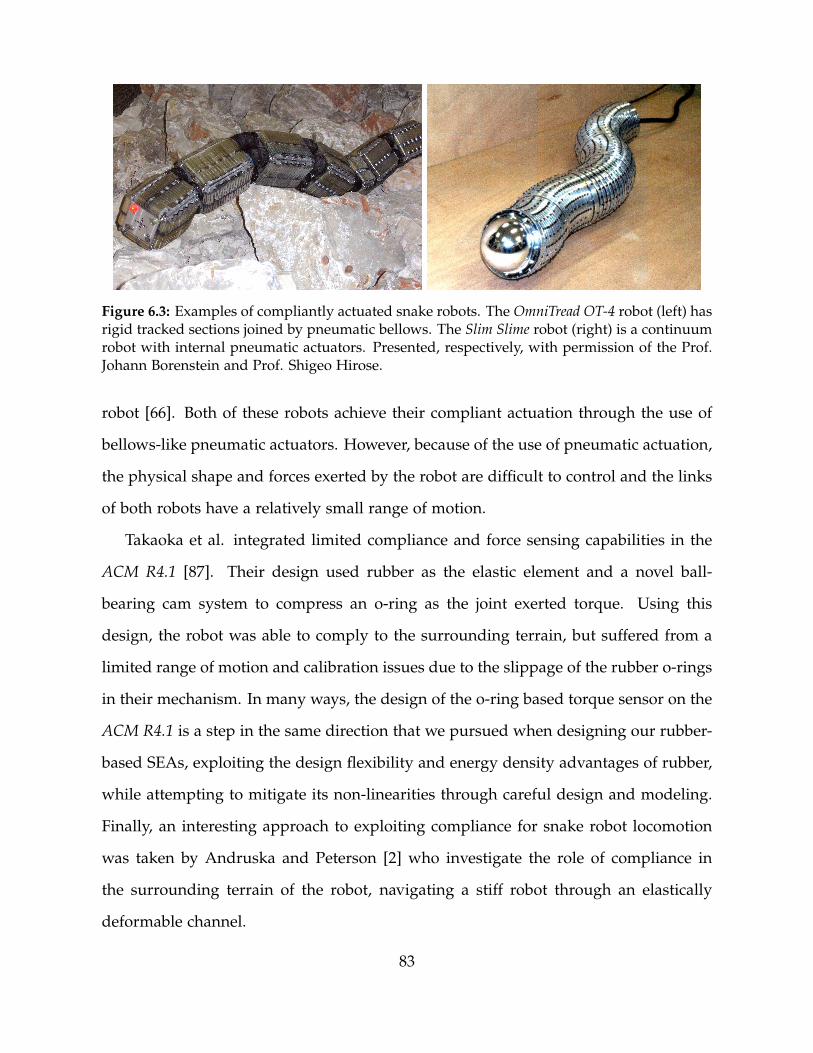
Figure 6.3: Examples of compliantly actuated snake robots. The OmniTread OT-4 robot (left) hasrigid tracked sections joined by pneumatic bellows. The Slim Slime robot (right) is a continuumrobot with internal pneumatic actuators. Presented, respectively, with permission of the Prof.Johann Borenstein and Prof. Shigeo Hirose.

robot [66]. Both of these robots achieve their compliant actuation through the use of

bellows-like pneumatic actuators. However, because of the use of pneumatic actuation,

the physical shape and forces exerted by the robot are difficult to control and the links

of both robots have a relatively small range of motion.

Takaoka et al. integrated limited compliance and force sensing capabilities in the

ACM R4.1 [87]. Their design used rubber as the elastic element and a novel ball-

bearing cam system to compress an o-ring as the joint exerted torque. Using this

design, the robot was able to comply to the surrounding terrain, but suffered from a

limited range of motion and calibration issues due to the slippage of the rubber o-rings

in their mechanism. In many ways, the design of the o-ring based torque sensor on the

ACM R4.1 is a step in the same direction that we pursued when designing our rubber-

based SEAs, exploiting the design flexibility and energy density advantages of rubber,

while attempting to mitigate its non-linearities through careful design and modeling.

Finally, an interesting approach to exploiting compliance for snake robot locomotion

was taken by Andruska and Peterson [2] who investigate the role of compliance in

the surrounding terrain of the robot, navigating a stiff robot through an elastically

deformable channel.

83

Figure 6.4: The Kulko robot from NTNU. This robot has spherical housing and force sensingresistors in each link, and performs obstacle-aided locomotion by controlling the contact forcesalong its body. Printed with permission of the authors of [57].

6.3 Torque and Force Control for Snake Robot Locomotion

Prior work with biological snakes has primarily focused on classifying and analyzing

the kinematics of their locomotion [37, 62]. More recent work has focused on measur-

ing and modeling the torques and forces involved with a snake’s interaction with the

world [21, 25, 31].

Hirose’s work with the original ACM [30] suggests a model for torque control based

on the curvature along the robot’s backbone. For a snake robot with passive wheels

(the extreme case of anisotropic friction) he theoretically proves that a snake robot can

propel itself forward merely by undulating the backbone. The work of Date [12] and

others [47], experimentally demonstrate that a torque law based on the derivative of

the robot’s backbone curvature, coupled with tactile sensing, can propel a wheeled

snake over obstacles and through corridors. Kamegawa et al. [46] further extend this

approach in simulation for a robot with torque controlled joints and tactile sensing.

A group at NTNU has focused on performing force-based obstacle aided locomo-

tion for a snake robot without wheels. Transeth et al. have presented an extensive

non-smooth model-based approach for control [91]. And more recently, Liljeback has

experimentally demonstrated obstacle aided locomotion in a lab environment for vari-

84

ous configurations of obstacles [57] with their robot Kulko, shown in Fig. 6.4. This robot

senses contact forces along its body with force sensing resistors distributed throughout

the robot, and controls these contact forces to propel itself forward.

All of the aforementioned work relies on snake robots with tactile sensing. Because

tactile sensing is difficult to robustly implement in a field robot, an alternative ap-

proach to compliant locomotion is to design controllers that adapt to the terrain solely

through control of joint torques, without explicitly sensing the robot’s contacts with

the world. The final contribution of this thesis explores different motions that follow

this approach, implemented on the SEA Snake robot. In Chapter 9 we present a variety

of low-impedance motions for snake robots. These motions demonstrate obstacle-aided

locomotion as well as other novel behaviors, based on extensions of existing work by

our group [88] and others.

85

86

Chapter 7

Design of a Compact Series Elastic

Actuator

Incorporating series elasticity into a high-performance robot is not a trivial task. Our

snake robots are similar to most other mobile robots in that they rely on highly-geared

electric motors for actuation, providing large torques at slow speeds. For example

the modules of the Unified Snake robot use a brushed DC motor and a 400:1 gear

train to produce peak torques of over 2.7 N-m and a maximum speed of 30 rpm. In

order to be used in our snake robots, the series elastic element needs to have excellent

energy storage and strength, fit in an extremely small design space, and be able to be

manufactured reliably in large quantities (our lab currently has 60 snake modules).

This work details the design, fabrication, and modeling of a high-performance se-

ries elastic element that torsionally shears rubber between two rigid plates. We show

that this design meets all of the above design criteria, and that the spring’s character-

istics can be modeled well enough to enable accurate torque sensing for field robots.

87

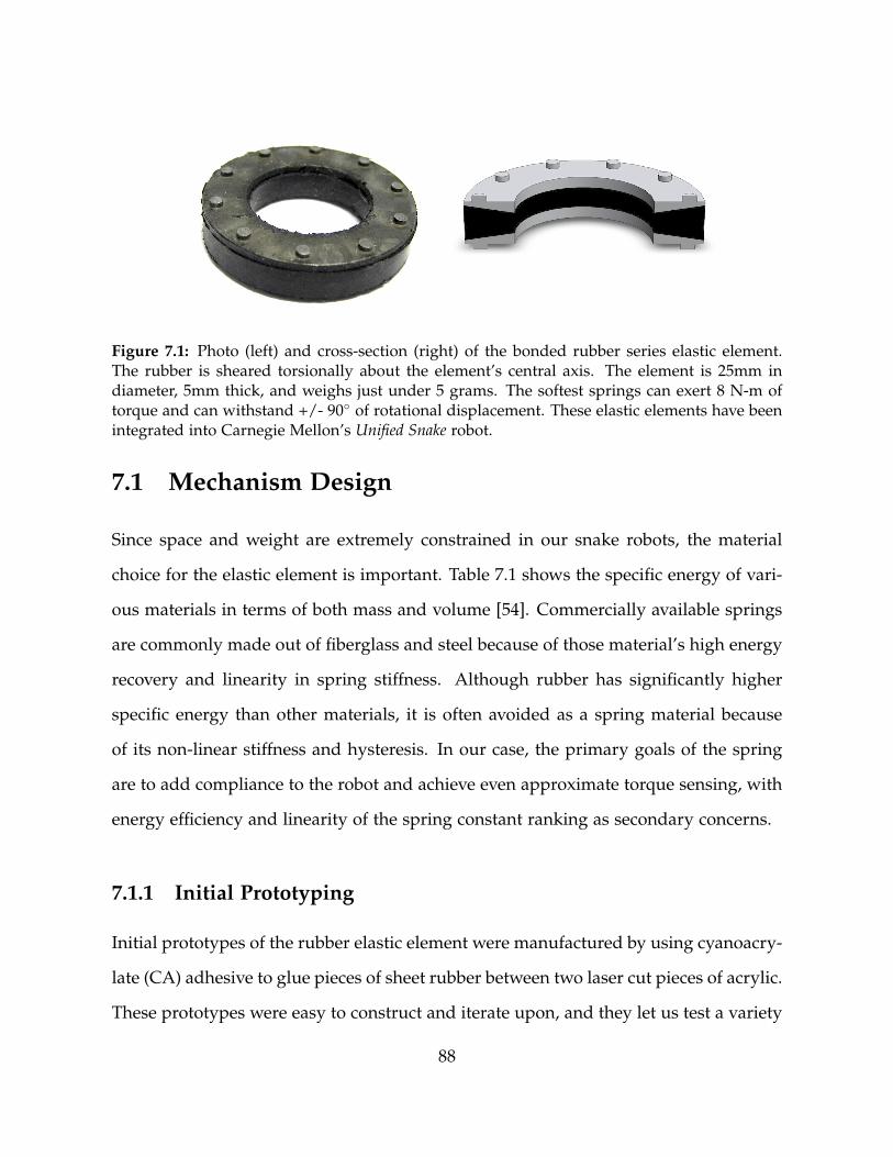
Figure 7.1: Photo (left) and cross-section (right) of the bonded rubber series elastic element.The rubber is sheared torsionally about the element’s central axis. The element is 25mm indiameter, 5mm thick, and weighs just under 5 grams. The softest springs can exert 8 N-m oftorque and can withstand +/- 90◦ of rotational displacement. These elastic elements have beenintegrated into Carnegie Mellon’s Unified Snake robot.

7.1 Mechanism Design

Since space and weight are extremely constrained in our snake robots, the material

choice for the elastic element is important. Table 7.1 shows the specific energy of vari-

ous materials in terms of both mass and volume [54]. Commercially available springs

are commonly made out of fiberglass and steel because of those material’s high energy

recovery and linearity in spring stiffness. Although rubber has significantly higher

specific energy than other materials, it is often avoided as a spring material because

of its non-linear stiffness and hysteresis. In our case, the primary goals of the spring

are to add compliance to the robot and achieve even approximate torque sensing, with

energy efficiency and linearity of the spring constant ranking as secondary concerns.

7.1.1 Initial Prototyping

Initial prototypes of the rubber elastic element were manufactured by using cyanoacry-

late (CA) adhesive to glue pieces of sheet rubber between two laser cut pieces of acrylic.

These prototypes were easy to construct and iterate upon, and they let us test a variety

88

Material Specific Energy Energy Density(mass) (volume)

Steel 140 Jkg 1 J

cm3

Fiberglass 770 Jkg 1.5 J

cm3

Rubber 5200 Jkg 5 J

cm3

Table 7.1: The specific energies and energy densities of commonly used spring materials. Byboth weight and volume, rubber has by far the greatest performance [54].

Figure 7.2: A photo of one of the early prototypes of the series elastic spring. The rubberelement is latex sheet, which is glued to acrylic plates. The spring is 38 mm (1.5 in) in diameterand 10 mm (.4 in) thick.

of different rubber types and durometers. Through this rapid iteration we found that

ultimate strengths of up to 8 N-m (6 ft-lbs) of torque and maximum deflections of up

to 90◦ were possible in a package that had an outer diameter of less than 25 mm (1

in) and a thickness of 5 mm (.19 in). Although the CA adhesive bonded particularly

on neoprene rubber, getting a consistent bond across multiple spring prototypes of

different materials proved difficult. This motivated our transition to having the next

iteration of springs molded by a professional rubber supplier.

7.1.2 Tapered Design

Initial prototypes of the spring had a flat layer of rubber between the top and bottom

plates. To maximize the ultimate load of the rubber inside the element, the cross-

89

R1

R2

dA

Hh

r

Figure 7.3: A diagram of the top view (left) and cross-section (right) of the conical taperedspring.

section of the element was later designed with a conical taper that intersects at the

center of the spring, as shown in Fig. 7.3. This taper generates uniform shear stress

across the entirety of the rubber, as opposed to a flat cross section where the periphery

of the rubber is stressed more. Since the maximum shear stress in rubber is what

limits the ultimate strength of the spring, designing the spring to uniform shear stress

maximizes its ultimate strength.

The amount by which a tapered conical spring design increases the stiffness and

strength of the spring can be calculated by integrating the spring’s internal shear forces

[20]. The torque T generated by the spring is a function of the shear stress τ integrated

over differential rings of radius r

T =∫

r τ(r) (2πr dr). (7.1)

As an approximation, we assume the shear stress is proportional to the rubber’s

shear modulus G, the spring’s rotational displacement θ, the distance from the center

of the spring r, and the thickness of the rubber h

τ(r) =Gθr

h. (7.2)

Substituting into (7.1) and integrating from the spring’s inner radius R1 to its outer

90

radius R2 yields

T = 2πGθ∫ R2

R1

r3

h(r)dr. (7.3)

For a spring with a flat cross-section, the rubber has uniform thickness, H, through-

out its radius

Tflat =πGθ

2H(R4

2 − R41). (7.4)

For the conical taper cross-section, the rubber thickness increases linearly with in-

creasing spring radius

Ttaper =2πR2Gθ

3H(R3

2 − R31). (7.5)

To calculate the amount of increase in failure torque in the tapered spring compared

to the flat spring, we take the ratio of (7.4) and (7.5) and express the result in terms of

the ratios of the inner and outer radii of the spring

ρ =R1

R2(7.6)

β =Ttaper

Tflat=

4(1− ρ3)

3(1− ρ4). (7.7)

This torque ratio β is greater than 1 for all R1 < R2. A plot of the torque ratio as

a function of the ratio of inner and outer spring radius is shown in Fig. 3. For the

springs presented in this thesis ρ = 0.6, yielding a theoretical improvement in ultimate

load and energy storage of 20% by using a tapered conical cross-section compared to

a flat cross-section.

91

0 0.2 0.4 0.6 0.8 11

1.1

1.2

1.3

1.4

ρ

To

rqu

e R

atio

β

Figure 7.4: The ratio of increased stiffness and ultimate strength of a tapered cross-sectionelastic member compared to one with a flat cross-section for a range of ratios of inner andouter radii of the spring.

7.1.3 Manufacturing and Molding

For the most recent iteration of springs, we engaged a professional rubber molding

company to mold neoprene and natural rubber to conical steel plates (Fig. 7.1). To test

the maximum compliance that can be afforded by this spring design, we chose to have

a set of springs fabricated with the softest durometer rubber available. In the initial

prototypes, we tested 3 different rubbers: 40A durometer neoprene, 40A durometer

natural rubber, and 50A durometer natural rubber.

The top and bottom plates for the spring were designed with a circular pattern

of posts that enable the springs to be integrated into the final gear stage of our snake

robot modules. The conical spring adapter plates were fabricated from cold-rolled steel

bar, using conventional turning and CNC machining processes. To enhance bonding

of the rubber, the surface of each plate was treated with a microcrystalline calcium

modified zinc phosphate coating. This treatment process was provided by Rampart

Industries in Detroit, Michigan. The molding was performed by MPS Manufacturing

in New Philadelphia, Ohio.

The rubber spring material – 40-50 durometer natural rubber or neoprene – was

compression molded at 150◦ C. The process of bonding the rubber material to the

metal was preceded by an aerosol spraying of a primer and top coat to the clean metal

92

surface. A period of 24 hours was allowed between applying the primer and molding

the parts so that chemical preparation had ample time to evaporate out of the coating

so as not to cause bond failure. The metals were then inserted into the 150◦ C mold

with approximately 4.5 g of rubber. The process of molding took 490 seconds per

spring. The assembly was then removed from the mold and the flash was removed

manually from the completed part. Finally, the part was allowed to cool slowly until it

reached room temperature. The final part weighs 5 g, with 1.8 g of rubber bonded in

between two 1.6 g steel plates.

7.2 Modeling

To load test the springs, we built a small torque-sensing test rig. Our goals for testing

were to determine the ultimate strength of various spring designs and rubber types,

to characterize the linearity of various spring designs, and to make initial attempts

to model hysteresis and other non-linear effects of the springs’ torque-displacement

curves.

Overall, the rubber springs were surprisingly linear (Fig. 7.5), with the caveat that

the spring constant softened after initial load cycling. This softening effect, known as

the Mullins effect, is a well-documented phenomenon in most rubber elastomers [48].

Linear spring constants were fit to torque displacement data for all 3 springs after they

had been initially load cycled. The best-fit spring constants and their average errors

are presented in Table 7.2.

Modeling hysteresis was attempted using a model similar to a viscoplastic material

model [48]. This physical model approximates the rubber as three parallel elements: a

linear spring, a linear damper, and a frictional element with a series spring. Each of

these elements has coefficients that are fit by optimizing the average squared error of

the predicted model torque compared the actual spring torques measured by our test

93

Neo 40A NR 40A NR 50ALinear Model Error 8.9% 9.1% 5.5%

Hysteresis Model Error 5.1% 8.6% 2.6%Spring Constant (N-m / ◦) .055 .059 .101

Table 7.2: Average error and approximate spring constants for the 3 different rubber materialsin the conical taper springs.

rig. Matlab’s fminsearch optimizer was used to fit the parameters.

There are five parameters to be identified in this model: a spring coefficient, a vis-

cous damping coefficient, a coefficient of friction of the frictional element, a yield force

of the frictional element, and a spring coefficient in series with the frictional element.

Figure 7.6 shows the predicted torque-displacement curve from this model along with

the actual torque-displacement curve for the 40A durometer neoprene spring.

7.3 Testing and Validation

The elastic elements using 50A durometer natural rubber have been integrated into

one of our lab’s Unified Snake robots (Fig. 4.1). While we are unable to measure the

deflection of the spring in the modules, we have been endurance testing them in the

everyday use of our robot. No failures due to fatigue have occurred in the 19 retro-

fitted modules in over 6 months of use. Other tests to characterize the springs have

been performed on a test jig.

7.3.1 Ultimate Strength

The molded springs that we tested to failure were 50A natural rubber, and had an

ultimate strength of approximately 8 N-m at over 60◦ of displacement. Assuming a

linear spring constant, the springs are storing approximately 6 J of energy. Since there

is only 1.8 g of rubber in the spring, the rubber is theoretically exhibiting a specific

94

energy density of approximately 3,000 J / kg, on the order of what can reasonably be

expected for rubber (Table 7.1).

Unlike previous prototypes where failures typically occurred at the bond between

the rubber and the rigid substrate, failures occurred primarily in the rubber element

itself. To calculate a rough benchmark of spring performance, we can estimate the

energy storage of the spring. The energy stored in a rotary spring with a linear spring

constant k and deflection angle θ is

E =12

kθ2. (7.8)

Fatigue tests of the spring were run by installing the springs into the final stage of

the gear train of one of our Unified Snake robot modules. By locking the output hub

of the module in place and commanding a 1 Hz sinusoidal oscillation, the spring was

subjected to repeated loading of approximately 2.6 N-m (2 ft-lbs).

The rubber in the these molded springs failed after approximately 10,000 cycles.

However, it is difficult to determine how realistic this test is compared to real world

use. In some cases, it appears that the rubber may have been heating up to the point

where it actually began to melt. Unfortunately, the deflection of the spring could not

be measured in this configuration so it is difficult to determine how much power was

being dissipated in the spring during the test.

7.3.2 Preliminary Torque Control

As an initial proof of concept, we implemented a simple torque controller, using one

of our Unified Snake robot modules and a molded 40 durometer natural rubber series

elastic element. The module and spring were attached to a test rig that measured the

output torque of the module and the absolute displacement of the spring. The torque

was measured with a load cell that was attached to a lever arm that could be pivoted by

95

hand. The robot module was commanded to exert a constant torque of 1.3 N-m, based

on the spring’s deflection and a linear spring constant, while the position of the lever

arm was varied by hand. The feedback loop on estimated torque ran at approximately

17 Hz. The results of one of these tests is shown in Fig. 7.7.

While the module did a relatively poor job of tracking the commanded force, the

estimated torque based on spring deflection was accurate to within 5%. The problems

with using motor current to estimate force are also apparent in Fig. 7.7. In particular,

stiction in the gear train causes the motor current to repeatedly drop to zero even

though the module is actually exerting a significant torque.

96

−40 −20 0 20 40−3

−2

−1

0

1

2

3

displacement (deg)

torq

ue (N

−m)

(a) Neoprene - 40A Durometer

−40 −20 0 20 40−3

−2

−1

0

1

2

3

displacement (deg)to

rque

(N−m

)

(b) Natural Rubber - 40A Durometer

−40 −20 0 20 40−3

−2

−1

0

1

2

3

displacement (deg)

torq

ue (N

−m)

(c) Natural Rubber - 50A Durometer

Figure 7.5: A comparison for torque-displacement profiles for 3 different spring materials. Theneoprene shows the most hysteresis and the lowest stiffness. The natural rubber springs havesignificantly less hysteresis. All of the the springs are approximately linear over a +/- 2.6 N-mtorque range. The springs were cycled 3 times in increasing torque from from +/- .7 N-m to+/-2.6 N-m.

97

−50 0 50−3

−2

−1

0

1

2

3

displacement (deg)

torq

ue (N

−m)

Torque−Displacement Relationship: 40A Neoprene

Actual TorqueModel Torque

Figure 7.6: The measured (blue solid line) and modeled (red dashed line) torque-displacementcurves for the 40A durometer neoprene spring, which exhibited the most hysteresis of thesprings we tested. The spring was cycled through a torque of +/-2.6 N-m (2 ft-lbs).

0 5 10 15 20 25 300

0.2

0.4

0.6

0.8

1

1.2

1.4

1.6

time (sec)

torq

ue (N

−m)

Measured TorqueSpring−Model TorqueMotor Current

Figure 7.7: The estimated and actual torque for a trial where a 40A durometer natural rubberelastic element was deflected on a test rig by one of our Unified Snake robot modules. Themodule was commanded to hold a torque while the angular position of the output hub wasmanually varied. Even though the applied force varied significantly from the commandedvalue, a simple linear model of the spring’s deflection (red dashed line) was able to accuratelypredict the measured torque (solid blue line), compared to attempts to model the torque basedon motor current (black dotted line).

98

Chapter 8

Incorporating Torque Control

With the addition of series elastic actuation to our snake robots, the need now arises to

incorporate torque control into the low-level controllers on each module. This chapter

discusses the initial implementation of hybrid position-velocity-torque control on the

modules of the SEA Snake, shown in Fig. 8.1, and presents a philosophy on controlling

SEAs that, to our knowledge, differs significantly from conventional wisdom. In par-

ticular, we discuss the benefits of using relatively low control gains and deliberately

incorporating damping in both the design and control of the actuator. This differs from

most other work with SEAs that stress efficiency and energy recovery as goals of their

control as well as attempt to make up for an SEA’s inherent lack of high-frequency

force bandwidth by running a strong force control loop on the actuator.

This chapter provides an overview of the performance characteristics of the series

elastic actuator of the SEA Snake. We should note that the SEA in this robot is of the

same overall design but slightly larger than the one presented in the previous chapter.

This allows for greater ultimate strength of 12 N-m, and slightly increased stiffness of

8 N-m / radian, to better match the torque capabilities of the SEA Snake robot. We

include basic frequency analysis of the actuator and reasoning behind our gain tuning

and architecture of the control loops.

99

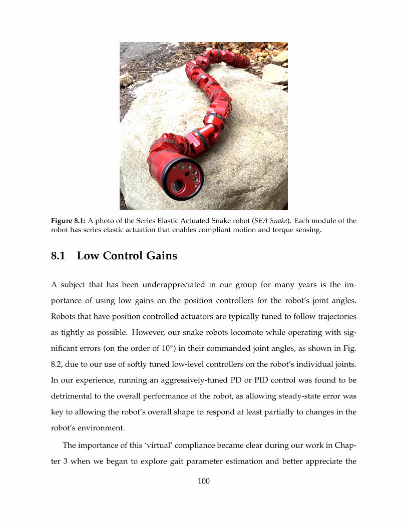
Figure 8.1: A photo of the Series Elastic Actuated Snake robot (SEA Snake). Each module of therobot has series elastic actuation that enables compliant motion and torque sensing.

8.1 Low Control Gains

A subject that has been underappreciated in our group for many years is the im-

portance of using low gains on the position controllers for the robot’s joint angles.

Robots that have position controlled actuators are typically tuned to follow trajectories

as tightly as possible. However, our snake robots locomote while operating with sig-

nificant errors (on the order of 10◦) in their commanded joint angles, as shown in Fig.

8.2, due to our use of softly tuned low-level controllers on the robot’s individual joints.

In our experience, running an aggressively-tuned PD or PID control was found to be

detrimental to the overall performance of the robot, as allowing steady-state error was

key to allowing the robot’s overall shape to respond at least partially to changes in the

robot’s environment.

The importance of this ‘virtual’ compliance became clear during our work in Chap-

ter 3 when we began to explore gait parameter estimation and better appreciate the

100

667 668 669 670 671 672 673 674 675 676 677

−0.4

−0.3

−0.2

−0.1

0

0.1

0.2

0.3

0.4

Angles − Module 7

time (s)

angle

(ra

d)

Figure 8.2: Example of commanded and feedback joint angles from one of the modules duringpipe crawling. Note that the actual joint angles (solid line) significantly lag the commandedangles (dashed line) due to the modules low proportional gain.

locomotion of the robot with respect to its overall shape changes. Angular errors in

the robot’s commanded joint angles that would normally be considered large have a

relatively small effect on the robot’s overall shape. Furthermore, these individual er-

rors are what allowed the robot to handle significant bends in its geometry with no

high-level adjustments to its shape. For example, the Unified Snake robot was able to

negotiate 90◦ bends on the outsides of pipes with only commanding the nominal gait

designed for locomoting on straight poles. The joint angle errors allowed by low con-

trol gains, spread across all the modules in the snake robot, were a key component in

allowing the robot to adapt its shape to changes in its environment with unmodified

feedforward joint trajectories. However, we should point out that the robot’s actuation

limited its compliant characteristics to pipes and channels, where the robot could exert

many times its own body weight. To comply to irregular terrain on the ground, passive

compliance and torque control is needed.

This simple proportional controller with a relatively soft gain on each module has

been used without change on our robots, until the recent addition of series elasticity

as a retrofitted modification to one the Unified Snake robots [80]. In the robot that was

101

retrofitted with series elasticity, a derivative term was added to damp out oscillations

from the spring, but the proportional gain was left unmodified.

With SEAs, it is common to design the springs to be as linear as possible and run a

relatively high-gain controller on spring deflection so that the actuator can approximate

a perfect torque source within its control bandwidth. Our experience with using low

gains for the joint angle position controllers on our snakes led us to make two unique

choices in the design and control of the SEA Snake; to accept significant amounts of

non-linearity and inaccuracy in torque sensing and to continue to rely on relatively

low-gain controller tuning, this time on the inner torque control loop running on the

SEA.

First, we are willing to sacrifice linearity of the springs, and thus absolute accuracy

of torque sensing, in order to gain the strength and energy density benefits of using

rubber as the spring material. When locomoting with our stiffly actuated snake robots,

the joint angles typically deviate from their commanded values by as much as 10-20%.

We hypothesize, and demonstrate in Chapter 9, that a similar level of accuracy in

torque sensing is still enough to enable useful low-impedance locomotion.

Second, we run a relatively low-gain torque control loop, rather than the high-gain

torque control that is typically done with SEAs [33, 73]. Given that our rubber SEAs

are less accurate than traditional SEAs, this may come as no surprise. However, run-

ning a high-gain torque control loop on an SEA makes some sense from a theoretical

standpoint. The closer the actuator is to a perfect torque source, the easier it is to

analyze and perform precise motion control. Additionally, a high-gain controller will

also increase the bandwidth of the actuator beyond the passive dynamics of the motor

inertia and spring. In [73], Robinson shows that the controlled stiffness of the actuator,

kc, is increased by

kc = ks(1 + Kp), (8.1)

102

where ks is the stiffness of the spring in the SEA and Kp is the proportional control

gain of the torque controller. This controlled stiffness, along with the load and motor

inertias, determine the natural frequency and the control the bandwidth of the actuator.

However, driving an actuator near or past its resonant frequency is commonly

known to be difficult [86]. Overall, we feel the stability issues caused by high control

gains interacting with the actuator’s stiction and backlash are a significant problem that

is often overlooked in the design and control of SEAs. Additionally, mobile robots are

always pushing their performance envelope, and spend a significant amount of time

near saturation. For these reasons, relying on the motor to extend an SEA’s bandwidth

is perhaps an overly optimistic goal.

8.2 Damping

A common motivation for using SEAs is the ability to store energy from the robot’s

motions, making them theoretically attractive for dynamic walking and running robots.

With snake robots, our goals for using SEAs are primarily for torque control and shock

protection, with energy storage and recovery being less important. Furthermore, we

note that both Robinson [73] and Hurst [33] comment in their respective PhD theses the

need to incorporate more controller damping in practice than theoretically expected.

This has led us to embrace the inherent damping in the design of the actuators, and

realize the importance of incorporating it for control.

The choice to use rubber springs in our SEAs means that the actuators are inherently

damped, as seen by the hysteresis in Fig. 7.5. Attempts to accurately characterize this

damping have proved to be difficult, as it seems to be a combination of visco-elastic and

elasto-plastic effects. While this makes traditional analysis and accurate simulation of

the SEA more difficult, energy is being removed from the system and will likely have

a stabilizing effect.

103

Fm Im

bs

ksbm

Fl

June 11, 2014DRAFT

100

101

0.1

0.5

1

Forc

e R

atio

Frequency (Hz)

100

101

−270

−180

−90

0

Phase

(deg)

Frequency (Hz)

4 N−m2 N−m1 N−m

4 N−m2 N−m1 N−m

Figure 8.6: A Bode plot showing the bandwidth of the series elastic actuator at different am-plitudes of oscillation. We have chosen to tune the in torque control loop so that it is close tocritically damped.

cl = 2p

kc Il. (8.5)

Equation (8.4) assumes that the output is fixed, or in other words has infinite inertia.

Qualitatively, if the output has some smaller inertia and can accelerate, the effective

spring constant is reduced and setting the damping gain to (8.4) will over damp the

actuator. Similarly, (8.5) assumes a fixed motor (not necessarily an accurate assump-

tion).

Since the load inertia, Il, changes during locomotion it helps to qualitatively con-

sider the effects of Il being larger or smaller than the geared motor inertia, h2 Im. If Il

< h2 Im, the resonant frequency is higher and the critical damping coefficient is lower,

and to be conservative we are better off setting the gain so that the motor’s oscillations

remain critically damped. If Il > h2 Im then the resonant frequency is lower and the

106

Figure 8.3: Model of the SEA with a fixed output for torque bandwidth testing. The motordamping parameter, cm (in blue), was determined empirically from measured data, while theremaining parameters (in black) were set based on the identified motor and spring parameters.

SEA Model ParametersParameter Value Units

ks 8 N-m / radbs 0.02 N-m / (rad/s)η 349 : 1Im 5.1× 10−7 kg-m2

bm 0.5 N-m / (rad/s)

Table 8.1: Parameters of the SEA used for modeling.

To test the torque bandwidth of a SEA Snake module, we clamped the output and

commanded sinusoidal oscillations of increasing frequency, as shown in Fig. 8.3. In

addition to measuring the response of the real actuator, a model based on the same pa-

rameters of the SEA, including motor saturation, was simulated. The damping of the

rubber spring was simplified and modeled as viscous friction. The identified parame-

ters of the spring and motor are provided in Table 8.1, and with the exception of motor

damping, bm, are based on either previous calibration of the spring, or specifications

of the motor, a Maxon EC-Flat 20 brushless DC motor.

The first set of tests were performed with a high gain on the torque controller,

Kp = 25, and no damping, Kd = 0. In theory, with the output of the actuator fixed, the

torque bandwidth should drop off past the controlled natural frequency of the motor,

104

100

101

.1

.5

1.01.5

Fo

rce

Ra

tio

Frequency (Hz)

100

101

−270

−180

−90

0

Ph

ase

(d

eg

)

Frequency (Hz)

Simulated

Measured

Simulated

Measured

Figure 8.4: A Bode plot showing the bandwidth of the series elastic actuator of the SEA Snake.The amplitude of oscillation was 1 N-m. Simulated parameters were based on motor data andidentified spring parameters, with the motor damping tuned to match the measured data.

ωm =

√kc

η2 Im. (8.2)

For the modeled system with no motor saturation (8.2), we would expect the actuator

bandwidth to be extended out to the controlled natural frequency of 7.5 Hz. This is

significantly beyond the 2 Hz natural frequency of the passive system, where kc = ks.

In Figs. 8.4 and 8.5, the dashed blue line is the response of a simulated system

using the parameters of the motor and spring in the SEA Snake. The upper plot shows

the ratio of commanded input force to actual output force as fraction on a log scale

as opposed to dB attenuation on a linear scale. Figure 8.4 shows the response of the

SEA to sinusoidal oscillations of 1 N-m. Without any damping in the torque controller,

there is a slight peak before motor saturation starts to dominate. The bandwidth of the

actuator starts to roll off at 5 Hz, showing the effect of the controller gain. However,

105

100

101

0.1

0.5

1

Fo

rce

Ra

tio

Frequency (Hz)

100

101

−270

−180

−90

0

Ph

ase

(d

eg

)

Frequency (Hz)

Simulated

Measured

Simulated

Measured

Figure 8.5: A Bode plot showing the bandwidth of the series elastic actuator of the SEA Snake.The amplitude of oscillation was 5 N-m. Simulated parameters were based on motor data andidentified spring parameters, with the motor damping tuned to match the measured data.

motor saturation is also apparent as the bandwidth does not extend out the 7.5 Hz that

would be predicted with no motor limitations.

The Bode plot in Fig. 8.5 even more clearly shows the effect of motor torque satura-

tion, qualitatively damping the system at large amplitudes. As the motor reaches the

limits of its capabilities the natural dynamics of the system dominate, and bandwidth

decreases past the passive natural frequency of 2 Hz. As indicated in the Table 8.1, the

motor damping coefficient, bm, was found to be quite significant, 0.5 N-m / (rad/sec).

It is interesting to note that if bm is set to zero, the model is numerically unstable,

further indicating how important damping is to the stability of the control of SEAs.

106

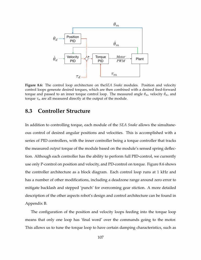
Position PID

Velocity PID

Torque PID

Motor PWM

+

✓d

✓d

⌧d⌧m

✓m

✓m

Plant

Figure 8.6: The control loop architecture on theSEA Snake modules. Position and velocitycontrol loops generate desired torques, which are then combined with a desired feed-forwardtorque and passed to an inner torque control loop. The measured angle θm, velocity θm, andtorque τm are all measured directly at the output of the module.

8.3 Controller Structure

In addition to controlling torque, each module of the SEA Snake allows the simultane-

ous control of desired angular positions and velocities. This is accomplished with a

series of PID controllers, with the inner controller being a torque controller that tracks

the measured output torque of the module based on the module’s sensed spring deflec-

tion. Although each controller has the ability to perform full PID-control, we currently

use only P-control on position and velocity, and PD-control on torque. Figure 8.6 shows

the controller architecture as a block diagram. Each control loop runs at 1 kHz and

has a number of other modifications, including a deadzone range around zero error to

mitigate backlash and stepped ‘punch’ for overcoming gear stiction. A more detailed

description of the other aspects robot’s design and control architecture can be found in

Appendix B.

The configuration of the position and velocity loops feeding into the torque loop

means that only one loop has ‘final word’ over the commands going to the motor.

This allows us to tune the torque loop to have certain damping characteristics, such as

107

critically damping the internal oscillations of the spring and motor.

This is set of cascaded controls was chosen over 2 alternatives. The first alterna-

tive is where the position, velocity and torque control loops are cascaded in series,

with a position error feeding to a velocity controller, and velocity error feeding into a

torque controller. This was avoided because the velocity measurements on the module

are very noisy. The second alternative is a flat architecture, where torque, velocity,

and position controllers are all summed together into a single motor signal. This con-

figuration may prove useful in the future, as it allows more predictable behavior of

the velocity and position controllers by bypassing the torque controller. However, our

current configuration in Fig. 8.6 has the benefit that it is more intuitive to tune out

oscillations of the SEA since only one loop has final control over the commands to the

motor, and the position and velocity loops have gains in the intuitive units of error per

N-m of torque.

8.4 Gain Tuning

When tuning the frequency response of an SEA, there are two natural frequencies that

need to be considered; the frequency of internal oscillation, ωm, of the spring and the

geared motor (8.2), and the frequency of external oscillation, ωl, of the spring and the

actuator load,

ωl =

√kc

Il. (8.3)

We note that the internal natural frequency of the motor and spring, ωm, is static

and depends only on the controlled stiffness kc from (8.1) and the motor inertia, Im,

seen through gear ratio, η. In contrast, the natural frequency of the output of the

actuator, ωl, varies over time, since inertia of the actuator load, Il, varies continuously

108

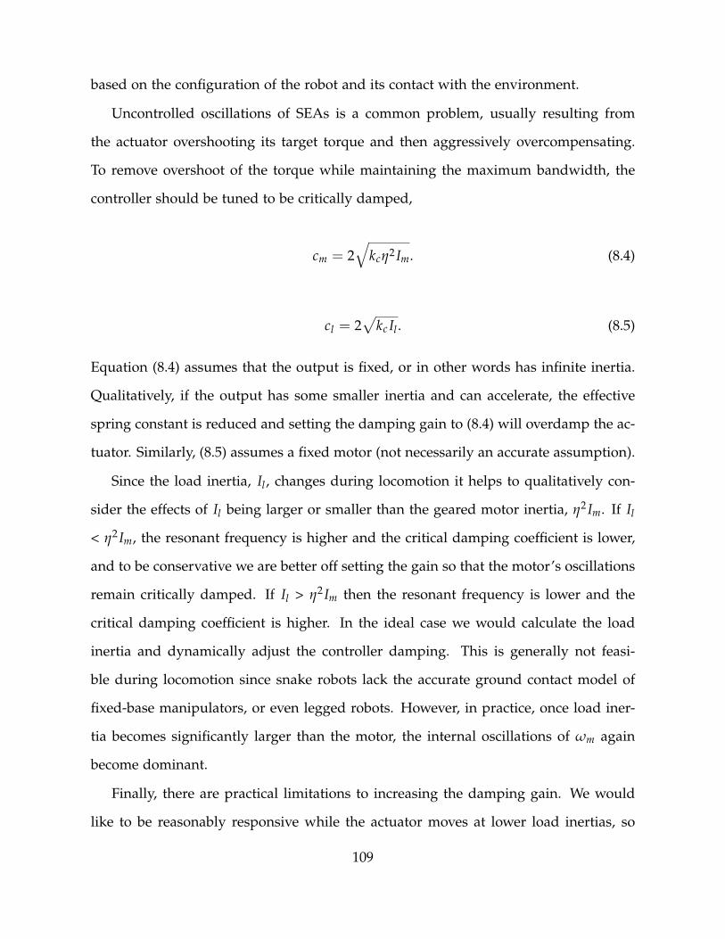
based on the configuration of the robot and its contact with the environment.

Uncontrolled oscillations of SEAs is a common problem, usually resulting from

the actuator overshooting its target torque and then aggressively overcompensating.

To remove overshoot of the torque while maintaining the maximum bandwidth, the

controller should be tuned to be critically damped,

cm = 2√

kcη2 Im. (8.4)

cl = 2√

kc Il. (8.5)

Equation (8.4) assumes that the output is fixed, or in other words has infinite inertia.

Qualitatively, if the output has some smaller inertia and can accelerate, the effective

spring constant is reduced and setting the damping gain to (8.4) will overdamp the ac-

tuator. Similarly, (8.5) assumes a fixed motor (not necessarily an accurate assumption).

Since the load inertia, Il, changes during locomotion it helps to qualitatively con-

sider the effects of Il being larger or smaller than the geared motor inertia, η2 Im. If Il

< η2 Im, the resonant frequency is higher and the critical damping coefficient is lower,

and to be conservative we are better off setting the gain so that the motor’s oscillations

remain critically damped. If Il > η2 Im then the resonant frequency is lower and the

critical damping coefficient is higher. In the ideal case we would calculate the load

inertia and dynamically adjust the controller damping. This is generally not feasi-

ble during locomotion since snake robots lack the accurate ground contact model of

fixed-base manipulators, or even legged robots. However, in practice, once load iner-

tia becomes significantly larger than the motor, the internal oscillations of ωm again

become dominant.

Finally, there are practical limitations to increasing the damping gain. We would

like to be reasonably responsive while the actuator moves at lower load inertias, so

109

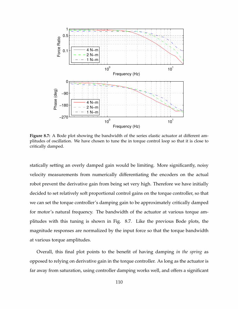
100

101

0.1

0.5

1

Fo

rce

Ra

tio

Frequency (Hz)

100

101

−270

−180

−90

0

Ph

ase

(d

eg

)

Frequency (Hz)

4 N−m

2 N−m

1 N−m

4 N−m

2 N−m

1 N−m

Figure 8.7: A Bode plot showing the bandwidth of the series elastic actuator at different am-plitudes of oscillation. We have chosen to tune the in torque control loop so that it is close tocritically damped.

statically setting an overly damped gain would be limiting. More significantly, noisy

velocity measurements from numerically differentiating the encoders on the actual

robot prevent the derivative gain from being set very high. Therefore we have initially

decided to set relatively soft proportional control gains on the torque controller, so that

we can set the torque controller’s damping gain to be approximately critically damped

for motor’s natural frequency. The bandwidth of the actuator at various torque am-

plitudes with this tuning is shown in Fig. 8.7. Like the previous Bode plots, the

magnitude responses are normalized by the input force so that the torque bandwidth

at various torque amplitudes.

Overall, this final plot points to the benefit of having damping in the spring as

opposed to relying on derivative gain in the torque controller. As long as the actuator is

far away from saturation, using controller damping works well, and offers a significant

110

amount of flexibility in tuning the frequency response of the system. However, as the

motor nears saturation the passive dynamics of the spring dominate. In our case we are

fortunate that the torque control is well-damped by the internal friction of the motor

and geartrain, but the output load is free to vibrate since the springs we initially chose

are only lightly damped. However, if the spring itself provides damping, oscillations

of both the internal motor and the external load can be mitigated regardless of actuator

saturation.

111

112

Chapter 9

Low Impedance Motions for Snake

Robots

The previous two chapters presented the design of a compact series elastic actuator

and the hybrid position/force control framework that we use for low-level motion con-

trol. This chapter takes the first step towards creating mid-level controllers that exploit

these new capabilities, and presents the preliminary results of using the compliant ac-

tuation of the SEA Snake to perform low impedance locomotion. By low impedance,

we mean motions where changes in the robot’s shape are primarily driven by its inter-

action with the environment and robot’s commanded joint torques, rather than being

driven directly by the robot’s commanded joint angles. These motions have the advan-

tage that they passively comply to the surrounding terrain, without adding additional

complexity to the controller and without needing tactile sensors on the robot.

Despite the preliminary nature of this work, we feel it is significant for three rea-

sons. The first is that we demonstrate that simple methods of controlling the torques

of the SEA Snake robot’s joints provides compliant locomotion significantly beyond

what complex methods were able to accomplish with the stiffly actuated Unified Snake.

The second is that we demonstrate, through the use of our approximately calibrated

113

rubber-based SEAs, that precise and accurate torque control is not needed to accom-

plish at least some types of snake locomotion. The spring constants of the rubber

springs presented in this thesis have been able to be calibrated to within about 20%

of their actual value. Finally, to the best of our knowledge, these results are the first

demonstration of successful low-impedance and obstacle-aided locomotion of a real

robot without external force or tactile sensing.

9.1 Compliant Roll-In-Shape

The ability of our robots to twist continuously within a given backbone shape is a

property of the the torsion-free configuration of their joints, described previously in

Section 2.3.2 of this thesis and in more detail in [27]. For position controlled shapes

this can be exploited to create gaits where the backbone shape of the robot remains

constant and the robot rolls within this shape to locomote.

Yamada and Hirose discuss this configuration in detail in [105]. They refer to the

torsion-free configuration of a snake robot’s joints and the corresponding convention

of lateral and dorsal curvatures to describe the robot’s shape as a bellows model. In

particular, they note the relationship between the lateral and dorsal curvatures of the

robot κx and κy and the Frenet-Serret curvature κ to be

κ2 = κ2x + κ2

y. (9.1)

For a given curvature, κ, in (9.1), there is a continuum of values for κx and κy that

allow the robot to be twisted into different configurations around the backbone. This

extra degree of freedom can be parameterized as the clocking angle, φ, of one of the

robot’s modules around the backbone,

114

x

y

x

y

⌧

⌧x

⌧y

Figure 9.1: A visual representation of the roll-in-shape controller. The commanded torque τ iscommanded based on the local curvature κ. The commanded torque of the joint is the x or ycomponent of total torque, depending on how the joint is oriented in the robot.

φ = tan−1 κy

κx. (9.2)

By specifying φ of any one of modules defines the clocking of the curvature vector

around all the remaining modules in the robot, and by gradually adjusting φ over time

the robot can be made to twist rigidly around a given backbone shape by commanding

joint angles based on the robot’s local curvature. This property is exploited with the

rolling motions of our snake robots, particularly the gaits designed for traversing pipes

in Chapters 3 and 5.

9.1.1 Controller

If we instead use this same intuition about the robot’s backbone curvatures to com-

mand joint torques instead of joint angles, we can achieve a low-impedance version

of rolling in shape. This motion has the property that the robot still twists around its

backbone, but the backbone shape itself results from the robot’s joint torques and its

interaction with the world.

115

Intuitively, equation (9.1) represents how the total local curvature of the robot is

expressed in terms of its local lateral and dorsal curvatures. Torques can also be ex-

pressed in terms of the same vectors, and can also be broken down into its constituent

lateral and dorsal torques. If we want to increase or decrease the curvature, the ideal

torque to command would be aligned with the curvature. However, if we want to

rotate the curvature around the backbone, while changing the curvature as little as

possible, the ideal torque command would be orthogonal to the curvature, as visually

illustrated in Fig. 9.1.

As a control law on the x− and y−axis actuators on the snake robot , commanding

torques that are proportional and orthogonal to the local curvature simplifies down to a

controller where a torque about the x axis at some point along the robot is proportional

to the local curvature about the y axis, and vice versa,

τx(s) = −νκy(s)

τy(s) = νκx(s).(9.3)

In (9.3), s is the position along the robot’s backbone, and ν is a scaling parameter that

linearly maps curvature to torque. The sign of ν can be used to control whether the

robot twists clockwise or counterclockwise around its backbone shape.

If the robot’s joints are evenly spaced along the backbone, this controller can be

equivalently written in terms of joint angles of hypothetical robot with 2 DOF joints.

In this case, the parameter ν now scales between joint angles and torques,

τx(s) = −νθy(s)

τy(s) = νθx(s).(9.4)

On our snake robots, joints are alternately oriented in the lateral and dorsal planes

of the robot, as illustrated in Fig. 2.6. Because of this, at a given joint we have either

a measured θx or θy, but not both. Since the control law (9.5) requires knowledge

116

Figure 9.2: A montage of the robot undergoing the compliant roll-in-shape motion. The robotactively rolls along while compliantly adapting its shape to match its surroundings.

0 5 10 15 20 25 30−2

−1

0

1

2

time (sec)

torq

ue

(N

m)

an

gle

(ra

d)

Measured Angle

Commanded Torque

0 5 10 15 20 25 30−2

−1

0

1

2

time (sec)

torq

ue

(N

m)

Commanded Torque

Measured Torque

0 5 10 15 20 25 30−4

−2

0

2

4

time (sec)

ve

locity (

rad

/s)

Commanded Velocity

Measured Velocity

Figure 9.3: Commanded and feedback data from one of the robot’s modules for a trial ofcompliant roll-in-shape. The top plot shows the relationship of the commanded torque to themeasured joint angle. The middle plot shows the commanded vs. measured torque output ofthe module. The bottom plot shows the module’s commanded and measured velocity.

117

of the joint angle orthogonal to the joint that is being torque-controlled, we linearly

interpolate the angle based on the angles of adjacent joints s+ and s−,

θx(s) =θx(s−) + θx(s+)

2

θy(s) =θy(s−) + θy(s+)

2.

(9.5)

This interpolation also has the effect of slightly smoothing out the robot’s measured

curvature.

9.1.2 Implementation

To demonstrate the compliant roll-in-shape motion, the robot was driven over various

terrains, including people’s limbs and bodies. To improve the performance of the robot

during rolling, two modifications were made to the control law (9.5). The first is that

the velocities of the joints were damped by commanding a 0 velocity and setting a small

proportional gain on the velocity controller on each module. This simulated viscous

damping prevents the modules from rolling too quickly when there is little to resist

the robot’s motion. The second is that the commanded torques were tapered slightly

(reduced by 1/3) at the head and tail. This mitigates kinking at the head and tail of

the robot, particularly when rolling on flat ground.

A montage of the robot executing compliant roll-in-shape is shown in Fig. 9.2. The

robot easily conforms to the arms and shoulders while rolling under its own power.

Figure 9.3 shows the commanded and feedback controls from the 8th module, located

in the middle of the robot. The top figure shows the orthogonal relation between the

commanded torque and the robot’s joint angle, as well as the slight smoothing effect

from interpolating joint angles for the controller. The middle plot shows the module’s

tracking of commanded torque, where the effect of the viscous damping due to a

commanded zero velocity can be observed.

118

Figure 9.4: A visual representation of low-impedance sliding. Torques are commanded basedon the derivative of the robot’s curvature along the backbone. This has the effect of propagatingcurves in the robot along the backbone, compliantly sliding around obstacles.

9.2 Low-Impedance Sliding

Biological snakes slide through their environment smoothly pushing off of obstacles.

Snake robots have typically achieved similar motions through the use of follow-the-

leader joint angle control schemes and often using passive wheels to create an ideal

contact with the world [30]. However, when the robot needs to negotiate around obsta-

cles or through corridors, these methods can perform poorly. To address these issues,

we would like to develop a low-impedance motion that mimics biological snakes and

uses obstacles aid in locomotion rather than avoid them altogether.

9.2.1 Controller

Date and Takita [12], as well as unpublished work by Jentoft and Pratt, propose using

a control law based on the derivatives of local curvatures along the backbone of the

snake,

τx(s) = λd(κx(s))

ds

τy(s) = λd(κy(s))

ds.

(9.6)

In (9.6), λ is a scaling parameter that maps curvature to torque. This control law will

tend to amplify the trends in curvature in a direction along the snake’s backbone. The

119

direction of propagation depends on the sign of λ. Intuitively, the commanded torques

will be largest at inflection points in the curvature of the snake, as shown in Fig. 9.4.

As with the roll-in-shape controller, we can equivalently express the desired torques

with respect to the robot’s joint angles instead of curvatures,

θ′x(s) =

d(θx(s))ds

θ′y(s) =

d(θy(s))ds

.(9.7)

τx(s) = λθ′x(s)

τy(s) = λθ′y(s).

(9.8)

This controller was implemented on the robot, and during its use we observed that

modules have a tendency to kink at 90◦ and poorly propagate curvatures tail wards at

small angles. To address these issues we modified the control law from (9.8) so that

the torques were proportional to the square-root of joint angles,

τx(s) = λ sign(θ′x(s))

√|θ′x(s)|

τy(s) = λ sign(θ′y(s))

√|θ′y(s)|

(9.9)

The sign() function above returns 1 or −1, depending on whether its arguments are

positive or negative, respectively. This is needed to properly handle square-roots for

negative values of τx(s) and τy(s).

9.2.2 Implementation

To demonstrate low-impedance sliding, the robot progressed through a set of rounded

obstacles in a corridor. As with the roll-in-shape controller, the velocities of the joints

were damped, and commanded torques were tapered slightly towards the head and

tail. To decrease the coefficient of friction and smooth out the robot’s shape, we covered

120

Figure 9.5: A montage of the low-impedance sliding motion. The robot’s head oscillates untilthe shape of the robot closely matches the shapes of the buckets and the snake slides through.Afterwards, the head continues to oscillate, causing the robot to turn in place.

the body with nylon cable braid.

In order to initiate curvature to propagate down the backbone, the torque of first

joint was oscillated with a fixed frequency

τhead = A sin(ωt). (9.10)

It should be noted that this blind oscillation is an extremely naive way of setting prop-

agating the sliding motion. In the future we intend to allow an operator or higher-level

planner to actively steer the head, providing a guide for how the curvature should be

shaped. Even with this simple implementation of the controller, the robot was able to

successful negotiate the obstacles in a surprisingly life-like manner, as shown in Fig.

9.5.

9.3 Empirical Gait Construction

It could be argued that the reason snake robots move across the ground when executing

a gait is less of a result of its shape changes and more of a result of its torques that are

applied to cause those shape changes. Since position-controlled gaits are cyclic, when

designing them we tend to exploit geometric regularity of the terrain, like flat ground

and cylindrical pipes. However with torque-controlled gaits it may be possible that a

121

similar force-based regularity exists that can be exploited for gait design.

Our group, as well as others, have developed a wide range of position-controlled

gaits and motions [66, 88] that are useful in the field. While we have had some success

in making these gaits adapt to the robot’s environment [78], in general the tuning and

control of various gaits for a wide range environments is difficult. Therefore, we are

interested in methods that could endow our existing library of motions with the low-

impedance characteristics that might be enabled by torque control, without starting

gait development over from scratch.

9.3.1 Controller

To generate low-impedance versions of our existing gaits, we can execute a normal

position-controlled gait on the SEA Snake and record the robot’s feedback, including

joint angles, velocities, and torques. By executing the gait on the nominal terrain for

which the gait was designed (e.g. level ground), we hope to find cyclic velocities and

torques that correspond to ‘nominal’ locomotion. By playing back these positions,

velocities, and torques as reference trajectories, and closing the loop primarily on the

torques and velocities, we can generate a gait that closely mimics the original position-

controlled gait on the original terrain, while at the same time is more compliant to

variations and obstacles.

9.3.2 Implementation

We demonstrated the empirical construction of low-impedance gaits with the slithering

gait [88]. This motion is designed for flat ground, and is a modified version of sinus-

lifting [66] where the motion gradually tapers at the head of the robot so that the

camera image remains steady during locomotion.

The gait was executed on the SEA Snake and the feedback from each of the robot’s

122

modules was recorded at 100 Hz. Before using the feedback as a reference trajectory,

the torque and velocity trajectories for each module were smoothed with a forward-

back rolling window filter (Matlab’s smooth() function) to remove high-frequency

noise without introducing lag into the trajectory. The gains on the module controllers

were set such that the position gains were much lower compared to the velocity and

torque gains.

During the execution of the low-impedance version of slithering, the robot was able

to navigate an abrupt bend using only the nominal feedforward motion designed for

going straight, as shown in Fig. 9.6. Instead of generating large torques to maintain

a commanded shape, and instead commanding the robot’s joints to primarily track

trajectories of torques and velocities enabled the robot to accept the deformations,

negotiate the bend, and gradually return to its reference trajectory afterwards.

123

Figure 9.6: A montage of the robot undergoing the a low-impedance slithering gait. The robotexecutes the gait cycle and progress forward, but can be easily deformed form the nominalshape. This allows the robot to progress around a bend that would not have been possible witha standard position-controlled gait.

0 5 10 15 20 25 30−1.5

−1

−0.5

0

0.5

1

1.5

time (sec)

an

gle

(ra

d)

Commanded Angle

Measured Angle

0 5 10 15 20 25 30−4

−2

0

2

4

time (sec)

velo

city (

rad/s

)

Commanded Velocity

Measured Velocity

0 5 10 15 20 25 30−3

−2

−1

0

1

2

3

time (sec)

torq

ue (

Nm

)

Commanded Torque

Measured Torque

Figure 9.7: Commanded and feedback data from one of the robot’s modules for a trial of low-impedance slithering. The module primarily tracks the commanded torque and velocity. Thisallows the joint angle to deviate significantly from its commanded value without introducinglarge torques or corrections.

124

Part III

Conclusions and Future Work

125

Chapter 10

Conclusions

The work in this thesis strives to develop methods that improve the locomotion ca-

pabilities of snake robots in real-world field environments. Although the individual

contributions of this thesis span the domains of motion control, state estimation, and

actuator design, together they share the philosophy that stability and robustness is often

more important than accuracy and precision. In order to compensate for the limita-

tions of poor sensing and modeling, carefully combining different sensing modalities can

mitigate the weaknesses of individual sensors and other components. Additionally,

at all stages we seek to exploit intuition about the system and focus on simplicity in

controlling and modeling the robot as much as possible.

In the case of gait-based compliant control, this perspective leads us to build on the

existing strengths of low-dimensional parameterized gaits and the intuitive connection

between individual gait parameters and high-level behaviors. For state estimation, we

exploit the extreme redundancy in our robot’s sensors rather than intricately model the

robot’s interaction with the world. In the development of both, we follow a Kalman

filtering framework, in part because of its widespread use in the robotics community

and in part because of its natural ability to accommodate the noisy and incomplete

feedback data from our snake robots.

127

In our pursuit of intuitive tools for snake robots, we also formalize the notion of an

averaged body frame that we call the virtual chassis, and apply it to state estimation

of the robot’s shape and orientation. Compared to our preliminary work that used

simpler process models [75], the results from this thesis estimating for a wider variety

of models and gaits show that the benefits of using the virtual chassis body frame over

a fixed frame were less pronounced. While the virtual chassis remains an important

tool for intuitively understanding and developing motions for snake robots, when us-

ing higher fidelity models and increased update rates for sensing, the specific choice

of body frame becomes relatively less important.

Years of work developing and controlling the Unified Snake convinced us of the fun-

damental need to provide passive compliance and sensitive torque control in our next

snake robot. Furthermore, our experience from previous generations of snake robots

led us to a philosophy that values stability and robustness over accuracy and precision

and drove the novel design and implementation of the compact series elastic actuator

in the SEA Snake. Even though the rubber-based actuator developed in this thesis falls

short of the precision, accuracy, and energy recovery found in other SEAs, we believe

that these tradeoffs are warranted in exchange for significantly greater energy density

and strength. Furthermore, we believe that for robots where the surrounding environ-

ment, and indeed the robot itself, is poorly modeled, inherent damping in the actuator

should be embraced and exploited, rather than avoided.

While we did not originally consider this thesis to be heavily bio-inspired, in hind-

sight there is a distinct biological influence. The tools of traditional robotics, usually

developed in simulation or in a carefully managed industrial environment, are often

an inappropriate match for the unstructured but high-performance demands of artic-

ulated locomotion. The overall focus by researchers and engineers on improving the

precision and accuracy of sensors and actuators has gradually increased the capabili-

ties of many classes of robots, but advances in the locomotion of fieldable articulated

128

mobile robots, including snake robots, remains limited. For snake robots, we feel that

a lack of more accurate sensing or more powerful actuation is not the primary lim-

itation. Even the cheapest robots today contain more accurate encoders and inertial

sensors than their biological equivalents, and yet snake robots fall far short in their

capabilities. However, biological snakes have a wealth of other complementary tools

at their disposal that our robots currently lack: tactile sensing, stereo vision, hearing,

smell and taste, and specialized physical adaptations.

We believe that significant gains can be made to the practical capabilities of field

robots by taking a step back and considering the entire system more holistically. This

thesis demonstrates that the quality of a robot’s individual sensors and the fidelity of

its modelling and control are not necessarily the key to advancing its capabilities in

the field. Rather, we show the benefits of implementing a broadly capable set of sens-

ing and actuation modalities, however crude, and carefully incorporating all of these

modalities together to achieve dramatically improved performance and capabilities.

While the philosophy developed in this thesis has been gleaned from, and applied

to, snake robots, we feel it is an approach worthy of pursuit when controlling and

designing any robot.

129

130

Chapter 11

Future Work

This thesis makes contributions to the motion control, state estimation, and design of

snake robots. In each of these areas there are a number of interesting topics that could

merit further exploration.

11.1 Gait-Based Compliant Control

There are two main tracks of future work using gait-based compliant control with

snake robots. The first will be using this compliant control to manage the complexity

of more expressive feedforward-based gaits that have a greater number of parameters.

In this thesis, we presented modified version of the internal pipe crawling that includes

additional parameters that add a bending mode to the robot’s shape to allow it to

traverse pipe bends and junctions. In order for an operator to be able to reliably guide

the robot at a high level, most of these gait parameters were controlled automatically

with gait-based compliant control. Adding similar additional bending modes to other

gaits may result in a new level ‘steerable’ control within a given gait, rather than relying

on discrete straight and turning gaits as is currently done.

The second track will involve adapting gait-based compliant control to incorporate

131

the new feedback-based torque-controlled motions that will be developed for the SEA

Snake. Initial work with the relatively stiff Unified Snake was limited to pipes and

poles because the robot needed to exert significant force to back drive its actuators and

deform its shape based on interaction with the environment. However, the torque-

controlled motions discussed in Chapter 9 are based purely feedback of the robot’s

shape and torque sensing and have their own limitations in terrains that lack features

to encourage rolling or sliding locomotion. If we can develop low-impedance versions

of our group’s existing gaits, gait-based compliant control can serve as a natural tool to

automatically controlling the overall shape of the robot, as well as continue to inform

an operator about the robot’s locomotion in the more intuitive space of gait parameters.

Finally, we believe these methods may be applicable to other systems that have a

low-dimensional controller that coordinates a large number of degrees of freedom. In

particular, walking or crawling robots that operate with low-impedance motions, or

significant amounts of low-level control error that can easily be observed would be

particularly suited to these methods.

11.2 State Estimation

The contributions of this thesis to the field of state estimation lay the groundwork for

a number of different avenues of future work. Due to the rapidly increasing capabil-

ity and decrease cost of MEMs IMUs, we are particularly interested to see how the

state estimation methods in this thesis can be applied to increase the capabilities and

performance of lower-cost robots.

132

Incorporating Motion Models

Like our previous work [79], this filter uses a simplified model that makes minimal

assumptions about the way the robot interacts with the world. The main improvement

over our previous model was moving from a second-order to third-order kinematic

model, and dynamically adjusting the process and measurement noise based on the

estimated state. In some ways, any assumptions about how the robot interacts with

the world are currently embodied in our choice of body frame, where we use the vir-

tual chassis to attempt to separate the robot’s internal shape changes from its external

motions. A more elaborate motion model that makes assumptions about ground con-

tact would likely provide better results, as long as ground contact can be accurately

estimated.

Additional Sensing

Incorporating additional sensors that observe the robot’s yaw in an inertial frame is

desirable. Unfortunately, the magnetic fields from the robot’s distributed motors have

thus far prevented the use of MEMs magnetometers in the modules. However, the

video feed from the head module of the robot remains unused. Implementing vari-

ous vision algorithms on this video and integrating these observations into the filter

could aid greatly in pose estimation, as has been demonstrated in recent work that

estimates motion with the camera and IMU of a smartphone [55, 56]. Overall, future

work shoulds be open to as many various sensing modalities as possible and work to

incorporate them together at a higher level, tailoring the sensor fusion to the task at

hand.

We believe that adding tactile sensing to snake robots has significant potential to

improve locomotion. At the very least, any amount of crude tactile sensing can be

used to better inform the kinematic motion models that have already been developed

133

by our group [16, 17]. These motion models currently rely on exploiting symmetry

of the robot’s shape in the virtual chassis as a surrogate for actually sensing ground

contact. For this reason, the SEA Snake has been designed with modularity and future

development in mind, and the design of small modules that provide a clean integra-

tion of tactile sensors is underway. Other groups have demonstrated the use of tactile

sensing to perform obstacle aided locomotion with stiff position-controlled actuators

[12, 47, 57], while in this thesis we have demonstrated similar locomotion with com-

pliant actuators and no tactile sensing. Biological snakes obviously have both tactile

sensing and compliant force-controlled actuation, and it is very likely that the combi-

nation of the two will enable an even greater range of motions and capabilities.

Distributed IMUs in Other Robots

We believe a redundant state formulation, informed by both IMUs and encoders, and

the outlier detection method presented in this thesis could be relevant to other modular

robots, particularly those that use wireless protocols to communicate between modules

and may have unreliable update rates. We also believe that outfitting other robots with

distributed IMUs and using them to estimate the robot’s kinematics could prove useful.

For example, using a slight modification of our methods, additional inertial sensing

could be used to detect and compensate for backlash and structural deflections that

may not be sensed by encoders alone.

Hierarchical Filtering

Another interesting consideration is developing a hierarchical approach to redundant

state estimation. As the bandwidth of the communications on robots increases, it be-

comes possible to run state estimators at faster rates. For example, the Unified Snake

was able to provide sensor feedback at 20 Hz, while the SEA Snake can easily support

134

update rates in excess of 200Hz. However, running a complex state estimator, like

the one presented in this thesis, at such a high rate may begin to be computationally

burdensome. In our work, we have noted that as feedback rates increase, the bene-

fits of using more complex models and estimation methods become less pronounced.

Furthermore, the computational capabilities in the individual modules of our robots

continues to increase at an impressive rate. In the future, there may be an advantage

to running simple independent estimators at the module level at a high update rate

(over 200 Hz) and running either a slower rate estimator at the high level, or running

a greatly simplified estimator like a complementary filter that merely averages already

filtered data from the robot’s modules.

11.3 Series Elastic Actuation

There are several avenues of future work involving the rubber-based series elastic ac-

tuators presented in Chapter 7.

Spring Design and Characterization

One line of work focuses on the hardware of the rubber springs, and involves better

modeling of the hysteresis and non-linearity of the springs, so that they can be effec-

tively used for force control at higher torques, or so that high-hysteresis rubbers can

be used if greater damping is desired. We are currently exploring a wide variety of

physical and non-physical hysteresis models [49]. Although the spring design has been

tested on both a retrofitted Unified Snake and the SEA Snake, more experience and field

use is needed to determine the fatigue characteristics and life expectancy of the of the

springs.

An important next step will also be to explore the practical benefits and limita-

135

tions of varying spring stiffness on the ability to perform force and position control in

real-world robotics applications. Intuitively, decreasing spring stiffness sacrifices the

fidelity of an actuator’s position control in exchange for increased fidelity in force con-

trol. However, in a real robotic system damping in the spring and the motor, motor

saturation, and the resolution of position and velocity feedback all play important roles

in control that are usually neglected when discussing SEAs. We intend to continue the

work presented in Chapter 8 to be able to better understand the practical aspects of

series elastic actuation in both snake locomotion and robotic actuation in general.

Motion Control

Improvements continue to be made to the low-level motion control of the SEA. In par-

ticular, future work will look at more sophisticated modeling and trajectory generation

that takes into account the motor and spring dynamics, compensating for backlash

[65], and different formulations of the torque, position, and velocity control loops [3].

Additionally we would like to eventually tune the impedance of the actuator online,

depending on the task at hand. Pratt et al. have more recently implemented joint-level

impedance controllers for SEAs [71]. Interestingly, their approach is similar to ours in

that it is primarily motivated by the need for control methods that are robust in the

face of gear train non-linearities as well as inaccurate and noisy sensing.

Online Calibration

One of the more challenging problems of using rubber as a spring material is that

the springs tend to soften under use, lowering their spring constants by as much as

50% of their initial value. As such, another area of future work involves accurately

estimating the time-varying parameters of the rubber spring, particularly its stiffness.

Initial work has already developed a means of calibrating the spring constant online

136

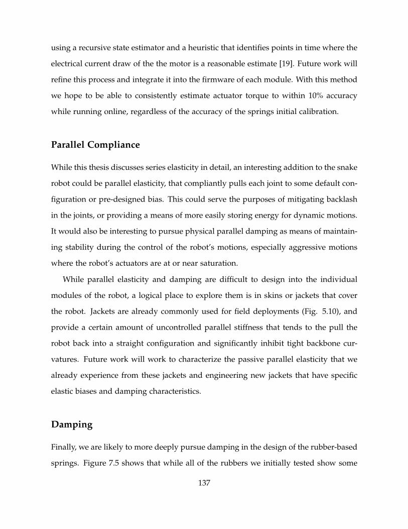
using a recursive state estimator and a heuristic that identifies points in time where the

electrical current draw of the the motor is a reasonable estimate [19]. Future work will

refine this process and integrate it into the firmware of each module. With this method

we hope to be able to consistently estimate actuator torque to within 10% accuracy

while running online, regardless of the accuracy of the springs initial calibration.

Parallel Compliance

While this thesis discusses series elasticity in detail, an interesting addition to the snake

robot could be parallel elasticity, that compliantly pulls each joint to some default con-

figuration or pre-designed bias. This could serve the purposes of mitigating backlash

in the joints, or providing a means of more easily storing energy for dynamic motions.

It would also be interesting to pursue physical parallel damping as means of maintain-

ing stability during the control of the robot’s motions, especially aggressive motions

where the robot’s actuators are at or near saturation.

While parallel elasticity and damping are difficult to design into the individual

modules of the robot, a logical place to explore them is in skins or jackets that cover

the robot. Jackets are already commonly used for field deployments (Fig. 5.10), and

provide a certain amount of uncontrolled parallel stiffness that tends to the pull the

robot back into a straight configuration and significantly inhibit tight backbone cur-

vatures. Future work will work to characterize the passive parallel elasticity that we

already experience from these jackets and engineering new jackets that have specific

elastic biases and damping characteristics.

Damping

Finally, we are likely to more deeply pursue damping in the design of the rubber-based

springs. Figure 7.5 shows that while all of the rubbers we initially tested show some

137

hysteresis, neoprene rubber has significantly more hysteresis and damping. Since the

initial goal was to achieve torque control, we decided to use 50A durometer natural

rubber due to its greater linearity. Now that we have demonstrated that locomotion

is possible with the level of accuracy we currently possess, we plan to examine if

using neoprene rubber can provide additional stability benefits, while still maintaining

torque sensing that is accurate enough for locomotion.

11.4 Low Impedance Motions

The work on low-impedance locomotion for snake robots is in a preliminary stage.

We feel that this thesis at least demonstrates that SEAs with moderate torque sensing

accuracy can still be used to achieve useful compliant motions, and future work is

continuing on all three of the methods that were presented in Chapter 9.

Compliant Roll-In-Shape

The controller presented in Section III depends solely on the curvature of the robot

along its backbone and serves as a general starting point for creating more complex

motions. One interesting avenue of future work will involve tuning the commanded

torque based on the overall shape of the robot. For example, a useful motion could be

rolling along the ground but being compliant to small obstacles like rocks and gaps.

The controller presented here tends to have the robot roll up around the obstacle, rather

than roll over it. One strategy could involve adjusting the desired torques to allow

tighter curvatures in one dimension and stiff curvatures in an orthogonal dimension,

based on the robot’s overall shape [77]. Alternatively, the controller could be adjusted

using the estimated pose of the robot [79].

138

Low-Impedance Sliding

This control strategy is perhaps the most interesting because it seems to closely mimic

the motions of biological snakes. Work will continue on tuning the controller, allowing

more informed steering of the head of the robot. The simple controller presented in

Section IV works well in confined spaces, but tends to perform poorly when the shape

is not well-constrained. We are currently exploring additions to the controller, for ex-

ample schemes that encourage continuous motion, or encourage non-zero derivatives

in backbone curvature.

Finally, the characteristics of the skin of the snake play an important role dur-

ing sliding motion. Therefore we are investigating other low-friction, or possibly

directional-friction, skins to aid in sliding over a wider range of surfaces. If cou-

pled with forms of active propulsion along the spine of the robot, like tracks or small

wheels, it is possible that this control strategy could provide exceptional mobility over

rough terrain.

Empirical Gait Construction

We presented initial results in constructing a low-impedance version of the slithering

gait. Although the recording and playback of joint torques to achieve low-impedance

locomotion is a very limited method, the approach does have the advantage that can be

applied to all existing position-controlled gaits or motions. In addition to examining

different gaits, future work will involve generalizing and parameterizing these new

low-impedance motions, so that they can be easily adjusted online, like traditional

position-controlled gaits the we currently use. One approach we are pursuing involves

modeling the motion using simple friction models, like viscous friction in cartesian

space, to determine the appropriate feedforward torques for compliant locomotion.

Another approach will investigate combining the curvature derivative control with our

139

position controlled gaits, so that a control law on the curvature derivative becomes the

primary driver of the robot’s shape changes. Finally, there existing work in machine

learning on deriving continuous trajectories and controllers from demonstration that

could serve as another interesting approach [18, 36].

140

Part IV

Appendix

141

Appendix A

The Importance of Body Frame

Despite the success of a number of groups in developing gaits and motions for snake

robots, a significant, yet overlooked, challenge remains: how to represent a snake

robot’s motion. In particular, defining a body frame which intuitively describes the

robot’s motion in the world is difficult. To illustrate this problem, consider a simple

two-wheeled differential drive robot with a body frame fixed to the center of the robot’s

chassis. Operating such a device is easy because the notions of ‘forward’ or ‘up’ are

clearly defined, and the robot’s wheels propel it smoothly through the world. Put in

more technical terms, the robot’s definition of pose is independent from its internal

shape changes (the turning of the wheels), and its controls, which are executed in the

body frame, map intuitively into a world frame. With snake robots, an operator can

still control the robot with some sense of its position and orientation by simply looking

at the robot. However, the intuition for this frame lies solely with the operator, and is

drawn from observing the robot as a whole rather than any individual link (Fig. A.1).

A major contribution of this thesis is to formally define a body frame that embodies

this intuition. In particular, we show that using a body frame whose origin is the

robot’s center of mass and whose axes are aligned with the robot’s principal moments

of inertia is one where the intuitive notions of position and orientation prevail. We

143

Figure A.1: An example of an operator’s intuitive notions of orientation for the snake robot.The red solid arrow indicates the intuitive definition of up/forward. The green dashed arrowindicates the intuitive direction of sideways.

refer to this frame as a virtual chassis because, like the chassis of a car, it isolates a

robot’s internal shape changes from its external motions, allowing us to think of snake

robots more like wheeled vehicles.

A.1 Prior Work

Using an averaged approximation of a system as a way of providing intuition to a

system’s analysis and control has been explored in other contexts. For planar swim-

ming systems, Shapere and Wilczek [85] use the center of mass and principal axes

to define body frames for irregularly shaped bodies. Zafa and Dubowsky simplified

kinematic planning and workspace analysis for a robotic manipulator floating in space

by using a virtual ground located point at the system’s center of mass [96]. In the field

of humanoid robotics, Kajita et al. [42] use the pseudo-inverse of the inertia matrix

to quickly generate whole body motions where the linear and angular momenta are

144

controlled. However, in that work the body frame for the robot is always able to be

referenced to some fixed point in the world (e.g., a foot on the ground that is assumed

not to move in the world frame). This convenience is not possible with snake robots

as the ground contact is much more complex, and it is difficult to accurately estimate

what points on the robot, if any, are stationary in the world at a given point in time.

Similar perspectives can also be found in the world of computer vision. Yezzi and

Soatto use similar techniques to match shapes based on overall similarity [108]. There

is also a large body of work using SVD to match and characterize image features

[13, 69, 82].

The virtual chassis is in many ways inspired by the work of our group [28], who

demonstrate that a good choice of body frame can greatly simplify motion planning for

planar systems. By exploiting a system’s known dynamics they are able optimize the

coordinate frame to be one in which a locomoting system moves the least in response

to changes in its shape. Using these minimum perturbation coordinates, they are able

to identify effective gaits by representing the system dynamics as geometric functions

over the system’s shape space. While we lack the specific constraints needed to define

optimal coordinate frames in their manner, our work draws on their observation that

their optimal body frame is often aligned with the intuitive notions of center of mass

and mean orientation.

A.2 Definition

The overall procedure for calculating the virtual chassis involves continually aligning

the body frame with the robot’s principle moments of inertia. Specifically, this is done

by taking the singular value decomposition (SVD) of the positions of all of the robot’s

links with respect to the robot’s center of mass at discrete time steps as the robot exe-

cutes the gait. This process can also be thought of as repeatedly performing principal

145

Figure A.2: An example of an arbitrary initial body frame for the robot that is fixed to the headlink.

component analysis (PCA) on zero-mean data.

A.2.1 Calculating the Virtual Chassis Body Frame

Given an arbitrarily chosen body frame, such as one fixed to the head link (Fig. A.2),

we can use standard kinematics to calculate the poses of all the links on the robot with

respect to this frame [63]. We then find the translation and rotation from this initial

frame to the frame aligned with the principle moments of inertia taken about the center

of mass. We then transform the pose of each link of the robot from the initial frame to

this new frame, thereby representing the robot’s pose in the virtual chassis.

The first step is to find the geometric center of mass of the robot x, y and z in

the initial frame. We then construct a data matrix of the positions of the links pi,

subtracting out the center of mass. This matrix, P will be of size n×3, where n is the

number of links and each row i corresponds to the ith link in the robot,

pi =

[xi − x yi − y zi − z

](A.1)

146

P =

p1

...

pn

. (A.2)

Now that the origin of the initial coordinate frame is at the center of mass, the next

step is to find a rotation such that the principal axes of the body frame are aligned

with the principal moments of inertia of the link positions around the center of mass.

To find this rotation we take the SVD of P. SVD decomposes this matrix into three new

matrices,

USVT = P. (A.3)

In the decomposition, U and V are unitary matrices whose columns are respectively

the left and right singular vectors of P. The columns of U are eigenvectors of PPT,

meaning that they form an orthonormal basis in Rn. Likewise, the columns of V are

eigenvectors of PTP and form an orthonormal basis in R3. This means that V serves

as a rotation matrix that describes the orientation of the coordinate frame aligned with

the principal moments of inertia, described in initial coordinate frame. The diagonal

elements of S are the singular values of P. They correspond to the square roots of the

eigenvalues of PTP and describe the magnitudes of the principal moments of inertia.

More detail on SVD can be found in [93].

A technical detail to note about SVD is that V is only unique up to a reflection

about each singular vector [6]. To ensure right-handed coordinates, at each timestep V

is modified such that the third singular vector is defined to be the cross product of the

first and second singular vectors. To avoid sign flips in V across later timesteps, we

respectively enforce positive dot products between the first and second singular vectors

at the current timestep and those of the previous timestep. As long as the same initial

body frame is used to generate P at both timesteps and the shape changes between

147

timesteps are not drastic, the rotation described by V is stable and unambiguous in

sign.

Combining the rotation matrix V with the center of mass p we have the homoge-

neous transform that describes the pose of the virtual chassis with respect to the initial

body frame,

T =

V p

0 1

. (A.4)

The last step is to transform the pose of each link in the robot to the virtual chassis

body frame. If the pose of each link is described by a homogeneous transform, left-

multiplying each link’s transform by T−1 now represents its pose in the virtual chassis

body frame.

A.3 Implementation

Our lab has developed a variety of gaits for our snake robots, including sidewinding,

rolling, pipe crawling, and pole climbing (Fig. 2.4). For each of these gaits, we demon-

strate calculating the virtual chassis via SVD as outlined in the previous section. Note

that this general procedure can be applied to any body shape that has distinct principle

components, including non-cyclic motions and transitions between gaits. For gaits de-

signed specifically to traverse pipes, we can further refine the virtual chassis to exploit

the structure of the robot’s shape, better aligning the body frame with centerline of the

pipe.

148

Figure A.3: An example of the approximate axes of the virtual chassis for the sidewinding gait.

A.3.1 Sidewinding

The sidewinding gait (Fig. A.3). is characterized by a series of lateral and dorsal

undulations that form a rolling tread [7, 61]. This motion corresponds to a phase offset

of π/4 in the serpenoid equations (2.1). The overall shape of the robot in sidewinding

can be described as a helix with an elliptical cross-section. This body shape has the

property that the longest, middle, and shortest principal components of the shape are

clearly defined and are orthogonal.

For sidewinding, the procedure for calculating the virtual chassis follows the gen-

eral procedure from Section 3. At each new timestep, a new P is calculated from the

robot’s joint angles and a new body frame is defined. A comparison of sidewinding

motion in an initial head-fixed body frame and the virtual chassis body frame is shown

in Fig. 4.2 of Chapter 4. Note that the motion of the robot in virtual chassis body frame

captures the ‘rolling tread’ motion of the gait, compared to the side to side motion that

is apparent in a fixed body frame.

149

Figure A.4: An example of the approximate axes of the virtual chassis for the rolling gait.

A.3.2 Rolling

In the basic rolling gait the robot forms a static backbone shape, consisting of an arc of

constant curvature, and then rolls within that shape (Fig. A.4). This constant curvature

corresponds to setting the spatial frequency ν in (2.2) to 0, and setting the phase offset

between the lateral and dorsal joint angles, δ from (2.1) to π/2 radians.

As the robot cycles through the gait over flat terrain, the arc remains level on the

ground and the robot rolls either toward or away from the center of the arc. Like

sidewinding, the shape of the robot in rolling has clearly defined longest, middle,

shortest dimensions to its shape.

For this gait we align the first, second, and third principal moments of inertia re-

spectively with the x, y, and z axes of the body frame. The procedure for calculating

the virtual chassis for rolling follows the general procedure. A comparison of the mo-

tions of the rolling gait in an initial head-fixed body frame and the virtual chassis body

frame is shown in Fig. A.5. Note that the motion of the robot in virtual chassis body

frame matches the gait’s internal twisting motion, compared to the sweeping motion

that is apparent in a fixed body frame.

150

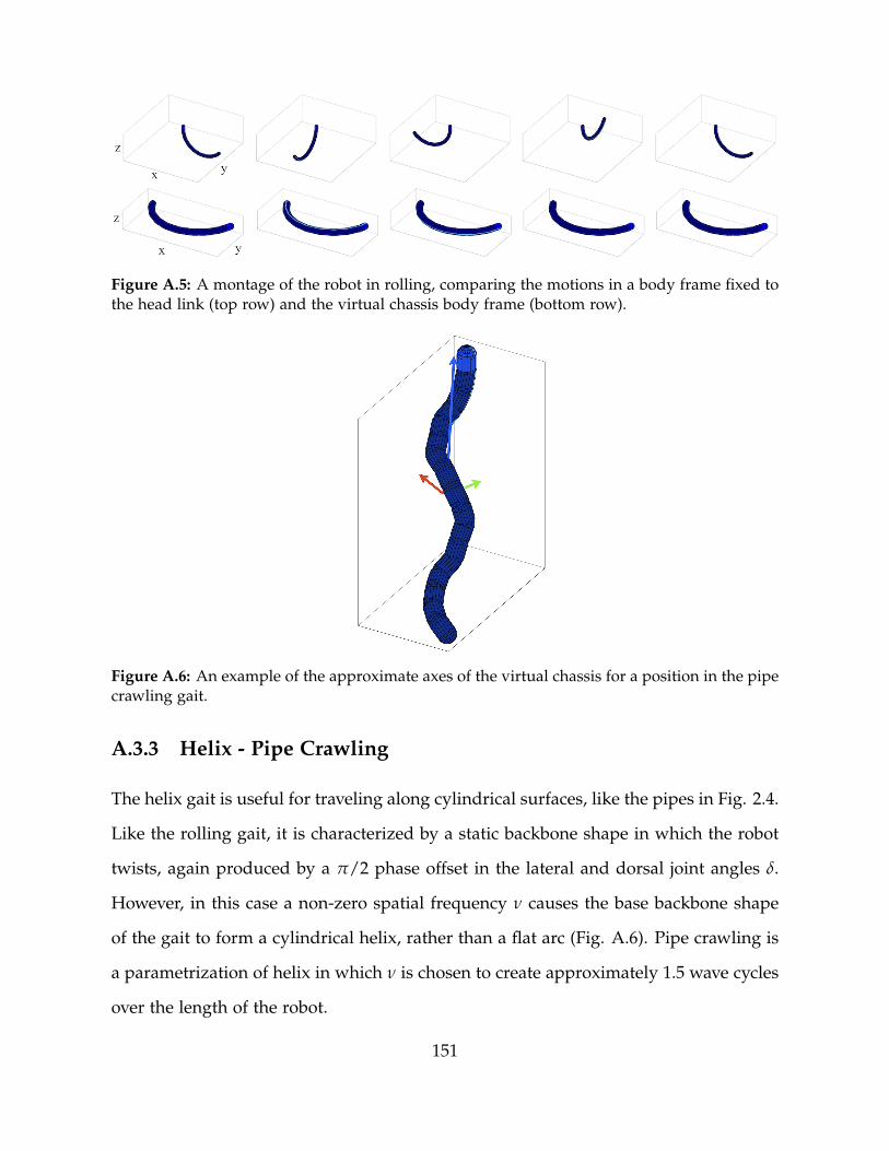
Figure A.5: A montage of the robot in rolling, comparing the motions in a body frame fixed tothe head link (top row) and the virtual chassis body frame (bottom row).

Figure A.6: An example of the approximate axes of the virtual chassis for a position in the pipecrawling gait.

A.3.3 Helix - Pipe Crawling

The helix gait is useful for traveling along cylindrical surfaces, like the pipes in Fig. 2.4.

Like the rolling gait, it is characterized by a static backbone shape in which the robot

twists, again produced by a π/2 phase offset in the lateral and dorsal joint angles δ.

However, in this case a non-zero spatial frequency ν causes the base backbone shape

of the gait to form a cylindrical helix, rather than a flat arc (Fig. A.6). Pipe crawling is

a parametrization of helix in which ν is chosen to create approximately 1.5 wave cycles

over the length of the robot.

151

Figure A.7: A montage of the robot in pipe crawling, comparing the motions in a body framefixed to the head link (top row) and the virtual chassis body frame (bottom row).

The shape of the robot in pipe crawling has a clearly defined longest direction,

corresponding to the first principal moment of inertia. However, in this gait the second

and third moments of inertia are less distinct. This makes intuitive sense, since for a

true cylinder the second and third moments are exactly equal, due to symmetry about

the cylinder’s axis. Since the robot consists of a finite number of links, significant

asymmetry is present, and SVD will still find an unambiguous solution for the virtual

chassis.

As with the gaits discussed so far, the resulting body frame using the general pro-

cedure isolates the robot’s internal and external motions. However, since this gait is

used specifically for locomoting on the inside of pipes (bottom left of Fig. 2.4), we

can exploit the known constraints of the environment and define a more useful body

frame that is better aligned with the true centerline of the robot’s helical shape (as well

as centerline of the pipe).

To find the true centerline of the robot, we take the initial solution from SVD and

use it as the starting point of optimization using the Nelder-Mead simplex search [64].

Intuitively, we would like to minimize the difference of the distances of all the links in

robot to some centerline. If we define this centerline as the set of points, `(s) = a + vs,

152

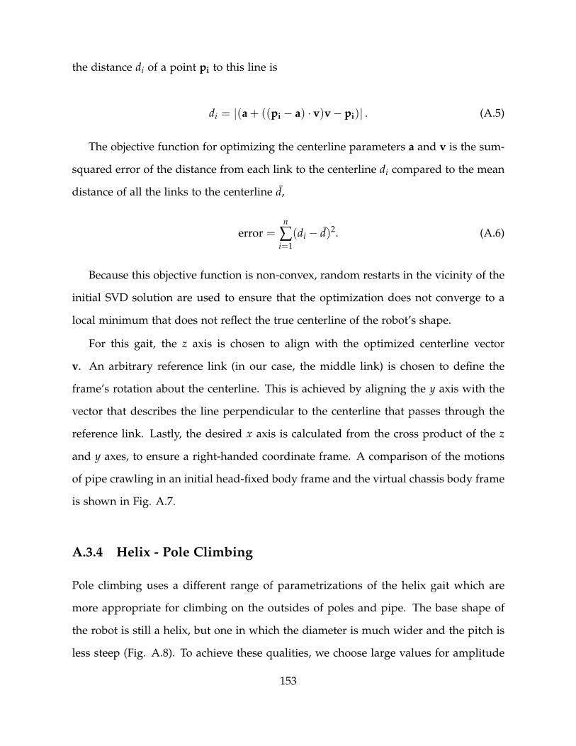
the distance di of a point pi to this line is

di = |(a + ((pi − a) · v)v− pi)| . (A.5)

The objective function for optimizing the centerline parameters a and v is the sum-

squared error of the distance from each link to the centerline di compared to the mean

distance of all the links to the centerline d,

error =n

∑i=1

(di − d)2. (A.6)

Because this objective function is non-convex, random restarts in the vicinity of the

initial SVD solution are used to ensure that the optimization does not converge to a

local minimum that does not reflect the true centerline of the robot’s shape.

For this gait, the z axis is chosen to align with the optimized centerline vector

v. An arbitrary reference link (in our case, the middle link) is chosen to define the

frame’s rotation about the centerline. This is achieved by aligning the y axis with the

vector that describes the line perpendicular to the centerline that passes through the

reference link. Lastly, the desired x axis is calculated from the cross product of the z

and y axes, to ensure a right-handed coordinate frame. A comparison of the motions

of pipe crawling in an initial head-fixed body frame and the virtual chassis body frame

is shown in Fig. A.7.

A.3.4 Helix - Pole Climbing

Pole climbing uses a different range of parametrizations of the helix gait which are

more appropriate for climbing on the outsides of poles and pipe. The base shape of

the robot is still a helix, but one in which the diameter is much wider and the pitch is

less steep (Fig. A.8). To achieve these qualities, we choose large values for amplitude

153

Figure A.8: An example of the approximate axes of the virtual chassis for a position in the poleclimbing gait.

Figure A.9: A montage of the robot in pole climbing, comparing the motions in a body framefixed to the head link (top row) and the virtual chassis body frame (bottom row).

A, and smaller values of spatial frequency ν.

As in pipe crawling, the coordinate frame can again be optimized beyond what is

provided by SVD. In fact, it becomes even more beneficial as the misalignment of the

first principal moment of inertia with the true centerline of the robot’s helix is much

more pronounced. This effect is primarily attributable to the ‘longest’ direction of the

robot’s shape becoming more ambiguous, as the increased diameter of the helix starts

to approach the overall length of the helix. The virtual chassis body frame for pole

climbing is calculated with the same secondary optimization as pipe crawling, and the

result is shown in Fig. A.9.

154

A.3.5 Real-time Implementation

Calculating the virtual chassis using the SVD procedure can easily be performed in

real time. However, when using the refined virtual chassis body frame in pipes, the

secondary optimization significantly slows the body frame calculations. To address

this limitation, we precompute lookup tables for the body frames or calculate the the

SVD-based virtual chassis for an idealized shape [17], both of which are based on

knowledge of the gait parameters. For pipe crawling and pole climbing, we require

three lookup parameters from the gait equations (2.1) and (2.2): temporal position in

the gait cycle ωt, amplitude A, and spatial frequency ν. To find the gait parameters

that best describe the robot’s shape, we can fit them to the to feedback joint angles in

real time using an extended Kalman filter (EKF), which is detailed in Chapter 5.

A.4 Ambiguous Shapes

In practice, the generic SVD-based virtual chassis algorithm is more useful due to its

ability to be calculated completely independently of the robot’s control framework.

However, instabilities in the virtual chassis arise when principle components of the

robot’s shape become ambiguous. These instabilities can cause the pose of the virtual

chassis body frame to change drastically with respect to the pose the robot. This is

problematic to state estimators, like those presented in Chapter 4, that rely on the

virtual chassis as an approximate separation of the robot’s internal and external shape

changes.

Ambiguous shapes of the robot can be divided into two classes. The first class is

where the magnitudes of any two principal components of the robot’s shape are similar

but non-zero. This can occur on the first and second principal components when

transitioning between classes of gaits, like from rolling to pole climbing, as shown in

155

Figure A.10: An example of problematic shapes for the virtual chassis. Note the large changesof motion that occur between the first and second frames and the third and fourth frames, eventhough there is relatively little difference in the robot’s shape

Fig. A.10. It can also occur on the second and third principal components during

internal pipe crawling.

The second class is where two principal components of the robot’s shape are similar

and close to zero, which only happens when the robot forms a straight line. In this

case the shape of the robot is truly degenerate and extremely unstable if the shape of

the robot undergoes even slight shape changes. While this shape is not typically used

in locomotion, it is the default shape that the robot assumes on power up, so avoiding

these instabilities is desired if at all possible.

A.5 An Alternative Virtual Chassis

One way of addressing instabilities of of the first class is to define a different metric

for the definition of the virtual chassis body frame. Rather than find the principle

components of the robot’s shape, an alternative method is to align the robot’s overall

shape across subsequent time steps. This task has been studied in aerospace fields

and is known as Wahba’s problem [98]. Interestingly, a solution to this problem is also

based on SVD [59].

Wahba’s problem seeks find the minimal rotation that aligns two sets of vector

observations. In three dimensions, 3 or more non-collinear points each need to be

156

observed in two different frames. These n points are arranged in the matrices A3×n

and B3×n, corresponding respectively to the two frames. These matrices are multiplied

to form a 3× 3 correlation matrix

C = ABT. (A.7)

We then take the singular value decomposition (SVD) of C,

C = USVT. (A.8)

In SVD, U and V are orthonormal bases that can be thought of as rotation matrices,

and S can be considered a scaling matrix. The optimal rotation, R, to align the sets of

points A and B is found by simply replacing the matrix S with a diagonal matrix of

ones, except the lower-right term which is the product of the determinants of U and V,

R = VMUT (A.9)

M = diag([1 1 det(U)det(V)]). (A.10)

For our robot, A and B are the positions of each module of the robot in the body

frame. Using this method as our virtual chassis will result in a body frame that is

no longer aligned with the principle components of the robot’s overall shape, but will

instead minimize the disturbance in subsequent shape changes, as shown in Fig. A.11.

Calculating the robot’s body frame in this way means that the body frame will drift

over time with respect to the robot’s overall shape, losing some of the intuitive benefits

of the shape-aligned virtual chassis. However, this alternative body frame has the

advantage that it is stable for any shape of the robot, except the single case where all

the robot’s links are collinear. This makes it more attractive for behind-the-scenes tasks

157

Figure A.11: A comparison of different methods of calculating the virtual chassis for a shapethat has ambiguous principal components. The top row shows the virtual chassis computedusing the robot’s principal components. The bottom row shows the virtual chassis calculatedby matching the individual links of successive shapes.

like improving filtering and state estimation where human intuition is less important.

A.6 Future Work

The virtual chassis proven itself to be a useful tool for intuitively understanding the

motions of snake robots, without simulating the physics of the robot in the world or

running the motions on an actual robot. Additionally we continue to believe that a

careful choice of body frame can have computational benefits for tasks like state esti-

mation and motion planning. For these reasons, we suggest some areas of future work

extending the capabilities and formalizing the implementation of the virtual chassis.

A.6.1 Dynamic Motions

The virtual chassis in its current form only considers the kinematic configuration of the

robot. That is to say that the velocities of the different links of the robot, or the energy of

158

its motion, have no bearing on the calculation of the body frame. While this assumption

works well for snake robots, extending the virtual chassis to other robots might bring

the need to account for high speed motions or situations where the robot has significant

inertia. For systems like walking humanoids or running quadrupeds, dynamic effects

play a much larger role in separating a robot’s internal shape changes and external

motions. Extending the virtual chassis to take into account a robot’s dynamics was

beyond the scope of this thesis. However, methods for humanoid robots that take into

account the total momentum of the robot [42] may provide a good starting point.

A.6.2 Remaining Instabilities

Both versions of the virtual chassis that we have developed are unstable for the case

where all the links of the snake robot are collinear. The simplest strategy mitigate this

problem is to switch to a body frame fixed to some module in the robot when the

magnitudes of the second and third principal components of robot’s shape become

small. The primary challenges with this method are choosing when to switch to and

from a fixed body frame, which fixed frame to choose, and how to gracefully handle

the transition between frames.

To determine when to switch to a fixed frame, one could envision a heuristic that

identifies when the virtual chassis is becoming unstable, based on a ratios of the rel-

ative weights of the principal components of the robot’s shape, the diagonal of S in

(A.3). Based on these ratios, we can gradually shift to using using a fixed frames when

the shape is near a singularity and then back to the virtual chassis when it is once

again stable.

159

A.6.3 Incorporating Inertial Sensing

Finally, it is possible to rely on the inertial sensors of the robot to inform the calculation

of the virtual chassis. Inertial data has already been incorporated into resolving an up-

down ambiguity in the virtual chassis for generating approximate motion models for

the snake robot [16]. Even though using inertial data in the definition of the body

frame no longer relies solely on the shape of the robot, this could be practical method

of generating a useful averaged body frame in the field since this sensor data is freely

available any time the robot is running. In Kalman the context of the filtering presented

in Chapter 4, this could come in the form of using a virtual chassis inertial sensors to

directly propagate the state of the robot’s pose at a high update rate, and performing

the full EKF or UKF update a lower update rate for computational efficiency.

160

Appendix B

Design and Architecture of a Series

Elastic Snake Robot

Like previous generations of our robots, the SEA Snake consists of a number of identical

1-DOF modules in which the actuated axes are oriented in the lateral and dorsal planes

of the robot. Most notably, this latest generation contains a series elastic actuator

in each module. This enables compliant motion over rough terrain and fine torque

control on each joint. Additionally, each module contains a 32-bit processor and 100

Mbps Ethernet data bus, a 400X improvement in bandwidth over the RS-485 serial

communications of our previous robot, the Unified Snake [102]. The modules also have

greater torque output, improved sealing, and a rugged tool-free interface. Table B.1

presents the specifications of the SEA Snake robot.

B.1 Mechanical Overview

Each module possesses a self-contained 1-DOF joint, allowing for a full 180◦ of rotation.

Modules are interfaced together and alternately aligned in accordance with the robot’s

lateral and dorsal planes. A typical robot consists of 16 modules linked together, with

161

Table B.1: Overview of SEA Snake specifications.

DimensionsDiameter: 5.1 cmLength (module): 6.4 cmLength (full 16 module robot): 1.174 m

MassModule: 205 gFull 16 module robot: 3.657 kg

ActuationMax Torque: 7 N-mMax Speed: 33 RPM

Power48 VCurrent (resting): 40 mACurrent (max): 600 mA

Communication 100 Mbps Ethernet

Sensing

Angular Position and VelocityOutput Torque3-axis Accelerometer3-axis GyroTemperatureVoltageCurrent

162

Figure B.1: Photo of a SEA Snake Module. The module is 5 cm (2 in.) in diameter and providesa 1-DOF rotary motion of +/- 90◦.

unique head and tail modules.

A driving design requirement of the SEA Snake was ease of customization. In

addition to the 16 rotary DOF design, modules can be added, removed, interchanged,

or replaced with novel mechanisms. Any device meeting the interface requirements

can be included in the chain.

B.1.1 Motor-Geartrain

The SEA Snake modules are driven by a modified Maxon EC 20 flat motor with a

nominal speed of 9300 RPM. The steel pinion gear on the motor’s output shaft trans-

fers rotation through a geartrain containing 3 steel and brass compound gears. The

cumulative gear ratio is 349:1 to create high-torque joints. This motor and geartrain

combination provides a maximum output torque of 7 N-m and a maximum speed of

33 RPM.

163

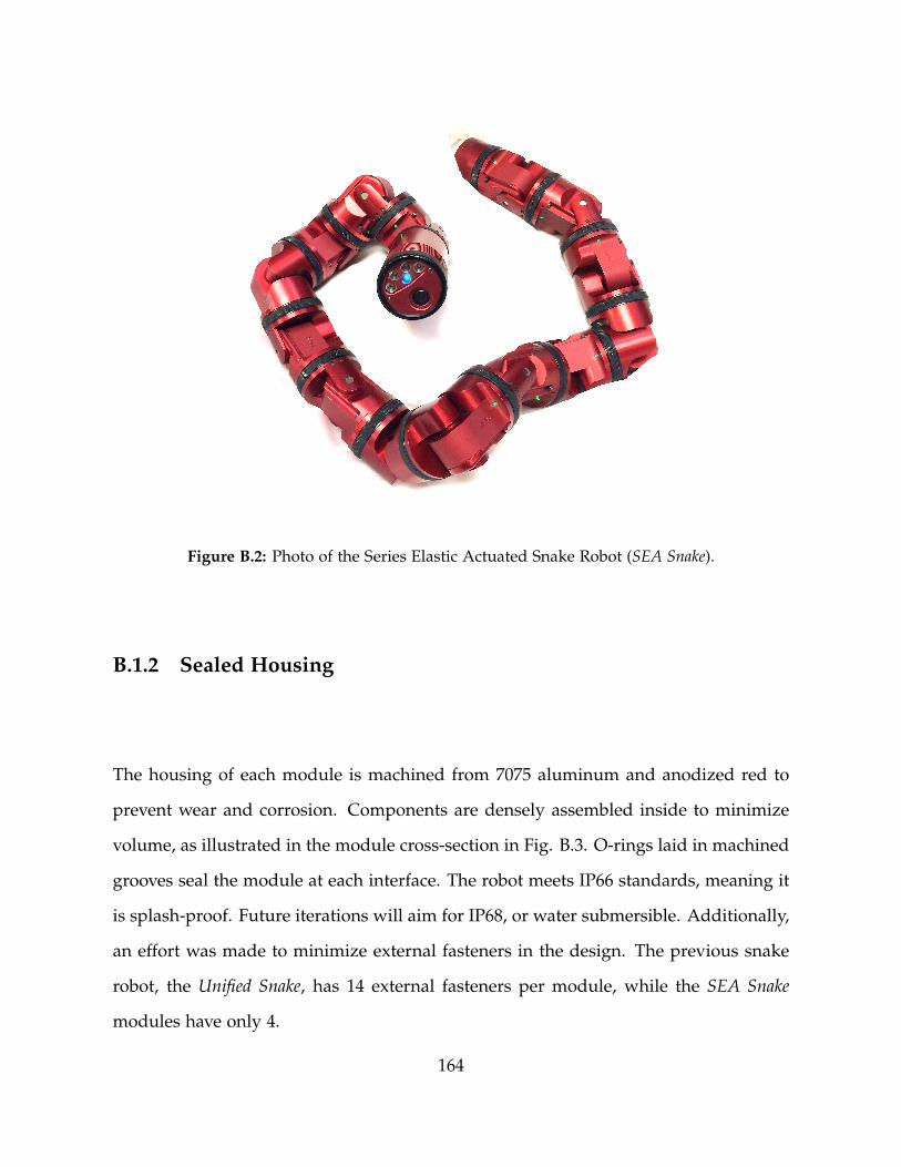
Figure B.2: Photo of the Series Elastic Actuated Snake Robot (SEA Snake).

B.1.2 Sealed Housing

The housing of each module is machined from 7075 aluminum and anodized red to

prevent wear and corrosion. Components are densely assembled inside to minimize

volume, as illustrated in the module cross-section in Fig. B.3. O-rings laid in machined

grooves seal the module at each interface. The robot meets IP66 standards, meaning it

is splash-proof. Future iterations will aim for IP68, or water submersible. Additionally,

an effort was made to minimize external fasteners in the design. The previous snake

robot, the Unified Snake, has 14 external fasteners per module, while the SEA Snake

modules have only 4.

164

Figure B.3: CAD model cross-section of a SEA Snake module.

B.1.3 Mechanical Interface

The intermodular interface features a rugged, tool-less design. Modules are aligned

with dowel pins and matching recesses. A freely-spinning threaded collar, held in

place by a retaining ring, is turned by hand to lock adjacent modules together. An

electrical connection is made between two modules with spring-pin connectors on the

interface board touching target areas on the control board.

O-rings seal the collar at both ends. Modules can be connected and disconnected

quickly and repeatedly. The connections are secure and resist shock and stress. Any

device with matching threads, 48V and Ethernet compatibility can be interfaced with

a module, allowing for freedom of design and customization.

165

Figure B.4: Photo of the modular SEA Snake interface. Dowel pins provide alignment while thethreaded collar mechanical secures and seals the modules. The electrical connection is madewith spring-pin connectors touching target areas on the control board.

B.1.4 Series Elasticity

The SEA Snake features series elastic actuators. A rubber elastomer bonded between

two rigid plates is torsionally sheared during actuation [80]. The elastomer’s tapered

conical cross section shown in Fig. B.5 is similar to the constant-shear-stress design

introduced in [80]. The spring here is different in that it is molded directly to the

output gear of our geartrain. The rigid plate on top is then attached to the output shaft

of the system through a number of pins. Another plate is swaged onto this assembly

in order to keep the output gear and output shaft aligned with the rest of the geartrain.

The elastomer is molded from Natural Rubber of Shore A Durometer 50. As a tor-

sional spring, its stiffness is roughly characterized by a spring constant of 12 N-m/rad

and a maximum rotational deflection of approximately 0.6 radians. Our research is

currently exploring ways to estimate the output torque from the elastomer deflection

and how to calibrate its parameters online [19].

166

Figure B.5: CAD model cross-section of a module’s output shaft assembly. The rubber isbonded to the tapered surfaces of the output gear and top washer. The output shaft is hollow,allowing wires to pass through the center of rotation of the module.

B.1.5 Head and Tail Modules

Both a head and tail module were designed utilizing the custom modular interface and

they are pictured in Fig. B.6. In addition to providing their specialized functions, these

modules demonstrate the potential for the use of other modules that could easily be

integrated into the SEA Snake system.

The head module includes a high-definition camera to provide the user with a live

video feed while the four LEDs are available for illuminating darker environments. The

head module housing is designed with fins to increase surface area and improve heat

transfer from the electronics to the surrounding environment. The LEDs are protected

by an o-ring sealed acrylic window while the camera’s lens is protected by an o-ring

sealed sapphire glass window.

In order to connect a tether to the snake, we custom-designed a tether connector

that is sealed and load-bearing. The connector uses keys and keyways to provide

a quick and very easy blind connection. Additionally, there are spring-loaded pins

within the connector which ensures that the connector’s housing bears all of the load.

The tail has this connector as well as a slipring integrated within its design.

167

Figure B.6: Photos of SEA Snake head and tail modules.

B.2 Electronics Overview

While the electronics in the previous generation robot were robust, we set out to de-

sign the SEA Snake electronics with a focus on ease of development to facilitate future

research, such as more advanced control algorithms and onboard sensor fusion. To this

end, we moved from an 8-bit AVR processor to a 32-bit ARM Cortex M4F running at 7X

the clock speed. We also wanted to enable higher frequency external control and sen-

sor feedback and to move from analog to digital video. To satisfy these increased data

requirements we moved from a 250kbps RS-485 bus to a switched 100Mbps Ethernet

network.

B.2.1 Communication

One hindrance to adopting Ethernet in embedded devices is the size of the isolation

transformers typically required. Our solution was to integrate a three port Ethernet

switch into each module. This keeps the wire length down to a few centimeters, which

is far shorter than the electrical propagation distance during a single 10ns bit period.

168

Cortex M4F

SPI

I2C

DAC

PWM

RS-485 RS-485

3 PortEthernet Switch

Encoders

Current

Voltage

Temperature

Inertial

Sensors BrushlessMotor Driverand Current

MotorHALL

3.3VSwitchingRegulator

5V BoostRegulator

48V 48V

D

u

t

y

C

y

c

l

e

R

e

f

e

r

e

n

c

e

C

u

r

r

e

n

t

100MbpsEthernet

100MbpsEthernet

Full DuplexRS-485Serial

Full DuplexRS-485Serial

Figure B.7: Module Electronics Block Diagram.

This allowed us to relax the controlled impedance requirements, and to replace the

transformer isolation with capacitive isolation, which has a far smaller PCB footprint.

We do provide transformer isolation in the tail module to insure signal integrity over

the tether.

In addition to the Ethernet link each module has a full duplex differential serial link

to each of its immediate neighbors for future uses including ‘autonumbering’ of the

modules. We have implemented a system in which the modules communicate their IP

address to their immediate neighbors and the robot is able to self-discover the order in

which the modules are connected. This greatly aids in field maintenance and flexibility

of the robot as a research platform.

B.2.2 Electrical Interface

On the previous snake robot design the module interface was along the axis of rotation,

requiring us to create a custom connector to fit around the coaxial magnet used for

169

position feedback. The SEA Snake design moves the module interface away from the

axis of rotation which has many advantages for the electrical interconnection. Because

we have more space for the interconnection we use spring contacts that mate with gold

plated PCB pads instead of very thin pins. This arrangement is much more tolerant to

misalignment, eliminating the problem of bent or broken pins. The new design also

moves the intermodule wiring terminations as far as possible from twisting motion

caused by joint rotation, greatly reducing the risk of fatigue failures at the crimp/solder

connections.

B.2.3 Motor Control

The SEA Snake is our first generation to include a brushless motor. We drive the motor

with an integrated single chip solution to which we add current sensing. The series

elastic member also required the addition of a second magnetic rotation encoder which

allows us to measure the deflection. We use a 48V system voltage and 36V motor

combined with thermal modeling to allow the system to safely exceed the continuous

operation ratings of the motor for brief periods.

B.2.4 Sensors

Every generation of our snake robot has benefited from rapid development in inertial

sensor technology driven by consumer electronics, with the current generation featur-

ing a single chip solution with 3-axis gyro, 3-axis accelerometer, and 3-axis magnetome-

ter which costs 1/3 the price of the 2-axis gyro from early in the previous generation.

We retained all the other sensing present in the previous generation including voltage

and temperature monitoring, but we also added a current sensor to measure the con-

sumption of the entire module in addition to the motor current measuring circuit. This

generation also adds externally visible PWM controlled RGB LEDs without sacrificing

170

environmental sealing to provide immediate feedback on module status.

B.2.5 Camera Head

The use of Ethernet as the standard communication interface between modules enables

the use of readily available, IP security cameras as the basis for the head module

of the snake. In the Unified Snake architecture, the video was transmitted over a

dedicated, analog bus that supported only standard definition video. By moving to

an Ethernet-based camera, the video stream is piped over the same set of cabling as

the motion control commands. In addition, the bandwidth that is needed to transmit

a high definition video stream is a fraction of the total bandwidth available on the

system, paving the way for the use of multiple cameras and additional sensors.

The camera module that has been designed to be used for the SEA Snake is primarily

built around the circuit board and camera that were harvested from a commercially

available security camera. A custom circuit board was designed to provide power

to the camera, to support additional sensors such as an IMU and a pressure sensor,

as well as to control high-brightness LEDs for camera illumination. The camera and

electronics were packaged into a simple aluminum tube featuring the same standard

mechanical and electrical interface as the regular snake modules.

B.3 Firmware Overview

The SEA Snake robot is a research platform and is constantly reconfigured to support

new physical configurations, module types, and sensor types. In addition, researchers

with a range of experience must be able to use the platform for research in controls,

perception, and planning. To support these research goals, we developed a modu-

lar firmware that provides an API supporting both high-level and low-level control

171

abstractions.

B.3.1 OS and Hardware Abstraction Layer

The core of the firmware is an RTOS that separates the setup and upkeep of vari-

ous hardware modules into separate threads. ChibiOS/RT1 was selected due to its

out-of-the-box support for STM32 Cortex processors and a hardware abstraction layer

supporting peripherals such as Ethernet (via the lwIP2 stack), serial, analog-digital

conversion, and pulse-width modulation. Each functional component of the module

is wrapped in a C++ class abstracting its setup and configuration into a statically-

initialized singleton. This wraps over the hardware abstraction layer provided by

ChibiOS, combining multiple hardware peripherals blocks related to each component.

For example, we internally initializes a serial interface, digital IO lines, and thread-

safety, but exposes only simple read and update functions. This allows non-technical

users to safely reconfigure hardware for specific purposes.

B.3.2 Communication

Modules communicate with each other and client software via Google Protocol Buffer3

messages. Protocol Buffers define a fixed serialization format for typed data structures

that is supported across multiple computing platforms. We ported the Google C++

library for Protocol Buffers to ChibiOS to allow messages to be encoded and decoded

on the SEASnake module.

Rather than providing remote-procedure calls (RPC), we define a single “meta”-

message which defines a number of optional fields that encode module parameters

and data streams. Any computing environment with Protocol Buffer support can then

1http://www.chibios.org/2http://savannah.nongnu.org/projects/lwip/3https://code.google.com/p/protobuf/

172

interact with the snake by sending and receiving streams of these meta-messages. An

advantage of this protocol is that it is fundamentally stateless and messages can be

handled transactionally, naturally supporting multiple concurrent asynchronous con-

nections.

This protocol is exposed identically over TCP sockets, UDP sockets, and the serial

interface between modules, allowing a variety of flexible communication strategies to

be used in various situations, depending on available bandwidth, required level of con-

trol, and interface hardware. Modules can propagate local information (such as topol-

ogy) by exchanging data over the serial interface to neighboring modules, while in-

expensive “dumb” components which contain only low-speed microcontrollers can be

bridged to Ethernet via neighboring modules to implement low-cost special-purpose

functions.

B.3.3 Motion Control

Modules support angular position, velocity, and torque control through cascaded PID

control, as shown in Fig. 8.6. Each PID controller runs at 1kHz, although target set-

points may be updated less frequently, typically at 100 - 200 Hz. Independent position

and velocity outer loops generate torque commands, which are combined with a de-

sired feed-forward torque to define a setpoint for output torque which is maintained

by the inner torque controller.

The inner torque controller is able to directly compare desired and actual output

torque by directly observing spring deflection as the difference between the two en-

coder positions. This error is used to compute a PWM command to the motor which

applies appropriate torque to the input of the spring and gear train.

In the proportional controller, additional features were added to help compensate

for common geartrain nonlinearities, as illustrated in Fig. B.8. To prevent oscillations

173

−DeadZone 0 +DeadZone

−Max

−Punch

0

+Punch

+Max

Input

Outp

ut

Unmodified P−Control

Directional Punch

Effective Output

Figure B.8: The modified proportional controller, showing the effect of the deadzone and punchparameters on the output.

due to gear blacklash and sensor noise, we added a ‘deadzone’ within which errors are

assumed to be zero. To overcome geartrain stiction, a ‘punch’ factor (directional offset

represented by the blue dotted line) was added to help with stiction in the gear train.

Finally maximum output limits are also set for each controller. The dashed red line in

Fig. B.8 shows the output of a theoretical proportional controller, the black solid line

shows the output of our actual implementation. To mitigate windup of the integral

term we limit its output to the difference between the PD output and the a set output

level [67]. For example, using this method, if PD control already reaches this level the

integral term is reduced to 0.

B.3.4 Thermal Modeling

An important challenge for mobile robots is to safely extract as much performance as

possible out of their actuators. For brushless motors, the primary limitation on per-

formance is heat buildup in the motor windings [95]. We use online estimation of

each module’s motor winding temperature to fully exploit the motor’s performance

envelope beyond the continuous duty ratings. Figure B.10 shows a plot of the power

174

−0.05 0 0.05 0.1 0.15 0.2

0

0.1

0.2

time (sec)

angle

(ra

d)

Command

Actual

−0.05 0 0.05 0.1 0.15 0.2

0

1

2

3

time (sec)

ve

locity (

rad

/s)

−0.05 0 0.05 0.1 0.15 0.20

0.1

0.2

time (sec)

torq

ue

(N

m)

Figure B.9: The response of the angular position (top), velocity (middle), and torque (bottom)to a step input in position. This was performed on an unloaded module, and as such the torquereadings mostly reflect the static friction of the module’s shaft seals.

dissipation and estimated temperature of the motor windings while the motor is re-

peatedly stalled. The estimated winding temperature is based on a temperature sensor

near the motor, the sensed current draw of the motor, and a model of the internal

thermal resistances and capacitances of the motor similar to the method presented in

[94].

B.4 Conclusion and Future Work

The SEA Snake currently consists of a series of extremely capable 1-DOF modules.

However, there are a number of avenues of future work. These consist of ongoing

improvements to the existing modules, mostly in firmware, and the development of

different modules that share the electrical, mechanical, and software interfaces detailed

175

0 1 2 3 4 5 6 7 8 9 1040

60

80

100

time (sec)

tem

p (

°C

)

winding

housing

sensor

0 1 2 3 4 5 6 7 8 9 100

10

20

30

time (sec)

pow

er

(W)

Figure B.10: Top: Estimated temperature of the motor windings in a SEA Snake module, basedon the thermal model. Bottom: Dissipated motor power based on the measured current drawand the resistance of the motor’s windings.

above.

The most exciting avenue for future work will be the creation of a number of

new modules for the snake robot, based on the modular interface. Possible future

modules include different head modules with cameras and other exteroceptive sens-

ing, battery and wireless communication modules for tetherless operation, tracked or

wheeled modules for improved mobility in rough terrain, and ‘hockey puck’ modules

that expose general purpose inputs and outputs to easily test external sensors like force

sensing skins.

We feel the architecture we have developed is general-purpose enough that topolo-

gies other than a snake may be feasible. For example, connecting a number of these

modules together to a central chassis would enable the rapid prototyping of a field-

ready legged robot with torque and position control on each of its joints.

176

Appendix C

Supplemental Videos

C.1 Gait-Based Compliant Control

Compliant control overview:

https://www.youtube.com/watch?v=WeACnUE85Wc

Transitioning over different pipe diameters while pole climbing (Fig. 3.5):

https://www.youtube.com/watch?v=E30f3SlFpeQ

Holding the robot and stopping smoothly while pole climbing (Fig. 3.6):

https://www.youtube.com/watch?v=RFy1bos3LHU

C.2 Robust State Estimation

Animation of estimation for a variety of motions (Fig. 4.4):

https://www.youtube.com/watch?v=jNiROVsuHAQ

Estimation using only IMUs:

https://www.youtube.com/watch?v=y7nVvQJkjdM

177

C.3 Pipe Navigation

Navigating pipe networks in the lab:

https://www.youtube.com/watch?v=0CNQMiQnesc

https://www.youtube.com/watch?v=GFHkvW3tYbA

Deployment into a real storm sewer network:

https://www.youtube.com/watch?v=rKbVRNheKMc

C.4 Low-Impedance Motions

Demonstrations of various low-impedance motions on the SEA Snake:

https://www.youtube.com/watch?v=lZUzwNbromY

C.5 Virtual Chassis

Animations and description of the virtual chassis body frame:

https://www.youtube.com/watch?v=N13NstB5pVc

C.6 SEA Snake Robot

Overview of the features of the SEA Snake:

https://www.youtube.com/watch?v=te4M-b69fVs

178

Bibliography

[1] P. Abbeel, A. Coates, M. Montemerlo, A. Ng, and S. Thrun. Discriminative train-ing of Kalman filters. In Robotics: Science and Systems, 2005. 2.4.1

[2] A. M. Andruska and K. S. Peterson. Control of a Snake-Like Robot in an Elas-tically Deformable Channel. IEEE/ASME Transactions on Mechatronics, 13(2):219–227, Apr. 2008. 6.2

[3] J. Badger, A. Hulse, R. Taylor, A. Curtis, D. Gooding, and A. Thackston. Model-based Robotic Dynamic Motion Control for the Robonaut 2 Humanoid Robot. InIEEE/RAS International Conference on Humanoid Robotics, volume 2, Atlanta, USA,2013. 11.3

[4] D. C. Bentivegna and C. G. Atkeson. Compliant control of a hydraulic humanoidjoint. In 2007 7th IEEE-RAS International Conference on Humanoid Robots, pages483–489. Ieee, Nov. 2007. 2.4.1

[5] J. Borenstein, M. Hansen, and A. Borrell. The OmniTread OT-4 SerpentineRobotâATDesign and Performance. Journal of Field Robotics, 24(7):601–621, 2007.6.2

[6] R. Bro, E. Acar, and T. Kolda. Resolving the sign ambiguity in the singular valuedecomposition. Journal of Chemometrics, 22(2):135–140, 2008. A.2.1

[7] J. Burdick, J. Radford, and G. Chirikjian. A Sidewinding Locomotion Gait forHyper-Redundant Robots. Robotics and Automation, 3:101–106, 1993. 2.4.1, A.3.1

[8] J. G. Castrejon Lozano, L. R. Garca Carrillo, A. Dzul, and R. Lozano. Sphericalsimplex sigma-point Kalman filters: A comparison in the inertial navigation of aterrestrial vehicle. 2008 American Control Conference, pages 3536–3541, June 2008.2.4.2

[9] G. Chirikjian and J. Burdick. A modal approach to hyper-redundant manipula-tor kinematics. IEEE Transactions on Robotics and Automation, 10(3):343–354, June1994. 2.1, 2.4.1

[10] G. Chirikjian and J. Burdick. The kinematics of hyper-redundant robot locomo-tion. IEEE Transactions on Robotics and Automation, 11(6):781–793, 1995. 2.1

[11] H. Choset, K. M. Lynch, S. Hutchinson, G. Kantor, W. Burgard, L. E. Kavraki,and S. Thrun. Principles of Robot Motion: Theory Algorithms, and Implementations.MIT Press, Boston, USA, 2005. 2.3.1, 2.4.2

179

[12] H. Date and Y. Takita. Adaptive locomotion of a snake like robot based oncurvature derivatives. In IEEE/RSJ International Conference on Intelligent Robotsand Systems (IROS), pages 3554–3559, San Diego, USA, Oct. 2007. IEEE. 6.3, 9.2.1,11.2

[13] E. Delponte, F. Isgrò, F. Odone, and A. Verri. SVD-matching using SIFT features.Graphical Models, 68(5-6):415–431, Sept. 2006. A.1

[14] M. Diftler, J. Mehling, M. Abdallah, N. Radford, L. Bridgwater, A. Sanders,R. Askew, D. Linn, J. Yamokoski, F. Permenter, B. Hargrave, R. Platt, R. Savely,and R. Ambrose. Robonaut 2-the first humanoid robot in space. In IEEE Interna-tional Conference on Robotics and Automation (ICRA), volume 1, pages 2178–2183,Shanghai, China, 2011. 6.1, 6.1, 6.2

[15] Z. M. Durovic and B. D. Kovacevic. Robust estimation with unknown noisestatistics. Automatic Control, IEEE Transactions on, 44(6):1292–1296, June 1999.2.4.2

[16] F. Enner, D. Rollinson, and H. Choset. Simplified Motion Modeling for SnakeRobots. In IEEE International Conference on Robotics and Automation, St. Paul, USA,2012. 4.1, 11.2, A.6.3

[17] F. Enner, D. Rollinson, and H. Choset. Motion Estimation of Snake Robots inStraight Pipes. In IEEE International Conference on Robotics and Automation (ICRA),pages 5148–5153, Karlsruhe, Germany, 2013. 4.1, 11.2, A.3.5

[18] A. Fod, M. Mataric, and O. Jenkins. Automated derivation of primitives formovement classification. Autonomous Robots, 12(1):39–54, 2002. 11.4

[19] S. Ford, D. Rollinson, A. Willig, and H. Choset. Online Calibration of a CompactSeries Elastic Actuator. In American Controls Conference (ACC). AACC, 2014. 11.3,B.1.4

[20] A. N. Gent. Engineering with Rubber: How to Design Rubber Components.In Engineering with Rubber: How to Design Rubber Components, chapter 3. HanserPublications, 2nd edition, 2001. 7.1.2

[21] D. I. Goldman and D. L. Hu. Wiggling Through the World: The mechanicsof slithering locomotion depend on the surroundings. American Scientist, pages314–323, 2010. 6.3

[22] J. Gonzalez-Gomez, H. Zhang, E. Boemo, and J. Zhang. Locomotion capabilitiesof a modular robot with eight pitch-yaw-connecting modules. In 9th internationalconference on climbing and walking robots. Citeseer, 2006. 2.1

[23] J. Gray. The Mechanism of Locomotion in Snakes. Journal of Experimental Biology,23(2):101–123, Dec. 1946. 6.2

[24] E. Guizzo and E. Ackerman. The Rise of the Robot Worker. IEEE Spectrump,(october):34–41, Oct. 2012. 6.1

[25] Z. V. Guo and L. Mahadevan. Limbless undulatory propulsion on land. Proceed-ings of the National Academy of Sciences of the United States of America, 105(9):3179–

180

84, Mar. 2008. 6.2, 6.3

[26] M. Hara, S. Satomura, H. Fukushima, T. Kamegawa, H. Igarashi, and F. Matsuno.Control of a Snake-like Robot Using the Screw Drive Mechanism. Proceedings2007 IEEE International Conference on Robotics and Automation, 28(3):541–554, Apr.2007. 2.1

[27] R. L. Hatton and H. Choset. Generating gaits for snake robots: annealed chainfitting and keyframe wave extraction. Autonomous Robots, 28(3):271–281, Dec.2009. 9.1

[28] R. L. Hatton and H. Choset. Geometric motion planning: The local connection,Stokes’s theorem, and the importance of coordinate choice. The International Jour-nal of Robotics Research, June 2011. A.1

[29] B. Y. S. Hirose and H. Yamada. Snake-Like Robots. IEEE Robotics & AutomationMagazine, (March):88–98, 2009. 2.1

[30] S. Hirose. Biologically Inspired Robots. Oxford University Press, 1993. 2.1, 2.2,2.4.1, 6.2, 6.3, 9.2

[31] D. L. Hu, J. Nirody, T. Scott, and M. J. Shelley. The mechanics of slitheringlocomotion. Proceedings of the National Academy of Sciences of the United States ofAmerica, 106(25):10081–5, June 2009. 6.3

[32] J. Hurst, D. Hobbelen, and A. Rizzi. Series Elastic Actuation: Potential andPitfalls. In International Conference on Climbing and Walking Robots (CLAWAR).,2004. 2.4.1

[33] J. W. Hurst. The Role and Implementation of Compliance in Legged Locomotion. PhDthesis, Carnegie Mellon University, 2008. 6.1, 8.1, 8.2

[34] A. Ijspeert and A. Crespi. Online trajectory generation in an amphibious snakerobot using a lamprey-like central pattern generator model. In IEEE InternationalConference on Robotics and Automation (ICRA), pages 262–268. Ieee, Apr. 2007. 2.1,2.4.1

[35] A. J. Ijspeert. Central pattern generators for locomotion control in animals androbots: a review. Neural Networks, 21(4):642–53, May 2008. 2.4.1

[36] A. J. Ijspeert, J. Nakanishi, and S. Schaal. Learning attractor landscapes for learn-ing motor primitives. Advances in Neural Information Processing Systems, 15:1523–1530, 2002. 11.4

[37] B. Jayne. Kinematics of Terrestrial Snake Locomotion. Copeia, pages 915–927,1986. 6.3

[38] B. Jones and I. Walker. Kinematics for multisection continuum robots. Robotics,IEEE Transactions on, 22(1):43–55, 2006. 6.2

[39] S. Julier. The spherical simplex unscented transformation. Proceedings of the 2003American Control Conference, 2003., pages 2430–2434, 2003. 2.4.2, 4.3.1

[40] S. Julier and J. Uhlmann. Unscented Filtering and Nonlinear Estimation. Proceed-

181

ings of the IEEE, 92(3):401–422, Mar. 2004. 2.4.2

[41] S. W. Jung, K. M. Ryu, S. G. Choi, and H. R. Roh. Inpipe Inspection Robot Systemwith Active Steering Mechanism. In IEEE International Conference on IntelligentRobots and Systems (IROS), pages 1652–1657, 2000. 2.4.3

[42] S. Kajita, F. Kanehiro, K. Kaneko, K. Fujiwara, K. Harada, K. Yokoi, andH. Hirukawa. Resolved momentum control: Humanoid motion planningbased on the linear and angular momentum. In Intelligent Robots and Systems,2003.(IROS 2003). Proceedings. 2003 IEEE/RSJ International Conference on, volume 2,pages 1644–1650. IEEE, 2003. A.1, A.6.1

[43] S. Kajita and K. Tan. Study of Dynamic Biped Locomotion on Rugged Terrain- Derivation and Application of the Linear Inverted Pendulum Mode -. In IEEEInternational Conference on Robotics and Automation (ICRA), number April, pages1405–1411, Sacramento, USA, 1991. IEEE. 2.4.1

[44] R. Kalman. A new approach to linear filtering and prediction problems. Journalof Basic Engineering, 82(1):35–45, 1960. 2.4.2

[45] T. Kamegawa, T. Harada, and A. Gofuku. Realization of cylinder climbing lo-comotion with helical form by a snake robot with passive wheels. In IEEE In-ternational Conference on Robotics and Automation (ICRA), pages 3067–3072, Kobe,Japan, 2009. 2.1

[46] T. Kamegawa, R. Kuroki, M. Travers, and H. Choset. Proposal of EARLI for thesnake robot’s obstacle aided locomotion. 2012 IEEE International Symposium onSafety, Security, and Rescue Robotics (SSRR), Nov. 2012. 6.3

[47] T. Kano and A. Ishiguro. Obstacles are beneficial to me! Scaffold-based locomo-tion of a snake-like robot using decentralized control. In 2013 IEEE/RSJ Interna-tional Conference on Intelligent Robots and Systems, pages 3273–3278, Tokyo, Japan,Nov. 2013. IEEE. 6.3, 11.2

[48] F. Karlsson and A. Persson. Modelling Non-Linear Dynamics of Rubber Bushings -Parameter Identification and Validation. PhD thesis, Lund University, 2003. 7.2

[49] M. Kikuchi and I. A. N. D. Aiken. An Analytical Hysteresis Model for Elas-tomeric Seismic Isolation Bearings. Earthquake Engineering and Structural Dynam-ics, 26:215–231, 1997. 11.3

[50] K. Kong, J. Bae, and M. Tomizuka. A compact rotary series elastic actuatorfor knee joint assistive system. In IEEE International Conference on Robotics andAutomation (ICRA), pages 2940–2945, Anchorage, USA, 2010. 6.1

[51] E. Kraft. A quaternion-based unscented Kalman filter for orientation tracking.Proceedings of the Sixth International Conference on Information Fusion, 1:47–54, 2003.4.2.1

[52] A. D. Kuo. The relative roles of feedforward and feedback in the control ofrhythmic movements. Motor control, 6(2):129–45, Apr. 2002. 2.4.1

[53] A. Kuwada, S. Wakimoto, K. Suzumori, and Y. Adomi. Automatic pipe negotia-

182

tion control for snake-like robot. IEEE/ASME International Conference on AdvancedIntelligent Mechatronics, (438):558–563, July 2008. 2.4.3

[54] W. Lee. Designing articulated legs for running machines. PhD thesis, MassachusettsInstitute of Technology, 1990. 7.1, 7.1

[55] M. Li, B. H. Kim, and A. I. Mourikis. Real-time Motion Tracking on a Cellphoneusing Inertial Sensing and a Rolling-Shutter Camera. In IEEE International Con-ference on Robotics and Automation (ICRA), pages 4697–4704, Karlsruhe, Germany,2013. 11.2

[56] M. Li and A. I. Mourikis. 3-D Motion Estimation and Online Temporal Calibra-tion for Camera-IMU Systems. In IEEE International Conference on Robotics andAutomation (ICRA), pages 5689–5696, Karlsruhe, Germany, 2013. 11.2

[57] P. Liljeback, K. Pettersen, O. Stavdahl, and J. Gravdahl. Experimental Investiga-tion of Obstacle-Aided Locomotion With a Snake Robot. Robotics, IEEE Transac-tions on Robotics, 27(4):792–800, 2011. 2.4.1, 6.4, 6.3, 11.2

[58] R. Luo, C. Yih, and K. Su. Multisensor fusion and integration: approaches,applications, and future research directions. Sensors Journal, IEEE, 2(2):107–119,2002. 2.4.2

[59] F. L. Markley. Attidude Determination using Vector Observations and the Sin-gular Value Decomposition. The Journal of Astronautical Sciences, 36(3):245–258,1988. A.5

[60] M. T. Mason. Compliance and Force Control for Computer Controlled Manipulators.PhD thesis, Massachusetts Institute of Technology, 1979. 2.4.1

[61] W. Mosauer. A Note on the Sidewinding Locomotion of Snakes. The AmericanNaturalist, 64(691):179–183, Mar. 1930. A.3.1

[62] W. Mosauer. On the Locomotion of Snakes. Science, 76(1982):583–585, 1932. 6.2,6.3

[63] R. M. Murray, Z. Li, and S. S. Sastry. A Mathematical Introduction to Robotic Ma-nipulation. CRC Press, 1994. 2.3.1, 4.2.5, A.2.1

[64] A. Nelder and R. Mead. A Simplex Method for Function Minimization. ComputerJournal, 7:308–313, 1965. A.3.3

[65] M. Nordin and P. Gutman. Controlling mechanical systems with backlashâATasurvey. Automatica, 38:1633–1649, 2002. 11.3

[66] H. Ohno and S. Hirose. Design of slim slime robot and its gait of locomotion. Pro-ceedings 2001 IEEE/RSJ International Conference on Intelligent Robots and Systems.,pages 707–715, 2001. 2.1, 2.2, 6.2, 9.3, 9.3.2

[67] Y. Peng, D. Vrancic, and R. Hanus. Anti-Windup, Bumpless, and ConditionedTransfer Techniques for PID Controllers. IEEE Control Systems, pages 48–57, 1996.B.3.3

[68] L. Pfeffer, O. Khatib, and J. Hake. Joint Torque Sensory Feedback in the Control

183

of a PUMA Manipulator. IEEE Transactions on Robotics and Automation, 5(4):418–425, 1989. 2.4.1

[69] M. Pilu. A direct method for stereo correspondence based on singular valuedecomposition. In Proceedings of IEEE Computer Society Conference on ComputerVision and Pattern Recognition, number 224, pages 261–266. IEEE Comput. Soc,1997. A.1

[70] G. Pratt and M. Williamson. Series elastic actuators. Proceedings 1995 IEEE/RSJInternational Conference on Intelligent Robots and Systems., pages 399–406, 1995.2.4.1, 6.1

[71] G. Pratt and P. Willisson. Late motor processing in low-impedance robots:Impedance control of series-elastic actuators. In American Controls Conference(ACC), pages 3245 – 3251, Boston, USA, 2004. 11.3

[72] W. Press, B. Flannery, S. Teukolsky, and W. Vetterling. Numerical Recipes: The Artof Scientific Computing. Cambridge University Press, 2nd edition, 1992. 4.3.3

[73] D. W. Robinson. Design and Analysis of Series Elasticity in Closed-loop Actuator ForceControl by. PhD thesis, Massachusetts Institute of Technology, 2000. 8.1, 8.2

[74] D. W. Robinson, J. E. Pratt, D. J. Paluska, and G. A. Pratt. Series elastic actu-ator development for a biomimetic walking robot. In IEEE/ASME InternationalConference on Advanced Intelligent Mechatronics, Atlanta, USA, 1999. 2.4.1, 6.1

[75] D. Rollinson, A. Buchan, and H. Choset. State Estimation for Snake Robots.In IEEE International Conference on Intelligent Robots and Systems (IROS), pages1075—-1080, San Francisco, USA, 2011. 2.4.1, 4.1, 4.2.3, 4.5.3, 10

[76] D. Rollinson, A. Buchan, and H. Choset. Virtual Chassis for Snake Robots: Defi-nition and Applications. Advanced Robotics, pages 1–22, Oct. 2012. 4, 4.1, ??

[77] D. Rollinson and H. Choset. Virtual Chassis for Snake Robots. In IEEE/RSJInternational Conference on Intelligent Robots and Systems (IROS), San Francisco,USA, 2011. 4.5.3, 11.4

[78] D. Rollinson and H. Choset. Gait-Based Compliant Control for Snake Robots. InIEEE International Conference on Robotics and Automation (ICRA), pages 5123–5128,Karlsruhe, Germany, 2013. 5.1, 9.3

[79] D. Rollinson, H. Choset, and S. Tully. Robust State Estimation with RedundantProprioceptive Sensors. In ASME Dynamic Systems and Control Conference (DSCC),Palo Alto, USA, 2013. 4, 4.2, 5.1, 11.2, 11.4

[80] D. Rollinson, S. Ford, B. Brown, and H. Choset. Design and Modeling of aSeries Elastic Element for Snake Robots. In ASME Dynamic Systems and ControlConference (DSCC), Palo Alto, USA, 2013. 8.1, B.1.4

[81] I. Schick and S. Mitter. Robust Recursive Estimation in the Presence of Heavy-Tailed Observation Noise. The Annals of Statistics, 22(2):1045–1080, 1994. 2.4.2

[82] G. L. Scott and H. C. Longuet-Higgins. An algorithm for associating the featuresof two images. Proceedings. Biological sciences / The Royal Society, 244(1309):21–6,

184

Apr. 1991. A.1

[83] N. Seegmiller, F. Rogers-Marcovitz, and A. Kelly. Online calibration of vehiclepowertrain and pose estimation parameters using integrated dynamics. In IEEEInternational Conference on Robotics and Automation (ICRA), pages 3969–3974. Ieee,May 2012. 2.4.1

[84] A. Seyfarth, H. Geyer, R. Blickhan, and S. Lipfert. Running and walking withcompliant legs. Lecture Notes in Control and Information Sciences: Fast Motions inBiomechanics and Robotics, 340:383–401, 2006. 6.1

[85] A. Shapere and F. Wilczek. Geometry of self-propulsion at low Reynolds number.Journal of Fluid Mechanics, 198:557–585, Apr. 1989. A.1

[86] B. Siciliano, L. Sciavicco, L. Villani, and G. Oriolo. Robotics: Modelling, Planningand Control. Springer, London, 2009. 8.1

[87] S. Takaoka, H. Yamada, and S. Hirose. Snake-like active wheel robot ACM-R4.1 with joint torque sensor and limiter. In IEEE/RSJ International Conference onIntelligent Robots and Systems (IROS), pages 1081–1086, San Francisco, USA, Sept.2011. Ieee. 6.2

[88] M. Tesch, K. Lipkin, I. Brown, R. L. Hatton, A. Peck, J. Rembisz, and H. Choset.Parameterized and Scripted Gaits for Modular Snake Robots. Advanced Robotics,23(9):1131–1158, June 2009. 2.1, 2.2, 2.4.1, 5.1, 5.1, 6.3, 9.3, 9.3.2

[89] S. Thrun, W. Burgard, and D. Fox. Probabilistic Robotics. MIT Press, 2005. 2.4.2,4.3

[90] J.-a. Ting, E. Theodorou, and S. Schaal. Learning an Outlier-Robust Kalman Fil-ter. In Machine Learning: ECML, pages 748–756., Warsaw, Poland, 2007. Universityof Southern California. 2.4.2, 4.3

[91] A. A. Transeth. Modelling and Control of Snake Robots. PhD thesis, NorwegianUniversity of Science and Technology (NTNU), 2007. 2.1, 6.3

[92] A. A. Transeth, K. Y. Pettersen, and P. l. Liljebäck. A survey on snake robotmodeling and locomotion. Robotica, 27(07):999, Mar. 2009. 2.1

[93] L. N. Trefethen and D. Bau. Numerical Linear Algebra. 1997. A.2.1

[94] J. Urata, T. Hirose, and Y. Namiki. Thermal control of electrical motors for high-power humanoid robots, Sept. 2008. B.3.4

[95] J. Urata, Y. Nakanishi, K. Okada, and M. Inaba. Design of high torque and highspeed leg module for high power humanoid. In IEEE/RSJ International Conferenceon Intelligent Robots and Systems (IROS), pages 4497–4502, St. Louis, USA, Oct.2010. IEEE. B.3.4

[96] Z. Vafa and S. Dubowsky. ON THE DYNAMICS OF MANIPULATORS INSPACE USING THE VIRTUAL MANIPULATOR APPROACH. IEEE InternationalConference on, 1987. A.1

[97] R. Van Der Merwe, E. Wan, and S. Julier. Sigma-Point Kalman Filters for Nonlin-

185

ear Estimation and Sensor-Fusion. In Proceedings of the AIAA Guidance, Navigation& Control Conference, pages 5120–5159. Citeseer, 2004. 4.2.3

[98] G. Wahba. A Least Squares Estimate of Satellite Attitude. SIAM Review, 8(3):384–386, 1966. A.5

[99] S. Wakimoto, J. Nakajima, M. Takata, T. Kanda, and K. Suzumori. A micro snake-like robot for small pipe inspection. In Micromechatronics and Human Science, 2003.MHS 2003. Proceedings of 2003 International Symposium on, pages 303–308. IEEE,2003. 2.4.3

[100] Z. Wang, Q. Cao, N. Luan, and L. Zhang. Development of an autonomous in-pipe robot for offshore pipeline maintenance. Industrial Robot: An InternationalJournal, 37(2):177–184, 2010. 2.4.3

[101] M. M. Williamson. Series Elastic Actuators. PhD thesis, Massachusetts Institute ofTechnology, 1995. 2.4.1, 6.1

[102] C. Wright, A. Buchan, B. Brown, J. Geist, M. Schwerin, D. Rollinson, M. Tesch,and H. Choset. Design and Architecture of the Unified Modular Snake Robot. InIEEE International Conference on Robotics and Automation (ICRA), pages 4347–4354,St. Paul, USA, 2012. 2.1, 2.2, 3, B

[103] C. Wright, A. Johnson, A. Peck, Z. McCord, A. Naaktgeboren, P. Gianfortoni,M. Gonzalez-Rivero, R. L. Hatton, and H. Choset. Design of a Modular SnakeRobot. Proceedings of the IEEE International Conference on Intelligent Robots andSystems, Oct. 2007. 2.1

[104] C. Wu and R. Paul. Manipulator Compliance Based on Joint Torque Control. IEEEConference on Decision and Control including the Symposium on Adaptive Processes,19(3):55–71, 1980. 2.4.1

[105] H. Yamada and S. Hirose. Study on the 3D shape of active cord mechanism. InIEEE International Conference on Robotics and Automation (ICRA), pages 2890–2895,Orlando, USA, 2006. IEEE. 2.3.2, 3.1.1, 5.1, 9.1

[106] H. Yamada and S. Hirose. Approximations to continuous curves of Active CordMechanism made of arc-shaped joints or double joints. In IEEE InternationalConference on Robotics and Automation (ICRA), pages 703–708. IEEE, 2010. 2.1, 2.2

[107] H. Yamada and S. Hirose. Steering of pedal wave of a snake-like robot by super-position of curvatures. In IEEE/RSJ International Conference on Intelligent Robotsand Systems (IROS), pages 419–424. IEEE, 2010. 2.1

[108] A. J. Yezzi. Deformotion: Deforming motion, shape average and the joint regis-tration and approximation of structures in images. International Journal of Com-puter Vision, 2003. A.1

[109] M. Yim, D. Duff, and K. Roufas. PolyBot: A Modular Reconfigurable Robot. InIEEE International Conference on Robotics and Automation (ICRA), pages 514–520,San Francisco, USA, 2000. 2.1

[110] M. Yim, W. Shen, and B. Salemi. Modular self-reconfigurable robot systems.

186

Robotics & . . . , (March), 2007. 2.1

[111] P. Zarchan and H. Musoff. Fundamentals of Kalman Filtering: A Practical Approach.AIAA (American Institute of Aeronautics & Astronautics), 3rd editio edition,2009. 3.1.2, 4.2.1

187