Embed Size (px)
Citation preview
Thesis for the degree of philosophiae doctor
Trondheim, September 2007
Norwegian University ofScience and TechnologyFaculty of Information Technology, d Electrical
Department of Engineering Cybernetics
Aksel Andreas Transeth
Modelling and Controlof Snake Robots
Engineering Mathematics and Electrical
NTNUNorwegian University of Science and Technology
Thesis for the degree of philosophiae doctor
Faculty of Information Technology, Mathematics and Electrical EngineeringDepartment of Engineering Cybernetics
©Aksel Andreas Transeth
ISBN 978-82-471-4865-5 (printed ver.)ISBN 978-82-471-4879-2 (electronic ver.)ISSN 1503-8181
Theses at NTNU, 2008:2
Printed by Tapir Uttrykk
ITK Report 2007-3-W
Summary
Snake robots have the potential of contributing vastly in areas such as rescuemissions, �re-�ghting and maintenance where it may either be too narrowor too dangerous for personnel to operate. This thesis reports novel resultswithin modelling and control of snake robots as steps toward developingsnake robots capable of such operations.
A survey of the various mathematical models and motion patterns forsnake robots found in the published literature is presented. Both purelykinematic models and models including dynamics are investigated. More-over, di¤erent approaches to both biologically inspired locomotion and ar-ti�cially generated motion patterns for snake robots are discussed.
Snakes utilize irregularities in the terrain, such as rocks and vegetation,for faster and more e¢ cient locomotion. This motivates the development ofsnake robots that actively use the terrain for locomotion, i.e. obstacle aidedlocomotion. In order to accurately model and understand this phenomenon,this thesis presents a novel non-smooth (hybrid) mathematical model for2D snake robots, which allows the snake robot to push against externalobstacles apart from a �at ground. Subsequently, the 2D model is extendedto a non-smooth 3D model. The 2D model o¤ers an e¢ cient platformfor testing and development of planar snake robot motion patterns withobstacles, while the 3D model can be used to develop motion patternswhere it is necessary to lift parts of the snake robot during locomotion. Theframework of non-smooth dynamics and convex analysis is employed to beable to systematically and accurately incorporate both unilateral contactforces (from the obstacles and the ground) and spatial friction forces basedon Coulomb�s law using set-valued force laws. Snake robots can easily beconstructed for forward motion on a �at surface by adding passive casterwheels on the underside of the snake robot body. However, the advantageof adding wheels su¤ers in rougher terrains. Therefore, the models in thisthesis are developed for wheel-less snake robots to aid future developmentof motion patterns that do not rely on passive wheels.
ii Summary
For numerical integration of the developed models, conventional nu-merical solvers can not be employed directly due to the set-valued forcelaws and possible instantaneous velocity changes. Therefore, we show howto implement the models for simulation with a numerical integrator calledthe time-stepping method. This method helps to avoid explicit changesbetween equations during simulation even though the system is hybrid.
Both the 2D and the 3D mathematical models are veri�ed throughexperiments. In particular, a back-to-back comparison between numericalsimulations and experimental results is presented. The results comparevery well for obstacle aided locomotion.
The problem of model-based control of the joints of a planar snake robotwithout wheels is also investigated. Delicate operations such as inspectionand maintenance in industrial environments or performing search and res-cue operations require precise control of snake robot joints. To this end,we present a controller that asymptotically stabilizes the joints of a snakerobot to a desired reference trajectory. The 2D and 3D model referred toabove are ideal for simulation of various snake robot motion pattern. How-ever, it is also advantageous to model the snake robot based the standardequations of motion for the dynamics of robot manipulators. This lattermodelling approach is not as suited for simulation of a snake robot due toits substantial number of degrees of freedom, but a large number of con-trol techniques are developed within this framework and these can now beemployed for a snake robot. We �rst develop a process plant model fromthe standard dynamics of a robot manipulator. Then we derive a controlplant model from the process plant model and develop a controller basedon input-output linearization of the control plant model. The control plantmodel renders the controller independent of the global orientation of thesnake robot as this is advantageous for the stability analysis. Asymptoticstability of the desired trajectory of the closed-loop system is shown using aformal Lyapunov-based proof. Performance of the controller is, �rst, testedthrough simulations with a smooth dynamical model and, second, with anon-smooth snake robot model with set-valued Coulomb friction.
The three main models developed in this thesis all serve importantpurposes. First, the 2D model is for investigating planar motion patternsby e¤ective simulations. Second, the 3D model is for developing motionpatterns that require two degrees of freedom rotational joints on the snakerobot. Finally, the control plant model is employed to investigate stabilityand to construct a model-based controller for a planar snake robot so thatits joints are accurately controlled to a desired trajectory.
Preface
This thesis contains the results of my doctoral studies from August 2004to September 2007 at the Department of Engineering Cybernetics (ITK)at the Norwegian University of Science and Technology (NTNU) underthe guidance of Professor Kristin Ytterstad Pettersen. The research isfunded by the Strategic University Program on Computational Methods inNonlinear Motion Control sponsored by The Research Council of Norway.
I am grateful to my supervisor Professor Kristin Ytterstad Pettersen forthe support and encouragement during my doctoral studies. She has beena mentor in how to do research and our meetings have always been joyfulones. I am thankful for her constructive feedback on my research resultsand publications which have taught me how to convey scienti�c results in ato-the-point manner. In addition, I am much obliged to her for introducingme to various very skilled people around the world, which allowed me tobe a visiting researcher in Zürich and Santa Barbara.
I am thankful for the invitation of Dr. ir. habil. Remco I. Leine andProfessor Christoph Glocker to visit them at the Center of Mechanics atthe Eidgenössische Technische Hochschule (ETH) Zürich in Switzerland.The introduction to non-smooth dynamics given to me by Dr. ir. habil.Remco I. Leine together with the guidance I got during my stay there areinvaluable. In addition, I would like to thank the rest of the people at ETHCenter for Mechanics for making my stay there a pleasant one.
I thank Professor João Pedro Hespanha for having me as a visitor at theCenter for Control, Dynamical systems, and Computation (CCDC) at theUniversity of California Santa Barbara (UCSB) in the USA. I appreciatethe valuable advice and ideas I got from him. In addition, I would liketo thank Professor Nathan van de Wouw at the Eindhoven University ofTechnology (TU/e) for a fruitful collaboration and fun time together atUCSB together with the interesting time I had during my short visit atTU/e.
I appreciate the discussions with my fellow PhD-students at NTNU,
iv Preface
and I would particularly like to point out the conversations with my formero¢ ce mate Svein Hovland and current o¢ ce mate Luca Pivano. In addition,I greatly acknowledge the constructive debates and advice concerning allaspects of snake robots I have got from my friend Pål Liljebäck. Moreover,I thank Dr. Øyvind Stavdahl for sharing his ideas on and enthusiasm forsnake robots.
I express my deepest gratitude to Dr. Alexey Pavlov for guiding me inthe world of non-linear control and for his numerous constructive commentsand valuable feedback on my thesis.
I thank all my colleagues at the department of Engineering Cyberneticsfor providing me with a good environment in which it was nice to do re-search. I thank Terje Haugen and Hans Jørgen Berntsen at the departmentworkshop for building the snake robot employed in the experiments, and forsharing hands-on knowledge in the design phase. Also, I thank the studentsKristo¤er Nyborg Gregertsen and Sverre Brovoll who were both involvedin the hardware and software design and implementation needed to get thesnake robot working. Finally, I would like to thank Stefano Bertelli for al-ways helping out with camcorders and movie production for presentationsand Unni Johansen, Eva Amdahl and Tove K. B. Johnsen for taking care ofall the administrative issues that arose during the quest for a PhD-degree.
Finally, I thank my parents for always believing in me, and I thank mygirlfriend Bjørg Riibe Ramskjell for all her love and support.
Trondheim, September 2007 Aksel Andreas Transeth
Publications
The following is a list of publications produced during the work on thisthesis.
Journal papers
� Transeth, A. A. and K. Y. Pettersen (2008). A survey on snake robotmodeling and locomotion. Robotica. Submitted.
� Transeth, A. A., R. I. Leine, Ch. Glocker and K. Y. Pettersen (2008a).3D snake robot motion: Modeling, simulations, and experiments.IEEE Transactions on Robotics. Accepted.
� Transeth, A. A., R. I. Leine, Ch. Glocker, K. Y. Pettersen andP. Liljebäck (2008b). Snake robot obstacle aided locomotion: Model-ing, simulations, and experiments. IEEE Transactions on Robotics.Accepted.
Referred conference proceedings
� Transeth, A. A., R. I. Leine, Ch. Glocker and K. Y. Pettersen (2006a).Non-smooth 3D modeling of a snake robot with external obstacles.In: Proc. IEEE Int. Conf. Robotics and Biomimetics. Kunming,China. pp. 1189�1196.
� Transeth, A. A., R. I. Leine, Ch. Glocker and K. Y. Pettersen (2006b).Non-smooth 3D modeling of a snake robot with frictional unilateralconstraints. In: Proc. IEEE Int. Conf. Robotics and Biomimetics.Kunming, China. pp. 1181�1188
� Transeth, A. A. and K. Y. Pettersen (2006). Developments in snakerobot modeling and locomotion. In: Proc. IEEE. Int. Conf. Control,Automation, Robotics and Vision. Singapore. pp. 1393�1400.
vi Publications
� Transeth, A. A., N. van de Wouw, A. Pavlov, J. P. Hespanha andK. Y. Pettersen (2007a), Tracking control for snake robot joints. In:Proc. IEEE/RSJ Int. Conf. Intelligent Robots and Systems. SanDiego, CA, USA. pp. 3539�3546.
� Transeth, A. A., P. Liljebäck and K. Y. Pettersen (2007b). Snake ro-bot obstacle aided locomotion: An experimental validation of a non-smooth modeling approach. In: Proc. IEEE/RSJ Int. Conf. Intelli-gent Robots and Systems. San Diego, CA, USA. pp. 2582�2589.
Contents
Summary i
Preface iii
Publications v
1 Introduction 11.1 Motivation and Background . . . . . . . . . . . . . . . . . . 11.2 Main Contributions of this Thesis . . . . . . . . . . . . . . . 71.3 Organization of this Thesis . . . . . . . . . . . . . . . . . . 10
2 Developments in Snake Robot Modelling and Locomotion 132.1 Introduction . . . . . . . . . . . . . . . . . . . . . . . . . . . 132.2 Biological Snakes and Inchworms . . . . . . . . . . . . . . . 14
2.2.1 Snake Skeleton . . . . . . . . . . . . . . . . . . . . . 142.2.2 Snake Skin . . . . . . . . . . . . . . . . . . . . . . . 142.2.3 Locomotion � The Source of Inspiration for Snake
Robots . . . . . . . . . . . . . . . . . . . . . . . . . 152.3 Design and Mathematical Modelling . . . . . . . . . . . . . 17
2.3.1 Kinematics . . . . . . . . . . . . . . . . . . . . . . . 182.3.2 Dynamics . . . . . . . . . . . . . . . . . . . . . . . . 21
2.4 Snake Robot Locomotion . . . . . . . . . . . . . . . . . . . 282.4.1 Planar Snake Robot Locomotion . . . . . . . . . . . 302.4.2 3D Snake Robot Locomotion . . . . . . . . . . . . . 34
2.5 Discussion and Summary . . . . . . . . . . . . . . . . . . . 38
3 Non-smooth Model of a 2D Snake Robot for Simulation 413.1 Introduction . . . . . . . . . . . . . . . . . . . . . . . . . . . 413.2 Summary of the Mathematical Model . . . . . . . . . . . . 423.3 Kinematics . . . . . . . . . . . . . . . . . . . . . . . . . . . 44
viii Contents
3.3.1 Snake Robot Description and Reference Frames . . . 443.3.2 Gap Functions for Obstacle Contact . . . . . . . . . 463.3.3 Bilateral Constraints: Joints . . . . . . . . . . . . . 48
3.4 Contact Constraints on Velocity Level . . . . . . . . . . . . 493.4.1 Relative Velocity Between an Obstacle and a Link . 493.4.2 Tangential Relative Velocity . . . . . . . . . . . . . . 513.4.3 Bilateral Constraints: Joints . . . . . . . . . . . . . 52
3.5 Non-smooth Dynamics . . . . . . . . . . . . . . . . . . . . . 533.5.1 The Equality of Measures . . . . . . . . . . . . . . . 533.5.2 Constitutive Laws for Contact Forces . . . . . . . . 56
3.6 Numerical Algorithm: Time-Stepping . . . . . . . . . . . . 613.6.1 Time Discretization . . . . . . . . . . . . . . . . . . 623.6.2 Solving for the Contact Impulsions . . . . . . . . . . 633.6.3 Constraint Violation . . . . . . . . . . . . . . . . . . 65
3.7 Summary . . . . . . . . . . . . . . . . . . . . . . . . . . . . 65
4 3D Snake Robot Modelling for Simulation 674.1 Introduction . . . . . . . . . . . . . . . . . . . . . . . . . . . 674.2 Kinematics . . . . . . . . . . . . . . . . . . . . . . . . . . . 68
4.2.1 Model Description, Coordinates and Reference Frames 684.2.2 Gap Functions for Ground Contact . . . . . . . . . . 704.2.3 Gap Functions for Contact with Obstacles . . . . . . 714.2.4 Gap Functions for Bilateral Constraints . . . . . . . 73
4.3 Contact Constraints on Velocity Level . . . . . . . . . . . . 754.3.1 Unilateral Contact: Ground Contact . . . . . . . . . 754.3.2 Unilateral Contact: Obstacle Contact . . . . . . . . 804.3.3 Bilateral Constraints: Joints . . . . . . . . . . . . . 82
4.4 Non-smooth Dynamics . . . . . . . . . . . . . . . . . . . . . 834.4.1 The Equality of Measures . . . . . . . . . . . . . . . 834.4.2 Constitutive Laws for Contact Forces . . . . . . . . 854.4.3 Joint Actuators . . . . . . . . . . . . . . . . . . . . . 88
4.5 Accessing and Control of Joint Angles . . . . . . . . . . . . 894.6 Numerical Algorithm: Time-stepping . . . . . . . . . . . . . 91
4.6.1 Time Discretization . . . . . . . . . . . . . . . . . . 914.6.2 Solving for Contact Impulsions . . . . . . . . . . . . 934.6.3 Constraint Violation . . . . . . . . . . . . . . . . . . 95
4.7 Summary . . . . . . . . . . . . . . . . . . . . . . . . . . . . 97
Contents ix
5 Obstacle Aided Locomotion 995.1 Introduction . . . . . . . . . . . . . . . . . . . . . . . . . . . 995.2 Motivation . . . . . . . . . . . . . . . . . . . . . . . . . . . 995.3 Understanding Obstacle Aided Locomotion . . . . . . . . . 1005.4 Requirements for Intelligent Obstacle Aided Locomotion . . 1025.5 Experimental Observation of Obstacle Aided Locomotion . 105
6 Modelling and Control of a Planar Snake Robot 1076.1 Introduction . . . . . . . . . . . . . . . . . . . . . . . . . . . 1076.2 Mathematical Modelling . . . . . . . . . . . . . . . . . . . . 109
6.2.1 Process Plant Model . . . . . . . . . . . . . . . . . . 1106.2.2 Control Plant Model . . . . . . . . . . . . . . . . . . 116
6.3 Joints Control by Input-output Linearization . . . . . . . . 1196.3.1 Control Plant Model Reformulation . . . . . . . . . 1196.3.2 Controller Design . . . . . . . . . . . . . . . . . . . . 1206.3.3 Final Results on Input-output Linearization . . . . . 121
6.4 Summary . . . . . . . . . . . . . . . . . . . . . . . . . . . . 130
7 Simulation and Experimental Results 1317.1 Introduction . . . . . . . . . . . . . . . . . . . . . . . . . . . 1317.2 Simulation Parameters . . . . . . . . . . . . . . . . . . . . . 132
7.2.1 A Description of Aiko and Model Parameters . . . . 1327.2.2 Simulation Parameters and Reference Joint Angles . 133
7.3 Simulations without Experimental Validation . . . . . . . . 1367.3.1 3D Model: Drop and Lateral Undulation . . . . . . . 1377.3.2 3D Model: U-shaped Lateral Rolling . . . . . . . . . 1397.3.3 3D Model: Sidewinding . . . . . . . . . . . . . . . . 1407.3.4 2D and 3D Model: Obstacle Aided Locomotion . . . 1417.3.5 Robot Model: Comparison of Controllers . . . . . . 147
7.4 Experimental Setup . . . . . . . . . . . . . . . . . . . . . . 1527.5 Simulations with Experimental Validation . . . . . . . . . . 153
7.5.1 3D Model: Sidewinding . . . . . . . . . . . . . . . . 1537.5.2 2D and 3D Model: Lateral Undulation with Isotropic
Friction . . . . . . . . . . . . . . . . . . . . . . . . . 1557.5.3 2D and 3D Model: Obstacle Aided Locomotion . . . 1567.5.4 Discussion of the Experimental Validation . . . . . . 159
7.6 Summary . . . . . . . . . . . . . . . . . . . . . . . . . . . . 161
8 Conclusions and Further Work 163
x Contents
Bibliography 167
A An additional Proof and a Theorem for Chapter 6 177A.1 Theorem on Boundedness . . . . . . . . . . . . . . . . . . . 177A.2 Positive De�niteness of MV . . . . . . . . . . . . . . . . . . 178
Chapter 1
Introduction
1.1 Motivation and Background
The wheel is an amazing invention, but it does not roll everywhere. Wheeledmechanisms constitute the backbone of most ground-based means of trans-portation. On relatively smooth surfaces such mechanisms can achieve highspeeds and have good steering ability. Unfortunately, rougher terrain makesit harder, if not impossible, for wheeled mechanisms to move. In naturethe snake is one of the creatures that exhibit excellent mobility in variousterrains. It is able to move through narrow passages and climb on roughground. This mobility property is attempted to be recreated in robots thatlook and move like snakes �snake robots. These robots most often havea high number of degrees of freedom (DOF) and they are able to movewithout using active wheels or legs.
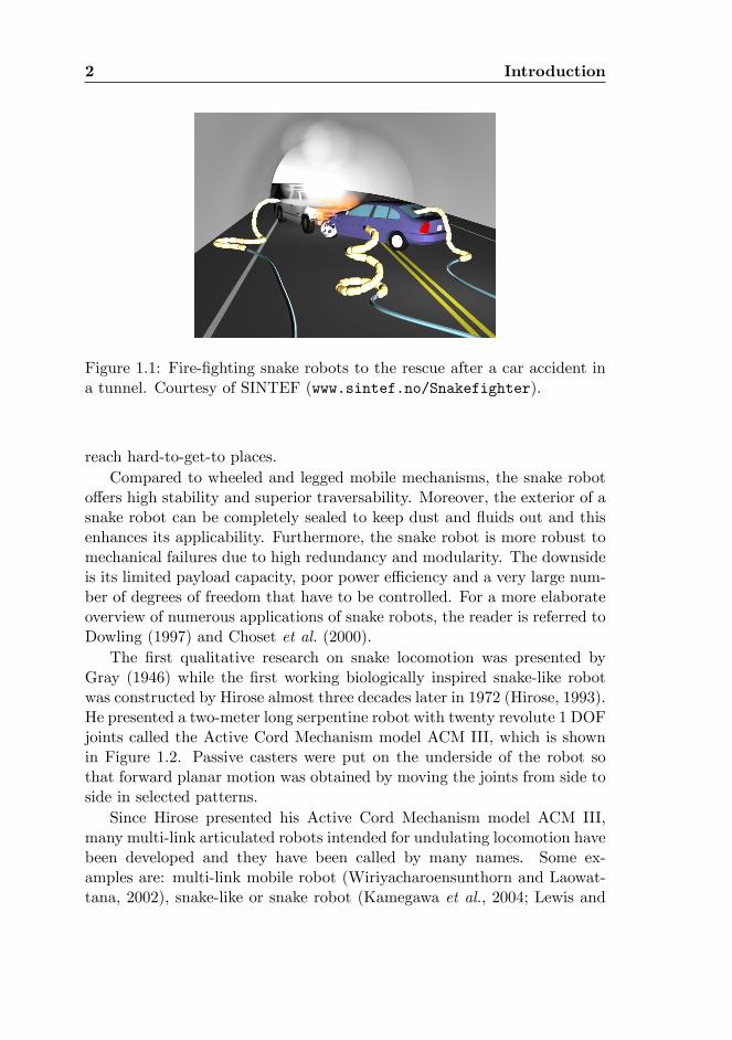
Snake robots may one day play a crucial role in search and rescue op-erations, �re-�ghting and inspection and maintenance. The highly artic-ulated body allows the snake robot to traverse di¢ cult terrains such ascollapsed buildings or the chaotic environment caused by a car collision ina tunnel as visualized in Figure 1.1. The snake robot could move withindestroyed buildings looking for people while simultaneously bringing com-munication equipment together with small amounts of food and water toanyone trapped by the shattered building. A rescue operation involving asnake robot is envisioned in Miller (2002). Moreover, the snake robot canbe used for inspection and maintenance of complex and possibly hazardousareas of industrial plants such as nuclear facilities. In a city it could inspectthe sewer system looking for leaks or aid �re-�ghters. Also, snake robotswith one end �xed to a base may be used as robot manipulators that can
2 Introduction
Figure 1.1: Fire-�ghting snake robots to the rescue after a car accident ina tunnel. Courtesy of SINTEF (www.sintef.no/Snakefighter).
reach hard-to-get-to places.Compared to wheeled and legged mobile mechanisms, the snake robot
o¤ers high stability and superior traversability. Moreover, the exterior of asnake robot can be completely sealed to keep dust and �uids out and thisenhances its applicability. Furthermore, the snake robot is more robust tomechanical failures due to high redundancy and modularity. The downsideis its limited payload capacity, poor power e¢ ciency and a very large num-ber of degrees of freedom that have to be controlled. For a more elaborateoverview of numerous applications of snake robots, the reader is referred toDowling (1997) and Choset et al. (2000).
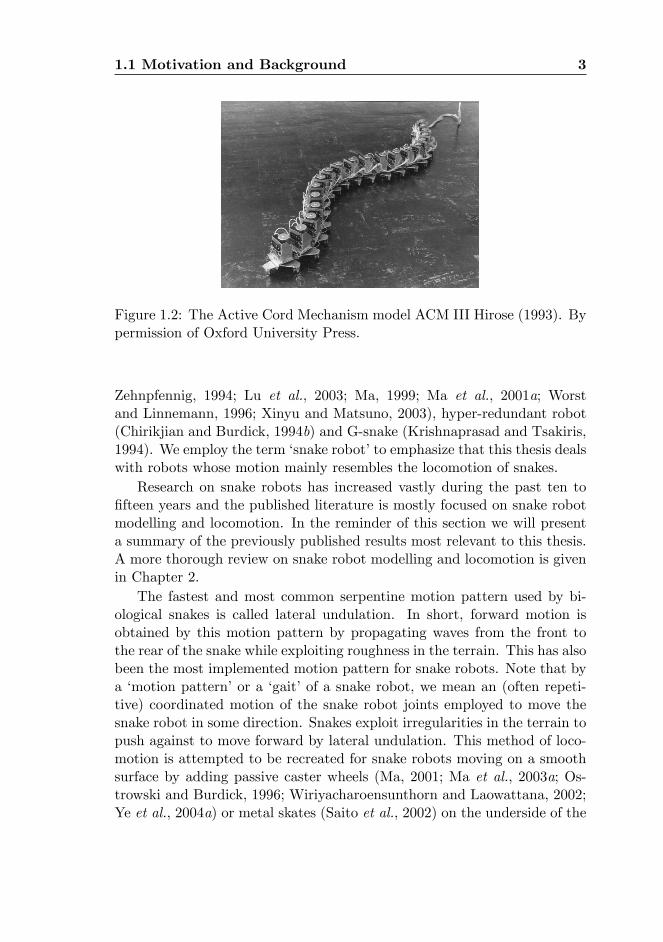
The �rst qualitative research on snake locomotion was presented byGray (1946) while the �rst working biologically inspired snake-like robotwas constructed by Hirose almost three decades later in 1972 (Hirose, 1993).He presented a two-meter long serpentine robot with twenty revolute 1 DOFjoints called the Active Cord Mechanism model ACM III, which is shownin Figure 1.2. Passive casters were put on the underside of the robot sothat forward planar motion was obtained by moving the joints from side toside in selected patterns.
Since Hirose presented his Active Cord Mechanism model ACM III,many multi-link articulated robots intended for undulating locomotion havebeen developed and they have been called by many names. Some ex-amples are: multi-link mobile robot (Wiriyacharoensunthorn and Laowat-tana, 2002), snake-like or snake robot (Kamegawa et al., 2004; Lewis and
1.1 Motivation and Background 3
Figure 1.2: The Active Cord Mechanism model ACM III Hirose (1993). Bypermission of Oxford University Press.
Zehnpfennig, 1994; Lu et al., 2003; Ma, 1999; Ma et al., 2001a; Worstand Linnemann, 1996; Xinyu and Matsuno, 2003), hyper-redundant robot(Chirikjian and Burdick, 1994b) and G-snake (Krishnaprasad and Tsakiris,1994). We employ the term �snake robot�to emphasize that this thesis dealswith robots whose motion mainly resembles the locomotion of snakes.
Research on snake robots has increased vastly during the past ten to�fteen years and the published literature is mostly focused on snake robotmodelling and locomotion. In the reminder of this section we will presenta summary of the previously published results most relevant to this thesis.A more thorough review on snake robot modelling and locomotion is givenin Chapter 2.
The fastest and most common serpentine motion pattern used by bi-ological snakes is called lateral undulation. In short, forward motion isobtained by this motion pattern by propagating waves from the front tothe rear of the snake while exploiting roughness in the terrain. This has alsobeen the most implemented motion pattern for snake robots. Note that bya �motion pattern�or a �gait�of a snake robot, we mean an (often repeti-tive) coordinated motion of the snake robot joints employed to move thesnake robot in some direction. Snakes exploit irregularities in the terrain topush against to move forward by lateral undulation. This method of loco-motion is attempted to be recreated for snake robots moving on a smoothsurface by adding passive caster wheels (Ma, 2001; Ma et al., 2003a; Os-trowski and Burdick, 1996; Wiriyacharoensunthorn and Laowattana, 2002;Ye et al., 2004a) or metal skates (Saito et al., 2002) on the underside of the
4 Introduction
snake robot body. Relatively fast locomotion is obtained for snake robotswith caster wheels travelling on a solid smooth surface. The dependencyon the surface is important since the friction property of the snake robotlinks must be such that the links slide easier forward and backward thansideways for e¢ cient snake robot locomotion by lateral undulation.
The dependency on the ground surface can be relaxed by mimickingbiological snakes and utilizing external objects to move forward. This isthe motivation for developing snake robots that exploit obstacles for loco-motion. We de�ne obstacle aided locomotion as the snake robot locomotionwhere the snake robot utilizes walls or other external objects, apart fromthe �at ground, for propulsion. Obstacle aided locomotion for snake robotswas �rst investigated by Hirose in 1976 and experiments with a snake robotwith passive caster wheels moving through a winding track were presentedin Hirose and Umetani (1976) and Hirose (1993). More recently, Bayrak-taroglu and Blazevic (2005) and Bayraktaroglu et al. (2006) elaboratedon obstacle aided locomotion for wheel-less snake robots. The dynamicsof such locomotion was simulated with the dynamic simulation softwareWorkingModelr in Bayraktaroglu and Blazevic (2005), where the rigidbody contact (i.e. the contact between an obstacle and the snake robot) isrepresented by a spring-damper model (i.e. a compliant contact model).
Snake robots capable of 3D motion appeared more recently(Chirikjian and Burdick, 1993, 1995; Hirose and Morishima, 1990; Lilje-bäck et al., 2005; Mori and Hirose, 2002) and, together with the robots,mathematical models of both the kinematics and the dynamics of snakerobots were also developed. Purely kinematic 3D models were presented inBurdick et al. (1993), Chirikjian and Burdick (1995) and Ma et al. (2003b).In such models, friction is not considered in the contact between the snakerobot and the ground surface. Instead, it is assumed in Ma et al. (2003b)that a snake robot link can slide without friction forward and backward.This can be achieved by adding passive caster wheels, which introducesnon-holonomic constraints, to the underside of the snake robot. A di¤erentapproach presented in Burdick et al. (1993) and Chirikjian and Burdick(1995) is to assume that the parts of the snake robot in contact with theground are anchored to the ground surface. Then the other parts of thesnake robot body may move without being subjected to friction forces.
A model of the motion dynamics is needed to describe the friction forcesa snake robot is subjected to when moving over a surface. Most mathemat-ical models that describe the dynamics of snake robot motion are limited toplanar (2D) motion (Ma, 2001; Ma et al., 2003a; McIsaac and Ostrowski,
1.1 Motivation and Background 5
2003b; Saito et al., 2002) while 3D models of snake robots have only recentlybeen developed (Liljebäck et al., 2005; Ma et al., 2004) where the contactbetween a snake robot and the ground surface is modelled as compliant.3D models facilitate testing and development of 3D serpentine motion pat-terns such as sinus-lifting (similar to lateral undulation, but with an addi-tional vertical wave) and sidewinding (a gait commonly employed by desertsnakes). There exists various software to model and simulate dynamicalsystems. 3D simulations of a snake robot are presented in Dowling (1999,1997) where such software is employed to de�ne and simulate a 3D snakerobot. However, details of this implementation are not presented and thesimulations are thus not easily reproducible by the reader.
On a �at surface the ability of a snake robot to move forward is de-pendent on the friction between the ground surface and the body of thesnake robot. Hence, the friction forces and the unilateral (upward) con-tact forces (which give rise to the friction forces) are important parts ofthe mathematical model of a snake robot. The friction forces are usuallybased on a Coulomb or viscous-like friction model (McIsaac and Ostrowski,2003b; Saito et al., 2002), and the Coulomb friction is most often modelledusing the sign-function (Ma et al., 2004; Saito et al., 2002). The unilateralcontact forces as a result of contact with the ground surface are modelledas a spring-damper system in Liljebäck et al. (2005), where the centre ofgravity of each link is employed as the contact point.
We have focused mostly on modelling in the above review, and we nowproceed to give a short comment on snake robot locomotion. Many authorsbase the choice and implementation of the most common serpentine motionpattern called lateral undulation on the serpenoid curve found in Hirose(1993). This is a curve that describes the motion of a biological snake whilemoving by lateral undulation. A snake robot can follow an approximation tothis curve by setting its joint angles according to a sine-curve that is phase-shifted between adjacent joints. This approach to snake robot locomotion iswidely implemented for snake robots that have either wheels (Ostrowski andBurdick, 1996; Prautsch and Mita, 1999) or a friction property such thateach link of the snake robot glides easier forward and backward compared totransversal motion (Ma, 2001; Saito et al., 2002). A no-slip constraint (i.e.a non-holonomic velocity constraint) on each wheel is sometimes introducedin the mathematical model and this results in that the snake robot linkscannot slip sideways. Such an approach is presented in Prautsch and Mita(1999), where the no-slip constraint allows one to signi�cantly reduce themodel. A Lyapunov-based proof for this reduced model together with a
6 Introduction
proposed controller shows that the snake robot is able to move to a positionreference. A velocity controller for a wheel-less snake robot with the frictionproperty described above is presented in Saito et al. (2002). The simulationand experimental results presented in that paper indicate that the snakerobot is able to stay within a reasonable o¤set of a desired speed. Results oncontrollability based on a kinematic description of snake robot locomotionare presented in Kelly and Murray (1995) and Ma et al. (2003b).
From the review above we see that very interesting and useful resultsare published on snake robot modelling and locomotion. There are manyimportant aspects to consider when modelling a snake robot. The frictionmodel has to describe the frictional contact with the ground properly. More-over, a model to describe a varying normal contact force with the groundsurface is needed to simulate some motion patterns. Other approaches tosnake robot locomotion rely on having objects to push against to moveforward and in this case the contact forces between the snake robot andthe obstacles have to be de�ned in some way. In addition, we need to de-�ne some sort of exoskeleton for the snake robot for contact with obstaclesand the ground surface. In order to develop the previously published re-sult on modelling of snake robots further, we note that only unidirectionalCoulomb friction can be described by a sign-function since the direction ofthe friction force due to a snake robot link sliding on the ground surfacewill not point in the correct direction relative to the direction of the slidingvelocity for spatial friction. Moreover, a sign-function with the commonlyemployed de�nition sign (0) = 0 (i.e. not set-valued) will not give a non-zero friction force for zero sliding velocity. However, such a non-zero frictionforce is sometimes acting on rigid bodies in the stick-phase of Coulomb fric-tion. Hence, a snake robot on a slightly inclined surface will slowly slidedownward even though it should stick to the surface due to the Coulombfriction. This is because the friction force becomes zero every time the ve-locity becomes zero. Hence, the above mentioned properties of Coulombfriction cannot be modelled with the previously published friction models.Furthermore, a very high spring coe¢ cient is needed to model a hard obsta-cle (or ground surface) with a compliant contact model (which is employedin the previously published literature) and this leads to sti¤ di¤erentialequations which in turn are cumbersome to solve numerically. Moreover,it is not clear how to determine the dissipation parameters of the contactunambiguously when using a compliant model (Brogliato, 1999). Hence,there is a need for a alternative approach to describe Coulomb friction withan accurate stick-phase, and normal contact forces due to impacts with the
1.2 Main Contributions of this Thesis 7
obstacles and the ground surface with a non-compliant model.In addition, for 3D models of the dynamics of snake robots presented
in such a way that the model is possible to re-create by the reader, onlyone point on each link (most often the centre of gravity) is considered asthe contact point with the ground. Hence, rotational motion around thelongitudinal axis of a snake robot link of such a point does not result inany translational motion since the point do not have a circumference. Thismakes the models unable to perform rolling gaits such as lateral rolling.Hence, there is a need for a well-described model of a snake robot with somesort of exoskeleton (instead of just a single stationary point) for contact withthe ground surface.
For wheel-less snake robots it is not su¢ cient to consider a purely kine-matic model for the motion pattern lateral undulation, as the friction be-tween the snake robot and the ground surface is essential for locomotion.Therefore, the friction needs to be considered for wheel-less snake robotsand this motivates including the dynamics in the development of model-based controllers for snake robots. Some controllers are developed for po-sition control of a single link or a small selection of snake robot links.Moreover, controllers are proposed for velocity and heading control of asnake robot. However, for delicate operations such as inspection and main-tenance in industrial plants, every point on the snake robot body need tobe accurately controlled so that the snake robot do not unintentionally col-lide with objects on its path. Such operations require precise control of thesnake robot joints and this can be realized through a model-based design.However, no such controller is found in the previously published literature.
1.2 Main Contributions of this Thesis
This thesis �rst presents a thorough review of snake robot modelling andlocomotion. Then various mathematical models of a snake robot, togetherwith a model-based control law are developed. Furthermore, we presentsimulation results of a number of motion patterns and some of these resultsare experimentally validated.
Review: During the last ten to �fteen years, the published literature onsnake robots has increased vastly. This thesis gives an elaborateoverview and comparison of the various mathematical models andlocomotion principles for snake robots presented during this period.Both purely kinematic models and models including dynamics areinvestigated. Moreover, we provide an introduction to the source of
8 Introduction
inspiration of snake robots: biologically inspired crawling locomotion.Furthermore, di¤erent approaches to both biologically inspired loco-motion and arti�cially generated motion patterns for snake robots arediscussed.
2D model: Propulsion by some sort of obstacle aided locomotion enablesthe snake robot to move forward in rough terrain. To this end, wepresent a novel non-smooth (hybrid) mathematical model for planarwheel-less snake robots that allows a snake robot to push againstexternal obstacles apart from the �at ground. The framework of non-smooth dynamics and convex analysis allows us to systematically andaccurately incorporate both unilateral contact forces (from the ob-stacles) and friction forces based on Coulomb�s law using set-valuedforce laws. Hence, stick-slip transitions with the ground and impactswith the obstacles are modelled as instantaneous transitions. More-over, the set-valued force law results in an accurate description of theCoulomb friction which is important for snake robot locomotion on aplanar surface. Conventional numerical solvers can not be employeddirectly for numerical integration of this model due to the set-valuedforce laws and possible instantaneous velocity changes. Therefore, weshow how to implement the model for numerical treatment with anumerical integrator called the time-stepping method. Even thoughwe model the snake robot as a hybrid system, in this framework weavoid explicit switching between system equations (for example whena collision occurs). The description of the model and the method fornumerical integration are presented in such a way that people whoare new to the �eld of non-smooth dynamics can use this thesis and,in particular, Chapter 3 as an introduction to non-smooth modellingof robot manipulators with impacts and friction.
3D model: Many snake robot motion patterns require that the snake ro-bot is able to perform more than just planar motion. Therefore, the2D model is extended to a non-smooth 3D mathematical model ofa snake robot (without wheels) where a particular choice of coordi-nates results in an e¤ective way of writing the system equations. Thesame framework of non-smooth dynamics and convex analysis as infor the 2D model is employed for the 3D model. Hence, no explicitchanges between equations are necessary when collisions occur. Thisis particularly advantageous for 3D motion since the snake robot linksrepeatedly collide with the ground surface during, for example, loco-
1.2 Main Contributions of this Thesis 9
motion by sidewinding. Moreover, the set-valued force law employedto model the normal contact between the snake robot and the groundsurface and obstacles is a bene�cial alternative to the compliant (e.g.spring-damper) model employed in previously published works. Wede�ne for each link a cylindrical exoskeleton for contact with theground surface and the external obstacles. Hence, a rolling motionwill result in a sideways motion which would not be the case if onlythe centre of gravity is employed for contact with the environment.This enables us to simulate motion patterns such as lateral rolling.
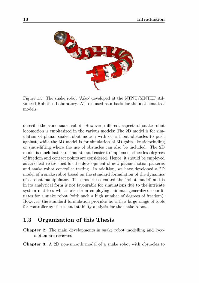
Validation of models with experimental results: Both the 2D andthe 3D mathematical model are veri�ed through experiments. Inparticular, a back-to-back comparison between numerical simulationsand experimental results is presented. Such a quantitative compar-ison is not found in any of the previously published works on snakerobots. The simulations show that the numerical treatment of bothmodels can handle both impacts with the �oor and obstacles. Theexperiments are performed with the snake robot �Aiko�depicted inFigure 1.3, which is a wheel-less snake robot with cylindrical links.Aiko has been developed at the NTNU/SINTEF Advanced RoboticsLaboratory in Trondheim, Norway.
A �robot model�and model-based control design: To be able to em-ploy the model-based control techniques developed for robot manip-ulators, we employ the standard dynamics of a robot manipulator(found in, e.g., Spong and Vidyasagar (1989)) and develop a processplant model based on this framework for a planar snake robot. Such arepresentation is not favourable for simulation due to the high numberof degrees of freedom of a snake robot so the 2D model mentioned ear-lier is still important for developing and testing new motion patterns.We employ one group of the techniques available for the robot manip-ulator model, called input-output linearization to develop a controllerfor tracking control of the snake robot joints. In order to make thestability analysis manageable, we develop a control plant model fromthe process plant model where the global orientation of the snakerobot is removed from the model. This allows us to complete a for-mal Lyapunov-based proof which shows that the joint angles convergeexponentially to their desired trajectory.
From the list of contributions given above, we see that several math-ematical models of snake robots are presented in this thesis. All models
10 Introduction
Figure 1.3: The snake robot �Aiko�developed at the NTNU/SINTEF Ad-vanced Robotics Laboratory. Aiko is used as a basis for the mathematicalmodels.
describe the same snake robot. However, di¤erent aspects of snake robotlocomotion is emphasized in the various models: The 2D model is for sim-ulation of planar snake robot motion with or without obstacles to pushagainst, while the 3D model is for simulation of 3D gaits like sidewindingor sinus-lifting where the use of obstacles can also be included. The 2Dmodel is much faster to simulate and easier to implement since less degreesof freedom and contact points are considered. Hence, it should be employedas an e¤ective test bed for the development of new planar motion patternsand snake robot controller testing. In addition, we have developed a 2Dmodel of a snake robot based on the standard formulation of the dynamicsof a robot manipulator. This model is denoted the �robot model�and isin its analytical form is not favourable for simulations due to the intricatesystem matrices which arise from employing minimal generalized coordi-nates for a snake robot (with such a high number of degrees of freedom).However, the standard formulation provides us with a large range of toolsfor controller synthesis and stability analysis for the snake robot.
1.3 Organization of this Thesis
Chapter 2: The main developments in snake robot modelling and loco-motion are reviewed.
Chapter 3: A 2D non-smooth model of a snake robot with obstacles to
1.3 Organization of this Thesis 11
push against is developed. The model is based on the framework ofnon-smooth dynamics and convex analysis. Instead of presenting thebackground theory in a separate chapter, we use the 2D model of asnake robot as an example and present the necessary theory when itis appropriate throughout this chapter.
Chapter 4: A 3D non-smooth model of a snake robot with obstacles topush against is developed. Those familiar with non-smooth dynamicsand convex analysis can read this chapter independently from Chap-ter 3.
Chapter 5: The concept of obstacle aided locomotion for snake robots iselaborated on, and we provide an overview of how a biological snakemoves by pushing against irregularities in the ground.
Chapter 6: A planar model of a snake robot based on the standard for-mulation of the dynamics of a robot manipulator is developed. More-over, an input-output linearizing controller for asymptotic trackingfor snake robot joints is designed and a formal stability proof is pro-vided.
Chapter 7: Simulation results are given for all models. In addition, back-to-back comparisons between experimental results and simulation re-sults with the 2D and 3D model are presented for a selection of ser-pentine motion patterns.
Chapter 8: Conclusions and suggestions to further work are presented.
Appendix A: An additional proof and a theorem employed in Chapter 6are described.
12 Introduction
Chapter 2
Developments in SnakeRobot Modelling andLocomotion
2.1 Introduction
During the last ten to �fteen years, the published literature on snake robotshas increased vastly and the purpose of this chapter is to provide an elabo-rate survey of the various mathematical models and locomotion principlesof snake robots presented during this period. Both purely kinematic modelsand models including dynamics are investigated. Moreover, di¤erent ap-proaches to both biologically inspired locomotion and arti�cially generatedmotion patterns for snake robots are discussed. We also provide an intro-duction to the source of inspiration for snake robot locomotion: serpentineand crawling locomotion of biological creatures. The speci�c choices ofhardware for e.g. sensors and actuators for snake robots are beyond thescope of this chapter and will not be discussed. In addition, we do not con-sider snake robots with active wheels in this thesis. For more informationon such snake robots see, for example, Kamegawa et al. (2004), Yamadaand Hirose (2006a) and Masayuki et al. (2004).
Note that the notation in this chapter sometimes di¤ers from the restof this thesis. This is because in this chapter we strive to employ the samenotation as used in the papers we discuss to ease the transition for thosewho want to explore these source papers further. However, we balancebetween using the exact same notation as in the various original papersand using a common notation for this chapter, so the correspondence is not
14 Developments in Snake Robot Modelling and Locomotion
always one-to-one.This chapter is based on Transeth and Pettersen (2006) and Transeth
and Pettersen (2008) and it is arranged as follows: Section 2.2 gives a shortintroduction to snakes and serpentine and crawling locomotion of biologicalcreatures. Various mathematical models of snake robots are presented inSection 2.3. Section 2.4 provides an overview of numerous motion patternsimplemented on snake robots, while the survey presented in this chapter isdiscussed and summarized in Section 2.5.
2.2 Biological Snakes and Inchworms
Biological snakes, inchworms and caterpillars are the source of inspirationfor most of the robots dealt with in this chapter. We will therefore start witha short introduction to snake physiology and snake locomotion. In addition,inchworm and caterpillar motion patterns are outlined. Unless otherwisespeci�ed, the contents in this section are based on Mattison (2002), Bauchot(1994) and Dowling (1997).
2.2.1 Snake Skeleton
The skeleton of a snake often consists of at least 130 vertebrae and canexceed 400 vertebrae. The range of movement between each joint is limitedto between 10 and 20 degrees for rotation from side to side and to a fewdegrees of rotation when moving up and down. A large total curvature ofthe snake body is still possible because of the high number of vertebrae.
A very small rotation is also possible around the direction along thesnake body. This property is employed when the snake moves sideways bysidewinding.
2.2.2 Snake Skin
Since snakes have no legs, the skin surface plays an important role in snakelocomotion (Bauchot, 1994). The snake should experience little frictionwhen sliding forward, but great friction when pushed backward. The skin isusually covered with scales with tiny indentations which facilitate forwardlocomotion. The scales form an edge to the belly during motion whichresults in that the friction between the underside of the snake and theground is higher transversal to the snake body than along it (Hirose, 1993).
2.2 Biological Snakes and Inchworms 15
2.2.3 Locomotion � The Source of Inspiration for SnakeRobots
Most motion patterns implemented for snake robots are inspired by loco-motion of snakes. However, inchworms and caterpillars are also used asinspiration. The relevant motion patterns of all these creatures will beoutlined in the following.
Lateral Undulation
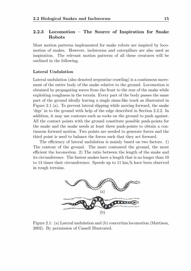
Lateral undulation (also denoted serpentine crawling) is a continuous move-ment of the entire body of the snake relative to the ground. Locomotion isobtained by propagating waves from the front to the rear of the snake whileexploiting roughness in the terrain. Every part of the body passes the samepart of the ground ideally leaving a single sinus-like track as illustrated inFigure 2.1 (a). To prevent lateral slipping while moving forward, the snake�digs�in to the ground with help of the edge described in Section 2.2.2. Inaddition, it may use contours such as rocks on the ground to push against.All the contact points with the ground constitute possible push-points forthe snake and the snake needs at least three push-points to obtain a con-tinuous forward motion. Two points are needed to generate forces and thethird point is used to balance the forces such that they act forward.
The e¢ ciency of lateral undulation is mainly based on two factors. 1)The contour of the ground. The more contoured the ground, the moree¢ cient the locomotion. 2) The ratio between the length of the snake andits circumference. The fastest snakes have a length that is no longer than 10to 13 times their circumference. Speeds up to 11 km/h have been observedin rough terrains.
Figure 2.1: (a) Lateral undulation and (b) concertina locomotion (Mattison,2002). By permission of Cassell Illustrated.
16 Developments in Snake Robot Modelling and Locomotion
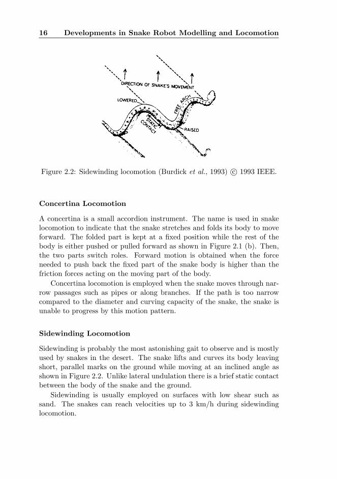
Figure 2.2: Sidewinding locomotion (Burdick et al., 1993) c 1993 IEEE.
Concertina Locomotion
A concertina is a small accordion instrument. The name is used in snakelocomotion to indicate that the snake stretches and folds its body to moveforward. The folded part is kept at a �xed position while the rest of thebody is either pushed or pulled forward as shown in Figure 2.1 (b). Then,the two parts switch roles. Forward motion is obtained when the forceneeded to push back the �xed part of the snake body is higher than thefriction forces acting on the moving part of the body.
Concertina locomotion is employed when the snake moves through nar-row passages such as pipes or along branches. If the path is too narrowcompared to the diameter and curving capacity of the snake, the snake isunable to progress by this motion pattern.
Sidewinding Locomotion
Sidewinding is probably the most astonishing gait to observe and is mostlyused by snakes in the desert. The snake lifts and curves its body leavingshort, parallel marks on the ground while moving at an inclined angle asshown in Figure 2.2. Unlike lateral undulation there is a brief static contactbetween the body of the snake and the ground.
Sidewinding is usually employed on surfaces with low shear such assand. The snakes can reach velocities up to 3 km/h during sidewindinglocomotion.
2.3 Design and Mathematical Modelling 17
Other Snake Gaits
Snakes also have gaits that are employed in special situations or by certainspecies. These are e.g. rectilinear crawling, burrowing, jumping, sinus-lifting, skidding, swimming and climbing. The latter four, which are ormay be used for snake robots, are described as follows.
Sinus-lifting is a modi�cation of lateral undulation where parts of thetrunk are lifted to avoid lateral slippage and to optimise propulsive force(Hirose, 1993). This gait is employed for high speeds.
A variation of lateral undulation is called skidding (also denoted slide-pushing) and is employed when moving past low-friction surfaces. Thesnake rests its head on the ground and then sends a �exion wave downthrough its body. This is repeated in a zigzag pattern and is a very energy-ine¢ cient way of locomotion.
Almost all snakes can swim. They move forward by undulating laterallylike an eel.
Long and thin bodied snakes can climb trees by vertical lateral undu-lation. Parts of their body hang freely in the air, while branches are usedas support.
Inchworm and Caterpillar Locomotion
An inchworm moves forward by grabbing the ground with its front legswhile the rear end is pulled forward. The rear legs then grab the groundand the inchworm lifts its front legs and straightens its body. Caterpillarssend a vertical travelling wave through their body from the end to the frontin order to move forward. Small legs give the necessary friction force whileon the ground.
2.3 Design and Mathematical Modelling
The mathematical model of a snake robot, of course, depends on its design.To categorize the di¤erent snake robot designs we recognize certain basicproperties: 1) Type of joints, 2) number of degrees of freedom (DOF) and3) with or without passive caster wheels. Most snake robots consist of linksconnected by revolute joints with one or two DOF. On some robots, thelinks are extensible (i.e. prismatic joints). To achieve the desired frictionalproperty for lateral undulation mentioned in Section 2.2, some snake robotsare equipped with passive wheels. When wheels are employed, the dynamicsof the interaction between the robot and the ground surface is often ignored.
18 Developments in Snake Robot Modelling and Locomotion
If no wheels are attached, this friction force needs to be considered for some,but not all, gaits (see Section 2.4).
In the following, the mathematical modelling of the di¤erent snake ro-bots is divided into kinematics and dynamics.
2.3.1 Kinematics
The kinematics describes the geometrical aspect of motion. Di¤erent mod-elling techniques ranging from classical methods such as the Denavit-Hartenberg (D-H) convention (see e.g. Murray et al. (1994) for more onthe D-H convention) to specialized methods for hyper-redundant structures(structures with a high number of DOF) have been employed. The followingsubsections will elaborate on the di¤erent modelling techniques.
The Denavit-Hartenberg Convention
The Denavit-Hartenberg convention is a well established method for de-scribing the position and orientation of the links of a robot manipulatorwith respect to a (usually �xed) base frame. Di¤erent solutions are pre-sented to deal with the fact that the base is not �xed on a snake robot(Liljebäck et al., 2005; Poi et al., 1998).
Poi et al. (1998) present a snake robot that is made of 9 equal modules.Each module consists of seven revolute 1 DOF joints which are connectedby links of equal length. Three joints and four joints have the axis of ro-tation perpendicular to the horizontal and vertical plane, respectively, andthe joints are placed alternately. Each module is parameterised with theD-H convention. A modi�cation to the convention has been proposed byplacing the base coordinate system on the closest motionless link to the partof structure which is in motion. Hence, the links in motion are describedin an inertial frame. The snake robot described in Poi et al. (1998) movesonly four or �ve modules simultaneously, so giving the position and orienta-tion relative to the closest motionless link prevents traversing through thecomplete structure to obtain positions and orientations in an inertial frame(such traversing is usually necessary when employing the D-H conventionsince we are dealing with minimal coordinates).
The motion patterns employed in Liljebäck et al. (2005), sidewindingand lateral undulation, are based on constant joint movement so we haveto traverse through the whole structure to obtain the inertial position andorientation of each snake robot link, and hence the previously presentedapproach (Poi et al., 1998) will not simplify the mathematical structure.
2.3 Design and Mathematical Modelling 19
Therefore, a virtual structure for orientation and position (VSOP) is intro-duced to be able to describe the kinematics of the snake robot in an inertialreference frame. Liljebäck et al. (2005) present a snake robot with 5 revo-lute 2 DOF joints. The VSOP describes the position and orientation of therearmost link of the snake robot relative to an inertial reference frame by 3orthogonal prismatic joints and 3 orthogonal revolute joints, respectively.These virtual joints are connected by links with no mass. By employing theVSOP in the Denavit-Hartenberg convention, the position and orientationof each joint is given in an inertial coordinate system.
A Backbone Curve
Instead of starting by �nding the position and orientation of each joint di-rectly as with the Denavit-Hartenberg convention, a curve that describesthe shape of the �spine�of the snake robot can be employed (Chirikjian,1992; Chirikjian and Burdick, 1991, 1994b; Yamada and Hirose, 2006b). TheFrenet-Serret apparatus (see Do Carmo, 1976) is employed in the classicalhandling of the geometry of curves (Chirikjian and Burdick, 1994b). How-ever, this approach has some limitations (Chirikjian and Burdick, 1994b).First, the Frenet-Serret frames assigned along the curve are not de�ned forstraight line segments. Second, the vector function describing the spatialcurve requires the numerical solution of a cumbersome di¤erential equa-tion. The introduction of backbone curves (see e.g. Chirikjian and Burdick,1994b) is a way of handling these limitations. The backbone curve is de�nedas �a piecewise continuous curve that captures the important macroscopicgeometric features of a hyper-redundant robot� (Chirikjian and Burdick,1994b) and it typically runs through the spine of the snake robot. A set oforthonormal reference frames are found along the backbone curve to specifythe actual snake robot con�guration. The backbone curve parameterisationtogether with an associated set of orthonormal reference frames is called abackbone curve reference set and allows for snake robots built from bothprismatic and revolute joints (Chirikjian and Burdick, 1991).
A recent alternative approach to the methods presented by Chirikjianand Burdick (Chirikjian and Burdick, 1991, 1994b) has been given by Ya-mada and Hirose (2006b). This approach is called the bellows model and isspeci�cally designed for distinguishing explicitly between the twisting andbending of the body of the snake robot. This is advantageous since mostsnake robots are designed with joints capable of bending, but not twisting(for example snake robots with cardan joints). Hence, the ability to twistcan simply be left out of the model of the snake robot. So far, there are no
20 Developments in Snake Robot Modelling and Locomotion
published results on how to �t the continuous bellows model to an actualsnake robot (which has a discrete morphology).
The problem of determining joint angles of a robot manipulator giventhe end-e¤ector position is called the inverse kinematics problem. Forhyper-redundant manipulators (such as snake robots) this is a very com-putationally demanding task. When the backbone curve is employed, theproblem is reduced to determining the proper time varying behaviour of thebackbone reference set and this approach has been employed for controllinga real snake robot in Chirikjian and Burdick (1994a).
The above methods described in this section are suitable for abstraction,understanding and development of the geometric aspects of snake robotmotion planning (which may initially be quite complicated due to the highnumber of DOF), in particular when the dynamics may be neglected.
Non-holonomic Constraints and Snake Robots with Passive CasterWheels
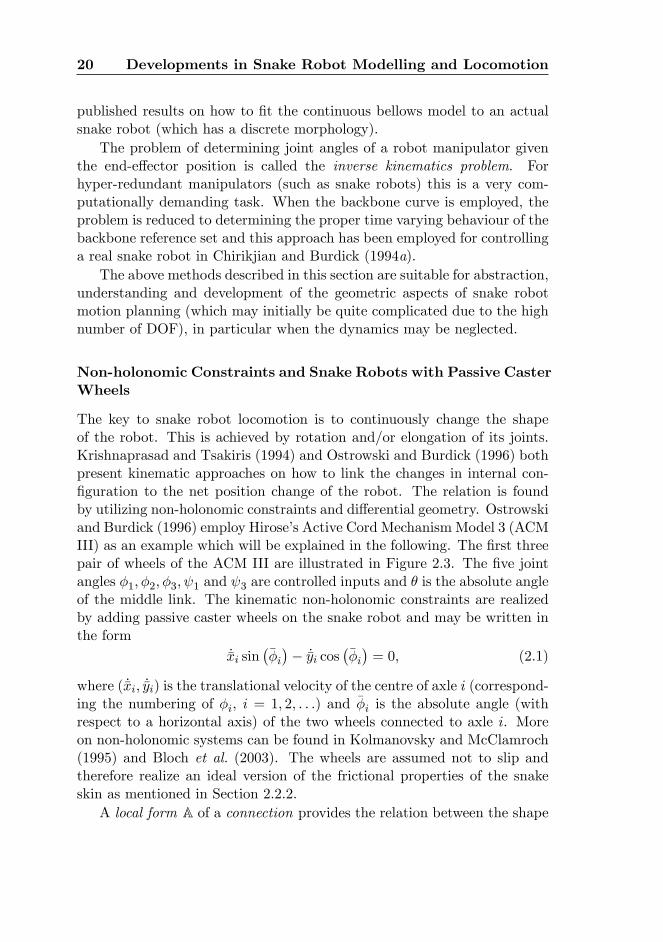
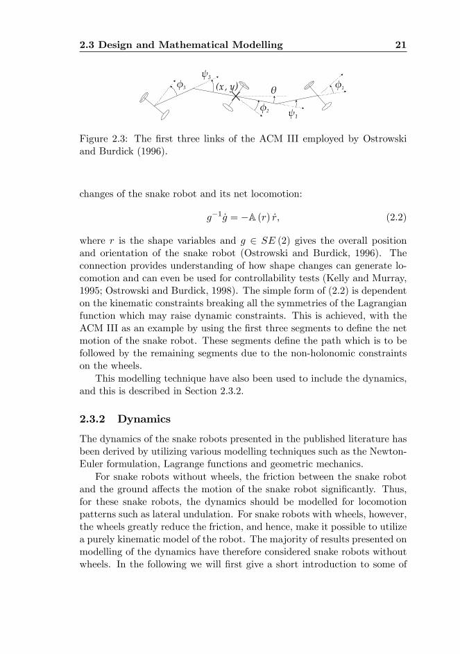
The key to snake robot locomotion is to continuously change the shapeof the robot. This is achieved by rotation and/or elongation of its joints.Krishnaprasad and Tsakiris (1994) and Ostrowski and Burdick (1996) bothpresent kinematic approaches on how to link the changes in internal con-�guration to the net position change of the robot. The relation is foundby utilizing non-holonomic constraints and di¤erential geometry. Ostrowskiand Burdick (1996) employ Hirose�s Active Cord Mechanism Model 3 (ACMIII) as an example which will be explained in the following. The �rst threepair of wheels of the ACM III are illustrated in Figure 2.3. The �ve jointangles �1; �2; �3; 1 and 3 are controlled inputs and � is the absolute angleof the middle link. The kinematic non-holonomic constraints are realizedby adding passive caster wheels on the snake robot and may be written inthe form
_�xi sin���i�� _�yi cos
���i�= 0; (2.1)
where ( _�xi; _�yi) is the translational velocity of the centre of axle i (correspond-ing the numbering of �i, i = 1; 2; : : :) and ��i is the absolute angle (withrespect to a horizontal axis) of the two wheels connected to axle i. Moreon non-holonomic systems can be found in Kolmanovsky and McClamroch(1995) and Bloch et al. (2003). The wheels are assumed not to slip andtherefore realize an ideal version of the frictional properties of the snakeskin as mentioned in Section 2.2.2.
A local form A of a connection provides the relation between the shape
2.3 Design and Mathematical Modelling 21
Figure 2.3: The �rst three links of the ACM III employed by Ostrowskiand Burdick (1996).
changes of the snake robot and its net locomotion:
g�1 _g = �A (r) _r; (2.2)
where r is the shape variables and g 2 SE (2) gives the overall positionand orientation of the snake robot (Ostrowski and Burdick, 1996). Theconnection provides understanding of how shape changes can generate lo-comotion and can even be used for controllability tests (Kelly and Murray,1995; Ostrowski and Burdick, 1998). The simple form of (2.2) is dependenton the kinematic constraints breaking all the symmetries of the Lagrangianfunction which may raise dynamic constraints. This is achieved, with theACM III as an example by using the �rst three segments to de�ne the netmotion of the snake robot. These segments de�ne the path which is to befollowed by the remaining segments due to the non-holonomic constraintson the wheels.
This modelling technique have also been used to include the dynamics,and this is described in Section 2.3.2.
2.3.2 Dynamics
The dynamics of the snake robots presented in the published literature hasbeen derived by utilizing various modelling techniques such as the Newton-Euler formulation, Lagrange functions and geometric mechanics.
For snake robots without wheels, the friction between the snake robotand the ground a¤ects the motion of the snake robot signi�cantly. Thus,for these snake robots, the dynamics should be modelled for locomotionpatterns such as lateral undulation. For snake robots with wheels, however,the wheels greatly reduce the friction, and hence, make it possible to utilizea purely kinematic model of the robot. The majority of results presented onmodelling of the dynamics have therefore considered snake robots withoutwheels. In the following we will �rst give a short introduction to some of
22 Developments in Snake Robot Modelling and Locomotion
the notation utilized below, then we give a brief overview of a selection ofthe results reported on the modelling of dynamics of wheeled snake robotsand �nally we present results on snake robots without wheels.
To ease the presentation of the mathematical models, a common no-tation for some of the material is presented, which is based in parts onPrautsch and Mita (1999) and Saito et al. (2002). Denote the mass mi,length 2li and moment of inertia Ji for each link i = 1; 2; :::; n. The snakerobot moves in the xy-plane. Denote the angle �i between link i and theinertial (base) x-axis. Denote position of the centre of gravity (CG) oflink i by (xi; yi). Denote the unit vectors tangential e
Bit 2 R2 and nor-
mal eBin 2 R2 to the link i in the horizontal xy-plane. Hence, eBit points
along link i and eBin ? eBit . Denote the velocity vi =�_xi _yi
�T 2 R2 oflink i, and tangential and normal velocity of link i vi;t = e
Bit
�eBit
�Tvi and
vi;n = eBin
�eBin�Tvi, respectively.
The friction forces that act on the CG of link i are denotedf i =
�fxi fyi
�T 2 R2 where fxi , fyi are friction forces between link iand the ground along the x- and y-direction of the inertial frame, respec-tively. The coe¢ cients of friction tangential and normal to link i are c(j)i;tand c(j)i;n, respectively, where j is used in this chapter to distinguish betweenthe coe¢ cients in the various friction models.
Snake Robots with Passive Caster Wheels
A desired property for moving by lateral undulation, is to keep the di¤erencebetween lateral and longitudinal friction as high as possible. This propertyof friction can be obtained by attaching caster wheels to the belly of thesnake robot. The equations of motion of a simpli�ed version of the ACMIII snake robot used by Hirose (1993) are presented by Prautsch and Mita(1999). The robot is the same as the ACM III shown in Figure 1.2 andFigure 2.3 except that the wheel axles are �xed. The dynamic model isderived to utilize acceleration-based control algorithms. It is assumed thatthe wheels do not slip sideways.
A snake robot (called the SR#2) has been presented and comparedto the ACM III by Wiriyacharoensunthorn and Laowattana (2002). TheActive Cord Mechanism (ACM) modelling assumes that the wheels do notslip. This non-slippage introduces non-holonomic constraints. The SR#2model is based on holonomic framework and is hence without the no-slipcondition. The argument used against assuming no slip is that it is di¢ cult
2.3 Design and Mathematical Modelling 23
to control the torques in the joints such that the assumption is satis�ed.Simulations show the ACM III build up an error in position while followinga circular path. This is not the case for SR#2, something which makes ita more accurate model for this scenario.
The above models have all described planar motion. Moreover, a 3Dmodel of the dynamics of a snake robot with wheels that do not slip hasbeen presented by Ma et al. (2004). In addition, a system equation forcontrol of the height of the wheels is given and computer simulations arepresented in that paper.
Snake Robots without Wheels
The use of wheels may decrease traversability (Saito et al., 2002), thuswheel-less robots may have an advantage. As discussed earlier, frictionplays a signi�cant role for wheel-less snake robots, hence it is necessary tomodel the dynamics and not only the kinematics for relatively high speedmotion (for certain motion patterns during low speed motion, a kinematicmodel may su¢ ce). First, we will give an overview of the friction andcontact models employed for snake robots, then a selection of dynamicmodels derived for snake robots without wheels will be presented.
Friction and Contact Models The friction models presented in lit-erature on snake robots are based on a Coulomb or viscous-like frictionmodel and such models are explained, for instance, in Egeland and Grav-dahl (2002). For 3D models of snake robots, it is necessary to model thenormal contact force due to impacts and sustained contact with the ground,in addition to the friction force. This force has been described as compliantby a spring-damper model in Liljebäck et al. (2005) as
fNi =
�0 ; zi � 0�k � zi � d � _zi ; zi < 0;
(2.3)
where zi 2 R is the height of the centre of gravity of link i, _zi = dzdt , k 2 R
+
is the constant spring coe¢ cient of the ground, and d 2 R+ is a constantdamping coe¢ cient that serves to damp out the oscillations induced by thespring. The friction force on link i, based on a simple, viscous-like model,is now written as
f i = �c(1)i;t jfNi jvi;t � c
(1)i;n jfNi jvi;n 2 R
2: (2.4)
The sum of forces acting on link i in the model presented by Liljebäck etal. (2005) is f3Di =
�fTi fNi
�T 2 R3. The spring coe¢ cient k needs to be
24 Developments in Snake Robot Modelling and Locomotion
set very high to imitate a solid surface. Hence, the total system is sti¤ andrequires a very small simulation step size to be simulated. However, theconstitutive law (2.3) for the normal force provides an intuitive and simpleapproach to implementing the normal force. A friction model includingboth static and dynamic friction properties for a 3D dynamic model isgiven by Ma et al. (2004).
The 2D anisotropic viscous friction model used by Grabec (2002) canbe derived from (2.4) by setting fNi � 1. In this case the friction force isfound from
f i = Hivi, (2.5)
where
Hi = c(2)i;n
" 1�
c(2)i;t
c(2)i;n
!eBit
�eBit
�T� I2�2
#; (2.6)
and I2�2 2 R2�2 is a unit matrix.The e¤ect of rotational motion of the links is introduced in the two 2D
friction models, one with viscous and one with Coulomb friction, presentedby Saito et al. (2002). Both models are derived by integrating the in�nites-imal friction forces on a link. The translational part of the viscous frictionmodel is given by (2.4) with fNi = mi (i.e. fNi is not an actual force). Thetotal viscous friction torque due to rotational velocity around the centre ofgravity of link i is found to be
� i = �c(3)i;nmil
2i
3_�i 2 R. (2.7)
For translational motion the friction force based on Coulomb�s law is foundfor _�i = 0 as (Saito et al., 2002)
f i = �mig
�cos �i � sin �isin �i cos �i
�"c(3)i;t 0
0 c(3)i;n
#sign
0@24�eBit �T vi�eBin�Tvi
351A : (2.8)
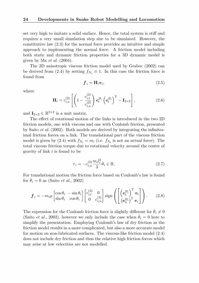
The expression for the Coulomb friction force is slightly di¤erent for _�i 6= 0(Saito et al., 2002), however we only include the case when _�i = 0 here tosimplify the presentation. Employing Coulomb�s law of dry friction as thefriction model results in a more complicated, but also a more accurate modelfor motion on non-lubricated surfaces. The viscous-like friction model (2.4)does not include dry friction and thus the relative high friction forces whichmay arise at low velocities are not modelled.
2.3 Design and Mathematical Modelling 25
For most of the gaits simulated with the above friction models, theproperty ci;t < ci;n has been implemented to realize the anisotropic frictionproperty of a snake moving by lateral undulation. It may be di¢ cult todesign a snake robot with ci;t < ci;n on a general surface. Sidewinding hasbeen implemented with an isotropic friction model (ci;n = ci;t) by Liljebäck(2004) and as a purely kinematic case by Burdick et al. (1993). Specialgaits for planar motion based on an isotropic friction model are detailed byChernousko (2005, 2000).
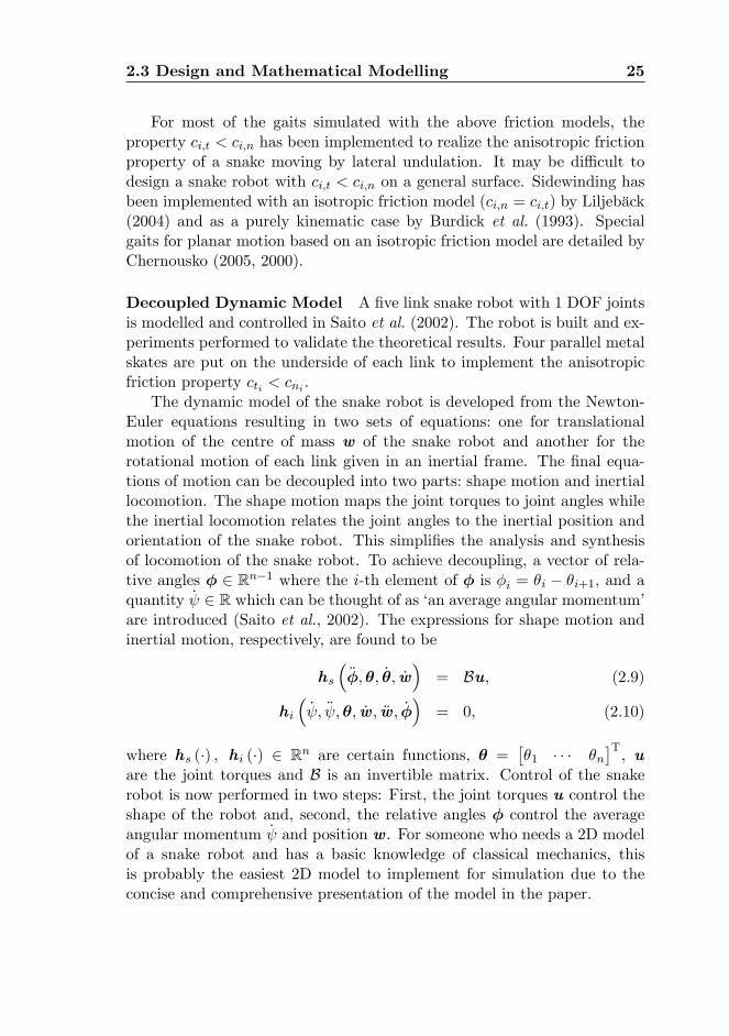
Decoupled Dynamic Model A �ve link snake robot with 1 DOF jointsis modelled and controlled in Saito et al. (2002). The robot is built and ex-periments performed to validate the theoretical results. Four parallel metalskates are put on the underside of each link to implement the anisotropicfriction property cti < cni .
The dynamic model of the snake robot is developed from the Newton-Euler equations resulting in two sets of equations: one for translationalmotion of the centre of mass w of the snake robot and another for therotational motion of each link given in an inertial frame. The �nal equa-tions of motion can be decoupled into two parts: shape motion and inertiallocomotion. The shape motion maps the joint torques to joint angles whilethe inertial locomotion relates the joint angles to the inertial position andorientation of the snake robot. This simpli�es the analysis and synthesisof locomotion of the snake robot. To achieve decoupling, a vector of rela-tive angles � 2 Rn�1 where the i-th element of � is �i = �i � �i+1, and aquantity _ 2 R which can be thought of as �an average angular momentum�are introduced (Saito et al., 2002). The expressions for shape motion andinertial motion, respectively, are found to be
hs
���;�; _�; _w
�= Bu; (2.9)
hi
�_ ; � ;�; _w; �w; _�
�= 0; (2.10)
where hs (�) ; hi (�) 2 Rn are certain functions, � =��1 � � � �n
�T, u
are the joint torques and B is an invertible matrix. Control of the snakerobot is now performed in two steps: First, the joint torques u control theshape of the robot and, second, the relative angles � control the averageangular momentum _ and position w. For someone who needs a 2D modelof a snake robot and has a basic knowledge of classical mechanics, thisis probably the easiest 2D model to implement for simulation due to theconcise and comprehensive presentation of the model in the paper.
26 Developments in Snake Robot Modelling and Locomotion
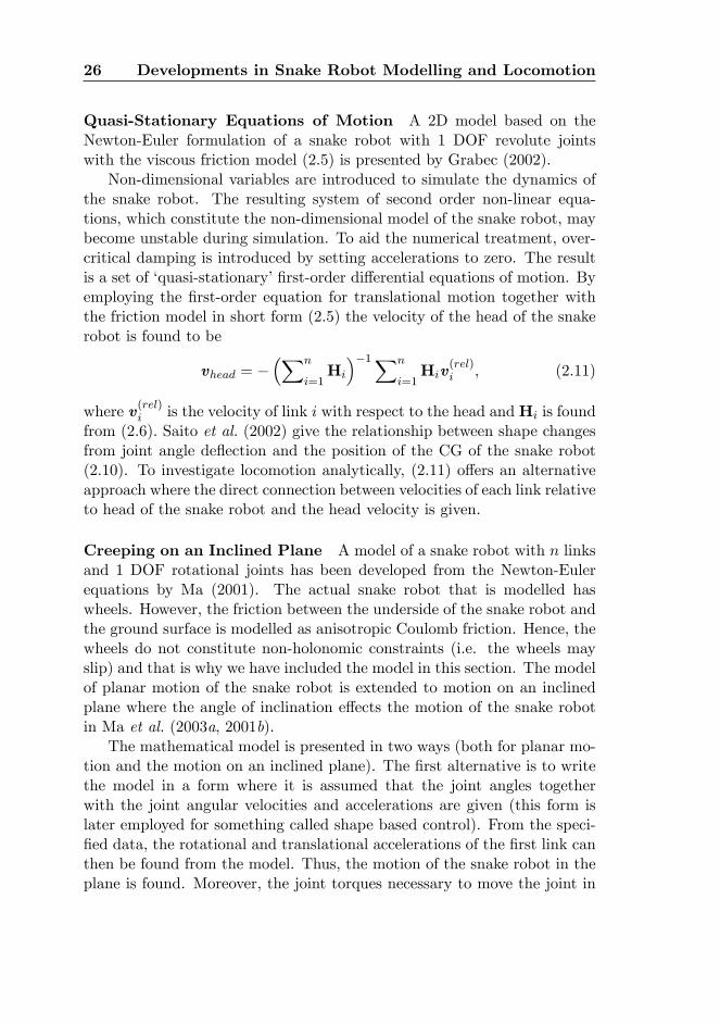
Quasi-Stationary Equations of Motion A 2D model based on theNewton-Euler formulation of a snake robot with 1 DOF revolute jointswith the viscous friction model (2.5) is presented by Grabec (2002).
Non-dimensional variables are introduced to simulate the dynamics ofthe snake robot. The resulting system of second order non-linear equa-tions, which constitute the non-dimensional model of the snake robot, maybecome unstable during simulation. To aid the numerical treatment, over-critical damping is introduced by setting accelerations to zero. The resultis a set of �quasi-stationary��rst-order di¤erential equations of motion. Byemploying the �rst-order equation for translational motion together withthe friction model in short form (2.5) the velocity of the head of the snakerobot is found to be
vhead = ��Xn
i=1Hi
��1Xn
i=1Hiv
(rel)i ; (2.11)
where v(rel)i is the velocity of link i with respect to the head andHi is foundfrom (2.6). Saito et al. (2002) give the relationship between shape changesfrom joint angle de�ection and the position of the CG of the snake robot(2.10). To investigate locomotion analytically, (2.11) o¤ers an alternativeapproach where the direct connection between velocities of each link relativeto head of the snake robot and the head velocity is given.
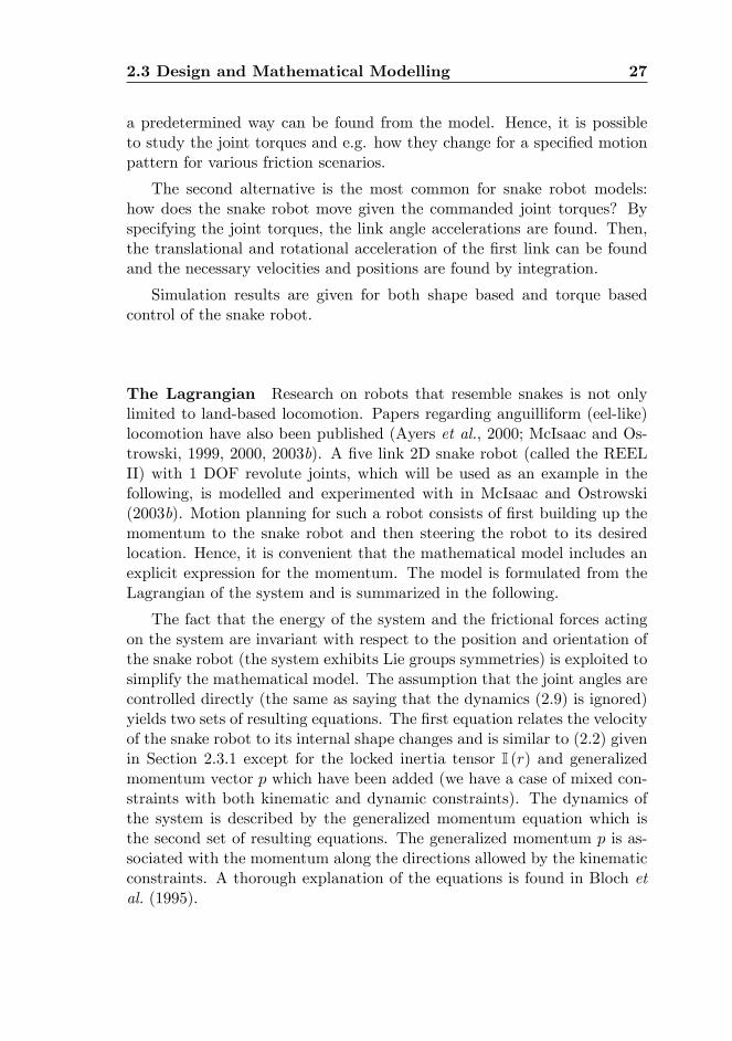
Creeping on an Inclined Plane A model of a snake robot with n linksand 1 DOF rotational joints has been developed from the Newton-Eulerequations by Ma (2001). The actual snake robot that is modelled haswheels. However, the friction between the underside of the snake robot andthe ground surface is modelled as anisotropic Coulomb friction. Hence, thewheels do not constitute non-holonomic constraints (i.e. the wheels mayslip) and that is why we have included the model in this section. The modelof planar motion of the snake robot is extended to motion on an inclinedplane where the angle of inclination e¤ects the motion of the snake robotin Ma et al. (2003a, 2001b).
The mathematical model is presented in two ways (both for planar mo-tion and the motion on an inclined plane). The �rst alternative is to writethe model in a form where it is assumed that the joint angles togetherwith the joint angular velocities and accelerations are given (this form islater employed for something called shape based control). From the speci-�ed data, the rotational and translational accelerations of the �rst link canthen be found from the model. Thus, the motion of the snake robot in theplane is found. Moreover, the joint torques necessary to move the joint in
2.3 Design and Mathematical Modelling 27
a predetermined way can be found from the model. Hence, it is possibleto study the joint torques and e.g. how they change for a speci�ed motionpattern for various friction scenarios.
The second alternative is the most common for snake robot models:how does the snake robot move given the commanded joint torques? Byspecifying the joint torques, the link angle accelerations are found. Then,the translational and rotational acceleration of the �rst link can be foundand the necessary velocities and positions are found by integration.
Simulation results are given for both shape based and torque basedcontrol of the snake robot.
The Lagrangian Research on robots that resemble snakes is not onlylimited to land-based locomotion. Papers regarding anguilliform (eel-like)locomotion have also been published (Ayers et al., 2000; McIsaac and Os-trowski, 1999, 2000, 2003b). A �ve link 2D snake robot (called the REELII) with 1 DOF revolute joints, which will be used as an example in thefollowing, is modelled and experimented with in McIsaac and Ostrowski(2003b). Motion planning for such a robot consists of �rst building up themomentum to the snake robot and then steering the robot to its desiredlocation. Hence, it is convenient that the mathematical model includes anexplicit expression for the momentum. The model is formulated from theLagrangian of the system and is summarized in the following.
The fact that the energy of the system and the frictional forces actingon the system are invariant with respect to the position and orientation ofthe snake robot (the system exhibits Lie groups symmetries) is exploited tosimplify the mathematical model. The assumption that the joint angles arecontrolled directly (the same as saying that the dynamics (2.9) is ignored)yields two sets of resulting equations. The �rst equation relates the velocityof the snake robot to its internal shape changes and is similar to (2.2) givenin Section 2.3.1 except for the locked inertia tensor I (r) and generalizedmomentum vector p which have been added (we have a case of mixed con-straints with both kinematic and dynamic constraints). The dynamics ofthe system is described by the generalized momentum equation which isthe second set of resulting equations. The generalized momentum p is as-sociated with the momentum along the directions allowed by the kinematicconstraints. A thorough explanation of the equations is found in Bloch etal. (1995).
28 Developments in Snake Robot Modelling and Locomotion
The Newton-Euler Algorithm Amathematical model of a snake robotwith �ve 2 DOF revolute joints is presented by Liljebäck et al. (2005). Asnake robot is also constructed for experiments. In addition to the actualsnake robot, a virtual structure of orientation and position (VSOP, seeSection 2.3.1) is included in the dynamic model. The VSOP together withthe snake robot have generalized minimal coordinates q 2 R2(n�1)+6 andgeneralised forces � 2 R2(n�1)+6. The Newton-Euler formulation and theVSOP perspective is employed and the dynamic model is written as
M (q) �q +C (q; _q) _q + g (q) = � + � ext; (2.12)
where M is the mass and inertia matrix, C is the Coriolis and centripetalmatrix, g (�) is the vector of gravitational forces and torques and � ext isthe vector including the external forces (friction and normal contact force).The matrices are detailed in Liljebäck (2004). The Newton-Euler algorithmhas been employed to simulate the snake robot. Hence, the full analyticalexpressions for the system matrices do not need to be found explicitly.Instead, the necessary matrices and accelerations are found numericallywith the recursive Newton-Euler algorithm. This is advantageous sincethe analytical expressions for the system matrices are extremely large fora large number of joints when minimal coordinates are employed. For amodel with non-minimal coordinates found in Ma et al. (2004), analyticalexpressions for the joint torques and head con�guration of a 3D snake robotmodel deducted from the Newton-Euler equations are shown.
The Lagrange and the Newton-Euler method are similar for rigid bodydynamics in that the expression obtained by the Lagrange method is foundby running through the Newton-Euler algorithm once. Since the Newton-Euler algorithm deals with the mathematical model as a recursive algo-rithm, it is a more e¢ cient framework for simulation than the Lagrangemethod for large models (Egeland and Gravdahl, 2002).
A modi�cation of the Newton-Euler algorithm has been presented byBoyer et al. (2006) to numerically evaluate a model of a continuous 3Dunderwater snake robot where the modelling approach is based on beamtheory.
2.4 Snake Robot Locomotion
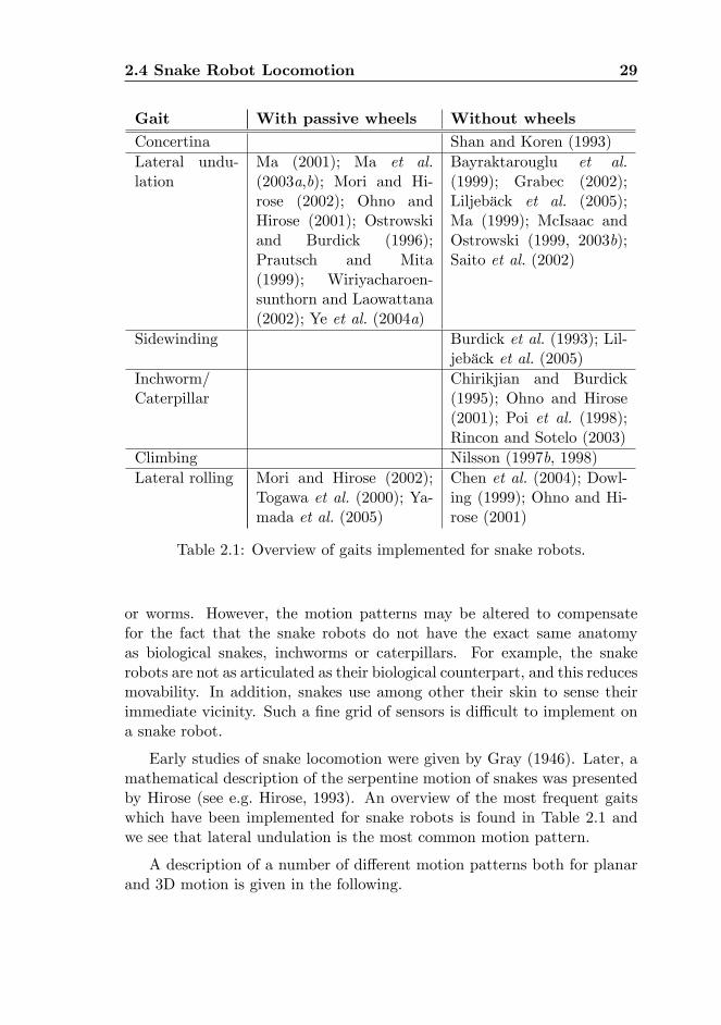
A variety of approaches on how to make a snake robot move has beenproposed. In most of the motion patterns or �gaits�used for locomotion, we�nd a distinct resemblance to the undulating locomotion of biological snakes
2.4 Snake Robot Locomotion 29
Gait With passive wheels Without wheelsConcertina Shan and Koren (1993)Lateral undu-lation
Ma (2001); Ma et al.(2003a,b); Mori and Hi-rose (2002); Ohno andHirose (2001); Ostrowskiand Burdick (1996);Prautsch and Mita(1999); Wiriyacharoen-sunthorn and Laowattana(2002); Ye et al. (2004a)
Bayraktarouglu et al.(1999); Grabec (2002);Liljebäck et al. (2005);Ma (1999); McIsaac andOstrowski (1999, 2003b);Saito et al. (2002)
Sidewinding Burdick et al. (1993); Lil-jebäck et al. (2005)
Inchworm/Caterpillar
Chirikjian and Burdick(1995); Ohno and Hirose(2001); Poi et al. (1998);Rincon and Sotelo (2003)
Climbing Nilsson (1997b, 1998)Lateral rolling Mori and Hirose (2002);
Togawa et al. (2000); Ya-mada et al. (2005)
Chen et al. (2004); Dowl-ing (1999); Ohno and Hi-rose (2001)
Table 2.1: Overview of gaits implemented for snake robots.
or worms. However, the motion patterns may be altered to compensatefor the fact that the snake robots do not have the exact same anatomyas biological snakes, inchworms or caterpillars. For example, the snakerobots are not as articulated as their biological counterpart, and this reducesmovability. In addition, snakes use among other their skin to sense theirimmediate vicinity. Such a �ne grid of sensors is di¢ cult to implement ona snake robot.
Early studies of snake locomotion were given by Gray (1946). Later, amathematical description of the serpentine motion of snakes was presentedby Hirose (see e.g. Hirose, 1993). An overview of the most frequent gaitswhich have been implemented for snake robots is found in Table 2.1 andwe see that lateral undulation is the most common motion pattern.
A description of a number of di¤erent motion patterns both for planarand 3D motion is given in the following.
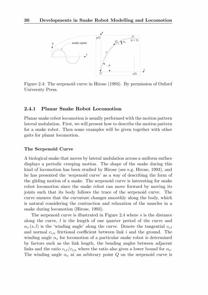
30 Developments in Snake Robot Modelling and Locomotion
Figure 2.4: The serpenoid curve in Hirose (1993). By permission of OxfordUniversity Press.
2.4.1 Planar Snake Robot Locomotion
Planar snake robot locomotion is usually performed with the motion patternlateral undulation. First, we will present how to describe the motion patternfor a snake robot. Then some examples will be given together with othergaits for planar locomotion.
The Serpenoid Curve
A biological snake that moves by lateral undulation across a uniform surfacedisplays a periodic creeping motion. The shape of the snake during thiskind of locomotion has been studied by Hirose (see e.g. Hirose, 1993), andhe has presented the �serpenoid curve�as a way of describing the form ofthe gliding motion of a snake. The serpenoid curve is interesting for snakerobot locomotion since the snake robot can move forward by moving itsjoints such that its body follows the trace of the serpenoid curve. Thecurve ensures that the curvature changes smoothly along the body, whichis natural considering the contraction and relaxation of the muscles in asnake during locomotion (Hirose, 1993).
The serpenoid curve is illustrated in Figure 2.4 where s is the distancealong the curve, l is the length of one quarter period of the curve and�s (s; l) is the �winding angle�along the curve. Denote the tangential ci;tand normal ci;n frictional coe¢ cient between link i and the ground. Thewinding angle �s for locomotion of a particular snake robot is determinedby factors such as the link length, the bending angles between adjacentlinks and the ratio ci;t=ci;n where the ratio also gives a lower bound for �s.The winding angle �s at an arbitrary point Q on the serpenoid curve is
2.4 Snake Robot Locomotion 31
found from�s (s; l) = � cos
� �2ls�, (2.13)
where � is the initial winding angle as illustrated in Figure 2.4. Unlessotherwise speci�ed, the common assumption is ci;t < ci;n which is necessaryto move forward on a �at surface by lateral undulation. However, it needsto be mentioned that a snake robot will instead move slowly backward forci;t = ci;n (Nilsson, 2004).
An alternative to the serpenoid curve has been proposed by Ma (1999)and is called the serpentine curve. Ma (1999) has shown that a snakerobot following this curve has higher locomotive e¢ ciency. For a snakerobot that does not slip, the locomotive e¢ ciency is de�ned as the ratiobetween the forces that act along the snake robot and the forces that actperpendicular to the body (Ma, 1999). The serpenoid curve is neverthelessthe most frequent employed basis for �nding the desired joint angles for asnake robot. This is probably partly due to its simplicity compared to theexpression for the serpentine curve.
Lateral Undulation for Snake Robots
The serpenoid curve cannot be exactly reproduced by a snake robot due toits discrete morphology. However, an approximation to the serpenoid curvecan be recreated by a snake robot by setting its (relative) joint referenceangle �hi;d for joints i = 1; : : : ; n� 1 as
�hi;d = Ah sin (!ht+ (i� 1)�h) + h; (2.14)
where Ah is the maximum amplitude of oscillation, �h is the phase shiftbetween adjacent links, h determines the orientation of the snake robotand !h is the angular frequency of oscillation (see e.g. Saito et al., 2002; Yeet al., 2004a). The use of h to change the heading of the snake is discussedin Ye et al. (2004a) and two alternative turning motions are also presented.The parameters !h and �h are the two most signi�cant parameters in orderto control the speed of the serpentine wave that propagates down the bodyof the snake robot.
Sideways slip should be kept as low as possible when moving by lateralundulation. This is because such slip does not contribute to forward motion.For wheel-less snake robots, sideways slip can be reduced by changing themotion pattern parameters in (2.14) according to the ratio ci;t=ci;n. Anexample on how to do this has been presented by Saito et al. (2002), wherethe desired relative joint angles are found from (2.14) and the corresponding
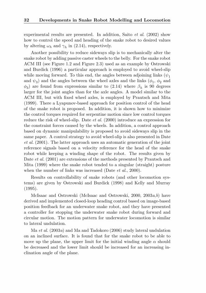
32 Developments in Snake Robot Modelling and Locomotion
experimental results are presented. In addition, Saito et al. (2002) showhow to control the speed and heading of the snake robot to desired valuesby altering !h and h in (2.14), respectively.
Another possibility to reduce sideways slip is to mechanically alter thesnake robot by adding passive caster wheels to the belly. For the snake robotACM III (see Figure 1.2 and Figure 2.3) used as an example by Ostrowskiand Burdick (1996) a particular approach is employed to avoid wheel-slipwhile moving forward. To this end, the angles between adjoining links ( 1and 3) and the angles between the wheel axles and the links (�1, �2 and�3) are found from expressions similar to (2.14) where �h is 90 degreeslarger for the joint angles than for the axle angles. A model similar to theACM III, but with �xed wheel axles, is employed by Prautsch and Mita(1999). There a Lyapunov-based approach for position control of the headof the snake robot is proposed. In addition, it is shown how to minimizethe control torques required for serpentine motion since low control torquesreduce the risk of wheel-slip. Date et al. (2000) introduce an expression forthe constraint forces caused by the wheels. In addition, a control approachbased on dynamic manipulability is proposed to avoid sideways slip in thesame paper. A control strategy to avoid wheel-slip is also presented in Dateet al. (2001). The latter approach uses an automatic generation of the jointreference signals based on a velocity reference for the head of the snakerobot while keeping a winding shape of the robot. The results given byDate et al. (2001) are extensions of the methods presented by Prautsch andMita (1999) where the snake robot tended to a singular (straight) posturewhen the number of links was increased (Date et al., 2000).
Results on controllability of snake robots (and other locomotion sys-tems) are given by Ostrowski and Burdick (1998) and Kelly and Murray(1995).
McIsaac and Ostrowski (McIsaac and Ostrowski, 2000, 2003a,b) havederived and implemented closed-loop heading control based on image-basedposition feedback for an underwater snake robot, and they have presenteda controller for stopping the underwater snake robot during forward andcircular motion. The motion pattern for underwater locomotion is similarto lateral undulation.
Ma et al. (2003a) and Ma and Tadokoro (2006) study lateral undulationon an inclined surface. It is found that for the snake robot to be able tomove up the plane, the upper limit for the initial winding angle � shouldbe decreased and the lower limit should be increased for an increasing in-clination angle of the plane.
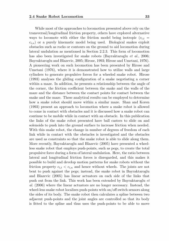
2.4 Snake Robot Locomotion 33
While most of the approaches to locomotion presented above rely on thetransversal/longitudinal friction property, others have explored alternativeways to locomote with either the friction model being isotropic (ci;t =ci;n) or a purely kinematic model being used. Biological snakes exploitobstacles such as rocks or contours on the ground to aid locomotion duringlateral undulation as mentioned in Section 2.2.3. This form of locomotionhas also been investigated for snake robots (Bayraktaroglu et al., 2006;Bayraktaroglu and Blazevic, 2005; Hirose, 1993; Hirose and Umetani, 1976).A pioneering work on such locomotion has been presented by Hirose andUmetani (1976), where it is demonstrated how to utilize walls and largecylinders to generate propulsive forces for a wheeled snake robot. Hirose(1993) analyses the gliding con�guration of a snake negotiating a cornerwithin a maze. In addition, he presents a relationship between the angle ofthe corner, the friction coe¢ cient between the snake and the walls of themaze and the distance between the contact points for contact between thesnake and the maze. These analytical results can be employed to determinehow a snake robot should move within a similar maze. Shan and Koren(1993) present an approach to locomotion where a snake robot is allowedto come in contact with obstacles and it is discussed how a snake robot cancontinue to be mobile while in contact with an obstacle. In this publicationthe links of the snake robot presented have ball casters to slide on andsolenoids to push into the ground surface to increase friction when needed.With this snake robot, the change in number of degrees of freedom of eachlink while in contact with the obstacles is investigated and the obstaclesare used as constraints so that the snake robot is able to slide along them.More recently, Bayraktaroglu and Blazevic (2005) have presented a wheel-less snake robot that employs push-points, such as pegs, to create the totalpropulsive force during a form of lateral undulation. Here, the ratio betweenlateral and longitudinal friction forces is disregarded, and this makes itpossible to build and develop motion patterns for snake robots without thefriction property ci;t < ci;n and hence without wheels. The joints are notbent to push against the pegs; instead, the snake robot in Bayraktarogluand Blazevic (2005) has linear actuators on each side of the links thatpush out from the link. This work has been extended by Bayraktaroglu etal. (2006) where the linear actuators are no longer necessary. Instead, thewheel-less snake robot localizes push-points with on/o¤switch sensors alongthe sides of its body. The snake robot then calculates a spline between twoadjacent push-points and the joint angles are controlled so that its bodyis �tted to the spline and thus uses the push-points to be able to move
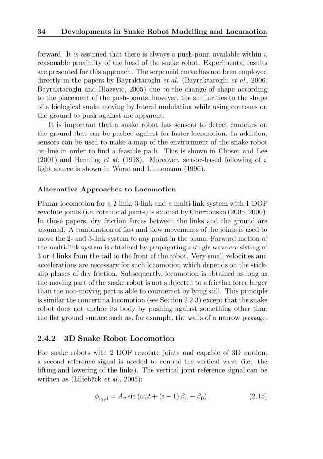
34 Developments in Snake Robot Modelling and Locomotion
forward. It is assumed that there is always a push-point available within areasonable proximity of the head of the snake robot. Experimental resultsare presented for this approach. The serpenoid curve has not been employeddirectly in the papers by Bayraktaroglu et al. (Bayraktaroglu et al., 2006;Bayraktaroglu and Blazevic, 2005) due to the change of shape accordingto the placement of the push-points, however, the similarities to the shapeof a biological snake moving by lateral undulation while using contours onthe ground to push against are apparent.
It is important that a snake robot has sensors to detect contours onthe ground that can be pushed against for faster locomotion. In addition,sensors can be used to make a map of the environment of the snake roboton-line in order to �nd a feasible path. This is shown in Choset and Lee(2001) and Henning et al. (1998). Moreover, sensor-based following of alight source is shown in Worst and Linnemann (1996).
Alternative Approaches to Locomotion
Planar locomotion for a 2-link, 3-link and a multi-link system with 1 DOFrevolute joints (i.e. rotational joints) is studied by Chernousko (2005, 2000).In those papers, dry friction forces between the links and the ground areassumed. A combination of fast and slow movements of the joints is used tomove the 2- and 3-link system to any point in the plane. Forward motion ofthe multi-link system is obtained by propagating a single wave consisting of3 or 4 links from the tail to the front of the robot. Very small velocities andaccelerations are necessary for such locomotion which depends on the stick-slip phases of dry friction. Subsequently, locomotion is obtained as long asthe moving part of the snake robot is not subjected to a friction force largerthan the non-moving part is able to counteract by lying still. This principleis similar the concertina locomotion (see Section 2.2.3) except that the snakerobot does not anchor its body by pushing against something other thanthe �at ground surface such as, for example, the walls of a narrow passage.
2.4.2 3D Snake Robot Locomotion
For snake robots with 2 DOF revolute joints and capable of 3D motion,a second reference signal is needed to control the vertical wave (i.e. thelifting and lowering of the links). The vertical joint reference signal can bewritten as (Liljebäck et al., 2005):
�vi;d = Av sin (!vt+ (i� 1)�v + �0) , (2.15)
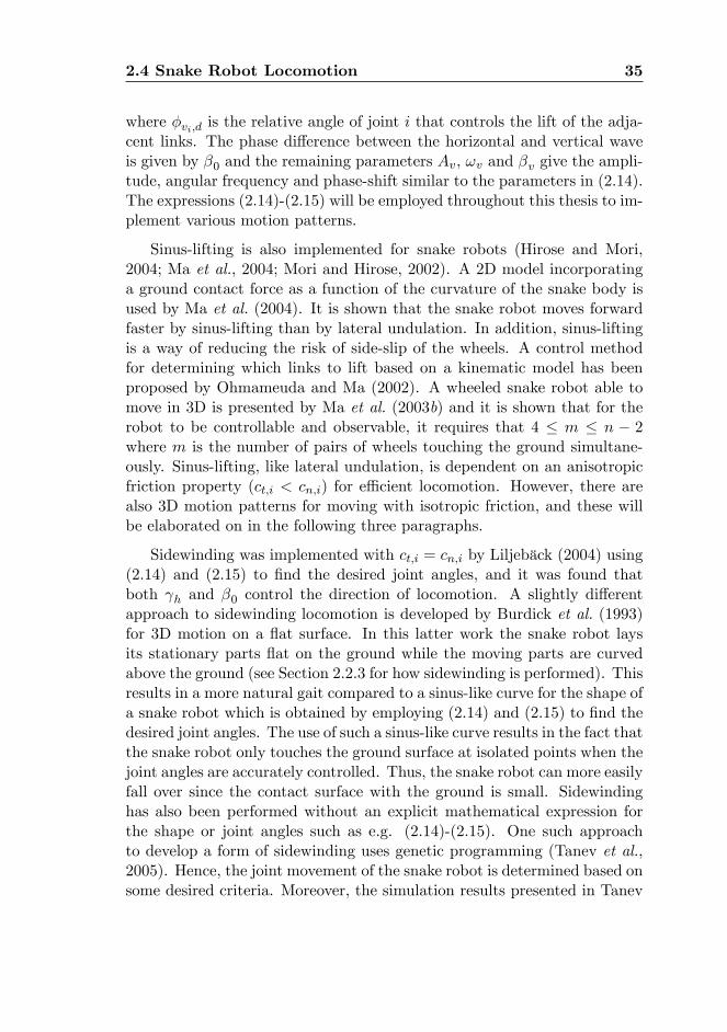
2.4 Snake Robot Locomotion 35
where �vi;d is the relative angle of joint i that controls the lift of the adja-cent links. The phase di¤erence between the horizontal and vertical waveis given by �0 and the remaining parameters Av, !v and �v give the ampli-tude, angular frequency and phase-shift similar to the parameters in (2.14).The expressions (2.14)-(2.15) will be employed throughout this thesis to im-plement various motion patterns.
Sinus-lifting is also implemented for snake robots (Hirose and Mori,2004; Ma et al., 2004; Mori and Hirose, 2002). A 2D model incorporatinga ground contact force as a function of the curvature of the snake body isused by Ma et al. (2004). It is shown that the snake robot moves forwardfaster by sinus-lifting than by lateral undulation. In addition, sinus-liftingis a way of reducing the risk of side-slip of the wheels. A control methodfor determining which links to lift based on a kinematic model has beenproposed by Ohmameuda and Ma (2002). A wheeled snake robot able tomove in 3D is presented by Ma et al. (2003b) and it is shown that for therobot to be controllable and observable, it requires that 4 � m � n � 2where m is the number of pairs of wheels touching the ground simultane-ously. Sinus-lifting, like lateral undulation, is dependent on an anisotropicfriction property (ct;i < cn;i) for e¢ cient locomotion. However, there arealso 3D motion patterns for moving with isotropic friction, and these willbe elaborated on in the following three paragraphs.
Sidewinding was implemented with ct;i = cn;i by Liljebäck (2004) using(2.14) and (2.15) to �nd the desired joint angles, and it was found thatboth h and �0 control the direction of locomotion. A slightly di¤erentapproach to sidewinding locomotion is developed by Burdick et al. (1993)for 3D motion on a �at surface. In this latter work the snake robot laysits stationary parts �at on the ground while the moving parts are curvedabove the ground (see Section 2.2.3 for how sidewinding is performed). Thisresults in a more natural gait compared to a sinus-like curve for the shape ofa snake robot which is obtained by employing (2.14) and (2.15) to �nd thedesired joint angles. The use of such a sinus-like curve results in the fact thatthe snake robot only touches the ground surface at isolated points when thejoint angles are accurately controlled. Thus, the snake robot can more easilyfall over since the contact surface with the ground is small. Sidewindinghas also been performed without an explicit mathematical expression forthe shape or joint angles such as e.g. (2.14)-(2.15). One such approachto develop a form of sidewinding uses genetic programming (Tanev et al.,2005). Hence, the joint movement of the snake robot is determined based onsome desired criteria. Moreover, the simulation results presented in Tanev
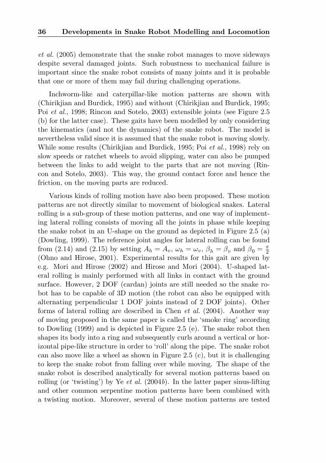
36 Developments in Snake Robot Modelling and Locomotion
et al. (2005) demonstrate that the snake robot manages to move sidewaysdespite several damaged joints. Such robustness to mechanical failure isimportant since the snake robot consists of many joints and it is probablethat one or more of them may fail during challenging operations.
Inchworm-like and caterpillar-like motion patterns are shown with(Chirikjian and Burdick, 1995) and without (Chirikjian and Burdick, 1995;Poi et al., 1998; Rincon and Sotelo, 2003) extensible joints (see Figure 2.5(b) for the latter case). These gaits have been modelled by only consideringthe kinematics (and not the dynamics) of the snake robot. The model isnevertheless valid since it is assumed that the snake robot is moving slowly.While some results (Chirikjian and Burdick, 1995; Poi et al., 1998) rely onslow speeds or ratchet wheels to avoid slipping, water can also be pumpedbetween the links to add weight to the parts that are not moving (Rin-con and Sotelo, 2003). This way, the ground contact force and hence thefriction, on the moving parts are reduced.
Various kinds of rolling motion have also been proposed. These motionpatterns are not directly similar to movement of biological snakes. Lateralrolling is a sub-group of these motion patterns, and one way of implement-ing lateral rolling consists of moving all the joints in phase while keepingthe snake robot in an U-shape on the ground as depicted in Figure 2.5 (a)(Dowling, 1999). The reference joint angles for lateral rolling can be foundfrom (2.14) and (2.15) by setting Ah = Av, !h = !v, �h = �v and �0 =
�2
(Ohno and Hirose, 2001). Experimental results for this gait are given bye.g. Mori and Hirose (2002) and Hirose and Mori (2004). U-shaped lat-eral rolling is mainly performed with all links in contact with the groundsurface. However, 2 DOF (cardan) joints are still needed so the snake ro-bot has to be capable of 3D motion (the robot can also be equipped withalternating perpendicular 1 DOF joints instead of 2 DOF joints). Otherforms of lateral rolling are described in Chen et al. (2004). Another wayof moving proposed in the same paper is called the �smoke ring�accordingto Dowling (1999) and is depicted in Figure 2.5 (e). The snake robot thenshapes its body into a ring and subsequently curls around a vertical or hor-izontal pipe-like structure in order to �roll�along the pipe. The snake robotcan also move like a wheel as shown in Figure 2.5 (c), but it is challengingto keep the snake robot from falling over while moving. The shape of thesnake robot is described analytically for several motion patterns based onrolling (or �twisting�) by Ye et al. (2004b). In the latter paper sinus-liftingand other common serpentine motion patterns have been combined witha twisting motion. Moreover, several of these motion patterns are tested
2.4 Snake Robot Locomotion 37
Figure 2.5: Various motion patterns implemented for snake robots: (a)U-shaped lateral rolling (moving towards the right), (b) travelling wave/caterpillar locomotion (moving the same way as the travelling wave, i.e.left or right), (c) the wheel (moving right or left), (d) bridge mode (movingright or left), and (e) �smoke ring�(moving up- or downward).
38 Developments in Snake Robot Modelling and Locomotion
by experiments and all tests show a mainly sideways motion of the snakerobot. Erkmen et al. (2002) have also elaborated on the twisting mode oflocomotion where an approach on how to make the snake robot walk usingits two ends as feet is described. This form of locomotion is called �bridgemode�and is illustrated in Figure 2.5 (d). In addition, a genetic algorithmis presented that handles how to move the snake robot from lying �at on theground to standing on its two ends without falling over. Descriptive �guresand explanations of the several gaits mentioned above, in addition to othermotion patterns, are given by Dowling (1999), Ohno and Hirose (2001) andMori and Hirose (2002). Moreover, movies of various snake robots duringlocomotion can be found on the web (Choset, 2007; Miller, 2007).
A snake robot, called the ACM-R5, with �ns with wheels on its link andthus capable of both swimming and land-based locomotion is presented byYamada et al. (2005). On the ground the snake robot moves by lateralrolling and lateral undulation. In the water it can move up and down,swim forward and turn. The details on the motion patterns are said to bereported at a later stage.
A snake robot needs to lift its body when, for example, climbing ormoving over high obstacles. However, the joint actuators can only producea limited torque. Hence, the snake robot links should be lifted in some�intelligent�manner to keep the necessary joint torques as low as possible.To this end, Nilsson (1997b, 1998) has developed an algorithm for liftingseveral links with limited joint torque. In addition, the snake robot mayutilize poles or other objects for climbing and a variant of the �smoke ring�in Figure 2.5 (e) has been proposed by Nilsson (1997a).
2.5 Discussion and Summary
Research on snake robots has increased the past ten to �fteen years, butthere are still many challenges to face both on modelling and control ofsnake robots in order to make them able to locomote intelligently throughunknown terrain. In this chapter we have seen a variety of approaches tomodelling and locomotion of snake robots and these will be summarized inthe following.
Since snake robots have a high number of degrees of freedom, carefulconsideration has to be taken to decide what model to use for a snake robotdepending on which aspect of snake robot locomotion is being studied.A planar and purely kinematic model is sometimes employed to describelateral undulation for a snake robot with passive caster wheels that do not
2.5 Discussion and Summary 39
slip. The use of a purely kinematic model simpli�es both the model and theanalysis of locomotion, and factors that contribute to locomotion are moreeasily highlighted. 3D models of the kinematics of snake robots withoutwheels are also developed and they are employed to study motion patternswhich also requires lifting and lowering (in addition to sideways motion) ofthe snake robot links. The kinematic description of snake robot locomotionwithout wheels is justi�ed by assuming low velocities and sometimes alsocertain friction properties (such as zero friction while gliding forward, butin�nite friction when pushed backward).
Although passive wheels help to justify the non-slip assumption (on thewheels) of some kinematic models, it can still be di¢ cult to control the jointtorques such that the wheels do not slip. Moreover, locomotion of snakerobots at high velocities require that the friction between the undersideof the snake robot and the ground surface is considered. Hence, there isa need for models that include the dynamics of snake robot locomotion.2D dynamical models are mainly used to describe lateral undulation withside-slip (i.e. without the idealized assumption of wheels that do not slip,or with no wheels at all). The friction force between the snake robot andthe ground surface is described as viscous-like friction or Coulomb friction,and Coulomb friction is usually modelled with sign-functions. However,such a sign-function does not allow for a non-zero friction force at zerovelocity (the stick-phase). Hence, a snake robot lying on an inclined planewill slide slowly downward. The directional friction property between thebelly of the snake robot can not always be realized due to varying groundconditions. To this end, simulation results of a planar snake robot movingby a promising scheme which consists of the snake robot pushing againstobstacles are presented, and the simulation results are obtained from thedynamic simulation software WorkingModel. However, the contact betweenthe snake robot and the obstacles are described with a compliant model, andit requires a sti¤ spring coe¢ cient to represent the contact between a (hard)obstacle and a (hard) snake robot link. This results in sti¤ di¤erentialequations which are cumbersome to solve numerically.
Mathematical models that include the dynamics of motion yield a moreaccurate description of the behaviour of the system. This is advantageouswith respect to simulation, but the models may get very large and un-manageable. Thus, the simplicity of an analytical analysis su¤ers. In 2Dmodels, certain properties of the system help to simplify the model, butnot all of these properties persist in 3D models. However, moving in, forexample, a shattered building is an inherently 3D experience and thus 3D
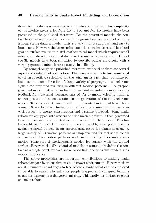
40 Developments in Snake Robot Modelling and Locomotion
dynamical models are necessary to simulate such motion. The complexityof the models grows a lot from 2D to 3D, and few 3D models have beenpresented in the published literature. For the presented models, the con-tact force between a snake robot and the ground surface is modelled usinga linear spring-damper model. This is a very intuitive approach and easy toimplement. However, the large spring coe¢ cient needed to resemble a hardground surface results in a sti¤ mathematical model which requires smallintegration steps to avoid instability in the numerical integration. One ofthe 3D models have been simpli�ed to describe planar movement with avarying ground contact force to study sinus-lifting.
By going through the published literature, we see that there are severalaspects of snake robot locomotion. The main concern is to �nd some kindof (often repetitive) reference for the joint angles such that the snake ro-bot moves in some direction. A large variety of preprogrammed referencesignals are proposed resulting in di¤erent motion patterns. The prepro-grammed motion patterns can be improved and extended by incorporatingfeedback from external measurements of, for example, velocity, heading,and/or position of the snake robot in the generation of the joint referenceangles. To some extent, such results are presented in the published liter-ature. Others focus on �nding optimal preprogrammed motion patternswith respect to energy consumption and distance travelled. Some snakerobots are equipped with sensors and the motion pattern is then generatedbased on continuously updated measurements from the sensors. This hasbeen achieved for a snake robot that moves forward by sensing and pushingagainst external objects in an experimental setup for planar motion. Alarge variety of 3D motion patterns are implemented for real snake robotsand some of these motion patterns are based on rolling. To simulate suchmotion, some sort of exoskeleton is needed for contact with the groundsurface. However, the 3D dynamical models presented only de�ne the con-tact as a single point for each snake robot link, and thus this renders suchmotion impossible.
The above approaches are important contributions to making snakerobots navigate by themselves in an unknown environment. However, thereare still numerous challenges to face before a snake robot can be employedto be able to search e¢ ciently for people trapped in a collapsed buildingor aid �re-�ghters on a dangerous mission. This motivates further researchon snake robots.
Chapter 3
Non-smooth Model of a 2DSnake Robot for Simulation
3.1 Introduction
The fastest biological snakes exploit roughness in the terrain for locomotion.They may push against rocks, branches, or other obstacles to move forwardmore e¢ ciently (Gray, 1946; Hirose, 1993). Snakes can also exploit the wallsof narrow passages for locomotion. Their mobility properties are interestingfor snake robot locomotion and give the motivation for investigating snakerobot obstacle aided locomotion. We de�ne obstacle aided locomotion assnake robot locomotion where snake robots utilize walls or other externalobjects, apart from the �at ground, for propulsion. In order to developsuch an obstacle aided locomotion scheme, we need a mathematical modelthat includes the interaction between the snake robot and a terrain withexternal objects for the snake robot to push against.
In this chapter we present a non-smooth (hybrid) modelling approachparticularly suitable for modelling snake robot motion in general and ob-stacle aided locomotion in particular. We use this approach to develop a 2Dmathematical model of a snake robot that can push against external objectsfor locomotion. The mathematical model is described in the framework ofnon-smooth dynamics and convex analysis (Brogliato, 1999; Glocker, 2001;Leine and Nijmeijer, 2004). The tools available in this framework that arenecessary for the mathematical modelling of a snake robot will be intro-duced and explained when necessary.
This chapter is based on Transeth et al. (2007b) and Transeth et al.(2008b) and it is organized as follows. Section 3.2 gives a short introduc-
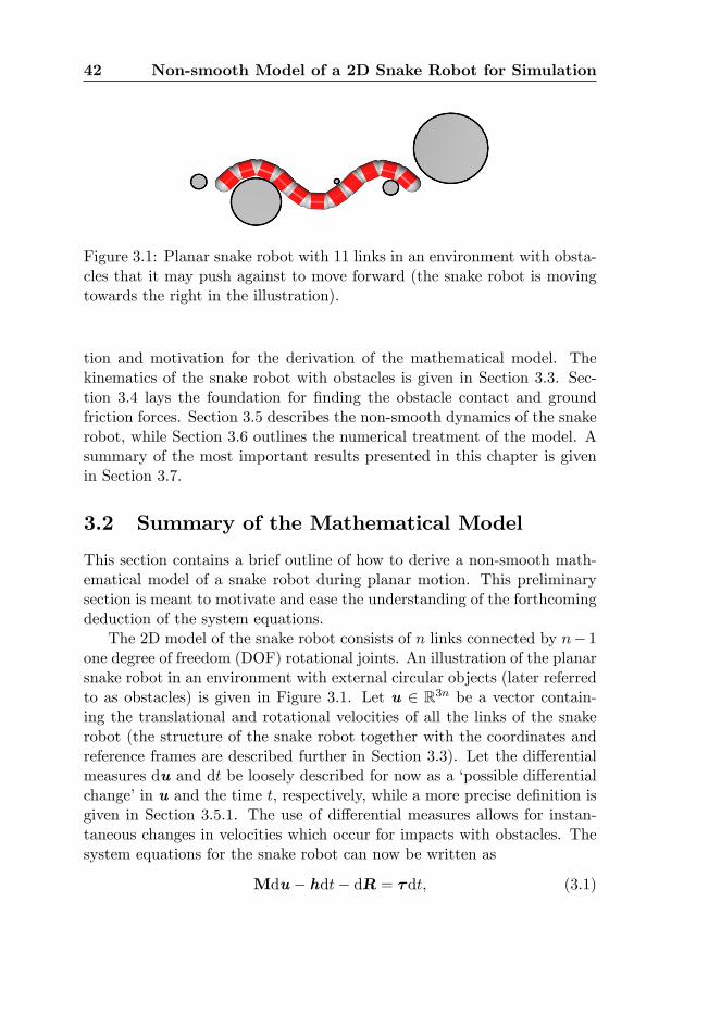
42 Non-smooth Model of a 2D Snake Robot for Simulation
Figure 3.1: Planar snake robot with 11 links in an environment with obsta-cles that it may push against to move forward (the snake robot is movingtowards the right in the illustration).
tion and motivation for the derivation of the mathematical model. Thekinematics of the snake robot with obstacles is given in Section 3.3. Sec-tion 3.4 lays the foundation for �nding the obstacle contact and groundfriction forces. Section 3.5 describes the non-smooth dynamics of the snakerobot, while Section 3.6 outlines the numerical treatment of the model. Asummary of the most important results presented in this chapter is givenin Section 3.7.
3.2 Summary of the Mathematical Model
This section contains a brief outline of how to derive a non-smooth math-ematical model of a snake robot during planar motion. This preliminarysection is meant to motivate and ease the understanding of the forthcomingdeduction of the system equations.
The 2D model of the snake robot consists of n links connected by n� 1one degree of freedom (DOF) rotational joints. An illustration of the planarsnake robot in an environment with external circular objects (later referredto as obstacles) is given in Figure 3.1. Let u 2 R3n be a vector contain-ing the translational and rotational velocities of all the links of the snakerobot (the structure of the snake robot together with the coordinates andreference frames are described further in Section 3.3). Let the di¤erentialmeasures du and dt be loosely described for now as a �possible di¤erentialchange�in u and the time t, respectively, while a more precise de�nition isgiven in Section 3.5.1. The use of di¤erential measures allows for instan-taneous changes in velocities which occur for impacts with obstacles. Thesystem equations for the snake robot can now be written as
Mdu� hdt� dR = �dt; (3.1)
3.2 Summary of the Mathematical Model 43
where (3.1) is termed the equality of measures (Moreau, 1988). Here M 2R3n�3n is the mass matrix, � 2 R3n contains all the joint actuator torques,h 2 R3n represents all the smooth forces (for example gravity, note thath = 03n�1 for the 2D model) and dR 2 R3n accounts for the normal contactforces/impulses from the obstacles, the Coulomb friction forces/impulsesand the bilateral constraint forces/impulses in the joints. Note: We allowin this chapter for instantaneous changes in velocities usually associatedwith collisions. Hence, the (normal contact/friction/constraint) �forces�are not always de�ned due to the in�nite accelerations. In these caseswe have impulses instead of forces. The non-smooth equality of measures(3.1) allows us to formulate in a uniform manner both the smooth andnon-smooth phases of motion. This is achieved partly by representing thecontact forces/impulses as contact impulse measures (these are included bydR in the equality of measures).
A substantial part of the beginning of this chapter is devoted to deduct-ing the force measure dR. Hence, let us brie�y look at how to derive thecontribution of the normal contact impulse measure between an obstaclej and the �rst link, in dR. Let dR1 2 R3 be the sum of contact impulsemeasures that directly a¤ect link 1 (i.e. the �rst three elements of dR).Then
dR1 = wH dPH +�friction and joint constraintimpulse measures
�; (3.2)
where dPH 2 R is the normal contact impulse measure from obstacle jon link 1 and wH 2 R3 is the corresponding generalized force direction(subscripts �j�and �1�are omitted for brevity).
Let gH 2 R be a function giving the shortest distance between link 1 andthe obstacle. Such a function is called a gap function (Glocker and Studer,2005). The gap function is the starting point for the systematic approach of�nding the impulse measures. The link and obstacle are separated if gH > 0,are in contact if gH = 0 and are penetrating each other if gH < 0. Hence,the relative velocity between link 1 and the obstacle along the shortest linebetween the two objects can be de�ned as H := _gH , and it is written, bycalculating _gH , on the form
H = wTHu1; (3.3)
where u1 is the velocity of link 1. Hence, by inspecting the expression for_gH and formulating it as (3.3) we �nd an expression for wH in (3.2). Thenormal contact impulse measure dPH is related to the relative velocity Hby employing a set-valued force law (see Section 3.5). The set-valuedness
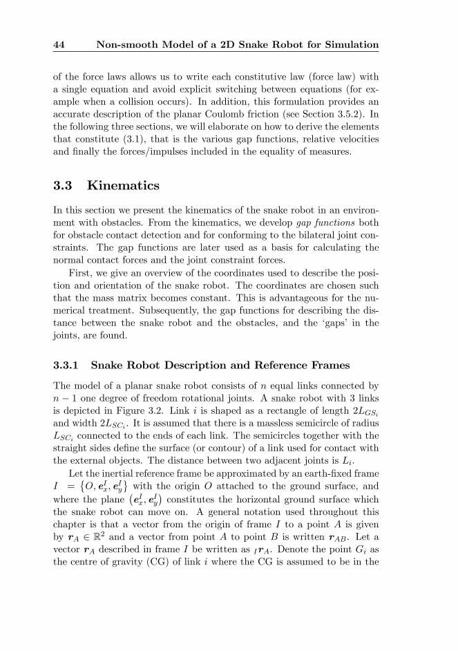
44 Non-smooth Model of a 2D Snake Robot for Simulation
of the force laws allows us to write each constitutive law (force law) witha single equation and avoid explicit switching between equations (for ex-ample when a collision occurs). In addition, this formulation provides anaccurate description of the planar Coulomb friction (see Section 3.5.2). Inthe following three sections, we will elaborate on how to derive the elementsthat constitute (3.1), that is the various gap functions, relative velocitiesand �nally the forces/impulses included in the equality of measures.
3.3 Kinematics
In this section we present the kinematics of the snake robot in an environ-ment with obstacles. From the kinematics, we develop gap functions bothfor obstacle contact detection and for conforming to the bilateral joint con-straints. The gap functions are later used as a basis for calculating thenormal contact forces and the joint constraint forces.
First, we give an overview of the coordinates used to describe the posi-tion and orientation of the snake robot. The coordinates are chosen suchthat the mass matrix becomes constant. This is advantageous for the nu-merical treatment. Subsequently, the gap functions for describing the dis-tance between the snake robot and the obstacles, and the �gaps� in thejoints, are found.
3.3.1 Snake Robot Description and Reference Frames
The model of a planar snake robot consists of n equal links connected byn � 1 one degree of freedom rotational joints. A snake robot with 3 linksis depicted in Figure 3.2. Link i is shaped as a rectangle of length 2LGSiand width 2LSCi . It is assumed that there is a massless semicircle of radiusLSCi connected to the ends of each link. The semicircles together with thestraight sides de�ne the surface (or contour) of a link used for contact withthe external objects. The distance between two adjacent joints is Li.
Let the inertial reference frame be approximated by an earth-�xed frameI =
�O;eIx; e
Iy
with the origin O attached to the ground surface, and
where the plane�eIx; e
Iy
�constitutes the horizontal ground surface which
the snake robot can move on. A general notation used throughout thischapter is that a vector from the origin of frame I to a point A is givenby rA 2 R2 and a vector from point A to point B is written rAB. Let avector rA described in frame I be written as IrA. Denote the point Gi asthe centre of gravity (CG) of link i where the CG is assumed to be in the
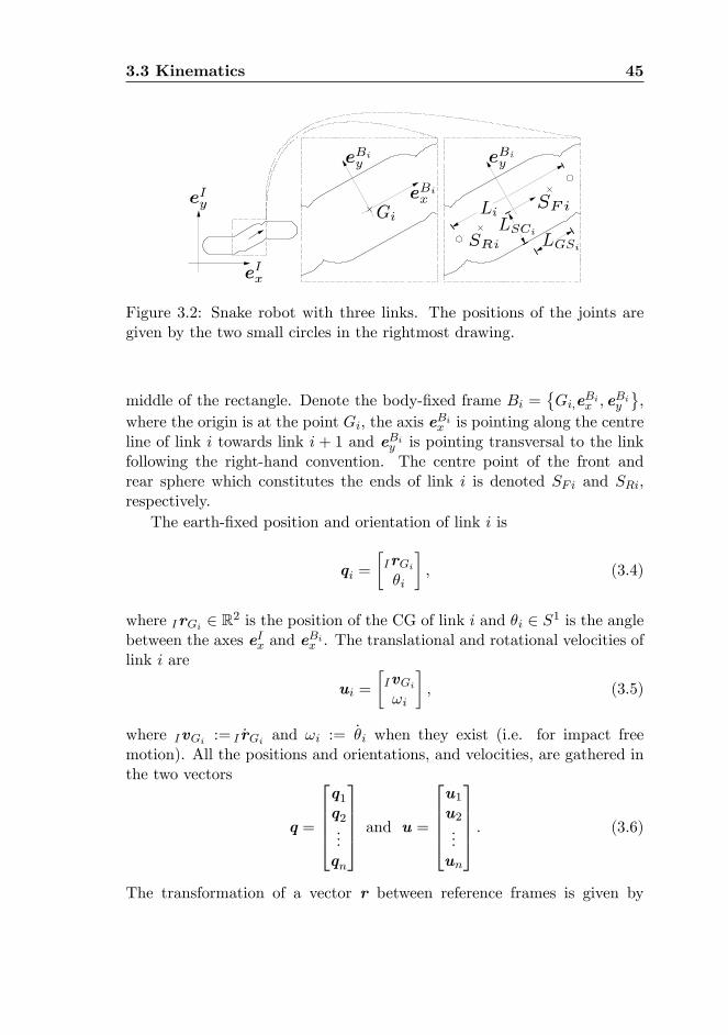
3.3 Kinematics 45
Figure 3.2: Snake robot with three links. The positions of the joints aregiven by the two small circles in the rightmost drawing.
middle of the rectangle. Denote the body-�xed frame Bi =�Gi;e
Bix ; e
Biy
,
where the origin is at the point Gi, the axis eBix is pointing along the centreline of link i towards link i + 1 and eBiy is pointing transversal to the linkfollowing the right-hand convention. The centre point of the front andrear sphere which constitutes the ends of link i is denoted SFi and SRi,respectively.
The earth-�xed position and orientation of link i is
qi =
�IrGi�i
�; (3.4)
where IrGi 2 R2 is the position of the CG of link i and �i 2 S1 is the anglebetween the axes eIx and e
Bix . The translational and rotational velocities of
link i are
ui =
�IvGi!i
�; (3.5)
where IvGi := I _rGi and !i := _�i when they exist (i.e. for impact freemotion). All the positions and orientations, and velocities, are gathered inthe two vectors
q =
26664q1q2...qn
37775 and u =
26664u1u2...un
37775 : (3.6)
The transformation of a vector r between reference frames is given by
46 Non-smooth Model of a 2D Snake Robot for Simulation
Figure 3.3: Snake robot with three links depicted with obstacle j = 1 closestto link i = 3.
Ir = RIBi Bir where the rotation matrix is
RIBi =
�cos �i � sin �isin �i cos �i
�. (3.7)
External �xed objects are included in the model for the snake robot topush against. Each obstacle j, j = 1; 2; : : : ; �, is shaped as a circle in theplane with radius LHj and midpoint Hj , see Figure 3.3. The gap functiongHij in the �gure is described in the following.
3.3.2 Gap Functions for Obstacle Contact
We begin this section by giving an example of what a gap function is usedfor, then we introduce the gap functions for contact between the snakerobot and the obstacles.
Example 3.1 (Gap Function) Consider two convex rigid bodies 1 and 2.Now, we want to determine whether Body 1 is in contact with Body 2. Thiscan be achieved by determining whether the minimal distance between thetwo bodies is equal to zero. The function that gives us the minimal distanceis called a gap function (Glocker and Studer, 2005) and the point on Body1 that is closest to Body 2 is called a (possible) contact point. Apart fromdetermining if two rigid bodies are in contact, the gap function will also beused as a basis for calculating the direction and size of the forces involvedin the contact.
3.3 Kinematics 47
The gap function gHij gives the shortest distance between link i andobstacle j as illustrated in Figure 3.3 and is used to detect whether the twobodies are in contact. In addition, this gap function will be used later as abasis for calculating the forces involved in the contact.
Link i can, at any time-instance, only touch a convex obstacle j at asingle point, resulting in a contact point that may move across the entiresurface of a link. The surface (or contour) of a link consists of three parts:the rectangle, the front semicircle and the rear semicircle. Hence, we seethat we need to �nd two separate kinds of gap functions for each linkdepending on which part of the link is closest to the obstacle. In particular,we need to �nd the shortest distance between a rectangle and a circle, andbetween two circles. This approach provides us with a moving contactpoint. Hence, the obstacle can come in contact with the snake robot at anypoint and the e¤ect the contact force has on a snake robot link is thereforemodelled accurately.
Distance Between Rectangle Part and Obstacle
When the rectangle-shaped part of link i is closest to obstacle j, we needto investigate the distance between a line (the eBix -axis) and the centre ofthe obstacle Hj . The shortest distance between the eBix -axis and Hj is
dij = (IrGi � IrHj)TIeBiy . (3.8)
Hence, the gap function when the rectangle part of link i is closest toobstacle j is
gHij = jdij j ��LHj + LSCi
�. (3.9)
Distance Between Circle Part and Obstacle
The minimal distance between the circle part of link i and obstacle j isfound from the gap function
gHij = IrHjSi
� �LHj + LSCi� (3.10)
where
rHjSi = rGi + rGiSFi � rHj or (3.11)
rHjSi = rGi + rGiSRi � rHj (3.12)
depending on whether the front or rear part of the link is closest to theobstacle, respectively. In addition, rGiSFi = LGSie
Bix , rGiSRi = �LGSieBix
and we de�ne k�k := k�k2.
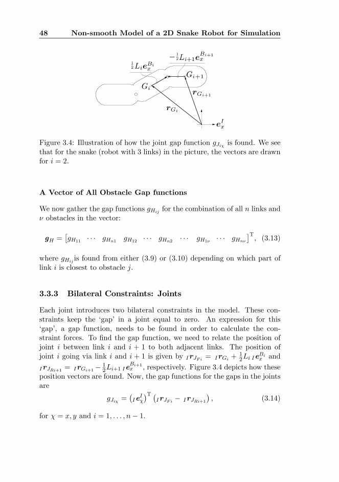
48 Non-smooth Model of a 2D Snake Robot for Simulation
Figure 3.4: Illustration of how the joint gap function gJi� is found. We seethat for the snake (robot with 3 links) in the picture, the vectors are drawnfor i = 2.
A Vector of All Obstacle Gap functions
We now gather the gap functions gHij for the combination of all n links and� obstacles in the vector:
gH =�gH11 � � � gHn1 gH12 � � � gHn2 � � � gH1� � � � gHn�
�T; (3.13)
where gHij is found from either (3.9) or (3.10) depending on which part oflink i is closest to obstacle j.
3.3.3 Bilateral Constraints: Joints
Each joint introduces two bilateral constraints in the model. These con-straints keep the �gap� in a joint equal to zero. An expression for this�gap�, a gap function, needs to be found in order to calculate the con-straint forces. To �nd the gap function, we need to relate the position ofjoint i between link i and i + 1 to both adjacent links. The position ofjoint i going via link i and i + 1 is given by IrJFi = IrGi +
12Li Ie
Bix and
IrJRi+1 = IrGi+1� 12Li+1 Ie
Bi+1x , respectively. Figure 3.4 depicts how these
position vectors are found. Now, the gap functions for the gaps in the jointsare
gJi� =�IeI�
�T �IrJFi � IrJRi+1
�; (3.14)
for � = x; y and i = 1; : : : ; n� 1.
3.4 Contact Constraints on Velocity Level 49
3.4 Contact Constraints on Velocity Level
In this section the relative velocities between the snake robot, and theobstacles and the ground, are found by taking the time-derivative (whenthey exist) of the corresponding gap functions. The relative velocities areemployed to calculate the normal contact forces involved in the contactbetween the snake robot and the obstacles (Le Saux et al., 2005; Leineand Nijmeijer, 2004). Also, the relative velocities are employed to �nd thefriction forces between the ground and the snake robot, and the bilateralconstraint forces in the joints. This is shown in Section 3.5.2.
3.4.1 Relative Velocity Between an Obstacle and a Link
The relative velocity between a link i and an obstacle j is de�ned as Hij := _gHij (when the time-derivative exists). As for the gap functions,the expression for the relative velocity depends on which part of the link isclosest to the obstacle.
Rectangle Part Closest to Obstacle
If the rectangle-shaped part of link i is closest to obstacle j, then therelative velocity between these two convex objects Hij := _gHij is found, byemploying (3.9), as
Hij =ddtjdij j =) Hij = w
THijui; (3.15)
where dij is given in (3.8) and the generalized force direction is
wTHij = sign (dij)
��IeBiy
�T �IrHj � IrGi
�T �cos (�i)sin (�i)
��ui; (3.16)
for i = 1; : : : ; n and j = 1; : : : ; �.
Circle Part Closest to Obstacle
The gap function (3.10) is employed to de�ne the relative velocity Hij :=_gHij when one of the circle-shaped parts of link i is closest to obstacle j.By de�nition, the relative velocity is
Hij =ddt
IrHjSi
=) Hij = wTHijui; (3.17)
50 Non-smooth Model of a 2D Snake Robot for Simulation
where the generalized force direction is, for i = 1; : : : ; n and j = 1; : : : ; �,
wTHij =IrHjSi IrHjSi
�I2�2 RIBiDBirGiSi
�; (3.18)
D =
�0 �11 0
�; I2�2 =
�1 00 1
�; (3.19)
and IrHjSi is given by (3.11) or (3.12) and rGiSi is equal to either BirGiSFior BirGiSRi depending on whether the front (Fi) or rear (Ri) part of thelink is closest to the obstacle as described in Section 3.3.2. To �nd theexpression for wTHij in (3.18) we have employed the following identities:
ddt
IrHjSi
=IrHjSi IrHjSi
ddt IrHjSi ; (3.20)
ddtRIBi = RI
BiD: (3.21)
Notice that we have employed the same notation for wHij in (3.16) and(3.18) to reduce the number of subscripts.
Vector of All Relative Velocities for Obstacles
We gather the relative velocities Hij for all n links and � obstacles in thevector
H =WTHu 2 Rn� ; (3.22)
where
H =� H11 � � � Hn1 H12 � � � Hn2 � � � H1� � � � Hn�
�T; (3.23)
WH =�WH1 � � � WH�
�2 R3n�n� ; (3.24)
and
WHj =
266664wH1j 03�1 � � � 03�1
03�1 wH2j. . .
......
. . . . . . 03�103�1 � � � 03�1 wHnj
377775 2 R3n�n. (3.25)
Depending on which part of the link is closest to the obstacle, wHij isobtained either from (3.16) or (3.18).
3.4 Contact Constraints on Velocity Level 51
3.4.2 Tangential Relative Velocity
The tangential relative velocities between a link i and the ground is pre-sented here. For the case of the planar snake robot, these velocities arethe velocities of the centre of gravity Gi for each link with respect to theearth-�xed coordinate axis
�eIx; e
Iy
�. The relative velocities will later be
employed to �nd the friction forces between the link and the ground. Westart by �nding the tangential relative velocities parallel to the eIx and e
Iy-
axis. These are denoted for link i by 0Tix and 0Tiy, respectively. However,
in order to easily �nd the friction forces longitudinal and lateral to eachlink, we need to derive the tangential relative velocities longitudinal Tixand lateral Tiy to each link.
The tangential relative velocities parallel to the eIx and eIy-axis are
0Ti� =�IeI�
�TIvGi =) 0Ti� =
�w0Ti�
�Tui; (3.26)
where the generalized force direction is�w0Ti�
�T=h�IeI�
�T0i; (3.27)
for � = x; y and i = 1; : : : ; n. The two relative velocities are combined inone vector so that
0Ti =�W0
Ti
�Tui; (3.28)
where
0Ti =
� 0Tix 0Tiy
�2 R2; W0
Ti =hw0Tix w0Tiy
i2 R3�2: (3.29)
The tangential relative velocities along the eBix and eBiy -axis can nowbe found as follows. De�ne
Ti =
� Tix Tiy
�: (3.30)
Then, by employing the rotation matrix RIBi
in (3.7), we have that 0Ti = RI
Bi Ti . Hence,
Ti =WTTiui; (3.31)
whereWTi =W
0TiR
IBi ; (3.32)
for i = 1; : : : ; n.
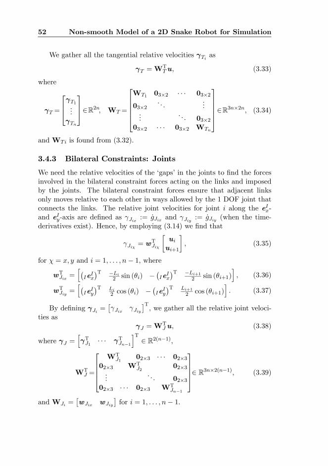
52 Non-smooth Model of a 2D Snake Robot for Simulation
We gather all the tangential relative velocities Ti as
T =WTTu; (3.33)
where
T =
264 T1... Tn
3752R2n; WT =
266664WT1 03�2 � � � 03�2
03�2. . .
......
. . . 03�203�2 � � � 03�2 WTn
3777752R3n�2n; (3.34)
andWTi is found from (3.32).
3.4.3 Bilateral Constraints: Joints
We need the relative velocities of the �gaps�in the joints to �nd the forcesinvolved in the bilateral constraint forces acting on the links and imposedby the joints. The bilateral constraint forces ensure that adjacent linksonly moves relative to each other in ways allowed by the 1 DOF joint thatconnects the links. The relative joint velocities for joint i along the eIx-and eIy-axis are de�ned as Jix := _gJix and Jiy := _gJiy (when the time-derivatives exist). Hence, by employing (3.14) we �nd that
Ji� = wTJi�
�uiui+1
�; (3.35)
for � = x; y and i = 1; : : : ; n� 1, where
wTJix =h�IeIx
�T �Li2 sin (�i) �
�IeIx
�T �Li+12 sin (�i+1)
i; (3.36)
wTJiy =h�IeIy
�T Li2 cos (�i) �
�IeIy
�T Li+12 cos (�i+1)
i. (3.37)
By de�ning Ji =� Jix Jiy
�T, we gather all the relative joint veloci-
ties as J =W
TJu; (3.38)
where J =h TJ1 � � � TJn�1
iT2 R2(n�1),
WTJ =
26664WT
J102�3 � � � 02�3
02�3 WTJ2
02�3...
. . . 02�302�3 � � � 02�3 WT
Jn�1
377752 R3n�2(n�1); (3.39)
andWJi =�wJix wJiy
�for i = 1; : : : ; n� 1.
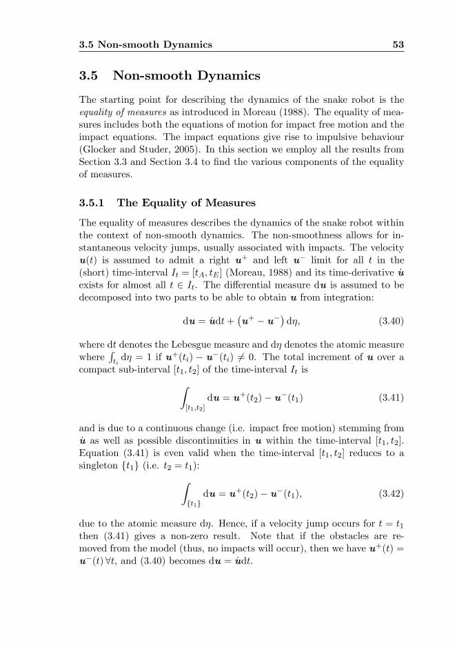
3.5 Non-smooth Dynamics 53
3.5 Non-smooth Dynamics
The starting point for describing the dynamics of the snake robot is theequality of measures as introduced in Moreau (1988). The equality of mea-sures includes both the equations of motion for impact free motion and theimpact equations. The impact equations give rise to impulsive behaviour(Glocker and Studer, 2005). In this section we employ all the results fromSection 3.3 and Section 3.4 to �nd the various components of the equalityof measures.
3.5.1 The Equality of Measures
The equality of measures describes the dynamics of the snake robot withinthe context of non-smooth dynamics. The non-smoothness allows for in-stantaneous velocity jumps, usually associated with impacts. The velocityu(t) is assumed to admit a right u+ and left u� limit for all t in the(short) time-interval It = [tA; tE ] (Moreau, 1988) and its time-derivative _uexists for almost all t 2 It. The di¤erential measure du is assumed to bedecomposed into two parts to be able to obtain u from integration:
du = _udt+�u+ � u�
�d�; (3.40)
where dt denotes the Lebesgue measure and d� denotes the atomic measurewhere
Rtid� = 1 if u+(ti) � u�(ti) 6= 0. The total increment of u over a
compact sub-interval [t1; t2] of the time-interval It isZ[t1;t2]
du = u+(t2)� u�(t1) (3.41)
and is due to a continuous change (i.e. impact free motion) stemming from_u as well as possible discontinuities in u within the time-interval [t1; t2].Equation (3.41) is even valid when the time-interval [t1; t2] reduces to asingleton ft1g (i.e. t2 = t1):Z
ft1gdu = u+(t2)� u�(t1); (3.42)
due to the atomic measure d�. Hence, if a velocity jump occurs for t = t1then (3.41) gives a non-zero result. Note that if the obstacles are re-moved from the model (thus, no impacts will occur), then we have u+(t) =u�(t)8t, and (3.40) becomes du = _udt.
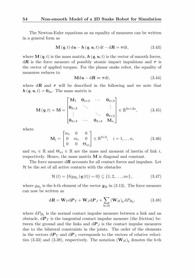
54 Non-smooth Model of a 2D Snake Robot for Simulation
The Newton-Euler equations as an equality of measures can be writtenin a general form as
M (q; t) du� h (q;u; t) dt� dR = �dt; (3.43)
whereM (q; t) is the mass matrix, h (q;u; t) is the vector of smooth forces,dR is the force measure of possibly atomic impact impulsions and � isthe vector of applied torques. For the planar snake robot, the equality ofmeasures reduces to
Mdu� dR = �dt; (3.44)
where dR and � will be described in the following and we note thath (q;u; t) = 03n. The mass matrix is
M (q; t) =M =
266664M1 03�3 � � � 03�3
03�3. . .
......
. . . 03�303�3 � � � 03�3 Mn
377775 2 R3n�3n; (3.45)
where
Mi =
24mi 0 00 mi 00 0 � i
35 2 R3�3; i = 1; : : : n; (3.46)
and mi 2 R and � i 2 R are the mass and moment of inertia of link i,respectively. Hence, the mass matrix M is diagonal and constant.
The force measure dR accounts for all contact forces and impulses. LetH be the set of all active contacts with the obstacles
H (t) = fbjgHb (q (t)) = 0g � f1; 2; : : : ; n�g ; (3.47)
where gHb is the b-th element of the vector gH in (3.13). The force measurecan now be written as
dR =WTdP T +WJdP J +Xb2H
(WH)b dPHb ; (3.48)
where dPHb is the normal contact impulse measure between a link and anobstacle, dP T is the tangential contact impulse measure (the friction) be-tween the ground and the links and dP J is the contact impulse measuresdue to the bilateral constraints in the joints. The order of the elementsin the vectors dP T and dP J corresponds to the vectors of relative veloci-ties (3.33) and (3.38), respectively. The notation (WH)b denotes the b-th
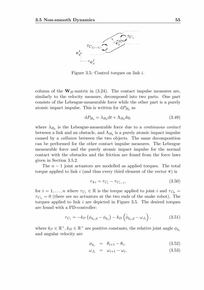
3.5 Non-smooth Dynamics 55
Figure 3.5: Control torques on link i.
column of the WH -matrix in (3.24). The contact impulse measures are,similarly to the velocity measure, decomposed into two parts. One partconsists of the Lebesgue-measurable force while the other part is a purelyatomic impact impulse. This is written for dPHb as
dPHb = �Hbdt+ �Hbd�; (3.49)
where �Hb is the Lebesgue-measurable force due to a continuous contactbetween a link and an obstacle, and �Hb is a purely atomic impact impulsecaused by a collision between the two objects. The same decompositioncan be performed for the other contact impulse measures. The Lebesguemeasurable force and the purely atomic impact impulse for the normalcontact with the obstacles and the friction are found from the force lawsgiven in Section 3.5.2.
The n � 1 joint actuators are modelled as applied torques. The totaltorque applied to link i (and thus every third element of the vector � ) is
�3�i = �Ci � �Ci�1 ; (3.50)
for i = 1; : : : ; n where �Ci 2 R is the torque applied to joint i and �C0 =�Cn = 0 (there are no actuators at the two ends of the snake robot). Thetorques applied to link i are depicted in Figure 3.5. The desired torquesare found with a PD-controller:
�Ci = �kP��hi;d � �hi
�� kD
�_�hi;d � !Ji
�; (3.51)
where kP 2 R+; kD 2 R+ are positive constants, the relative joint angle �hiand angular velocity are
�hi = �i+1 � �i; (3.52)
!Ji = !i+1 � !i; (3.53)
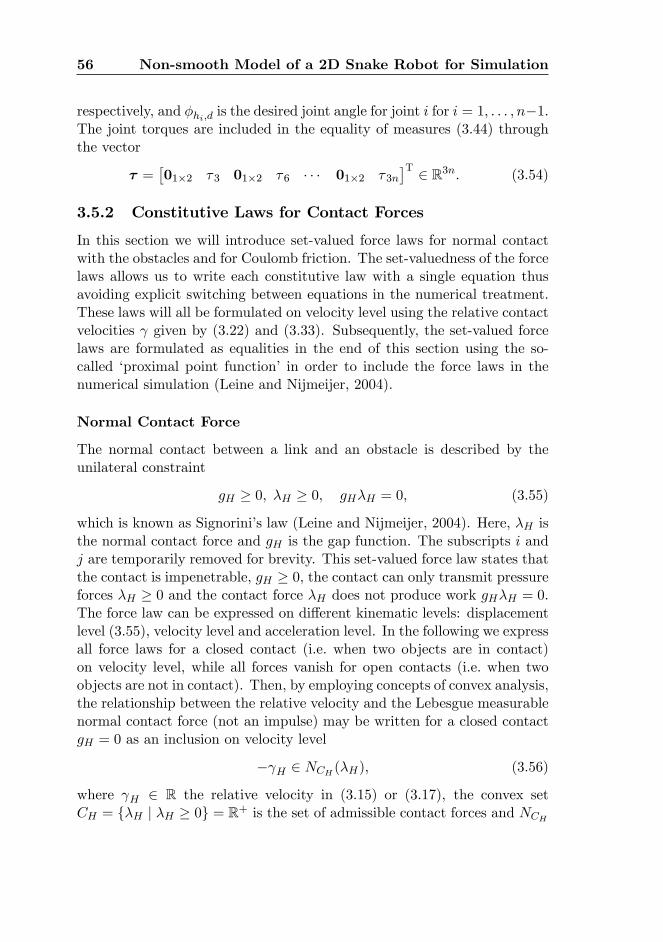
56 Non-smooth Model of a 2D Snake Robot for Simulation
respectively, and �hi;d is the desired joint angle for joint i for i = 1; : : : ; n�1.The joint torques are included in the equality of measures (3.44) throughthe vector
� =�01�2 �3 01�2 �6 � � � 01�2 �3n
�T 2 R3n: (3.54)
3.5.2 Constitutive Laws for Contact Forces
In this section we will introduce set-valued force laws for normal contactwith the obstacles and for Coulomb friction. The set-valuedness of the forcelaws allows us to write each constitutive law with a single equation thusavoiding explicit switching between equations in the numerical treatment.These laws will all be formulated on velocity level using the relative contactvelocities given by (3.22) and (3.33). Subsequently, the set-valued forcelaws are formulated as equalities in the end of this section using the so-called �proximal point function� in order to include the force laws in thenumerical simulation (Leine and Nijmeijer, 2004).
Normal Contact Force
The normal contact between a link and an obstacle is described by theunilateral constraint
gH � 0; �H � 0; gH�H = 0; (3.55)
which is known as Signorini�s law (Leine and Nijmeijer, 2004). Here, �H isthe normal contact force and gH is the gap function. The subscripts i andj are temporarily removed for brevity. This set-valued force law states thatthe contact is impenetrable, gH � 0, the contact can only transmit pressureforces �H � 0 and the contact force �H does not produce work gH�H = 0.The force law can be expressed on di¤erent kinematic levels: displacementlevel (3.55), velocity level and acceleration level. In the following we expressall force laws for a closed contact (i.e. when two objects are in contact)on velocity level, while all forces vanish for open contacts (i.e. when twoobjects are not in contact). Then, by employing concepts of convex analysis,the relationship between the relative velocity and the Lebesgue measurablenormal contact force (not an impulse) may be written for a closed contactgH = 0 as an inclusion on velocity level
� H 2 NCH (�H); (3.56)
where H 2 R the relative velocity in (3.15) or (3.17), the convex setCH = f�H j �H � 0g = R+ is the set of admissible contact forces and NCH
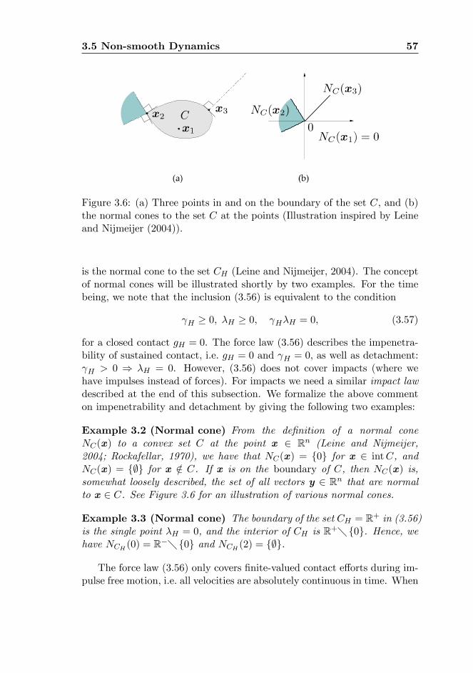
3.5 Non-smooth Dynamics 57
Figure 3.6: (a) Three points in and on the boundary of the set C, and (b)the normal cones to the set C at the points (Illustration inspired by Leineand Nijmeijer (2004)).
is the normal cone to the set CH (Leine and Nijmeijer, 2004). The conceptof normal cones will be illustrated shortly by two examples. For the timebeing, we note that the inclusion (3.56) is equivalent to the condition
H � 0; �H � 0; H�H = 0; (3.57)
for a closed contact gH = 0. The force law (3.56) describes the impenetra-bility of sustained contact, i.e. gH = 0 and H = 0, as well as detachment: H > 0 ) �H = 0. However, (3.56) does not cover impacts (where wehave impulses instead of forces). For impacts we need a similar impact lawdescribed at the end of this subsection. We formalize the above commenton impenetrability and detachment by giving the following two examples:
Example 3.2 (Normal cone) From the de�nition of a normal coneNC(x) to a convex set C at the point x 2 Rn (Leine and Nijmeijer,2004; Rockafellar, 1970), we have that NC(x) = f0g for x 2 intC, andNC(x) = f;g for x =2 C. If x is on the boundary of C, then NC(x) is,somewhat loosely described, the set of all vectors y 2 Rn that are normalto x 2 C. See Figure 3.6 for an illustration of various normal cones.
Example 3.3 (Normal cone) The boundary of the set CH = R+ in (3.56)is the single point �H = 0, and the interior of CH is R+� f0g. Hence, wehave NCH (0) = R�� f0g and NCH (2) = f;g.
The force law (3.56) only covers �nite-valued contact e¤orts during im-pulse free motion, i.e. all velocities are absolutely continuous in time. When
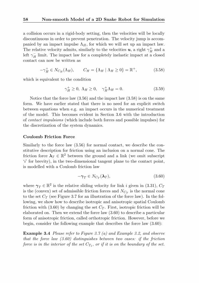
58 Non-smooth Model of a 2D Snake Robot for Simulation
a collision occurs in a rigid-body setting, then the velocities will be locallydiscontinuous in order to prevent penetration. The velocity jump is accom-panied by an impact impulse �H , for which we will set up an impact law.The relative velocity admits, similarly to the velocities u, a right +H and aleft �H limit. The impact law for a completely inelastic impact at a closedcontact can now be written as
� +H 2 NCH (�H); CH = f�H j �H � 0g = R+; (3.58)
which is equivalent to the condition
+H � 0; �H � 0; +H�H = 0: (3.59)
Notice that the force law (3.56) and the impact law (3.58) is on the sameform. We have earlier stated that there is no need for an explicit switchbetween equations when e.g. an impact occurs in the numerical treatmentof the model. This becomes evident in Section 3.6 with the introductionof contact impulsions (which include both forces and possible impulses) forthe discretization of the system dynamics.
Coulomb Friction Force
Similarly to the force law (3.56) for normal contact, we describe the con-stitutive description for friction using an inclusion on a normal cone. Thefriction force �T 2 R2 between the ground and a link (we omit subscript�i�for brevity), in the two-dimensional tangent plane to the contact point,is modelled with a Coulomb friction law
� T 2 NCT (�T ); (3.60)
where T 2 R2 is the relative sliding velocity for link i given in (3.31), CTis the (convex) set of admissible friction forces and NCT is the normal coneto the set CT (see Figure 3.7 for an illustration of the force law). In the fol-lowing, we show how to describe isotropic and anisotropic spatial Coulombfriction with (3.60) by changing the set CT . First, isotropic friction will beelaborated on. Then we extend the force law (3.60) to describe a particularform of anisotropic friction, called orthotropic friction. However, before webegin, consider the following example that describes the force law (3.60):
Example 3.4 Please refer to Figure 3.7 (a) and Example 3.2, and observethat the force law (3.60) distinguishes between two cases: if the frictionforce is in the interior of the set CT1, or if it is on the boundary of the set.
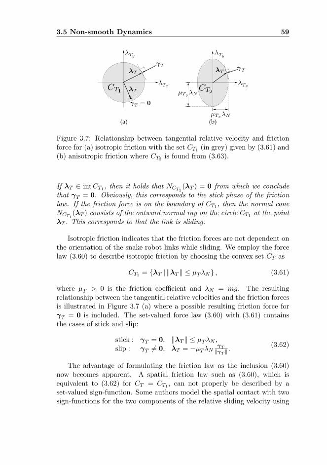
3.5 Non-smooth Dynamics 59
Figure 3.7: Relationship between tangential relative velocity and frictionforce for (a) isotropic friction with the set CT1 (in grey) given by (3.61) and(b) anisotropic friction where CT2 is found from (3.63).
If �T 2 intCT1, then it holds that NCT1(�T ) = 0 from which we conclude
that T = 0. Obviously, this corresponds to the stick phase of the frictionlaw. If the friction force is on the boundary of CT1, then the normal coneNCT1
(�T ) consists of the outward normal ray on the circle CT1 at the point�T . This corresponds to that the link is sliding.
Isotropic friction indicates that the friction forces are not dependent onthe orientation of the snake robot links while sliding. We employ the forcelaw (3.60) to describe isotropic friction by choosing the convex set CT as
CT1 = f�T j k�T k � �T�Ng ; (3.61)
where �T > 0 is the friction coe¢ cient and �N = mg. The resultingrelationship between the tangential relative velocities and the friction forcesis illustrated in Figure 3.7 (a) where a possible resulting friction force for T = 0 is included. The set-valued force law (3.60) with (3.61) containsthe cases of stick and slip:
stick : T = 0; k�T k � �T�N ;slip : T 6= 0; �T = ��T�N
Tk T k
:(3.62)
The advantage of formulating the friction law as the inclusion (3.60)now becomes apparent. A spatial friction law such as (3.60), which isequivalent to (3.62) for CT = CT1 , can not properly be described by aset-valued sign-function. Some authors model the spatial contact with twosign-functions for the two components of the relative sliding velocity using
60 Non-smooth Model of a 2D Snake Robot for Simulation
two friction coe¢ cients �Tx and �Ty (Ma et al., 2003a; Saito et al., 2002).This results however directly in an anisotropic friction law, as the fric-tion force and the sliding velocity do no longer point in opposite directions(even for �Tx = �Ty). Then such a double-sign-function force law corre-sponds to (3.60) with CT being a rectangle with length 2�Tx�N and width2�Ty�N . Also, the (set-valued) sign function can be approximated with asmooth function, for example some arctangent function. This results in avery steep slope of the friction curve near zero relative velocity. Such anapproach is very cumbersome for two reasons. First of all, stiction can notproperly be described: an object on a slope will with a smoothened frictionlaw always slide. Secondly, the very steep slope of the friction curve causesthe di¤erential equations of motion to become numerically sti¤. Summaris-ing, we see that (3.60) or (3.62) describes spatial Coulomb friction takingisotropy and stiction properly into account. We prefer using (3.60) insteadof (3.62), because the latter becomes not well conditioned for very small T when used in numerics. Note also that the force laws for Coulombfriction (3.60) and normal contact with the obstacles (3.56) have the samemathematical form. Moreover, the inclusion (3.60) is much more generalsince we can easily change the convex set CT to get a di¤erent (and henceanisotropic) friction model.
Orthotropic friction (which is a particular form of anisotropic friction)can be described by the force law (3.60) with the set CT being the equal tothe set
CT2 =
8><>:�T j �2Tx��Tx�N
�2 + �2Ty��Ty�N
�2 � 19>=>; ; (3.63)
where �T =��Tx �Ty
�T, and �Tx ; �Ty > 0 are directional friction coe¢ -
cients along the eBix - and eBiy -axis, respectively. The relationship between
the direction of the tangential relative velocity and the direction of the cor-responding friction force is illustrated in Figure 3.7 (b) for �Tx < �Ty . Notethat for �Tx = �Ty = �T , the set CT2 is equal to CT1 .
While the force law (3.60) only describes the Coulomb friction duringimpulse free motion, we also need a force law for impact impulses �T .These are found from the exact same form as (3.60) by replacing T withits right limit +T and inserting �T instead of �T both in (3.60) and in theconvex set CT .
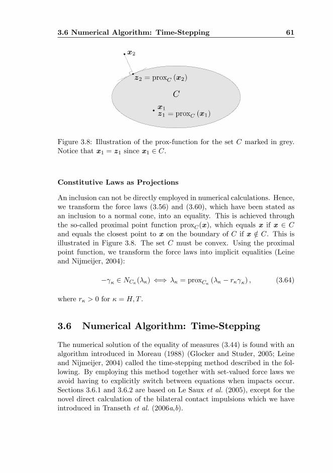
3.6 Numerical Algorithm: Time-Stepping 61
Figure 3.8: Illustration of the prox-function for the set C marked in grey.Notice that x1 = z1 since x1 2 C.
Constitutive Laws as Projections
An inclusion can not be directly employed in numerical calculations. Hence,we transform the force laws (3.56) and (3.60), which have been stated asan inclusion to a normal cone, into an equality. This is achieved throughthe so-called proximal point function proxC(x), which equals x if x 2 Cand equals the closest point to x on the boundary of C if x =2 C. This isillustrated in Figure 3.8. The set C must be convex. Using the proximalpoint function, we transform the force laws into implicit equalities (Leineand Nijmeijer, 2004):
� � 2 NC�(��) () �� = proxC� (�� � r� �) ; (3.64)
where r� > 0 for � = H;T .
3.6 Numerical Algorithm: Time-Stepping
The numerical solution of the equality of measures (3.44) is found with analgorithm introduced in Moreau (1988) (Glocker and Studer, 2005; Leineand Nijmeijer, 2004) called the time-stepping method described in the fol-lowing. By employing this method together with set-valued force laws weavoid having to explicitly switch between equations when impacts occur.Sections 3.6.1 and 3.6.2 are based on Le Saux et al. (2005), except for thenovel direct calculation of the bilateral contact impulsions which we haveintroduced in Transeth et al. (2006a,b).
62 Non-smooth Model of a 2D Snake Robot for Simulation
3.6.1 Time Discretization
Let tl denote the time at time-step l = 1; 2; 3; : : : where the step size is�t = tl+1 � tl. Consider the (usually very short) time interval It = [tA; tE ]and let tA = tl. De�ne qA = q(tA), uA = u(tA) which are admissiblewith respect to both the unilateral and bilateral constraints. Our goal isnow to �nd qE = q(tE)
1. We use the states of the system at the mid-point tM = tA +
12�t of the time-interval It to decide which contact points
are active (i.e. whether or not any links are touching an obstacle). Thecoordinates (positions and orientations) at tM are found from
qM = qA +�t
2uA: (3.65)
The approximation of the matrices W�, where � = H;T; J , on the time-interval It is given as W�M := W�(qM ). A numerical approximation ofthe equality of measures (3.44) over the time-interval It can now be writtenas
M (uE � uA)� S �WJM P J = ��t; (3.66)
where
S =Xb2HM
(WHM )b PHb +WTMP T ; (3.67)
and PHb , P T and P J are the contact impulsions during the time-interval It.They consist of forces � acting during It and possible impulses � acting inthe time-interval It. To �nd the positions and orientations qE at the end ofthe time-interval, we need to solve (3.66) for uE and the contact impulsions.The contact impulsions associated with obstacle and ground frictional con-tact are found using the prox-functions described in Section 3.5.2 for theset of active contact points HM found by (3.47) with t = tM . Hence, theconstitutive laws (3.64) for the obstacle contact and friction impulsions maynow be written as
PHb = proxCH�PHb � rH HEb
�; b 2 HM ; (3.68)
P Ta = proxCT�P Ta � rT TEa
�; a = 1; : : : ; n; (3.69)
1 In order to clarify the use of notation, we note that the subscript letters A and Erefer to the German words �Anfang�which means �beginning�, and �Ende�which means�end�.
3.6 Numerical Algorithm: Time-Stepping 63
where rH ; rT > 0, HEb is the b-th element of the vector HE , TEa is thevector of the (2a� 1)-th and 2a-th element of TE and
HE := H (qM ;uE) =WTHM uE ; (3.70)
TE := T (qM ;uE) =WTTM uE : (3.71)
The constitutive laws (3.68)-(3.71) are valid for completely inelastic im-pacts.
The constraints on the joints are bilateral and it therefore holds that
JE := J (qE ;uE) =WTJM uE = 0; 8t: (3.72)
This allows us to directly compute the associated contact impulsions P J
by employing (3.66) and (3.72):
P J = ��WT
JMM�1WJM
��1WT
JM
�uA +M
�1 (S + ��t)�: (3.73)
The equations (3.66)-(3.71) and (3.73) constitute a set of non-smooth equa-tions where the number of unknowns uE , PHb , P T and P J , equals the num-ber of equations. An algorithm to solve this set of equations is describedin Section 3.6.2. After having solved for uE we �nd the position at the endof the time-step as
qE = qM +�t
2uE : (3.74)
Notice from (3.66)-(3.74) that no explicit change between equationsare needed (when for example an impact between the snake robot andan obstacle occurs) since both the non-impulsive forces and the impactimpulses are covered by the same constitutive laws (3.68)-(3.69).
3.6.2 Solving for the Contact Impulsions
The numerical integration algorithm used in this chapter is called a time-stepping method which allows for a simultaneous treatment of both impul-sive and non-impulsive forces during a time-step. The frictional contactproblem, de�ned by (3.66)-(3.71) and (3.73), needs to be solved for eachtime-step tl. A Modi�ed Newton Algorithm (Alart and Curnier, 1991) hasbeen chosen, because of its simplicity, to solve the non-linear problem iter-atively. Let the superscript (k) denote the current iteration of the Modi�edNewton Algorithm and initialize all contact impulsions (for active contacts)with the value they had the last time their corresponding contact point wasactive. Now, the algorithm may be written as:
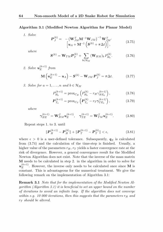
64 Non-smooth Model of a 2D Snake Robot for Simulation
Algorithm 3.1 (Modi�ed Newton Algorithm for Planar Model)
1. SolveP(k)J = �
�WT
JMM�1WJM
��1WT
JM �huA +M
�1�S(k) + ��t
�i;
(3.75)
whereS(k) =WTMP
(k)T +
Xb2HM
(WHM )b P(k)Hb: (3.76)
2. Solve u(k+1)E from
M�u(k+1)E � uA
�� S(k) �WJM P
(k)J = ��t: (3.77)
3. Solve for a = 1; : : : ; n and b 2 HM
P(k+1)Hb
= proxCH
�P(k)Hb� rH (k+1)HEb
�; (3.78)
P(k+1)Ta
= proxCT
�P(k)Ta� rT (k+1)TEa
�; (3.79)
where
(k+1)HE =WT
HMu(k+1)E ;
(k+1)TE =WT
TMu(k+1)E : (3.80)
Repeat steps 1. to 3. until
kP (k+1)H � P (k)
H k+ kP (k+1)T � P (k)
T k < �; (3.81)
where � > 0 is a user-de�ned tolerance. Subsequently, qE is calculatedfrom (3.74) and the calculation of the time-step is �nished. Usually, ahigher value of the parameters rH , rT yields a faster convergence rate at therisk of divergence. However, a general convergence result for the Modi�edNewton Algorithm does not exist. Note that the inverse of the mass matrixM needs to be calculated in step 2. in the algorithm in order to solve foru(k+1)E . However, the inverse only needs to be calculated once since M isconstant. This is advantageous for the numerical treatment. We give thefollowing remark on the implementation of Algorithm 3.1:
Remark 3.1 Note that for the implementation of the Modi�ed Newton Al-gorithm (Algorithm 3.1) it is bene�cial to set an upper bound on the numberof iterations to avoid an in�nite loop. If the algorithm does not convergewithin e.g. 10 000 iterations, then this suggests that the parameters rH andrT should be altered.
3.7 Summary 65
The constitutive laws (3.78)-(3.80) used to describe the contact impulsesare given on velocity level. This means that the bilateral constraints onposition level are in general not satis�ed. A solution to this problems issuggested in the following.
3.6.3 Constraint Violation
The contact impulses P J are calculated such that the bilateral constraintsare satis�ed on velocity level. In order to prevent that adjacent links driftapart, we project the positions of the links so that the bilateral constraintsare satis�ed on position level after the Modi�ed Newton Algorithm hasconverged and qE has been found from (3.74). The projection is performedby keeping the position of link 1 �xed together with the orientations ofall links. Then the links are moved so that all the gap functions (3.14)associated with the joints are equal to zero, i.e. gJi� = 0 for � = x; y andi = 1; : : : ; n � 1, and the vector qE is updated with the new positions ofthe links.
The projection performed to satisfy the bilateral constraints on positionlevel adds additional computations to the numerical treatment of the snakerobot model. An alternative approach is to reduce the number of gen-eralized coordinates (from a non-minimal description) by expressing thebilateral constraints analytically and then incorporating them implicitlyinto the model. However, some sort of projection algorithm will in somecases still be necessary to avoid that the links drift apart depending on thechoice of generalized coordinates and the accuracy of the numerical inte-grator. Another approach would be to develop the model from a set ofminimal coordinates directly, but then the system matrices will grow verylarge when the number of links is increased. With the modelling approachdescribed in this chapter, we avoid having to rewrite the model (from anon-minimal set of coordinates) to a new (minimal) set of coordinates andthe system matrices are kept simple. Hence, we have the positions of alllinks directly available and the appearance of the model makes it easy tounderstand. Moreover, it is less demanding to extend the model to 3Dwhere an implicit incorporation of the bilateral constraints in the modelwould prove cumbersome.
3.7 Summary
A novel mathematical 2D model based on the framework of non-smoothdynamics and convex analysis is developed for a snake robot in an envi-
66 Non-smooth Model of a 2D Snake Robot for Simulation
ronment with external objects in this chapter. The model describes planarsnake robot motion where the snake robot can push against external ob-stacles over the entire surface of each link. Hence, the e¤ect of the contactforces between the obstacle and each link is modelled properly and motionpatterns which are based on that the snake robot pushes against externalobjects can be tested with even very small objects. It has been shownhow to easily incorporate the normal contact and friction forces into thesystem dynamics (i.e. the equality of measures) by set-valued force laws.The modelling framework allowed for accurately describing rigid body con-tact and collisions in a hybrid manner without having to explicitly switchbetween system equations. Moreover, it has been shown how to includecorrect directional Coulomb friction. Hence, the model can be employedto simulate various planar motion patterns both with and without externalobjects to push against. In addition, the concise description of the modeland its numerical treatment give others the opportunity to implement themodel for simulation.
In addition to presenting the 2D model of the snake robot, this chapterserves as an introduction to the various modelling techniques in the frame-work of non-smooth dynamics and convex analysis that have been necessaryto employ in this thesis. In the following chapters, we will utilize and referto the general theory given in this chapter.
Chapter 4
3D Snake Robot Modellingfor Simulation
4.1 Introduction
Biological snakes may lift parts of their body during locomotion by a form oflateral undulation (called sinus-lifting) to move faster and more e¢ cient. Inaddition, snakes that travel on a surface with uniform friction may employa serpentine motion pattern called sidewinding for locomotion. Both ofthese motion patterns require that parts of the snake robot body are lifted.For this reason, a model of a snake robot capable of such motion patternsis needed to include the possibility of 3D motion.
In this chapter we extend the non-smooth 2D model given in Chap-ter 3 to 3D motion. We model the snake robot with 2 degrees of freedom(DOF) cardan joints and cylindrical links. The snake robot is set in anenvironment with vertical cylindrical obstacles that it may push againstfor locomotion. The general procedure for developing the model is similarto the development of the 2D model. However, di¤erent coordinates arechosen and additional constitutive laws need to be added (e.g. a varyingnormal force between the snake robot and the ground). The summary ofthe 2D model presented in Section 3.2 can be read as an introduction to thedevelopment of the 3D model also since the general approach is the same.
This chapter is based on Transeth et al. (2006a), Transeth et al. (2006b)and Transeth et al. (2008a) and it is organized as follows. The kinematicsof the snake robot with the ground surface as a unilateral constraint isdescribed in Section 4.2. Then the groundwork for �nding the friction andground contact forces is laid in Section 4.3. The non-smooth dynamics is
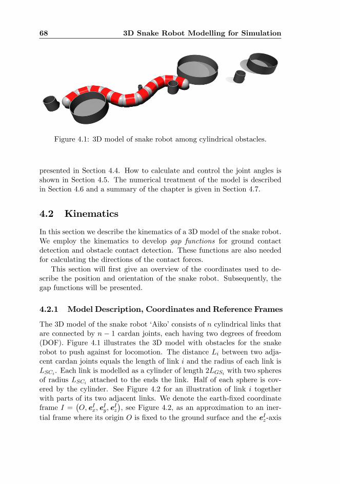
68 3D Snake Robot Modelling for Simulation
Figure 4.1: 3D model of snake robot among cylindrical obstacles.
presented in Section 4.4. How to calculate and control the joint angles isshown in Section 4.5. The numerical treatment of the model is describedin Section 4.6 and a summary of the chapter is given in Section 4.7.
4.2 Kinematics
In this section we describe the kinematics of a 3D model of the snake robot.We employ the kinematics to develop gap functions for ground contactdetection and obstacle contact detection. These functions are also neededfor calculating the directions of the contact forces.
This section will �rst give an overview of the coordinates used to de-scribe the position and orientation of the snake robot. Subsequently, thegap functions will be presented.
4.2.1 Model Description, Coordinates and Reference Frames
The 3D model of the snake robot �Aiko�consists of n cylindrical links thatare connected by n � 1 cardan joints, each having two degrees of freedom(DOF). Figure 4.1 illustrates the 3D model with obstacles for the snakerobot to push against for locomotion. The distance Li between two adja-cent cardan joints equals the length of link i and the radius of each link isLSCi . Each link is modelled as a cylinder of length 2LGSi with two spheresof radius LSCi attached to the ends the link. Half of each sphere is cov-ered by the cylinder. See Figure 4.2 for an illustration of link i togetherwith parts of its two adjacent links. We denote the earth-�xed coordinateframe I =
�O;eIx; e
Iy; e
Iz
�, see Figure 4.2, as an approximation to an iner-
tial frame where its origin O is �xed to the ground surface and the eIz-axis
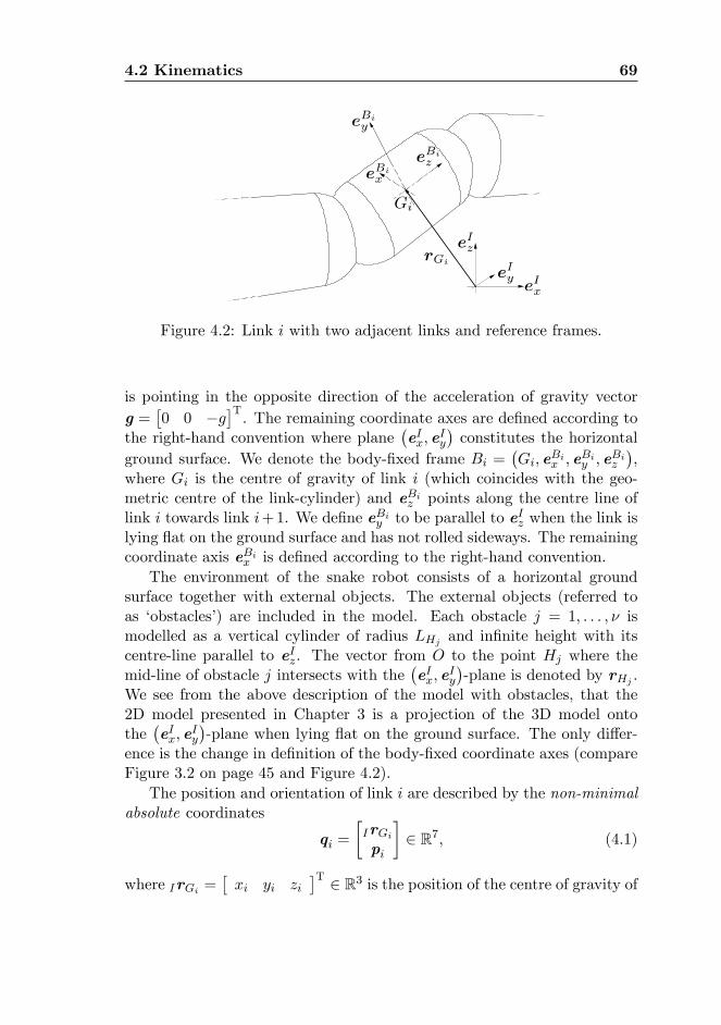
4.2 Kinematics 69
Figure 4.2: Link i with two adjacent links and reference frames.
is pointing in the opposite direction of the acceleration of gravity vectorg =
�0 0 �g
�T. The remaining coordinate axes are de�ned according to
the right-hand convention where plane�eIx; e
Iy
�constitutes the horizontal
ground surface. We denote the body-�xed frame Bi =�Gi; e
Bix ; e
Biy ; e
Biz
�,
where Gi is the centre of gravity of link i (which coincides with the geo-metric centre of the link-cylinder) and eBiz points along the centre line oflink i towards link i+1. We de�ne eBiy to be parallel to eIz when the link islying �at on the ground surface and has not rolled sideways. The remainingcoordinate axis eBix is de�ned according to the right-hand convention.
The environment of the snake robot consists of a horizontal groundsurface together with external objects. The external objects (referred toas �obstacles�) are included in the model. Each obstacle j = 1; : : : ; � ismodelled as a vertical cylinder of radius LHj and in�nite height with itscentre-line parallel to eIz. The vector from O to the point Hj where themid-line of obstacle j intersects with the
�eIx; e
Iy
�-plane is denoted by rHj .
We see from the above description of the model with obstacles, that the2D model presented in Chapter 3 is a projection of the 3D model ontothe
�eIx; e
Iy
�-plane when lying �at on the ground surface. The only di¤er-
ence is the change in de�nition of the body-�xed coordinate axes (compareFigure 3.2 on page 45 and Figure 4.2).
The position and orientation of link i are described by the non-minimalabsolute coordinates
qi =
�IrGipi
�2 R7; (4.1)
where IrGi =�xi yi zi
�T 2 R3 is the position of the centre of gravity of
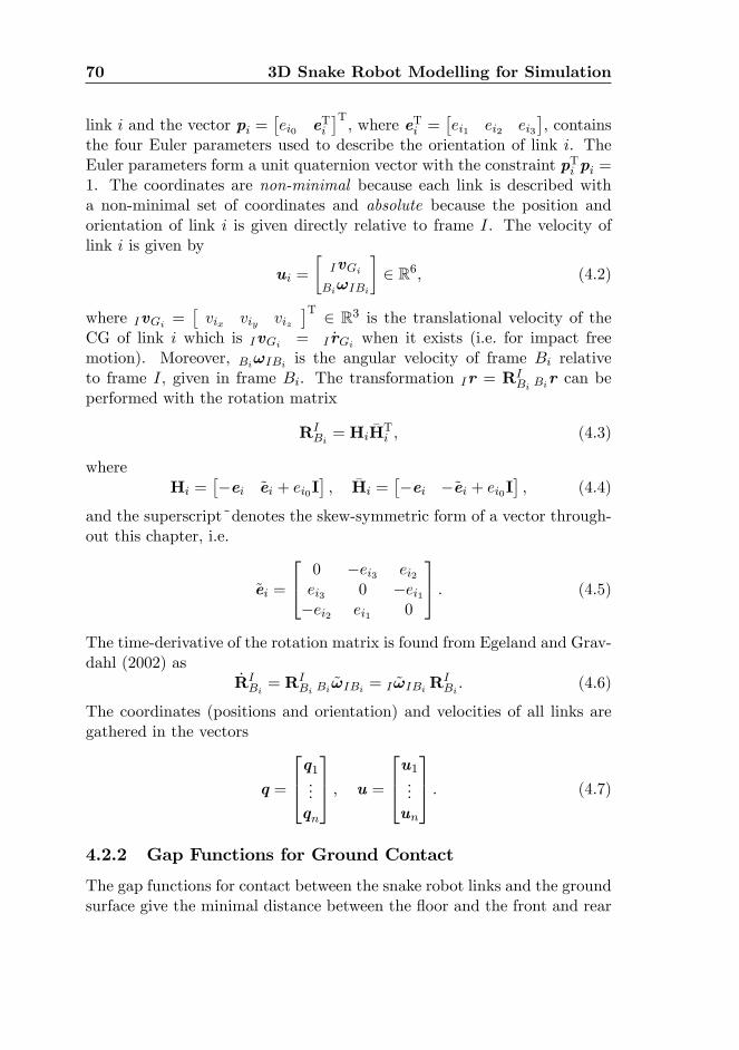
70 3D Snake Robot Modelling for Simulation
link i and the vector pi =�ei0 eTi
�T, where eTi =
�ei1 ei2 ei3
�, contains
the four Euler parameters used to describe the orientation of link i. TheEuler parameters form a unit quaternion vector with the constraint pTi pi =1. The coordinates are non-minimal because each link is described witha non-minimal set of coordinates and absolute because the position andorientation of link i is given directly relative to frame I. The velocity oflink i is given by
ui =
�IvGiBi!IBi
�2 R6; (4.2)
where IvGi =�vix viy viz
�T 2 R3 is the translational velocity of theCG of link i which is IvGi = I _rGi when it exists (i.e. for impact freemotion). Moreover, Bi!IBi is the angular velocity of frame Bi relativeto frame I, given in frame Bi. The transformation Ir = RI
Bi Bir can be
performed with the rotation matrix
RIBi = Hi
�HTi ; (4.3)
whereHi =
��ei ~ei + ei0I
�; �Hi =
��ei �~ei + ei0I
�; (4.4)
and the superscript~denotes the skew-symmetric form of a vector through-out this chapter, i.e.
~ei =
24 0 �ei3 ei2ei3 0 �ei1�ei2 ei1 0
35 : (4.5)
The time-derivative of the rotation matrix is found from Egeland and Grav-dahl (2002) as
_RIBi = R
IBi Bi
~!IBi = I ~!IBiRIBi : (4.6)
The coordinates (positions and orientation) and velocities of all links aregathered in the vectors
q =
264q1...qn
375 ; u =
264u1...un
375 : (4.7)
4.2.2 Gap Functions for Ground Contact
The gap functions for contact between the snake robot links and the groundsurface give the minimal distance between the �oor and the front and rear
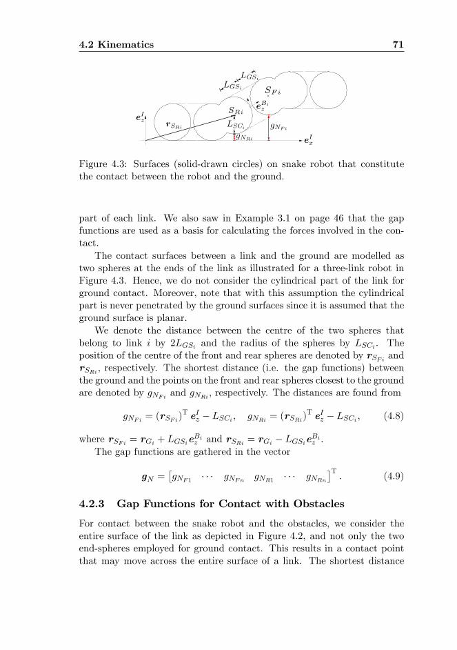
4.2 Kinematics 71
Figure 4.3: Surfaces (solid-drawn circles) on snake robot that constitutethe contact between the robot and the ground.
part of each link. We also saw in Example 3.1 on page 46 that the gapfunctions are used as a basis for calculating the forces involved in the con-tact.
The contact surfaces between a link and the ground are modelled astwo spheres at the ends of the link as illustrated for a three-link robot inFigure 4.3. Hence, we do not consider the cylindrical part of the link forground contact. Moreover, note that with this assumption the cylindricalpart is never penetrated by the ground surfaces since it is assumed that theground surface is planar.
We denote the distance between the centre of the two spheres thatbelong to link i by 2LGSi and the radius of the spheres by LSCi . Theposition of the centre of the front and rear spheres are denoted by rSFi andrSRi , respectively. The shortest distance (i.e. the gap functions) betweenthe ground and the points on the front and rear spheres closest to the groundare denoted by gNFi and gNRi , respectively. The distances are found from
gNFi = (rSFi)T eIz � LSCi ; gNRi = (rSRi)
T eIz � LSCi ; (4.8)
where rSFi = rGi + LGSieBiz and rSRi = rGi � LGSieBiz .
The gap functions are gathered in the vector
gN =�gNF1 � � � gNFn gNR1 � � � gNRn
�T: (4.9)
4.2.3 Gap Functions for Contact with Obstacles
For contact between the snake robot and the obstacles, we consider theentire surface of the link as depicted in Figure 4.2, and not only the twoend-spheres employed for ground contact. This results in a contact pointthat may move across the entire surface of a link. The shortest distance
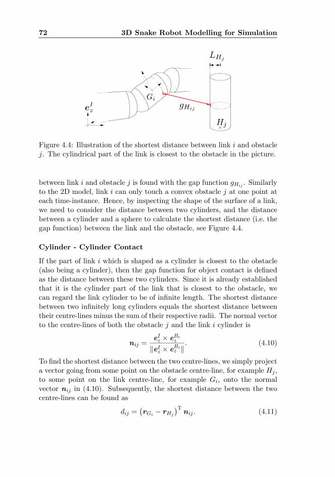
72 3D Snake Robot Modelling for Simulation
Figure 4.4: Illustration of the shortest distance between link i and obstaclej. The cylindrical part of the link is closest to the obstacle in the picture.
between link i and obstacle j is found with the gap function gHij . Similarlyto the 2D model, link i can only touch a convex obstacle j at one point ateach time-instance. Hence, by inspecting the shape of the surface of a link,we need to consider the distance between two cylinders, and the distancebetween a cylinder and a sphere to calculate the shortest distance (i.e. thegap function) between the link and the obstacle, see Figure 4.4.
Cylinder - Cylinder Contact
If the part of link i which is shaped as a cylinder is closest to the obstacle(also being a cylinder), then the gap function for object contact is de�nedas the distance between these two cylinders. Since it is already establishedthat it is the cylinder part of the link that is closest to the obstacle, wecan regard the link cylinder to be of in�nite length. The shortest distancebetween two in�nitely long cylinders equals the shortest distance betweentheir centre-lines minus the sum of their respective radii. The normal vectorto the centre-lines of both the obstacle j and the link i cylinder is
nij =eIz � eBizkeIz � eBiz k
: (4.10)
To �nd the shortest distance between the two centre-lines, we simply projecta vector going from some point on the obstacle centre-line, for example Hj ,to some point on the link centre-line, for example Gi, onto the normalvector nij in (4.10). Subsequently, the shortest distance between the twocentre-lines can be found as
dij =�rGi � rHj
�Tnij : (4.11)
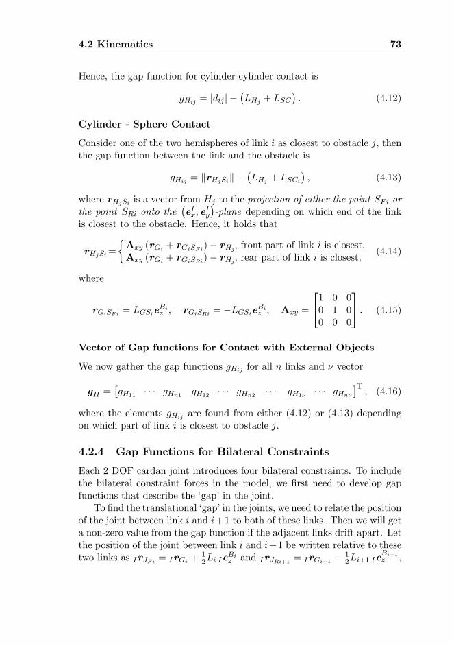
4.2 Kinematics 73
Hence, the gap function for cylinder-cylinder contact is
gHij = jdij j ��LHj + LSC
�: (4.12)
Cylinder - Sphere Contact
Consider one of the two hemispheres of link i as closest to obstacle j, thenthe gap function between the link and the obstacle is
gHij = krHjSik ��LHj + LSCi
�; (4.13)
where rHjSi is a vector from Hj to the projection of either the point SFi orthe point SRi onto the
�eIx; e
Iy
�-plane depending on which end of the link
is closest to the obstacle. Hence, it holds that
rHjSi=
�Axy (rGi + rGiSFi)� rHj, front part of link i is closest;Axy (rGi + rGiSRi)� rHj, rear part of link i is closest;
(4.14)
where
rGiSFi = LGSieBiz ; rGiSRi = �LGSieBiz ; Axy =
241 0 00 1 00 0 0
35 : (4.15)
Vector of Gap functions for Contact with External Objects
We now gather the gap functions gHij for all n links and � vector
gH =�gH11 � � � gHn1 gH12 � � � gHn2 � � � gH1� � � � gHn�
�T; (4.16)
where the elements gHij are found from either (4.12) or (4.13) dependingon which part of link i is closest to obstacle j.
4.2.4 Gap Functions for Bilateral Constraints
Each 2 DOF cardan joint introduces four bilateral constraints. To includethe bilateral constraint forces in the model, we �rst need to develop gapfunctions that describe the �gap�in the joint.
To �nd the translational �gap�in the joints, we need to relate the positionof the joint between link i and i+1 to both of these links. Then we will geta non-zero value from the gap function if the adjacent links drift apart. Letthe position of the joint between link i and i+1 be written relative to thesetwo links as IrJFi = IrGi +
12Li Ie
Biz and IrJRi+1 = IrGi+1 � 1
2Li+1 IeBi+1z ,
74 3D Snake Robot Modelling for Simulation
Figure 4.5: Illustration of how the translational gaps in the joint betweenlink i and link i+ 1 is found.
respectively. We see from Figure 4.5 that rJFi = rJRi+1when the twoadjacent links are in a position and orientation relative to each other thatis allowed by the cardan joint which connects the links. The gap functionsfor the translational gaps can now be found from
gJi� =�IrJFi � IrJRi+1
�TIeI�; (4.17)
for i = 1; : : : ; n� 1, and � = x; y; z. Hence, from (4.17) we found that
gJi� =�IrGi � IrGi+1
�TIeI�
+12
�LiR
IBi Bi
eBiz + Li+1RIBi+1 Bi+1
eBi+1z
�TIeI�;
(4.18)
for i = 1; : : : ; n� 1, and � = x; y; z.The next gap function provides the �gap� in rotation around the axis
that the cardan joint is not able to rotate around (one can only performpitch and yaw movement with a cardan joint and not roll). Let eBiy and
eBi+1x be the axes of rotation for the cardan joint between link i and linki+ 1, then �
eBiy�TeBi+1x = 0: (4.19)
Hence, a measure for the rotational �gap�can be de�ned from (4.19) as thegap function
gJi� =�RIBi Bie
Biy
�T �RIBi+1 Bi+1e
Bi+1x
�: (4.20)
4.3 Contact Constraints on Velocity Level 75
4.3 Contact Constraints on Velocity Level
In this section we calculate the relative velocities between the snake robotand the ground from the gap functions. The relative velocities are neededto set up the set-valued contact forces for the closed contacts (Le Saux etal., 2005).
4.3.1 Unilateral Contact: Ground Contact
Contact between the snake robot and the ground surface involves (verti-cal) normal forces, which guarantee the unilaterality of the contact, and(horizontal) tangential contact forces, which are due to friction and aredependent on the normal contact forces and the relative sliding velocities.We assumed that the normal contact forces between the snake robot andthe ground surface were constant in the 2D model in Chapter 3. For the3D model, this normal contact force is varying and we need to �nd thecorresponding relative velocities to calculate it.
Relative Velocities Along eIz
The relative velocities between the front and rear part of link i and theground along the eIz-axis are de�ned as NFi := _gNFi and NRi := _gNRi(when they exist), respectively, and they are used later to �nd the normalcontact forces. Before we proceed, note that NFi (or NRi) should not befound directly by taking the time-derivative of the expression for gNFi (orgNFi) in (4.8). This is the case since the expressions (4.8) have alreadybeen simpli�ed due to the fact that expressions have been inserted for thevarious body-�xed vectors which constitute the gap functions. Instead, forthe relative velocities, we must consider the velocity of the body-�xed pointPFi which at time-instant t coincides with the point CFi on the front sphereclosest to the ground (the same principle applies for the rear part of thelink). Note that the position vectors for PFi and CFi will be the sameinstantaneously. However, the di¤erentials will be di¤erent. This is shownin the following. Let CFi be a point on the front sphere that moves on thesphere such that the point is always closest to the ground surface. Thenthe position of this point is
rCFi = rGi + rGiSFi + rSFiCFi : (4.21)
76 3D Snake Robot Modelling for Simulation
The velocity of the point CFi is obtained by di¤erentiation of (4.21):
IvCFi = IvGi � ( I~rGiSFi + I~rSFiCFi)RIBi Bi!IBi| {z }
IvPFi
+RIBi Bi
_rSFiCFi ; (4.22)
where we now can use that
rSFiCFi = �LSCieIz; (4.23)
and we have employed (4.6) and Bi _rGiSFi = 0; together with the identitiesI ~!IBi IrGiSFi = � I!IBi I~rGiSFi and I ~!IBi IrSFiCFi = � I!IBi I~rSFiCFi .We see from (4.22) the expression for the velocity IvPFi of the body-�xedpoint PFi which at time-instance t coincides with the point CFi. Thisvelocity will be employed to �nd both the relative velocities along eIz andthe tangential relative velocities. The equivalent velocity IvPRi on the rearpart of the sphere is found similarly to IvPFi in (4.22) by replacing Fi byRi in (4.22)-(4.23).
Now, the relative velocities along eIz for the front and rear part of linki can be found as
NQi = ( IeIz)TIvPQi =) NQi = (wNQi)
Tui; (4.24)
where
wNQi =�(Ie
Iz)T �(IeIz)T
�I~rGiSQi + I~rSQiCQi
�RIBi
�T; (4.25)
for Q = F;R with rGiSFi = LGSi eBiz and rGiSRi = �LGSi eBiz . The moti-
vation to use the form (4.24) is that wNQi gives the generalized directionof the contact force between the ground and the front and rear part of linki.
A vector gathering all NFi and NRi is
N =WTNu; (4.26)
where
N =� NF1 : : : NFn NR1 : : : NRn
�T; (4.27)
WN =�WNF WNR
�2 R6n�2n; (4.28)
and
WNQ =
266664wNQ1 06�1 � � � 06�1
06�1. . .
......
. . . 06�106�1 � � � 06�1 wNQn
377775 2 R6n�n; (4.29)
for Q = F;R.
4.3 Contact Constraints on Velocity Level 77
Tangential Relative Velocities
The friction forces between a link and the ground depend on the relative ve-locities in the (eIx; e
Iy)-plane between the snake robot links and the ground.
These velocities are termed tangential relative velocities. First, the relativevelocities between the front part of link i and the ground along the eIx-and eIy-axis,
0TFix
and 0TFiy , will be deducted. Subsequently, the relativevelocities for the front part of link i along the projection of the longitudinalaxis of the link onto the (eIx; e
Iy)-plane TFix and transversal to the link
TFiy , will be deducted from 0TFix and 0TFiy
respectively. The same typeof notation applies for the rear part of link i: 0TRix ,
0TRiy
, TRix and TRiy .The tangential relative velocities are found much in the same way as for NFi and NRi . Consequently, we �nd the velocities of the points PFi andPRi along the eIx- and e
Iy-axis. Hence, by looking at (4.24), we see that the
tangential relative velocities of the contact points on the front part of thelink can be found as
0TFi� = (IeI�)TIvPFi =) 0TFi� = (w
0TFi�
)Tui; (4.30)
for � = x; y, where
w0TFi� =�(Ie
I�)T �(IeI�)T ( I~rGiSFi + I~rSFiCFi)R
IBi
�T: (4.31)
The relative velocities between the rear part of the link and the groundare found by exchanging IvPFi with IvPRi in (4.30):
0TRi� = (IeI�)TIvPRi =) 0TRi� = (w
0TRi�
)Tui; (4.32)
for � = x; y, where
w0TRi� =�(Ie
I�)T �(IeI�)T ( I~rGiSRi +I ~rSRiCRi)RI
Bi
�T: (4.33)
The tangential relative velocities for the front and rear part of the link iare combined in vectors:
0TQi =W0TTQiui; (4.34)
for Q = F;R, where 0TQi =h 0TQix 0TQiy
iTand
W0TQi
=hw0TQix w0TQiy
i2 R6�2: (4.35)
Until now the relative velocities have been given in the directions along theeIx and e
Iy axes. In order to calculate the friction forces longitudinal and
78 3D Snake Robot Modelling for Simulation
transversal to a link, we need to know the corresponding relative velocitiesin these directions in the
�eIx; e
Iy
�-plane. To calculate these velocities we
introduce for each link a frame �i with axes�e�ix ; e
�iy ; e
�iz
�, where Ie�iz =
IeIz, and
Ie�ix =
Axy IeBiz
kAxy IeBiz k
; Ie�iy =
IeIz � Ie
�ix
k IeIz � Ie�ix k
; (4.36)
where Axy = diag([1; 1; 0]). Hence, it holds that
RI�i =
�Ie�ix Ie
�iy Ie
�iz
�: (4.37)
Notice that Ie�ix = IeBiz and Ie
�iy = Ie
Bix when link i is lying �at on the
ground with IeBiy = Ie
Iz. Since only the motion in the
�eIx; e
Iy
�-plane is of
interest, we de�ne
�RI�i = D
TRI�iD; D =
�1 0 00 1 0
�T: (4.38)
Since we now have that 0TQi =�RI�i TQi , Q = F; R, the relative velocity
between the �oor and the front part of link i, with respect to frame �i, canbe found from (4.34) as
TQi =WTTQiui; (4.39)
where TQi =h TQix TQiy
iT; WTQi = W0
TQi�RI�i; for Q = F;R.
A vector that gathers all TFi and TRi is found from
T =WTTu; (4.40)
where
T =
2666666664
TF1...
TFn TR1...
TRn
37777777752 R4n; WT =
�WTF WTR
�2 R6n�4n; (4.41)
and
WTQ =
266664WTQ1 06�2 � � � 06�2
06�2. . .
......
. . . 06�206�2 � � � 06�2 WTQn
377775 2 R6n�2n; for Q = F;R: (4.42)
4.3 Contact Constraints on Velocity Level 79
Relative Rolling Velocities
Up until now we have only considered translational relative motion of thesnake robot links. However, we also need to consider rotational relativemotion to add a damping e¤ect on the rotational motion in the form ofrotational friction. In order to do this, we introduce the relative rollingvelocity as
VQi = DT �
IrCQiSQi � I!IBi�; (4.43)
for Q = F;R, where VQi =h VQix VQiy
iT, IrCQiSQi = LSCi Ie
Iz is the
vector pointing (upward) from the contact point point CQi on the link end-sphere closest to the ground, toward the centre SQi of the end-sphere andD is given in (4.38). By employing the identity
IrCQiSQi � I!IBi = I~rCQiSQiRIBiBi!IBi ;
we �nd that the relative rolling velocity can be written
VQi =WTVQiui; (4.44)
where
WTVQi
=�O2�3 DT
I~rCQiSQiRIBi
�; (4.45)
for Q = F;R.We gather all the relative rolling velocities as
V =WV u; (4.46)
where
V =
2666666664
VF1...
VFn VR1...
VRn
37777777752 R4n; WV =
�WVF WVR
�2 R6n�4n; (4.47)
andWVF ,WVR are found similarly to (4.42) by replacingWTFi andWTRi
in (4.42) byWVFi andWVRi , respectively.
80 3D Snake Robot Modelling for Simulation
4.3.2 Unilateral Contact: Obstacle Contact
Contact between link i and obstacle j is modelled as a unilateral contact.To calculate the contact force involved in the contact, the relative velocity Hij := _gHij between obstacle j and the point on link i closest to theobstacle needs to be found. This is obtained from the gap functions de�nedin Section 4.2.3. Equivalently to the calculations of the gap functions, therelative velocity Hij is dependent on which part of the link is closest tothe obstacle.
Cylinder - Cylinder Contact
If the cylinder part of link i is closest to obstacle j, then the gap functionis given by (4.12) and the relative velocity Hij := _gHij can be written as
Hij =�IvTGinij +
�rGi � rHj
�T_nij
�sign(dij); (4.48)
where nij and dij are found from (4.10) and (4.11), respectively. De�nek � k := k � k2 and consider
I _nij = �ddtkIe
Iz � Ie
Biz k
kIeIz � IeBiz k2
�IeIz � Ie
Biz
�+
ddt
�IeIz � Ie
Biz
�kIeIz � Ie
Biz k
; (4.49)
whereddt
�IeIz � Ie
Biz
�= �I~eIzRI
BiBi~eBiz Bi!IBi ; (4.50)
ddtkIeIz � Ie
Biz k =
��IeBiz
�TAxyR
IBiBi
~eBiz Bi!IBi
kIeIz � IeBiz k
; (4.51)
and ~eIz denotes the skew-symmetric form of eIz similarly to (4.5) on page 70.
Substitution of (4.49)-(4.51) into (4.48) yields
Hij = wTHijui; (4.52)
where
wHij = sign(dij) �h(Inij)
T cTijRIBiBi
~eBiz
iT; (4.53)
and
cTij =
�IrGi � IrHj
�TkIeIz � Ie
Biz k
Inij
�IeBiz
�TAxy
kIeIz � IeBiz k
� I~eIz
!: (4.54)
The motivation to write the relative velocity in the form (4.52) is that thevector wHij 2 R6 constitutes the generalized force direction of the contactforce between obstacle j and link i.
4.3 Contact Constraints on Velocity Level 81
Cylinder - Sphere Contact
The gap function in (4.13) is employed to de�ne the relative velocity Hij :=_gHij when one of the two hemispheres on link i is closest to the obstacle j.In order to �nd Hij , consider the vector IrHjSi in (4.14) which is a vectorfrom Hj to the projection of either the point SFi or the point SRi onto the�eIx; e
Iy
�-plane depending on which end of the link is closest to the obstacle.
The time-derivative of IrHjSi is
I _rHjSi = Axy
�IvGi �AxyR
IBi Bi
~rGiSi Bi!IBi�;
where Bi~rGiSi denotes the skew-symmetric form of BirGiSi and
rGiSi =
�rGiSFi , front part of link i is closest,rGiSRi , rear part of link i is closest.
(4.55)
We now �nd the relative velocity between obstacle j and the point closestto the obstacle on the front or rear sphere of link i as
Hij = wTHijui; (4.56)
where
wTHij =IrTHjSi
kIrHjSik�Axy �AxyR
IBi Bi
~rGiSi�: (4.57)
Vector of Relative Velocities for the Obstacle Contact
We now gather the relative velocities Hij for all n links and � obstacles inthe vector
H =WTHu; (4.58)
where
H =� H11 � � � Hn1 H12 � � � Hn2 � � � H1� � � � Hn�
�T; (4.59)
WH =�WH1 � � � WH�
�2 R6n�n� ; (4.60)
and
WHj =
266664wH1j 06�1 � � � 06�1
06�1. . .
......
. . . 06�106�1 � � � 06�1 wHnj
377775 2 R6n�n: (4.61)
Depending on which part of the link is closest to the obstacle, wHij isobtained from either (4.53) or (4.57).
82 3D Snake Robot Modelling for Simulation
4.3.3 Bilateral Constraints: Joints
The bilateral constraints introduced by the cardan joint between two ad-jacent links prohibit relative motion between the links in four DOF. Therelative velocities between the links along these DOF need to be found inorder to calculate the bilateral constraint forces in the joints. These relativevelocities are found from the gap functions gJi� , � = x; y; z, in (4.18) andgJi� in (4.20) for i = 1; : : : ; n� 1.
The relative velocities for the translational gap between link i and linki + 1 are de�ned as Ji� := _gJi� for i = 1; : : : ; n � 1 where � = x; y; z. Byemploying (4.18), we �nd that
Ji� = wTJi�
�uiui+1
�; (4.62)
where
wJi� =
2666664(Ie
I�)
��(Ie
I�)T Li2 R
IBi Bi
~eBiz
�T�(IeI�)
��(Ie
I�)T Li+1
2 RIBi+1 Bi+1
~eBi+1z
�T
3777775 : (4.63)
The relative velocity for the rotational gap is de�ned as Ji� := _gJi� fori = 1; : : : ; n� 1. Thus,
Ji� = wTJi�
�uiui+1
�; (4.64)
where
wJi� =
26666403�1
��RIBi Bi
~eBiy�T �
RIBi+1 Bi+1
eBi+1x
�03�1
��RIBi+1 Bi+1
~eBi+1x
�T �RIBi Bi
eBiy�377775 : (4.65)
Let Ji =h Jix Jiy Jiz Ji�
iT2 R4, then we can gather all the rela-
tive velocities concerned with the bilateral constraints in one vector
J =WTJu; (4.66)
4.4 Non-smooth Dynamics 83
where
J =
264 J1...
Jn�1
375 2 R4(n�1); (4.67)
WJ =
266664WT
J1 04�6 � � � 04�6
04�6 WTJ2
......
. . . 04�604�6 � � � 04�6 WT
Jn�1
377775T
2 R6n�4(n�1); (4.68)
andWJi =�wJix wJiy wJiz wJi�
�2 R12�4 for i = 1; : : : ; n� 1.
4.4 Non-smooth Dynamics
In this section we �rst present the various components of the equality ofmeasures for the 3D model. The equality of measures describes the dynam-ics of the snake robot as seen in Section 3.5.
4.4.1 The Equality of Measures
Consider the generalized velocity to be a function t 7! u(t) of locallybounded variation on a time-interval It = [tA; tE ] (Moreau, 1988). Thevelocity function u (t) and its di¤erential measure du for the 3D modelhave the same properties as the same function elaborated on for the 2Dmodel in Section 3.5.1. The only di¤erence is that the velocity function forthe 2D model describes, of course, the velocity of the links in the 2D model,while the velocity function in this chapter describes the velocities in the 3Dmodel.
The equality of measures (3.43) on page 54 is written for the 3D modelof the snake robot as
Mdu� h (u) dt� dR = �dt; (4.69)
where the mass matrix M, the vector of smooth forces h (u), the forcemeasure of possibly atomic impact impulsions dR and the vector of ap-plied torques � will be described in the following. Note that the di¤erentialmeasure du describes both the continuous change and possible discontinu-ities of the velocity u (see Section 3.5.1).
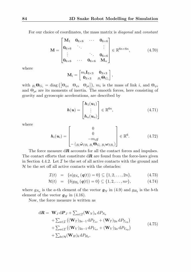
84 3D Snake Robot Modelling for Simulation
For our choice of coordinates, the mass matrix is diagonal and constant
M =
266664M1 06�6 � � � 06�6
06�6. . .
......
. . . 06�606�6 � � � 06�6 Mn
377775 2 R6n�6n; (4.70)
where
Mi =
�miI3�3 03�303�3 Bi�Gi
�;
with Bi�Gi = diag��� i � i ��i
��, mi is the mass of link i, and � i
and ��i are its moments of inertia. The smooth forces, here consisting ofgravity and gyroscopic accelerations, are described by
h(u) =
264h1(u1)...hn(un)
375 2 R6n; (4.71)
where
hi(ui) =
266400
�mig� (Bi ~!IBi Bi�Gi Bi!IBi)
3775 2 R6: (4.72)
The force measure dR accounts for all the contact forces and impulses.The contact e¤orts that constitute dR are found from the force-laws givenin Section 4.4.2. Let I be the set of all active contacts with the ground andH be the set o¤ all active contacts with the obstacles:
I(t) = fajgNa (q(t)) = 0g � f1; 2; : : : ; 2ng; (4.73)
H(t) = fbjgHb (q(t)) = 0g � f1; 2; : : : ; n�g; (4.74)
where gNa is the a-th element of the vector gN in (4.9) and gHb is the b-thelement of the vector gH in (4.16).
Now, the force measure is written as
dR = WJ dP J +P
a2I(WN )a dPNa
+P
a2I�(WT )2a�1 dPTax + (WT )2a dPTay
�+P
a2I�(WV )2a�1 dPVax + (WV )2a dPVay
�+P
b2H(WH)b dPHb ;
(4.75)
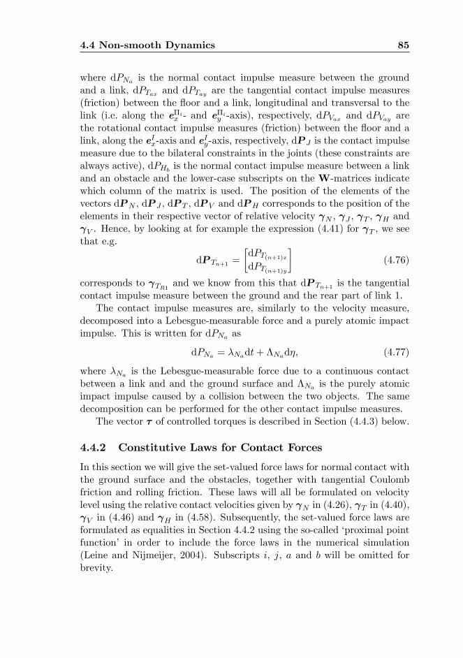
4.4 Non-smooth Dynamics 85
where dPNa is the normal contact impulse measure between the groundand a link, dPTax and dPTay are the tangential contact impulse measures(friction) between the �oor and a link, longitudinal and transversal to thelink (i.e. along the e�ix - and e
�iy -axis), respectively, dPVax and dPVay are
the rotational contact impulse measures (friction) between the �oor and alink, along the eIx-axis and e
Iy-axis, respectively, dP J is the contact impulse
measure due to the bilateral constraints in the joints (these constraints arealways active), dPHb is the normal contact impulse measure between a linkand an obstacle and the lower-case subscripts on theW-matrices indicatewhich column of the matrix is used. The position of the elements of thevectors dPN , dP J , dP T , dP V and dPH corresponds to the position of theelements in their respective vector of relative velocity N , J , T , H and V . Hence, by looking at for example the expression (4.41) for T , we seethat e.g.
dP Tn+1 =
�dPT(n+1)xdPT(n+1)y
�(4.76)
corresponds to TR1 and we know from this that dP Tn+1 is the tangentialcontact impulse measure between the ground and the rear part of link 1.
The contact impulse measures are, similarly to the velocity measure,decomposed into a Lebesgue-measurable force and a purely atomic impactimpulse. This is written for dPNa as
dPNa = �Nadt+ �Nad�; (4.77)
where �Na is the Lebesgue-measurable force due to a continuous contactbetween a link and and the ground surface and �Na is the purely atomicimpact impulse caused by a collision between the two objects. The samedecomposition can be performed for the other contact impulse measures.
The vector � of controlled torques is described in Section (4.4.3) below.
4.4.2 Constitutive Laws for Contact Forces
In this section we will give the set-valued force laws for normal contact withthe ground surface and the obstacles, together with tangential Coulombfriction and rolling friction. These laws will all be formulated on velocitylevel using the relative contact velocities given by N in (4.26), T in (4.40), V in (4.46) and H in (4.58). Subsequently, the set-valued force laws areformulated as equalities in Section 4.4.2 using the so-called �proximal pointfunction� in order to include the force laws in the numerical simulation(Leine and Nijmeijer, 2004). Subscripts i, j, a and b will be omitted forbrevity.
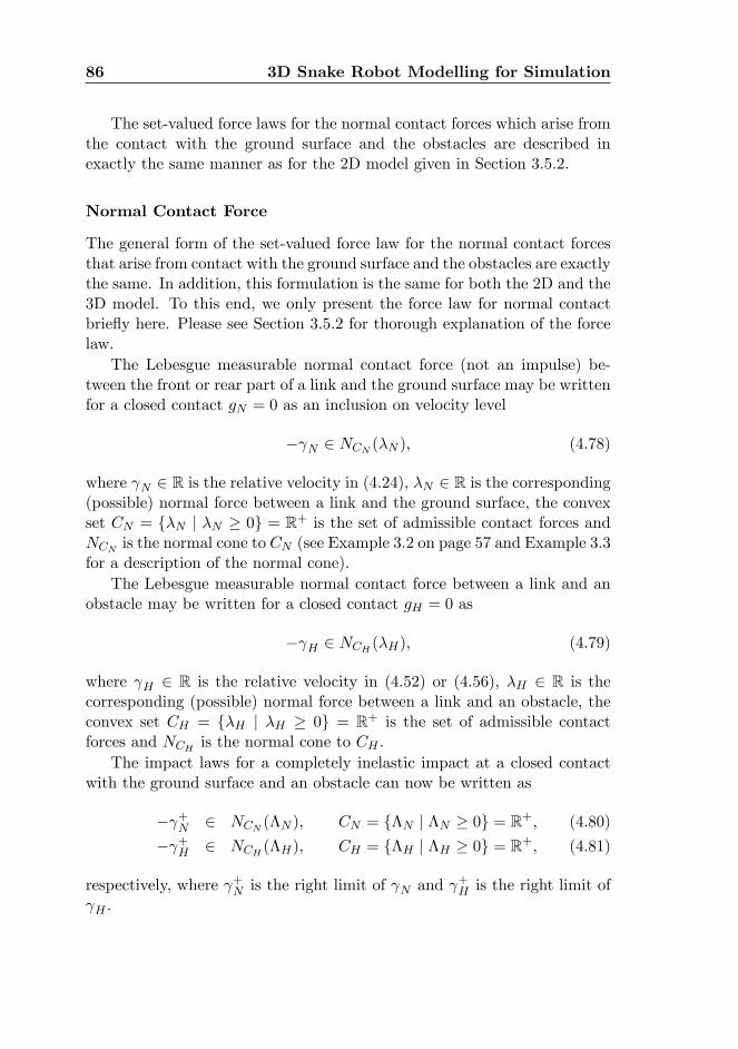
86 3D Snake Robot Modelling for Simulation
The set-valued force laws for the normal contact forces which arise fromthe contact with the ground surface and the obstacles are described inexactly the same manner as for the 2D model given in Section 3.5.2.
Normal Contact Force
The general form of the set-valued force law for the normal contact forcesthat arise from contact with the ground surface and the obstacles are exactlythe same. In addition, this formulation is the same for both the 2D and the3D model. To this end, we only present the force law for normal contactbrie�y here. Please see Section 3.5.2 for thorough explanation of the forcelaw.
The Lebesgue measurable normal contact force (not an impulse) be-tween the front or rear part of a link and the ground surface may be writtenfor a closed contact gN = 0 as an inclusion on velocity level
� N 2 NCN (�N ); (4.78)
where N 2 R is the relative velocity in (4.24), �N 2 R is the corresponding(possible) normal force between a link and the ground surface, the convexset CN = f�N j �N � 0g = R+ is the set of admissible contact forces andNCN is the normal cone to CN (see Example 3.2 on page 57 and Example 3.3for a description of the normal cone).
The Lebesgue measurable normal contact force between a link and anobstacle may be written for a closed contact gH = 0 as
� H 2 NCH (�H); (4.79)
where H 2 R is the relative velocity in (4.52) or (4.56), �H 2 R is thecorresponding (possible) normal force between a link and an obstacle, theconvex set CH = f�H j �H � 0g = R+ is the set of admissible contactforces and NCH is the normal cone to CH .
The impact laws for a completely inelastic impact at a closed contactwith the ground surface and an obstacle can now be written as
� +N 2 NCN (�N ); CN = f�N j �N � 0g = R+; (4.80)
� +H 2 NCH (�H); CH = f�H j �H � 0g = R+; (4.81)
respectively, where +N is the right limit of N and +H is the right limit of H .
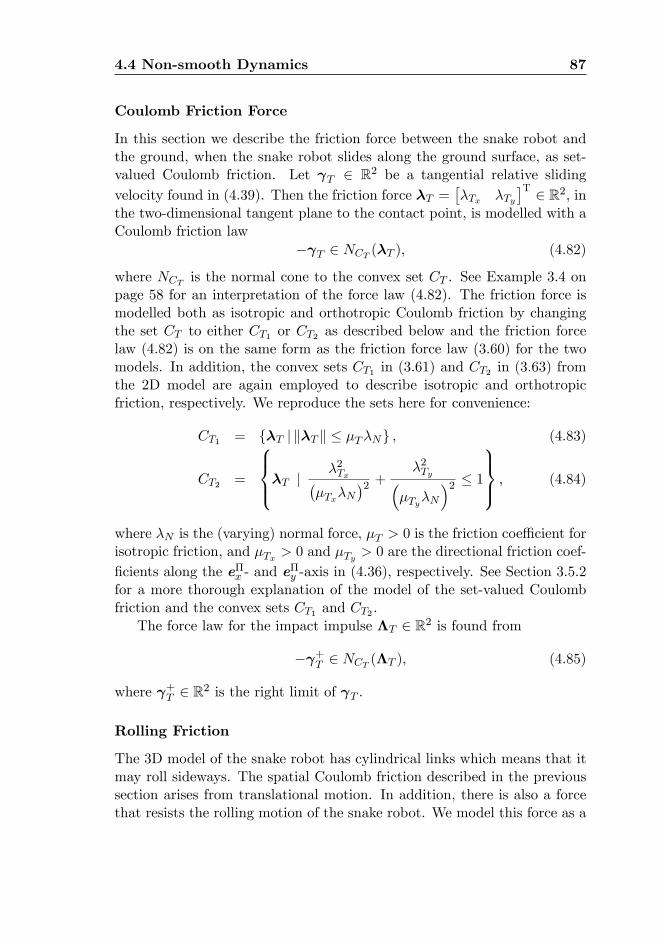
4.4 Non-smooth Dynamics 87
Coulomb Friction Force
In this section we describe the friction force between the snake robot andthe ground, when the snake robot slides along the ground surface, as set-valued Coulomb friction. Let T 2 R2 be a tangential relative slidingvelocity found in (4.39). Then the friction force �T =
��Tx �Ty
�T 2 R2, inthe two-dimensional tangent plane to the contact point, is modelled with aCoulomb friction law
� T 2 NCT (�T ); (4.82)
where NCT is the normal cone to the convex set CT . See Example 3.4 onpage 58 for an interpretation of the force law (4.82). The friction force ismodelled both as isotropic and orthotropic Coulomb friction by changingthe set CT to either CT1 or CT2 as described below and the friction forcelaw (4.82) is on the same form as the friction force law (3.60) for the twomodels. In addition, the convex sets CT1 in (3.61) and CT2 in (3.63) fromthe 2D model are again employed to describe isotropic and orthotropicfriction, respectively. We reproduce the sets here for convenience:
CT1 = f�T j k�T k � �T�Ng ; (4.83)
CT2 =
8><>:�T j �2Tx��Tx�N
�2 + �2Ty��Ty�N
�2 � 19>=>; ; (4.84)
where �N is the (varying) normal force, �T > 0 is the friction coe¢ cient forisotropic friction, and �Tx > 0 and �Ty > 0 are the directional friction coef-�cients along the e�x - and e
�y -axis in (4.36), respectively. See Section 3.5.2
for a more thorough explanation of the model of the set-valued Coulombfriction and the convex sets CT1 and CT2 .
The force law for the impact impulse �T 2 R2 is found from
� +T 2 NCT (�T ); (4.85)
where +T 2 R2 is the right limit of T .
Rolling Friction
The 3D model of the snake robot has cylindrical links which means that itmay roll sideways. The spatial Coulomb friction described in the previoussection arises from translational motion. In addition, there is also a forcethat resists the rolling motion of the snake robot. We model this force as a
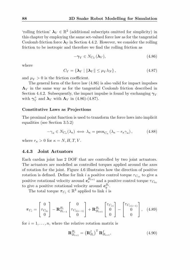
88 3D Snake Robot Modelling for Simulation
�rolling friction��V 2 R2 (additional subscripts omitted for simplicity) inthis chapter by employing the same set-valued force law as for the tangentialCoulomb friction force �T in Section 4.4.2. However, we consider the rollingfriction to be isotropic and therefore we �nd the rolling friction as
� V 2 NCV (�V ); (4.86)
whereCV = f�V j k�V k � �V �Ng ; (4.87)
and �V > 0 is the friction coe¢ cient.The general form of the force law (4.86) is also valid for impact impulses
�V in the same way as for the tangential Coulomb friction described inSection 4.4.2. Subsequently, the impact impulse is found by exchanging Vwith +V and �V with �V in (4.86)-(4.87).
Constitutive Laws as Projections
The proximal point function is used to transform the force laws into implicitequalities (see Section 3.5.2)
� � 2 NC�(��) () �� = proxC� (�� � r� �) ; (4.88)
where r� > 0 for � = N;H; T; V .
4.4.3 Joint Actuators
Each cardan joint has 2 DOF that are controlled by two joint actuators.The actuators are modelled as controlled torques applied around the axesof rotation for the joint. Figure 4.6 illustrates how the direction of positiverotation is de�ned. De�ne for link i a positive control torque �Cvi to give apositive rotational velocity around eBi+1x and a positive control torque �Chito give a positive rotational velocity around eBiy .
The total torque �Ci 2 R3 applied to link i is
�Ci =
24 0�Chi0
35�RBiBi�1
24 0�Ch(i�1)0
35+RBiBi+1
24�Cvi00
35�24�Cv(i�1)0
0
35 ; (4.89)
for i = 1; : : : ; n, where the relative rotation matrix is
RBiBi+1
=�RIBi
�TRIBi+1 ; (4.90)
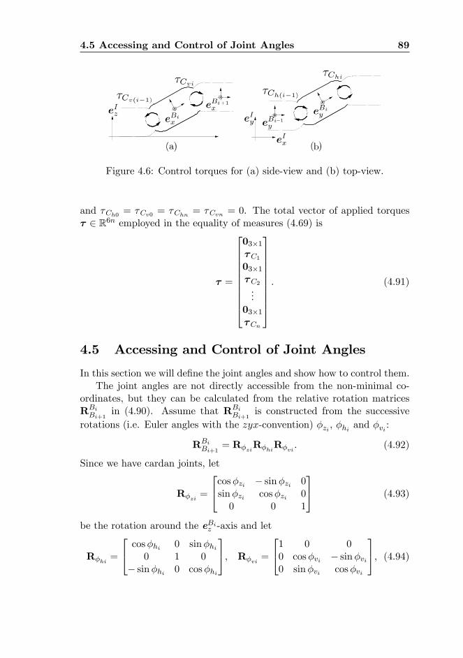
4.5 Accessing and Control of Joint Angles 89
Figure 4.6: Control torques for (a) side-view and (b) top-view.
and �Ch0 = �Cv0 = �Chn = �Cvn = 0. The total vector of applied torques� 2 R6n employed in the equality of measures (4.69) is
� =
26666666664
03�1�C103�1�C2...
03�1�Cn
37777777775: (4.91)
4.5 Accessing and Control of Joint Angles
In this section we will de�ne the joint angles and show how to control them.The joint angles are not directly accessible from the non-minimal co-
ordinates, but they can be calculated from the relative rotation matricesRBiBi+1
in (4.90). Assume that RBiBi+1
is constructed from the successiverotations (i.e. Euler angles with the zyx-convention) �zi , �hi and �vi :
RBiBi+1
= R�ziR�hiR�vi : (4.92)
Since we have cardan joints, let
R�zi =
24cos�zi � sin�zi 0sin�zi cos�zi 00 0 1
35 (4.93)
be the rotation around the eBiz -axis and let
R�hi =
24 cos�hi 0 sin�hi0 1 0
� sin�hi 0 cos�hi
35; R�vi =
241 0 00 cos�vi � sin�vi0 sin�vi cos�vi
35; (4.94)
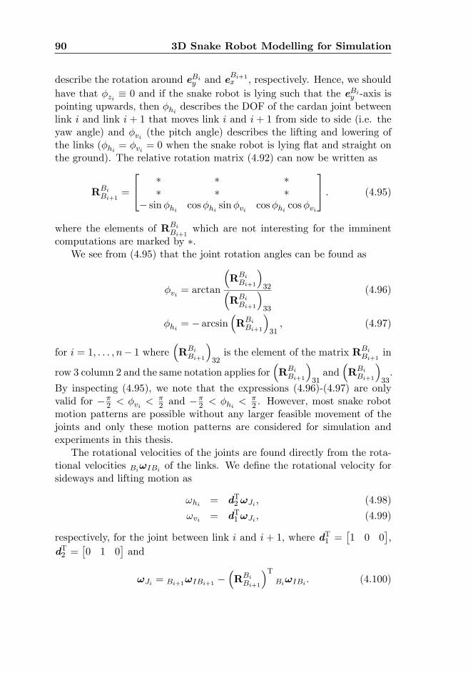
90 3D Snake Robot Modelling for Simulation
describe the rotation around eBiy and eBi+1x , respectively. Hence, we shouldhave that �zi � 0 and if the snake robot is lying such that the e
Biy -axis is
pointing upwards, then �hi describes the DOF of the cardan joint betweenlink i and link i+ 1 that moves link i and i+ 1 from side to side (i.e. theyaw angle) and �vi (the pitch angle) describes the lifting and lowering ofthe links (�hi = �vi = 0 when the snake robot is lying �at and straight onthe ground). The relative rotation matrix (4.92) can now be written as
RBiBi+1
=
24 � � �� � �
� sin�hi cos�hi sin�vi cos�hi cos�vi
35 : (4.95)
where the elements of RBiBi+1
which are not interesting for the imminentcomputations are marked by �.
We see from (4.95) that the joint rotation angles can be found as
�vi = arctan
�RBiBi+1
�32�
RBiBi+1
�33
(4.96)
�hi = � arcsin�RBiBi+1
�31; (4.97)
for i = 1; : : : ; n� 1 where�RBiBi+1
�32is the element of the matrix RBi
Bi+1in
row 3 column 2 and the same notation applies for�RBiBi+1
�31and
�RBiBi+1
�33.
By inspecting (4.95), we note that the expressions (4.96)-(4.97) are onlyvalid for ��
2 < �vi <�2 and �
�2 < �hi <
�2 . However, most snake robot
motion patterns are possible without any larger feasible movement of thejoints and only these motion patterns are considered for simulation andexperiments in this thesis.
The rotational velocities of the joints are found directly from the rota-tional velocities Bi!IBi of the links. We de�ne the rotational velocity forsideways and lifting motion as
!hi = dT2 !Ji ; (4.98)
!vi = dT1 !Ji ; (4.99)
respectively, for the joint between link i and i + 1, where dT1 =�1 0 0
�,
dT2 =�0 1 0
�and
!Ji = Bi+1!IBi+1 ��RBiBi+1
�TBi!IBi : (4.100)
4.6 Numerical Algorithm: Time-stepping 91
Let the desired values of �hi and �vi be �hi;d and �vi;d, respectively.In addition, the reference values for the joint velocities !hi , !vi are givenby _�hi;d and
_�vi;d, respectively. Then the torques applied to the joints arefound by PD-controllers as
�Chi = �kP��hi;d � �hi
�� kD
�_�hi;d � !hi
�; (4.101)
�Cvi = �kP��vi;d � �vi
�� kD
�_�vi;d � !vi
�; (4.102)
for i = 1; : : : ; n � 1 where kP 2 R+; kD 2 R+ are positive constants equalfor all i.
4.6 Numerical Algorithm: Time-stepping
In this section we will present the time-stepping method as the numericalsolution of the equality of measures for the 3D model of the snake robot.The general form of the algorithm is similar to that presented for the 2Dmodel in Chapter 3. However, the non-minimal coordinates are found witha di¤erent function and more contact impulse measures are added, bothsince we are now dealing with a 3D model instead of a planar one.
4.6.1 Time Discretization
The time discretization of the equality of measures for the 2D model isshown in Section 3.6 and the general approach is the same for the 3D model.Therefore, for the 3D model, we will only state a concise algorithm thatconstitutes the time-stepping method for the 3D model. An elaboration onthis procedure is found in Section 3.6. In the following, we will describethe time-stepping algorithm for the 3D model.
The mid-point qM in the time-stepping method for the 3D model isfound from
qM = qA +�t
2F(qA)uA (4.103)
where we have used the equality _p = 12�HT
Bi!IBi (Egeland and Gravdahl,2002), and qA and uA are the coordinates and velocities of all links at the
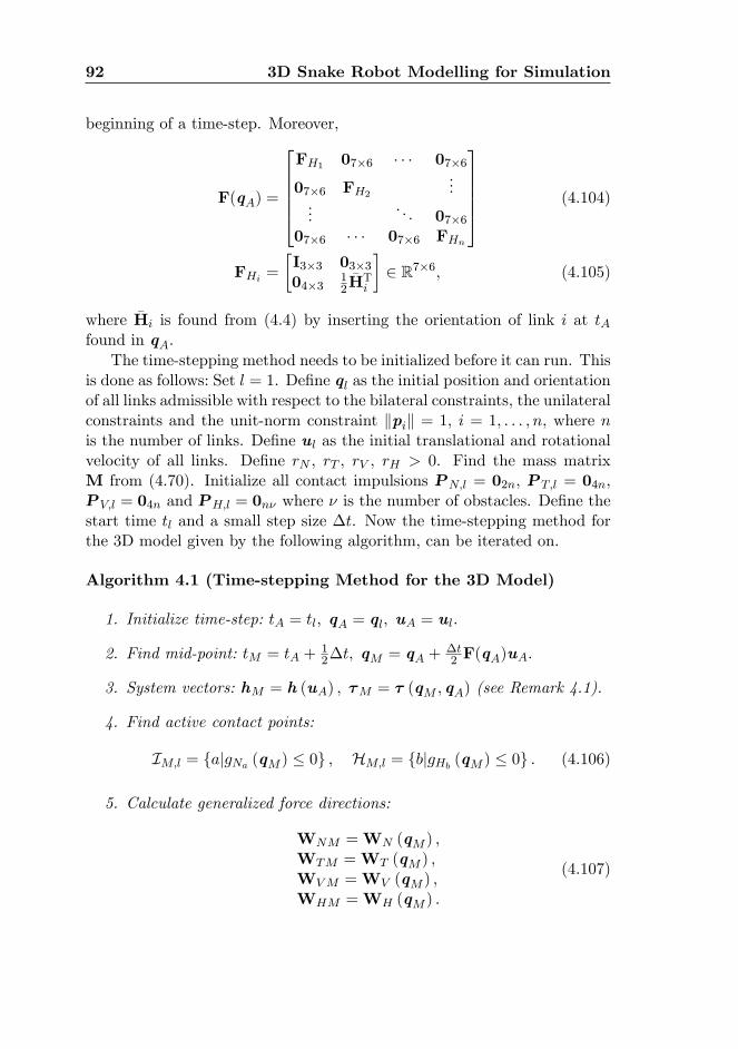
92 3D Snake Robot Modelling for Simulation
beginning of a time-step. Moreover,
F(qA) =
266664FH1 07�6 � � � 07�6
07�6 FH2...
.... . . 07�6
07�6 � � � 07�6 FHn
377775 (4.104)
FHi =
�I3�3 03�304�3
12�HTi
�2 R7�6; (4.105)
where �Hi is found from (4.4) by inserting the orientation of link i at tAfound in qA.
The time-stepping method needs to be initialized before it can run. Thisis done as follows: Set l = 1. De�ne ql as the initial position and orientationof all links admissible with respect to the bilateral constraints, the unilateralconstraints and the unit-norm constraint kpik = 1, i = 1; : : : ; n, where nis the number of links. De�ne ul as the initial translational and rotationalvelocity of all links. De�ne rN , rT , rV , rH > 0. Find the mass matrixM from (4.70). Initialize all contact impulsions PN;l = 02n, P T;l = 04n,P V;l = 04n and PH;l = 0n� where � is the number of obstacles. De�ne thestart time tl and a small step size �t. Now the time-stepping method forthe 3D model given by the following algorithm, can be iterated on.
Algorithm 4.1 (Time-stepping Method for the 3D Model)
1. Initialize time-step: tA = tl; qA = ql; uA = ul:
2. Find mid-point: tM = tA +12�t; qM = qA +
�t2 F(qA)uA:
3. System vectors: hM = h (uA) ; �M = � (qM ; qA) (see Remark 4.1).
4. Find active contact points:
IM;l = fajgNa (qM ) � 0g ; HM;l = fbjgHb (qM ) � 0g : (4.106)
5. Calculate generalized force directions:
WNM =WN (qM ) ;WTM =WT (qM ) ;WVM =WV (qM ) ;WHM =WH (qM ) :
(4.107)
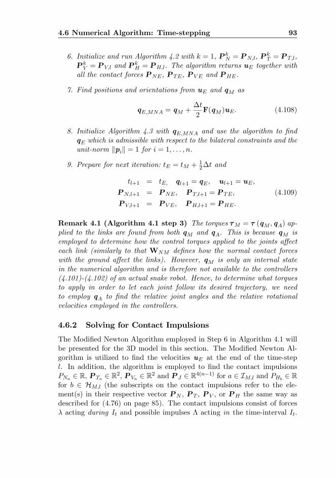
4.6 Numerical Algorithm: Time-stepping 93
6. Initialize and run Algorithm 4.2 with k = 1, P kN = PN;l, P k
T = P T;l,P kV = P V;l and P k
H = PH;l. The algorithm returns uE together withall the contact forces PNE, P TE, P V E and PHE.
7. Find positions and orientations from uE and qM as
qE;MNA = qM +�t
2F(qM )uE : (4.108)
8. Initialize Algorithm 4.3 with qE;MNA and use the algorithm to �ndqE which is admissible with respect to the bilateral constraints and theunit-norm kpik = 1 for i = 1; : : : ; n.
9. Prepare for next iteration: tE = tM + 12�t and
tl+1 = tE; ql+1 = qE ; ul+1 = uE ;
PN;l+1 = PNE ; P T;l+1 = P TE ; (4.109)
P V;l+1 = P V E ; PH;l+1 = PHE :
Remark 4.1 (Algorithm 4.1 step 3) The torques �M = � (qM ; qA) ap-plied to the links are found from both qM and qA. This is because qM isemployed to determine how the control torques applied to the joints a¤ecteach link (similarly to that WNM de�nes how the normal contact forceswith the ground a¤ect the links). However, qM is only an internal statein the numerical algorithm and is therefore not available to the controllers(4.101)-(4.102) of an actual snake robot. Hence, to determine what torquesto apply in order to let each joint follow its desired trajectory, we needto employ qA to �nd the relative joint angles and the relative rotationalvelocities employed in the controllers.
4.6.2 Solving for Contact Impulsions
The Modi�ed Newton Algorithm employed in Step 6 in Algorithm 4.1 willbe presented for the 3D model in this section. The Modi�ed Newton Al-gorithm is utilized to �nd the velocities uE at the end of the time-stepl. In addition, the algorithm is employed to �nd the contact impulsionsPNa 2 R, P Ta 2 R2, P Va 2 R2 and P J 2 R4(n�1) for a 2 IM;l and PHb 2 Rfor b 2 HM;l (the subscripts on the contact impulsions refer to the ele-ment(s) in their respective vector PN , P T , P V , or PH the same way asdescribed for (4.76) on page 85). The contact impulsions consist of forces� acting during It and possible impulses � acting in the time-interval It.
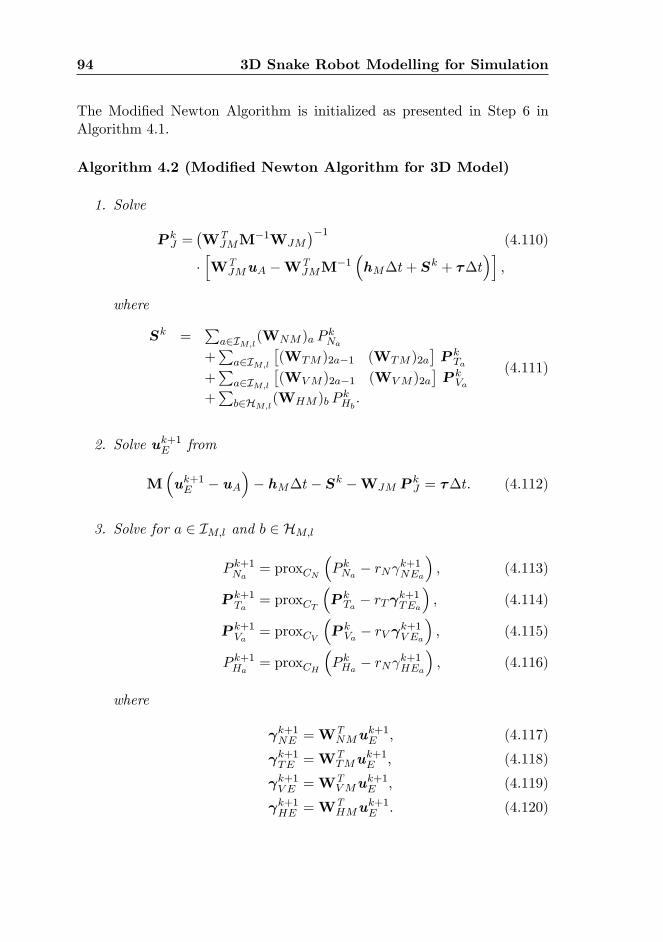
94 3D Snake Robot Modelling for Simulation
The Modi�ed Newton Algorithm is initialized as presented in Step 6 inAlgorithm 4.1.
Algorithm 4.2 (Modi�ed Newton Algorithm for 3D Model)
1. Solve
P kJ =
�WT
JMM�1WJM
��1(4.110)
�hWT
JMuA �WTJMM
�1�hM�t+ S
k + ��t�i;
where
Sk =P
a2IM;l(WNM )a P
kNa
+P
a2IM;l
�(WTM )2a�1 (WTM )2a
�P kTa
+P
a2IM;l
�(WVM )2a�1 (WVM )2a
�P kVa
+P
b2HM;l(WHM )b P
kHb:
(4.111)
2. Solve uk+1E from
M�uk+1E � uA
�� hM�t� Sk �WJM P
kJ = ��t: (4.112)
3. Solve for a 2 IM;l and b 2 HM;l
P k+1Na= proxCN
�P kNa � rN
k+1NEa
�; (4.113)
P k+1Ta
= proxCT
�P kTa � rT
k+1TEa
�; (4.114)
P k+1Va
= proxCV
�P kVa � rV
k+1V Ea
�; (4.115)
P k+1Ha= proxCH
�P kHa � rN
k+1HEa
�; (4.116)
where
k+1NE =WTNMu
k+1E ; (4.117)
k+1TE =WTTMu
k+1E ; (4.118)
k+1V E =WTVMu
k+1E ; (4.119)
k+1HE =WTHMu
k+1E : (4.120)
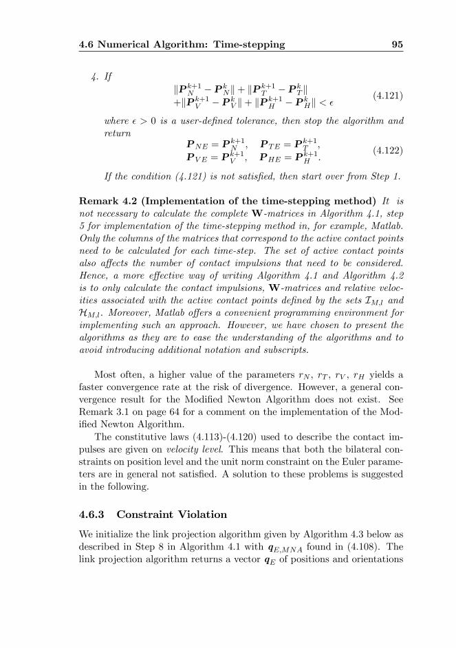
4.6 Numerical Algorithm: Time-stepping 95
4. IfkP k+1
N � P kNk+ kP k+1
T � P kT k
+kP k+1V � P k
V k+ kP k+1H � P k
Hk < �(4.121)
where � > 0 is a user-de�ned tolerance, then stop the algorithm andreturn
PNE = Pk+1N ; P TE = P
k+1T ;
P V E = Pk+1V ; PHE = P
k+1H :
(4.122)
If the condition (4.121) is not satis�ed, then start over from Step 1.
Remark 4.2 (Implementation of the time-stepping method) It isnot necessary to calculate the complete W-matrices in Algorithm 4.1, step5 for implementation of the time-stepping method in, for example, Matlab.Only the columns of the matrices that correspond to the active contact pointsneed to be calculated for each time-step. The set of active contact pointsalso a¤ects the number of contact impulsions that need to be considered.Hence, a more e¤ective way of writing Algorithm 4.1 and Algorithm 4.2is to only calculate the contact impulsions, W-matrices and relative veloc-ities associated with the active contact points de�ned by the sets IM;l andHM;l. Moreover, Matlab o¤ers a convenient programming environment forimplementing such an approach. However, we have chosen to present thealgorithms as they are to ease the understanding of the algorithms and toavoid introducing additional notation and subscripts.
Most often, a higher value of the parameters rN , rT , rV , rH yields afaster convergence rate at the risk of divergence. However, a general con-vergence result for the Modi�ed Newton Algorithm does not exist. SeeRemark 3.1 on page 64 for a comment on the implementation of the Mod-i�ed Newton Algorithm.
The constitutive laws (4.113)-(4.120) used to describe the contact im-pulses are given on velocity level. This means that both the bilateral con-straints on position level and the unit norm constraint on the Euler parame-ters are in general not satis�ed. A solution to these problems is suggestedin the following.
4.6.3 Constraint Violation
We initialize the link projection algorithm given by Algorithm 4.3 below asdescribed in Step 8 in Algorithm 4.1 with qE;MNA found in (4.108). Thelink projection algorithm returns a vector qE of positions and orientations
96 3D Snake Robot Modelling for Simulation
of the links which are admissible both to the bilateral constraints introducedby the joints and the unit-norm constraint on the quaternions.
Algorithm 4.3 (Projection of the Links)
1. Satisfy the unit-norm constraint kpik = 1 by setting
pEi =pE;MNAi
kpE;MNAik; i = 1; : : : ; n; (4.123)
where pE;MNAi is found from the vector qE;MNA and is the (non-unit-norm) quaternion. Let qE;quat be the new vector with positionsand the update orientations found with (4.123).
2. Employ qE;quat and let the orientation of link 1 be �xed. In addi-tion, let all the eBiz -axes be kept �xed. Now, change the e
Bix - and
eBiy -axis such that gJi� = 0 is satis�ed for i = 1; : : : ; n � 1, wherethe gap function gJi� is found in (4.20). This is achieved as followsfor i = 1; : : : ; n � 1: The current body axes can be found from thecorresponding rotation matrix as
RIBi
�qE;quat
�=�IeBix Ie
Biy Ie
Biz
�: (4.124)
Denote the new eBi+1x - and eBi+1y -axis eBi+1x and eBi+1y , respectively.Then we have that
eBi+1x =
eBiy � eBi+1z eBiy � eBi+1z
; (4.125)
eBi+1y =
eBi+1z � eBi+1x eBi+1z � eBi+1x
: (4.126)
Now, the new rotation matrix for link i+ 1 can be constructed as
RIBi+1 =
hI eBi+1x I e
Bi+1y Ie
Bi+1z
i; (4.127)
and the �nal quaternions describing the orientation of the link arefound from the new rotation matrix. Let qE;rot be the new coordinatevector with the updated quaternions.
3. Employ qE;rot and let the position of link 1 be �xed. Change thepositions of links i = 2; : : : ; n such that gJi� = 0 is satis�ed for i =1; : : : ; n�1, � = x; y; z where the gap function gJi� is given by (4.18).Let qE be the new coordinate vector with the updated positions. Now,return qE which satis�es the bilateral constraints and the unit-normconstraint.
4.7 Summary 97
4.7 Summary
We have extended the non-smooth (hybrid) 2D model presented in Chap-ter 3 to 3D motion. The model enables synthesis and testing of 3D snakerobot motion patterns. It is based on the framework of non-smooth dy-namics and convex analysis which allows us to easily and systematicallyincorporate unilateral contact forces (i.e. between the snake robot and theground surface and the obstacles) and friction forces based on Coulomb�slaw of dry friction. In addition, the particular choice of non-minimal coordi-nates results in an well arranged structure of the elements in the equality ofmeasures which describes the motion of the snake robot. Conventional nu-merical solvers can not be employed directly for numerical treatment of thenon-smooth model due to the set-valued force laws and possible instanta-neous velocity changes. Therefore, we show how to implement the model fornumerical treatment with the numerical integrator called the time-steppingmethod. This method helps to avoid explicit changes between equationsduring simulation even though the system is hybrid.

98 3D Snake Robot Modelling for Simulation
Chapter 5
Obstacle Aided Locomotion
5.1 Introduction
This chapter treats various aspects of obstacle aided locomotion with snakerobots in order to provide a better understanding of the simulation andexperimental results presented later in this thesis. We de�ne obstacle aidedlocomotion as snake robot locomotion where the snake robot utilizes wallsor other external objects, apart from the �at ground, for propulsion.
This chapter is based on Transeth et al. (2007b) and Transeth et al.(2008b) and it is organized as follows. We discuss the importance of obsta-cle aided locomotion in Section 5.2. In Section 5.3 a study by Gray (1946) isemployed to understand how snakes move forward by pushing against irreg-ularities in the ground. Requirements for obstacle aided locomotion for asnake robot are suggested in Section 5.4, while an approach to experimentalvalidation of obstacle aided locomotion is presented in Section 5.5.
5.2 Motivation
Biological snakes exploit objects and irregularities in their environmentto achieve more e¢ cient propulsion. A comparison with legged creaturesprovides an indication of this statement. While the gait displayed by alegged creature is highly dependent on the current speed of this creature,the gait displayed by a snake will mainly be dependent on the properties ofthe environment surrounding the snake. The �exibility and robust mobilityof snakes in cluttered environments is a signi�cant motivation for researchon snake robots. However, in order to fully bene�t from the advantages ofsnake locomotion in such environments, as illustrated in Figure 5.1, snake
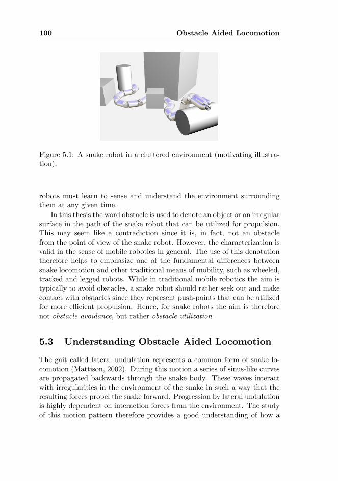
100 Obstacle Aided Locomotion
Figure 5.1: A snake robot in a cluttered environment (motivating illustra-tion).
robots must learn to sense and understand the environment surroundingthem at any given time.
In this thesis the word obstacle is used to denote an object or an irregularsurface in the path of the snake robot that can be utilized for propulsion.This may seem like a contradiction since it is, in fact, not an obstaclefrom the point of view of the snake robot. However, the characterization isvalid in the sense of mobile robotics in general. The use of this denotationtherefore helps to emphasize one of the fundamental di¤erences betweensnake locomotion and other traditional means of mobility, such as wheeled,tracked and legged robots. While in traditional mobile robotics the aim istypically to avoid obstacles, a snake robot should rather seek out and makecontact with obstacles since they represent push-points that can be utilizedfor more e¢ cient propulsion. Hence, for snake robots the aim is thereforenot obstacle avoidance, but rather obstacle utilization.
5.3 Understanding Obstacle Aided Locomotion
The gait called lateral undulation represents a common form of snake lo-comotion (Mattison, 2002). During this motion a series of sinus-like curvesare propagated backwards through the snake body. These waves interactwith irregularities in the environment of the snake in such a way that theresulting forces propel the snake forward. Progression by lateral undulationis highly dependent on interaction forces from the environment. The studyof this motion pattern therefore provides a good understanding of how a
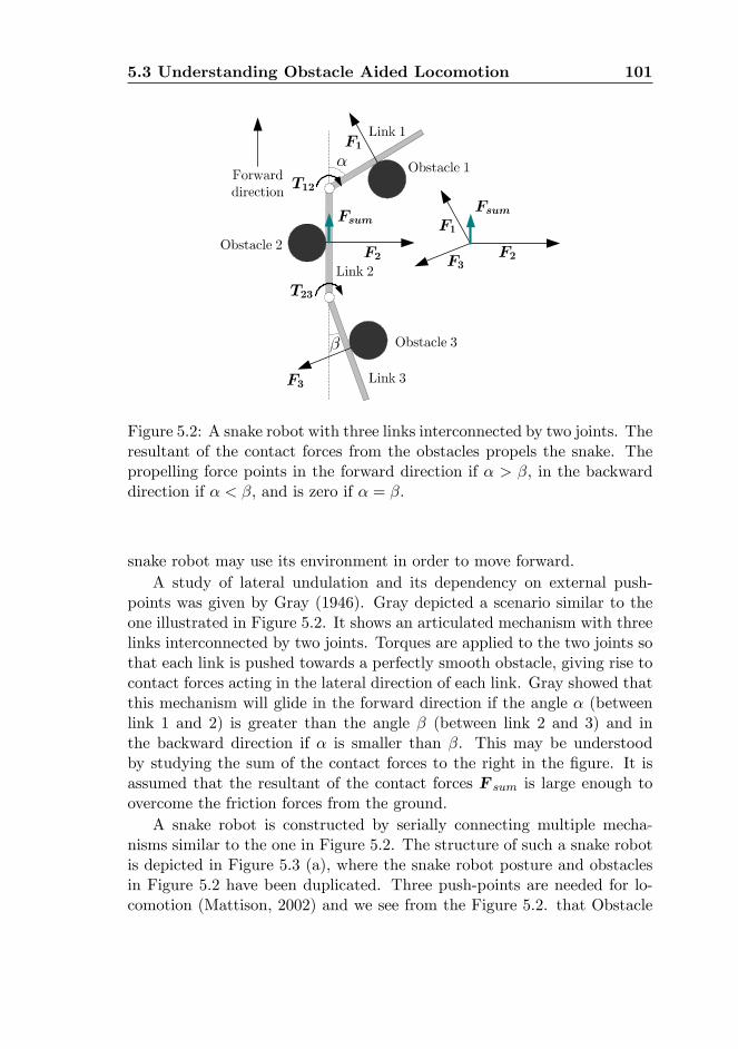
5.3 Understanding Obstacle Aided Locomotion 101
Figure 5.2: A snake robot with three links interconnected by two joints. Theresultant of the contact forces from the obstacles propels the snake. Thepropelling force points in the forward direction if � > �, in the backwarddirection if � < �, and is zero if � = �.
snake robot may use its environment in order to move forward.A study of lateral undulation and its dependency on external push-
points was given by Gray (1946). Gray depicted a scenario similar to theone illustrated in Figure 5.2. It shows an articulated mechanism with threelinks interconnected by two joints. Torques are applied to the two joints sothat each link is pushed towards a perfectly smooth obstacle, giving rise tocontact forces acting in the lateral direction of each link. Gray showed thatthis mechanism will glide in the forward direction if the angle � (betweenlink 1 and 2) is greater than the angle � (between link 2 and 3) and inthe backward direction if � is smaller than �. This may be understoodby studying the sum of the contact forces to the right in the �gure. It isassumed that the resultant of the contact forces F sum is large enough toovercome the friction forces from the ground.
A snake robot is constructed by serially connecting multiple mecha-nisms similar to the one in Figure 5.2. The structure of such a snake robotis depicted in Figure 5.3 (a), where the snake robot posture and obstaclesin Figure 5.2 have been duplicated. Three push-points are needed for lo-comotion (Mattison, 2002) and we see from the Figure 5.2. that Obstacle
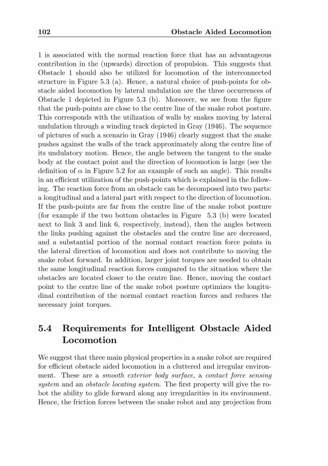
102 Obstacle Aided Locomotion
1 is associated with the normal reaction force that has an advantageouscontribution in the (upwards) direction of propulsion. This suggests thatObstacle 1 should also be utilized for locomotion of the interconnectedstructure in Figure 5.3 (a). Hence, a natural choice of push-points for ob-stacle aided locomotion by lateral undulation are the three occurrences ofObstacle 1 depicted in Figure 5.3 (b). Moreover, we see from the �gurethat the push-points are close to the centre line of the snake robot posture.This corresponds with the utilization of walls by snakes moving by lateralundulation through a winding track depicted in Gray (1946). The sequenceof pictures of such a scenario in Gray (1946) clearly suggest that the snakepushes against the walls of the track approximately along the centre line ofits undulatory motion. Hence, the angle between the tangent to the snakebody at the contact point and the direction of locomotion is large (see thede�nition of � in Figure 5.2 for an example of such an angle). This resultsin an e¢ cient utilization of the push-points which is explained in the follow-ing. The reaction force from an obstacle can be decomposed into two parts:a longitudinal and a lateral part with respect to the direction of locomotion.If the push-points are far from the centre line of the snake robot posture(for example if the two bottom obstacles in Figure 5.3 (b) were locatednext to link 3 and link 6, respectively, instead), then the angles betweenthe links pushing against the obstacles and the centre line are decreased,and a substantial portion of the normal contact reaction force points inthe lateral direction of locomotion and does not contribute to moving thesnake robot forward. In addition, larger joint torques are needed to obtainthe same longitudinal reaction forces compared to the situation where theobstacles are located closer to the centre line. Hence, moving the contactpoint to the centre line of the snake robot posture optimizes the longitu-dinal contribution of the normal contact reaction forces and reduces thenecessary joint torques.
5.4 Requirements for Intelligent Obstacle AidedLocomotion
We suggest that three main physical properties in a snake robot are requiredfor e¢ cient obstacle aided locomotion in a cluttered and irregular environ-ment. These are a smooth exterior body surface, a contact force sensingsystem and an obstacle locating system. The �rst property will give the ro-bot the ability to glide forward along any irregularities in its environment.Hence, the friction forces between the snake robot and any projection from
5.4 Requirements for Intelligent Obstacle Aided Locomotion 103
Figure 5.3: Snake robot (a) with all obstacles from Figure 5.2, and (b) withonly the necessary and most suited obstacles for locomotion.
104 Obstacle Aided Locomotion
the ground used as a push-point should be as low as possible. Moreover,it will mimic the skin of a biological snake more closely. Any irregularitieson the body surface of the snake robot will potentially obstruct the glidingmotion of the robot. The second property is crucial for intelligent obstacleutilization. Contact force sensing allows the snake robot to detect when thebody is in contact with a push-point and also control the force exerted ona push-point. Since the sum of contact forces along the snake body is whatpropels the robot forward, the ability to measure these forces is importantin order to be able to control the propulsion. The third property enablesthe snake robot to search for new push-points which it is not currently ableto touch (i.e. sense with the force sensors).
A control strategy for obstacle aided locomotion should in general con-sist of two continuous tasks running in parallel. The function of the �rsttask should be high-level motion planning. This task should establish somesort of map of the environment surrounding the snake robot and use it toplan a path through this environment. In contrast to conventional pathplanning strategies for mobile robots, the goal should not be to avoid ob-stacles, but rather to move relative to these irregularities in a way thatenables the snake robot to utilize push-points for more e¢ cient propulsion.
The actual obstacle utilization should be continuously carried out in thesecond task as a function of the current force measurements along the bodyand the desired direction of motion. This task should basically control thejoints of the snake robot so that the sum of the contact forces along thesnake body is pointing toward the desired direction of motion.
One of the purposes of this thesis is to present a mathematical frame-work for the study of obstacle aided locomotion. This thesis will thereforenot treat the speci�c implementation of the motion controller discussedabove. However, we note that all the three above main physical propertiesare in e¤ect available in the mathematical model presented in this thesis:The exterior of the snake robot model is smooth, we are able to calcu-late the forces between the snake robot and the obstacles and we have anobstacle locating system since the position of all obstacles are known in ad-vance. Hence, the model can be employed to test intelligent obstacle aidedlocomotion when such future control schemes are developed.
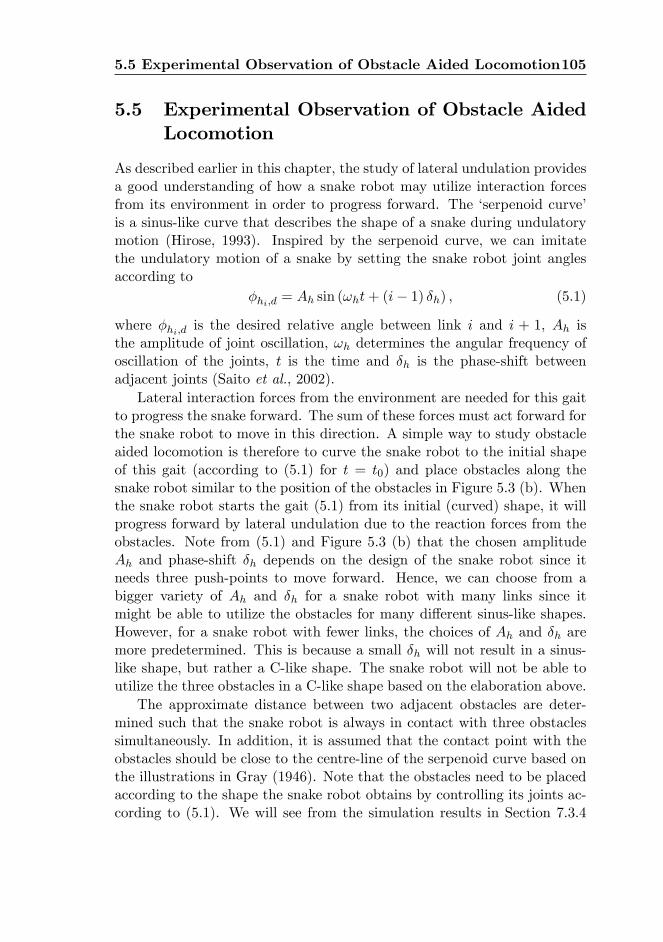
5.5 Experimental Observation of Obstacle Aided Locomotion105
5.5 Experimental Observation of Obstacle AidedLocomotion
As described earlier in this chapter, the study of lateral undulation providesa good understanding of how a snake robot may utilize interaction forcesfrom its environment in order to progress forward. The �serpenoid curve�is a sinus-like curve that describes the shape of a snake during undulatorymotion (Hirose, 1993). Inspired by the serpenoid curve, we can imitatethe undulatory motion of a snake by setting the snake robot joint anglesaccording to
�hi;d = Ah sin (!ht+ (i� 1) �h) ; (5.1)
where �hi;d is the desired relative angle between link i and i + 1, Ah isthe amplitude of joint oscillation, !h determines the angular frequency ofoscillation of the joints, t is the time and �h is the phase-shift betweenadjacent joints (Saito et al., 2002).
Lateral interaction forces from the environment are needed for this gaitto progress the snake forward. The sum of these forces must act forward forthe snake robot to move in this direction. A simple way to study obstacleaided locomotion is therefore to curve the snake robot to the initial shapeof this gait (according to (5.1) for t = t0) and place obstacles along thesnake robot similar to the position of the obstacles in Figure 5.3 (b). Whenthe snake robot starts the gait (5.1) from its initial (curved) shape, it willprogress forward by lateral undulation due to the reaction forces from theobstacles. Note from (5.1) and Figure 5.3 (b) that the chosen amplitudeAh and phase-shift �h depends on the design of the snake robot since itneeds three push-points to move forward. Hence, we can choose from abigger variety of Ah and �h for a snake robot with many links since itmight be able to utilize the obstacles for many di¤erent sinus-like shapes.However, for a snake robot with fewer links, the choices of Ah and �h aremore predetermined. This is because a small �h will not result in a sinus-like shape, but rather a C-like shape. The snake robot will not be able toutilize the three obstacles in a C-like shape based on the elaboration above.
The approximate distance between two adjacent obstacles are deter-mined such that the snake robot is always in contact with three obstaclessimultaneously. In addition, it is assumed that the contact point with theobstacles should be close to the centre-line of the serpenoid curve based onthe illustrations in Gray (1946). Note that the obstacles need to be placedaccording to the shape the snake robot obtains by controlling its joints ac-cording to (5.1). We will see from the simulation results in Section 7.3.4
106 Obstacle Aided Locomotion
that a slight variation of the position of one obstacle does not seriouslya¤ect ability of the snake robot to move forward. However, if an obstacle ismoved far away from its original position, then the snake robot is not ableto complete its track while following the preprogrammed motion patterngiven by (5.1). The snake robot needs to be equipped with sensors to detectcontact with the obstacles for a scenario with randomly placed obstaclesand this is beyond the scope of this thesis.
A real rescue operation in a shattered building will require a snake robotwith a smooth and sealed exterior. This avoids that small pieces of rubbleget stuck in the joints of the snake robot and hinders it to move. However,the principle motion pattern for how to move in such an environment canbe studied in a laboratory setting without having developed a robust snakerobot design �rst. To this end, we simply choose the obstacles large enoughso that they do not get stuck in the snake robot joints. This is advantageoussince it reduces the development time and cost of the snake robot used inthe experiments. Moreover, the basics of obstacle aided locomotion arethe same for small and large obstacles since the fundamental goal is stillto allocate enough push-points such that the snake robot is able to moveforward.
Chapter 6
Modelling and Control of aPlanar Snake Robot
6.1 Introduction
Many authors base the choice and implementation of the most commonserpentine motion pattern called lateral undulation on the serpenoid curvefound in Hirose (1993). This is a curve that describes the motion of a bi-ological snake while moving by lateral undulation, and a snake robot canfollow an approximation to this curve by setting its joint angles accordingto a sine-curve that is phase-shifted between adjacent joints. This approachto snake robot locomotion has been widely implemented for snake robotsthat have either wheels (Ostrowski and Burdick, 1996; Prautsch and Mita,1999) or a friction property such that each link of the snake robot glideseasier forward and backward compared to transversal motion (Ma, 2001;Saito et al., 2002). A no-slip constraint (i.e. a non-holonomic velocity con-straint) on each wheel is sometimes introduced in the mathematical model,thus avoiding that a link slips sideways. Such an approach is presentedin Prautsch and Mita (1999), where the no-slip constraint allows one tosigni�cantly reduce the model. A Lyapunov-based proof for this reducedmodel together with a proposed controller shows that the snake robot isable to move to a position reference. A controller for the velocity and head-ing for a wheel-less snake robot with the friction property described above,is presented in Saito et al. (2002). The simulation and experimental resultspresented in that paper indicate that the snake robot is able to stay within areasonable o¤set of the desired speed. However, no formal stability analysisof the closed-loop system is given. For wheel-less snake robots it is not al-
108 Modelling and Control of a Planar Snake Robot
ways su¢ cient to consider a purely kinematic model for the motion patternlateral undulation, as the friction between the snake robot and the groundsurface may be essential for locomotion. Therefore, the friction needs tobe considered for wheel-less snake robots and this motivates including thedynamics into controller synthesis and stability analysis of the snake robot.
The above published results all consider control of the position or orien-tation of a selection of snake robot links or some mean value of the velocityand orientation of all the links of a snake robot. Hence, the main concernis where some point on the snake robot is in space or where it is headingwith what velocity. However, for delicate operations such as inspection andmaintenance in industrial plants, every point on the snake robot body needto be accurately controlled. As a �rst step toward designing such a controlscheme, we present in this chapter an input-output linearizing controllerfor tracking control of snake robot joints. Such model-based control of theinternal con�guration of the snake robot has, to the best of our knowledge,not been investigated before, and it results in a challenging stability analysisdue to the large number of degrees of freedom that needs to be considered.It is hoped that the results presented in this chapter can be combined withthe controllers presented for control of the position and/or orientation ofthe snake robot to be able to accurately control both the global position ofthe snake robot in the plane together with precise control of the internalcon�guration of the snake robot. This way, every point on the snake robotbody relative to some �xed point in space can be accurately controlled.
In the previous chapters on modelling of a snake robot, we focusedon developing mathematical models for realistic and e¢ cient simulationsof planar and 3D snake robot motion. In this chapter we shift the mainfocus to control. To this end, we develop a new 2D model of the snakerobot based on the standard robot manipulator model commonly employedto model robot manipulators (usually with less degrees of freedom thana snake robot) and marine vessels (Fossen, 2002; Spong and Vidyasagar,1989). This model is denoted as the process plant model. By employing thisparticular form of the model, a large area of techniques regarding controland stability analysis of such systems becomes available. However, thisrepresentation of a model of a snake robot (with such a large number ofdegrees of freedom) is not advantageous for simulation as will be shownin Section 7.3.5 so the 2D model developed earlier in this chapter is stillimportant. The process plant model contains the global orientation of thesnake robot. However, to make the stability analysis manageable we derivea control plant model from the process plant model where this orientation is
6.2 Mathematical Modelling 109
removed. In this chapter, we employ one group of the techniques availablefor the robot manipulator model, called input-output linearization (Khalil,2002; Nijmeijer and Schaft, 1990) to develop a controller for tracking controlof the snake robot joints, and we show, using the control plant model, thatthe joint angles converge exponentially to their desired trajectory. Thenon-linear control techniques employed in this chapter are generally only �tto cope with smooth non-linear systems. Moreover, few control techniquesexists for non-smooth systems such as the 2D model presented in Chapter 3.Therefore, in order to make the control problem tractable, we approximatethe Coulomb friction with a smooth friction model and design a non-linearcontrol law for the resulting smooth system. Note that we do not give areference for the global position and orientation of the snake robot whichis beyond the scope of this thesis. Instead, we focus on proving that eachjoint is able to track a desired reference angle.
This chapter is based on Transeth et al. (2007a) and it is organizedas follows. Section 6.2 presents mathematical models, both based on thestandard dynamics of a robot manipulator, of the snake robot and usedfor simulation and stability analysis, respectively. The controller and thestability analysis are given in Section 6.3 and a summary of the chapter isfound in Section 6.4.
6.2 Mathematical Modelling
In this section we �rst develop the mathematical model of a planar snakerobot without wheels based on the standard model for a robot manipula-tor with minimal coordinates found in for example Spong and Vidyasagar(1989). We denote this model the process plant model and implement itfor two di¤erent constitutive laws for Coulomb friction. The process plantmodel is necessary for us to be able to proceed to the next step which is toreformulate the process plant model to obtain a control plant model usedboth for designing the joint controllers and for deriving stability resultsfor the closed-loop system. The process plant model di¤ers mainly fromthe 2D model presented in Chapter 3 in that the model is described by anordinary di¤erential equation (ODE) instead of an equality of measures, asmooth approximation to the Coulomb friction is employed, and minimalcoordinates are used to describe the kinematics.
The snake robot di¤ers from a regular robot manipulator in that ex-ternal forces act on each link instead of just the end-e¤ector. This callsfor a more extensive use of the various manipulator Jacobians employed
110 Modelling and Control of a Planar Snake Robot
to �nd the velocities of each link from the time-derivative of the minimalcoordinates and also to include the friction forces in the system dynamics.
Before we proceed with the modelling, let us �rst sum up the variousplanar models we have discussed so far. The �2D model� is presented inChapter 3 and is developed for e¢ cient simulations. In this section, wealso develop a 2D model denoted the �process plant model�, and this modelcan also be employed for simulation. However, it is not advantageous forsimulation partly due to the large number of degrees of freedom of a snakerobot which results in large system matrices. Nonetheless, it may be conve-nient to employ the process plant model for simulation just in order to testthe controller since many of the system matrices utilized in the controllerare already available in the numerical treatment of the model. From theprocess plant model, we will develop a �control plant model�for designingthe model-based controller and for stability analysis. We will sometimesrefer to the process plant model as the �robot model�throughout this thesisin order to distinguish it from the �2D model�from Chapter 3.
6.2.1 Process Plant Model
In this section we derive a mathematical model of a wheel-less snake robotbased on the Euler-Lagrange equations as found in, for example, Spongand Vidyasagar (1989). This model is denoted the process plant model.We present two models for the Coulomb friction between the snake robotand the ground. The �rst model is a smooth approximation to the Coulombfriction. This approximation is performed to be able to employ standardtechniques for controller design. The second friction model is a model of set-valued Coulomb friction using a set-valued force law (similar to Chapter 3).We implement the latter model to check how the controller works for a morerealistic model of a snake robot.
In the following we will �rst describe the kinematics and then we presentthe dynamics of the snake robot.
Kinematics and Velocities
The 2D snake robot model presented in this chapter consists of n� 2 equallinks connected by n � 3 revolute joints, each with one degree of freedom(DOF). See Figure 6.1 for an illustration of a snake robot with four links.The inertial position and orientation of the snake robot adds three DOFto the model. As opposed to n being the number of links in the previouschapters, notice that n now describes the number of DOF of the system. To
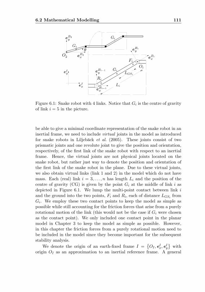
6.2 Mathematical Modelling 111
Figure 6.1: Snake robot with 4 links. Notice that Gi is the centre of gravityof link i = 5 in the picture.
be able to give a minimal coordinate representation of the snake robot in aninertial frame, we need to include virtual joints in the model as introducedfor snake robots in Liljebäck et al. (2005). These joints consist of twoprismatic joints and one revolute joint to give the position and orientation,respectively, of the �rst link of the snake robot with respect to an inertialframe. Hence, the virtual joints are not physical joints located on thesnake robot, but rather just way to denote the position and orientation ofthe �rst link of the snake robot in the plane. Due to these virtual joints,we also obtain virtual links (link 1 and 2) in the model which do not havemass. Each (real) link i = 3; : : : ; n has length Li and the position of thecentre of gravity (CG) is given by the point Gi at the middle of link i asdepicted in Figure 6.1. We lump the multi-point contact between link iand the ground into the two points, Fi and Ri, each of distance LGSi fromGi. We employ these two contact points to keep the model as simple aspossible while still accounting for the friction forces that arise from a purelyrotational motion of the link (this would not be the case if Gi were chosenas the contact point). We only included one contact point in the planarmodel in Chapter 3 to keep the model as simple as possible. However,in this chapter the friction forces from a purely rotational motion need tobe included in the model since they become important for the subsequentstability analysis.
We denote the origin of an earth-�xed frame I =�OI ; e
Ix; e
Iy
with
origin OI as an approximation to an inertial reference frame. A general
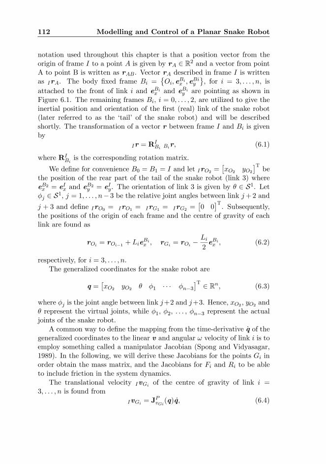
112 Modelling and Control of a Planar Snake Robot
notation used throughout this chapter is that a position vector from theorigin of frame I to a point A is given by rA 2 R2 and a vector from pointA to point B is written as rAB. Vector rA described in frame I is writtenas IrA. The body �xed frame Bi =
�Oi; e
Bix ; e
Biy
, for i = 3; : : : ; n, is
attached to the front of link i and eBix and eBiy are pointing as shown inFigure 6.1. The remaining frames Bi, i = 0; : : : ; 2, are utilized to give theinertial position and orientation of the �rst (real) link of the snake robot(later referred to as the �tail� of the snake robot) and will be describedshortly. The transformation of a vector r between frame I and Bi is givenby
Ir = RIBi Bir; (6.1)
where RIBiis the corresponding rotation matrix.
We de�ne for convenience B0 = B1 = I and let IrO2 =�xO2 yO2
�Tbe
the position of the rear part of the tail of the snake robot (link 3) whereeB2x = eIx and e
B2y = eIy. The orientation of link 3 is given by � 2 S1. Let
�j 2 S1, j = 1; : : : ; n� 3 be the relative joint angles between link j+2 andj + 3 and de�ne IrO0 = IrO1 = IrG1 = IrG2 =
�0 0
�T. Subsequently,
the positions of the origin of each frame and the centre of gravity of eachlink are found as
rOi = rOi�1 + LieBix ; rGi = rOi �
Li2eBix ; (6.2)
respectively, for i = 3; : : : ; n.The generalized coordinates for the snake robot are
q =�xO2 yO2 � �1 � � � �n�3
�T 2 Rn; (6.3)
where �j is the joint angle between link j+2 and j+3. Hence, xO2 , yO2 and� represent the virtual joints, while �1, �2, . . . , �n�3 represent the actualjoints of the snake robot.
A common way to de�ne the mapping from the time-derivative _q of thegeneralized coordinates to the linear v and angular ! velocity of link i is toemploy something called a manipulator Jacobian (Spong and Vidyasagar,1989). In the following, we will derive these Jacobians for the points Gi inorder obtain the mass matrix, and the Jacobians for Fi and Ri to be ableto include friction in the system dynamics.
The translational velocity IvGi of the centre of gravity of link i =3; : : : ; n is found from
IvGi = JPvGi(q) _q; (6.4)
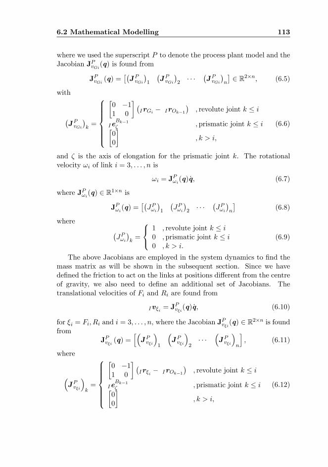
6.2 Mathematical Modelling 113
where we used the superscript P to denote the process plant model and theJacobian JPvGi(q) is found from
JPvGi (q) =��JPvGi
�1
�JPvGi
�2� � �
�JPvGi
�n
�2 R2�n; (6.5)
with
�JPvGi
�k=
8>>>>><>>>>>:
�0 �11 0
� �IrGi � IrOk�1
�; revolute joint k � i
IeBk�1� ;prismatic joint k � i�00
�; k > i;
(6.6)
and � is the axis of elongation for the prismatic joint k. The rotationalvelocity !i of link i = 3; : : : ; n is
!i = JP!i(q) _q; (6.7)
where JP!i(q) 2 R1�n is
JP!i(q) =��JP!i�1
�JP!i�2� � �
�JP!i�n
�(6.8)
where �JP!i�k=
8<:1 ; revolute joint k � i0 ;prismatic joint k � i0 ; k > i:
(6.9)
The above Jacobians are employed in the system dynamics to �nd themass matrix as will be shown in the subsequent section. Since we havede�ned the friction to act on the links at positions di¤erent from the centreof gravity, we also need to de�ne an additional set of Jacobians. Thetranslational velocities of Fi and Ri are found from
Iv�i = JPv�i(q) _q; (6.10)
for �i = Fi; Ri and i = 3; : : : ; n, where the Jacobian JPv�i(q) 2 R2�n is found
fromJPv�i (q) =
h�JPv�i
�1
�JPv�i
�2� � �
�JPv�i
�n
i; (6.11)
where
�JPv�i
�k=
8>>>>><>>>>>:
�0 �11 0
� �Ir�i � IrOk�1
�; revolute joint k � i
IeBk�1� ;prismatic joint k � i�00
�; k > i;
(6.12)
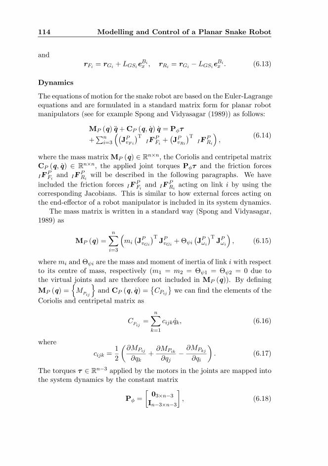
114 Modelling and Control of a Planar Snake Robot
andrFi = rGi + LGSie
Bix ; rRi = rGi � LGSieBix : (6.13)
Dynamics
The equations of motion for the snake robot are based on the Euler-Lagrangeequations and are formulated in a standard matrix form for planar robotmanipulators (see for example Spong and Vidyasagar (1989)) as follows:
MP (q) �q +CP (q; _q) _q = P��
+Pn
i=3
��JPvFi
�TIF
PFi+�JPvRi
�TIF
PRi
�;
(6.14)
where the mass matrixMP (q) 2 Rn�n, the Coriolis and centripetal matrixCP (q; _q) 2 Rn�n, the applied joint torques P�� and the friction forcesIF
PFiand IF
PRiwill be described in the following paragraphs. We have
included the friction forces IF PFiand IF
PRiacting on link i by using the
corresponding Jacobians. This is similar to how external forces acting onthe end-e¤ector of a robot manipulator is included in its system dynamics.
The mass matrix is written in a standard way (Spong and Vidyasagar,1989) as
MP (q) =nXi=3
�mi
�JPvGi
�TJPvGi +� i
�JP!i�TJP!i
�; (6.15)
where mi and � i are the mass and moment of inertia of link i with respectto its centre of mass, respectively (m1 = m2 = � 1 = � 2 = 0 due tothe virtual joints and are therefore not included in MP (q)). By de�ning
MP (q) =nMPij
oand CP (q; _q) =
�CPij
we can �nd the elements of the
Coriolis and centripetal matrix as
CPij=
nXk=1
cijk _qk; (6.16)
where
cijk =1
2
�@MPij
@qk+@MPik
@qj�@MPkj
@qi
�: (6.17)
The torques � 2 Rn�3 applied by the motors in the joints are mapped intothe system dynamics by the constant matrix
P� =
�03�n�3In�3�n�3
�; (6.18)
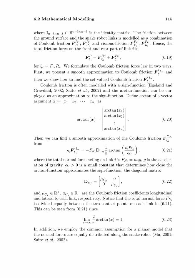
6.2 Mathematical Modelling 115
where In�3�n�3 2 Rn�3�n�3 is the identity matrix. The friction betweenthe ground surface and the snake robot links is modelled as a combinationof Coulomb friction F PC
Fi, F PC
Riand viscous friction F PV
Fi, F PV
Ri. Hence, the
total friction force on the front and rear part of link i is
F P�i= F PC
�i+ F PV
�i; (6.19)
for �i = Fi; Ri. We formulate the Coulomb friction force law in two ways.First, we present a smooth approximation to Coulomb friction F PCc
�iand
then we show how to �nd the set-valued Coulomb friction FPCt�i.
Coulomb friction is often modelled with a sign-function (Egeland andGravdahl, 2002; Saito et al., 2002) and the arctan-function can be em-ployed as an approximation to the sign-function. De�ne arctan of a vectorargument x =
�x1 x2 � � � xn
�as
arctan (x) =
26664arctan (x1)arctan (x2)
...arctan (xn)
37775 : (6.20)
Then we can �nd a smooth approximation of the Coulomb friction F PCc�i
from
BiFPCc�i
= �FNiD�C
1
�arctan
�Biv�i�C
�; (6.21)
where the total normal force acting on link i is FNi = mig, g is the acceler-ation of gravity, �C > 0 is a small constant that determines how close thearctan-function approximates the sign-function, the diagonal matrix
D�C =
��Cx 00 �Cy
�; (6.22)
and �Cx 2 R+, �Cy 2 R+ are the Coulomb friction coe¢ cients longitudinaland lateral to each link, respectively. Notice that the total normal force FNiis divided equally between the two contact points on each link in (6.21).This can be seen from (6.21) since
limx!1
2
�arctan (x) = 1: (6.23)
In addition, we employ the common assumption for a planar model thatthe normal forces are equally distributed along the snake robot (Ma, 2001;Saito et al., 2002).
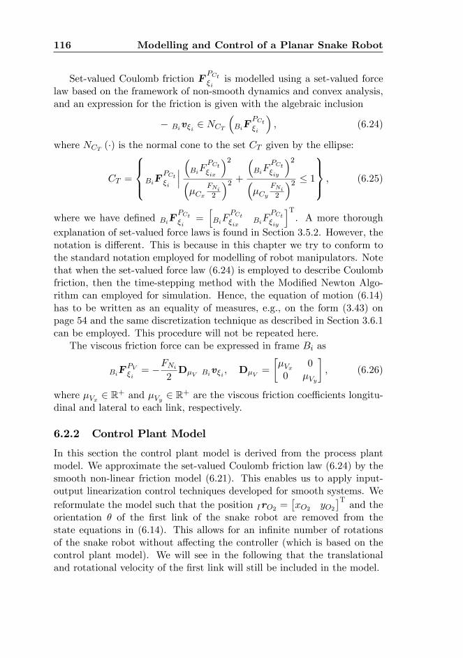
116 Modelling and Control of a Planar Snake Robot
Set-valued Coulomb friction FPCt�i
is modelled using a set-valued forcelaw based on the framework of non-smooth dynamics and convex analysis,and an expression for the friction is given with the algebraic inclusion
� Biv�i 2 NCT
�BiF
PCt�i
�; (6.24)
where NCT (�) is the normal cone to the set CT given by the ellipse:
CT =
8><>:BiFPCt�i
����BiF
PCt�ix
�2��Cx
FNi2
�2 +�BiF
PCt�iy
�2��Cy
FNi2
�2 � 19>=>; ; (6.25)
where we have de�ned BiFPCt�i
=hBiF
PCt�ix BiF
PCt�iy
iT. A more thorough
explanation of set-valued force laws is found in Section 3.5.2. However, thenotation is di¤erent. This is because in this chapter we try to conform tothe standard notation employed for modelling of robot manipulators. Notethat when the set-valued force law (6.24) is employed to describe Coulombfriction, then the time-stepping method with the Modi�ed Newton Algo-rithm can employed for simulation. Hence, the equation of motion (6.14)has to be written as an equality of measures, e.g., on the form (3.43) onpage 54 and the same discretization technique as described in Section 3.6.1can be employed. This procedure will not be repeated here.
The viscous friction force can be expressed in frame Bi as
BiFPV�i= �FNi
2D�V Biv�i ; D�V =
��Vx 00 �Vy
�; (6.26)
where �Vx 2 R+ and �Vy 2 R+ are the viscous friction coe¢ cients longitu-dinal and lateral to each link, respectively.
6.2.2 Control Plant Model
In this section the control plant model is derived from the process plantmodel. We approximate the set-valued Coulomb friction law (6.24) by thesmooth non-linear friction model (6.21). This enables us to apply input-output linearization control techniques developed for smooth systems. Wereformulate the model such that the position IrO2 =
�xO2 yO2
�Tand the
orientation � of the �rst link of the snake robot are removed from thestate equations in (6.14). This allows for an in�nite number of rotationsof the snake robot without a¤ecting the controller (which is based on thecontrol plant model). We will see in the following that the translationaland rotational velocity of the �rst link will still be included in the model.
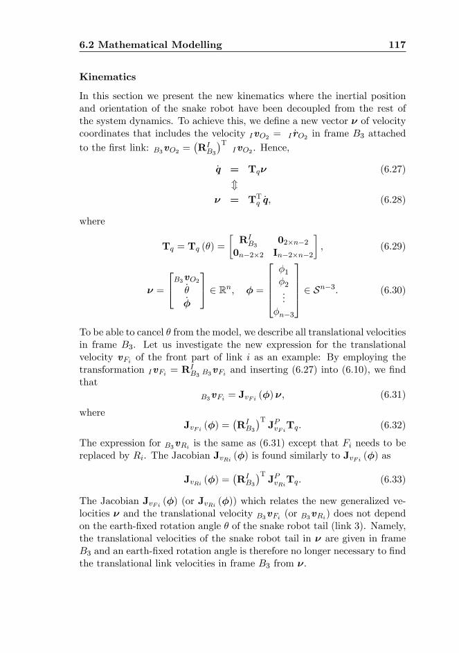
6.2 Mathematical Modelling 117
Kinematics
In this section we present the new kinematics where the inertial positionand orientation of the snake robot have been decoupled from the rest ofthe system dynamics. To achieve this, we de�ne a new vector � of velocitycoordinates that includes the velocity IvO2 = I _rO2 in frame B3 attachedto the �rst link: B3vO2 =
�RIB3
�TIvO2 . Hence,
_q = Tq� (6.27)
m� = TTq _q; (6.28)
where
Tq = Tq (�) =
�RIB3
02�n�20n�2�2 In�2�n�2
�; (6.29)
� =
24B3vO2_�_�
35 2 Rn; � =
26664�1�2...
�n�3
37775 2 Sn�3: (6.30)
To be able to cancel � from the model, we describe all translational velocitiesin frame B3. Let us investigate the new expression for the translationalvelocity vFi of the front part of link i as an example: By employing thetransformation IvFi = R
IB3 B3
vFi and inserting (6.27) into (6.10), we �ndthat
B3vFi = JvFi (�)�; (6.31)
whereJvFi (�) =
�RIB3
�TJPvFiTq: (6.32)
The expression for B3vRi is the same as (6.31) except that Fi needs to bereplaced by Ri. The Jacobian JvRi (�) is found similarly to JvFi (�) as
JvRi (�) =�RIB3
�TJPvRiTq: (6.33)
The Jacobian JvFi (�) (or JvRi (�)) which relates the new generalized ve-locities � and the translational velocity B3vFi (or B3vRi) does not dependon the earth-�xed rotation angle � of the snake robot tail (link 3). Namely,the translational velocities of the snake robot tail in � are given in frameB3 and an earth-�xed rotation angle is therefore no longer necessary to �ndthe translational link velocities in frame B3 from �.
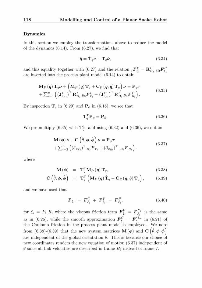
118 Modelling and Control of a Planar Snake Robot
Dynamics
In this section we employ the transformations above to reduce the modelof the dynamics (6.14). From (6.27), we �nd that
�q = _Tq� +Tq _�; (6.34)
and this equality together with (6.27) and the relation IFP�i= RI
B3 B3FP�i
are inserted into the process plant model (6.14) to obtain
MP (q)Tq _� +�MP (q) _Tq +CP (q; _q)Tq
�� = P��
+Pn
i=3
��JPvFi
�TRIB3 B3
F PFi+�JPvRi
�TRIB3 B3
F PRi
�:
(6.35)
By inspection Tq in (6.29) and P� in (6.18), we see that
TTq P� = P�: (6.36)
We pre-multiply (6.35) with TTq , and using (6.32) and (6.36), we obtain
M (�) _� +C�_�;�; _�
�� = P��
+Pn
i=3
�(JvFi)
TB3F Fi + (JvRi)
TB3FRi
�:
(6.37)
where
M (�) = TTqMP (q)Tq; (6.38)
C�_�;�; _�
�= TTq
�MP (q) _Tq +CP (q; _q)Tq
�; (6.39)
and we have used that
F �i = FC�i+ F V
�i= F P
�i; (6.40)
for �i = Fi; Ri where the viscous friction term F V�i= F PV
�iis the same
as in (6.26), while the smooth approximation FC�i= F
PCc�i
in (6.21) ofthe Coulomb friction in the process plant model is employed. We note
from (6.38)-(6.39) that the new system matrices M (�) and C�_�;�; _�
�are independent of the global orientation �. This is because our choice ofnew coordinates renders the new equation of motion (6.37) independent of� since all link velocities are described in frame B3 instead of frame I.
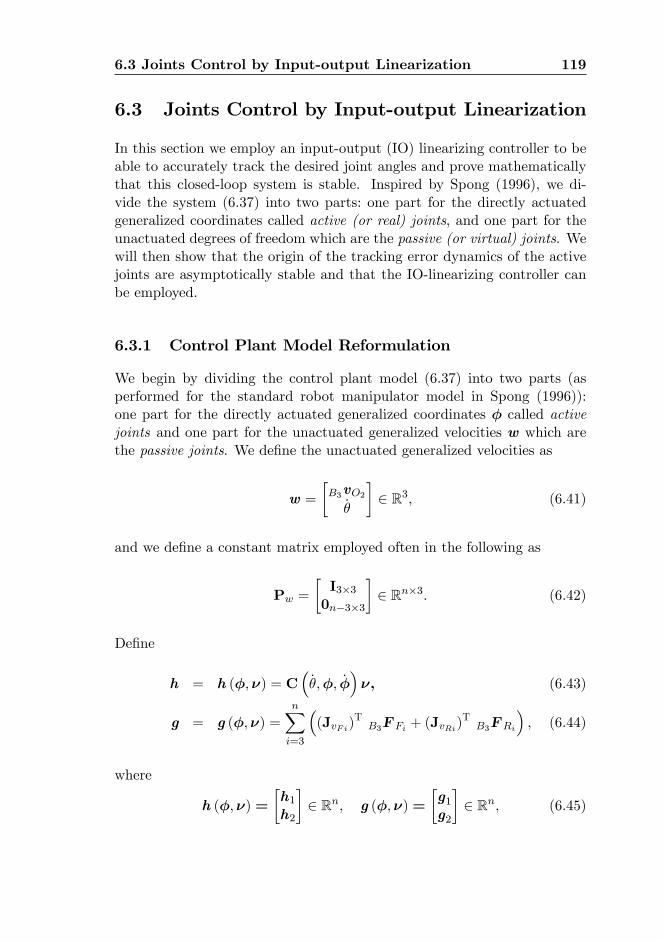
6.3 Joints Control by Input-output Linearization 119
6.3 Joints Control by Input-output Linearization
In this section we employ an input-output (IO) linearizing controller to beable to accurately track the desired joint angles and prove mathematicallythat this closed-loop system is stable. Inspired by Spong (1996), we di-vide the system (6.37) into two parts: one part for the directly actuatedgeneralized coordinates called active (or real) joints, and one part for theunactuated degrees of freedom which are the passive (or virtual) joints. Wewill then show that the origin of the tracking error dynamics of the activejoints are asymptotically stable and that the IO-linearizing controller canbe employed.
6.3.1 Control Plant Model Reformulation
We begin by dividing the control plant model (6.37) into two parts (asperformed for the standard robot manipulator model in Spong (1996)):one part for the directly actuated generalized coordinates � called activejoints and one part for the unactuated generalized velocities w which arethe passive joints. We de�ne the unactuated generalized velocities as
w =
�B3vO2_�
�2 R3; (6.41)
and we de�ne a constant matrix employed often in the following as
Pw =
�I3�30n�3�3
�2 Rn�3: (6.42)
De�ne
h = h (�;�) = C�_�;�; _�
��; (6.43)
g = g (�;�) =nXi=3
�(JvFi)
TB3F Fi + (JvRi)
TB3FRi
�; (6.44)
where
h (�;�) =
�h1h2
�2 Rn; g (�;�) =
�g1g2
�2 Rn; (6.45)
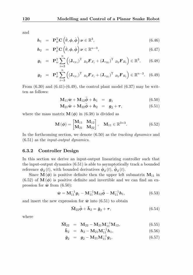
120 Modelling and Control of a Planar Snake Robot
and
h1 = PTwC�_�;�; _�
�� 2 R3; (6.46)
h2 = PT�C�_�;�; _�
�� 2 Rn�3; (6.47)
g1 = PTw
nXi=3
�(JvFi)
TB3F Fi + (JvRi)
TB3FRi
�2 R3; (6.48)
g2 = PT�
nXi=3
�(JvFi)
TB3F Fi + (JvRi)
TB3FRi
�2 Rn�3: (6.49)
From (6.30) and (6.41)-(6.49), the control plant model (6.37) may be writ-ten as follows:
M11 _w +M12��+ h1 = g1 (6.50)
M21 _w +M22��+ h2 = g2 + � ; (6.51)
where the mass matrix M (�) in (6.38) is divided as
M (�) =
�M11 M12
M21 M22
�; M11 2 R3�3: (6.52)
In the forthcoming section, we denote (6.50) as the tracking dynamics and(6.51) as the input-output dynamics.
6.3.2 Controller Design
In this section we derive an input-output linearizing controller such thatthe input-output dynamics (6.51) is able to asymptotically track a boundedreference �d (t), with bounded derivatives _�d (t), ��d (t).
Since M (�) is positive de�nite then the upper left submatrix M11 in(6.52) of M (�) is positive de�nite and invertible and we can �nd an ex-pression for _w from (6.50):
_w =M�111 g1 �M
�111M12
���M�111 h1; (6.53)
and insert the new expression for _w into (6.51) to obtain
�M22��+ �h2 = �g2 + � ; (6.54)
where
�M22 = M22 �M21M�111M12; (6.55)
�h2 = h2 �M21M�111 h1; (6.56)
�g2 = g2 �M21M�111 g1; (6.57)
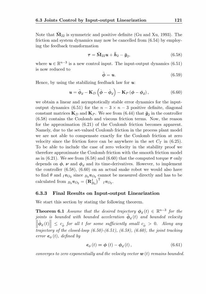
6.3 Joints Control by Input-output Linearization 121
Note that �M22 is symmetric and positive de�nite (Gu and Xu, 1993). Thefriction and system dynamics may now be cancelled from (6.54) by employ-ing the feedback transformation
� = �M22u+ �h2 � �g2; (6.58)
where u 2 Rn�3 is a new control input. The input-output dynamics (6.51)is now reduced to
�� = u: (6.59)
Hence, by using the stabilizing feedback law for u:
u = ��d �KD
�_�� _�d
��KP (�� �d) ; (6.60)
we obtain a linear and asymptotically stable error dynamics for the input-output dynamics (6.51) for the n � 3 � n � 3 positive de�nite, diagonalconstant matricesKD andKP . We see from (6.44) that �g2 in the controller(6.58) contains the Coulomb and viscous friction terms. Now, the reasonfor the approximation (6.21) of the Coulomb friction becomes apparent.Namely, due to the set-valued Coulomb friction in the process plant modelwe are not able to compensate exactly for the Coulomb friction at zerovelocity since the friction force can be anywhere in the set CT in (6.25).To be able to include the case of zero velocity in the stability proof wetherefore approximate the Coulomb friction with the smooth friction modelas in (6.21). We see from (6.58) and (6.60) that the computed torque � onlydepends on �, � and �d and its time-derivatives. However, to implementthe controller (6.58), (6.60) on an actual snake robot we would also haveto �nd � and IvO2 since B3vO2 cannot be measured directly and has to becalculated from B3vO2 =
�RIB3
�TIvO2 .
6.3.3 Final Results on Input-output Linearization
We start this section by stating the following theorem.
Theorem 6.1 Assume that the desired trajectory �d (t) 2 Rn�3 for thejoints is bounded with bounded acceleration ��d (t) and bounded velocity _�d (t) � c _� for all t for some su¢ ciently small c _� > 0. Along any
trajectory of the closed-loop (6.50)-(6.51), (6.58), (6.60), the joint trackingerror e� (t), de�ned by
e� (t) = � (t)� �d (t) ; (6.61)
converges to zero exponentially and the velocity vector w (t) remains bounded.
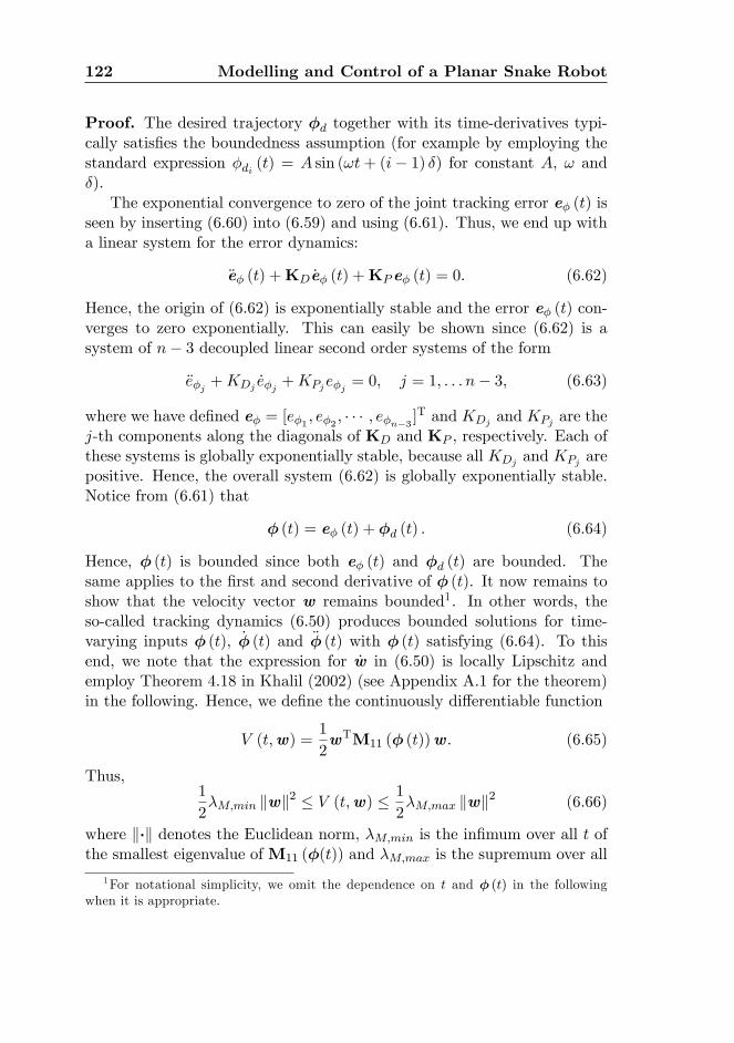
122 Modelling and Control of a Planar Snake Robot
Proof. The desired trajectory �d together with its time-derivatives typi-cally satis�es the boundedness assumption (for example by employing thestandard expression �di (t) = A sin (!t+ (i� 1) �) for constant A, ! and�).
The exponential convergence to zero of the joint tracking error e� (t) isseen by inserting (6.60) into (6.59) and using (6.61). Thus, we end up witha linear system for the error dynamics:
�e� (t) +KD _e� (t) +KPe� (t) = 0: (6.62)
Hence, the origin of (6.62) is exponentially stable and the error e� (t) con-verges to zero exponentially. This can easily be shown since (6.62) is asystem of n� 3 decoupled linear second order systems of the form
�e�j +KDj _e�j +KPje�j = 0; j = 1; : : : n� 3; (6.63)
where we have de�ned e� = [e�1 ; e�2 ; � � � ; e�n�3 ]T and KDj and KPj are the
j-th components along the diagonals of KD and KP , respectively. Each ofthese systems is globally exponentially stable, because all KDj and KPj arepositive. Hence, the overall system (6.62) is globally exponentially stable.Notice from (6.61) that
� (t) = e� (t) + �d (t) : (6.64)
Hence, � (t) is bounded since both e� (t) and �d (t) are bounded. Thesame applies to the �rst and second derivative of � (t). It now remains toshow that the velocity vector w remains bounded1. In other words, theso-called tracking dynamics (6.50) produces bounded solutions for time-varying inputs � (t), _� (t) and �� (t) with � (t) satisfying (6.64). To thisend, we note that the expression for _w in (6.50) is locally Lipschitz andemploy Theorem 4.18 in Khalil (2002) (see Appendix A.1 for the theorem)in the following. Hence, we de�ne the continuously di¤erentiable function
V (t;w) =1
2wTM11 (� (t))w: (6.65)
Thus,1
2�M;min kwk2 � V (t;w) � 1
2�M;max kwk2 (6.66)
where k�k denotes the Euclidean norm, �M;min is the in�mum over all t ofthe smallest eigenvalue ofM11 (�(t)) and �M;max is the supremum over all
1For notational simplicity, we omit the dependence on t and � (t) in the followingwhen it is appropriate.
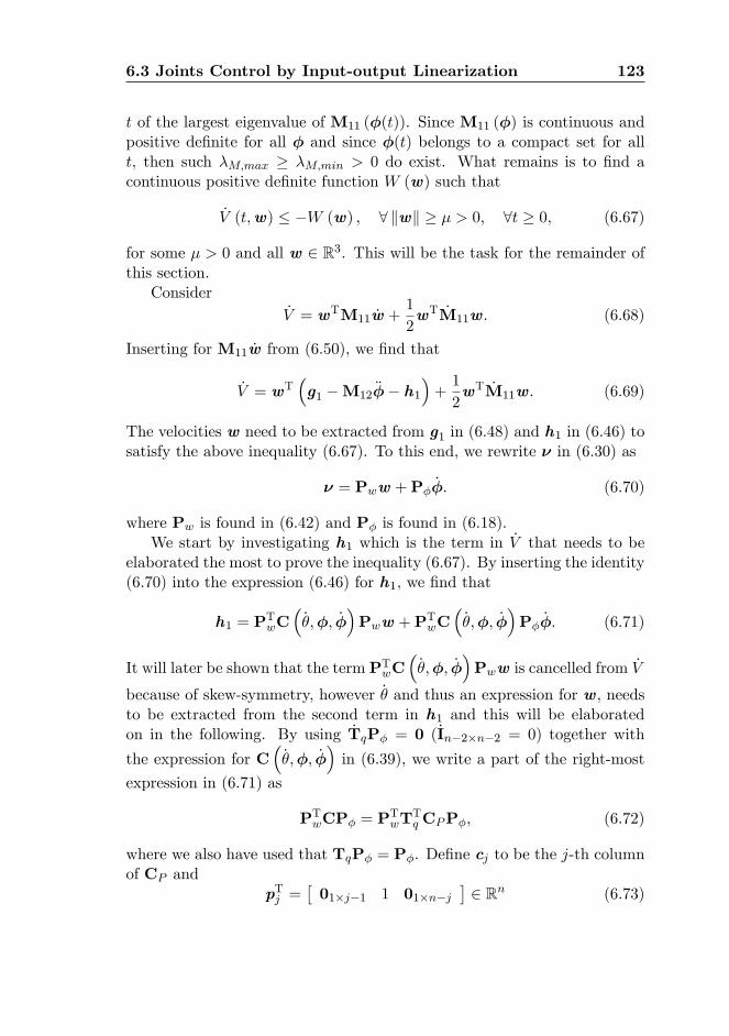
6.3 Joints Control by Input-output Linearization 123
t of the largest eigenvalue of M11 (�(t)). Since M11 (�) is continuous andpositive de�nite for all � and since �(t) belongs to a compact set for allt, then such �M;max � �M;min > 0 do exist. What remains is to �nd acontinuous positive de�nite function W (w) such that
_V (t;w) � �W (w) ; 8 kwk � � > 0; 8t � 0; (6.67)
for some � > 0 and all w 2 R3. This will be the task for the remainder ofthis section.
Consider_V = wTM11 _w +
1
2wT _M11w: (6.68)
Inserting for M11 _w from (6.50), we �nd that
_V = wT�g1 �M12
��� h1�+1
2wT _M11w: (6.69)
The velocities w need to be extracted from g1 in (6.48) and h1 in (6.46) tosatisfy the above inequality (6.67). To this end, we rewrite � in (6.30) as
� = Pww +P� _�: (6.70)
where Pw is found in (6.42) and P� is found in (6.18).We start by investigating h1 which is the term in _V that needs to be
elaborated the most to prove the inequality (6.67). By inserting the identity(6.70) into the expression (6.46) for h1, we �nd that
h1 = PTwC
�_�;�; _�
�Pww +P
TwC
�_�;�; _�
�P� _�: (6.71)
It will later be shown that the term PTwC�_�;�; _�
�Pww is cancelled from _V
because of skew-symmetry, however _� and thus an expression for w, needsto be extracted from the second term in h1 and this will be elaboratedon in the following. By using _TqP� = 0 (_In�2�n�2 = 0) together with
the expression for C�_�;�; _�
�in (6.39), we write a part of the right-most
expression in (6.71) as
PTwCP� = PTwT
Tq CPP�; (6.72)
where we also have used that TqP� = P�. De�ne cj to be the j-th columnof CP and
pTj =�01�j�1 1 01�n�j
�2 Rn (6.73)
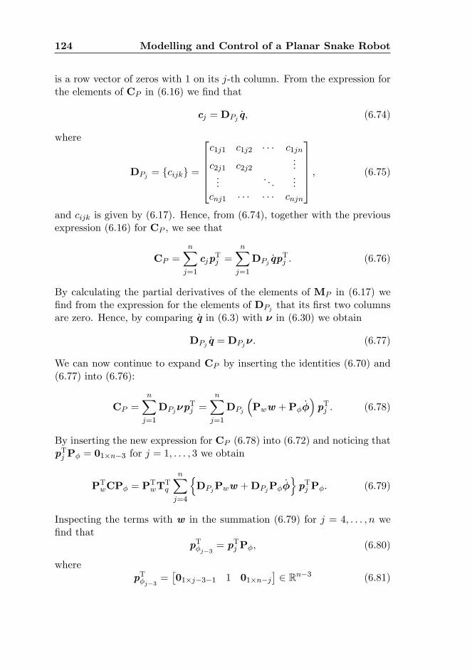
124 Modelling and Control of a Planar Snake Robot
is a row vector of zeros with 1 on its j-th column. From the expression forthe elements of CP in (6.16) we �nd that
cj = DPj _q; (6.74)
where
DPj = fcijkg =
266664c1j1 c1j2 � � � c1jn
c2j1 c2j2...
.... . .
...cnj1 � � � � � � cnjn
377775 ; (6.75)
and cijk is given by (6.17). Hence, from (6.74), together with the previousexpression (6.16) for CP , we see that
CP =nXj=1
cjpTj =
nXj=1
DPj _qpTj : (6.76)
By calculating the partial derivatives of the elements of MP in (6.17) we�nd from the expression for the elements of DPj that its �rst two columnsare zero. Hence, by comparing _q in (6.3) with � in (6.30) we obtain
DPj _q = DPj�: (6.77)
We can now continue to expand CP by inserting the identities (6.70) and(6.77) into (6.76):
CP =nXj=1
DPj�pTj =
nXj=1
DPj
�Pww +P� _�
�pTj : (6.78)
By inserting the new expression for CP (6.78) into (6.72) and noticing thatpTj P� = 01�n�3 for j = 1; : : : ; 3 we obtain
PTwCP� = PTwT
Tq
nXj=4
nDPjPww +DPjP�
_�opTj P�: (6.79)
Inspecting the terms with w in the summation (6.79) for j = 4; : : : ; n we�nd that
pT�j�3 = pTj P�; (6.80)
wherepT�j�3 =
�01�j�3�1 1 01�n�j
�2 Rn�3 (6.81)
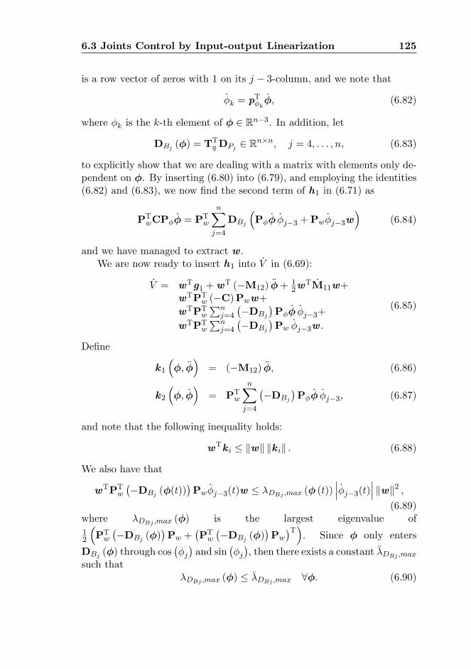
6.3 Joints Control by Input-output Linearization 125
is a row vector of zeros with 1 on its j � 3-column, and we note that
_�k = pT�k_�; (6.82)
where �k is the k-th element of � 2 Rn�3. In addition, let
DBj (�) = TTqDPj 2 Rn�n; j = 4; : : : ; n; (6.83)
to explicitly show that we are dealing with a matrix with elements only de-pendent on �. By inserting (6.80) into (6.79), and employing the identities(6.82) and (6.83), we now �nd the second term of h1 in (6.71) as
PTwCP�_� = PTw
nXj=4
DBj
�P� _� _�j�3 +Pw _�j�3w
�(6.84)
and we have managed to extract w.We are now ready to insert h1 into _V in (6.69):
_V = wTg1 +wT (�M12) ��+
12w
T _M11w+wTPTw (�C)Pww+wTPTw
Pnj=4
��DBj
�P� _� _�j�3+
wTPTwPn
j=4
��DBj
�Pw _�j�3w:
(6.85)
De�ne
k1
��; ��
�= (�M12) ��; (6.86)
k2
��; _�
�= PTw
nXj=4
��DBj
�P� _� _�j�3; (6.87)
and note that the following inequality holds:
wTki � kwk kkik : (6.88)
We also have that
wTPTw��DBj (�(t))
�Pw _�j�3(t)w � �DBj ;max (� (t))
��� _�j�3(t)��� kwk2 ;(6.89)
where �DBj ;max (�) is the largest eigenvalue of12
�PTw��DBj (�)
�Pw +
�PTw��DBj (�)
�Pw�T�. Since � only enters
DBj (�) through cos��j�and sin
��j�, then there exists a constant ��DBj ;max
such that�DBj ;max (�) � ��DBj ;max 8�: (6.90)
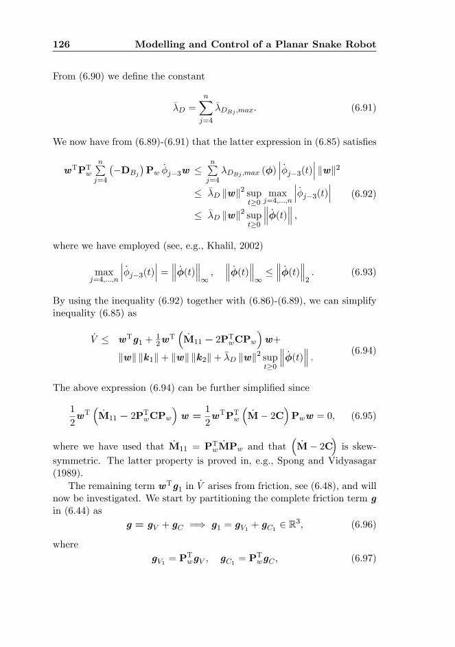
126 Modelling and Control of a Planar Snake Robot
From (6.90) we de�ne the constant
��D =nXj=4
��DBj ;max: (6.91)
We now have from (6.89)-(6.91) that the latter expression in (6.85) satis�es
wTPTwnPj=4
��DBj
�Pw _�j�3w �
nPj=4
�DBj ;max (�)��� _�j�3(t)��� kwk2
� ��D kwk2 supt�0
maxj=4;:::;n
��� _�j�3(t)���� ��D kwk2 sup
t�0
_�(t) ;(6.92)
where we have employed (see, e.g., Khalil, 2002)
maxj=4;:::;n
��� _�j�3(t)��� = _�(t) 1 ; _�(t)
1� _�(t)
2: (6.93)
By using the inequality (6.92) together with (6.86)-(6.89), we can simplifyinequality (6.85) as
_V � wTg1 +12w
T�_M11 � 2PTwCPw
�w+
kwk kk1k+ kwk kk2k+ ��D kwk2 supt�0
_�(t) : (6.94)
The above expression (6.94) can be further simpli�ed since
1
2wT
�_M11 � 2PTwCPw
�w =
1
2wTPTw
�_M� 2C
�Pww = 0; (6.95)
where we have used that _M11 = PTw_MPw and that
�_M� 2C
�is skew-
symmetric. The latter property is proved in, e.g., Spong and Vidyasagar(1989).
The remaining term wTg1 in _V arises from friction, see (6.48), and willnow be investigated. We start by partitioning the complete friction term gin (6.44) as
g = gV + gC =) g1 = gV1 + gC1 2 R3; (6.96)
wheregV1 = P
TwgV ; gC1 = P
TwgC ; (6.97)
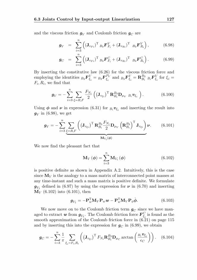
6.3 Joints Control by Input-output Linearization 127
and the viscous friction gV and Coulomb friction gC are
gV =nXi=3
�(JvFi)
TB3F
VFi + (JvRi)
TB3F
VRi
�; (6.98)
gC =nXi=3
�(JvFi)
TB3F
CFi + (JvRi)
TB3F
CRi
�: (6.99)
By inserting the constitutive law (6.26) for the viscous friction force andemploying the identities B3F
V�i= B3F
PV�iand B3F
V�i= RB3
Bi BiFV�ifor �i =
Fi; Ri, we �nd that
gV = �nXi=3
X�=R;F
FNi2
��Jv�i
�TRB3BiD�V Biv�i
�: (6.100)
Using � and � in expression (6.31) for Biv�i and inserting the result intogV in (6.98), we get
gV = �nXi=3
X�=R;F
��Jv�i
�TRB3Bi
FNi2D�V
�RB3Bi
�TJv�i
�| {z }
MVi(�)
�: (6.101)
We now �nd the pleasant fact that
MV (�) =nXi=3
MVi (�) (6.102)
is positive de�nite as shown in Appendix A.2. Intuitively, this is the casesinceMV is the analogy to a mass matrix of interconnected point masses atany time-instant and such a mass matrix is positive de�nite. We formulategV1 de�ned in (6.97) by using the expression for � in (6.70) and insertingMV (6.102) into (6.101), then
gV1 = �PTwMVPww �PTwMVP� _�: (6.103)
We now move on to the Coulomb friction term gC since we have man-aged to extract w from gV1 . The Coulomb friction force F
C�iis found as the
smooth approximation of the Coulomb friction force in (6.21) on page 115and by inserting this into the expression for gC in (6.99), we obtain
gC = �nXi=3
1
�
X�i=Fi;Ri
��Jv�i
�TFNiR
B3BiD�C arctan
�Biv�i�C
��: (6.104)
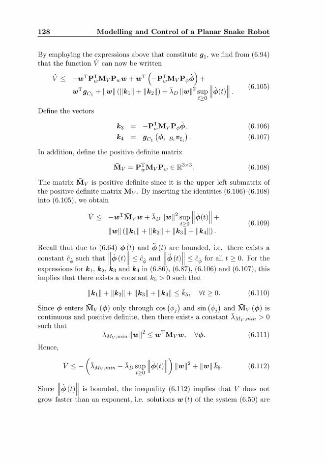
128 Modelling and Control of a Planar Snake Robot
By employing the expressions above that constitute g1, we �nd from (6.94)that the function _V can now be written
_V � �wTPTwMVPww +wT��PTwMVP� _�
�+
wTgC1 + kwk (kk1k+ kk2k) + ��D kwk2 supt�0
_�(t) : (6.105)
De�ne the vectors
k3 = �PTwMVP� _�; (6.106)
k4 = gC1��; Biv�i
�: (6.107)
In addition, de�ne the positive de�nite matrix
�MV = PTwMVPw 2 R3�3: (6.108)
The matrix �MV is positive de�nite since it is the upper left submatrix ofthe positive de�nite matrixMV . By inserting the identities (6.106)-(6.108)into (6.105), we obtain
_V � �wT �MVw + ��D kwk2 supt�0
_�(t) +kwk (kk1k+ kk2k+ kk3k+ kk4k) :
(6.109)
Recall that due to (6.64) _� (t) and �� (t) are bounded, i.e. there exists a
constant ~c _� such that _� (t) � ~c _� and �� (t) � ~c _� for all t � 0. For the
expressions for k1, k2, k3 and k4 in (6.86), (6.87), (6.106) and (6.107), thisimplies that there exists a constant �k5 > 0 such that
kk1k+ kk2k+ kk3k+ kk4k � �k5; 8t � 0: (6.110)
Since � enters �MV (�) only through cos��j�and sin
��j�and �MV (�) is
continuous and positive de�nite, then there exists a constant ��MV ;min > 0such that
��MV ;min kwk2 � wT �MVw; 8�: (6.111)
Hence,
_V � ����MV ;min � ��D sup
t�0
_�(t) � kwk2 + kwk �k5: (6.112)
Since _� (t) is bounded, the inequality (6.112) implies that V does not
grow faster than an exponent, i.e. solutions w (t) of the system (6.50) are
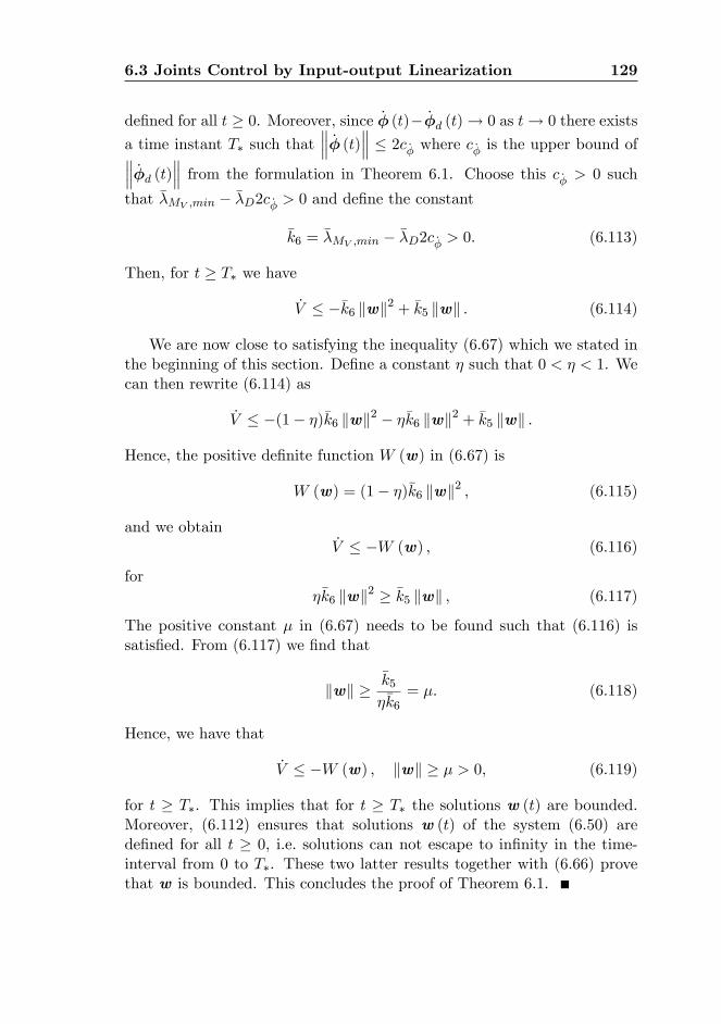
6.3 Joints Control by Input-output Linearization 129
de�ned for all t � 0. Moreover, since _� (t)� _�d (t)! 0 as t! 0 there exists
a time instant T� such that _� (t) � 2c _� where c _� is the upper bound of _�d (t) from the formulation in Theorem 6.1. Choose this c _� > 0 such
that ��MV ;min � ��D2c _� > 0 and de�ne the constant
�k6 = ��MV ;min � ��D2c _� > 0: (6.113)
Then, for t � T� we have
_V � ��k6 kwk2 + �k5 kwk : (6.114)
We are now close to satisfying the inequality (6.67) which we stated inthe beginning of this section. De�ne a constant � such that 0 < � < 1. Wecan then rewrite (6.114) as
_V � �(1� �)�k6 kwk2 � ��k6 kwk2 + �k5 kwk :
Hence, the positive de�nite function W (w) in (6.67) is
W (w) = (1� �)�k6 kwk2 ; (6.115)
and we obtain_V � �W (w) ; (6.116)
for��k6 kwk2 � �k5 kwk ; (6.117)
The positive constant � in (6.67) needs to be found such that (6.116) issatis�ed. From (6.117) we �nd that
kwk ��k5��k6
= �: (6.118)
Hence, we have that
_V � �W (w) ; kwk � � > 0; (6.119)
for t � T�. This implies that for t � T� the solutions w (t) are bounded.Moreover, (6.112) ensures that solutions w (t) of the system (6.50) arede�ned for all t � 0, i.e. solutions can not escape to in�nity in the time-interval from 0 to T�. These two latter results together with (6.66) provethat w is bounded. This concludes the proof of Theorem 6.1.
130 Modelling and Control of a Planar Snake Robot
6.4 Summary
This chapter considers the problem of model-based control of the joints of asnake robot without wheels. The potential range of applications of snake ro-bots is wide and delicate operations such as inspection and maintenance inindustrial environments or performing search and rescue operations requireprecise control of snake robot joints. To this end, we present a controllerthat asymptotically stabilizes the joints of the snake robot to a desired refer-ence trajectory. We have developed a planar model of the snake robot basedon the standard dynamics of a robot manipulator. This model is denotedthe process plant model. Such a formulation is advantageous for controlsince it allows us to employ the large variety of control techniques availablefor robot manipulators. Our controller is based on input-output lineariza-tion of a control plant model, which is a reformulation of the process plantmodel, of the snake robot dynamics also developed in this chapter. Thereformulation of the process plant model is necessary to make the stabilityanalysis more manageable and exponential stability of the desired trajec-tories for the joints is shown with a formal Lyapunov-based stability proof.The performance of the controller will be tested in simulation on both asmooth and non-smooth planar snake robot model in Chapter 7.
Chapter 7
Simulation andExperimental Results
7.1 Introduction
The ability to investigate a system by simulation, as opposed to testing theactual system, is a powerful tool for testing and evaluating the system aslong as the model represents the actual system dynamics with su¢ cientlyhigh accuracy. In general, simulations allow one to evaluate the systemwithout risking damaging it or wearing it out. In addition, it is easier totry out various initial conditions since the actual system does not need tobe manipulated for each trial.
In this chapter we present simulations of the various snake robot modelspresented throughout this thesis. The algorithms for the time-steppingmethod presented for the 2D and 3D model have been implemented fornumerical treatment of the models and we investigate whether the time-stepping method is suitable for simulating the models. We have qualitativeknowledge from previously published papers on snake robots of how a snakerobot should perform during various motion patterns. In this chapter wewill test a selection of these gaits to see whether the snake robot movesas expected with our models. Moreover, to further validate the model,experimental results will be presented for the NTNU/SINTEF snake robot�Aiko� and these results will be compared to the simulation results fromboth the 2D model presented in Chapter 3 and the 3D model presented inChapter 4. We will also investigate how the 2D and 3D model performs forobstacle aided locomotion with small obstacles. Such small obstacles may,in general, cause problems due to numerical issues and that the obstacles
132 Simulation and Experimental Results
may get stuck in the snake robot due to the design of the exterior of thesnake robot. In addition, the 3D model will be tested for a motion patternbased on rolling to motivate the inclusion of the exoskeleton de�ned forcontact with the ground surface. Moreover, the input-output linearizingcontroller presented in Chapter 6 will be evaluated for an idealized snakerobot model and for a model that includes various degrees of noise. Theseresults will be compared to an ordinary PD-controller. Both of these lattermodels are based on the �robot model�developed in Chapter 6.
This chapter includes the results from Transeth et al. (2007a), Transethet al. (2008b) and Transeth et al. (2008a) and it is organized as follows.A snake robot called �Aiko�� the basis for the models � is presented inSection 7.2 together with all simulation parameters. Simulation results aregiven in Section 7.3. The experimental setup is presented in Section 7.4and simulations with back-to-back comparisons to experimental results aregiven in Section 7.5. A summary of the most important �ndings in thischapter is given in Section 7.6.
7.2 Simulation Parameters
The snake robot �Aiko�is used as a basis for the mathematical models. Inthis section we will describe the most important characteristics of the snakerobot and use these to determine the parameters for the models presented inChapters 3, 4 and 6. In addition, we will present the simulation parameters.
7.2.1 A Description of Aiko and Model Parameters
Aiko is depicted in Figure 7.1 and has eleven (red) links connected by tentwo DOF joints. As seen from the �gure, the snake robot has cylindri-cal links and a half-sphere made of metal as a �head�which may be re-moved. Aiko weighs 7.5 kg and each link is 12.2 cm long. The snake robotwas developed1 at the NTNU/SINTEF Advanced Robotics Laboratory inTrondheim, Norway in the year 2006.
1General requirements for Aiko were formulated by Pål Liljebäck and Aksel AndreasTranseth. These requirements included that the snake robot should have 2 DOF joints, beable to lift three or more of its links and have an as smooth as possible exoskeleton to beable to use obstacles to move forward and/or move over them. Moreover, the exoskeletonshould be cylindrical to be able to easily move by e.g. lateral rolling. Sverre Brovolland Kristo¤er Nyborg Gregertsen developed Aiko based on these requirements duringS. Brovoll�s Master�s degree and K. N. Gregertsen�s summer job at SINTEF under thesupervision of P. Liljebäck, A. A. Transeth and Amund Skavhaug. A detailed descriptionof the design and components of Aiko is found in Brovoll (2006).
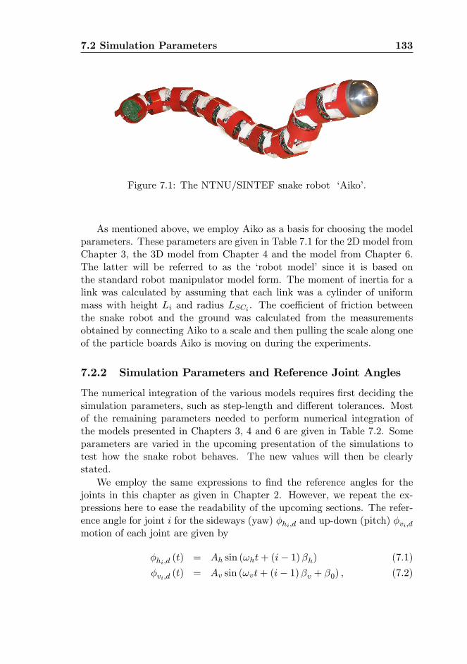
7.2 Simulation Parameters 133
Figure 7.1: The NTNU/SINTEF snake robot �Aiko�.
As mentioned above, we employ Aiko as a basis for choosing the modelparameters. These parameters are given in Table 7.1 for the 2D model fromChapter 3, the 3D model from Chapter 4 and the model from Chapter 6.The latter will be referred to as the �robot model� since it is based onthe standard robot manipulator model form. The moment of inertia for alink was calculated by assuming that each link was a cylinder of uniformmass with height Li and radius LSCi . The coe¢ cient of friction betweenthe snake robot and the ground was calculated from the measurementsobtained by connecting Aiko to a scale and then pulling the scale along oneof the particle boards Aiko is moving on during the experiments.
7.2.2 Simulation Parameters and Reference Joint Angles
The numerical integration of the various models requires �rst deciding thesimulation parameters, such as step-length and di¤erent tolerances. Mostof the remaining parameters needed to perform numerical integration ofthe models presented in Chapters 3, 4 and 6 are given in Table 7.2. Someparameters are varied in the upcoming presentation of the simulations totest how the snake robot behaves. The new values will then be clearlystated.
We employ the same expressions to �nd the reference angles for thejoints in this chapter as given in Chapter 2. However, we repeat the ex-pressions here to ease the readability of the upcoming sections. The refer-ence angle for joint i for the sideways (yaw) �hi;d and up-down (pitch) �vi;dmotion of each joint are given by
�hi;d (t) = Ah sin (!ht+ (i� 1)�h) (7.1)
�vi;d (t) = Av sin (!vt+ (i� 1)�v + �0) ; (7.2)
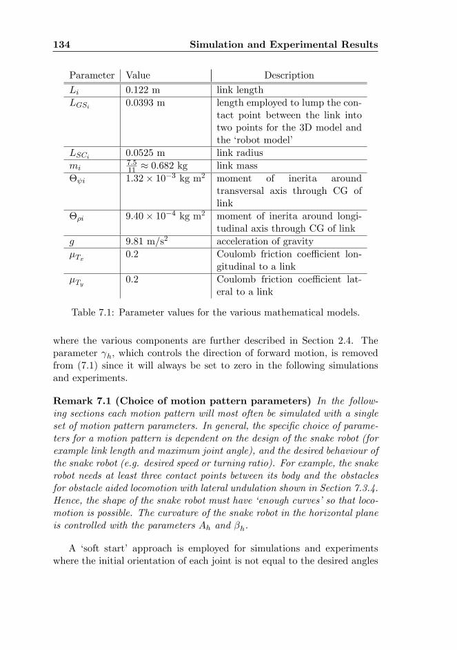
134 Simulation and Experimental Results
Parameter Value Description
Li 0:122 m link lengthLGSi 0:0393 m length employed to lump the con-
tact point between the link intotwo points for the 3D model andthe �robot model�
LSCi 0:0525 m link radiusmi
7:511 � 0:682 kg link mass
� i 1:32� 10�3 kg m2 moment of inerita aroundtransversal axis through CG oflink
��i 9:40� 10�4 kg m2 moment of inerita around longi-tudinal axis through CG of link
g 9:81 m/s2 acceleration of gravity�Tx 0:2 Coulomb friction coe¢ cient lon-
gitudinal to a link�Ty 0:2 Coulomb friction coe¢ cient lat-
eral to a link
Table 7.1: Parameter values for the various mathematical models.
where the various components are further described in Section 2.4. Theparameter h, which controls the direction of forward motion, is removedfrom (7.1) since it will always be set to zero in the following simulationsand experiments.
Remark 7.1 (Choice of motion pattern parameters) In the follow-ing sections each motion pattern will most often be simulated with a singleset of motion pattern parameters. In general, the speci�c choice of parame-ters for a motion pattern is dependent on the design of the snake robot (forexample link length and maximum joint angle), and the desired behaviour ofthe snake robot (e.g. desired speed or turning ratio). For example, the snakerobot needs at least three contact points between its body and the obstaclesfor obstacle aided locomotion with lateral undulation shown in Section 7.3.4.Hence, the shape of the snake robot must have �enough curves�so that loco-motion is possible. The curvature of the snake robot in the horizontal planeis controlled with the parameters Ah and �h.
A �soft start� approach is employed for simulations and experimentswhere the initial orientation of each joint is not equal to the desired angles
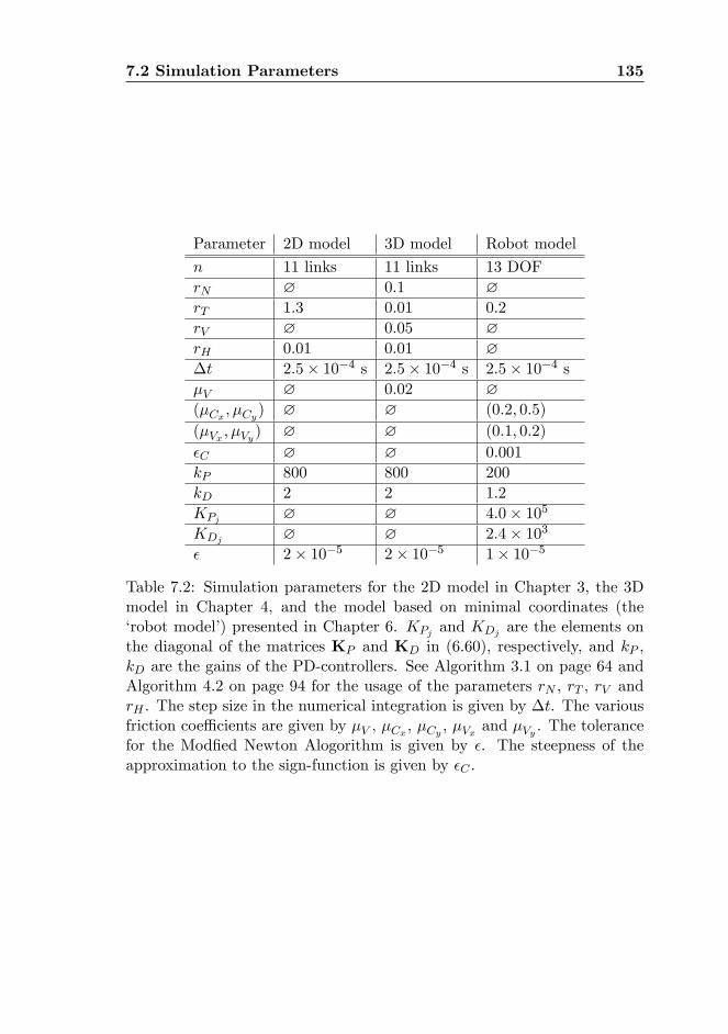
7.2 Simulation Parameters 135
Parameter 2D model 3D model Robot model
n 11 links 11 links 13 DOFrN ? 0:1 ?rT 1:3 0:01 0:2
rV ? 0:05 ?rH 0:01 0:01 ?�t 2:5� 10�4 s 2:5� 10�4 s 2:5� 10�4 s�V ? 0:02 ?(�Cx ; �Cy) ? ? (0:2; 0:5)
(�Vx ; �Vy) ? ? (0:1; 0:2)
�C ? ? 0:001
kP 800 800 200
kD 2 2 1:2
KPj ? ? 4:0� 105KDj ? ? 2:4� 103� 2� 10�5 2� 10�5 1� 10�5
Table 7.2: Simulation parameters for the 2D model in Chapter 3, the 3Dmodel in Chapter 4, and the model based on minimal coordinates (the�robot model�) presented in Chapter 6. KPj and KDj are the elements onthe diagonal of the matrices KP and KD in (6.60), respectively, and kP ,kD are the gains of the PD-controllers. See Algorithm 3.1 on page 64 andAlgorithm 4.2 on page 94 for the usage of the parameters rN , rT , rV andrH . The step size in the numerical integration is given by �t. The variousfriction coe¢ cients are given by �V , �Cx , �Cy , �Vx and �Vy . The tolerancefor the Mod�ed Newton Alogorithm is given by �. The steepness of theapproximation to the sign-function is given by �C .
136 Simulation and Experimental Results
�hi;d (t) and �vi;d (t) at the time the snake robot is started. An example ofsuch a situation is if we want the snake robot to move forward by lateralundulation, but it has a straight posture at t = 0. The �soft start�approachis utilized to avoid large steps in the reference signal which causes largeactuator torques. To this end, we consider all the reference signals �hi;d (t)and �hi;d (t) separately and calculate them from the expressions (7.1) and(7.2) for the reference angles, respectively. However, we set �hi;d (t) = 0until
���hi;d (t)�� � 3�=180 and �vi;d (t) = 0 until ���vi;d (t)�� � 3�=180 for the�rst time after start-up. After the reference value is within the allowedstart value, the reference angle is found from (7.1) or (7.2).
7.3 Simulations without Experimental Validation
In this section we present simulations of the models presented in this the-sis. First, we simulate the 3D model where the snake robot is raised abovethe ground surface and then dropped onto it. This scenario challengesthe numerical stability of the numerical treatment since large sudden con-tact forces arise simultaneously. Moreover, we check whether the snakerobot moves forward by lateral undulation with anisotropic friction, as itis expected to. Second, we test if the de�ned exoskeleton works well for U-shaped lateral rolling and sidewinding, and we investigate what happens ifthe friction between the snake robot and the ground surface is changed forthese motion patterns. Third, obstacle aided locomotion is simulated withsmall obstacles. Such small obstacles pose di¢ culties both in the numericaltreatment and that the snake robot may get stuck. We investigate how our2D and 3D models perform for these challenges and we also enquire intohow the snake robot behaves if one obstacle that is necessary for forwardmotion is moved. Moreover, contact forces between the snake robot andthe obstacles are plotted and compared to the discussion on obstacle aidedlocomotion given in Chapter 5. Finally, the input-output linearizing con-troller is compared to a conventional PD-controller, both implemented onthe �robot model�. In addition to the comparison, we will also inquire intowhether the �robot model�is suitable for numerical treatment. Note thatfor simulation of the 2D model presented in Chapter 3 we always employthe PD-controller given in the same chapter due to its simplicity and sincethe very high accuracy in the control of the snake robot joints o¤ered bythe input-output linearizing controller is not crucial for testing the validityof the 2D model. Moreover, the PD-controllers given for the 3D model fromChapter 4 are always employed when simulating the 3D model.
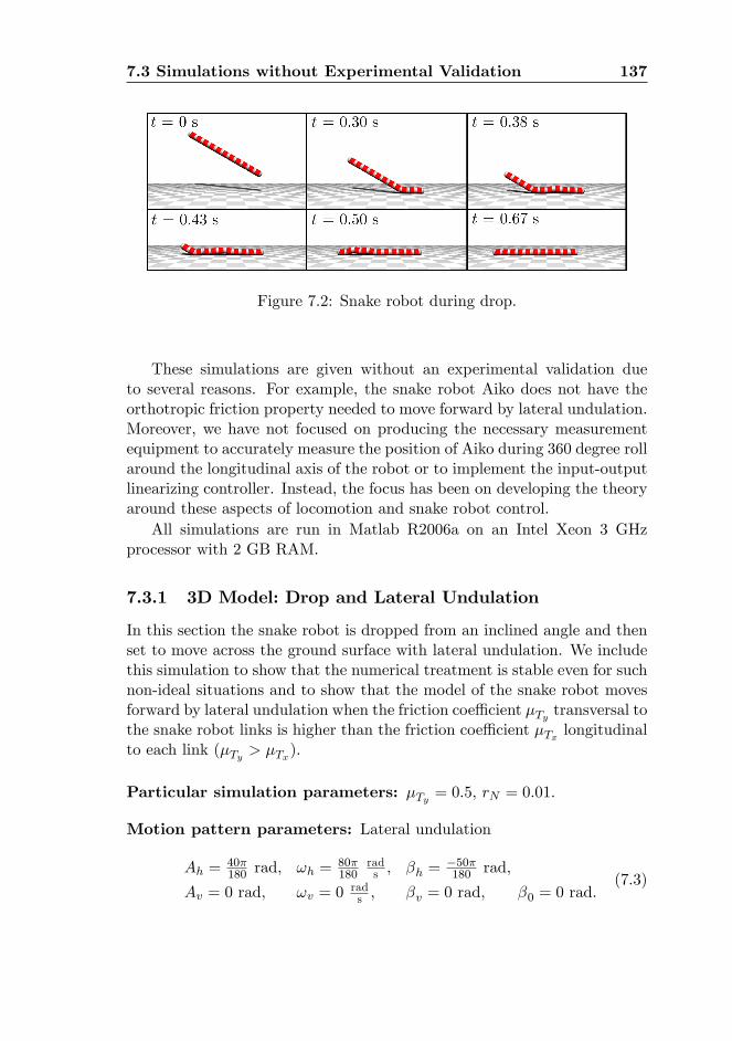
7.3 Simulations without Experimental Validation 137
Figure 7.2: Snake robot during drop.
These simulations are given without an experimental validation dueto several reasons. For example, the snake robot Aiko does not have theorthotropic friction property needed to move forward by lateral undulation.Moreover, we have not focused on producing the necessary measurementequipment to accurately measure the position of Aiko during 360 degree rollaround the longitudinal axis of the robot or to implement the input-outputlinearizing controller. Instead, the focus has been on developing the theoryaround these aspects of locomotion and snake robot control.
All simulations are run in Matlab R2006a on an Intel Xeon 3 GHzprocessor with 2 GB RAM.
7.3.1 3D Model: Drop and Lateral Undulation
In this section the snake robot is dropped from an inclined angle and thenset to move across the ground surface with lateral undulation. We includethis simulation to show that the numerical treatment is stable even for suchnon-ideal situations and to show that the model of the snake robot movesforward by lateral undulation when the friction coe¢ cient �Ty transversal tothe snake robot links is higher than the friction coe¢ cient �Tx longitudinalto each link (�Ty > �Tx).
Particular simulation parameters: �Ty = 0:5, rN = 0:01.
Motion pattern parameters: Lateral undulation
Ah =40�180 rad, !h =
80�180
rads , �h =
�50�180 rad,
Av = 0 rad, !v = 0rads , �v = 0 rad, �0 = 0 rad.
(7.3)
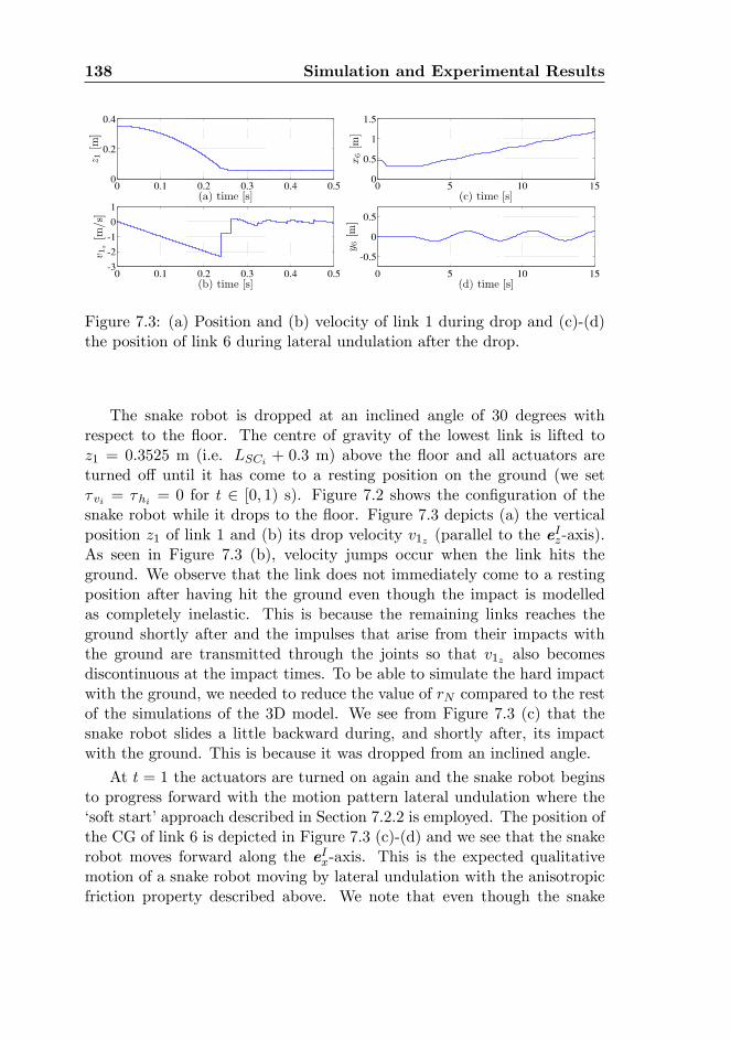
138 Simulation and Experimental Results
Figure 7.3: (a) Position and (b) velocity of link 1 during drop and (c)-(d)the position of link 6 during lateral undulation after the drop.
The snake robot is dropped at an inclined angle of 30 degrees withrespect to the �oor. The centre of gravity of the lowest link is lifted toz1 = 0:3525 m (i.e. LSCi + 0:3 m) above the �oor and all actuators areturned o¤ until it has come to a resting position on the ground (we set� vi = �hi = 0 for t 2 [0; 1) s). Figure 7.2 shows the con�guration of thesnake robot while it drops to the �oor. Figure 7.3 depicts (a) the verticalposition z1 of link 1 and (b) its drop velocity v1z (parallel to the e
Iz-axis).
As seen in Figure 7.3 (b), velocity jumps occur when the link hits theground. We observe that the link does not immediately come to a restingposition after having hit the ground even though the impact is modelledas completely inelastic. This is because the remaining links reaches theground shortly after and the impulses that arise from their impacts withthe ground are transmitted through the joints so that v1z also becomesdiscontinuous at the impact times. To be able to simulate the hard impactwith the ground, we needed to reduce the value of rN compared to the restof the simulations of the 3D model. We see from Figure 7.3 (c) that thesnake robot slides a little backward during, and shortly after, its impactwith the ground. This is because it was dropped from an inclined angle.
At t = 1 the actuators are turned on again and the snake robot beginsto progress forward with the motion pattern lateral undulation where the�soft start�approach described in Section 7.2.2 is employed. The position ofthe CG of link 6 is depicted in Figure 7.3 (c)-(d) and we see that the snakerobot moves forward along the eIx-axis. This is the expected qualitativemotion of a snake robot moving by lateral undulation with the anisotropicfriction property described above. We note that even though the snake
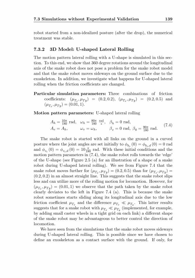
7.3 Simulations without Experimental Validation 139
robot started from a non-idealized posture (after the drop), the numericaltreatment was stable.
7.3.2 3D Model: U-shaped Lateral Rolling
The motion pattern lateral rolling with a U-shape is simulated in this sec-tion. To this end, we show that 360 degree rotations around the longitudinalaxis of the snake robot does not pose a problem for the snake robot modeland that the snake robot moves sideways on the ground surface due to theexoskeleton. In addition, we investigate what happens for U-shaped lateralrolling when the friction coe¢ cients are changed.
Particular simulation parameters: Three combinations of frictioncoe¢ cients: (�Tx ; �Ty) = (0:2; 0:2), (�Tx ; �Ty) = (0:2; 0:5) and(�Tx ; �Ty) = (0:01; 1).
Motion pattern parameters: U-shaped lateral rolling
Ah =10�180 rad, !h =
80�180
rads , �h = 0 rad,
Av = Ah, !v = !h, �v = 0 rad, �0 =90�180 rad.
(7.4)
The snake robot is started with all links on the ground in a curvedposture where the joint angles are set initially to �hi (0) = �hi;d (0) = 0 radand �vi (0) = �vi;d (0) = 10 �
180 rad. With these initial conditions and themotion pattern parameters in (7.4), the snake robot rolls towards the �edge�of the U-shape (see Figure 2.5 (a) for an illustration of a shape of a snakerobot during U-shaped lateral rolling). We see from Figure 7.4 that thesnake robot moves further for (�Tx ; �Ty) = (0:2; 0:5) than for (�Tx ; �Ty) =(0:2; 0:2) in an almost straight line. This suggests that the snake robot slipsless and can utilize more of the rolling motion for locomotion. However, for(�Tx ; �Ty) = (0:01; 1) we observe that the path taken by the snake robotclearly deviates to the left in Figure 7.4 (a). This is because the snakerobot sometimes starts sliding along its longitudinal axis due to the lowfriction coe¢ cient �Tx and the di¤erence �Tx � �Ty . This latter resultssuggests that for a snake robot with �Tx � �Ty (implemented, for example,by adding small caster wheels in a tight grid on each link) a di¤erent shapeof the snake robot may be advantageous to better control the direction oflocomotion.
We have seen from the simulations that the snake robot moves sidewaysduring U-shaped lateral rolling. This is possible since we have chosen tode�ne an exoskeleton as a contact surface with the ground. If only, for
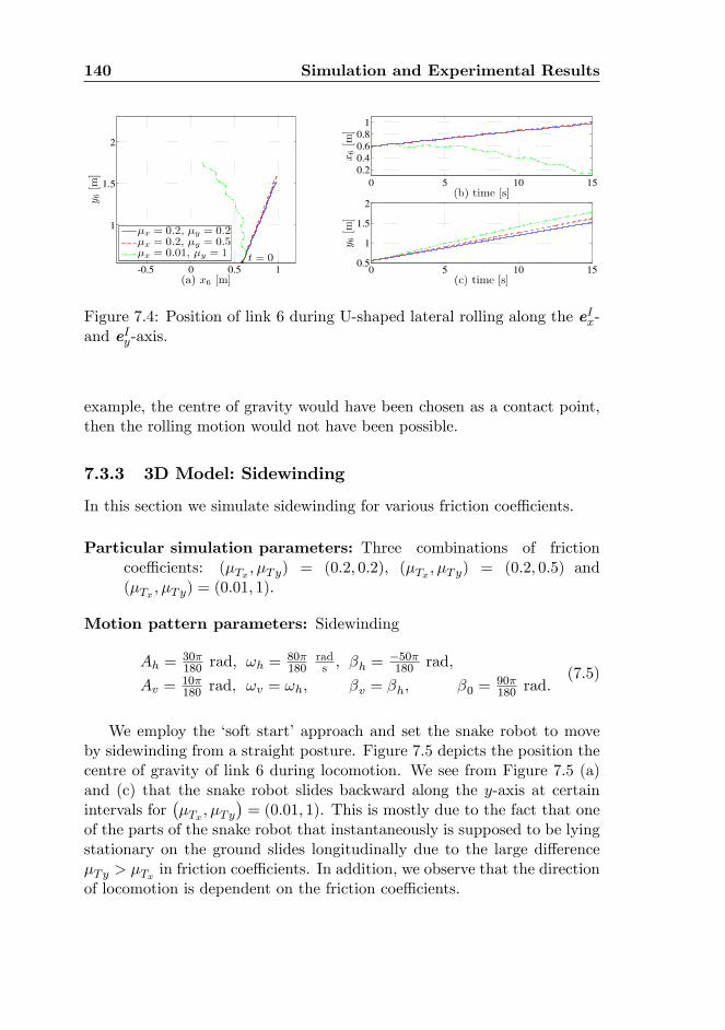
140 Simulation and Experimental Results
Figure 7.4: Position of link 6 during U-shaped lateral rolling along the eIx-and eIy-axis.
example, the centre of gravity would have been chosen as a contact point,then the rolling motion would not have been possible.
7.3.3 3D Model: Sidewinding
In this section we simulate sidewinding for various friction coe¢ cients.
Particular simulation parameters: Three combinations of frictioncoe¢ cients: (�Tx ; �Ty) = (0:2; 0:2), (�Tx ; �Ty) = (0:2; 0:5) and(�Tx ; �Ty) = (0:01; 1).
Motion pattern parameters: Sidewinding
Ah =30�180 rad, !h =
80�180
rads , �h =
�50�180 rad,
Av =10�180 rad, !v = !h, �v = �h, �0 =
90�180 rad.
(7.5)
We employ the �soft start�approach and set the snake robot to moveby sidewinding from a straight posture. Figure 7.5 depicts the position thecentre of gravity of link 6 during locomotion. We see from Figure 7.5 (a)and (c) that the snake robot slides backward along the y-axis at certainintervals for
��Tx ; �Ty
�= (0:01; 1). This is mostly due to the fact that one
of the parts of the snake robot that instantaneously is supposed to be lyingstationary on the ground slides longitudinally due to the large di¤erence�Ty > �Tx in friction coe¢ cients. In addition, we observe that the directionof locomotion is dependent on the friction coe¢ cients.
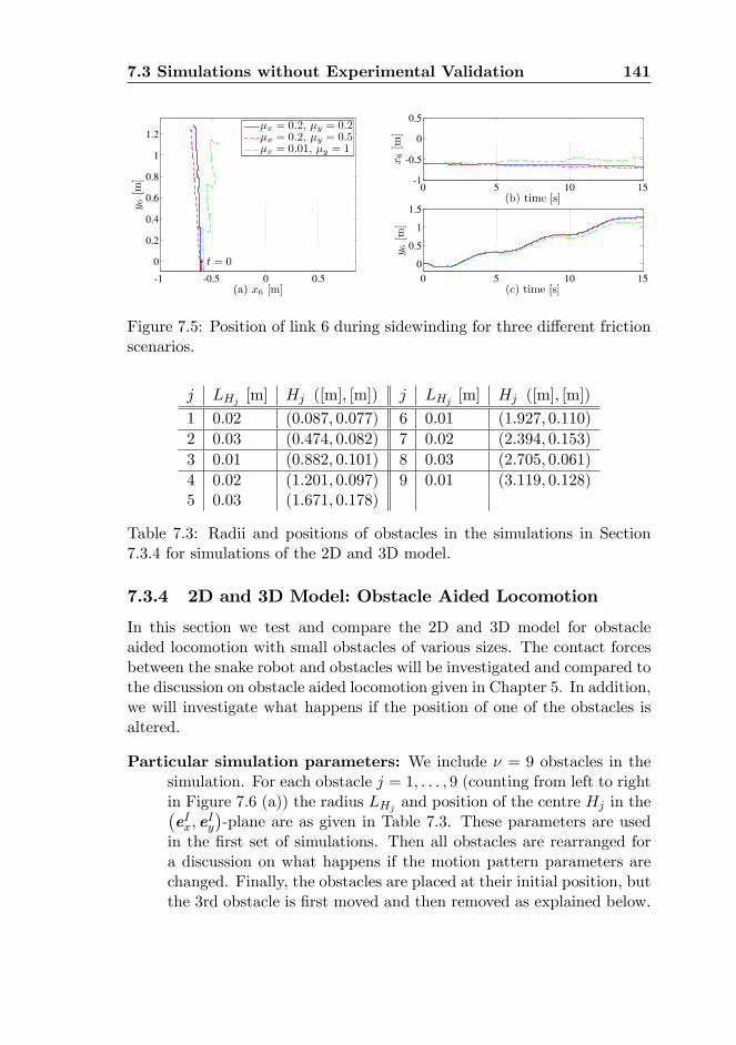
7.3 Simulations without Experimental Validation 141
Figure 7.5: Position of link 6 during sidewinding for three di¤erent frictionscenarios.
j LHj [m] Hj ([m]; [m]) j LHj [m] Hj ([m]; [m])
1 0:02 (0:087; 0:077) 6 0:01 (1:927; 0:110)
2 0:03 (0:474; 0:082) 7 0:02 (2:394; 0:153)
3 0:01 (0:882; 0:101) 8 0:03 (2:705; 0:061)
4 0:02 (1:201; 0:097) 9 0:01 (3:119; 0:128)5 0:03 (1:671; 0:178)
Table 7.3: Radii and positions of obstacles in the simulations in Section7.3.4 for simulations of the 2D and 3D model.
7.3.4 2D and 3D Model: Obstacle Aided Locomotion
In this section we test and compare the 2D and 3D model for obstacleaided locomotion with small obstacles of various sizes. The contact forcesbetween the snake robot and obstacles will be investigated and compared tothe discussion on obstacle aided locomotion given in Chapter 5. In addition,we will investigate what happens if the position of one of the obstacles isaltered.
Particular simulation parameters: We include � = 9 obstacles in thesimulation. For each obstacle j = 1; : : : ; 9 (counting from left to rightin Figure 7.6 (a)) the radius LHj and position of the centre Hj in the�eIx; e
Iy
�-plane are as given in Table 7.3. These parameters are used
in the �rst set of simulations. Then all obstacles are rearranged fora discussion on what happens if the motion pattern parameters arechanged. Finally, the obstacles are placed at their initial position, butthe 3rd obstacle is �rst moved and then removed as explained below.

142 Simulation and Experimental Results
Motion pattern parameters: Lateral undulation is mostly performedwith parameters given by (7.3) and employed for obstacle aided lo-comotion in this section. However, a short discussion is added fortwo other sets of motion pattern parameters. These parameters areindicated below.
The snake robot is set to move with the same motion pattern parame-ters as for lateral undulation shown in Section 7.3.1. However, in this sec-tion, the snake robot will move forward not due to the orthotropic frictionproperty employed in Section 7.3.1, but, instead, due to pushing againstobstacles.
The snake robot is initially (at t = 0 s) in a curved posture where itsjoints angles are found from �hi;d (0) and �vi;d (0) (the latter only appliesto the 3D model). This posture is the basis for placing the obstacles alongthe natural path of the snake robot according to the criteria described inSection 5.5. In short, that is the obstacles are placed according to the initialcon�guration of the snake robot based on the choice of motion patternparameters Ah, !h and �h and they are located close to the centre line ofthe sinus-like shape of the snake robot. We employ various small obstaclesto show that problems such as getting stuck do not occur for our choiceof exoskeleton for the snake robot links. This problem is avoided since weuse a moving contact point for contact between a snake robot link and anobstacle. Hence, every point on the exoskeleton of the snake robot is apossible contact point with an obstacle and therefore cannot an obstaclepenetrate the snake robot body.
The position of link 6 of the snake robot is depicted in Figure 7.6, wherein Figure 7.6 (a) we also see the obstacles placed according to Table 7.3. Wesee that the results from the 2D and 3D model are more or less identical.Hence, the results suggest that we may choose the 2D model to optimisethe simulation time when purely planar snake robot motion is investigated,while the 3D model can be employed when additional 3D motion is required.Moreover, we observe that the snake robot is able to traverse the obstaclecourse, and its path is almost sine-like except from some �bumps�here andthere. These �bumps� arise from the de�nition of the exoskeleton of thelinks. Each link has a hemisphere (or a semicircle for the 2D model) atthe two ends of the link, and the �bumps�in the path comes from that theobstacles are so small that they may slide slightly into the small �crack�between two adjacent links.
We also conclude from the simulation result that the numerical treat-ment of the 2D and 3D model with the time-stepping method worked well
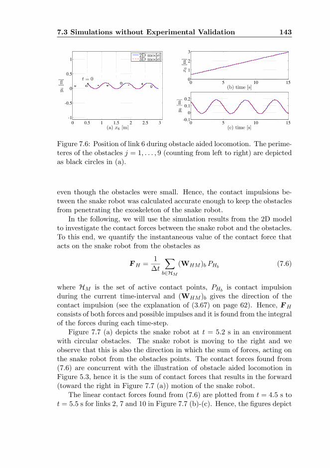
7.3 Simulations without Experimental Validation 143
Figure 7.6: Position of link 6 during obstacle aided locomotion. The perime-teres of the obstacles j = 1; : : : ; 9 (counting from left to right) are depictedas black circles in (a).
even though the obstacles were small. Hence, the contact impulsions be-tween the snake robot was calculated accurate enough to keep the obstaclesfrom penetrating the exoskeleton of the snake robot.
In the following, we will use the simulation results from the 2D modelto investigate the contact forces between the snake robot and the obstacles.To this end, we quantify the instantaneous value of the contact force thatacts on the snake robot from the obstacles as
FH =1
�t
Xb2HM
(WHM )b PHb (7.6)
where HM is the set of active contact points, PHb is contact impulsionduring the current time-interval and (WHM )b gives the direction of thecontact impulsion (see the explanation of (3.67) on page 62). Hence, FH
consists of both forces and possible impulses and it is found from the integralof the forces during each time-step.
Figure 7.7 (a) depicts the snake robot at t = 5:2 s in an environmentwith circular obstacles. The snake robot is moving to the right and weobserve that this is also the direction in which the sum of forces, acting onthe snake robot from the obstacles points. The contact forces found from(7.6) are concurrent with the illustration of obstacle aided locomotion inFigure 5.3, hence it is the sum of contact forces that results in the forward(toward the right in Figure 7.7 (a)) motion of the snake robot.
The linear contact forces found from (7.6) are plotted from t = 4:5 s tot = 5:5 s for links 2, 7 and 10 in Figure 7.7 (b)-(c). Hence, the �gures depict
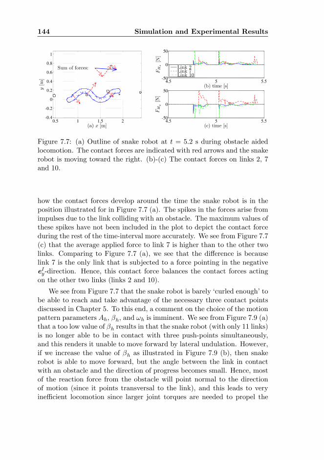
144 Simulation and Experimental Results
Figure 7.7: (a) Outline of snake robot at t = 5:2 s during obstacle aidedlocomotion. The contact forces are indicated with red arrows and the snakerobot is moving toward the right. (b)-(c) The contact forces on links 2, 7and 10.
how the contact forces develop around the time the snake robot is in theposition illustrated for in Figure 7.7 (a). The spikes in the forces arise fromimpulses due to the link colliding with an obstacle. The maximum values ofthese spikes have not been included in the plot to depict the contact forceduring the rest of the time-interval more accurately. We see from Figure 7.7(c) that the average applied force to link 7 is higher than to the other twolinks. Comparing to Figure 7.7 (a), we see that the di¤erence is becauselink 7 is the only link that is subjected to a force pointing in the negativeeIy-direction. Hence, this contact force balances the contact forces actingon the other two links (links 2 and 10).
We see from Figure 7.7 that the snake robot is barely �curled enough�tobe able to reach and take advantage of the necessary three contact pointsdiscussed in Chapter 5. To this end, a comment on the choice of the motionpattern parameters Ah, �h, and !h is imminent. We see from Figure 7.9 (a)that a too low value of �h results in that the snake robot (with only 11 links)is no longer able to be in contact with three push-points simultaneously,and this renders it unable to move forward by lateral undulation. However,if we increase the value of �h as illustrated in Figure 7.9 (b), then snakerobot is able to move forward, but the angle between the link in contactwith an obstacle and the direction of progress becomes small. Hence, mostof the reaction force from the obstacle will point normal to the directionof motion (since it points transversal to the link), and this leads to veryine¢ cient locomotion since larger joint torques are needed to propel the
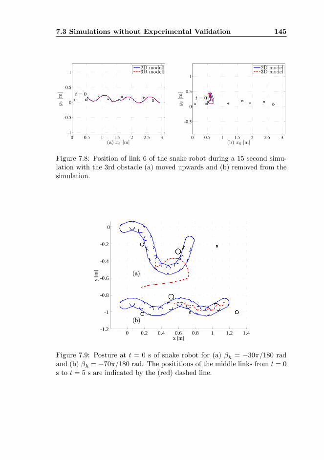
7.3 Simulations without Experimental Validation 145
Figure 7.8: Position of link 6 of the snake robot during a 15 second simu-lation with the 3rd obstacle (a) moved upwards and (b) removed from thesimulation.
0 0.2 0.4 0.6 0.8 1 1.2 1.41.2
1
0.8
0.6
0.4
0.2
0
x [m]
y [m
]
Figure 7.9: Posture at t = 0 s of snake robot for (a) �h = �30�=180 radand (b) �h = �70�=180 rad. The posititions of the middle links from t = 0s to t = 5 s are indicated by the (red) dashed line.
146 Simulation and Experimental Results
snake robot forward (i.e. the contact force needs to be higher to obtainthe same amount of force tangential to the direction of motion with threepush-points). Moreover, the increased contact force will result in that areal snake robot can get easier stuck since the friction forces between theobstacles and the snake robot will increase. The increase in contact forcefor a posture with �more curls�corresponds to the increase in the constraintforces on the wheels for a wheeled snake robot with the same posture duringlateral undulation (without obstacles) as described in Date et al. (2000).The angle between the link in contact with the obstacle and the directionof locomotion will also be smaller if we choose to keep �h at its originalvalue, but lower the amplitude of joint oscillation Ah. Hence, the valueof �h should be chosen such that the snake robot is just �curled enough�to utilize the push-points for locomotion, and the amplitude of oscillationshould, up to some extent, be chosen as high as possible to obtain a largeangle between the direction of locomotion and the links in contact with thepush-points. However, it is important to be aware of that if the obstaclesare located far from each other, a larger value of �h is necessary to allowthe snake robot to reach all three necessary push-points. Moreover, thewave propagation speed is dependent on �h, so this also has to be takeninto account when choosing the motion pattern parameters.
It now remains to comment on the value of the angular frequency !h.For an in�nitely strong snake robot (both with respect to actuator torquesand outer shell) and �xed obstacles that do not yield, a larger !h will resultin a greater forward speed since the propagating wave is propagated fastertoward the back of the snake robot. However, the larger the speed, theharder the impact between the snake robot and the obstacles will become.Also, the speed will be limited by the amount of torque the actuators areable to produce. Moreover, the obstacles may not always be �xed to theground, such as a chair or a small rock, hence it may in some cases benecessary to limit the forces exerted on the obstacle to keep them �xed.This is also achieved by limiting the angular frequency !h. From the dis-cussion above, we choose to keep the motion parameters as they are for theupcoming experiments.
In addition to the perfect scenario depicted in Figure 7.8 (with respectto the connection between the motion pattern and obstacle placement)described above, we set the obstacles according to Table 7.3 and brie�yexplore the scenario where obstacle 3 (counting from the beginning of thetrack) is partly and completely removed. First, obstacle 3 is moved onesnake robot link diameter along the eIy-axis. Thus, its new position in the
7.3 Simulations without Experimental Validation 147
horizontal�eIx; e
Iy
�-plane is
H3;moved : (0:882 m; 0:101 m+ 2LSC1) : (7.7)
Figure 7.8 (a) illustrates the path of link 6 of the snake robot when itmoves through the altered track. The simulation shows that the snakerobot started sliding to the left and rotating anti-clockwise when it wassupposed to collide with the moved obstacle. However, the deviation fromits original path was not substantial enough to hinder the snake robot inreaching obstacle 4 su¢ ciently accurate to continue its path along the track.Secondly, obstacle 3 is completely removed and the new path of the snakerobot is depicted in Figure 7.8 (b). Then the snake robot also rotated anti-clockwise and slid to the left when it was supposed to hit obstacle 3, butthis time it was unable to complete the track since it never collided with thethird obstacle, and therefore never regained the third contact point neededfor locomotion as discussed in Section 5.5.
We might expect that the snake robot fails to move through the entiretrack with one obstacle moved or missing since the desired joint patternis preprogrammed. However, the results displayed in Figure 7.8 show thatsome repositioning of the obstacles is possible. Hence, a control algorithmfor intelligent obstacle aided locomotion does not need to provide a motionpattern fully accurate compared to the position of the obstacles. The snakerobot still manages to move through the track even if it touches someobstacles in a far from perfect manner. The downside can be that largerjoint torques are needed as discussed in Section 5.3.
7.3.5 Robot Model: Comparison of Controllers
The input-output linearizing controller presented in Chapter 6 will be com-pared to a PD-controller in this section. The comparison will be performedfor the (planar) process plant model, or �robot model�, presented in thesame chapter for both a smooth approximation to Coulomb friction, andCoulomb friction described by a set-valued force law. In addition, we willsee how the controllers perform when noise is introduced in the system andthe suitability of the �robot model�for numerical treatment is discussed.
Particular simulation parameters: None. All parameters are given inTables 7.1 and 7.2. Note that (�Cx ; �Cy) and (�Vx ; �Vy) are employedin the robot model instead of (�Tx ; �Ty) since we here have viscousfriction in addition to Coulomb friction.
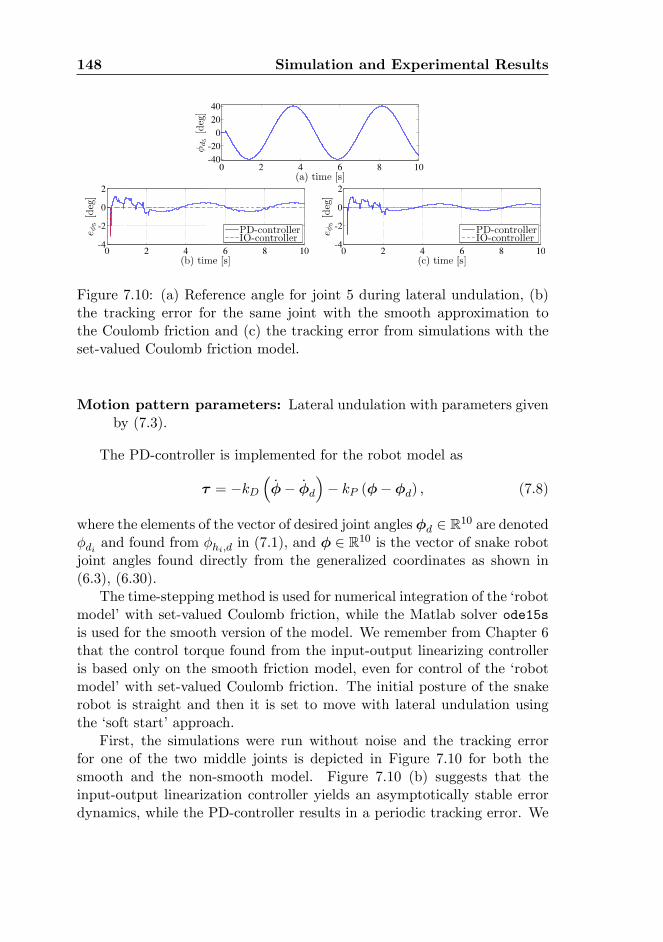
148 Simulation and Experimental Results
Figure 7.10: (a) Reference angle for joint 5 during lateral undulation, (b)the tracking error for the same joint with the smooth approximation tothe Coulomb friction and (c) the tracking error from simulations with theset-valued Coulomb friction model.
Motion pattern parameters: Lateral undulation with parameters givenby (7.3).
The PD-controller is implemented for the robot model as
� = �kD�_�� _�d
�� kP (�� �d) ; (7.8)
where the elements of the vector of desired joint angles �d 2 R10 are denoted�di and found from �hi;d in (7.1), and � 2 R
10 is the vector of snake robotjoint angles found directly from the generalized coordinates as shown in(6.3), (6.30).
The time-stepping method is used for numerical integration of the �robotmodel�with set-valued Coulomb friction, while the Matlab solver ode15sis used for the smooth version of the model. We remember from Chapter 6that the control torque found from the input-output linearizing controlleris based only on the smooth friction model, even for control of the �robotmodel�with set-valued Coulomb friction. The initial posture of the snakerobot is straight and then it is set to move with lateral undulation usingthe �soft start�approach.
First, the simulations were run without noise and the tracking errorfor one of the two middle joints is depicted in Figure 7.10 for both thesmooth and the non-smooth model. Figure 7.10 (b) suggests that theinput-output linearization controller yields an asymptotically stable errordynamics, while the PD-controller results in a periodic tracking error. We
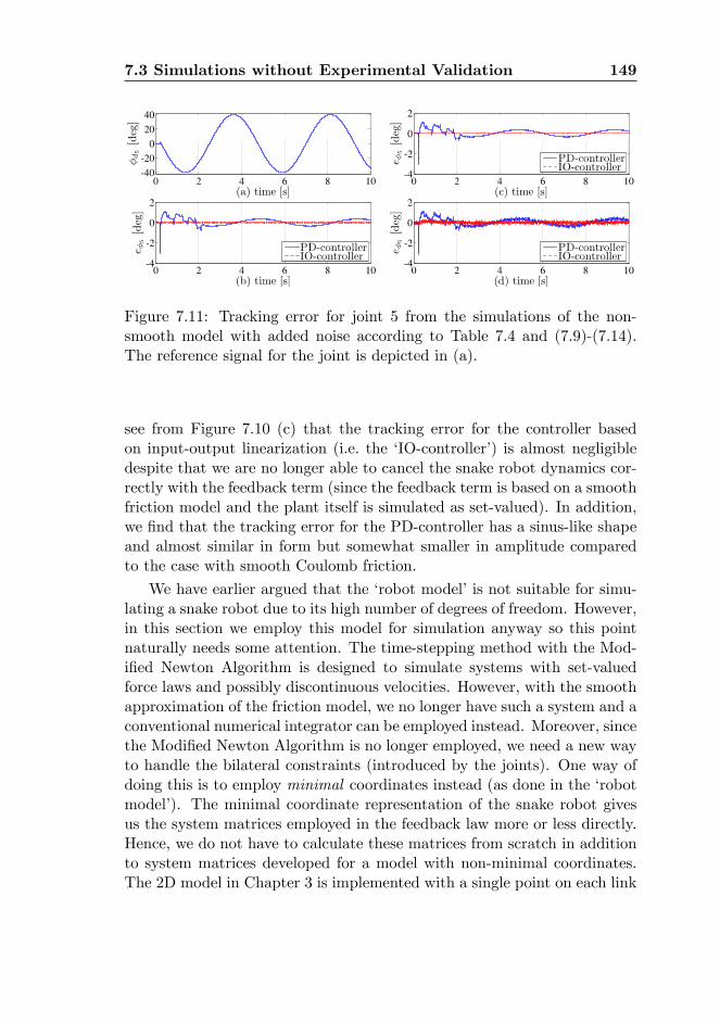
7.3 Simulations without Experimental Validation 149
Figure 7.11: Tracking error for joint 5 from the simulations of the non-smooth model with added noise according to Table 7.4 and (7.9)-(7.14).The reference signal for the joint is depicted in (a).
see from Figure 7.10 (c) that the tracking error for the controller basedon input-output linearization (i.e. the �IO-controller�) is almost negligibledespite that we are no longer able to cancel the snake robot dynamics cor-rectly with the feedback term (since the feedback term is based on a smoothfriction model and the plant itself is simulated as set-valued). In addition,we �nd that the tracking error for the PD-controller has a sinus-like shapeand almost similar in form but somewhat smaller in amplitude comparedto the case with smooth Coulomb friction.
We have earlier argued that the �robot model�is not suitable for simu-lating a snake robot due to its high number of degrees of freedom. However,in this section we employ this model for simulation anyway so this pointnaturally needs some attention. The time-stepping method with the Mod-i�ed Newton Algorithm is designed to simulate systems with set-valuedforce laws and possibly discontinuous velocities. However, with the smoothapproximation of the friction model, we no longer have such a system and aconventional numerical integrator can be employed instead. Moreover, sincethe Modi�ed Newton Algorithm is no longer employed, we need a new wayto handle the bilateral constraints (introduced by the joints). One way ofdoing this is to employ minimal coordinates instead (as done in the �robotmodel�). The minimal coordinate representation of the snake robot givesus the system matrices employed in the feedback law more or less directly.Hence, we do not have to calculate these matrices from scratch in additionto system matrices developed for a model with non-minimal coordinates.The 2D model in Chapter 3 is implemented with a single point on each link
150 Simulation and Experimental Results
for the frictional contact between the snake robot and the ground surface.This choice has been made to simplify the model. Hence, such an approachresults in that a purely rotational motion of a link does not give rise toany friction forces. Such friction forces are needed in the stability analysisprovided of the closed-loop system with the input-output linearizing con-troller. Due to the reasons mentioned above, we decided to try to use thesmooth �robot model�for simulation in order to compare the PD-controllerand the input-output linearizing controller. We see from Figure 7.10 thatwe were able to simulate the system with this approach, and to avoid hav-ing to redesign the 2D model to add a friction point and viscous friction,we also used the same approach (now with the time-stepping method) forthe �robot model�with set-valued friction. Using this approach was okay,but only since we needed a very limited number of simulation trials. This isbecause the simulations were very time-consuming. This was partly due tothe sti¤ di¤erential equations which was due to the smooth approximationof the Coulomb friction, but also due to the enormous amount of terms thathad to be calculated in order to �nd the system matrices. To illustrate thedi¤erence in computation time, we mention that it took between 20 and 50minutes to simulate a single second of snake robot motion with the �robotmodel�, and with the 2D model it only took about 0.5 minutes to simulatea second of snake robot motion.
For the second set of simulations, we add various degrees of noise tothe measurements and test the IO-controller and the PD-controller in sim-ulations where the set-valued Coulomb friction model is employed. Thenoise is added to the measurements with the Matlab function rand whichproduces approximately normally distributed numbers between 0 and 1.Furthermore, the states utilized in the feedback (i.e. the measurementswith noise) are found from
IrO2;m = IrO2 +Np (2 rand (2; 1)� 1) ; (7.9)
�m = � +N� (2 rand (1; 1)� 1) ; (7.10)
�m = �+N� (2 rand (10; 1)� 1) ; (7.11)
IvO2;m = IvO2 +Nv (2 rand (2; 1)� 1) ; (7.12)_�m = _� +N _� (2 rand (1; 1)� 1) ; (7.13)_�m = _�+N _� (2 rand (10; 1)� 1) ; (7.14)
whereNp, N�, N�, Nv, N _� andN _� are positive constants in R, and rand (a; b)is the Matlab function rand that returns a matrix (or vector) with a rowsand b columns with approximately normally distributed numbers between0 and 1.
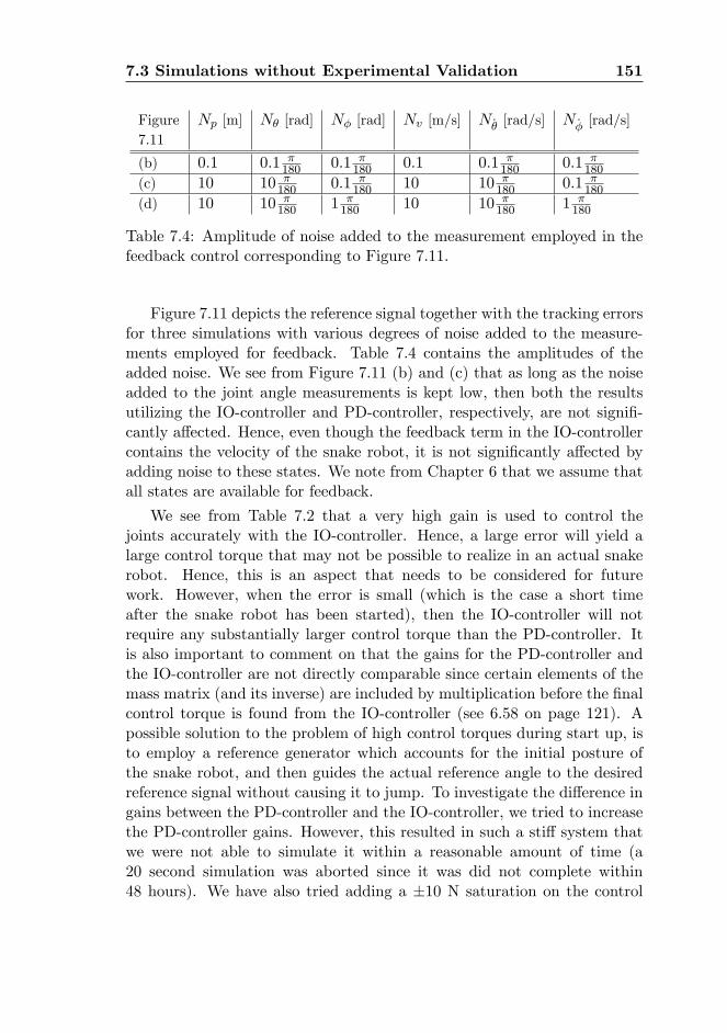
7.3 Simulations without Experimental Validation 151
Figure7.11
Np [m] N� [rad] N� [rad] Nv [m/s] N _� [rad/s] N _� [rad/s]
(b) 0:1 0:1 �180 0:1 �
180 0:1 0:1 �180 0:1 �
180
(c) 10 10 �180 0:1 �
180 10 10 �180 0:1 �
180
(d) 10 10 �180 1 �
180 10 10 �180 1 �
180
Table 7.4: Amplitude of noise added to the measurement employed in thefeedback control corresponding to Figure 7.11.
Figure 7.11 depicts the reference signal together with the tracking errorsfor three simulations with various degrees of noise added to the measure-ments employed for feedback. Table 7.4 contains the amplitudes of theadded noise. We see from Figure 7.11 (b) and (c) that as long as the noiseadded to the joint angle measurements is kept low, then both the resultsutilizing the IO-controller and PD-controller, respectively, are not signi�-cantly a¤ected. Hence, even though the feedback term in the IO-controllercontains the velocity of the snake robot, it is not signi�cantly a¤ected byadding noise to these states. We note from Chapter 6 that we assume thatall states are available for feedback.
We see from Table 7.2 that a very high gain is used to control thejoints accurately with the IO-controller. Hence, a large error will yield alarge control torque that may not be possible to realize in an actual snakerobot. Hence, this is an aspect that needs to be considered for futurework. However, when the error is small (which is the case a short timeafter the snake robot has been started), then the IO-controller will notrequire any substantially larger control torque than the PD-controller. Itis also important to comment on that the gains for the PD-controller andthe IO-controller are not directly comparable since certain elements of themass matrix (and its inverse) are included by multiplication before the �nalcontrol torque is found from the IO-controller (see 6.58 on page 121). Apossible solution to the problem of high control torques during start up, isto employ a reference generator which accounts for the initial posture ofthe snake robot, and then guides the actual reference angle to the desiredreference signal without causing it to jump. To investigate the di¤erence ingains between the PD-controller and the IO-controller, we tried to increasethe PD-controller gains. However, this resulted in such a sti¤ system thatwe were not able to simulate it within a reasonable amount of time (a20 second simulation was aborted since it was did not complete within48 hours). We have also tried adding a �10 N saturation on the control
152 Simulation and Experimental Results
torques for both controllers. Then, the results from stationary motion werethe same as Figure 7.10. However, the steps in the reference signal duringthe �soft start�approach caused a very short, but larger tracking error forthe IO-controller compared to the PD-controller.
The smooth approximation of the Coulomb friction in the �robot model�results in a sti¤ system. This is not advantageous for simulation and the2D model in Chapter 3 should be employed instead. However, since thenon-linear control techniques employed in this thesis are only �t to copewith smooth non-linear systems, the smooth approximation is necessaryfor the controller synthesis and stability proof. Hence, the system matricesfor the minimal coordinates needed to be found in order to implement thecontrol law (which is constructed from these matrices). Thus, even thoughthe simulation time became much longer due to the need for small time stepdue to e.g. the sti¤ system equations, it was more e¤ective to simulate therobot model since few simulations were required to compare the controllers.
7.4 Experimental Setup
The snake robot �Aiko�is employed in the experiments, and the snake robottogether with the rest of the equipment used to conduct the experimentaltests are described in the following.
Each 2 DOF cardan joint of the snake robot is actuated by two 6 WDC-motors. Each the two joint angles are controlled by simple P-controllersimplemented on an Atmel ATmega128 microcontroller. Hence, 10 micro-controllers are employed to control the 10 cardan joints. The snake robotjoint reference angles are sent with a frequency of 10 Hz from a PC runningMatlab, via a CAN-bus (a particular type of �eld bus) to the microcon-trollers. The position of the centre of the middle link (link 6) is trackedusing a Vicon MX Motion Capture System with 4 cameras (MX3) togetherwith Matlab Simulink. The Vicon programme (Vicon iQ 2.0) runs on acomputer with 4 Intel Xeon 3 GHz processors and 2 GB RAM. This wasthe same computer employed for the simulations. The logging of motiondata is synchronized in time through a TCP-connection between the PCthat controls Aiko and the Vicon-computer at the start-up of the transmis-sion of the desired snake robot joint angles. Data logging is performed at20 Hz. We have chosen to let the position of link 6 represent the positionof the snake robot, because then we �lter any transient behaviour of thesnake robot that might occur at its ends and it is thus easier to focus onthe general motion of the snake robot.
7.5 Simulations with Experimental Validation 153
The snake robot moves on particle boards in the experiments. Forobstacle aided locomotion, we attach obstacles cut from a PVC-pipe with0.25 m outer diameter to the particle boards.
7.5 Simulations with Experimental Validation
In this section we compare the simulation and experimental results forsidewinding, lateral undulation with isotropic friction and obstacle aidedlocomotion. We compare both qualitative and quantitative motion to seeto what degree the models can reproduce the motion of the snake robot�Aiko�. Moreover, by investigating obstacle aided locomotion, we can learnwhether the exoskeleton de�ned for the snake robot models resembles theactual contact between Aiko and the obstacles in the experimental setup.We employ the PD-controllers described in Chapters 3 and 4 for the 2D and3D models, respectively. The experimental setup described in Section 7.4has been employed to conduct and log the experiments.
7.5.1 3D Model: Sidewinding
In this section we compare the simulation results with the 3D model andthe experimental results with Aiko for the sidewinding motion pattern.
Particular simulation parameters: None.
Motion pattern parameters: Sidewinding with the same parameters asin (7.5).
The resulting motion of sidewinding with isotropic friction for the 3Dmodel of the snake robot is compared to experimental results found byletting Aiko move with the same motion pattern. We employ the motionpattern parameters given by (7.5) and calculate the reference angles for thejoints from (7.1)-(7.2) with the �soft start�approach starting from a straightand �at posture along the eIx-axis as performed in the sidewinding simula-tions above. The motion of the model and Aiko is depicted in Figure 7.12.As seen from the picture, Aiko was not wearing its metal head. The headwas removed in order to obtain a uniform weight distribution along thesnake robot.
Figure 7.13 displays the position of link 6 for the 3D model and Aiko dur-ing sidewinding. We observe from the �gure that the model almost followsthe eIy-axis, while Aiko steadily turns somewhat to the right. In addition,
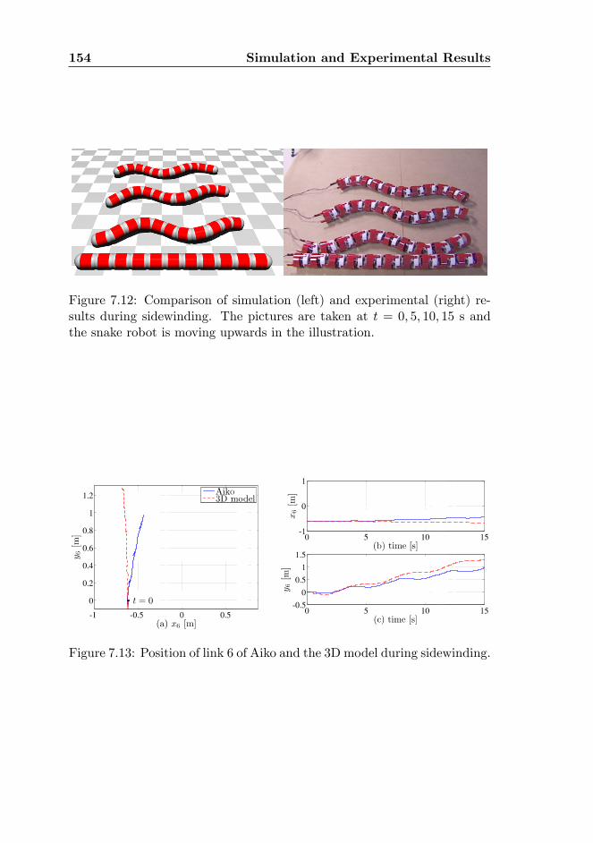
154 Simulation and Experimental Results
Figure 7.12: Comparison of simulation (left) and experimental (right) re-sults during sidewinding. The pictures are taken at t = 0; 5; 10; 15 s andthe snake robot is moving upwards in the illustration.
Figure 7.13: Position of link 6 of Aiko and the 3D model during sidewinding.
7.5 Simulations with Experimental Validation 155
the model covers a greater distance than Aiko. We see from Figure 7.13 (a)and (c) that the simulation results have the same trend and approximatefrequency as the experimental results along the eIy-axis. The variance intrend is more noticeable along the eIx-axis due to the turning motion ofAiko. Moreover, a slight initial di¤erence between the orientation of Aikoand the model may contribute to the discrepancy in heading. We discussin Section 7.5.4 various reasons for the di¤erences between the simulationand experimental results. For sidewinding, we believe that one of the mostimportant di¤erences between the 3D model and Aiko is that Aiko is notable to control its joints accurately (see Section 7.5.4). This is particularlythe case for vertical (lifting) motion which is needed for sidewinding. Byinspecting Aiko closely during the experiment, we noticed that a large partof its body was touching the ground at the same time. This was not thecase in the simulation where the snake robot joints were accurately con-trolled which resulted in that most if its body was lifted from the groundduring locomotion.
We observe from Figure 7.13 (a) and (c) that Aiko sometimes slidesa little backward (at t � 5 s, t � 9 s and t � 14 s). We have tried toreproduce this phenomenon in the 3D model by lowering and increasingthe friction coe¢ cient. We have also tried a variety of anisotropic frictionproperties, but without any luck. The backward motion might be a resultof Aiko not being able to lift its links properly. The links that are supposedto be lifted and moved forward are instead sometimes dragged along theparticle board. This results in a friction force which acts in the oppositedirection of the desired motion of the snake robot. This friction force mightresult in that some of the parts that are supposed to be lying stationary onthe ground are instead pushed slightly backward.
7.5.2 2D and 3D Model: Lateral Undulation with IsotropicFriction
Although not commonly used, it is possible for a snake robot to use lateralundulation for locomotion when the friction between the ground and thesnake robot is isotropic (Nilsson, 2004). In this section we compare thesimulation results from the 2D and 3D model with experimental results ofAiko moving by lateral undulation.
Particular simulation parameters: None.
Motion pattern parameters: Lateral undulation with motion patternparameters given by (7.3).
156 Simulation and Experimental Results
We let the snake robot start in a curved posture with its centre lineapproximately along the eIx-axis and with its initial joints angles given by�hi;d (0) and �vi;d (0) (the latter only applies for the 3D model). Figure 7.14shows both the position of link 6 calculated from the mathematical modelsin the simulations and the position logged from the experiment with Aiko.We see that the snake robot moves slowly backward along the eIx-axis inboth the simulations and the experiment. The average speed of the link isapproximately �1 cm/s. From Figure 7.14, we see that the both the 2Dand the 3D model display the same trend in motion as observed in the ex-periment. However, the distance travelled is greater in the simulations andwe have tried varying the friction coe¢ cients (while still keeping isotropicfriction), but this did not seem to have a noticeable e¤ect on the simulationresults. The di¤erence in distance travelled may come as a consequence ofthat the model of the snake robot is able to control its joints more accu-rately and thus is able to reach the maximum amplitude (40 degrees) whenit is required to do so. Also, this suggest that the frictional contact be-tween the snake robot and the ground surface is more complex than whathas been accounted for in the 2D and 3D model. This statement is alsobacked up by the fact that the simulation results di¤ers between the 2Dand the 3D model. The di¤erences between the two simulations come fromthat two contact points are employed for contact between a link and theground surface in the 3D model, while only a single point is employed forcontact in the 2D model. We have de�ned two contact points in the 3Dmodel to avoid that parts of a link penetrates the ground surface while stillkeeping the contact model as simple as possible (if just a single point wouldhave been chosen for the contact point, then the remaining parts of the linkcan penetrate the ground surface during 3D motion).
In the following section we will see how the snake robot moves with theexact same motion pattern in an environment with obstacles. To comparethe two trials, we have kept the metal sphere head on Aiko for the lateralundulation on an isotropic surface as shown in this section.
7.5.3 2D and 3D Model: Obstacle Aided Locomotion
The simulation and experimental results for obstacle aided locomotion willbe compared in this section. By doing this we can check whether themodels are appropriate test beds for such locomotion, and we can also getan indication of whether the de�nition of the exoskeleton of the models isvalid for describing Aiko.
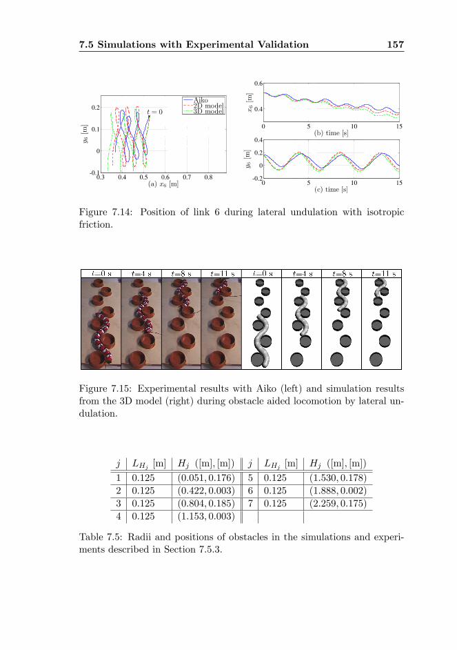
7.5 Simulations with Experimental Validation 157
Figure 7.14: Position of link 6 during lateral undulation with isotropicfriction.
Figure 7.15: Experimental results with Aiko (left) and simulation resultsfrom the 3D model (right) during obstacle aided locomotion by lateral un-dulation.
j LHj [m] Hj ([m]; [m]) j LHj [m] Hj ([m]; [m])
1 0:125 (0:051; 0:176) 5 0:125 (1:530; 0:178)
2 0:125 (0:422; 0:003) 6 0:125 (1:888; 0:002)
3 0:125 (0:804; 0:185) 7 0:125 (2:259; 0:175)
4 0:125 (1:153; 0:003)
Table 7.5: Radii and positions of obstacles in the simulations and experi-ments described in Section 7.5.3.
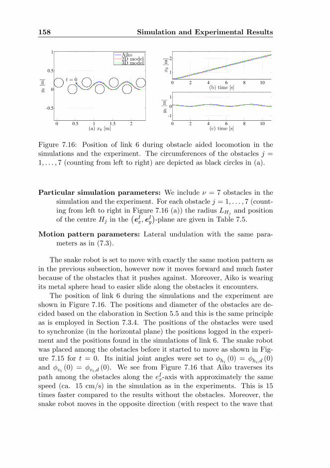
158 Simulation and Experimental Results
Figure 7.16: Position of link 6 during obstacle aided locomotion in thesimulations and the experiment. The circumferences of the obstacles j =1; : : : ; 7 (counting from left to right) are depicted as black circles in (a).
Particular simulation parameters: We include � = 7 obstacles in thesimulation and the experiment. For each obstacle j = 1; : : : ; 7 (count-ing from left to right in Figure 7.16 (a)) the radius LHj and positionof the centre Hj in the
�eIx; e
Iy
�-plane are given in Table 7.5.
Motion pattern parameters: Lateral undulation with the same para-meters as in (7.3).
The snake robot is set to move with exactly the same motion pattern asin the previous subsection, however now it moves forward and much fasterbecause of the obstacles that it pushes against. Moreover, Aiko is wearingits metal sphere head to easier slide along the obstacles it encounters.
The position of link 6 during the simulations and the experiment areshown in Figure 7.16. The positions and diameter of the obstacles are de-cided based on the elaboration in Section 5.5 and this is the same principleas is employed in Section 7.3.4. The positions of the obstacles were usedto synchronize (in the horizontal plane) the positions logged in the experi-ment and the positions found in the simulations of link 6. The snake robotwas placed among the obstacles before it started to move as shown in Fig-ure 7.15 for t = 0. Its initial joint angles were set to �hi (0) = �hi;d (0)and �vi (0) = �vi;d (0). We see from Figure 7.16 that Aiko traverses itspath among the obstacles along the eIx-axis with approximately the samespeed (ca. 15 cm/s) in the simulation as in the experiments. This is 15times faster compared to the results without the obstacles. Moreover, thesnake robot moves in the opposite direction (with respect to the wave that
7.5 Simulations with Experimental Validation 159
is propagated down its body) of what it did for isotropic friction withoutobstacles. Hence, for isotropic friction without obstacles, the direction ofmotion is the same as the direction the undulating wave that is propagatedalong the snake robot body. However, for anisotropic friction or with ob-stacles to push against the direction of motion is opposite to the directionof the propagating wave. Another way of increasing the velocity of a snakerobot on a �at surface is to attach passive caster wheels on the undersideof the robot. However, this approach has some downsides. First of all thesnake robot is more dependent on the ground surface condition for e¤ectivelocomotion. Secondly, the speed of the snake robot is dependent on the an-gular frequency of oscillation !h in (7.1) for a �xed �h and Ah (Saito et al.,2002), and for a snake robot with passive wheels, the side-ways slip has tobe considered when setting !h (Wiriyacharoensunthorn and Laowattana,2002). However, the only practical limitation for the wave propagationspeed during obstacle aided locomotion with obstacles that do not yield(i.e. move or deform when pushed against) is the speed of the joint mo-tors. It is therefore possible to gain great velocities using obstacle aidedlocomotion.
7.5.4 Discussion of the Experimental Validation
We have seen in the previous section (Section 7.4) that the simulationand experimental results range from being very similar, as for the obstacleaided locomotion in Figure 7.16, to comparing fairly well for sidewindingin Figure 7.13. Consequently, the di¤erences between the results need tobe addressed and in the following we will list the most important possiblesources for the discrepancies:
� Aiko has a noticeable free play in the joints of about 3 � 5 degrees.This results in that the control of the joint angles is not completelyaccurate and the joint angle might not be able to reach its desiredangle.
� The dynamics of the actuators are not modelled. Hence, the actu-ators in the models are extremely strong and fast, and we are ableto accurately control the actual angle of each joint to its desired po-sition. This is not the case for Aiko where the joint motors some-times saturate and are unable to track the desired joint movementprecisely. This particularly the case for vertical motion where largerjoint torques are required.
160 Simulation and Experimental Results
� For each cardan joint, there is in fact a 2.2 cm distance between therotational axis for the yaw and pitch motion. However, to simplifythe kinematics in the models, we have assumed that the axes crosseach other.
� The varnish on the underside of the snake robot has been worn down.This has resulted in that the snake robot links slide easier when rolledslightly to one of the sides where the varnish is still present.
� The Stribeck e¤ect (see e.g. Leine and Nijmeijer (2004)) is not in-cluded in the model of the friction. The Stribeck e¤ect states, roughlyspeaking, that the friction forces acting on a body is reduced just afterit is set in motion.
� The exoskeleton of Aiko is not modelled precisely since this wouldrequire a great deal of consideration of the geometry of the snake robotand this would severely complicate the expressions for the contactwith the environment.
� There was a time-delay between the start-up of the snake robot andthe start-up of the logging of position data. This delay ranged be-tween 50 and 150 ms.
� We note from the simulations with lateral undulation with isotropicfriction that there is a di¤erence between the simulation results ofthe 2D and the 3D model. The di¤erence may arise from the factthat two friction points are employed for each link in the 3D modelto handle the impacts with the ground in an e¤ective manner, whilethe 2D model only has one friction point per link to minimize thecomplexity of the model and thus increase the simulation speed.
Even though there are several sources of error, we see from the plotsthat compare the simulation and experimental results that the models givea satisfactory qualitative description of the snake robot dynamics. Espe-cially the direction of locomotion is fairly accurate. For the sidewindingmotion pattern, the model is not accurate enough to predict the quantita-tive motion of the snake robot for an extended period of time, however itgives a clear indication of how the snake robot will move. This suggeststhat the model can be used to develop and test new 3D motion patterns forsnake robots that can later be implemented on physical snake robots suchas Aiko.
7.6 Summary 161
7.6 Summary
In this chapter we present back-to-back comparisons between simulationand experimental results for a selection of serpentine motion patterns. Fur-thermore, additional simulation results are given to test motion patternsand controllers which we have not been able to investigate in the experi-mental setup with our snake robot Aiko.
We see from the simulations that the time-stepping method with theModi�ed Newton Euler Algorithm is suitable for numerical treatment ofthe 2D and 3D model. This is veri�ed, partly by simulating that the snakerobot drops to the ground and then moves forward by lateral undulation.For this scenario the numerical treatment is stable even though the contactforces are large and many impacts occurs.
The 3D model gives realistic simulation results of both sidewinding andU-shaped lateral rolling. To this end, the snake robot moves sideways bylateral rolling due to our choice of an exoskeleton for contact with theground surface. Also, our choice of possible contact points between thesnake robot and the ground surface keeps all parts of the snake robot linksfrom penetrating the ground surface. Sidewinding and U-shaped lateralrolling are tested for a selection of anisotropic friction properties, and wehave found that the friction coe¢ cients in�uence the direction of motionfor these motion patterns.
The 2D and 3D model are both simulated for obstacle aided locomotionwith small obstacles. Even though the obstacles are small, the snake robotdoes not get stuck since we de�ne the contact between the snake robot andan obstacle as a moving contact point. This results in that every point onthe body of the snake robot can come in contact with the obstacle andthe obstacle is kept from penetrating the exoskeleton of the snake robot.We see that the simulation results compare very well for obstacle aidedlocomotion simulated with the 2D and the 3D model. For lateral undulationwith isotropic friction (without obstacles), there is a noticeable di¤erencebetween the models. However, both models move in the same direction(backward) and the qualitative motion of the snake robot is the same.
By comparing Figure 7.3 with Figure 7.16, we note that the snake robotis able to move much faster by pushing against obstacles than while movingon a planar surface with 2.5 times higher friction coe¢ cient transversal tothe snake robot than along it. To obtain the same speed on a planar surfacewithout obstacles, the snake robot would probably have to be equipped withwheels which complicates its design. It addition, the use of obstacles rendersthe snake robot less dependent on the condition of the ground surface. This
162 Simulation and Experimental Results
is a desirable mobility property.The simulations given in Section 7.3.5 show that the input-output lin-
earizing controller proposed in Chapter 6 performs better that a conven-tional PD-controller for the controller gains used in that section, even whennoise up to a certain level is introduced in the measurements. However,there is an issue with the choice of controller gains since it was not possibleto simulate very high gains for the PD-controller due to the resulting sti¤model. However, for stationary motion, the IO-controller performed betterthan the PD-controller even though the applied torques were almost thesame in magnitude.
From the back-to-back comparisons between simulation and experimen-tal results, we conclude that the 2D and 3D model both give a realisticpicture of how a real snake robot will move, especially for obstacle aidedlocomotion. Many aspects of Aiko have not been included in the mathemat-ical model, which results in noticeable di¤erences between the simulationand experimental results. However, the goal of the modelling is not to ex-actly reproduce the behaviour of the speci�c snake robot Aiko. To achievesuch an exact similarity, more elaborate system identi�cation has to beperformed and the exterior of the snake robot has to be more accuratelymodelled. Instead of presenting a model with such a very close resem-blance to Aiko, we present models for synthesis and testing of planar and3D motion patterns for snake robots in general.
In this chapter we employ three mathematical models: the 2D modelfrom Chapter 3, the 3D model from Chapter 4 and the �robot model�pre-sented in Chapter 6. Each model is developed for its own speci�c purpose.First, the 2D model is developed to have an as simple model as possiblefor fast implementation and simulation of planar motion pattern. Second,the 3D model is for synthesis and testing of a combination of planar and3D motion patterns. Third, the �robot model�is developed to implementand investigate stability of state-feedback controllers. However, it is notadvantageous to use for simulation, partly since it takes approximately 20to 50 times more time to simulate the planar �robot model�than it takes tosimulate the 2D model. We see in this chapter that the roles of the di¤erentmodels are successfully ful�lled.
Chapter 8
Conclusions and FurtherWork
The results presented in this thesis are steps towards developing snakerobots that can navigate e¢ ciently in narrow and chaotic environments, forexample, when searching for people in a collapsed building or inspectingnarrow and possibly dangerous areas of industrial plants. In addition, theresults can be used to better understand the working principle of biologicalsnake locomotion.
A novel 2D mathematical model based on the framework of non-smoothdynamics and convex analysis is developed for a snake robot in a certainenvironment with external objects. The model describes planar snake robotmotion where the snake robot can push against external obstacles over theentire surface of each link. Hence, the e¤ect of the contact forces betweenthe obstacle and each link is modelled properly. It is shown how to easilyincorporate the normal contact and friction forces into the system dynamics(which is represented by a certain equality of measures) by set-valued forcelaws. Moreover, it is shown how to include the correct directional Coulombfriction.
The 2D model is extended to a 3D non-smooth mathematical modelbased on the same methodology. However, for the 3D model we need toadd the ability to lift the links above the ground. Moreover, a 3D surfacehas to be de�ned for each link. Such a surface is used for contact withthe ground surface and obstacles. This allows us to simulate 3D motionpatterns such as sidewinding and lateral rolling. Even though the resultingdynamics is hybrid (there may be velocity jumps due to impacts), there isno need for an explicit switch between system equations (when for example
164 Conclusions and Further Work
an impact between the snake robot and an obstacle occurs) since both thenon-impulsive forces and the impact impulses are covered by the same forcelaw and since we use the time-stepping method for the numerical treatment.The same principles apply for the 2D model. The use of the non-minimalabsolute coordinates results in a constant and diagonal mass matrix and ane¤ective way of writing the system equations. Such a constant mass matrixis bene�cial in the numerical treatment since it needs only to be invertedonce and not for each time-step during simulation.
A control law for tracking control of the joints of a snake robot with-out wheels is proposed. Since the friction between the snake robot andthe ground surface is essential for locomotion for wheel-less snake robots,a kinematic model is not su¢ cient and a non-linear model including boththe kinematics and dynamics of a planar snake robot and its contact withthe ground surface is presented. To this end, we develop a planar modelof the snake robot based on the standard dynamics of a robot manipulatorThis model is denoted the process plant model or �robot model�and it isinitially implemented with a smooth approximation of Coulomb friction.Such a formulation is advantageous for control since it allows us to employthe large variety of control techniques available for robot manipulators.Furthermore, a control plant model is developed from the process plantmodel. This model allows for an in�nite number of rotations of the snakerobot without a¤ecting the controller. Based on this control plant model,a non-linear controller is developed using input-output linearization. It isproved using Lyapunov stability theory that this controller asymptoticallystabilizes the desired motion for the snake robot joints. Furthermore, simu-lations with this controller applied to the process plant model suggest thatthe closed-loop system is able to track the desired joint angles. In addition,the same process plant model is implemented with a set-valued force lawfor describing the Coulomb friction instead of its smooth approximation.The simulations suggest that the proposed controller is also e¤ective forthe snake robot model with set-valued Coulomb friction. Moreover, it tooka very long time to simulate the process plant model compared to the 2Dmodel, and this suggests that it is not suitable for simulation.
Experiments are performed with the snake robot �Aiko� built at theNTNU/SINTEF Advanced Robotics Laboratory and a back-to-back com-parison between simulation and experimental results is presented. Thecomparison illustrate a quantitative similarity between motion of the 2Dand 3D model and the snake robot �Aiko�during obstacle aided locomotion.Moreover, the results show that the model needs to be extended to accu-rately describe in particular 3D motion of Aiko. We are able to make a more
Conclusions and Further Work 165
exact model of Aiko, and thus deal with issues such as actuator dynamicsand a more accurate description of the exoskeleton of Aiko. However, thiswill require a considerable amount of time and e¤ort and such a speci�cmodel is beyond the scope of this thesis. Instead, we have focused on givinga more general description of a snake robot where Aiko has been employedas an inspiration for the design. The simulation results of the 2D and 3Dmodel illustrate that qualitatively the motions of the simulated snake robotand Aiko are the same. Hence, the 2D and 3D models constitute a test bedfor future controller design and motion pattern design.
This thesis provides a framework based on non-smooth dynamics forthe development, analysis and testing of forthcoming motion planning andcontrol approaches to obstacle aided locomotion. Further work on snakerobots is important to eventually develop a snake robot that can navigateby itself through an unknown and cluttered environment. In the follow-ing we list a number of challenges to overcome before such a scenario isrealizable. 1) Develop motion patterns based on the mathematical modeland observations of real snakes that enable a snake robot to detect andexploit obstacles by itself for e¢ cient locomotion. Such a motion patternwill enable a snake robot to move within, for example, a shattered buildingwhile looking for people. 2) Extend the 3D model to include other groundshapes such as stairs. This will be advantageous for the development ofthe motion pattern mentioned in �1)�. 3) Construct a smooth exterior ofthe snake robot. This will enable the snake robot to easily slide beside orover any irregularities on the ground. 4) Construct robust snake robotswith powerful and lightweight joint actuators to be able to continue beingoperational even though some of the joint actuators break down. 5) De-velop a snake robot exterior that can withstand large temperatures during,for example, a �re-�ghting operation, while still keeping the temperaturewithin the snake robot relatively low. 6) Develop control algorithms thatconsider the global positions of all parts of a snake robot. This will helpkeep the snake robot from unintentionally colliding with its environmentduring operations in fragile environments.
A snake robot has limited payload capability, poor power e¢ ciency and ahigh number of degrees of freedom. Nevertheless, the snake robot has thepotential of great traversability and capability of inspecting narrow places. Itcan also be made very robust to dirt and dust by covering the robot completelywith a shell. These properties make the research on snake robots worth-while. Itis hoped that this thesis will help to promote further research on the fascinatingtopic of snake robots.
166 Conclusions and Further Work
Bibliography
Alart, P. and A. Curnier (1991). A mixed formulation for frictional contactproblems prone to Newton like solution methods. Comput. Method. Appl.M. 92, 353�375.
Ayers, J., C. Wilbur and C. Olcott (2000). Lamprey robots. In: Proc. Int.Symp. Aqua Biomechanisms.
Bauchot, R. (1994). Snakes: A Natural History. Sterling Publishing Com-pany.
Bayraktaroglu, Z. Y., A. Kilicarslan, A. Kuzucu, V. Hugel and P. Blazevic(2006). Design and control of biologically inspired wheel-less snake-likerobot. In: Proc. IEEE/RAS-EMBS Int. Conf. Biomedical Robotics andBiomechatronics. pp. 1001�1006.
Bayraktaroglu, Z. Y. and P. Blazevic (2005). Understanding snakelike lo-comotion through a novel push-point approach. J. Dyn. Syst. - Trans.ASME 127(1), 146�152.
Bayraktarouglu, Z. Y., F. Butel, P. Blazevic and V. Pasqui (1999). A geo-metrical approach to the trajectory planning of a snake-like mechanism.In: Proc. IEEE/RSJ Int. Conf. Intelligent Robots and Systems. pp. 1322�1327.
Bloch, A. M., J. Baillieul, P. Crouch and J. Marsden (2003). NonholonomicMechanics and Control. Springer-Verlag.
Bloch, A. M., P. S. Krishnaprasad, J. E. Marsden and R. M. Murray (1995).Nonholonomic mechanical systems with symmetry. Technical report. Cal-ifornia Institute of Technology.
Boyer, F., M. Porez and W. Khalil (2006). Macro-continuous computedtorque algorithm for a three-dimensional eel-like robot. IEEE Trans. Ro-bot. 22(4), 763�775.
168 Bibliography
Brogliato, B. (1999). Nonsmooth Mechanics. 2 ed. Springer. London.
Brovoll, Sverre (2006). Design and implementation of a snake robot actu-ated by dc-motors. Master�s thesis. Norwegian University of Science andTechnology. In Norwegian.
Burdick, J. W., J. Radford and G. S. Chirikjian (1993). A �sidewinding�locomotion gait for hyper-redundant robots. In: Proc. IEEE Int. Conf.Robotics and Automation. pp. 101�106.
Chen, L., Y. Wang, S. Ma and B. Li (2004). Studies on lateral rollinglocomotion of a snake robot. In: Proc. IEEE Int. Conf. Robotics andAutomation. pp. 5070�5074.
Chernousko, F. (2005). Modelling of snake-like locomotion. Appl. Math.Comput. 164(2), 415�434.
Chernousko, F. L. (2000). Snake-like motions of multibody systems over arough plane. In: Proc. 2nd Int. Conf. Control of Oscillations and Chaos.pp. 321�326.
Chirikjian, G. S. (1992). Theory and Applications of Hyper-RedundantRobotic Manipulators. PhD thesis. California Institute of Technology.Pasadena, California.
Chirikjian, G. S. and J. W. Burdick (1991). Kinematics of hyper-redundantrobot locomotion with applications to grasping. In: Proc. IEEE Int.Conf. Robotics and Automation. pp. 720�725.
Chirikjian, G. S. and J. W. Burdick (1993). Design and experiments witha 30 DOF robot. In: Proc. IEEE Int. Conf. Robotics and Automation.Vol. 3. pp. 113�119.
Chirikjian, G. S. and J. W. Burdick (1994a). A hyper-redundant manipu-lator. IEEE Robotics & Automation Magazine 1(4), 22�29.
Chirikjian, G. S. and J. W. Burdick (1994b). A modal approach tohyper-redundant manipulator kinematics. IEEE Trans. Robot. Autom.10(3), 343�354.
Chirikjian, G. S. and J. W. Burdick (1995). The kinematics of hyper-redundant robot locomotion. IEEE Trans. Robot. Autom. 11(6), 781�793.
Bibliography 169
Choset, H. (2007). Snake robots at Carnegie Mellon University.http://www.snakerobot.com/. Online. Accessed 29 September 2007.
Choset, H. and J. Y. Lee (2001). Sensor-based construction of a retract-likestructure for a planar rod robot. IEEE Trans. Robot. Autom. 17(4), 435�449.
Choset, H., J. Luntz, E. Shammas, T. Rached, D. Hull and C. C. Dent(2000). Design and motion planning for serpentine robots. In: Proc.SPIE Smart Structures and Materials: Smart Electronics and MEMS.Vol. 3990. Newport Beach, CA, USA. pp. 148 �155. Serpentine robots;.
Date, H., Y. Hoshi and M. Sampei (2000). Locomotion control of a snake-like robot based on dynamic manipulability. In: Proc. IEEE/RSJ Int.Conf. Intelligent Robots and Systems.
Date, H., Y. Hoshi, M. Sampei and N. Shigeki (2001). Locomotion controlof a snake robot with constraint force attenuation. In: Proc. AmericanControl Conference. pp. 113�118.
Do Carmo, M. P. (1976). Di¤erential Geometry of Curves and Surfaces.Prentice-Hall. Englewood Cli¤s, New Jersey.
Dowling, K. (1999). Limbless locomotion: learning to crawl. In: Proc. IEEEInt. Conf. Robotics and Automation. Vol. 4.
Dowling, K. J. (1997). Limbless Locomotion. Learing to Crawl with a SnakeRobot. PhD thesis. Carnegie Mellon University.
Egeland, O. and J. T. Gravdahl (2002). Modeling and Simulation for Au-tomatic Control. Marine Cybernetics. Trondheim, Norway.
Erkmen, I., A. M. Erkmen, F. Matsuno, R. Chatterjee and T. Kamegawa(2002). Snake robots to the rescue!. IEEE Robotics & Automation Mag-azine 9(3), 17�25.
Fossen, T. I. (2002). Marine Control Systems: Guidance, Navigation andControl of Ships, Rigs and Underwater Vehicles. Marine Cybernetics.Trondheim, Norway.
Glocker, Ch. (2001). Set-Valued Force Laws, Dynamics of Non-Smooth Sys-tems. Vol. 1 of Lecture Notes in Applied Mechanics. Springer-Verlag.Berlin.
170 Bibliography
Glocker, Ch. and C. Studer (2005). Formulation and preparation for numer-ical evaluation of linear complementarity systems in dynamics. MultibodySystem Dynamics 13, 447�463.
Grabec, I. (2002). Control of a creeping snake-like robot. In: Proc. 7th Int.Workshop on Advanced Motion Control. pp. 526�513.
Gray, J. (1946). The mechanism of locomotion in snakes. J. Exp. Biol.23(2), 101�120.
Gu, Y.-L. and Y. Xu (1993). A normal form augmentation approach toadaptive control of space robot systems. In: Proc. IEEE Int. Conf. Ro-botics and Automation. Vol. 2. pp. 731�737.
Henning, W., F. Hickman and H. Choset (1998). Motion planning for ser-pentine robots. In: Proc. ASCE Space and Robotics.
Hirose, S. (1993). Biologically Inspired Robots: Snake-Like Locomotors andManipulators. Oxford University Press. Oxford.
Hirose, S. and A. Morishima (1990). Design and control of a mobil robotwith an articulated body. Int. J. Rob. Res. 9(2), 99�114.
Hirose, S. and M. Mori (2004). Biologically inspired snake-like robots. In:Proc. IEEE Int. Conf. Robotics and Biomimetics. pp. 1�7.
Hirose, S. and Y. Umetani (1976). Kinematic control of active cord mech-anism with tactile sensors. In: Proc. 2nd RoMAnSy Symp. Warsaw.pp. 241�252.
Kamegawa, T., T. Yarnasaki, H. Igarashi and F. Matsuno (2004). Develop-ment of the snake-like rescue robot �Kohga�. In: Proc. IEEE Int. Conf.Robotics and Automation. Vol. 5. pp. 5081�5086.
Kelly, S. D. and R. M. Murray (1995). Geometric phases and robotic loco-motion. J. Robotic Systems 12(6), 417�431.
Khalil, H. K. (2002).Nonlinear Systems. 3rd ed. Prentice Hall. InternationalEdition.
Kolmanovsky, I. and N. H. McClamroch (1995). Developments in nonholo-nomic control problems. IEEE Contr. Syst. Mag. 15(6), 20�36.
Bibliography 171
Krishnaprasad, P. S. and D. P. Tsakiris (1994). G-snakes: Nonholonomickinematic chains on lie groups. In: Proc. 33rd IEEE Conf. Decision andControl. Vol. 3. Lake Buena Vista, FL USA. pp. 2955�2960.
Le Saux, C., R. I. Leine and Ch. Glocker (2005). Dynamics of a rolling diskin the presence of dry friction. Journal of Nonlinear Science 15(1), 27�61.
Leine, R. I. and H. Nijmeijer (2004). Dynamics and Bifurcations of Non-Smooth Mechanical Systems. Vol. 18 of Lecture Notes in Applied andComputational Mechanics. Springer Verlag. Berlin.
Lewis, M. A. and D. M. Zehnpfennig (1994). R7: A snake-like robot for3-D visual inspection. In: Proc. IEEE/RSJ Int. Conf. Intelligent Robotsand Systems. Vol. 2. Munich Germany. pp. 1310�1317.
Liljebäck, P. (2004). Modular snake-robot: Modeling, implementation andcontrol of a modular and pressure based snake-robot. Master�s thesis.Norwegian University of Technology and Science. Trondheim, Norway.In Norwegian.
Liljebäck, P., Ø. Stavdahl and K. Y. Pettersen (2005). Modular pneumaticsnake robot: 3D modelling, implementation and control. In: Proc. 16thIFAC World Congress.
Lu, Y., S. Ma, B. Li and L. Chen (2003). Ground condition sensing of asnake-like robot. In: Proc. IEEE Int. Conf. Robotics, Intelligent Systemsand Signal Processing. Vol. 2. pp. 1075�1080.
Ma, S. (1999). Analysis of snake movement forms for realization of snake-like robots. In: Proc. IEEE Int. Conf. Robotics and Automation. Vol. 4.Detroit, MI USA. pp. 3007�3013.
Ma, S. (2001). Analysis of creeping locomotion of a snake-like robot. Adv.Robotics 15(2), 205�224.
Ma, S. and N. Tadokoro (2006). Analysis of creeping locomotion of a snake-like robot on a slope. Autonomous Robots 20, 15�23.
Ma, S., H. Araya and L. Li (2001a). Development of a creeping snake-robot.In: Proc. IEEE Int. Symp. Computational Intelligence in Robotics andAutomation. pp. 77�82.
172 Bibliography
Ma, S., N. Tadokoro, B. Li and K. Inoue (2003a). Analysis of creeping lo-comotion of a snake robot on a slope. In: Proc. IEEE Int. Conf. Roboticsand Automation. pp. 2073�2078.
Ma, S., W. J. Li and Y. Wang (2001b). A simulator to analyze creepinglocomotion of a snake-like robot. In: Proc. IEEE Int. Conf. Robotics andAutomation. Vol. 4.
Ma, S., Y. Ohmameuda and K. Inoue (2004). Dynamic analysis of 3-dimensional snake robots. In: Proc. IEEE/RSJ Int. Conf. IntelligentRobots and Systems. pp. 767�772.
Ma, S., Y. Ohmameuda, K. Inoue and B. Li (2003b). Control of a 3-dimensional snake-like robot. In: Proc. IEEE Int. Conf. Robotics andAutomation. Vol. 2. Taipei, Taiwan. pp. 2067 �2072.
Masayuki, A., T. Takayama and S. Hirose (2004). Development of �Souryu-III�: connected crawler vehicle for inspection inside narrow and windingspaces. In: Proc. IEEE Int. Conf. Intelligent Robots and Systems. Vol. 1.pp. 52�57.
Mattison, C. (2002). The Encyclopaedia of Snakes. Cassell Paperbacks. Lon-don.
McIsaac, K. A. and J. P. Ostrowski (1999). A geometric approach to an-guilliform locomotion: Modelling of an underwater eel robot. In: Proc.IEEE Int. Conf. Robotics and Automation. Vol. 4. pp. 2843�2848.
McIsaac, K. A. and J. P. Ostrowski (2000). Motion planning for dynamiceel-like robots. In: Proc IEEE Int. Conf. Robotics and Automation.Vol. 2. pp. 1695�1700.
McIsaac, K. A. and J. P. Ostrowski (2003a). A framework for steeringdynamic robotic locomotion systems. Int. J. Robot. Res. 22(2), 83�97.
McIsaac, K. A. and J. P. Ostrowski (2003b). Motion planning for anguilli-form locomotion. IEEE Trans. Robot. Autom. 19(4), 637�625.
Miller, G. (2002). Neurotechnology for Biomimetic Robots. Chap. SnakeRobots for Search and Rescue, pp. 271�284. MIT Press Cambridge, MA,USA. Cambridge/London.
Miller, G. (2007). Dr. Miller�s snake robots. http://www.snakerobots.com/.Online. Accessed 29 September 2007.
Bibliography 173
Moreau, J. J. (1988). Unilateral contact and dry friction in �nite freedomdynamics. In: Non-Smooth Mechanics and Applications (J. J. Moreauand P. D. Panagiotopoulos, Eds.). Vol. 302 of CISM Courses and Lec-tures. pp. 1�82. Springer Verlag. Wien.
Mori, M. and S. Hirose (2002). Three-dimensional serpentine motion andlateral rolling by active cord mechanism ACM-R3. In: Proc. IEEE/RSJInt. Conf. Intelligent Robots and Systems. pp. 829�834.
Murray, R. M., Z. Li and S. S. Sastry (1994). A Mathematical Introductionto Robotic Manipulation. 1st ed. CRC Press. Florida, USA.
Nijmeijer, H. and A. van der Schaft (1990). Nonlinear Dynamical ControlSystems. Springer-Verlag. New York.
Nilsson, M. (1997a). Ripple and roll: Slip-free snake robot locomotion. In:Proc. Mechatronical Computer Systems for Perception and Action. Piza,Italy.
Nilsson, M. (1997b). Snake robot free climbing. In: Proc. IEEE Int. Conf.Robotics and Automation. Vol. 4. pp. 3415�3420.
Nilsson, M. (1998). Snake robot � free climbing. IEEE Contr. Syst. Mag.18(1), 21�26.
Nilsson, M. (2004). Serpentine locomotion on surfaces with uniform friction.In: Proc. IEEE/RSJ Int. Conf. Intelligent Robots and Systems. pp. 1751�1755.
Ohmameuda, Y. and S. Ma (2002). Control of a 3-dimensional snake-likerobot for analysis of sinus-lifting motion. In: Proc. 41st SICE AnnualConference. Vol. 3. pp. 1487�1491.
Ohno, H. and S. Hirose (2001). Design of slim slime robot and its gaitof locomotion. In: Proc. IEEE/RSJ Int. Conf. Intelligent Robots andSystems. Vol. 2. pp. 707�715.
Ostrowski, J. and J. Burdick (1996). Gait kinematics for a serpentine robot.In: Proc. IEEE Int. Conf. Robotics and Automation. Vol. 2. pp. 1294�1299.
Ostrowski, J. and J. Burdick (1998). The geometric mechanics of undula-tory robotic locomotion. Int. J. Robot. Res. 17(7), 683�701.
174 Bibliography
Poi, G., C. Scarabeo and B. Allotta (1998). Traveling wave locomotionhyper-redundant mobile robot. In: Proc. IEEE Int. Conf. Robotics andAutomation. Vol. 1. pp. 418�423.
Prautsch, P. and T. Mita (1999). Control and analysis of the gait of snakerobots. In: Proc. IEEE Int. Conf. Control Applications. Kohala Coast,HI USA. pp. 502�507.
Rincon, D. M. and J. Sotelo (2003). Ver-Vite: Dynamic and experimentalanalysis for inchwormlike biomimetic robots. IEEE Robot. Autom. Mag.10(4), 53�57.
Rockafellar, R. T. (1970). Convex Analysis. Princeton Landmarks in Math-ematics. Princeton University Press. Princeton, New Jersey.
Saito, M., M. Fukaya and T. Iwasaki (2002). Serpentine locomotion withrobotic snakes. IEEE Contr. Syst. Mag. 22(1), 64�81.
Shan, Y. and Y. Koren (1993). Design and motion planning of a mechanicalsnake. IEEE Trans. Syst. Man Cyb. 23(4), 1091�1100.
Spong, M. W. (1996). Energy based control of a class of underactuated me-chanical systems. In: Proc. 13th IFAC World Congress. Vol. F. pp. 431�436.
Spong, M. W. and M. Vidyasagar (1989). Robot Dynamics and Control.Wiley & Sons Inc.
Tanev, I., T. Ray and A. Buller (2005). Automated evolutionary design, ro-bustness, and adaptation of sidewinding locomotion of a simulated snake-like robot. IEEE Trans. Robot. 21(4), 632�645.
Togawa, K., M. Mori and S. Hirose (2000). Study on three-dimensionalactive cord mechanism: Development of ACM-R2. In: Proc. IEEE/RSJInt. Conf. Intelligent Robots and Systems. Vol. 3. pp. 2242�2247.
Transeth, A. A. and K. Y. Pettersen (2006). Developments in snake robotmodeling and locomotion. In: Proc. IEEE Int. Conf. Control, Automa-tion, Robotics and Vision. Singapore. pp. 1393�1400.
Transeth, A. A. and K. Y. Pettersen (2008). A survey on snake robot mod-eling and locomotion. Robotica. Submitted.
Bibliography 175
Transeth, A. A., N. van de Wouw, A. Pavlov, J. P. Hespanha and K. Y.Pettersen (2007a). Tracking control for snake robot joints. In: Proc.IEEE/RSJ Int. Conf. Intelligent Robots and Systems. San Diego, CA,USA. pp. 3539�3546.
Transeth, A. A., P. Liljebäck and K. Y. Pettersen (2007b). Snake robotobstacle aided locomotion: An experimental validation of a non-smoothmodeling approach. In: Proc. IEEE/RSJ Int. Conf. Intelligent Robotsand Systems. San Diego, CA, USA. pp. 2582�2589.
Transeth, A. A., R. I. Leine, Ch. Glocker and K. Y. Pettersen (2006a). Non-smooth 3D modeling of a snake robot with external obstacles. In: Proc.IEEE Int. Conf. Robotics and Biomimetics. Kunming, China. pp. 1189�1196.
Transeth, A. A., R. I. Leine, Ch. Glocker and K. Y. Pettersen (2006b).Non-smooth 3D modeling of a snake robot with frictional unilateral con-straints. In: Proc. IEEE Int. Conf. Robotics and Biomimetics. Kunming,China. pp. 1181�1188.
Transeth, A. A., R. I. Leine, Ch. Glocker and K. Y. Pettersen (2008a).3D snake robot motion: Non-smooth modeling, simulations, and experi-ments. IEEE Trans. Robot. Accepted.
Transeth, A. A., R. I. Leine, Ch. Glocker, K. Y. Pettersen and P. Liljebäck(2008b). Snake robot obstacle aided locomotion: Modeling, simulations,and experiments. IEEE Trans. Robot. Accepted.
Wiriyacharoensunthorn, P. and S. Laowattana (2002). Analysis and designof a multi-link mobile robot (serpentine). In: Proc. IEEE Int. Conf.Robotics, Intelligent Systems and Signal Processing. Vol. 2. pp. 694�699.
Worst, R. and R. Linnemann (1996). Construction and operation of a snake-like robot. In: Proc. IEEE Int. Joint Symp. Intelligence and Systems.Rockville, MD USA. pp. 164�169.
Xinyu, L. and F. Matsuno (2003). Control of snake-like robot based onkinematic model with image sensor. In: Proc. IEEE Int. Conf. Robotics,Intelligent Systems and Signal Processing. Vol. 1. pp. 347�352.
Yamada, H. and S. Hirose (2006a). Development of practical 3-dimensionalactive cord mechanism ACM-R4. Journal of Robotics and Mechatronics18(3), 1�7.
176 Bibliography
Yamada, H. and S. Hirose (2006b). Study on the 3D shape of activecord mechanism. In: Proc. IEEE Int. Conf. Robotics and Automation.pp. 2890�2895.
Yamada, H., S. Chigisaki, M. Mori, K.Takita, K. Ogami and S. Hirose(2005). Development of amphibious snake-like robot ACM-R5. In: Proc.36th Int. Symp. Robotics.
Ye, C., S. Ma, B. Li and Y. Wang (2004a). Turning and side motion ofsnake-like robot. In: Proc. IEEE Int. Conf. Robotics and Automation.Vol. 5. pp. 5075�5080.
Ye, C., S. Ma, B. Li and Y. Wang (2004b). Twist-related locomotion of a 3Dsnake-like robot. In: Proc. IEEE Int. Conf. Robotics and Biomimetics.pp. 589�594.
Appendix A
An additional Proof and aTheorem for Chapter 6
This appendix includes a theorem and and a proof referred to in Chapter 6.First, we include a theorem from Khalil (2002). Then we prove that MV
in (6.102) on page 127 is positive de�nite.
A.1 Theorem on Boundedness
Theorem 4.18 on page 172 in Khalil (2002) is employed in Chapter 6 toshow boundedness of the variable w. The remainder of this section is anexcerpt from Khalil (2002) and describes the theorem. We include it in thisthesis for the convenience of the reader. Consider the system
_x = f (t;x) ; (A.1)
where f : [0;1)�D ! Rm is piecewise continuous in t and locally Lipschitzin x on [0;1)�D, and D � Rm is a domain that contains the origin.
Theorem A.1 (Theorem 4.18 in Khalil (2002)) Let D � Rm be a do-main that contains the origin and V : [0;1) � D ! R be a continuouslydi¤erentiable function such that
�1 (kxk) � V (t;x) � �2 (kxk) (A.2)@V
@t+@V
@xf (t;x) � �W3 (x) ; 8 kxk � � > 0 (A.3)
8t � 0 and 8x 2 D, where �1 and �2 are class K functions and W3 (x) isa continuous positive de�nite function. Take r > 0 such that Br � D and
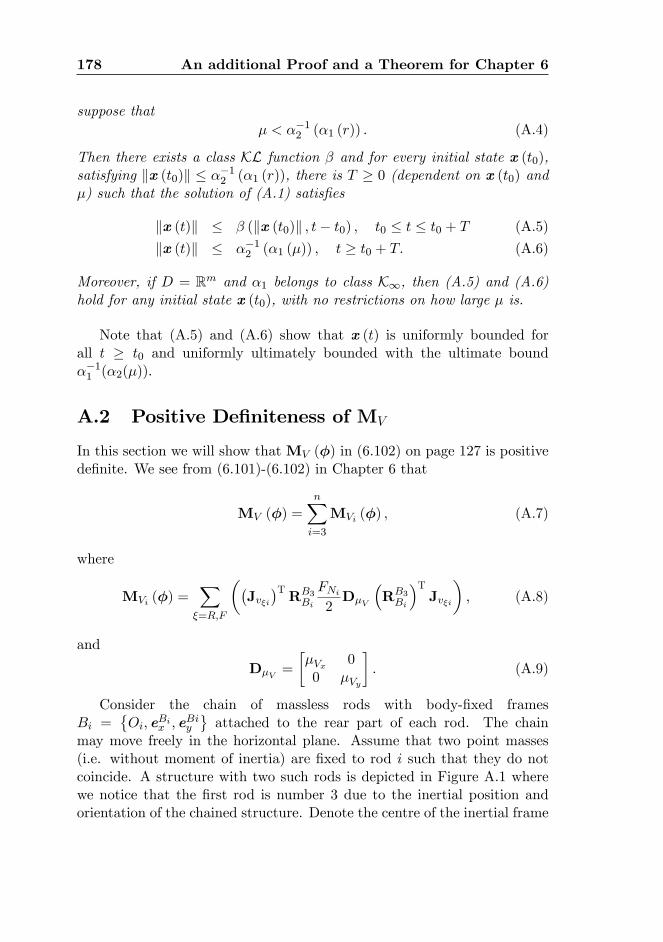
178 An additional Proof and a Theorem for Chapter 6
suppose that� < ��12 (�1 (r)) : (A.4)
Then there exists a class KL function � and for every initial state x (t0),satisfying kx (t0)k � ��12 (�1 (r)), there is T � 0 (dependent on x (t0) and�) such that the solution of (A.1) satis�es
kx (t)k � � (kx (t0)k ; t� t0) ; t0 � t � t0 + T (A.5)
kx (t)k � ��12 (�1 (�)) ; t � t0 + T: (A.6)
Moreover, if D = Rm and �1 belongs to class K1, then (A.5) and (A.6)hold for any initial state x (t0), with no restrictions on how large � is.
Note that (A.5) and (A.6) show that x (t) is uniformly bounded forall t � t0 and uniformly ultimately bounded with the ultimate bound��11 (�2(�)).
A.2 Positive De�niteness of MV
In this section we will show thatMV (�) in (6.102) on page 127 is positivede�nite. We see from (6.101)-(6.102) in Chapter 6 that
MV (�) =
nXi=3
MVi (�) ; (A.7)
where
MVi (�) =X�=R;F
��Jv�i
�TRB3Bi
FNi2D�V
�RB3Bi
�TJv�i
�; (A.8)
and
D�V =
��Vx 00 �Vy
�: (A.9)
Consider the chain of massless rods with body-�xed framesBi =
�Oi; e
Bix ; e
Biy
attached to the rear part of each rod. The chain
may move freely in the horizontal plane. Assume that two point masses(i.e. without moment of inertia) are �xed to rod i such that they do notcoincide. A structure with two such rods is depicted in Figure A.1 wherewe notice that the �rst rod is number 3 due to the inertial position andorientation of the chained structure. Denote the centre of the inertial frame
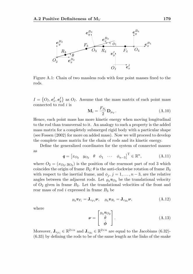
A.2 Positive De�niteness of MV 179
Figure A.1: Chain of two massless rods with four point masses �xed to therods.
I =�OI ; e
Ix; e
Iy
as OI . Assume that the mass matrix of each point mass
connected to rod i is
Mi =FNi2D�V : (A.10)
Hence, each point mass has more kinetic energy when moving longitudinalto the rod than transversal to it. An analogy to such a property is the addedmass matrix for a completely submerged rigid body with a particular shape(see Fossen (2002) for more on added mass). Now we will proceed to developthe complete mass matrix for the chain of rods and its kinetic energy.
De�ne the generalized coordinates for the system of connected massesas
q =�xO2 yO2 � �1 � � � �n�3
�T 2 Rn; (A.11)
where O2 = (xO2 ; yO2) is the position of the rearmost part of rod 3 whichcoincides the origin of frame B2; � is the anti-clockwise rotation of frame B3with respect to the inertial frame, and �j , j = 1; : : : ; n� 3; are the relativeangles between the adjacent rods. Let B3vO2 be the translational velocityof O2 given in frame B3. Let the translational velocities of the front andrear mass of rod i expressed in frame B3 be
B3vFi = JvFi�; B3vRi = JvRi�; (A.12)
where
� =
24B3vO2_�_�
35 : (A.13)
Moreover, JvFi 2 R2�n and JvRi 2 R2�n are equal to the Jacobians (6.32)-(6.33) by de�ning the rods to be of the same length as the links of the snake
180 An additional Proof and a Theorem for Chapter 6
robot presented in Chapter 6 and that the point masses in this section areplaced at the same points as the contact points with the ground de�nedfor the links in Chapter 6. The velocities of the point masses are expressedfrom (A.12) in their corresponding frames as
BivFi =�RB3Bi
�TB3vFi ; BivRi =
�RB3Bi
�TB3vRi ; (A.14)
where RB3Biis the rotation matrix that transforms a velocity vector from
being described in frame Bi to being described in frame B3 by the trans-formation B3vFi = RB3
Bi BivFi . The total kinetic energy K of the chained
structure of connected rods can now be found as
K =
nXi=3
�1
2Biv
TFiMi BivFi +
1
2Biv
TRiMi BivRi
�; (A.15)
and by inserting (A.10), (A.12) and (A.14) into (A.15), we �nd that
K =1
2�T
X�i=Ri;Fi
nXi=3
�(JvFi)
TRB3Bi
FNi2D�V
�RB3Bi
�TJvFi
�| {z }
MK
�: (A.16)
Since the kinetic energy of the system is always positive for k�k 6= 0 wehave that MK is positive de�nite. Moreover, by comparing MV given in(A.7) to MK indicated in (A.16) we see that they are equal. Hence, MV
is also positive de�nite, which concludes the proof.