Embed Size (px)
Citation preview

Contributions to Modelling of InternetTraffic by Fractal Renewal Processes
Muhammad Asad Arfeen
Department of Computer Science & Software EngineeringCollege of Engineering
University of Canterbury
A thesis submitted in partial fulfilmentof the requirements for the degree of
Doctor of Philosophyin
Computer Science
2014

Supervisors
Principal Supervisor:
Emeritus Professor Krzysztof Pawlikowski
Department of Computer Science & Software Engineering
Co-Supervisors:
Associate Professor Donald C. McNickle
Department of Management
Dr. Andreas Willig
Department of Computer Science & Software Engineering

Examination Committee
Examiners:
Emeritus Professor Richard Harris
School of Engineering & Advanced Technology
Massey University, New Zealand.
Professor Franco Davoli
Satellite Communications & Networking Laboratory
University of Genoa, Italy.
Oral Examination Chair:
Associate Professor R. Mukundan
Department of Computer Science & Software Engineering
University of Canterbury.
Principal Supervisor:
Emeritus Professor Krzysztof Pawlikowski
Department of Computer Science & Software Engineering

To my lovely daughter
Safa

Acknowledgements
My research supervisor Emeritus Professor Krys Pawlikowski is not only a mentor
for me in research, but he has also been a mentor for me as a human being. Krys
has always encouraged me towards a scientific contribution, however small or
modest it may be. Krys introduced and guided me towards a broad and very
interesting research area of Internet traffic modelling, for which I am extremely
thankful to him. I am also thankful to Krys for always being a support for me
in difficult times especially during and after the February 2011 Christchurch
earthquake. I am also indebted to my co-supervisor Associate Professor Don
McNickle who has a great input in correcting and streamlining my research.
Don’s constructive comments on my thesis and research publications have been
very valuable. Also many thanks to Dr. Andreas Willig for his guidance and
stimulating research discussions in our research group meetings.
I would like to acknowledge Research and Education Advanced Network New
Zealand (REANNZ) for awarding me PlanetLab New Zealand scholarship. I
am also thankful to G. B. Battersby Trimble fund, International Teletraffic
Congress (ITC) and Australasian Telecommunication Networks and Applications
Conference (ATNAC) for their various research and travel grants towards my
thesis and publications.
I am extremely grateful to Associate Professor Tony McGregor for hosting my
research visits thrice at Waikato Applied Network Dynamics (WAND) research
group of University of Waikato. Shane Alcock of WAND research group has also
been a mentor and good friend for me. Shane helped me in Internet traffic
capturing methodologies and provided me Internet traffic traces of various
access networks, for which I am extremely thankful to him. Also, many thanks
to Brendon Jones and Brad Cowie of WAND. My fellow PhD student Abdul Haq
has been extremely helpful to me whenever I faced problems in programming.
Many thanks to Abdul Haq for introducing me to the capabilities of R. I am also
thankful to Professor Peter Harrison of Imperial College London and Professor
Adam Wolisz of Technical University of Berlin for hosting me in their research

groups during short but very enlightening visits.
I am thankful to New Zealand ICT Innovation Institute (NZi3) for facilitating
my research studies by providing me a nice working space at NZi3 building after
the Christchurch earthquake 2011, when most of the buildings at University
of Canterbury were damaged and shut down for repair. This was indeed an
unexpected time for me both as a researcher and as a human being. During
university closure, I joined the student volunteer team for earthquake related
support activities in various suburbs of Christchurch. I learned to become a
human independent of ethnicity, religion, colour and other social and economical
disparities.
I would like express my profound thanks to a humane person named Aamir
Rehman who acted as a guardian for me ever since he saw me in Christchurch
for the first time. Aamir bhai, his mother Safia Bano amma (RIP) and his sister
Sumera baji were always there for my moral uplift and provided a family like
care to me during all times in Christchurch. Also, especial thanks to Saif and
Furqan.
Lastly, I am extremely thankful to my parents for bringing me up and making
no compromise for my education in all situations. I would like to thank my wife
Aysha who joined my life in the last year of my doctoral research; we are blessed
with a cute baby girl Safa.
I would like to dedicate this thesis to my daughter Safa-my-heart !

PublicationsJournal Publication• Muhammad Asad Arfeen, Krzysztof Pawlikowski, Don McNickle, AndreasWillig, “Internet Traffic Modeling : From Superposition to Scaling”, IET Networks,volume 3, Special Issue on Teletraffic Engineering in Communications Systems,2014.
Conference Publications• Muhammad Asad Arfeen, Krzysztof Pawlikowski, Don McNickle, AndreasWillig, “The Role of the Weibull Distribution in Internet Traffic Modeling”, 25thInternational Teletraffic Congress (ITC 2013), Shanghai, China.
• Muhammad Asad Arfeen, Krzysztof Pawlikowski, Don McNickle, AndreasWillig, “Scaling Analysis of the Internet Traffic Structural Dynamics”, Aus-tralasian Telecommunication Networks and Applications Conference (ATNAC2013), Christchurch, New Zealand.
• Muhammad Asad Arfeen, Krzysztof Pawlikowski, Don McNickle, AndreasWillig, “Towards a Combined Traffic Modeling Framework for Access and CoreNetworks”, Australasian Telecommunication Networks and Applications Confer-ence (ATNAC 2012), Brisbane, Australia.
• Muhammad Asad Arfeen, Krzysztof Pawlikowski, Andreas Willig, “A Frame-work for Resource Allocation Strategies in Cloud Computing Environment”,Proceedings of 35th IEEE Computer Software & Applications Conference Work-shops (COMPSACW 2011), Munich, Germany.

Abstract
The principle of parsimonious modelling of Internet traffic states that a minimal
number of descriptors should be used for its characterization. Until early 1990s,
the conventional Markovian models for voice traffic had been considered suitable
and parsimonious for data traffic as well. Later with the discovery of strong
correlations and increased burstiness in Internet traffic, various self-similar count
models have been proposed. But, in fact, such models are strictly mono-fractal
and applicable at coarse time scales, whereas Internet traffic modelling is about
modelling traffic at fine and coarse time scales; modelling traffic which can be
mono and multi-fractal; modelling traffic at interarrival time and count levels;
modelling traffic at access and core tiers; and modelling all the three structural
components of Internet traffic, that is, packets, flows and sessions.
The philosophy of this thesis can be described as: “the renewal of renewal theoryin Internet traffic modelling”. Renewal theory has a great potential in modelling
statistical characteristics of Internet traffic belonging to individual users, access
and core networks. In this thesis, we develop an Internet traffic modelling
framework based on fractal renewal processes, that is, renewal processes with
underlying distribution of interarrival times being heavy-tailed. The proposed
renewal framework covers packets, flows and sessions as structural components
of Internet traffic and is applicable for modelling the traffic at fine and coarse
time scales. The properties of superposition of renewal processes can be used
to model traffic in higher tiers of the Internet hierarchy. As the framework is
based on renewal processes, therefore, Internet traffic can be modelled at both
interarrival times and count levels.

Contents
Contents ix
List of Figures xiii
List of Tables xvii
1 Introduction 11.1 Importance of Internet Traffic Modelling . . . . . . . . . . . . . . . . . . . . 11.2 Principles of Internet Traffic Modelling . . . . . . . . . . . . . . . . . . . . . 3
1.2.1 Approximations and Assumptions . . . . . . . . . . . . . . . . . . . . 31.2.2 Approaches to Modelling . . . . . . . . . . . . . . . . . . . . . . . . 31.2.3 Specific Issues in Internet Traffic Modelling . . . . . . . . . . . . . . 5
1.3 Internet Traffic Modelling: A Renewed Vision . . . . . . . . . . . . . . . . . 51.4 Problem Formulation . . . . . . . . . . . . . . . . . . . . . . . . . . . . . . . 7
1.4.1 Background . . . . . . . . . . . . . . . . . . . . . . . . . . . . . . . . 71.4.2 Thesis Goals and Contributions . . . . . . . . . . . . . . . . . . . . . 8
1.5 Methodology . . . . . . . . . . . . . . . . . . . . . . . . . . . . . . . . . . . 101.5.1 Packets . . . . . . . . . . . . . . . . . . . . . . . . . . . . . . . . . . 101.5.2 Flows . . . . . . . . . . . . . . . . . . . . . . . . . . . . . . . . . . . 101.5.3 Sessions . . . . . . . . . . . . . . . . . . . . . . . . . . . . . . . . . . 11
1.6 Assumptions . . . . . . . . . . . . . . . . . . . . . . . . . . . . . . . . . . . . 131.7 Description of Traffic Traces . . . . . . . . . . . . . . . . . . . . . . . . . . . 131.8 Limitations . . . . . . . . . . . . . . . . . . . . . . . . . . . . . . . . . . . . 161.9 Thesis Outline . . . . . . . . . . . . . . . . . . . . . . . . . . . . . . . . . . . 171.10 Summary of the Chapter . . . . . . . . . . . . . . . . . . . . . . . . . . . . . 18
2 Towards Modelling of Internet Traffic by Renewal Processes 192.1 Introduction . . . . . . . . . . . . . . . . . . . . . . . . . . . . . . . . . . . . 192.2 Renewal Processes . . . . . . . . . . . . . . . . . . . . . . . . . . . . . . . . 20
2.2.1 Definition . . . . . . . . . . . . . . . . . . . . . . . . . . . . . . . . . 202.2.2 Renewal Process: Interarrival Times and Counts . . . . . . . . . . . . 212.2.3 Renewal Process in Equilibrium . . . . . . . . . . . . . . . . . . . . . 222.2.4 Fractal Renewal Process . . . . . . . . . . . . . . . . . . . . . . . . . 232.2.5 Tests for Renewal Behaviour . . . . . . . . . . . . . . . . . . . . . . . 23
ix

CONTENTS
2.3 Renewal Processes and Dispersion . . . . . . . . . . . . . . . . . . . . . . . 242.4 Self-Similarity and Long-Range Dependence . . . . . . . . . . . . . . . . . . 25
2.4.1 Self-Similarity . . . . . . . . . . . . . . . . . . . . . . . . . . . . . . . 252.4.2 Long-Range Dependence . . . . . . . . . . . . . . . . . . . . . . . . . 27
2.5 Heavy-tailed Distributions . . . . . . . . . . . . . . . . . . . . . . . . . . . . 282.5.1 Pareto Distribution . . . . . . . . . . . . . . . . . . . . . . . . . . . . 282.5.2 Weibull Distribution . . . . . . . . . . . . . . . . . . . . . . . . . . . 302.5.3 Log-normal Distribution . . . . . . . . . . . . . . . . . . . . . . . . . 34
2.6 Superposition . . . . . . . . . . . . . . . . . . . . . . . . . . . . . . . . . . . 352.6.1 Superposed Process . . . . . . . . . . . . . . . . . . . . . . . . . . . 362.6.2 Superposition of Renewal Processes . . . . . . . . . . . . . . . . . . . 372.6.3 Renewal Approximations for Superpositions . . . . . . . . . . . . . . 39
2.7 Renewal Processes and Long-Range Dependence . . . . . . . . . . . . . . . 402.8 Summary of the Chapter . . . . . . . . . . . . . . . . . . . . . . . . . . . . . 42
3 Interarrival Time Models for Internet Traffic 433.1 Introduction . . . . . . . . . . . . . . . . . . . . . . . . . . . . . . . . . . . . 433.2 Source Modelling . . . . . . . . . . . . . . . . . . . . . . . . . . . . . . . . . 45
3.2.1 Sessions, Flows and Packets . . . . . . . . . . . . . . . . . . . . . . . 453.2.2 Infinite Mean and Variance in Source Traffic Interarrival Times : A
Justification . . . . . . . . . . . . . . . . . . . . . . . . . . . . . . . . 483.3 Traffic in Access and Core Networks . . . . . . . . . . . . . . . . . . . . . . . 503.4 Superposition of Fractal Renewal Processes . . . . . . . . . . . . . . . . . . 51
3.4.1 Pareto Superposition Model . . . . . . . . . . . . . . . . . . . . . . . 513.4.1.1 Case I: Infinite Mean and Infinite Variance . . . . . . . . . . 523.4.1.2 Case II: Finite Mean and Infinite Variance . . . . . . . . . . 57
3.4.2 Weibull Superposition Model . . . . . . . . . . . . . . . . . . . . . . 623.5 Modelling Interarrival Times in Access and ISP Core Networks . . . . . . . . 65
3.5.1 Index of Dispersion for Intervals Analysis . . . . . . . . . . . . . . . . 653.5.2 Renewal Approximations and Goodness-of-fit Tests . . . . . . . . . . 68
3.5.2.1 CDF Plot based Goodness-of-fit Tests . . . . . . . . . . . . . 683.5.2.2 Kolmogorov-Smirnov and Quantile Matching Tests . . . . . 79
3.5.3 A Discussion on the Weibull Renewal Approximation . . . . . . . . . 823.5.3.1 On the Cox Character of Weibull Renewal Processes . . . . 83
3.6 Queueing Delay Performance of Interarrival Time Models . . . . . . . . . . . 843.7 Summary of the Chapter . . . . . . . . . . . . . . . . . . . . . . . . . . . . . 91
4 Count Models for Internet Traffic 934.1 Introduction . . . . . . . . . . . . . . . . . . . . . . . . . . . . . . . . . . . . 934.2 Time aggregation of Internet Traffic Counts . . . . . . . . . . . . . . . . . . 944.3 Count Models based on Self-Similarity . . . . . . . . . . . . . . . . . . . . . 102
4.3.1 Fractional Brownian Motion . . . . . . . . . . . . . . . . . . . . . . . 1024.3.2 Fractional Gaussian Noise . . . . . . . . . . . . . . . . . . . . . . . . 1044.3.3 Fractional ARIMA Processes . . . . . . . . . . . . . . . . . . . . . . . 104
x

CONTENTS
4.3.4 Superposition of Heavy-tailed ON/OFF Sources . . . . . . . . . . . . 1064.4 Count Models based on Renewal Processes . . . . . . . . . . . . . . . . . . . 108
4.4.1 Poisson Count Model . . . . . . . . . . . . . . . . . . . . . . . . . . . 1084.4.2 Negative Binomial Count Model . . . . . . . . . . . . . . . . . . . . . 1104.4.3 Weibull Count Model . . . . . . . . . . . . . . . . . . . . . . . . . . . 1114.4.4 Gamma Count Model . . . . . . . . . . . . . . . . . . . . . . . . . . . 1154.4.5 Mittag-Leffler Count Model . . . . . . . . . . . . . . . . . . . . . . . 1164.4.6 Selecting Renewal Count Models for Internet Traffic . . . . . . . . . 117
4.5 Self-Similar Count Models versus Renewal Count Models . . . . . . . . . . . 1184.5.1 Applicability of Self-Similar Count Models . . . . . . . . . . . . . . . 1184.5.2 Applicability of Renewal Count Models . . . . . . . . . . . . . . . . . 120
4.6 Modelling Counts in Access and ISP Core Networks . . . . . . . . . . . . . . 1224.6.1 Assessing Probability Mass for Higher Quantiles . . . . . . . . . . . . 1394.6.2 Closeness Metrics . . . . . . . . . . . . . . . . . . . . . . . . . . . . . 145
4.7 Summary of the Chapter . . . . . . . . . . . . . . . . . . . . . . . . . . . . . 145
5 Scaling Models for Internet Traffic 1475.1 Introduction . . . . . . . . . . . . . . . . . . . . . . . . . . . . . . . . . . . . 1475.2 Burstiness in Internet Traffic . . . . . . . . . . . . . . . . . . . . . . . . . . . 149
5.2.1 Burstiness: Index of Dispersion for Counts Analysis . . . . . . . . . . 1505.2.2 Burstiness: Variance-Mean Analysis . . . . . . . . . . . . . . . . . . . 1525.2.3 Burstiness: Count Models . . . . . . . . . . . . . . . . . . . . . . . . 157
5.3 Scaling in Internet Traffic . . . . . . . . . . . . . . . . . . . . . . . . . . . . 1585.3.1 Background on Global and Local Scaling . . . . . . . . . . . . . . . . 1615.3.2 Global Scaling in Internet Traffic . . . . . . . . . . . . . . . . . . . . 1635.3.3 Local Scaling in Internet Traffic . . . . . . . . . . . . . . . . . . . . . 167
5.4 Superposition and Scaling . . . . . . . . . . . . . . . . . . . . . . . . . . . . 1695.4.1 Fractional Gaussian Noise . . . . . . . . . . . . . . . . . . . . . . . . 1695.4.2 Superposed Pareto Model . . . . . . . . . . . . . . . . . . . . . . . . 1725.4.3 Heavy-tailed Weibull Model . . . . . . . . . . . . . . . . . . . . . . . 176
5.5 Summary of the Chapter . . . . . . . . . . . . . . . . . . . . . . . . . . . . . 179
6 Conclusions & Future Work 1816.1 Thesis Summary . . . . . . . . . . . . . . . . . . . . . . . . . . . . . . . . . 1816.2 On the Tractability of the Proposed Traffic Models . . . . . . . . . . . . . . . 1846.3 Future Work . . . . . . . . . . . . . . . . . . . . . . . . . . . . . . . . . . . . 186
6.3.1 Splitting Process in Internet Traffic . . . . . . . . . . . . . . . . . . . 1866.3.2 Modelling Sessions . . . . . . . . . . . . . . . . . . . . . . . . . . . . 1876.3.3 Queueing Performance Evaluation of the Proposed Models . . . . . . 1886.3.4 Inferring Full Characteristics of Traffic from Partial Measurements . . 1886.3.5 Further Research in Count Data Modelling . . . . . . . . . . . . . . . 1906.3.6 Sequential Estimation of Heavy-tail Index . . . . . . . . . . . . . . . 1916.3.7 Sequential Estimation of the Hurst Parameter . . . . . . . . . . . . . 192
xi

CONTENTS
References 193
xii

List of Figures
1.1 Characteristics of Internet traffic in four modelling regimes. Here LRD meansLong-Range Dependent and SRD means Short-Range Dependent. P, F and Smean Packets, Flows and Sessions, respectively. . . . . . . . . . . . . . . . . 9
1.2 Traffic capture at DSL, Ethernet, Wireless hotspot network and at theirmultiplexing point (ISP core network) of a New Zealand urban ISP. . . . . . 15
2.1 An illustration of deterministic self-similarity by a fern leaf. . . . . . . . . . 262.2 Probability density function of the Pareto distribution. . . . . . . . . . . . . 282.3 Probability density function of the Weibull distribution. . . . . . . . . . . . . 312.4 Probability density function of the log-normal distribution. . . . . . . . . . . 342.5 The process of superposition in terms of interarrival times. . . . . . . . . . . 36
3.1 Plot of log-log complementary Empirical Distribution (EMD) and the corre-sponding (beneath every log-log plot) Pareto quantile-quantile plots for userflow interarrival times. . . . . . . . . . . . . . . . . . . . . . . . . . . . . . . 47
3.2 Case 0 < α ≤ 1 : Effect of the superposition of streams with Pareto dis-tributed heavy-tailed interarrival times on Weibull shape parameter. . . . . . 55
3.3 Interarrival time densities resulting from the superposition of Pareto renewalstreams for K = 0.001. . . . . . . . . . . . . . . . . . . . . . . . . . . . . . . 59
3.4 Interarrival time densities resulting from the superposition of Pareto renewalstreams for K = 1. . . . . . . . . . . . . . . . . . . . . . . . . . . . . . . . . 60
3.5 Empirical mean v.s. equilibrium mean of the superposed interarrival timesobtained from the superposition of Pareto renewal streams. Blue colour lines(smooth curves) represent equilibrium mean; and, red colour lines (non-smooth) represent mean obtained from empirical superposition of Paretotype II streams. . . . . . . . . . . . . . . . . . . . . . . . . . . . . . . . . . . 62
3.6 Interarrival time densities resulting from superposition of Weibull renewalstreams. . . . . . . . . . . . . . . . . . . . . . . . . . . . . . . . . . . . . . . 63
3.7 Index of dispersion for interval (IDI) curves for interarrival time traffic inEthernet, DSL, Wireless hotspot and ISP core networks. . . . . . . . . . . . . 67
3.8 Interarrival times in an Ethernet network (Continued). . . . . . . . . . . . . 693.9 Interarrival times in a DSL network (Continued). . . . . . . . . . . . . . . . 723.10 Interarrival times in a Wireless hotspot network (Continued). . . . . . . . . 743.11 Interarrival times in ISP core network (Continued). . . . . . . . . . . . . . . 77
xiii

LIST OF FIGURES
3.12 Queueing delay analysis for utilization 0.2 . . . . . . . . . . . . . . . . . . . 883.13 Queueing delay analysis for utilization 0.5 . . . . . . . . . . . . . . . . . . . 893.14 Queueing delay analysis for utilization 0.8 . . . . . . . . . . . . . . . . . . . 90
4.1 Multiple time scale fluctuations of outgoing packet counts. . . . . . . . . . . 974.2 Multiple time scale fluctuations of incoming packet counts. . . . . . . . . . . 984.3 Multiple time scale fluctuations of outgoing flow counts. . . . . . . . . . . . 994.4 Multiple time scale fluctuations of incoming flow counts. . . . . . . . . . . . 1004.5 Multiple time scale fluctuations of session counts. . . . . . . . . . . . . . . . 1014.6 Counts in Ethernet network. . . . . . . . . . . . . . . . . . . . . . . . . . . . 1244.7 Counts in DSL network. . . . . . . . . . . . . . . . . . . . . . . . . . . . . . 1294.8 Counts in Wireless hotspot network. . . . . . . . . . . . . . . . . . . . . . . 1314.9 Counts in ISP core network. . . . . . . . . . . . . . . . . . . . . . . . . . . . 134
5.1 Index of dispersion for counts (IDC) curves of traffic in Ethernet, DSL,Wireless hotspot and ISP core networks. . . . . . . . . . . . . . . . . . . . . 151
5.2 Variance-mean plots for session, flow and packet counts in access and ISPcore networks at 100 microseconds time aggregation. . . . . . . . . . . . . . 154
5.3 Variance-mean plots for session, flow and packet counts in access and ISPcore networks at 10 milliseconds time aggregation. . . . . . . . . . . . . . . 155
5.4 Variance-mean plots for session, flow and packet counts in access and ISPcore networks at 200 milliseconds time aggregation. . . . . . . . . . . . . . 156
5.5 A comparison of a sample variance-mean relation for various count models(“mean” denotes the rate parameter). . . . . . . . . . . . . . . . . . . . . . . 157
5.6 Autocorrelation function (ACF) of traffic in Ethernet, DSL, Wireless hotspotand ISP core network at 10 milliseconds time aggregation. . . . . . . . . . . 159
5.7 Autocorrelation function (ACF) of traffic in Ethernet, DSL, Wireless hotspotand ISP core network at 200 milliseconds time aggregation. . . . . . . . . . 160
5.8 Global scaling analysis of session, flow and packet counts. . . . . . . . . . . 1655.9 Analysis of local scaling of the traffic in Ethernet, DSL, Wireless hotspot and
ISP core networks, for first 10 higher moments of wavelet partition function. 1685.10 Global scaling analysis of the Fractional Gaussian Noise (FGN) for different
values of Hurst parameter. . . . . . . . . . . . . . . . . . . . . . . . . . . . . 1705.11 Local scaling analysis of Fractional Gaussian Noise (FGN), for first 10 higher
moments of wavelet partition function, showing strict mono-fractal scalingas Hurst parameter tends to 1. . . . . . . . . . . . . . . . . . . . . . . . . . 171
5.12 Global scaling analysis of the superposition of Pareto renewal traffic streams. 1735.13 Local scaling analysis of the superposition of Pareto renewal traffic streams
for the first 10 higher moments of wavelet partition function. . . . . . . . . 1755.14 Global scaling analysis of the superposition of the Weibull renewal traffic
streams. . . . . . . . . . . . . . . . . . . . . . . . . . . . . . . . . . . . . . . 1775.15 Local scaling analysis of the superposition of Weibull renewal traffic streams
for the first 10 higher moments of wavelet partition function. . . . . . . . . 178
xiv

LIST OF FIGURES
6.1 Internet traffic characteristics and models for access, ISP core and backbonecore networks. P, F and S mean Packets, Flows and Sessions, respectively. . 183
xv

LIST OF FIGURES
xvi

List of Tables
1.1 Summary of packet, flow and session level traffic counts . . . . . . . . . . . 151.2 Summary of packet, flow and session level traffic interarrivals . . . . . . . . 161.3 Summary of byte level traffic . . . . . . . . . . . . . . . . . . . . . . . . . . 16
3.1 Goodness-of-fit tests for session interarrival times . . . . . . . . . . . . . . . 803.2 Goodness-of-fit tests for outgoing flow interarrival times . . . . . . . . . . . 803.3 Goodness-of-fit tests for incoming flow interarrival times . . . . . . . . . . . 813.4 Goodness-of-fit tests for outgoing packet interarrival times . . . . . . . . . . 813.5 Goodness-of-fit tests for incoming packet interarrival times . . . . . . . . . . 813.6 Weibull shape parameter of packet, flow and session interarrival times . . . 82
4.1 Weibull shape parameter of packet, flow and session traffic counts . . . . . . 1234.2 Probability mass: session counts versus count models . . . . . . . . . . . . . 1404.3 Probability mass: outgoing flow counts versus count models . . . . . . . . . 1414.4 Probability mass: incoming flow counts versus count models . . . . . . . . . 1424.5 Probability mass: outgoing packet counts versus count models . . . . . . . . 1434.6 Probability mass: incoming packet counts versus count models . . . . . . . . 144
xvii

LIST OF TABLES
xviii

Chapter 1
Introduction
“ What information consumes is rather obvious: it consumes the attention ofits recipients. Hence a wealth of information creates a poverty of attention,and a need to allocate that attention efficiently among the overabundanceof information sources that might consume it.
”Herbert Simon, Noble Prize winner economist, 1977
1.1 Importance of Internet Traffic Modelling
The survival and prosperity of human society depends on various important facilities
like health care, financial systems, education, entertainment, transportation, security and
communication. In the present era, all of these major services are becoming more and more
operationally dependent on Internet for their accessibility and availability. Therefore, any
disruption or degradation in access to the Internet affects access to these vital facilities.
Internet is now ubiquitous in every aspect of human life to the extent of survivability. To
cater for the growing needs of society, there has been a significant amount of research and
development targeted at increasing the provisioning and capacity of Internet access services.
Broadband Internet access technologies like Gigabit Local Area Networks (LAN), Very-high-
bit-rate Digital Subscriber Lines (VDSL), fibre access networks, wireless hotspot networks,
Wimax and Long Term Evolution (LTE) technologies are part of these efforts.

2 Introduction
Traditional telecommunication services (wired and mobile) are also being replaced by the
quality of service enabled Internet based applications, for example, Skype, Vibre, Whatsapp
and various other multimedia communication applications. The underlying carrier protocol
of Internet is the Internet Protocol (IP) which is a non-guaranteed best effort delivery service
for any kind of data transfer, whether it is a file transfer or an application requiring real time
delivery service. In spite of the insecure and non-guaranteed nature of the Internet packet
delivery protocol, the dependability and trust of our society on the Internet is increasing.
This is mainly due to the low cost structure and the ability of the Internet to provide service
provider- and user-programmable services in a unified framework.
The Internet with its ARPANET origin is less than 50 years old. Now it is impossible to
imagine a world without its services. In 2014, this largest-ever system built by our civiliza-
tion is expected to have over 3 billion users and its further growth will be proportionate
to the world population and its requirements. This is so because access to Internet is now
considered as one of the basic necessities of human life, at least for its prosperity. However,
despite its current significance, the present embodiment of the Internet has approached its
engineering limits. A number of national and international research initiatives have focused
on designing the Future Internet (FI). Some of the projects in this regard are Future InternetForum1, G-Lab project2 and the GENI project3.The Internet in its future shape is expected to
be robust in offering arbitrary information services of the required quality, regardless of the
number of active users or routing devices and their distribution around the globe.
Over 100 years ago, studies of the processes occurring in telephone networks formed
the foundations for the mathematical theory of queues, that allowed engineering large
telephone networks of the 20th century. Now, the intelligent design of the future Inter-
net requires new scientific methodologies, referred to as Internet mathematics, Internet
measurements and Internet statistics [Baccelli, 2008]. In spite of numerous attempts for
developing such methodologies, both by theoretical studies of processes occurring in the
Internet and by statistical investigations of real and simulated data traffic of the Internet, it
is still a long way from a full understanding of the dynamics of these processes, and for
developing mathematical and simulation models that can be used both by scientists and
practitioners in their performance evaluation studies of the current and future incarnations
of Internet and information services they can offer.
1http://www.fif.kr2http://www.german-lab.de3http://www.geni.net

1.2 Principles of Internet Traffic Modelling 3
1.2 Principles of Internet Traffic Modelling
Here we identify some general principles which are useful for developing a model of Internet
traffic.
1.2.1 Approximations and Assumptions
A model is a simplified abstraction of system which captures all or part of its properties.
Various approximations and simplifying assumptions can be used in developing a model.
A careful record of these approximations and assumptions is an essential part of model
formulation and description. This record is necessary due to various reasons [Daellenbach
et al., 2013]:
• To make a model usable by practitioners, simplicity in the model is necessary. Sim-
plicity comes with its own advantages (for example, powerful analytical techniques,
predictability) and limitations which should be recorded so that practitioners are
aware of the model’s capabilities and limitations.
• Approximations and assumptions can be modified to assess change (performance
improvement or degradation) in system behaviour.
• A future modification in a model is not possible without clear understanding of any
approximations and assumptions.
Due to the huge volume of Internet traffic data and its dynamics, Internet traffic modelling
requires various approximations and simplifying assumptions.
1.2.2 Approaches to Modelling
In general there are two main approaches that can be used to derive a model for a system.
Namely, a structural approach and a process approach [Daellenbach et al., 2013].
In the structural approach, the components or all parts of a system are known along with
their controllability, interaction points and boundaries. For example, to study mean delay
experienced by Internet packets at a switch or router, the model structure can be a queue
with a packet processor. Some components of a structural model can be controllable and
others uncontrollable.

4 Introduction
In the process approach, the underlying structure of the system under study is not known
or difficult to observe. Therefore, no prior assumptions can be made about the models
or its components. In this approach, a model is traced by observing the transformation
process between inputs (which can be controlled and uncontrolled) and output(s). In
[Daellenbach et al., 2013], the following four rules are described which are useful in
identifying the components, inputs and outputs of a model derived from a process based
modelling approach:
• Any controllable or uncontrollable aspect, which affects the system behaviour but in
turn is not affected by it, can be treated as model input.
• Any aspect that is only affected by the transformation process either directly or indi-
rectly is a model output provided that it further does not affect any other component
of the system.
• Any aspect which is influenced by inputs and other components of the system and
causes a partial or full change (output) in system behaviour can be treated as a
component or a relationship..
• Any aspect which remains unchanged independent of system dynamics is irrelevant
and can be ignored.
Internet traffic modelling cannot be limited to any one of the above two approaches,
especially when Internet traffic is viewed as a process in itself independent of various
Internet devices (links, routers or switches), which it traverses. Analysis of a traffic trace is
an integral component of Internet traffic modelling and, most of the time, it is unclear how
may links and queues the traffic passed through and under what conditions. Therefore,
a purely structural approach of modelling may not be possible. Nevertheless, it is clear
that Internet traffic is always an active mixture or superposition of Internet traffic streams1
belonging to various users. Using a process based approach, the variants and invariants of
Internet traffic can be identified and assessed in a partial structural framework of modelling.
Moreover, the process based modelling framework ignores the invariants, but in the case
of Internet traffic modelling invariants can play an important role; see [Zhang & Duffield,
2001]. Therefore, Internet traffic modelling is a hybrid combination of the structural and
process based approaches.
1By this term we mean all sorts of data encapsulated and routed by IP; for example, text, voice, video andcontrol data.

1.3 Internet Traffic Modelling: A Renewed Vision 5
1.2.3 Specific Issues in Internet Traffic Modelling
As described above, Internet traffic modelling can benefit from the general approaches
used for system modelling. Nevertheless, there are also specific issues in Internet traffic
modelling which should be considered while developing a model for Internet traffic.
• An important issue in Internet traffic modelling is whether to follow the principle ofparsimony or not. The principle of parsimony favours the model which has a smaller
number of parameters [Andersen & Nielsen, 1998]. Additionally, this principle
requires that a model is simple and universal enough to be applicable in a wide variety
of conditions without requiring too many initial guesses for setting or optimizing the
parameters of the model [Willinger & Paxson, 1998].
• The properties of Internet traffic at fine time scales can be markedly different from the
properties at coarse time scales. It is, therefore, difficult to develop a single unified
model applicable for both fine and coarse time scales.
• A model can succeed in capturing the properties of a real Internet traffic trace, but
it may not capture the observed traffic characteristics from a different traffic trace
[Muscariello et al., 2005]. Therefore, in order for an Internet traffic model to have a
larger domain of applicability, it should have some invariant physical justifications
(for example, based on user access patterns) along with an appropriate mathematical
formulation of any transformation processes faced by Internet traffic.
1.3 Internet Traffic Modelling: A Renewed Vision
Fundamentally, the Internet was designed as a content retrieval network. That is, the
incoming traffic to an access network was significantly higher than the outgoing traffic
because users were meant to act as information sinks (generating no data except requests).
This is no longer the case now. There have been major technological developments like
extensive use of hand-held Internet enabled smart phones or computing devices, an increase
in on-line social networking, and the off-loading of mobile teletraffic data to various wireless
access networks. Therefore, the notion of Internet traffic asymmetry is undergoing a change.
The outgoing traffic originating from access networks to the global Internet is growing
faster in volume than the growth in the volume of incoming traffic. Therefore, the balance
of the traditional Internet traffic asymmetry is undergoing a reverse trend. That is, the

6 Introduction
outgoing traffic may become equal to or even greater than the incoming traffic.
The continuing growth in Internet traffic volume has caused the network over-provisioning
policies to reach near their limitations. Therefore, there has been a renewed interest in
traffic analysis and modelling. With the advent of new access technologies and the increase
in traffic volume originating from access networks, it has become necessary to re-assess
the performance of existing traffic models. The literature on Internet traffic modelling is
divided into two distinct categories. Earlier literature employed classical Markovian models
(for example, Poisson process based models) for both voice and data traffic. Later, with
the discovery of self-similar behaviour in Internet traffic, the models capable of capturing
strong correlations (for example, Fractional Brownian Motion) were proposed.
Classical teletraffic models are based on the notion of the independence of the arrivals
of voice streams. Therefore, they are naturally based on renewal theory and have been
analytically tractable. The classical traffic modelling framework was also extended to the
modelling of Internet traffic until the work of [Paxson & Floyd, 1995], which was based
on new measurements, and questioned the appropriateness of Poisson count models for
packet arrivals in Internet traffic. The measurements in [Paxson & Floyd, 1995; Willinger
& Paxson, 1998] indicated that unlike Poisson counts, the packet arrival counts observed
in Internet traffic traces were not smoothed by time dilation (viewing aggregate traffic at
higher time scales, for example, 1 second, 10 seconds and so on). This phenomenon has
been attributed to the increased burstiness and the persistence of strong correlations in
Internet traffic data over various time scales. The focus of Internet traffic modelling, then,
shifted to self-similar and long-range dependent processes which have the ability to capture
strong correlations and dependencies in the data.
Long-range dependent models like Fractional Brownian Motion (FBM), fractional Gaussian
noise (FGN) and fractional autoregressive processes were proposed as they capture strong
correlations from fine to coarse time scales. LRD models did fit the correlation structure of
Internet traffic at various time scales but they lacked physical justifications. That is, what are
the exact physical mechanisms (for example, bursty or correlated nature of traffic streams or
protocol dynamics), which cause correlation to persist despite aggregation in time and space.
A partial physical justification for a rescaled version of FBM model has been that it results
from the superposition of heavy-tailed ON/OFF traffic sources (resembling traffic generated
from individual users), which converges to FBM in the asymptotic limit [Taqqu et al.,1997]. However, the ON/OFF traffic models focus on second order traffic characteristics
and have been extensively used to model LRD traffic, but they are not appropriate for traffic

1.4 Problem Formulation 7
generation at switching and queueing levels [Riedi et al., 1999].
Moreover, the LRD phenomenon, being asymptotic in nature, also suffers from detection and
estimation issues. That is, various kinds of non-stationarities (for example, a sudden shift
in mean level) can cause false positives in the detection of LRD behaviour. The strength of
the LRD in the traffic data is estimated by evaluating the Hurst parameter, which measures
the persistence effect of the temporal correlations in the data. Several methods to estimate
the Hurst parameter have been proposed (for example, R/S, Whittle’s, Periodogram and
Abry-Veitch’s wavelet based estimators), but they can produce conflicting estimates when
applied to the real and simulated traffic data; see [Karagiannis et al., 2006; Molnar & Dang,
2000; Rea et al., 2013; Ritke et al., 2001], for example.
Interestingly, the classical teletraffic models did not completely lose their applicability. In
[Cao et al., 2003] and [Karagiannis et al., 2004b], comparatively recent Internet backbone
traffic at packet level was investigated and it was reported to be nearly uncorrelated or
short range dependent. A fast decay of correlations was observed due to the high degree
of multiplexing effects in the backbone core network. Thus, depending upon the level of
multiplexing (access or core network) and the statistical behaviour of the traffic streams,
LRD and SRD can coexist at access and backbone core tiers of the Internet hierarchy.
Therefore, there is a need of a traffic modelling framework that can capture a relationship
between LRD and SRD as traffic moves from access to core networks.
1.4 Problem Formulation
1.4.1 Background
Starting from the late nineties, the strong emphasis on LRD based modelling of Internet
traffic has resulted in the over-looking of the capabilities of renewal processes, in spite
of the fact that there have been new developments in renewal theory, especially in the
case of heavy-tailed (fractal) renewal streams; see [Lowen & Teich, 1993; McShane et al.,2008; Mitov & Yanev, 2006], for example. Heavy-tailed distributions are inherent in various
attributes of Internet traffic (for example, in interarrival times, file sizes, count data); see
[Clegg et al., 2010; Leland et al., 1994; Willinger et al., 1997], for example. Therefore, in
this thesis, we exploit the capabilities of renewal processes and propose simple renewal
models for Internet traffic data.

8 Introduction
Renewal processes are simple to use and analytically tractable. In [Grossglauser & Bolot,
1999], it has been emphasized that the marginal distribution of Internet traffic arrival
processes need to be considered for traffic modelling because processes having the same
second order characteristics (strength of auto-correlation or long-range dependence) can
produce contradictory queueing performance [Grossglauser & Bolot, 1999].
The aim of this thesis is to fill the basic gaps in our understanding of the traffic processes
occurring in the Internet. This includes a challenging issue of the formulation of a par-simonious structural model for Internet traffic. The underlying principle of parsimoniousmodelling is to limit the number of parameters used to specify a model [Andersen & Nielsen,
1998]. The objective here is to develop a model which can capture the structural com-
position of Internet traffic at packet, flow and session levels at different time scales. We
also plan to investigate distributional convergence of data streams as they are subjected to
various transformations on their way from access networks to the ISP core and backbone
core networks.
In this thesis, we are mainly focused on developing interarrival time, count and scaling
models for the arrival process of Internet traffic in terms of its structural components, that
is, packets, flows and sessions. The main objective is to develop simple and analytically
tractable models with physical justifications.
1.4.2 Thesis Goals and Contributions
Single and multiple time scale views of Internet traffic count data at fine and coarse time
scales produce four different regimes for Internet traffic modelling. In each of these traffic
modelling regimes, the statistical characteristics of interarrival time and count data of
Internet traffic at packet, flow and session levels can be different. Moreover, as Internet
traffic traverses from an access network to a backbone core network, the statistical profiles
of the traffic in these four regimes can change. Therefore, it is challenging to develop a
single traffic model which can account for the dynamic statistical characteristics of packets,
flows and sessions in these four traffic modelling regimes. A network practitioner is mostly
interested in raw traffic characteristics, that is, traffic characteristics at fine time scales, as
they directly affect network performance at switching or queueing level. In this thesis, we
primarily focus on the single and fine time scale statistical behaviour of Internet traffic for
model development. We also assess and compare coarse and multiple time scale behaviour
of the proposed models with real Internet traffic in access and ISP core networks. The

1.4 Problem Formulation 9
Traffic Characteristics
P=?
F=?
S=?
Traffic Characteristics
P= LRD
F=?
S=?
Traffic Characteristics
P=?
F=?
S=?
Traffic Characteristics
P=?
F=?
S=?
Fine time scales Coarse time scales
Single time
scale view
Multiple time
scale view
Traffic Characteristics
P=Poisson
F=?
S=?
Traffic Characteristics
P=LRD/SRD
F=LRD/SRD
S=LRD/SRD
Traffic Characteristics
P=mono-fratcal
F=multi/mono-fracatl
S=multi/mono-fractal
Traffic Characteristics
P=locally Poisson
F=?
S= ?
Fine time scales Coarse time scales
Single time
scale view
Multiple time
scale view
Traffic in access / ISP core networks Traffic in backbone core network
Figure 1.1: Characteristics of Internet traffic in four modelling regimes. Here LRD meansLong-Range Dependent and SRD means Short-Range Dependent. P, F and S mean Packets,Flows and Sessions, respectively.
main goal of this thesis is to establish a unified and simple framework capable of modelling
Internet traffic belonging to users, access and ISP core network tiers of the Internet hierarchy.
In this direction, this thesis aims at the following contributions:
• Developing a unified traffic modelling framework for characterizing the three struc-
tural components of Internet traffic, that is, streams of packets, flows and sessions.
• Establishing practical models of interarrival times and counts for Internet traffic in
access and ISP core networks, by taking into account the asymptotic properties of
superpositions of fractal renewal processes.
• Analyzing the burstiness and global and local scaling properties of Internet traffic at
packet, flow and session levels in access and ISP core networks. The proposed traffic
models based on fractal renewal processes and their superpositions exhibit a similar
burstiness and scaling behaviour at global and local levels, as that of real Internet
traffic.
Our analysis is unique in the sense that the traffic data analysed in this thesis belong to three
different access networks and their multiplexing in ISP core network. Figure 1.1 presents a
visual clarification of the objectives of this thesis. Based on the available traffic traces, our
analysis applies to access and ISP core networks (left side of Figure 1.1). Nevertheless, using
available theory, we shall also describe the applicability of our results to the Internet traffic
in backbone core networks (right part of Figure 1.1). Here, the term LRD or SRD denotes
long-range or short-range dependence, which refers to the strength of autocorrelations in
traffic. The term locally Poisson means that traffic is Poisson in time intervals smaller than

10 Introduction
the mean interarrival times. The question mark “?” in Figure 1.1 refers to the characteristic
of Internet traffic to be investigated at both fine and coarse time scales. The terminologies
like LRD/SRD, heavy tails and renewal processes, and their applicability in Internet traffic
will be described in Chapter 2.
1.5 Methodology
Packets, flows and sessions are the structural components of Internet traffic. In this section,
the methodologies of identifying packets, flows and sessions from an anonymized traffic
trace are described.
1.5.1 Packets
Physically, Internet traffic consists of streams of packets which carry payload bytes, the
maximum size of which is governed by the Maximum Transmission Unit (MTU) of the
underlying physical medium (wired or wireless). A packet contains an Internet Protocol
(IP) and a transport layer header, that is, a Transmission Control Protocol (TCP) header,
User Datagram Protocol (UDP) or Internet Control Message Protocol (ICMP) header. An
IP header helps in routing of the packet to its destination with the help of IP addresses of
source and destination. A TCP or UDP header helps to deliver the packet to an appropriate
application with the help of source and destination port numbers. Several tools are available
which can help in capturing packets from network interfaces and traffic trace files; see
[Alcock et al., 2012] and references therein, for example. In this thesis, we consider
outgoing packets and incoming packets as a separate series of traffic data.
1.5.2 Flows
Unlike a packet, a flow is not a physical entity. Rather, it is a logical entity which refers to
a series of packets belonging to a source and destination pair with the same IP addresses
and TCP or UDP port numbers. Flows can be classified as TCP or UDP flows separately or
they can be considered irrespective of the transport protocol for a combined analysis. For
the combined analysis, a new flow can be identified on the basis of every newly observed
5-tuple ([source,destination]×[address,port],protocol) in both directions by maintaining a

1.5 Methodology 11
flow table for both directions. In this thesis, we assess both the TCP and the UDP flows in a
combined framework, that is, a flow arrival means an arrival of either a new TCP or a new
UDP 5-tuple in each direction. In this thesis, we treat outgoing flows and incoming flows
separately and independently of each other.
1.5.3 Sessions
A session is a user initiated process. Therefore, we assess it in terms of outgoing traffic only.
The beginning of a user-session marks the starting point of incoming and outgoing flows
and packets all of which belong to that session. The identification of a session faces both
logical and technological challenges. Namely:
• The term session has been perceived differently among researchers. For some, it refers
to the whole duration of one log-in of a user to the Internet. For others, it refers to a
web-page’s browsing duration. For some others, sessions are separated by the long
breaks in the individual user’s activity.
• Unlike layer 4 flows, sessions cannot be identified by a 5-tuple. The only exception
being the sessions having one flow only.
• It is difficult to map sessions quantitatively to flows due to an ever growing application
mix. The number of flows in a session have been reported to be heavy-tailed [Bianco
et al., 2005].
• Application layer traffic classification can help in identification of user sessions but it
is still not a fully solved research problem. Existing traffic classification tools, even
payload based, do suffer from various accuracy and false positives issues; see [Alcock
& Nelson, 2013], for example.
• Grouping flows belonging to a session is also not trivial as the traffic traces contain
both Peer-to-Peer (P2P) and Skype traffic and, for such a traffic, the 5-tuple changes
(these applications do port hopping in the same flow) even for the same flow. Thus, a
single flow can appear as multiple and totally different flows.
• Inter-flow correlations can help identify user sessions as suggested in [Ricciato et al.,2009] and used by us; see [Arfeen et al., 2013]. Such a practice is computationally
expensive and suffers from fuzziness in defining the boundary between “high” and
“low” correlations.

12 Introduction
Both the flow and the super-flow structures (sessions) are important entities in structural
modelling of Internet traffic. Therefore, observing the difficulties in identifying user sessions,
we refer to the TCP session’s outgoing SYN segment, and observe the following:
• From the SYN flag in the header of outgoing packet, the start of a TCP session can be
easily identified without maintaining any flow table.
• The time stamps of outgoing TCP SYN segments keep track of all sessions and sub-
sessions resulting from single application. Long breaks in outgoing TCP SYN segments
can identify user think times.
• Monitoring of TCP SYN segments is an established technique and has been of great
technical importance in congestion control and the identification of denial of service
attacks (TCP SYN flooding).
Therefore, based on the assumption that the time stamp of the outgoing TCP SYN segment
has a one-to-one correspondence with the actual user session arrival time, we propose
to use it as a user-session time stamp. From here on, we use the term session to refer to
an outgoing TCP SYN segment. Even though it is likely that there exists a many-to-one
correspondence between outgoing TCP SYN segments and an actual user session, the
TCP SYN segment arrival process, in itself, is an important engineering component of the
structural modelling of Internet traffic, as well as in various monitoring applications.
It is worth mentioning that a new technique, if implemented in web browsers, makes
our definition of session very close to the actual user- web-browsing-session. Namely,
several HTTP requests can be multiplexed over a single TCP connection to optimize traffic.
An example of such project is SPDY (pronounced as ”SPeeDY”)1, which is a part of new
improvements in the Chrome web browser project. In such a technique, the TCP connection
which is multiplexing related TCP connections initiated by various HTTP requests will
act as a TCP session for a complete user-web-session. Therefore, in such a case the time
stamp of TCP SYN segment can be regarded as time stamp of a user-session with with more
confidence. The preferred web browsers in mobile environment, for example Opera Turbo2,
are already using a single TCP connection for entire website access through cloud based
data compression proxy servers.
1http://www.chromium.org/spdy/spdy-whitepaper2http://www.opera.com/turbo

1.6 Assumptions 13
1.6 Assumptions
Here we list some assumptions which we have used in this thesis.
• Throughout this thesis we use anonymized traffic traces from three different access
networks and their multiplexing in ISP core network. Practically speaking, depending
upon the topological structure of each access network, the corresponding traffic may
traverse through more than one queues in the access network’s switches or routers
before reaching the queue of ISP core network router. Here, we assume a single
queue for every access network and their ISP core network. That is, the traffic from
different access networks traverses through the corresponding queues (whose service
times can be different) before multiplexing at the queue of the ISP core network. The
assumption is appropriate in the sense that a queue can be configured to represent
overall queueing behaviour (for example, delay) of an access network.
• As access network switches or routers are provisioned with large buffers to prevent
packet losses, we further assume that the sizes of the access and ISP core network
queues are unlimited (or infinite).
• As outlined in previous section, flows are identified based on the time stamps of
unique 5-tuples, separately in outgoing and incoming directions. Whereas, sessions
are identified based on time stamps of the outgoing TCP SYN segments.
1.7 Description of Traffic Traces
The traffic traces of an unnamed New Zealand ISP were captured in 2012 by the WAND
Research Group at the University of Waikato. The trace files can be obtained from the
website of Waikato Internet Traffic Archive (WITS)1. A DAG 3.7g card has been used for
packet capture. The DAG card is a high precision network measurement card which has
a packet capturing time resolution of less than one microsecond. See the website for
the details of the DAG project2. The ISP provides Wireless hotspot, DSL and Ethernet
connectivity in an urban environment. The 24 hour traffic was captured on the 20th of
January 2012. The traffic belongs to three different Internet access networks, that is,
Ethernet, DSL and Wireless hotspot networks. All traffic of these three access networks
1http://research.wand.net.nz/wits2http://dag.cs.waikato.ac.nz

14 Introduction
traverses through the ISP core network where it was captured and filtered out into the
respective access network traffic on the basis of IP subnet masks. This has enabled us to
analyse both the separate and multiplexed traffic of the access networks. Figure 1.2 shows
a block diagram of the network configuration used in measurements. We use 30 minutes
traffic segments of Ethernet, DSL and Wireless hotspot networks and their ISP core network,
in a time window from 3pm to 3:30pm of New Zealand Standard Time, for analysis.
To the best of our knowledge this is the first study which reports the results of analysis
of the Internet traffic belonging to three different access networks and their multiplexing
or aggregation point in an ISP core network. The traffic traces archived by the WAND
Research Group at the University of Waikato have been extensively used world-wide for
research purposes. The traffic traces of WITS archive are also mirrored at RIPE Network
Coordination Centre (NCC)1 and Center for Applied Internet Data Analysis (CAIDA)2.
It is relevant here to look at general representativeness of traffic traces used in this study.
Internet traffic in other parts of world can be different and may not be fully compatible
with the profile of traffic traces obtain from a New Zealand urban city. A major change in
characteristics of Internet was caused by emergence of Peer-to-Peer services (such as Bit-
Torrent) which evolved during 2000 to 2009; see [Karagiannis et al., 2004a], for example.
Recently it has been reported that the Peer-to-Peer traffic is experiencing a significant
decrease in volume. In [Maier et al., 2009], traffic from 20,000 European residential DSL
customers was assessed and it is reported that “HTTP, not peer-to-peer, traffic dominates by
a significant margin”. A similar observation has been made in the USA [Erman et al., 2009].
In New Zealand, due to enforcement of CAA (Copyright Amendment Act 2011), the use of
P2P traffic has been significantly reduced; see [Alcock & Nelson, 2012].
In fact, properties of traffic in different parts of the world can be different and they are
based on various factors, including the size of population, user interests etc. Nevertheless,
it can be observed that HTTP traffic is still dominant and will continue to be dominant as
various services are being implemented over HTTP. Therefore, we believe that traffic traces
used in this study are representative for a typical Internet traffic in an access or ISP core
network. Nonetheless, we believe that traffic modelling is not a data fitting exercise in its
entirety. We have tried to find invariants and used theory of superposition for developing
traffic models. Therefore, even if our traffic traces are not completely representative, the
proposed models will continue to be relevant for modelling Internet traffic in other parts of
1https://labs.ripe.net/datarepository/data-sets2http://www.caida.org/data/external

1.7 Description of Traffic Traces 15
Figure 1.2: Traffic capture at DSL, Ethernet, Wireless hotspot network and at their multi-plexing point (ISP core network) of a New Zealand urban ISP.
the world.
It is important to note that traffic analysis at two different tiers of Internet hierarchy,
that is at access networks and ISP core network did help us in understanding a relevant
superposition theory and its implications for future network traffic modelling.
Our study is based on the traffic traces archived by WAND group because of their availability.
These traces have been used by many researchers world wide.
Tables 1.1, 1.2 and 1.3 show the packet count, interarrival time and byte count level statistics
corresponding to Ethernet, DSL, Wireless hotspot and their ISP core network. It should be
noted that here the term outgoing refers to the traffic (packets, flows or sessions) originating
from subscribers of access networks to global Internet, and the term incoming refers to
traffic coming from global Internet to access networks. Statistically speaking, outgoing
traffic results from superposition of multiple streams of data and incoming traffic faces
splitting in substreams in ISP core network. In this thesis, we are mainly concerned with
traffic modelling in terms of superposition process. Nevertheless, we have also presented
empirical analysis for the incoming traffic (splitted traffic) as well.
Table 1.1: Summary of packet, flow and session level traffic counts
Traffic volume (M=106, K=103)
Access networks Outgoing packets Incoming packets Outgoing flows Incoming flows Sessions
Ethernet 27.68M 40.72M 942K 612K 361KDSL 14.96M 22.38M 449K 145K 288KWireless hotspot 3.894M 5.783M 92K 26K 58K
ISP core network 46.54M 68.89M 1.484M 784K 708K

16 Introduction
Table 1.2: Summary of packet, flow and session level traffic interarrivals
Mean interarrival times (milliseconds)
Access networks Outgoing packets Incoming packets Outgoing flows Incoming flows Sessions
Ethernet 0.065 0.044 1.9 2.9 4.9DSL 0.12 0.08 4.0 12.0 6.2Wireless hotspot 0.4 0.3 19.5 67.0 30.7
ISP core network 0.039 0.1 1.2 2.3 2.5
Table 1.3: Summary of byte level traffic
Traffic volume (GB)
Access networks Outgoing Incomingbytes bytes
Ethernet 10.07 31.53DSL 3.17 20.82Wireless hotspot 0.969 4.5
ISP core network 14.22 56.87
1.8 Limitations
Here we present some limitations of the work in this thesis.
• Throughout this thesis, we define time stamp of a session as the time stamp of outgoing
TCP SYN segment. A TCP session will be, of course, a more suitable term here. In the
absence of any standard definition of session and methodology to identify it, we refer
to outgoing TCP SYN segment as start of a user session. An actual application layer
session can have more than one outgoing TCP sessions. Therefore, the actual number
of user-session counts will be less than what we have reported in this thesis.
• We treat both incoming flows and outgoing flows independent of each other. Such a
methodology can have both pros and cons in various applications.
• We have assessed queueing performance of the proposed models assuming buffers
of infinite capacity since we were interested in approximated results only. Access
networks have switches and routers with interfaces having large buffers which are,
nonetheless, are finite in capacity. Due to legal restrictions, the technical information
of Internet service provider’s infrastructure and user identities are kept confidential.

1.9 Thesis Outline 17
1.9 Thesis Outline
This thesis is organized as follows. In Chapter 1, we have discussed the need for an appro-
priate unified modelling framework of Internet traffic . We have outlined the governing
principles to be used in Internet traffic modelling. We have presented the problem formu-
lation with thesis objectives and contributions. The methodology of Internet traffic data
analysis, underlying assumptions and limitations of this thesis work are also discussed.
The access networks, their traffic traces used in thesis are also described along with their
representativeness.
Chapter 2 develops the main direction of the thesis by describing renewal processes and
their importance in Internet traffic modelling. The theory of renewal process and long-
range dependence is described. Various heavy-tailed distributions and their role in renewal
processes generating long-range dependent count data is described. The theory of superpo-
sition is explained in terms of interarrival times and count data. Renewal approximations
for a non-renewal superposed output process are also described.
In Chapter 3 a brief survey of models of source, access and backbone core network level
traffic is given. A heavy-tailed superposition model with both approximate renewal and
non-renewal output is developed with the objective of developing a unified traffic modelling
framework. An extensive analysis of interarrival time data at session, outgoing and incoming
flow and packet level, belonging to the various access networks and their ISP core network,
is presented. The fitness and approximation capabilities of various heavy-tailed renewal
models like Weibull, log-normal and exponential are described. A discussion on the utility of
the heavy-tailed Weibull distribution is also presented. Finally, the queueing performance of
the proposed models and the traffic traces (under the assumptions described in the section
1.6) is presented for various utilization levels, for both the exponential and deterministic
servers.
In Chapter 4, a multiple time scale fluctuating behaviour of traffic at packet, flow and session
count level is described. A brief survey of various self-similar and renewal count models is
presented. Limitations of self-similar count models are outlined with an explanation of how
renewal count models overcome them. Performance of various renewal count models is
assessed with respect to Internet traffic and it has been found that the heavy-tailed Weibull
count model provides a good fit to Internet traffic count data distribution. Moreover, it
is flexible enough to capture non-Poisson characteristics of Internet traffic count data at
packet, flow and session levels.

18 Introduction
In Chapter 5, scaling models of Internet traffic have been developed. The concept of
burstiness, and global and local scaling have been defined in appropriate contexts. A
multiple time scale analysis of the burstiness in Internet traffic count data is presented with
the observation that at lower time scales the variance-mean relation is linear, as compared
to higher time scales where it becomes quadratic. This supports the application of fractal
renewal models (for example, heavy-tailed Weibull) at lower time scales. The global and
local scaling properties of structural components of the Internet traffic in access and ISP
core networks are analysed. Also, the global and local scaling properties exhibited by the
earlier proposed multiplexing models and heavy-tailed Weibull renewal models have been
described and their correspondence with Internet traffic data has been established for all
the three structural components of Internet traffic.
Finally, Chapter 6 presents conclusions of the thesis with a description of the avenues of
future research.
1.10 Summary of the Chapter
Internet traffic modelling has been a challenging and an active area of research since many
decades. The dependence of human society on Internet to the extent of survivability will
keep this area always active in research. Internet traffic can exhibit drastically different
characteristics from time to time and from region to region. Different models can capture
different properties of Internet traffic under specific conditions but may not capture other
properties of Internet traffic belonging to the same or different traffic traces. This thesis is
an effort towards developing a unified, simple, structural (for packets, flows and sessions)
and analytically tractable model for Internet traffic that can find its applicability in most of
traffic situations.
Internet traffic modelling can benefit from the general principles of mathematical modelling
of a system. A hybrid of structural and process based modelling approaches is suitable
for developing models of Internet traffic. However, it should be noted that Internet
traffic modelling has its own specific issues which should be considered when developing
models.

Chapter 2
Towards Modelling of Internet Traffic byRenewal Processes
“ In a system of material particles under the influence of forces which dependsonly on spatial coordinates, a given initial state must, in general, recur, notexactly, but to any desired degree of accuracy, infinitely often, provided thesystem always remains in the finite part of the phase space.
”Chandrasekhar, 1943
2.1 Introduction
Internet traffic structurally consists of packets, flows and sessions which can be represented
as events in a point process framework. Modelling of interarrival times of these events
and their counts is the primary objective of Internet traffic modelling. The modelling of
interarrival time data and count data can be done independently of each other. Such an
approach can result in different models. For example, fractional Gaussian noise (FGN) has
been proposed as an Internet traffic model for packet counts per unit time interval. FGN is
a model for count data with no specification of the distribution of underlying interarrival
times. Several methods to infer interarrival times from the FGN based count data have
been proposed, which result in different interarrival time models; see [Paxson, 1997], for

20 Towards Modelling of Internet Traffic by Renewal Processes
example. These interarrival time models correspond to the same FGN count data, but they
are stochastically different and can produce different queueing behaviours.
The advantage of the framework of renewal processes is that it allows a joint modelling
of interarrival times and associated count data. Although this framework is based on a
restrictive assumption of the independence of interarrival times of events which, nonetheless,
should not undermine its utility in Internet traffic modelling. A variety of statistical
distributions is available for modelling interarrival times which can generate a variety of
counting processes useful in Internet traffic modelling.
This chapter is organized as follows. Section 2.2 introduces the concept of renewal processes
and tests for confirming renewal behaviour. In Section 2.3 the count data dispersion
properties of renewal processes is discussed. The Section 2.4 defines the concept of
stochastic self-similarity and long-range dependence. In Section 2.5, various heavy-tailed
distributions are described with their applicability in Internet traffic modelling. In Section
2.6, the process of superposition is described along with its relation to renewal processes.
Section 2.7 describes the long-range dependence in counts generated by certain types of
renewal processes. Finally, Section 2.8 presents a summary of the chapter.
2.2 Renewal Processes
2.2.1 Definition
A Poisson process is a counting process for which the corresponding interarrival times of
events are independent and represent identically distributed exponential random variable.
A renewal process can be considered as a generalisation of the distribution of the interarrival
times corresponding to a Poisson process by relaxing it to be any arbitrary continuous
distribution (that is, not necessarily an exponential distribution). For example, a Weibull
renewal process is a renewal process where interarrival times are drawn from the Weibull
distribution.
More specifically a renewal process can be defined as a counting process {N(t), t > 0} which
counts the total number of renewals till time t with interarrival times being non-negative
random variables X1, X2, · · · , Xn drawn from a continuous probability distribution.
The term renewal in a renewal process is context dependent and generally speaking it
refers to arrival of an event. In reliability analysis the term renewal refers to failure of a

2.2 Renewal Processes 21
device and interrenewal time refers to the life time of a device. In Internet traffic, the term
renewal refers to the arrival of a packet, flow or session. From here on, we will use the term
interarrival times when referring to interrenewal times.
2.2.2 Renewal Process: Interarrival Times and Counts
Let Xi be a random variable denoting the ith interarrival time. Then we can define Sn to be
the time to the nth renewal event, that is:
S0 = 0, Sn =n
∑i=1
Xi, n>1.
That is, S1 is the time of the first renewal event; S2 = X1 + X2 is the time to the second
renewal event and so on. As Sn denotes the time to the nth renewal, therefore, the renewal
counting process N(t) can also be defined as
N(t) = max{n : Sn6t}. (2.1)
This means that the total number of renewal events by time t is greater than or equal to nprovided that the nth renewal occurs occurs before or at time t. This correspondence can be
written in terms of number of renewal events as
N(t)>n ⇐⇒ Sn6t. (2.2)
Therefore, the distribution of N(t) can be written as
P[N(t) = n] = P[N(t) > n]−P[N(t) > n + 1]. (2.3)
Alternatively,
P[N(t) = n] = P[Sn 6 t]−P[Sn+1 6 t]. (2.4)
Since the interarrival time random variables Xi are independent and are drawn from a

22 Towards Modelling of Internet Traffic by Renewal Processes
common continuous distribution function F, therefore the distribution of Sn is Fn, which is
an n-fold convolution of interarrival time distribution F with itself. Therefore, Equation 2.4
can be written as
P[N(t) = n] = Fn(t)− Fn+1(t). (2.5)
The above equation can be used to derive the expression for probability mass function of the
counts of a renewal process based on any continuous time distribution for the interarrival
times. For example, the convolution of exponential random variables leads to Gamma
distribution and by substituting the distribution function of Gamma distribution in Equation
2.5, we get the Poisson counting process as follows.
The n-fold convolution of an exponential random variable with its distribution function
1− e−λt is given as
Fn(t) = 1−n−1
∑i=0
(λt)i
i!e−λt. (2.6)
Substituting Fn and Fn+1 in Equation 2.5, we obtain
P[N(t) = n] =(λt)n
n!e−λt, (2.7)
which is, in fact, a Poisson renewal counting process. It should be noted that unlike the
exponential distribution, a closed form expression for the convolution of other continuous
time distributions may or may not exist. Therefore, the renewal counting processes corre-
sponding to other continuous distributions may not be simple as there can be iterative steps
to calculate their respective n-fold convolutions; see, [Rinne, 2008], for example.
2.2.3 Renewal Process in Equilibrium
A renewal process is said to be an equilibrium renewal process if it has been started and
considered far away from its time origin, as compared to the mean time between its renewal
events. It should be noted that a renewal process can be started from arrival of an event
and then taken far in time to establish it in equilibrium [Cox & Smith, 1954].

2.2 Renewal Processes 23
2.2.4 Fractal Renewal Process
Fractal renewal process is defined as a renewal process based on heavy-tailed interarrival
time distribution. We allow all heavy-tailed distributions, whether they have infinite or
finite moments, in our formulation of fractal renewal processes. Such renewal processes
are called fractal because they can produce counts with strong correlations. Examples of
fractal renewal processes are renewal processes based on interarrival times following Pareto,
Weibull (shape parameter less than 1) and log-normal distributions. These distributions are
described in Section 2.5 along with their applicability in Internet traffic modelling.
2.2.5 Tests for Renewal Behaviour
A fairly general and qualitative approach to assess the strength of renewal behaviour of a
point process is to look for fluctuations or smoothness in the index of dispersion for intervals
and counts which are dimensionless quantities [Torab & Kamen, 2001].
The index of dispersion for intervals (IDI), I(k), is defined as
I(k) =Var(X1 + X2 + . . . + Xk)
kE(X)2 , k = 1, 2, . . ., (2.8)
where Xk denotes the kth interarrival time. For a renewal process, the value of index of
dispersion for intervals remains constant (that is, equal to Var(X)/E(X)2) for all values of
k.
Alternatively, the index of dispersion for counts (IDC), It, is defined as
It =Var(Nt)
E(Nt), (2.9)
where Nt denotes the number of counts in a time interval of length t. It should be noted
that in limit, the IDI and IDC are equal, that is, limk→∞ I(k) = limt→∞ I(t).
Indices of dispersion for intervals and counts are dimensionless quantities, that is, their
estimation does not depend on the dimension of the respective variables. These indices
have been introduced to assess variability or burstiness of arrival processes; see [Gusella,
1991], for example.

24 Towards Modelling of Internet Traffic by Renewal Processes
2.3 Renewal Processes and Dispersion
Arrival of a packet, flow or session are events in Internet traffic. These events can form
statistically dependent or independent arrival processes. This statistical dependence is
caused by any or both of the two phenomena described as follows. That is, the dependence
can be caused by correlated arrivals of events or non-exponential duration between arrivals
of successive events. This statistical dependence is called arrival dependence (also referred
to as occurrence dependence) or duration dependence, respectively.
In the case of arrival dependence, the probability of an arrival depends on previous event
arrivals. Count models with arrival dependence can display contagion which can be positive
or negative. If arrival of an event increases the probability of arrival of the next event,
then the count model is said to display positive contagion. Positive contagion results in
overdispersion (that is, variance of counts exceeds its mean). On the other hand, if arrival of
an event decreases the probability of arrival of the next event, then the count model is said
to exhibit negative contagion. Negative contagion causes underdispersion (that is, variance
of counts is less than its mean). In case of underdispersion, a greater number of counts is
clustered around their mean. An example of a count model with arrival dependence based
on positive contagion is the negative binomial count model.
Duration dependence can also generate various types of dispersion in count data. Duration
dependence refers to the distribution of interarrival time between events which are indepen-
dent but not necessarily exponentially distributed. Duration dependence can be assessed in
terms of hazard rate h(t), which is defined as the ratio of probability density function of
interarrival times and its complementary cumulative distribution function, that is,
h(t) =f (t)
1− F(t). (2.10)
Exponential distribution has a constant hazard rate which means equidispersion. If the
hazard rate is an increasing function of time, then the interarrival time distribution displays
positive duration dependence which leads to underdispersion. Whereas, if the hazard
rate is a decreasing function of time, then the interarrival time distribution will generate
overdispersed counts. For example, the Weibull distribution can exhibit both positive and
negative duration dependence based on the values of its shape parameter.
The following theorem is due to [Winkelmann, 1995].

2.4 Self-Similarity and Long-Range Dependence 25
Theorem 1 1 The negative (positive) duration dependence in interarrival time distributioncauses over(under)-dispersion in the distribution of corresponding count data.
Internet traffic is mostly overdispersed in access networks and tends towards equidispersed
as the level of traffic multiplexing increases [Cao et al., 2003].
2.4 Self-Similarity and Long-Range Dependence
The behaviour of Internet traffic under time rescaling is necessary to understand for
performance evaluation of networks at macro level (higher time scales). Namely, traffic
management and control actions like buffering or bandwidth provisioning are based on
rescaled traffic processes. Here, we briefly explain the notion of self-similarity and long-
range dependence
2.4.1 Self-Similarity
The notion of self-similarity can be deterministic or stochastic in nature. Deterministicself-similarity is restricted to a geometrical sense and can be defined as if an object or
data looks exactly similar when the same self is viewed at different time scales or ag-
gregation levels. The notion of deterministic self-similarity needs to be generalized for
traffic modelling purposes where stochastic measures are essential components. Therefore,
stochastic self-similarity refers to the relaxation of the strict recursive regularity condition
of deterministic self-similarity to similarity in stochastic measures (for example, variance,
autocorrelation).
Scale invariance or scaling is an important phenomenon which makes a process stochasticallyself-similar. To formulate it, we first define the aggregated process or aggregated time series
X(m)(i) of a stochastic process X(t) as
X(m)(i) =1m
mi
∑t=m(i−1)+1
X(t), i > 1, (2.11)
where m is the aggregation level which controls the size of non-overlapping blocks or time
intervals of the time series where averaging is performed and i is the block index. The
1The theorems in this thesis are numbered independent of the source and starts from the number 1.

26 Towards Modelling of Internet Traffic by Renewal Processes
(a) Aggregation level m=1 (b) Aggregation level m=2 (c) Aggregation level m=3
Figure 2.1: An illustration of deterministic self-similarity by a fern leaf.
process X(t) can be interpreted as the number of packets or bytes per unit time interval.
The process X(t) will be stochastically self-similar if it satisfies the following distributional
equality
X d= m1−HX(m), (2.12)
where H is the index of self-similarity called the Hurst parameter. The Hurst parameter is a
second-order scaling exponent which is used to measure the strength of autocorrelation in
the time series or data generated by the process X(t).
Figure 2.1 illustrates the concept of deterministic self-similarity and interpretation of m (in
terms of aggregation in space) in Equation 2.12.
A both qualitative and quantitative method to assess LRD and its onset is the Log-scale
Diagram plot (called LD plot), which has been described in [Abry et al., 1998].

2.4 Self-Similarity and Long-Range Dependence 27
2.4.2 Long-Range Dependence
A process X(t) will be second order self-similar or Long-Range Dependent (LRD) if
m1−HX(m) has the same variance and autocorrelation as X for all values of aggregation
level m.
The autocorrelation function of an LRD process decays hyperbolically, that is:
γ(k) ∼ H(2H − 1)k2H−2, k→ ∞. (2.13)
Here γ(k) is the autocorrelation coefficient at lag k, and H is the Hurst parameter. For
the Hurst parameter in the range 1/2 < H 6 1, γ(k) asymptotically behaves as ck−β for
0 < β < 1, where c > 0 is a constant and β = 2− 2H.
Equation 2.13 can also characterize an LRD process in terms of its sum of autocorrelation
coefficients. Namely, for an LRD process, the autocorrelation coefficients at various lags are
non-summable, that is,
∞
∑k=−∞
γ(k)→ ∞. (2.14)
Equation 2.14 can be used as a definition of an LRD process but it does not tell much about
the specific autocorrelation structure of an LRD process. Whereas, Equation 2.13 gives
more information about the autocorrelation structure of an LRD process. That is why, it is a
more widely used definition of an LRD process.
The Hurst parameter of an LRD process lies in the range 1/2 < H 6 1. For short range
dependent processes (whose autocorrelation function decays fast and its coefficients are
summable), the value of the Hurst parameter is 1/2. For the range 0 < H < 1/2, the
sum of auto correlation function coefficients at all lags tends to zero. This is a case of
anti-persistence and has been rarely found in practical applications.
A commonly used LRD model for Internet traffic is Fractional Brownian Motion (FBM).
The definition and a critical overview of FBM based modelling of Internet traffic will be
described in Chapter 4.

28 Towards Modelling of Internet Traffic by Renewal Processes
0.0 0.5 1.0 1.5 2.0 2.5 3.0
01
23
4 α=0.5, a=1.0
α=1.0, a=1.0
α=1.5, a=1.0
α=2.0, a=1.0
α=3.0, a=1.0
α=4.0, a=1.0
X
fX(x
)
Pareto type I distribution
(a)
0.0 0.5 1.0 1.5 2.0 2.5 3.0
01
23
4 α=0.5, K=1.0
α=1.0, K=1.0
α=1.5, K=1.0
α=2.0, K=1.0
α=3.0, K=1.0
α=4.0, K=1.0
X
fX(x
)
Pareto type II distribution
(b)
0.0 0.5 1.0 1.5 2.0 2.5 3.0
01
23
4 α=0.5, K=2.0
α=1.0, K=2.0
α=1.5, K=2.0
α=2.0, K=2.0
α=3.0, K=2.0
α=4.0, K=2.0
X
fX(x
)
Pareto type II distribution
(c)
Figure 2.2: Probability density function of the Pareto distribution.
2.5 Heavy-tailed Distributions
Continuous valued heavy-tailed distributions are related to LRD in count data [Park &
Willinger, 2002]. In this section, we define and briefly explain some important heavy-tailed
distributions.
Let X1, X2, ..., Xn be a sequence of n independent and identically distributed observations
with the cumulative distribution function F which is heavy-tailed, if it satisfies:
1− F(x) = L(x)x−α, α > 0, x → ∞. (2.15)
Here, L(x) > 0 is a slowly varying function at infinity, and α > 0 is the tail index which
controls the rate of decay of F. In general, if the rate of decay of F is slower than exponential,
then F is called a heavy-tailed distribution. Hence, the value of tail index characterizes the
tail behaviour and contains useful information about extremes of the distribution.
Some commonly used heavy-tailed distributions are Pareto, Weibull and log-normal distri-
butions. Here, we present a brief statistical profile of these heavy-tailed distributions and
their applicability in Internet traffic modelling.
2.5.1 Pareto Distribution
Pareto distribution is one of the simplest and commonly used heavy-tailed distribution in
Internet traffic modelling. All moments of the Pareto distribution can be infinite, which

2.5 Heavy-tailed Distributions 29
makes it useful in modelling interarrival times which generate LRD counts similar to LRD
exhibited by Internet traffic count data. This is due to the fact that the infinite mean or
infinite variance interarrival times can generate highly correlated counts. Interarrival times
in a single user’s sessions and flows may have excessively long values (for example, due to
user think times). Therefore, the Pareto distribution can also be used to model interarrival
times at session and flow levels of individual user or traffic source.
The Pareto type I distribution has probability density function given by
f (x) =
{α aα
xα+1 , x≥a > 0,0 , x < a;
(2.16)
where a is the scale parameter and α > 0 is the tail index which controls the rate of decay of
Pareto probability density function. Figure 2.2(a) shows the probability density function of
the Pareto type I distribution. Pareto distribution has infinite mean and infinite variance for
the tail index range 0 < α ≤ 1, and has finite mean and infinite variance for the tail index
range 1 < α ≤ 2. Variance, skewness, ex-kurtosis and other higher moments start becoming
finite as the value of tail index increases in integer steps (α > 2, α > 3,α > 4, . . .).
Another useful form of Pareto distribution is the Pareto type II distribution (also called as
Lomax distribution) which, unlike Pareto type I, has support on zero. The density function
of the Pareto type II distribution is given as ([Abd-El-Hakim & Sultan, 2004])
f (x) =
{αKα(x + K)−α−1 , x≥0,0 , otherwise;
(2.17)
where K is a normalization constant. Figures 2.2 (b) and (c) show the probability density
function of Pareto type II distribution for different values of α and K. It should be noted
that the Pareto type II distribution is more general than Pareto type I in modelling tail parts
of distribution. The tail of the Pareto type II distribution can be controlled through two
parameters, that is, the tail becomes heavier as K increases and α decreases. Whereas, in
the Pareto type I distribution, the tail is controlled using α only.
Compared with the type II, the type I form of the Pareto distribution has been extensively
used in describing Internet user’s access patterns. Nevertheless, the type II form of the
Pareto distribution has a larger domain with support on zero which makes it applicable in

30 Towards Modelling of Internet Traffic by Renewal Processes
modelling interarrival times in the components and superposed output of a superposition
process. Whereas, the Pareto type I distribution, in its standard non-rescaled form, cannot
be used to model interarrival times in the superposed output because it has no support on
zero.
It should be noted that if X is from the Pareto type I distribution with parameters α and
a, then Y = K(X/a− 1) follows the Pareto type II distribution with parameter α and K[Fishman & Adan, 2006]. We shall discuss the applicability of the Pareto type II distribution
in the Chapter 3.
2.5.2 Weibull Distribution
The Weibull distribution has been extensively used in reliability analysis for the study of
life times. The first study using the Weibull distribution in Internet traffic modelling can be
found in [Feldmann, 2002]. Accordingly, the heavy-tailed Weibull distribution can capture
short as well as long interarrival times of TCP connections of data sources and multiplexed
traffic.
The Weibull distribution has the probability density function given by
f (x) =
{cb( x
b)c−1 e−(x/b)c
, x≥0,0 , x < 0;
(2.18)
where c is a shape parameter and b is a scale parameter. The Weibull distribution is quite
flexible and can represent different shapes of the body and tail parts of a data distribution
based on the value of the shape parameter as shown in Figure 2.3. Exponential and Rayleigh
distributions are special cases of the Weibull distribution. Maximum Likelihood Estimates
(MLE) of the shape parameter c and the scale parameter b can be obtained by the solution
of the following simultaneous equations [Qureishi, 1964]:
c =n
1b ∑n
i=1 xci log xi −∑n
i=1 log xi, (2.19)
and
b =
[1n
n
∑i=1
xci
]1/c
. (2.20)

2.5 Heavy-tailed Distributions 31
0.0 0.5 1.0 1.5 2.0 2.5 3.0
0.0
0.5
1.0
1.5
2.0
c=0.5, b=1.0
c=1.0, b=1.0
c=1.5, b=1.0
c=2.0, b=1.0
c=3.0, b=1.0
c=4.0, b=1.0
X
fX(x
)
Weibull distribution
Figure 2.3: Probability density function of the Weibull distribution.
MLEs are asymptotically normal, therefore, the confidence intervals of the estimate can be
derived by using the normal approximation.
It should be noted that, apart from maximum likelihood estimators, there are also other
methods to estimate model parameters from experimental data. Namely, one can apply the
method of moments or the method of percentiles (quantiles).
The method of moments is the oldest method to estimate parameters from an experimental
data set if one wants to fit the parametric distribution to the data set. The idea here is to
equate sample moments to the theoretical moments of the distribution and solve for the
parameters. Clearly as many moments are required as there are number of parameters to
be estimated.
Suppose µ′r; r = 1, 2, . . . be the r moments about zero of a distribution function and µ′r be
the corresponding sample moments obtained from data as follows,
µ′r =1n
n
∑i=1
Xir. (2.21)

32 Towards Modelling of Internet Traffic by Renewal Processes
Hence the method of moments can be used to estimate model parameters from data
by equating µ′r to µ′r and solving the resulting set of simultaneous equations. For the
2-parameter Weibull distribution, the first two moments are given as,
µ′1 = bΓ(1 + 1/c), (2.22)
µ′2 = b2Γ(1 + 2/c). (2.23)
It should be noted that the method of moments for parameter estimation from experimental
data is not an optimization technique. Moments estimators are asymptotically normal and
consistent, but they are not efficient nor sufficient [Rinne, 2008].
The method of percentiles (also known as the method of quantiles) is similar to the method
of moments. Here, the moments are replaced by percentiles (quantiles). One need to
consider as many percentiles as the number of parameters to be estimated. For a given
cumulative probability P, 0 < P < 1, the 100% percentile xP of the Weibull distribution is
given as,
xP = b[− ln(1− P)]1/c (2.24)
Hence, the method of percentiles can be used to estimate Weibull distribution parameters
(shape and scale) from experimental data by equating two sample quantiles from data to the
quantiles of the Weibull distribution given by equation 2.24. The crucial point here is the
selection of appropriate quantiles for estimation of the Weibull shape and scale parameters.
According to [Rinne, 2008] the 17th and 97th percentiles asymptotically yield the percentile
estimator of the Weibull shape parameter. As compared to the MLE estimates of the shape
and scale parameters of the Weibull distribution, the shape and scale parameter estimators
based on the method of percentiles have the efficiency of 66% and 82%, respectively.
It is important to note that it is only the maximum likelihood estimators which can achieve
the Cramer-Rao lower bound (the minimum possible bound on the variance of an estimator).
Therefore, throughout the thesis, we use the maximum likelihood estimators to obtain
model parameters (for example, Weibull shape parameter) from our traces of Internet
traffic.

2.5 Heavy-tailed Distributions 33
By substituting λ = 1/bc in Equation 2.18, another useful parametrization of the Weibull
distribution can be obtained which is given as ([Hamada, 2008])
f (x) =
{λcxc−1e−λxc
, x≥0,0 , x < 0.
(2.25)
The Weibull distribution with shape parameter c < 1 is heavy-tailed, and has all the
moments finite for all values of the shape parameter c > 0. This makes the Weibull
distribution a suitable candidate for convergence modelling of both the body and tail parts
of the interarrival time data distribution in a heavy-tailed multiplexing environment [Mitov
& Yanev, 2006]. Also, as described in [Yannaros, 1994], the heavy-tailed Weibull renewal
process is useful in modelling overdispersed and irregular count data. As Internet traffic
is mostly overdispersed, therefore, interarrival times drawn from the heavy-tailed Weibull
distribution can produce count data with irregular and bursty profile. A closed form count
model corresponding to the Weibull interarrival times will be described in Chapter 4 along
with its application in Internet traffic modelling.

34 Towards Modelling of Internet Traffic by Renewal Processes
0 2 4 6 8 10
0.0
0.5
1.0
1.5 µ=1.0, σ=1.0
µ=1.0, σ=0.75
µ=1.0, σ=0.50
µ=1.0, σ=0.25
µ=1.0, σ=0.20
µ=1.0, σ=0.10
X
fX(x
)Log−normal distribution
Figure 2.4: Probability density function of the log-normal distribution.
2.5.3 Log-normal Distribution
According to [Feldmann, 2002], the log-normal distribution is better than exponential and
Pareto distributions in modelling interarrival times of the multiplexed traffic in traffic traces.
In an earlier work [Paxson, 1994], TCP connection sizes and durations are reported to be
log-normal in most of the traffic traces considered.
Log-normal distribution is an appropriate distribution for the data which is generated by
multiplicative processes. A multiplicative process can be defined as a process that fragments
or divides a set into smaller subsets in a recursive manner [Feldmann et al., 1998]. The
generation pattern of the structural components of Internet traffic can be thought of as a
multiplicative process. That is, a user initiates a session, which in turn results in number of
flows, and a flow consists of a number of packets.
If a random variable X follows log-normal distribution, then its probability density function

2.6 Superposition 35
given by
f (x) =
1xσ√
2πe−
(ln x−µ)2
2σ2 , x≥0,
0 , x < 0;(2.26)
where µ is the location and σ is the scale parameter of the log-normal distribution. The
maximum likelihood estimates of the location and scale parameters can be calculated
as,
µ =∑n
k=1 ln xk
n, (2.27)
σ2 =∑n
k=1(ln xk − µ)2
n. (2.28)
Figure 2.4 shows the probability density function of the log-normal distribution. Log-normal
distribution is directly related to the normal distribution. That is, if a random variable Y is
normally distributed, then X = ln(Y) will follow the log-normal distribution.
It should be noted that the log-normal distribution has been classified as heavy-tailed in
[Willekens & Teugels, 1992] because of its sub-exponential tail decay, whereas, [Paxson
& Floyd, 1995] do not classify it as heavy-tailed because the log-normal distribution
does not satisfy the condition imposed by Equation 2.15; whereas, the Pareto and the
Weibull distributions do satisfy this condition. Nevertheless, following [Willekens & Teugels,
1992], we treat the log-normal distribution as heavy-tailed because of its tail decay being
slower than the exponential one. Also according to [Mitzenmacher, 2004], the log-normal
distribution has much similarity in shape to the power law distributions in spite of the
fact that all the moments of a log-normal distribution are finite. In [Hannig et al., 2003],
it has been shown that interarrival times based on log-normal distribution can generate
long-range dependent count data which can resemble Internet traffic.
2.6 Superposition
Due to the multi-tier or hierarchical structure of the Internet, the traffic in the Internet
undergoes superposition at several tiers during its end-to-end journey. In this section, we

36 Towards Modelling of Internet Traffic by Renewal Processes
X(1)
(1) X(1)
(2) X(1)
(3)X(1)
(4)
X(2)
(1) X(2)
(2) X(2)
(3)
X(n)
(1) X(n)
(2) X(n)
(3)
Y(n)
(1) Y(n)
(2) Y(n)
(3) Y(n)
(4) Y(n)
(5) Y(n)
(6) Y(n)
(7) Y(n)
(8) Y(n)
(9) Y(n)
(10)
Superposed stream
Y(n)
Component streams
X(1)
X(2)
X(n)
Figure 2.5: The process of superposition in terms of interarrival times.
describe the process of superposition, superposition of renewal processes, and appropriate
methods to approximate a non-renewal superposed process by a renewal process.
2.6.1 Superposed Process
The process of superposition can be assessed in terms of counts and interarrival times of
the superposed output. In terms of counts, the superposition process is simply the sum of
counts from the component processes in a defined time interval. That is, the superposed
output process N(t) of n component processes can be written as
N(t) = N1(t) + N2(t) + . . . + . . . + Nn(t). (2.29)
The superposed counting process is easier to analyse than the superposed interarrival times
or associated partial sums [Whitt, 1982]. Nevertheless, in terms of interarrival times,

2.6 Superposition 37
the process of superposition is statistically richer than its counting counterpart because
the arrival times of events are recorded, and the entire pooled output and its stochastic
behaviour is the objective of analysis and corresponding counting process can be formulated.
The converse is not possible, of course.
Figure 2.5 shows the process of superposition of n component streams in terms of interar-
rival times. A simple algorithm to implement a superposition process in terms of interarrival
times can be implemented as:
1. Generate interarrival times of n components X(n) using real world data or an appro-
priate continuous probability distribution.
2. For each component X(n), calculate a series of cumulative sums.
3. Concatenate the cumulative sum series of all the components.
4. Sort the concatenated cumulative sum series.
5. Taking the difference of the adjacent values in the sorted series will generate interar-
rival times of the superposed output Y(n).
One can see that the process of superposition in terms of interarrival times becomes
computationally more expensive as the number of components increases. Therefore, various
limiting superposition theorems have been proposed to model the output of a superposition
process under certain assumptions and approximations; see [Albin, 1982; Cinlar, 1968; Cox
& Smith, 1954; Mitov & Yanev, 2006], for example. In Chapter 3, we assess the properties
of various superposition models and see how well they match the characteristics of the
Internet traffic.
2.6.2 Superposition of Renewal Processes
Due to resource sharing, Internet traffic undergoes superposition at several interfaces during
its end-to-end traversal. Modelling the stochastic behaviour of this superposition process is
of vital importance in designing and provisioning of the resources in both the access and
the core links of the Internet architecture. Two facets of the superposition process which are
important for modelling purposes are: possible distributional invariance and distributional
convergence. It should be noted that, if the component streams of superposition are Poisson
streams, only then is the phenomenon of distributional invariance observed. In other
cases, even the renewal property is not preserved due to the dependencies of events in the

38 Towards Modelling of Internet Traffic by Renewal Processes
superposed process. Nevertheless, modelling by weak convergence to renewal processes
such as Poisson or to any other statistical distributional models has been advocated in [Cao
et al., 2001; Veitch et al., 2005].
Cox’s superposition theorem in [Cox & Smith, 1954] can be used to describe traffic at
high multiplexing levels, that is, in the backbone core networks. Cox considered the
superposition of n independent renewal sequences as
N(t) = N1(t) + N2(t) + . . . + . . . + Nn(t), (2.30)
and proved that as n→ ∞, the count process in the superposed count sequence N(t) tends
to Poisson and corresponding interarrival time distribution tends to be negative exponential
given as
P[N(t) = k]→ e−λt(λt)k
k!, (2.31)
where λ = λ1 + λ2 + · · ·+ λn.
E. Cinlar (1968) [Cinlar, 1968] generalised the same result to m-dimensional point pro-
cesses. For finite n, it has been shown in [Fishman, 1978] and [Albin, 1982] that the rate of
convergence in distribution to Poisson is n−1, and if component streams are heterogeneous
(that is, with different intensities), then this rate of convergence in distribution is of the
order of ∑ni=1(
λiλ )
2, where λi is the intensity of the ith component process of n processes
and λ = λ1 + λ2 + · · ·+ λn.
In [Daley & Vere-Jones, 2008], an extended Palm’s theorem is presented as: A process
obtained by superposition of n independent replicates of a stationary point process, and
then by dilating the time scale by a factor k, will converge weakly in distribution to a
Poisson process. In [Cao et al., 2001], it has been argued (empirically) that this applies to a
point process even if the interarrival times have a heavy-tailed distribution. But this applies
to very high levels of superposition or multiplexing (that is, in backbone core network
links).
E. Cinlar also formulated that the superposition of a large number of independent point
processes can be approximated by a Poisson process. He also provided an upper bound
on the error in the Poisson approximation (see p.583-584 of [Cinlar, 1972]). It should be
noted that Cinlar’s and Palm’s approximation did not impose any renewality restriction on

2.6 Superposition 39
component processes Nn(t) but do require them to have finite second order moments.
It should be noted that unless component streams have exponential interarrival times,
the superposed output cannot be renewal. In other words, Poisson processes are the only
processes which retain renewal character under superposition. Nevertheless, in the case
of the superposition of N equilibrium renewal processes, the probability density of the
interarrival times in the superposed output, that is fY(y), has been derived in [Cox & Smith,
1954], and is given as
fY(y) = −d
dy
[Fc(y)
{ ∫ ∞
y
Fc(x)µ
dx}N−1
], (2.32)
where N is the number of component equilibrium renewal processes (homogeneous)
each with an expected value of interarrival time as being µ. Fc(y) is the complementary
cumulative distribution function of component streams’ interarrival times. The Cox’s
formula, that is Equation 2.32, requires only the finiteness of the mean interarrival time of
component renewal processes in equilibrium, whereas the variance can be finite or infinite.
It is important to note that Equation 2.32 cannot fully characterize the superposed output
as it is not renewal, in general.
2.6.3 Renewal Approximations for Superpositions
It is only the Poisson processes that retain their renewal character under superposition. In
all other cases, the superposed output cannot be renewal due to dependencies in interarrival
times between events.
Poisson process has been also used as an approximation for superpositions when component
streams have finite variance for interarrival time distribution [Cinlar, 1972]. Internet
traffic is a superposition of heterogeneous traffic streams, hence non-renewal, and it
shows more variability than the Poisson process. Therefore, for approximating Internet
traffic data we need other renewal processes that can display more variability than a
Poisson process. For Internet traffic modelling, it is worthwhile obtaining an overview
from the literature concerning the suitability of a renewal approximation to a non-renewal
superposed output.
In Section 3.4.1, we shall see that the superposition of heavy-tailed renewal processes can be
approximated by heavy-tailed Weibull renewal processes [Mitov & Yanev, 2006]. Renewal

40 Towards Modelling of Internet Traffic by Renewal Processes
approximations for non-renewal processes have also been advocated in [Albin, 1984; Kuehn,
1979; Whitt, 1982]. A comparison of these methodologies to approximate non-renewal
processes by renewal processes has been presented in [Balcıog˜lu et al., 2008a].
In [Kuehn, 1979], the superposition of N + 1 renewal processes has been considered in Nsteps. In each step, superposition of two processes is performed and its output superposed
process becomes input to the next step. Obviously the output superposed process in every
step is non-renewal. All non-renewal processes, in every step, are substituted by renewal
processes that preserve the first two moments of the marginal interarrival time distributions
of the original non-renewal superposed processes.
In the renewal approximation approach proposed in [Whitt, 1982], the dependence in
successive interarrival times is also considered. This is done by matching the first m mo-
ments of the approximating renewal counting process with the corresponding moments of
the original counting process over a long interval of time. As the superposition counting
process is the sum of the independent counting processes (components), this approxima-
tion methodology can be applied to the non-renewal output of superposition process as
well.
It should be noted that the approximation methodologies in [Kuehn, 1979] and [Whitt,
1982] agree on the first moment of superposition but the method in [Whitt, 1982] yields
higher second moment for the superposed output. According to [Balcıog˜lu et al., 2008a],
the method in [Whitt, 1982] has a better performance in a heavy traffic regime, and the
approximation by [Kuehn, 1979] becomes correct as the number of component processes
increases asymptotically. [Albin, 1984] proposed a renewal approximation method which
can be considered as a hybrid of the approaches proposed in [Kuehn, 1979] and [Whitt,
1982]. This approach is based on matching the squared coefficient of variation of interarrival
times for the approximating renewal process with the original non-renewal process.
Another approach for approximating non-renewal processes by renewal processes has been
proposed in [Araghi & Balcıog˜lu, 2008]. This approach is limited to non-renewal processes
having limiting index of dispersion for counts (IDC) less than unity.
2.7 Renewal Processes and Long-Range Dependence
Based on distribution of interarrival times, a renewal process can generate counts which can
exhibit short-range or long-range dependence. If the tail of interarrival time distribution

2.7 Renewal Processes and Long-Range Dependence 41
decays quickly like the exponential distribution, then the resulting counts will be short-
range dependent. whereas, if the interarrival time distribution is heavy-tailed, then the
corresponding counts will exhibit long-range dependence [Daley et al., 2000]. Such
renewal processes are also termed as fractal renewal processes in [Ryu & Lowen, 1996]. The
autocorrelation function of a fractal renewal process decays slower than that of the Poisson
process.
An example of a fractal renewal process is the Pareto renewal process in which interarrival
times are drawn from Pareto distribution with infinite mean and infinite variance (that is,
tail index range of 0 < α < 1. Such a process is fully fractal as the corresponding counting
process exhibits second-order self-similar behaviour at all time scales. If the interarrival
times are Pareto distributed with finite mean and infinite variance (that is , the tail index
range is 1 < α < 2), then the resulting counting process, again, exhibits second-order
self-similar behaviour or scaling over a range of time scales.
The renewal processes based on an interarrival time distribution with infinite mean can
have a zero rate of arrivals. This means that once such a process reaches its steady state, the
probability of no arrival in fixed time intervals will be 1, irrespective of the value of the scale
parameter (the minimum value). Therefore, for such a renewal process, the autocorrelation
function will be zero at all lags, and hence will be summable. This violates the condition
for a process to be second-order self-similar or long-range dependent (see Equation 2.14).
Nevertheless, the Pareto renewal process with infinite or finite mean and infinite variance
has been used as a model of self-similar traffic [Gordon, 1995]. This can be justified using
the following reasoning: That is, such a renewal process can be conditioned to start from
an event, that is, there should be an event at time t = 0. Therefore, a finite segment of such
a renewal process contains a positive number of arrivals with the density of the number of
renewals decreasing (page 373, [Feller, 1971]) . In other words, such a renewal process
should be considered over a finite time interval, that is, before it enters its steady state
[Paxson & Floyd, 1995].
The following theorem is due to [Daley, 1999].
Theorem 2 A renewal process with interarrival time distribution function F that has∫ ∞
0 x2dF(x) =∞,∫ ∞
0 xdF(x) < ∞ and moment index α, is long-range dependent and has Hurst parameter(H) given as
H =3− α
2. (2.33)

42 Towards Modelling of Internet Traffic by Renewal Processes
It should be noted that if the interarrival times follow the heavy-tailed Weibull distribution
(that is, shape parameter less than one) then the resulting counting process also displays
fractal like characteristics, for example, overdispersion and irregularity [Yannaros, 1994].
The statistical characteristics of counts resulting from the heavy-tailed Weibull renewal
process and their applicability in Internet traffic modelling will be discussed in Chapters 4
and 5.
2.8 Summary of the Chapter
The modelling of count data can be done independent of underlying interarrival time data.
In case of Internet traffic, an example of such a model is fractional Gaussian noise, which
models autocorrelation structure of count data. There can be various stochastically different
realizations of interarrival times corresponding to such count models.
Renewal processes offers a joint modelling framework for interarrival times and the asso-
ciated count data. Long-range dependence in count data refer to strong autocorrelations
in count data or slow decay of its autocorrelation function. Certain renewal processes
based on heavy-tailed interarrival times can generate counts which can exhibit long-range
dependence. Therefore, renewal processes have a great potential in modelling Internet
traffic.
Except Poisson processes, the superposition of renewal processes results in a non-renewal
process due to the dependencies between interarrival times. Internet traffic is a superpo-
sition of traffic streams from various users. Therefore, the theory of superposition can be
used to study the stochastic behaviour of Internet traffic. Appropriate renewal processes
can also be used to approximate the non-renewal superposed process.

Chapter 3
Interarrival Time Models for InternetTraffic
“ If intervals between successive points are judged important, it will be naturalto look for renewal process, or extensions thereof.
”D. R. Cox, 1980
3.1 Introduction
Internet traffic is essentially a superposition or an active mixture of various traffic streams
which are stochastic in nature. These traffic streams can originate from various users
subscribing to the Internet via different access networks or from various short haul links
traversing to a backbone link. Structurally, the traffic in the Internet consists of packets,
flows and sessions. The study of interarrival times of structural components of Internet
traffic is interesting due to the following reasons:
• Specification of interarrival time distribution is an essential part of any network
performance evaluation study based on queueing models.
• Models of interarrival time data can produce count data as a series of counts in any
desired duration of time aggregation. The converse is not possible, of course.

44 Interarrival Time Models for Internet Traffic
• Investigating an appropriate interarrival time distribution which can model interarrival
times of traffic belonging to a typical user can help us to invoke related superposition
theorems to assess properties of the superposed process. The superposed process can
be used as a model for interarrival times and counts of aggregated Internet traffic.
• A superposition model based on interarrival times can be parametrized to reflect
properties of packets, flows and sessions in Internet traffic.
Nevertheless, the study of interarrival times is challenging due to the following rea-
sons:
• Interarrival times in an Internet traffic stream may or may not be independent,
depending on the intensity and stochastic behaviour of the component streams or
user traffic.
• The dependencies in the interarrival times cannot be captured by simple renewal
process (e.g., Poisson) based modelling. Nevertheless, renewal processes based on
heavy-tailed distributions of interarrival times can display a similar dependence
structure in counts as that exhibited by Internet traffic.
• Interarrival time processes do not produce summarized or time binned data like count
processes. Compared to the data generated by count processes, the size of interarrival
time data for analysis is huge and continuous valued.
• Self-similar traffic count models, like fractional Gaussian noise (FGN) and fractional
autoregressive integrated moving average (FARIMA) models do not specify the distri-
bution or stochastic behaviour of underlying interarrival times.
Our objective in this and the subsequent chapters is focused on developing a simple
and unified traffic modelling framework that can model both interarrival time and count
processes, at both access and ISP core tiers of Internet’s hierarchy. In this chapter we focus
on:
• Theoretical and empirical analysis of a Weibull renewal approximation for the super-
position of fractal renewal streams having infinite mean and infinite variance.
• Developing a non-renewal model for the superposition of fractal renewal streams1
with finite mean and infinite variance. We call it a superposed Pareto II model (that is,
1we use the word stream in the sense of a series of interarrival times values. For example, a Pareto renewalstream (also sometimes called as simply Pareto stream in this thesis), generates a series of interarrival timevalues being Pareto distributed.

3.2 Source Modelling 45
a model based on Pareto type II distribution).
• Developing a non-renewal model for the superposition of fractal renewal streams with
heavy-tailed Weibull distributed interarrival times.
• Modelling interarrival times of packets, flows and sessions in various access and the
ISP core networks using renewal approximations.
• Investigating packet level queueing delay performance of the approximate renewal
models and non-renewal superposed Pareto II model with respect to the queueing
delay exhibited by the traffic traces from various access and ISP core networks.
3.2 Source Modelling
Modelling fluctuations of Internet traffic at access networks is challenging due to various
associated human, social and technological factors. Viewing this traffic as just a physical
phenomenon, ignoring the influence of these factors would be quite specific or limiting to
the network under study. According to [Floyd & Paxson, 2001]: “a source model at the
level of individual connections would miss the Poisson nature of the arrival of individual
sessions”.
3.2.1 Sessions, Flows and Packets
An application layer user-session refers to a time interval during which various applications
and their mixtures are accessed by a user; for example, web browsing, email, online
multimedia and Internet based telecommunication services. A user-session translates into
one or more flows which in turn consist of many packets. The distribution of interarrival
times of sessions, flows and packets belonging to individual users is governed by their
activity and inactivity periods. An activity period is a time duration in which a user generates
and receives data, whereas an inactivity period consists of user think-times or idle-times.
The stochastic behaviour of a traffic source in terms of sessions, flows and packets is
associated with the distribution of its periods of activity and inactivity. It is important to
assess these time periods of individual user activity and inactivity, because being human
factors they are invariants and play an important role in Internet traffic modelling [Leland
et al., 1994].

46 Interarrival Time Models for Internet Traffic
Until now no standard method to measure the time periods of individual user activity
and inactivity has been proposed. Researchers have used different statistical models for
characterizing user activity and silent time periods. For example, the heavy-tailed ON/OFF
models assume an individual user’s periods of activity and inactivity as being heavy-tailed
with infinite variance [Taqqu et al., 1997]. Interrupted Poisson Process (IPP) has been
used a traffic source model in [Arvidsson, 1991]. It is a 2-state switched Poisson process
with one state having zero arrival rate, representing inactivity period of a given user. A
2-state threshold model (TH) with an active state and a silent state of a traffic source has
been introduced in [Arvidsson & Harris, 1993]. In this model the interarrival times of a
traffic source are drawn from two distributions F1 and F2. That is, the interarrival times are
initially drawn from distribution F1. If an interarrival time is greater than a threshold value
T, the silent state starts for a independent time duration with distribution F2 > T. The
range of interarrival times of F1 and F2 is (0,A1) and (T,A2), respectively. Therefore, this
model has three parameters A1, A2 and T. Further models characterizing a traffic source,
like Switched Bernoulli process (SBP), the Markov-Hyperexponential model and Erlang-r
model, have been discussed in [Arvidsson & Harris, 1993].
A framework based on pure renewal processes can also be used for source traffic modelling.
Namely, we can generalize the ON/OFF model, assuming that a single arrival represents an
ON or activity period of a traffic source or a user [Erramilli et al., 1996a]. Here we look
at periods of activity and inactivity of individual users as a sequence of interarrival times.
Therefore, an arrival of a TCP or UDP flow represents a user activity and time between their
arrivals represent inactivity or OFF period. This generates a simple point process with TCP
or UDP flows as events. The advantage of such an approach is that pure renewal processes
can be considered to model such a point process. Also the theorems regarding superposition
of ON/OFF processes can be generalized to assess properties of their superposition under
relevant conditions; see [Gaigalas & Kaj, 2003; Kaj, 1999], for example.
We assess the periods of activity and inactivity of individual users in terms of flow interarrival
times. We have selected some random private IP addresses (representing users) from the
traffic traces under our investigation and filtered out their traffic at packet level. The
time stamps of the selected individual use’r flows were then determined by maintaining a
flow table based on 5-tuple. We have assessed the flows originating from some randomly
selected subscribers of DSL and Wireless hotspot Internet access networks and found that
flow interarrival times are heavy-tailed with the tail index in the range 0.3 ≤ α ≤ 1.7. Figure
3.1 shows the log-log empirical distribution (EMD) plots and Pareto quantile-quantile plots
for flow interarrival times of users. In log-log EMD plots, a straight line with negative slope

3.2 Source Modelling 47
1e−02 1e+02
0.0
05
0.0
20
0.1
00
0.5
00
log−log EMD plot (DSL user)
Flow (TCP & UDP) Inter−arrivals (seconds)
1−
F(x
)
1e−02 1e+01
5e−
04
5e−
03
5e−
02
5e−
01
log−log EMD plot (DSL user)
Flow (TCP & UDP) Inter−arrivals (seconds)
1−
F(x
)
1e−03 1e+01
0.0
02
0.0
10
0.0
50
0.2
00
1.0
00
log−log EMD plot (Wireless user)
Flow (TCP & UDP) Inter−arrivals (seconds)
1−
F(x
)
1e−04 1e+00
0.0
01
0.0
05
0.0
50
0.5
00
log−log EMD plot (Wireless user)
Flow (TCP & UDP) Inter−arrivals (seconds)
1−
F(x
)
0 400 800
0100
200
300
Pareto QQ plot(DSL user)
Flow (TCP & UDP) Inter−arrivals (seconds)
Quantile
s fro
m P
are
to d
istr
ibution (
tail
index=
1.1
)
tail
index =
1.1
0 40 80 120
0200
400
600
800
1000
1400
Pareto QQ plot(DSL user)
Flow (TCP & UDP) Inter−arrivals (seconds)
Quantile
s fro
m P
are
to d
istr
ibution (
tail
index=
0.9
)
tail
index =
0.9
0 50 100
010
20
30
40
Pareto QQ plot(Wireless user)
Flow (TCP & UDP) Inter−arrivals (seconds)
Quantile
s fro
m P
are
to d
istr
ibution (
tail
index=
0.5
)
tail
index =
0.5
0 20 60
05
10
15
20
Pareto QQ plot(Wireless user)
Flow (TCP & UDP) Inter−arrivals (seconds)
Quantile
s fro
m P
are
to d
istr
ibution (
tail
index=
0.3
)
tail
index =
0.3
Figure 3.1: Plot of log-log complementary Empirical Distribution (EMD) and the correspond-ing (beneath every log-log plot) Pareto quantile-quantile plots for user flow interarrivaltimes.
indicates heavy-tailed behaviour [Crovella & Taqqu, 1999]. In log-log EMD plots of Figure
3.1, we can observe that each curve can be fitted by two lines with different negative slopes
which correspond to the periods of activity and inactivity in access patterns of a user. The
Pareto quantile-quantile plots further confirm the heavy-tailed behaviour in access patterns
of individual users. A plausible explanation for this heavy-tailed behaviour is that when a
user clicks on a web page, the browser opens a flurry of TCP connections within a short time
to fetch all the objects like text, graphics, video and advertisements from various sources
and then there is a comparatively long think time.
In [Crovella & Bestavros, 1997], it has been concluded that compared to the machine
induced delays (routing or queueing delays, for example), user think times are more

48 Interarrival Time Models for Internet Traffic
responsible for the heavy-tails in interarrival times found in the aggregate traffic. They also
reported that the URL interarrival times at a web server are heavy-tailed. In [Janevski &
Goseva-Popstojanova, 2012], think times of individual users have been modelled as being
Pareto distributed with tail index, 1 < α < 2. In [Meier-Hellstern et al., 1991], interarrival
times of packets generated by individual users are examined and classified into three states;
namely, machine generated packets, active typing and think-time state. They suggested
to use heavy-tailed distributions like Pareto distribution with tail index α < 1, for packet
interarrival times in these states. It is important to mention the practical interpretation of
infinite mean distributions; that is, sample means will not become stable as sample size
increases. Therefore, such distributions are useful in modelling interarrival times of packets
generated by a user [Meier-Hellstern et al., 1991]. An interesting commentary on the
usefulness and applicability of distributions with infinite moments can be seen in [Berger &
Mandelbrot, 1963].
The periods of activity and inactivity of individual users control the individual user session,
flow and packet interarrival times. Therefore, heavy-tailed nature of activity and inactivity
durations makes interarrival times of packets, flows and session more bursty than being
negative exponentially distributed [Hohn et al., 2002]. Therefore, interarrival times at
packet, flow and session levels can be modelled by renewal processes based on heavy-tail
distributions (also called fractal renewal processes in [Lowen & Teich, 1993]). These models
are simple and have a physical interpretation. Until now, such a modelling technique,
though previously advocated in [Hohn et al., 2002; Veitch et al., 2005], has not been
employed mainly due to the lack of analytical results in handling mixture of the heavy-
tailed distributions. We advocate this direction for Internet traffic modelling and, later in
this chapter, we describe some approximations based on fractal renewal processes since
they can result in a unified traffic modelling framework for access, ISP core and backbone
core networks.
3.2.2 Infinite Mean and Variance in Source Traffic Interarrival Times
: A Justification
According to [Floyd & Paxson, 2001]: “Some statisticians argue that infinite variance is
an inherently slippery property-how can it ever be verified? But then, independence can
never be proven in the physical world, either, and few have difficulty accepting its use in
modelling.”

3.2 Source Modelling 49
Section 2.7 and the above discussion provide an empirical justification for the use of heavy-
tail distributions for modelling interarrival times of packets, flows and sessions belonging
to individual sources. In fact, heavy-tail distributions with infinite mean and variance are
natural for modelling interarrival times in individual user streams since they allow very long
think times or idle periods which are naturally present in a general user’s access pattern.
Nevertheless, there should be some mathematical justification to allay concerns regarding
the use of distributions having infinite moments. We address this issue as follows.
Theoretically, for the heavy-tail index range 0 < α 6 1, both mean and variance of
interarrival times are infinite. Therefore, the mean rate of events is zero, that is, probability
of no arrival in a finite interval of time is 1, giving the impression of a traffic source
generating no traffic. This argument is valid if the renewal process based on heavy-tailed
distribution is in equilibrium state and does not apply if the renewal process starts from an
event such as the arrival of a packet, a flow or the start of a session [Lowen & Teich, 1993].
A segment of such a renewal process starting from an event contains a positive number of
arrivals with density of the number of renewals decreasing.
Suppose Z(t) is a random variable representing forward recurrence time (residual interar-
rival time measured from a randomly selected time epoch t till next arrival) of a renewal
process based on a distribution having infinite mean and infinite variance interarrival times.
Then, the probability density function of Z(t), that is, fZ(z) is given as [Lowen & Teich,
1993]:
fZ(z) =tαsin(πα)z−α
π(z + t). (3.1)
This shows that a renewal process, based on an interarrival time distribution having all
moments infinite, produces a non-zero arrival rate (for any time epoch t) provided that
it starts from from an event (packet, flow or session). A similar argument follows for the
renewal processes based on interarrival time distributions having finite mean but infinite
variance, that is, for the range 1 < α ≤ 2. In this case, the expected number of renewals
or arrivals increases linearly with high fluctuations around the expected value (see pages
373-374 in [Feller, 1971]).

50 Interarrival Time Models for Internet Traffic
3.3 Traffic in Access and Core Networks
In [Cao et al., 2003], Internet traffic at packet level in an Internet backbone link was
analysed and the authors reported that in such a heavy traffic multiplexing environment,
the packet count process tends to a Poisson process locally, despite the observation that
packet counts have a power-lay decaying autocorrelation function at higher time scales.
The index of dispersion (variance to mean ratio) of packet counts decreases to unity.
Accordingly, the packet level temporal correlations become weak due to high multiplexing.
Their empirical study shows that the distribution of packet interarrival times converges to
a negative exponential distribution leading to a Poisson packet count process as the load
increases. Thus, the multiplexing gains (smoothness of traffic) are eventually observed in a
backbone core networks which one does not observe in Internet traffic within an access
network.
According to [Floyd & Paxson, 2001], in an access network, the packet count process has
strong autocorrelations. But the increased level of multiplexing as the traffic traverses to a
backbone core network weakens its autocorrelation, making packet counts uncorrelated
in the backbone core network. Also in [Zhang et al., 2003], sub-second (1ms - 100ms)
scaling behaviour of Internet backbone packet level traffic has been reported to be nearly
uncorrelated (that is, the scaling exponent is close to 0.5). In [Karagiannis et al., 2004b],
packet traffic from two Internet backbone links, that is, from an OC48 (2.5Gbps) and a
Trans-Pacific link (100Mbps), was analysed and packet interarrival times were reported to
be exponentially distributed despite the fact that the two backbone links have significantly
different bandwidth.
On the other hand, in [Jiang & Dovrolis, 2005] the packet traffic in an OC48 link has
been examined and found to be more bursty1 when compared to a Poisson process at
sub-RTT (Round Trip Time) scales. Hence, the Internet backbone level packet traffic has
been reported to be both bursty and smooth at fine time scales.
In [Feldmann, 2002], 10 different traffic traces (belonging to Ethernet access networks)
have been analysed and the Weibull distribution (with shape parameters less than 1) was
found to provide a best fit to the interarrival time distribution of TCP connections. It has
been reported that 50% of the individual user’s HTTP request interarrival times have Weibull
shape parameters less than 0.65, which implies the presence of heavy-tails in individual
user’s HTTP request interarrival process. They have also reported the much better (than the
1See definition of burstiness in Section 5.2.

3.4 Superposition of Fractal Renewal Processes 51
HTTP request interarrival time process of individual users) fit of the Weibull distribution in
the case of the pooled or superposed HTTP request interarrival times. Thus, modelling the
pooled or superposed HTTP request interarrival times with Weibull distributions (shape
parameter less than one) preserves the inherent burstiness of the HTTP arrival count process
in access network’s aggregated traffic.
In [Jusak & Harris, 2011, 2012], UDP traffic from various Internet backbone core networks
(Trans Pacific backbone links1) was captured and investigated at packet and byte count
levels. Based on a wavelet based multiple time scale analysis of higher moments (skewness
and kurtosis), it has been reported that the marginal distribution of packet and byte
counts is non-Gaussian at fine time scales. The scaling properties of UDP traffic have also
been investigated and packet and byte counts of UDP traffic were found to be long-range
dependent.
3.4 Superposition of Fractal Renewal Processes
This section is concerned with the theory related to the Internet traffic arriving at interfaces
of access and ISP core networks. In access networks, the traffic has been reported to be
both bursty and correlated, with the distribution of underlying interarrival times being
heavy-tailed [Floyd & Paxson, 2001]. In renewal theory, there exist many statistical results
addressing the convergence of the superposition of non-heavy-tailed point processes but
few have addressed the case when the component streams have heavy-tailed interarrival
times, as in this case the superposed point process may not even be renewal [Cinlar, 1972;
Cox & Smith, 1954; Mitov & Yanev, 2006].
3.4.1 Pareto Superposition Model
The superposition of fractal renewal processes, that is, renewal processes with heavy-tailed
interarrival times (0 < α 6 2), is important for modelling distributional convergence of
interarrival times in Internet access network traffic. It is analytically difficult to generalise
the Poisson distribution approximation result if the renewal sequences taking part in the
superposition process have heavy-tailed interarrival times. In such a case, the superposed
process is not renewal. Nevertheless, appropriate approximations can be made based
1http://mawi.wide.ad.jp/mawi/

52 Interarrival Time Models for Internet Traffic
on renewal processes having heavy-tailed interarrival time distributions. Such renewal
processes can generate counts which are highly correlated and long-range dependent
[Greiner et al., 1999]. Section 3.5 shows the goodness-of-fit capabilities of various heavy-
tailed renewal processes for packet, flow and session interarrival times in various access
and ISP core networks.
Assume that there are various component streams which represent individual users. On
the basis of the analysis in Section 3.2, the interarrival times characterizing behaviour of
a user at packet, flow and session levels can be modelled by heavy-tailed distributions.
There are two possible cases for distribution of interarrival times in component streams
representing users. Namely, the one with an infinite mean of it’s interarrival times and the
other with finite mean but infinite variance of it’s interarrival times, that is, for 0 < α 6 1and 1 < α 6 2, respectively.
3.4.1.1 Case I: Infinite Mean and Infinite Variance
In [Mitov & Yanev, 2006], an approximation has been proposed for the case where compo-
nent streams consist of a renewal process based on heavy-tailed interarrival time distribution
with infinite mean and infinite variance, that is, for the tail index range 0 < α 6 1. In
renewal theory, backward (or forward) recurrence time is defined as time measured from a
random point in time to the immediately preceding (or next) event. Mitov showed that the
distribution of backward and forward recurrence times in such a superposition converges
asymptotically to the heavy-tailed Weibull distribution.
The following theorem is due to [Mitov & Yanev, 2006]:
Theorem 3 If Rn(t) denotes the forward or backward recurrence times resulting from thesuperposition of n homogeneous and independent renewal streams with infinite mean andinfinite variance, then the distribution of recurrence times is given as
limn→∞,t→∞
P[Rn(t) 6 y] = 1− e−C sin παπ(1−α)
y1−α
, y > 0, (3.2)
provided that n → ∞ and t → ∞ simultaneously, and nt−(1−alpha) → C. Here C is a finiteconstant, that is, 0 < C < ∞.
Equation 3.2 can be compared with a cumulative distribution function of the alternate
parametrization of the Weibull distribution, which can be obtained from Equation 2.25

3.4 Superposition of Fractal Renewal Processes 53
as
FY(y) = 1− e−λyc, y > 0, (3.3)
where λ is the scale parameter and c is the shape parameter. Comparing the above
two equations gives the expressions for scale and shape parameter of recurrence times
(backward and forward) in the superposed output as
λ = Csin πα
π(1− α), (3.4)
and
c = 1− α. (3.5)
In [Mitov & Yanev, 2006], it has been concluded that the heavy-tailed Weibull distributions
can be used as an approximation for the superposed interarrival times in the case when
component streams have infinite mean and infinite variance. It is defined in [Gusella, 1991]
that the backward recurrence times can be used as interarrival times for packets, provided
that the processing time of the previous packet is included in the interarrival time.
The unique feature of Mitov’s approximation is that here t→ ∞ and n→ ∞ simultaneously.
Here we conduct a non-asymptotic empirical analysis of the Mitov’s approximation. For
various values of the heavy-tail index α, the superposition experiment has been conducted
using the methodology described in Section 2.6.1; see Figure 2.5. Figure 3.2 shows the
results of Mitov’s Weibull approximation in the case of finite superposition of heavy-tailed
streams, representing user traffic. The Weibull shape parameters are estimated by using the
maximum likelihood estimation method, as described in Section 2.5.2. The 95% confidence
intervals of the estimated shape parameters are calculated on the basis of 1000 independent
replications. It should be noted that maximum likelihood estimators are asymptotically
normal [Rinne, 2008]. One can see that if the number of the homogeneous component
streams is finite and have tail index less than or equal to 0.5, then shape parameter of
superposed interarrival times tends to the exact value 1− α, as formulated by Mitov’s
approximation. For component streams having the tail index greater than 0.5, the shape
parameter of interarrival times in superposed output tends to the Mitov’s predicted value
1− α, for an asymptotically large number of component streams.

54 Interarrival Time Models for Internet Traffic
For Internet traffic modelling, we are concerned with finite (but large, of course) number
of traffic streams in a finite interval of time, therefore, in general, we propose to use the
heavy-tailed Weibull distributions for modelling interarrival times in Internet traffic which
can be regarded as a mixture of heavy-tailed interarrival times of packets, flows and sessions
originating from various users in a finite time.

3.4 Superposition of Fractal Renewal Processes 55
0
0.2
0.4
0.6
0.8
1
1.2
2 10 20 30 40 50 60 70 80 90 100 110 120 130 140 150 160 170 180 190 200
We
ibu
ll S
ha
pe
pa
ram
ete
r
Number of Pareto (tail index 0.3) Traffic Sources
Effect of Superposition on Weibull Shape Parameter
Experimental convergenceMitov’s approximation
(a)
0
0.2
0.4
0.6
0.8
1
1.2
2 10 20 30 40 50 60 70 80 90 100 110 120 130 140 150 160 170 180 190 200
We
ibu
ll S
ha
pe
pa
ram
ete
r
Number of Pareto (tail index 0.5) Traffic Sources
Effect of Superposition on Weibull Shape Parameter
Experimental ConvergenceMitov’s approximation
(b)
Figure 3.2: Case 0 < α ≤ 1 : Effect of the superposition of streams with Pareto distributedheavy-tailed interarrival times on Weibull shape parameter.

56 Interarrival Time Models for Internet Traffic
0
0.2
0.4
0.6
0.8
1
1.2
2 10 20 30 40 50 60 70 80 90 100 110 120 130 140 150 160 170 180 190 200
We
ibu
ll S
ha
pe
pa
ram
ete
r
Number of Pareto (tail index 0.7) Traffic Sources
Effect of Superposition on Weibull Shape Parameter
Experimental ConvergenceMitov’s approximation
(c)
0
0.2
0.4
0.6
0.8
1
1.2
2 10 20 30 40 50 60 70 80 90 100 110 120 130 140 150 160 170 180 190 200
We
ibu
ll S
ha
pe
pa
ram
ete
r
Number of Pareto (tail index 0.9) Traffic Sources
Effect of Superposition on Weibull Shape Parameter
Experimental convergenceMitov’s approximation
(d)
Figure 3.2: (Continued) Case 0 < α ≤ 1 : Effect of the superposition of streams with Paretodistributed heavy-tailed interarrival times on Weibull shape parameter.

3.4 Superposition of Fractal Renewal Processes 57
3.4.1.2 Case II: Finite Mean and Infinite Variance
To the best of our knowledge, no distributional approximation for interarrival times in
the superposed output has been proposed if the component streams have finite mean but
infinite variance, that is, for the tail index range of 1 < α 6 2.
Assume N homogeneous renewal processes based on interarrival time distribution with
finite mean and infinite variance. Examples of such renewal processes are Pareto renewal
processes with tail index in the range 1 < α 6 2. Here we assume a Pareto renewal process
based on the Pareto type II distribution because, unlike Pareto type I, it has support on zero.
The distribution of superposed interarrival times must have a support on zero, even if we
superpose only two renewal processes having all moments infinite.
Let Y be a random variable representing interarrival times. Let H(y) be the cumulative
distribution function of interarrival times Y. The complementary cumulative distribution
function of the Pareto type II distribution (see Section 2.5.1) can be written as
1− H(y) = Kα(y + K)−α, (3.6)
where K is the normalization constant and 1 < α 6 2 is the heavy-tail index of component
streams’ interarrival times which has the finite mean µ given as
µ =K
α− 1. (3.7)
The complementary cumulative distribution function of the superposed interarrival times
resulting from superposition of N independent renewal processes can be obtained from
Equation 2.32 as
1− F(y) = (1− H(y)){ ∫ ∞
y
(1− H(x))µ
dx}N−1
, (3.8)
where F(y) denotes the cumulative distribution function of superposed interarrival times.
Substituting Equations 3.6 and 3.7 in Equation 3.8, we get the CCDF of the superposed
interarrival time as
1− F(y) = K(α−1)N+1(y + K)−[(α−1)N+1], y > 0, (3.9)

58 Interarrival Time Models for Internet Traffic
[Jackson, 2004]. The above equation perfectly matches with Equation 3.6. Therefore, it
can be concluded that the superposition of N independent Pareto renewal processes in
equilibrium produces interarrival times with a marginal distribution that is also Pareto with
tail index
α? = (α− 1)N + 1, (3.10)
and normalization constant as
K? = K. (3.11)
Therefore, the probability density function of the superposed interarrival times can be
written as
fY(y) = α?(K?)α?(y + K?)−α?−1, (3.12)
where α? = (α− 1)N + 1 and K? = K. The equilibrium mean of the interarrival times in
the superposed output is given as
µ? =K?
α? − 1. (3.13)
Substituting α? = (α− 1)N + 1 and K? = K, we get
µ? =K
(α− 1)N. (3.14)
We call Equation 3.12 the superposed Pareto II model for the superposed interarrival times.
We outline the properties of this model as follows:
• The marginal distribution of the superposed interarrival times is Pareto type II.
• The superposed output is non-renewal and cannot be fully characterized by Equation
3.12.
• For N < 1/(α− 1), the interarrival times in the superposed output will have infinite
variance and, therefore, will generate counts which are long-range dependent. For
N > 1/(α − 1), the interarrival times in the superposed output will have finite
variance, hence the resulting counts will not exhibit long-range dependence.

3.4 Superposition of Fractal Renewal Processes 59
0.00 0.10 0.20 0.30
0.0
00.0
40.0
8
Y
f Y(y
)
α = 1.1
0.00 0.10 0.20 0.30
0.0
00.0
40.0
8
Y
f Y(y
)
α = 1.2
0.00 0.10 0.20 0.30
0.0
00.0
40.0
8
N=1 (infinite variance)
N>1 (infinite variance)
N>1 (finite variance)
Y
f Y(y
)
α = 1.3
0.00 0.10 0.20 0.30
0.0
00.0
40.0
8
Y
f Y(y
)
α = 1.4
0.00 0.10 0.20 0.30
0.0
00.0
40.0
8
Y
f Y(y
)
α = 1.5
0.00 0.10 0.20 0.30
0.0
00.0
40.0
8
Y
f Y(y
)
α = 1.6
0.00 0.10 0.20 0.30
0.0
00.0
40.0
8
Y
f Y(y
)
α = 1.7
0.00 0.10 0.20 0.30
0.0
00.0
40.0
8
Y
f Y(y
)
α = 1.8
0.00 0.10 0.20 0.30
0.0
00.0
40.0
8
Y
f Y(y
)
α = 1.9
Equilibrium superposition of 1 to 200 Pareto streams with normalization constant K = 0.001
Figure 3.3: Interarrival time densities resulting from the superposition of Pareto renewalstreams for K = 0.001.

60 Interarrival Time Models for Internet Traffic
0 2 4 6 8 10
0.0
00.0
40.0
8
Y
f Y(y
)
α = 1.1
0 2 4 6 8 10
0.0
00.0
40.0
8
Y
f Y(y
)
α = 1.2
0 2 4 6 8 10
0.0
00.0
40.0
8
N=1 (infinite variance)
N>1 (infinite variance)
N>1 (finite variance)
Y
f Y(y
)
α = 1.3
0 2 4 6 8 10
0.0
00.0
40.0
8
Y
f Y(y
)
α = 1.4
0 2 4 6 8 10
0.0
00.0
40.0
8
Y
f Y(y
)
α = 1.5
0 2 4 6 8 10
0.0
00.0
40.0
8
Y
f Y(y
)
α = 1.6
0 2 4 6 8 10
0.0
00.0
40.0
8
Y
f Y(y
)
α = 1.7
0 2 4 6 8 10
0.0
00.0
40.0
8
Y
f Y(y
)
α = 1.8
0 2 4 6 8 10
0.0
00.0
40.0
8
Y
f Y(y
)
α = 1.9
Equilibrium superposition of 1 to 200 Pareto streams with normalization constant K = 1
Figure 3.4: Interarrival time densities resulting from the superposition of Pareto renewalstreams for K = 1.

3.4 Superposition of Fractal Renewal Processes 61
• Figures 3.3 and 3.4 show that as the number of components in the superposition
increases the tail of interarrival time distribution decays accordingly. For higher Kand lower α, the rate of tail decay is slower.
The behaviour of the empirical mean (calculating the mean of the superposed interarrival
times, following the superposition algorithm in Section 2.6) and equilibrium mean (as given
in Equation 3.14) resulting from the superposition of the Pareto type II renewal processes
has been shown in Figure 3.5. Two possible cases can be considered regarding the length of
superposed output in the case of empirical superposition; namely, the fixed sample case and
the proportionate sample case. In the fixed sample case, the size of all superposed outputs is
set fixed and equal to the length of one component stream (here ten thousand interarrival
times) and the rest of the interarrival time data is truncated. Whereas, in the proportionatesample case, the size of every superposed output is assessed in full. It can be observed that
the empirical mean is smoother in the fixed sample case as compared with the proportionate
sample case. In both cases, it can be seen that as the value of tail index α of the component
streams increases beyond 1.1, the empirical mean gets closer to the equilibrium mean. This
has implications for applying the superposed Pareto type II model as an arrival process in
queueing simulations of networks. The tail index α of component streams should be higher
than 1.3 to reflect the fact that the mean of the interarrival time of the superposed output
remains close enough to the equilibrium mean. Moreover, for the number N of component
streams, N = 200 appears to be an optimal value between the lower and upper empirical
limits on the number of component streams. We justify this as follows:
• As traffic intensity increases, the probability mass of interarrival times (especially
in the case of packet interarrival times) tends to zero. As shown in Figures 3.3 and
3.4, N = 200 component streams are enough to reach a probability mass near zero,
irrespective of the value of the normalization constant K.
• The plots in Figure 3.5 show that for any value of α of component streams, as Nincreases the deviation of the empirical superposition mean and equilibrium mean
increases. For α > 1.5, an acceptable closeness of empirical mean and equilibrium
mean can be observed for N 6 200.
The queueing delay analysis of the superposed Pareto II model versus various traffic traces
has been conducted in Section 3.6.

62 Interarrival Time Models for Internet Traffic
−1
2−
10
−8
−6
−4
Equilibrium and empirical superposition of 1 to 200 Pareto streams
(case I: fixed sample size)
Number of Pareto streams (N)
Lo
g E
mp
iric
al M
ea
n(N
) a
nd
Lo
g E
qu
ilib
riu
m M
ea
n (
N)
α = 1.1
α = 1.3
α = 1.5
α = 1.7
α = 1.9
α = 2.5
1 20 40 60 80 100 120 140 160 180 200
(a)
−1
2−
10
−8
−6
−4
Equilibrium and empirical superposition of 1 to 200 Pareto streams
(case II: proportionate sample size)
Number of Pareto streams (N)
Lo
g E
mp
iric
al M
ea
n(N
) a
nd
Lo
g E
qu
ilib
riu
m M
ea
n (
N)
α = 1.1
α = 1.3
α = 1.5
α = 1.7
α = 1.9
α = 2.5
1 20 40 60 80 100 120 140 160 180 200
(b)
Figure 3.5: Empirical mean v.s. equilibrium mean of the superposed interarrival timesobtained from the superposition of Pareto renewal streams. Blue colour lines (smoothcurves) represent equilibrium mean; and, red colour lines (non-smooth) represent meanobtained from empirical superposition of Pareto type II streams.
3.4.2 Weibull Superposition Model
The Weibull distribution, for any value of the shape parameter, has all the moments finite.
This means that even in the heavy-tail region (shape parameter less than one), Weibull
renewal process has interarrival times whose mean and variance are finite. Therefore, for
the superposition of Weibull renewal streams, Cox’s formula in Equation 3.8 is applicable,
and the probability density function of superposed interarrival times fY(y) can be written
as
fY(y) = −d
dy
[(1− H(y))
{ ∫ ∞
y
(1− H(x))µ
dx}N−1]
. (3.15)
Here H(y) represents the cumulative distribution function of the component streams’
interarrival times, which we suppose to be Weibull distributed being given as
1− H(y) = e−(yb )
c
, y > 0, (3.16)

3.4 Superposition of Fractal Renewal Processes 63
0 2 4 6 8 10
0.0
00.0
50.1
00.1
50.2
0
Y
f Y(y
)
c = 0.2
n = 1...
n = 200
0 2 4 6 8 10
0.0
00.0
50.1
00.1
50.2
0
Y
f Y(y
)
c = 0.3
n = 1...
n = 200
0 2 4 6 8 10
0.0
00.0
50.1
00.1
50.2
0
Y
f Y(y
)
c = 0.4
n = 1...
n = 200
0 2 4 6 8 10
0.0
00.0
50.1
00.1
50.2
0
Y
f Y(y
)
c = 0.5
n = 1...
n = 200
0 2 4 6 8 10
0.0
00.0
50.1
00.1
50.2
0
Y
f Y(y
)
c = 0.6
n = 1...
n = 200
0 2 4 6 8 10
0.0
00.0
50.1
00.1
50.2
0
Y
f Y(y
)
c = 0.7
n = 1...
n = 200
0 2 4 6 8 10
0.0
00.0
50.1
00.1
50.2
0
Y
f Y(y
)
c = 0.8
n = 1...
n = 200
0 2 4 6 8 10
0.0
00.0
50.1
00.1
50.2
0
Y
f Y(y
)
c = 0.9
n = 1...
n = 200
0 2 4 6 8 10
0.0
00.0
50.1
00.1
50.2
0
Y
f Y(y
)
c = 1
n = 1...
n = 200
Superposition of 1 to 200 Weibull Streams, b = 10
Figure 3.6: Interarrival time densities resulting from superposition of Weibull renewalstreams.

64 Interarrival Time Models for Internet Traffic
where b is the scale parameter and c is the shape parameter of the component streams’
interarrival times which have finite mean µ given as
µ = bΓ(1 + 1/c). (3.17)
Substituting Equations 3.16 and 3.17 in Equation 3.15, and after simple differentiation and
integration, we get the probability density function of the superposed interarrival times
fY(y) as
fY(y) = e−2( yb )
c
∫ ∞
y
e−(xb )
c
bΓ(
1 + 1c
) dx
N−2 N − 1
bΓ(
1 + 1c
) +e(
yb )
c
c( y
b)c ∫ ∞
ye−(
xb )
c
bΓ(1+ 1c )
dx
y
.
(3.18)
The interarrival time densities resulting from the superposition of Weibull streams are
shown in Figure 3.6. An interesting observation is that for lower values of the Weibull
shape parameter c of component streams, the densities of superposed interarrival times do
not change significantly and remain close to each other as the number of components in
superposition increases. We attribute this phenomena as a generalisation of Mitov’s Weibull
approximation. This has implications for the traffic in backbone core tiers of Internet
hierarchy where the number of multiplexing “multiplexed” links are comparatively smaller.
For example, a backbone core network router multiplexes a few but heavy loaded links. That
is, the shape parameter of interarrival time density in a higher tier multiplexed backbone
link remains approximately the same as that of the interarrival times in its component
links.
We have established the underlying theory of superposition model based on heavy-tailed
Weibull renewal processes. This model can be considered as an appropriate model for traffic
in Internet backbone core networks. Nevertheless, to validate this model an analysis of
traffic belonging to Internet backbone core networks is needed.

3.5 Modelling Interarrival Times in Access and ISP Core Networks 65
3.5 Modelling Interarrival Times in Access and ISP Core
Networks
In this section, we investigate the distribution of interarrival time data of sessions, outgoing
flows, incoming flows, outgoing packets and incoming packets belonging to Ethernet, DSL
and Wireless hotspot networks and their ISP core network. The data set has been described
in Section 1.7.
3.5.1 Index of Dispersion for Intervals Analysis
It seems to be natural to use renewal processes or their extensions when one is interested in
modelling of interarrival times [Cox & Smith, 1954]. Nevertheless, it is essential to test how
much the real interarrival time data under consideration deviates from renewal behaviour.
In this regard, we apply a general qualitative method based on assessment of fluctuations
in the index of dispersion for intervals (IDI) curve as described in Section 2.2. Figure 3.7
shows the IDI plots for interarrival times of various structural components of Internet traffic
(packets, flows and sessions) in various access networks and their ISP core network. For
each structural component, a trace of 26000 values is used for analysis. It should be noted
that due to the decreasing number of terms used in calculation of the variance of the sum as
the number of component interarrival times values, k, increases, the IDI curves will become
inaccurate for larger values of k. In this regard, [Gusella, 1991] suggested to use not more
than 20% of the length of original interarrival time data.
From the plots depicted in Figure 3.7, one can see that:
• In Ethernet, DSL and ISP networks, the IDI curves for session, outgoing flows, outgoing
packet and incoming packet interarrival times are almost horizontal. This means that
the IDI values do not change as k increases. Therefore, a renewal model can be used as
a good approximation. Whereas, for incoming flow interarrival times, the IDI curves
appear to be monotonically increasing. It should be noted that a stationary point
process with positive autocorrelation coefficients for interarrival times, generates
a monotonically increasing IDI curve; see [Gusella, 1991]. Therefore, a renewal
approximation may not capture all (non-renewal) characteristics of the flow arrival
process. Nevertheless, it will be noted in Chapter 4 that a renewal process with high
overdispersion can be useful for characterizing the flow arrival processes.

66 Interarrival Time Models for Internet Traffic
• In the Wireless hotspot network, IDI curves for outgoing and incoming packet inter-
arrival times are also approximately horizontal conforming with renewal behaviour.
For session as well as outgoing and incoming flow interarrival times, the IDI curves
increase but not strictly monotonically. According to [Gusella, 1991], decreasing
patterns in IDI curves are caused by large interarrival time values which are clustered
together. This behaviour is plausible because in a Wireless hotspot network, traffic
appears to be more bursty because users of such networks have longer think times
or access patterns with less (in volume) data access as compared with user access
patterns in a corresponding wired Internet access network like DSL or Ethernet.

3.5 Modelling Interarrival Times in Access and ISP Core Networks 67
0 500 1500
040
80
Session interarrival timesEthernet Network
k
I(k)
0 500 1500
040
80
Session interarrival timesDSL Network
k
I(k)
0 500 1500
040
80
Session interarrival timesWireless hotspot
k
I(k)
0 500 1500
040
80
Session interarrival timesISP Core Network
k
I(k)
0 500 1500
040
80
Incoming flow interarrival times
k
I(k)
0 500 1500
040
80
Incoming flow interarrival times
k
I(k)
0 500 1500
020
40
60 Incoming flow interarrival times
k
I(k)
0 500 1500
040
80
Incoming flow interarrival times
k
I(k)
0 500 1500
040
80
Outgoing flow interarrival times
k
I(k)
0 500 1500
040
80
Outgoing flow interarrival times
k
I(k)
0 500 1500
040
80
Outgoing flow interarrival times
k
I(k)
0 500 15000
40
80
Outgoing flow interarrival times
k
I(k)
0 500 1500
040
80
Incoming packet interarrival times
k
I(k)
0 500 1500
040
80
Incoming packet interarrival times
k
I(k)
0 500 1500
040
80
Incoming packet interarrival times
k
I(k)
0 500 1500
040
80
Incoming packet interarrival times
k
I(k)
0 500 1500
040
80
Outgoing packet interarrival times
k
I(k)
0 500 1500
040
80
Outgoing packet interarrival times
k
I(k)
0 500 1500
040
80
Outgoing packet interarrival times
k
I(k)
0 500 1500
040
80
Outgoing packet interarrival times
k
I(k)
Figure 3.7: Index of dispersion for interval (IDI) curves for interarrival time traffic inEthernet, DSL, Wireless hotspot and ISP core networks.

68 Interarrival Time Models for Internet Traffic
3.5.2 Renewal Approximations and Goodness-of-fit Tests
Having assessed the renewal character of Internet traffic in the previous sub-section, let
us select the Weibull, exponential and log-normal distributions as candidate distributions
for modelling the interarrival times of packets, flows and sessions. The parameters of the
selected candidate distributions are evaluated from the corresponding network’s interarrival
time data using maximum likelihood estimation methods as described in Section 2.5.
3.5.2.1 CDF Plot based Goodness-of-fit Tests
The cumulative distribution functions of interarrival times of sessions, outgoing flows,
incoming flows, outgoing packets and incoming packets are examined and compared with
the candidate distributions in Figures 3.8, 3.9, 3.10 and 3.11. In all of the cases a good
fit of the Weibull distribution with shape parameter less than one is evident in modelling
both body and tail parts of interarrival time distribution. The exponential distribution does
keep a good track of the body of interarrival time distributions of Internet traffic but, due
to fast tail decay, it cannot model the tail part of the session-,flow- and packet interarrival
time distributions. Although the log-normal distribution appears to be more heavy-tailed, it
provides a poor fit to the body part of the distribution of interarrival times.
Let us further assess the CDF goodness-of-fit plots for the interarrival time data of packets,
flows and sessions in various access and ISP core networks in Figures 3.8, 3.9, 3.10 and
3.11 in conjunction with their corresponding index of dispersion for interval plots in Figure
3.7.
Traffic in the Ethernet network has the largest volume as compared to the traffic in the DSL
and Wireless hotspot networks; see Table 1.1. The IDI curves for the traffic in Ethernet
network (1st column in Figure 3.7) show that, except for incoming flow interarrival
times, all other structural components of Internet traffic have approximately horizontal
IDI, confirming a near-renewal character. Figure 3.8 shows goodness of fit of various
statistical distributions to the Ethernet traffic. For sessions, outgoing flows and outgoing
packets, a heavy-tailed Weibull distribution provides the best fit. The IDI curve for Ethernet
incoming flow interarrival times shows a non-renewal behaviour; see Figure 3.7. Figure
3.8 shows that in the case of incoming flow interarrival times, both heavy-tailed Weibull
and exponential models provide a good fit to this non-renewal interarrival time data.
Nevertheless, as noted earlier the IDI curves can be inaccurate for increasing values of k.

3.5 Modelling Interarrival Times in Access and ISP Core Networks 69
Therefore, additional tests based on index of dispersion for counts and the autocorrelation
function also needs to be applied to our traffic data in order to have a conclusive evidence
for the suitability of renewal approximations. In Chapter 5, we shall see that for incoming
flow arrivals, the index of dispersion for counts curve is approximately horizontal and
that the autocorrelation function decays rapidly. Hence, a renewal approximation can be
applied to incoming flow interarrival time data. A similar reasoning applies for the fitness
of renewal models to the DSL and the ISP core network interarrival time data obtained
from our traffic traces.
In the case of the Wireless hotspot network, only packet interarrival time data has ap-
proximately straight IDI curves. For session and flow interarrival time data, IDI curves
are monotonically increasing with decreasing patterns as well. Nevertheless, we shall see
in Chapter 5 that these structural components have approximately horizontal index of
dispersion for count curves and fast decaying autocorrelation functions at fine time scales.
Therefore, renewal approximations can be applied without a significant loss in capturing
traffic characteristics.
0.00 0.02 0.04 0.06
0.0
0.2
0.4
0.6
0.8
1.0
Session interarrivals in Ethernet networkWeibull (c=0.74, b=0.00434)Exponential (µ=0.0049)
Log−normal (µ=−6.29, σ=1.92)
Session interarrivals (seconds)
Cum
ulativ
e dis
tribu
tion
func
tion
Ethernet network (Sessions)
(a)
Figure 3.8: Interarrival times in an Ethernet network (Continued).

70 Interarrival Time Models for Internet Traffic
0.000 0.005 0.010
0.0
0.2
0.4
0.6
0.8
1.0
Flow interarrivals in Ethernet networkWeibull (c=0.69, b=0.00155)Exponential (µ=0.0019)
Log−normal (µ=−7.34, σ=2.02)
Outgoing flow interarrivals (seconds)
Cum
ulativ
e dis
tribu
tion
func
tion
Ethernet network (Outgoing flows)
(b)
0.000 0.005 0.010 0.015
0.0
0.2
0.4
0.6
0.8
1.0
Flow interarrivals in Ethernet networkWeibull (c=0.8, b=0.00288)Exponential (µ=0.0029)
Log−normal (µ=−6.54, σ=1.54)
Incoming flow interarrivals (seconds)
Cum
ulativ
e dis
tribu
tion
func
tion
Ethernet network (Incoming flows)
(c)
Figure 3.8: Interarrival times in an Ethernet network (Continued).

3.5 Modelling Interarrival Times in Access and ISP Core Networks 71
0e+00 2e−04 4e−04 6e−04
0.0
0.2
0.4
0.6
0.8
1.0
Packet interarrivals in Ethernet networkWeibull (c=0.75, b=5.5e−05)Exponential (µ=65e−06)
Log−normal (µ=−10.56, σ=1.64)
Outgoing packet interarrivals (seconds)
Cum
ulativ
e dis
tribu
tion
func
tion
Ethernet network (Outgoing packets)
(d)
0e+00 1e−04 2e−04 3e−04 4e−04 5e−04 6e−04
0.0
0.2
0.4
0.6
0.8
1.0
Packet interarrivals in Ethernet networkWeibull (c=0.8, b=4.2e−05)Exponential (µ=0.044e−03)
Log−normal (µ=−10.76, σ=1.32)
Incoming packet interarrivals (seconds)
Cum
ulativ
e dis
tribu
tion
func
tion
Ethernet network (Incoming packets)
(e)
Figure 3.8: Interarrival times in an Ethernet network.

72 Interarrival Time Models for Internet Traffic
0.00 0.02 0.04 0.06 0.08
0.0
0.2
0.4
0.6
0.8
1.0
Session interarrivals in DSL networkWeibull (c=0.79, b=0.00434)Exponential (µ=0.0062)
Log−normal (µ=−5.93, σ=1.68)
Session interarrivals (seconds)
Cum
ulativ
e dis
tribu
tion
func
tion
DSL network (Sessions)
(a)
0.00 0.01 0.02 0.03 0.04
0.0
0.2
0.4
0.6
0.8
1.0
Flow interarrivals in DSL networkWeibull (c=0.8, b=0.0037)Exponential (µ=0.004)
Log−normal (µ=−6.31, σ=1.58)
Outgoing flow interarrivals (seconds)
Cum
ulativ
e dis
tribu
tion
func
tion
DSL network (Outgoing flows)
(b)
Figure 3.9: Interarrival times in a DSL network (Continued).

3.5 Modelling Interarrival Times in Access and ISP Core Networks 73
0.00 0.02 0.04 0.06 0.08 0.10
0.0
0.2
0.4
0.6
0.8
1.0
Flow interarrivals in DSL networkWeibull (c=0.93, b=0.012)Exponential (µ=0.012)
Log−normal (µ=−5.05, σ=1.43)
Incoming flow interarrivals (seconds)
Cum
ulativ
e dis
tribu
tion
func
tion
DSL network (Incoming flows)
(c)
0.0000 0.0002 0.0004 0.0006 0.0008 0.0010 0.0012
0.0
0.2
0.4
0.6
0.8
1.0
Packet interarrivals in DSL networkWeibull (c=0.77, b=0.000105)Exponential (µ=0.00012)
Log−normal (µ=−9.93, σ=1.71)
Outgoing packet interarrivals (seconds)
Cum
ulativ
e dis
tribu
tion
func
tion
DSL network (Outgoing packets)
(d)
Figure 3.9: Interarrival times in a DSL network (Continued).

74 Interarrival Time Models for Internet Traffic
0.0000 0.0005 0.0010 0.0015 0.0020
0.0
0.2
0.4
0.6
0.8
1.0
Packet interarrivals in DSL networkWeibull (c=0.8, b=7.08e−05)Exponential (µ=0.08e−03)
Log−normal (µ=−10.20, σ=1.30)
Incoming packet interarrivals (seconds)
Cum
ulativ
e dis
tribu
tion
func
tion
DSL network (Incoming packets)
(e)
Figure 3.9: Interarrival times in a DSL network.
0.0 0.1 0.2 0.3 0.4 0.5
0.0
0.2
0.4
0.6
0.8
1.0
Session interarrivals in Wireless hotspot networkWeibull (c=0.59, b=0.0213)Exponential (µ=0.0307)
Log−normal (µ=−4.86, σ=2.32)
Session interarrivals (seconds)
Cum
ulativ
e dis
tribu
tion
func
tion
Wireless hotspot network (Sessions)
(a)
Figure 3.10: Interarrival times in a Wireless hotspot network (Continued).

3.5 Modelling Interarrival Times in Access and ISP Core Networks 75
0.00 0.05 0.10 0.15 0.20 0.25 0.30
0.0
0.2
0.4
0.6
0.8
1.0
Flow interarrivals in Wireless hotspot network
Weibull (c=0.56, b=0.00127)Exponential (µ=0.0195)
Log−normal (µ=−5.44, σ=2.45)
Outgoing flow interarrivals (seconds)
Cum
ulativ
e dis
tribu
tion
func
tion
Wireless hotspot network (Outgoing flows)
(b)
0.0 0.2 0.4 0.6
0.0
0.2
0.4
0.6
0.8
1.0
Flow interarrivals in Wireless hotspot network
Weibull (c=0.88, b=0.064)Exponential (µ=0.067)
Log−normal (µ=−3.41, σ=1.52)
Incoming flow interarrivals (seconds)
Cum
ulativ
e dis
tribu
tion
func
tion
Wireless hotspot network (Incoming flows)
(c)
Figure 3.10: Interarrival times in a Wireless hotspot network (Continued).

76 Interarrival Time Models for Internet Traffic
0.000 0.001 0.002 0.003 0.004 0.005
0.0
0.2
0.4
0.6
0.8
1.0
Packet interarrivals in Wireless hotspot network
Weibull (c=0.76, b=0.00039)Exponential (µ=0.0004)
Log−normal (µ=−8.62, σ=1.8)
Outgoing packet interarrivals (seconds)
Cum
ulativ
e dis
tribu
tion
func
tion
Wireless hotspot network (Outgoing packets)
(d)
0.000 0.001 0.002 0.003 0.004 0.005
0.0
0.2
0.4
0.6
0.8
1.0
Packet interarrivals in Wireless hotspot network
Weibull (c=0.67, b=2.3e−04)Exponential (µ=0.0003)
Log−normal (µ=−9.19, σ=1.7)
Incoming packet interarrivals (seconds)
Cum
ulativ
e dis
tribu
tion
func
tion
Wireless hotspot network (Incoming packets)
(e)
Figure 3.10: Interarrival times in a Wireless hotspot network.

3.5 Modelling Interarrival Times in Access and ISP Core Networks 77
0.000 0.005 0.010 0.015 0.020 0.025
0.0
0.2
0.4
0.6
0.8
1.0
Session interarrivals in ISP core networkWeibull (c=0.8, b=0.00236)Exponential (µ=0.0025)
Log−normal (µ=−6.8, σ=1.69)
Session interarrivals (seconds)
Cum
ulativ
e dis
tribu
tion
func
tion
ISP core network (Sessions)
(a)
0.000 0.002 0.004 0.006
0.0
0.2
0.4
0.6
0.8
1.0
Flow interarrivals in ISP core networkWeibull (c=0.78, b=0.001)Exponential (µ=0.0012)
Log−normal (µ=−7.61, σ=1.78)
Outgoing flow interarrivals (seconds)
Cum
ulativ
e dis
tribu
tion
func
tion
ISP core network (Outgoing flows)
(b)
Figure 3.11: Interarrival times in ISP core network (Continued).

78 Interarrival Time Models for Internet Traffic
0.000 0.002 0.004 0.006 0.008 0.010 0.012
0.0
0.2
0.4
0.6
0.8
1.0
Flow interarrivals in ISP core networkWeibull (c=0.8, b=0.0023)Exponential (µ=0.0023)
Log−normal (µ=−6.75, σ=1.48)
Incoming flow interarrivals (seconds)
Cum
ulativ
e dis
tribu
tion
func
tion
ISP core network (Incoming flows)
(c)
0e+00 1e−04 2e−04 3e−04 4e−04
0.0
0.2
0.4
0.6
0.8
1.0
Packet interarrivals in ISP core networkWeibull (c=0.8, b=0.000035)Exponential (µ=0.000039)
Log−normal (µ=−10.96, σ=1.5)
Outgoing packet interarrivals (seconds)
Cum
ulativ
e dis
tribu
tion
func
tion
ISP core network (Outgoing packets)
(d)
Figure 3.11: Interarrival times in ISP core network (Continued).

3.5 Modelling Interarrival Times in Access and ISP Core Networks 79
0e+00 1e−04 2e−04 3e−04 4e−04
0.0
0.2
0.4
0.6
0.8
1.0
Packet interarrivals in ISP core networkWeibull (c=0.6, b=5.9e−05)Exponential (µ=0.000039)
Log−normal (µ=−10.54, σ=1.61)
Incoming packet interarrivals (seconds)
Cum
ulativ
e dis
tribu
tion
func
tion
ISP core network (Incoming packets)
(e)
Figure 3.11: Interarrival times in ISP core network.
3.5.2.2 Kolmogorov-Smirnov and Quantile Matching Tests
Kolmogorov-Smirnov (KS) goodness-of-fit test is based on the maximum difference between
empirical CDF of data and CDF of fitted distribution. Another test to assess the fitness
of data is based on difference between quantiles of actual data and data from proposed
distribution. We call this the quantile matching (QM) test. In the QM test, we evaluate the
mean of the mean of the absolute differences between data quantiles and 1000 replications
of candidate distribution quantiles.
For KS and QM tests, we use a subset of every traffic trace, that is, 26000 interarrival times
values. For full interarrival data sets, we have obtained similar results, but p-values (the
observed significance level) for KS tests have been negligibly small (which is obvious due
to having larger data sets). Tables 3.1, 3.2, 3.3, 3.4 and 3.5 show the results from the
Kolmogorov-Smirnov tests and quantile matching tests. It can be seen that the Kolmogorov-
Smirnov goodness-of-fit test statistics show a better closeness of the heavy-tailed Weibull
distribution to the interarrival time data of sessions, flows and packets, as compared
to the exponential and log-normal distributions. The quantile matching (QM) test also

80 Interarrival Time Models for Internet Traffic
supports the better fit of the heavy-tailed Weibull distribution for modelling interarrival
time data.
Table 3.1: Goodness-of-fit tests for session interarrival times
Kolmogorov-Smirnov test-statistic Quantile matching test(p-value) (mean absolute quantile difference)
Access network Weibull Exponential Log-normal Weibull Exponential Log-normal
Ethernet 0.0295 0.0785 0.1108 0.3×10⁻³ 0.6×10⁻³ 6.7×10⁻³
(0.0615) (3.9× 10⁻¹¹) (< 2.2× 10⁻¹⁶)
DSL 0.05 0.0785 0.0668 0.23×10⁻³ 0.79×10⁻³ 3.4×10⁻³
(9× 10⁻⁵) (3.94× 10⁻¹¹) (3.63× 10⁻⁸)
Wireless hotspot 0.0402 0.1685 0.1068 4×10⁻³ 6.8×10⁻³ 74.5×10⁻³
(0.003) (< 2.2× 10⁻¹⁶) (< 2.2× 10⁻¹⁶)
ISP core network 0.0255 0.0475 0.0968 7.14×10⁻⁵ 20.4×10⁻⁵ 180×10−5
(0.1483) (0.00024) (< 2.2× 10⁻¹⁶)
Table 3.2: Goodness-of-fit tests for outgoing flow interarrival times
Kolmogorov-Smirnov test-statistic Quantile matching test(p-value) (mean absolute quantile difference)
Access network Weibull Exponential Log-normal Weibull Exponential Log-normal
Ethernet 0.0235 0.1068 0.0982 7.89×10⁻⁵ 20.6×10⁻⁵ 15.9×10⁻³
(0.2193) (< 2.2× 10⁻¹⁶) (< 2.2× 10⁻¹⁶)
DSL 0.0402 0.0748 0.086 2.57×10⁻⁵ 34.5×10⁻⁵ 1.46×10⁻³
(0.003) (3.93× 10⁻¹⁰) (2.83× 10⁻¹³)
Wireless hotspot 0.057 0.198 0.122 3.5×10⁻³ 4.9×10⁻³ 68.7×10⁻³
(4.5× 10⁻⁶) (< 2.2× 10⁻¹⁶) (< 2.2× 10⁻¹⁶)
ISP core network 0.0198 0.0703 0.0908 3.09×10⁻⁵ 6.74×10⁻⁵ 61.4×10⁻⁵
(0.4163) (5.34× 10⁻⁹) (9.8× 10⁻¹⁵)

3.5 Modelling Interarrival Times in Access and ISP Core Networks 81
Table 3.3: Goodness-of-fit tests for incoming flow interarrival times
Kolmogorov-Smirnov test-statistic Quantile matching test(p-value) (mean absolute quantile difference)
Access network Weibull Exponential Log-normal Weibull Exponential Log-normal
Ethernet 0.0112 0.0372 0.083 4.62×10⁻⁵ 10.7×10⁻⁵ 90.5×10⁻⁵
(0.9619) (0.00777) (2.5× 10⁻¹²)
DSL 0.0318 0.1188 0.0522 0.37×10⁻³ 1.4×10⁻³ 6.7×10⁻³
(0.03547) (< 2.2× 10⁻¹⁶) (3.6× 10⁻⁵)
Wireless hotspot 0.0368 0.03 0.1132 0.5×10⁻³ 2.4×10⁻³ 45.5×10⁻³
(0.009) (0.05465) (< 2.2× 10⁻¹⁶)
ISP core network 0.015 0.0372 0.0892 2.97×10⁻⁵ 6.98×10⁻⁵ 67.2×10⁻⁵
(0.7591) (0.0077) (2.9× 10⁻¹⁴)
Table 3.4: Goodness-of-fit tests for outgoing packet interarrival times
Kolmogorov-Smirnov test-statistic Quantile matching test(p-value) (mean absolute quantile difference)
Access network Weibull Exponential Log-normal Weibull Exponential Log-normal
Ethernet 0.0378 0.139 0.0745 0.56×10⁻⁵ 1.29×10⁻⁵ 5.43×10⁻⁵
(0.0067) (< 2.2× 10⁻¹⁶) (4.5× 10⁻¹⁰)
DSL 0.0555 0.0858 0.1205 1.3×10⁻⁵ 1.29×10⁻⁵ 13.1×10⁻⁵
(8.9× 10⁻⁶) (3.3× 10⁻¹³) (< 2.2× 10⁻¹⁶)
Wireless hotspot 0.0438 0.0755 0.1275 5.8×10⁻⁵ 3.4×10⁻⁵ 69.5×10⁻⁵
(0.00094) (2.5× 10⁻¹⁰) (< 2.2× 10⁻¹⁶)
ISP core network 0.0332 0.0965 0.0752 2.2×10⁻⁶ 6.02×10⁻⁶ 22.9×10⁻⁶
(0.02401) (< 2.2× 10⁻¹⁶) (2.9× 10⁻¹⁰)
Table 3.5: Goodness-of-fit tests for incoming packet interarrival times
Kolmogorov-Smirnov test-statistic Quantile matching test(p-value) (mean absolute quantile difference)
Access network Weibull Exponential Log-normal Weibull Exponential Log-normal
Ethernet 0.1212 0.172 0.1468 5.32×10⁻⁶ 9.6×10⁻⁶ 12.6×10⁻⁶
(< 2.2× 10⁻¹⁶) (< 2.2× 10⁻¹⁶) (< 2.2× 10⁻¹⁶)
DSL 0.1358 0.2055 0.1138 1.19×10⁻⁵ 2.56×10⁻⁵ 1.97×10⁻⁵
(< 2.2× 10⁻¹⁶) (< 2.2× 10⁻¹⁶) (< 2.2× 10⁻¹⁶)
Wireless hotspot 0.0842 0.205 0.096 3.7×10⁻⁵ 8.69×10⁻⁵ 30×10−5
(9.3× 10⁻¹³) (< 2.2× 10⁻¹⁶) (< 2.2× 10⁻¹⁶)
ISP core network 0.1025 0.1395 0.126 3.49×10⁻⁶ 4.6×10⁻⁶ 7.12×10⁻⁶
(< 2.2× 10⁻¹⁶) (< 2.2× 10⁻¹⁶) (< 2.2× 10⁻¹⁶)

82 Interarrival Time Models for Internet Traffic
Table 3.6: Weibull shape parameter of packet, flow and session interarrival times
Weibull shape parameter (interarrival times)
Access networks Sessions Outgoing flows Incoming flows Outgoing packets Incoming packets
Ethernet 0.74 0.69 0.8 0.75 0.8DSL 0.79 0.8 0.93 0.77 0.8Wireless hotspot 0.59 0.56 0.88 0.76 0.67
ISP core network 0.8 0.78 0.8 0.8 0.6
3.5.3 A Discussion on the Weibull Renewal Approximation
Table 3.6 presents a summary of results obtained for the Weibull shape parameter of the
interarrival times for sessions, flows and packets belonging to the access and ISP core
networks that we have investigated in the previous subsections. In general, one can see
that the Weibull shape parameter of interarrival times increases as traffic moves from the
access network to the ISP core network. Also, it can be observed that the interarrival
times of structural components of Internet traffic in the Wireless hotspot network have
comparatively smaller values of the Weibull shape parameter. Sometimes it is interesting
to infer the knowledge of underlying access media from an anonymous traffic trace. This
is an open research problem; see [Ridoux et al., 2006], for example. In our case, unless
we assess more traffic from other Wireless hotspot networks, it is difficult to establish that
lower values of the Weibull shape parameter can act as a signature of traffic in Wireless
hotspot network.
The heavy-tailed Weibull distributions have both analytical [Mitov & Yanev, 2006], and
empirical superiority over other continuous distributions for modelling interarrival times as
shown in previous subsections. The renewal processes based on Weibull distributions also
have the following attractive features:
• Weibull distribution is flexible in modelling as its probability density function can
assume a variety of shapes.
• As the value of the shape parameter decreases the probability of values in its body
part (lower values) and tail part (higher values or extremes) increases, making data
more bursty.
• Weibull distributions includes the exponential distribution as a special case. For the
Weibull shape parameter equal to 1, the Weibull distribution becomes exponential.
Furthermore, if X is Weibull distributed with shape parameter c, then Xc is exponen-

3.5 Modelling Interarrival Times in Access and ISP Core Networks 83
tially distributed. For example, the Weibull random variables with shape parameter
equal to 0.5 are the squares of the unit exponential random variables.
• The Weibull distribution falls under the class of minimum stable distributions [Rinne,
2008]. If Xi are Weibull distributed random variables with shape parameter c, then the
distribution of their minimum converges to Weibull as: n1/c min{X1, X2, · · · , Xn} →X.
• A Taylor series based count model corresponding to the Weibull interarrival times has
been recently formulated by [McShane et al., 2008]. Thus, Weibull continuous variates
have an analytically tractable discrete counting counterpart, similar to exponential
ones which have the Poisson distribution as a counting counterpart.
• According to [Gurland & Sethuraman, 1995], under certain conditions, the super-
position of component streams with Weibull distributed interarrival times with all
component streams having c < 1 or all component streams having c > 1 can result in
Weibull distributed interarrival times with c < 1.
Therefore, a wide variety of superposition data, including Internet traffic data, can be
modelled by renewal processes based on heavy-tailed Weibull interarrival times. Here,
we also present our plausible explanation of why session and flow level interarrival time
data have distributions close to the heavy-tailed Weibull distributions. Namely, most of
the content of the Internet is web based and users generally access web pages to retrieve
desired information. The web pages can be classified as interesting and non-interesting
for a user. The interesting web pages result in long think times, whereas non-interesting
web pages are quickly closed, resulting in short think times. Therefore, the think time data
has both higher and smaller values with high probabilities, which is consistent with the
interarrival times generated by a heavy-tailed Weibull renewal process. The pooling or
superposition of such interarrival time data retains the marginal heavy-tailed distribution
of interarrival times. This is one possible explanation why heavy-tailed Weibull renewal
processes can be good approximations in a wide variety of Internet traffic multiplexing
environments, for example in access and ISP core networks.
3.5.3.1 On the Cox Character of Weibull Renewal Processes
A Poisson process with stochastic intensity is called a doubly stochastic Poisson process or
a Cox process. In Internet traffic data, the intensity or load levels varies across the whole
traffic trace, and estimating an average intensity will miss significant modelling information

84 Interarrival Time Models for Internet Traffic
rendering a traffic model based on a homogeneous Poisson process as inaccurate. Making
the intensity as a stochastic variable in itself does make the resulting process close to the real
Internet traffic. But the models based on stochastic intensity (such as Markov Modulated
Poisson Processes including, for example, the Switched Poisson Process and the Interrupted
Poisson Process) are complex because they require many states and parametrization [Mallor
et al., 2007]. Heavy-tailed Weibull renewal processes can be used a simple alternative to
such models having stochastic intensity. In [Yannaros, 1994], it has been shown that the
heavy-tailed Weibull renewal processes satisfy the conditions of the Cox processes, and
proved the following theorems:
Theorem 4 The Weibull renewal process is a Cox process if and only if it shape parameter csatisfies 0 < c 6 1. For the case c > 1, the Weibull renewal process is not a Cox process.
Theorem 5 For the shape parameter range 0 < c 6 1, the Weibull distribution generatesinterarrival times whose counting distribution is overdispersed, that is, it has variance greaterthan the mean.
Thus, the Weibull renewal process with shape parameter less than or equal to 1, being
a Cox process, is a better modelling tool. It has non-Poisson properties and can model
irregular and overdispersed count data. As we have seen in Figures 3.8, 3.9, 3.10 and 3.11
that interarrival times of packets, flows and sessions fit well to the Weibull distribution with
shape parameter c < 1, and their corresponding counts are overdispersed (see Chapter
4 and 5), therefore, we recommend to use renewal processes based on the heavy-tailed
Weibull distribution for modelling interarrival times of the structural components of Internet
traffic.
3.6 Queueing Delay Performance of Interarrival Time Mod-
els
We have considered fitness of various interarrival time models for modelling Internet traffic
at packet, flow and session levels. These include renewal processes based on the Weibull,
log-normal and exponential distribution of interarrival times. The objective of this section
is to examine the validity of these renewal models and a superposed Pareto II model (non-
renewal model proposed in Section 3.4.1.2 as Equation 3.9) with respect to the packet level
outgoing traffic in various queueing situations. The performance metric under consideration

3.6 Queueing Delay Performance of Interarrival Time Models 85
is mean waiting time for a packet in a queue which includes its queueing time and service
time.
There is an upper limit on packet sizes due to the maximum transmission unit (MTU) of the
underlying access media. Packet sizes are usually closer to that limit. This implies smaller
variation in packet sizes and, therefore, in packet service times. Therefore, for simulating
a queue with a real packet trace driven input and the corresponding model driven input,
the service times can be assumed to be either deterministic or exponentially distributed.
Moreover, the packet buffers in switches or routers of access networks are quite large as
compared to the buffers in the routers of Internet backbone core networks [Lakshmikantha
et al., 2011; Wischik & McKeown, 2005]. Here we are interested in simulating queues of
the access networks (DSL, Ethernet, Wireless hotspot) and the ISP core network, therefore,
we assume infinite buffer sizes (or queue lengths) while simulating queues of the access
networks under our consideration.
We conducted the outgoing packet level queueing simulations in R1. First, we simulated
queues with exponential service times for every access network under our consideration.
The mean interarrival times of the outgoing packets in the Ethernet, DSL, Wireless hotspot
and ISP core network were 0.065, 0.12, 0.4 and 0.039 milliseconds, respectively. We
injected these packet traces into queues representing the DSL, Ethernet, Wireless hotspot
and ISP core networks under low (0.2), medium (0.5) and high utilization (0.8), and
calcualted the mean waiting time for a packet as the sum of its queueing time and service
time. Then, we replaced the traffic traces by artificial traffic genereated according to the
models we considered and calculated the corresponding mean waiting times of packets
again. The artificial traffic models were represented by renewal processes based on the
Weibull, exponential, log-normal interarrival times and superposed Pareto II process (non-
renewal). Each simulated case was repeated 1000 times. The mean waiting times along
with its 95% confidence intervals are reported in Figures 3.12-3.14 (top section) for every
case we considered. The parameters of the renewal processes were evaluated from the
corresponding traffic traces by applying the corresponding maximum likelihood methods
on the packet interarrival time data of each network under our consideration; see Section
2.5 for the description of the MLE methods. The evaluated MLE estimates of the renewal
models considered can be seen in part (d) of Figures 3.8-3.11. Superposed Pareto II is a
non-renewal process with interarrival times governed by the complementary cumulative
distribution function given in Equation 3.9. It is specified by the number of homogeneous
1www.r-project.org

86 Interarrival Time Models for Internet Traffic
component streams N, the value of tail index α, and the normalization constant K of
interarrival times in component streams. Following Section 3.4.1.2, we set N = 200. One
can see that the superposed Pareto II arrival process is more sensitive to the variations in α,
as compared to N. For networks with large traffic volumes (Ethernet and ISP core network),
a higher value of α is required for component streams. The experimental range for heavy-
tail indices of outgoing packet interarrival times in every Pareto component stream of our
simulations was 1.5 6 α 6 2.5. The normalization constant K for every component stream
was set to N times the mean interarrival time of traffic in the corresponding network.
Apart from considering exponential service times, we also conducted the same simulations,
as described above, under deterministic service times in the case of low (0.2), medium
(0.5) and high utilization (0.8). As before, each simulation run was repeated 1000 times,
and the mean waiting times with corresponding 95% confidence intervals are reported in
Figures 3.12-3.14 (bottom section).
Our two queueing scenarios can be treated as cases of GI/M/1 and GI/D/1 queues. Before
discussing the queue waiting time results, it is important to mention that the outgoing packet
arrival process is not exactly renewal. Nevertheless, the index of dispersion for intervals
curves for the outgoing packet traffic in all networks, under our consideration, shown in
Figure 3.7 are almost horizontal, implying that the arrival process can be approximated by
a renewal process. For the traffic traces under our consideration, we present a discussion of
queueing delay results as depicted in Figures 3.12, 3.13 and 3.14.
• For both exponential and deterministic server queueing cases, renewal processes
based on exponential interarrival times perform the worst in capturing packet delay
characteristics exhibited by traffic traces. This is plausible because exponential distri-
bution cannot capture bursty interarrival time data having long and small interarrival
times. Internet traffic is essentially a superposition of arrival processes from various
users. Exponential distribution can be used to approximate the superposed arrival
process. But according to [Albin, 1982], the quality of exponential approximation as
an arrival process to a queue decreases under high utilization.
• It can be observed that under low and medium utilization, the arrival processes based
on log-normal interarrival times outperform other renewal processes based on heavy-
tailed Weibull and exponential interarrival times in capturing delay characteristics
of the traffic traces. In the case of high utilization, the performance of log-normal
renewal model decreases except for the case of the DSL network with deterministic
service time.

3.6 Queueing Delay Performance of Interarrival Time Models 87
• Among other renewal approximations (log-normal and exponential), the heavy-tailed
Weibull renewal process performs best in keeping track of waiting times experienced
by traffic traces under high utilization in case of exponetial service times. Whereas
under the same utilization, the Weibull and log-normal perform similar in case of
deterministic service times.
• Superposed Pareto II model, being a non-renewal process, performs the best in
capturing delay characteristics of all traffic traces. This model can also capture global
and local scaling properties of Internet traffic under the condition that variance
of superposed interarrival times remains infinite. We discuss scaling properties of
superposed Pareto II model in Chapter 5. It should be noted that this model is less
parsimonious than its renewal counterparts because it requires more parameters, that
is N, α and K. Based on the type of network and traffic load, an initial guess of Nand α for the component streams is also required.
Since it is better to overprovision buffers or queues in the Internet access networks, the
models producing large delays can be considered safer. It can be seen from plots in Figures
3.12, 3.13 and 3.14 that among the renewal processes under consideration, the renewal
processes based on heavy-tailed Weibull and log-normal interarrival times perform better
overall when all queueing scenarios are considered together.
For the traffic traces under our consideration, we can make the following conclusions:
• For modelling queueing delay, superposed Pareto II is the best model. However, it is a
non-renewal model which is less parsimonious than its renewal counterparts, both in
terms of the number of parameters and their estimation.
• Among renewal models the log-normal model performs the best in all cases, except
the case of queues with high utilization.
• In the case of queues with high utilization, Weibull renewal model appears to be
more close to the average packet delay experienced by packets from the traffic traces.
Weibull renewal model has an additional advantage that, among all renewal models
under consideration, it offers the closest data fit to the interarrival times of the packets
originating from the networks under our consideration (see Section 3.5).

88 Interarrival Time Models for Internet Traffic
Ethernet
Me
an
wa
itin
g t
ime
(se
co
nd
s)
0e
+0
02e
−0
64
e−
06
6e
−0
68
e−
06
1e
−0
5
DSL
Me
an
wa
itin
g t
ime
(se
co
nd
s)
0.0
e+
00
5.0
e−
06
1.0
e−
05
1.5
e−
05
2.0
e−
05
Wireless hotspot
Me
an
wa
itin
g t
ime
(se
co
nd
s)
0e
+0
02e
−0
54
e−
05
6e
−0
58
e−
05
1e
−0
4
ISP core network
Me
an
wa
itin
g t
ime
(se
co
nd
s)
0e
+0
01e
−0
62
e−
06
3e
−0
64
e−
06
5e
−0
6
Traffic trace
Weibull
Exponential
Log−normal
Sup. Pareto II
Ethernet
Me
an
wa
itin
g t
ime
(se
co
nd
s)
0e
+0
02
e−
06
4e
−0
66
e−
06
8e
−0
61
e−
05
DSL
Me
an
wa
itin
g t
ime
(se
co
nd
s)
0.0
e+
00
5.0
e−
06
1.0
e−
05
1.5
e−
05
2.0
e−
05
Wireless hotspot
Me
an
wa
itin
g t
ime
(se
co
nd
s)
0e
+0
02
e−
05
4e
−0
56
e−
05
8e
−0
51
e−
04
ISP core network
Me
an
wa
itin
g t
ime
(se
co
nd
s)
0e
+0
01
e−
06
2e
−0
63
e−
06
4e
−0
65
e−
06
Outgoing packets
Mean waiting time (exponential service), ρ = 0.2
Mean waiting time (deterministic service), ρ = 0.2
Figure 3.12: Queueing delay analysis for utilization 0.2

3.6 Queueing Delay Performance of Interarrival Time Models 89
Ethernet
Me
an
wa
itin
g t
ime
(se
co
nd
s)
0e
+0
02e
−0
54
e−
05
6e
−0
58
e−
05
1e
−0
4
DSL
Me
an
wa
itin
g t
ime
(se
co
nd
s)
0.0
00
00
0.0
00
04
0.0
00
08
0.0
00
12
Wireless hotspot
Me
an
wa
itin
g t
ime
(se
co
nd
s)
0e
+0
02e
−0
44
e−
04
6e
−0
48
e−
04
1e
−0
3
ISP core network
Me
an
wa
itin
g t
ime
(se
co
nd
s)
0e
+0
01e
−0
52
e−
05
3e
−0
54
e−
05
5e
−0
5
Traffic trace
Weibull
Exponential
Log−normal
Sup. Pareto II
Ethernet
Me
an
wa
itin
g t
ime
(se
co
nd
s)
0e
+0
02
e−
05
4e
−0
56
e−
05
8e
−0
51
e−
04
DSL
Me
an
wa
itin
g t
ime
(se
co
nd
s)
0.0
00
00
0.0
00
04
0.0
00
08
0.0
00
12
Wireless hotspot
Me
an
wa
itin
g t
ime
(se
co
nd
s)
0e
+0
02
e−
04
4e
−0
46
e−
04
8e
−0
41
e−
03
ISP core network
Me
an
wa
itin
g t
ime
(se
co
nd
s)
0e
+0
01
e−
05
2e
−0
53
e−
05
4e
−0
55
e−
05
Outgoing packets
Mean waiting time (exponential service), ρ = 0.5
Mean waiting time (deterministic service), ρ = 0.5
Figure 3.13: Queueing delay analysis for utilization 0.5

90 Interarrival Time Models for Internet Traffic
Ethernet
Me
an
wa
itin
g t
ime
(se
co
nd
s)
0e
+0
02
e−
04
4e
−0
46
e−
04
8e
−0
4
DSL
Me
an
wa
itin
g t
ime
(se
co
nd
s)
0e
+0
01
e−
04
2e
−04
3e
−0
44
e−
04
5e
−0
46
e−
04
Wireless hotspot
Me
an
wa
itin
g t
ime
(se
co
nd
s)
0.0
00
0.0
01
0.0
02
0.0
03
0.0
04
ISP core network
Me
an
wa
itin
g t
ime
(se
co
nd
s)
0.0
00
00
0.0
00
05
0.0
00
10
0.0
00
15
0.0
00
20
0.0
00
25
Traffic trace
Weibull
Exponential
Log−normal
Sup. Pareto II
Ethernet
Me
an
wa
itin
g t
ime
(se
co
nd
s)
0e
+0
01
e−
04
2e
−0
43
e−
04
4e
−0
45
e−
04
DSL
Me
an
wa
itin
g t
ime
(se
co
nd
s)
0.0
00
00
0.0
00
10
0.0
00
20
0.0
00
30
Wireless hotspot
Me
an
wa
itin
g t
ime
(se
co
nd
s)
0.0
00
0.0
01
0.0
02
0.0
03
0.0
04
ISP core network
Me
an
wa
itin
g t
ime
(se
co
nd
s)
0.0
00
00
0.0
00
05
0.0
00
10
0.0
00
15
0.0
00
20
Outgoing packets
Mean waiting time (exponential service), ρ = 0.8
Mean waiting time (deterministic service), ρ = 0.8
Figure 3.14: Queueing delay analysis for utilization 0.8

3.7 Summary of the Chapter 91
3.7 Summary of the Chapter
Internet traffic is the superposition of various heterogeneous traffic streams, hence non-
renewal. Nevertheless, approximating Internet traffic by appropriate renewal processes
can offer many advantages. The main advantage being that renewal processes specify
the distribution of interarrival times. The analysis of interarrival times is one of the most
fundamental aspects of Internet traffic modelling and performance evaluation studies.
Internet traffic at packet, flow and session levels has non-renewal characteristics due
to dependencies between interarrival times resulting from superposition of traffic from
various users. For modelling traffic belonging to individual users, renewal processes
based on Pareto type II distributions satisfy most of the assumptions regarding user access
patterns. Superposition of Pareto renewal streams results in a non-renewal process, the
properties of which we have described. In order to model aggregate traffic in access and
ISP core networks, fractal renewal processes based on heavy-tailed Weibull distributions
are proposed. For heavy multiplexing environments like Internet backbone core networks,
a multiplexed heavy-tailed Weibull model can be used. We have developed the underlying
theory for a model based on multiplexed heavy-tailed Weibull renewal processes. It needs
further validation using traffic traces belonging to Internet backbone core networks.
We have also performed an index of dispersion for intervals analysis to assess how much
Internet traffic at packet, flow and session levels depart from renewal behaviour. We have
found that in most of the cases, approximating non-renewal Internet traffic by renewal
processes will not lead to a significant loss of information.
In short, the framework based on fractal renewal processes has a great potential in modelling
Internet traffic. We have assessed the goodness-of-fit capabilities of exponential, log-normal
and heavy-tailed Weibull renewal processes and found that the renewal processes based
on heavy-tailed Weibull interarrival time distributions provide a good fit to the interarrival
time of Internet traffic data at packet, flow and session levels. Heavy-tailed Weibull renewal
and log-normal renewal processes also offer better overall queueing results with regard
to different queueing scenarios. The superposed Pareto II model is a non-renewal model
which can provide a similar queueing delay behaviour to that of the packet level traffic. This
model is less parsimonious than the renewal models in terms of the number of parameters
used for its specification.

92 Interarrival Time Models for Internet Traffic

Chapter 4
Count Models for Internet Traffic
“ In probability theory discrete problems are usually easier to handle thancontinuous problems, it might be thought that the development of generalmodels for a discrete distribution would precede those for a continuousdistribution, but in fact the reverse seems to be the case.
”D. J. Daley, 1980
4.1 Introduction
A count model is based on a discrete statistical distribution which models the probabilistic
behaviour of a number of events in a fixed interval of time. In case of Internet traffic mod-
elling, two aspects of a count model are important for consideration. Namely, the required
length of time interval for recording counts, and the probability mass which a model assigns
to the quantiles in body and tail (extreme values) parts of the distribution.
The statistical features of traffic counts (for example, burstiness and autocorrelation) at
coarse time scales are different from those at fine time scales. Count models for Internet
traffic data at coarse time scales are suitable for assessing strengths of temporal correla-
tions (long-range or short-range dependence) and are useful for tasks such as bandwidth
provisioning and network dimensioning. Whereas, the count models for Internet traffic
data at fine time scales are suitable for network performance modelling at switching or

94 Count Models for Internet Traffic
queueing levels.
It should be noted that, by definition, a count data model is used to model event counts
without recording the timing of individual events. Without doubt it can be stated that
the statistical properties of count data are inherited from the statistical properties of the
underlying interarrival time distribution [Winkelmann & Baetschmann, 2014]. Therefore,
the relation between a count model and its timing process (if it is known) can be very useful
in augmenting the capabilities of a count model.
The statistical relationship between interarrival times and counts exists in the case of Poisson
(for counts) and exponential (for interarrival times) distributions, but such a relation is
analytically difficult to establish in a closed form between other continuous and discrete
distributions. The Poisson-exponential based modelling, though analytically tractable, is not
appropriate for modelling Internet traffic data (especially in the case of access networks) as
it can be bursty and highly skewed.
The probability mass which a count model assigns to the values in the body and tail parts
of the count data distribution is important for modelling Internet traffic in different tiers of
the Internet hierarchy. A count model which assigns significantly low probabilities to the
values which are a few standard deviations away from the mean in the data distribution,
for example, Poisson and Gaussian, cannot account for bursty and highly skewed Internet
traffic data in access networks. Traffic count models are needed which, besides modelling
the body part, can also assign appropriately high probabilities to the extreme values in the
tail part of a traffic count data distribution, as this part of a distribution can significantly
affect network performance, influencing congestion prevention, buffer overflows, etc.
The main contributions of this chapter are:
• A critical analysis of count models based on self-similar and renewal processes with
their applicability to Internet traffic modelling.
• Renewal process based count data modelling of Internet traffic at packet, flow and
session levels in access and ISP core networks.
4.2 Time aggregation of Internet Traffic Counts
A graphical representation of Internet traffic count data as a function of increasing time
interval for traffic aggregation has been introduced in [Paxson & Floyd, 1995; Willinger &

4.2 Time aggregation of Internet Traffic Counts 95
Paxson, 1998]. These plots display the count data at various increasing time scales to assess
the influence of time aggregation on traffic fluctuations. The multiple time scale view of
fluctuations in Internet traffic is qualitative in nature, nevertheless, it can serve as the first
step to understand the behaviour of Internet traffic count data.
The multiple time scale view of Internet traffic has been applied on a time series of packet
and bytes counts in [Willinger & Paxson, 1998]. Here, we extend the domain of analysis to
flow and session counts as well. We present a visual analysis of fluctuations of packet, flow
and session counts obtained from DSL, Ethernet, Wireless hotspot networks and ISP core
networks. The data is described in Section 1.7. Plots in Figures 4.1, 4.2, 4.3, 4.4 and 4.5
show a multiple time scale view of the outgoing and incoming packets, flows and sessions.
The plots can be read both horizontally, vertically and across the figures. The horizontal
view shows multiplexing or superposition of traffic from Ethernet, DSL and Wireless hotspot
network into their ISP core network at a given time scale. The vertical view (bottom to
top) shows the effect of time dilation on the traffic counts (packets, flows and sessions) in
the corresponding network. The corresponding plots in these Figures show differences in
fluctuations of traffic counts as packets, flows or sessions at a certain time scale. Here, we
present a visual analysis of the traffic in access and ISP core networks. The minimum and
maximum aggregation time intervals are 10 milliseconds and 100 seconds, respectively. In
every figure, the last column shows the time aggregation behaviour of Poisson count data
parametrized by average rate obtained from the corresponding data obtained from ISP core
network. Therefore, plots in the last column can act as a reference for assessing departure
from Poisson behaviour of traffic in ISP core network.
Outgoing packets: One can see that in Figure 4.1, in all of the networks except the Wireless
hotspot network, the time dilation from fine to coarse time scales makes the packet counts
smoother like Poisson counts. In the DSL and Wireless hotspot networks, the peaks appear
to be highly correlated at fine time scales. Whereas, in Ethernet network, independent
spikes can be observed at fine time scales, apart from a segment of correlated peaks. The
multiplexing of outgoing packets in the ISP core network makes the data smoother but
preserves the spikes of the Ethernet network as this access network is the most loaded as
compared to the DSL and the Wireless hotspot networks.
Incoming packets: One can see in Figure 4.2 that, similar to the outgoing packets, the
incoming packets are bursty at all time scales in the Wireless hotspot network. The peaks
appear to be highly correlated in all of the access networks and in the ISP core network. No
convergence to Poisson behaviour can be observed at any time scale.

96 Count Models for Internet Traffic
Outgoing flows: It can be seen in Figure 4.3 that the flow count data appear to be burstier
than the outgoing packet count data. Nevertheless, the peaks here tend to be independent
of each other at fine time scales. Also the time dilation makes the traffic smoother, except for
the case of the Wireless hotspot network. Here also, no convergence to Poisson behaviour
can be observed at any time scale.
Incoming flows: One can see in Figure 4.4 that more correlated peaks are present in every
access network than those in outgoing flow count plots. Traffic multiplexing in the ISP core
network reduces the duration of correlated peaks. Here, the time dilation operation seems
to have a little impact on the bursty nature of the counts in all networks. The traffic count
data here appears highly non-Poisson over all. Nevertheless, some segments of data having
locally Poisson features can be observed, for example, in Ethernet and ISP core networks
(first and fourth column).
Session counts: One can see in Figure 4.5 that session count data are more bursty than
packet and flow count data. Nevertheless, the peaks here tend to be independent of each
other. The count data here significantly departs from Poisson at all time scales.
We have presented a visual multiple time scale analysis of the fluctuations of traffic data
used in this study. Our observations are based on a qualitative analysis and are important
but cannot be conclusive regarding the choice of suitable traffic models, at this stage. More
extensive statistical analysis is needed to quantify the properties of Internet traffic and to
propose appropriate models at packets, flow and session levels. In this thesis, the main
focus is to develop a framework based on renewal processes to model interarrival time and
count data jointly, in terms of packets, flows and sessions.

4.2 Time aggregation of Internet Traffic Counts 97
Figure 4.1: Multiple time scale fluctuations of outgoing packet counts.
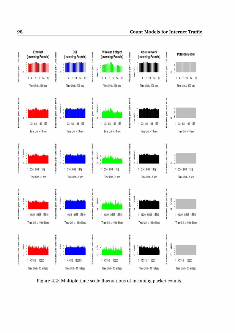
98 Count Models for Internet Traffic
Figure 4.2: Multiple time scale fluctuations of incoming packet counts.

4.2 Time aggregation of Internet Traffic Counts 99
Figure 4.3: Multiple time scale fluctuations of outgoing flow counts.

100 Count Models for Internet Traffic
Figure 4.4: Multiple time scale fluctuations of incoming flow counts.

4.2 Time aggregation of Internet Traffic Counts 101
Figure 4.5: Multiple time scale fluctuations of session counts.

102 Count Models for Internet Traffic
4.3 Count Models based on Self-Similarity
Self-similar count models have been developed to account for the strength of temporal
correlations in Internet traffic. In this category the most commonly used count models are
fractional Brownian motion (FBM), fractional Gaussian noise (FGN), fractional autoregres-
sive integrated moving average (FARIMA) and a count model based on superposition of the
heavy-tailed ON/OFF traffic sources.
4.3.1 Fractional Brownian Motion
A Gaussian process is a natural choice for modelling count data if one is interested in
second-order properties [Norros, 1995]. This is due to the central limit theorem; see [Addie,
1998], for example. For modelling variations in Internet traffic, fractional Brownian motion
(FBM) is a commonly used model for capturing strong correlations in data. It was first
formulated by [Kolmogorov, 1940] in his study about “spirals of Wiener”. Further statistical
properties of this model were developed in [Mandelbrot & Ness, 1968]. The FBM process
BH(t) is defined as
BH(t) =1
Γ(H + 1/2)
[ ∫ 0
−∞(|t− τ|H−1/2−|τ|H−1/2)dB(τ)+
∫ t
0|t− τ|H−1/2dB(τ)
], t ∈ R.
(4.1)
where H is the Hurst parameter, BH(0) = 0. For H = 1/2, we get B1/2(t) = B(t), which is
the distribution of Brownian motion. Therefore, FBM can be regarded as a generalization
of Brownian motion.
The covariance function of FBM, RBH , is given by
RBH(s, t) = Cov(BH(s), BH(t)) =VH
2(|s|2H + |t|2H − |t− s|2H), s, t ∈ R, (4.2)
where,
VH = var[BH(1)] =−Γ(2− 2H) cos(πH)
πH(2H − 1). (4.3)

4.3 Count Models based on Self-Similarity 103
It is clear from the covariance structure of BH that its increments are stationary and
self-similar; that is for a > 0 and t0 ∈ R,
BH(t0 + aτ)− BH(t0)d= aHBH(τ); τ ∈ R, (4.4)
where d= refers to the equality of finite dimensional distributions. This means that BH(t) has
the same distribution in all time scales [Barton & Poor, 1988]. Hence, BH(t) is a self-similar
process.
Internet traffic is inherently connectionless, that is, it is based on Internet Protocol’s best
effort delivery service. For such traffic, [Norros, 1995] proposed a normalized FBM with
Hurst parameter H ∈ [1/2, 1) which is denoted by Zt. Normalized FBM (Zt) plays an
important role in modelling fluctuations in accumulated traffic A(t), that is, amount of
traffic (bytes or packets) accumulated till time t. The cumulative traffic A(t) is given
as
A(t) = mt +√
amZt, (4.5)
where m > 0 is the mean input rate and a is the variance coefficient.
FBM (BH(t)) is characterized by the following features:
1. BH(t) has stationary increments.
2. The increment process is Fractional Gaussian Noise (FGN) which is dependent and
correlated except for the Hurst parameter value of 0.5.
3. BH(t) has continuous paths, that is , no jumps are allowed.
4. The finite dimensional marginal distributions of BH(t) are Gaussian.
Normalized FBM (Zt) has the following additional features:
1. Z0 = 0, and E[Zt] = 0 for all t.
2. E[Zt]2 = |t|2H for all t.
In [Norros, 1995] a notion of free traffic has been developed. It is defined as a traffic facing
unlimited network resources or arriving at an uncongested link. Accordingly, a general
model for free traffic aggregated from a large number of independent traffic sources is
FBM. Several studies reported that the LAN traffic at byte and packet count levels shows a

104 Count Models for Internet Traffic
dependence structure (power law decay of autocorrelation function) close to that of FBM
with Hurst parameter values higher than 0.5; see [Erramilli et al., 1996b; Taqqu et al., 1997;
Willinger et al., 1997], for example.
4.3.2 Fractional Gaussian Noise
The increment process of Brownian motion is white Gaussian noise. Similarly, the increment
process of fractional Brownian motion is a stationary sequence , known as fractional
Gaussian noise (FGN). Fractional Gaussian noise Yk is defined as
Yk = BH(k + 1)− BH(k), k ∈ I, (4.6)
where BH(.) is the FBM process defined in Equation 4.1. FGN is a second-order stationary
process with zero mean, and its variance E[Yj2] = E[BH(1)] = σ0
2 can be derived from
FBM. The autocovariance function r(k) of FGN is given as
r(k) =σ0
2
2[|k + 1|2H − 2|k|2H + |k− 1|2H]. (4.7)
For the Hurst parameter value H = 1/2, the FGN sequence reduces to white Gaussian noise.
Realizations of FGN exhibit long-range dependence for 1/2 < H 6 1. This can be observed
by the asymptotic behaviour of its autocovariance function, as k→ ∞ in
r(k) = σ02H(2H − 1)k2H−2. (4.8)
Hence, the autocovariance function of FGN has a power-law form and is non-summable.
This shows that FGN exhibits long-range dependence for 1/2 < H 6 1.
4.3.3 Fractional ARIMA Processes
Autoregressive models define the next random variable in a time series as a function of
previous values [Frost & Melamed, 1994]. Examples of such models are moving average
(MA), autoregressive moving average (ARMA) and autoregressive integrated moving av-
erage (ARIMA). An advantage of the ARIMA family of models is that they are applicable

4.3 Count Models based on Self-Similarity 105
in time series modelling. That is, unlike fractional Gaussian noise processes, the models
based on ARIMA processes can be combined in a natural way with various established
Box-Jenkins time series models [Leland et al., 1994]; for Box-Jenkin models, see [Box et al.,2013].
It should be noted that fractional Gaussian noise is a strictly second order self-similar
process with specification of autocovariance at all lags. Internet traffic can be LRD, but
it can also exhibit short-range correlations at small lags. Therefore, FGN is not flexible
enough to capture both short-range dependence and long-range dependence in Internet
traffic [Taqqu, 2003]. In [Hosking, 1981], a need for a family of models with the following
properties was recognized:
• explicit characterization of long-range dependence;
• flexibility to model both short-range and long-range dependence in data;
• ability to generate synthetic data from the model.
In [Hosking, 1981], the ARIMA model has been generalized to introduce a family of models
called fractional ARIMA (p, d, q) processes which meet the above requirements. In case of
fractional ARIMA (FARIMA) processes, the level of differencing d is allowed to take any real
value rather than being restricted to integer values. For the range 0 < d ≤ 1/2, FARIMA
processes exhibit long-range dependence.
The FARIMA (p, d, q) model is defined as
φ(B)4dXn = Θ(B)εn, (4.9)
where Xn is the fractional differenced random variable, εn is an independent and identically
distributed normal random variable having zero mean and variance σε2. The polynomials φ
and Θ are of order p and q, and are given as
φ(B) = 1− ϕ1B− · · · − ϕpBp,
Θ(B) = 1 + θ1B + · · ·+ θqBq,(4.10)
in terms of the backward shift operator B, defined as B(Xn) = Xn−1. These polynomials
control the short-range dependence in Xn. The fractional differencing operator is 4d =
106 Count Models for Internet Traffic
(1− B)d, given as
4d = (1− B)d =∞
∑j=0
Γ(j + d)Γ(d)Γ(j + 1)
. (4.11)
If 0 < d ≤ 1/2, the FARIMA process exhibits long-range dependence with Hurst parame-
ter
H = d +12
. (4.12)
It should be noted that the explicit formulae for the autocovariance function of general
FARIMA processes are rather complicated ([Hosking, 1981]). In a simple case, FARIMA
(0, d, 0) behaves like a fractional noise with autocovariance function r(k) given by
r(k) = σε2 (−1)kΓ(1− 2d)
Γ(k− d + 1)Γ(1− k− d). (4.13)
Though FARIMA models can capture long-range and short-range dependence in Internet
traffic, it requires several iterative steps to generate a series which can match the statistical
properties of an actual traffic trace; see the steps mentioned in [Liu et al., 1999], for
example.
4.3.4 Superposition of Heavy-tailed ON/OFF Sources
Fractional Brownian motion, its increment process Fractional Gaussian noise and FARIMA
models do capture the observed long-range dependence in Internet traffic, but they lack
any physical justification. In other words, these are models for aggregate traffic only
with no account for statistical behaviour of individual traffic sources. Internet traffic is a
superposition of traffic streams from various users and links. Therefore, a self-similar count
model is needed which, besides modelling aggregate traffic, also assumes a user-oriented
statistical behaviour of traffic sources.
In [Taqqu et al., 1997], a self-similar count model has been developed which is based
on the superposition of traffic sources having heavy-tailed ON and OFF periods of data
transmission. This superposition model converges asymptotically to a rescaled form of
fractional Brownian motion.

4.3 Count Models based on Self-Similarity 107
The following theorem is due to [Taqqu et al., 1997]:
Theorem 6 Assume m traffic sources having heavy-tailed ON and OFF periods with tail indicesα1, α2 and mean values µ1, µ2, respectively. Let m→ ∞ (vertical aggregation), and then timet→ ∞ (horizontal aggregation), then the aggregate cumulative packet count process A(Tt)behaves statistically like
A(Tt)→ Tmµ1
µ1 + µ2t︸ ︷︷ ︸
traffic mean level
+ TH√
L(T)mσlimBH(t).︸ ︷︷ ︸fluctuations around traffic mean level
(4.14)
Where T is a time rescaling factor, H is the Hurst parameter and BH(t) is an FBM process.
For an estimation procedure for L(T) and σlim, see [Taqqu et al., 1997].
Taqqu’s theorem further states that the Hurst parameter of the converged FBM process is
given as
H =3− α
2, (4.15)
where α is the minimum of tail indices of ON and OFF periods. The practical observability of
the above relation in Internet traffic has been discussed in [Abry et al., 2010a] and [Loiseau
et al., 2010]. It was found that though the heavy-tail index and the Hurst parameter depend
on each other, the relationship predicted by Equation 4.15 is not practically observable in
current Internet traffic. Therefore, this relation should not be used as quantitative estimator
of LRD parameters from heavy-tail index of traffic streams.
In [Taqqu et al., 1997], it has been shown that, if the order of limits in the theorem is
reversed, then the converged process is a Stable Levy Motion. That is, if time t → ∞(horizontal aggregation) and then m → ∞ (vertical aggregation), then the aggregate
cumulative packet count process A(Tt) behaves statistically like a Stable Levy Motion.
The theorem by [Taqqu et al., 1997] has been extended by [Kaj, 1999] for superposition of
m renewal processes with heavy-tailed interarrival time distributions in the range 1 < α ≤ 2,
and a similar FBM approximation has been proposed, though with a different scaling and
centring.

108 Count Models for Internet Traffic
4.4 Count Models based on Renewal Processes
The connection between a count model and its timing process (that is, interarrival time
distribution) is an important tool for researchers who are faced with the analysis of both
count data and interarrival time data. Using such a relationship, a researcher can develop
a model based on one form (counting or timing) and using its parameters, statistical
characteristics of the data in the other form can be reported. For example, a model for
interarrival time data can be established and from it predictions can be made about the
number of arrivals in a certain time interval. It is remarkable to note that over the years
thousands of count models have been developed; see [Wimmer & Altmann, 1999] for a
detailed description of various count models based on discrete univariate distributions. But
the connection between a count model and its timing process (interarrival time distribution)
has been addressed by very few [McShane et al., 2008].
The objective of this section is to describe properties of count models having a corresponding
timing process which can be used to capture statistical characteristics of Internet traffic
count data at fine time scales. Different count models assign a different probability mass
to integer values, representing traffic counts, in the body and tail part of a distribution.
A counting dataset can be equi-, over- or underdispersed depending on its variance to
mean relation. There are various count models which have been formulated to account
for a variety of dispersion in count data. Internet traffic at packet, flow and session level
is mostly overdispersed but under certain conditions (at sub-millisecond time scales, for
example) it can display equidispersion or even underdispersion (variance-mean curves to
assess dispersion can be seen in the next Chapter in Section 5.2.2). Below, we describe
some of the selected count data models (along with their associated timing processes)
which can be used in modelling Internet traffic count data.
4.4.1 Poisson Count Model
The Poisson distribution with its intensity parameter λ > 0 is a probability measure which
assigns a probability mass of e−λλk/(k!) to integers k ∈ N. In other words, the Poisson
count model is a model for increments, in time interval t, in which increments are assigned
probabilities according to a Poisson distribution. If N(t) denotes the number of counts in

4.4 Count Models based on Renewal Processes 109
the interval (0, t], then the Poisson count model is given by
P[N(t) = k] =e−λt(λt)k
k!, k = 0, 1, 2, . . . , λ > 0. (4.16)
The time durations between the successive Poisson events, that is interarrival times, follow
an exponential distribution with probability density fucntion fT given as
fT(t) = λe−λt, t > 0. (4.17)
The Poisson count model exhibits a constant hazard rate. This model is also known for its
memoryless property. The distribution of counts and corresponding interarrival times are
independent of the choice of origin (starting time). The mean of the number of events,
E[N(t)], in a unit interval of time, and the mean of duration between successive arrivals,
E[T], is given by
E[N(t)] = λ,
E[T] =1λ
.
The Poisson count model has the following features:
• The Poisson count model generates stationary counts with no trends, that is, event
probabilities do not change with time.
• The Poisson count model implies an exponential distribution for the underlying
interarrival process and the cumulative interarrival process can be represented by the
Erlang distribution.
• The counts resulting from the Poisson count model are independent or uncorrelated.
• The counts resulting from the Poisson count model are equidispersed, that is, the
variance of counts is equal to their mean.
According to [Cameron & Trivedi, 1996], the Poisson count model, though a benchmark
model for count data, may not be an appropriate model for count data always. For example,
in case of dependence between events, the probability of an arrival of event can increase
the likelihood of further arrivals. Also, the Poisson count model over-predicts the number
110 Count Models for Internet Traffic
of zero and under-predicts the number of non-zero counts away from the mean.
Nevertheless, the Poisson count model has been found to be useful in modelling the Internet
backbone packet level traffic due to the high degree of traffic multiplexing [Cao et al.,2003]. The applicability of the Poisson count model in Internet traffic and further theorems
has been discussed in Sections 2.6.2 and 3.3.
The Poisson process can be tailored to make its intensity a function dependent on time.
The resulting process is non-stationary and is called a time-dependent Poisson process
or doubly stochastic Poisson process. In Internet traffic count data, the intensity varies
from time to time. Therefore, for modelling Internet traffic, this non-stationary process is
better than a Poisson process with constant intensity. Nevertheless it should be noted that
describing a point process in terms of its intensity function obscures the discrete nature of
the arrival process [Lam, 1997]. An interesting alternative to the doubly stochastic Poisson
process is a renewal process based on the heavy-tailed Weibull interarrival times [Yannaros,
1994]; see also Sections 4.4.3 and 4.6 for relevant theory and Internet traffic count data
modelling.
4.4.2 Negative Binomial Count Model
The Poisson count model assigns significantly low probabilities to the values far away
from the mean. Moreover, the Poisson count data is always equidispersed. To overcome
these limitations a negative binomial count model can be used [Lawless, 1987]. If the rate
parameter λ of the Poisson count model is not constant and distributed according to the
Gamma distribution, then the resulting distribution of counts will be negative binomial.
In other words, the negative binomial count model is based on interarrival times being
exponentially distributed having rate parameter following a Gamma distribution.
Besides the classical parametrization of the negative binomial distribution, a mean specified
parametrization is more useful here, which can be written as
P(N = k) =Γ(k + d)k!Γ(d)
(µ
µ + d
)k(1
1 + µd−1
)d
, k = 0, 1, 2, ..., (4.18)
where µ is the mean and d > 0 is the dispersion parameter which controls the variance to
mean relation of the data produced by the negative binomial count model. The variance of
count model is Var(N) = µ + µ2/d. As d→∞, the variance of the data tends to become

4.4 Count Models based on Renewal Processes 111
equal to its mean, that is, Var(N)→µ so that the resulting distribution ultimately becomes
Poisson. For 0 < d < ∞, the variance of the data will exceed its mean µ. Thus, for the
dispersion values in the range 0 < d < ∞, the negative binomial distribution produces
overdispersed count data. It should be noted that the negative binomial distribution cannot
produce underdispersed data (variance less than mean) for any value of the dispersion
parameter d.
In summary, negative binomial count model has the following features:
1. The model allows arrival dependence based on positive contagion, that is, an arrival
(non-arrival) of an event increases (decreases) the probability of the next arrival.
2. The model can handle overdispersed data.
3. The model allows likelihood ratio and other standard maximum likelihood tests to be
implemented.
4. The convolution of the negative binomial random variables with the same overdis-
persion is also negative binomial, irrespective of the mean of the component random
variables (see page 459 in [Wilkinson, 1956]). The analytical form of the convolution
of negative binomial random variables has been derived in [Furman, 2007].
According to [Cameron & Trivedi, 1996], an alternate derivation of negative binomial
distribution assumes the underlying process to be non-stationary in the sense that an arrival
of an event increases the probability of further arrivals.
In the case of count data modelling, it is a sound practice to to evaluate the performance
of both the Poisson and negative binomial count models [Cameron & Trivedi, 1996]. We
have shown in Section 4.6 that negative binomial count model assigns appropriately high
probabilities to higher quantiles of Internet traffic count data. Assigning high probabilities to
higher quantiles or traffic counts in the tail region is important in Internet traffic modelling
because this regime affects network performance.
4.4.3 Weibull Count Model
The cumulative distribution function of a Weibull random variable X, representing interar-
rival times, can be written as
FX(x) = 1− e−λxc, x > 0, c > 0, (4.19)

112 Count Models for Internet Traffic
where c is the shape parameter and λ is the rate parameter. The probability density function
of the Weibull distribution is given as
fX(x) = λcxc−1e−λxc, x > 0, c > 0. (4.20)
The hazard rate of Weibull distribution admits a closed form expression as follows:
h(t) =f (t)
1− F(t)= λctc−1. (4.21)
The hazard rate of the Weibull distribution can be a constant, increasing or a decreasing
function of time based on the value of the shape parameter c. Therefore, Weibull distributed
interarrival times can generate equidispersed (for c = 1), underdispersed (for c > 1) and
overdispersed (for c < 1) count data.
In [Cameron & Trivedi, 1996], it has been emphasized that a count model is needed which
is dual to the continuous Weibull distribution. Such a count model can accommodate data
with time varying intensity. Considering such a requirement, a count model corresponding
to Weibull interarrival times has been formulated in [McShane et al., 2008]. It offers
a similar conceptual elegance and mathematical usefulness to that of the exponential-
Poisson connection. The model is applicable for all possible values of shape parameter
and can model counts resulting from heavy-tailed and non-heavy-tailed Weibull distributed
interarrival times.
If N(t) denotes the number of arrivals in time interval (0, t] with interarrival times being
Weibull distributed, then the Weibull count model is given as
P[N(t) = n] =∞
∑j=n
(−1)j+n(λtc)jαnj
Γ(cj + 1), n = 0, 1, 2, . . . , (4.22)
with
α0j = Γ(cj + 1)/Γ(j + 1), j = 0, 1, 2, . . . ,
αn+1j =
j−1
∑m=n
αnmΓ(cj− cm + 1)/Γ(j−m + 1),
where n = 0, 1, 2, . . .; j = n + 1, n + 2, n + 3, . . .; c is the Weibull shape parameter and λ

4.4 Count Models based on Renewal Processes 113
is the rate parameter. Although the number of terms in Equation 4.22 is infinite, due to
Taylor series expansion, a finite number of terms between 5 to 20 are sufficient for a good
approximation. We have truncated the series after 90 terms so as to obtain more accurate
results.
The Weibull count model has been derived by noting that an n-fold convolution of an
interarrival time distribution with itself gives the probability of time to the nth arrival.
Subtracting this probability (the n-fold convolution) with (n+1)-fold convolution of the
same interarrival time distribution gives the count model, that is, the probability of n counts
in time t. According to [McShane et al., 2008], the model is based on the use of Taylor series
expansion as there is no simple way to obtain a convolution of two or more continuous
Weibull random variables.
[McShane et al., 2008] has outlined the following features of the Weibull count model:
1. The model allows overdispersed, equidispersed and underdispersed count data.
2. The model is directly connected to the continuous time Weibull distribution for all
values of the shape parameter.
3. The model is computationally better than the iterative algorithms to calculate proba-
bility of counts resulting from the Weibull interarrival times; see [Rinne, 2008], for
such algorithms.
It is important to note that computation of the probabilities using Weibull count model
requires operations on gamma function, that involves factorials. Any attempt to use raw
factorials can lead to numerical instabilities. In order to overcome this issue, we recommend
to use log-gamma function and to calculate the gamma function using,
Γ(z) = eln Γ(z), (4.23)
where ln Γ(z) denotes the log-gamma function, a good approximation of which is given by
[Rocktaeschel, 1922], as
ln Γ(z) ≈(z− 1
2)
ln z− z +12
ln(2π). (4.24)
Some more approximations for log-gamma function can be found in [Espinosa & Moll,
2004].

114 Count Models for Internet Traffic
Additionally, using recurrence relation for the gamma function can be often very useful for
performance optimization of the count model, that is,
Γ(z + 1) = zΓ(z). (4.25)
The Weibull distribution has also an event prediction feature within a fixed sample size of
data. Assume that interarrival times between events follow the Weibull distribution and the
total number of events is N. The prediction of the number of arrivals N f in a future time
interval (tc, tw), provided that Nc (out of N) arrivals occurred by the time tc, is given as
([Nelson, 2000])
N f = N × q (4.26)
where q is given as
q =
[1− Nc
N
]−[
1− Nc
N
]( twtc )
α
(4.27)
The bounds on precision of the Weibull in-sample prediction estimator can be seen in
[Nordman & Meeker, 2002].
Our data analysis in this chapter is based on real Internet traffic from different networks.
The intensity in our traces vary from time to time as can be seen in Figures 4.1 to 4.5. Our
results in Section 4.6 shows that the Weibull count model can be regarded as a simple
counterpart of any non-Gaussian traffic model which can assign high probabilities to higher
quantiles at fine time scales. We have reported that a renewal process based heavy-tailed
Weibull interarrival times has a great potential in modelling packet, flow and session counts
in different networks.

4.4 Count Models based on Renewal Processes 115
4.4.4 Gamma Count Model
If interarrival times X follow the Gamma distribution, then their probability density function
can be written as
f (x; α, β) =βα
Γ(α)xα−1e−βx, x > 0, α > 0, β > 0, (4.28)
where α is the shape parameter and β is the scale parameter of the Gamma distribu-
tion.
It should be noted that the hazard rate function of the Gamma distribution cannot be
expressed in a closed form. According to [Winkelmann, 1995], the hazard rate function of
the Gamma distribution satisfies the following relation:
1h(t)
=∫ ∞
0e−βu(1 +
ut)α−1du. (4.29)
It follows from the above relation that the hazard rate h(t) of the Gamma distribution is
monotonically increasing for α > 1, decreasing for α < 1, and remains constant for α = 1.
Thus, the Gamma distributed interarrival times can generate underdispersed, overdispersed
and equidispersed count data.
In [Winkelmann, 1995], an expression for the probability of counts, in an interval of time t,denoted as N(t), when the interarrival times follow the Gamma distribution, is formulated
as
P[N(t) = n] = e−βtα−1
∑i=0
(βt)αn+i
(αn + i)!, n = 0, 1, 2, . . . . (4.30)
For α = 1, the Gamma count model reduces to the Poisson count model. For α > 1, the
model displays underdispersion, and for α < 1, the model results in overdispersed count
data [Winkelmann, 1995]. It should be noted that no closed form expression for the
Gamma count model is available for non-integer α. Therefore, for non-integer α, numerical
evaluation of the integral (which replaces the summation in Equation 4.30) is required.
This has performance implications for using this count model for modelling Internet traffic
count data which are mostly overdispersed (as can be observed from variance-mean curves
in Section 5.2.2).

116 Count Models for Internet Traffic
4.4.5 Mittag-Leffler Count Model
Another possible distribution, which displays overdispersion and equidispersion, is Mittag-
Leffler distribution. This distribution falls under the domain of attraction of stable laws
[Jose & Abraham, 2011].
The cumulative distribution function of a random variable X, representing interarrival
times, drawn from the Mittag-Leffler distribution is given as
F(x; α, k) =∞
∑k=1
(−1)k−1xkα
Γ(1 + kα), x > 0, 0 < α 6 1, (4.31)
and its probability density function is given by
f (x; α, k) =∞
∑k=1
(−1)k−1kαxkα−1
Γ(1 + kα), x > 0, 0 < α 6 1, (4.32)
where α is the shape parameter of this distribution.
The hazard rate of the Mittag-Leffler distribution can be written as
h(t) =∑∞
k=1
[(−1)k−1kαxkα−1
Γ(1+kα)
]∑∞
k=0
[(−1)k−1xkα
Γ(1+kα)
].
(4.33)
In [Jose & Abraham, 2011], an expression for probability of the counts, in an interval of
time (0, t] denoted as N(t), resulting from interarrival times based on the Mittag-Leffler
distribution, is formulated as
P[N(t) = n] =∞
∑j=1
[( j
n)(−1)j−ntjα
Γ(1 + jα)
], n = 0, 1, 2, . . . . (4.34)
According to [Jose & Abraham, 2011], the Mittag-Leffler count model has the following
properties:
• Poisson count model results as a special case for α = 1.
• All moments of Mittag-Leffler count model are finite for any α.

4.4 Count Models based on Renewal Processes 117
• For the range 0 < α < 1, the hazard rate of Mittag-Leffler count model is a decreasing
function of time. Therefore, the distribution exhibits negative duration dependence
which causes overdispersion in the count data.
4.4.6 Selecting Renewal Count Models for Internet Traffic
In Chapter 3, we have considered the analytical and goodness of fit capabilities of expo-
nential, Weibull and log-normal distributions for modelling interarrival times of packets,
flows and sessions. The heavy-tailed Weibull distributions were found to provide a best fit
to their interarrival time distributions, as well as they displayed an overall better queueing
performance at packet level.
Various types of arrival dependence and duration dependence1 can cause equi-dispersion,
over-dispersion and under-dispersion in count data. Internet traffic at packet, flow and
session count levels can have both arrival dependence and duration dependence. Therefore,
we need count models which can display all the three types of dispersion in the Internet
traffic count data.
On the basis of our discussion of count models and the interarrival time models, we now
present a joint analysis for selecting appropriate renewal count models.
• The cumulative distribution function of log-normal distribution is not defined in a
closed form expression. This implies that a count model corresponding to log-normal
distributed interarrival times cannot be derived in a closed form. The probability of
such counts cannot be evaluated without an algorithm based on numerical solution.
This has performance implications for modelling Internet traffic count data.
• The Poisson, Weibull count models have hazard rate in a closed form expression. On
the contrary, the hazard rate of the Gamma and Mittag-Leffler count models cannot
be expressed in closed form.
• The Gamma count model has no closed form expression of hazard rate for the case of
negative duration dependence (overdispersion). In this case, a numerical evaluation
of integral is required. This has performance implications for modelling Internet
traffic count data.
• Negative binomial count model can display over- and equidispersion. This model has
1See Section 2.3 for the description of the phenomena of arrival dependence and duration dependence.

118 Count Models for Internet Traffic
underlying interarrival times being exponentially distributed with Gamma distributed
rate parameter. It cannot exhibit underdispersion. Nevertheless, the negative binomial
count model offers a large range of overdispersed count data. Therefore, it can be
useful in modelling overdispersed count data of Internet traffic.
• The Weibull distributed interarrival times offers all the three types of dispersion in
the resulting count data, and the distribution has a formulation for its count model
[McShane et al., 2008].
In a backbone core network, Internet traffic tends to Poisson due to the increased level
of multiplexing [Cao et al., 2003]. Whereas, the traffic in access networks exhibits non-
Poisson features. The Weibull distribution has analytical justification because it is a limiting
distribution for interarrival times resulting from superposition of heavy-tailed streams
[Mitov & Yanev, 2006]. It also offers the best goodness of fit capabilities for packet, flow
and session interarrival times and an overall better queueing performance (as can be seen
in the previous Chapter).
Based on the above discussion and results in Chapter 3, we have selected the Poisson,
Weibull and negative binomial count models as candidate models for Internet traffic count
data modelling in our analysis of traffic at packet, flow and session levels in access and ISP
core networks.
4.5 Self-Similar Count Models versus Renewal Count Mod-
els
In this section, we present a critique on the applicability of count models based on self-
similar processes and renewal processes for Internet traffic count data modelling.
4.5.1 Applicability of Self-Similar Count Models
Taking into account the scope of research presented in this thesis, we outline the issues
concerning the applicability of self-similar count models in Internet traffic as follows:
• The FGN model allows the possibility of negative values which is not realistic in
modelling of packet or byte counts unless the mean of data is significantly greater
than its standard deviation [Norros, 1995].
4.5 Self-Similar Count Models versus Renewal Count Models 119
• Regarding the convergence to a pure Gaussian process under superposition, the
following remark is noteworthy. Namely, a distribution with heavy tail index greater
than two, that is, α > 2, even with a million convolutions of it with itself it will
eventually behave like Gaussian up to around three standard deviations but will retain
the heavy-tailed attributes outside of such a regime [Taleb, 2009] .
• The fractal properties introduced by the FGN process degenerate. The computational
efficiency of FGN for traffic generation decreases as the value of the Hurst parameter
increases to one [Riedi et al., 1999].
• The heavy tailed ON/OFF superposition models, leading to FBM in the limit, are
accurate only in the regime of coarser time scales, and they do not account for actual
queueing and multiplexing occurring in a network at fine time scales [Riedi et al.,1999].
• The FBM model abandons the classical framework of point arrival processes in favour
of modelling the “net” work or cumulative input process. That is, instead of defining
packet arrival times, FBM models the cumulative traffic arriving up to a certain
defined time instant. Therefore, the superposition models using FBM or FGN as a
limit counting process cannot be used in studies of the converged stochastic behaviour
of interarrival times [Gordon, 1996].
• The FBM and Gaussian processes can be expressed in discrete or continuous time.
The sampling rate required in a discrete time Gaussian model makes it quite different
from the corresponding continuous time Gaussian model [Addie, 1999]. For the
correlated interarrival times (of packets, flows or sessions), continuous time Gaussian
models are inappropriate due to fast tail decay. For discrete time Gaussian models,
there is a trade off in the choice of sampling interval. Long sampling intervals ensures
that discrete values (for example, packet counts per unit sampling interval) are not
negative but are not suitable for performance evaluation at the time scales concerning
traffic queueing or switching, and vice versa.
• Although the phenomena of burstiness and LRD are complementary to each other,
they in fact are different. A LRD process may or may not be bursty at fine time scales
[Tian et al., 2002]. Therefore, care should be taken in using self-similar count models
if one wants to generate bursty traffic data only.
• Traffic modelling based on self-similar count models should also specify an appro-
priate estimator for the degree of self-similarity. This is necessary because different

120 Count Models for Internet Traffic
estimators of Hurst parameter can provide different and even conflicting estimates for
the strength of self-similarity in traffic count data [Rea et al., 2013].
• The sudden changes in mean levels of count data can also cause LRD estimators to
provides false positives regarding strength of long-range dependence [Beran et al.,2013a]. Therefore, data should be carefully assessed with the help of appropriate
qualitative estimators of LRD (for example, the wavelet based estimator proposed in
[Abry et al., 1998]) to confirm the presence of self-similarity, and therefore, to justify
the applicability of self-similar count models.
• In [Addie et al., 1999], it has been shown that fitting the mean, variance and Hurst
parameter is not sufficient to consistently characterize Internet traffic count data
which exhibits long-range dependence. A fourth parameter defining the level of
aggregation is also required. This affects the parsimony of self-similar count models.
• Autoregressive models like FARIMA can capture the empirical second-order corre-
lations in data, but they do not generally fit the empirical marginal distribution of
traffic count data [Frost & Melamed, 1994].
4.5.2 Applicability of Renewal Count Models
Here, we outline some of the advantages which the renewal process framework offers if
one uses them in modelling Internet traffic count data.
• A traffic modelling framework has strong physical meanings if it is based on point
processes [Veitch et al., 2005]. Such a modelling framework can account for various
statistical characteristics of Internet traffic in a consistent manner. Renewal processes
can play an important role in establishing such a modelling framework. The self-
similar count modelling framework suffers from detection and estimation issues
regarding the strength of self-similarity. On the other hand, a traffic modelling
framework based on renewal processes has consistent methodologies to assess renewal
behaviour of traffic data and how much it deviates from it; see Section 2.2.
• Long-range dependence can be physically justified as the result of superposition of
renewal processes with heavy-tailed interarrival times, which in turn can be physically
justified by the access patterns of users. The superposition of such renewal processes
can generate long-range dependence or induce strong temporal correlations in the
superposed count process [Beran et al., 2013a].

4.5 Self-Similar Count Models versus Renewal Count Models 121
• Non-renewal processes can be approximated by appropriate renewal processes by
fitting a few lower order moments [Kuehn, 1979; Whitt, 1982].
• Point process based analysis offers a unified framework for modelling of the different
structural components of Internet traffic at packet, flow and session levels [Arfeen
et al., 2013].
• Count models based on various renewal processes can generate different types of
dispersion in count data. This is useful in modelling Internet traffic count data under
various load conditions. For example, renewal processes based on Weibull interarrival
times can generate underdispersed, equidispersed and overdispersed data, depending
on the value of the Weibull shape parameter.
• A renewal process based on heavy-tailed Weibull interarrival times has similar sta-
tistical properties as those of doubly stochastic Poisson processes or Cox processes
(Poisson processes with stochastic intensity) which is suitable for modelling variations
in Internet traffic count data [Yannaros, 1994].
• Renewal processes have also been used to develop switched Poisson processes with
time varying rates and dependencies between interarrival times. These models are
shown to exhibit a similar long-range dependence behaviour as that of Internet traffic.
They include Markov-modulated Poisson process (MMPP) and Pareto-modulated
Poisson process (PMPP); see [Fischer & Meier-Hellstern, 1993; Muscariello et al.,2005] and [Le-Ngoc & Subramanian, 2000], for example. These models are multi-state
and highly parametrized to fit properly to Internet traffic [Mallor et al., 2007]. Pure
renewal processes with heavy-tailed interarrival times provide a simple alternative to
such models.
• Renewal processes can be considered as a generalization of ON/OFF processes where
each ON period consists of one event (packet, flow or session). In such a case,
they are known as singular renewal processes in [Erramilli et al., 1996a]. Hence,
theorems regarding superposition of ON/OFF processes can also be generalized to
assess properties of superposition of pure renewal processes under relevant conditions;
see [Gaigalas & Kaj, 2003; Kaj, 1999], for example.
• Renewal processes can also be aggregated to implement approximate self-similar
processes with normal marginal distribution. An example of such a method is based
on spatial renewal process (SRP) which is a mixture of two independent renewal
processes with one of them having desired marginal distribution of traffic [Taralp

122 Count Models for Internet Traffic
et al., 1998].
4.6 Modelling Counts in Access and ISP Core Networks
As noted earlier, self-similar count models are applicable at coarse time scales. These time
scales are not relevant for network performance evaluation at switching or queueing levels.
For network performance evaluation we need traffic models which can model Internet
traffic at fine time scales (for example, micro or millisecond time scales). Such models are
required to produce interarrival time or count data having similar statistical characteristics
as that of Internet traffic, so that these models can also be used in simulations.
In this section, we compare the probability mass of traffic counts observed in access and
ISP core networks at fine time scales with the probability mass assigned by Poisson, Weibull
and negative binomial count models. Our experimental data set is the same as that used in
Chapter 3 and has been described in Section 1.7.
Here we describe the configuration of the count model plots in Figures 4.6, 4.7, 4.8 and
4.9. The rate parameters for Poisson, Weibull and negative binomial count models are
evaluated by applying maximum likelihood methods on traffic count data. Based on our
data analysis, we select dispersion parameter, d = 10, for the negative binomial count
model as it provides a good approximation to the traffic count data. The shape parameters
for the Weibull count models should ideally have exactly the same values for traffic counts
as that of the corresponding interarrival time data shown in Table 3.6. But due to truncation
of the infinite Taylor series in the Weibull count model, the values of the shape parameter
in Table 3.6 do not always provide an optimal fit to the corresponding count data. Based
on our analysis, we have observed that for the traffic count data, in general, lower values of
Weibull shape parameters, than those shown in Table 3.6, provide a better approximation to
the count data for all quantiles. The Weibull shape parameters for count data are shown in
Table 4.1. It can also be observed from Table 4.1 and Table 3.6 that the differences between
shape parameter of corresponding counts and interarrival times decreases as traffic moves
from access to ISP core network.
The plots in Figures 4.6, 4.7, 4.8 and 4.9 allow a comparative analysis of various count
models for session, flow and packet counts in case of Ethernet, DSL, Wireless hotspot
networks and their ISP core network. The tail region (higher quantiles) in each plot
has been shown separately in a sub-plot. The Weibull count model with value of shape

4.6 Modelling Counts in Access and ISP Core Networks 123
Table 4.1: Weibull shape parameter of packet, flow and session traffic counts
Weibull shape parameter (counts)
Access networks Sessions Outgoing flows Incoming flows Outgoing packets Incoming packets
Ethernet 0.5 0.8 0.8 0.5 0.5DSL 0.5 0.6 0.81 0.8 0.5Wireless hotspot 0.3 0.5 0.5 0.6 0.5
ISP core network 0.8 0.8 0.8 0.5 0.6
parameters less than one, as summarized in Table 4.1, assigns more probability mass to
the count values in the tail region. Compared with the empirical probability mass of traffic
counts (sessions, flows and packets), it can be observed that the Weibull count model has
much better performance than Poisson and negative binomial count models. In the body
part of the traffic count data distribution (lower values), Poisson and negative binomial
count models provide better fits, but they cannot capture the probability mass of the higher
count values in the tail part of Internet traffic count data distribution at packet, flow and
session levels. On the other hand, the Weibull count model performs best in the tail part
and assigns higher probability mass to the higher quantiles. The negative binomial count
model is better than Poisson count model and can be considered as a close competitor of the
Weibull count model. This is due to the fact that the underlying interarrival times of negative
binomial counts are exponential with rate parameter being Gamma distributed.
Due to the ever increasing number of users and application mixture, it is expected that
a large part of probability mass in traffic count data distribution will shift more towards
the tail side. Therefore, the count models which can assign appropriately large probability
mass to higher quantiles at fine time scales can play an important role in modelling future
Internet traffic at packet, flow and session levels.
In case of the Ethernet, DSL and ISP core networks, one can see from the plots in Figures
4.6, 4.7 and 4.9 that the Weibull count model provides a very good fit to the higher values
of counts in the tail part of our count data distribution. The counts in the tail parts can have
a significant impact on the network performance at fine time scales. The Figure 4.8 shows
that in the case of a Wireless hotspot network, the Weibull count model provides a better fit
to count data in both body and tail parts of the count data distribution as compared with
the Poisson and negative binomial count models.
Also it can also be observed from Table 4.1 that, in general, the Weibull shape parameter for
counts of sessions, flows and packets increases as traffic moves from various access networks

124 Count Models for Internet Traffic
to the ISP core network. This implies that, in general, the strength of overdispersion
decreases as traffic moves from access to ISP core network (that is, increased multiplexing).
Exceptions are also possible as can be seen in the case of outgoing packet counts. Here, the
shape parameter of packet counts in ISP core network is less than the shape parameter of
the components. This means that it is also possible that the strength of overdispersion can
increase due to the increased multiplexing of traffic.
Similar to Table 3.6, Table 4.1 shows that the Weibull shape parameter for the counts of
structural components of Internet traffic in Wireless hotspot network has comparatively
smaller values as compared to Ethernet and DSL networks. As noted in the previous chapter
concerning interarrival time models, we restate the need for more traffic analysis from other
Wireless hotspot networks to establish if the lower values of the Weibull shape parameter
can act as a signature for traffic in Wireless hotspot networks.
1 2 3 4 5 6 7 8 9 11 13 15 17 19 21 23 27 32 34 56
Ethernet network (Sessions)
Session counts (10ms)
Pro
babi
lity
0.00
0.05
0.10
0.15
0.20
0.25
16 18 20 22 24 31 33 42
0.00
000
0.00
010
0.00
020
Session counts in Ethernet networkPoisson count model (λ = 2.01)Weibull count model (c = 0.5, λ = 2.01)Negative binomial count model (d = 10, µ = 2.01)
(a)
Figure 4.6: Counts in Ethernet network.

4.6 Modelling Counts in Access and ISP Core Networks 125
13
57
911
1315
1719
2123
2527
2931
3335
3739
4143
4547
4951
5355
5759
6163
6669
74
Ethe
rnet
net
work
(Out
goin
g flo
ws)
Outgo
ing flo
w co
unts
(10m
s)
Probability
0.000.050.100.15
1619
2225
2831
3437
4043
4649
5255
5861
6469
0.0000.0010.0020.0030.0040.005
Outgo
ing flo
w co
unts
in Et
hern
et ne
twor
kPo
isson
coun
t mod
el (λ
=5.24
)W
eibull
coun
t mod
el (c
=0.8,
λ=5
.24)
Nega
tive b
inomi
al co
unt m
odel
(d=1
0, µ=
5.24)
(b)
Figure 4.6: Counts in Ethernet network (Continued).

126 Count Models for Internet Traffic
13
57
911
1315
1719
2123
2528
3033
3739
4251
5759
6367
6975
7991
105109
168
Ethernet network (Incoming flows)
Incoming flow counts (10ms)
Probability
0.00 0.05 0.10 0.15 0.20
1720
2326
3035
3946
5762
6770
79104
1090e+00 4e−05 8e−05
Incoming flow counts in Ethernet networkPoisson count model (λ=3.4)W
eibull count model (c=0.8, λ=3.4)Negative binomial count model (d=10, µ=3.4)
(c)
Figure 4.6: Counts in Ethernet network (Continued).

4.6 Modelling Counts in Access and ISP Core Networks 127
1 2 3 4 5 6 7 8 9 10 11 12 13 14 15 16 17 18 19 20 21 22 23 24 25 26 27 29 30 31 34 35 38
Ethernet network (Outgoing packets)
Outgoing packet counts (100µs)
Pro
ba
bility
0.0
00
.05
0.1
00
.15
0.2
00
.25
0.3
0
15 16 17 18 19 20 21 22 23 24 25 26 27 29 30 31 34 35 38
0e
+0
01
e−
05
2e
−0
53
e−
05
4e
−0
5
Outgoing packet counts in Ethernet networkPoisson count model (λ = 1.54)Weibull count model (c = 0.5, λ = 1.54)Negative binomial count model (d = 10, µ = 1.54)
(d)
Figure 4.6: Counts in Ethernet network (Continued).

128 Count Models for Internet Traffic
13
57
911
1315
1719
2123
2527
2931
3335
3739
4143
4547
4951
5355
57
Ethernet network (Incoming packets)
Incoming packet counts (100µs)
Probability
0.00 0.05 0.10 0.15 0.20 0.25
1719
2123
2527
2931
3335
3739
4143
4547
4951
5355
570e+00 1e−04 2e−04 3e−04 4e−04
Incoming packet counts in Ethernet networkPoisson count model (λ=2.26)W
eibull count model (c=0.5, λ=2.26)Negative binomial count model (d=10, µ=2.26)
(e)
Figure 4.6: Counts in Ethernet network (Continued).

4.6 Modelling Counts in Access and ISP Core Networks 129
1 2 3 4 5 6 7 8 9 10 11 12 13 14 15 16 17 18 19 21
DSL network (Sessions)
Session counts (10ms)
Pro
ba
bili
ty
0.0
00
.05
0.1
00
.15
0.2
00
.25
0.3
0
10 11 12 13 14 15 16 17 18 19 21
0.0
00
00
.00
10
0.0
02
00
.00
30
Session counts in DSL networkPoisson count model (λ = 1.6)Weibull count model (c = 0.5, λ = 1.6)Negative binomial count model (d = 10, µ = 1.6)
(a)
1 2 3 4 5 6 7 8 9 10 11 12 13 14 15 16 17 18 19 20 21 22 23
DSL network (Outgoing flows)
Outgoing flow counts (10ms)
Pro
ba
bili
ty
0.0
00
.05
0.1
00
.15
0.2
00
.25
16 17 18 19 20 21 22 23
0.0
00
00
0.0
00
10
0.0
00
20
0.0
00
30 Outgoing flow counts in DSL network
Poisson count model (λ = 2.5)Weibull count model (c = 0.6, λ = 2.5)Negative binomial count model (d = 10, µ = 2.5)
(b)
Figure 4.7: Counts in DSL network.

130 Count Models for Internet Traffic
1 2 3 4 5 6 7 8 9 10 11 12 13 14 15 16 17 18 20 21
DSL network (Incoming flows)
Incoming flow counts (10ms)
Pro
ba
bili
ty
0.0
00
.05
0.1
00
.15
0.2
00
.25
0.3
00
.35
8 9 10 11 12 13 14 15 16 17 18 20 21
0e
+0
01
e−
04
2e
−0
43
e−
04
Incoming flow counts in DSL networkPoisson count model (λ = 0.81)Weibull count model (c = 0.5, λ = 0.81)Negative binomial count model (d = 10, µ = 0.81)
(c)
1 2 3 4 5 6 7 8 9 10 11 12 13 14
DSL network (Outgoing packets)
Outgoing packet counts (100µs)
Pro
ba
bili
ty
0.0
00
.05
0.1
00
.15
0.2
00
.25
0.3
00
.35
5 6 7 8 9 10 11 12 13 14
0.0
00
0.0
02
0.0
04
Outgoing packet counts in DSL networkPoisson count model (λ = 0.83)Weibull count model (c = 0.8, λ = 0.83)Negative binomial count model (d = 10, µ = 0.83)
(d)
Figure 4.7: Counts in DSL network (Continued).

4.6 Modelling Counts in Access and ISP Core Networks 131
1 2 3 4 5 6 7 8 9 10 11 12 13 14 15 16 17 18 19 20 21 22 23 24
DSL network (Incoming packets)
Incoming packet counts (100µs)
Pro
ba
bili
ty
0.0
00
.05
0.1
00
.15
0.2
00
.25
0.3
00
.35
15 16 17 18 19 20 21 22 23 24
0e
+0
02
e−
06
4e
−0
66
e−
06
8e
−0
6
Incoming packet counts in DSL networkPoisson count model (λ = 1.24)Weibull count model (c = 0.5, λ = 1.24)Negative binomial count model (d = 10, µ = 1.24)
(e)
Figure 4.7: Counts in DSL network (Continued).
1 2 3 4 5 6 7 8 9 10 11 12 13 14 15 16 18 26 29 30
Wireless hotspot network (Sessions)
Session counts (10ms)
Pro
ba
bili
ty
0.0
00
.05
0.1
00
.15
0.2
0
5 6 7 8 9 10 12 14 16 26 30
0.0
00
00
.00
10
0.0
02
0
Session counts in Wireless hotspot networkPoisson count model (λ = 0.33)Weibull count model (c = 0.3, λ = 0.33)Negative binomial count model (d = 10, µ = 0.33)
(a)
Figure 4.8: Counts in Wireless hotspot network.

132 Count Models for Internet Traffic
1 2 3 4 5 6 7 8 9 11 13 15 17 19 21 23 25 27 32 54
Wireless hotspot network (Outgoing flows)
Outgoing flow counts (10ms)
Pro
ba
bili
ty
0.0
00
.05
0.1
00
.15
0.2
00
.25
0.3
0
5 7 9 11 13 15 17 19 21 23 25 27 32 54
0.0
00
0.0
02
0.0
04
Outgoing flow counts in Wireless hotspot networkPoisson count model (λ = 0.51)Weibull count model (c = 0.5, λ = 0.51)Negative binomial count model (d = 10, µ = 0.51)
(b)
1 2 3 4 5 6 7 8 9 10
Wireless hotspot network (Incoming flows)
Incoming flow counts (10ms)
Pro
ba
bili
ty
0.0
00
.02
0.0
40
.06
0.0
80
.10
0.1
2
8 9 10
0e
+0
04
e−
06
8e
−0
6
Incoming flow counts in Wireless hotspot networkPoisson count model (λ = 0.15)Weibull count model (c = 0.5, λ = 0.15)Negative binomial count model (d = 10, µ = 0.15)
(c)
Figure 4.8: Counts in Wireless hotspot network (Continued).

4.6 Modelling Counts in Access and ISP Core Networks 133
1 2 3 4 5 6 7 8 9 10 12 14 16 18 20 22 24 27
Wireless hotspot network (Outgoing packets)
Outgoing packet counts (100µs)
Pro
ba
bili
ty
0.0
00
.05
0.1
00
.15
3 5 7 9 11 13 15 17 19 21 23 26
0.0
00
0.0
01
0.0
02
0.0
03
0.0
04
Outgoing packet counts in Wireless hotspot networkPoisson count model (λ = 0.22)Weibull count model (c = 0.6, λ = 0.22)Negative binomial count model (d = 10, µ = 0.22)
(d)
1 2 3 4 5 6 7 8 9 10 11 12 13 14 15 16 17 18 19 20 21 22
Wireless hotspot network (Incoming packets)
Incoming packet counts (100µs)
Pro
ba
bili
ty
0.0
00
.05
0.1
00
.15
0.2
0
4 5 6 7 8 9 11 13 15 17 19 21
0.0
00
0.0
01
0.0
02
0.0
03
0.0
04 Incoming packet counts in Wireless hotspot network
Poisson count model (λ = 0.32)Weibull count model (c = 0.5, λ = 0.32)Negative binomial count model (d = 10, µ = 0.32)
(e)
Figure 4.8: Counts in Wireless hotspot network (Continued).

134 Count Models for Internet Traffic
1 3 5 7 9 11 13 15 17 19 21 23 25 28 31 33 37 46
ISP core network (Sessions)
Session counts (10ms)
Pro
ba
bili
ty
0.0
00
.05
0.1
00
.15
16 18 20 22 24 26 29 32 34 43 57
0e
+0
02
e−
04
4e
−0
46
e−
04
8e
−0
4
Session counts in ISP core networkPoisson count model (λ = 3.93)Weibull count model (c = 0.8, λ = 3.93)Negative binomial count model (d = 10, µ = 3.93)
(a)
Figure 4.9: Counts in ISP core network.

4.6 Modelling Counts in Access and ISP Core Networks 135
13
57
911
1315
1719
2123
2527
2931
3335
3739
4143
4547
4951
5355
5759
6163
6567
7072
74
ISP
core
net
work
(Out
goin
g flo
ws)
Outgo
ing flo
w co
unts
(10m
s)
Probability
0.000.020.040.060.080.100.12
2629
3235
3841
4447
5053
5659
6265
6872
78
0.00000.00040.00080.0012
Outgo
ing flo
w co
unts
in IS
P co
re ne
twor
kPo
isson
coun
t mod
el (λ
=8.25
)W
eibull
coun
t mod
el (c
=0.8,
λ=8
.25)
Nega
tive b
inomi
al co
unt m
odel
(d=1
0, µ=
8.25)
(b)
Figure 4.9: Counts in ISP core network (Continued).

136 Count Models for Internet Traffic
13
57
911
1315
1719
2123
2527
2931
3335
3941
4955
5863
6670
7681
91104
109
ISP core network (Incoming flows)
Incoming flow counts (10ms)
Probability
0.00 0.05 0.10 0.15
1720
2326
2932
3540
4956
6369
7684
104109
0e+00 2e−04 4e−04
Incoming flow counts in ISP core networkPoisson count model (λ=4.36)W
eibull count model (c=0.8, λ=4.36)Negative binomial count model (d=10, µ=4.36)
(c)
Figure 4.9: Counts in ISP core network (Continued).

4.6 Modelling Counts in Access and ISP Core Networks 137
1 2 3 4 5 6 7 8 9 10 11 12 13 14 15 16 17 18 19 20 21 22 23 24 25 26 27 28 29 30 31 32 35 38 41
ISP core network (Outgoing packets)
Outgoing packet counts (100µs)
Pro
ba
bility
0.0
00
.05
0.1
00
.15
0.2
00
.25
25 26 27 28 29 30 31 32 35 38 41
0.0
e+
00
4.0
e−
06
8.0
e−
06
1.2
e−
05 Outgoing packet counts in ISP core network
Poisson count model (λ = 2.58)Weibull count model (c = 0.5, λ = 2.58)Negative binomial count model (d = 10, µ = 2.58)
(d)
Figure 4.9: Counts in ISP core network (Continued).

138 Count Models for Internet Traffic
13
57
911
1315
1719
2123
2527
2931
3335
3739
4143
4547
4951
5355
5759
62
ISP core network (Incoming packets)
Incoming packet counts (100µs)
Probability
0.00 0.05 0.10 0.15 0.20
2527
2931
3335
3739
4143
4547
4951
5355
5759
620e+00 4e−05 8e−05
Incoming packet counts in ISP core networkPoisson count model (λ=3.83)W
eibull count model (c=0.6, λ=3.83)Negative binomial count model (d=10, µ=3.83)
(e)
Figure 4.9: Counts in ISP core network (Continued).

4.6 Modelling Counts in Access and ISP Core Networks 139
4.6.1 Assessing Probability Mass for Higher Quantiles
Here we present a comparative analysis regarding the sum of the probability mass of higher
quantiles of the traffic count data and that of the probability mass assigned to the same
quantiles by Poisson, Weibull and negative binomial count models. For every access and
ISP core networks under consideration, Table 4.2 shows the sum of the probability mass
of session count quantiles, denoted as C0.25, which are greater than the 0.25 quantiles
of session count data. The sum of the probability mass assigned by count models to the
same quantiles, denoted as P0.25, is shown in the following columns. It can be seen that
the sum of the probability mass assigned by the Weibull count model is closest to the
sum of probability mass of session count data in every network. Negative binomial and
Poisson count models assign relatively low probability masses to higher quantiles. Similar
observation can be made from Tables 4.3, 4.4, 4.5 and 4.6 regarding outgoing flow counts,
incoming flow counts, outgoing packet counts and incoming packet counts, respectively.
As higher quantiles of count data affect network performance, therefore, we recommend
to use the Weibull count model as it assigns larger probability mass to higher quantiles as
well as appropriate probability mass to quantiles in the body part of the traffic count data
distribution.
The Weibull count model with shape parameter less than one gives irregular and overdis-
persed counts, so we recommend its use in Internet traffic modelling. Varying the shape
parameter in the range 0 to 1 gives a variety of statistical irregularity (burstiness) and
overdispersion and this flexibility enables the Weibull count model to perform better in
modelling counts of various structural components of Internet traffic (packets, flows and
sessions) at fine time scales. Also, the Weibull distribution has an in-sample prediction
feature which can be used for a limited traffic forecasting. The Weibull count model can also
be easily used in computer simulations of various access, ISP and backbone core networks to
generate traffic loads similar to real Internet traffic at packet, flow and session levels.

140 Count Models for Internet Traffic
Table4.2:
Probabilitym
ass:session
countsversus
countm
odels
Sumofprobability
mass
forcounts
greaterthan
0.25quantile
Closeness
metric
(Model/C
ounts)C
losenessm
etric(A
bsoluteError)
C0.25
P0.25
R=
P0.25 /
C0.25
E=|P
0.25 −C
0.25 |
Access
network
sessionW
eibullN
eg.binom
.Poisson
Weibull
Neg.
binom.
PoissonW
eibullN
eg.binom
.Poisson
countscount
model
countm
odelcount
model
countm
odelcount
model
countm
odelcount
model
countm
odelcount
model
Ethernet0.00082
0.0016.27×
10 −7
4.038×10 −
9121.95%
0.08%0.00%
0.0001800.000819373
0.000819996
DSL
0.005790.01261
0.000274.59×
10 −5
217.79%4.66%
0.79%0.006820
0.0055200000.0057441
Wireless
hotspot0.01052
0.003880.00056
0.0003636.88%
5.32%3.42%
0.0066400.009960000
0.01016
ISPcore
network
0.003940.00184
0.000481.65×
10 −5
46.70%12.18%
0.42%0.002100
0.0034600000.0039235

4.6 Modelling Counts in Access and ISP Core Networks 141
Tabl
e4.
3:Pr
obab
ility
mas
s:ou
tgoi
ngflo
wco
unts
vers
usco
unt
mod
els
Sum
ofpr
obab
ility
mas
sfo
rco
unts
grea
ter
than
0.25
quan
tile
Clo
sene
ssm
etri
c(M
odel
/Cou
nts)
Clo
sene
ssm
etri
c(A
bsol
ute
Erro
r)C
0.25
P 0.2
5R=
P 0.2
5/C
0.25
E=|P
0.25−
C0.
25|
Acc
ess
netw
ork
Out
goin
gflo
wW
eibu
llN
eg.
bino
m.
Pois
son
Wei
bull
Neg
.bi
nom
.Po
isso
nW
eibu
llN
eg.
bino
m.
Pois
son
coun
tsco
unt
mod
elco
unt
mod
elco
unt
mod
elco
unt
mod
elco
unt
mod
elco
unt
mod
elco
unt
mod
elco
unt
mod
elco
unt
mod
el
Ethe
rnet
0.02
197
0.02
030
0.00
452
0.00
036
92.4
0%20
.57%
1.64
%0.
0016
70.
0174
5000
0.02
1610
0
DSL
0.00
092
0.00
136
6.58×
10−
66.
81×
10−
814
7.83
%0.
72%
0.01
%0.
0004
40.
0009
1342
0.00
0919
9
Wir
eles
sho
tspo
t0.
0234
70.
0109
50.
0028
30.
0019
246
.66%
12.0
6%8.
18%
0.01
252
0.02
0640
000.
0215
500
ISP
core
netw
ork
0.00
583
0.00
606
0.00
076
1.99×
10−
610
3.95
%13
.04%
0.03
%0.
0002
30.
0050
7000
0.00
5828
0

142 Count Models for Internet Traffic
Table4.4:
Probabilitym
ass:incom
ingflow
countsversus
countm
odels
Sumofprobability
mass
forcounts
greaterthan
0.25quantile
Closeness
metric
(Model/C
ounts)C
losenessm
etric(A
bsoluteError)
C0.25
P0.25
R=
P0.25 /
C0.25
E=|P
0.25 −C
0.25 |
Access
network
Incoming
flowW
eibullN
eg.binom
.Poisson
Weibull
Neg.
binom.
PoissonW
eibullN
eg.binom
.Poisson
countscount
model
countm
odelcount
model
countm
odelcount
model
countm
odelcount
model
countm
odelcount
model
Ethernet0.00081
0.000175.27×
10 −5
6.39×10 −
720.99%
6.51%0.08%
0.0006400.000757300
0.0008093610
DSL
0.001360.00177
8.03×10 −
52.17×
10 −5
130.15%5.90%
1.60%0.000410
0.0012797000.0013383000
Wireless
hotspot5.55×
10 −5
4.63×10 −
81.38×
10 −9
2.62×10 −
100.08%
0.00%0.00%
0.0000550.00005549
0.0000554997
ISPcore
network
0.001360.00215
0.000521.37×
10 −5
158.09%38.24%
1.01%0.000790
0.0008400000.0013463000

4.6 Modelling Counts in Access and ISP Core Networks 143
Tabl
e4.
5:Pr
obab
ility
mas
s:ou
tgoi
ngpa
cket
coun
tsve
rsus
coun
tm
odel
s
Sum
ofpr
obab
ility
mas
sfo
rco
unts
grea
ter
than
0.25
quan
tile
Clo
sene
ssm
etri
c(M
odel
/Cou
nts)
Clo
sene
ssm
etri
c(A
bsol
ute
Erro
r)C
0.25
P 0.2
5R=
P 0.2
5/C
0.25
E=|P
0.25−
C0.
25|
Acc
ess
netw
ork
Out
goin
gpa
cket
Wei
bull
Neg
.bi
nom
.Po
isso
nW
eibu
llN
eg.
bino
m.
Pois
son
Wei
bull
Neg
.bi
nom
.Po
isso
nco
unts
coun
tm
odel
coun
tm
odel
coun
tm
odel
coun
tm
odel
coun
tm
odel
coun
tm
odel
coun
tm
odel
coun
tm
odel
coun
tm
odel
Ethe
rnet
0.00
014
0.00
019
1.37×
10−
71.
12×
10−
913
5.71
%0.
10%
0.00
%0.
0000
5000
0.00
0139
8630
0.00
0139
9989
DSL
0.02
643
0.02
107
0.01
407
0.01
029
79.7
2%53
.23%
38.9
3%0.
0053
6000
0.01
2360
0000
0.01
6140
0000
Wir
eles
sho
tspo
t0.
0297
30.
0306
00.
0216
70.
0202
410
2.93
%72
.89%
68.0
8%0.
0008
7000
0.00
8060
0000
0.00
9490
0000
ISP
core
netw
ork
5.05×
10−
65.
37×
10−
51.
68×
10−
101.
05×
10−
1510
63.3
7%0.
00%
0.00
%0.
0000
4865
0.00
0005
0498
0.00
0005
0500

144 Count Models for Internet Traffic
Table4.6:
Probabilitym
ass:incom
ingpacket
countsversus
countm
odels
Sumofprobability
mass
forcounts
greaterthan
0.25quantile
Closeness
metric
(Model/C
ounts)C
losenessm
etric(A
bsoluteError)
C0.25
P0.25
R=
P0.25 /
C0.25
E=|P
0.25 −C
0.25 |
Access
network
Incoming
packetW
eibullN
eg.binom
.Poisson
Weibull
Neg.
binom.
PoissonW
eibullN
eg.binom
.Poisson
countscount
model
countm
odelcount
model
countm
odelcount
model
countm
odelcount
model
countm
odelcount
model
Ethernet0.00064
0.001746.65×
10 −7
2.69×10 −
9271.88%
0.10%0.00%
0.00110000.0006393350
0.0006399973
DSL
4.53×10 −
52.32×
10 −5
1.26×10 −
87.63×
10 −11
51.21%0.03%
0.00%0.0000221
0.00004528740.000452999
Wireless
hotspot0.02112
0.012790.00537
0.0043560.56%
25.43%20.60%
0.0083300.0157500000
0.0167700000
ISPcore
network
0.000190.00044
9.87×10 −
84.04×
10 −12
231.58%0.05%
0.00%0.0002500
0.00018990100.0001900000

4.7 Summary of the Chapter 145
4.6.2 Closeness Metrics
It is important to use statistical metrics in order to assess closeness of a given count model
to the count data of packets, flows and sessions. A simple metric can be defined as ratio of
the probability mass assigned to counts greater than 0.25 quantile to the corresponding
actual counts. If R denotes the ratio in percentage, P0.25 denotes sum of the probability
mass assigned by count model to counts greater than 0.25 quantile and C0.25 denotes the
corresponding sum of the probability mass for actual counts, then the closeness metric Rcan be defined as,
R =P0.25
C0.25. (4.35)
Here a ratio of R = 1.0 means a perfect match between the actual counts and the counts
resulting from proposed count model. R greater than 1.0 represents over-estimation whereas
R smaller than 1.0 represents under-estimation of the counts.
Another simple metric to assess the closeness is absolute error, denoted by E, and defined
as,
E = |P0.25 − C0.25|. (4.36)
Tables 4.2-4.6 show values of both closeness metrics for the corresponding count data
obtained from the access and ISP core networks under consideration. The ratio metric
has been presented in percentage. A perfect match of 100% is difficult to observe as we
are approximating non-renewal data with renewal models. However, one can see that the
Weibull count model offers a better approximation in 16 out of 20 cases considered.
4.7 Summary of the Chapter
An important step in understanding Internet traffic at packet, flow and session levels is to
assess its fluctuations at various increasing time scales. Such a qualitative multiple time
scale analysis is very helpful for selecting appropriate statistical analysis techniques and
models for traffic counts which can exhibit short-range or long-range dependencies.
Self-similar count models like FBM have been successfully applied in capturing long or short

146 Count Models for Internet Traffic
range dependence (scaling properties) of Internet traffic data at packet count level. Such
models are suitable for traffic modelling at coarse time scales. Internet traffic modelling
at fine time scales is a different scenario where strong correlations (if any) cannot fully
manifest themselves. Nevertheless, the Internet traffic count data at packet, flow and
session levels cannot be treated as entirely independent or having Poisson features at fine
time scales.
We have seen that based on arrival or duration dependence, various renewal processes
can generate a variety of dispersion in count data. Internet traffic at packet, flow and
session count levels is mostly overdispersed in access networks and tends to equidispersed
in backbone core networks. Moreover, under certain conditions (for example, low level
traffic aggregation) Internet traffic can also display underdispersion.
We have described the theoretical properties of various count models offering various
types of dispersion. These models include Poisson, negative binomial, Weibull, Gamma
and Mittag-Leffler count models. We conclude that among the models considered in this
study, the count model based on Weibull distributed interarrival times performs the best
in modelling Internet traffic counts at packet, flow and session level at fine time scales in
various access and ISP core networks.

Chapter 5
Scaling Models for Internet Traffic
“ Teletraffic is indeed a phenomenon of scales. Rarely do we find a quantity, ofany kind, spread across such a broad range. What is even more significantis that this range will continue to grow, with the inevitable improvements,closely following those of computing, in the bandwidth of connections andthe capacity of switches, and all this without any limit known to science.
”Darryl Veitch, 2009
5.1 Introduction
The term scale has different interpretations in various disciplines of science and engineering.
In Physics, it has been used as a standard reference to quantify measurements of the physical
quantities. In signal processing, the term scale can be used to refer to the serial correlation
lengths in data, for example. Scaling as a reference measure has been applied in terms of
time and space. Scaling in time means that properties of a system can be defined specific
to the observation time scale, which can change if the observation time scale changes.
Whereas, scaling in space means that properties of a system can be specified in terms of its
geometry. Two main objectives in time and space specific scaling analysis are (i) to study
system or process properties which are specific to various scales and (ii) to study transfer
mechanisms between scales. According to [Abry et al., 2010b], the concept of scaling or

148 Scaling Models for Internet Traffic
scale invariance is converse of the scaling concept as a reference measure of time or space.
That is, the behaviour of a system cannot be characterized by a single scale of time or space
only, and the observed phenomenon or the behaviour of a system depends on all relevant
time or space scales. According to [Abry et al., 2010b], this “non-property” (the effect of all
scales instead of a single or specific scale of time or space) is referred to as scaling law or
scaling behaviour, or in the teletraffic context, simply scaling. Accordingly, scaling can also
be regarded as a signature of strong organization based on the time or space invariance of
a certain key behaviour of a given system or process.
In Internet traffic modelling literature, the term scaling has been used interchangeably with
such terms as self-similarity, long-range dependence or fractals. Though, in a global sense
these terms can be regarded as synonymous, nevertheless, the distinction should be made
clear. Namely, the terms fractal and self-similarity have geometric origins, whereas the terms
scaling and long-range dependence refer to statistical properties. It is, in fact, the fractal
behaviour which makes a process or an object to appear self-similar over a range of scales
of time or space. In this thesis, we undertake a statistical definition of these terminologies.
To be more precise, a strictly second-order self-similar process is referred as mono-fractal
process or long-range dependent process. Scaling refers to the multiple time scale view
of strength of long-range dependence which can demarcate regions where LRD is weak or
strong with mono-fractal or multi-fractal behaviour. The latter means that there exists more
than one scaling exponents to characterize data.
In most of the literature concerning Internet traffic analysis and modelling, the term scalinghas been used in the global context, that is, a multiple time scale view of LRD in traffic
count data, to characterize it by a single scaling exponent, that is, Hurst parameter. The
scaling analysis can also be performed in a local context. The local scaling analysis helps in
identification of local irregularities in data. More specifically, it allows us to investigate the
presence of multi-fractal behaviour.
The main contributions of this chapter are:
• Investigating burstiness, global and local scaling behaviour of packet, flow and session
counts in access networks. The impact of traffic transformation under access to ISP
core network is also reported.
• Proposing suitable traffic models based on renewal processes which can capture
overall burstiness and the scaling profile of Internet traffic.

5.2 Burstiness in Internet Traffic 149
5.2 Burstiness in Internet Traffic
In the literature concerning Internet traffic modelling, the concept of burstiness has been
extensively used but rarely defined in an appropriate context because there is still no
standard definition of burstiness [Wischik, 2006]. According to [Gusella, 1991], mostly
the term burstiness has been invoked for data which shows more variability than a Poisson
process. It is true that a process having more variability than a Poisson process is bursty.
Nevertheless, in order to define burstiness and to avoid any vagueness surrounding it,
a characterization of variability is needed, at least in an appropriate context. It should
be noted that temporal structures in data affect variability, which cannot be captured
by simple indices like coefficient-of-variation and peak-to-average ratio of rates. In fact,
peak-to-average ratio of rates can be considered as a crude measure of burstiness, but it is
significantly dependent on the length of time interval used for rate measurement [Frost &
Melamed, 1994]. In [Gusella, 1991], it has been suggested to use the index of dispersion
for intervals (IDI) and index of dispersion for counts (IDC) for characterizing burstiness;
see Section 2.2 for the definition of these indices.
While characterizing Internet traffic as LRD, it is even more important to define burstiness.
This is necessary because, without an approximate definition of burstiness, some contra-
dictory interpretations regarding statistical behaviour of Internet traffic can emerge [Tian
et al., 2002]. Namely, one can find reports that the Internet traffic is long-range dependent
and bursty. However, there are also claims that it is showing near-Poisson and non-bursty
nature. See the difference between the findings reported in [Jiang & Dovrolis, 2005] and
[Cao et al., 2003]. The apparent dichotomy can be resolved if we do not equate the concept
of burstiness with long-range dependence. A long-range dependent time series or data can
appear either bursty or smooth at a given time scale. Therefore, the concept of burstiness is
about characterizing variability at a given time scale. As shown in [Tian et al., 2002], the
concept of burstiness and long-range dependence (or scaling) are complementary to each
other. In fact, the apparent contradictory conclusions of earlier works also complement
each other.
The measures of burstiness proposed by [Gusella, 1991] are indices of dispersion for
intervals and counts (IDI and IDC). We have presented the results of IDI analysis of Internet
traffic in Chapter 3. Here, we present our IDC analysis of Internet traffic belonging to access
and their ISP core networks. We have also presented a multiple time scale analysis based on
variance-mean method to assess burstiness. This method can be considered as a multiple

150 Scaling Models for Internet Traffic
time scale extension of the method in [Tian et al., 2002].
5.2.1 Burstiness: Index of Dispersion for Counts Analysis
As we have already mentioned, the indices of dispersion for intervals and counts (IDI and
IDC) can be used to characterize burstiness of Internet traffic arrival process. In this section,
we use IDC to characterize traffic burstiness as suggested by [Casale et al., 2012]. We assess
burstiness of packet, flow and session counts in access and ISP core networks.
The index of dispersion for counts (IDC), It, was defined by Equation 2.9 in Section 2.2. An
IDC curve can be interpreted as follows. Namely, an IDC curve which is horizontal and
equal to 1 for all t is the signature of a Poisson process. An IDC curve which is horizontal
above I(t) = 1 shows a behaviour which is renewal and signifies that the process has more
variability than a Poisson process. Also, fluctuations in an IDC curve can be regarded as a
qualitative measure of burstiness. These fluctuations are caused by nonstationarities like a
sudden change in the mean or variance of counts.
Figure 5.1 depicts the IDC curves for packet, flow and session counts in the Ethernet, DSL,
Wireless hotspot and their ISP core networks under investigation in this study. Interpreting
the plots horizontally allows to assess the multiplexing of traffic from access networks into
the ISP core network. By observing the fluctuations in the IDC curves, the traffic in Ethernet
and Wireless hotspot networks is found to be more bursty than the corresponding traffic
in the DSL network. Also, it can be observed that the average value of IDC for ISP core
network traffic is smaller than that for the access network traffic which has the highest
average value of the IDC. The same traffic multiplexing view of IDC curves (that is, having
read the plots in Figure 5.1 horizontally) shows that for a given structural component of
traffic (packet, flow or session), the fluctuations shown in the IDC curve for the ISP core
network traffic are smaller than in the traffic of the access network which shows the highest
IDC fluctuations. This leads us to a conclusion that the multiplexing or superposition of
traffic from the access networks reduces the burstiness of traffic in the ISP core network
under our investigation. Such a multiplexing gain is observed for the counts of all the
structural components of Internet traffic, that is, packets, flows and sessions.

5.2 Burstiness in Internet Traffic 151
Figure 5.1: Index of dispersion for counts (IDC) curves of traffic in Ethernet, DSL, Wirelesshotspot and ISP core networks.

152 Scaling Models for Internet Traffic
5.2.2 Burstiness: Variance-Mean Analysis
Burstiness can also be assessed in terms of the relation between the variance and mean,
that is, plotting variance versus mean of the counts in non-overlapping windows of fixed
size. If such a plot is linear, then this implies smooth traffic. If the variance-mean plot is
quadratic, then it implies bursty traffic [Tian et al., 2002]. The variance-mean relation can
also be used in implementing traffic management policies [Kawahara et al., 2013].
We extend the variance-mean analysis technique to assess this relation at multiple time
scales. Such a multiple time scale analysis of the variance-mean relation can be more
informative as it can partially reveal the presence of any correlations in data. It should be
emphasized that the presence of burstiness at multiple time scales can be indicative of the
presence of a scaling phenomenon. Nevertheless, any conclusion about presence of scaling
or its strength in data should not be entirely based on analysis of variance-mean relation at
single or multiple time scales. Relevant methodologies (such as discussed in Section 5.3)
should be applied to assess scaling, its onset or strength in data.
In this section, we analyse the variance-mean relation of traffic counts of packets, flows and
sessions belonging to the access network and ISP core networks under our consideration.
The lowest time scale is 100 microseconds and the highest time scale is 200 milliseconds
(that is, equal to a typical round trip time). The plots in Figures 5.2, 5.3 and 5.4 show the
variance-mean behaviour of packet, flow and session counts in the Ethernet, DSL, Wireless
hotspot networks and their ISP core network, under our investigation, at the aggregation
time scales of 100 microseconds, 10 milliseconds and 200 milliseconds, respectively. Each
figure reports the behaviour of variance-mean relation at a given time scale. The effect of
multiplexing or superposition of the traffic belonging to various access networks in the ISP
core network can be observed in the last column of these figures.
The following observations can be made from a multiple time scale investigation of the
variance-mean plots in these figures:
• The traffic multiplexing in the ISP core network at any time scale makes the variance-
mean relation appear more linear as compared to the variance-mean relation of traffic
in the access networks.
• The slope of variance-mean relation in the ISP core network is dominated by the
largest traffic contributor access network, that is, the Ethernet network.
• The variance-mean relations for the packets, flows and sessions (belonging to the

5.2 Burstiness in Internet Traffic 153
traffic traces under our consideration) appear to be linear at the fine time scales of
100 microseconds and 10 milliseconds, as shown in Figures 5.2 and 5.3. For 200
milliseconds aggregation time interval, the variance-mean relations deviate from
linearity, especially in the case of incoming and outgoing packet counts, as can be
seen in Figure 5.4. A plausible reason for this behaviour is that correlations are not
obvious at fine time scales, but they can manifest themselves at coarser time scales.
• The packet, flow and session counts appear to be over-dispersed in all networks for
all time scales. The amount of over-dispersion increases with increasing time scale for
traffic aggregation.

154 Scaling Models for Internet Traffic
0.00 0.02 0.04
0.0
00.0
4
T s = 100µs, segments size = 512 data points
Session CountsEthernet Network
Va
ria
nce
Mean
0.00 0.02 0.04 0.06
0.0
00.0
40.0
8
T s = 100µs, segments size = 512 data points
Session CountsDSL Network
Va
ria
nce
Mean
0.00 0.04 0.08 0.12
0.0
00.0
60.1
2
T s = 100µs, segments size = 512 data points
Session CountsWireless hotspot
Va
ria
nce
Mean
0.05 0.10 0.15
0.0
20.1
0
T s = 100µs, segments size = 512 data points
Session CountsISP Core Network
Va
ria
nce
Mean
0.05 0.15
0.0
50.1
5
T s = 100µs, segments size = 512 data points
Incoming flow counts
Va
ria
nce
Mean
0.00 0.02 0.04 0.06
0.0
00.0
6
T s = 100µs, segments size = 512 data points
Incoming flow counts
Va
ria
nce
Mean
0.000 0.010 0.020 0.030
0.0
00
0.0
20
T s = 100µs, segments size = 512 data points
Incoming flow counts
Va
ria
nce
Mean
0.05 0.15 0.25
0.0
50.2
5
T s = 100µs, segments size = 512 data points
Incoming flow counts
Va
ria
nce
Mean
0.05 0.15 0.25
0.1
0.3
T s = 100µs, segments size = 512 data points
Outgoing flow counts
Va
ria
nce
Mean
0.02 0.06 0.10
0.0
20.0
8
T s = 100µs, segments size = 512 data points
Outgoing flow counts
Va
ria
nce
Mean
0.00 0.04 0.08 0.12
0.0
00.0
8
T s = 100µs, segments size = 512 data points
Outgoing flow counts
Va
ria
nce
Mean
0.05 0.15 0.25
0.1
0.3
0.5
T s = 100µs, segments size = 512 data points
Outgoing flow counts
Va
ria
nce
Mean
2.0 2.5 3.0
48
12
T s = 100µs, segments size = 512 data points
Incoming packet counts
Va
ria
nce
Mean
0.8 1.2 1.6
1.5
2.5
T s = 100µs, segments size = 512 data points
Incoming packet counts
Va
ria
nce
Mean
0.2 0.3 0.4 0.5
0.2
0.8
1.4
T s = 100µs, segments size = 512 data points
Incoming packet counts
Va
ria
nce
Mean
3.0 3.5 4.0 4.5
48
12
T s = 100µs, segments size = 512 data points
Incoming packet counts
Va
ria
nce
Mean
1.2 1.4 1.6 1.8 2.0
1.5
2.5
3.5
T s = 100µs, segments size = 512 data points
Outgoing packet counts
Va
ria
nce
Mean
0.6 0.8 1.0 1.2
0.8
1.2
1.6
T s = 100µs, segments size = 512 data points
Outgoing packet counts
Va
ria
nce
Mean
0.15 0.25 0.35
0.2
0.6
1.0
T s = 100µs, segments size = 512 data points
Outgoing packet counts
Va
ria
nce
Mean
2.0 2.4 2.8
3.0
4.0
5.0
T s = 100µs, segments size = 512 data points
Outgoing packet counts
Va
ria
nce
Mean
Figure 5.2: Variance-mean plots for session, flow and packet counts in access and ISP corenetworks at 100 microseconds time aggregation.

5.2 Burstiness in Internet Traffic 155
1.5 2.0 2.5 3.0
26
10
14
T s = 10ms, segments size = 512 data points
Session CountsEthernet Network
Va
ria
nce
Mean
1.2 1.6 2.0
24
6
T s = 10ms, segments size = 512 data points
Session CountsDSL Network
Va
ria
nce
Mean
0.2 0.4 0.6 0.8
12
34
T s = 10ms, segments size = 512 data points
Session CountsWireless hotspot
Va
ria
nce
Mean
3.0 3.5 4.0 4.5 5.0
48
12
T s = 10ms, segments size = 512 data points
Session CountsISP Core Network
Va
ria
nce
Mean
3 4 5 6 7
0100
200
T s = 10ms, segments size = 512 data points
Incoming flow counts
Va
ria
nce
Mean
1.0 1.5 2.0 2.5
0.5
2.0
3.5
T s = 10ms, segments size = 512 data points
Incoming flow counts
Va
ria
nce
Mean
0.2 0.4 0.6 0.8 1.0
0.5
1.5
T s = 10ms, segments size = 512 data points
Incoming flow counts
Va
ria
nce
Mean
4 5 6 7 8
0100
200
T s = 10ms, segments size = 512 data points
Incoming flow counts
Va
ria
nce
Mean
4 5 6 7 8
10
25
T s = 10ms, segments size = 512 data points
Outgoing flow counts
Va
ria
nce
Mean
2.0 2.5 3.0 3.5 4.0
35
79
T s = 10ms, segments size = 512 data points
Outgoing flow counts
Va
ria
nce
Mean
0.2 0.4 0.6 0.8 1.0
04
812
T s = 10ms, segments size = 512 data points
Outgoing flow counts
Va
ria
nce
Mean
6 7 8 9 11 1310
25
40
T s = 10ms, segments size = 512 data points
Outgoing flow counts
Va
ria
nce
Mean
180 220 260
1000
4000
T s = 10ms, segments size = 512 data points
Incoming packet counts
Va
ria
nce
Mean
100 120 140
600
900
T s = 10ms, segments size = 512 data points
Incoming packet counts
Va
ria
nce
Mean
20 30 40 50 60
100
400
T s = 10ms, segments size = 512 data points
Incoming packet counts
Va
ria
nce
Mean
320 360 400 440
2000
5000
T s = 10ms, segments size = 512 data points
Incoming packet counts
Va
ria
nce
Mean
130 150 170
500
2000
T s = 10ms, segments size = 512 data points
Outgoing packet counts
Va
ria
nce
Mean
70 80 90 100
120
180
T s = 10ms, segments size = 512 data points
Outgoing packet counts
Va
ria
nce
Mean
15 20 25 30 35
50
150
T s = 10ms, segments size = 512 data points
Outgoing packet counts
Va
ria
nce
Mean
240 260 280
1000
3000
T s = 10ms, segments size = 512 data points
Outgoing packet counts
Va
ria
nce
Mean
Figure 5.3: Variance-mean plots for session, flow and packet counts in access and ISP corenetworks at 10 milliseconds time aggregation.

156 Scaling Models for Internet Traffic
38 40 42 44
100
160
T s = 200ms, segments size = 512 data points
Session CountsEthernet Network
Va
ria
nce
Mean
30 32 34 36
110
130
T s = 200ms, segments size = 512 data points
Session CountsDSL Network
Va
ria
nce
Mean
5.5 6.5 7.5
15
25
35
T s = 200ms, segments size = 512 data points
Session CountsWireless hotspot
Va
ria
nce
Mean
74 78 82
220
280
340
T s = 200ms, segments size = 512 data points
Session CountsISP Core Network
Va
ria
nce
Mean
65 70 75 80
01500
T s = 200ms, segments size = 512 data points
Incoming flow counts
Va
ria
nce
Mean
16 18 20 22 24
50
200
T s = 200ms, segments size = 512 data points
Incoming flow counts
Va
ria
nce
Mean
2.5 3.5 4.5
040
T s = 200ms, segments size = 512 data points
Incoming flow counts
Va
ria
nce
Mean
80 90 100 110
01500
T s = 200ms, segments size = 512 data points
Incoming flow counts
Va
ria
nce
Mean
95 105 115
600
800
T s = 200ms, segments size = 512 data points
Outgoing flow counts
Va
ria
nce
Mean
45 50 55
200
300
T s = 200ms, segments size = 512 data points
Outgoing flow counts
Va
ria
nce
Mean
8 9 10 11 12
30
50
70
T s = 200ms, segments size = 512 data points
Outgoing flow counts
Va
ria
nce
Mean
150 160 170 180
800
1100
T s = 200ms, segments size = 512 data points
Outgoing flow counts
Va
ria
nce
Mean
4200 4600 5000
100000
350000
T s = 200ms, segments size = 512 data points
Incoming packet counts
Va
ria
nce
Mean
2300 2450 2600
40000
70000
T s = 200ms, segments size = 512 data points
Incoming packet counts
Va
ria
nce
Mean
600 700 800
10000
30000
T s = 200ms, segments size = 512 data points
Incoming packet counts
Va
ria
nce
Mean
7200 7600 8000
200000
450000T s = 200ms, segments size = 512 data points
Incoming packet counts
Va
ria
nce
Mean
2900 3100 3300
50000
80000
T s = 200ms, segments size = 512 data points
Outgoing packet counts
Va
ria
nce
Mean
1600 1700
14000
22000
T s = 200ms, segments size = 512 data points
Outgoing packet counts
Va
ria
nce
Mean
380 420 460 500
4000
10000
T s = 200ms, segments size = 512 data points
Outgoing packet counts
Va
ria
nce
Mean
5000 5200 5400
70000
120000
T s = 200ms, segments size = 512 data points
Outgoing packet counts
Va
ria
nce
Mean
Figure 5.4: Variance-mean plots for session, flow and packet counts in access and ISP corenetworks at 200 milliseconds time aggregation.

5.2 Burstiness in Internet Traffic 157
5.2.3 Burstiness: Count Models
The variance-mean plots of the proposed count models, described in Chapter 4, have been
depicted in Figure 5.5. The Poisson count model generates data with variance equal to it’s
mean. Negative binomial count model exhibits overdispersion. The plots for the Weibull
count model show that, depending on the value of the shape parameter , it has the flexibility
to generate counts which can exhibit various types of variability and burstiness similar to
that exhibited by packet, flow and session counts in access and ISP core networks. The
burstiness profile of all count models shown in the figure matches with burstiness profile of
traffic data at fine time scales as shown in Figures 5.2 and 5.3. The Weibull count model
is more flexible than Poisson and negative binomial count models because it can generate
data with linear variance mean relation having both positive and negative slopes.
3.8 3.9 4.0 4.1 4.2
3.0
3.2
3.4
3.6
3.8
4.0
4.2 segments size = 512 data points
mean=4
Poisson Count Model
Varia
nce
Mean
3.8 3.9 4.0 4.1 4.2 4.3
4.0
4.5
5.0
segments size = 512 data points
mean=4, dispersion=10
Neg. Binom. Count Model
Varia
nce
Mean
2.2 2.4 2.6 2.8
6.0
7.0
8.0
9.0
segments size = 512 data points
mean=4, shape=0.3
Weibull Count Model
Varia
nce
Mean
6.0 6.2 6.4 6.6 6.8
8.5
9.0
9.5
10.0
11.0
segments size = 512 data points
mean=4, shape=0.5
Weibull Count Model
Varia
nce
Mean
Figure 5.5: A comparison of a sample variance-mean relation for various count models(“mean” denotes the rate parameter).

158 Scaling Models for Internet Traffic
5.3 Scaling in Internet Traffic
The concept of scaling is not directly related to burstiness at a given time scale [Wischik &
Ganesh, 2007]. Burstiness at multiple time scales can provide an indication of the presence
of scaling phenomenon. Nevertheless, it is essential to assess strength of any dependency
structure in data. The most important factor which can help in determining the presence
of scaling is the strength of autocorrelations in data at various lags. A slow decay of
autocorrelation function (ACF) shows the presence of scaling behaviour in data.
The autocorrelation function plots for our investigated traffic in access and ISP core networks
are shown in Figure 5.6 and 5.7. It should be noted that a slow decay of autocorrelation
functions (ACF) at a particular time scale can be used as evidence of the presence of strong
scaling or LRD (see Equations 2.13 and 2.14). A note of caution here is that a fast decay
of ACF at a particular time scale cannot be used as a justification for absence of scaling.
This is because data can be highly correlated at other time scales. Figure 5.6 shows that
ACF decays fast for session and flow counts at 10 milliseconds aggregation time interval,
implying short range dependence or absence of scaling. In the same figure, the ACF for
packet counts decays very slow, implying long-range dependence or presence of scaling.
The plots in Figure 5.7 show that if we estimate the ACF for the same traffic data at a
coarser time scale of 200 milliseconds, the ACF of session and flow counts decay slow which
implies onset of scaling. Therefore, ACF should be assessed at multiple time scales in order
to have an appropriate evidence of scaling in data.
The plots in Figures 5.6 and 5.7 also show that the superposition of the traffic from access
networks maintains the slow ACF decay in ISP core network traffic. It can be observed that
the autocorrelation function of traffic counts (packets, flows and sessions) in the ISP core
network is dominated by autocorrelations from the access network that contributes the
largest volume of traffic, that is, the Ethernet network.
Having seen that burstiness and slow ACF decay can be considered as an indication of
scaling or long-range dependence, provided that they are assessed at multiple time scales,
it should be noted that one can distinguish two types of scaling:
• Global scaling
• Local scaling
Global scaling means that a single scaling exponent or Hurst parameter is sufficient to
characterize the data at all time scales. Local scaling refers to the situations when a single

5.3 Scaling in Internet Traffic 159
scaling exponent cannot characterize the data at all time scales.
As we show in the next section, using the theory of wavelets, the phenomenon of global
and local scaling can be investigated in both a qualitative and a quantitative manner. This
theory allows for easier and more conclusive analysis than purely time domain analysis,
which we we have conducted so far.
0 200 600 1000
0.0
0.4
0.8
T s = 10ms
Session countsEthernet Network
Lag
AC
F
0 200 600 1000
0.0
0.4
0.8
T s = 10ms
Session countsDSL Network
Lag
AC
F
0 200 600 1000
0.0
0.4
0.8
T s = 10ms
Session countsWireless hotspot
LagA
CF
0 200 600 1000
0.0
0.4
0.8
T s = 10ms
Session countsISP Core Network
Lag
AC
F
0 200 600 1000
0.0
0.4
0.8
T s = 10ms
Incoming flow counts
Lag
AC
F
0 200 600 1000
0.0
0.4
0.8
T s = 10ms
Incoming flow counts
Lag
AC
F
0 200 600 1000
0.0
0.4
0.8
T s = 10ms
Incoming flow counts
Lag
AC
F
0 200 600 1000
0.0
0.4
0.8
T s = 10ms
Incoming flow counts
Lag
AC
F
0 200 600 1000
0.0
0.4
0.8
T s = 10ms
Outgoing flow counts
Lag
AC
F
0 200 600 1000
0.0
0.4
0.8
T s = 10ms
Outgoing flow counts
Lag
AC
F
0 200 600 1000
0.0
0.4
0.8
T s = 10ms
Outgoing flow counts
Lag
AC
F
0 200 600 1000
0.0
0.4
0.8
T s = 10ms
Outgoing flow counts
Lag
AC
F
0 200 600 1000
0.0
0.4
0.8
T s = 10ms
Incoming packet counts
Lag
AC
F
0 200 600 1000
0.0
0.4
0.8
T s = 10ms
Incoming packet counts
Lag
AC
F
0 200 600 1000
0.0
0.4
0.8
T s = 10ms
Incoming packet counts
Lag
AC
F
0 200 600 1000
0.0
0.4
0.8
T s = 10ms
Incoming packet counts
Lag
AC
F
0 200 600 1000
0.0
0.4
0.8
T s = 10ms
Outgoing packet counts
Lag
AC
F
0 200 600 1000
0.0
0.4
0.8
T s = 10ms
Outgoing packet counts
Lag
AC
F
0 200 600 1000
0.0
0.4
0.8
T s = 10ms
Outgoing packet counts
Lag
AC
F
0 200 600 1000
0.0
0.4
0.8
T s = 10ms
Outgoing packet counts
Lag
AC
F
Figure 5.6: Autocorrelation function (ACF) of traffic in Ethernet, DSL, Wireless hotspot andISP core network at 10 milliseconds time aggregation.

160 Scaling Models for Internet Traffic
0 200 600 1000
0.0
0.4
0.8
T s = 200ms
Session countsEthernet Network
Lag
AC
F
0 200 600 1000
0.0
0.4
0.8
T s = 200ms
Session countsDSL Network
Lag
AC
F
0 200 600 1000
0.0
0.4
0.8
T s = 200ms
Session countsWireless hotspot
Lag
AC
F
0 200 600 1000
0.0
0.4
0.8
T s = 200ms
Session countsISP Core Network
Lag
AC
F
0 200 600 1000
0.0
0.4
0.8
T s = 200ms
Incoming flow counts
Lag
AC
F
0 200 600 1000
0.0
0.4
0.8
T s = 200ms
Incoming flow counts
Lag
AC
F
0 200 600 1000
0.0
0.4
0.8
T s = 200ms
Incoming flow counts
Lag
AC
F
0 200 600 1000
0.0
0.4
0.8
T s = 200ms
Incoming flow counts
Lag
AC
F
0 200 600 1000
0.0
0.6
T s = 200ms
Outgoing flow counts
Lag
AC
F
0 200 600 1000
0.0
0.6
T s = 200ms
Outgoing flow counts
Lag
AC
F
0 200 600 1000
0.0
0.4
0.8
T s = 200ms
Outgoing flow counts
Lag
AC
F
0 200 600 1000
0.0
0.4
0.8
T s = 200ms
Outgoing flow counts
Lag
AC
F
0 200 600 1000
0.0
0.4
0.8
T s = 200ms
Incoming packet counts
Lag
AC
F
0 200 600 1000
0.0
0.4
0.8
T s = 200ms
Incoming packet counts
Lag
AC
F
0 200 600 1000
0.0
0.4
0.8
T s = 200ms
Incoming packet counts
Lag
AC
F
0 200 600 1000
0.0
0.4
0.8
T s = 200ms
Incoming packet counts
Lag
AC
F
0 200 600 1000
0.0
0.4
0.8
T s = 200ms
Outgoing packet counts
Lag
AC
F
0 200 600 1000
0.0
0.4
0.8
T s = 200ms
Outgoing packet counts
Lag
AC
F
0 200 600 1000
0.0
0.4
0.8
T s = 200ms
Outgoing packet counts
Lag
AC
F
0 200 600 1000
0.0
0.6
T s = 200ms
Outgoing packet counts
Lag
AC
F
Figure 5.7: Autocorrelation function (ACF) of traffic in Ethernet, DSL, Wireless hotspot andISP core network at 200 milliseconds time aggregation.

5.3 Scaling in Internet Traffic 161
5.3.1 Background on Global and Local Scaling
Global scaling is induced by long-range dependence (high temporal correlations) in traffic
counts in such a way that counts are strictly mono fractal (or deterministically self-similar).
This means that a single scaling exponent can characterize the strength of autocorrelations.
There are various quantitative estimators to evaluate strength of LRD using the Hurst pa-
rameter, such as Rescaled Range, Periodogram, Whittle’s and Aggregated-Variance methods.
Due to different procedures and assumptions for underlying data, these estimators produce
different estimates of Hurst parameter when applied to the same data [Karagiannis et al.,2006; Molnar & Dang, 2000; Rea et al., 2013; Ritke et al., 2001]. Hence, we adopt quali-
tative aspects of the wavelet-based estimator for our analysis regarding global and local
scaling. In fact, as compared with the other quantitative estimators of LRD, the wavelet
based global scaling analysis provides a multiple time scale view of long-range dependence
in a time series. This technique can quantify the global scaling exponent as well as it can be
used to demarcate time scales over which LRD strength is low, medium or high. Here, we
describe the wavelet based detection and estimation method for global scaling.
Global scaling can be investigated by a wavelet based multiresolution analysis technique
proposed in [Abry et al., 1998]. It is based on plotting wavelet energy as a function of
increasing time scales. The resulting plot is called Log-scale Diagram (LD) plot. This method
is non-parametric and based on the Discrete Wavelet transform (DWT). The wavelet basis
functions, such as Haar wavelets, possess scaling property themselves. Therefore, they
are suitable for the detection and estimation of scaling in data generated by the processes
having long memory or significant autocorrelations. The wavelet based global scaling
method measures the energy of time series at various fine and coarse time scales. The value
of this energy is a function of the variance of the wavelet coefficients at various time scales.
The method is described below.
Consider a time series, representing traffic counts, X(t) of length n. Let Ts be the reference
or sampling time scale (smallest time scale). For example, X(t) can be a series representing
the number of packets, flows or sessions recorded at a time granularity of Ts. The same
process X(t) can be viewed (in terms of wavelet coefficients) at increasingly coarser time
scales, that is, at Tj = 2jTs for j = 1, 2, . . . , Nj. Increasing values of j correspond to
increasing coarser time scales Tj, where Nj is the number of wavelet coefficients at octave
j = 1, ..., Nj = blog2(n)c. The octave j corresponds to the time scale 2jTs that defines the
width of time bin for the process X(t) viewed at octave j. Let 4tjk be the kth bin time
interval at scale j. Then4tjk consists of the intervals4tj−1
2k and4tj−12k+1. If X j
k is the amount

162 Scaling Models for Internet Traffic
of traffic in 4tjk, then X j
k = X j−12k + X j−1
2k+1. The Haar wavelet coefficients d(j, k) at scale jare defined as
d(j, k) =X j−1
2k − X j−12k+1
2j/2 , k = 1, ..., Nj. (5.1)
The square of wavelet coefficient, |d(j, k)|2, measures the amount of energy (function of
variance of wavelet coefficients) in the time series at the time instant 2jk. The magnitude of
energy at scale j increases with the variance of the wavelet coefficients at previous scale
j− 1. The energy function at octave j is defined as
(Energy)j =∑
Njk=1 d(j, k)2
Nj. (5.2)
The confidence intervals are derived from the variance of the energy based on Gaussian
assumption. The variance of the Energy is given as
var(log2(Energy)j) ∼2
Nj ln2 2. (5.3)
According to [Abry et al., 1998], the second order global scaling behaviour of a time series
is captured by the variation of log2(Energy) with j, which can be observed by plotting
log2(Energy) versus j. A straight line with positive slope gives an indication of scaling
behaviour between different time scales of width 2jk and 2j(k + 1). The presence of varying
slopes between different time scales provides a qualitative indication of the changing
strength of scaling. Here, an estimate for Hurst parameter (H), which can be calculated by
using weighted linear regression, is given as
H =12
[1 +
j2
∑j=j1
wj(Energy)j
], (5.4)
where the coefficients wj are the weights which satisfy the constraints of linear regression:
∑j2j=j1
jwj = 1 and ∑j2j=j1
wj = 0. The choice of value of j1 (the lowest octave) and j2 (the
largest octave) for estimating Hurst parameter is a delicate issue and is affected by length of
data and requires a bias-variance trade-off. Different choices of j1 and j2 for the same data
can provide different estimates for Hurst parameter. A discussion on selecting appropriate

5.3 Scaling in Internet Traffic 163
values for j1 and j2 is given in [Abry et al., 2010a; Veitch & Abry, 2001].
Although the global scaling analysis is more informative than the purely quantitative
estimators of the LRD, it does not provide any information about the local scaling behaviour
of the time series or data [Gilbert et al., 1999]. The temporal structures (sudden peak,
for example) in data can have significant or non-significant effects. The significance of
temporal structures in data can be unveiled by higher order scaling exponents.
The objective of the local scaling analysis is to assess if there exists more than one scaling
exponent (that is, multi fractals), to find their strengths and locations [Feldmann et al.,1999]. Accordingly, the local scaling characteristics of the data can be captured by the
wavelet partition functions, S(q, j), which are defined by the summation of the qth moments
(for q > 0) of the absolute values of the normalized wavelet coefficients at each octave j.The wavelet partition function is defined as
S(q, j) =Nj
∑k=1|2−j/2dj,k|q. (5.5)
According to [Feldmann et al., 1999], the graphical features of the partition function can
reveal qualitatively the local scaling behaviour of data. The partition function is a family of
curves obtained by plotting log2 S(q, j) versus j for q > 0. The local scaling behaviour can
be multi-fractal or mono-fractal. If for the smaller values of q, the plot of log2 S(q, j) versus
j is approximately linear over the range of time scales governed by the octaves j, then it
means that scaling is present. Whether this scaling is multi-fractal or mono-fractal, can
be assessed by the dependence seen in the slope of these plots as a function of q. A linear
dependence on q implies mono-fractal scaling, that is, a single value of Hurst parameter is
sufficient to characterize the the autocorrelation strength in the data. On the other hand, if
the slope of plots of log2 S(q, j) versus j depends non-linearly on q, then this implies the
presence of non-trivial scaling, that is, more than one scaling exponent, which means that
the data is multi-fractal and cannot be fully characterized by a single value of the scaling
exponent or the Hurst parameter.
5.3.2 Global Scaling in Internet Traffic
In this section, we report our global scaling analysis of the Internet traffic traces obtained
from various access networks (DSL, Ethernet and Wireless hotspot) and their superposed

164 Scaling Models for Internet Traffic
traffic in the ISP core network. We use the LD based method for global scaling analysis.
The details of the data set have been given in Section 1.7.
The LD plots for sessions, outgoing and incoming flows and packets belonging to access
and ISP core networks are shown in Figure 5.8. The traffic has been captured at the time
resolution of 10ms. It can be seen that as the aggregation time scale increases, the energy
(function of variance of wavelet coefficients) in LD plots increases too. The global scaling
plots show the energy levels at various time scales, from fine to coarse. Among access
networks, traffic at packet, flow and session count levels in the Wireless hotspot network
has the lowest energy and traffic in Ethernet network has the highest one. The aggregation
of the traffic (packets, flows and sessions) in the ISP core network increases the magnitude
of energy but keeps the scaling behaviour (slope) unchanged. The similarity in scaling
in the access and ISP core network traffic can also be attributed to the forward available
bandwidth and coupling or dependence between the two networks, that is, the access and
its ISP core network. Nevertheless, we do not generalize the apparent similarity in scaling
behaviour of access network traffic and ISP core network traffic, as it is possible that the
global scaling in ISP core network becomes weak at both lower and higher time scales due
to the increased multiplexing (for example, peak hour traffic in a highly populated urban
area).
It should be noted that a close investigation of scaling regions in the plots of Figure 5.8
leads to the conclusion that there is no mutual dependency among global scaling behaviours
manifested by session, flow and packet counts despite the observation that global scaling
is exhibited by all structural components of Internet traffic. On the other hand, we have
found that the packet and byte level global scaling appear to be similar at all time scales
for the same data set; see [Arfeen et al., 2014]. This is due to the fact that the variance of
the total number of bytes in packets is limited due to the maximum transmission limit of
underlying media, hence there exists some natural correlation between byte counts and
packet counts.

5.3 Scaling in Internet Traffic 165
2 4 6 8 10 12 14
02
46
8
1 2 3 4 5 6 7 8 9 10 11 12 13 14
20ms 40ms 80ms 160ms 320ms 1.28s 2.56s 5.12s 10.24s 20.48s 0.68min 1.36min 2.73min 5.46min
Sessions
Octave (j)
Log 2
(Ene
rgy)
Ethernet networkDSL networkWireless hotspot networkISP core network
(a)
2 4 6 8 10 12 14
02
46
810
1 2 3 4 5 6 7 8 9 10 11 12 13 14
20ms 40ms 80ms 160ms 320ms 1.28s 2.56s 5.12s 10.24s 20.48s 0.68min 1.36min 2.73min 5.46min
Outgoing flows
Octave (j)
Log 2
(Ene
rgy)
Ethernet networkDSL networkWireless hotspot networkISP core network
(b)
Figure 5.8: Global scaling analysis of session, flow and packet counts.

166 Scaling Models for Internet Traffic
2 4 6 8 10 12 14
05
10
1 2 3 4 5 6 7 8 9 10 11 12 13 14
20ms 40ms 80ms 160ms 320ms 1.28s 2.56s 5.12s 10.24s 20.48s 0.68min 1.36min 2.73min 5.46min
Incoming flows
Octave (j)
Log 2
(Ene
rgy)
Ethernet networkDSL networkWireless hotspot networkISP core network
(c)
2 4 6 8 10 12 14
68
1012
1416
18
1 2 3 4 5 6 7 8 9 10 11 12 13 14
20ms 40ms 80ms 160ms 320ms 1.28s 2.56s 5.12s 10.24s 20.48s 0.68min 1.36min 2.73min 5.46min
Outgoing packets
Octave (j)
Log 2
(Ene
rgy)
Ethernet networkDSL networkWireless hotspot networkISP core network
(d)
Figure 5.8: (Continued) Global scaling analysis of session, flow and packet counts.

5.3 Scaling in Internet Traffic 167
2 4 6 8 10 12 14
810
1214
1618
20
1 2 3 4 5 6 7 8 9 10 11 12 13 14
20ms 40ms 80ms 160ms 320ms 1.28s 2.56s 5.12s 10.24s 20.48s 0.68min 1.36min 2.73min 5.46min
Incoming packets
Octave (j)
Log 2
(Ene
rgy)
Ethernet networkDSL networkWireless hotspot networkISP core network
(e)
Figure 5.8: (Continued) Global scaling analysis of session, flow and packet counts.
5.3.3 Local Scaling in Internet Traffic
The local scaling behaviour of the structural components of the traffic in the access and ISP
core networks is shown in Figure 5.9. A non-linear dependence of log2 S(q, j) versus j for
the values of q = 1, 2, ..., 10 can be observed for the session, incoming and outgoing flow
counts. This implies the presence of non-trivial scaling or multi-fractals, that is, the presence
of more than one scaling exponent. Whereas, for the incoming and outgoing packet counts,
the dependence of log2 S(q, j) versus j for the values of q = 1, 2, ..., 10 appears to be strictly
linear. This means that the packet level traffic in both directions is mono-fractal. Thus, it
can be characterized be a single value of the scaling exponent or Hurst parameter.
In summary, the global and local scaling analysis of the structural components of the
Internet traffic in various access networks and their ISP core network leads us to the
following conclusions.
• Session, outgoing and incoming flow counts are found to exhibit both global and local

168 Scaling Models for Internet Traffic
scaling, with the local scaling being multi-fractal.
• Outgoing and incoming packet counts are found to exhibit only global scaling, with
local scaling behaviour being mono-fractal.
2 4 6 8 12
−2
01
04
0
T s = 10ms
Session countsEthernet Network
Octave (j)
Log
2S
(q,j)
2 4 6 8 12
−2
01
04
0
T s = 10ms
Session countsDSL Network
Octave (j)
Log
2S
(q,j)
2 4 6 8 12−
20
10
40
T s = 10ms
Session countsWireless hotspot
Octave (j)
Log
2S
(q,j)
2 4 6 8 12
−2
01
04
0
T s = 10ms
Session countsISP Core Network
Octave (j)
Log
2S
(q,j)
2 4 6 8 12
−2
01
04
0
T s = 10ms
Incoming flow counts
Octave (j)
Log
2S
(q,j)
2 4 6 8 12
−2
01
04
0
T s = 10ms
Incoming flow counts
Octave (j)
Log
2S
(q,j)
2 4 6 8 12
−2
01
04
0
T s = 10ms
Incoming flow counts
Octave (j)
Log
2S
(q,j)
2 4 6 8 12
−2
01
04
0
T s = 10ms
Incoming flow counts
Octave (j)Log
2S
(q,j)
2 4 6 8 12
−2
01
04
0
T s = 10ms
Outgoing flow counts
Octave (j)
Log
2S
(q,j)
2 4 6 8 12
−2
01
04
0
T s = 10ms
Outgoing flow counts
Octave (j)
Log
2S
(q,j)
2 4 6 8 12
−2
01
04
0
T s = 10ms
Outgoing flow counts
Octave (j)
Log
2S
(q,j)
2 4 6 8 12
−2
01
04
0T s = 10ms
Outgoing flow counts
Octave (j)
Log
2S
(q,j)
2 4 6 8 12
−2
01
04
0
T s = 10ms
Incoming packet counts
Octave (j)
Lo
g2S
(q,j)
2 4 6 8 12
−2
01
04
0
T s = 10ms
Incoming packet counts
Octave (j)
Lo
g2S
(q,j)
2 4 6 8 12
−2
01
04
0
T s = 10ms
Incoming packet counts
Octave (j)
Lo
g2S
(q,j)
2 4 6 8 12
−2
01
04
0
T s = 10ms
Incoming packet counts
Octave (j)
Lo
g2S
(q,j)
2 4 6 8 12
−2
01
04
0
T s = 10ms
Outgoing packet counts
Octave (j)
Lo
g2S
(q,j)
2 4 6 8 12
−2
01
04
0
T s = 10ms
Outgoing packet counts
Octave (j)
Lo
g2S
(q,j)
2 4 6 8 12
−2
01
04
0
T s = 10ms
Outgoing packet counts
Octave (j)
Lo
g2S
(q,j)
2 4 6 8 12
−2
01
04
0
T s = 10ms
Outgoing packet counts
Octave (j)
Lo
g2S
(q,j)
Figure 5.9: Analysis of local scaling of the traffic in Ethernet, DSL, Wireless hotspot and ISPcore networks, for first 10 higher moments of wavelet partition function.

5.4 Superposition and Scaling 169
5.4 Superposition and Scaling
In this section, we assess the global and the local scaling behaviour exhibited by the by the
following traffic models:
• Fractional Gaussian Noise (FGN)
• Superposed Pareto model (non-renewal model)
• Heavy-tailed Weibull renewal model (and superposition thereof)
The objective here is to investigate which of these models generates global and local scaling
behaviour similar to that of Internet traffic at packet, flow and session levels.
5.4.1 Fractional Gaussian Noise
Figure 5.10 shows the global scaling behaviour of an FGN series for different values of
Hurst parameter. Comparing it with the global scaling behaviour of the Internet traffic as
shown in Figure 5.8, we see that FGN is an appropriate model for all structural components
of Internet traffic. This behaviour of FGN agrees with earlier findings [Mikosch et al., 2002].
But such a similarity holds from the perspective of global scaling only.
The local scaling behaviour of an FGN series has been depicted in Figure 5.11 which shows
a strictly mono-fractal scaling. As the value of the Hurst parameter increases to one, the
strength of mono-fractal scaling increases and ultimately the family of plots log2 S(q, j)versus j for the values of q = 1, 2, ..., 10 tends to become parallel to each other, that is,
become strictly mono-fractal. Such a strict mono-fractal scaling has been observed for
the packet counts (outgoing and incoming) only, whereas the session and the flow counts
(outgoing and incoming) are not found to exhibit strict mono-fractal scaling as shown
in Figure 5.9. Therefore, FGN is a good scaling model for packet counts but it is not an
appropriate model for flow and session counts since they show multi-fractal behaviour.
There are also other limitations of FGN if it were used as a model for Internet traffic.
For example, FGN is suitable for count data where the mean is significantly greater than
standard deviation because it can produce negative counts in the situations otherwise. FGN
becomes computationally expensive for higher values of Hurst parameter. Additionally,
there is no standardization for interarrival times corresponding to FGN counts. These
limitations of FGN have been discussed in Section 4.5.1

170 Scaling Models for Internet Traffic
Hurst parameter
Octave
-4
-2
0
2
4
6
8
10
log
2(E
ne
rgy)
Fractional Gaussian Noise (FGN)
0.5 0.6
0.7 0.8
0.9 1
2 4
6 8
10 12
14
log
2(E
ne
rgy)
-4
-2
0
2
4
6
8
10
Figure 5.10: Global scaling analysis of the Fractional Gaussian Noise (FGN) for differentvalues of Hurst parameter.

5.4 Superposition and Scaling 171
2 4 6 8 10 12 14
−40
−30
−20
−10
010
20
30
Fractional Gaussian Noise (H=0.5)
Octave (j)
Lo
g2S
(q,j)
2 4 6 8 10 12 14
−40
−30
−20
−10
010
20
30
Fractional Gaussian Noise (H=0.7)
Octave (j)
Lo
g2S
(q,j)
2 4 6 8 10 12 14
−40
−30
−20
−10
010
20
30
Fractional Gaussian Noise (H=0.8)
Octave (j)
Log
2S
(q,j)
2 4 6 8 10 12 14
−40
−30
−20
−10
010
20
30
Fractional Gaussian Noise (H=0.9)
Octave (j)
Log
2S
(q,j)
Figure 5.11: Local scaling analysis of Fractional Gaussian Noise (FGN), for first 10 highermoments of wavelet partition function, showing strict mono-fractal scaling as Hurst param-eter tends to 1.

172 Scaling Models for Internet Traffic
5.4.2 Superposed Pareto Model
It is known that infinite variance interarrival times generate LRD counts [Greiner et al.,1999]. Therefore, until the interarrival times in a superposition process have infinite
variance, the resulting counts will exhibit global scaling. Superposition of Pareto renewal
streams is an appropriate Internet traffic modelling framework in this regard.
For the superposition of Pareto renewal streams with heavy-tail index in the range 0 < α ≤ 1,
the interarrival times will always have infinite variance, irrespective of the number of
component streams. Therefore, for this range of α, superposed Pareto process will generate
counts that will exhibit global scaling.
For the superposition of N Pareto renewal streams with heavy-tail index in the range
1 < α ≤ 2, the interarrival times will have infinite variance if N < 1/(α− 1); see Section
3.4.1.2. Therefore, interarrival times in this case will generate LRD counts provided the
condition is met. If the number of component streams exceeds the limit imposed by that
condition, then the interarrival times will have finite variance and the resulting counts will
not be LRD [Jackson, 2004].
The global scaling analysis of the multiplexed Pareto model is shown in Figure 5.12. It
can be observed that as the component streams’ heavy tail index α increases and for larger
number of component streams (N = 200), the energy levels at various time scales (octaves)
are consistent with the observed energy levels of the session, outgoing flow, incoming flow,
outgoing packet and incoming packet counts, as can be seen in Figure 5.8. For example,
Figure 5.12 (a) and (b) shows the superposition of the Pareto traffic streams with the tail
index α = 0.3 and 0.5, respectively. These figures show global scaling behaviour and energy
levels at various time scales (octaves) similar to that of the session and flow counts as can
be seen in Figure 5.8 (a), (b) and (c).
The local scaling behaviour of the multiplexed Pareto model has been shown in Figure 5.13
which is consistent with the observed local scaling behaviour of the Internet traffic in our
access and ISP core networks as shown in Figure 5.9. For example Figure 5.13 shows that
as the value of tail index of component streams becomes closer to 1, the superposed output
tends to be mono-fractal. Therefore higher values of tail index for component streams
produce superposed output with similar local scaling behaviour exhibited by packet counts
as shown in Figure 5.13 (last two rows).

5.4 Superposition and Scaling 173
Number of sources
Octave
-8
-7
-6
-5
-4
-3
-2
-1
0
1
log
2(E
ne
rgy)
Superposition of Pareto Traffic Streams with Tail index 0.3
20 40
60 80
100 120
140 160
180 200
2 4
6 8
10 12
14
log
2(E
ne
rgy)
-8
-7
-6
-5
-4
-3
-2
-1
0
1
(a)
Number of sources
Octave
-4
-2
0
2
4
6
8
log
2(E
ne
rgy)
Superposition of Pareto Traffic Streams with Tail index 0.5
20 40
60 80
100 120
140 160
180 200
2 4
6 8
10 12
14
log
2(E
ne
rgy)
-4
-2
0
2
4
6
8
(b)
Figure 5.12: Global scaling analysis of the superposition of Pareto renewal traffic streams.

174 Scaling Models for Internet Traffic
Number of sources
Octave
-2
0
2
4
6
8
10
12
14
log
2(E
ne
rgy)
Superposition of Pareto Traffic Streams with Tail index 0.7
20 40
60 80
100 120
140 160
180 200
2 4
6 8
10 12
14
log
2(E
ne
rgy)
-2
0
2
4
6
8
10
12
14
(c)
Number of sources
Octave
0
2
4
6
8
10
12
14
16
18
log
2(E
ne
rgy)
Superposition of Pareto Traffic Streams with Tail index 0.9
20 40
60 80
100 120
140 160
180 200
2 4
6 8
10 12
14
log
2(E
ne
rgy)
0
2
4
6
8
10
12
14
16
18
(d)
Figure 5.12: (Continued) Global scaling analysis of the superposition of Pareto renewaltraffic streams.

5.4 Superposition and Scaling 175
2 4 6 8 10 12 14
−20
020
40
Superposition of 200 Pareto traffic streams with tail index 0.3
T s = 10ms
Octave (j)
Log
2S
(q,j)
2 4 6 8 10 12 14
−10
010
20
30
40
Superposition of 200 Pareto traffic streams with tail index 0.5
T s = 10ms
Octave (j)
Log
2S
(q,j)
2 4 6 8 10 12 14
010
20
30
40
50
Superposition of 200 Pareto traffic streams with tail index 0.7
T s = 10ms
Octave (j)
Lo
g2S
(q,j)
2 4 6 8 10 12 14
010
20
30
40
50
Superposition of 200 Pareto traffic streams with tail index 0.9
T s = 10ms
Octave (j)
Lo
g2S
(q,j)
Figure 5.13: Local scaling analysis of the superposition of Pareto renewal traffic streams forthe first 10 higher moments of wavelet partition function.

176 Scaling Models for Internet Traffic
5.4.3 Heavy-tailed Weibull Model
As we have demonstrated in earlier chapters, the heavy-tailed Weibull renewal processes
are found to generate interarrival time and count data which are found to provide the best
fit to Internet traffic data at packet, flow and session levels.
For the heavy-tail index range 0 < α ≤ 1, the superposed Pareto model converges in an
asymptotic limit to a heavy-tailed Weibull renewal process; see Section 3.4.1. Therefore, it
is interesting to assess the global and local scaling profile of a Weibull stream, as well as
several multiplexed Weibull streams.
The plots in Figure 5.14 show a decaying global scaling behaviour of the multiplexed Weibull
streams. These plots ultimately become horizontal which signifies that correlations become
negligible at coarse time scales. This behaviour is not observed for traffic in access networks.
Nevertheless, it should be noted that the theory in Section 3.4.1 and 3.4.2 supports the
Weibull renewal process as a candidate model for heavy multiplexing environments. In
such environments, for example in a backbone core network, the correlation effects can
be negligible, which can result in traffic to be nearly uncorrelated as reported in [Cao
et al., 2003; Zhang et al., 2003]. Therefore, the decaying global scaling behaviour of the
multiplexed Weibull model makes it a suitable candidate for modelling traffic in a heavy
multiplexing environment of an Internet backbone core network. The lower values of the
Weibull shape parameter in multiplexed Weibull model are suitable for modelling session
and flow level traffic and the higher values (≈ 1) are suitable for packet level traffic.
The local scaling behaviour of a single and multiple multiplexed Weibull streams has been
shown in Figure 5.15. The local scaling behaviour of a heavy-tailed Weibull renewal stream
is found to be consistent with the observed local scaling behaviour of session and flow
counts of traffic in various networks as shown in Figure 5.9 (top three rows). Figure
5.15 also shows that for a large superposition (N = 200) of heavy-tailed Weibull renewal
streams, the local scaling behaviour tends to become mono-fractal which is required for
packet level traffic.

5.4 Superposition and Scaling 177
Number of sources
Octave
7
8
9
10
11
12
13
14
15
16
17
log
2(E
ne
rgy)
Superposition of Weibull Traffic Streams with shape parameter 0.3
20 40
60 80
100 120
140 160
180 200
2 4
6 8
10 12
14
log
2(E
ne
rgy)
7 8 9 10 11 12 13 14 15 16 17
(a)
Number of sources
Octave
6
8
10
12
14
16
18
log
2(E
ne
rgy)
Superposition of Weibull Traffic Streams with shape parameter 0.5
20 40
60 80
100 120
140 160
180 200
2 4
6 8
10 12
14
log
2(E
ne
rgy)
6
8
10
12
14
16
18
(b)
Figure 5.14: Global scaling analysis of the superposition of the Weibull renewal trafficstreams.

178 Scaling Models for Internet Traffic
2 4 6 8 10 12 14
−40
−20
020
40
A Weibull traffic stream with shape parameter 0.5
T s = 10ms
Octave (j)
Log
2S
(q,j)
2 4 6 8 10 12 14
−40
−20
020
40
60
Superposition of 2 Weibull traffic streams with shape parameter 0.5
T s = 10ms
Octave (j)
Log
2S
(q,j)
2 4 6 8 10 12 14
−40
−20
020
40
60
Superposition of 3 Weibull traffic streams with shape parameter 0.5
T s = 10ms
Octave (j)
Lo
g2S
(q,j)
2 4 6 8 10 12 14
020
40
60
80
Superposition of 200 Weibull traffic streams with shape parameter 0.5
T s = 10ms
Octave (j)
Lo
g2S
(q,j)
Figure 5.15: Local scaling analysis of the superposition of Weibull renewal traffic streamsfor the first 10 higher moments of wavelet partition function.

5.5 Summary of the Chapter 179
5.5 Summary of the Chapter
The concept of burstiness is important for characterizing Internet traffic but it is not directly
related to the phenomenon of scaling or long-range dependence. Burstiness can be assessed
in terms of indices of dispersion for counts or intervals and variance-mean relation. The
renewal processes with heavy-tailed interarrival times (having all moments finite) like a
Weibull renewal process, they can generate burstiness in data similar to that observed in
Internet traffic.
Burstiness at multiple time scales can be considered as an indication of scaling, but it
cannot be used as a quantitative or qualitative evidence for the presence of scaling in
Internet traffic. The phenomenon of scaling refers to strong autocorrelations in traffic data.
Scaling can be global or local. In global scaling, the data can be characterized by a single
scaling exponent, that is, the Hurst parameter. The local scaling refers to a situation when
more than one higher order scaling exponents are required to characterize the data due to
significance of local effects (for example, sudden peaks).
Internet traffic is found to exhibit both global and local scaling. Namely, packet level
traffic is mono-fractal. This means that packet counts exhibit global scaling and can be
characterized by FGN, which displays strictly mono-fractal scaling and is parametrized
by the Hurst parameter only. It should be noted that FGN is applicable at coarse time
scales and is not an appropriate model for Internet traffic at fine time scales. Flow and
session counts are found to exhibit non-trivial local scaling behaviour in access and ISP core
networks at all time scales. The superposed Pareto model and heavy-tailed Weibull renewal
models can generate a variety of global and local scaling behaviour and are applicable for
fine time scales as well. Therefore, for simulation or experimental studies involving effects
of global and local scaling, it is recommended to use simple models like superposed Pareto
or heavy-tailed Weibull renewal models for Internet traffic. These models are close to the
principle of parsimony in terms of the number of parameters and underlying assumptions.
Also, these simple models work well at various multiplexing levels involving fine and coarse
time scales and can account for the characteristics of Internet traffic at packet, flow and
session levels.

180 Scaling Models for Internet Traffic

Chapter 6
Conclusions & Future Work
“ What does it mean to have a statistical characterization of connectionlesstraffic? Obviously, there cannot be a single generally true characterization,since the traffic certainly depends both on the application environment andon the network environment.
”Ilkka Norros, 1995
6.1 Thesis Summary
The ever decreasing cost for accessing the Internet and the ever increasing spectrum
of services that are offered have caused a tremendous growth in Internet traffic. Hence,
Internet traffic modelling has re-emerged as an important and critical area of research.
The traditional Markovian models could not account for the observed burstiness and
correlation in Internet traffic. Therefore, the focus of Internet traffic modelling research
moved towards developing traffic models, which can capture long-range dependence, such
as Fractional Brownian Motion. This LRD based direction of research has the following
limitations:
• The focus on the second order global scaling properties exhibited by Internet traffic
has led to an over-looking of the capabilities of other renewal non-Markovian models,
despite the fact that there have been new developments in renewal theory as well.

182 Conclusions & Future Work
• The theory of LRD focuses on capturing second order correlation structures (for
example, the strength or slow decay of autocorrelations) of Internet traffic. However,
processes having the same autocorrelation strength or Hurst parameter can generate
vastly different and even contradictory queueing performance; see [Grossglauser &
Bolot, 1999; Ritke et al., 2001], for example.
• The observed LRD in Internet traffic should have a physical justification. Although the
presence of heavy-tails in various attributes of Internet traffic (for example, in packet
interarrival times and file sizes) have been described as possible causes of the LRD
phenomenon, the heavy-tailed renewal process framework in itself has rarely been
used for Internet traffic modelling purposes.
According to [Wischik & Ganesh, 2007], the theory of LRD is not “terribly” informative in
practice due to its asymptotic mathematical construction and, therefore, in practice the
modelling based on simple traffic statistics such as the mean and variance will be more
useful and meaningful. On the basis of traffic analysis presented in this thesis, we partially
agree with this notion. LRD cannot be vitally important in queueing applications. In this
thesis, nevertheless, we do not undermine the importance of LRD. Instead of modelling
traffic purely as LRD processes, we propose that LRD should be taken as a driving factor in
selecting appropriate stochastic processes for modelling Internet traffic at both interarrival
time and count levels.
This thesis is primarily concerned with the analysis and modelling of Internet traffic
represented by fractal renewal processes. We have assessed the structural components of
Internet traffic, that is, packets, flows and sessions separately, and in both outgoing and
incoming directions. Although we do keep track of short and long-range dependence in
traffic data, the main modelling theme has been based on both the previously over-looked
capabilities of renewal theory, as well as on new developments especially in the heavy-tailed
distributions and their superposition models.
We have shown that fractal renewal processes can model the interarrival times, counts,
global and local scaling behaviour as that of the structural components of Internet traffic in
access and ISP core networks. Based on available theory, we have also extended our results
to the traffic in Internet backbone core networks. We have found that the heavy-tailed
Weibull renewal process has the flexibility to model the interarrival times and counts of
traffic at packet, flow and session levels. We have justified the usage of the heavy-tailed
Weibull renewal process empirically as well as analytically, by considering the superposition
models for heavy-tailed or fractal renewal processes. We have also shown that the heavy-

6.1 Thesis Summary 183
Traffic Characteristics
P=fractal renewal*
F=fractal renewal*
S=fractal renewal*
Traffic Characteristics
P=LRD
F=LRD
S=LRD
Traffic Characteristics
P=mono-fractal
F=multi-fractal
S=multi-fractal
Traffic Characteristics
P=fractal renewal*
F=fractal renewal*
S=fractal renewal* *= heavy-tailed interarrival times with finite moments
Fine time scales Coarse time scales
Single time
scale view
Multiple time
scale view
Traffic Characteristics
P=Poisson
F=near Poisson
S=near Poisson
Traffic Characteristics
P=LRD/SRD
F=LRD/SRD
S=LRD/SRD
Traffic Characteristics
P=mono-fractal
F=multi/mono-fractal
S=multi/mono-fractal
Traffic Characteristics
P=locally Poisson
F=locally Poisson
S=locally Poisson
Fine time scales Coarse time scales
Single time
scale view
Multiple time
scale view
Traffic in access / ISP core networks Traffic in backbone core network
(a) The traffic characteristics in access, ISP core and backbone core networks.
Traffic Model
P,F,S=Weibull (c<1)
or
Multiplexed Pareto
Traffic Model
P,F,S=Weibull (c<1)
or
Multiplexed Pareto
Traffic Model
P,F,S=Weibull (c<1)
or
Multiplexed Pareto
Traffic Model
P,F,S=Weibull (c<1)
or
Multiplexed Pareto
Fine time scales Coarse time scales
Single time
scale view
Multiple time
scale view
Traffic Model
P,F,S=Weibull (c 1)
or
Multiplexed Weibull
Fine time scales Coarse time scales
Single time
scale view
Multiple time
scale view
Traffic in access / ISP core networks Traffic in backbone core network
<
Traffic Model
P,F,S=Weibull (c 1)
or
Multiplexed Weibull
<
Traffic Model
P,F,S=Weibull (c 1)
or
Multiplexed Weibull
<
Traffic Model
P,F,S=Weibull (c 1)
or
Multiplexed Weibull
<
(b) The traffic models for access, ISP core and backbone core networks.
Figure 6.1: Internet traffic characteristics and models for access, ISP core and backbonecore networks. P, F and S mean Packets, Flows and Sessions, respectively.
tailed Weibull renewal process can also be used as an appropriate model for packet arrival
processes in a variety of different queueing scenarios.
The Internet traffic data set used in this thesis for analysis consisted of large and repre-
sentative traffic traces, captured from three different access networks and their ISP core
network. Figures 6.1 (a) and (b) summarize our conclusions about the characteristics and
models for the structural components of Internet traffic in access, ISP core and backbone

184 Conclusions & Future Work
core networks, filling the gaps in knowledge of the properties of Internet traffic that have
been indicated in Chapter 1, in Figure 1.1.
In short, the findings in this thesis support the use of a framework based on fractal renewal
processes for Internet traffic modelling. Namely, for modelling traffic at individual user
levels, we propose the use of Pareto renewal processes. For modelling traffic in access and
ISP core tiers of Internet hierarchy, heavy-tailed Weibull renewal processes are proposed.
For modelling traffic in heavily multiplexed backbone core networks, models based on
multiplexed heavy-tailed Weibull renewal processes are appropriate. This framework covers
packets, flows and sessions as structural components of Internet traffic and can model
traffic at both interarrival time and count levels.
Our analysis in this thesis is based on traffic from two tiers of the Internet hierarchy, that is
access networks and their ISP core network. Based on available theory, we also extend our
results to traffic in Internet backbone core networks which multiplexes highly aggregated
traffic from access networks as shown on the right hand side of Figures 6.1 (a) and (b).
We emphasize the need for analysis of traffic belonging to consecutive higher tiers of the
Internet hierarchy, so that more conclusive investigations can be conducted to develop
traffic models applicable at all tiers of Internet hierarchy.
6.2 On the Tractability of the Proposed Traffic Models
Tractability of traffic models is important for their practical engineering applications in
such tasks of network performance and network planning. Network performance is related
to analysis of arrival processes and their impact on queueing metrics at fine time scales.
On the other hand, network planning relates to the analysis of traffic data at coarse time
scales. The analytical tractability of our proposed traffic models has been discussed in
Sections 3.5.3 and 4.5. Here we briefly summarize the tractability of the traffic models in
our proposed renewal process based framework:
• There are standard mathematical methods to detect the presence of renewal be-
haviour and any deviations from it. Index of dispersion for counts (IDC) and index of
dispersion for intervals (IDI) are second order metrics which can be easily used to
decide, both analytically and graphically, how much a data set conforms to renewal
behaviour [Gusella, 1991]. On the other hand, analysis and detection of second-order
self-similarity in a data set lacks a consistent estimation procedure as various estima-

6.2 On the Tractability of the Proposed Traffic Models 185
tors for the degree of self-similarity (the Hurst parameter) can produce conflicting
estimates when applied to the same data set; see [Rea et al., 2013; Ritke et al., 2001],
for example.
• For modelling user sessions or user think times, we have proposed to use traffic
models based on interarrival times with infinite mean and/or infinite variance. In
order to have non-zero arrival rates for such processes we condition them by assuming
occurrence of an event representing the beginning of a session or a flow. Nonetheless
such models are not supposed to represent direct inputs to queues because this can
result in drastically inaccurate queueing performance. For an input to queue or for
an analysis of the traffic data aggregated from various users in access or ISP core
networks, we have suggested to use their multiplexing models in approximation.
• Our model based on the Weibull renewal processes can be analytically related back to
the physical mechanism which generates such renewal processes by the superposition
of traffic streams with infinite mean interarrival times [Mitov & Yanev, 2006].
• Our multiplexed Pareto type II model has been derived from the Cox’s equation [Cox
& Smith, 1954] which provides analytically tractable solution for modelling arrival
process in a queue. This model is given by equation 3.9. Here the number of traffic
streams N required to generate finite or infinite second order moment can be easily
calculated. That is, the second moment will be finite for N > 1/(α− 1), and will be
infinite otherwise. Global scaling requires the second moment of interarrival times
to be infinite, whereas queueing analysis requires that at least the second moment is
finite. Hence this model can be tailored, based on appropriate number of component
streams, to be used for both queueing and global scaling analysis.
• The proposed model based on the Weibull renewal processes allows both analysis of
interarrival times and count processes; see equations 2.25 and 4.22.
• The proposed model based on the heavy-tailed Weibull renewal processes satisfies the
conditions of a Cox process and can be used as the simple and analytically tractable
alternative to stochastic processes with time varying arrival rates, such as for example
Doubly Stochastic Poisson Process [Yannaros, 1994]. Other examples of processes
offering time varying arrival rates include MAP (Markovian Arrival Process) and MMPP
(Markov Modulated Poisson Process). These models are based on multiple states
(representing arrival rates) and are not parsimonious because of the requirement of
the higher number of parameters to be estimated as compared to the simple Weibull

186 Conclusions & Future Work
renewal process based model.
• Our models of teletraffic based on the Weibull renewal processes are analytically
flexible for generating different types of bursty or irregular data streams by varying
the Weibull shape parameter. Note that if the Weibull shape parameter equals to
1, the Weibull distribution becomes negative exponential distribution, generating
Poisson counting process (suitable for traffic modelling in backbone core networks).
Furthermore, if a random variable X is governed by a Weibull distribution with shape
parameter c, then Xc is exponentially distributed. For example, the Weibull random
variable with its shape parameter equal to 0.5 represents a squared exponential
random variable.
6.3 Future Work
Figure 6.1 is an attempt to answer the questions raised in Figure 1.1. Analysis of more
traffic traces from various types of access and core networks is needed in order to have a
thorough understanding of the variants and invariants of Internet traffic. Here, we outline
some of the important research avenues emanating from this thesis.
6.3.1 Splitting Process in Internet Traffic
This thesis was mainly concerned with the modelling of Internet traffic created by superpo-
sition of data substreams. The reverse of the superposition process, that is, the splitting
process is also an integral part of Internet traffic modelling,because Internet traffic under-
goes superposition and splitting at various points throughout its end-to-end journey. The
process of splitting has also been referred to in classical literature as thinning or random
erasure.
Throughout this thesis we have presented analysis of outgoing and incoming traffic. In
fact, it is the incoming traffic in access networks from the ISP core network which can be
treated as the splitted traffic. Table 3.6 can be seen to observe variations in the Weibull
shape parameter as traffic splits from the ISP core network to the Ethernet, the DSL and
the Wireless hotspot access networks. A first empirical observation is that Weibull shape
parameter increases as traffic splits from the ISP core network to any of the access networks.
Nonetheless, any such conclusion needs more careful investigation because any dependency

6.3 Future Work 187
in splitting process also affects splitted traffic streams. Other factors like goodness-of-fit of
splitted stream need also be carefully assessed. Therefore, a careful analysis of the process
of splitting is an important topic for future work.
It should be noted that splitting of a count process can result in higher variability in splitted
count processes; see page 306 of [Whitt, 2002], for example. While assessing Internet
traffic traces for splitting, it is important to consider any dependency or independency so
that the relevant theory can be applied for modelling such phenomenon.
Another important reference for process of splitting or thinning is [Chandramohan &
Liang, 1985] in which Bernoulli, multinomial and Markov chain splitting/thinning of
delayed renewal processes or doubly stochastic Poisson processes has been considered. A
three parameter renewal approximation for the analysis of splitting and superposition of
autocorrelated processes and their impact on queueing performance have been studied in
[Balcıog˜lu et al., 2008b]. Hence our framework, based on fractal renewal processes, can
also be extended to studies of Internet traffic splitting.
6.3.2 Modelling Sessions
The identification of user-sessions suffers from various interpretation and contextual issues,
as described in Section 1.5.3. Traffic classification at Application Layer can help in correct
identification and time stamping of sessions. But Internet traffic classification is still an
active area of research and existing tools (even payload based) suffer from various false
positive issues [Alcock & Nelson, 2013]. It will be interesting to use new developments in
Internet traffic classification research to establish a more user-centric definition of a session.
Actual user-session interarrival time data can be more skewed than the data obtained from
our outgoing TCP SYN segment based interpretation for sessions. Therefore, we believe
that the proposed heavy-tailed Weibull renewal process can provide a good fit to actual
user-session interarrival times and counts.
It is also important to characterize user session and flow durations. For elastic (TCP) traffic,
the end or termination of a user-session can be identified by the TCP FIN segment. However
it is more challenging to measure the duration of unelastic (UDP) user flows and their
corresponding sessions from a traffic trace. Based on the 5-tuple, an active flow table can be
maintained for the identification of new elastic and unelastic flows. The challenge here is to
identify an appropriate timeout value for the expiry of the unelastic flows. Our analysis in
Section 3.2 can be further extended to model duration of elastic and unelastic flows. User

188 Conclusions & Future Work
flow durations, being governed by activity and inactivity periods, can be modelled by using
distributions with infinite mean and/or infinite variance, provided that the corresponding
renewal process is conditioned to start from an event (for example, start of a flow or session)
[Lowen & Teich, 1993]. Other useful candidate models for such an investigation can be
Interrupted Poisson Process (IPP), 2-state Threshold model (TH), Markov-Hyperexponential
model and Erlang-r model, as discussed in [Arvidsson & Harris, 1993].
6.3.3 Queueing Performance Evaluation of the Proposed Models
In section 3.6 we report the results from queueing performance evaluation of our renewal
and non-renewal models, and compare them with the results obtained for outgoing packet
traffic traces obtained from the Ethernet, DSL, Wireless hotspot and ISP core networks.
Additionally, it is important to assess the performance of the models under other metrics,
including higher moments of the waiting times and interdeparture times. Analysis of
the renewal behaviour of the output streams and matching of them or their moments to
appropriate renewal processes is also important for communication engineering [Neuts,
1979].
Analysis of the packet loss rates recorded under the models we considered, and comparing
them with the rates under traces of real traffic is also important to investigate if we assume
finite queue lengths in our simulations. A challenge in such a study is to identify accurate
timing and location of packet losses in a traffic trace. This is due the fact that a loss being
detected at the capture point of a traffic trace may not have necessarily occurred at the
point of capture [Alcock & Nelson, 2011].
6.3.4 Inferring Full Characteristics of Traffic from Partial Measure-
ments
Due to data storage limitations, network operators prefer to capture traffic count data at
coarser time scales or after fixed time intervals few minutes apart. It is some times required
to infer traffic characteristics at lower time scales (for example, milliseconds) from coarse
time scale data, for example, to identify a hidden peak or burstiness behaviour causing
congestion. Obviously, accurate mapping from coarse to fine time scale traffic is impossible
without storing any other statistical information which can help in such zooming in time.
Thus, the main challenge is to find out what extra information is needed which can help

6.3 Future Work 189
in mapping traffic from coarse to fine time scales with minimum error. We propose a few
strategies to address this issue as follows.
• Calculate the Hurst parameter of traffic data at coarse time scale and use this value to
generate data at lower time scales using various self-similar traffic generators; see
[Jeong et al., 1999], for example. A simple method to generate such a fine time scale
data is to use the FGN generator based on spatial renewal processes; see [Taralp et al.,1998] for spatial renewal processes. Such an approach can generate fine time scale
data which can show a similar second-order scaling behaviour as of the data at coarse
time scale, but this approach cannot account for timings of peaks or fluctuations in
data.
• Another approach to handle this issue and save storage requirements to handle large
amounts of data is to store a few discrete Fourier transform coefficients of the traffic
count data at a fine time scale in desired time windows and then use an inverse Fourier
transform to re-generate the actual data at fine time scales which can be aggregated
to generate data at coarse time scales. The few discrete Fourier transform coefficients
can be fixed time intervals apart, for increased real time performance, or they can
be stored based on their magnitude, for increased accuracy. Alhough this approach
does not require any raw data storage at coarse and fine time scales, it does require
calculation of fast Fourier transforms in real-time for fine time scale traffic data and
may suffer from accuracy issues while re-generating data. Moreover, operators may
not be ready to capture traffic data for calculation of fast Fourier transforms at fine
time scales.
• Based on our finding that the heavy-tailed Weibull renewal processes provide the
best fit to Internet traffic data at both interarrival time and count level, the issue
can be handled as follows. Namely, divide the coarse time scale count data into
appropriate fixed length segments and calculate the Weibull shape parameter of the
count data. Using this value of shape parameter, fine time scale count data in the
corresponding time window can be inferred by using a lower value of Weibull scale
parameter that can correspond to the time scale of interest. It should be noted that
fine time scale data may not have exactly the same distribution of counts as that
of the coarse time scale data, but such an approach can offer a reasonable way of
inference. The methods to estimate the Weibull shape parameter from interarrival
time data (continuous valued) exist (see Section 2.5.2), but a method to calculate
the Weibull shape parameter from count data (discrete valued) does not exist at the

190 Conclusions & Future Work
moment. Nevertheless, it is not impossible as the Weibull count model has recently
been proposed by [McShane et al., 2008]. Therefore, estimating the Weibull shape
parameter from count data is an interesting statistical task. A method to evaluate
Weibull shape parameter from count data may find a widespread usage in other areas
of science and engineering dealing with count data.
An extensive analysis of the above proposed methodologies is needed to arrive at the best
possible approach for inferring fine time scale data from coarse time scale data which can
map coarse time scale count data to its corresponding fine time scale count data.
6.3.5 Further Research in Count Data Modelling
In this thesis, we have shown the flexibility of the Weibull count model in characterizing
Internet traffic at the packet, flow and session levels. The Weibull count model can be
used as an alternative to doubly stochastic Poisson process [Yannaros, 1994]. Count data
modelling is one of the fundamental concerns in Internet traffic modelling, simulation
and generation. There have been many new developments in statistics regarding count
data modelling. Therefore, more research is needed in assessing the capabilities of these
count models in Internet traffic. Here we outline some interesting research tasks in this
direction.
• The Weibull count model (see Equation 4.22) is based on Taylor series truncation and
a finite number of terms are required to compute the probability of counts. There
is a need to define the optimal number of terms which can yield an estimate of the
probability within desired accuracy. Moreover for higher values of the counts, the
count model is more computationally time consuming due to calculation of large
factorials. Using optimization and approximation techniques (for example, Stirling
approximation for large factorials or recursion techniques using the ratios of previous
terms in the series to generate the next term) , the performance of the Weibull count
model can be improved.
• Calculation of effective bandwidth of Weibull stream is another important statistical
issue, addressing which can be useful for bandwidth or resource provisioning algo-
rithms. The concept of the effective bandwidth has been introduced by [Kelly, 1996].
Effective bandwidth formulates the amount of traffic load which a traffic source based
on a statistical model generates in a defined interval of time. The effective bandwidth
for Levy processes, that is, processes with stationary increments such as Poisson and

6.3 Future Work 191
fractional Brownian motion has been formulated in [Kelly, 1996]. Considering the
widespread applicability of the Weibull renewal process in Internet traffic modelling,
it will be interesting to derive an expression for the effective bandwidth of the Weibull
count model described by Equation 4.22 and assess its properties.
• The application of other flexible count models, permitting specification of the variance
and the mean is needed as proposed in [King, 1989]. It would be interesting to
assess the performance of the self-exciting point processes with limited memory, as
proposed in [Snyder & Miller, 1991]. Moreover, Poisson processes can be transformed
to simulate nonstationary arrivals due to methods reported in [Gerhardt & Nelson,
2009]. It will be interesting to test the applicability of these methods in the context of
Internet traffic.
6.3.6 Sequential Estimation of Heavy-tail Index
After an extensive literature review, we are able to identify three estimators of tail index
proposed by [Paulauskas, 2003], [Stoev et al., 2011] and [Zhaozhi & Fan, 2004] which
support sequential evaluation. A performance comparison of these real-time estimators of
tail index, in the context of teletraffic is an interesting research problem to identify the best
estimator in terms of speed and accuracy.
In [Paulauskas, 2003], a recursive estimator of tail index has been presented. This estimator
was investigated with reference to the world-wide-web traffic by [Markovich, 2005]. Some
modifications in this estimator are described in [Paulauskas & Vaiciulis, 2011]. This
recursive estimator is based on a principle that the average of ratios of the second largest to
the largest values in fixed size groups in data converges asymptotically to α/(α + 1).
In [Stoev et al., 2011], an interesting estimator of tail index α has been proposed which
can be updated sequentially in a real-time fashion with minimum storage requirements.
This estimator relies on the concept of max self-similarity. The governing principle which
motivated the development of this estimator is explained in [Stoev et al., 2011] as: “Blockmaxima of block sizes m, scale at a rate of m1/α as m−→∞”.
Another estimator of heavy-tail index α has been proposed in [Zhaozhi & Fan, 2004]. The
stable distributions are closed under convolution. Using this standard property of the
stable distributions, [Zhaozhi & Fan, 2004] proposed that the ratio of the logarithm of sum
of heavy-tailed random variables to the logarithm of the number of values tends to α−1,

192 Conclusions & Future Work
asymptotically.
These sequential estimators can have a great potential in real-time analysis of Internet
traffic. Therefore, it will be interesting to have a comparison of these estimators of heavy-
tail index and identify which one works optimal in the context of Internet traffic data. The
sequential estimators can be compared with respect to different criteria of their quality. For
example, one can look at their variances, unbiasedness, robustness, speed of convergence,
memory or data window size requirements.
6.3.7 Sequential Estimation of the Hurst Parameter
The theory of long-range dependence is asymptotic in nature, therefore, the task of evaluat-
ing the Hurst parameter in sequential fashion is challenging. Even the offline estimators of
the Hurst parameter suffer from accuracy issues in large sample sizes. It should be noted
that the Hurst parameter can also provide misleading estimates when there is an abrupt
change in mean level or non-stationarity in data [Beran et al., 2013b]. A purely recursive
or sequential estimator of the Hurst parameter is difficult to develop. A wavelet based
real-time estimator of Hurst parameter is proposed in [Roughan et al., 2000].
It will be interesting to combine the idea of sequential estimation of Hurst parameter with
change point detection techniques. Such a technique has been used in [Chatterjee et al.,2008]. Some sequential versions of change point detection methods for non-stationary
time series have been proposed in [Choi et al., 2000]. It will be interesting to develop
a sequential estimator of Hurst parameter based on sequential change point detection
methods.

References
ABD-EL-HAKIM, N.S. & SULTAN, K.S. (2004). Maximum likelihood estimation from record-
breaking data for the generalized Pareto distribution. Metron - International Journal ofStatistics, 62, 377–389. 29
ABRY, P., VEITCH, D. & FLANDRIN, P. (1998). Long-range dependence: Revisiting aggrega-
tion with wavelets. Journal of Time Series Analysis (Bernoulli Society), 19, 253–266. 26,
120, 161, 162
ABRY, P., BORGNAT, P., RICCIATO, F., SCHERRER, A. & VEITCH, D. (2010a). Revisiting an
old friend: on the observability of the relation between long range dependence and heavy
tail. Telecommunication Systems, 43, 147–165. 107, 163
ABRY, P., GONCALVES, P. & VEHEL, J.L. (2010b). Preface. In Scaling, Fractals and Wavelets,1–18, ISTE. 147, 148
ADDIE, R. (1998). On the applicability and utility of Gaussian models for broadband traffic.
In ATM, 1st IEEE International Conference on, 278–282. 102
ADDIE, R. (1999). On weak convergence of long-range dependent traffic processes. Journalof Statistical Planning and Inference, 80, 155 – 171. 119
ADDIE, R., NEAME, T. & ZUKERMAN, M. (1999). Modeling superposition of many sources
generating self similar traffic. In Communications, 1999. ICC ’99. 1999 IEEE InternationalConference on, vol. 1, 387–391 vol.1. 120
ALBIN, S.L. (1982). On poisson approximations for superposition arrival processes in
queues. Management Science, 28, pp. 126–137. 37, 38, 86
ALBIN, S.L. (1984). Approximating a point process by a renewal process, II: Superposition
arrival processes to queues. Operations Research, 32, pp. 1133–1162. 40

194 REFERENCES
ALCOCK, S. & NELSON, R. (2011). Passive detection of TCP congestion events. In Telecom-munications (ICT), 2011 18th International Conference on, 499–504. 188
ALCOCK, S. & NELSON, R. (2012). Measuring the impact of the copyright amendment act
on New Zealand residential DSL users. In Proceedings of the 2012 ACM Conference onInternet Measurement Conference, IMC ’12, 551–558, ACM, New York, NY, USA. 14
ALCOCK, S. & NELSON, R. (2013). Measuring the accuracy of open-source payload-based
traffic classifiers using popular Internet applications. In IEEE Workshop on NetworkMeasurements (WNM), the 38th IEEE Conference on Local Computer Networks (LCN). 11,
187
ALCOCK, S., LORIER, P. & NELSON, R. (2012). Libtrace: A packet capture and analysis
library. SIGCOMM Comput. Commun. Rev., 42, 42–48. 10
ANDERSEN, A. & NIELSEN, B. (1998). A markovian approach for modeling packet traffic
with long-range dependence. Selected Areas in Communications, IEEE Journal on, 16,
719–732. 5, 8
ARAGHI, M. & BALCIOG˜LU, B. (2008). A new renewal approximation for certain autocor-
related processes. Operations Research Letters, 36, 133 – 139. 40
ARFEEN, M., PAWLIKOWSKI, K., WILLIG, A. & MCNICKLE, D. (2014). Internet traffic
modelling: from superposition to scaling. Networks, IET, 3, 30–40. 164
ARFEEN, M.A., PAWLIKOWSKI, K., MCNICKLE, D. & WILLIG, A. (2013). The role of the
Weibull distribution in Internet traffic modeling. In 25th International Teletraffic Congress(ITC 2013), Shanghai, P.R. China. 11, 121
ARVIDSSON, A. (1991). Performance comparison of bursty traffic models. In AustralianBroadband Switching and Services Symposium’91. 46
ARVIDSSON, A. & HARRIS, R. (1993). Analysis of the accuracy of bursty traffic models. In
Proc. First International Conference On Telecommunication System Modeling and Analysis,Nashville, Tennessee, USA, 206–211. 46, 188
BACCELLI, F. (2008). On the future of networks. In The future of the Internet, 19–32,
Eurpeon Commission. 2

REFERENCES 195
BALCIOG˜LU, B., JAGERMAN, D.L. & ALTIOK, T. (2008a). Merging and splitting autocorre-
lated arrival processes and impact on queueing performance. Performance Evaluation, 65,
653 – 669. 40
BALCIOG˜LU, B., JAGERMAN, D.L. & ALTIOK, T. (2008b). Merging and splitting autocorre-
lated arrival processes and impact on queueing performance. Performance Evaluation, 65,
653 – 669. 187
BARTON, R. & POOR, H. (1988). Signal detection in fractional Gaussian noise. InformationTheory, IEEE Transactions on, 34, 943–959. 103
BERAN, J., FENG, Y., GHOSH, S. & KULIK, K. (2013a). Limit theorems. In Long-MemoryProcesses Probabilistic Properties and Statistical Methods, 356–360, Springer. 120
BERAN, J., FENG, Y., GHOSH, S. & KULIK, K. (2013b). Mathematical concepts. In Long-Memory Processes Probabilistic Properties and Statistical Methods, 107–206, Springer.
192
BERGER, J.M. & MANDELBROT, B. (1963). A new model for error clustering in telephone
circuits. IBM Journal of Research and Development, 7, 224–236. 48
BIANCO, A., MARDENTE, G., MELLIA, M., MUNAFO, M. & MUSCARIELLO, L. (2005). Web
user session characterization via clustering techniques. In Global TelecommunicationsConference, 2005. GLOBECOM’05. IEEE, vol. 2, 6–pp, IEEE. 11
BOX, G., JENKINS, G. & REINSEL, G. (2013). Time Series Analysis: Forecasting and Control.Wiley Series in Probability and Statistics, Wiley. 105
CAMERON, A.C. & TRIVEDI, P.K. (1996). Count data models for financial data. Handbook ofstatistics, 14, 363–391. 109, 111, 112
CAO, J., CLEVELAND, W.S., LIN, D. & SUN, D.X. (2001). On the nonstationarity of In-
ternet traffic. In Proceedings of the 2001 ACM SIGMETRICS International Conference onMeasurement and modeling of computer systems, 102–112, New York, NY, USA. 38
CAO, J., CLEVELAND, W., LIN, D. & SUN, D. (2003). Internet traffic tends toward poisson
and independent as the load increases. In D. Denison, M. Hansen, C. Holmes, B. Mallick &
B. Yu, eds., Nonlinear Estimation and Classification, vol. 171 of Lecture Notes in Statistics,83–109, Springer New York. 7, 25, 50, 110, 118, 149, 176

196 REFERENCES
CASALE, G., MI, N., CHERKASOVA, L. & SMIRNI, E. (2012). Dealing with burstiness in
multi-tier applications: Models and their parameterization. Software Engineering, IEEETransactions on, 38, 1040–1053. 150
CINLAR, E. (1968). On the superposition of m-dimensional point processes. Journal ofApplied Probability, 5, pp. 169–176. 37, 38
CINLAR, E. (1972). Superposition of point processes. In Stochastic Point Processes : StatisticalAnalysis, Theory and Applications. Wiley series in Probability and Mathematical Statistics,549–606, Wiley. 38, 39, 51
CHANDRAMOHAN, J. & LIANG, L.K. (1985). Bernoulli, multinomial and Markov chain
thinning of some point processes and some results about the superposition of dependent
renewal processes. Journal of Applied Probability, 22, pp. 828–835. 187
CHATTERJEE, S., MACGREGOR, M. & BATES, S. (2008). Detecting changes in the Hurst
parameter. In Local Computer Networks, 2008. LCN 2008. 33rd IEEE Conference on, 876
–883. 192
CHOI, B.D., KIM, B. & WEE, I.S. (2000). Asymptotic behavior of loss probability in
GI/M/1/k queue as k tends to infinity. Queueing Systems, 36, 437–442. 192
CLEGG, R.G., CAIRANO-GILFEDDER, C.D. & ZHOU, S. (2010). A critical look at power law
modelling of the Internet. Computer Communications, 33, 259 – 268. 7
COX, D.R. & SMITH, W.L. (1954). On the superposition of renewal processes. Biometrika,
41, pp. 91–99. 22, 37, 38, 39, 51, 65, 185
CROVELLA, M. & BESTAVROS, A. (1997). Self-similarity in world wide web traffic: evidence
and possible causes. Networking, IEEE/ACM Transactions on, 5, 835 –846. 47
CROVELLA, M.E. & TAQQU, M.S. (1999). Estimating the heavy tail index from scaling
properties. Method. Comput. Appl. Prob., 1, 55–79. 47
DAELLENBACH, H., MCNICKLE, D. & DYE, S. (2013). Management Science: Decision-makingThrough Systems Thinking. Palgrave Macmillan. 3, 4
DALEY, D.J. (1999). The Hurst index of long-range dependent renewal processes. TheAnnals of Probability, 27, pp. 2035–2041. 41
DALEY, D.J. & VERE-JONES, D. (2008). An Introduction to the Theory of Point Processes. Vol.II. Probability and its Applications (New York), Springer, New York, 2nd edn. 38

REFERENCES 197
DALEY, D.J., ROLSKI, T. & VESILO, R. (2000). Long-range dependent point processes and
their palm-khinchin distributions. Advances in Applied Probability, 32, pp. 1051–1063. 41
ERMAN, J., GERBER, A., HAJIAGHAYI, M.T., PEI, D. & SPATSCHECK, O. (2009). Network-
aware forward caching. In Proceedings of the 18th International Conference on World WideWeb, WWW ’09, 291–300, ACM, New York, NY, USA. 14
ERRAMILLI, A., NARAYAN, O. & WILLINGER, W. (1996a). Experimental queueing analysis
with long-range dependent packet traffic. Networking, IEEE/ACM Transactions on, 4,
209–223. 46, 121
ERRAMILLI, A., NARAYAN, O. & WILLINGER, W. (1996b). Experimental queueing analysis
with long-range dependent packet traffic. Networking, IEEE/ACM Transactions on, 4, 209
–223. 104
ESPINOSA, O. & MOLL, V.H. (2004). A generalized polygamma function. Integral Transformsand Special Functions, 15, 101–115. 113
FELDMANN, A. (2002). Characteristics of TCP connection arrivals. In Self-Similar NetworkTraffic and Performance Evaluation, 367–399, John Wiley & Sons, Inc. 30, 34, 50
FELDMANN, A., GILBERT, A.C. & WILLINGER, W. (1998). Data networks as cascades:
investigating the multifractal nature of Internet WAN traffic. SIGCOMM Comput. Commun.Rev., 28, 42–55. 34
FELDMANN, A., GILBERT, A.C., HUANG, P. & WILLINGER, W. (1999). Dynamics of IP traffic:
a study of the role of variability and the impact of control. SIGCOMM Comput. Commun.Rev., 29, 301–313. 163
FELLER, W. (1971). An Introduction to Probability Theory and Its Applications, Vol. 2. Wiley
Series in Probability and Mathematical Statistics, USA. 41, 49
FISCHER, W. & MEIER-HELLSTERN, K. (1993). The Markov-modulated poisson process
(MMPP) cookbook. Performance Evaluation, 18, 149 – 171. 121
FISHMAN, G.S. (1978). Principles of Discrete Event Simulation. John Wiley & Sons, Inc., New
York, NY, USA. 38
FISHMAN, G.S. & ADAN, I.J.B.F. (2006). How heavy-tailed distributions affect simulation-
generated time averages. ACM Trans. Model. Comput. Simul., 16, 152–173. 30

198 REFERENCES
FLOYD, S. & PAXSON, V. (2001). Difficulties in simulating the Internet. IEEE/ACM Transac-tions on Networking, 9, 392–403. 45, 48, 50, 51
FROST, V. & MELAMED, B. (1994). Traffic modeling for telecommunications networks.
Communications Magazine, IEEE, 32, 70–81. 104, 120, 149
FURMAN, E. (2007). On the convolution of the negative binomial random variables. Statistics& Probability Letters, 77, 169 – 172. 111
GAIGALAS, R. & KAJ, I. (2003). Convergence of scaled renewal processes and a packet
arrival model. Bernoulli, 9, pp. 671–703. 46, 121
GERHARDT, I. & NELSON, B.L. (2009). Transforming renewal processes for simulation of
nonstationary arrival processes. INFORMS Journal on Computing, 21, 630–640. 191
GILBERT, A., WILLINGER, W. & FELDMANN, A. (1999). Scaling analysis of conservative
cascades, with applications to network traffic. Information Theory, IEEE Transactions on,
45, 971–991. 163
GORDON, J. (1995). Pareto process as a model of self-similar packet traffic. In GlobalTelecommunications Conference, 1995. GLOBECOM ’95., IEEE, vol. 3, 2232 –2236. 41
GORDON, J. (1996). Long range correlation in multiplexed Pareto traffic. In BroadbandCommunications, 1996. Proceedings of the International IFIP-IEEE Conference on GlobalInfrastructure for the Information Age., 28 –39. 119
GREINER, M., JOBMANN, M. & LIPSKY, L. (1999). The importance of power-tail distributions
for modeling queueing systems. Operations Research, 47, pp. 313–326. 52, 172
GROSSGLAUSER, M. & BOLOT, J.C. (1999). On the relevance of long-range dependence in
network traffic. Networking, IEEE/ACM Transactions on, 7, 629 –640. 8, 182
GURLAND, J. & SETHURAMAN, J. (1995). How pooling failure data may reverse increasing
failure rates. Journal of the American Statistical Association, 90, pp. 1416–1423. 83
GUSELLA, R. (1991). Characterizing the variability of arrival processes with indexes of
dispersion. Selected Areas in Communications, IEEE Journal on, 9, 203–211. 23, 53, 65,
66, 149, 184
HAMADA, W.A.R.C.M.H., M.S. (2008). Appendex B: Special functions and probability
distributions. In Bayesian Reliability,Springer Series in Statistics, 409–410, Springer. 33

REFERENCES 199
HANNIG, J., MARRON, J.S., SAMORODNITSKY, G. & SMITH, F.D. (2003). Log-normal
durations can give long range dependence. Lecture Notes-Monograph Series, 42, pp.
333–344. 35
HOHN, N., VEITCH, D. & ABRY, P. (2002). Does fractal scaling at the IP level depend on
TCP flow arrival processes? In Proc. ACM SIGCOMM Internet Measurement Workshop(IMW-2002), 63–68, Marseille. 48
HOSKING, J.R.M. (1981). Fractional differencing. Biometrika, 68, pp. 165–176. 105, 106
JACKSON, C.B.A., B. SCOTTBURKITT (2004). Including long-range dependence in integrate-
and-fire models of the high interspike-interval variability of cortical neurons. NeuralComputation, 16, 2125 – 2195. 58, 172
JANEVSKI, N. & GOSEVA-POPSTOJANOVA, K. (2012). Accounting for characteristics of
session workloads: A study based on partly-open queue. In International Conference onCommunications (ICC), 447 –452. 48
JEONG, H.D., MCNICKLE, D. & PAWLIKOWSKI, K. (1999). Fast self-similar teletraffic gen-
eration based on FGN and wavelets. In Networks, 1999. (ICON ’99) Proceedings. IEEEInternational Conference on, 75–82. 189
JIANG, H. & DOVROLIS, C. (2005). Why is the Internet traffic bursty in short time Scales?
ACM SIGMETRICS Performance Evaluation Review, 33, 241–252. 50, 149
JOSE, K.K. & ABRAHAM, B. (2011). A count model based on Mittag-Leffler interarrival
times. Statistica, 71, 501–514. 116
JUSAK, J. & HARRIS, R. (2011). Study of UDP-based internet traffic: Long-range de-
pendence characteristics. In Australasian Telecommunication Networks and ApplicationsConference (ATNAC), 2011, 1 –7. 51
JUSAK, J. & HARRIS, R.J. (2012). Wavelet spectrum for investigating statistical charac-
teristics of UDP-based Internet traffic. International Journal of Computer Networks &Communications, 4. 51
KAJ, I. (1999). Convergence of scaled renewal processes to fractional Brownian motion.
Preprint: Department of Mathematics, Uppsala University, Box, 480. 46, 107, 121

200 REFERENCES
KARAGIANNIS, T., BROIDO, A., BROWNLEE, N., CLAFFY, K. & FALOUTSOS, M. (2004a).
Is P2P dying or just hiding? [p2p traffic measurement]. In Global TelecommunicationsConference, 2004. GLOBECOM ’04. IEEE, vol. 3, 1532–1538 Vol.3. 14
KARAGIANNIS, T., MOLLE, M., FALOUTSOS, M. & BROIDO, A. (2004b). A nonstationary
poisson view of Internet traffic. In INFOCOM 2004., vol. 3, 1558 –1569 vol.3. 7, 50
KARAGIANNIS, T., MOLLE, M. & FALOUTSOS, M. (2006). Understanding the limitations
of estimation methods for long-range dependence. Tech. rep., Department of Computer
Science and Engineering, University of California. 7, 161
KAWAHARA, R., TAKINE, T., MORI, T., KAMIYAMA, N. & ISHIBASHI, K. (2013).
Mean–variance relationship of the number of flows in traffic aggregation and its ap-
plication to traffic management. Computer Networks, 57, 1560 – 1576. 152
KELLY, F. (1996). Notes on effective bandwidth. In Stochastic Networks: Theory and Applica-tions, Oxford science publications, Clarendon. 190, 191
KING, G. (1989). Variance specification in event count models: From restrictive assumptions
to a generalized estimator. American Journal of Political Science, 33, pp. 762–784. 191
KOLMOGOROV, A.N. (1940). Wienersche spiralen und einige andere interessante kurven im
hilbertschen raum. C. R. (Doklady) Acad. Sci. URSS (N.S.), 26, 115–118. 102
KUEHN, P. (1979). Approximate analysis of general queuing networks by decomposition.
Communications, IEEE Transactions on, 27, 113–126. 40, 121
LAKSHMIKANTHA, A., BECK, C. & SRIKANT, R. (2011). Impact of file arrivals and departures
on buffer sizing in core routers. IEEE/ACM Trans. Netw., 19, 347–358. 85
LAM, W.M. (1997). Multiscale Methods for the Anlaysis and Applications of Fractal PointProcesses and Queues. Ph.D. thesis, Massachusetts Institute of Technology, Department of
Electrical Engineering and Computer Science. 110
LAWLESS, J.F. (1987). Negative binomial and mixed poisson regression. The CanadianJournal of Statistics / La Revue Canadienne de Statistique, 15, pp. 209–225. 110
LE-NGOC, T. & SUBRAMANIAN, S. (2000). A Pareto-modulated Poisson process (PMPP)
model for long-range dependent traffic. Computer Communications, 23, 123 – 132. 121
LELAND, W.E., TAQQU, M.S., WILLINGER, W. & WILSON, D.V. (1994). On the self-similar
nature of ethernet traffic (extended version). IEEE/ACM Trans. Netw., 2, 1–15. 7, 45, 105

REFERENCES 201
LIU, J., SHU, Y., ZHANG, L., XUE, F. & YANG, O.W.W. (1999). Traffic modeling based on
FARIMA models. In Electrical and Computer Engineering, 1999 IEEE Canadian Conferenceon, vol. 1, 162–167 vol.1. 106
LOISEAU, P., GONC ANDALVES, P., DEWAELE, G., BORGNAT, P., ABRY, P. & PRIMET, P. (2010).
Investigating self-similarity and heavy-tailed distributions on a large-scale experimental
facility. Networking, IEEE/ACM Transactions on, 18, 1261 –1274. 107
LOWEN, S.B. & TEICH, M.C. (1993). Fractal renewal processes generate 1/f noise. Phys.Rev. E, 47, 992–1001. 7, 48, 49, 188
MAIER, G., FELDMANN, A., PAXSON, V. & ALLMAN, M. (2009). On dominant characteristics
of residential broadband Internet traffic. In Proceedings of the 9th ACM SIGCOMM con-ference on Internet measurement conference, IMC ’09, 90–102, ACM, New York, NY, USA.
14
MALLOR, F., MATEO, P. & MOLER, J. (2007). A comparison between several adjustment
models to simulated teletraffic data. Journal of Statistical Planning and Inference, 137,
3939 – 3953, 5th St. Petersburg Workshop on Simulation, Part {II}. 84, 121
MANDELBROT, B.B. & NESS, J.W.V. (1968). Fractional Brownian motions, fractional noises
and applications. SIAM Review, 10, pp. 422–437. 102
MARKOVICH, N. (2005). On-line estimation of the tail index for heavy-tailed distributions
with application to www-traffic. In Next Generation Internet Networks, 2005, 388 – 395.
191
MCSHANE, B., ADRIAN, M., BRADLOW, E.T. & FADER, P.S. (2008). Count models based on
Weibull interarrival times. Journal of Business & Economic Statistics, 26, 369–378. 7, 83,
108, 112, 113, 118, 190
MEIER-HELLSTERN, K.S., WIRTH, P.E., YAN, Y.L. & HOEFLIN, D.A. (1991). Traffic models
for ISDN data users: Office automation application. In 13th International TeletrafficCongress (ITC 1991), 167–172. 48
MIKOSCH, T., RESNICK, S., ROOTZEN, H. & STEGEMAN, A. (2002). Is network traffic
approximated by stable Levy motion or fractional Brownian motion? The Annals ofApplied Probability, 12, pp. 23–68. 169

202 REFERENCES
MITOV, K.V. & YANEV, N.M. (2006). Superposition of renewal processes with heavy-tailed
interarrival times. Statistics & Probability Letters, 76, 555 – 561. 7, 33, 37, 39, 51, 52, 53,
82, 118, 185
MITZENMACHER, M. (2004). A brief history of generative models for power law and
lognormal distributions. Internet Mathematics, 1, 226–251. 35
MOLNAR, S. & DANG, T.D. (2000). Pitfalls in long range dependence testing and estimation.
In Global Telecommunications Conference, 2000. GLOBECOM ’00. IEEE, vol. 1, 662–666
vol.1. 7, 161
MUSCARIELLO, L., MELLIA, M., MEO, M., MARSAN, M.A. & CIGNO, R.L. (2005). Markov
models of Internet traffic and a new hierarchical MMPP model. Computer Communications,28, 1835 – 1851. 5, 121
NELSON, W. (2000). Weibull prediction of a future number of failures. Quality & ReliabilityEngineering International, 16, 23 – 26. 114
NEUTS, M.F. (1979). A versatile Markovian point process. Journal of Applied Probability,
16, pp. 764–779. 188
NORDMAN, D.J. & MEEKER, W.Q. (2002). Weibull prediction intervals for a future number
of failures. Technometrics, 44, pp. 15–23. 114
NORROS, I. (1995). On the use of fractional Brownian motion in the theory of connectionless
networks. Selected Areas in Communications, IEEE Journal on, 13, 953–962. 102, 103,
118
PARK, K. & WILLINGER, W. (2002). Self-Similar Network Traffic: An Overview, 1–38. John
Wiley & Sons, Inc. 28
PAULAUSKAS, V. (2003). A new estimator for a tail index. Acta Applicandae Mathematicae,
79, 55–67. 191
PAULAUSKAS, V. & VAICIULIS, M. (2011). Several modifications of DPR estimator of the tail
index. Lithuanian Mathematical Journal, 51, 36–50. 191
PAXSON, V. (1994). Empirically derived analytic models of wide-area TCP connections.
IEEE/ACM Trans. Netw., 2, 316–336. 34
PAXSON, V. (1997). Fast, approximate synthesis of fractional Gaussian noise for generating
self-similar network traffic. SIGCOMM Comput. Commun. Rev., 27, 5–18. 19

REFERENCES 203
PAXSON, V. & FLOYD, S. (1995). Wide-area traffic: The failure of Poisson modeling.
IEEE/ACM Transactions on Networking, 226–244. 6, 35, 41, 94
QUREISHI, A.S. (1964). The discrimination between two Weibull processes. Technometrics,6, pp. 57–75. 30
REA, W., OXLEY, L., REALE, M. & BROWN, J. (2013). Not all estimators are born equal:
The empirical properties of some estimators of long memory. Mathematics and Computersin Simulation, 93, 29 – 42. 7, 120, 161, 185
RICCIATO, F., COLUCCIA, A., D’ALCONZO, A., VEITCH, D., BORGNAT, P. & ABRY, P. (2009).
On the role of flows and sessions in Internet traffic modeling: An explorative toy-model.
In IEEE Global Telecommunications Conference (GLOBECOM) 2009., 1 –8. 11
RIDOUX, J., VEITCH, D. & NUCCI, A. (2006). Seeing the difference in IP traffic: Wireless
versus wireline. In Proc. of IEEE INFOCOM 2006, Barcelona, Spain. 82
RIEDI, R.H., CROUSE, M., RIBEIRO, V. & BARANIUK, R. (1999). A multifractal wavelet
model with application to network traffic. IEEE Transactions on Information Theory, 45,
992–1018. 7, 119
RINNE, H. (2008). The Weibull Distribution A Handbook. Chapman and Hall/CRC. 22, 32,
53, 83, 113
RITKE, R., HONG, X. & GERLA, M. (2001). Contradictory relationship between Hurst
parameter and queueing performance (extended version). Telecommunication Systems,16, 159–175. 7, 161, 182, 185
ROCKTAESCHEL, O.R. (1922). Methoden zur berechnung der gammafunktion fur komplexes
argument. University of Dresden. 113
ROUGHAN, R., VEITCH, D. & ABRY, P. (2000). Real-time estimation of the parameters of
long-range dependence. Networking, IEEE/ACM Transactions on, 8, 467 –478. 192
RYU, B. & LOWEN, S. (1996). Point process approaches to the modeling and analysis
of self-similar traffic: (I) model construction. In INFOCOM ’96. Fifteenth Annual JointConference of the IEEE Computer Societies. Networking the Next Generation. ProceedingsIEEE, vol. 3, 1468–1475. 41

204 REFERENCES
SNYDER, D. & MILLER, M. (1991). Self-exciting point processes. In Random Point Processesin Time and Space, Springer Texts in Electrical Engineering, 287–340, Springer New York.
191
STOEV, S., MICHAILIDIS, G. & TAQQU, M. (2011). Estimating heavy-tail exponents through
max self-similarity. Information Theory, IEEE Transactions on, 57, 1615 –1636. 191
TALEB, N.N. (2009). Finiteness of variance is irrelevant in the practice of quantitative
finance. Complexity, 14, 66–76. 119
TAQQU, M.S. (2003). Fractional Brownian motion and long-range dependence. In
P. Doukhan, G. Oppenheim & M. Taqqu, eds., Theory and Applications of Long-RangeDependence, 5–38, Birkhauser Basel. 105
TAQQU, M.S., WILLINGER, W. & SHERMAN, R. (1997). Proof of a fundamental result in
self-similar traffic modeling. SIGCOMM Comput. Commun. Rev., 27, 5–23. 6, 46, 104,
106, 107
TARALP, T., DEVETSIKIOTIS, M. & LAMBADARIS, I. (1998). Efficient fractional Gaussian
noise generation using the spatial renewal process. In Communications, 1998. ICC 98.Conference Record. 1998 IEEE International Conference on, vol. 3, 1456–1460. 121, 189
TIAN, X., WU, H. & JI, C. (2002). A unified framework for understanding network
traffic using independent wavelet models. In INFOCOM 2002. Twenty-First Annual JointConference of the IEEE Computer and Communications Societies. Proceedings. IEEE, vol. 1,
446–454 vol.1. 119, 149, 150, 152
TORAB, P. & KAMEN, E. (2001). On approximate renewal models for the superposition
of renewal processes. In IEEE International Conference on Communications (ICC), vol. 9,
2901 –2906. 23
VEITCH, D. & ABRY, P. (2001). A statistical test for the time constancy of scaling exponents.
IEEE Transactions on Signal Processing, 49, 2325–2334. 163
VEITCH, D., HOHN, N. & ABRY, P. (2005). Multifractality in TCP/IP traffic: the case against.
Computer Networks, special issue ”Long-Range Dependent Traffic”, 48, 293–313. 38, 48,
120
WHITT, W. (1982). Approximating a point process by a renewal process, I: Two basic
methods. Operations Research, 30, pp. 125–147. 36, 40, 121

REFERENCES 205
WHITT, W. (2002). Stochastic Process Limits, 287–338. Springer Series in Operations
Reserach. 187
WILKINSON, R.I. (1956). Theories for toll traffic engineering in the USA. Bell SystemTechnical Journal, 35, 421–514. 111
WILLEKENS, E. & TEUGELS, J. (1992). Asymptotic expansions for waiting time probabilities
in an M/G/1 queue with long-tailed service time. Queueing Systems, 10, 295–311. 35
WILLINGER, W. & PAXSON, V. (1998). Where mathematics meets the Internet. Notices of theAmerican Mathematical Society, 961–970. 5, 6, 94, 95
WILLINGER, W., TAQQU, M., SHERMAN, R. & WILSON, D. (1997). Self-similarity through
high-variability: statistical analysis of ethernet LAN traffic at the source level. Networking,IEEE/ACM Transactions on, 5, 71–86. 7, 104
WIMMER, G. & ALTMANN, G. (1999). Thesaurus of univariate discrete probability distributions.Stamm. 108
WINKELMANN, R. (1995). Duration dependence and dispersion in count-data models.
Journal of Business & Economic Statistics, 13, pp. 467–474. 24, 115
WINKELMANN, R. & BAETSCHMANN, G. (2014). Occurence dependence and zero-inflation
in count data models, available at http://www.econ.uzh.ch/faculty/winkelmann.html.
94
WISCHIK, D. (2006). Buffer sizing theory for bursty TCP flows. In Communications, 2006International Zurich Seminar on, 98–101. 149
WISCHIK, D. & GANESH, A. (2007). The calculus of Hurstiness. Queueing Systems - Theoryand Applications (QUESTA), 55. 158, 182
WISCHIK, D. & MCKEOWN, N. (2005). Part I: Buffer sizes for core routers. SIGCOMMComput. Commun. Rev., 35, 75–78. 85
YANNAROS, N. (1994). Weibull renewal processes. Annals of the Institute of StatisticalMathematics, 46, 641–648. 33, 42, 84, 110, 121, 185, 190
ZHANG, Y. & DUFFIELD, N. (2001). On the constancy of Internet path properties. In
Proceedings of the 1st ACM SIGCOMM Workshop on Internet Measurement, IMW ’01,
197–211, ACM, New York, NY, USA. 4

206 REFERENCES
ZHANG, Z.L., RIBEIRO, V., MOON, S. & DIOT, C. (2003). Small-time scaling behaviors of
Internet backbone traffic: An empirical study. In INFOCOM 2003. Twenty-Second AnnualJoint Conference of the IEEE Computer and Communications., 1826 – 1836. 50, 176
ZHAOZHI & FAN (2004). Estimation problems for distributions with heavy tails. Journal ofStatistical Planning and Inference, 123, 13 – 40. 191
Note:
The numbers at the end of every reference item refer to the pages where they are
used.