Embed Size (px)
Citation preview
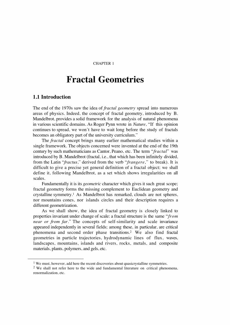
CHAPTER 1
Fractal Geometries
1.1 Introduction
The end of the 1970s saw the idea of fractal geometry spread into numerous
areas of physics. Indeed, the concept of fractal geometry, introduced by B.
Mandelbrot, provides a solid framework for the analysis of natural phenomena
in various scientific domains. As Roger Pynn wrote in Nature, “If this opinion
continues to spread, we won’t have to wait long before the study of fractals
becomes an obligatory part of the university curriculum.”
The fractal concept brings many earlier mathematical studies within a
single framework. The objects concerned were invented at the end of the 19th
century by such mathematicians as Cantor, Peano, etc. The term “fractal” was
introduced by B. Mandelbrot (fractal, i.e., that which has been infinitely divided,
from the Latin “fractus,” derived from the verb “frangere,” to break). It is
difficult to give a precise yet general definition of a fractal object; we shall
define it, following Mandelbrot, as a set which shows irregularities on all
scales.
Fundamentally it is its geometric character which gives it such great scope;
fractal geometry forms the missing complement to Euclidean geometry and
crystalline symmetry.1 As Mandelbrot has remarked, clouds are not spheres,
nor mountains cones, nor islands circles and their description requires a
different geometrization.
As we shall show, the idea of fractal geometry is closely linked to
properties invariant under change of scale: a fractal structure is the same “from
near or from far.” The concepts of self-similarity and scale invariance
appeared independently in several fields; among these, in particular, are critical
phenomena and second order phase transitions.2 We also find fractal
geometries in particle trajectories, hydrodynamic lines of flux, waves,
landscapes, mountains, islands and rivers, rocks, metals, and composite
materials, plants, polymers, and gels, etc.
1 We must, however, add here the recent discoveries about quasicrystalline symmetries.2 We shall not refer here to the wide and fundamental literature on critical phenomena,
renormalization, etc.
2 1. Fractal geometries
Many works on the subject have been published in the last 10 years. Basic
works are less numerous: besides his articles, B. Mandelbrot has published
general books about his work (Mandelbrot, 1975, 1977, and 1982); the books
by Barnsley (1988) and Falconer (1990) both approach the mathematical
aspects of the subject. Among the books treating fractals within the domain of
the physical sciences are those by Feder (1988) and Vicsek (1989) (which
particularly concentrates on growth phenomena), Takayasu (1990), or Le
Méhauté (1990), as well as a certain number of more specialized (Avnir, 1989;
Bunde and Havlin, 1991) or introductory monographs on fractals (Sapoval,
1990). More specialized reviews will be mentioned in the appropriate chapters.
1.2 The notion of dimension
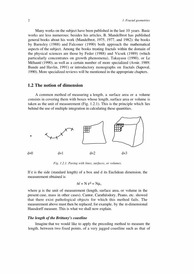
A common method of measuring a length, a surface area or a volume
consists in covering them with boxes whose length, surface area or volume is
taken as the unit of measurement (Fig. 1.2.1). This is the principle which lies
behind the use of multiple integration in calculating these quantities.
d=0 d=1 d=2 d=3
Fig. 1.2.1. Paving with lines, surfaces, or volumes.
If ! is the side (standard length) of a box and d its Euclidean dimension, the
measurement obtained is
M = N !d = Nµ,
where µ is the unit of measurement (length, surface area, or volume in the
present case, mass in other cases). Cantor, Carathéodory, Peano, etc. showed
that there exist pathological objects for which this method fails. The
measurement above must then be replaced, for example, by the "-dimensional
Hausdorff measure. This is what we shall now explain.
The length of the Brittany’s coastline
Imagine that we would like to apply the preceding method to measure the
length, between two fixed points, of a very jagged coastline such as that of
1.2 Notion of dimension 3
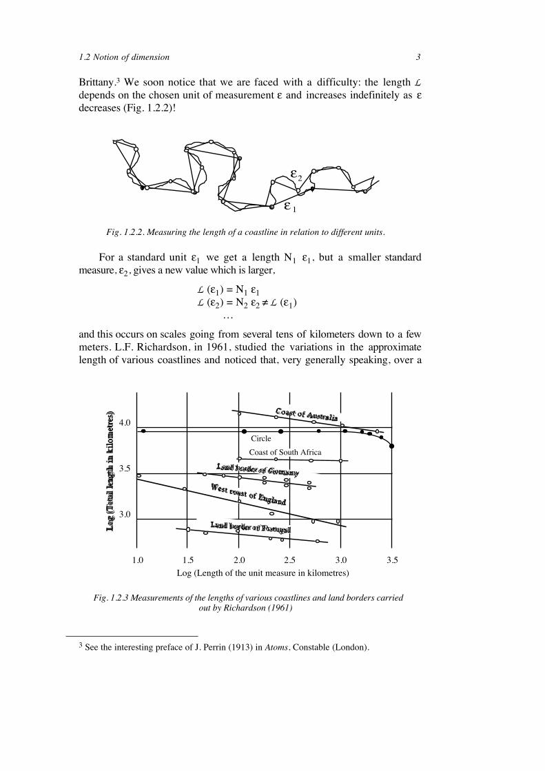
Brittany.3 We soon notice that we are faced with a difficulty: the length L
depends on the chosen unit of measurement ! and increases indefinitely as !
decreases (Fig. 1.2.2)!
!
! 1
!2
Fig. 1.2.2. Measuring the length of a coastline in relation to different units.
For a standard unit !1 we get a length N1 !1, but a smaller standard
measure, !2, gives a new value which is larger,
L (!1) = N1 !1
L (!2) = N2 !2 ! L (!1)
…
and this occurs on scales going from several tens of kilometers down to a few
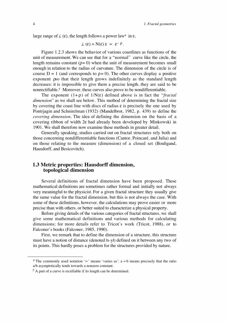
meters. L.F. Richardson, in 1961, studied the variations in the approximate
length of various coastlines and noticed that, very generally speaking, over a
!
4.0
3.5
3.0
1.0 1.5 2.0 2.5 3.0 3.5
Circle
Coast of South Africa
Log (Length of the unit measure in kilometres)
Coast of Australia
Land border of Portugal
West coast of England
Land border of Germany
Lo
g (
To
tal
len
gth
in
kil
om
etre
s)
Fig. 1.2.3 Measurements of the lengths of various coastlines and land borders carriedout by Richardson (1961)
3 See the interesting preface of J. Perrin (1913) in Atoms, Constable (London).
4 1. Fractal geometries
large range of L (!), the length follows a power law4 in !,
L (!) = N(!) ! # !– $ .
Figure 1.2.3 shows the behavior of various coastlines as functions of the
unit of measurement. We can see that for a “normal” curve like the circle, the
length remains constant ($ = 0) when the unit of measurement becomes small
enough in relation to the radius of curvature. The dimension of the circle is of
course D = 1 (and corresponds to $ = 0). The other curves display a positive
exponent $ so that their length grows indefinitely as the standard length
decreases: it is impossible to give them a precise length, they are said to be
nonrectifiable.5 Moreover, these curves also prove to be nondifferentiable.
The exponent (1+ $) of 1/N(!) defined above is in fact the “fractal
dimension” as we shall see below. This method of determining the fractal size
by covering the coast line with discs of radius ! is precisely the one used by
Pontrjagin and Schnirelman (1932) (Mandelbrot, 1982, p. 439) to define the
covering dimension. The idea of defining the dimension on the basis of a
covering ribbon of width 2! had already been developed by Minkowski in
1901. We shall therefore now examine these methods in greater detail.
Generally speaking, studies carried out on fractal structures rely both on
those concerning nondifferentiable functions (Cantor, Poincaré, and Julia) and
on those relating to the measure (dimension) of a closed set (Bouligand,
Hausdorff, and Besicovitch).
1.3 Metric properties: Hausdorff dimension, topological dimension
Several definitions of fractal dimension have been proposed. These
mathematical definitions are sometimes rather formal and initially not always
very meaningful to the physicist. For a given fractal structure they usually give
the same value for the fractal dimension, but this is not always the case. With
some of these definitions, however, the calculations may prove easier or more
precise than with others, or better suited to characterize a physical property.
Before giving details of the various categories of fractal structures, we shall
give some mathematical definitions and various methods for calculating
dimensions; for more details refer to Tricot’s work (Tricot, 1988), or to
Falconer’s books (Falconer, 1985, 1990).
First, we remark that to define the dimension of a structure, this structure
must have a notion of distance (denoted Ix-yI) defined on it between any two of
its points. This hardly poses a problem for the structures provided by nature.
4 The commonly used notation ‘#’ means ‘varies as’: a # b means precisely that the ratio
a/b asymptotically tends towards a nonzero constant.5 A part of a curve is rectifiable if its length can be determined.
1.3 Metric properties 5
We should also mention that in these definitions there is always a passage
to the limit !¯ 0. For the actual calculation of a fractal dimension we are led to
discretize (i.e., to use finite basic lengths !): the accuracy of the calculation then
depends on the relative lengths of the unit !, and that of the system (Sec. 1.4.4).
1.3.1 The topological dimension dT
If we are dealing with a geometric object composed of a set of points, we
say that its fractal dimension is dT = 0; if it is composed of line elements, dT!=
1, surface elements dT = 2, etc.
“Composed” means here that the object is locally homeomorphic to a point, a
line, a surface. The topological dimension is invariant under invertible, continuous,
but not necessarily differentiable, transformations (homeomorphisms). The
dimensions which we shall be speaking of are invariant under differentiable
transformations (dilations).
A fractal structure possesses a fractal dimension strictly greater than its
topological dimension.
1.3.2 The Hausdorff–Besicovitch dimension,
or covering dimension: dim(E)
The first approach to finding the dimension of an object, E, follows the
usual method of covering the object with boxes (belonging to the space in
which the object is embedded) whose measurement unit µ = !d(E), where d(E) is
the Euclidean dimension of the object. When d(E) is initially unknown, one
possible solution takes µ!= !" as the unit of measurement for an unknown
exponent ". Let us consider, for example, a square (d = 2) of side L, and cover
it with boxes of side !. The measure is given by M = Nµ, where N is the
number of boxes, hence N = (L/!)d. Thus,
M = N !" = (L/!)d !" = L2 !"#2
If we try " = 1, we find that M $ % when ! $ 0: the “length” of a square
is infinite. If we try " = 3, we find that M $ 0 when ! $ 0: the “volume” of a
square is zero. The surface area of a square is obtained only when " = 2, and
its dimension is the same as that of a surface d = " = 2.
The fact that this method can be applied for any real " is very interesting
as it makes possible its generalization to noninteger dimensions.
We can formalize this measure a little more. First, as the object has no
specific shape, it is not possible, in general, to cover it with identical boxes of
side !. But the object E may be covered with balls Vi whose diameter (diam Vi)
is less than or equal to !. This offers more flexibility, but requires that the
inferior limit of the sum of the elementary measures be taken as µ =
(diam!Vi)".
6 1. Fractal geometries
Therefore, we consider what is called the "–covering measure (Hausdorff,
1919; Besicovitch, 1935) defined as follows:
m"(E) = lim !$0 inf{ "(diam Vi)" : &Vi 'E, diam Vi # !}, (1.3-1)
and we define the Hausdorff (or Hausdorff–Besicovitch) dimension: dim E by
dim E = inf { " : m"(E) = 0 }
= sup { " : m"(E) = $}. (1.3-2)
The Hausdorff dimension is the value of " for which the measure jumps from
zero to infinity. For the value " = dim E, this measure may be anywhere
between zero and infinity.
The function m"(E) is monotone in the sense that if a set F is included in E,
E ' F, then m"(E) % m"(F) whatever the value of ".
1.3.3 The Bouligand–Minkowski dimension
We can also define a dimension known as the Bouligand–Minkowski
dimension (Bouligand, 1929; Minkowski, 1901), denoted &(E). Here are some
methods of calculating &(E):
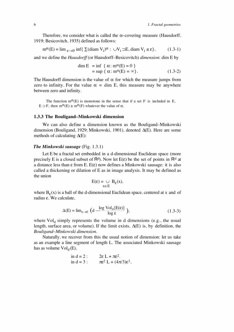
The Minkowski sausage (Fig. 1.3.1)
Let E be a fractal set embedded in a d-dimensional Euclidean space (more
precisely E is a closed subset of Rd). Now let E(!) be the set of points in Rd at
a distance less than ! from E. E(!) now defines a Minkowski sausage: it is also
called a thickening or dilation of E as in image analysis. It may be defined as
the union
E(!) = & B!(x),
x(E
where B!(x) is a ball of the d-dimensional Euclidean space, centered at x and of
radius !. We calculate,
!(E) = lim"#0 (d –log Vold [E(")]
log " ), (1.3-3)
where Vold simply represents the volume in d dimensions (e.g., the usual
length, surface area, or volume). If the limit exists, &(E) is, by definition, the
Bouligand–Minkowski dimension.
Naturally, we recover from this the usual notion of dimension: let us take
as an example a line segment of length L. The associated Minkowski sausage
has as volume Vold (E),
in d = 2 : 2! L + '!2,
in d = 3 : '!2 L + (4'/3)!3,
!
1.3 Metric properties 7
Fig. 1.3.1. Minkowski sausage or thickening of a curve E.
so that neglecting higher orders in !, Vold (E) ) ! d – 1.
In general terms we have:
If E is a point: Vold (E) ) !d, *(E) = 0.
If E is a rectifiable arc: Vold (E) ) !d – 1, *(E) = 1.
If E is a k-dimensional ball: Vold (E) ) !d – k, *(E) = k.
In practice, &(E) is obtained as the slope of the line of least squares of the
set of points given by the plane coordinates,
{ log 1/!, log Vold [E(!) /!d ] }.
This method is easy to use. The edge effects (like those obtained above in
measuring a segment of length L) lead to a certain inaccuracy in practice (i.e., to
a curve for values of ! which are not very small).
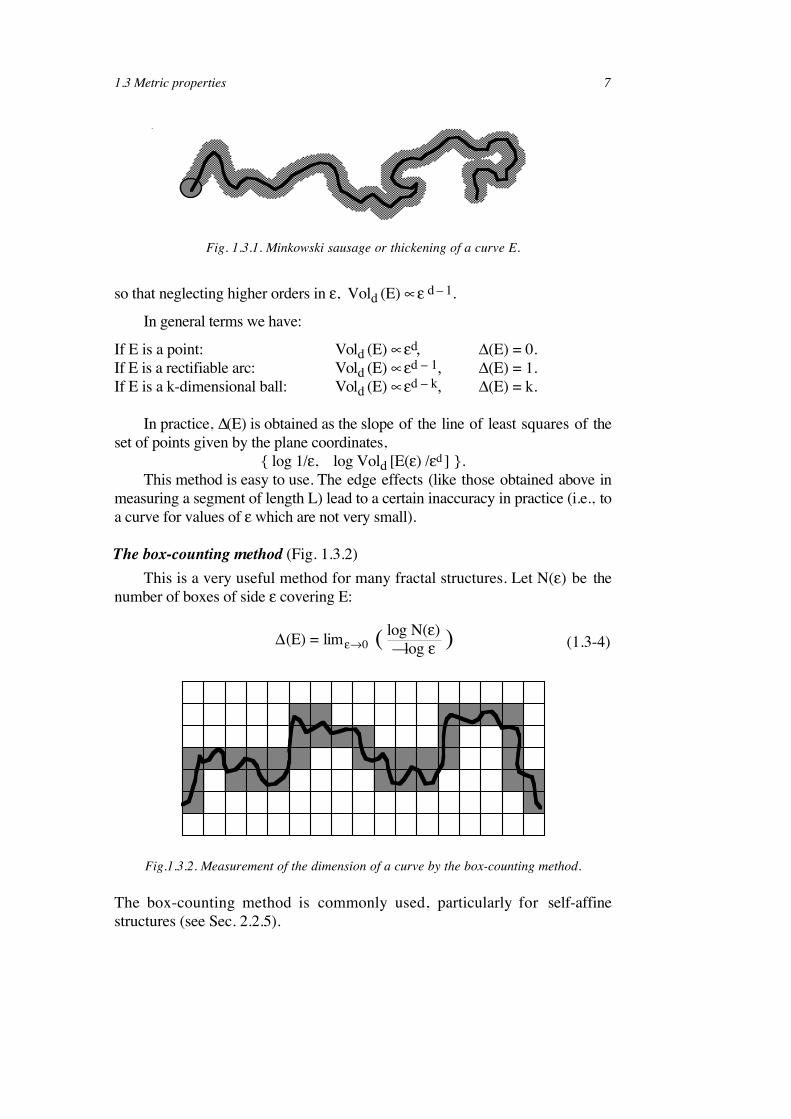
The box-counting method (Fig. 1.3.2)
This is a very useful method for many fractal structures. Let N(!) be the
number of boxes of side ! covering E:
!(E) = lim"#0 (log N(")
– log ")
(1.3-4)
!
Fig.1.3.2. Measurement of the dimension of a curve by the box-counting method.
The box-counting method is commonly used, particularly for self-affine
structures (see Sec. 2.2.5).
8 1. Fractal geometries
The dimension of a union of sets is equal to the largest of the dimensions of these
sets: &(E&F) = max {&(E), &(F)}.
The limit &(E) may depend on the choice of paving. If there are two different
limits Sup and Inf, the Sup limit should be taken.
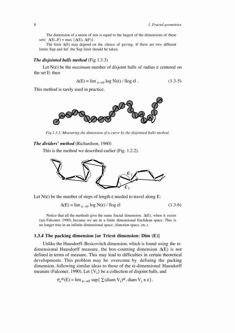
The disjointed balls method (Fig 1.3.3)
Let N(!) be the maximum number of disjoint balls of radius ! centered on
the set E: then
*(E) = lim !$0 log N(!) / |log !| . (1.3-5)
This method is rarely used in practice.!
Fig.1.3.3. Measuring the dimension of a curve by the disjointed balls method.
The dividers’ method (Richardson, 1960)
This is the method we described earlier (Fig. 1.2.2).!
!1
!2
Let N(!) be the number of steps of length ! needed to travel along E:
*(E) = lim !$0 log N(!) / |log !| (1.3-6)
Notice that all the methods give the same fractal dimension, &(E), when it exists
(see Falconer, 1990), because we are in a finite dimensional Euclidean space. This is
no longer true in an infinite dimensional space, (function space, etc.).
1.3.4 The packing dimension [or Tricot dimension: Dim (E)]
Unlike the Hausdorff–Besicovitch dimension, which is found using the "-
dimensional Hausdorff measure, the box-counting dimension &(E) is not
defined in terms of measure. This may lead to difficulties in certain theoretical
developments. This problem may be overcome by defining the packing
dimension, following similar ideas to those of the "-dimensional Hausdorff
measure (Falconer, 1990). Let {Vi} be a collection of disjoint balls, and
Po"(E) = lim !$0 sup{ "(diam Vi)
", diam Vi # !}.
1.3 Metric properties 9
As this expression is not always a measure we must consider
P!(E) = inf{ P
o
!
(E i ) :!"i =1
Ei#E} .
The packing dimension is defined by the following limit:
Dim E = sup{" : P "(E) = $ } = inf {" : P
"(E) = 0 }, (1.3-7a)
alternatively, according to the previous definitions:
Dim E = inf{sup *(Ei) : & Ei ' E}. (1.3-7b)
The following inequalities between the various dimensions defined above are
always true:
dim E # Dim E # * (E)
dim E + dim F # dim E+F
# dim E + Dim F
# Dim E+F # Dim E + Dim F.
Notice that for multifractals box-counting dimensions are in practice rather Tricot
dimensions.
Other methods of calculation have been proposed by Tricot (Tricot, 1982)
which could prove attractive in certain situations. Without entering into the
details, we should also mention the method of structural elements, the method
of variations and the method of intersections.
Theorem: If there exists a real D and a finite positive measure µ such that for
all x(E, (Br(x) being the ball of radius r centered at x),
log µ[Br(x)]/log r $ D, then
D = dim E. (1.3-8)
D is also called the mass dimension. If the convergence is uniform on E, then
D = dim(E) = *(E). (1.3-9)
This theorem does not always apply: dim E = 0 for a denumerable set, while for
the Bouligand–Minkowski dimension *(E) ( 0.
In practice, Mandelbrot has popularized the Hausdorff–Besicovitch
dimension or mass dimension (as the measure is very often a mass), dim E,
which turns out to be one of the simpler and more understandable dimensions
(although not always the most appropriate) for the majority of problems in
physics when the above theorem applies.
So we now have the following relation giving the mass inside a ball of
radius r,
10 1. Fractal geometries
M = µ(Br (x)) ! r D , (1.3-10)
where the center x of the ball B is inside the fractal structure E.
We shall of course take the physicist’s point of view and not burden
ourselves, at first, with too much mathematical rigor. The fractal dimension will
in general be denoted D and, in the cases considered, we shall suppose that,
unless specified otherwise, the existence theorem applies and therefore that the
fractal dimension is the same for all the methods described above.
Units of measure
The above relation can often be written in the form of a dimensionless
equation, by introducing the unit of length !u and volume (!u)d or mass ,u =
(!u)d , (by assuming a uniform density , over the support):
V
(!u ) d
or M"u
# r!u
D .
Examples of this for the Koch curve and the Sierpinski gasket will be
given later in Sec. 1.4.1. In this case the unit of volume is that of a space with
dimension equal to the topological dimension of the geometric objects making
up the set (see Sec. 1.3.1).
From a strictly mathematical point of view the term “dimension” should be
reserved for sets. For measures, we can think of the set covered by a uniform measure.
However, we can define the dimension of a measure by
dim(µ) = inf { dim(A), µ(Ac)=0 },
A being a measurable set and Ac its complement. This dimension is often strictly less
than the dimension of the support. This happens with the information dimension
described in Sec. 1.6.2.
For objects with a different scaling factor in different spatial directions, the box-
counting dimension differs from the Hausdorff dimension (see Fig. 2.2.8).
Having defined the necessary tools for studying fractal structures, it is now
time to get to the heart of the matter by giving the first concrete examples of
fractals.
1.4 Examples of fractals
1.4.1 Deterministic fractals
Some fractal structures are constructed simply by using an iterative
process consisting of an initiator (initial state) and a generator (iterative
operation).
1.4 Examples of fractals 11
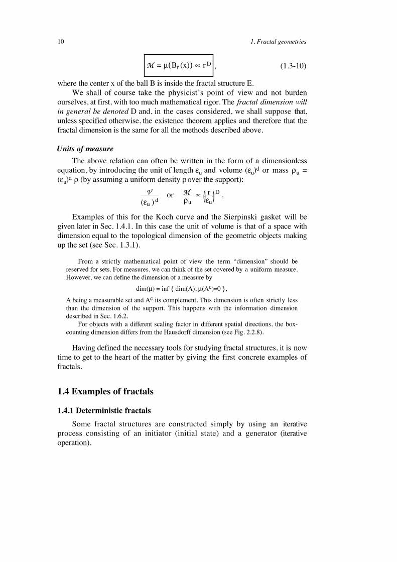
The triadic Von Koch curve (1904)Each segment of length ε is replaced by a broken line (generator),
composed of four segments of length ε/3, according to the following recurrencerelation:
(generator)
At iteration zero, we have an initiator which is a segment in the case of thetriadic Koch curve, or an equilateral triangle in the case of the Koch island. Ifthe initiator is a segment of horizontal length L, at the first iteration (the curvecoincides with the generator) the base segments will have length ε1 = L/3;
at the second iteration they will have length ε2 = L/9 as each segment is againreplaced by the generator, then ε3 = L/33 at the third iteration
,
and so on. The relations giving the length L of the curve are thus
ε1 = L/3 → L1 = 4 ε1ε2 = L/9 → L2 = 16 ε2
…εn = L/3n → Ln = 4n εn
by eliminating n from the two equations in the last line, the length Ln may bewritten as a function of the measurement unit εn
Ln= LD (εn )1–D where D = log 4 / log 3 = 1.2618…
For a fixed unit length εn, Ln grows as the Dth power of the size L of the curve.Notice that here again we meet the exponent ρ = D–1 of εn, which we first metin Sec. 1.2 (Richardson's law) and which shows the divergence of Ln as εn →0.
12 1. Fractal geometries
At a given iteration, the curve obtained is not strictly a fractal but according toMandelbrot’s term a “prefractal”. A fractal is a mathematical object obtained in thelimit of a series of prefractals as the number of iterations n tends to infinity. Ineveryday language, prefractals are often both loosely called “fractals”.
The previous expression is the first example given of a scaling law whichmay be written
Ln / εn = f (L /εn ) = ( L /εn )D . (1.4-1)
A scaling law is a relation between different dimensionless quantitiesdescribing the system, (the relation here is a simple power law). Such a law isgenerally possible only when there is a single independent unit of length in theobject (here εn).
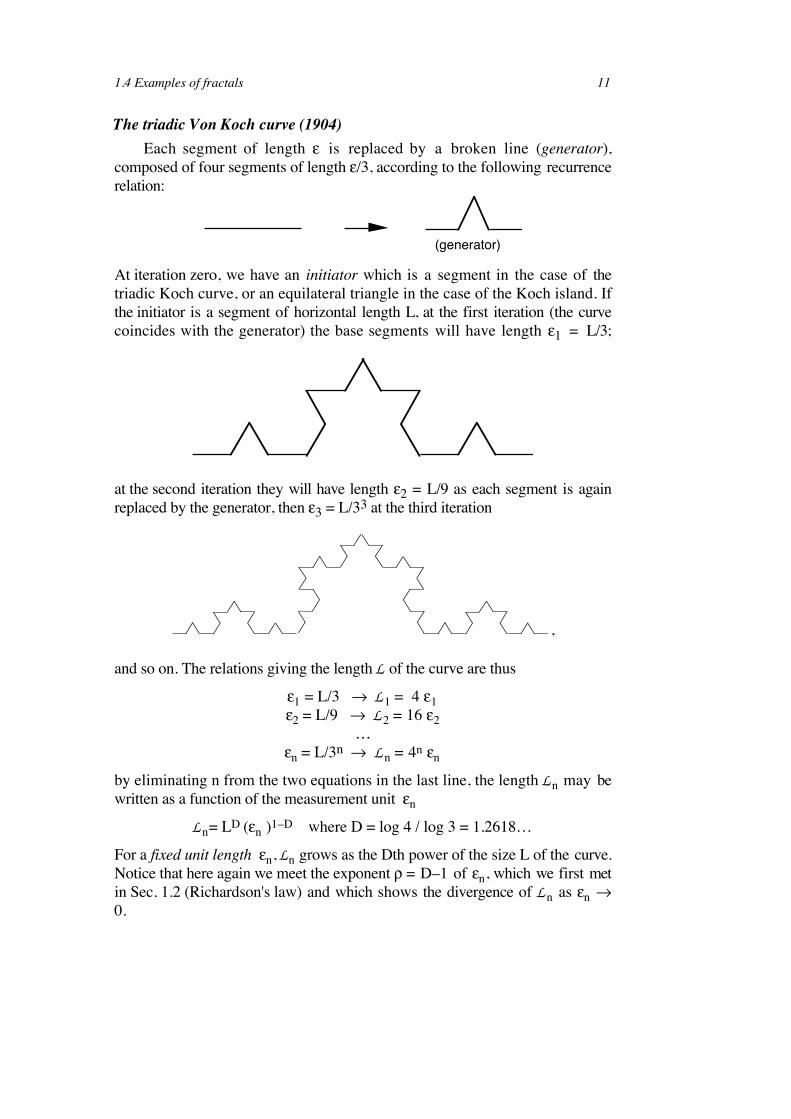
A structure associated with the Koch curve is obtained by choosing anequilateral triangle as initiator. The structure generated in this way is the well-known Koch island (see Fig. 1.4.1).
Fig. 1.4.1. Koch island after only three iterations. Its coastline is fractal, but the island itself has dimension 2 (it is said to be a surface fractal).
Simply by varying the generator, the Koch curve may be generalized togive curves with fractal dimension 1 ≤ D ≤ 2. A straightforward example isprovided by the modified Koch curve whose generator is
α
and whose fractal dimension is D = log 4 / log [2 + 2 sin(α/2)]. Notice that inthe limit α = 0 we have D = 2, that is to say a curve which fills a triangle. It isnot exactly a curve as it has an infinite number of multiple points. But theconstruction can be slightly modified to eliminate them. The dimension D = 2
1.4 Examples of fractals 13
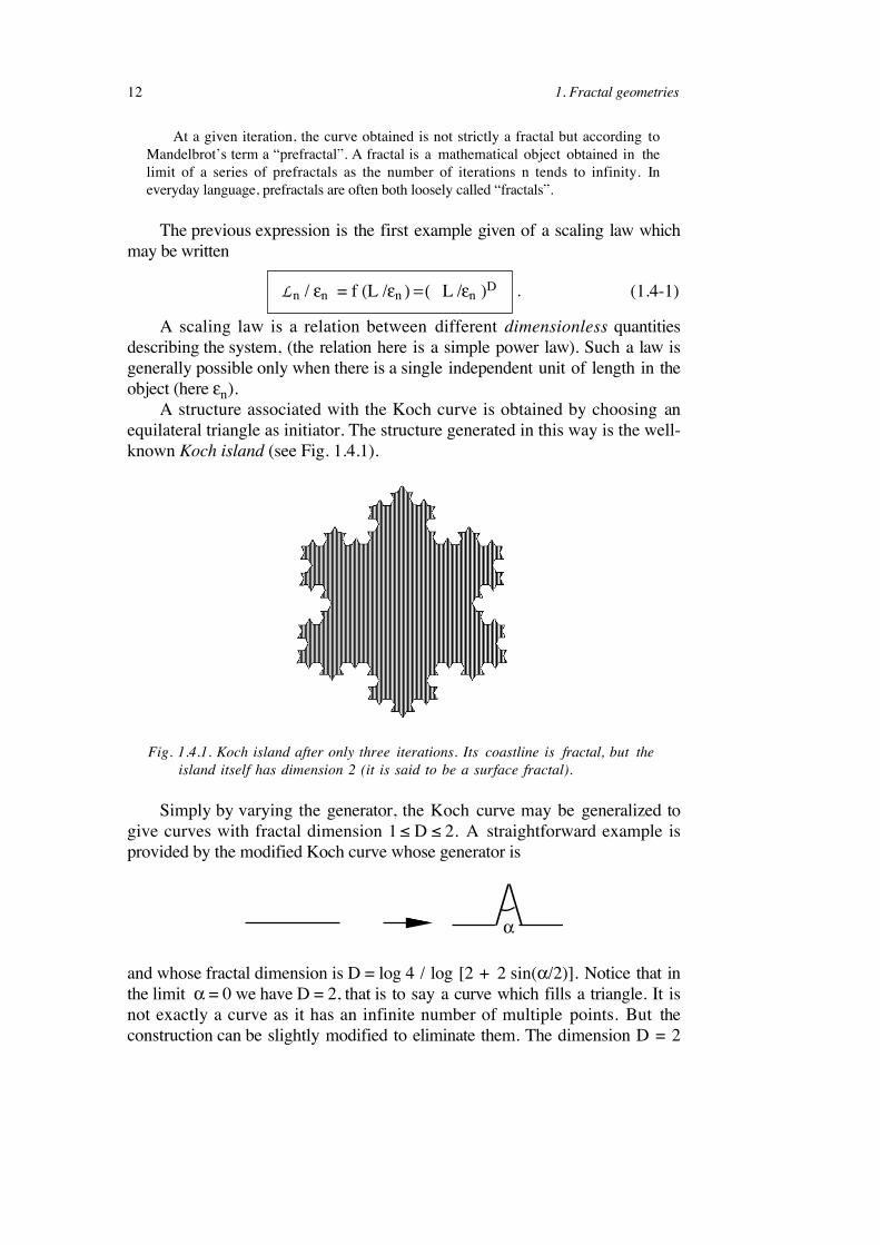
(= log 9/log 3) is also obtained for the Peano curve (Fig. 1.4.2) (which isdense in a square) whose generator is formed from 9 segments with a changeby a factor 3 in the linear dimension, i.e.,
.
This gives after the first three iterations,
Fig. 1.4.2. First three iterations of the Peano curve (for graphical reasons the scale issimultaneously dilated at each iteration by a factor of 3). The Peano curve is dense in
the plane and its fractal dimension is 2.
This construction has also been modified (rounding the angles) to eliminatedouble points.
The von Koch and Peano curves are as their name indicates: curves, that is,their topological dimension is
dT = 1.
Practical determination of the fractal dimensionusing the mass-radius relation
As mentioned earlier, a method which we shall be using frequently todetermine fractal dimensions6 consists in calculating the mass of the structurewithin a ball of dimension d centered on the fractal. If the embedding space isd-dimensional, and of radius R, then
M ∝ RD .
The measure here is generally a mass, but it could equally well be a “surfacearea” or any other scalar quantity attached to the support (Fig. 1.4.3).
6 The box-counting method will also be frequently used.
14 1. Fractal geometries
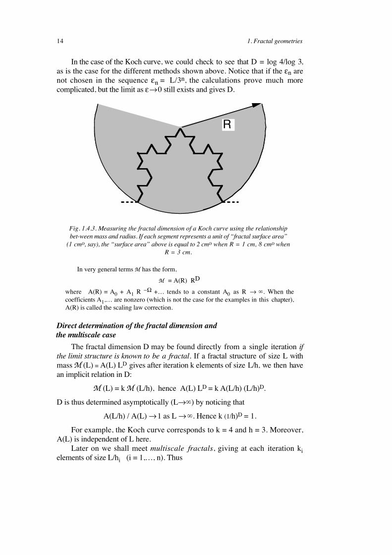
In the case of the Koch curve, we could check to see that D = log 4/log 3,as is the case for the different methods shown above. Notice that if the εn arenot chosen in the sequence εn = L/3n, the calculations prove much morecomplicated, but the limit as ε → 0 still exists and gives D.
R
Fig. 1.4.3. Measuring the fractal dimension of a Koch curve using the relationshipbet-ween mass and radius. If each segment represents a unit of “fractal surface area”
(1 cmD, say), the “surface area” above is equal to 2 cmD when R = 1 cm, 8 cmD whenR = 3 cm.
In very general terms M has the form,M = A(R) RD
where A(R) = A0 + A1 R −Ω +… tends to a constant A0 as R → ∞. When thecoefficients A1,… are nonzero (which is not the case for the examples in this chapter),A(R) is called the scaling law correction.
Direct determination of the fractal dimension andthe multiscale case
The fractal dimension D may be found directly from a single iteration ifthe limit structure is known to be a fractal. If a fractal structure of size L withmass M (L) = A(L) LD gives after iteration k elements of size L/h, we then havean implicit relation in D:
M (L) = k M (L/h), hence A(L) LD = k A(L/h) (L/h)D.
D is thus determined asymptotically (L→∞) by noticing that
A(L/h) / A(L) → 1 as L → ∞. Hence k (1/h)D = 1.
For example, the Koch curve corresponds to k = 4 and h = 3. Moreover,A(L) is independent of L here.
Later on we shall meet multiscale fractals, giving at each iteration kielements of size L/hi (i = 1,…, n). Thus
1.4 Examples of fractals 15
M (L) =k1 M (L/h1) + k2 M (L/h2) +...+ kn M (L/hn),
which means that the mass of the object of linear size L is the sum of ki massesof similar objects of size L/hi. Thus,
k1 (1/h1)D + k2 (1/h2)D… + kn (1/hn)D = 1, (1.4-2)
which determines D.
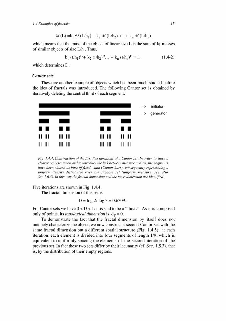
Cantor setsThese are another example of objects which had been much studied before
the idea of fractals was introduced. The following Cantor set is obtained byiteratively deleting the central third of each segment:
⇒⇒
initiatorgenerator
Fig. 1.4.4. Construction of the first five iterations of a Cantor set. In order to have aclearer representation and to introduce the link between measure and set, the segmentshave been chosen as bars of fixed width (Cantor bars), consequently representing auniform density distributed over the support set (uniform measure, see alsoSec.1.6.3). In this way the fractal dimension and the mass dimension are identified.
Five iterations are shown in Fig. 1.4.4.The fractal dimension of this set is
D = log 2/ log 3 = 0.6309...
For Cantor sets we have 0 < D < 1: it is said to be a “dust.” As it is composedonly of points, its topological dimension is dT = 0.
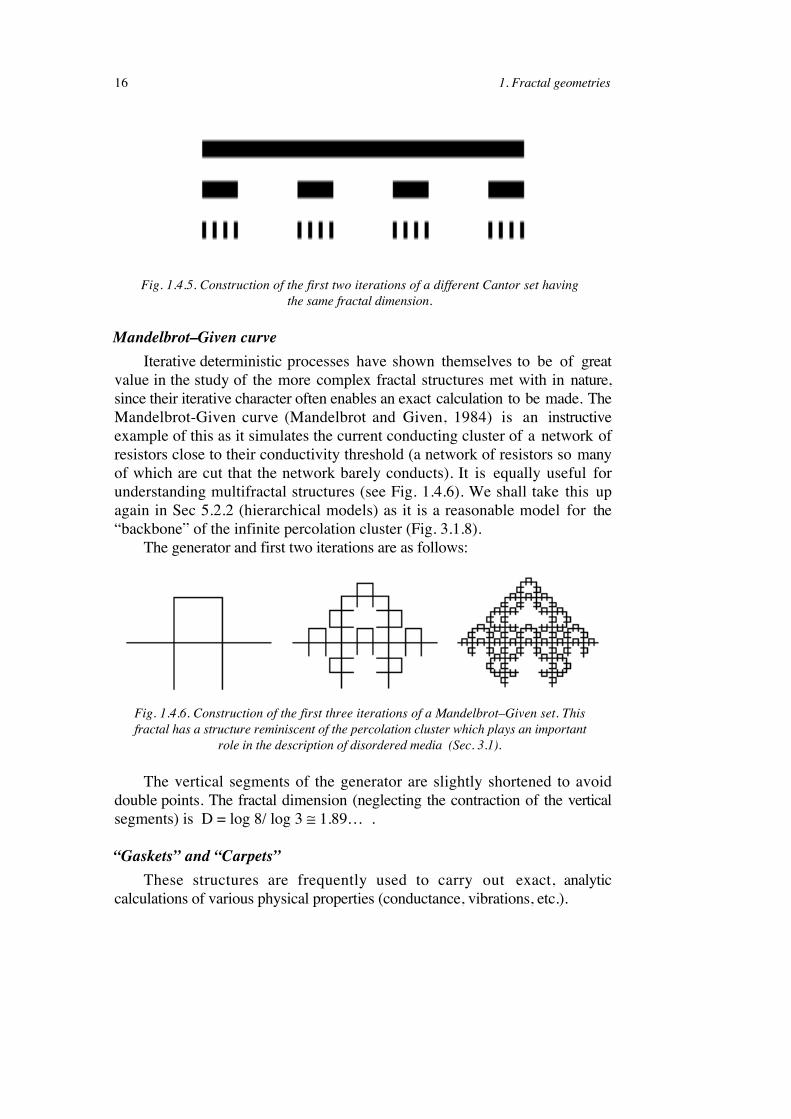
To demonstrate the fact that the fractal dimension by itself does notuniquely characterize the object, we now construct a second Cantor set with thesame fractal dimension but a different spatial structure (Fig. 1.4.5): at eachiteration, each element is divided into four segments of length 1/9, which isequivalent to uniformly spacing the elements of the second iteration of theprevious set. In fact these two sets differ by their lacunarity (cf. Sec. 1.5.3), thatis, by the distribution of their empty regions.
16 1. Fractal geometries
Fig. 1.4.5. Construction of the first two iterations of a different Cantor set havingthe same fractal dimension.
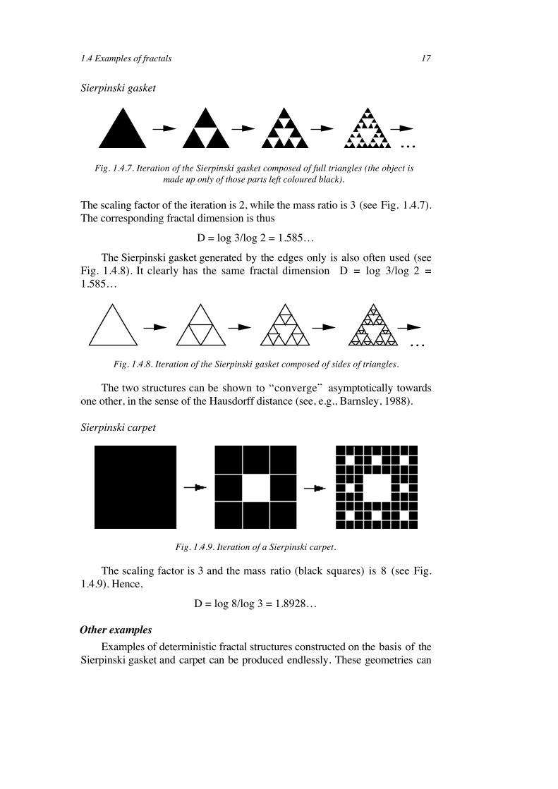
Mandelbrot–Given curveIterative deterministic processes have shown themselves to be of great
value in the study of the more complex fractal structures met with in nature,since their iterative character often enables an exact calculation to be made. TheMandelbrot-Given curve (Mandelbrot and Given, 1984) is an instructiveexample of this as it simulates the current conducting cluster of a network ofresistors close to their conductivity threshold (a network of resistors so manyof which are cut that the network barely conducts). It is equally useful forunderstanding multifractal structures (see Fig. 1.4.6). We shall take this upagain in Sec 5.2.2 (hierarchical models) as it is a reasonable model for the“backbone” of the infinite percolation cluster (Fig. 3.1.8).
The generator and first two iterations are as follows:
Fig. 1.4.6. Construction of the first three iterations of a Mandelbrot–Given set. Thisfractal has a structure reminiscent of the percolation cluster which plays an important
role in the description of disordered media (Sec. 3.1).
The vertical segments of the generator are slightly shortened to avoiddouble points. The fractal dimension (neglecting the contraction of the verticalsegments) is D = log 8/ log 3 ≅ 1.89… .
“Gaskets” and “Carpets”These structures are frequently used to carry out exact, analytic
calculations of various physical properties (conductance, vibrations, etc.).
1.4 Examples of fractals 17
Sierpinski gasket
Fig. 1.4.7. Iteration of the Sierpinski gasket composed of full triangles (the object ismade up only of those parts left coloured black).
The scaling factor of the iteration is 2, while the mass ratio is 3 (see Fig. 1.4.7).The corresponding fractal dimension is thus
D = log 3/log 2 = 1.585…
The Sierpinski gasket generated by the edges only is also often used (seeFig. 1.4.8). It clearly has the same fractal dimension D = log 3/log 2 =1.585…
Fig. 1.4.8. Iteration of the Sierpinski gasket composed of sides of triangles.
The two structures can be shown to “converge” asymptotically towardsone other, in the sense of the Hausdorff distance (see, e.g., Barnsley, 1988).
Sierpinski carpet
Fig. 1.4.9. Iteration of a Sierpinski carpet.
The scaling factor is 3 and the mass ratio (black squares) is 8 (see Fig.1.4.9). Hence,
D = log 8/log 3 = 1.8928…
Other examplesExamples of deterministic fractal structures constructed on the basis of the
Sierpinski gasket and carpet can be produced endlessly. These geometries can
18 1. Fractal geometries
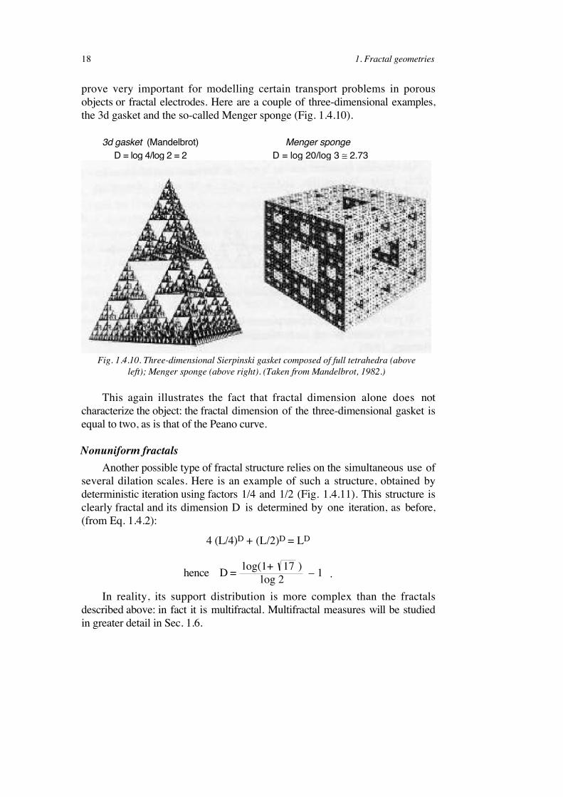
prove very important for modelling certain transport problems in porousobjects or fractal electrodes. Here are a couple of three-dimensional examples,the 3d gasket and the so-called Menger sponge (Fig. 1.4.10).
3d gasket (Mandelbrot) Menger sponge D = log 4/log 2 = 2 D = log 20/log 3 ≅ 2.73
Fig. 1.4.10. Three-dimensional Sierpinski gasket composed of full tetrahedra (aboveleft); Menger sponge (above right). (Taken from Mandelbrot, 1982.)
This again illustrates the fact that fractal dimension alone does notcharacterize the object: the fractal dimension of the three-dimensional gasket isequal to two, as is that of the Peano curve.
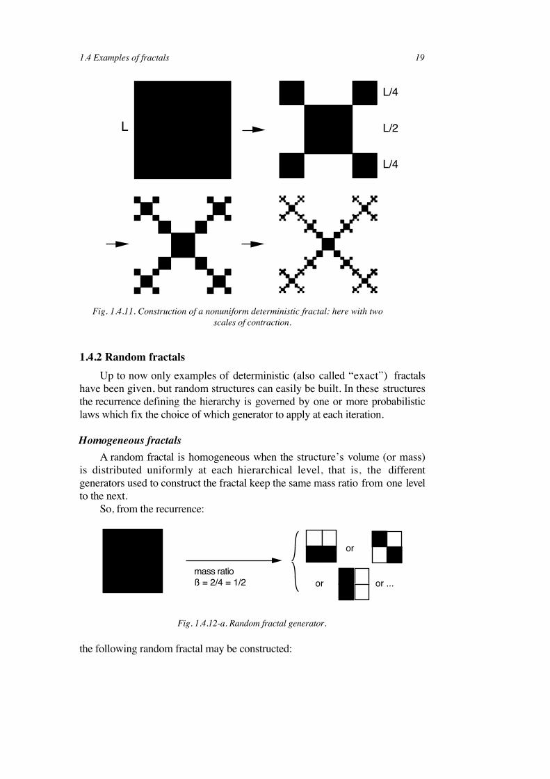
Nonuniform fractalsAnother possible type of fractal structure relies on the simultaneous use of
several dilation scales. Here is an example of such a structure, obtained bydeterministic iteration using factors 1/4 and 1/2 (Fig. 1.4.11). This structure isclearly fractal and its dimension D is determined by one iteration, as before,(from Eq. 1.4.2):
4 (L/4)D + (L/2)D = LD
D = log(1+ 17 )log 2 – 1hence
.
In reality, its support distribution is more complex than the fractalsdescribed above: in fact it is multifractal. Multifractal measures will be studiedin greater detail in Sec. 1.6.
1.4 Examples of fractals 19
L
L/4
L/2
L/4
Fig. 1.4.11. Construction of a nonuniform deterministic fractal: here with twoscales of contraction.
1.4.2 Random fractalsUp to now only examples of deterministic (also called “exact”) fractals
have been given, but random structures can easily be built. In these structuresthe recurrence defining the hierarchy is governed by one or more probabilisticlaws which fix the choice of which generator to apply at each iteration.
Homogeneous fractalsA random fractal is homogeneous when the structure’s volume (or mass)
is distributed uniformly at each hierarchical level, that is, the differentgenerators used to construct the fractal keep the same mass ratio from one levelto the next.
So, from the recurrence:
mass ratio ß = 2/4 = 1/2 or ...
or
or
Fig. 1.4.12-a. Random fractal generator.
the following random fractal may be constructed:
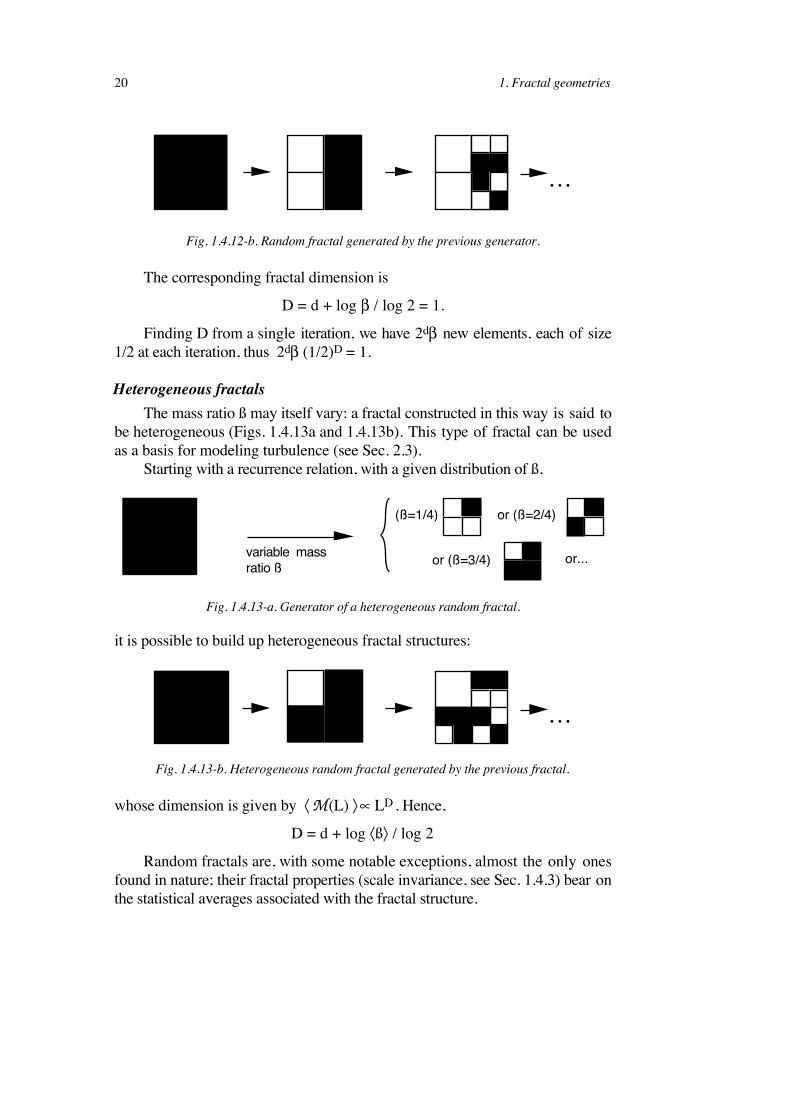
20 1. Fractal geometries
…
Fig. 1.4.12-b. Random fractal generated by the previous generator.
The corresponding fractal dimension is
D = d + log β / log 2 = 1.
Finding D from a single iteration, we have 2dβ new elements, each of size1/2 at each iteration, thus 2dβ (1/2)D = 1.
Heterogeneous fractalsThe mass ratio ß may itself vary: a fractal constructed in this way is said to
be heterogeneous (Figs. 1.4.13a and 1.4.13b). This type of fractal can be usedas a basis for modeling turbulence (see Sec. 2.3).
Starting with a recurrence relation, with a given distribution of ß,
variable mass ratio ß or...or (ß=3/4)
(ß=1/4) or (ß=2/4)
Fig. 1.4.13-a. Generator of a heterogeneous random fractal.
it is possible to build up heterogeneous fractal structures:
…
Fig. 1.4.13-b. Heterogeneous random fractal generated by the previous fractal.
whose dimension is given by 〈 M(L) 〉 ∝ LD . Hence,
D = d + log 〈ß〉 / log 2
Random fractals are, with some notable exceptions, almost the only onesfound in nature; their fractal properties (scale invariance, see Sec. 1.4.3) bear onthe statistical averages associated with the fractal structure.
1.4 Examples of fractals 21
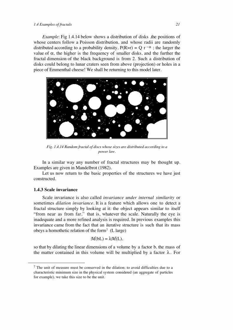
Example: Fig 1.4.14 below shows a distribution of disks ,the positions ofwhose centers follow a Poisson distribution, and whose radii are randomlydistributed according to a probability density, P(R>r) = Q r − α ; the larger thevalue of α, the higher is the frequency of smaller disks, and the further thefractal dimension of the black background is from 2. Such a distribution ofdisks could belong to lunar craters seen from above (projection) or holes in apiece of Emmenthal cheese! We shall be returning to this model later.
Fig. 1.4.14 Random fractal of discs whose sizes are distributed according to apower law.
In a similar way any number of fractal structures may be thought up.Examples are given in Mandelbrot (1982).
Let us now return to the basic properties of the structures we have justconstructed.
1.4.3 Scale invarianceScale invariance is also called invariance under internal similarity or
sometimes dilation invariance. It is a feature which allows one to detect afractal structure simply by looking at it: the object appears similar to itself“from near as from far,” that is, whatever the scale. Naturally the eye isinadequate and a more refined analysis is required. In previous examples thisinvariance came from the fact that an iterative structure is such that its massobeys a homothetic relation of the form7 (L large)
M(bL) = λM(L),
so that by dilating the linear dimensions of a volume by a factor b, the mass ofthe matter contained in this volume will be multiplied by a factor λ . For
7 The unit of measure must be conserved in the dilation; to avoid difficulties due to acharacteristic minimum size in the physical system considered (an aggregate of particlesfor example), we take this size to be the unit.
22 1. Fractal geometries
ordinary surfaces or volumes λ = bd, where d is the dimension of the object.This relation generalizes to all self-similar fractals. For the Koch curve, forexample,
M(3L) = 4M(L) = 3DM(L),
and in the general case, M ( bL) = bD M ( L) . (1.4-3)
This is a very direct method of calculating D, which is thus also the similaritydimension, (see also the remark p. 14).
The scale invariance relation M(bL) = bD M(L) is equivalent to the mass/radiusrelation M(L) = A0LD. To see this, choose b = 1/L in the scaling law, giving M(L) =M(1) LD.
We shall see that internal similarity is present in many exact or randomfractals (see below), which are not generated by iteration.
Generally speaking:Translational invariance → periodic networksDilation invariance → self-similar fractals
In practice scale invariance only works for a limited range of distances r:
a << r << Λ.
Λ is the macroscopic limit due to the size of the sample, correlation length,effects of gradients, etc. and a is the microscopic limit due to the lattice distance,molecular sizes, etc. When we come to discuss macroscopic structures inchapter 2 (and microscopic structures in chapter 3), we mean to say that thescales of a and Λ are macroscopic (or microscopic, respectively). Moreover, ifthere are corrections to the scaling law [A(r) not constant], scale invariance willonly be found asymptotically (for very large r).
1.4.4 Ambiguities in practical measurementsIn practice, in other words, for physical objects, we find problems in
applying the methods we have just described. This is partly because, as wementioned in the last paragraph, there is both a minimum characteristic sizebelow which the fractal description ceases to be valid (for example, aggregatescomposed of small particles) and also an upper size limit for the object underconsideration. But it is also because a physical phenomenon, dependent onsome (dominant) parameter, only generates fractal structures on all scales for acritical value of this parameter. This value is often difficult to attain, so scalinglaw corrections are generally required (see remark p. 14).
1.5 Connectivity properties 23
The fractal dimension is obtained from the slope of the linear regression of
the points with coordinates, {log 1/r, log N(r)}, with r going from the minimum
characteristic size to the size of the object.
The method employed to determine the dimension (discussed by Tricot,
1982), the limited extent of a fractal dynamic (object only fractal over a scale
spanning less than two orders of magnitude), and the presence of scaling law
corrections, all contribute to making this method based on log-log regression
sometimes imprecise. Such a representation tends to straighten any curves. The
presence of slight curvature is a sign that the asymptotic régime has not been
reached. Furthermore, as a point of inflexion may be taken for linear behavior,
it is not always obvious, without reliable theoretical support, what is happening
in this case. A good theoretical model or a dynamic that extends over a
sufficiently wide range of scales is therefore indispensable. A discussion about
real and apparent power laws may be found in T. A. Witten, Les Houches,
1985 (Boccara and Daoud, 1985).
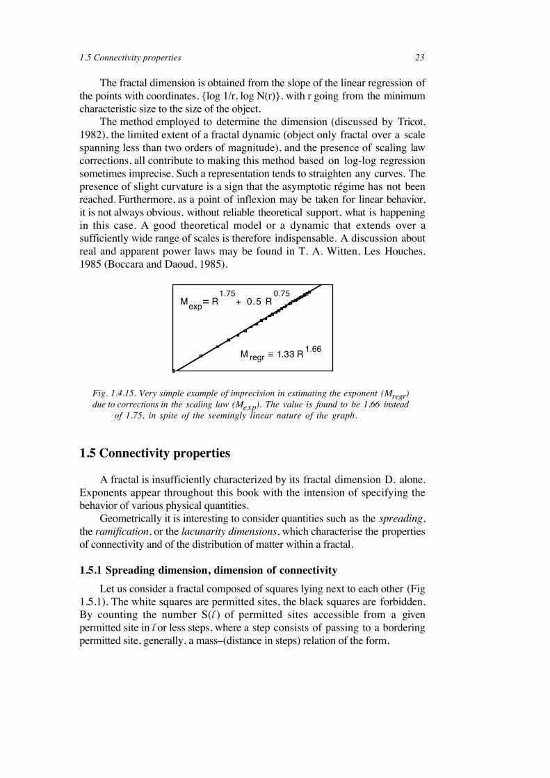
Mexp= R + 0.5 R
M ! .33 Rregr1.66!
0.75!1.75!
1
Fig. 1.4.15. Very simple example of imprecision in estimating the exponent (Mregr)
due to corrections in the scaling law (Mexp). The value is found to be 1.66 instead
!!!!!!!!!of 1.75, in spite of the seemingly linear nature of the graph.
1.5 Connectivity properties
A fractal is insufficiently characterized by its fractal dimension D, alone.
Exponents appear throughout this book with the intension of specifying the
behavior of various physical quantities.
Geometrically it is interesting to consider quantities such as the spreading,
the ramification, or the lacunarity dimensions, which characterise the properties
of connectivity and of the distribution of matter within a fractal.
1.5.1 Spreading dimension, dimension of connectivity
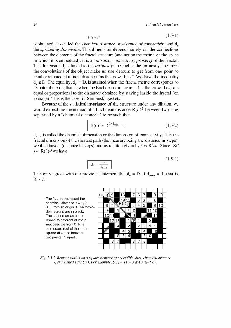
Let us consider a fractal composed of squares lying next to each other (Fig
1.5.1). The white squares are permitted sites, the black squares are forbidden.
By counting the number S(l ) of permitted sites accessible from a given
permitted site in l or less steps, where a step consists of passing to a bordering
permitted site, generally, a mass–(distance in steps) relation of the form,
24 1. Fractal geometries
S(l ) ! l de(1.5-1)
is obtained. l is called the chemical distance or distance of connectivity and de
the spreading dimension. This dimension depends solely on the connections
between the elements of the fractal structure (and not on the metric of the space
in which it is embedded): it is an intrinsic connectivity property of the fractal.
The dimension ds is linked to the tortuosity: the higher the tortuosity, the more
the convolutions of the object make us use detours to get from one point to
another situated at a fixed distance “as the crow flies.” We have the inequality
de ! D. The equality, de = D, is attained when the fractal metric corresponds to
its natural metric, that is, when the Euclidean dimensions (as the crow flies) are
equal or proportional to the distances obtained by staying inside the fractal (on
average). This is the case for Sierpinski gaskets.
Because of the statistical invariance of the structure under any dilation, we
would expect the mean quadratic Euclidean distance R(l )2 between two sites
separated by a “chemical distance” l to be such that
R(l )2 ! l 2/dmin . (1.5-2)
dmin is called the chemical dimension or the dimension of connectivity. It is the
fractal dimension of the shortest path (the measure being the distance in steps):
we then have a (distance in steps)–radius relation given by l ! Rdmin. Since S(l
) ! R(l )D we have
de = D
dmin
(1.5-3)
This only agrees with our previous statement that de = D, if dmin = 1, that is,
R"! l.
spond to different clusters
inaccessible from 0. R is
The figures represent the
chemical distance = 1, 2,
3,... from an origin 0.The forbid-
den regions are in black.
The shaded areas corre-
the square root of the mean
square distance between
two points, apart .!l
!l
11 5
2345 119
1110
6910 13 77 9 10
148 5 6 7 815
3 4 5 9 1078 6
14
13
78 678
2 2 3
43
4
34
4
56 5 6
5
6
12 1 1 5
10
1
l =
R( )l
0
Fig. 1.5.1. Representation on a square network of accessible sites, chemical distancel, and visited sites S(l ). For example, S(3) = 11 = 3 (1)+3 (2)+5 (3).
1.6 Multifractal measures 25
1.5.2 The ramification R
R is the smallest number of links which must be cut to disconnect a
macroscopic part of the object. Links should be understood as paths leading
from one point of the structure to another.
Thus, for the Sierpinski gasket R is finite, while for the carpet R is
infinite. Ramification plays an important role in the conduction and
mechanical properties of fractals. The condition that R be finite is, moreover,
a necessary condition for exact relations of the renormalization group in real
space. This will be proven for the example of a Sierpinski gasket, where its
vibration modes are calculated in Sec. 5.1.1 and its conductance in Sec. 5.2.1.
1.5.3 The lacunarity L
This indicates, in some sense, how far an object is from being
translationally invariant, by measuring the presence of sizeable holes in a fractal
structure E.
We have seen that it is always possible to write M(R)=A(R) RD, the sole
condition on A being that log A/log R!0. The distribution of holes or lacunae
is consequently related to the fluctuations around the law in RD. The lacunarity
L is therefore defined by
L = variance (A) ,
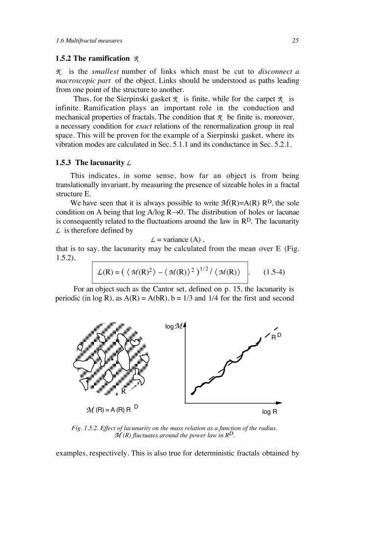
that is to say, the lacunarity may be calculated from the mean over E (Fig.
1.5.2),
L(R) = ( ! M(R)2 " – ! M(R) " 2 )
1/2 / ! M(R) " . (1.5-4)
For an object such as the Cantor set, defined on p. 15, the lacunarity is
periodic (in log R), as A(R) = A(bR), b = 1/3 and 1/4 for the first and second
!
R
(R) = A (R) RM Dlog R
log M
R D
Fig. 1.5.2. Effect of lacunarity on the mass relation as a function of the radius.M (R) fluctuates around the power law in RD.
examples, respectively. This is also true for deterministic fractals obtained by
26 1. Fractal geometries
iterating a generator. The lacunarity becomes aperiodic for random fractals
(Gefen et al., 1983).
1.6 Multifractal measures
Knowledge of the fractal dimension of a set (as we have seen), is
insufficient to characterize its geometry, and, all the more so, any physical
phenomenon occurring on this set. Thus, in a random network of fusible links,
the links which melt are those through the current exceeds a certain threshold.
Their distribution is supported by a set whose fractal dimension generally
differs from that of the whole. Likewise, in a growth phenomenon, such as
diffusion limited aggregation, (the DLA model is described in Sec. 4.2), the
growth sites do not all have the same weight; some of them grow much more
quickly than others. Therefore, to understand many physical phenomena,
involving fractal supports, the (singular) distribution of measures associated
with each point of the support must be characterized. These measures, scalar
quantities, may correspond to concentrations, currents, electrical or chemical
potentials, probabilities of reaching each point of the support, pressures,
dissipations, etc.
Intuitive approach to multifractality
Let us take as an example the distribution of diamonds over the surface of
the earth. We shall suppose that the statistics governing this distribution has
certain similarities with the one in Fig. 1.4.14 (a little too optimistic !): that is,
we suppose that the distribution of diamonds is fractal, that it is not
homogeneous, and that there exist very few regions where large stones occur:
the majority of places on the earth’s surface containing only traces of
diamonds. The information we can draw from knowing the fractal dimension is
global: if it is close to two, diamonds are spread almost uniformly throughout
the world, if it is close to zero, there are a few privileged places where all of the
diamonds are concentrated. In the first situation we soon find something, but
the yield is very low; in the second case we must search for a long time but then
we will be well paid for our efforts. We quickly realize that the information
provided by the fractal dimension is inadequate. There is a measure attached to
the support of this fractal set, which is the price of diamonds as a function of
their volume, clearly it is more worthwhile to find large stones than small ones.
We must use our knowledge of the distribution of diamonds by bringing in the
parameter of their size. Let us suppose that we know the distribution perfectly
(otherwise we must take a sample) and let us cover the globe with a grid,
attaching to each of its square plots of side " the monetary value of the
diamonds found there. To simplify matters the set of plots of land can be
divided into a finite number of batches (i =1,...,N) corresponding to the various
slices of value, from the poorest to the richest [to each plot i we attach in this
1.6 Multifractal measures 27
way its value µ(",xi) relative to the total value]. The correspondence of each of
these batches to a given slice µ specifies a distribution of diamonds on the
earth's surface; we assume that each of these distributions is fractal in the limit
when the side " of the plots tends to zero. The very rare, rich regions will have a
fractal dimension close to zero (“dust”), whereas the regions with only a trace
of diamonds, albeit uniformly distributed, will have a fractal dimension close to
two.
The multifractal character is connected with the heterogeneity of the
distribution (see Sec. 1.4.2, and T.A. Witten in Les Houches, 1987). For a
homogeneous fractal distribution, the mass in the neighborhood of any point in
the distribution is arranged in the same manner. That is to say that inside a
sphere of radius R centered on the fractal at xi, the mass M(R) fluctuates little
about its mean value over all the xi, #M(R)$ whose scaling law is RD: the
distribution P(M) of the masses M(R) taken at different xi is narrow, that is, it
decreases on either side of the mean value faster than any power. In particular,
all the moments vary like #M(R) q $ % #M(R)$ q , for all q. The fractal
distribution is described by the sole exponent D. This is not so for
heterogeneous fractals for which there is a broad distribution, P(M), of the
masses. Such is the case for the distribution of diamonds on the earth’s
surface. Knowledge of the behavior of the moments #M(R) q $ tells us about the
edges of the distribution, namely the very poor and the very rich regions.
We are going to make these ideas sharper using some simple distributions
which will allow us to introduce some mathematical relationships indispensable
in the practical use of the concept of multifractility.
The quantities f(&) and '(q) (which we are now going to define) will allow
us to characterize the distributional heterogeneities of the measures known as
multifractal measures. As these ideas are not initially obvious, the reader may,
if he wishes, turn to the various examples given further on.
1.6.1 Binomial fractal measure
This simple measure is constructed as follows: a segment of length L, on
which a uniform measure of density 1/L is distributed, is divided into two parts
of equal length: l0 = l1= L/2 to which the weights p0 and p1 are given (p0 to the
left and p1 to the right) (Fig. 1.6.1). This process is iterated ad infinitum. The
total measure is preserved if care is taken in choosing
p0 + p1 = 1.
Each element (segment) of the set is labeled by the successive choices (0
left, 1 right) at each iteration. At the nth iteration, each segment is thus indexed
by a sequence [(] ) [(0, (1, …, (k,… (n] where (k = 0 or 1, and has length,
dl = " L = 2 –n L. Its abscissa on the segment E=[0,1] is described simply by
the number in base two
x = l / L = 0. (0(1…(n.
28 1. Fractal geometries
L
L/2
L/2
1
p0
p1
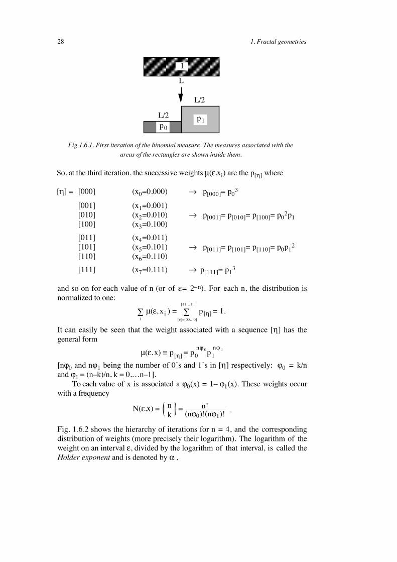
Fig 1.6.1. First iteration of the binomial measure. The measures associated with the
areas of the rectangles are shown inside them.
So, at the third iteration, the successive weights µ(",xi) are the p[(] where
[(] = [000] (x0=0.000) ! p[000]= p03
[001] (x1=0.001)
[010] (x2=0.010) ! p[001]= p[010]= p[100]= p02p1
[100] (x3=0.100)
[011] (x4=0.011)
[101] (x5=0.101) ! p[011]= p[101]= p[110]= p0p12
[110] (x6=0.110)
[111] (x7=0.111) ! p[111]= p13
and so on for each value of n (or of " = 2–n). For each n, the distribution is
normalized to one:
!i
µ(!, x i ) =[11…1]
!["]=[00…0]
p ["] = 1.
It can easily be seen that the weight associated with a sequence [(] has the
general form
µ(!, x) " p [#] = p0n$ 0p1n$ 1
[n*0 and n*1 being the number of 0’s and 1’s in [(] respectively: *0 = k/n
and *1 = (n–k)/n, k = 0,…n–1].
To each value of x is associated a *0(x) = 1– *1(x). These weights occur
with a frequency
N(!,x) = n
k = n!
(n"0)!(n"1)! .
Fig. 1.6.2 shows the hierarchy of iterations for n = 4, and the corresponding
distribution of weights (more precisely their logarithm). The logarithm of the
weight on an interval ", divided by the logarithm of that interval, is called the
Holder exponent and is denoted by & ,
1.6 Multifractal measures 29
! =log µ(")
log "= – #0 log2 p0 – #1 log2 p1
It measures the singular behavior of the measure in the neighborhood of a
point x [via *0(x) and *1(x)], thus
µ(!,x) = !"(x) . (1.6-1)
The values of & are bounded according to the following inequality:
0 < &min= –log2 p0 ! & ! &max= –log2 p1 < ".!
0 1
0 1 10
0 0 0 01 1 1 1
0 0 0 01 1 1 1 0 0 0 01 1 1 1
0 1
x
1001
–logp
20
–logp2
1
!– log
2µ(")
1 2 3 4 5 6 7 8 9 10111213141516
µ (")
= x / "N
("= 1/16)
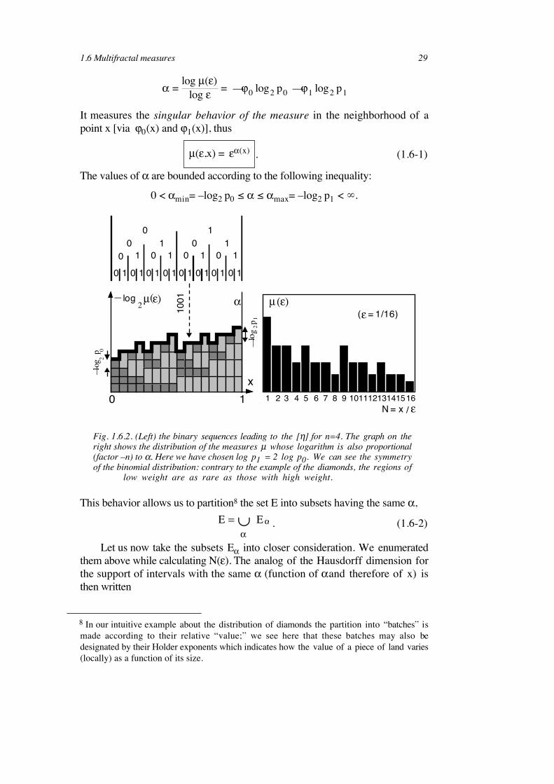
Fig. 1.6.2. (Left) the binary sequences leading to the [(] for n=4. The graph on theright shows the distribution of the measures µ whose logarithm is also proportional(factor –n) to &. Here we have chosen log p1 = 2 log p0. We can see the symmetryof the binomial distribution: contrary to the example of the diamonds, the regions of!!!!!!!!!!!!low weight are as rare as those with high weight.
This behavior allows us to partition8 the set E into subsets having the same &,
! ="#
!#
. (1.6-2)
Let us now take the subsets E& into closer consideration. We enumerated
them above while calculating N("). The analog of the Hausdorff dimension for
the support of intervals with the same & (function of & and therefore of x) is
then written
8 In our intuitive example about the distribution of diamonds the partition into “batches” is
made according to their relative “value;” we see here that these batches may also be
designated by their Holder exponents which indicates how the value of a piece of land varies
(locally) as a function of its size.
30 1. Fractal geometries
!(") = –log N(#,")
log # . (1.6-3)
In the limit of large n (small ") we have simply
! = – log [(n"0)!(n"1)!/n!] / log #
$ – "0 log2"0– "1 log2 "1 .
In the binomial case, this fractal dimension is well defined for each set E&since all the parameters are determined [via *0(x) and *1(x)].
1.6.2 Multinomial fractal measure
The results just shown for a binomial measure easily generalize to
multinomial measures. By considering b weights p+ (0 ! + ! b–1), we can go
through an analogous procedure to that of the binomial measure. Each segment
of size b–n at iteration n is indexed by a sequence [(] or an abscissa x, written
in base b (instead of the 0’s and 1’s of the previous binomial example). The b-
adic intervals are then characterized by the frequencies *+ of their “digits” in
base b. So, the expressions for & and , generalize to
! = – !"
#" logb p" and $ = – !"
#" logb #"
!!"
= 1 !"
p" = 1.with the constraints and"
In the case of a binomial measure (b = 2), , is a single valued function of
&, since two parameters (*0 and *1), whose sum is normalized to one, are used.
For b > 2, this relationship is no longer single valued (there are b–2
supplementary parameters) and the pairs (&,,) cover a certain domain. This
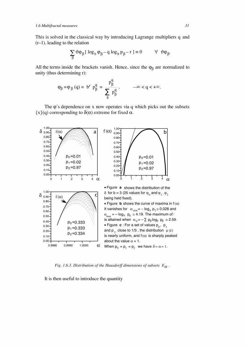
domain is roughly indicated by a network of curves in Fig. 1.6.3 (for b = 3).
The set of [(] (or x expressed in base b) corresponding to the same & is
dominated by the term of highest dimension, f = max , [i.e., by the subset
N(",&) whose exponent , is the greatest]:
N(!,")dominant # !– f(")
. (1.6-4)
This term therefore maximizes
–!!
"! logb "! .
The variation is thus written, (the -*+ then being independent infinitesimal
variables),
! (–!"
#" logb #") $ 0
with the constraints
! = –!"
#" logb p" and 1 = !"
#" .
1.6 Multifractal measures 31
This is solved in the classical way by introducing Lagrange multipliers q and
(r–1), leading to the relation
!!
"#! [ logb #! – q logb p! – r ] $ 0 % "#!.
All the terms inside the brackets vanish. Hence, since the *+ are normalized to
unity (thus determining r):
!" = ! " (q) = br p"
q =
p"
q
!ß
p"
q , – ! < q < +!.
The *’s dependence on x now operates via q which picks out the subsets
{x}(q) corresponding to ,(&) extreme for fixed &.
!
0.028 and
!0 1 2 3 4
f (!) b
!
" f(!) a
0.9980 0.9990 1.0000
f (!)"
!
c
• Figure a shows the distribution of the
" for b!=!3 (25 values for # and # , #
being held fixed).
• Figure b shows the curve of maxima in f
It vanishes for ! = – log p $
! = – log p $ 4.19. The maximum of f
is attained when ! = – " p log p $ 2.59.
• Figure c : For a set of values p , p ,
and p close to 1/3 , the distribution µ (%)
is nearly uniform, and f (!) is sharply peaked
about the value !!= 1.
When p = p = p we have " = ! = 1.
0 1 2
min b 2
max b 0
0 b& &
0 1
2
0 1 2
=
=
p0
p1
p2=
0.01
0.02
0.97
0 1 2 3 4
0.00
0.10
0.20
0.30
0.40
0.50
0.60
0.70
0.80
0.90
1.00
0.00
0.10
0.20
0.30
0.40
0.50
0.60
0.70
0.80
0.90
1.00
=
=
p0
p1
p2=
0.01
0.02
0.97
=
=
p0
p1
p2=
0.333
0.333
0.334
0.00
0.10
0.20
0.30
0.40
0.50
0.60
0.70
0.80
0.90
1.00
(!)
Fig. 1.6.3. Distribution of the Hausdorff dimensions of subsets E& .
It is then useful to introduce the quantity
32 1. Fractal geometries
!(q) = logb!"
p"
q. (1.6-5a)
Very generally '(q) enters in the framework of cumulant generating functions. Note
that some authors have adopted the opposite sign.
& and f(&) are simply related to '(q) by the following relations:
! = –!"
#" logb p" = –$
$qlogb!
"
p"q
and max ! = f(") = – !ß
p#
q [ q logb p# – logb !
ß
p#
q ] / !
ß
p#
q
which reduce to the remarkable equations
! = – "# (q)
"q and f(!) = # (q) – q
"# (q)
"q = # + q! (1.6-5b)
! = –!"
#" logb p" , f(!) = –!"
#" logb #" ,
#" =(p" )
q
!"
(p" )q and $(q) = logb!
"
(p" )q, – " < q < +" .
with
(1.6-5c)
These results (constituting the formalism of multifractals) were obtained
by Frisch and Parisi (1985) and Halsey et al. (1986) using the method of
steepest descent. The concept itself already existed in a 1974 paper of B.
Mandelbrot. Here we have followed the more straightforward approach of B.
Mandelbrot (1988).
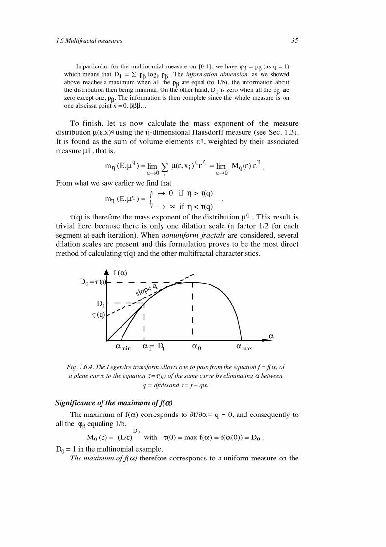
It can be seen that the functions f(&) and '(q) are Legendre transforms of
each other (Fig. 1.6.4). Such transforms are frequently used in
thermodynamics when one wishes to change independent variables.
Formally, f may be compared with an entropy, q with the reciprocal of a
temperature, & with an energy (conjugate variable of q), and ' with a free Gibbs
energy (Lee and Stanley, 1988). The expression for f is indeed that of an
entropy or, more precisely, that of a quantity of information, provided that the
*+ are considered to be the probabilities of finding the measures p+ (the relative
frequences of the digit + in x = 0.(0(1…(n written in base b). The minimum
entropy is obtained when the distribution of the p+ is known exactly, that is,
when one of the *+ = 1 and the others zero (e.g., x = 0.333...33). On the other
hand, the maximum disorder or entropy corresponds to all the *+ being equal
[here the *+ equal 1/b and f(&) = 1]. The expression for *+(q) shows that this
maximum disorder corresponds either to q = 0, or to the trivial case p0 = …
p+ = … pb–1 (= 1/b).
Generally speaking, f(&) is a convex, positive curve, increasing from
1.6 Multifractal measures 33
f(&min) = 0 to a maximum D0 = max f(&), which is equal to one in the previous
example; then f(&) decreases to f(&max) = 0. The extreme values of & are given
simply by the conditions of minimum entropy (one of the *+ = 1, all the rest =
0):
&min = min (–logb p+), &max = max (–logb p+).
Significance of (q)
Consider the following measure:
Mq (!) =!i
µ(!, x i)q
. (1.6-6)
What does this measure represent?
When q = 0, M0(") represents the volume of support measured in
intervals ", M0(") . (L/")D0, with D0 = 1 here, for the segment [0,1] of length L
= 1.
When q = 1, M1(") represents the sum over the support of the measures
on the " intervals. As this measure is normalized,
M1 (!) "[11…1]
![#]=[00…0]
p [#] = 1.
When q! +", Mq is dominated by the regions of high density µ/".When q! –", Mq is dominated by the regions of low density µ/".Thus, the parameter q allows us to select subsets Eq corresponding to
higher or lower densities.
We usually put
Mq (!) = ! (q – 1) Dq ; (1.6-7)
an expression which is true for q = 0 and q = 1. Dq are called qth order
generalized dimensions 9 (the name is due to Hentschel and Procaccia, 1983),
although they are only a dimension when q = 0 (Dq can however be defined as
a critical dimension when q > 1). The advantage of Dq over '(q) resides
essentially in the fact that the former all reduce to the fractal dimension D when
the space is homogeneous, that is,
µ(!,x) " ! D # x,
for then
Mq (!) = !support
µ(!,x )q
" !support
!q D " !– D !q D , and hence Dq = D.
Finally, it can be shown that Dq decreases monotonically as q increases.
We shall now show that (1 – q)Dq = ' (q). From above,
9 Sometimes also called Renyi dimensions.
34 1. Fractal geometries
Mq (!) =!i!q"(x i)
.
Now the number of domains corresponding to the same & is known, it is
N(",&) % " – ,(&), and hence
Mq (!) "
#min
#max
d# !q # – $(#).
This integral is dominated by the maxima of ,(&) with the value of & which
minimizes the exponent (" « 1), that is, &(q) such that
!
!"
[q " – max #(")]"="(q)= 0, max #(")
"="(q) $ f("(q))where
which agrees with the earlier results. By comparison it can be seen that Mq(")% " q & – f , hence
Mq (!) " !# $(q)
$(q) = (1– q) Dq = – lim!%0
1log !
log!i
µ(!,x i )q
with . (1.6-8)
(The integral is a discrete sum if the box method is used.)
Form and meaning of D1
When q = 1, the above expression is undetermined. So what is the form
and the meaning of D1, the first order generalized dimension? For this we must
calculate
D1 = limq!1
1q–1
lim"!0
log Mq (")
log ". (1.6-9)
Writing [µ(",x)q ] = (µ µq – 1 ) / µ[1+ (q–1) log µ], so that
log Mq (!) = log!i
µ(!,x i )q" log !
i1+ (q–1)µ(!,x i )log µ(!,x i
" (q–1)!i
µ(!,x i )log µ(!,x i )
[ )]
gives D1 = lim!"0
1log !
!i
µ (!,xi ) log µ (!,xi ) . (1.6-10)
Moreover, we can relate this expression to & and f(&) by differentiating '(q).
We then find that
D1 = & q = 1 = f (& q = 1) . (1.6-11)
The remarkable property of D1 comes from the fact that # µ(") log µ(")
represents the entropy of information of the distribution whose scale behavior
D1 describes. For this reason D1 is called the information dimension. The
support set E&(1) contains almost all the measure (or mass) of the set E.
1.6 Multifractal measures 35
In particular, for the multinomial measure on [0,1], we have *+ = p+ (as q = 1)
which means that D1 = # p+ logb p+. The information dimension, as we showed
above, reaches a maximum when all the p+ are equal (to 1/b), the information about
the distribution then being minimal. On the other hand, D1 is zero when all the p+ are
zero except one, p+. The information is then complete since the whole measure is on
one abscissa point x = 0. +++…
To finish, let us now calculate the mass exponent of the measure
distribution µ(",x)q using the (-dimensional Hausdorff measure (see Sec. 1.3).
It is found as the sum of volume elements "(, weighted by their associated
measure µq , that is,
m! (",µq) = lim
#$0!i
µ(#, x i )q#!= lim
#$0Mq (#) #
!
.
From what we saw earlier we find that
m! (",µq ) = # 0 if ! > $(q)
# ! if ! < $(q).
'(q) is therefore the mass exponent of the distribution µq . This result is
trivial here because there is only one dilation scale (a factor 1/2 for each
segment at each iteration). When nonuniform fractals are considered, several
dilation scales are present and this formulation proves to be the most direct
method of calculating '(q) and the other multifractal characteristics.
!
!f )(
" (q)
D0 =
! 0!min !max
D1
! = D1 1
" (0)
slope q
Fig. 1.6.4. The Legendre transform allows one to pass from the equation f = f(&) of
a plane curve to the equation ' = '(q) of the same curve by eliminating & between
q = df/d& and ' =!f – q&.
Significance of the maximum of f( )
The maximum of f(&) corresponds to $f/$& ) q = 0, and consequently to
all the *+ equaling 1/b,
M0 (!) = (L/!)D0
"(0) = max f(#) = f(#(0)) = D0 .with
D0 = 1 in the multinomial example.
The maximum of f(&) therefore corresponds to a uniform measure on the
36 1. Fractal geometries
support. Its value is thus the dimension (fractal or otherwise) of the support.
Here, it is that of a segment [0, L] and therefore equals one.
Everything that has been developed for the multinomial case will contribute
to understanding the general case of a distribution of measures over a fractal
support. We shall approach this subject by explaining in detail two important
measures for physics, the multifractal measure of a distribution of points, mass
or current (developed turbulence, strange attractors, distributions of galaxies or
flux of matter in a porous rock, resistors networks), and the harmonic
multifractal measure (growth phenomena, DLA, etc.). Remaining within the
general framework, some structures which are fractal on several scales, with
multifractal characteristics which may be fully calculated, will be considered.
1.6.3 Two-scale Cantor sets
The Cantor sets mentioned in Sec. 1.4.1 with their uniform measures are
not multifractal; in fact their curves f(&) reduce to a point [& = f(&) = D]. They
are pure fractals. To generate a multifractal structure with a uniform measure at
least two dilation scales must be used.
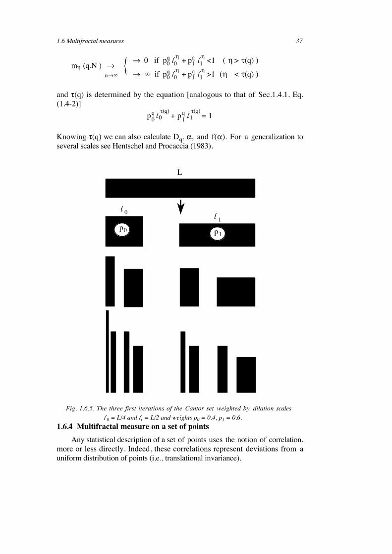
Let us examine one of these structures by treating the general case: two
measure scales, two dilation scales. The following structure (Cantor bars)
generalizes the binomial measure studied above. An initial segment of length L
and unit measure (mass) is divided into two parts: l0 and l1 to which we
associate the measures p0 and p1 (p0 + p1 = 1). The first three steps of the
construction are shown in Fig. 1.6.5.
Determination of (q)
'(q) will be determined by calculating the (-dimensional Hausdorff
measure. In practice the result is completely analogous to that giving the fractal
dimension calculated from Eq. 1.4-2. We therefore calculate
m! (q,N ) =
N–1
!i=0
µiq li
! = "
#"0
" 0 if ! > $(q)
" " if ! < $(q) where # = max (l i ) .
In the present case, i = [0, N–1] designates the i th element out of N = 2n, (n
being the number of iterations). It takes the place of x in the binomial measure.
The measure and the size of the i th element are, respectively,
µi = p0 k p1
n!– !k and l i = l 0 k l 1
n!– !k
and its degeneracy is the number of ways of choosing k objects out of n
without regard to order of choice. Thus,
m! (q,N ) = !k=0
n
n
k (p0
k p1 n–k )q ( l 0
k l 1 n–k
)!
= p0q l0
! + p1
q l1 ! n
1.6 Multifractal measures 37
m! (q,N ) "
n"!
" 0 if p0q l0
! + p1
q l1 !
<1 ( ! > #(q) )
" ! if p0q l0
! + p1
q l1 !
>1 ( ! < #(q) )
and '(q) is determined by the equation [analogous to that of Sec.1.4.1, Eq.
(1.4-2)]
p0q l0
!(q)+ p
1q l1
!(q)= 1
Knowing '(q) we can also calculate Dq, &, and f(&). For a generalization to
several scales see Hentschel and Procaccia (1983).
L
p0 p1
l0
l1
Fig. 1.6.5. The three first iterations of the Cantor set weighted by dilation scales
! ! ! ! ! ! ! ! ! ! ! ! l 0 !=!L/4 and l1 = L/2 and weights p0 = 0.4, p1 = 0.6.
1.6.4 Multifractal measure on a set of points
Any statistical description of a set of points uses the notion of correlation,
more or less directly. Indeed, these correlations represent deviations from a
uniform distribution of points (i.e., translational invariance).
38 1. Fractal geometries
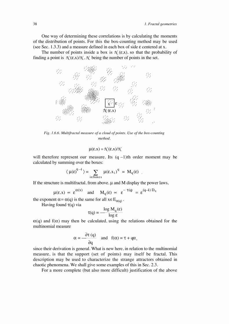
One way of determining these correlations is by calculating the moments
of the distribution of points. For this the box-counting method may be used
(see Sec. 1.3.3) and a measure defined in each box of side " centered at x.
The number of points inside a box is N (",x), so that the probability of
finding a point is N (",x)/N , N being the number of points in the set.
x !
N (!,x)
Fig. 1.6.6. Multifractal measure of a cloud of points. Use of the box-counting
method.
µ(",x) = N (",x)/N
will therefore represent our measure. Its (q –1)th order moment may be
calculated by summing over the boxes:
! µ(")q –1
# = !i$boxes
µ(",x i )q= Mq (") .
If the structure is multifractal, from above, µ and M display the power laws,
µ(!,x) " !#(x)
Mq (!) " !$ %(q)
= !(q–1) Dq
and
the exponent & = &(q) is the same for all x0E&(q) .
Having found '(q) via
!(q) = –log Mq (")
log "
&(q) and f(&) may then be calculated, using the relations obtained for the
multinomial measure
! = – "# (q)
"q and f(!) = # + q!,
since their derivation is general. What is new here, in relation to the multinomial
measure, is that the support (set of points) may itself be fractal. This
description may be used to characterize the strange attractors obtained in
chaotic phenomena. We shall give some examples of this in Sec. 2.3.
For a more complete (but also more difficult) justification of the above

1.6 Multifractal measures 39
formalism, Collet et al. (1987), Bohr and Rand (1987), Rand (1989), and Ruelle
(1982, 1989) may be consulted.
40 1. Fractal geometries

![A Research Paper - University of Technology, Iraq of... · 2018-01-19 · multiband can be achieved through using different techniques like fractals [2]. Fractal geometries are characterized](https://img.dokumen.tips/doc/110x75/5f6e3488e784b336201c0a8d/a-research-paper-university-of-technology-iraq-of-2018-01-19-multiband.jpg)