Contribution of the Hanbury Brown – Twiss experiment to thedevelopment of quantum optics

Kis Zsolt

Kvantumoptikai és Kvantuminformatikai OsztályMTA Wigner Fizikai Kutatóközpont

H-1121 Budapest, Konkoly-Thege Miklós út 29-33

BME, 2013. május 15.

Table of contents

First- and second-order coherence of lightClassical interference of lightThe Hanbury Brown – Twiss experimentsRoy J. Glauber: the quantum theory of optical coherence

ApplicationsExperimental test of the Bell’s inequalityQuantum state reconstruction of lightContinuous variable quantum key distribution

Table of contents

First- and second-order coherence of lightClassical interference of lightThe Hanbury Brown – Twiss experimentsRoy J. Glauber: the quantum theory of optical coherence

ApplicationsExperimental test of the Bell’s inequalityQuantum state reconstruction of lightContinuous variable quantum key distribution

Light interference on a screen

I Electric field strength (complex analytic signal):

E(r , t) = |E(r , t)|eiφ(r,t)

I In general E(r , t) is a wave packet:

E(r , t) =

∫dωE(ω)ei(k r−ωt)

The intensity distribution on the screen:

I =12

(|E(r , t)|2 + |E(r , t + ω0L/c)|2 + Re{E(r , t)∗E(r , t + ω0L/c)}

)For plane waves (E = E0ei(kr−ωt))

I =I02

(1 + cos(ωL/c))

First order coherenceg(1)(τ) =

〈E(r , t)∗E(r , t + τ)〉〈E(r , t)∗E(r , t)〉 ,

where 〈...〉 means manifold or time average (ergodicity).

Measuring the angular diamater of a star

Spatial coherence of a wave front (astronomical Michelson in-terferometer):

I =12〈[E(r1) + E(r2)]∗[E(r1) + E(r2)]〉

=12

(⟨|E(r1)|2

⟩+⟨|E(r2)|2

⟩+ 2Re{E(r1)∗E(r2)}

)= 2I0

(1 + g(1)(r1, r2)

)

For two wave fronts:

I =12

⟨|Ek (r1) + Ek ′(r1) + Ek (r2) + Ek ′(r2)|2

⟩= 4I0(1 + cos([k + k ′]d/2) cos(kdφ/2)) ,

where d = r1 − r2. The term cos(kdφ/2) depends on the angular diameter φ of thestar.

Drawback: the method has large uncertainty due to cos([k + k ′]d/2)

The Hanbury Brown – Twiss effect (1956)What is the intensity correlation between different points of the wavefront?

C(d) =〈∆J1(t)∆J2(t)〉

〈(∆J1(t))2〉1/2〈(∆J2(t))2〉1/2

What do we observe in the light intensitycorrelation experiment?

Answer: correlation of photocurrents!

Emission of photoelectronsThe Hamiltonian of the detector reads

H = εg |g〉〈g|+∑

q

εe,q |e, q〉〈e, q| −∑

q

[µ(eq),g |e, q〉〈g|+ H.c.](E(t) + E∗(t))

The state vector is defined as: |ψ〉 = cg |g〉+∑

q ce,q |e, q〉The Schrödinger equation for the state vector in the interaction picture

iddt

cg = −∑

q

∫ ∞0

dωµ∗(eq),gE∗(ω)

~e−i(ωq−ω)tce,q

iddt

ce,q = −∫ ∞

0dω

µ(eq),gE(ω)

~ei(ωq−ω)tcg

where ~ωq = εe,q − εg , {cg(t0) = 1, ce,q(t0) = 0}Apply the time-dependent perturbation theory, and compute ce,q(t), (t = t0 + ∆t)

ce,q(t) =i∆t~

∫dωµ(eq),gE(ω)ei(ωq−ω)(t0+∆t/2)

sin(ωq−ω

2 ∆t)

ωq−ω2 ∆t

The total transition probability per unit time to the excited state ((ω − ω′)∆t � 1)

Π(t) =1

∆t

∑q

|ce,q(t)|2 ≈ 1∆t

∫ ∞0

dωq |ce,q(t)|2%(ωq)

Emission of photoelectrons (cont.)

The probability of emitting a single photoelectron in the ∆t interval (∝ Fermi g.r.)

P(1, t , t + ∆t) = 2π%(ω0)

~2 |µ(ek0),g |2 · I(t) ·∆t ≡ ηI(t)∆t

where I(t) = |E(t)|2, E(t) =∫

dωE(ω) exp(−iωt), k0 = ω0/c0

If there are N effective emitters

P(?, t , t + ∆t) =N∑1

(Nn

)[ηI(t)∆t ]n[1− ηI(t)∆t ]N−n = 1− [1− ηI(t)∆t ]N

= NηI(t)∆t − N(N − 1)

2![ηI(t)∆t ]2 + . . .

For ηI(t)∆t � 1P(1, t , t + ∆t) = NηI(t)∆t ≡ ηI(t)∆t

The probability of emitting n photoelectrons in [t , t + T ], assuming independentemissions, follows the Poisson distribution

P(n, t , t + T ) =[ηU(t ,T )]n

n!exp(−ηU(t ,T ))

with U(t ,T ) =∫ t+T

t dτ I(τ) the fluence

Properties of the P(n, t , t + T ) distribution

Mean number of emitted photoelectrons:

〈n〉 = η

∫ t+T

tdτ I(τ)

Mean photoelectron number from P(n, t , t + T )

〈n〉 =∞∑

n=0

n P(n, t , t + T ) = ηU(t ,T ) = η

∫ t+T

tdτ I(τ)

Calculating the variance of the photoelectron number

〈n2〉 =∞∑

n=0

[n(n − 1) + n] P(n, t , t + T ) = [ηU(t ,T )]2 + ηU(t ,T )

〈(n − 〈n〉)2〉 = 〈n2〉 − 〈n〉2 = [ηU(t ,T )]2 + ηU(t ,T )− [ηU(t ,T )]2 = ηU(t ,T )

∆n =√ηU(t ,T )

Fluctuating classical fieldsThe quantity ηU(t ,T ) is a random variable W −→ ensemble averaging is necessary

f (W ) : probability distribution∫ ∞0

f (W )dW = 1

P(n, t , t + T ) =

⟨W n

n!exp(−W )

⟩=

∫dW f (W )

W n

n!exp(−W )

〈n〉 = 〈W 〉〈(n − 〈n〉)2〉 = 〈W 〉+ 〈(∆W )2〉

For T � τc , τc is the correlation time of I(t)

W = η〈I〉T , ergodic process

P(n, t , t + T ) =[η〈I〉T ]n

n!exp(−η〈I〉T )

For T � τc , I(t) is nearly constant in [t , t + T ]

W = ηI(t)T

P(n, t , t + T ) =

∫dI f (I)

[ηIT ]n

n!exp(−ηIT )

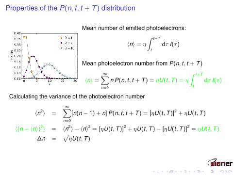
Fluctuating classical fields (cont.)

Example: classical thermal field

p(E)d2E =1

2π〈I〉 exp(−|E |2/〈I〉)dI · dϕ

P(I) =1〈I〉 exp(−I/〈I〉)

P(n, t , t + T ) =(1 + η〈I〉T )n

(1 + η〈I〉T )n+1

Boson statistics for the photoelectrons ...

Joint detection by two independent photodetectors:

Π1(r1, t1)∆t1 = η1I(r1, t1)∆t1Π1(r2, t2)∆t2 = η2I(r2, t2)∆t2

P{1}(r1, t1; r2, t2)∆t1∆t2 = η1η2I(r1, t1)I(r2, t2)∆t1∆t2

For fluctuating fields

P{1}(r1, t1; r2, t2)∆t1∆t2 = η1η2〈I(r1, t1)I(r2, t2)〉∆t1∆t2

Photoelectric current fluctuation

Usually the current of the electrons of the detector is amplified −→ current pulsesThe current pulses are not always resolved −→ a continuous current J(t) is studied

J(t) =∑

r

s(t − tr )

Let’s assume that n photoelectrons are emitted in time T . In a stationary field theaverage current is (emission prob. = dtr/T )

〈Jn,T (t)〉n =n∑

r=1

∫ T

0s(t − tr )

dtrT

=1T

n∑r=1

∫s(t − tr )dt ≈ 1

T

n∑r=1

Q =nQT

The average current

〈J(t)〉 =∞∑

n=0

P(n, t , t + T )nQT

= 〈n〉QT

= η〈n〉Q

Photoelectric current correlation

Autocorrelation (TR � T )

〈∆J(t)∆J(t + τ)〉 = η〈I〉∫ ∞−∞

s(t ′)s(t ′ + τ)dt ′

+ η2∫∫ ∞−∞

s(t ′)s(t ′′)〈∆I(t)∆I(t + t ′ − t ′′ + τ)〉dt ′dt ′′

For slow response photodetector (τc � TR)

〈∆J(t)∆J(t + τ)〉 =[η〈I〉+ η2〈(∆I)2〉τc

] ∫ ∞−∞

s(t ′)s(t ′ + τ)dt ′

Cross-correlation

〈∆J1(t)∆J2(t + τ)〉 = η1η2

∫∫ ∞−∞

s(t ′)s(t ′′)〈∆I1(t)∆I2(t + t ′ − t ′′ + τ)〉dt ′dt ′′

For slow response photodetector

〈∆J1(t)∆J2(t + τ)〉 = η1η2〈∆I1∆I2〉τc

∫ ∞−∞

s(t ′)s(t ′ + τ)dt ′

Explanation of the original HBT effectReacall : the normalized intensity correlation between two points of the wavefront

C(d) =〈∆J1(t)∆J2(t)〉

〈(∆J1(t))2〉1/2〈(∆J2(t))2〉1/2

The autocorrelation is given by

〈(∆Ji (t))2〉 = ηi

[〈Ii〉+ ηi〈(∆Ii )2〉τc

] ∫ ∞−∞

s2(t ′)dt ′

For unpolarized thermal field 〈(∆I)2〉 = 12 〈I〉

2

〈(∆Ji (t))2〉 = ηi〈Ii〉[1 +

12ηi〈Ii〉τc

] ∫ ∞−∞

s2(t ′)dt ′

The cross cross correlation

〈∆J1(t)∆J2(t)〉 = η1η2〈∆I1∆I2〉τc

∫ ∞−∞

s2(t ′)dt ′

Using the relation 〈z∗1 z1z∗2 z2〉 = 〈z∗1 z1〉〈z∗2 z2〉+ 〈z∗2 z1〉〈z∗1 z2〉 (zi Gaussian)

〈∆J1(t)∆J2(t)〉 =12η1η2〈I1〉〈I2〉τc |γ(r1, r2, 0)|2

∫ ∞−∞

s2(t ′)dt ′

Measuring the diameter of a star

Let’s measure the normalized second order current correlation:

C(d) =〈∆J1(t)∆J2(t)〉

〈(∆J1(t))2〉1/2〈(∆J2(t))2〉1/2 = η〈I〉τc [1 + cos(k d φ)]

〈(∆Ji (t))2〉 = ηi〈Ii〉[1 +

12ηi〈Ii〉τc

] ∫ ∞−∞

s2(t ′)dt ′

〈∆J1(t)∆J2(t)〉 =12η1η2〈∆I1∆I2〉τc

∫ ∞−∞

s2(t ′)dt ′

In case of two wave fronts:

〈∆I1∆I2〉 = 〈E(r1)∗E(r2)∗E(r1)E(r2)〉 − 〈E(r1)∗E(r1)〉〈E(r2)∗E(r2)〉= 〈[Ek + Ek′ ]∗(r1)[Ek + Ek′ ]∗(r2)[Ek + Ek′ ](r2)[Ek + Ek′ ](r1)〉− 〈[Ek + Ek′ ]∗(r1)[Ek + Ek′ ](r1)〉〈[Ek + Ek′ ]∗(r2)[Ek + Ek′ ](r2)〉

= 2⟨|Ek |2|Ek ′ |2

⟩+{⟨

E∗k Ek E∗k′ Ek′

⟩ei(k−k′)(r2−r1) + c.c.

}= 2 〈Ik 〉〈Ik ′〉 [1 + cos(k d φ)]

Second order correlation function of quantized fieldsElectric field operator for 1D, polarized e.m. field

E(z) = E (+) + E (−) = i∑

k

[√~

2ωε0Laeikz + H.c.

]

where E (+) ∼ E(t) classical

Intensity : I = 〈E (−)(r)E (+)(r)〉

Second order correlation function:

G(2) = 〈: E (−)(r1)E (+)(r1)E (−)(r2)E (+)(r2) :〉 ≡ 〈E (−)(r1)E (−)(r2)E (+)(r2)E (+)(r1)〉

where [: a†a a†a :] = a†a† a a

Stellar interferometer: assume 〈nk 〉 = 〈nk′〉 ≡ 〈n〉, furthermore 〈n2k 〉 = 〈n2

k′〉 ≡ 〈n2〉

G(2) = 2E4(〈n2〉 − 〈n〉+ 〈n〉2

{1 + cos[(k − k ′)(r1 − r2)]

})light source G(2) min max

thermal 2n2 + n2(1 + χ) 2n2 4n2

laser n2 + n2(1 + χ) n2 3n2

single photon 1 + χ 0 2

where n = 〈n〉, χ = cos[(k − k ′)(r1 − r2)]

Observation of correlations through photon counting

Counting rates

PT (0,T ) = RT (0,T )∆t =

(NT (0,T )

∆T

)∆t

PR(τ,T ) = RR(τ,T )∆t =

(NR(τ,T )

∆T

)∆t

PTR(τ,T ) = RTR(τ,T )∆t =

(NTR(τ,T )

∆T

)∆t

Correlation between photo-counts (mode V is in vacuum)

g(2)T ,R(τ) =

〈: IT (0)IR(τ) :〉〈IT (0)〉〈IR(τ)〉

, g(2)T ,R(0) =

〈a†T a†R aT aR〉〈a†T aT 〉〈a†R aR〉

=〈nI(nI − 1)〉〈nI〉2

where

aR =aI + aV√

2, aT =

aI − aV√2

Some measurements (by Krisztián Lengyel)The probabilty distribution P(n, t , t + T ) for laser light

0

20

40

60

80

100

120

140

160

180

200

0 1 2 3 4 5 6 7 8 9 10 11 12 13 14 15 16 17 18 19 20 21

Nin

t [db

]

Nphoton [db]

λ = 7.62 ± 0.06tint=5 µs

here T = 5µs, detector pulse length ≈ 18ns, detector dead time ≈ 40ns,sampling time bin = 400ps

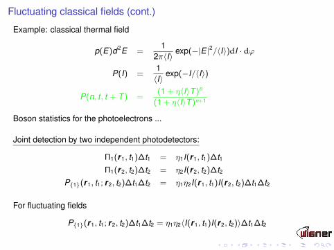
Some measurements (cont.)

Hanbury Brown–Twiss effect from photon counting

0 1 2 3 4

Ude

t

t [µs]

AC

A*C

Some measurements (cont.)

There are no quantum effects here

0

0.02

0.04

0.06

0.08

0.1

0.12

0.14

0 1 2 3 4

I AB

IA*IB

LaserSpectral lamp

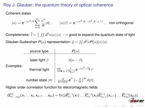
Roy J. Glauber: the quantum theory of optical coherence

Coherent states

|α〉 = e−|α|2/2

∞∑n=0

αn

n!|n〉 , 〈α|β〉 = e−|α|

2/2−|β|2/2−α∗β , non-orthogonal

Completeness: I = 1π

∫∫d2α|α〉〈α| −→ good to expand the quantum state of light

Glauber-Sudarshan P(α) representation: % =∫∫

d2αP(α)|α〉〈α|

Examples:

source type P(α)

laser light β δ(α− β)

thermal light∏

k ,s1

π〈nk,s〉e−|α|

2/〈nk,s〉

number state |n〉 n!2πr(2n)!

er2 (− ∂∂r

)2nδ(r)

Higher order correlation function for electromagnetic fields

G(n)µ1...µ2n (x1 . . . xn, xn+1 . . . x2n) = Tr{%E (−)

µ1 (x1) . . . E (−)µn (xn)E (+)

µn+1 (xn+1) . . . E (+)µ2n (x2n)}

Table of contents

First- and second-order coherence of lightClassical interference of lightThe Hanbury Brown – Twiss experimentsRoy J. Glauber: the quantum theory of optical coherence

ApplicationsExperimental test of the Bell’s inequalityQuantum state reconstruction of lightContinuous variable quantum key distribution

The Hong-Ou-Mandel interferometer

Interference of single-photon wave packetsI Two photons impinge at the two

imputs of the beam splitter: |1a, 1b〉I Passing the beam splitter

(R = T = 50%) the photons „sticktogether”:

|ψout〉 =i√2

(|2A, 0B〉+ |0A, 2B〉)

The coincidence tends to zero if the twophotons arrive at the same time to thebeam splitter.

Design of single photon wave packets

I Single photons source with an atom trapped inside a cavity: the atom isperiodically excited (T = 3µs), to get a stream of photons

I G(2) = 〈PD1(t)PD2(t − τ)〉 is measured in a HBT setup to prove the singlephoton state

I A Hong-Ou-Mandel interferometer is used to test the overlap between thephoton wave packets.

Experimental test of the Bell’s inequalityEinstein’s locality: the outcome of a measurement cannot depend on parameterscontrolled by faraway agents.

Two observers test the polarization of photons emitted in an S P S cascade.

Observer A measures α, γ polarizations, the outcome ±1.Observer B measures β, δ polarizations, the outcome ±1.

If local hidden variables exist (Clauser, Horne, Shimony, Holt)

ajbj + bjcj + cjdj − djaj ≡ ±2

After averaging

| cos 2(α− β) + cos 2(β − γ) + cos 2(γ − δ)− cos 2(δ − α)| ≤ 2

QM says: lhs = 2√

2, agrees with the measurement

Quantum state reconstruction of light

Quantum state reconstruction: find the density operator % . . . or something equivalent

Quasiprobability distributions:I Glauber-Sudarshan P(α) representation : not good, it’s an ugly distributionI Wigner’s function, W (q, p) = 1

2π

∫∞−∞ exp(ipx)〈q − x/2|%|q + x/2〉dx

I The Q(α) function : Q(α) = 〈α|%|α〉

How to reconstruct the phase space dis-tributions ?

Measure the quadrature distributions:

qθ = q cos θ + p sin θ

From the marginal distributions pr(q, θ) a quasiprobability distribution between Wand Q can be reconstructed.

Homodyne detection for measuring pr(q, θ)

There are two fields: 1. signal; 2. the localoscillator

Very important: they are phase locked

Beam splitter mixing:

a′1 =a + αLO√

2

a′2 =a− αLO√

2

Measure the intensity at the output ports:

I1 =12{〈a†a〉+|αLO|2+|αLO|(ae−iθ+a†eiθ)} , I2 =

12{〈a†a〉+|αLO|2−|αLO|(ae−iθ+a†eiθ)}

Record the difference

I1 − I2 = |αLO|(ae−iθ + a†eiθ) ≈ qθ

Continuous variable quantum key distribution

Thank you for your attention