Continuous-Time Mean–Variance Portfolio

Selection: A Reinforcement Learning Framework∗

Haoran Wang† Xun Yu Zhou‡

First draft: February 2019This version: May 2019

Abstract

We approach the continuous-time mean–variance (MV) portfolioselection with reinforcement learning (RL). The problem is to achievethe best tradeoff between exploration and exploitation, and is formu-lated as an entropy-regularized, relaxed stochastic control problem.We prove that the optimal feedback policy for this problem must beGaussian, with time-decaying variance. We then establish connectionsbetween the entropy-regularized MV and the classical MV, includingthe solvability equivalence and the convergence as exploration weight-ing parameter decays to zero. Finally, we prove a policy improvementtheorem, based on which we devise an implementable and data-drivenRL algorithm. We find that our algorithm outperforms both an adap-tive control based method and a deep neural networks based algorithmby a large margin in our simulations.

Key words. Reinforcement learning, mean-variance portfolio se-lection, entropy regularization, stochastic control, value function, Gaus-sian distribution, policy improvement theorem.

∗We are grateful for comments from the seminar participants at the Fields Institute.Wang gratefully acknowledges financial supports through the FDT Center for IntelligentAsset Management at Columbia. Zhou gratefully acknowledges financial supports througha start-up grant at Columbia University and through the FDT Center for Intelligent AssetManagement.†Department of Industrial Engineering and Operations Research, Columbia University,

New York, NY 10027, USA. Email: hw2718@columbia.edu.‡Department of Industrial Engineering and Operations Research, and The Data Science

Institute, Columbia University, New York, NY 10027, USA. Email: xz2574@columbia.edu.

1

1 Introduction

Applications of reinforcement learning (RL) to quantitative finance (e.g.,algorithmic and high frequency trading, smart order routing, portfolio man-agement, etc) have attracted more attentions in recent years. One of themain reasons is that the electronic markets prevailing nowadays can providesufficient amount of microstructure data for training and adaptive learning,much beyond what human traders and portfolio managers could handle inold days. Numerous studies have been carried out along this direction. Forexample, Nevmyvaka et al. (2006) conducted the first large scale empiri-cal analysis of RL method applied to optimal order execution and achievedsubstantial improvement relative to the baseline strategies. Hendricks andWilcox (2014) improved over the theoretical optimal trading strategies ofthe Almgren-Chriss model (Almgren and Chriss (2001)) using RL techniquesand market attributes. Moody and Saffell (2001) and Moody et al. (1998)studied portfolio allocation problems with transaction costs via direct policysearch based RL methods, without resorting to forecast models that rely onsupervised leaning.

However, most existing works only focus on RL optimization problemswith expected utility of discounted rewards. Such criteria are either un-able to fully characterize the uncertainty of the decision making process infinancial markets or opaque to typical investors. On the other hand, mean–variance (MV) is one of the most important criteria for portfolio choice.Initiated in the seminal work Markowitz (1952) for portfolio selection ina single period, such a criterion yields an asset allocation strategy thatminimizes the variance of the final payoff while targeting some prespecifiedmean return. The MV problem has been further investigated in the discrete-time multiperiod setting (Li and Ng (2000)) and the continuous-time setting(Zhou and Li (2000)), along with hedging (Duffie and Richardson (1991))and optimal liquidation (Almgren and Chriss (2001)), among many othervariants and generalizations. The popularity of the MV criterion is not onlydue to its intuitive and transparent nature in capturing the tradeoff betweenrisk and reward for practitioners, but also due to the theoretically interest-ing issue of time-inconsistency (or Bellman’s inconsistency) inherent withthe underlying stochastic optimization and control problems.

From the RL perspective, it is computationally challenging to seek theglobal optimum for Markov Decision Process (MDP) problems under the MVcriterion (Mannor and Tsitsiklis (2013)). In fact, variance estimation andcontrol are not as direct as optimizing the expected reward-to-go which hasbeen well understood in the classical MDP framework for most RL problems.

2

Because most standard MDP performance criteria are linear in expectation,including the discounted sum of rewards and the long-run average reward(Sutton and Barto (2018)), Bellman’s consistency equation can be easilyderived for guiding policy evaluation and control, leading to many state-of-the-art RL techniques (e.g., Q-learning, temproaral difference (TD) learning,etc). The variance of reward-to-go, however, is nonlinear in expectation and,as a result, most of the well-known learning rules cannot be applied directly.

Existing works on variance estimation and control generally divide intotwo groups, value based methods and policy based methods. Sobel (1982)obtained the Bellman’s equation for the variance of reward-to-go under afixed, given policy. Based on that equation, Sato et al. (2001) derived theTD(0) learning rule to estimate the variance under any given policy. In arelated paper, Sato and Kobayashi (2000) applied this value based methodto an MV portfolio selection problem. It is worth noting that due to theirdefinition of the intermediate value function (i.e., the variance penalizedexpected reward-to-go), Bellman’s optimality principle does not hold. As aresult, it is not guaranteed that a greedy policy based on the latest updatedvalue function will eventually lead to the true global optimal policy. Thesecond approach, the policy based RL, was proposed in Tamar et al. (2013).They also extended the work to linear function approximators and devisedactor-critic algorithms for MV optimization problems for which convergenceto the local optimum is guaranteed with probability one (Tamar and Mannor(2013)). Related works following this line of research include Prashanth andGhavamzadeh (2013, 2016), among others. Despite the various methodsmentioned above, it remains an open and interesting question in RL tosearch for the global optimum under the MV criterion.

In this paper, we establish an RL framework for studying the continuous-time MV portfolio selection, with continuous portfolio (control/action) andwealth (state/feature) spaces. The continuous-time formulation is appealingwhen the rebalancing of portfolios can take place at ultra-high frequency.Such a formulation may also benefit from the large amount of tick data thatis available in most electronic markets nowadays. The classical continuous-time MV portfolio model is a spacial instance of a stochastic linear–quadratic(LQ) control problem (Zhou and Li (2000)). Recently, Wang et al. (2019)proposed and developed a general entropy-regularized, relaxed stochasticcontrol formulation, called an exploratory formulation, to capture explic-itly the tradeoff between exploration and exploitation in RL. They showedthat the optimal distributions of the exploratory control policies must beGaussian for an LQ control problem in the infinite time horizon, therebyproviding an interpretation for the Guassian exploration broadly used both

3

in RL algorithm design and in practice.While being essentially an LQ control problem, the MV portfolio selec-

tion must be formulated in a finite time horizon which is not covered byWang et al. (2019). The first contribution of this paper is to present theglobal optimal solution to the exploratory MV problem. One of the interest-ing findings is that, unlike its infinite horizon counterpart derived in Wanget al. (2019), the optimal feedback control policy for the finite horizon caseis a Gaussian distribution with a time-decaying variance. This suggests thatthe level of exploration decreases as the time approaches the end of theplanning horizon. On the other hand, we will obtain results and observeinsights that are parallel to those in Wang et al. (2019), such as the perfectseparation between exploitation and exploration in the mean and varianceof the optimal Gaussian distribution, the positive effect of a random envi-ronment on learning, and the close connections between the classical andthe exploratory MV problems.

The main contribution of the paper, however, is to design an inter-pretable and implementable RL algorithm to learn the global optimal so-lution of the exploratory MV problem, premised upon a provable policyimprovement theorem for continuous-time stochastic control problems withboth entropy regularization and control relaxation. This theorem providesan explicit updating scheme for the feedback Gaussian policy, based on thevalue function of the current policy in an iterative manner. Moreover, itenables us to reduce from a family of general non-parametric policies to aspecifically parametrized Gaussian family for exploration and exploitation,irrespective of the choice of an initial policy. This, together with a care-fully chosen initial Gaussian policy at the beginning of the learning process,guarantees the fast convergence of both the policy and the value function tothe global optimum of the exploratory MV problem.

We further compare our RL algorithm with two other methods applied tothe MV portfolio optimization. The first one is an adaptive control approachthat adopts the real-time maximum likelihood estimation of the underlyingmodel parameters. The other one is a recently developed continuous con-trol RL algorithm, a deep deterministic policy gradient method (Lillicrapet al. (2016)) that employs deep neural networks. The comparisons are per-formed under various simulated market scenarios, including those with bothstationary and non-stationary investment opportunities. In nearly all thesimulations, our RL algorithm outperforms the other two methods by a largemargin, in terms of both performance and training time.

The rest of the paper is organized as follows. In Section 2, we presentthe continuous-time exploratory MV problem under the entropy-regularized

4

relaxed stochastic control framework. Section 3 provides the complete solu-tion of the exploratory MV problem, along with connections to its classicalcounterpart. We then provide the policy improvement theorem and a con-vergence result for the learning problem in Section 4, based on which wedevise the RL algorithm for solving the exploratory MV problem. In Sec-tion 5, we compare our algorithm with two other methods in simulationsunder various market scenarios. Finally, we conclude in Section 6.

2 Formulation of Problem

In this section, we formulate an exploratory, entropy-regularized Markowitz’sMV portfolio selection problem in continuous time, in the context of RL.The motivation of a general exploratory stochastic control formulation, ofwhich the MV problem is a special case, was discussed at great length in aprevious paper Wang et al. (2019); so we will frequently refer to that paper.

2.1 Classical continuous-time MV problem

We first recall the classical MV problem in continuous time (without RL).For ease of presentation, throughout this paper we consider an investmentuniverse consisting of only one risky asset and one riskless asset. The case ofmultiple risky assets poses no essential differences or difficulties other thannotational complexity.

Let an investment planning horizon T > 0 be fixed, and Wt, 0 ≤ t ≤ Ta standard one-dimensional Brownian motion defined on a filtered probabil-ity space (Ω,F , Ft0≤t≤T ,P) that satisfies the usual conditions. The priceprocess of the risky asset is a geometric Brownian motion governed by

dSt = St (µdt+ σ dWt) , 0 ≤ t ≤ T, (1)

with S0 = s0 > 0 being the initial price at t = 0, and µ ∈ R, σ > 0 beingthe mean and volatility parameters, respectively. The riskless asset has aconstant interest rate r > 0. 1 The Sharpe ratio of the risky asset is definedby ρ = µ−r

σ .

1In practice, the true (yet unknown) investment opportunity parameters µ, σ andr can be time-varying stochastic processes. Most existing quantitative finance methodsare devoted to estimating these parameters. In contrast, RL learns the values of variousstrategies and the optimal value through exploration and exploitation, without assumingany statistical properties of these parameters or estimating them. But for a model-based,classical MV problem, we assume these parameters are constant and known. In subsequentcontexts, all we need is the structure of the problem for our RL algorithm design.

5

Denote by xut , 0 ≤ t ≤ T the discounted wealth process of an agentwho rebalances her portfolio investing in the risky and riskless assets witha strategy u = ut, 0 ≤ t ≤ T. Here ut is the discounted dollar valueput in the risky asset at time t, while satisfying the standard self-financingassumption and other technical conditions that will be spelled out in detailsbelow. It follows from (1) that the wealth process satisfies

dxut = σut(ρ dt+ dWt), 0 ≤ t ≤ T, (2)

with an initial endowment being xu0 = x0 ∈ R.The classical continuous-time MV model aims to solve the following con-

strained optimization problem

minu

Var[xuT ]

subject to E[xuT ] = z, (3)

where xut , 0 ≤ t ≤ T satisfies the dynamics (2) under the investmentstrategy (portfolio) u, and z ∈ R is an investment target set at t = 0 as thedesired mean payoff at the end of the investment horizon [0, T ].2

Due to the variance in its objective, (3) is known to be time inconsistent.The problem then becomes descriptive rather than normative because thereis generally no dynamically optimal solution for a time-inconsistent opti-mization problem. Agents react differently to the same time-inconsistentproblem, and a goal of the study becomes to describe the different behaviorswhen facing such time-inconsistency. In this paper we focus ourselves to theso-called pre-committed strategies of the MV problem, which are optimal att = 0 only.3

To solve (3), one first transforms it into an unconstrained problem byapplying a Lagrange multiplier w:4

minu

E[(xuT )2]− z2 − 2w (E[xuT ]− z) = minu

E[(xuT − w)2]− (w − z)2. (4)

2The original MV problem is to find the Pareto efficient frontier for a two-objective(i.e. maximizing the expected terminal payoff and minimizing its variance) optimizationproblem. There are a number of equivalent mathematical formulations to find such afrontier, (3) being one of them. In particular, by varying the parameter z one can traceout the frontier. See Zhou and Li (2000) for details.

3For a detailed discussions about the different behaviors under time-inconsistency, seethe seminal paper Strotz (1955). Most of the study on continuous-time MV problem inliterature has been devoted to pre-committed strategies; see Zhou and Li (2000); Li et al.(2002); Bielecki et al. (2005); Lim and Zhou (2002); Zhou and Yin (2003).

4Strictly speaking, 2w ∈ R is the Lagrange multiplier.

6

This problem can be solved analytically, whose solution u∗ = u∗t , 0 ≤ t ≤ Tdepends on w. Then the original constraint E[xu

∗T ] = z determines the value

of w. We refer a detailed derivation to Zhou and Li (2000).

2.2 Exploratory continuous-time MV problem

Given the complete knowledge of the model parameters, the classical, model-based MV problem (3) and many of its variants have been solved rathercompletely. When implementing these solutions, one needs to estimate themarket parameters from historical time series of asset prices, a procedureknown as identification in classical adaptive control. However, it is wellknown that in practice it is difficult to estimate the investment opportunityparameters, especially the mean return (aka the mean–blur problem; see,e.g., Luenberger (1998)) with a workable accuracy. Moreover, the classicaloptimal MV strategies are often extremely sensitive to these parameters,largely due to the procedure of inverting ill-conditioned variance–covariancematrices to obtain optimal allocation weights. In view of these two issues,the Markowitz solution can be greatly irrelevant to the underlying invest-ment objective.

On the other hand, RL techniques do not require, and indeed oftenskip, any estimation of model parameters. Rather, RL algorithms, drivenby historical data, output optimal (or near-optimal) allocations directly.This is made possible by direct interactions with the unknown investmentenvironment, in a learning (exploring) while optimizing (exploiting) fashion.Wang et al. (2019) motivated and proposed a general theoretical frameworkfor exploratory, RL stochastic control problems and carried out a detailedstudy for the special LQ case, albeit in the setting of the infinite time horizon.We adopt the same framework here, noting the inherent features of an LQstructure and a finite time horizon of the MV problem. Indeed, althoughthe motivation for the exploratory formulation is mostly the same, there areintriguing new insights emerging with this transition from the infinite timehorizon to its finite counterpart.

First, we introduce the “exploratory” version of the state dynamics(2). It was originally proposed in Wang et al. (2019), motivated by repet-itive learning in RL. In this formulation, the control (portolio) processu = ut, 0 ≤ t ≤ T is randomized, which represents exploration and learn-ing, leading to a measure-valued or distributional control process whosedensity function is given by π = πt, 0 ≤ t ≤ T. The dynamics (2) ischanged to

dXπt = b(πt) dt+ σ(πt) dWt, (5)

7

where 0 < t ≤ T and Xπ0 = x0,

b(π) :=

∫Rρσuπ(u)du, π ∈ P (R) , (6)

and

σ(π) :=

√∫Rσ2u2π(u)du, π ∈ P (R) , (7)

with P (R) being the set of density functions of probability measures onR that are absolutely continuous with respect to the Lebesgue measure.Mathematically, (5) coincides with the relaxed control formulation in classi-cal control theory. Refer to Wang et al. (2019) for a detailed discussion onthe motivation of (5).

Denote respectively by µt and σ2t , 0 ≤ t ≤ T , the mean and variance

(assuming they exist for now) processes associated with the distributionalcontrol process π, i.e.,

µt :=

∫Ruπt(u)du and σ2

t :=

∫Ru2πt(u)du− µ2

t . (8)

Then, it follows immediately that the exploratory dynamics (5) become

dXπt = ρσµt dt+ σ

√µ2t + σ2

t dWt, (9)

where 0 < t ≤ T and Xπ0 = x0. The randomized, distributional control

process π = πt, 0 ≤ t ≤ T is to model exploration, whose overall level isin turn captured by its accumulative differential entropy

H(π) := −∫ T

0

∫Rπt(u) lnπt(u)dudt. (10)

Further, introduce a temperature parameter (or exploration weight) λ > 0reflecting the tradeoff between exploitation and exploration. The entropy-regularized, exploratory MV problem is then to solve, for any fixed w ∈ R:

minπ∈A(x0,0)

E[(Xπ

T − w)2 + λ

∫ T

0

∫Rπt(u) lnπt(u)dudt

]− (w − z)2, (11)

where A(x0, 0) is the set of admissible distributional controls on [0, T ] tobe precisely defined below. Once this problem is solved with a minimizerπ∗ = π∗t , 0 ≤ t ≤ T, the Lagrange multiplier w can be determined by theadditional constraint E[Xπ∗

T ] = z.

8

The optimization objective (11) explicitly encourages exploration, in con-trast to the classical problem (4) which concerns exploitation only.

We will solve (11) by dynamic programming. For that we need to definethe value functions. For each (s, y) ∈ [0, T )×R, consider the state equation(9) on [s, T ] with Xπ

s = y. Define the set of admissible controls, A(s, y), asfollows. Let B(R) be the Borel algebra on R. A (distributional) control (orportfolio/strategy) process π = πt, s ≤ t ≤ T belongs to A(s, y), if

(i) for each s ≤ t ≤ T , πt ∈ P(U) a.s.;(ii) for each A ∈ B(R),

∫A πt(u)du, s ≤ t ≤ T is Ft-progressively

measurable;

(iii) E[∫ Ts

(µ2t + σ2

t

)dt]<∞;

(iv) E[∣∣(Xπ

T − w)2 + λ∫ Ts

∫R πt(u) lnπt(u)dudt

∣∣ ∣∣∣Xπs = y

]<∞.

Clearly, it follows from condition (iii) that the stochastic differentialequation (SDE) (9) has a unique strong solution for s ≤ t ≤ T that satisfiesXπs = y.

Controls in A(s, y) are measure-valued (or, precisely, density-function-valued) stochastic processes, which are also called open-loop controls in thecontrol terminology. As in the classical control theory, it is important todistinguish between open-loop controls and feedback (or closed-loop) con-trols (or policies as in the RL literature, or laws as in the control literature).Specifically, a deterministic mapping π(·; ·, ·) is called an (admissible) feed-back control if i) π(·; t, x) is a density function for each (t, x) ∈ [0, T ]×R; ii)for each (s, y) ∈ [0, T )×R, the following SDE (which is the system dynamicsafter the feedback policy π(·; ·, ·) is applied)

dXπt = b(π(·; t,Xπ

t ))dt+ σ(π(·; t,Xπt ))dWt, t ∈ [s, T ]; Xπ

s = y (12)

has a unique strong solution Xπt , t ∈ [s, T ], and the open-loop control

π = πt, t ∈ [s, T ] ∈ A(s, y) where πt := π(·; t,Xπt ). In this case, the

open-loop control π is said to be generated from the feedback policy π(·; ·, ·)with respect to the initial time and state, (s, y). It is useful to note that anopen-loop control and its admissibility depend on the initial (s, y), whereasa feedback policy can generate open-loop controls for any (s, y) ∈ [0, T )×R,and hence is in itself independent of (s, y).5

5Throughout this paper, we use boldfaced π to denote feedback controls, and thenormal style π to denote open-loop controls.

9

Now, for a fixed w ∈ R, define

V (s, y;w) := infπ∈A(s,y)

E[(Xπ

T − w)2 + λ

∫ T

0

∫Rπt(u) lnπt(u)dudt

∣∣∣Xπs = y

]−(w−z)2,

(13)for (s, y) ∈ [0, T ) × R. The function V (·, ·;w) is called the optimal valuefunction of the problem.6 Moreover, we define the value function under anygiven feedback control π:

V π(s, y;w) = E[(Xπ

T − w)2 + λ

∫ T

s

∫Rπt(u) lnπt(u)dudt

∣∣∣Xπs = y

]−(w−z)2,

(14)for (s, y) ∈ [0, T )×R, where π = πt, t ∈ [s, T ] is the open-loop control gen-erated from π with respect to (s, y) and Xπ

t , t ∈ [s, T ] is the correspondingwealth process.

3 Solving Exploratory MV Problem

In this section we first solve the exploratory MV problem, and then establishsolvability equivalence between the classical and exploratory problems. Thelatter is important for understanding the cost of exploration and for devisingRL algorithms.

3.1 Optimality of Gaussian exploration

To solve the exploratory MV problem (11), we apply the classical Bellman’sprinciple of optimality:

V (t, x;w) = infπ∈A(t,x)

E[V (s,Xπ

s ;w) + λ

∫ s

t

∫Rπv(u) lnπv(u)dudv

∣∣∣Xπt = x

],

for x ∈ R and 0 ≤ t < s ≤ T . Following standard arguments, we deducethat V satisfies the Hamilton-Jacobi-Bellman (HJB) equation

vt(t, x;w)+ minπ∈P(R)

(1

2σ2(π)vxx(t, x;w)+b(π)vx(t, x;w)+λ

∫Rπ(u) lnπ(u)du

)= 0,

(15)

6In the control literature, V is called the value function. However, in the RL literaturethe term “value function” is also used for the objective value under a particular control.So to avoid ambiguity we call V the optimal value function.

10

or, equivalently,

vt(t, x;w)+ minπ∈P(R)

∫R

(1

2σ2u2vxx(t, x;w) + ρσuvx(t, x;w) + λ lnπ(u)

)π(u)du = 0,

(16)with the terminal condition v(T, x;w) = (x−w)2− (w−z)2. Here v denotesthe generic unknown solution to the HJB equation.

Applying the usual verification technique and using the fact that π ∈P(R) if and only if∫

Rπ(u)du = 1 and π(u) ≥ 0 a.e. on R, (17)

we can solve the (constrained) optimization problem in the HJB equation(16) to obtain a feedback (distributional) control whose density function isgiven by

π∗(u; t, x, w) =exp

(− 1λ

(12σ

2u2vxx(t, x;w) + ρσvx(t, x;w)))∫

R exp(− 1λ

(12σ

2u2vxx(t, x;w) + ρσvx(t, x;w)))du

= N(u∣∣∣− ρ

σ

vx(t, x)

vxx(t, x;w),

λ

σ2vxx(t, x;w)

), (18)

where we have denoted by N (u|α, β) the Gaussian density function withmean α ∈ R and variance β > 0. In the above representation, we haveassumed that vxx(t, x;w) > 0, which will be verified in what follows.

Substituting the candidate optimal Gaussian feedback control policy (18)back into the HJB equation (16), the latter is transformed to

vt(t, x;w)− ρ2

2

v2x(t, x;w)

vxx(t, x, w)+λ

2

(1− ln

2πeλ

σ2vxx(t, x;w)

)= 0, (19)

with v(T, x;w) = (x−w)2− (w− z)2. A direct computation yields that thisequation has a classical solution

v(t, x;w) = (x−w)2e−ρ2(T−t)+

λρ2

4

(T 2 − t2

)−λ

2

(ρ2T − ln

σ2

πλ

)(T−t)−(w−z)2,

(20)which clearly satisfies vxx(t, x;w) > 0, for any (t, x) ∈ [0, T ] × R. It thenfollows that the candidate optimal feedback Gaussian control (18) reducesto

π∗(u; t, x, w) = N(u∣∣∣− ρ

σ(x− w) ,

λ

2σ2eρ

2(T−t)), (t, x) ∈ [0, T ]× R.

(21)

11

Finally, the optimal wealth process (9) under π∗ becomes

dX∗t = −ρ2(X∗t − w) dt+

√ρ2 (X∗t − w)2 +

λ

2eρ2(T−t) dWt, X

∗0 = x0. (22)

It has a unique strong solution for 0 ≤ t ≤ T , as can be easily verified.We now summarize the above results in the following theorem.

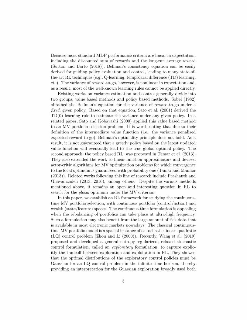
Theorem 1 The optimal value function of the entropy-regularized exploratoryMV problem (11) is given by

V (t, x;w) = (x−w)2e−ρ2(T−t)+

λρ2

4

(T 2 − t2

)−λ

2

(ρ2T − ln

σ2

πλ

)(T−t)−(w−z)2,

(23)for (t, x) ∈ [0, T ] × R. Moreover, the optimal feedback control is Gaussian,with its density function given by

π∗(u; t, x, w) = N(u∣∣∣− ρ

σ(x− w) ,

λ

2σ2eρ

2(T−t)). (24)

The associated optimal wealth process under π∗ is the unique solution of theSDE

dX∗t = −ρ2(X∗t − w) dt+

√ρ2 (X∗t − w)2 +

λ

2eρ2(T−t) dWt, X

∗0 = x0. (25)

Finally, the Lagrange multiplier w is given by w = zeρ2T−x0

eρ2T−1.

Proof. For each fixed w ∈ R, the verification arguments aim to show thatthe optimal value function of problem (11) is given by (23) and that thecandidate optimal policy (24) is indeed admissible. A detailed proof followsthe same lines of that of Theorem 4 in Wang et al. (2019), and is left forinterested readers.

We now determine the Lagrange multiplier w through the constraintE[X∗T ] = z. It follows from (25), along with the standard estimate thatE[maxt∈[0,T ](X

∗t )2]<∞ and Fubini’s Theorem, that

E[X∗t ] = x0 + E[∫ t

0−ρ2(X∗s − w) ds

]= x0 +

∫ t

0−ρ2 (E[X∗s ]− w) ds.

Hence, E[X∗t ] = (x0 −w)e−ρ2t +w. The constraint E[X∗T ] = z now becomes

(x0 − w)e−ρ2T + w = z, which gives w = zeρ

2T−x0

eρ2T−1.

12

There are several interesting points to note in this result. First of all,it follows from Theorem 2 in the next section that the classical and theexploratory MV problems have the same Lagrange multiplier value due tothe fact that the optimal terminal wealths under the respective optimalfeedback controls of the two problems turn out to have the same mean.7

This latter result is rather surprising at first sight because the explorationgreatly alters the underlying system dynamics (compare the dynamics (2)with (9)).

Second, the variance of the optimal Gaussian policy, which measures thelevel of exploration, is λ

2σ2 eρ2(T−t) at time t. So the exploration decays in

time: the agent initially engages in exploration at the maximum level, andreduces it gradually (although never to zero) as time passes and approachesthe end of the investment horizon. Hence, different from its infinite horizoncounterpart studied in Wang et al. (2019), the extent of exploration is nolonger constant, but, rather, annealing. This is intuitive because, as theRL agent learns more about the random environment as time passes, theexploitation becomes more important since there is a deadline T at which heractions will be evaluated. Naturally, exploitation dominates exploration astime approaches maturity. Theorem 1 presents such a decaying explorationscheme endogenously which, to our best knowledge, has not been derived inthe RL literature.

Third, as already noted in Wang et al. (2019), at any given t ∈ [0, T ], thevariance of the exploratory Gaussian distribution decreases as the volatilityof the risky asset increases, with other parameters being fixed. The volatilityof the risky asset reflects the level of randomness of the investment universe.This hints that a more random environment contains more learning oppor-tunities, which the RL agent can leverage to reduce her own exploratoryendeavor because, after all, exploration is costly.

Finally, the mean of the Gaussian distribution (24) is independent of theexploration weight λ, while its variance is independent of the state x. Thishighlights a perfect separation between exploitation and exploration, as theformer is captured by the mean and the latter by the variance of the optimalGaussian exploration. This property is also consistent with the LQ case inthe infinite horizon studied in Wang et al. (2019).

7Theorem 2 is a reproduction of the results on the classical MV problem obtained inZhou and Li (2000).

13

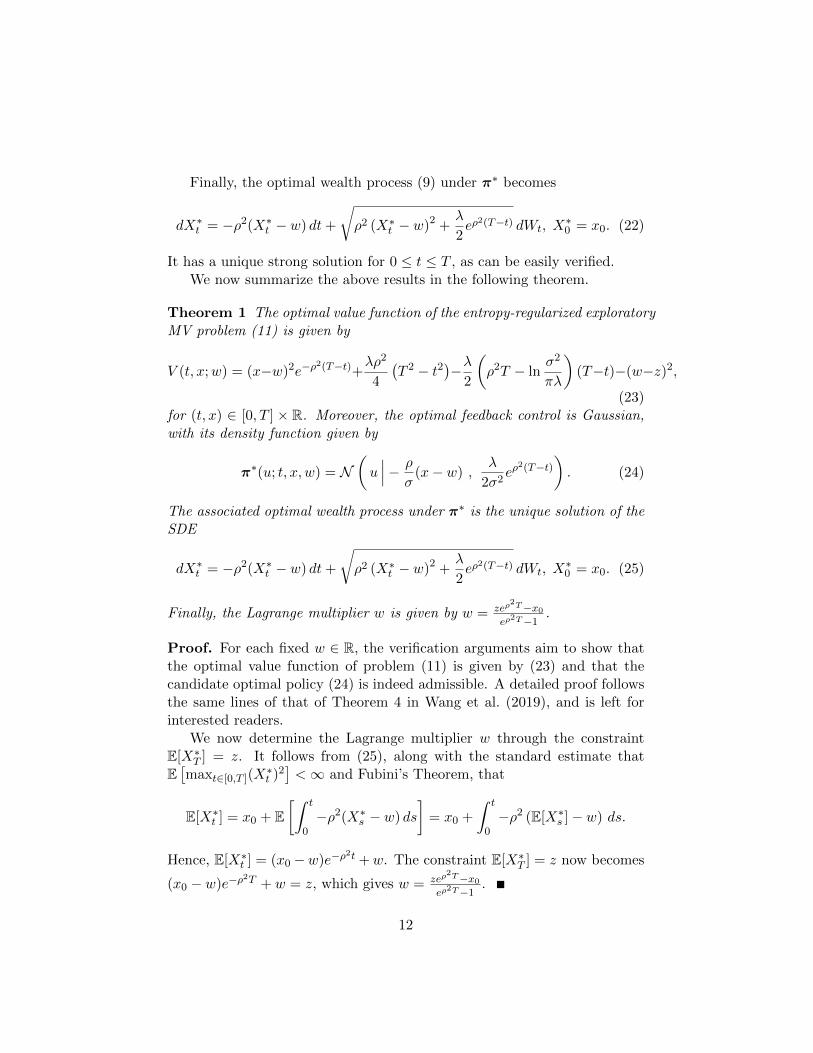
3.2 Solvability equivalence between classical and exploratoryMV problems

In this section, we establish the solvability equivalence between the classi-cal and the exploratory, entropy-regularized MV problems. Note that bothproblems can be and indeed have been solved separately and independently.Here by “solvability equivalence” we mean that the solution of one problemwill lead to that of the other directly, without needing to solve it separately.This equivalence was first discovered in Wang et al. (2019) for the infinitehorizon LQ case, and was shown to be instrumental in deriving the conver-gence result (when the exploration weight λ decays to 0) as well as analyzingthe exploration cost therein. Here, the discussions are mostly parallel; sothey will be brief.

Recall the classical MV problem (4). In order to apply dynamic pro-gramming, we again consider the set of admissible controls, Acl(s, y), for(s, y) ∈ [0, T )× R,

Acl(s, y) :=u = ut, t ∈ [s, T ]: u is Ft-progressively measurable and

E[∫ Ts (us)

2 ds] <∞.

The (optimal) value function is defined by

V cl(s, y;w) := infu∈Acl(s,y)

E[(xuT − w)2

∣∣xus = y]− (w − z)2, (26)

for (s, y) ∈ [0, T )×R, where w ∈ R is fixed. Once this problem is solved, wcan be determined by the constraint E[x∗T ] = z, with x∗t , t ∈ [0, T ] beingthe optimal wealth process under the optimal portfolio u∗.

The HJB equation is

ωt(t, x;w)+minu∈R

(1

2σ2u2ωxx(t, x;w) + ρσuωx(t, x;w)

)= 0, (t, x) ∈ [0, T )×R,

(27)with the terminal condition ω(T, x;w) = (x− w)2 − (w − z)2.

Standard verification arguments deduce the optimal value function to be

V cl(t, x;w) = (x− w)2e−ρ2(T−t) − (w − z)2,

the optimal feedback control policy to be

u∗(u; t, x, w) = −ρσ

(x− w), (28)

14

and the corresponding optimal wealth process to be the unique strong solu-tion to the SDE

dx∗t = −ρ2(x∗t − w) dt− ρ(x∗t − w) dWt, x∗0 = x0. (29)

Comparing the optimal wealth dynamics, (25) and (29), of the exploratoryand classical problems, we note that they have the same drift coefficient (butdifferent diffusion coefficients). As a result, the two problems have the samemean of optimal terminal wealth and hence the same value of the Lagrange

multiplier w = zeρ2T−x0

eρ2T−1determined by the constraint E[x∗T ] = z.

We now provide the solvability equivalence between the two problems.The proof is very similar to that of Theorem 7 in Wang et al. (2019), and isthus omitted.

Theorem 2 The following two statements (a) and (b) are equivalent.

(a) The function v(t, x;w) = (x−w)2e−ρ2(T−t)+λρ2

4

(T 2 − t2

)−λ

2

(ρ2T − ln σ2

πλ

)(T−

t) − (w − z)2, (t, x) ∈ [0, T ] × R, is the optimal value function of theexploratory MV problem (11), and the corresponding optimal feedbackcontrol is

π∗(u; t, x, w) = N(u∣∣∣− ρ

σ(x− w) ,

λ

2σ2eρ

2(T−t)).

(b) The function ω(t, x;w) = (x−w)2e−ρ2(T−t)−(w−z)2, (t, x) ∈ [0, T ]×R,

is the optimal value function of the classical MV problem (26), and thecorresponding optimal feedback control is

u∗(t, x;w) = −ρσ

(x− w).

Moreover, the two problems have the same Lagrange multiplier w = zeρ2T−x0

eρ2T−1.

It is reasonable to expect that the exploratory problem converges toits classical counterpart as the exploration weight λ decreases to 0. Thefollowing result makes this precise.

Theorem 3 Assume that statement (a) (or equivalently, (b)) of Theorem2 holds. Then, for each (t, x, w) ∈ [0, T ]× R× R,

limλ→0

π∗(·; t, x;w) = δu∗(t,x;w)(·) weakly.

Moreover,limλ→0|V (t, x;w)− V cl(t, x;w)| = 0.

15

Proof. The weak convergence of the feedback controls follows from theexplicit forms of π∗ and u∗ in statements (a) and (b). The pointwise con-vergence of the value functions follows easily from the forms of V (·) andV cl(·), together with the fact that

limλ→0

λ

2lnσ2

πλ= 0.

Finally, we conclude this section by examining the cost of the exploration.This was originally defined and derived in Wang et al. (2019) for the infinitehorizon setting. Here, the cost associated with the MV problem due to theexplicit inclusion of exploration in the objective (11) is defined by

Cu∗,π∗(0, x0;w) :=

(V (0, x0;w)− λE

[∫ T

0

∫Rπ∗t (u) lnπ∗t (u)du dt

∣∣∣∣Xπ∗0 = x0

])−V cl(0, x0;w), (30)

for x0 ∈ R, where π∗ = π∗t , t ∈ [0, T ] is the (open-loop) optimal strategy

generated by the optimal feedback law π∗ with respect to the initial condi-tion Xπ∗

0 = x0. This cost is the difference between the two optimal valuefunctions, adjusting for the additional contribution due to the entropy valueof the optimal exploratory strategy.

Making use of Theorem 2, we have the following result.

Theorem 4 Assume that statement (a) (or equivalently, (b)) of Theorem2 holds. Then, the exploration cost for the MV problem is

Cu∗,π∗(0, x0;w) =λT

2, x0 ∈ R, w ∈ R. (31)

Proof. Let π∗t , t ∈ [0, T ] be the open-loop control generated by the feed-back control π∗ given in statement (a) with respect to the initial state x0

at t = 0, namely,

π∗t (u) = N(u∣∣∣− ρ

σ(X∗t − w) ,

λ

2σ2eρ

2(T−t))

where X∗t , t ∈ [0, T ] is the corresponding optimal wealth process of theexploratory MV problem, starting from the state x0 at t = 0, when π∗ isapplied. Then, we easily deduce that∫

Rπ∗t (u) lnπ∗t (u)du = −1

2ln

(πeλ

σ2eρ

2(T−t)).

16

The desired result now follows immediately from the expressions of V (·) in(a) and V cl(·) in (b).

The exploration cost depends only on two “agent-specific” parameters,the exploration weight λ > 0 and the investment horizon T > 0. Notethat the latter is also the exploration horizon. Our result is intuitive inthat the exploration cost increases with the exploration weight and with theexploration horizon. Indeed, the dependence is linear with respect to eachof the two attributes: λ and T .8 It is also interesting to note that the cost isindependent of the Lagrange multiplier. This suggests that the explorationcost will not increase when the agent is more aggressive (or risk-seeking) –reflected by the expected target z or equivalently the Lagrange multiplierw.

4 RL Algorithm Design

Having laid the theoretical foundation in the previous two sections, we nowdesign an RL algorithm to learn the solution of the entropy-regularized MVproblem and to output implementable portfolio allocation strategies, with-out assuming any knowledge about the underlying parameters. To thisend, we will first establish a so-called policy improvement theorem as wellas the corresponding convergence result. Meanwhile, we will provide a self-correcting scheme to learn the true Lagrange multiplier w, based on stochas-tic approximation. Our RL algorithm bypasses the phase of estimatingany model parameters, including the mean return vector and the variance-covariance matrix. It also avoids inverting a typically ill-conditioned variance-covariance matrix in high dimensions that would likely produce non-robustportfolio strategies.

In this paper, rather than relying on the typical framework of discrete-time MDP (that is used for most RL problems) and discretizing time andspace accordingly, we design an algorithm to learn the solutions of thecontinuous-time exploratory MV problem (11) directly. Specifically, weadopt the approach developed in Doya (2000) to avoid discretization of thestate dynamics or the HJB equation. As pointed out in Doya (2000), itis typically challenging to find the right granularity to discretize the state,action and time, and naive discretization may lead to poor performance. On

8In Wang et al. (2019) with the infinite horizon LQ case, an analogous result is obtainedwhich states that exploration cost is proportional to the exploration weight and inverselyproportional to the discount factor. Clearly, here the length of time horizon, T , plays arole similar to the inverse of the discount factor.

17

the other hand, grid-based discretization methods for solving the HJB equa-tion cannot be easily extended to high-dimensional state space in practicedue to the curse of dimensionality, although theoretical convergence resultshave been established (see Munos and Bourgine (1998); Munos (2000)). Ouralgorithm, to be described in Subsection 4.2, however, makes use of a prov-able policy improvement theorem and fairly simple yet efficient functionalapproximations to directly learn the value functions and the optimal Gaus-sian policy. Moreover, it is computationally feasible and implementable inhigh-dimensional state spaces (i.e., in the case of a large number of riskyassets) due to the explicit representation of the value functions and theportfolio strategies, thereby devoid of the curse of dimensionality. Notethat our algorithm does not use (deep) neural networks, which have beenapplied extensively in literature for (high-dimensional) continuous RL prob-lems (e.g., Lillicrap et al. (2016), Mnih et al. (2015)) but known for unstableperformance, sample inefficiency as well as extensive hyperparameter tuning(Mnih et al. (2015)), in addition to their low interpretability.9

4.1 A policy improvement theorem

Most RL algorithms consist of two iterative procedures: policy evaluationand policy improvement (Sutton and Barto (2018)). The former provides anestimated value function for the current policy, whereas the latter updatesthe current policy in the right direction to improve the value function. Apolicy improvement theorem (PIT) is therefore a crucial prerequisite forinterpretable RL algorithms that ensures the iterated value functions tobe non-increasing (in the case of a minimization problem), and ultimatelyconverge to the optimal value function; see, for example, Section 4.2 ofSutton and Barto (2018). PITs have been proved for discrete-time entropy-regularized RL problems in infinite horizon (Haarnoja et al. (2017)), and forcontinuous-time classical stochastic control problems (Jacka and Mijatovic(2017)).10 The following result provides a PIT for our exploratory MVportfolio selection problem.

Theorem 5 (Policy Improvement Theorem) Let w ∈ R be fixed andπ = π(·; ·, ·, w) be an arbitrarily given admissible feedback control policy.

9Interpretability is one of the most important and pressing issues in the general arti-ficial intelligence applications in financial industry due to, among others, the regulatoryrequirement.

10Jacka and Mijatovic (2017) studied classical stochastic control problems with nodistributional controls nor entropy regularization. They did not consider RL and relatedissues including exploration.

18

Suppose that the corresponding value function V π(·, ·;w) ∈ C1,2([0, T ) ×R)∩C0([0, T ]×R) and satisfies V πxx(t, x;w) > 0, for any (t, x) ∈ [0, T )×R.Suppose further that the feedback policy π defined by

π(u; t, x, w) = N(u∣∣∣− ρ

σ

V πx (t, x;w)

V πxx(t, x;w),

λ

σ2V πxx(t, x;w)

)(32)

is admissible. Then,

V π(t, x;w) ≤ V π(t, x;w), (t, x) ∈ [0, T ]× R. (33)

Proof. Fix (t, x) ∈ [0, T ]×R. Since, by assumption, the feedback policy πis admissible, the open-loop control strategy, π = πv, v ∈ [t, T ], generatedfrom π with respect to the initial condition Xπ

t = x is admissible. LetXπ

s , s ∈ [t, T ] be the corresponding wealth process under π. ApplyingIto’s formula, we have

V π(s, Xs) = V π(t, x) +

∫ s

tV πt (v,Xπ

v )dv +

∫ s

t

∫R

(1

2σ2u2V πxx(v,Xπ

v )

+ρσuV πx (v,Xπv ))πv(u) dudv+

∫ s

tσ

(∫Ru2πv(u)du

) 12

V π(v,Xπv ) dWv, s ∈ [t, T ].

(34)

Define the stopping times τn := infs ≥ t :∫ st σ

2∫R u

2πv(u)du(V π(v,Xπ

v ))2dv ≥

n, for n ≥ 1. Then, from (34), we obtain

V π(t, x) = E[V π(s ∧ τn, Xπ

s∧τn)−∫ s∧τn

tV πt (v,Xπ

v )dv

−∫ s∧τn

t

∫R

(1

2σ2u2V πxx(v,Xπ

v ) + ρσuV πx (v,Xπv ))πv(u) dudv

∣∣∣Xπt = x

].

(35)On the other hand, by standard arguments and the assumption that V π issmooth, we have

V πt (t, x)+

∫R

(1

2σ2u2V πxx(t, x) + ρσuV πx (t, x) + λ lnπ(u; t, x)

)π(u; t, x)du = 0,

for any (t, x) ∈ [0, T )× R. It follows that

V πt (t, x)+ minπ′∈P(R)

∫R

(1

2σ2u2V πxx(t, x) + ρσuV πx (t, x) + λ lnπ′(u)

)π′(u)du ≤ 0.

(36)

19

Notice that the minimizer of the Hamiltonian in (36) is given by the feedbackpolicy π in (32). It then follows that equation (35) implies

V π(t, x) ≥ E[V π(s ∧ τn, Xπ

s∧τn) + λ

∫ s∧τn

t

∫Rπv(u) ln πv(u) dudv

∣∣∣Xπt = x

],

for (t, x) ∈ [0, T ] × R and s ∈ [t, T ]. Now taking s = T , and using thatV π(T, x) = V π(T, x) = (x−w)2−(w−z)2 together with the assumption thatπ is admissible, we obtain, by sending n→∞ and applying the dominatedconvergence theorem, that

V π(t, x) ≥ E[V π(T,Xπ

T )+λ

∫ T

t

∫Rπv(u) ln πv(u) dudv

∣∣∣Xπt = x

]= V π(t, x),

for any (t, x) ∈ [0, T ]× R.

The above theorem suggests that there are always policies in the Gaus-sian family that improves the value function of any given, not necessarilyGaussian, policy. Hence, without loss of generality, we can simply focuson the Gaussian policies when choosing an initial solution. Moreover, theoptimal Gaussian policy (24) in Theorem 1 suggests that a candidate initialfeedback policy may take the form π0(u; t, x, w) = N (u|a(x−w), c1e

c2(T−t)).It turns out that, theoretically, such a choice leads to the convergence of boththe value functions and the policies in a finite number of iterations.

Theorem 6 Let π0(u; t, x, w) = N (u|a(x − w), c1ec2(T−t)), with a, c2 ∈ R

and c1 > 0. Denote by πn(u; t, x, w), (t, x) ∈ [0, T ]×R, n ≥ 1 the sequenceof feedback policies updated by the policy improvement scheme (32), andV πn(t, x;w), (t, x) ∈ [0, T ] × R, n ≥ 1 the sequence of the correspondingvalue functions. Then,

limn→∞

πn(·; t, x, w) = π∗(·; t, x, w) weakly, (37)

andlimn→∞

V πn(t, x;w) = V (t, x;w), (38)

for any (t, x, w) ∈ [0, T ]×R×R, where π∗ and V are the optimal Gaussianpolicy (24) and the optimal value function (23), respectively.

Proof. It can be easily verified that the feedback policy π0 where π0(u; t, x, w) =N (u|a(x−w), c1e

c2(T−t)) generates an open-loop policy π0 that is admissible

20

with respect to the initial (t, x). Moreover, it follows from the Feynman-Kacformula that the corresponding value function V π0 satisfies the PDE

V π0t (t, x;w) +

∫R

(1

2σ2u2V π0

xx (t, x;w) + ρσuV π0x (t, x;w)

+λ lnπ0(u; t, x, w))π0(u; t, x, w)du = 0, (39)

with terminal condition V π0(T, x;w) = (x − w)2 − (w − z)2. Solving thisequation we obtain

V π0(t, x;w) = (x− w)2e(2ρσa+σ2a2)(T−t) +

∫ T

tc1σ

2e(2ρσa+σ2a2+c2)(T−s)ds

+λc2

4(T − t)2 +

λ ln(2πec1)

2(T − t)− (w − z)2. (40)

It is easy to check that V π0 satisfies the conditions in Theorem 5 and, hence,the theorem applies. The improved policy is given by (32), which, in thecurrent case, becomes

π1(u; t, x, w) = N(u∣∣∣− ρ

σ(x− w) ,

λ

2σ2e(2ρσa+σ2a2)(T−t)

).

Again, we can calculate the corresponding value function as V π1(t, x;w) =(x − w)2e−ρ

2(T−t) + F1(t), where F1 is a function of t only. Theorem 5 isapplicable again, which yields the improved policy π2 as exactly the optimalGaussian policy π∗ given in (24), together with the optimal value functionV in (23). The desired convergence therefore follows, as for n ≥ 2, boththe policy and the value function will no longer strictly improve under thepolicy improvement scheme (32).

The above convergence result shows that if we choose the initial policywisely, the learning scheme will, theoretically, converge after a finite num-ber of (two, in fact) iterations. When implementing this scheme in prac-tice, of course, the value function for each policy can only be approximatedand, hence, the learning process typically takes more iterations to converge.Nevertheless, Theorem 5 provides the theoretical foundation for updating acurrent policy, while Theorem 6 suggests a good starting point in the policyspace. We will make use of both results in the next subsection to design animplementable RL algorithm for the exploratory MV problem.

21

4.2 The EMV algorithm

In this section, we present an RL algorithm, the EMV (exploratory mean–variance) algorithm, to solve (11). It consists of three concurrently ongo-ing procedures: the policy evaluation, the policy improvement and a self-correcting scheme for learning the Lagrange multiplier w based on stochasticapproximation.

For the policy evaluation, we follow the method employed in Doya (2000)for learning the value function V π under any arbitrarily given admissiblefeedback policy π. By Bellman’s consistency, we have

V π(t, x) = E[V π(s,Xs) + λ

∫ s

t

∫Rπv(u) lnπv(u)dudv

∣∣Xt = x

], s ∈ [t, T ],

(41)for (t, x) ∈ [0, T ]×R. Rearranging this equation and dividing both sides bys− t, we obtain

E[V π(s,Xs)− V π(t,Xt)

s− t+

λ

s− t

∫ s

t

∫Rπv(u) lnπv(u)dudv

∣∣Xt = x

]= 0.

Taking s→ t gives rise to the continuous-time Bellman’s error (or the tem-proral difference (TD) error; see Doya (2000))

δt := V πt + λ

∫Rπt(u) lnπt(u)du, (42)

where V πt =V π(t+∆t,Xt+∆t)−V π(t,Xt)

∆t is the total derivative and ∆t is thediscretization step for the learning algorithm.

The objective of the policy evaluation procedure is to minimize the Bell-man’s error δt. In general, this can be carried out as follows. Denote by V θ

and πφ respectively the parametrized value function and policy (upon usingregressions or neural networks, or making use of some of the structures ofthe problem; see below), with θ, φ being the vector of weights to be learned.We then minimize

C(θ, φ) =1

2E[∫ T

0|δt|2dt

]=

1

2E[∫ T

0

∣∣V θt + λ

∫Rπφt (u) lnπφt (u)du

∣∣2dt] ,where πφ = πφt , t ∈ [0, T ] is generated from πφ with respect to a giveninitial state X0 = x0 at time 0. To approximate C(θ, φ) in an implementablealgorithm, we first discretize [0, T ] into small equal-length intervals [ti, ti+1],i = 0, 1, · · · , l, where t0 = 0 and tl+1 = T . Then we collect a set of samples

22

D = (ti, xi), i = 0, 1, · · · , l + 1 in the following way. The initial sample is

(0, x0) for i = 0. Now, at each ti, i = 0, 1, · · · , l, we sample πφti to obtain anallocation ui ∈ R in the risky asset, and then observe the wealth xi+1 at thenext time instant ti+1. We can now approximate C(θ, φ) by

C(θ, φ) =1

2

∑(ti,xi)∈D

(V θ(ti, xi) + λ

∫Rπφti(u) lnπφti(u)du

)2

∆t. (43)

Instead of following the common practice to represent V θ, πφ using(deep) neural networks for continuous RL problems, in this paper we willtake advantage of the more explicit parametric expressions obtained in The-orem 1 and Theorem 6. This will lead to faster learning and convergence,which will be demonstrated in all the numerical experiments below. Moreprecisely, by virtue of Theorem 6, we will focus on Gaussian policies withvariance taking the form c1e

c2(T−t), which in turn leads to the entropyparametrized by H(πφt ) = φ1 + φ2(T − t), where φ = (φ1, φ2)′, with φ1 ∈ Rand φ2 > 0, is the parameter vector to be learned.

On the other hand, as suggested by the theoretical optimal value func-tion (23) in Theorem 1, we consider the parameterized V θ, where θ =(θ0, θ1, θ2, θ3)′, by

V θ(t, x) = (x− w)2e−θ3(T−t) + θ2t2 + θ1t+ θ0, (t, x) ∈ [0, T ]× R. (44)

From the policy improvement updating scheme (32), it follows that the

variance of the policy πφt is λ2σ2 e

θ3(T−t), resulting in the entropy 12 ln πeλ

σ2 +θ32 (T − t). Equating this with the previously derived form H(πφt ) = φ1 +φ2(T − t), we deduce

σ2 = λπe1−2φ1 and θ3 = 2φ2 = ρ2. (45)

The improved policy, in turn, becomes, according to (32), that

π(u; t, x, w) = N(u∣∣∣− ρ

σ(x− w) ,

λ

2σ2eθ3(T−t)

)

= N

(u∣∣∣−√2φ2

λπe

2φ1−12 (x− w) ,

1

2πe2φ2(T−t)+2φ1−1

), (46)

where we have assumed that the true (unknown) Sharpe ratio ρ > 0.

Rewriting the objective (43) using H(πφt ) = φ1 + φ2(T − t), we obtain

C(θ, φ) =1

2

∑(ti,xi)∈D

(V θ(ti, xi)− λ(φ1 + φ2(T − t))

)2∆t.

23

Note that V θ(ti, xi) = V θ(ti+1,xi+1)−V θ(ti,xi)∆t , with θ3 = 2φ2 in the parametriza-

tion of V θ(ti, xi). It is now straightforward to devise the updating rules for(θ1, θ2)′ and (φ1, φ2)′ using stochastic gradient descent algorithms (see, forexample, Chapter 8 of Goodfellow et al. (2016)). Precisely, we compute

∂C

∂θ1=

∑(ti,xi)∈D

(V θ(ti, xi)− λ(φ1 + φ2(T − ti))

)∆t; (47)

∂C

∂θ2=

∑(ti,xi)∈D

(V θ(ti, xi)− λ(φ1 + φ2(T − ti))

)(t2i+1 − t2i ); (48)

∂C

∂φ1= −λ

∑(ti,xi)∈D

(V θ(ti, xi)− λ(φ1 + φ2(T − ti))

)∆t; (49)

∂C

∂φ2=

∑(ti,xi)∈D

(V θ(ti, xi)− λ(φ1 + φ2(T − ti))

)∆t

×

(−2(xi+1 − w)2e−2φ2(T−ti+1)(T − ti+1)− 2(xi − w)2e−2φ2(T−ti)(T − ti)

∆t− λ(T − ti)

).

(50)Moreover, the parameter θ3 is updated with θ3 = 2φ2, and θ0 is updatedbased on the terminal condition V θ(T, x;w) = (x − w)2 − (w − z)2, whichyields

θ0 = −θ2T2 − θ1T − (w − z)2. (51)

Finally, we provide a scheme for learning the underlying Lagrange mul-tiplier w. Indeed, the constraint E[XT ] = z itself suggests the standardstochastic approximation update

wn+1 = wn − αn(XT − z), (52)

with αn > 0, n ≥ 1, being the learning rate. In implementation, we canreplace XT in (52) by a sample average 1

N

∑j x

jT to have a more stable

learning process (see, for example, Section 1.1 of Kushner and Yin (2003)),where N ≥ 1 is the sample size and xjT ’s are the most recent N terminalwealth values obtained at the time when w is to be updated. It is interestingto notice that the learning scheme of w, (52), is statistically self-correcting.For example, if the (sample average) terminal wealth is above the target z,the updating rule (52) will decrease w, which in turn decreases the meanof the exploratory Gaussian policy π in view of (46). This implies that

24

there will be less risky allocation in the next step of actions for learning andoptimizing, leading to, on average, a decreased terminal wealth.11

We now summarize the pseudocode for the EMV algorithm.

Algorithm 1 EMV: Exploratory Mean-Variance Portfolio Selection

Input: Market Simulator Market, learning rates α, ηθ, ηφ, initial wealthx0, target payoff z, investment horizon T , discretization ∆t, explorationrate λ, number of iterations M , sample average size N .Initialize θ, φ and wfor k = 1 to M dofor i = 1 to b T∆tc do

Sample (tki , xki ) from Market under πφ

Obtain collected samples D = (tki , xki ), 1 ≤ i ≤ b T∆tcUpdate θ ← θ − ηθ∇θC(θ, φ) using (47) and (48)Update θ0 using (51) and θ3 ← 2φ2

Update φ← φ− ηφ∇φC(θ, φ) using (49) and (50)end for

Update πφ ← N(u∣∣∣−√2φ2

λπ e2φ1−1

2 (x− w) , 12πe

2φ2(T−t)+2φ1−1

)if k mod N == 0

Update w ← w − α(

1N

∑kj=k−N+1 x

j

b T∆tc − z

)end if

end for

5 Simulation Results

In this section, we compare the performance of our RL algorithm EMV withtwo other methods that could be used to solve the classical MV problem(3). The first one is the traditional maximum likelihood estimation (MLE)that relies on the real-time estimation of the drift µ and the volatility σin the geometric Brownian motion price model (1). Once the estimators ofµ and σ are available using the most recent price time series, the portfolioallocation can be computed using the optimal allocation (28) for the classicalMV problem. Another alternative is based on the deep deterministic policygradient (DDPG) method developed by Lillicrap et al. (2016), a method

11This discussion here is based on the assumption that the market has a positive Sharperatio (recall (46)). The case of a negative Sharpe ratio can be dealt with similarly.

25

that has been taken as the baseline approach for comparisons of differentRL algorithms that solve continuous control problems.

We conduct comparisons in various simulation settings, including thestationary setting where the price of the risky asset evolves according to thegeometric Brownian motion (1) and the non-stationary setting that involvesstochastic factor modeling for the drift and volatility parameters. We alsoconsider a time-decreasing exploration case which can be easily accommo-dated by the EMV through an annealing λ across all the episodes [0, T ] inthe learning process. In nearly all of the experiments, our EMV algorithmoutperforms the other two methods by large margins.

In the following, we briefly describe the two other methods.

Maximum likelihood estimation (MLE)The MLE is a popular method for estimating the parameters µ and σ inthe geometric Brownian motion model (1). We refer the interested readersto Section 9.3.2 of Campbell et al. (1997) for a detailed description of thismethod. At each decision making time ti, the MLE estimators for µ and σare calculated based on the most recent 100 data points of the price. Onecan then substitute the MLE estimators into the optimal allocation (28)

and the expression of the Lagrange multiplier w = zeρ2T−x0

eρ2T−1to compute

the allocation ui ∈ R in the risky asset. Such a two-phase procedure iscommonly used in adaptive control, where the first phase is identificationand the second one is optimization (see, for example, Chen and Guo (2012),Kumar and Varaiya (2015)). The real-time estimation procedure also allowsthe MLE to be applicable in non-stationary markets with time-varying µ andσ.

Deep deterministic policy gradient (DDPG)The DDPG method has attracted significant attention since it was intro-duced in Lillicrap et al. (2016). It has been taken as a state-of-the-artbaseline approach for continuous control (action) RL problems, albeit indiscrete time. The DDPG learns a deterministic target policy using deepneural networks for both the critic and the actor, with exogenous noise beingadded to encourage exploration (e.g. using OU processes; see Lillicrap et al.(2016) for details). To adapt the DDPG to the classical MV setting (with-out entropy regularization), we make the following adjustments. Since thetarget policy we aim to learn is a deterministic function of (x−w) (see (28)),we will feed the samples xi−w, rather than only xi, to the actor network inorder to output the allocation ui ∈ R. Here, w is the learned Lagrange mul-tiplier at the decision making time ti, obtained from the same self-correcting

26

scheme (52). This modification also enables us to connect current allocationwith the previously obtained sample average of terminal wealth in a feed-back loop, through the Lagrange multiplier w. Another modification fromthe original DDPG is that we include prioritized experience replay (Schaulet al. (2016)), rather than sampling experience uniformly from the replaybuffer. We select the terminal experience with higher probability to trainthe critic and actor networks, to account for the fact that the MV problemhas no running cost, but only a terminal cost given by (xT −w)2 − (w − z)(cf. (4)). Such a modification significantly improves learning speed andperformance.

5.1 The stationary market case

We first perform numerical simulations in a stationary market environment,where the price process is simulated according to the geometric Brownianmotion (1) with constant µ and σ. We take T = 1 and ∆t = 1

252 , indicat-ing that the MV problem is considered over a one-year period, with dailyrebalancing. Reasonable values of the annualized return and volatility willbe taken from the sets µ ∈ −50%,−30%,−10%, 0%, 10%, 30%, 50% andσ ∈ 10%, 20%, 30%, 40%, respectively. These values are usually consideredfor a “typical” stock for simulation purpose (see, for example, Hutchinsonet al. (1994)). The annualized interest rate is taken to be r = 2%. Weconsider the MV problem with a 40% annualized target return on the ter-minal wealth starting from a normalized initial wealth x0 = 1 and, hence,z = 1.4 in (3). These model parameters will be fixed for all the simulationsconsidered in this paper.

For the EMV algorithm, we take the total training episodes M = 20000and the sample size N = 10 for learning the Lagrange multiplier w. Thetemperature parameter λ = 2. Across all the simulations in this section, thelearning rates are fixed as α = 0.05 and ηθ = ηφ = 0.0005.

We choose the same M and N for the DDPG algorithm for a fair com-parison. The critic network has 3 hidden layers with 10, 8, 8 hidden unitsfor each layer, and the actor network has 2 hidden layers with 10, 8 hiddenunits. The learning rates for the critic and actor are 0.0001, fixed acrossall simulations in this section as the case for EMV. The replay buffer hassize 80, and the minibatch size is 20 for the stochastic gradient decent. Thetarget network has the soft update parameter τ = 0.001. Finally, we adoptthe OU process for adding exploration noise; see Lillicrap et al. (2016) formore details. All the simulations using the DDPG algorithm were trainedin Tensorflow.

27

We summarize in Table 1 the simulation results for the three methods,EMV, MLE and DDPG, under market scenarios corresponding to differentcombinations of µ’s and σ’s. For each method under each market scenario,we present the annualized sample mean M and sample variance V of thelast 2000 terminal wealth, and the corresponding annualized Sharpe ratio

SR = M−1√V

.

A few observations are in order. First of all, the EMV algorithm outper-forms the other two methods by a large margin in several statistics of theinvestment outcome including sample mean, sample variance and Sharperatio. In fact, based on the comparison of Sharpe ratios, EMV outper-forms MLE in all the 28 experiments, and outperforms DDPG in 23 out ofthe total 28 experiments. Notice that DDPG yields rather unstable perfor-mance across different market scenarios, with some of the sample averageterminal wealth below 0 indicating the occurrence of bankruptcy. The EMValgorithm, on the other hand, achieves positive annualized return in all theexperiments. The advantage of the EMV algorithm over the deep learningDDPG algorithm is even more significant if we take into account the train-ing time (all the experiments were performed on a MacBook Air laptop).Indeed, DDPG involves extensive training of two deep neural networks, mak-ing it less appealing for high-frequency portfolio rebalancing and trading inpractice.

Another advantage of EMV over DDPG is the ease of hyperparametertuning. Recall that the learning rates are fixed respectively for EMV andDDPG across all the experiments for different µ’s and σ’s. The perfor-mance of the EMV algorithm is less affected by the fixed learning rates,while the DDPG algorithm is not. Indeed, DDPG has been noted for itsnotorious brittleness and hyperparameter sensitivity in practice (see, for ex-ample, Duan et al. (2016), Henderson et al. (2018)), issues also shared byother deep RL methods for continuous control problems. Our EMV algo-rithm does not suffer from such issues, as a result of avoiding deep neuralnetworks in its training and decision making processes.

The MLE method, although free from any learning rates tuning, needs toestimate the underlying parameters µ and σ. In all the simulations presentedin Table 1, the estimated value of σ is relatively close to its true value, whilethe drift parameter µ cannot be estimated accurately. This is consistentwith the well documented mean–blur problem, which in turn leads to highervariance of the terminal wealth (see Table 1) when one applies the estimatedµ and σ to select the risky allocation (28).

Finally, we present the learning curves for the three methods in Figure 1

28

Table 1: Comparison of the annualized sample mean (M),sample variance (V ), Sharpe ratio (SR) and average trainingtime (per experiment) for EMV, MLE and DDPG.14

Market scenarios EMV MLE DDPG

µ = −50%, σ = 10% 1.396; 0.006; 5.107 1.556; 0.017; 4.284 1.297; 0.107; 0.908µ = −30%, σ = 10% 1.390; 0.016; 3.039 1.215; 0.014; 1.833 1.401; 0.003; 7.076µ = −10%, σ = 10% 1.330; 0.074; 1.218 1.056; 1.365; 0.482 0.901; 0.014; -0.833µ = 0%, σ = 10% 1.204; 1.280; 0.180 0.926; 38.40; -0.012 1.029; 0.038; 0.147µ = 10%, σ = 10% 1.318; 0.171; 0.769 1.009; 0.453; 0.014 0.951; 0.008; -0.541µ = 30%, σ = 10% 1.385; 0.019; 2.785 1.179; 0.059; 0.737 0.224; 0.104; -2.405µ = 50%, σ = 10% 1.394; 0.007; 4.772 1.459; 0.013; 3.983 1.478; 0.667; 0.717µ = −50%, σ = 20% 1.387; 0.022; 2.606 1.310; 0.050; 1.387 -0.551; 0.425; -2.379µ = −30%, σ = 20% 1.359; 0.051; 1.598 1.205; 1.319; 0.178 1.973; 0.404; 1.531µ = −10%, σ = 20% 1.309; 0.245; 0.625 1.036; 2.183; 0.024 1.349; 0.368; 0.575µ = 0%, σ = 20% 1.105; 0.727; 0.123 0.921; 6.887; -0.301 0.988; 0.139; -0.033µ = 10%, σ = 20% 1.221; 0.314; 0.395 1.045; 6.751; 0.017 1.243; 0.354; 0.408µ = 30%, σ = 20% 1.345; 0.062; 1.387 1.155; 1.743; 0.117 1.360; 0.050; 1.613µ = 50%, σ = 20% 1.385; 0.027; 2.350 1.237; 1.293; 0.208 1.385; 0.004; 6.496µ = −50%, σ = 30% 1.353; 0.044; 1.682 1.333; 9.465; 0.108 0.272; 2.762; -0.438µ = −30%, σ = 30% 1.323; 0.106; 0.992 1.092; 5.657; 0.039 0.034; 0.924; -1.005µ = −10%, σ = 30% 1.317; 0.696; 0.380 1.045; 17.87; 0.011 1.371; 0.792; 0.417µ = 0%, σ = 30% 1.079; 0.727; 0.092 0.955; 28.84; -0.008 1.070; 0.752; 0.081µ = 10%, σ = 30% 1.282; 0.885; 0.300 0.885; 24.06; -0.023 1.243; 0.825; 0.268µ = 30%, σ = 30% 1.334; 0.131; 0.921 0.886; 24.41; -0.023 1.210; 0.921; 0.218µ = 50%, σ = 30% 1.350; 0.049; 1.583 1.238; 7.505; 0.087 0.610; 0.143 -1.030µ = −50%, σ = 40% 1.342; 0.061; 1.385 1.284; 11.14; 0.085 1.328; 0.501; 0.463µ = −30%, σ = 40% 1.320; 0.146; 0.839 1.145; 3.315; 0.080 1.212; 0.160; 0.531µ = −10%, σ = 40% 1.241; 0.707; 0.287 0.979; 7.960; -0.007 1.335; 1.413; 0.282µ = 0%, σ = 40% 1.057; 0.671; 0.070 0.950; 31.60; -0.009 1.064; 1.467; 0.053µ = 10%, σ = 40% 1.155; 0.591; 0.202 1.053; 9.090; 0.017 1.242; 1.499; 0.198µ = 30%, σ = 40% 1.320; 0.198; 0.716 1.083; 17.46; 0.020 0.179; 1.533; -0.663µ = 50%, σ = 40% 1.329; 0.078; 1.174 0.963; 43.17; -0.006 -0.390; 1.577; -1.107

Training time < 10s < 10s ≈ 3hrs

14If the hyperparameters are allowed to be tuned on a scenario-by-scenario basis (i.e.,not for comparison purpose), the performance of EMV can be further improved with theShape ratio close to its theoretical maximum, whereas improvement is more difficult toachieve for DDPG by hyperparameter tuning.

29

and Figure 2. We plot the changes of the sample mean and sample varianceof every (non-overlapping) 50 terminal wealth, as the learning proceeds foreach method.12 From these plots, we can see that the EMV algorithmconverges relatively faster than the other two methods, achieving relativelygood performance even in the early phase of the learning process. This isalso consistent with the convergence result in Theorem 6 and the remarksimmediately following it in Section 4.1.

0 50 100 150 200 250 300 350 400Aggregated episodes (50)

-0.5

0

0.5

1

1.5

2

2.5

3

3.5

Sam

ple

mea

n

DDPGMLEEMVTarget z=1.4

Figure 1: Learning curves of sample means of terminal wealth (over every50 iterations) for EMV, MLE and DDPG (µ = −30%, σ = 10%).

12Note the log scale for the variance in Figure 2.

30

0 50 100 150 200 250 300 350 400Aggregated episodes (50)

10-4

10-3

10-2

10-1

100

101

102

103

Sam

ple

varia

nce

DDPGMLEEMV

Figure 2: Learning curves of sample variances of terminal wealth (over every50 iterations) for EMV, MLE and DDPG (µ = −30%, σ = 10%).

5.2 The non-stationary market case

When it comes to the application domains of RL, one of the major differ-ences between quantitative finance and other domains (such as AlphaGo; seeSilver et al. (2016)) is that the underlying unknown investment environmentis typically time-varying with the former. In this subsection, we consider theperformance of the previous three methods in the non-stationary scenariowhere the price process is modeled by a stochastic factor model. To havea well-defined learning problem, the stochastic factor needs to change at amuch slower time-scale, compared to that of the learning process. Specifi-cally, we take the slow factor model within a multi-scale stochastic volatilitymodel framework (see, for example, Fouque et al. (2003)). The price processfollows

dSt = St(µt dt+ σ dWt), 0 < t ≤ T, S0 = s0 > 0,

with µt, σt, t ∈ [0, T ], being respectively the drift and volatility processesrestricted to each simulation episode [0, T ] (so they may vary across differ-ent episodes). The controlled wealth dynamics over each episode [0, T ] istherefore

dxut = σtut(ρt dt+ dWt), 0 < t ≤ T, xu0 = x0 ∈ R. (53)

31

For simulations in this subsection, we take

dρt = δdt and dσt = σt(δ dt+√δ dW 1

t ), 0 < t ≤MT, (54)

with ρ0 ∈ R and σ0 > 0 being the initial values respectively, δ > 0 being asmall parameter, and the two Brownian motions satisfying d〈W,W 1〉t = γdt,with |γ| < 1. Notice that the terminal horizon for the stochastic factormodel (54) is MT (recall M = 20000 and T = 1 as in Subsection 5.1),indicating that the stochastic factors ρt and σt change across all the Mepisodes. To make sure that their values stay in reasonable ranges afterrunning for all M episodes, we take δ to be small with value δ = 0.0001,and ρ0 = −3.2, σ0 = 10%, corresponding to the case µ0 = −30% initially.We plot the learning curves in Figure 3 and Figure 4. Clearly, the EMValgorithm displays remarkable stability for learning performance, comparedto the other two methods even in the non-stationary market scenario.

0 50 100 150 200 250 300 350 400Aggregated episodes (50)

-4

-2

0

2

4

6

8

10

Sam

ple

mea

n

DDPGMLEEMVTarget z=1.4

Figure 3: Learning curves of sample means of terminal wealth (over every 50iterations) for EMV, MLE and DDPG for non-stationary market scenario(µ0 = −30%, σ0 = 10%, δ = 0.0001, γ = 0).

32

0 50 100 150 200 250 300 350 400Aggregated episodes (50)

10-6

10-4

10-2

100

102

104

Sam

ple

varia

nce

DDPGMLEEMV

Figure 4: Learning curves of sample variances of terminal wealth (over every50 iterations) for EMV, MLE and DDPG for non-stationary market scenario(µ0 = −30%, σ0 = 10%, δ = 0.0001, γ = 0).

5.3 The decaying exploration case

A decaying exploration scheme is often desirable for RL since exploitationought to gradually take more weight over exploration, as more learning it-erations have been carried out.15 Within the current entropy-regularizedrelaxed stochastic control framework, we have been able to show the conver-gence from the solution of the exploratory MV to that of the classical MVin Theorem 3, as the tradeoff parameter λ→ 0. Putting together Theorem3 and Theorem 6, we can reasonably expect a further improvement of theEMV algorithm when it adopts a decaying λ scheme, rather than a constantλ as in the previous two sections. Our numerical simulation result reportedin Figure 5 demonstrates slightly improved performance of the EMV algo-rithm with a specifically chosen λ process that decreases across all the Mepisodes, given by

λk = λ0

(1− exp

(200(k −M)

M

)), for k = 0, 1, 2, . . . ,M. (55)

15It is important to distinguish between decaying during a given learning episode [0, T ]and decaying during the entire learning process (across different episodes). The formerhas been derived in Theorem 1 as the decay of the Gaussian variance in t. The latterrefers to the notion that less exploration is needed in later learning episodes.

33

We plot the histogram of the last 2000 values of terminal wealth generatedby the EMV algorithm with the decaying λ scheme starting from λ0 = 2 andthe original EMV algorithm with constant λ = 2, respectively. The Sharperatio increases from 3.039 to 3.243. The result in Figure 5 corresponds tothe stationary market case; the case for non-stationary market demonstratessimilar improvement by adopting the decaying exploration scheme.

Figure 5: Histogram of the last 2000 values of terminal wealth for EMVwith constant λ and decaying λ (µ = −30%, σ = 10%).

6 Conclusions

In this paper we have developed an RL framework for the continuous-timeMV portfolio selection, using the exploratory stochastic control formulationrecently proposed and studied in Wang et al. (2019). By recasting the MVportfolio selection as an exploration/learning and exploitation/optimizationproblem, we are able to derive a data-driven solution, completely skippingany estimation of the unknown model parameters which is a notoriously dif-ficult, if not insurmountable, task in investment practice. The explorationpart is explicitly captured by the relaxed stochastic control formulation andthe resulting exploratory state dynamics, as well as the entropy-regularizedobjective function of the new optimization problem. We prove that the

34

feedback control distribution that optimally balances exploration and ex-ploitation in the MV setting is a Gaussian distribution with a time-decayingvariance. Similar to the case of general LQ problems in Wang et al. (2019),we establish the close connections between the exploratory MV and the clas-sical MV problems, including the solvability equivalence and the convergenceas exploration decays to zero.

The RL framework of the classical MV problem also allows us to design acompetitive and interpretable RL algorithm, thanks in addition to a provedpolicy improvement theorem and the explicit functional structures for boththe value function and the optimal control policy. The policy improvementtheorem yields an updating scheme for the control policy that improves theobjective value in each iteration. The explicit structures of the theoreticaloptimal solution to the exploratory MV problem suggest simple yet efficientfunction approximators without having to resort to black-box approachessuch as neural network approximations. The advantage of our method hasbeen demonstrated by various numerical simulations with both stationaryand non-stationary market environments, where our RL algorithm generallyoutperforms other two approaches by large margins when solving the MVproblem in the continuous control setting.

It should also be noted that the MV problem considered in this paper isalmost model-free, in the sense that what is essentially needed for the un-derlying theory is the LQ structure only, namely, the incremental change inwealth depends linearly on wealth and portfolio, and the objective functionis quadratic in the terminal wealth. The former is a reasonable assumptionso long as the incremental change in the risky asset price is linear in the priceitself (including but not limited to the case when the price is lognormal andthe non-stationary case studied in Section 5.2), and the latter is an intrinsicproperty of the MV formulation due to the variance term. Therefore, ouralgorithm is data-driven on one hand yet entirely interpretable on the other(in contrast to the black-box approach).

Interesting future research directions include empirical study of our RLalgorithm using real market data, in the high-dimensional control settingwhere allocations among multiple risky assets need to be determined ateach decision time. For that, our exploratory MV formulation would re-main intact and a multivariate Gaussian distribution would be learned us-ing an algorithm similar to Algorithm 1. It would be interesting to comparethe performance of our algorithm with other existing methods, includingthe Fama-French model (Fama and French (1993)) and the distributionallyrobust method for MV problem (Blanchet et al. (2018)). Another openquestion is to design an endogenous, “optimal” decaying scheme for the

35

temperature parameter λ as learning advances, an essential quantity thatdictates the overall level of exploration and bridges the exploratory MVproblem with the classical MV problem. These questions are left for furtherinvestigations.

References

Robert Almgren and Neil Chriss. Optimal execution of portfolio transac-tions. Journal of Risk, 3:5–40, 2001.

Tomasz R Bielecki, Hanqing Jin, Stanley R Pliska, and Xun Yu Zhou.Continuous-time mean-variance portfolio selection with bankruptcy pro-hibition. Mathematical Finance, 15(2):213–244, 2005.

Jose Blanchet, Lin Chen, and Xun Yu Zhou. Distributionally robust mean-variance portfolio selection with Wasserstein distances. arXiv preprintarXiv:1802.04885, 2018.

John Y Campbell, Andrew W Lo, and A Craig MacKinlay. The econometricsof financial markets. Princeton University press, 1997.

Han-Fu Chen and Lei Guo. Identification and stochastic adaptive control.Springer Science & Business Media, 2012.

Kenji Doya. Reinforcement learning in continuous time and space. NeuralComputation, 12(1):219–245, 2000.

Yan Duan, Xi Chen, Rein Houthooft, John Schulman, and Pieter Abbeel.Benchmarking deep reinforcement learning for continuous control. In In-ternational Conference on Machine Learning, pages 1329–1338, 2016.

Darrell Duffie and Henry R Richardson. Mean-variance hedging in continu-ous time. The Annals of Applied Probability, 1(1):1–15, 1991.

Eugene F Fama and Kenneth R French. Common risk factors in the returnson stocks and bonds. Journal of financial economics, 33(1):3–56, 1993.

Jean-Pierre Fouque, George Papanicolaou, Ronnie Sircar, and Knut Solna.Multiscale stochastic volatility asymptotics. Multiscale Modeling & Sim-ulation, 2(1):22–42, 2003.

Ian Goodfellow, Yoshua Bengio, and Aaron Courville. Deep Learning. MITPress, 2016. http://www.deeplearningbook.org.

36

Tuomas Haarnoja, Haoran Tang, Pieter Abbeel, and Sergey Levine. Rein-forcement learning with deep energy-based policies. In Proceedings of the34th International Conference on Machine Learning, pages 1352–1361,2017.

Peter Henderson, Riashat Islam, Philip Bachman, Joelle Pineau, Doina Pre-cup, and David Meger. Deep reinforcement learning that matters. InThirty-Second AAAI Conference on Artificial Intelligence, 2018.

Dieter Hendricks and Diane Wilcox. A reinforcement learning extension tothe Almgren-Chriss framework for optimal trade execution. In 2014 IEEEConference on Computational Intelligence for Financial Engineering &Economics (CIFEr), pages 457–464. IEEE, 2014.

James M Hutchinson, Andrew W Lo, and Tomaso Poggio. A nonpara-metric approach to pricing and hedging derivative securities via learningnetworks. The Journal of Finance, 49(3):851–889, 1994.

Saul D Jacka and Aleksandar Mijatovic. On the policy improvement algo-rithm in continuous time. Stochastics, 89(1):348–359, 2017.

Panqanamala Ramana Kumar and Pravin Varaiya. Stochastic systems: Es-timation, identification, and adaptive control, volume 75. SIAM, 2015.

Harold Kushner and G George Yin. Stochastic approximation and recur-sive algorithms and applications, volume 35. Springer Science & BusinessMedia, 2003.

Duan Li and Wan-Lung Ng. Optimal dynamic portfolio selection: Multi-period mean-variance formulation. Mathematical Finance, 10(3):387–406,2000.

Xun Li, Xun Yu Zhou, and Andrew EB Lim. Dynamic mean-variance port-folio selection with no-shorting constraints. SIAM Journal on Control andOptimization, 40(5):1540–1555, 2002.

Timothy Lillicrap, Jonathan Hunt, Alexander Pritzel, Nicolas Heess, TomErez, Yuval Tassa, David Silver, and Daan Wierstra. Continuous con-trol with deep reinforcement learning. In International Conference onLearning Representations, 2016.

Andrew EB Lim and Xun Yu Zhou. Mean-variance portfolio selection withrandom parameters in a complete market. Mathematics of OperationsResearch, 27(1):101–120, 2002.

37

David G Luenberger. Investment Science. Oxford University Press, NewYork, 1998.

Shie Mannor and John N Tsitsiklis. Algorithmic aspects of mean–varianceoptimization in Markov decision processes. European Journal of Opera-tional Research, 231(3):645–653, 2013.

Harry Markowitz. Portfolio selection. The Journal of Finance, 7(1):77–91,1952.

Volodymyr Mnih, Koray Kavukcuoglu, David Silver, Andrei A Rusu, JoelVeness, Marc G Bellemare, Alex Graves, Martin Riedmiller, Andreas KFidjeland, and Georg Ostrovski. Human-level control through deep rein-forcement learning. Nature, 518(7540):529, 2015.

John Moody and Matthew Saffell. Learning to trade via direct reinforce-ment. IEEE transactions on neural Networks, 12(4):875–889, 2001.

John Moody, Lizhong Wu, Yuansong Liao, and Matthew Saffell. Perfor-mance functions and reinforcement learning for trading systems and port-folios. Journal of Forecasting, 17(5-6):441–470, 1998.

Remi Munos. A study of reinforcement learning in the continuous case bythe means of viscosity solutions. Machine Learning, 40(3):265–299, 2000.

Remi Munos and Paul Bourgine. Reinforcement learning for continuousstochastic control problems. In Advances in neural information processingsystems, pages 1029–1035, 1998.

Yuriy Nevmyvaka, Yi Feng, and Michael Kearns. Reinforcement learningfor optimized trade execution. In Proceedings of the 23rd internationalconference on Machine learning, pages 673–680. ACM, 2006.

LA Prashanth and Mohammad Ghavamzadeh. Actor-critic algorithms forrisk-sensitive MDPs. In Advances in neural information processing sys-tems, pages 252–260, 2013.

LA Prashanth and Mohammad Ghavamzadeh. Variance-constrained actor-critic algorithms for discounted and average reward MDPs. MachineLearning, 105(3):367–417, 2016.

Makoto Sato and Shigenobu Kobayashi. Variance-penalized reinforcementlearning for risk-averse asset allocation. In International Conference onIntelligent Data Engineering and Automated Learning, pages 244–249.Springer, 2000.

38

Makoto Sato, Hajime Kimura, and Shibenobu Kobayashi. TD algorithm forthe variance of return and mean-variance reinforcement learning. Trans-actions of the Japanese Society for Artificial Intelligence, 16(3):353–362,2001.

Tom Schaul, John Quan, Ioannis Antonoglou, and David Silver. Prioritizedexperience replay. In International Conference on Learning Representa-tions, Puerto Rico, 2016.

David Silver, Aja Huang, Chris J Maddison, Arthur Guez, Laurent Sifre,George Van Den Driessche, Julian Schrittwieser, Ioannis Antonoglou,Veda Panneershelvam, and Marc Lanctot. Mastering the game of Gowith deep neural networks and tree search. Nature, 529(7587):484, 2016.

Matthew J Sobel. The variance of discounted Markov decision processes.Journal of Applied Probability, 19(4):794–802, 1982.

Robert Henry Strotz. Myopia and inconsistency in dynamic utility maxi-mization. The Review of Economic Studies, 23(3):165–180, 1955.

Richard S Sutton and Andrew G Barto. Reinforcement learning: An intro-duction. MIT press, 2018.

Aviv Tamar and Shie Mannor. Variance adjusted actor critic algorithms.arXiv preprint arXiv:1310.3697, 2013.

Aviv Tamar, Dotan Di Castro, and Shie Mannor. Temporal difference meth-ods for the variance of the reward to go. In ICML (3), pages 495–503,2013.

Haoran Wang, Thaleia Zariphopoulou, and Xun Yu Zhou. Exploration ver-sus exploitation in reinforcement learning: A stochastic control approach.arXiv preprint: arXiv:1812.01552v3, 2019.

Xun Yu Zhou and Duan Li. Continuous-time mean-variance portfolio selec-tion: A stochastic LQ framework. Applied Mathematics and Optimization,42(1):19–33, 2000.

Xun Yu Zhou and George Yin. Markowitz’s mean-variance portfolio selec-tion with regime switching: A continuous-time model. SIAM Journal onControl and Optimization, 42(4):1466–1482, 2003.

39