Embed Size (px)
Citation preview

Introduction Convex Problems Descent Directions KKT conditions
Continuous Optimisation, Chpt 3:Constrained Convex Optimisation
Peter J.C. Dickinson
DMMP, University of Twente
http://dickinson.website/Teaching/2017CO.html
version: 06/10/17
Monday 2nd October 2017
Peter J.C. Dickinson http://dickinson.website CO17, Chpt 3: Constrained Convex Optimisation 1/26

Introduction Convex Problems Descent Directions KKT conditions
Complexity
Theorem 3.1
Unconstrained quadratic optimisation can be solved analytically:
Q � O ∨ c /∈ Range(Q) : minx{xTQx + 2cTx + γ} = −∞.
Q � O ∧ c ∈ Range(Q) : arg minx{xTQx + 2cTx + γ} = {x : Qx = −c}.
Theorem 3.2
The following problem is NP-hard (in n variables, not fixed):• Minimising quadratic function with linear inequality constraints,
e.g. minx{xTQx : x ∈ Rn+}. [Murty and Kabadi, 1987]
• Minimising unconstrained quartic polynomial, e.g. f (y) = (y◦2)TQ(y◦2).• Checking whether quartic polynomial is convex. [Ahmadi et al., 2013]
Peter J.C. Dickinson http://dickinson.website CO17, Chpt 3: Constrained Convex Optimisation 2/26

Introduction Convex Problems Descent Directions KKT conditions
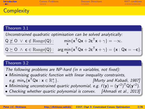
Complexity
Theorem 3.1
Unconstrained quadratic optimisation can be solved analytically:
Q � O ∨ c /∈ Range(Q) : minx{xTQx + 2cTx + γ} = −∞.
Q � O ∧ c ∈ Range(Q) : arg minx{xTQx + 2cTx + γ} = {x : Qx = −c}.
Theorem 3.2
The following problems are NP-hard (in n variables, not fixed):• Minimising quadratic function with linear inequality constraints,
e.g. minx{xTQx : x ∈ Rn+}. [Murty and Kabadi, 1987]
• Minimising unconstrained quartic polynomial, e.g. f (y) = (y◦2)TQ(y◦2).
• Checking whether quartic polynomial is convex. [Ahmadi et al., 2013]
Peter J.C. Dickinson http://dickinson.website CO17, Chpt 3: Constrained Convex Optimisation 2/26
Introduction Convex Problems Descent Directions KKT conditions
Complexity
Theorem 3.1
Unconstrained quadratic optimisation can be solved analytically:
Q � O ∨ c /∈ Range(Q) : minx{xTQx + 2cTx + γ} = −∞.
Q � O ∧ c ∈ Range(Q) : arg minx{xTQx + 2cTx + γ} = {x : Qx = −c}.
Theorem 3.2
The following problems are NP-hard (in n variables, not fixed):• Minimising quadratic function with linear inequality constraints,
e.g. minx{xTQx : x ∈ Rn+}. [Murty and Kabadi, 1987]
• Minimising unconstrained quartic polynomial, e.g. f (y) = (y◦2)TQ(y◦2).• Checking whether quartic polynomial is convex. [Ahmadi et al., 2013]
Peter J.C. Dickinson http://dickinson.website CO17, Chpt 3: Constrained Convex Optimisation 2/26
Introduction Convex Problems Descent Directions KKT conditions
Complexity Bibliography
M.R. Garey and D.S. Johnson.Computers and Intractability: A Guide to the Theory ofNP-Completeness.W.H. Freeman & Co., New York, USA, 1979.
K.G. Murty and S.N. Kabadi.Some NP-complete problems in quadratic and nonlinearprogramming.Mathematical Programming 39(2):117–129, 1987.
Amir Ali Ahmadi, Alex Olshevsky, Pablo A. Parrilo andJohn N. Tsitsiklis.NP-hardness of deciding convexity of quartic polynomials andrelated problems.Mathematical Programming 137(1-2):453–476, 2013.
Peter J.C. Dickinson http://dickinson.website CO17, Chpt 3: Constrained Convex Optimisation 3/26

Introduction Convex Problems Descent Directions KKT conditions
Literature & Survey
For further reading:
FKS: p.273 – 277
Survey: https://goo.gl/forms/eR2fJrK7nAP3vifz1
Peter J.C. Dickinson http://dickinson.website CO17, Chpt 3: Constrained Convex Optimisation 4/26

Introduction Convex Problems Descent Directions KKT conditions
Table of Contents
1 Introduction
2 Convex ProblemsUnconstrained RecapConstrainedExplicit problemActive Indices
3 Descent Directions
4 KKT conditions
Peter J.C. Dickinson http://dickinson.website CO17, Chpt 3: Constrained Convex Optimisation 5/26

Introduction Convex Problems Descent Directions KKT conditions
Optimality conditions in unconstrained optimization
infx
f (x) s. t. x ∈ C (U)
C ⊆ Rn is open set, f : C → R, f ∈ C1.
Lemma 3.3
Consider the following statements:
1 x0 is a global minimum of (U).
2 x0 is a local minimum of (U).
3 ∇f (x0) = 0.
In general we have (1)⇒ (2)⇒ (3).If f convex then (1)⇔ (2)⇔ (3).
Peter J.C. Dickinson http://dickinson.website CO17, Chpt 3: Constrained Convex Optimisation 6/26
Introduction Convex Problems Descent Directions KKT conditions
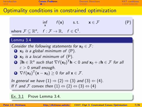
Optimality conditions in constrained optimization
infx
f (x) s. t. x ∈ F (P)
where F ⊆ Rn, f : F → R, f ∈ C1.
Lemma 3.4
Consider the following statements for x0 ∈ F :1 x0 is a global minimum of (P).2 x0 is a local minimum of (P).3 @h ∈ Rn such that ∇f (x0)Th < 0 and x0 + εh ∈ F for allε > 0 small enough.
4 ∇f (x0)T(x− x0) ≥ 0 for all x ∈ F .
In general we have (1)⇒ (2)⇒ (3) and (3)⇐ (4).If f and F convex then (1)⇔ (2)⇔ (3)⇔ (4)
Ex. 3.1 Prove Lemma 3.4.
Peter J.C. Dickinson http://dickinson.website CO17, Chpt 3: Constrained Convex Optimisation 7/26

Introduction Convex Problems Descent Directions KKT conditions
Explicit problem
infx
f (x)
s. t. gj(x) ≤ 0 for all j = 1, . . . ,m
x ∈ C.
(C)
where C ⊆ Rn is an open set, f , g1, . . . , gm ∈ C1,
F := {x ∈ C : gj(x) ≤ 0 for all j = 1, . . . ,m}
Definition 3.5
We refer to (C) as a convex (minimisation) problem if C ⊆ Rn is aconvex set and f , g1, . . . , gm are convex functions on C.
Ex. 3.2 Show that if (C) is convex problem then F is convex set.
Peter J.C. Dickinson http://dickinson.website CO17, Chpt 3: Constrained Convex Optimisation 8/26

Introduction Convex Problems Descent Directions KKT conditions
Active indices
Definition 3.6
For x ∈ F , define index i ∈ {1, . . . ,m} to be active if gi (x) = 0.Active index set Jx ⊆ {1, . . . ,m} is the set of all active indices.
Remark 3.7
If g1, . . . , gm ∈ C0 then only constraints corresponding to activeindices play a role at local minima.
Ex. 3.3 Show that if g1, . . . , gm are convex functions andx, y ∈ F then ∇gi (x)T(y − x) ≤ 0 for all i ∈ Jx.
Peter J.C. Dickinson http://dickinson.website CO17, Chpt 3: Constrained Convex Optimisation 9/26

Introduction Convex Problems Descent Directions KKT conditions
Table of Contents
1 Introduction
2 Convex Problems
3 Descent DirectionsSandwiching the conditionSlater’s ConditionConclusion so far
4 KKT conditions
Peter J.C. Dickinson http://dickinson.website CO17, Chpt 3: Constrained Convex Optimisation 10/26

Introduction Convex Problems Descent Directions KKT conditions
For fixed x0 ∈ F , when does ∃ε̂ > 0 s.t. x0 + εh ∈ F for all ε ∈ (0, ε̂]?Equivalently: ∃ε̂ > 0 s.t. gi (x0 + εh) ≤ 0 for all i and all ε ∈ (0, ε̂].Consider arbitrary i ∈ {1 . . . ,m}.
gi (x0 + εh) = gi (x0) + ε∇gi (x0)Th + o(ε).
If i /∈ Jx0 , or ∇gi (x0)Th < 0, or gi affine and ∇gi (x0)Th ≤ 0 :∃ε̂ > 0 such that gi (x0 + εh) ≤ 0 for all ε ∈ (0, ε̂].
If i ∈ Jx0 and ∇gi (x0)Th > 0:@ε̂ > 0 such that gi (x0 + εh) ≤ 0 for all ε ∈ (0, ε̂].
If i ∈ Jx0 and ∇gi (x0)Th = 0 and gi nonaffine:Condition may or may not hold.
Therefore{h ∈ Rn :
∇gi (x0)Th ≤ 0 for all i ∈ Jx0 s. t. gi affine
∇gi (x0)Th < 0 for all i ∈ Jx0 s. t. gi nonaffine
}⊆ {h ∈ Rn : ∃ε̂ > 0 s. t. x0 + εh ∈ F for all ε ∈ (0, ε̂]}
⊆ {h ∈ Rn : ∇gi (x0)Th ≤ 0 for all i ∈ Jx0}Peter J.C. Dickinson http://dickinson.website CO17, Chpt 3: Constrained Convex Optimisation 11/26

Introduction Convex Problems Descent Directions KKT conditions
Sandwiching the condition
Lemma 3.8
Consider the following statements for x0 ∈ F :
(3a) @h ∈ Rn s.t. ∇f (x0)Th < 0, ∇gi (x0)Th ≤ 0 for all i ∈ Jx0 .
(3) @h ∈ Rn such that ∇f (x0)Th < 0 and x0 + εh ∈ F for allε > 0 small enough.
(3b) @h ∈ Rn s.t. ∇f (x0)Th < 0, ∇gi (x0)Th < 0 for all i ∈ Jx0 s.t.gi is nonaffine, ∇gj(x0)Th ≤ 0 for all j ∈ Jx0 s.t. gj is affine.
In general we have (3a)⇒ (3)⇒ (3b).
When are these three statements equivalent?
Peter J.C. Dickinson http://dickinson.website CO17, Chpt 3: Constrained Convex Optimisation 12/26

Introduction Convex Problems Descent Directions KKT conditions
Slater’s Condition
Definition 3.9
We say that z ∈ Rn is a Slater point for (C) if z ∈ F andgi (z) < 0 for all i such that gi is not an affine function.
Say that Slater’s condition holds for (C) if there’s a Slater point.
Example
Consider m = n = 2, g1(x) = x21 + x22 − 4, g2(x) = x2 − 1:
Which of the following are Slater points?
A =(−2 −2
)TB =
(−1.2 −1.6
)TC =
(−0.5 −0.5
)TD =
(1 1
)TE =
(−0.5 1.5
)TF =
(−√
3 1)T
www.shakeq.com, login code utwente118
Peter J.C. Dickinson http://dickinson.website CO17, Chpt 3: Constrained Convex Optimisation 13/26

Introduction Convex Problems Descent Directions KKT conditions
Slater’s Condition
Lemma 3.10
If x0 ∈ F and problem (C) is a convex problem with Slater’scondition holding then the following are equivalent:
(3a) @h ∈ Rn s.t. ∇f (x0)Th < 0, ∇gi (x0)Th ≤ 0 for all j ∈ Jx0 .
(3) @h ∈ Rn s.t. ∇f (x0)Th < 0 and x0 + εh ∈ F for all ε > 0small enough.
(3b) @h ∈ Rn s.t. ∇f (x0)Th < 0, ∇gi (x0)Th < 0 for all i ∈ Jx0 s.t.gi is nonaffine, ∇gj(x0)Th ≤ 0 for all j ∈ Jx0 s.t. gj is affine.
Peter J.C. Dickinson http://dickinson.website CO17, Chpt 3: Constrained Convex Optimisation 14/26
Introduction Convex Problems Descent Directions KKT conditions
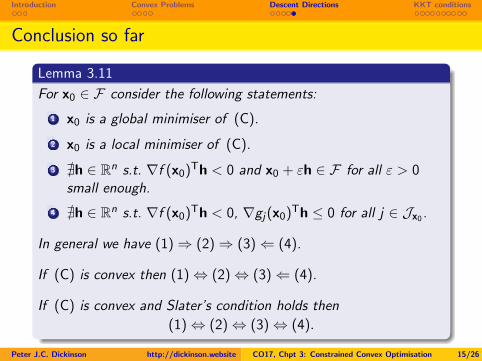
Conclusion so far
Lemma 3.11
For x0 ∈ F consider the following statements:
1 x0 is a global minimiser of (C).
2 x0 is a local minimiser of (C).
3 @h ∈ Rn s.t. ∇f (x0)Th < 0 and x0 + εh ∈ F for all ε > 0small enough.
4 @h ∈ Rn s.t. ∇f (x0)Th < 0, ∇gj(x0)Th ≤ 0 for all j ∈ Jx0 .
In general we have (1)⇒ (2)⇒ (3)⇐ (4).
If (C) is convex then (1)⇔ (2)⇔ (3)⇐ (4).
If (C) is convex and Slater’s condition holds then
(1)⇔ (2)⇔ (3)⇔ (4).
Peter J.C. Dickinson http://dickinson.website CO17, Chpt 3: Constrained Convex Optimisation 15/26

Introduction Convex Problems Descent Directions KKT conditions
Table of Contents
1 Introduction
2 Convex Problems
3 Descent Directions
4 KKT conditionsIntroductionFarkas’ LemmaExamplesExample 1More KKT examples
Peter J.C. Dickinson http://dickinson.website CO17, Chpt 3: Constrained Convex Optimisation 16/26

Introduction Convex Problems Descent Directions KKT conditions
KKT conditions
We will now consider KKT conditions.
These are important conditions for optimality in constrainedconvex optimisation problems.
Originally called Kuhn-Tucker (KT) conditions afterHarold W. Kuhn and Albert W. Tucker, who first publishedthe conditions in 1951.
Conditions later found in the 1939 Master thesis ofWilliam Karush, hence now called Karush-Kuhn-Tucker(KKT) conditions.
“Searchers find, Researchers refind.”
Peter J.C. Dickinson http://dickinson.website CO17, Chpt 3: Constrained Convex Optimisation 17/26
Introduction Convex Problems Descent Directions KKT conditions
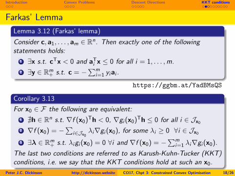
Farkas’ Lemma
Lemma 3.12 (Farkas’ lemma)
Consider c, a1, . . . , am ∈ Rn. Then exactly one of the followingstatements holds:
1 ∃x s.t. cTx < 0 and aTi x ≤ 0 for all i = 1, . . . ,m.
2 ∃y ∈ Rm+ s.t. c = −
∑mi=1 yiai .
https://ggbm.at/YadBMsQS
Corollary 3.13
For x0 ∈ F the following are equivalent:
1 @h ∈ Rn s.t. ∇f (x0)Th < 0, ∇gi (x0)Th ≤ 0 for all i ∈ Jx02 ∇f (x0) = −
∑i∈Jx0
λi∇gi (x0), for some λi ≥ 0 ∀i ∈ Jx03 ∃λ ∈ Rm
+ s.t. λigi (x0) = 0 ∀i and ∇f (x0) = −∑m
i=1 λi∇gi (x0).
The last two conditions are referred to as Karush-Kuhn-Tucker (KKT)conditions, i.e. we say that the KKT conditions hold at such an x0.
Peter J.C. Dickinson http://dickinson.website CO17, Chpt 3: Constrained Convex Optimisation 18/26

Introduction Convex Problems Descent Directions KKT conditions
Conclusion
Theorem 3.14
For x0 ∈ F consider the following statements:
1 x0 is a global minimiser of (C).
2 x0 is a local minimiser of (C).
3 @h ∈ Rn s.t. ∇f (x0)Th < 0 and x0 + εh ∈ F for all ε > 0 smallenough.
4 @h ∈ Rn s.t. ∇f (x0)Th < 0, ∇gi (x0)Th ≤ 0 for all j ∈ Jx0 .
5 ∃λ ∈ Rm+ s.t. λigi (x0) = 0 ∀i and ∇f (x0) = −
∑mi=1 λi∇gi (x0).
In general we have (1)⇒ (2)⇒ (3)⇐ (4)⇔ (5).
If (C) is convex then (1)⇔ (2)⇔ (3)⇐ (4)⇔ (5).
If (C) is convex and Slater’s condition holds then
(1)⇔ (2)⇔ (3)⇔ (4)⇔ (5).
Peter J.C. Dickinson http://dickinson.website CO17, Chpt 3: Constrained Convex Optimisation 19/26

Introduction Convex Problems Descent Directions KKT conditions
General idea to solving with KKT conditions
1 Transform to: minx{f (x) : gi (x) ≤ 0 for all i = 1, . . . ,m}.2 Analyse the problem: If the problem is convex and ...
...Slater’s cond. holds: KKT point ⇔ Global minimiser.
...Slater’s cond. doesn’t hold: KKT point ⇒: Global minimiser.
3 Find Solns (x,λ) ∈ Rn ×Rm to following system of n + m equalities:
∇f (x) = −m∑i=1
λi∇gi (x),
λi gi (x) = 0 for all i = 1, . . . ,m.
4 Solns with gi (x) ≤ 0 ∀i = 1, . . . ,m and λ ∈ Rm+ are KKT points.
[Can combine points 3 and 4.]
Peter J.C. Dickinson http://dickinson.website CO17, Chpt 3: Constrained Convex Optimisation 20/26

Introduction Convex Problems Descent Directions KKT conditions
Example 1: Steps 1 & 2: Transform & Analyse problem
For parameter a ∈ R consider problem
minx{2x1 + ax2 : x2 ≤ 1, x21 ≤ x2}.
f (x) = 2x1 + ax2, ∇f =
(2a
), ∇2f =
(0 00 0
)⇒ Affine function
g1(x) = x2 − 1, ∇g1 =
(01
), ∇2g1 =
(0 00 0
)⇒ Affine function
g2(x) = x21 − x2, ∇g2 =
(2x1−1
), ∇2g2 =
(2 00 0
)⇒ Convex function
Therefore convex minimisation problem.g2 is the only nonaffine constraint function, and for x = (0, 1) ∈ Fhave g2(x) = −1 < 0. Therefore Slater’s condition holds.Therefore a point is global minimiser if and only if it is KKT point.
Peter J.C. Dickinson http://dickinson.website CO17, Chpt 3: Constrained Convex Optimisation 21/26
Introduction Convex Problems Descent Directions KKT conditions
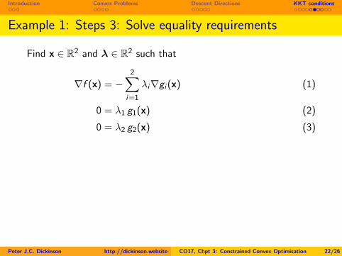
Example 1: Steps 3: Solve equality requirements
Find x ∈ R2 and λ ∈ R2 such that
(2a
)=
∇f (x) = −2∑
i=1
λi∇gi (x)
= −λ1(
01
)− λ2
(2x1−1
)
(1)
0 = λ1 g1(x)
= λ1(x2 − 1)
(2)
0 = λ2 g2(x)
= λ2(x21 − x2)
(3)
Solution to (1) ⇔ λ2 6= 0 and x1 = −λ−12 and λ1 = λ2 − a.As require λ2 ≥ 0, can restrict to λ2 > 0 > x1.As λ2 > 0, solution to (3) ⇔ x2 = x21 = λ−22 .Two possible ways to satisfy (2):
λ1 = 0: Then x =(??, ??
)Tand λ =
(0, ??
)T.
x2 = 1: Then x =(??, 1
)Tand λ =
(??, ??
)T.
Peter J.C. Dickinson http://dickinson.website CO17, Chpt 3: Constrained Convex Optimisation 22/26
Introduction Convex Problems Descent Directions KKT conditions
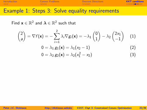
Example 1: Steps 3: Solve equality requirements
Find x ∈ R2 and λ ∈ R2 such that(2a
)= ∇f (x) = −
2∑i=1
λi∇gi (x) = −λ1(
01
)− λ2
(2x1−1
)(1)
0 = λ1 g1(x) = λ1(x2 − 1) (2)
0 = λ2 g2(x) = λ2(x21 − x2) (3)
Solution to (1) ⇔ λ2 6= 0 and x1 = −λ−12 and λ1 = λ2 − a.As require λ2 ≥ 0, can restrict to λ2 > 0 > x1.As λ2 > 0, solution to (3) ⇔ x2 = x21 = λ−22 .Two possible ways to satisfy (2):
λ1 = 0: Then x =(??, ??
)Tand λ =
(0, ??
)T.
x2 = 1: Then x =(??, 1
)Tand λ =
(??, ??
)T.
Peter J.C. Dickinson http://dickinson.website CO17, Chpt 3: Constrained Convex Optimisation 22/26

Introduction Convex Problems Descent Directions KKT conditions
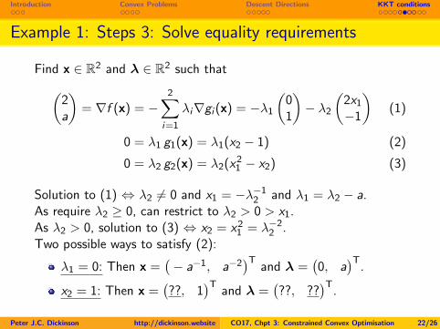
Example 1: Steps 3: Solve equality requirements
Find x ∈ R2 and λ ∈ R2 such that(2a
)= ∇f (x) = −
2∑i=1
λi∇gi (x) = −λ1(
01
)− λ2
(2x1−1
)(1)
0 = λ1 g1(x) = λ1(x2 − 1) (2)
0 = λ2 g2(x) = λ2(x21 − x2) (3)
Solution to (1) ⇔ λ2 6= 0 and x1 = −λ−12 and λ1 = λ2 − a.As require λ2 ≥ 0, can restrict to λ2 > 0 > x1.As λ2 > 0, solution to (3) ⇔ x2 = x21 = λ−22 .Two possible ways to satisfy (2):
λ1 = 0: Then x =(??, ??
)Tand λ =
(0, a
)T.
x2 = 1: Then x =(??, 1
)Tand λ =
(??, ??
)T.
Peter J.C. Dickinson http://dickinson.website CO17, Chpt 3: Constrained Convex Optimisation 22/26
Introduction Convex Problems Descent Directions KKT conditions
Example 1: Steps 3: Solve equality requirements
Find x ∈ R2 and λ ∈ R2 such that(2a
)= ∇f (x) = −
2∑i=1
λi∇gi (x) = −λ1(
01
)− λ2
(2x1−1
)(1)
0 = λ1 g1(x) = λ1(x2 − 1) (2)
0 = λ2 g2(x) = λ2(x21 − x2) (3)
Solution to (1) ⇔ λ2 6= 0 and x1 = −λ−12 and λ1 = λ2 − a.As require λ2 ≥ 0, can restrict to λ2 > 0 > x1.As λ2 > 0, solution to (3) ⇔ x2 = x21 = λ−22 .Two possible ways to satisfy (2):
λ1 = 0: Then x =(− a−1, a−2
)Tand λ =
(0, a
)T.
x2 = 1: Then x =(??, 1
)Tand λ =
(??, ??
)T.
Peter J.C. Dickinson http://dickinson.website CO17, Chpt 3: Constrained Convex Optimisation 22/26

Introduction Convex Problems Descent Directions KKT conditions
Example 1: Steps 3: Solve equality requirements
Find x ∈ R2 and λ ∈ R2 such that(2a
)= ∇f (x) = −
2∑i=1
λi∇gi (x) = −λ1(
01
)− λ2
(2x1−1
)(1)
0 = λ1 g1(x) = λ1(x2 − 1) (2)
0 = λ2 g2(x) = λ2(x21 − x2) (3)
Solution to (1) ⇔ λ2 6= 0 and x1 = −λ−12 and λ1 = λ2 − a.As require λ2 ≥ 0, can restrict to λ2 > 0 > x1.As λ2 > 0, solution to (3) ⇔ x2 = x21 = λ−22 .Two possible ways to satisfy (2):
λ1 = 0: Then x =(− a−1, a−2
)Tand λ =
(0, a
)T.
x2 = 1: Then x =(− 1, 1
)Tand λ =
(??, 1
)T.
Peter J.C. Dickinson http://dickinson.website CO17, Chpt 3: Constrained Convex Optimisation 22/26

Introduction Convex Problems Descent Directions KKT conditions
Example 1: Steps 3: Solve equality requirements
Find x ∈ R2 and λ ∈ R2 such that(2a
)= ∇f (x) = −
2∑i=1
λi∇gi (x) = −λ1(
01
)− λ2
(2x1−1
)(1)
0 = λ1 g1(x) = λ1(x2 − 1) (2)
0 = λ2 g2(x) = λ2(x21 − x2) (3)
Solution to (1) ⇔ λ2 6= 0 and x1 = −λ−12 and λ1 = λ2 − a.As require λ2 ≥ 0, can restrict to λ2 > 0 > x1.As λ2 > 0, solution to (3) ⇔ x2 = x21 = λ−22 .Two possible ways to satisfy (2):
λ1 = 0: Then x =(− a−1, a−2
)Tand λ =
(0, a
)T.
x2 = 1: Then x =(− 1, 1
)Tand λ =
(1− a, 1
)T.
Peter J.C. Dickinson http://dickinson.website CO17, Chpt 3: Constrained Convex Optimisation 22/26

Introduction Convex Problems Descent Directions KKT conditions
Example 1: Steps 4: Check inequality requirements
Have 2 candidate solutions, which fulfill all the KKT equalityrequirements. Will now check the inequality requirements:
x =(−a−1, a−2
)Tand λ =
(0, a
)T:
Require a 6= 0, otherwise solution ill defined.
Have λ ∈ R2+ ⇔ a ≥ 0.
g2(x) = x21 − x2 = 0.g1(x) = x2 − 1 = a−2 − 1. Have g1(x) ≤ 0⇔ |a| ≥ 1.
Inequalities satisfied if and only if a ≥ 1.
x =(−1, 1
)Tand λ =
(1− a, 1
)T:
Have λ ∈ R2+ ⇔ a ≤ 1.
g1(x) = x2 − 1 = 0 and g2(x) = x21 − x2 = 0.
Inequalities satisfied if and only if a ≤ 1.
N.B. If a = 1 for both have x =(−1, 1
)Tand λ =
(0, 1
)T.
Peter J.C. Dickinson http://dickinson.website CO17, Chpt 3: Constrained Convex Optimisation 23/26

Introduction Convex Problems Descent Directions KKT conditions
Example 1: Conclusion
If a ≤ 1 have unique global minimiser at x∗ =(−1, 1
)T.
This corresponds to λ∗ =(1− a, 1
)T.
Both constraints are active.
Optimal value equals f (x∗) = −2 + a.
If a > 1 have unique global minimiser at x∗ =(−a−1, a−2
)T.
This corresponds to λ∗ =(0, a
)T.
Only the second constraint is active.
Optimal value equals f (x∗) = −2a−1 + aa−2 = −a−1.
Peter J.C. Dickinson http://dickinson.website CO17, Chpt 3: Constrained Convex Optimisation 24/26

Introduction Convex Problems Descent Directions KKT conditions
KKT examples
Example
minx{x2 : (x − 2)2 ≤ 1}
Example
minx{x2 : (x − 2)2 ≤ 9} (can have Jx = ∅ at minimum)
Example
minx{x2 : (x − 2)2 ≤ 0} (KKT conditions not necessary)
Example
For c, a ∈ Rn with c 6= 0 consider the problem
minx{cTx : ‖x− a‖22 ≤ 1}
Peter J.C. Dickinson http://dickinson.website CO17, Chpt 3: Constrained Convex Optimisation 25/26
Introduction Convex Problems Descent Directions KKT conditions
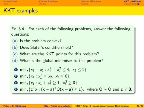
KKT examples
Ex. 3.4 For each of the following problems, answer the followingquestions:
(a) Is the problem convex?
(b) Does Slater’s condition hold?
(c) What are the KKT points for this problem?
(d) What is the global minimiser to this problem?
1 minx{x1 − x2 : x21 + x22 ≤ 4, x2 ≤ 1};2 minx{x1 : x21 ≤ x2, x2 ≤ 0};3 minx{x1 : x1 + x22 ≥ 1, x31 ≥ 0};4 minx{cTx : (x− a)TQ(x− a) ≤ 1}, where Q � O and c 6= 0.
Peter J.C. Dickinson http://dickinson.website CO17, Chpt 3: Constrained Convex Optimisation 26/26