Embed Size (px)
Citation preview

Continuous Facility LocationAlgorithms for k-Means and k-Median
Nathan Cordner
Boston University
4 November 2019
Cordner (Boston University) 4 November 2019 Continuous FL Algorithms

Clustering Problems
Given discrete subsets C and F of metric space (X, d)
k-Median problem:Choose k centers in FMinimize distances from each point in C to its nearestcenter
k-Means problem:Choose k centers within XMinimize squared distances from each point in C to itsnearest centerCan discretize the possible choices for centers withnegligible approximation loss
Cordner (Boston University) 4 November 2019 Continuous FL Algorithms

Clustering Problems
Given discrete subsets C and F of metric space (X, d)k-Median problem:
Choose k centers in FMinimize distances from each point in C to its nearestcenter
k-Means problem:Choose k centers within XMinimize squared distances from each point in C to itsnearest centerCan discretize the possible choices for centers withnegligible approximation loss
Cordner (Boston University) 4 November 2019 Continuous FL Algorithms

Clustering Problems
Given discrete subsets C and F of metric space (X, d)k-Median problem:
Choose k centers in F
Minimize distances from each point in C to its nearestcenter
k-Means problem:Choose k centers within XMinimize squared distances from each point in C to itsnearest centerCan discretize the possible choices for centers withnegligible approximation loss
Cordner (Boston University) 4 November 2019 Continuous FL Algorithms

Clustering Problems
Given discrete subsets C and F of metric space (X, d)k-Median problem:
Choose k centers in FMinimize distances from each point in C to its nearestcenter
k-Means problem:Choose k centers within XMinimize squared distances from each point in C to itsnearest centerCan discretize the possible choices for centers withnegligible approximation loss
Cordner (Boston University) 4 November 2019 Continuous FL Algorithms

Clustering Problems
Given discrete subsets C and F of metric space (X, d)k-Median problem:
Choose k centers in FMinimize distances from each point in C to its nearestcenter
k-Means problem:
Choose k centers within XMinimize squared distances from each point in C to itsnearest centerCan discretize the possible choices for centers withnegligible approximation loss
Cordner (Boston University) 4 November 2019 Continuous FL Algorithms

Clustering Problems
Given discrete subsets C and F of metric space (X, d)k-Median problem:
Choose k centers in FMinimize distances from each point in C to its nearestcenter
k-Means problem:Choose k centers within X
Minimize squared distances from each point in C to itsnearest centerCan discretize the possible choices for centers withnegligible approximation loss
Cordner (Boston University) 4 November 2019 Continuous FL Algorithms

Clustering Problems
Given discrete subsets C and F of metric space (X, d)k-Median problem:
Choose k centers in FMinimize distances from each point in C to its nearestcenter
k-Means problem:Choose k centers within XMinimize squared distances from each point in C to itsnearest center
Can discretize the possible choices for centers withnegligible approximation loss
Cordner (Boston University) 4 November 2019 Continuous FL Algorithms

Clustering Problems
Given discrete subsets C and F of metric space (X, d)k-Median problem:
Choose k centers in FMinimize distances from each point in C to its nearestcenter
k-Means problem:Choose k centers within XMinimize squared distances from each point in C to itsnearest centerCan discretize the possible choices for centers withnegligible approximation loss
Cordner (Boston University) 4 November 2019 Continuous FL Algorithms

Approximation Bounds Overview
k-Median:
2001: Jain and Vazirani 6-approx.
2002: Jain et al. 4-approx.
2003: Archer et al. exponential 3-approx.
2012: Li and Svensson 2.732-approx.
2014: Byrka et al. 2.675-approx.
2017: Ahmadian et al. 2.633-approx. (Euclidean)
Hardness: 1.736
Cordner (Boston University) 4 November 2019 Continuous FL Algorithms

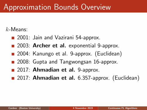
Approximation Bounds Overview
k-Means:
2001: Jain and Vazirani 54-approx.
2003: Archer et al. exponential 9-approx.
2004: Kanungo et al. 9-approx. (Euclidean)
2008: Gupta and Tangwongsan 16-approx.
2017: Ahmadian et al. 9-approx.
2017: Ahmadian et al. 6.357-approx. (Euclidean)
Hardness: 3.94 (General), 1.0013 (Euclidean)
Cordner (Boston University) 4 November 2019 Continuous FL Algorithms

Talk Outline
Facility Location Problem
Jain and Vazirani (JV) Algorithm
Relation to k-Means and k-Median
Continuous Adaptations of the JV Algorithm
Archer et al. Exponential Algorithm
Ahmadian et al. Quasipolynomial Algorithm
Ahmadian et al. Polynomial Algorithm
Cordner (Boston University) 4 November 2019 Continuous FL Algorithms

Uncapacitated Facility Location
Figure: researchgate.net/figure/Facility-location-problem-example fig1 221182599
Cordner (Boston University) 4 November 2019 Continuous FL Algorithms

Uncapacitated Facility Location
Given a set of facilities F , and a set of clients C
Each facility i has an opening cost
Want to minimize facility opening costs plusdistances of clients to their nearest facility
Cordner (Boston University) 4 November 2019 Continuous FL Algorithms

Uncapacitated Facility Location
Given a set of facilities F , and a set of clients C
Each facility i has an opening cost
Want to minimize facility opening costs plusdistances of clients to their nearest facility
Cordner (Boston University) 4 November 2019 Continuous FL Algorithms

Uncapacitated Facility Location
Given a set of facilities F , and a set of clients C
Each facility i has an opening cost
Want to minimize facility opening costs plusdistances of clients to their nearest facility
Cordner (Boston University) 4 November 2019 Continuous FL Algorithms

Uncapacitated Facility Location
Primal LP:
minimize∑
i∈F,j∈Ccijxij +
∑i∈F
fiyi
subject to∑i∈F
xij ≥ 1, ∀j ∈ C,
yi − xij ≥ 0, ∀i ∈ F, j ∈ C,
xij ≥ 0, ∀i ∈ F, j ∈ C,
yi ≥ 0, ∀i ∈ F.
cij = distance, fi = facility cost,xij = client connection, yi = facility open
Cordner (Boston University) 4 November 2019 Continuous FL Algorithms

Uncapacitated Facility Location
Dual LP:
maximize∑j∈C
αj
subject to αj − βij ≤ cij, ∀i ∈ F, j ∈ C,∑j∈C
βij ≤ fi, ∀i ∈ F,
αj ≥ 0, ∀j ∈ C,
βij ≥ 0, ∀i ∈ F, j ∈ C.
cij = distance, fi = facility cost,βij = client contribution, αj = client value
Cordner (Boston University) 4 November 2019 Continuous FL Algorithms

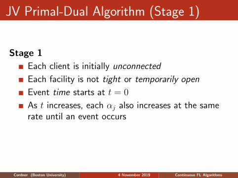
JV Primal-Dual Algorithm (Stage 1)
Stage 1
Each client is initially unconnected
Each facility is not tight or temporarily open
Event time starts at t = 0
As t increases, each αj also increases at the samerate until an event occurs
Stage 1 ends when no unconnected clients remain
Cordner (Boston University) 4 November 2019 Continuous FL Algorithms

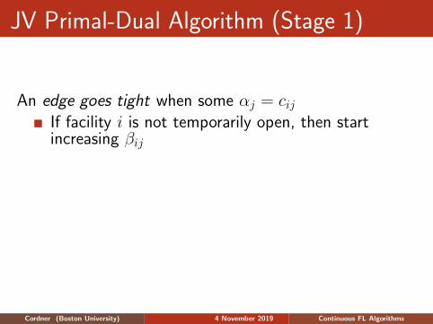
JV Primal-Dual Algorithm (Stage 1)
An edge goes tight when some αj = cij
If facility i is not temporarily open, then startincreasing βij
Client j is now contributing to facility i
If facility i is temporarily open, then declare client jto be connected
Stop increasing αj and each βhj for all facilities h ∈ FFacility i is the connecting witness for client j
Cordner (Boston University) 4 November 2019 Continuous FL Algorithms
JV Primal-Dual Algorithm (Stage 1)
An edge goes tight when some αj = cijIf facility i is not temporarily open, then startincreasing βij
Client j is now contributing to facility i
If facility i is temporarily open, then declare client jto be connected
Stop increasing αj and each βhj for all facilities h ∈ FFacility i is the connecting witness for client j
Cordner (Boston University) 4 November 2019 Continuous FL Algorithms

JV Primal-Dual Algorithm (Stage 1)
An edge goes tight when some αj = cijIf facility i is not temporarily open, then startincreasing βij
Client j is now contributing to facility i
If facility i is temporarily open, then declare client jto be connected
Stop increasing αj and each βhj for all facilities h ∈ F
Facility i is the connecting witness for client j
Cordner (Boston University) 4 November 2019 Continuous FL Algorithms

JV Primal-Dual Algorithm (Stage 1)
An edge goes tight when some αj = cijIf facility i is not temporarily open, then startincreasing βij
Client j is now contributing to facility i
If facility i is temporarily open, then declare client jto be connected
Stop increasing αj and each βhj for all facilities h ∈ FFacility i is the connecting witness for client j
Cordner (Boston University) 4 November 2019 Continuous FL Algorithms

JV Primal-Dual Algorithm (Stage 1)
Facility i is paid for when∑
j∈C βij = fi
Declare facility i to be temporarily open
Each unconnected client j that was contributing tofacility i is now declared to be connected
Facility i is the connecting witness for these clients
The dual variables for each of these clients nowstops increasing
Cordner (Boston University) 4 November 2019 Continuous FL Algorithms
JV Primal-Dual Algorithm (Stage 1)
Facility i is paid for when∑
j∈C βij = fiDeclare facility i to be temporarily open
Each unconnected client j that was contributing tofacility i is now declared to be connected
Facility i is the connecting witness for these clients
The dual variables for each of these clients nowstops increasing
Cordner (Boston University) 4 November 2019 Continuous FL Algorithms
JV Primal-Dual Algorithm (Stage 2)
Stage 2
Construct a graph G with vertices given by thetemporarily opened facilities from Stage 1
Allow an edge between facilities i 6= i′ if some clientj made positive contributions to both
Return any maximal independent set of G
Cordner (Boston University) 4 November 2019 Continuous FL Algorithms

Relating UFL to k-Median and k-Means
JV Algorithm Approximation Bound:∑i∈F,j∈C
cijxij +∑i∈F
fiyi ≤ 3∑j∈C
αj
The JV algorithm also satisfies a Lagrange-multiplierpreserving (LMP) property:∑
i∈F,j∈C
cijxij + 3∑i∈F
fiyi ≤ 3∑j∈C
αj
Cordner (Boston University) 4 November 2019 Continuous FL Algorithms

Relating UFL to k-Median and k-Means
JV Algorithm Approximation Bound:∑i∈F,j∈C
cijxij +∑i∈F
fiyi ≤ 3∑j∈C
αj
The JV algorithm also satisfies a Lagrange-multiplierpreserving (LMP) property:∑
i∈F,j∈C
cijxij + 3∑i∈F
fiyi ≤ 3∑j∈C
αj
Cordner (Boston University) 4 November 2019 Continuous FL Algorithms
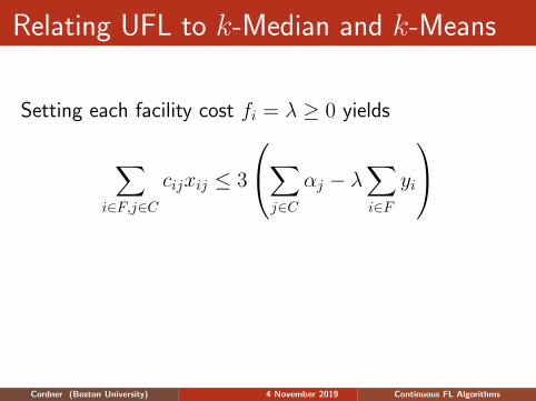
Relating UFL to k-Median and k-Means
Setting each facility cost fi = λ ≥ 0 yields
∑i∈F,j∈C
cijxij ≤ 3
∑j∈C
αj − λ∑i∈F
yi
This corresponds to the primal and dual objectives ofk-median when the number of opened facilities equals k
Bound for (discrete) k-means is 9
Cordner (Boston University) 4 November 2019 Continuous FL Algorithms

JV Algorithm Continuity
Given a UFL instance with uniform facility cost λ ≥ 0
When λ = 0, all facilities open
When λ is large enough, only one facility opens
The JV algorithm is continuous if, as λ increases,the total number of opened facilities never jumps bymore than 1 at a time
Cordner (Boston University) 4 November 2019 Continuous FL Algorithms

JV Algorithm Continuity
A bad example:
Figure: https://en.wikipedia.org/wiki/Star (graph theory)
Cordner (Boston University) 4 November 2019 Continuous FL Algorithms
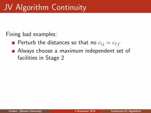
JV Algorithm Continuity
Fixing bad examples:
Perturb the distances so that no cij = ci′j′
Always choose a maximum independent set offacilities in Stage 2
Theorem (Archer et al.): as λ increases, the number ofopened facilities changes by at most 1 at a time
Exponential time algorithm
Cordner (Boston University) 4 November 2019 Continuous FL Algorithms

A New Approach
Instead of choosing maximum IS, we will just allow for“larger” maximal IS
Let ti be the time that facility i opens in Stage 1
Stage 2: edge between facilities i, i′ if some clienthas positive contributions to both and ifcii′ ≤ δmin{ti, ti′}
Note that δ =∞ yields the original JV algorithm
Cordner (Boston University) 4 November 2019 Continuous FL Algorithms

LMP Properties of JV(δ)
The JV(δ) algorithm satisfies the LMP property withconstant
9 for k-means in general metrics (δ =∞)
6.3574 for k-means in the Euclidean metric(δ = 2.3146)
3 for k-median in general metrics (δ =∞)
2.633 for k-median in the Euclidean metric(δ = 1.633)
Cordner (Boston University) 4 November 2019 Continuous FL Algorithms

LMP Analysis
Consider JV(∞) for k-median:
Given a maximal independent set IS of facilities
Let i be the witness facility for some client j
If i ∈ IS, the distance cij is bounded by αjIf i /∈ IS, then some client j’ contributed to both iand some i′ ∈ IS: ci′j ≤ cij + cij′ + ci′j′ ≤ 3αjLeads to overall 3-approximation result
Cordner (Boston University) 4 November 2019 Continuous FL Algorithms

LMP Analysis
Consider JV(∞) for k-median:
Given a maximal independent set IS of facilities
Let i be the witness facility for some client j
If i ∈ IS, the distance cij is bounded by αj
If i /∈ IS, then some client j’ contributed to both iand some i′ ∈ IS: ci′j ≤ cij + cij′ + ci′j′ ≤ 3αjLeads to overall 3-approximation result
Cordner (Boston University) 4 November 2019 Continuous FL Algorithms

LMP Analysis
Consider JV(∞) for k-median:
Given a maximal independent set IS of facilities
Let i be the witness facility for some client j
If i ∈ IS, the distance cij is bounded by αjIf i /∈ IS, then some client j’ contributed to both iand some i′ ∈ IS: ci′j ≤ cij + cij′ + ci′j′ ≤ 3αj
Leads to overall 3-approximation result
Cordner (Boston University) 4 November 2019 Continuous FL Algorithms

LMP Analysis
Consider JV(∞) for k-median:
Given a maximal independent set IS of facilities
Let i be the witness facility for some client j
If i ∈ IS, the distance cij is bounded by αjIf i /∈ IS, then some client j’ contributed to both iand some i′ ∈ IS: ci′j ≤ cij + cij′ + ci′j′ ≤ 3αjLeads to overall 3-approximation result
Cordner (Boston University) 4 November 2019 Continuous FL Algorithms
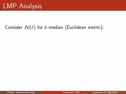
LMP Analysis
Consider JV(δ) for k-median (Euclidean metric):
Let ρ be our approximation bound
Now j may have contributed to s > 1 facilities in IS
A centroid inequality yields s < δ2/(δ2 − 2)
If s = 0, then ρ ≥ 1 + δ
If s > 1, then ρ ≥ 1/(
1s−1(s2
)δ − (s− 1)
)Best result: δ =
√8/3 yields s < 4 and ρ ≈ 2.633
Cordner (Boston University) 4 November 2019 Continuous FL Algorithms

LMP Analysis
Consider JV(δ) for k-median (Euclidean metric):
Let ρ be our approximation bound
Now j may have contributed to s > 1 facilities in IS
A centroid inequality yields s < δ2/(δ2 − 2)
If s = 0, then ρ ≥ 1 + δ
If s > 1, then ρ ≥ 1/(
1s−1(s2
)δ − (s− 1)
)
Best result: δ =√8/3 yields s < 4 and ρ ≈ 2.633
Cordner (Boston University) 4 November 2019 Continuous FL Algorithms

LMP Analysis
Consider JV(δ) for k-median (Euclidean metric):
Let ρ be our approximation bound
Now j may have contributed to s > 1 facilities in IS
A centroid inequality yields s < δ2/(δ2 − 2)
If s = 0, then ρ ≥ 1 + δ
If s > 1, then ρ ≥ 1/(
1s−1(s2
)δ − (s− 1)
)Best result: δ =
√8/3 yields s < 4 and ρ ≈ 2.633
Cordner (Boston University) 4 November 2019 Continuous FL Algorithms
Quasipolynomial Algorithm
Goal: find “good, close” dual solutions α(0), . . . , α(L)
We also control the change in number of openfacilities between solutions
Parameter values λ = 0, εz, 2εz, . . . , LεzLet ε be an approximation error factor, let n = |C|Fix εz = n−3−30 log1+ε n, L = 4n7 · ε−1z = nO(ε−1 log n)
List is quasipolynomial in length
Two parts: QuasiSweep, QuasiGraphUpdate
Cordner (Boston University) 4 November 2019 Continuous FL Algorithms

Quasipolynomial Algorithm
Goal: find “good, close” dual solutions α(0), . . . , α(L)
We also control the change in number of openfacilities between solutions
Parameter values λ = 0, εz, 2εz, . . . , Lεz
Let ε be an approximation error factor, let n = |C|Fix εz = n−3−30 log1+ε n, L = 4n7 · ε−1z = nO(ε−1 log n)
List is quasipolynomial in length
Two parts: QuasiSweep, QuasiGraphUpdate
Cordner (Boston University) 4 November 2019 Continuous FL Algorithms

Quasipolynomial Algorithm
Goal: find “good, close” dual solutions α(0), . . . , α(L)
We also control the change in number of openfacilities between solutions
Parameter values λ = 0, εz, 2εz, . . . , LεzLet ε be an approximation error factor, let n = |C|
Fix εz = n−3−30 log1+ε n, L = 4n7 · ε−1z = nO(ε−1 log n)
List is quasipolynomial in length
Two parts: QuasiSweep, QuasiGraphUpdate
Cordner (Boston University) 4 November 2019 Continuous FL Algorithms
Quasipolynomial Algorithm
Goal: find “good, close” dual solutions α(0), . . . , α(L)
We also control the change in number of openfacilities between solutions
Parameter values λ = 0, εz, 2εz, . . . , LεzLet ε be an approximation error factor, let n = |C|Fix εz = n−3−30 log1+ε n, L = 4n7 · ε−1z = nO(ε−1 log n)
List is quasipolynomial in length
Two parts: QuasiSweep, QuasiGraphUpdate
Cordner (Boston University) 4 November 2019 Continuous FL Algorithms

Quasipolynomial Algorithm
Goal: find “good, close” dual solutions α(0), . . . , α(L)
We also control the change in number of openfacilities between solutions
Parameter values λ = 0, εz, 2εz, . . . , LεzLet ε be an approximation error factor, let n = |C|Fix εz = n−3−30 log1+ε n, L = 4n7 · ε−1z = nO(ε−1 log n)
List is quasipolynomial in length
Two parts: QuasiSweep, QuasiGraphUpdate
Cordner (Boston University) 4 November 2019 Continuous FL Algorithms

QuasiSweep
For x ∈ R, define
B(x) =
{0, if x < 1,1 + blog1+ε(x)c, if x ≥ 1
B(x) is the index of the bucket that contains x
The α-values for any two clients in the same bucketdiffer by at most 1 + ε
Cordner (Boston University) 4 November 2019 Continuous FL Algorithms

QuasiSweep
For x ∈ R, define
B(x) =
{0, if x < 1,1 + blog1+ε(x)c, if x ≥ 1
B(x) is the index of the bucket that contains x
The α-values for any two clients in the same bucketdiffer by at most 1 + ε
Cordner (Boston University) 4 November 2019 Continuous FL Algorithms

QuasiSweep
For x ∈ R, define
B(x) =
{0, if x < 1,1 + blog1+ε(x)c, if x ≥ 1
B(x) is the index of the bucket that contains x
The α-values for any two clients in the same bucketdiffer by at most 1 + ε
Cordner (Boston University) 4 November 2019 Continuous FL Algorithms

QuasiSweep
Begin with good dual solution α(l) for parameter λ
Raise the facility price to λ+ εzLet A = ∅ and θ = 0. Increase θ continuously:
Whenever θ = αj, add j to A
Remove j from A whenever j has a tight edge to atight facility i where B(αj) ≥ B(ti)
Decrease each αj with B(αj) > B(θ) at a rate of|A| times the rate that θ is increasing
Stop when every client is added and removed from AOutput dual solution α(l+1) for parameter λ+ εz
Cordner (Boston University) 4 November 2019 Continuous FL Algorithms
QuasiSweep
Begin with good dual solution α(l) for parameter λ
Raise the facility price to λ+ εz
Let A = ∅ and θ = 0. Increase θ continuously:
Whenever θ = αj, add j to A
Remove j from A whenever j has a tight edge to atight facility i where B(αj) ≥ B(ti)
Decrease each αj with B(αj) > B(θ) at a rate of|A| times the rate that θ is increasing
Stop when every client is added and removed from AOutput dual solution α(l+1) for parameter λ+ εz
Cordner (Boston University) 4 November 2019 Continuous FL Algorithms

QuasiSweep
Begin with good dual solution α(l) for parameter λ
Raise the facility price to λ+ εzLet A = ∅ and θ = 0. Increase θ continuously:
Whenever θ = αj, add j to A
Remove j from A whenever j has a tight edge to atight facility i where B(αj) ≥ B(ti)
Decrease each αj with B(αj) > B(θ) at a rate of|A| times the rate that θ is increasing
Stop when every client is added and removed from AOutput dual solution α(l+1) for parameter λ+ εz
Cordner (Boston University) 4 November 2019 Continuous FL Algorithms

QuasiSweep
Begin with good dual solution α(l) for parameter λ
Raise the facility price to λ+ εzLet A = ∅ and θ = 0. Increase θ continuously:
Whenever θ = αj, add j to A
Remove j from A whenever j has a tight edge to atight facility i where B(αj) ≥ B(ti)
Decrease each αj with B(αj) > B(θ) at a rate of|A| times the rate that θ is increasing
Stop when every client is added and removed from A
Output dual solution α(l+1) for parameter λ+ εz
Cordner (Boston University) 4 November 2019 Continuous FL Algorithms

QuasiSweep
Begin with good dual solution α(l) for parameter λ
Raise the facility price to λ+ εzLet A = ∅ and θ = 0. Increase θ continuously:
Whenever θ = αj, add j to A
Remove j from A whenever j has a tight edge to atight facility i where B(αj) ≥ B(ti)
Decrease each αj with B(αj) > B(θ) at a rate of|A| times the rate that θ is increasing
Stop when every client is added and removed from AOutput dual solution α(l+1) for parameter λ+ εz
Cordner (Boston University) 4 November 2019 Continuous FL Algorithms

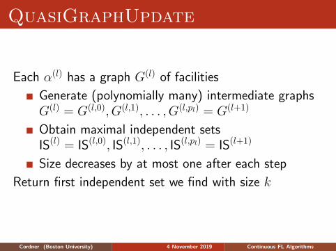
QuasiGraphUpdate
Each α(l) has a graph G(l) of facilities
Generate (polynomially many) intermediate graphsG(l) = G(l,0), G(l,1), . . . , G(l,pl) = G(l+1)
Obtain maximal independent setsIS(l) = IS(l,0), IS(l,1), . . . , IS(l,pl) = IS(l+1)
Size decreases by at most one after each step
Return first independent set we find with size k
Cordner (Boston University) 4 November 2019 Continuous FL Algorithms
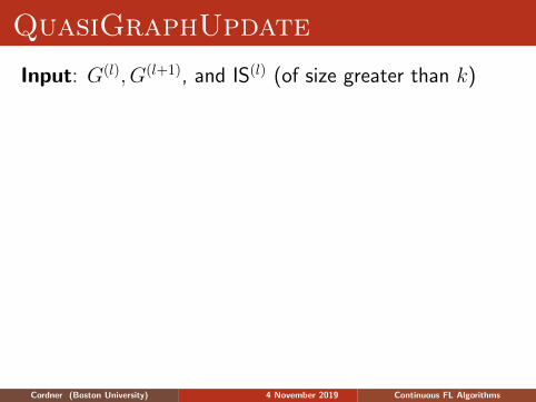
QuasiGraphUpdate
Input: G(l), G(l+1), and IS(l) (of size greater than k)
Copy G(l), G(l+1) into disjoint sets V (l), V (l+1)
Bipartite graph G′ over V (l) ∪ V (l+1) and C
Edge j to i ∈ V (l) if j contributes to i in α(l), etc.
Generate G(l,1) on G′, where the induced subgraphof G(l,1) on V (l) equals G(l) = G(l,0)
Greedily extend IS(l) = IS(l,0) to a maximalindependent set IS(l,1) for G(l,1)
Continue generating graphs and IS’s by removingfacilities in V (l) from G′ one by one
After pl = |V (l)| steps, arrive at G(l,pl) = G(l+1)
Cordner (Boston University) 4 November 2019 Continuous FL Algorithms

Quasipolynomial Algorithm: in Review
QuasiSweep generates a quasipolynomial length list ofdual solutions α(0), . . . , α(L)
QuasiGraphUpdate interpolates between every twosolutions α(l), α(l+1) to make sure we eventually find aset of open facilities of size k
Analysis:∑
i∈F,j∈Ccijxij ≤ (ρ+O(ε)) · OPTk
Cordner (Boston University) 4 November 2019 Continuous FL Algorithms

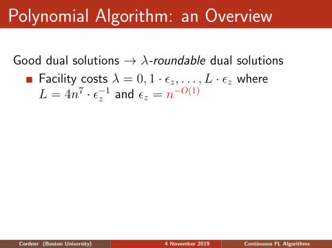
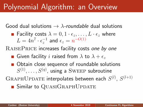
Polynomial Algorithm: an Overview
Good dual solutions → λ-roundable dual solutions
Facility costs λ = 0, 1 · εz, . . . , L · εz whereL = 4n7 · ε−1z and εz = n−O(1)
RaisePrice increases facility costs one by one
Given facility i raised from λ to λ+ εzObtain close sequence of roundable solutionsS(1), . . . , S(q), using a Sweep subroutine
GraphUpdate interpolates between each S(l), S(l+1)
Similar to QuasiGraphUpdate
Cordner (Boston University) 4 November 2019 Continuous FL Algorithms

Polynomial Algorithm: an Overview
Good dual solutions → λ-roundable dual solutions
Facility costs λ = 0, 1 · εz, . . . , L · εz whereL = 4n7 · ε−1z and εz = n−O(1)
RaisePrice increases facility costs one by one
Given facility i raised from λ to λ+ εz
Obtain close sequence of roundable solutionsS(1), . . . , S(q), using a Sweep subroutine
GraphUpdate interpolates between each S(l), S(l+1)
Similar to QuasiGraphUpdate
Cordner (Boston University) 4 November 2019 Continuous FL Algorithms

Polynomial Algorithm: an Overview
Good dual solutions → λ-roundable dual solutions
Facility costs λ = 0, 1 · εz, . . . , L · εz whereL = 4n7 · ε−1z and εz = n−O(1)
RaisePrice increases facility costs one by one
Given facility i raised from λ to λ+ εzObtain close sequence of roundable solutionsS(1), . . . , S(q), using a Sweep subroutine
GraphUpdate interpolates between each S(l), S(l+1)
Similar to QuasiGraphUpdate
Cordner (Boston University) 4 November 2019 Continuous FL Algorithms

Polynomial Algorithm: an Overview
Good dual solutions → λ-roundable dual solutions
Facility costs λ = 0, 1 · εz, . . . , L · εz whereL = 4n7 · ε−1z and εz = n−O(1)
RaisePrice increases facility costs one by one
Given facility i raised from λ to λ+ εzObtain close sequence of roundable solutionsS(1), . . . , S(q), using a Sweep subroutine
GraphUpdate interpolates between each S(l), S(l+1)
Similar to QuasiGraphUpdate
Cordner (Boston University) 4 November 2019 Continuous FL Algorithms

Polynomial Algorithm: an Overview
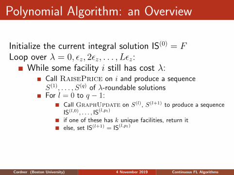
Initialize the current integral solution IS(0) = F
Loop over λ = 0, εz, 2εz, . . . , Lεz:While some facility i still has cost λ:
Call RaisePrice on i and produce a sequenceS(1), . . . , S(q) of λ-roundable solutionsFor l = 0 to q − 1:
Call GraphUpdate on S(l), S(l+1) to produce a sequenceIS(l,0), . . . , IS(l,pl)
if one of these has k unique facilities, return itelse, set IS(l+1) = IS(l,pl)
Reset S(0) = S(q), IS(0) = IS(q)
Cordner (Boston University) 4 November 2019 Continuous FL Algorithms

Polynomial Algorithm: an Overview
Initialize the current integral solution IS(0) = FLoop over λ = 0, εz, 2εz, . . . , Lεz:
While some facility i still has cost λ:Call RaisePrice on i and produce a sequenceS(1), . . . , S(q) of λ-roundable solutionsFor l = 0 to q − 1:
Call GraphUpdate on S(l), S(l+1) to produce a sequenceIS(l,0), . . . , IS(l,pl)
if one of these has k unique facilities, return itelse, set IS(l+1) = IS(l,pl)
Reset S(0) = S(q), IS(0) = IS(q)
Cordner (Boston University) 4 November 2019 Continuous FL Algorithms

Polynomial Algorithm: an Overview
Initialize the current integral solution IS(0) = FLoop over λ = 0, εz, 2εz, . . . , Lεz:
While some facility i still has cost λ:
Call RaisePrice on i and produce a sequenceS(1), . . . , S(q) of λ-roundable solutionsFor l = 0 to q − 1:
Call GraphUpdate on S(l), S(l+1) to produce a sequenceIS(l,0), . . . , IS(l,pl)
if one of these has k unique facilities, return itelse, set IS(l+1) = IS(l,pl)
Reset S(0) = S(q), IS(0) = IS(q)
Cordner (Boston University) 4 November 2019 Continuous FL Algorithms

Polynomial Algorithm: an Overview
Initialize the current integral solution IS(0) = FLoop over λ = 0, εz, 2εz, . . . , Lεz:
While some facility i still has cost λ:Call RaisePrice on i and produce a sequenceS(1), . . . , S(q) of λ-roundable solutions
For l = 0 to q − 1:Call GraphUpdate on S(l), S(l+1) to produce a sequenceIS(l,0), . . . , IS(l,pl)
if one of these has k unique facilities, return itelse, set IS(l+1) = IS(l,pl)
Reset S(0) = S(q), IS(0) = IS(q)
Cordner (Boston University) 4 November 2019 Continuous FL Algorithms

Polynomial Algorithm: an Overview
Initialize the current integral solution IS(0) = FLoop over λ = 0, εz, 2εz, . . . , Lεz:
While some facility i still has cost λ:Call RaisePrice on i and produce a sequenceS(1), . . . , S(q) of λ-roundable solutionsFor l = 0 to q − 1:
Call GraphUpdate on S(l), S(l+1) to produce a sequenceIS(l,0), . . . , IS(l,pl)
if one of these has k unique facilities, return itelse, set IS(l+1) = IS(l,pl)
Reset S(0) = S(q), IS(0) = IS(q)
Cordner (Boston University) 4 November 2019 Continuous FL Algorithms

Polynomial Algorithm: an Overview
Initialize the current integral solution IS(0) = FLoop over λ = 0, εz, 2εz, . . . , Lεz:
While some facility i still has cost λ:Call RaisePrice on i and produce a sequenceS(1), . . . , S(q) of λ-roundable solutionsFor l = 0 to q − 1:
Call GraphUpdate on S(l), S(l+1) to produce a sequenceIS(l,0), . . . , IS(l,pl)
if one of these has k unique facilities, return it
else, set IS(l+1) = IS(l,pl)
Reset S(0) = S(q), IS(0) = IS(q)
Cordner (Boston University) 4 November 2019 Continuous FL Algorithms
Polynomial Algorithm: an Overview
Initialize the current integral solution IS(0) = FLoop over λ = 0, εz, 2εz, . . . , Lεz:
While some facility i still has cost λ:Call RaisePrice on i and produce a sequenceS(1), . . . , S(q) of λ-roundable solutionsFor l = 0 to q − 1:
Call GraphUpdate on S(l), S(l+1) to produce a sequenceIS(l,0), . . . , IS(l,pl)
if one of these has k unique facilities, return itelse, set IS(l+1) = IS(l,pl)
Reset S(0) = S(q), IS(0) = IS(q)
Cordner (Boston University) 4 November 2019 Continuous FL Algorithms

Polynomial Algorithm: an Overview
Initialize the current integral solution IS(0) = FLoop over λ = 0, εz, 2εz, . . . , Lεz:
While some facility i still has cost λ:Call RaisePrice on i and produce a sequenceS(1), . . . , S(q) of λ-roundable solutionsFor l = 0 to q − 1:
Call GraphUpdate on S(l), S(l+1) to produce a sequenceIS(l,0), . . . , IS(l,pl)
if one of these has k unique facilities, return itelse, set IS(l+1) = IS(l,pl)
Reset S(0) = S(q), IS(0) = IS(q)
Cordner (Boston University) 4 November 2019 Continuous FL Algorithms

Polynomial Algorithm: an Overview
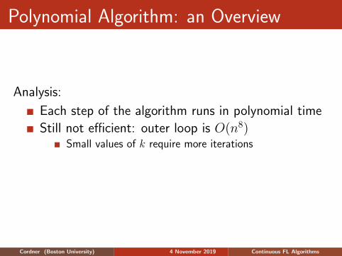
Analysis:
Each step of the algorithm runs in polynomial time
Still not efficient: outer loop is O(n8)Small values of k require more iterations
Returned solution is a (ρ+O(ε))-approximation
Cordner (Boston University) 4 November 2019 Continuous FL Algorithms

Polynomial Algorithm: an Overview
Analysis:
Each step of the algorithm runs in polynomial time
Still not efficient: outer loop is O(n8)Small values of k require more iterations
Returned solution is a (ρ+O(ε))-approximation
Cordner (Boston University) 4 November 2019 Continuous FL Algorithms

Polynomial Algorithm: an Overview
Analysis:
Each step of the algorithm runs in polynomial time
Still not efficient: outer loop is O(n8)
Small values of k require more iterations
Returned solution is a (ρ+O(ε))-approximation
Cordner (Boston University) 4 November 2019 Continuous FL Algorithms
Polynomial Algorithm: an Overview
Analysis:
Each step of the algorithm runs in polynomial time
Still not efficient: outer loop is O(n8)Small values of k require more iterations
Returned solution is a (ρ+O(ε))-approximation
Cordner (Boston University) 4 November 2019 Continuous FL Algorithms

Polynomial Algorithm: an Overview
Analysis:
Each step of the algorithm runs in polynomial time
Still not efficient: outer loop is O(n8)Small values of k require more iterations
Returned solution is a (ρ+O(ε))-approximation
Cordner (Boston University) 4 November 2019 Continuous FL Algorithms

In Summary
We discussed the JV facility location algorithm
Good approximations to k-means and k-medianwhen it opens k facilities
We overviewed three modifications to make the JValgorithm continuous
Guaranteed to find k facilities for any value of k
Can we do the same for other LMP algorithms?
Cordner (Boston University) 4 November 2019 Continuous FL Algorithms

Cordner (Boston University) 4 November 2019 Continuous FL Algorithms