Embed Size (px)
Citation preview
1
2
3
4
5
6
7
8
9
10
11
12
13
14
15
16
17
18
19
20
21
22
23
24
25
26
27
28
29
30
31
32
33
34
35
36
37
38
39
40
41
42
43
44
45
46
47
48
49
1
Contextual Equivalence for a Probabilistic Language withContinuous Random Variables and Recursion
MITCHELL WAND, Northeastern University
RYAN CULPEPPER, Northeastern University
THEOPHILOS GIANNAKOPOULOS, BAE Systems, Burlington MA
ANDREW COBB, Northeastern University
We present a complete reasoning principle for contextual equivalence in an untyped probabilistic language.
The language includes continuous (real-valued) random variables, conditionals, and scoring. It also includes
recursion, since the standard call-by-value fixpoint combinator is expressible.
We demonstrate the usability of our characterization by proving several equivalence schemas, including
familiar facts from lambda calculus as well as results specific to probabilistic programming. In particular, we
use it to prove that reordering the random draws in a probabilistic program preserves contextual equivalence.
This allows us to show, for example, that
(letx = e1 in lety = e2 in e0) =ctx (lety = e2 in letx = e1 in e0)
(provided x does not occur free in e2 and y does not occur free in e1) despite the fact that e1 and e2 may have
sampling and scoring effects.
CCS Concepts: • Mathematics of computing → Probability and statistics; • Theory of computation→ Operational semantics;
Additional Key Words and Phrases: probabilistic programming, logical relations, contextual equivalence
ACM Reference format:Mitchell Wand, Ryan Culpepper, Theophilos Giannakopoulos, and Andrew Cobb. 2017. Contextual Equivalence
for a Probabilistic Language with Continuous Random Variables and Recursion. Proc. ACM Program. Lang. 1,1, Article 1 (January 2017), 35 pages.
https://doi.org/10.1145/nnnnnnn.nnnnnnn
1 INTRODUCTIONA probabilistic programming language is a programming language enriched with two features—
sampling and scoring—that enable it to represent probabilistic models. We introduce these two
features with an example program that models linear regression.
The first feature, sampling, introduces probabilistic nondeterminism. It is used to represent
random variables. For example, let normal(m, s) be defined to nondeterministically produce a real
number distributed according to a normal (Gaussian) distribution with meanm and scale s .Here is a little model of linear regression that uses normal to randomly pick a slope and intercept
for a line and then defines f as the resulting linear function:
A = normal(0, 10)B = normal(0, 10)f(x) = A*x + B
This material is based upon work sponsored by the Air Force Research Laboratory (AFRL) and the Defense Advanced
Research Projects Agency (DARPA) under Contract No. FA8750-14-C-0002. The views expressed are those of the authors
and do not reflect the official policy or position of the Department of Defense or the U.S. Government.
2017. 2475-1421/2017/1-ART1 $15.00
https://doi.org/10.1145/nnnnnnn.nnnnnnn
Proc. ACM Program. Lang., Vol. 1, No. 1, Article 1. Publication date: January 2017.

50
51
52
53
54
55
56
57
58
59
60
61
62
63
64
65
66
67
68
69
70
71
72
73
74
75
76
77
78
79
80
81
82
83
84
85
86
87
88
89
90
91
92
93
94
95
96
97
98
1:2 Mitchell Wand, Ryan Culpepper, Theophilos Giannakopoulos, and Andrew Cobb
This program defines a distribution on lines, centered on y = 0x + 0, with high variance. This
distribution is called the prior, since it is specified prior to considering any evidence.
The second feature, scoring, adjusts the likelihood of the current execution’s random choices. It
is used to represent conditioning on observed data.
Suppose we have the following data points: (2.0, 2.4), (3.0, 2.7), (4.0, 3.0). The smaller the error
between the result of f and the observed data, the better the choice of A and B. We express these
observations with the following addition to our program:
factor normalpdf(f(2.0)-2.4; 0, 1)factor normalpdf(f(3.0)-2.7; 0, 1)factor normalpdf(f(4.0)-3.0; 0, 1)
Here scoring is performed by the factor form, which takes a positive real number to multiply
into the current execution’s likelihood. We use normalpdf(_; 0,1)—the density function of the
standard normal distribution—to convert the difference between predicted and observed values
into the score. This scoring function assigns high likelihood when the error is near 0, dropping off
smoothly to low likelihood for larger errors.
After incorporating the observations, the program defines a distribution centered near y =0.3x + 1.8, with low variance. This distribution is often called the posterior distribution, since itrepresents the distribution after the incorporation of evidence.
Computing the posterior distribution—or a workable approximation thereof—is the task of proba-bilistic inference. We say that this program has inferred (or sometimes learned) the parameters A andB from the data. Probabilistic inference encompasses an arsenal of techniques of varied applicability
and efficiency. Some inference techniques may benefit if the program above is transformed to the
following shape:
A = normal(0, 10)factor Z(A)B = normal(M(A), S(A))
The transformation relies on the conjugacy relationship between the normal prior for B and
the normal scoring function of the observations. A useful equational theory for probabilistic
programming must incorporate facts from mathematics in addition to standard concerns such as
function inlining.
In this paper we build a foundation for such an equational theory for a probabilistic programming
language. In particular, our language supports
• sampling continuous random variables,
• scoring (soft constraints), and
• conditionals, higher-order functions, and recursion.
Other such languages include Church [?], its descendants such as Venture [?] and Anglican [?], andother languages [???] and languagemodels [???]. Our framework is able to justify the transformation
above.
In Section 2 we present our model of a probabilistic language, including its syntax and semantics.
We then define our logical relation (Section 3), our CIU relation (Section 4), and contextual ordering
(Section 5); and we prove that all three relations coincide. In Section 6 we use this new machinery to
define contextual equivalence and demonstrate a catalog of useful equivalence schemas, including βvand let-associativity, as well as a method for importing first-order equivalences from mathematics.
One unusual equivalence is let-commutativity:
(letx = e1 in lety = e2 in e0) =ctx (lety = e2 in letx = e1 in e0)
Proc. ACM Program. Lang., Vol. 1, No. 1, Article 1. Publication date: January 2017.
99
100
101
102
103
104
105
106
107
108
109
110
111
112
113
114
115
116
117
118
119
120
121
122
123
124
125
126
127
128
129
130
131
132
133
134
135
136
137
138
139
140
141
142
143
144
145
146
147
Contextual Equivalence for a Probabilistic Language with Continuous Random Variables andRecursion 1:3
(provided x does not occur free in e2 and y does not occur free in e1). This equivalence, whilevalid for a pure language, is certainly not valid for all effects (consider, for example, if there were
an assignment statement in e1 or e2). We conclude with two related work sections: Section 7
demonstrates the correspondence between our language model and others, notably that of ?, andSection 8 informally discusses other related work.
Throughout the paper, we limit proofs mostly to high-level sketches and representative cases.
Additional details and cases for some proofs can be found in Appendix A.
Appendix B sketches the steps of the linear regression transformation above using the equiva-
lences we prove in this paper.
2 PROBABILISTIC LANGUAGE MODELIn this section we define our probabilistic language and its semantics. The semantics consists of
three parts:
• A notion of entropy for modeling random behavior.
• An evaluation function that maps a program and entropy to a real-valued result and an
importance weight. We define the evaluation function via an abstract machine. We then
define a big-step semantics and prove it equivalent; the big-step formulation simplifies some
proofs in Section 6.3 by making the structure of evaluation explicit.
• A mapping to measures over the real numbers, calculated by integrating the evaluation
function with respect to the entropy space. A program with a finite, non-zero measure can
be interpreted as an unnormalized probability distribution.
The structure of the semantics loosely corresponds to one inference technique for probabilistic
programming languages: importance sampling. In an importance sampler, the entropy is approxi-
mated by a pseudo-random number generator (PRNG); the evaluation function is run many times
with different initial PRNG states to produce a collection of weighted samples; and the weighted
samples approximate the program’s measure—either directly by conversion to a discrete distribution
of results, or indirectly via computed statistical properties such as sample mean, variance, etc.
Our language is similar to that of ?, but with the following differences:
• Our language requires let-binding of nontrivial intermediate expressions; this simplifies the
semantics. This restriction is similar to but looser than A-normal form [?].• Our model of entropy is a finite measure space made of splittable entropy points, rather than
an infinite measure space containing sequences of real numbers.
• Our sample operation models a standard uniform random variable, rather than being param-
eterized over a distribution.
We revisit these differences in Section 7.
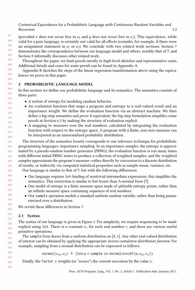
2.1 SyntaxThe syntax of our language is given in Figure 1. For simplicity, we require sequencing to be made
explicit using let. There is a constant cr for each real number r , and there are various useful
primitive operations.
The sample form draws from a uniform distribution on [0, 1]. Any other real-valued distribution
of interest can be obtained by applying the appropriate inverse cumulative distribution function. Forexample, sampling from a normal distribution can be expressed as follows:
normal(vm ,vs) ≜ (letu = sample in normalinvcdf(u;vm ,vs))
Finally, the factor v weights (or “scores”) the current execution by the value v .
Proc. ACM Program. Lang., Vol. 1, No. 1, Article 1. Publication date: January 2017.
148
149
150
151
152
153
154
155
156
157
158
159
160
161
162
163
164
165
166
167
168
169
170
171
172
173
174
175
176
177
178
179
180
181
182
183
184
185
186
187
188
189
190
191
192
193
194
195
196
1:4 Mitchell Wand, Ryan Culpepper, Theophilos Giannakopoulos, and Andrew Cobb
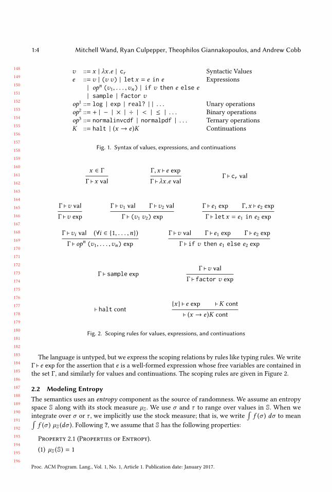
v ::= x | λx .e | cr Syntactic Values
e ::= v | (v v) | letx = e in e Expressions
| opn (v1, . . . ,vn) | if v then e else e| sample | factor v
op1 ::= log | exp | real? | | . . . Unary operations
op2 ::= + | − | × | ÷ | < | ≤ | . . . Binary operations
op3 ::= normalinvcdf | normalpdf | . . . Ternary operations
K ::= halt | (x → e )K Continuations
Fig. 1. Syntax of values, expressions, and continuations
x ∈ Γ
Γ ⊢x val
Γ,x ⊢ e exp
Γ ⊢ λx .e valΓ ⊢ cr val
Γ ⊢v val
Γ ⊢v exp
Γ ⊢v1 val Γ ⊢v2 val
Γ ⊢ (v1 v2) exp
Γ ⊢ e1 exp Γ,x ⊢ e2 exp
Γ ⊢ letx = e1 in e2 exp
Γ ⊢vi val (∀i ∈ 1, . . . ,n)
Γ ⊢ opn (v1, . . . ,vn) exp
Γ ⊢v val Γ ⊢ e1 exp Γ ⊢ e2 exp
Γ ⊢ if v then e1 else e2 exp
Γ ⊢ sample expΓ ⊢v val
Γ ⊢ factor v exp
⊢ halt contx ⊢ e exp ⊢K cont
⊢ (x → e )K cont
Fig. 2. Scoping rules for values, expressions, and continuations
The language is untyped, but we express the scoping relations by rules like typing rules. We write
Γ ⊢ e exp for the assertion that e is a well-formed expression whose free variables are contained in
the set Γ, and similarly for values and continuations. The scoping rules are given in Figure 2.
2.2 Modeling EntropyThe semantics uses an entropy component as the source of randomness. We assume an entropy
space S along with its stock measure µS. We use σ and τ to range over values in S. When we
integrate over σ or τ , we implicitly use the stock measure; that is, we write
∫f (σ ) dσ to mean∫
f (σ ) µS (dσ ). Following ?, we assume that S has the following properties:
Property 2.1 (Properties of Entropy).
(1) µS (S) = 1
Proc. ACM Program. Lang., Vol. 1, No. 1, Article 1. Publication date: January 2017.
197
198
199
200
201
202
203
204
205
206
207
208
209
210
211
212
213
214
215
216
217
218
219
220
221
222
223
224
225
226
227
228
229
230
231
232
233
234
235
236
237
238
239
240
241
242
243
244
245
Contextual Equivalence for a Probabilistic Language with Continuous Random Variables andRecursion 1:5
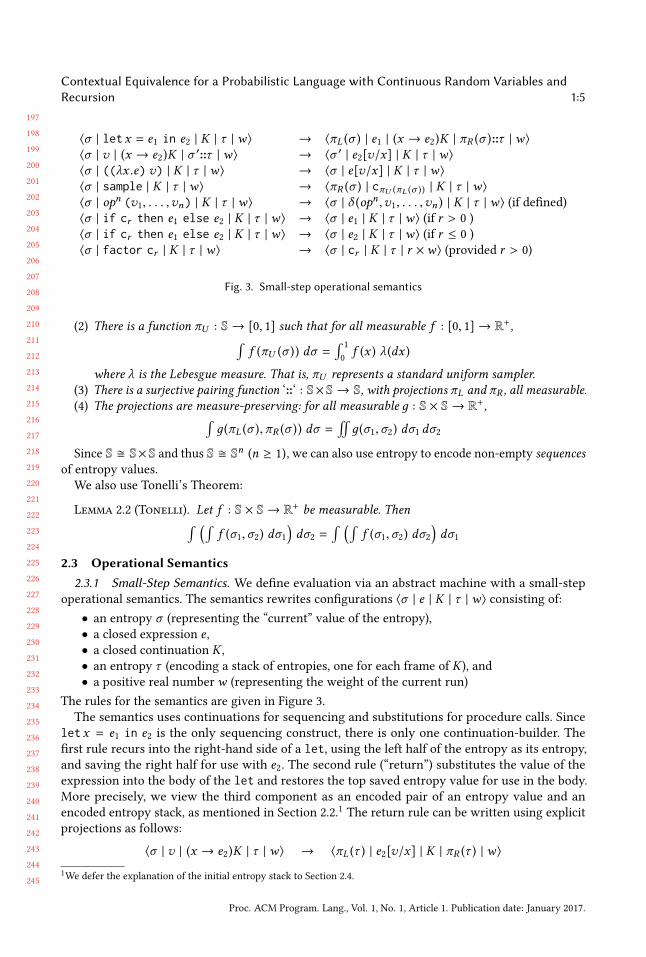
⟨σ | letx = e1 in e2 | K | τ | w⟩ → ⟨πL (σ ) | e1 | (x → e2)K | πR (σ )::τ | w⟩⟨σ | v | (x → e2)K | σ
′::τ | w⟩ → ⟨σ ′ | e2[v/x] | K | τ | w⟩⟨σ | ((λx .e) v) | K | τ | w⟩ → ⟨σ | e[v/x] | K | τ | w⟩⟨σ | sample | K | τ | w⟩ → ⟨πR (σ ) | cπU (πL (σ )) | K | τ | w⟩⟨σ | opn (v1, . . . ,vn) | K | τ | w⟩ → ⟨σ | δ (opn ,v1, . . . ,vn ) | K | τ | w⟩ (if defined)⟨σ | if cr then e1 else e2 | K | τ | w⟩ → ⟨σ | e1 | K | τ | w⟩ (if r > 0 )
⟨σ | if cr then e1 else e2 | K | τ | w⟩ → ⟨σ | e2 | K | τ | w⟩ (if r ≤ 0 )
⟨σ | factor cr | K | τ | w⟩ → ⟨σ | cr | K | τ | r ×w⟩ (provided r > 0)
Fig. 3. Small-step operational semantics
(2) There is a function πU : S→ [0, 1] such that for all measurable f : [0, 1]→ R+,∫f (πU (σ )) dσ =
∫1
0f (x ) λ(dx )
where λ is the Lebesgue measure. That is, πU represents a standard uniform sampler.(3) There is a surjective pairing function ‘::‘ : S×S→ S, with projections πL and πR , all measurable.(4) The projections are measure-preserving: for all measurable д : S × S→ R+,∫
д(πL (σ ),πR (σ )) dσ =!
д(σ1,σ2) dσ1 dσ2
Since S S×S and thus S Sn (n ≥ 1), we can also use entropy to encode non-empty sequencesof entropy values.
We also use Tonelli’s Theorem:
Lemma 2.2 (Tonelli). Let f : S × S→ R+ be measurable. Then∫ (∫f (σ1,σ2) dσ1
)dσ2 =
∫ (∫f (σ1,σ2) dσ2
)dσ1
2.3 Operational Semantics2.3.1 Small-Step Semantics. We define evaluation via an abstract machine with a small-step
operational semantics. The semantics rewrites configurations ⟨σ | e | K | τ | w⟩ consisting of:
• an entropy σ (representing the “current” value of the entropy),
• a closed expression e ,• a closed continuation K ,• an entropy τ (encoding a stack of entropies, one for each frame of K ), and• a positive real numberw (representing the weight of the current run)
The rules for the semantics are given in Figure 3.
The semantics uses continuations for sequencing and substitutions for procedure calls. Since
letx = e1 in e2 is the only sequencing construct, there is only one continuation-builder. The
first rule recurs into the right-hand side of a let, using the left half of the entropy as its entropy,
and saving the right half for use with e2. The second rule (“return”) substitutes the value of the
expression into the body of the let and restores the top saved entropy value for use in the body.
More precisely, we view the third component as an encoded pair of an entropy value and an
encoded entropy stack, as mentioned in Section 2.2.1The return rule can be written using explicit
projections as follows:
⟨σ | v | (x → e2)K | τ | w⟩ → ⟨πL (τ ) | e2[v/x] | K | πR (τ ) | w⟩
1We defer the explanation of the initial entropy stack to Section 2.4.
Proc. ACM Program. Lang., Vol. 1, No. 1, Article 1. Publication date: January 2017.
246
247
248
249
250
251
252
253
254
255
256
257
258
259
260
261
262
263
264
265
266
267
268
269
270
271
272
273
274
275
276
277
278
279
280
281
282
283
284
285
286
287
288
289
290
291
292
293
294
1:6 Mitchell Wand, Ryan Culpepper, Theophilos Giannakopoulos, and Andrew Cobb
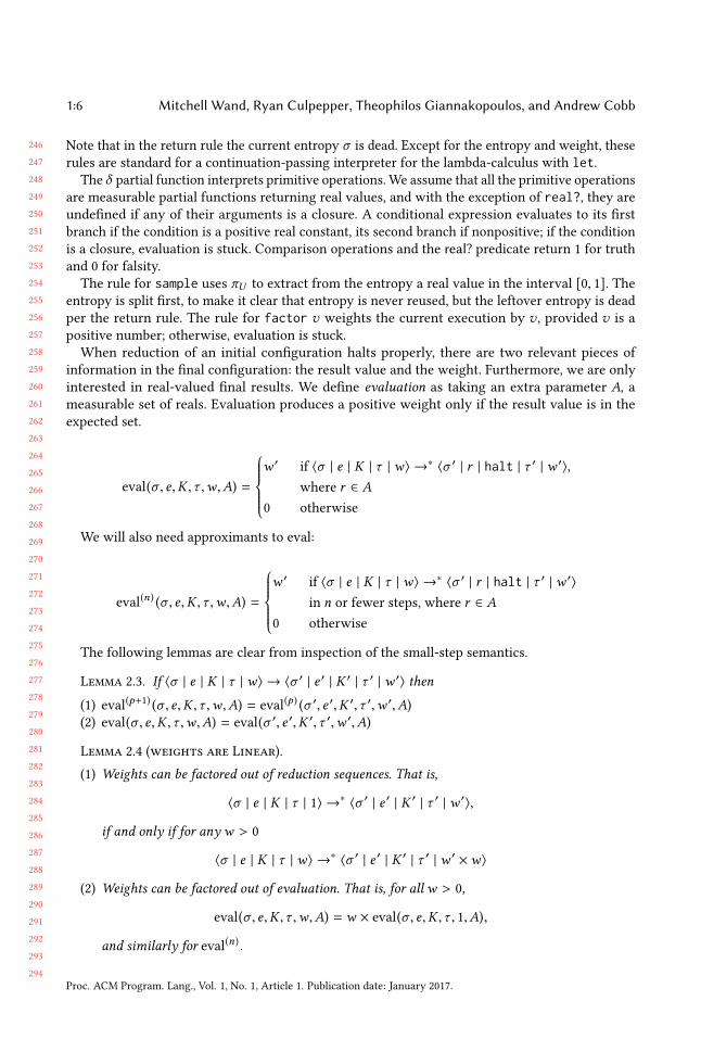
Note that in the return rule the current entropy σ is dead. Except for the entropy and weight, these
rules are standard for a continuation-passing interpreter for the lambda-calculus with let.The δ partial function interprets primitive operations. We assume that all the primitive operations
are measurable partial functions returning real values, and with the exception of real?, they are
undefined if any of their arguments is a closure. A conditional expression evaluates to its first
branch if the condition is a positive real constant, its second branch if nonpositive; if the condition
is a closure, evaluation is stuck. Comparison operations and the real? predicate return 1 for truth
and 0 for falsity.
The rule for sample uses πU to extract from the entropy a real value in the interval [0, 1]. Theentropy is split first, to make it clear that entropy is never reused, but the leftover entropy is dead
per the return rule. The rule for factor v weights the current execution by v , provided v is a
positive number; otherwise, evaluation is stuck.
When reduction of an initial configuration halts properly, there are two relevant pieces of
information in the final configuration: the result value and the weight. Furthermore, we are only
interested in real-valued final results. We define evaluation as taking an extra parameter A, ameasurable set of reals. Evaluation produces a positive weight only if the result value is in the
expected set.
eval(σ , e,K ,τ ,w,A) =
w ′ if ⟨σ | e | K | τ | w⟩ →∗ ⟨σ ′ | r | halt | τ ′ | w ′⟩,
where r ∈ A
0 otherwise
We will also need approximants to eval:
eval(n) (σ , e,K ,τ ,w,A) =
w ′ if ⟨σ | e | K | τ | w⟩ →∗ ⟨σ ′ | r | halt | τ ′ | w ′⟩
in n or fewer steps, where r ∈ A
0 otherwise
The following lemmas are clear from inspection of the small-step semantics.
Lemma 2.3. If ⟨σ | e | K | τ | w⟩ → ⟨σ ′ | e ′ | K ′ | τ ′ | w ′⟩ then
(1) eval(p+1) (σ , e,K ,τ ,w,A) = eval
(p ) (σ ′, e ′,K ′,τ ′,w ′,A)(2) eval(σ , e,K ,τ ,w,A) = eval(σ ′, e ′,K ′,τ ′,w ′,A)
Lemma 2.4 (weights are Linear).
(1) Weights can be factored out of reduction sequences. That is,
⟨σ | e | K | τ | 1⟩ →∗ ⟨σ ′ | e ′ | K ′ | τ ′ | w ′⟩,
if and only if for anyw > 0
⟨σ | e | K | τ | w⟩ →∗ ⟨σ ′ | e ′ | K ′ | τ ′ | w ′ ×w⟩
(2) Weights can be factored out of evaluation. That is, for allw > 0,
eval(σ , e,K ,τ ,w,A) = w × eval(σ , e,K ,τ , 1,A),
and similarly for eval(n) .
Proc. ACM Program. Lang., Vol. 1, No. 1, Article 1. Publication date: January 2017.
295
296
297
298
299
300
301
302
303
304
305
306
307
308
309
310
311
312
313
314
315
316
317
318
319
320
321
322
323
324
325
326
327
328
329
330
331
332
333
334
335
336
337
338
339
340
341
342
343
Contextual Equivalence for a Probabilistic Language with Continuous Random Variables andRecursion 1:7
σ ⊢ λx .e ⇓ λx .e, 1 σ ⊢ cr ⇓ cr , 1
σ ⊢ e[v/x] ⇓ v ′,w
σ ⊢ ((λx .e) v) ⇓ v ′,w
πL (σ ) ⊢ e1 ⇓ v1,w1 πR (σ ) ⊢ e2[v1/x] ⇓ v2,w2
σ ⊢ letx = e1 in e2 ⇓ v2,w2 ×w1
δ (opn ,v1, . . . ,vn ) = v
σ ⊢ opn (v1, . . . ,vn) ⇓ v, 1
σ ⊢ e1 ⇓ v,w r > 0
σ ⊢ if cr then e1 else e2 ⇓ v,w
σ ⊢ e2 ⇓ v,w r ≤ 0
σ ⊢ if cr then e1 else e2 ⇓ v,w
σ ⊢ sample ⇓ cπU (πL (σ )), 1r > 0
σ ⊢ factor cr ⇓ cr , r
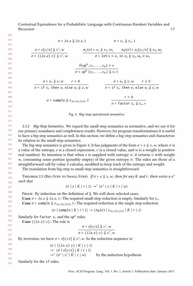
Fig. 4. Big-step operational semantics
2.3.2 Big-Step Semantics. We regard the small-step semantics as normative, and we use it for
our primary soundness and completeness results. However, for program transformations it is useful
to have a big-step semantics as well. In this section, we define a big-step semantics and characterize
its relation to the small-step semantics.
The big-step semantics is given in Figure 4. It has judgments of the form σ ⊢ e ⇓ v,w , where σ is
a value of the entropy, e is a closed expression, v is a closed value, and w is a weight (a positive
real number). Its intention is that when e is supplied with entropy σ , it returns v with weight
w , consuming some portion (possibly empty) of the given entropy σ . The rules are those of a
straightforward call-by-value λ-calculus, modified to keep track of the entropy and weight.
The translation from big-step to small-step semantics is straightforward:
Theorem 2.5 (Big-Step to Small-Step). If σ ⊢ e ⇓ v,w , then for any K and τ , there exists a σ ′
such that⟨σ | e | K | τ | 1⟩ →∗ ⟨σ ′ | v | K | τ | w⟩
Proof. By induction on the definition of ⇓. We will show selected cases.
Case σ ⊢ λx .e ⇓ λx .e, 1 : The required small-step reduction is empty. Similarly for cr .Case σ ⊢ sample ⇓ cπU (πL (σ )), 1 : The required reduction is the single step reduction
⟨σ | sample | K | τ | 1⟩ → ⟨πR (σ ) | cπU (πL (σ )) | K | τ | 1⟩
Similarly for factor cr and the opn rules.
Case ((λx .e) v) : The rule isσ ⊢ e[v/x] ⇓ v ′,w
σ ⊢ ((λx .e) v) ⇓ v ′,w
By inversion, we have σ ⊢ e[v/x] ⇓ v ′,w . So the reduction sequence is:
⟨σ | ((λx .e) v) | K | τ | 1⟩→ ⟨σ | e[v/x] | K | τ | 1⟩→∗ ⟨σ ′ | v ′ | K | τ | w⟩ by the induction hypothesis
Similarly for the if rules.
Proc. ACM Program. Lang., Vol. 1, No. 1, Article 1. Publication date: January 2017.
344
345
346
347
348
349
350
351
352
353
354
355
356
357
358
359
360
361
362
363
364
365
366
367
368
369
370
371
372
373
374
375
376
377
378
379
380
381
382
383
384
385
386
387
388
389
390
391
392
1:8 Mitchell Wand, Ryan Culpepper, Theophilos Giannakopoulos, and Andrew Cobb
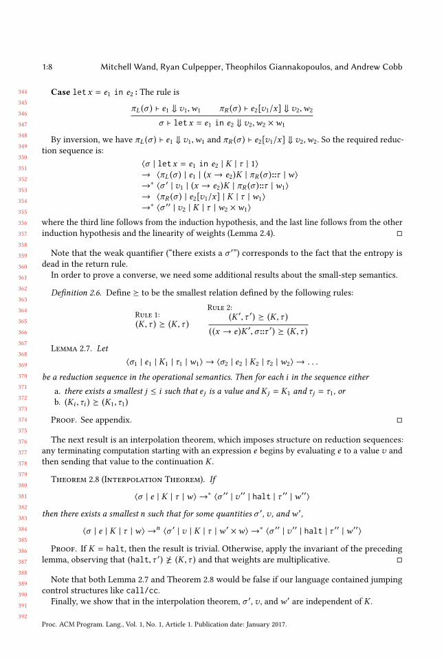
Case letx = e1 in e2 : The rule is
πL (σ ) ⊢ e1 ⇓ v1,w1 πR (σ ) ⊢ e2[v1/x] ⇓ v2,w2
σ ⊢ letx = e1 in e2 ⇓ v2,w2 ×w1
By inversion, we have πL (σ ) ⊢ e1 ⇓ v1,w1 and πR (σ ) ⊢ e2[v1/x] ⇓ v2,w2. So the required reduc-
tion sequence is:
⟨σ | letx = e1 in e2 | K | τ | 1⟩→ ⟨πL (σ ) | e1 | (x → e2)K | πR (σ )::τ | w⟩→∗ ⟨σ ′ | v1 | (x → e2)K | πR (σ )::τ | w1⟩
→ ⟨πR (σ ) | e2[v1/x] | K | τ | w1⟩
→∗ ⟨σ ′′ | v2 | K | τ | w2 ×w1⟩
where the third line follows from the induction hypothesis, and the last line follows from the other
induction hypothesis and the linearity of weights (Lemma 2.4).
Note that the weak quantifier (“there exists a σ ′”) corresponds to the fact that the entropy is
dead in the return rule.
In order to prove a converse, we need some additional results about the small-step semantics.
Definition 2.6. Define ⪰ to be the smallest relation defined by the following rules:
Rule 1:
(K ,τ ) ⪰ (K ,τ )
Rule 2:
(K ′,τ ′) ⪰ (K ,τ )
((x → e )K ′,σ ::τ ′) ⪰ (K ,τ )
Lemma 2.7. Let⟨σ1 | e1 | K1 | τ1 | w1⟩ → ⟨σ2 | e2 | K2 | τ2 | w2⟩ → . . .
be a reduction sequence in the operational semantics. Then for each i in the sequence either
a. there exists a smallest j ≤ i such that ej is a value and Kj = K1 and τj = τ1, orb. (Ki ,τi ) ⪰ (K1,τ1)
Proof. See appendix.
The next result is an interpolation theorem, which imposes structure on reduction sequences:
any terminating computation starting with an expression e begins by evaluating e to a value v and
then sending that value to the continuation K .
Theorem 2.8 (Interpolation Theorem). If
⟨σ | e | K | τ | w⟩ →∗ ⟨σ ′′ | v ′′ | halt | τ ′′ | w ′′⟩
then there exists a smallest n such that for some quantities σ ′, v , andw ′,
⟨σ | e | K | τ | w⟩ →n ⟨σ ′ | v | K | τ | w ′ ×w⟩ →∗ ⟨σ ′′ | v ′′ | halt | τ ′′ | w ′′⟩
Proof. If K = halt, then the result is trivial. Otherwise, apply the invariant of the preceding
lemma, observing that (halt,τ ′) ⪰ (K ,τ ) and that weights are multiplicative.
Note that both Lemma 2.7 and Theorem 2.8 would be false if our language contained jumping
control structures like call/cc.Finally, we show that in the interpolation theorem, σ ′, v , andw ′ are independent of K .
Proc. ACM Program. Lang., Vol. 1, No. 1, Article 1. Publication date: January 2017.
393
394
395
396
397
398
399
400
401
402
403
404
405
406
407
408
409
410
411
412
413
414
415
416
417
418
419
420
421
422
423
424
425
426
427
428
429
430
431
432
433
434
435
436
437
438
439
440
441
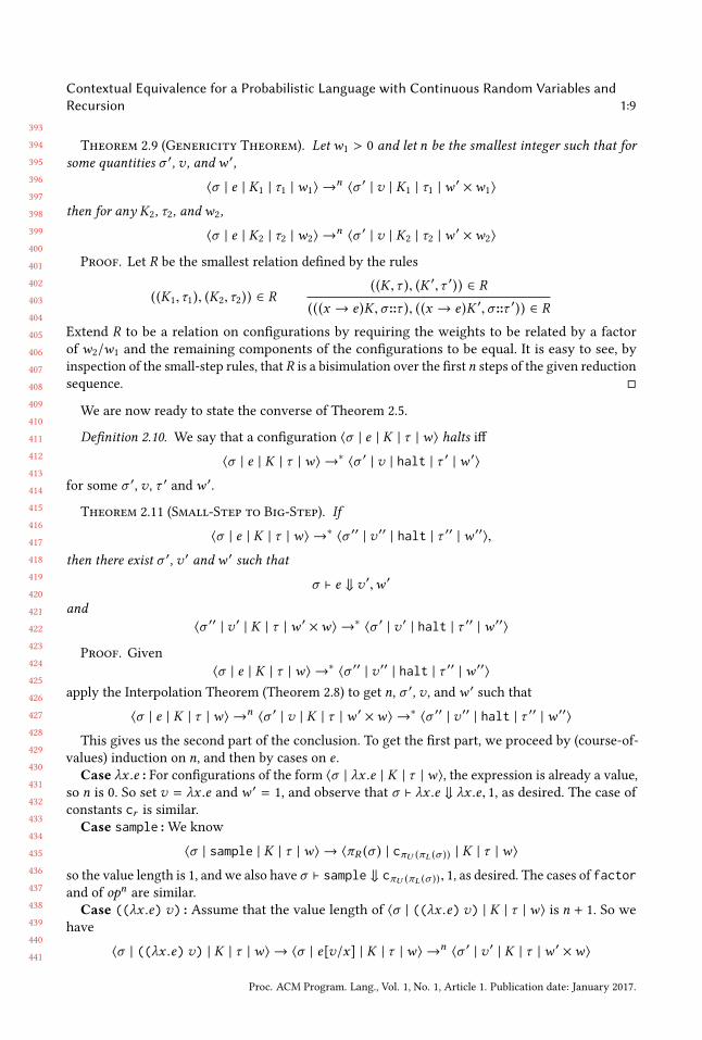
Contextual Equivalence for a Probabilistic Language with Continuous Random Variables andRecursion 1:9
Theorem 2.9 (Genericity Theorem). Letw1 > 0 and let n be the smallest integer such that forsome quantities σ ′, v , andw ′,
⟨σ | e | K1 | τ1 | w1⟩ →n ⟨σ ′ | v | K1 | τ1 | w
′ ×w1⟩
then for any K2, τ2, andw2,
⟨σ | e | K2 | τ2 | w2⟩ →n ⟨σ ′ | v | K2 | τ2 | w
′ ×w2⟩
Proof. Let R be the smallest relation defined by the rules
((K1,τ1), (K2,τ2)) ∈ R((K ,τ ), (K ′,τ ′)) ∈ R
(((x → e )K ,σ ::τ ), ((x → e )K ′,σ ::τ ′)) ∈ R
Extend R to be a relation on configurations by requiring the weights to be related by a factor
of w2/w1 and the remaining components of the configurations to be equal. It is easy to see, by
inspection of the small-step rules, that R is a bisimulation over the first n steps of the given reduction
sequence.
We are now ready to state the converse of Theorem 2.5.
Definition 2.10. We say that a configuration ⟨σ | e | K | τ | w⟩ halts iff
⟨σ | e | K | τ | w⟩ →∗ ⟨σ ′ | v | halt | τ ′ | w ′⟩
for some σ ′, v , τ ′ andw ′.
Theorem 2.11 (Small-Step to Big-Step). If
⟨σ | e | K | τ | w⟩ →∗ ⟨σ ′′ | v ′′ | halt | τ ′′ | w ′′⟩,
then there exist σ ′, v ′ andw ′ such that
σ ⊢ e ⇓ v ′,w ′
and⟨σ ′′ | v ′ | K | τ | w ′ ×w⟩ →∗ ⟨σ ′ | v ′ | halt | τ ′′ | w ′′⟩
Proof. Given
⟨σ | e | K | τ | w⟩ →∗ ⟨σ ′′ | v ′′ | halt | τ ′′ | w ′′⟩
apply the Interpolation Theorem (Theorem 2.8) to get n, σ ′, v , andw ′ such that
⟨σ | e | K | τ | w⟩ →n ⟨σ ′ | v | K | τ | w ′ ×w⟩ →∗ ⟨σ ′′ | v ′′ | halt | τ ′′ | w ′′⟩
This gives us the second part of the conclusion. To get the first part, we proceed by (course-of-
values) induction on n, and then by cases on e .Case λx .e : For configurations of the form ⟨σ | λx .e | K | τ | w⟩, the expression is already a value,
so n is 0. So set v = λx .e and w ′ = 1, and observe that σ ⊢ λx .e ⇓ λx .e, 1, as desired. The case ofconstants cr is similar.
Case sample :We know
⟨σ | sample | K | τ | w⟩ → ⟨πR (σ ) | cπU (πL (σ )) | K | τ | w⟩
so the value length is 1, and we also have σ ⊢ sample ⇓ cπU (πL (σ )), 1, as desired. The cases of factorand of opn are similar.
Case ((λx .e) v) : Assume that the value length of ⟨σ | ((λx .e) v) | K | τ | w⟩ is n + 1. So we
have
⟨σ | ((λx .e) v) | K | τ | w⟩ → ⟨σ | e[v/x] | K | τ | w⟩ →n ⟨σ ′ | v ′ | K | τ | w ′ ×w⟩
Proc. ACM Program. Lang., Vol. 1, No. 1, Article 1. Publication date: January 2017.
442
443
444
445
446
447
448
449
450
451
452
453
454
455
456
457
458
459
460
461
462
463
464
465
466
467
468
469
470
471
472
473
474
475
476
477
478
479
480
481
482
483
484
485
486
487
488
489
490
1:10 Mitchell Wand, Ryan Culpepper, Theophilos Giannakopoulos, and Andrew Cobb
By induction, we have σ ⊢ e[v/x] ⇓ v ′,w ′. Hence, by the big-step rule for λ-expressions, wehave σ ⊢ ((λx .e) v) ⇓ v ′,w ′, as desired. The cases for conditionals are similar.
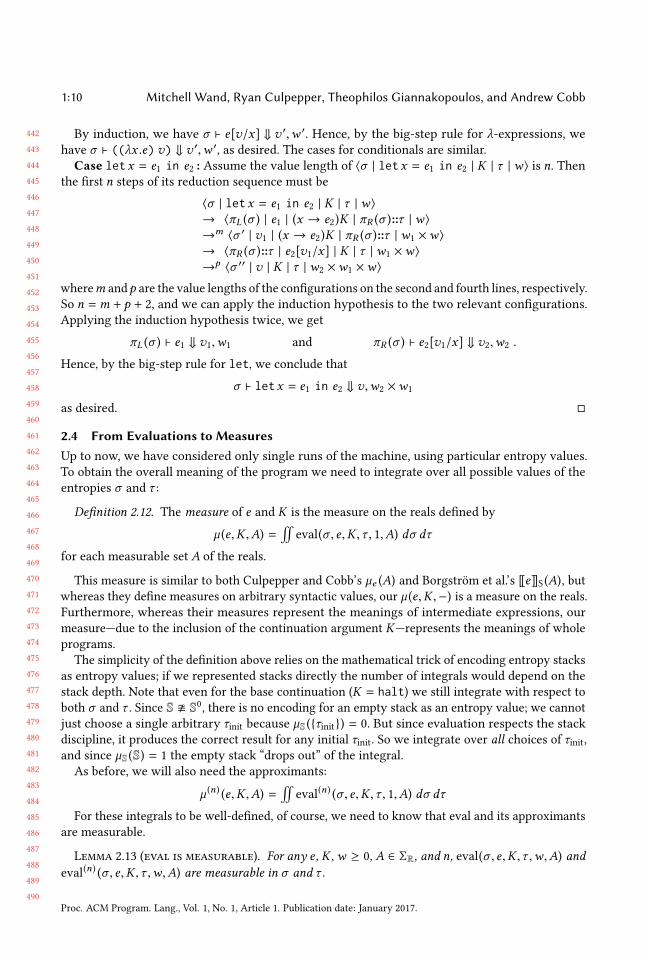
Case letx = e1 in e2 : Assume the value length of ⟨σ | letx = e1 in e2 | K | τ | w⟩ is n. Thenthe first n steps of its reduction sequence must be
⟨σ | letx = e1 in e2 | K | τ | w⟩→ ⟨πL (σ ) | e1 | (x → e2)K | πR (σ )::τ | w⟩→m ⟨σ ′ | v1 | (x → e2)K | πR (σ )::τ | w1 ×w⟩→ ⟨πR (σ )::τ | e2[v1/x] | K | τ | w1 ×w⟩→p ⟨σ ′′ | v | K | τ | w2 ×w1 ×w⟩
wherem andp are the value lengths of the configurations on the second and fourth lines, respectively.So n =m + p + 2, and we can apply the induction hypothesis to the two relevant configurations.
Applying the induction hypothesis twice, we get
πL (σ ) ⊢ e1 ⇓ v1,w1 and πR (σ ) ⊢ e2[v1/x] ⇓ v2,w2 .
Hence, by the big-step rule for let, we conclude that
σ ⊢ letx = e1 in e2 ⇓ v,w2 ×w1
as desired.
2.4 From Evaluations to MeasuresUp to now, we have considered only single runs of the machine, using particular entropy values.
To obtain the overall meaning of the program we need to integrate over all possible values of the
entropies σ and τ :
Definition 2.12. The measure of e and K is the measure on the reals defined by
µ (e,K ,A) =!
eval(σ , e,K ,τ , 1,A) dσ dτ
for each measurable set A of the reals.
This measure is similar to both Culpepper and Cobb’s µe (A) and Borgström et al.’s [[e]]S (A), butwhereas they define measures on arbitrary syntactic values, our µ (e,K ,−) is a measure on the reals.
Furthermore, whereas their measures represent the meanings of intermediate expressions, our
measure—due to the inclusion of the continuation argument K—represents the meanings of whole
programs.
The simplicity of the definition above relies on the mathematical trick of encoding entropy stacks
as entropy values; if we represented stacks directly the number of integrals would depend on the
stack depth. Note that even for the base continuation (K = halt) we still integrate with respect to
both σ and τ . Since S S0, there is no encoding for an empty stack as an entropy value; we cannot
just choose a single arbitrary τinit because µS (τinit) = 0. But since evaluation respects the stack
discipline, it produces the correct result for any initial τinit. So we integrate over all choices of τinit,and since µS (S) = 1 the empty stack “drops out” of the integral.
As before, we will also need the approximants:
µ (n) (e,K ,A) =!
eval(n) (σ , e,K ,τ , 1,A) dσ dτ
For these integrals to be well-defined, of course, we need to know that eval and its approximants
are measurable.
Lemma 2.13 (eval is measurable). For any e , K ,w ≥ 0, A ∈ ΣR, and n, eval(σ , e,K ,τ ,w,A) andeval
(n) (σ , e,K ,τ ,w,A) are measurable in σ and τ .
Proc. ACM Program. Lang., Vol. 1, No. 1, Article 1. Publication date: January 2017.
491
492
493
494
495
496
497
498
499
500
501
502
503
504
505
506
507
508
509
510
511
512
513
514
515
516
517
518
519
520
521
522
523
524
525
526
527
528
529
530
531
532
533
534
535
536
537
538
539
Contextual Equivalence for a Probabilistic Language with Continuous Random Variables andRecursion 1:11
Proof. See appendix.
The next lemma establishes some properties of µ and the approximants µ (n) . In particular, it
shows that µ is the limit of the approximants.
Lemma 2.14 (measures are monotonic). In the following, e and K range over closed expressionsand continuations, and let A range over measurable sets of reals.(1) µ (e,K ,A) ≥ 0
(2) for anym, µ (m) (e,K ,A) ≥ 0
(3) ifm ≤ n, then µ (m) (e,K ,A) ≤ µ (n) (e,K ,A) ≤ µ (e,K ,A)(4) µ (e,K ,A) = supn µ
(n) (e,K ,A)
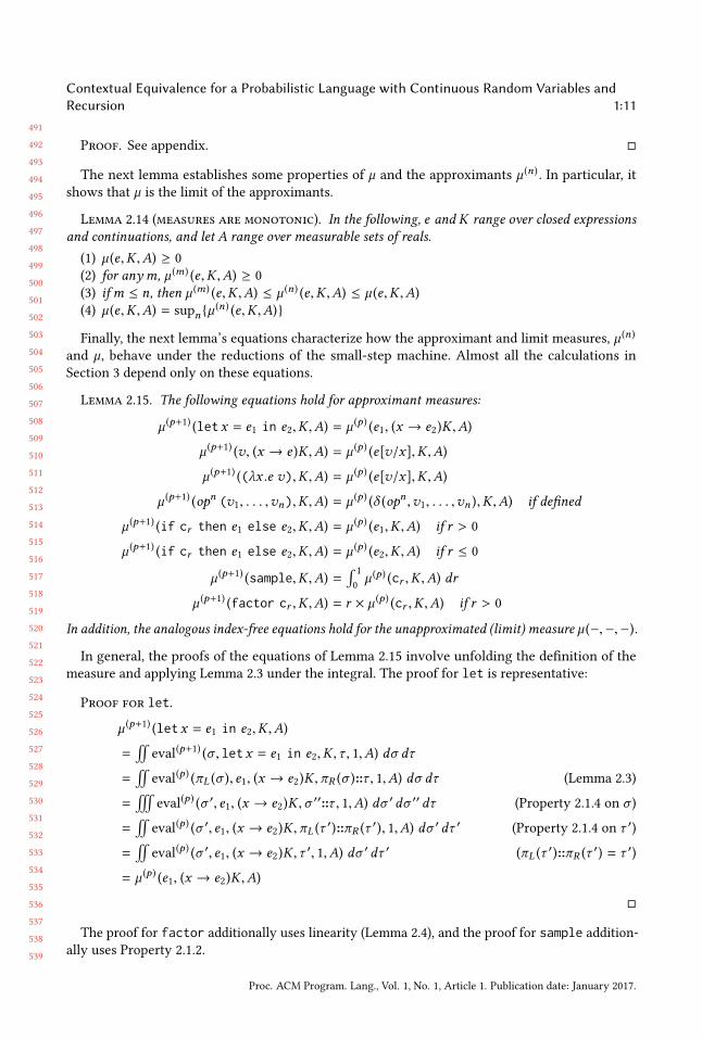
Finally, the next lemma’s equations characterize how the approximant and limit measures, µ (n)
and µ, behave under the reductions of the small-step machine. Almost all the calculations in
Section 3 depend only on these equations.
Lemma 2.15. The following equations hold for approximant measures:
µ (p+1) (letx = e1 in e2,K ,A) = µ (p ) (e1, (x → e2)K ,A)
µ (p+1) (v, (x → e )K ,A) = µ (p ) (e[v/x],K ,A)
µ (p+1) ((λx .e v),K ,A) = µ (p ) (e[v/x],K ,A)
µ (p+1) (opn (v1, . . . ,vn),K ,A) = µ (p ) (δ (opn ,v1, . . . ,vn ),K ,A) if defined
µ (p+1) (if cr then e1 else e2,K ,A) = µ (p ) (e1,K ,A) if r > 0
µ (p+1) (if cr then e1 else e2,K ,A) = µ (p ) (e2,K ,A) if r ≤ 0
µ (p+1) (sample,K ,A) =∫
1
0µ (p ) (cr ,K ,A) dr
µ (p+1) (factor cr ,K ,A) = r × µ(p ) (cr ,K ,A) if r > 0
In addition, the analogous index-free equations hold for the unapproximated (limit) measure µ (−,−,−).
In general, the proofs of the equations of Lemma 2.15 involve unfolding the definition of the
measure and applying Lemma 2.3 under the integral. The proof for let is representative:
Proof for let.
µ (p+1) (letx = e1 in e2,K ,A)
=!
eval(p+1) (σ , letx = e1 in e2,K ,τ , 1,A) dσ dτ
=!
eval(p ) (πL (σ ), e1, (x → e2)K ,πR (σ )::τ , 1,A) dσ dτ (Lemma 2.3)
=#
eval(p ) (σ ′, e1, (x → e2)K ,σ
′′::τ , 1,A) dσ ′dσ ′′dτ (Property 2.1.4 on σ )
=!
eval(p ) (σ ′, e1, (x → e2)K ,πL (τ
′)::πR (τ ′), 1,A) dσ ′dτ ′ (Property 2.1.4 on τ ′)
=!
eval(p ) (σ ′, e1, (x → e2)K ,τ
′, 1,A) dσ ′dτ ′ (πL (τ′)::πR (τ ′) = τ ′)
= µ (p ) (e1, (x → e2)K ,A)
The proof for factor additionally uses linearity (Lemma 2.4), and the proof for sample addition-
ally uses Property 2.1.2.
Proc. ACM Program. Lang., Vol. 1, No. 1, Article 1. Publication date: January 2017.
540
541
542
543
544
545
546
547
548
549
550
551
552
553
554
555
556
557
558
559
560
561
562
563
564
565
566
567
568
569
570
571
572
573
574
575
576
577
578
579
580
581
582
583
584
585
586
587
588
1:12 Mitchell Wand, Ryan Culpepper, Theophilos Giannakopoulos, and Andrew Cobb
So far, our semantics speaks directly only about the meanings of whole programs. In the following
sections, we develop a collection of relations for expressions and ultimately show that they respect
the contextual ordering relation on expression induced by the semantics of whole programs.
3 THE LOGICAL RELATIONIn this section, we will define a step-indexed logical relation on values, expressions, and continua-
tions, and we prove the Fundamental Property for our relation.
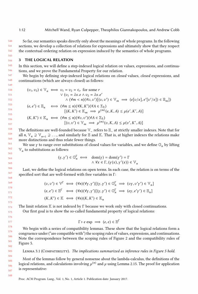
We begin by defining step-indexed logical relations on closed values, closed expressions, and
continuations (which are always closed) as follows:
(v1,v2) ∈ Vn ⇐⇒ v1 = v2 = cr for some r∨ (v1 = λx .e ∧v2 = λx .e ′
∧ (∀m < n) (∀v,v ′)[(v,v ′) ∈ Vm =⇒ (e[v/x], e ′[v ′/x]) ∈ Em])
(e, e ′) ∈ En ⇐⇒ (∀m ≤ n) (∀K ,K ′) (∀A ∈ ΣR)[(K ,K ′) ∈ Km =⇒ µ (m) (e,K ,A) ≤ µ (e ′,K ′,A)]
(K ,K ′) ∈ Kn ⇐⇒ (∀m ≤ n) (∀v,v ′) (∀A ∈ ΣR)[(v,v ′) ∈ Vm =⇒ µ (m) (v,K ,A) ≤ µ (v ′,K ′,A)]
The definitions are well-founded because V− refers to E− at strictly smaller indexes. Note that for
all n, Vn ⊇ Vn+1 ⊇ . . ., and similarly for E and K. That is, at higher indexes the relations make
more distinctions and thus relate fewer things.
We use γ to range over substitutions of closed values for variables, and we define Gn by lifting
Vn to substitutions as follows:
(γ ,γ ′) ∈ GΓn ⇐⇒ dom(γ ) = dom(γ ′) = Γ
∧ ∀x ∈ Γ, (γ (x ),γ ′(x )) ∈ Vn
Last, we define the logical relations on open terms. In each case, the relation is on terms of the
specified sort that are well-formed with free variables in Γ:
(v,v ′) ∈ VΓ ⇐⇒ (∀n) (∀γ ,γ ′)[(γ ,γ ′) ∈ GΓn =⇒ (vγ ,v ′γ ′) ∈ Vn]
(e, e ′) ∈ EΓ ⇐⇒ (∀n) (∀γ ,γ ′)[(γ ,γ ′) ∈ GΓn =⇒ (eγ , e ′γ ′) ∈ En]
(K ,K ′) ∈ K ⇐⇒ (∀n) (K ,K ′) ∈ Kn
The limit relation K is not indexed by Γ because we work only with closed continuations.
Our first goal is to show the so-called fundamental property of logical relations:
Γ ⊢ e exp =⇒ (e, e ) ∈ EΓ
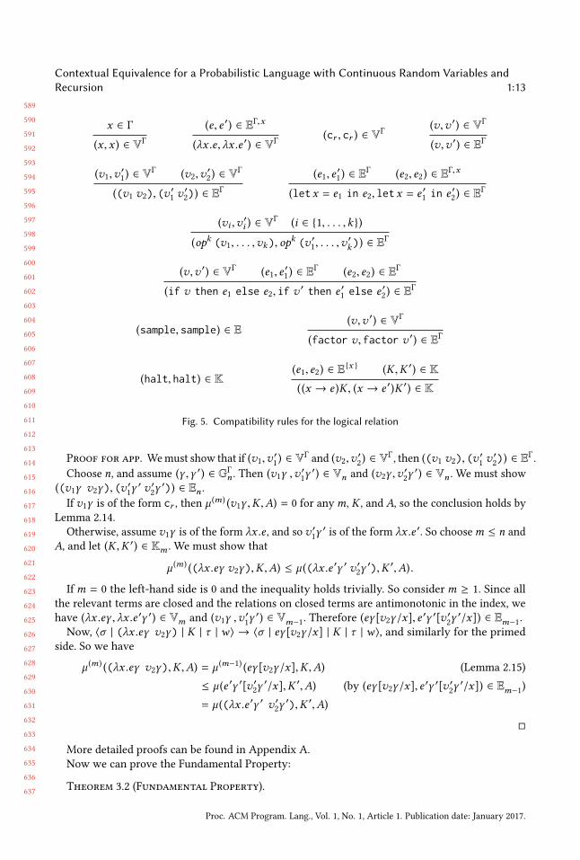
We begin with a series of compatibility lemmas. These show that the logical relations form a
congruence under (“are compatiblewith”) the scoping rules of values, expressions, and continuations.
Note the correspondence between the scoping rules of Figure 2 and the compatibility rules of
Figure 5.
Lemma 3.1 (Compatibility). The implications summarized as inference rules in Figure 5 hold.
Most of the lemmas follow by general nonsense about the lambda-calculus, the definitions of the
logical relations, and calculations involving µ (n) and µ using Lemma 2.15. The proof for application
is representative:
Proc. ACM Program. Lang., Vol. 1, No. 1, Article 1. Publication date: January 2017.
589
590
591
592
593
594
595
596
597
598
599
600
601
602
603
604
605
606
607
608
609
610
611
612
613
614
615
616
617
618
619
620
621
622
623
624
625
626
627
628
629
630
631
632
633
634
635
636
637
Contextual Equivalence for a Probabilistic Language with Continuous Random Variables andRecursion 1:13
x ∈ Γ
(x ,x ) ∈ VΓ
(e, e ′) ∈ EΓ,x
(λx .e, λx .e ′) ∈ VΓ(cr , cr ) ∈ V
Γ(v,v ′) ∈ VΓ
(v,v ′) ∈ EΓ
(v1,v′1) ∈ VΓ (v2,v
′2) ∈ VΓ
((v1 v2), (v′1v ′2)) ∈ EΓ
(e1, e′1) ∈ EΓ (e2, e2) ∈ E
Γ,x
(letx = e1 in e2, letx = e ′1in e ′
2) ∈ EΓ
(vi ,v′i ) ∈ V
Γ (i ∈ 1, . . . ,k )
(opk (v1, . . . ,vk), opk (v ′1, . . . ,v′k)) ∈ E
Γ
(v,v ′) ∈ VΓ (e1, e′1) ∈ EΓ (e2, e2) ∈ E
Γ
(if v then e1 else e2, if v ′ then e ′1else e ′
2) ∈ EΓ
(sample, sample) ∈ E(v,v ′) ∈ VΓ
(factor v, factor v ′) ∈ EΓ
(halt, halt) ∈ K(e1, e2) ∈ E
x (K ,K ′) ∈ K
((x → e )K , (x → e ′)K ′) ∈ K
Fig. 5. Compatibility rules for the logical relation
Proof for app. Wemust show that if (v1,v′1) ∈ VΓ
and (v2,v′2) ∈ VΓ
, then ((v1 v2), (v′1v ′2)) ∈ EΓ .
Choose n, and assume (γ ,γ ′) ∈ GΓn . Then (v1γ ,v
′1γ ′) ∈ Vn and (v2γ ,v
′2γ ′) ∈ Vn . We must show
((v1γ v2γ), (v′1γ ′ v ′
2γ ′)) ∈ En .
If v1γ is of the form cr , then µ (m) (v1γ ,K ,A) = 0 for anym, K , and A, so the conclusion holds by
Lemma 2.14.
Otherwise, assume v1γ is of the form λx .e , and so v ′1γ ′ is of the form λx .e ′. So choosem ≤ n and
A, and let (K ,K ′) ∈ Km . We must show that
µ (m) ((λx .eγ v2γ),K ,A) ≤ µ ((λx .e ′γ ′ v ′2γ ′),K ′,A).
Ifm = 0 the left-hand side is 0 and the inequality holds trivially. So considerm ≥ 1. Since all
the relevant terms are closed and the relations on closed terms are antimonotonic in the index, we
have (λx .eγ , λx .e ′γ ′) ∈ Vm and (v1γ ,v′1γ ′) ∈ Vm−1. Therefore (eγ [v2γ/x], e
′γ ′[v ′2γ ′/x]) ∈ Em−1.
Now, ⟨σ | (λx .eγ v2γ) | K | τ | w⟩ → ⟨σ | eγ [v2γ/x] | K | τ | w⟩, and similarly for the primed
side. So we have
µ (m) ((λx .eγ v2γ),K ,A) = µ (m−1) (eγ [v2γ/x],K ,A) (Lemma 2.15)
≤ µ (e ′γ ′[v ′2γ ′/x],K ′,A) (by (eγ [v2γ/x], e
′γ ′[v ′2γ ′/x]) ∈ Em−1)
= µ ((λx .e ′γ ′ v ′2γ ′),K ′,A)
More detailed proofs can be found in Appendix A.
Now we can prove the Fundamental Property:
Theorem 3.2 (Fundamental Property).
Proc. ACM Program. Lang., Vol. 1, No. 1, Article 1. Publication date: January 2017.
638
639
640
641
642
643
644
645
646
647
648
649
650
651
652
653
654
655
656
657
658
659
660
661
662
663
664
665
666
667
668
669
670
671
672
673
674
675
676
677
678
679
680
681
682
683
684
685
686
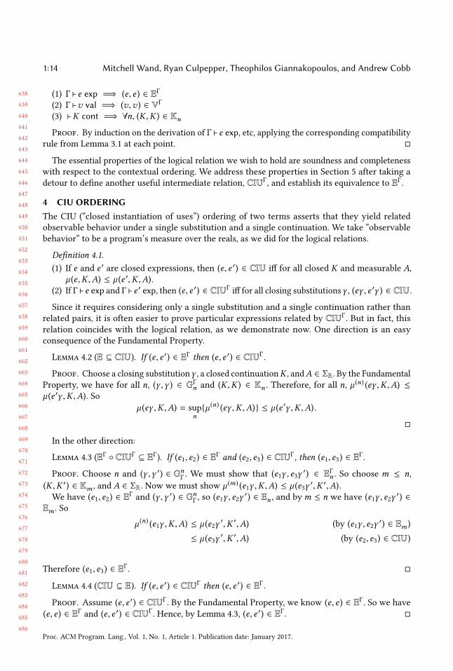
1:14 Mitchell Wand, Ryan Culpepper, Theophilos Giannakopoulos, and Andrew Cobb
(1) Γ ⊢ e exp =⇒ (e, e ) ∈ EΓ
(2) Γ ⊢v val =⇒ (v,v ) ∈ VΓ
(3) ⊢K cont =⇒ ∀n, (K ,K ) ∈ Kn
Proof. By induction on the derivation of Γ ⊢ e exp, etc, applying the corresponding compatibility
rule from Lemma 3.1 at each point.
The essential properties of the logical relation we wish to hold are soundness and completeness
with respect to the contextual ordering. We address these properties in Section 5 after taking a
detour to define another useful intermediate relation, CIUΓ, and establish its equivalence to EΓ .
4 CIU ORDERINGThe CIU (“closed instantiation of uses”) ordering of two terms asserts that they yield related
observable behavior under a single substitution and a single continuation. We take “observable
behavior” to be a program’s measure over the reals, as we did for the logical relations.
Definition 4.1.(1) If e and e ′ are closed expressions, then (e, e ′) ∈ CIU iff for all closed K and measurable A,
µ (e,K ,A) ≤ µ (e ′,K ,A).(2) If Γ ⊢ e exp and Γ ⊢ e ′ exp, then (e, e ′) ∈ CIUΓ
iff for all closing substitutionsγ , (eγ , e ′γ ) ∈ CIU.
Since it requires considering only a single substitution and a single continuation rather than
related pairs, it is often easier to prove particular expressions related by CIUΓ. But in fact, this
relation coincides with the logical relation, as we demonstrate now. One direction is an easy
consequence of the Fundamental Property.
Lemma 4.2 (E ⊆ CIU). If (e, e ′) ∈ EΓ then (e, e ′) ∈ CIUΓ .
Proof. Choose a closing substitutionγ , a closed continuationK , andA ∈ ΣR. By the Fundamental
Property, we have for all n, (γ ,γ ) ∈ GΓn and (K ,K ) ∈ Kn . Therefore, for all n, µ
(n) (eγ ,K ,A) ≤µ (e ′γ ,K ,A). So
µ (eγ ,K ,A) = sup
nµ (n) (eγ ,K ,A) ≤ µ (e ′γ ,K ,A).
In the other direction:
Lemma 4.3 (EΓ CIUΓ ⊆ EΓ). If (e1, e2) ∈ EΓ and (e2, e3) ∈ CIUΓ , then (e1, e3) ∈ E
Γ .
Proof. Choose n and (γ ,γ ′) ∈ GnΓ . We must show that (e1γ , e3γ′) ∈ EΓn . So choose m ≤ n,
(K ,K ′) ∈ Km , and A ∈ ΣR. Now we must show µ (m) (e1γ ,K ,A) ≤ µ (e3γ′,K ′,A).
We have (e1, e2) ∈ EΓand (γ ,γ ′) ∈ GnΓ , so (e1γ , e2γ
′) ∈ En , and bym ≤ n we have (e1γ , e2γ′) ∈
Em . So
µ (n) (e1γ ,K ,A) ≤ µ (e2γ′,K ′,A) (by (e1γ , e2γ
′) ∈ Em )
≤ µ (e3γ′,K ′,A) (by (e2, e3) ∈ CIU)
Therefore (e1, e3) ∈ EΓ.
Lemma 4.4 (CIU ⊆ E). If (e, e ′) ∈ CIUΓ then (e, e ′) ∈ EΓ .
Proof. Assume (e, e ′) ∈ CIUΓ. By the Fundamental Property, we know (e, e ) ∈ EΓ . So we have
(e, e ) ∈ EΓ and (e, e ′) ∈ CIUΓ. Hence, by Lemma 4.3, (e, e ′) ∈ EΓ .
Proc. ACM Program. Lang., Vol. 1, No. 1, Article 1. Publication date: January 2017.
687
688
689
690
691
692
693
694
695
696
697
698
699
700
701
702
703
704
705
706
707
708
709
710
711
712
713
714
715
716
717
718
719
720
721
722
723
724
725
726
727
728
729
730
731
732
733
734
735
Contextual Equivalence for a Probabilistic Language with Continuous Random Variables andRecursion 1:15
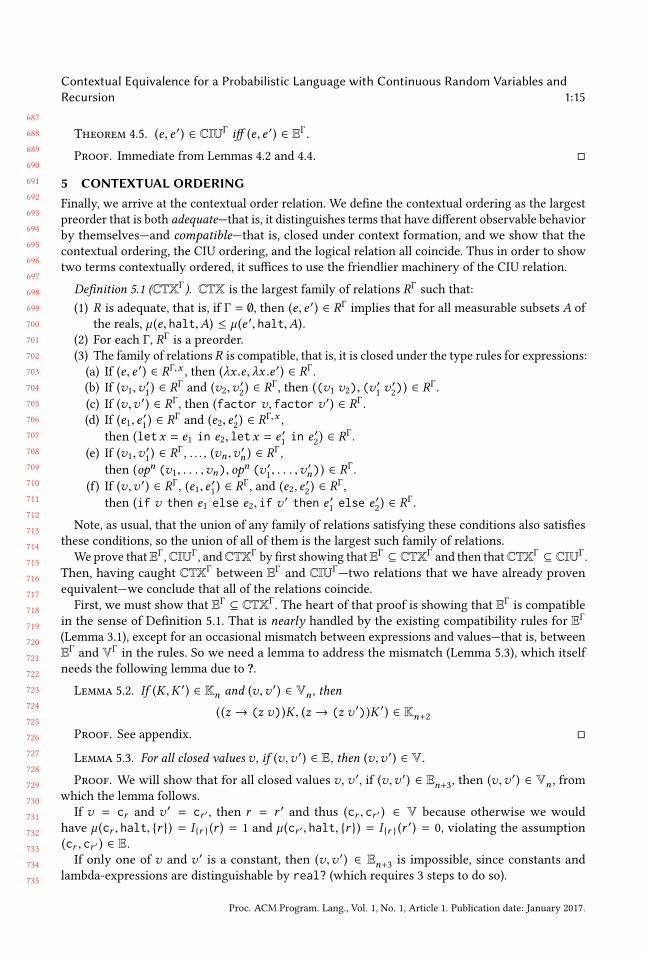
Theorem 4.5. (e, e ′) ∈ CIUΓ iff (e, e ′) ∈ EΓ .
Proof. Immediate from Lemmas 4.2 and 4.4.
5 CONTEXTUAL ORDERINGFinally, we arrive at the contextual order relation. We define the contextual ordering as the largest
preorder that is both adequate—that is, it distinguishes terms that have different observable behavior
by themselves—and compatible—that is, closed under context formation, and we show that the
contextual ordering, the CIU ordering, and the logical relation all coincide. Thus in order to show
two terms contextually ordered, it suffices to use the friendlier machinery of the CIU relation.
Definition 5.1 (CTXΓ). CTX is the largest family of relations RΓsuch that:
(1) R is adequate, that is, if Γ = ∅, then (e, e ′) ∈ RΓimplies that for all measurable subsets A of
the reals, µ (e, halt,A) ≤ µ (e ′, halt,A).(2) For each Γ, RΓ
is a preorder.
(3) The family of relations R is compatible, that is, it is closed under the type rules for expressions:
(a) If (e, e ′) ∈ RΓ,x, then (λx .e, λx .e ′) ∈ RΓ
.
(b) If (v1,v′1) ∈ RΓ
and (v2,v′2) ∈ RΓ
, then ((v1 v2), (v′1v ′2)) ∈ RΓ
.
(c) If (v,v ′) ∈ RΓ, then (factor v, factor v ′) ∈ RΓ
.
(d) If (e1, e′1) ∈ RΓ
and (e2, e′2) ∈ RΓ,x
,
then (letx = e1 in e2, letx = e ′1in e ′
2) ∈ RΓ
.
(e) If (v1,v′1) ∈ RΓ
, . . . , (vn ,v′n ) ∈ R
Γ,
then (opn (v1, . . . ,vn), opn (v ′1, . . . ,v′n)) ∈ R
Γ.
(f) If (v,v ′) ∈ RΓ, (e1, e
′1) ∈ RΓ
, and (e2, e′2) ∈ RΓ
,
then (if v then e1 else e2, if v ′ then e ′1else e ′
2) ∈ RΓ
.
Note, as usual, that the union of any family of relations satisfying these conditions also satisfies
these conditions, so the union of all of them is the largest such family of relations.
We prove thatEΓ ,CIUΓ, andCTXΓ
by first showing thatEΓ ⊆ CTXΓand then thatCTXΓ ⊆ CIUΓ
.
Then, having caught CTXΓbetween EΓ and CIUΓ
—two relations that we have already proven
equivalent—we conclude that all of the relations coincide.
First, we must show that EΓ ⊆ CTXΓ. The heart of that proof is showing that EΓ is compatible
in the sense of Definition 5.1. That is nearly handled by the existing compatibility rules for EΓ
(Lemma 3.1), except for an occasional mismatch between expressions and values—that is, between
EΓ and VΓin the rules. So we need a lemma to address the mismatch (Lemma 5.3), which itself
needs the following lemma due to ?.
Lemma 5.2. If (K ,K ′) ∈ Kn and (v,v ′) ∈ Vn , then
((z → (z v))K , (z → (z v ′))K ′) ∈ Kn+2
Proof. See appendix.
Lemma 5.3. For all closed values v , if (v,v ′) ∈ E, then (v,v ′) ∈ V.
Proof. We will show that for all closed values v , v ′, if (v,v ′) ∈ En+3, then (v,v ′) ∈ Vn , fromwhich the lemma follows.
If v = cr and v ′ = cr ′ , then r = r ′ and thus (cr , cr ′ ) ∈ V because otherwise we would
have µ (cr , halt, r ) = I r (r ) = 1 and µ (cr ′, halt, r ) = I r (r′) = 0, violating the assumption
(cr , cr ′ ) ∈ E.If only one of v and v ′ is a constant, then (v,v ′) ∈ En+3 is impossible, since constants and
lambda-expressions are distinguishable by real? (which requires 3 steps to do so).
Proc. ACM Program. Lang., Vol. 1, No. 1, Article 1. Publication date: January 2017.
736
737
738
739
740
741
742
743
744
745
746
747
748
749
750
751
752
753
754
755
756
757
758
759
760
761
762
763
764
765
766
767
768
769
770
771
772
773
774
775
776
777
778
779
780
781
782
783
784
1:16 Mitchell Wand, Ryan Culpepper, Theophilos Giannakopoulos, and Andrew Cobb
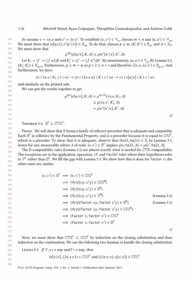
So assume v = λx .e and v ′ = λx .e ′. To establish (v,v ′) ∈ Vn , choosem < n and (u,u ′) ∈ Vm .We must show that (e[u/x], e ′[u ′/x]) ∈ Em . To do that, choose p ≤ m, (K ,K ′) ∈ Kp , and A ∈ ΣR.We must show that
µ (p ) (e[u/x],K ,A) ≤ µ (e ′[u ′/x],K ′,A)
LetK1 = ( f → (f u))K andK ′1= ( f → (f u ′))K ′. Bymonotonicity, (u,u ′) ∈ Vp . By Lemma 5.2,
(K ′1,K ′
1) ∈ Kp+2. Furthermore, p ≤ m < n, so p + 2 ≤ n + 1 and therefore (λx .e, λx .e ′) ∈ Ep+2. And
furthermore, we have
⟨σ | λx .e | K1 | τ | w⟩ → ⟨σ | (λx .e u) | K | τ | w⟩ → ⟨σ | e[u/x] | K | τ | w⟩
and similarly on the primed side.
We can put the results together to get
µ (p ) (e[u/x],K ,A) = µ (p+2) (λx .e,K1,A)
≤ µ (λx .e ′,K ′1,A)
= µ (e ′[u ′/x],K ′,A)
Theorem 5.4. EΓ ⊆ CTXΓ .
Proof. Wewill show that E forms a family of reflexive preorders that is adequate and compatible.
Each EΓ is reflexive by the Fundamental Property, and is a preorder because it is equal to CIUΓ,
which is a preorder. To show that it is adequate, observe that (halt, halt) ∈ K by Lemma 3.1,
hence for any measurable subset A of reals, (e, e ′) ∈ EΓ implies µ (e, halt,A) = µ (e ′, halt,A).The E-compatibility rules (Lemma 3.1) are almost exactly what is needed for CTX-compatibility.
The exceptions are in the application, operation, if, and factor rules where their hypotheses referto VΓ
rather than EΓ . We fill the gap with Lemma 5.3. We show how this is done for factor v ; theother cases are similar.
(v,v ′) ∈ EΓ =⇒ (v,v ′) ∈ CIUΓ
=⇒ (∀γ ) ((vγ ,v ′γ ) ∈ CIU∅)
=⇒ (∀γ ) ((vγ ,v ′γ ) ∈ E∅)
=⇒ (∀γ ) ((vγ ,v ′γ ) ∈ V∅) (Lemma 5.3)
=⇒ (∀γ ) ((factor vγ , factor v ′γ ) ∈ E∅) (Lemma 3.1)
=⇒ (∀γ ) ((factor vγ , factor v ′γ ) ∈ CIU∅)
=⇒ (factor v, factor v ′) ∈ CIUΓ
=⇒ (factor v, factor v ′) ∈ EΓ
Next, we must show that CTXΓ ⊆ CIUΓby induction on the closing substitution and then
induction on the continuation. We use the following two lemmas to handle the closing substitution.
Lemma 5.5. If Γ,x ⊢ e exp and Γ ⊢v exp, then
(e[v/x], (λx .e v)) ∈ CIUΓ and ((λx .e v), e[v/x]) ∈ CIUΓ .
Proc. ACM Program. Lang., Vol. 1, No. 1, Article 1. Publication date: January 2017.
785
786
787
788
789
790
791
792
793
794
795
796
797
798
799
800
801
802
803
804
805
806
807
808
809
810
811
812
813
814
815
816
817
818
819
820
821
822
823
824
825
826
827
828
829
830
831
832
833
Contextual Equivalence for a Probabilistic Language with Continuous Random Variables andRecursion 1:17
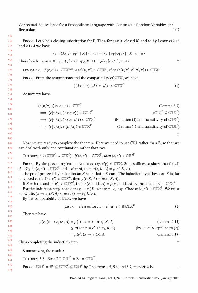
Proof. Let γ be a closing substitution for Γ. Then for any σ , closed K , andw , by Lemmas 2.15
and 2.14.4 we have
⟨σ | (λx .eγ vγ) | K | τ | w⟩ → ⟨σ | eγ [vγ/x] | K | τ | w⟩
Therefore for any A ∈ ΣR, µ ((λx .eγ vγ),K ,A) = µ (eγ [vγ/x],K ,A).
Lemma 5.6. If (e, e ′) ∈ CTXΓ,x , and (v,v ′) ∈ CTXΓ , then (e[v/x], e ′[v ′/x]) ∈ CTXΓ .
Proof. From the assumptions and the compatibility of CTX, we have
((λx .e v), (λx .e ′ v ′)) ∈ CTXΓ(1)
So now we have:
(e[v/x], (λx .e v)) ∈ CIUΓ(Lemma 5.5)
=⇒ (e[v/x], (λx .e v)) ∈ CTXΓ(CIUΓ ⊆ CTXΓ
)
=⇒ (e[v/x], (λx .e ′ v ′)) ∈ CTXΓ(Equation (1) and transitivity of CTXΓ
)
=⇒ (e[v/x], e ′[v ′/x]) ∈ CTXΓ(Lemma 5.5 and transitivity of CTXΓ
)
Now we are ready to complete the theorem. Here we need to use CIU rather than E, so that we
can deal with only one continuation rather than two.
Theorem 5.7 (CTXΓ ⊆ CIUΓ). If (e, e ′) ∈ CTXΓ , then (e, e ′) ∈ CIUΓ
Proof. By the preceding lemma, we have (eγ , e ′γ ) ∈ CTX. So it suffices to show that for all
A ∈ ΣR, if (e, e′) ∈ CTX∅ and ⊢K cont, then µ (e,K ,A) = µ (e ′,K ,A).
The proof proceeds by induction on K such that ⊢K cont. The induction hypothesis on K is: for
all closed e , e ′, if (e, e ′) ∈ CTX∅, then µ (e,K ,A) = µ (e ′,K ,A).If K = halt and (e, e ′) ∈ CTX∅, then µ (e, halt,A) = µ (e ′, halt,A) by the adequacy of CTX∅.
For the induction step, consider (x → e1)K , where x ⊢ e1 exp. Choose (e, e ′) ∈ CTX∅. We must
show µ (e, (x → e1)K ,A) ≤ µ (e ′, (x → e1)K ,A).By the compatibility of CTX, we have
(letx = e in e1, letx = e ′ in e1) ∈ CTX∅
(2)
Then we have
µ (e, (x → e1)K ,A) = µ (letx = e in e1,K ,A) (Lemma 2.15)
≤ µ (letx = e ′ in e1,K ,A) (by IH at K , applied to (2))
= µ (e ′, (x → e1)K ,A) (Lemma 2.15)
Thus completing the induction step.
Summarizing the results:
Theorem 5.8. For all Γ, CIUΓ = EΓ = CTXΓ .
Proof. CIUΓ = EΓ ⊆ CTXΓ ⊆ CIUΓby Theorems 4.5, 5.4, and 5.7, respectively.
Proc. ACM Program. Lang., Vol. 1, No. 1, Article 1. Publication date: January 2017.
834
835
836
837
838
839
840
841
842
843
844
845
846
847
848
849
850
851
852
853
854
855
856
857
858
859
860
861
862
863
864
865
866
867
868
869
870
871
872
873
874
875
876
877
878
879
880
881
882
1:18 Mitchell Wand, Ryan Culpepper, Theophilos Giannakopoulos, and Andrew Cobb
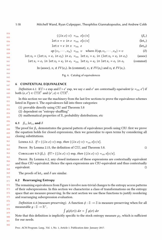
((λx .e) v) =ctx e[v/x] (βv )
letx = v in e =ctx e[v/x] (letv )
letx = e in x =ctx e (letid )
op (v1, · · · ,vn) =ctx v where δ (op,v1, · · · ,vn ) = v (δ )
letx2 = (letx1 = e1 in e2) in e3 =ctx letx1 = e1 in (letx2 = e2 in e3) (assoc)
letx1 = e1 in letx2 = e2 in e3 =ctx letx2 = e2 in letx1 = e1 in e3 (commut)
In (assoc), x1 < FV (e3). In (commut), x1 < FV (e2) and x2 < FV (e1).
Fig. 6. Catalog of equivalences
6 CONTEXTUAL EQUIVALENCEDefinition 6.1. If Γ ⊢ e exp and Γ ⊢ e ′ exp, we say e and e ′ are contextually equivalent (e =ctx e ′) if
both (e, e ′) ∈ CTXΓand (e ′, e ) ∈ CTXΓ
.
In this section we use the machinery from the last few sections to prove the equivalence schemes
listed in Figure 6. The equivalences fall into three categories:
(1) provable directly using CIU and Theorem 5.8
(2) dependent on “entropy-shuffling”
(3) mathematical properties of R, probability distributions, etc
6.1 βv , letv , and δ
The proof for βv demonstrates the general pattern of equivalence proofs using CIU: first we prove
the equation holds for closed expressions, then we generalize to open terms by considering all
closing substitutions.
Lemma 6.2. If ⊢ ((λx .e) v) exp, then ((λx .e) v) =ctx e[v/x].
Proof. By Lemma 2.15, the definition of CIU, and Theorem 5.8.
Corollary 6.3 (βv ). If Γ ⊢ ((λx .e) v) exp, then ((λx .e) v) =ctx e[v/x].
Proof. By Lemma 6.2, any closed instances of these expressions are contextually equivalent
and thus CIU-equivalent. Hence the open expressions are CIU-equivalent and thus contextually
equivalent.
The proofs of letv and δ are similar.
6.2 Rearranging EntropyThe remaining equivalences from Figure 6 involve non-trivial changes to the entropy access patterns
of their subexpressions. In this section we characterize a class of transformations on the entropy
space that are measure-preserving. In the next section we use these functions to justify reordering
and rearranging subexpression evaluation.
Definition 6.4 (measure-preserving). A function ϕ : S → S is measure-preserving when for all
measurable д : S→ R+, ∫д(ϕ (σ )) dσ =
∫д(σ ) dσ
Note that this definition is implicitly specific to the stock entropy measure µS, which is sufficient
for our needs.
Proc. ACM Program. Lang., Vol. 1, No. 1, Article 1. Publication date: January 2017.
883
884
885
886
887
888
889
890
891
892
893
894
895
896
897
898
899
900
901
902
903
904
905
906
907
908
909
910
911
912
913
914
915
916
917
918
919
920
921
922
923
924
925
926
927
928
929
930
931
Contextual Equivalence for a Probabilistic Language with Continuous Random Variables andRecursion 1:19
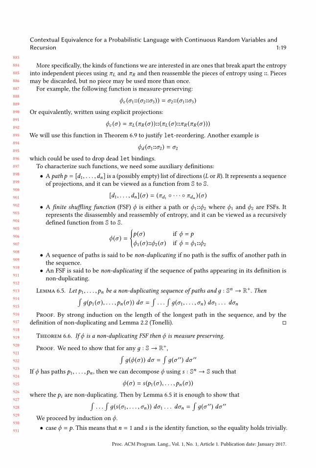
More specifically, the kinds of functions we are interested in are ones that break apart the entropy
into independent pieces using πL and πR and then reassemble the pieces of entropy using ::. Piecesmay be discarded, but no piece may be used more than once.
For example, the following function is measure-preserving:
ϕc (σ1::(σ2::σ3)) = σ2::(σ1::σ3)
Or equivalently, written using explicit projections:
ϕc (σ ) = πL (πR (σ ))::(πL (σ )::πR (πR (σ )))
We will use this function in Theorem 6.9 to justify let-reordering. Another example is
ϕd (σ1::σ2) = σ2
which could be used to drop dead let bindings.To characterize such functions, we need some auxiliary definitions:
• A path p = [d1, . . . ,dn] is a (possibly empty) list of directions (L or R). It represents a sequenceof projections, and it can be viewed as a function from S to S.
[d1, . . . ,dn](σ ) = (πd1 · · · πdn ) (σ )
• A finite shuffling function (FSF) ϕ is either a path or ϕ1::ϕ2 where ϕ1 and ϕ2 are FSFs. It
represents the disassembly and reassembly of entropy, and it can be viewed as a recursively
defined function from S to S.
ϕ (σ ) =
p (σ ) if ϕ = p
ϕ1 (σ )::ϕ2 (σ ) if ϕ = ϕ1::ϕ2
• A sequence of paths is said to be non-duplicating if no path is the suffix of another path in
the sequence.
• An FSF is said to be non-duplicating if the sequence of paths appearing in its definition is
non-duplicating.
Lemma 6.5. Let p1, . . . ,pn be a non-duplicating sequence of paths and д : Sn → R+. Then∫д(p1 (σ ), . . . ,pn (σ )) dσ =
∫. . .∫д(σ1, . . . ,σn ) dσ1 . . . dσn
Proof. By strong induction on the length of the longest path in the sequence, and by the
definition of non-duplicating and Lemma 2.2 (Tonelli).
Theorem 6.6. If ϕ is a non-duplicating FSF then ϕ is measure preserving.
Proof. We need to show that for any д : S→ R+,∫д(ϕ (σ )) dσ =
∫д(σ ′′) dσ ′′
If ϕ has paths p1, . . . ,pn , then we can decompose ϕ using s : Sn → S such that
ϕ (σ ) = s (p1 (σ ), . . . ,pn (σ ))
where the pi are non-duplicating. Then by Lemma 6.5 it is enough to show that∫. . .∫д(s (σ1, . . . ,σn )) dσ1 . . . dσn =
∫д(σ ′′) dσ ′′
We proceed by induction on ϕ.
• case ϕ = p. This means that n = 1 and s is the identity function, so the equality holds trivially.
Proc. ACM Program. Lang., Vol. 1, No. 1, Article 1. Publication date: January 2017.

932
933
934
935
936
937
938
939
940
941
942
943
944
945
946
947
948
949
950
951
952
953
954
955
956
957
958
959
960
961
962
963
964
965
966
967
968
969
970
971
972
973
974
975
976
977
978
979
980
1:20 Mitchell Wand, Ryan Culpepper, Theophilos Giannakopoulos, and Andrew Cobb
• case ϕ = ϕ1::ϕ2. If m is the number of paths in ϕ1, then there must be s1 : Sm → S ands2 : S
n−m → S such that
s (σ1, . . . ,σm ,σm+1, . . . ,σn ) = s1 (σ1, . . . ,σm )::s2 (σm+1, . . . ,σn )
We can conclude that∫. . .∫д(s (σ1, . . . ,σn )) dσ1 . . . dσn
=∫. . .∫д(s1 (σ1, . . . ,σm )::s2 (σm+1, . . . ,σn )) dσ1 . . . dσn
=!
д(σ ::σ ′) dσ dσ ′ (IH twice)
=∫д(σ ′′) dσ ′′ (Property 2.1(4))
6.3 Equivalences that depend on rearranging entropyWe first prove a general theorem relating value-preserving transformations on the entropy space:
Theorem 6.7. Let e and e ′ be closed expressions, and let ϕ : S → S be a measure-preservingtransformation such that for all σ , K , τ , and A
eval(σ , e,K ,τ , 1,A) ≤ eval(ϕ (σ ), e ′,K ,τ , 1,A)
Then (e, e ′) ∈ CTX.
Proof. Without loss of generality, assume e and e ′ are closed (otherwise apply a closing substi-
tution). By Theorem 5.8, it is sufficient to show that for any K and A, µ (e,K ,A) ≤ µ (e ′,K ,A). We
calculate:
µ (e,K ,A) =!
eval(σ , e,K ,τ , 1,A) dσ dτ
≤!
eval(ϕ (σ ), e ′,K ,τ , 1,A) dσ dτ
=!
eval(σ , e ′,K ,τ , 1,A) dσ dτ (ϕ is measure-preserving)
= µ (e ′,K ,A)
Theorem 6.8. Let e and e ′ be closed expressions, and let ϕ : S → S be a measure-preservingtransformation such that for all v andw ,
σ ⊢ e ⇓ v,w =⇒ ϕ (σ ) ⊢ e ′ ⇓ v,w .
Then (e, e ′) ∈ CTX.
Proof. We will use Theorem 6.7. Assume eval(σ , e,K ,τ , 1,A) = r > 0. Hence by Theorem 2.11,
there exist quantities v ′,w ′, σ ′, and τ ′ such that
⟨σ | e | K | τ | 1⟩ →∗ ⟨σ ′ | v ′ | halt | τ ′ | r ⟩
with v ′ ∈ A. By Theorem 2.11 there exist v ′′, σ ′′, andw ′′ such that
σ ⊢ e ⇓ v ′′,w ′′ and ⟨σ ′′ | v ′′ | K | τ | w ′′⟩ →∗ ⟨σ ′ | v ′ | halt | τ ′ | r ⟩
By the assumption of the theorem, we have ϕ (σ ) ⊢ e ′ ⇓ v ′′,w ′′.Therefore, by Theorem 2.5, there is a σ ′′′ such that
⟨σ ′ | e | K | t | 1⟩ →∗ ⟨σ ′′′ | v ′′ | K | τ | w ′′⟩
Proc. ACM Program. Lang., Vol. 1, No. 1, Article 1. Publication date: January 2017.
981
982
983
984
985
986
987
988
989
990
991
992
993
994
995
996
997
998
999
1000
1001
1002
1003
1004
1005
1006
1007
1008
1009
1010
1011
1012
1013
1014
1015
1016
1017
1018
1019
1020
1021
1022
1023
1024
1025
1026
1027
1028
1029
Contextual Equivalence for a Probabilistic Language with Continuous Random Variables andRecursion 1:21
We claim that eval(ϕ (s ), e ′,K ,τ , 1,A) = r .We proceed by cases onK .We have ⟨σ ′′ | v ′′ | K | τ | w ′′⟩ →∗
⟨ϕ (s ) | v ′ | halt | τ ′′ | r ⟩. If K = halt, this reduction must have length 0. Therefore v ′′ = v ′ ∈ Aandw ′′ = r , so eval(ϕ (s ), e ′,K ,τ , 1,A) = r .Otherwise assume K = (x → e3)K
′. Then both ⟨σ ′′ | v” | K | t | w ′′⟩ and ⟨σ ′′′ | v” | K | t | w ′′⟩
take a step to ⟨πL (τ ) | e3[v′′/x] | K ′ | πR (τ ) | w
′′⟩, whence eval(ϕ (s ), e ′,K ,τ , 1,A) = eval(σ , e,K ,τ , 1,A) =r , as desired, thus establishing the requirement of Theorem 6.7.
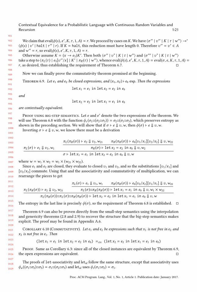
Now we can finally prove the commutativity theorem promised at the beginning.
Theorem 6.9. Let e1 and e2 be closed expressions, and x1,x2 ⊢ e0 exp. Then the expressions
letx1 = e1 in letx2 = e2 in e0
andletx2 = e2 in letx1 = e1 in e0
are contextually equivalent.
Proof using big-step semantics. Let e and e ′ denote the two expressions of the theorem. We
will use Theorem 6.8 with the function ϕc (σ1::(σ2::σ3)) = σ2::(σ1::σ3), which preserves entropy as
shown in the preceding section. We will show that if σ ⊢ e ⇓ v,w , then ϕ (σ ) ⊢ e ⇓ v,w .
Inverting σ ⊢ e ⇓ v,w , we know there must be a derivation
πL (σ ) ⊢ e1 ⇓ v1,w1
πL (πR (σ )) ⊢ e2 ⇓ v2,w21 πR (πR (σ )) ⊢ e0[v1/x1][v2/x2] ⇓ v,w22
πR (σ ) ⊢ letx2 = e2 in e0 ⇓ v,w2
σ ⊢ letx1 = e1 in letx2 = e2 in e0 ⇓ v,w
wherew = w1 ×w2 = w1 × (w21 ×w22).Since e1 and e2 are closed, they evaluate to closed v1 and v2, and so the substitutions [v1/x1] and
[v2/x2] commute. Using that and the associativity and commutativity of multiplication, we can
rearrange the pieces to get
πL (πR (σ )) ⊢ e2 ⇓ v2,w21
πL (σ ) ⊢ e1 ⇓ v1,w1 πR (πR (σ )) ⊢ e0[v2/x2][v1/x1] ⇓ v,w22
πL (σ )::πR (πR (σ )) ⊢ letx1 = e1 in e0 ⇓ v,w1 ×w22
πL (πR (σ ))::πL (σ )::πR (πR (σ )) ⊢ letx2 = e2 in letx1 = e1 in e0 ⇓ v,w
The entropy in the last line is precisely ϕ (σ ), so the requirement of Theorem 6.8 is established.
Theorem 6.9 can also be proven directly from the small-step semantics using the interpolation
and genericity theorems (2.8 and 2.9) to recover the structure that the big-step semantics makes
explicit. The proof may be found in Appendix A.6.
Corollary 6.10 (Commutativity). Let e1 and e2 be expressions such that x1 is not free in e2 andx2 is not free in e1. Then
(letx1 = e1 in letx2 = e2 in e0) =ctx (letx2 = e2 in letx1 = e1 in e0)
Proof. Same as Corollary 6.3: since all of the closed instances are equivalent by Theorem 6.9,
the open expressions are equivalent.
The proofs of let-associativity and letid follow the same structure, except that associativity uses
ϕa ((σ1::σ2)::σ3) = σ1::(σ2::σ3) and letid uses ϕi (σ1::σ2) = σ1.
Proc. ACM Program. Lang., Vol. 1, No. 1, Article 1. Publication date: January 2017.

1030
1031
1032
1033
1034
1035
1036
1037
1038
1039
1040
1041
1042
1043
1044
1045
1046
1047
1048
1049
1050
1051
1052
1053
1054
1055
1056
1057
1058
1059
1060
1061
1062
1063
1064
1065
1066
1067
1068
1069
1070
1071
1072
1073
1074
1075
1076
1077
1078
1:22 Mitchell Wand, Ryan Culpepper, Theophilos Giannakopoulos, and Andrew Cobb
6.4 Quasi-denotational ReasoningIn this section we give a powerful “quasi-denotational” reasoning tool that shows that if two
expressions are denote the same measure, they are contextually equivalent. This allows us to import
mathematical facts about real arithmetic and probability distributions.
To support this kind of reasoning, we need a notion of measure for a (closed) expression indepen-
dent of a program continuation. We define µ (e,−) as a measure over arbitrary syntactic values—notjust real numbers as with µ (e,K ,−). This measure corresponds directly to the µe of ? and [[e]]S of ?.The definition of µ uses a generalization of eval from measurable sets of reals (A) to measurable
sets of syntactic values (V ). This requires a measurable space for syntactic values; we take the
construction of ?, Figure 5 mutatis mutandis.
Definition 6.11.
µ (e,V ) =!
eval(σ , e, halt,τ , 1,V ) dσ dτ
eval(σ , e,K ,τ ,w,V ) =
w ′ if ⟨σ | e | K | τ | w⟩ →∗ ⟨σ ′ | v | halt | τ ′ | w ′⟩,
where v ∈ V
0 otherwise
Our goal is to relate an expression’s measure µ (e,−) with the measure of that expression with a
program continuation (µ (e,K ,−)). Then if two expressions have the same measures, we can use
CIU to show them contextually equivalent.
First we need a lemma about decomposing evaluations. It is easiest to state if we define the value
and weight projections of evaluation:
ev(σ , e,K ,τ ) =
v when ⟨σ | e | K | τ | 1⟩ →∗ ⟨σ ′ | v | halt | τ ′ | w⟩
⊥ otherwise
ew(σ , e,K ,τ ) =
w when ⟨σ | e | K | τ | 1⟩ →∗ ⟨σ ′ | v | halt | τ ′ | w⟩
0 otherwise
Note that
eval(σ , e,K ,τ , 1,V ) = IV (ev(σ , e,K ,τ )) × ew(σ , e,K ,τ )
µ (e,A) = µ (e, halt,A) for A ∈ ΣR
Lemma 6.12.
ev(σ , e,K ,τ ) = ev(σ ′, ev(σ , e, halt,τ ′),K ,τ )
ew(σ , e,K ,τ ) = ew(σ ′, ev(σ , e, halt,τ ′),K ,τ ) × ew(σ , e, halt,τ ′)
Proof. By reduction-sequence surgery using Theorem 2.9. Note that the primed variables are
dead: σ ′ because ev returns a value and τ ′ because halt does not use its entropy stack.
Next we need a lemma from measure theory:
Lemma 6.13. If µ and ν are measures and ν (A) =∫IA ( f (x )) ×w (x ) µ (dx ), then∫
д(y) ν (dy) =∫д( f (x )) ×w (x ) µ (dx )
Proof. By the pushforward and Radon-Nikodym lemmas from measure theory.
Now we are ready for the main theorem, which says that µ (e,K ,−) can be expressed as an
integral over µ (e,−) where K appears only in the integrand and e appears only in the measure of
integration.
Proc. ACM Program. Lang., Vol. 1, No. 1, Article 1. Publication date: January 2017.

1079
1080
1081
1082
1083
1084
1085
1086
1087
1088
1089
1090
1091
1092
1093
1094
1095
1096
1097
1098
1099
1100
1101
1102
1103
1104
1105
1106
1107
1108
1109
1110
1111
1112
1113
1114
1115
1116
1117
1118
1119
1120
1121
1122
1123
1124
1125
1126
1127
Contextual Equivalence for a Probabilistic Language with Continuous Random Variables andRecursion 1:23
Theorem 6.14.
µ (e,K ,A) =#
eval(σ ,v,K ,τ , 1,A) µ (e,dv ) dσ dτ
Proof. By integral calculations and Lemma 6.12:
µ (e,K ,A) =!
eval(σ , e,K ,τ , 1,A) dσ dτ
=!
IA (ev(σ , e,K ,τ )) × ew(σ , e,K ,τ ) dσ dτ
=%
IA (ev(σ , e,K ,τ )) × ew(σ , e,K ,τ ) dσ ′dτ ′dσ dτ (µS (S) = 1)
=%
IA (ev(σ′, ev(σ , e, halt,τ ′),K ,τ )) × ew(σ ′, ev(σ , e, halt,τ ′),K ,τ )
× ew(σ , e, halt,τ ′) dσ ′dτ ′dσ dτ(Lemma 6.12)
=#
IA (ev(σ′,v,K ,τ )) × ew(σ ′,v,K ,τ ) µ (e,dv ) dσ ′dτ (Lemma 6.13)
=#
eval(σ ′,v,K ,τ , 1,A) µ (e,dv ) dσ ′dτ
As a consequence, two real-valued expressions are contextually equivalent if their expression
measures agree:
Theorem 6.15 (µ is qasi-denotational). If e and e ′ are closed expressions such that• e and e ′ are almost always real-valued—that is, µ (e,Values − R) = 0 and likewise for e ′—and• for all A ∈ ΣR, µ (e,A) = µ (e ′,A)
then e =ctx e ′.
Proof. The two conditions together imply that µ (e,−) = µ (e ′,−).We use Theorem 5.8; we must show (e, e ′) ∈ CIU and (e ′, e ) ∈ CIU. Choose a continuation K
and a measurable set A ∈ ΣR. Then
µ (e,K ,A) =#
eval(σ ,v,K ,τ , 1,A) µ (e,dv ) dσ dτ (by Lemma 6.14)
=#
eval(σ ,v,K ,τ , 1,A) µ (e ′,dv ) dσ dτ (µ (e,−) = µ (e ′,−))
= µ (e ′,K ,A) (by Lemma 6.14 again)
The proof of (e ′, e ) ∈ CIU is symmetric.
Theorem 6.15 allows us to import many useful facts from mathematics about real numbers, real
operations, and real-valued probability distributions. For example, here are a few equations useful
in the transformation of the linear regression example from Section 1:
• x + y = y + x• (y + x ) − z = x − (z − y)• normalpdf(x − y; 0, s) = normalpdf(y;x , s)• The closed-form posterior and normalizer for a normal observation with normal conjugate
prior [?]:
letm = normal(m0, s0) inlet _ = factor normalpdf(d ;m, s) inm
=letm = normal(
(1
s20
+ 1
s2
)−1 (m0
s20
+ ds2
),(1
s20
+ 1
s2
)−1/2) in
let _ = factor normalpdf(d ;m0, (s2
0+ s2)1/2) in
m
Proc. ACM Program. Lang., Vol. 1, No. 1, Article 1. Publication date: January 2017.

1128
1129
1130
1131
1132
1133
1134
1135
1136
1137
1138
1139
1140
1141
1142
1143
1144
1145
1146
1147
1148
1149
1150
1151
1152
1153
1154
1155
1156
1157
1158
1159
1160
1161
1162
1163
1164
1165
1166
1167
1168
1169
1170
1171
1172
1173
1174
1175
1176
1:24 Mitchell Wand, Ryan Culpepper, Theophilos Giannakopoulos, and Andrew Cobb
Note that we must keep the normalizer (the marginal likelihood of d); it is needed to score
the hyper-parametersm0 and s0.
Section 7.2 contains an additional application of Theorem 6.15.
7 FORMALLY RELATEDWORKOur language model differs from other models of probabilistic languages, such as that of ?, in the
following ways. Our language
• uses splitting rather than sequenced entropy,
• requires let-binding of nontrivial intermediate expressions, and
• directly models only the standard uniform distribution.
These differences, while they make our proofs easier, do not amount to fundamental differences
in the meaning of probabilistic programs. In this section, we show how our semantics corresponds
to other formulations.
7.1 Splitting versus Sequenced EntropyLet the sequenced entropy space T be the space of finite sequences (“traces”) of real numbers [?,Section 3.3]:
T =⋃n≥0
Rn
Its stock measure µT is the sum of the standard Lebesgue measures on Rn (but restricted to the
Borel algebras on Rn rather than their completions with negligible sets). Note that µT is infinite.We write ϵ for the empty sequence and r ::t for the sequence consisting of r followed by the
elements of t . Integration with respect to µT has the following property:∫f (t ) µT (dt ) = f (ϵ ) +
!f (r ::t ) µT (dt ) λ(dr )
We define →, eval(t , e,K ,w,A), and µ (e,K ,A)2 as the sequenced-entropy analogues of→, eval,
and µ. Here are some representative rules of →:
⟨t | letx = e1 in e2 | K | w⟩ → ⟨t | e1 | (x → e2)K | w⟩
⟨t | v | (x → e2)K | w⟩ → ⟨t | e2[v/x] | K | w⟩
⟨r ::t | sample | K | w⟩ → ⟨t | cr | K | w⟩ (when 0 ≤ r ≤ 1)
⟨t | factor cr | K | w⟩ → ⟨t | cr | K | w × r ⟩ (when r > 0)
and here are the definitions of eval and µ:
eval(t , e,K ,w,A) =
w ′ if ⟨t | e | K | w⟩→∗⟨ϵ | r | halt | w ′⟩, where r ∈ A
0 otherwise
µ (e,K ,A) =∫eval(t , e,K , 1,A) µT (dt )
Note that an evaluation counts only if it completely exhausts its entropy sequence t . The approxi-mants eval
(n)and µ (n) are defined as before; in particular, they are indexed by number of steps, not
by random numbers consumed.
In general, the entropy access pattern is so different between split and sequenced entropy models
that there is no correspondence between individual evaluations, and yet the resulting measures are
equivalent.
Lemma 7.1. If ⟨t | e |K |w⟩→⟨t ′ | e ′ |K ′ |w ′⟩, then eval(p+1) (t , e,K ,w,A) = eval(p ) (t ′, e ′,K ′,w ′,A).
2The dots are intended as a mnemonic for sequencing.
Proc. ACM Program. Lang., Vol. 1, No. 1, Article 1. Publication date: January 2017.
1177
1178
1179
1180
1181
1182
1183
1184
1185
1186
1187
1188
1189
1190
1191
1192
1193
1194
1195
1196
1197
1198
1199
1200
1201
1202
1203
1204
1205
1206
1207
1208
1209
1210
1211
1212
1213
1214
1215
1216
1217
1218
1219
1220
1221
1222
1223
1224
1225
Contextual Equivalence for a Probabilistic Language with Continuous Random Variables andRecursion 1:25
Proof. By the definition of eval(p+1)
.
Lemma 7.2. The equations of Lemma 2.15 also hold for µ (n) and µ.
Proof. By definition of µ and Lemma 7.1. In fact, in contrast to Lemma 2.15, most of the cases
are utterly straightforward, because no entropy shuffling is necessary. The sample case is different,
because it relies on the structure of the entropy space:
µ (e,K ,A) =∫eval(t , sample,K , 1,A) d (t )
= eval(ϵ, sample,K , 1,A) +!
eval(r ::t , sample,K , 1,A) µT (dt ) λ(dr )
= 0 +!
I[0,1] (r ) × eval(t , cr ,K , 1,A) µT (dt ) λ(dr )
=∫
1
0µ (cr ,K ,A) λ(dr )
Theorem 7.3 (µ = µ). For all e , K , and A ∈ ΣR, µ (e,K ,A) = µ (e,K ,A).
Proof. We first show µ (n) = µ (n) by induction on n. The base case is µ (0) (e,K ,A) = µ (0) (e,K ,A).There are two subcases: if e = r and K = halt, then both results are IA (r ). Otherwise, bothmeasures are 0. Lemma 7.2 handles the inductive case. Finally, since the approximants are pointwise
equivalent, their limits are equivalent.
7.2 DistributionsThe language of ? supports multiple real-valued distributions with real parameters; sampling from
a distribution, in addition to consuming a random number, multiplies the current execution weight
by the density of the distribution at that point. In this section we show that sample is equally
expressive, given the inverse-CDF operations.
For each real-valued distribution of interest with n real-valued parameters, we add the following
to the language: a sampling form D(v1, . . . ,vn) and operations Dpdf, Dcdf, and Dinvcdf represent-ing the distribution’s density function, cumulative distribution function, and inverse cumulative
distribution function, respectively. The operations take n + 1 arguments; by convention we write a
semicolon before the parameters. For example, gammapdf(x ;k, s) represents the density at x of the
gamma distribution with shape k and scale s .We define the semantics of D using the sequenced-entropy framework by extending → with the
following rule schema:
⟨r ::t | D(r1, . . . , rn) | K | w⟩ → ⟨t | r | K | w ×w ′⟩ wherew ′ = Dpdf(r ; r1, . . . , rn) > 0
Theorem 7.4. D(v1, . . . ,vn) and Dinvcdf( sample;v1, . . . ,vn) are CIU-equivalent (and thuscontextually equivalent).
Proof. ByTheorem 6.15. Both expressions are real-valued.Wemust show that their realmeasures
are equal. We abbreviate the parameters as v . The result follows from the relationship between the
density function and the cumulative density function.
µ (Dinvcdf( sample; v),A) =∫
1
0IA (Dinvcdf(x ; v)) dx
Proc. ACM Program. Lang., Vol. 1, No. 1, Article 1. Publication date: January 2017.
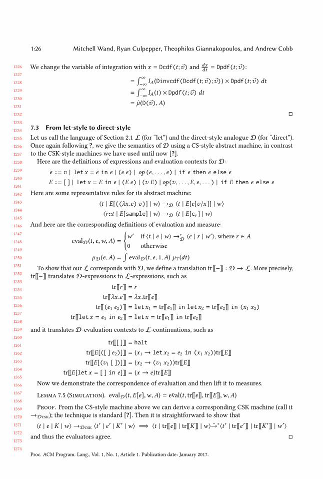
1226
1227
1228
1229
1230
1231
1232
1233
1234
1235
1236
1237
1238
1239
1240
1241
1242
1243
1244
1245
1246
1247
1248
1249
1250
1251
1252
1253
1254
1255
1256
1257
1258
1259
1260
1261
1262
1263
1264
1265
1266
1267
1268
1269
1270
1271
1272
1273
1274
1:26 Mitchell Wand, Ryan Culpepper, Theophilos Giannakopoulos, and Andrew Cobb
We change the variable of integration with x = Dcdf(t ; v) anddxdt = Dpdf(t ; v):
=∫ ∞−∞
IA (Dinvcdf(Dcdf(t ; v); v)) × Dpdf(t ; v) dt
=∫ ∞−∞
IA (t ) × Dpdf(t ; v) dt
= µ (D(v),A)
7.3 From let-style to direct-styleLet us call the language of Section 2.1 L (for “let”) and the direct-style analogue D (for “direct”).
Once again following ?, we give the semantics of D using a CS-style abstract machine, in contrast
to the CSK-style machines we have used until now [?].Here are the definitions of expressions and evaluation contexts for D:
e ::= v | letx = e in e | (e e) | op (e, . . . , e) | if e then e else e
E ::= [ ] | letx = E in e | (E e) | (v E) | op(v, . . . ,E, e, . . . ) | if E then e else e
Here are some representative rules for its abstract machine:
⟨t | E[((λx .e) v)] | w⟩ →D ⟨t | E[e[v/x]] | w⟩
⟨r ::t | E[sample] | w⟩ →D ⟨t | E[cr ] | w⟩
And here are the corresponding definitions of evaluation and measure:
evalD (t , e,w,A) =
w ′ if ⟨t | e | w⟩ →∗D⟨ϵ | r | w ′⟩, where r ∈ A
0 otherwise
µD (e,A) =∫evalD (t , e, 1,A) µT (dt )
To show that our L corresponds withD, we define a translation tr[[−]] : D → L. More precisely,
tr[[−]] translates D-expressions to L-expressions, such as
tr[[r ]] = r
tr[[λx .e]] = λx .tr[[e]]
tr[[(e1 e2)]] = letx1 = tr[[e1]] in letx2 = tr[[e2]] in (x1 x2)
tr[[letx = e1 in e2]] = letx = tr[[e1]] in tr[[e2]]
and it translates D-evaluation contexts to L-continuations, such as
tr[[[ ]]] = halt
tr[[E[([ ] e2)]]] = (x1 → letx2 = e2 in (x1 x2))tr[[E]]
tr[[E[(v1 [ ])]]] = (x2 → (v1 x2))tr[[E]]
tr[[E[letx = [ ] in e]]] = (x → e )tr[[E]]
Now we demonstrate the correspondence of evaluation and then lift it to measures.
Lemma 7.5 (Simulation). evalD (t ,E[e],w,A) = eval(t , tr[[e]], tr[[E]],w,A)
Proof. From the CS-style machine above we can derive a corresponding CSK machine (call it
→Dcsk); the technique is standard [?]. Then it is straightforward to show that
⟨t | e | K | w⟩ →Dcsk ⟨t′ | e ′ | K ′ | w⟩ =⇒ ⟨t | tr[[e]] | tr[[K]] | w⟩→∗⟨t ′ | tr[[e ′]] | tr[[K ′]] | w ′⟩
and thus the evaluators agree.
Proc. ACM Program. Lang., Vol. 1, No. 1, Article 1. Publication date: January 2017.
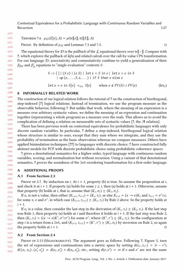
1275
1276
1277
1278
1279
1280
1281
1282
1283
1284
1285
1286
1287
1288
1289
1290
1291
1292
1293
1294
1295
1296
1297
1298
1299
1300
1301
1302
1303
1304
1305
1306
1307
1308
1309
1310
1311
1312
1313
1314
1315
1316
1317
1318
1319
1320
1321
1322
1323
Contextual Equivalence for a Probabilistic Language with Continuous Random Variables andRecursion 1:27
Theorem 7.6. µD (E[e],A) = µ (tr[[e]], tr[[E]],A)
Proof. By definition of µD and Lemmas 7.3 and 7.5.
The equational theory forD is the pullback of theL equational theory over tr[[−]]. Compare with
?, which explores the pullback of λβη and related calculi over the call-by-value CPS transformation.
For our language D, associativity and commutativity combine to yield a generalization of their
βflat and β ′Ω equations to “single-evaluation” contexts S :
S ::= [ ] | (S e) | (e S) | letx = S in e | letx = e in S| op (e, . . . , S, e, . . . ) | if S then e else e
letx = e in S[x] =ctx S[e] when x < FV (S ) ∪ FV (e ) (letS )
8 INFORMALLY RELATEDWORKThe construction of our logical relation follows the tutorial of ? on the construction of biorthogonal,
step-indexed [?] logical relations. Instead of termination, we use the program measure as the
observable behavior, following ?. But unlike that work, where the meaning of an expression is a
measure over arbitrary syntactic values, we define the meaning of an expression and continuation
together (representing a whole program) as a measure over the reals. This allows us to avoid the
complication of defining a relation on measurable sets of syntactic values [?, the A relation].
There has been previous work on contextual equivalence for probabilistic languages with only
discrete random variables. In particular, ? define a step-indexed, biorthogonal logical relation
whose structure is similar to ours, except that they sum where we integrate, and they use the
probability of termination as the basic observation whereas we compare measures. Others have
applied bisimulation techniques [??] to languages with discrete choice; ? have constructed fully
abstract models for PCF with discrete probabilistic choice using probabilistic coherence spaces.
? gives a denotational semantics for a higher-order, typed language with continuous random
variables, scoring, and normalization but without recursion. Using a variant of that denotational
semantics, ? proves the soundness of the let-reordering transformation for a first-order language.
A ADDITIONAL PROOFSA.1 From Section 2.3
Proof of 2.7. By induction on i . At i = 1, property (b) is true. So assume the proposition at i ,and check it at i + 1. If property (a) holds for some j ≤ i , then (a) holds at i + 1. Otherwise, assume
that property (b) holds at i , that is, assume that (Ki ,σi ) ⪰ (K1,σ1).If ei is not a value, then either (Ki+1,τi+1) = (Ki ,τi ), or else Ki+1 = (x → e )Ki and τi+1 = σ ′::τi
for some x , e and σ ′, in which case (Ki+1,τi+1) ⪰ (K1,τ1) by Rule 2 above. So the property holds at
i + 1.If ei is a value, then consider the last step in the derivation of (Ki ,τi ) ⪰ (K1,τ1). If the last step
was Rule 1, then property (a) holds at i and therefore it holds at i + 1. If the last step was Rule 2,
then (Ki ,τi ) = ((x → e )K ′,σ ′::τ ′) for some σ ′, where (K ′,τ ′) ⪰ (K1,τ1). So the configuration at
step i is a return from a let, and (Ki+1,τi+1) = (K ′,τ ′) ⪰ (K1,σ1) by inversion on Rule 2, so again
the property holds at i + 1.
A.2 From Section 2.4Proof of 2.13 (Measurability). The argument goes as follows. Following ?, Figure 5, turn
the set of expressions and continuations into a metric space by setting d (cr , cr ′ ) = |r − r ′ |;d ((e1 e2), (e
′1e ′2) = d (e1, e
′1) + d (e2, e
′2), etc., setting d (e, e ′) = ∞ if e and e ′ are not the same
Proc. ACM Program. Lang., Vol. 1, No. 1, Article 1. Publication date: January 2017.
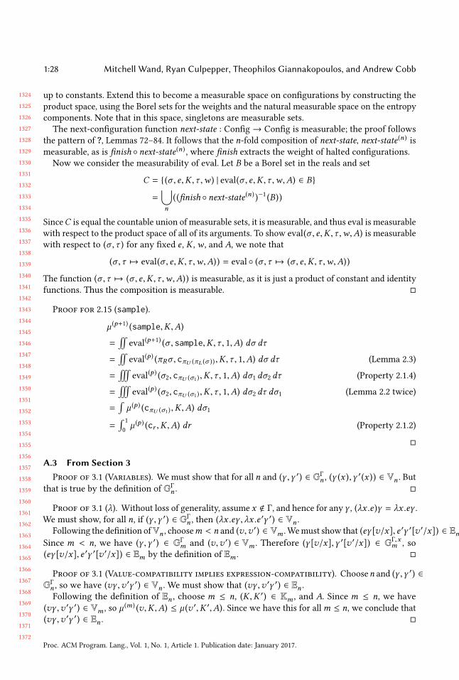
1324
1325
1326
1327
1328
1329
1330
1331
1332
1333
1334
1335
1336
1337
1338
1339
1340
1341
1342
1343
1344
1345
1346
1347
1348
1349
1350
1351
1352
1353
1354
1355
1356
1357
1358
1359
1360
1361
1362
1363
1364
1365
1366
1367
1368
1369
1370
1371
1372
1:28 Mitchell Wand, Ryan Culpepper, Theophilos Giannakopoulos, and Andrew Cobb
up to constants. Extend this to become a measurable space on configurations by constructing the
product space, using the Borel sets for the weights and the natural measurable space on the entropy
components. Note that in this space, singletons are measurable sets.
The next-configuration function next-state : Config→ Config is measurable; the proof follows
the pattern of ?, Lemmas 72–84. It follows that the n-fold composition of next-state, next-state(n) ismeasurable, as is finish next-state(n) , where finish extracts the weight of halted configurations.
Now we consider the measurability of eval. Let B be a Borel set in the reals and set
C = (σ , e,K ,τ ,w ) | eval(σ , e,K ,τ ,w,A) ∈ B
=⋃n
((finish next-state(n) )−1 (B))
SinceC is equal the countable union of measurable sets, it is measurable, and thus eval is measurable
with respect to the product space of all of its arguments. To show eval(σ , e,K ,τ ,w,A) is measurable
with respect to (σ ,τ ) for any fixed e , K ,w , and A, we note that
(σ ,τ 7→ eval(σ , e,K ,τ ,w,A)) = eval (σ ,τ 7→ (σ , e,K ,τ ,w,A))
The function (σ ,τ 7→ (σ , e,K ,τ ,w,A)) is measurable, as it is just a product of constant and identity
functions. Thus the composition is measurable.
Proof for 2.15 (sample).
µ (p+1) (sample,K ,A)
=!
eval(p+1) (σ , sample,K ,τ , 1,A) dσ dτ
=!
eval(p ) (πRσ , cπU (πL (σ )),K ,τ , 1,A) dσ dτ (Lemma 2.3)
=#
eval(p ) (σ2, cπU (σ1 ),K ,τ , 1,A) dσ1 dσ2 dτ (Property 2.1.4)
=#
eval(p ) (σ2, cπU (σ1 ),K ,τ , 1,A) dσ2 dτ dσ1 (Lemma 2.2 twice)
=∫µ (p ) (cπU (σ1 ),K ,A) dσ1
=∫
1
0µ (p ) (cr ,K ,A) dr (Property 2.1.2)
A.3 From Section 3Proof of 3.1 (Variables). We must show that for all n and (γ ,γ ′) ∈ GΓ
n , (γ (x ),γ′(x )) ∈ Vn . But
that is true by the definition of GΓn .
Proof of 3.1 (λ). Without loss of generality, assume x < Γ, and hence for any γ , (λx .e )γ = λx .eγ .We must show, for all n, if (γ ,γ ′) ∈ GΓ
n , then (λx .eγ , λx .e ′γ ′) ∈ Vn .Following the definition ofVn , choosem < n and (v,v ′) ∈ Vm .Wemust show that (eγ [v/x], e ′γ ′[v ′/x]) ∈ Em .
Since m < n, we have (γ ,γ ′) ∈ GΓm and (v,v ′) ∈ Vm . Therefore (γ [v/x],γ ′[v ′/x]) ∈ GΓ,x
m , so
(eγ [v/x], e ′γ ′[v ′/x]) ∈ Em by the definition of Em .
Proof of 3.1 (Value-compatibility implies expression-compatibility). Choosen and (γ ,γ ′) ∈GΓn , so we have (vγ ,v ′γ ′) ∈ Vn . We must show that (vγ ,v ′γ ′) ∈ En .Following the definition of En , choose m ≤ n, (K ,K ′) ∈ Km , and A. Since m ≤ n, we have
(vγ ,v ′γ ′) ∈ Vm , so µ (m) (v,K ,A) ≤ µ (v ′,K ′,A). Since we have this for allm ≤ n, we conclude that(vγ ,v ′γ ′) ∈ En .
Proc. ACM Program. Lang., Vol. 1, No. 1, Article 1. Publication date: January 2017.
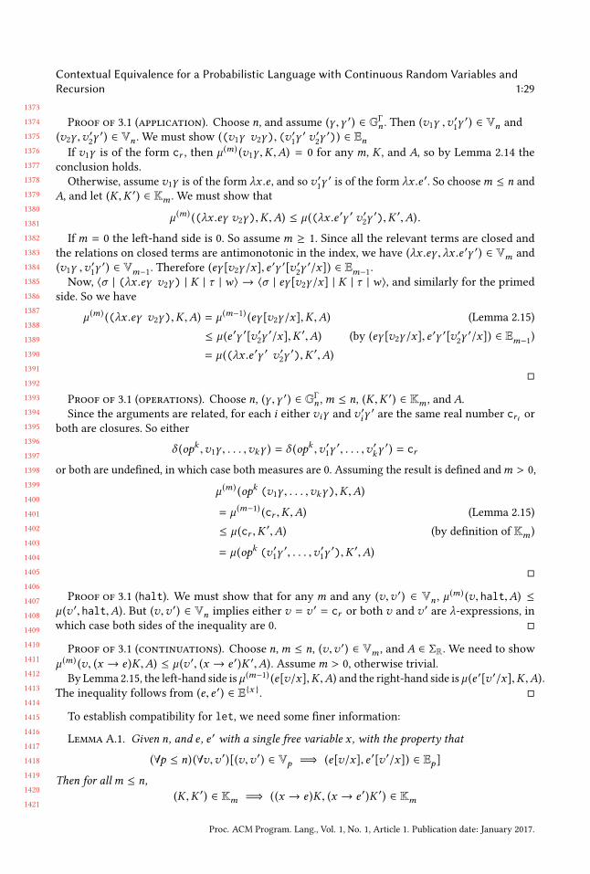
1373
1374
1375
1376
1377
1378
1379
1380
1381
1382
1383
1384
1385
1386
1387
1388
1389
1390
1391
1392
1393
1394
1395
1396
1397
1398
1399
1400
1401
1402
1403
1404
1405
1406
1407
1408
1409
1410
1411
1412
1413
1414
1415
1416
1417
1418
1419
1420
1421
Contextual Equivalence for a Probabilistic Language with Continuous Random Variables andRecursion 1:29
Proof of 3.1 (application). Choose n, and assume (γ ,γ ′) ∈ GΓn . Then (v1γ ,v
′1γ ′) ∈ Vn and
(v2γ ,v′2γ ′) ∈ Vn . We must show ((v1γ v2γ), (v
′1γ ′ v ′
2γ ′)) ∈ En
If v1γ is of the form cr , then µ (m) (v1γ ,K ,A) = 0 for any m, K , and A, so by Lemma 2.14 the
conclusion holds.
Otherwise, assume v1γ is of the form λx .e , and so v ′1γ ′ is of the form λx .e ′. So choosem ≤ n and
A, and let (K ,K ′) ∈ Km . We must show that
µ (m) ((λx .eγ v2γ),K ,A) ≤ µ ((λx .e ′γ ′ v ′2γ ′),K ′,A).
Ifm = 0 the left-hand side is 0. So assumem ≥ 1. Since all the relevant terms are closed and
the relations on closed terms are antimonotonic in the index, we have (λx .eγ , λx .e ′γ ′) ∈ Vm and
(v1γ ,v′1γ ′) ∈ Vm−1. Therefore (eγ [v2γ/x], e
′γ ′[v ′2γ ′/x]) ∈ Em−1.
Now, ⟨σ | (λx .eγ v2γ) | K | τ | w⟩ → ⟨σ | eγ [v2γ/x] | K | τ | w⟩, and similarly for the primed
side. So we have
µ (m) ((λx .eγ v2γ),K ,A) = µ (m−1) (eγ [v2γ/x],K ,A) (Lemma 2.15)
≤ µ (e ′γ ′[v ′2γ ′/x],K ′,A) (by (eγ [v2γ/x], e
′γ ′[v ′2γ ′/x]) ∈ Em−1)
= µ ((λx .e ′γ ′ v ′2γ ′),K ′,A)
Proof of 3.1 (operations). Choose n, (γ ,γ ′) ∈ GΓn ,m ≤ n, (K ,K ′) ∈ Km , and A.
Since the arguments are related, for each i either viγ and v ′iγ′are the same real number cri or
both are closures. So either
δ (opk ,v1γ , . . . ,vkγ ) = δ (opk ,v ′1γ ′, . . . ,v ′kγ
′) = cr
or both are undefined, in which case both measures are 0. Assuming the result is defined andm > 0,
µ (m) (opk (v1γ , . . . ,vkγ),K ,A)
= µ (m−1) (cr ,K ,A) (Lemma 2.15)
≤ µ (cr ,K′,A) (by definition of Km )
= µ (opk (v ′1γ ′, . . . ,v ′
1γ ′),K ′,A)
Proof of 3.1 (halt). We must show that for any m and any (v,v ′) ∈ Vn , µ(m) (v, halt,A) ≤
µ (v ′, halt,A). But (v,v ′) ∈ Vn implies either v = v ′ = cr or both v and v ′ are λ-expressions, inwhich case both sides of the inequality are 0.
Proof of 3.1 (continuations). Choose n,m ≤ n, (v,v ′) ∈ Vm , and A ∈ ΣR. We need to show
µ (m) (v, (x → e )K ,A) ≤ µ (v ′, (x → e ′)K ′,A). Assumem > 0, otherwise trivial.
By Lemma 2.15, the left-hand side is µ (m−1) (e[v/x],K ,A) and the right-hand side is µ (e ′[v ′/x],K ,A).The inequality follows from (e, e ′) ∈ Ex .
To establish compatibility for let, we need some finer information:
Lemma A.1. Given n, and e , e ′ with a single free variable x , with the property that
(∀p ≤ n) (∀v,v ′)[(v,v ′) ∈ Vp =⇒ (e[v/x], e ′[v ′/x]) ∈ Ep]
Then for allm ≤ n,(K ,K ′) ∈ Km =⇒ ((x → e )K , (x → e ′)K ′) ∈ Km
Proc. ACM Program. Lang., Vol. 1, No. 1, Article 1. Publication date: January 2017.
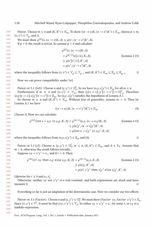
1422
1423
1424
1425
1426
1427
1428
1429
1430
1431
1432
1433
1434
1435
1436
1437
1438
1439
1440
1441
1442
1443
1444
1445
1446
1447
1448
1449
1450
1451
1452
1453
1454
1455
1456
1457
1458
1459
1460
1461
1462
1463
1464
1465
1466
1467
1468
1469
1470
1:30 Mitchell Wand, Ryan Culpepper, Theophilos Giannakopoulos, and Andrew Cobb
Proof. Choosem ≤ n and (K ,K ′) ∈ Km . To show ((x → e )K , (x → e ′)K ′) ∈ Km , choose p ≤ m,
(v,v ′) ∈ Vp , and A.
We must show µ (p ) (v, (x → e )K ,A) ≤ µ (v ′, (x → e ′)K ′,A).If p = 0, the result is trivial. So assume p > 0 and calculate:
µ (p ) (v, (x → e )K ,A)
= µ (p−1) (e[v/x],K ,A) (Lemma 2.15)
≤ µ (e ′[v ′/x],K ′,A)
= µ (v ′, (x → e ′)K ′,A)
where the inequality follows from (v,v ′) ∈ Vp ⊆ Vp−1 and (K ,K ′) ∈ Km ⊆ Kp ⊆ Kp−1.
Now we can prove compatibility under let.
Proof of 3.1 (let). Choose n and (γ ,γ ′) ∈ GΓn . So we have (e1γ , e
′1γ ′) ∈ Em for allm ≤ n.
Furthermore, if m ≤ n and (v,v ′) ∈ Vm , then (γ [x := v],γ ′[x := v ′]) ∈ GmΓ,x . Therefore(e2γ [x := v], e ′
2γ ′[x := v ′]) ∈ Em . So (e2γ , e
′2γ ′) satisfies the hypothesis of Lemma A.1.
So choose m ≤ n and (K ,K ′) ∈ Km . Without loss of generality, assume m > 0. Then by
Lemma A.1 we have
((x → eγ )K , (x → e ′γ ′)K ′) ∈ Km (3)
Choose A. Now we can calculate:
µ (m) (letx = e1γ in e2γ ,K ,A) = µ (m−1) (e1γ , (x → e2γ )K ,A) (Lemma 2.15)
≤ µ (e ′1γ ′, (x → e ′
2γ ′)K ′,A)
= µ (letx = e ′1γ ′ in e2γ
′,K ,A)
where the inequality follows from (e1γ , e′1γ ′) ∈ Em and (3).
Proof of 3.1 (if). Choose n, (γ ,γ ′) ∈ GΓn , m ≤ n, (K ,K ′) ∈ Km , and A ∈ ΣR. Assume that
m > 0, otherwise the result follows trivially.
Suppose vγ = v ′γ ′ = cr , and if r > 0. Then
µ (m) (if vγ then e1γ else e2γ ,K ,A) = µ (m−1) (e1γ ,K ,A) (Lemma 2.15)
≤ µ (e ′1γ ,K ′,A)
= µ (if v ′γ ′ then e ′1γ ′ else e ′
2γ ′,K ′,A)
Likewise for r ≤ 0 and e2, e′2.
Otherwise, neither vγ nor v ′γ ′ is a real constant, and both expressions are stuck and have
measure 0.
Everything so far is just an adaptation of the deterministic case. Now we consider our two effects.
Proof of 3.1 (factor). Choosen and (γ ,γ ′) ∈ GnΓ .Wemust show (factor vγ , factor v ′γ ′) ∈ En .
Since (v,v ′) ∈ VΓ, it must be that (vγ ,v ′γ ′) ∈ Vn . So either vγ = v ′γ ′ = cr for some r , or vγ is a
lambda-expression.
Proc. ACM Program. Lang., Vol. 1, No. 1, Article 1. Publication date: January 2017.
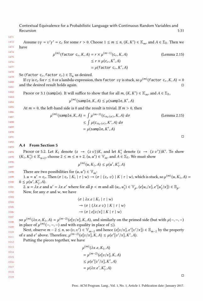
1471
1472
1473
1474
1475
1476
1477
1478
1479
1480
1481
1482
1483
1484
1485
1486
1487
1488
1489
1490
1491
1492
1493
1494
1495
1496
1497
1498
1499
1500
1501
1502
1503
1504
1505
1506
1507
1508
1509
1510
1511
1512
1513
1514
1515
1516
1517
1518
1519
Contextual Equivalence for a Probabilistic Language with Continuous Random Variables andRecursion 1:31
Assume vγ = v ′γ ′ = cr for some r > 0. Choose 1 ≤ m ≤ n, (K ,K ′) ∈ Km , and A ∈ ΣR. Then we
have
µ (m) (factor cr ,K ,A) = r × µ(m−1) (cr ,K ,A) (Lemma 2.15)
≤ r × µ (cr ,K′,A)
= µ (factor cr ,K′,A)
So (factor cr , factor cr ) ∈ En as desired.
Ifvγ is cr for r ≤ 0 or a lambda-expression, then factor vγ is stuck, so µ (m) (factor cr ,K ,A) = 0
and the desired result holds again.
Proof of 3.1 (sample). It will suffice to show that for allm, (K ,K ′) ∈ Km , and A ∈ ΣR,
µ (m) (sample,K ,A) ≤ µ (sample,K ′,A)
Atm = 0, the left-hand side is 0 and the result is trivial. Ifm > 0, then
µ (m) (sample,K ,A) =∫µ (m−1) (cπU (σ ),K ,A) dσ (Lemma 2.15)
≤∫µ (cπU (σ ),K
′,A) dσ
= µ (sample,K ′,A)
A.4 From Section 5Proof of 5.2. Let K1 denote (z → (z v))K , and let K ′
1denote (z → (z v ′))K ′. To show
(K1,K′1) ∈ Kn+2, choose 2 ≤ m ≤ n + 2, (u,u ′) ∈ Vm , and A ∈ ΣR. We must show
µ (m) (u,K1,A) ≤ µ (u ′,K ′1,A)
There are two possibilities for (u,u ′) ∈ Vm :1.u = u ′ = cr . Then ⟨σ | cr | K1 | τ | w⟩ → ⟨σ | (cr v) | K | τ | w⟩, which is stuck, so µ
(m) (u,K1,A) =0 ≤ µ (u ′,K ′
1,A).
2. u = λx .e and u ′ = λx .e ′ where for all p < m and all (u1,u′1) ∈ Vp , (e[u1/x], e
′[u ′
1/x]) ∈ Ep .
Now, for any σ andw , we have
⟨σ | λx .e | K1 | τ | w⟩
→ ⟨σ | (λx .e v) | K | τ | w⟩
→ ⟨σ | e[v/x] | K | τ | w⟩
so µ (m) (λx .e,K1,A) = µ (m−2) (e[v/x],K ,A), and similarly on the primed side (but with µ (−,−,−)in place of µ (m) (−,−,−) and with equality in place of ≤).
Next, observem − 2 ≤ n, so (v,v ′) ∈ Vm−2 and hence (e[v/x], e ′[v ′/x]) ∈ Em−2 by the property
of e and e ′ above. Therefore, µ (m−2) (e[v/x],K ,A) ≤ µ (e ′[v ′/x],K ′,A).Putting the pieces together, we have
µ (m) (λx .e,K1,A)
= µ (m−2) (e[v/x],K ,A)
≤ µ (e ′[v ′/x],K ′,A)
= µ (λx .e ′,K ′1,A)
Proc. ACM Program. Lang., Vol. 1, No. 1, Article 1. Publication date: January 2017.
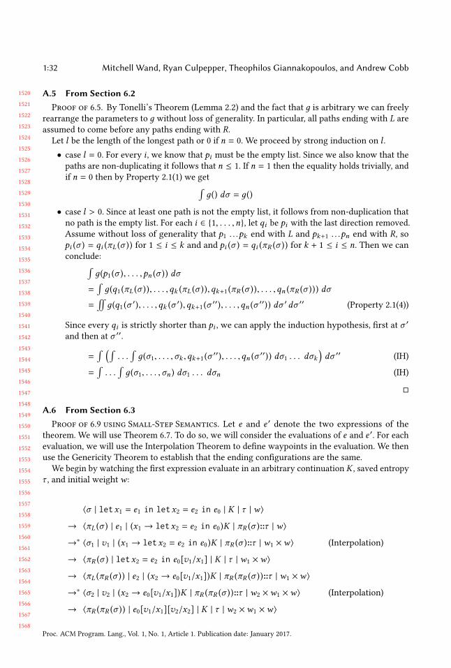
1520
1521
1522
1523
1524
1525
1526
1527
1528
1529
1530
1531
1532
1533
1534
1535
1536
1537
1538
1539
1540
1541
1542
1543
1544
1545
1546
1547
1548
1549
1550
1551
1552
1553
1554
1555
1556
1557
1558
1559
1560
1561
1562
1563
1564
1565
1566
1567
1568
1:32 Mitchell Wand, Ryan Culpepper, Theophilos Giannakopoulos, and Andrew Cobb
A.5 From Section 6.2Proof of 6.5. By Tonelli’s Theorem (Lemma 2.2) and the fact that д is arbitrary we can freely
rearrange the parameters to д without loss of generality. In particular, all paths ending with L are
assumed to come before any paths ending with R.Let l be the length of the longest path or 0 if n = 0. We proceed by strong induction on l .
• case l = 0. For every i , we know that pi must be the empty list. Since we also know that the
paths are non-duplicating it follows that n ≤ 1. If n = 1 then the equality holds trivially, and
if n = 0 then by Property 2.1(1) we get∫д() dσ = д()
• case l > 0. Since at least one path is not the empty list, it follows from non-duplication that
no path is the empty list. For each i ∈ 1, . . . ,n, let qi be pi with the last direction removed.
Assume without loss of generality that p1 . . .pk end with L and pk+1 . . .pn end with R, sopi (σ ) = qi (πL (σ )) for 1 ≤ i ≤ k and and pi (σ ) = qi (πR (σ )) for k + 1 ≤ i ≤ n. Then we can
conclude:∫д(p1 (σ ), . . . ,pn (σ )) dσ
=∫д(q1 (πL (σ )), . . . ,qk (πL (σ )),qk+1 (πR (σ )), . . . ,qn (πR (σ ))) dσ
=!
д(q1 (σ′), . . . ,qk (σ
′),qk+1 (σ′′), . . . ,qn (σ
′′)) dσ ′dσ ′′ (Property 2.1(4))
Since every qi is strictly shorter than pi , we can apply the induction hypothesis, first at σ ′
and then at σ ′′.
=∫ (∫
. . .∫д(σ1, . . . ,σk ,qk+1 (σ
′′), . . . ,qn (σ′′)) dσ1 . . . dσk
)dσ ′′ (IH)
=∫. . .∫д(σ1, . . . ,σn ) dσ1 . . . dσn (IH)
A.6 From Section 6.3Proof of 6.9 using Small-Step Semantics. Let e and e ′ denote the two expressions of the
theorem. We will use Theorem 6.7. To do so, we will consider the evaluations of e and e ′. For eachevaluation, we will use the Interpolation Theorem to define waypoints in the evaluation. We then
use the Genericity Theorem to establish that the ending configurations are the same.
We begin by watching the first expression evaluate in an arbitrary continuation K , saved entropyτ , and initial weightw :
⟨σ | letx1 = e1 in letx2 = e2 in e0 | K | τ | w⟩
→ ⟨πL (σ ) | e1 | (x1 → letx2 = e2 in e0)K | πR (σ )::τ | w⟩
→∗ ⟨σ1 | v1 | (x1 → letx2 = e2 in e0)K | πR (σ )::τ | w1 ×w⟩ (Interpolation)
→ ⟨πR (σ ) | letx2 = e2 in e0[v1/x1] | K | τ | w1 ×w⟩
→ ⟨πL (πR (σ )) | e2 | (x2 → e0[v1/x1])K | πR (πR (σ ))::τ | w1 ×w⟩
→∗ ⟨σ2 | v2 | (x2 → e0[v1/x1])K | πR (πR (σ ))::τ | w2 ×w1 ×w⟩ (Interpolation)
→ ⟨πR (πR (σ )) | e0[v1/x1][v2/x2] | K | τ | w2 ×w1 ×w⟩
Proc. ACM Program. Lang., Vol. 1, No. 1, Article 1. Publication date: January 2017.

1569
1570
1571
1572
1573
1574
1575
1576
1577
1578
1579
1580
1581
1582
1583
1584
1585
1586
1587
1588
1589
1590
1591
1592
1593
1594
1595
1596
1597
1598
1599
1600
1601
1602
1603
1604
1605
1606
1607
1608
1609
1610
1611
1612
1613
1614
1615
1616
1617
Contextual Equivalence for a Probabilistic Language with Continuous Random Variables andRecursion 1:33
Next, we outline the analogous computation with the second expression e ′, starting in a different
entropy σ ′, but with the same continuation K , saved entropy τ , and weightw . We proceed under
the assumption that e ′ reduces to a value; we will validate this assumption later.
⟨σ ′ | letx2 = e2 in letx1 = e1 in e0 | K | τ | w⟩
→ ⟨πL (σ′) | e2 | (x2 → letx1 = e1 in e0)K | πR (σ
′)::τ | w⟩
→∗ ⟨σ ′2| v ′
2| (x2 → letx1 = e1 in e0)K | πR (σ
′)::τ | w ′2×w⟩ (Interpolation)
→ ⟨πR (σ′) | letx1 = e1 in e0[v
′2/x2] | K | τ | w
′2×w⟩
→ ⟨πL (πR (σ′)) | e1 | (x1 → e0[v
′2/x2])K | πR (πR (σ
′))::τ | w ′2×w⟩
→∗ ⟨σ ′1| v ′
1| (x1 → e0[v
′2/x2])K | πR (πR (σ
′))::τ | w ′1×w ′
2×w⟩ (Interpolation)
→ ⟨πR (πR (σ′)) | e0[v
′2/x2][v
′1/x1] | K | τ | w
′1×w ′
2×w⟩
To get these computations to agree, we choose σ ′ so that the entropies for e1, e2 and the substi-
tution instances of e0 are the same in both calculations. So we choose σ ′ such that
πL (πR (σ′)) = πL (σ ) (entropy for e1)
πL (σ′) = πL (πR (σ )) (entropy for e2)
πR (πR (σ′)) = πR (πR (σ )) (entropy for e0)
This can be accomplished by using ϕc from Section 6.2; we set
σ ′ = ϕc (σ ) = πL (πR (σ ))::(πL (σ )::πR (πR (σ )))
Applying the genericity theorem at e1 we conclude that that e1 reduces to a value at entropy
πL (πRσ′)) = πL (σ ) and continuation (x1 → e0[v
′2/x2])K , that v1 = v
′1, and thatw1 = w
′1. Similarly
applying the genericity theorem at e2 we conclude that e2 reduces to a value v ′2= v2 andw2 = w
′2.
So the two calculations culminate in identical configurations.
So we conclude that
eval(σ , e,K ,τ , 1,A) = eval(ϕc (σ ), e′,K ,τ , 1,A)
ϕc is a non-duplicating FSF, so it is measure-preserving by Theorem 6.6. Then by Theorem 6.7,
(e, e ′) ∈ CTX. The converse holds by symmetry.
B EXAMPLE TRANSFORMATION SKETCHThis section gives a sketch of the transformation of the linear regression example from Section 1.
Here is the initial program:
A = normal(0, 10)B = normal(0, 10)f(x) = A*x + Bfactor normalpdf(f(2) - 2.4; 0, 1)factor normalpdf(f(3) - 2.7; 0, 1)factor normalpdf(f(4) - 3.0; 0, 1)
Our first goal is to reshape the program to expose the conjugacy relationship between B’s priorand the observations. Specifically, we need the observations to be expressed with B as the mean.
The following steps perform the reshaping.
Inline f using letv :
Proc. ACM Program. Lang., Vol. 1, No. 1, Article 1. Publication date: January 2017.
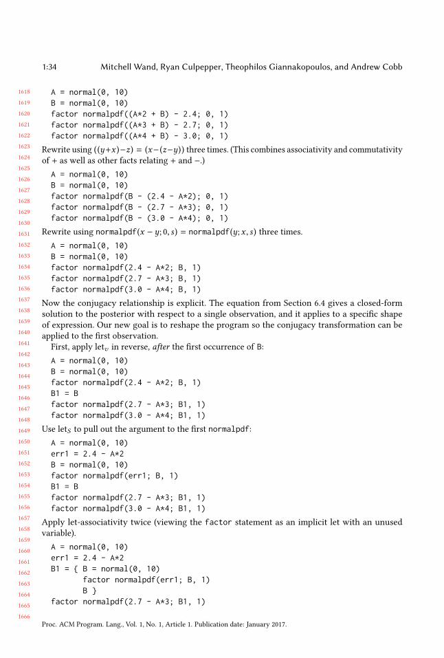
1618
1619
1620
1621
1622
1623
1624
1625
1626
1627
1628
1629
1630
1631
1632
1633
1634
1635
1636
1637
1638
1639
1640
1641
1642
1643
1644
1645
1646
1647
1648
1649
1650
1651
1652
1653
1654
1655
1656
1657
1658
1659
1660
1661
1662
1663
1664
1665
1666
1:34 Mitchell Wand, Ryan Culpepper, Theophilos Giannakopoulos, and Andrew Cobb
A = normal(0, 10)B = normal(0, 10)factor normalpdf((A*2 + B) - 2.4; 0, 1)factor normalpdf((A*3 + B) - 2.7; 0, 1)factor normalpdf((A*4 + B) - 3.0; 0, 1)
Rewrite using ((y+x )−z) = (x−(z−y)) three times. (This combines associativity and commutativity
of + as well as other facts relating + and −.)
A = normal(0, 10)B = normal(0, 10)factor normalpdf(B - (2.4 - A*2); 0, 1)factor normalpdf(B - (2.7 - A*3); 0, 1)factor normalpdf(B - (3.0 - A*4); 0, 1)
Rewrite using normalpdf(x − y; 0, s ) = normalpdf(y;x , s ) three times.
A = normal(0, 10)B = normal(0, 10)factor normalpdf(2.4 - A*2; B, 1)factor normalpdf(2.7 - A*3; B, 1)factor normalpdf(3.0 - A*4; B, 1)
Now the conjugacy relationship is explicit. The equation from Section 6.4 gives a closed-form
solution to the posterior with respect to a single observation, and it applies to a specific shape
of expression. Our new goal is to reshape the program so the conjugacy transformation can be
applied to the first observation.
First, apply letv in reverse, after the first occurrence of B:
A = normal(0, 10)B = normal(0, 10)factor normalpdf(2.4 - A*2; B, 1)B1 = Bfactor normalpdf(2.7 - A*3; B1, 1)factor normalpdf(3.0 - A*4; B1, 1)
Use letS to pull out the argument to the first normalpdf:
A = normal(0, 10)err1 = 2.4 - A*2B = normal(0, 10)factor normalpdf(err1; B, 1)B1 = Bfactor normalpdf(2.7 - A*3; B1, 1)factor normalpdf(3.0 - A*4; B1, 1)
Apply let-associativity twice (viewing the factor statement as an implicit let with an unused
variable).
A = normal(0, 10)err1 = 2.4 - A*2B1 = B = normal(0, 10)
factor normalpdf(err1; B, 1)B
factor normalpdf(2.7 - A*3; B1, 1)
Proc. ACM Program. Lang., Vol. 1, No. 1, Article 1. Publication date: January 2017.
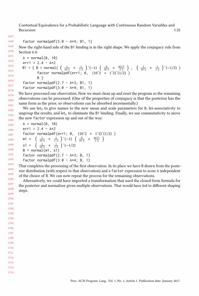
1667
1668
1669
1670
1671
1672
1673
1674
1675
1676
1677
1678
1679
1680
1681
1682
1683
1684
1685
1686
1687
1688
1689
1690
1691
1692
1693
1694
1695
1696
1697
1698
1699
1700
1701
1702
1703
1704
1705
1706
1707
1708
1709
1710
1711
1712
1713
1714
1715
Contextual Equivalence for a Probabilistic Language with Continuous Random Variables andRecursion 1:35
factor normalpdf(3.0 - A*4; B1, 1)
Now the right-hand side of the B1 binding is in the right shape. We apply the conjugacy rule from
Section 6.4:
A = normal(0, 10)err1 = 2.4 - A*2B1 = B = normal(
(1
10ˆ2+ 1
1ˆ2
)ˆ(−1)
(0
10ˆ2+ err1
1ˆ2
),(
1
10ˆ2+ 1
1ˆ2
)ˆ(−1/2) )
factor normalpdf(err1; 0, (10ˆ2 + 1ˆ2)ˆ(1/2) )B
factor normalpdf(2.7 - A*3; B1, 1)factor normalpdf(3.0 - A*4; B1, 1)
We have processed one observation. Now we must clean up and reset the program so the remaining
observations can be processed. (One of the properties of conjugacy is that the posterior has the
same form as the prior, so observations can be absorbed incrementally.)
We use letS to give names to the new mean and scale parameters for B, let-associativity to
ungroup the results, and letv to eliminate the B1 binding. Finally, we use commutativity to move
the new factor expression up and out of the way.
A = normal(0, 10)err1 = 2.4 - A*2factor normalpdf(err1; 0, (10ˆ2 + 1ˆ2)ˆ(1/2) )
m1 =(
1
10ˆ2+ 1
1ˆ2
)ˆ(−1)
(0
10ˆ2+ err1
1ˆ2
)s1 =
(1
10ˆ2+ 1
1ˆ2
)ˆ(−1/2)
B = normal(m1, s1)factor normalpdf(2.7 - A*3; B, 1)factor normalpdf(3.0 - A*4; B, 1)
That completes the processing of the first observation. In its place we have B drawn from the poste-
rior distribution (with respect to that observation) and a factor expression to score A independent
of the choice of B. We can now repeat the process for the remaining observations.
Alternatively, we could have imported a transformation that used the closed-form formula for
the posterior and normalizer given multiple observations. That would have led to different shaping
steps.
Proc. ACM Program. Lang., Vol. 1, No. 1, Article 1. Publication date: January 2017.


![SlimShot: Probabilistic Inference for Web-Scale Knowledge ...suciu/file41_paper.pdf · Equivalence of queries Q Q0is NP-complete [31], and, by duality, equivalence of constraints](https://img.dokumen.tips/doc/110x75/5f649ede1eca732a4f62cf14/slimshot-probabilistic-inference-for-web-scale-knowledge-suciufile41paperpdf.jpg)