A PROBABILISTIC NETWORK FORENSIC MODEL FOR

EVIDENCE ANALYSIS

Changwei Liu#1

, Anoop Singhal*2

, Duminda Wijesekera#,*3

#Department of Computer Science, George Mason University, Fairfax VA 22030 USA

1cliu6@gmu.edu,

3dwijesek@gmu.edu

*National Institute of Standards and Technology, Gaithersburg MD 20899 USA

2anoop.singhal@nist.gov

Abstract: Modern-day attackers tend to use sophisticated multi-stage/multi-host attack

techniques and anti-forensic tools to cover their attack traces. Due to the current limitations of

intrusion detection systems (IDS) and forensic analysis tools, evidence can be false positives or

missing. Additionally, because of the large number of security events, finding an attack pattern

may become like finding a needle in a haystack. Consequently, reconstructing attack scenarios

that can hold the attackers accountable for their activities becomes a challenge.

This paper describes a probabilistic model that applies Bayesian Network to constructed

evidence graphs, systematically addressing how to solve some of the above problem by detecting

false positives, analyzing the reasons of missing evidence and computing the posterior

probabilities and false positive rates of an attack scenario constructed by discovered evidence.

We have also developed an accompanying software tool for network forensic analysis. Our

system is based on Prolog and use known vulnerability databases and an anti-forensics database

that is similar to the NIST National Vulnerability Database (NVD). Our experimental results

show that such a system is useful for constructing the most likely attack scenario and managing

errors for network forensic analysis.

Keywords: Network forensics, Digital evidence, Logical evidence graphs, Bayesian Network

1

1. INTRODUCTION

Digital forensics investigators use evidence and contextual facts to formulate attack

hypotheses, and assess the probability that the facts support or refute hypotheses on network

attacks [7]. However, due to the limitations of forensics tools and experts’ knowledge,

formalizing a hypothesis and using quantitative measures to support the hypothesis on a multi-

step, multi-host attack launched toward an enterprise network becomes a challenge. As a

solution, we designed a method and developed a software tool to partially automate the process

of constructing quantitatively supportable attack scenarios by using the available evidence. We

show its applicability using a case study of an attack.

Our method uses a Bayesian Network (BN) to estimate the likelihood and false positive

rates of potential attack scenarios that fit discovered evidence. Although BNs have been used for

digital evidence modeling [5,6,7,12], to the best of our knowledge these publications construct

BNs in an ad hoc manner. In this paper, we show how our method automates the process of

organizing evidence in a graphical structure (that we call a logical evidence graph) and apply

Bayesian analysis to the entire graph. By doing so, our system can: (1) provide us attack

scenarios with acceptable false positive rates, and (2) dynamically update the joint posterior

probability and false positive rate of an attack path when new item of evidence for the attack

path is presented.

The rest of this paper is organized as follows. Section 2 provides background and related

work. Section 3 describes logical evidence graphs. Section 4 describes our probabilistic analysis.

Section 5 describes a case study. Section 6 concludes the paper.

2. BACKGROUND AND RELATED WORK

2

BNs have been used to facilitate the expression of opinions regarding legal

determinations on the credibility and relative weight of non-digital evidence [5, 6, 7, 8, 12].

Many researchers of criminal forensics use BNs to model dependencies between hypotheses and

evidence taken from crime scenes and use these models to update the belief probability of newly

found evidence given the previous ones [5, 6, 8, 10,11, 12]. In digital forensics, researchers also

have used BNs to reason about evidence in order to quantify the strengths in supporting the

reliability and traceability of corresponding hypotheses [7]. However, these BNs were custom-

built without using a uniform model. Given the evidence, tools that directly support

automatically building a BN and estimating belief probabilities as well as corresponding

potential error rate have been minimal.

Our system presented in this paper is based on a Prolog-based reasoning system MulVAL

[13,14] using known vulnerability databases and an anti-forensics database that we plan to

extend to a standardized database like the NIST National Vulnerability Database (NVD).

3. LOGICAL EVIDENCE GRAPHS

This section defines logical evidence graphs and shows how we design rules to correlate

available evidence to attack scenarios. Because we use reasoning to link observed attack events

and collected evidence, we call such an evidence graph a logical evidence graph.

Definition 1 (Logical Evidence Graph- LEG): A LEG=(Nr,Nf,Nc,E,L,G) is said to be a

logical evidence graph (LEG), where Nf, Nr and Nc are three sets of disjoint nodes in the graph

(they are called fact, rule, and consequence fact nodes respectively), E ⊆ ((Nf∪Nc)×Nr)∪( Nr

×Nc) ), and L is the mapping from a node to its labels. G⊆ Nc are the observed attack events.

Every rule node has a consequence fact node as its single child and one or more fact or

consequence fact nodes from prior attack steps as its parents. Node labels consist of

3

instantiations of rules or sets of predicates specified as follows:

1. A node in Nf is an instantiation of predicates that codify system state including access

privileges, network topology consisting interconnectivity information, or known vulnerabilities

associated with host computers in the system. We use the following predicates:

a. “hasAccount(_principal, _host, _account)”, “canAccessFile(_host, _user, _access,

_path)” and etc. to model access privileges.

b. “attackerLocated(_host)” and “hacl(_src, _dst, _prot, _port)” to model network topology,

namely, the attacker’s location and network reachability information.

c. “vulExists(_host, _vulID, _program)” and “vulProperty(_vulID, _range, _consequence)”

to model vulnerabilities exhibited by nodes.

2. A node in Nc represents the predicate that codifies the post attack state as the consequence of

an attack step. We use predicates “execCode(_host,_user)” and “netAccess(_machine,_protocol,

_port)” to model the attacker’s capability after an attack step. Valid instantiations of these

predicates after an attack will update valid instantiation of the predicates listed in (1).

3. A node in Nr consists of a single rule in the form pp1p2,.,pn, where p as the child node of

Nr is an instantiation of predicates from Nc , and all pi for i{1,…n} as the parent nodes of Nr are

the collection of all predicate instantiations of Nf from the current step and Nc from prior attack

steps.

Figure 1 is an example LEG (the notation of all nodes is in the Table 1), where fact, rule

and consequence fact nodes are represented as boxes, ellipses, and diamonds respectively.

Consequence fact nodes (Node 1 and 3) codify attack status obtainable from event logs or other

forensic tools recording the post-conditions of attack steps. Facts (Node 5, 6, 7 and 8) include

software vulnerability (Node 8) extracted from forensic tools by analyzing captured evidence,

4

computer configuration (Node 7) and network topology of a network (Node 5, 6). Rule nodes

(node 4 and 2) represent specific rules that change the attack status using attack steps. These

rules are created from expert knowledge, which are used to link chains of evidence as

consequences of attack steps. Linking the chain of evidence by using a rule forms an

investigator’s hypothesis of an attack step given the evidence.

Figure 1: An Example Logical Evidence Graph

Table 1: The notation of nodes in Figure 1

Node Notation Resource

1 execCode(workStation1,user) Evidence obtained from event

log

2 THROUGH 3 (remote exploit of a server program) Rule 1 (hypothesis 1)

3 netAccess(workStation1,tcp,4040) Evidence obtained from event

log

4 THROUGH 8 (direct network access) Rule 2 (hypothesis 2)

5 hacl(internet,workStation1,tcp,4040) Network setup

6 attackerLocated(internet) Evidence obtained from log

7 networkServiceInfo(workStation1,httpd,tcp,4040,user) Computer setup

8 vulExists(workStation1,'CVE-2009-1918',

httpd,remoteExploit,privEscalation)

Exploited vulnerability obtained

from IDS Alert

Figure 2 lists the two rules (Rule 1 and Rule 2 in Table 1) between Line 9 and Line 17.

Rules use the Prolog notation “: -“ to separate the head (consequence) and the body (facts). In

5

Figure 2, lines 1 to 8 identify fact and consequence predicates of the two rules. Rule 1 between

lines 9 to 12 in Figure 2 represents an attack step that states: if (1) the attacker is located in a

“Zone” such as “internet” (Line 10- attackerLocated(Zone)), and (2) a host computer “H” can be

accessed from the “Zone” by using “Protocol” at “Port”(Line 11-hacl(Zone, H, Protocol, Port)),

then (3) the host “H” can be accessed from the “Zone” by using “Protocol” at “Port” (Line 9-

netAccess(H, Protocol, Port)) via (4) “direct network access” (Line 12--the description of the

rule). Rule 2 between lines 13 to 17 states: if (1) a host has software vulnerability that can be

remotely exploited (Line 14- vulExists(H, _, Software, remoteExploit, privEscalation) ), and (2)

the host can be reached by using “Protocol” at “Port” with the privilege “Perm” ( Line 15-

networkServiceInfo(H, Software, Protocol, Port, Perm) ), and (3) the attacker can access host by

“Protocol” at “Port” (Line 16-netAccess(H, Protocol, Port) ), then (4) the attacker can remotely

exploit the host “H” and obtain the privilege “Perm”(Line 13- execCode(H, Perm) ) via (5)

“'remote exploit of a server program” technique (Line 17—the description of the rule).

//Rule Head--post attack status as derived fact obtained from forensic analysis on evidence

1. Consequence: execCode(_host, _user).

2. Consequence: netAccess(_machine,_protocol,_port).

// Rule body--access priviledge

3. Fact: hacl(_src, _dst, _prot, _port).

//Rule body--software vulnerability obtained from forensic tool

4. Fact: vulExists(_host, _vulID, _program).

5. Fact: vulProperty(_vulID, _range, _consequence).

//Rule body--network topology

6. Fact: hacl(_src, _dst, _prot, _port).

7. Fact: attackerLocated(_host).

//Rule body--computer configuration

8. Fact: hasAccount(_principal, _host, _account).

Rule 1:

9. (netAccess(H, Protocol, Port) :-

6

10. attackerLocated(Zone),

11. hacl(Zone, H, Protocol, Port)),

12. rule_desc('direct network access', 1.0).

Rule 2:

13. (execCode(H, Perm) :-

14. vulExists(H, _, Software, remoteExploit, privEscalation),

15. networkServiceInfo(H, Software, Protocol, Port, Perm),

16. netAccess(H, Protocol, Port)),

17. rule_desc('remote exploit of a server program', 1.0).

Figure 2: The Example Rules Representing Attack Techniques

4. COMPUTING PROBABILITIES USING BAYESIAN INFERENCE

Bayesian networks [3] use a directed acyclic graph (DAG) where nodes represent random

variables (RVs) (events or evidence in our case) and arcs model direct dependencies between

RVs. Every node has a table (CPT) that provides the conditional probability of the node’s

variable given the combination of its parent variables’ states.

Definition 2 (Bayesian Network): Suppose random variables X1,X2,...,Xn are n random

variables connected in a DAG, the joint probability distribution of X1,X2,...,Xn can be computed

by using the Bayesian formula P(X1,X2,…,Xn) = ∏ 〖𝑃(𝑋𝑗)|𝑃𝑎𝑟𝑒𝑛𝑡(𝑋𝑗)〗𝑛𝑗=1

, in which

parent(Xj)= {Xi | arc (ij) is in the graph}.

Figure 3: Causal View of Evidence

A BN can model and visualize dependencies between the hypothesis and evidence

to calculate the revised probability when any evidence is presented [11]. Dependency probability

of a hypothesis H about created scenarios on discovered evidence E can be modeled as shown in

7

Figure 3. Hence, Bayes’ theorem can be used to update an investigator’s belief about a

hypothesis H when the evidence E is observed, using Equation (1):

P(H|E)=𝑃(𝐻)𝑃(𝐸|𝐻)

𝑃(𝐸) =

𝑃(𝐻)𝑃(𝐸|𝐻)

P(E|H)∗P(H) + P(E|not H)∗P(not H) (1)

In Equation (1), P(H|E) is the posterior probability of an investigator’s belief on

hypothesis H given the evidence E. P(E|H) needs to come from experts’ knowledge, referred to

as the likelihood function that assesses the probability of evidence assuming the truth of H. P(H)

is the prior probability of H when the evidence has not been discovered and P(E) = P(E|H)*P(H)

+ P(E| H)*P( H) is the probability of the evidence irrespective of the experts’ knowledge

about H, referred to as a normalizing constant [1,7].

4.1 Calculating P(H|E) in a Logical Evidence Graph

An LEG consists of a serial application of attack steps, which can be mapped to a BN as

follows: (1) “Nc” as the child of the corresponding “Nr” shows that an attack step happened; (2)

“Nr” is the hypothesis of the attack step, denoted by “H”; (3) “Nf” from the current attack step

and “Nc′ ” from last attack step as the parents of “Nr” are attack evidence, showing the exploited

vulnerability and the attack privilege the attacker used to launch the attack step; (4) “Nc”

propagates the dependency between the current attack step and the subsequent one( “Nc” is also

the pre-condition of the subsequent attack step).

4.1.1. Computing P(H|E) for a Consequence Fact Node

Equation (1) can be used to compute P(H|E) for a consequence fact node of a single

attack step when the prior attack step has not been considered where the rule node provides the

hypothesis H, both the fact node “Nf” and the consequence node from a prior attack step “Nc′”

provide evidence E. Because a hypothesis H is a rule node “Nr”, Bayes’ theorem implies

Equation (2):

Comment [CL1]: Chang not to in LaTex

8

P(H|E)=P(Nr|E)= 𝑃(Nr)𝑃(E|Nr)

𝑃(E) (2)

The fact nodes from current attack step and the consequence fact node from a prior attack

step are independent to each other. They provide the body of the rule, deriving the consequence

fact node for the current attack step as the head of the rule. Consequently, their logical

conjunction provides the conditions that are used to arrive at the conclusion of rule. Accordingly,

if a rule node has “k” many parents Np1, Np2, …, Npk that are independent, P(E)=

P(Np1,Np2,…,Npk) = P(Np1∩Np2∩…∩Npk)=P(Np1).P(Np2)….P(Npk)( ∩ means “and”). Due to the

independence, given the rule Nr ， P(E|Nr)= P(Np1, Np2,..,

Npk|Nr)=P(Np1|Nr).P(Np2|Nr)…P(Npk|Nr). Hence, by applying Equation (2) where H is Nr and E is

Np1∩Np2∩…∩Npk, we get Equation (3) to compute P(H|E) for a consequence fact node.

P(H|E) =P(Nr| Np1,Np2 ,…,Npk) =𝑃(Nr)P(Np1 |Nr).P(Np2 |Nr)… P(Npk |Nr)

𝑃(Np1)𝑃(Np2)…𝑃(Npk) (3)

However, because P(E|Nr) is forensic investigators’ subjective judgment, it would be

difficult for human experts to assign P(Np1 |Nr), P(Np2 |Nr) … P(Npk |Nr) separately. We allow the

investigators’ discretion of using Equations (2) to consider P(E|Nr) directly.

4.1.2. Computing P(H|E) for the Entire Logical Evidence Graph

Now we show how to compute P(H|E) for the entire LEG composing of attack paths. Any

chosen attack path in a LEG consists of a serial application of attack steps. Suppose Si（i＝1 to

n) represents the ith

attack step in an attack path. Because an attack step only depends on its direct

parent attack step, but is independent from all other ancestor attack steps in the attack path, by

applying Definition (2), we get Equation (4) as follows.

P(H|E) = P(H1,H2…Hn|E1,E2,E3…En) = P(S1)P(S2|S1)….P(Sn|Sn-1) (4)

9

Let Ni,f, Ni,r and Ni,c be the fact, rule and consequent fact node at the i-th attack step.

Equation (4) is written to Equation (5) as follows.

P(H|E) = P(S1)P(S2|S1)…. P(Si|Si-1)… P(Sn|Sn-1)

= P(N1,r|N1,f) P(N2,r| N1,c, N2,p) … P(Ni,r| Ni-1,c, Ni,p) … P(Nn,r| Nn-1,c, Nn,p)

=𝑃(N1,r)𝑃(N1,f|N1,r)

𝑃(N1,f)…

𝑃(Ni,r)𝑃(Ni−1,c,Ni,f|Ni,r)

𝑃(Ni−1,c,Ni,f)…

𝑃(Nn,r)𝑃(Nn−1,c,Nn,f|Nn,r)

𝑃(Nn−1,c,Nn,f) (5)

where “P(S1).P(S2|S1)…. P(Si|Si-1)” is the joint posterior probability of the prior i attack steps

(including attack step 1, 2,… i ) given all evidence from these attack steps (evidence for attack

step 1 is N1,f ; evidence for attack step i includes Ni-1,c and Ni,f where i goes from 2 to n.).

“P(S1).P(S2|S1)…. P(Si|Si-1)” is propagated to i+1-th attack step by the sequence fact node Ni,c

that is also the pre-condition of the i+1-th attack step. Algorithm 1 presents this description in the

algorithmic format.

ALGORITHM 1: Input: A logical evidence graph LEG=(Nr,Nf,Nc,E,L,G) that may have multiple attack

paths, and P(Ni,r)(i=1 to n), P(N1,f|N1,r|), P(N1,f), P(Ni-1,c,Ni,f |Ni,r) ,P(Ni-1,c,Ni,f) (i=2 to n) from

expert knowledge for each attack path([N1,f] and [Ni-1,c,Ni,f ](i>=2) are evidence E. P(Ni,r)(i>=1)

is H).

Output: The joint posterior probability of the hypothesis of every attack path,

P(H|E)=P(H1,H2…Hn|E1,E2,E3…En) (P(H|E) is written as P in the algorithm) , given all evidence

represented by fact nodes Ni,f and Ni,c(i=1 to n).

Begin

1. Qg Ø // set the Qg to empty

2. For each node n ∈ LEG do

3. color[n] WHITE // color every node in the graph to white

4. End

5. ENQUEUE(Qg, N1,f) // push all fact nodes from first attack steps to queue Qg

6. j 0 // use j to record which attack path we are computing

7. While (Qg ≠ Ø ) // when queue Qg is not empty

8. Do n DEQUEUE(Qg ) //take out a fact node n

9. N1,r child[n] //find a rule node as the child node of n

10. If color[N1,r] == WHITE // if this rule node is not traversed (white)

11. Then j j+1 // it must be a new attack path

12. P[j] PATH(N1,r ) // calculate joint posterior probability of the path

13. color[N1,r] BLACK //mark this rule node as black

14. End

10

PATH(N1,r) //calculate the posterior probability of an attack path

15. N1,c child[N1,r] // the consequence fact node of first attack step

16. E parents [N1,r] // E is the evidence for the first attack step

17. P[N1,c] 𝑃(N1,r)𝑃(E|N1,r)

𝑃(E) // the probability for first attack step

18. color[E] BLACK //mark all evidence to black color

19. PP[N1,c] // use P to do cursive computation

20. For i 2 to n do // from the second attack step to the last attack step

21. Ni,rchild[Ni-1,c] // the rule node as H of ith attack step

22. E parents[Ni,r] //the evidence for the ith attack step

23. Ni,c child[Ni,r] // the consequence fact node of ith attack step

// the posterior possibility for the ith attack step

24. P [Ni,c ] P(Ni,r| E) 𝑃(Ni,r)𝑃(E|Ni,r)

𝑃(E)

25. color[E] BLACK //mark all traversed evidence to black color

26. P P. P(Ni,c) // joint posterior possibility of attack steps of (1 … i)

27. End

28. Return P //return the posterior attack possibility for this attack path

Algorithm 1: Computing P(H|E) for the entire Logical Evidence Graph

Because a LEG may have several attack paths, in order to compute each attack path’s

posterior probability, we mark all nodes as white (Line 2, 3 and 4), and push all fact nodes from

the first attack step of all attack paths to an empty queue (Line 1 and 5). When the queue is not

empty (Line 7), we take a fact node out of the queue (Line 8), and decide if its child that is a rule

node is white (Line 9 and 10). If the rule node is white, it gives a new attack path (Line 11), upon

which we recursively use Equation (5) to compute the joint posterior probability for the entire

attack path (the function is between Line 15 to Line 28) and mark the node BLACK (Line 13)

once the computation in function “PATH(N1,r)” (Line 12) has been done. We keep repeating the

above process until the queue holding the fact nodes from the first attack steps of all attack paths

is empty.

4.2. Calculating the Cumulative False Positive Rate of a Logical Evidence Graph

False positives and false negatives exist in LEGs. A false negative arises in a step

when an investigator believes that the event was not caused by an attack, but was due to an

11

attack. A false positive arises when an investigator believes that an event was caused by the

chosen attack, but was not. Therefore, we wish to estimate both. Because the LEG is constructed

by using attack evidence chosen by the forensic investigator, which creates the possibility of

false positive evidence, we compute the cumulative false positive rate of the constructed attack

paths. We do not estimate false negatives in this paper.

The individual false positive estimate on an attack step is formalized as P(E|H),

where H is the alternative hypothesis, usually written as “not H”, and the value of P(E|H) can

be obtained from expert knowledge. In order to show how to compute the cumulative false

positive rate of an entire attack path, we use the notation Ni,f, Ni,r and Ni,c be the fact, rule and

consequence fact node of the ith

attack stack step. Then, the cumulative false positive rate of an

entire attack path can be computed as follows (Notice that all evidence supporting an attack step

is independent from evidence supporting other attack steps).

P(E|H) = P( E1,E2,…,En|(H1,H2…Hn))

= P(En|Nn,r )∪P(E1,E2,… ,En-1 |Nn-1,r)

=……

= P(En|Nn,r ) ∪ P(En-1|Nn-1,r ) ∪…∪ P(E1|N1,r )

= P(E1|N1,r ) ∪ ….∪P(En-1|Nn-1,r ) ∪ P(En|Nn,r )

=1-( …… (1-(1- P(E2|N2,r ) .(1- P(E1|N1,r ) ) ).(1- P(En|Nn,r )) (6)

As described earlier, in Equation (6), E1 is N1,f, and Ei includes Ni-1,c and Ni,f(i= 2 to n).

The union symbol“∪” is observed to be equivalent to the noisy-OR operator [9]. For a serial

connection, if any of the attack steps is a false positive, the entire attack path is considered false

positive. Algorithm 2 presents the computation of P(E|H) for the entire evidence graph in the

algorithmic form.

ALGORITHM 2:

Input: A logical evidence graph LEG=(Nr,Nf,Nc,E,L,G), and P(N1,f|N1,r) as P(E1|H1),

P(Ni-1,c,Ni,f|Ni,r) as P(Ei|Hi)(i=2 to n) for every attack path.

12

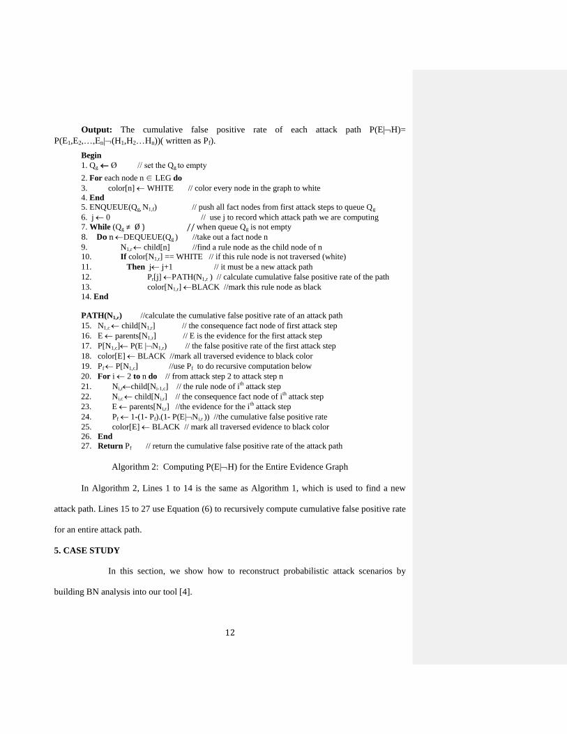
Output: The cumulative false positive rate of each attack path P(E|H)=

P(E1,E2,…,En|(H1,H2…Hn))( written as Pf).

Begin

1. Qg Ø // set the Qg to empty

2. For each node n ∈ LEG do

3. color[n] WHITE // color every node in the graph to white

4. End

5. ENQUEUE(Qg, N1,f) // push all fact nodes from first attack steps to queue Qg

6. j 0 // use j to record which attack path we are computing

7. While (Qg ≠ Ø ) // when queue Qg is not empty

8. Do n DEQUEUE(Qg ) //take out a fact node n

9. N1,r child[n] //find a rule node as the child node of n

10. If color[N1,r] == WHITE // if this rule node is not traversed (white)

11. Then j j+1 // it must be a new attack path

12. Pr[j] PATH(N1,r ) // calculate cumulative false positive rate of the path

13. color[N1,r] BLACK //mark this rule node as black

14. End

PATH(N1,r) //calculate the cumulative false positive rate of an attack path

15. N1,c child[N1,r] // the consequence fact node of first attack step

16. E parents[N1,r] // E is the evidence for the first attack step

17. P[N1,c] P(E |N1,r) // the false positive rate of the first attack step

18. color[E] BLACK //mark all traversed evidence to black color

19. Pf P[N1,c] //use Pf to do recursive computation below

20. For i 2 to n do // from attack step 2 to attack step n

21. Ni,rchild[Ni-1,c] // the rule node of ith attack step

22. Ni,c child[Ni,r] // the consequence fact node of ith attack step

23. E parents[Ni,r] //the evidence for the ith attack step

24. Pf 1-(1- Pf).(1- P(E|Ni,r )) //the cumulative false positive rate

25. color[E] BLACK // mark all traversed evidence to black color

26. End

27. Return Pf // return the cumulative false positive rate of the attack path

Algorithm 2: Computing P(E|H) for the Entire Evidence Graph

In Algorithm 2, Lines 1 to 14 is the same as Algorithm 1, which is used to find a new

attack path. Lines 15 to 27 use Equation (6) to recursively compute cumulative false positive rate

for an entire attack path.

5. CASE STUDY

In this section, we show how to reconstruct probabilistic attack scenarios by

building BN analysis into our tool [4].

13

5.1 The Experimental Network

Figure 4 shows an experimental network from [4], which we used as a case study to show

how to generate a logical evidence graph from post-attack evidence. In this network, the external

Firewall 1 controls network access from the Internet to the network, where a webserver hosts two

web services—Portal web service and Product web service. The internal Firewall 2 controls the

access to a SQL database server that can be accessed from webservers and workstations. The

administrator has administrative privilege on the Portal webserver that supports a forum for users

to chat with the administrator. We used SNORT as the IDS and configured both web servers and

the database server to log all accesses and queries as events. We examine them for attack

evidence.

Figure 4: An Experimental Attack Network

By exploiting vulnerabilities in a Windows workstation and a web server that have access

to the database server, we, who simulated the attacker, were able to successfully launch two

kinds of attacks on the database server and a Cross Site Scripting (XSS) attack towards the

administrator’s computer. These attacks include (1) using a compromised workstation to access

the database server (CVE-2009-1918), (2) exploiting the vulnerability on the web application

14

(CWE89) in the Product webserver to attack the database server, and (3) exploiting XSS

vulnerability on the chatting forum hosted by the portal web service to steal the administrator’s

session ID, which allowed the attacker to send out phishing emails to the clients, tricking them to

update their confidential information.

Our IDS and the logging system in the network detected some attack activities. We pre-

processed them to data as shown in Table 2. The post attack status obtained by using forensic

tools is also formalized to Table 3.

Table 2: Formalized Evidence of the Alerts and Log from Figure 4

Timestamp Source IP Destination IP Content/Observed Events Vulnerability

08/13-

12:26:10

129.174.124.122

Attacker

129.174.124.184

Workstation1 SHELLCODE x86 inc ebx NOOP CVE-2009-1918

08/13-

12:27:37

129.174.124.122

Attacker

129.174.124.185

Workstation2 SHELLCODE x86 inc ebx NOOP CVE-2009-1918

08/13-

14:37:27

129.174.124.122

Attacker

129.174.124.53

Product Web Server SQL Injection Attempt CWE89

08/13-

16:19:56

129.174.124.122

Attacker

129.174.124.137

Administrator Cross Site Scripting XSS

08/13-

14:37:29

129.174.124.53

Product Web Server

129.174.124.35

Database Server name='Alice' AND password='alice' or '1'='1' CWE89

…

Table 3: Post Attack Status from Attacks in Figure 4

Timestamp Attacked Computer Attack Event Post Attack Status

08/13-14:37:29 129.174.124.35

Database Server Information retrieved maliciously Malicious Access

… …

5.2 Constructing the Logical Evidence Graph

To use our Prolog-based rules for evidence graph construction, we codified evidence and

system state to instantiations of predicates that will be used in these rules, as shown in Figure 5.

In Figure 5, Line 1, 2, 3 model evidence representing post attack status (Table 3), Line 4 to 10

15

model network topology (system setup), Line 11 to 14 model system configurations, and Line 15

to 21 mode vulnerabilities obtained from captured evidence (Table 2).

//Observed Attack Events

1. attackGoal(execCode(workStation1,_)).

2. attackGoal(execCode(dbServer,user)).

3. attackGoal(execCode(clients,user)).

//Network Topology

4. attackerLocated(internet).

5. hacl(internet, webServer, tcp, 80).

6. hacl(internet, workStation1,tcp,_).

7. hacl(webServer, dbServer,tcp,3660).

8. hacl(internet,admin,_,_).

9. hacl(admin,clients,_,_).

10. hacl(workStation1,dbServer,_,_).

//Computer Configuration

11. hasAccount(employee, workStation1, user).

12. networkServiceInfo(webServer , httpd, tcp , 80 , user).

13. networkServiceInfo(dbServer , httpd, tcp , 3660 , user).

14. networkServiceInfo(workStation1 , httpd, tcp , 4040 , user).

/* Information From Table 1---software vulnearbility */

15. vulExists(webServer, 'CWE89', httpd).

16. vulProperty('CWE89', remoteExploit, privEscalation).

17. vulExists(dbServer, 'CWE89', httpd).

18. vulProperty('CWE89', remoteExploit, privEscalation).

19. vulExists(workStation1, 'CVE-2009-1918', httpd).

20. vulProperty('CVE-2009-1918', remoteExploit, privEscalation).

21. timeOrder(webServer,dbServer,14.3727,14.3729).

…

Figure 5: The Input File for Logical Evidence Graph Generation

We ran the input file on rules that represent generic attack techniques in our reasoning

system with two databases, including an anti-forensic database [4] and MITRE’s CVE [2], to

remove irrelevant evidence and find explanations for missing evidence. They are: (1) according

to MITRE CVE database, the “Workstation 2”, which is a Linux machine using Firefox as the

web browser, does not support a successful attack by using “CVE-2009-1918”, because this

exploit only succeeds on Windows Internet Explorer; (2) a new attack path representing that the

attacker launched a phishing attack toward the clients by using the administrator’s stolen session

16

ID has been found; (3) an attack path between the compromised “Workstation1” and the

database server has been found.

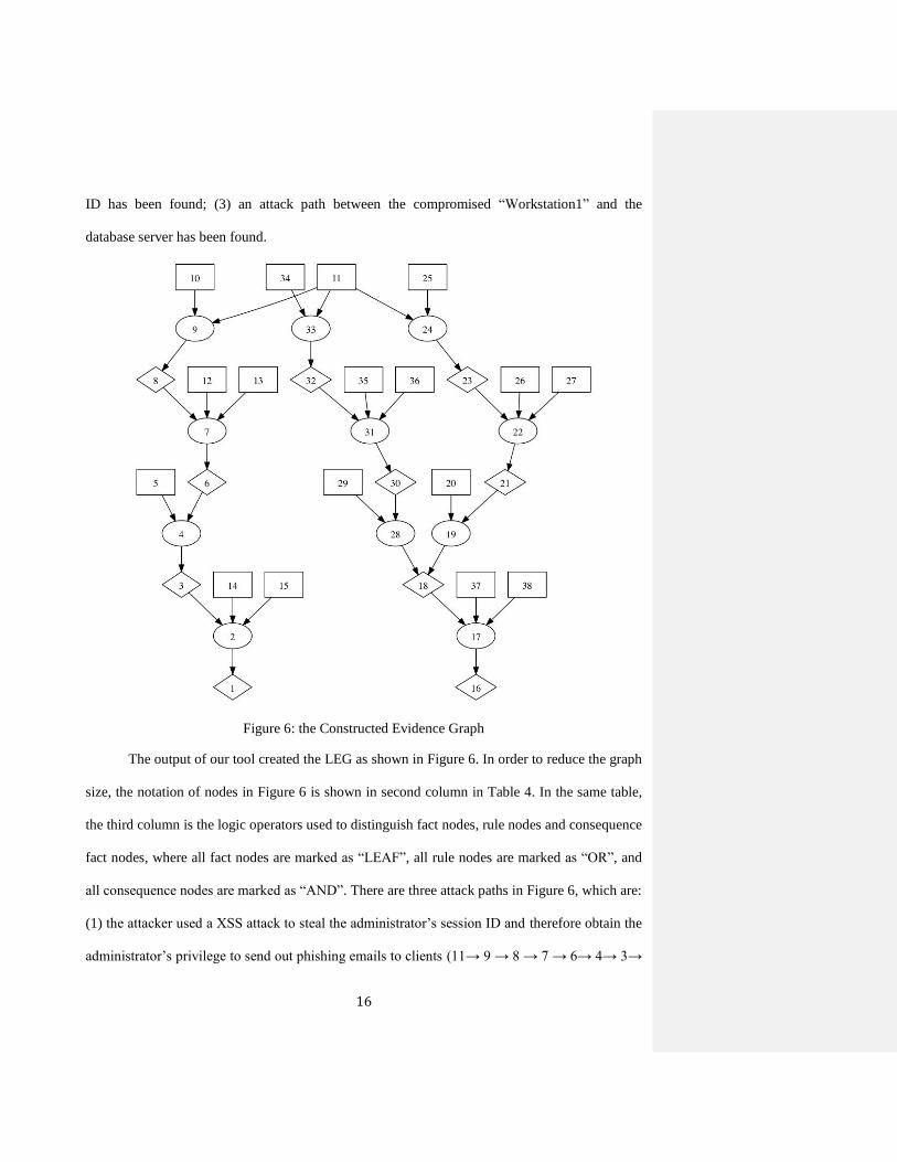
Figure 6: the Constructed Evidence Graph

The output of our tool created the LEG as shown in Figure 6. In order to reduce the graph

size, the notation of nodes in Figure 6 is shown in second column in Table 4. In the same table,

the third column is the logic operators used to distinguish fact nodes, rule nodes and consequence

fact nodes, where all fact nodes are marked as “LEAF”, all rule nodes are marked as “OR”, and

all consequence nodes are marked as “AND”. There are three attack paths in Figure 6, which are:

(1) the attacker used a XSS attack to steal the administrator’s session ID and therefore obtain the

administrator’s privilege to send out phishing emails to clients (11→ 9 → 8 → 7 → 6→ 4→ 3→

17

2→ 1)(left); (2) the attacker used a buffer overflow vulnerability (CVE-2009-1918) to

compromise a workstation, then obtained access to the database

(34→33→32→31→30→28→18→17→16) (Middle); and (3) the attacker used a web

application that does not sanitize users’ input (CWE89) to launch a SQL injection attack toward

the database (11→24→23→22→21→19→18→17→16) (right).

Table 4: the Notation of Nodes in Figure 6

Node Notation Relation

1 execCode(clients,user) OR

2 THROUGH 3 (remote exploit of a server program) AND

3 netAccess(clients,tcp,_) OR

4 THROUGH 7 (multi-hop access) AND

5 hacl(admin,clients,tcp,_) LEAF

6 execCode(admin,apache) OR

7 THROUGH 3 (remote exploit of a server program) AND

8 netAccess(admin,tcp,80) OR

9 THROUGH 8 (direct network access) AND

10 hacl(internet,admin,tcp,80) LEAF

11 attackerLocated(internet) LEAF

12 networkServiceInfo(admin,httpd,tcp,80,apache) LEAF

13 vulExists(admin,'XSS',httpd,remoteExploit,privEscalation) LEAF

14 networkServiceInfo(clients,httpd,tcp,_,user) LEAF

15 vulExists(clients,'Phishing',httpd,remoteExploit,privEscalation) LEAF

16 execCode(dbServer,user) OR

17 THROUGH 3 (remote exploit of a server program) AND

18 netAccess(dbServer,tcp,3660) OR

19 THROUGH 7 (multi-hop access) AND

20 hacl(webServer,dbServer,tcp,3660) LEAF

21 execCode(webServer,user) OR

22 THROUGH 3 (remote exploit of a server program) AND

23 netAccess(webServer,tcp,80) OR

24 THROUGH 8 (direct network access) AND

25 hacl(internet,webServer,tcp,80) LEAF

26 networkServiceInfo(webServer,httpd,tcp,80,user) LEAF

27 vulExists(webServer,'CWE89',httpd,remoteExploit,

privEscalation) LEAF

28 THROUGH 7 (multi-hop access) AND

29 hacl(workStation1,dbServer,tcp,3660) LEAF

30 execCode(workStation1,user) OR

31 THROUGH 3 (remote exploit of a server program) AND

32 netAccess(workStation1,tcp,4040) OR

33 THROUGH 8 (direct network access) AND

34 hacl(internet,workStation1,tcp,4040) LEAF

35 networkServiceInfo(workStation1,httpd,tcp,4040,user) LEAF

36 vulExists(workStation1,'CVE-2009-1918',httpd,remoteExploit,privEscalation) LEAF

18

37 networkServiceInfo(dbServer,httpd,tcp,3660,user) LEAF

38 vulExists(dbServer,'CWE89',httpd,remoteExploit,privEscalation) LEAF

5.3 Calculate Posterior Probabilities and False Positives

In this Section, we use Algorithm 1 and Algorithm 2 to calculate P(H|E1,E2..En) and

P(E1,E2..En |H) for attack paths in Figure 6 (H is H1∩ H2…∩Hn ).

5.3.1 Using Algorithm 1 to Calculate P(H|E1,E2..En)

Algorithm 1 requires [P(N1,r), P(N1,f ), P(N1,f | N1,r) ], [P(Ni,r), P(Ni-1,c, Ni,f | Ni,r), P(Ni-1,c ,

Ni,f) (i=1 to n)]. All these probabilities are obtained from expert knowledge. To minimize the

subjectivity of the impact, we suggest using the average probability computed from many

forensic experts’ judgments [7]. Because the case study mainly focuses on the computation, for

simplicity, we let all P(Hi) = P(Hi) = 50%, P(Ei) =k ∈ [0,1]( “k” differs for different evidence

in real scenarios), and assigned P(Ei|Hi) by using our own judgment (the probability of P(Ei|Hi) is

listed in Table 5). Thus, the P(Hi|Ei) for every attack step without considering about other attack

steps is 𝑃(Hi)𝑃(Ei|Hi)

𝑃(Ei)=

0.5.𝑃(Ei|Hi)

𝑘=

𝑃(Ei|Hi)

2𝑘=c.P(Ei|Hi) ( let c=1/(2k)). By using Algorithm 1, we

obtained P(H|E1,E2..En) as shown in the last column of Table 5.

Table 5: Use Algorithm 1 to Compute P(H|E1…En) for Attack Paths in Figure 6

Attack Path Attack Step 1 Attack Step 2

H1 P(E1|H1) P(H1|E1) P(H|E1) H2 P(E2|H2) P(H2|E2) P(H|E1,E2)

Left Node 9 0.9 0.9c 0.9c Node 7 0.8 0.8c 0.72c^2

Middle Node 33 0.99 0.99c 0.99c Node 31 0.87 0.87c 0.861c^2

Right Node 24 0.99 0.99c 0.99c Node 22 0.85 0.85c 0.842c^2

Attack Path Attack Step 3 Attack Step 4

H3 P(E3|H3) P(H3|E3) P(H|E1,E2,E3) H4 P(E4|H4) P(H4|E4) P(H|E1,E2,E3,E4)

Left Node 4 0.9 0.9c 0.648c^3 Node 2 0.75 0.75c 0.486c^4

Middle Node 28 0.87 0.87c 0.75c^3 Node 17 0.75 0.75c 0.563c^4

Right Node 19 0.97 0.97c 0.817c^3 Node 17 0.95 0.95c 0.776c^4

19

Notice Node 17 has two joint posterior probabilities, which are from middle path and

right path respectively. We can notice that the attack path from the former has a smaller

probability than the latter. That is because the attacker destroyed the evidence obtained from the

middle path that involves using a compromised workstation to get access to the databases.

Correspondingly, the P(Ei|Hi) is smaller. Therefore, the corresponding hypothesized attack path

has a much smaller probability P(H|E1,E2..En). In reality, it is unlikely that the same attacker

would try a different attack path to attack the same target if he already succeeded. A possible

scenario would be that the first attack path was not expected, so the attacker tried the second

attack path to launch the attack. The joint posterior probability P(H|E1,E2...En) could help

investigator to select the most pertinent attack path.

5.3.2 Using Algorithm 2 to Calculate P(E1,E2..En |H )

Algorithm 2 requires P(N1,f|N1,r) as P(E1|H1), P(Ni-1,c,Ni,f |Ni,r) as P(Ei|Hi)(i=2 to n) to

recursively compute P(E1,E2..En |H). As an example, we assigned P(Ei| Hi) for different attack

step in the three attack paths in Table 6 and calculated P(E1,E2..En |H). The results show that

the right attack path has the smallest cumulative false positive estimate.

Table 6: Use Algorithm 2 to Calculate P(E1,E2..En |H )

Attack Path Attack Step 1 Attack Step2

H1 P(E1|¬H1) P(E1|¬H1) H2 P(E2|¬H2) P(E1,E2|¬H)

Left Node 9 0.002 0.002 Node 7 0.001 0.003

Middle Node 33 0.002 0.002 Node 31 0.003 0.005

Right Node 24 0.002 0.002 Node 22 0.001 0.003

Attack path Attack Step3 Attack Step4

H3 P(E3|¬H3) P(E1,E2,E3|¬H) H P(E4|¬H4) P(E1,E2,E3,E4|¬H)

Left Node 4 0.004 0.007 Node 2 0.03 0.0368

Middle Node 28 0.003 0.008 Node 17 0.04 0.0477

Right Node 19 0.002 0.005 Node 17 0.007 0.012

20

Values computed for P(H|E1,E2..En) and P(E1,E2..En |H) show our belief on the three

constructed attack paths given the collected evidence. The right attack path

(11→24→23→22→21→19→18→17→16) is the most convincing one, because it has the

largest P(H|E) and smallest P(E|¬H). The left path is not convincing, because its joint posterior

probability is less than 0.5c^4. The middle path is not so convincing because it has a bigger

cumulative false positive rate, suggesting that the attack path should be re-evaluated to determine

if reflects a real attack scenario.

6. CONCLUSION

In this paper, we have described a method that uses rules to construct a LEG and maps it

to a BN so that the joint posterior probability or false positive rate for the constructed attack

paths could be computed automatically. By using a case study, we showed how our method

could guide forensic investigators to choose the most likely attack scenarios that fit the available

evidence. Our case study showed our method and the accompany tool could help network

forensic experts save time and effort in forensic investigation and analysis. However, our system

does not provide a way to resolve zero-day attack problems. Our ongoing work extends our

current model to address zero-day vulnerabilities.

DISCLAIMER

This paper is not subject to copyright in the United States. Commercial products are identified in

order to adequately specify certain procedures. In no case does such identification imply

recommendation or endorsement by the National Institute of Standards and Technology, nor

does it imply that the identified products are necessarily the best available for the purpose.

REFERENCES:

21

[1] B. A. Olshausen, "Bayesian probability theory." The Redwood Center for Theoretical

Neuroscience, Helen Wills Neuroscience Institute at the University of California at Berkeley,

Berkeley, CA (2004).

[2] MITRE Common Vulnerabilities and Exposures. Retrieved from https://cve.mitre.org/.

[3] J. Pearl, "Fusion, propagation, and structuring in belief networks". Artificial intelligence 29.3

(1986): 241-288.

[4] C. Liu, A. Singhal, D. Wijesekara, “A Logic Based Network Forensics Model for Evidence

Analysis”. IFIP International Conference on Digital Forensics, Orlando, Florida, January 24-26

2015.

[5] A. Darwiche, “Modeling and Reasoning with Bayesian Networks”. Cambridge University

Press, April 06, 2009.

[6] F. Taroni, A. Biedermann, P. Garbolino, C.G. Aitken, “A general approach to Bayesian

networks for the interpretation of evidence”. Forensic Sci. Int., 139 (2004), pp. 5–16.

[7] M Kwan, K P Chow, F Law and P Lai, “Reasoning About Evidence using Bayesian

Network”. Advances in Digital Forensics IV, International Federation for Information Processing

(IFIP) January 2008, Tokyo, pp.141-155.

[8] B. Carrier, “A Hypothesis-Based Approach to Digital Forensic Investigations (Ph.D.

Thesis)”, 2006,West Lafayette: Purdue University.

[9] Y. Liu, H. Man, “Network vulnerability assessment using Bayesian Networks”. In

Proceedings of SPIE - Data Mining, Intrusion Detection, Information Assurance and Data

Networks Security (SPIE’05), pages 61–71, 2005.

[10] C. Vlek, H. Prakken, S. Renooij and B. Verheij(2013), “Modeling crime scenarios in a

Bayesian Network”. The 14th International Conference on Artificial Intelligence and Law

(ICAIL 2013), Proceedings of the Conference, 150–159, ACM Press, New York.

[11] Fenton, N., Neil, M., & Lagnado, D.A. (2012), “A general structure for legal arguments

about evidence using Bayesian networks”. Cognitive Science, 37, 61–102.

[12] F. Taroni, S. Bozza, A. Biedermann, G. Garbolino, C.G.G. Aitken, “Data Analysis in

Forensic Science: A Bayesian Decision Perspective”. John Wiley & Sons, Chichester (2010).

[13] X Ou, W. F. Boyer, M. A. McQueen, “A scalable approach to attack graph generation”. In:

13th ACM Conference on Computer and Communications Security (CCS), pp. 336–345 (2006).

[14] MulVAL: A logic-based enterprise network security analyzer. Retrieved from

http://www.arguslab.org/mulval.html.