Contests Between Players With Mean-Variance Preferences

Alex Robson

No. 2012-07

Series Editor: Associate Professor Fabrizio Carmignani

Copyright © 2012 by the author(s). No part of this paper may be reproduced in any form, or stored in a retrieval system, without prior permission of the author(s).

1

Contests Between Players With Mean-Variance Preferences

Alex Robson*

Abstract

We study contests between players who care only about the mean and variance of lotteries. This framework admits situations where players may not obey the axioms of expected utility maximization. If there are only two identical players in the contest, then we obtain a general irrelevance result: even though the players are variance-averse, in equilibrium they will act as if they are not. If there are more than two identical players, then attitudes towards variance influence the equilibrium efforts and the outcome: variance-averse players dissipate less rent than variance-neutral players. However, this effect disappears as the number of players increases, and when the number of players becomes very large, we obtain an approximate irrelevance result: players “almost” act as if their variance-aversion does not matter. Finally, we show that in asymmetric contests where players have different coefficients of variance aversion, the less variance-averse player will not necessarily exert more effort than the more variance-averse player.

Keywords: Contests, Risk Aversion, Expected Utility.

JEL Codes: C72, D72, D81.

* Department of Accounting, Finance and Economics, Griffith Business School, Nathan Campus, Nathan, Qld, 4111. email: a.robson@griffith.edu.au

2

1. Introduction The issue of how players’ risk aversion affects effort and rent dissipation arises frequently in the theoretical analysis of contests, and also in applications of this theory to rent-seeking behaviour, litigation, violent conflict and political campaigning.1 Risk averse players have a desire to avoid large losses and may exert greater effort in order to achieve this objective. For example, Skaperdas (1991) shows that when the size of the prize is endogenous, then the more risk averse both contest participants become, the greater the amount of resources that are devoted to conflict.

However, this result is far from general. Hillman and Katz (1984) analyse rent-seeking contests with a large number of players (the so-called “competitive” case) and find that rent dissipation declines as risk aversion increases. On the other hand, Konrad and Schlesinger (1997) examine a model with symmetric players but with general utility functions in an expected utility framework, and show that an increase risk aversion has an ambiguous effect on rent dissipation. In other words, they show that it is possible for the contest with identical risk-averse players to dissipate more of the rents than the same contest with risk-neutral players. Treich (2009) extends this result by showing that if risk-averse players are also prudent (in the sense that the third derivative of the utility function is non-negative), then risk aversion always decreases efforts compared to the case of risk-neutral players. Finally, Cornes and Hartley (2012) study contests between players who exhibit loss aversion, and find that if the degree of loss aversion is sufficiently large, there may be multiple equilibria. They also show that in the presence of other asymmetric equilibria, the symmetric equilibrium may display perverse comparative statics (for example, it is possible for aggregate expenditure to be decreasing in the number of players).

Another question of interest is whether a less risk averse player exerts more effort than his more risk averse opponent(s). Skaperdas and Gan (1995) study rent seeking games with an exogenous prize when players have constant absolute risk aversion (CARA) preferences, and show that a less risk averse player will exert more effort than his more risk-averse opponent, and will therefore have a higher probability of winning.

Cornes and Hartley (2009) study asymmetric contests with risk averse players, and extend these earlier results by showing that for asymmetric contests with prudent risk-averse contestants who not too large (as measured by their equilibrium probability of winning, aggregate lobbying effort is smaller than in a second contest with the same contest success function but risk-neutral contestants.

1 See Konrad (2009) for a thorough survey of contest theory and its applications. Robson and Skaperdas (2008) analyse litigation and settlement using contests, and Chapter 11 of Robson (2012) explores implications of contest theory for the market for lawyers.

3

To gain a deeper understanding of the effect of attitudes toward risk on effort in contests, this paper studies contests in the familiar mean-variance framework of introductory finance theory.2 The power of the mean-variance model is that offers a simple and intuitive structure in which to analyse the effects of risk on individual incentives and aggregate market outcomes in a wide variety of interesting situations. For example, as is well known, the framework is one of the key assumptions in the standard Capital Asset Pricing Model (CAPM), which is ubiquitous in the finance literature.3

However, the mean variance framework also has its conceptual and theoretical disadvantages. Foremost among these is that if the model is to be consistent with the axioms of expected utility (EU) maximisation, it can only be applied in a limited set of circumstances. One instance that leads to preferences over only the first two moments of the lottery within the EU framework is when individuals are assumed to have quadratic preferences. Another modelling strategy is to restrict the underlying distributions of the set of lotteries being chosen (i.e. assets or portfolios in the finance setting) to those that can be completely characterised by their first and second moments (for example, the Normal distribution).

In other instances, the mean-variance model may not be consistent with expected utility maximisation. However, all of the CAPM results still obtain. Hence, if one is willing to work outside the assumptions of expected utility maximisation, then the mean-variance framework is quite useful In addition, it has some attractive theoretical properties. For example, Loffler (1996) shows that a preference relation is strictly variance averse and strictly monotonic in the riskless asset if and only if the representing utility function fulfills the μ-σ2 criterion. Epstein (1985) adopts a range of general postulates regarding declining absolute risk aversion, and shows that these imply mean-variance preferences.

Our analysis focuses on the extent to which variance-aversion affects incentives and behaviour in symmetric contests. The paper is structured as follows. Section 2 presents two examples to illustrate the main issues. Section 3 explores a more general setup with mean variance preferences. Section 4 explores the case with two asymmetric players. Section 5 concludes.

2. Two Illustrative Examples Before considering the general case, this section presents two examples of contests in which the players have mean-variance preferences that are frequently encountered in microeconomic analysis and the theory of finance.

2 Markowitz (1959), Tobin (1958) are the original papers. Chipman (1973) and Chamberlain (1983) conducted further analyses of mean-variance preferences and their implications.

3 See, for example, Hirshleifer and Riley (1992), page 156.

4

2.1 Expected Utility Maximisation with Quadratic Utility Functions

For an example of mean-variance preferences which are consistent with expected utility maximization, suppose that each player ranks amounts of wealth received with certainty according to the quadratic utility function:

( ) ( )212i i i iu w w b w= − (1)

where 0b > . Let iw w= for all i .4 As is well known, this means that each player ranks lotteries according to the following mean-variance criterion:

( )

( ) ( ) ( )

2 2

2 2

12

1 1, , 12 2

i i i i i

i i i i i i i i i i

u w b

w p x x R x b w p x x R x b R p p

µ µ σ

− −

= − +

= + − − + − − −

E

We assume that w R> , and to ensure that utility is increasing, we assume that 1 w Rb> + . Together, these assumptions are sufficient to guarantee the uniqueness of

equilibrium. 5

The first order conditions yield:

( ) ( )211 1 1 2 02

i ii i

i i

p pR b bR px x

µ ∂ ∂

− − − − = ∂ ∂

The assumption that 1 w Rb> + implies that 1 0ibµ− > . We assume the following

contest success function (CSF):6

4 In a contest framework, these preferences have been considered by Cornes and Hartley (2009) and Treich (2008)

5 Cornes and Hartley (2009) show that a sufficient condition for uniqueness is that 2 '( ) '( )u R x u x− ≥ − for all (0, )x R∈ . With the quadratic preferences in (1), we have

'( ) 1u w bw= − and so a sufficient condition is 2[1 ( )] 1b R x bx− − ≥ + for all (0, )x R∈ , or

1 2R xb≥ − for all (0, )x R∈ . The assumptions that w R> and

1 w Rb> + ensure that this

condition is satisfied. 6 See Skaperdas (1996) for an axiomatization of this CSF.

5

( )if 0

,1 otherwise

ij ii j

j ii ji i i

x x xx x

p x

n

≠≠

−

+ >∑ +∑=

x (2)

For the purposes of our analysis, the key feature of the CSF in (2) is the anonymity property: each player’s probability success does not depend on their identity or the identities of their opponents, but just on each player’s effort.7 Then, in a symmetric

equilibrium, we have 2

1 1 and ii

i

p npn x n x

∂ −= =

∂, and so:

( ) 22 2

1 1 1 21 1 ( ) 12

n nR b w R x bRn x n n− − − − + − = −

(3)

If there are only 2 players, then the right hand side of (3) is zero. Since 1 w Rb> + ,

we have 1 ( ) 0b w R x− + − > , and so this implies that 2

1 1 0n Rn x−

− = , or 4Rx = , which

is identical to the case where b=0.

On the other hand, if there are more than two players, then the right hand side of (3) is

positive, and since 1 ( ) 0b xµ− < , this implies that 2

1 1 0n Rn x−

− > , or 2

1nx Rn−

< .

We therefore obtain:

Proposition 1: (a) In a contest between two identical agents with quadratic preferences, the players behave as if they have linear preferences, and any aversion to risk is irrelevant.

(b) If there are more than two players with quadratic preferences, the individual and aggregate equilibrium rent seeking effort is less than if the players were risk neutral.

2.2 Non-Expected Utility Maximizers

We now assume that each player has preferences of the familiar form:

( ) ( )

2

2

12

1, 12

i i

i i i i i i

V b

w p x x R x b R p p

µ σ

−

= −

= + − − −

(4)

7 This is axiom A3 of Skaperdas (1996)

6

It is well known in the finance literature that if an agent is choosing from a family of normally distributed random variables, then the preferences in (3) can be derived by assuming that individuals are expected utility maximizers with constant absolute risk aversion (CARA) parameter b .

However, in a rent-seeking situation, the underlying family of random variables is not normally distributed. As far as the individual rent-seeker is concerned, there are only two outcomes or states of the world that are relevant for each player. If each player takes the other players' efforts as given, we can regard their own choice of effort as the act of choosing a single element from the family of two-point distributions or Bernoulli random variables, where the underlying outcome space for each member of this family is simply { }Win, Lose .

As we show in the Appendix to this paper, when the players in the contest have the preferences in (4), they violate the independence axiom. In other words, these preferences must represent the behaviour of players who do not maximise expected utility.

The first order conditions are now:

( )211 1 2 02

i ii

i i

p pR bR px x∂ ∂

− − − =∂ ∂

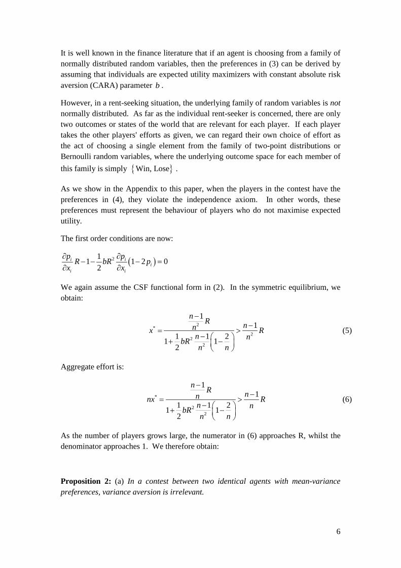
We again assume the CSF functional form in (2). In the symmetric equilibrium, we obtain:

2

*2

22

11

1 1 21 12

n R nnx Rn nbRn n

−−

= >− + −

(5)

Aggregate effort is:

*

22

11

1 1 21 12

n R nnnx Rn nbRn n

−−

= >− + −

(6)

As the number of players grows large, the numerator in (6) approaches R, whilst the denominator approaches 1. We therefore obtain:

Proposition 2: (a) In a contest between two identical agents with mean-variance preferences, variance aversion is irrelevant.

7

(b) If there are more than two players having mean-variance preferences, the equilibrium individual and aggregate efforts are less than if the players were not variance averse.

(c) In the limit, as the number of players grows large, aggregate effort in the variance-averse case approaches the same limit as aggregate effort in the variance-neutral case.

In other words, variance aversion of the kind embodied in (4) makes absolutely no difference to individual and aggregate outcomes when there are two identical players, and “almost” no difference when there are a large number of identical players. For all other cases, variance aversion reduces individual and aggregate effort.

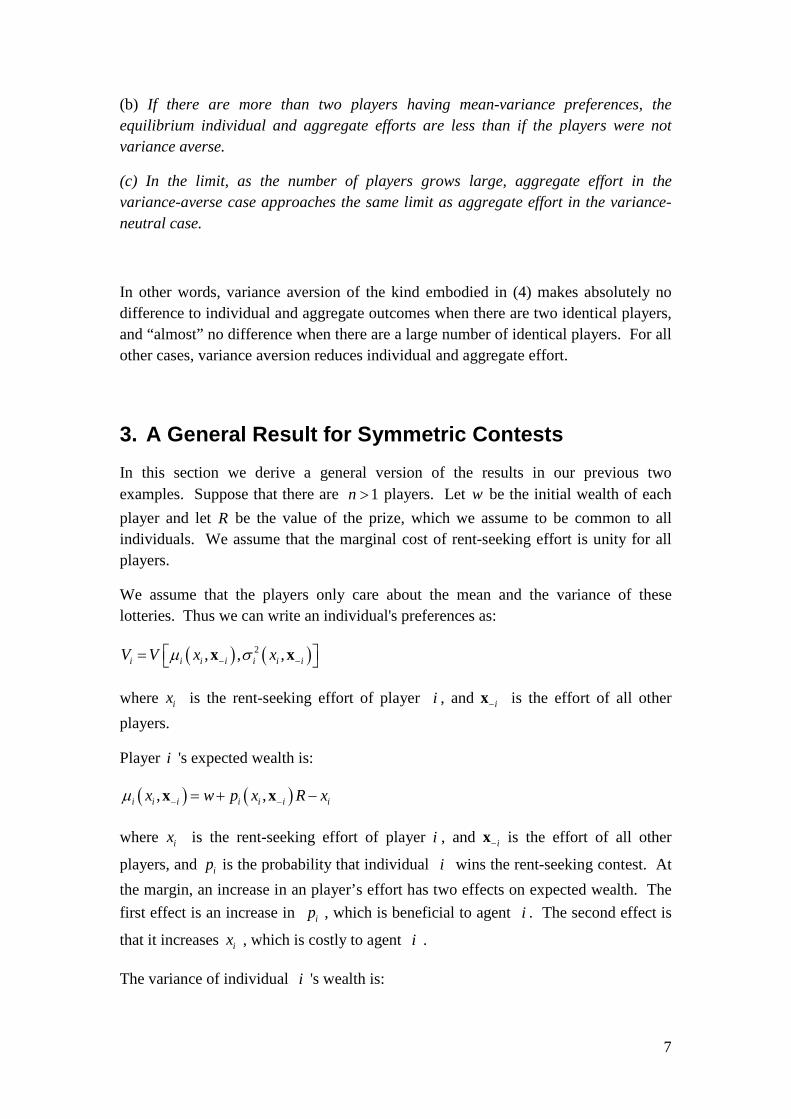
3. A General Result for Symmetric Contests In this section we derive a general version of the results in our previous two examples. Suppose that there are 1n > players. Let w be the initial wealth of each player and let R be the value of the prize, which we assume to be common to all individuals. We assume that the marginal cost of rent-seeking effort is unity for all players.

We assume that the players only care about the mean and the variance of these lotteries. Thus we can write an individual's preferences as:

( ) ( )2, , ,i i i i i i iV V x xµ σ− − = x x

where ix is the rent-seeking effort of player i , and i−x is the effort of all other players.

Player i 's expected wealth is:

( ) ( ), ,i i i i i i ix w p x R xµ − −= + −x x

where ix is the rent-seeking effort of player i , and i−x is the effort of all other

players, and ip is the probability that individual i wins the rent-seeking contest. At the margin, an increase in an player’s effort has two effects on expected wealth. The first effect is an increase in ip , which is beneficial to agent i . The second effect is

that it increases ix , which is costly to agent i .

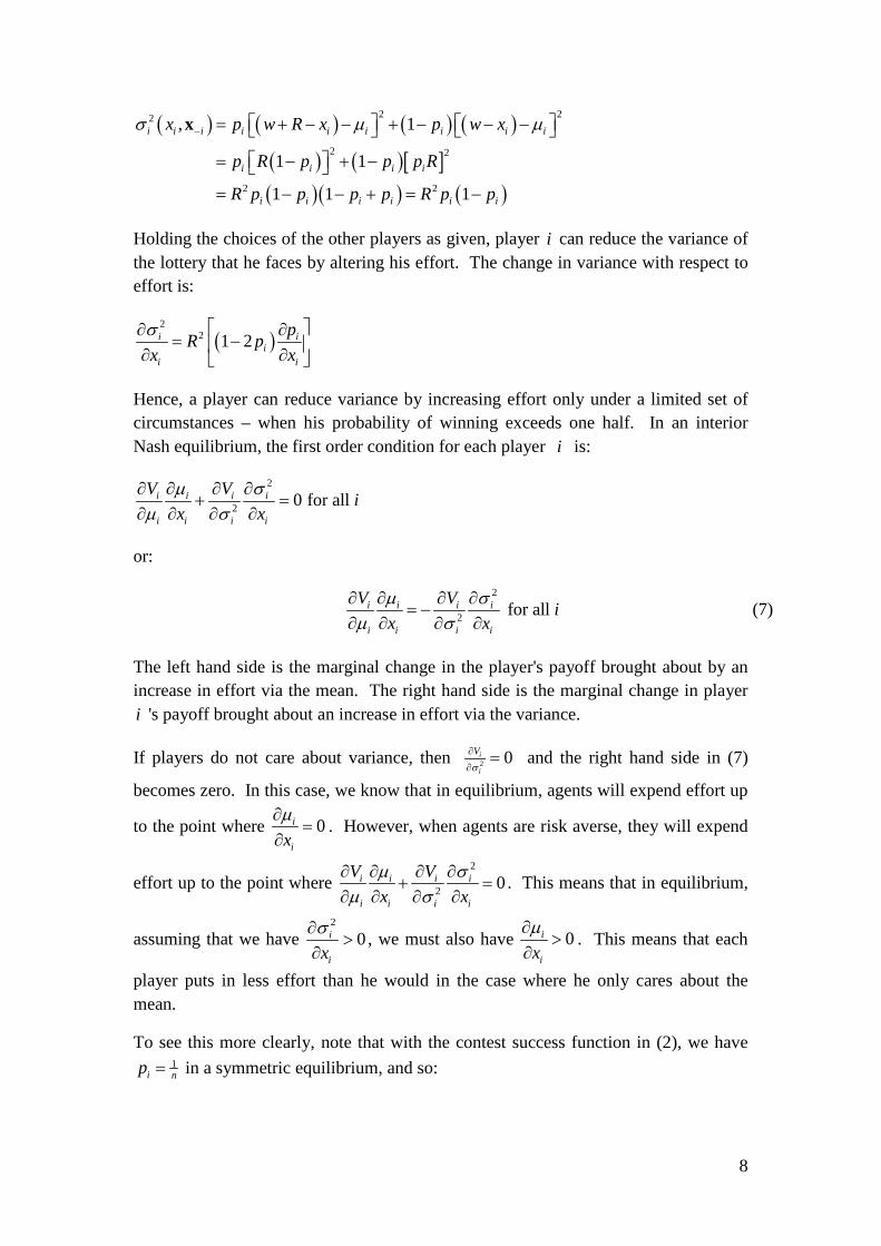
The variance of individual i 's wealth is:

8

( ) ( ) ( ) ( )

( ) ( )[ ]( )( ) ( )

2 22

2 2

2 2

, 1

1 1

1 1 1

i i i i i i i i i

i i i i

i i i i i i

x p w R x p w x

p R p p p R

R p p p p R p p

σ µ µ− = + − − + − − −

= − + − = − − + = −

x

Holding the choices of the other players as given, player i can reduce the variance of the lottery that he faces by altering his effort. The change in variance with respect to effort is:

( )2

2 1 2i ii

i i

pR px xσ ∂ ∂

= − ∂ ∂

Hence, a player can reduce variance by increasing effort only under a limited set of circumstances – when his probability of winning exceeds one half. In an interior Nash equilibrium, the first order condition for each player i is:

2

2 0 for all i i i i

i i i i

V V ix xµ σ

µ σ∂ ∂ ∂ ∂

+ =∂ ∂ ∂ ∂

or:

2

2 for all i i i i

i i i i

V V ix xµ σ

µ σ∂ ∂ ∂ ∂

= −∂ ∂ ∂ ∂

(7)

The left hand side is the marginal change in the player's payoff brought about by an increase in effort via the mean. The right hand side is the marginal change in player i 's payoff brought about an increase in effort via the variance.

If players do not care about variance, then 2 0i

i

Vσ∂

∂= and the right hand side in (7)

becomes zero. In this case, we know that in equilibrium, agents will expend effort up

to the point where 0i

ixµ∂

=∂

. However, when agents are risk averse, they will expend

effort up to the point where 2

2 0i i i i

i i i i

V Vx xµ σ

µ σ∂ ∂ ∂ ∂

+ =∂ ∂ ∂ ∂

. This means that in equilibrium,

assuming that we have 2

0i

ixσ∂

>∂

, we must also have 0i

ixµ∂

>∂

. This means that each

player puts in less effort than he would in the case where he only cares about the mean.

To see this more clearly, note that with the contest success function in (2), we have 1

i np = in a symmetric equilibrium, and so:

9

22

21 1 0i i i i

i i i i

V p V pR Rx x nµ σ

∂ ∂ ∂ ∂ − + − = ∂ ∂ ∂ ∂

This implies that:

22

21 1i i i i

i i i i

V p V pR Rx x nµ σ

∂ ∂ ∂ ∂ − = − − ∂ ∂ ∂ ∂

and since 2 0i

i

Vσ∂∂

< , we therefore have:

1 0i i

i i

V p Rxµ

∂ ∂− > ∂ ∂

This implies that:

1i

i

p Rx∂

>∂

(8)

In equilibrium, the marginal benefit of an individual's rent-seeking effort must be greater than unity. However, with risk neutral expected utility maximisers, marginal benefit is exactly equal to unity, and so the inequality in (8) means that if there are

2n > identical players, they must each put in less effort in equilibrium than if they were risk neutral. In other words, as long as players are identical, aversion to variance reduces individual rent seeking effort in equilibrium.

4. Asymmetric Contests Thus far we have only considered contests in which players are identical. As discussed in the introduction, a common question in the contest literature is whether a more risk-averse player will exert more or less effort than a less risk averse player. In this section we therefore consider a similar question, but where the contest is between two variance-averse players with different preferences. Livshits (2003) argues that a natural measure or coefficient of “variance aversion” is the marginal rate of substitution along an indifference curve in mean-variance space, i.e.:

2

2

V

r Vσ

µ

∂∂= −∂∂

(9)

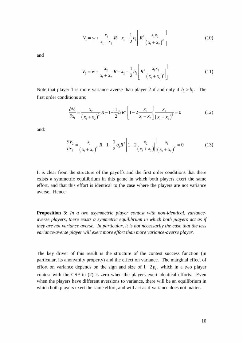
Hence, the preferences in (4) have a constant coefficient of variance aversion (CCVA). The payoffs are now:

10

( )

21 1 21 1 1 2

1 2 1 2

12

x x xV w R x b Rx x x x

= + − −

+ + (10)

and

( )

22 1 22 2 2 2

1 2 1 2

12

x x xV w R x b Rx x x x

= + − −

+ + (11)

Note that player 1 is more variance averse than player 2 if and only if 1 2b b> . The first order conditions are:

( ) ( )

21 2 1 212 2

1 1 21 2 1 2

11 1 2 02

V x x xR b Rx x xx x x x

∂= − − − = ∂ ++ +

(12)

and:

( ) ( ) ( )

22 1 2 122 2

2 1 21 2 1 2

11 1 2 02

V x x xR b Rx x xx x x x

∂= − − − =

∂ ++ + (13)

It is clear from the structure of the payoffs and the first order conditions that there exists a symmetric equilibrium in this game in which both players exert the same effort, and that this effort is identical to the case where the players are not variance averse. Hence:

Proposition 3: In a two asymmetric player contest with non-identical, variance-averse players, there exists a symmetric equilibrium in which both players act as if they are not variance averse. In particular, it is not necessarily the case that the less variance-averse player will exert more effort than more variance-averse player.

The key driver of this result is the structure of the contest success function (in particular, its anonymity property) and the effect on variance. The marginal effect of effort on variance depends on the sign and size of 1 2 ip− , which in a two player contest with the CSF in (2) is zero when the players exert identical efforts. Even when the players have different aversions to variance, there will be an equilibrium in which both players exert the same effort, and will act as if variance does not matter.

11

5. Conclusion In a contest situation, an increase in one’s effort increases the probability of obtaining the prize, which increases the mean of the outcome. On the other hand, as we have shown in this paper, increasing the probability that the favourable outcome (winning) will occur also tends to lead to an increase in the variance of the outcome, but only if a player’s probability of winning is less than a half. In contests with two players, assumptions of symmetry in the contest success function mean that there will exist a symmetric equilibrium in which the players’ influence on variance is non-existent, and they behave as if variance-aversion is irrelevant. In other cases, if players are variance averse, higher effort comes with an additional cost, and there will be a tradeoff between mean and variance. In symmetric contests, variance averse players will tend to put in less effort compared to variance-neutral players.

12

Appendix This appendix shows that for binary random variables, mean-variance preferences of the form:

212

V bµ σ= −

violate the independence axiom of expected utility theory. Let ,X Y and Z be three binary random variables, and let 0 1β< < . Now consider the following compound lotteries:

( )1F X Zβ β= ⊕ −

and

( )1G Y Zβ β= ⊕ −

The independence axiom states that for all such X , Y and Z and for all ( )0,1β ∈ , X Y if and only if F G . 8 Thus, to show that mean-variance

preferences violate the independence axiom, we need only exhibit one counterexample where this equivalence does not hold. Consider the following counterexample. Suppose that X has the following distribution:

0 with probability 11 with probability

pX

p−

=

where 120 p< < and suppose Y has the following distribution

0 with probability 11 with probability

pY

pε

ε− −

= +

where 0 pε< < . Then:

X Yp pµ ε µ= < + =

and:

( ) ( )( )2 21 1X Yp p p pσ ε ε σ= − < − − + =

Now

8See, for example, Mas-Colell, Whinston and Green, page 172.

13

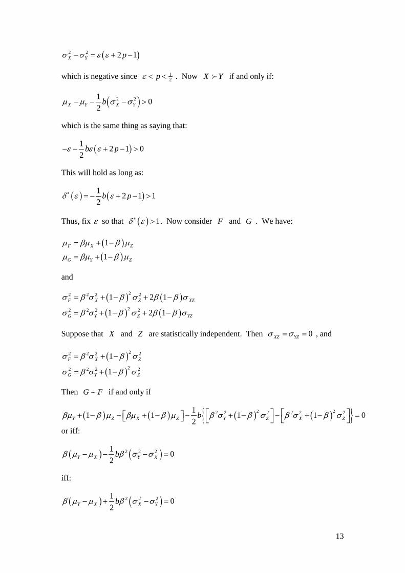
( )2 2 2 1X Y pσ σ ε ε− = + −

which is negative since 12pε < < . Now X Y if and only if:

( )2 21 02X Y X Ybµ µ σ σ− − − >

which is the same thing as saying that:

( )1 2 1 02

b pε ε ε− − + − >

This will hold as long as:

( ) ( )1 2 1 12

b pδ ε ε∗ = − + − >

Thus, fix ε so that ( ) 1δ ε∗ > . Now consider F and G . We have:

( )( )1

1F X Z

G Y Z

µ βµ β µ

µ βµ β µ

= + −

= + −

and

( ) ( )( ) ( )

22 2 2 2

22 2 2 2

1 2 1

1 2 1

F X Z XZ

G Y Z YZ

σ β σ β σ β β σ

σ β σ β σ β β σ

= + − + −

= + − + −

Suppose that X and Z are statistically independent. Then 0XZ YZσ σ= = , and

( )( )

22 2 2 2

22 2 2 2

1

1

F X Z

G Y Z

σ β σ β σ

σ β σ β σ

= + −

= + −

Then G F∼ if and only if

( ) ( ) ( ) ( ){ }2 22 2 2 2 2 211 1 1 1 02Y Z X Z Y Z X Zbβµ β µ βµ β µ β σ β σ β σ β σ + − − + − − + − − + − =

or iff:

( ) ( )2 2 21 02Y X Y Xbβ µ µ β σ σ− − − =

iff:

( ) ( )2 2 21 02Y X X Ybβ µ µ β σ σ− + − =

14

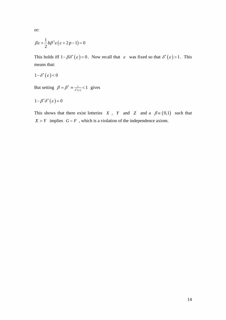
or:

( )21 2 1 02

b pβε β ε ε+ + − =

This holds iff ( )1 0βδ ε∗− = . Now recall that ε was fixed so that ( ) 1δ ε∗ > . This

means that:

( )1 0δ ε∗− <

But setting ( )1 1

δ εβ β ∗

∗= ≡ < gives

( )1 0β δ ε∗ ∗− =

This shows that there exist lotteries X , Y and Z and a ( )0,1β ∈ such that

X Y implies G F∼ , which is a violation of the independence axiom.

15

References Chamberlain, G. (1983) “A Characterisation of the Distributions that Imply Mean-Variance Utility Functions,” 29: 185-201.

Chipman, J. (1973) “The Ordering of Portfolios in Terms of Mean and Variance,” Review of Economic Studies, 40(2): 167-190.

Cornes, R. and Hartley, R. (2003) “Risk Aversion, Heterogeneity and Contests,” Public Choice, 117: 1-25.

Cornes, R. and Hartley, R. (2009) “Risk Aversion in Symmetric and Asymmetric Contests,” Economic Theory, forthcoming.

Cornes, R. and Hartley, R. (2012) “Loss Aversion in Contests,” Economics Discussion Paper Series EDP-1204, University of Manchester, January.

Epstein, L. (1985) “Decreasing Risk Aversion and Mean-Variance Analysis,” Econometrica, 53(4): 945-961.

Hillman, A. and Katz, E. (1984) "Risk Averse Rent Seekers and the Social Costs of Monopoly Power," Economic Journal, 94: 104-110.

Hirshleifer, J. and Riley, J. (1992) The Analytics of Uncertainty and Information, Cambridge: Cambridge University Press.

Konrad, K. (2009) Strategy and Dynamics in Contests, New York: Oxford University Press.

Konrad, K. and Schlesinger, H. (1997) "Risk Aversion in Rent-Seeking and Rent-Augmenting Games", Economic Journal, 107: 1671-1683.

Livshits, I. (2003) “Variance Aversion in the Small and Large,” mimeo, University of Western Ontario.

Loffler, A. (1996) “Variance Aversion Implies μ-σ2 Preferences,” Journal of Economic Theory, 69: 532-569.

Markowitz, H. (1959) Portfolio Selection: Efficient Diversification of Investments, New York: Wiley.

Mas-Colell, A., Whinston, M. and Green, J. (1991) Microeconomic Theory, London: Oxford University Press.

Robson, A. and Skaperdas, S. (2008) “Costly Enforcement of Property Rights and the Coase Theorem,” Economic Theory, 36: 109-128.

Robson, A. (2012) Law and Markets, London: Palgrave Macmillan.

Skaperdas, S. (1991) "Conflict and Attitudes Towards Risk," American Economic Review, 81(2): 116-120.

Skaperdas, S. (1996) “Contest Success Functions,” Economic Theory, 7: 283-290.

16

Skaperdas, S. and Gan, L. (1995) “Risk Aversion in Contests,” Economic Journal, 105(431): 951-962.

Tobin, J. (1958) “Liquidity Preference as Behaviour Towards Risk,” Review of Economic Studies, 25: 65-85.

Treich, N. (2009) “Risk-Aversion and Prudence in Rent-seeking Games,” Public Choice, 145(3): 339-349.