MATLAB Workbook

ENGR 154 Introduction to Engineering Mathematics

First Edition

Authors: Perrine PepiotVadim Khayms

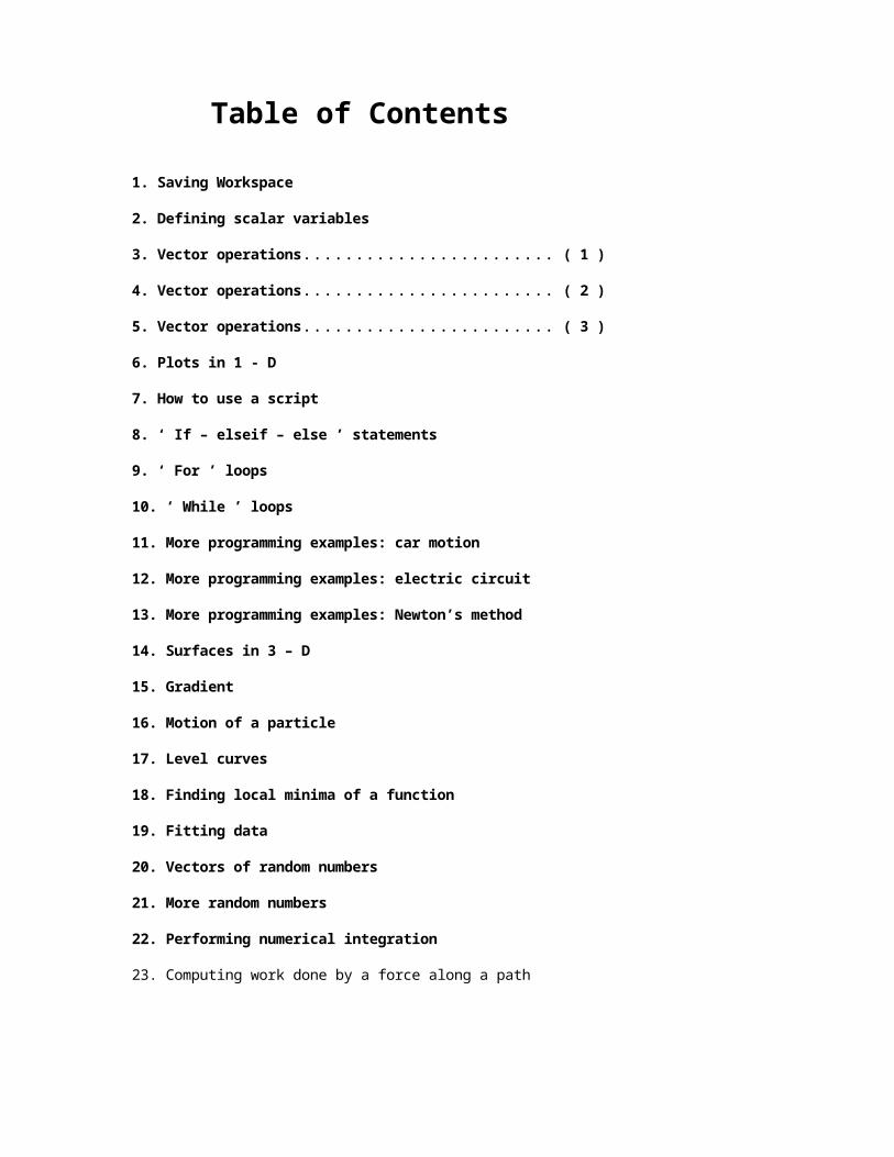
Table of Contents

1. Saving Workspace

2. Defining scalar variables

3. Vector operations ( 1 )

4. Vector operations ( 2 )

5. Vector operations ( 3 )

6. Plots in 1 - D

7. How to use a script

8. ‘ If – elseif – else ’ statements

9. ‘ For ’ loops

10. ‘ While ’ loops

11. More programming examples: car motion

12. More programming examples: electric circuit

13. More programming examples: Newton’s method

14. Surfaces in 3 – D

15. Gradient

16. Motion of a particle

17. Level curves

18. Finding local minima of a function

19. Fitting data

20. Vectors of random numbers

21. More random numbers

22. Performing numerical integration

23. Computing work done by a force along a path

Getting started1. Saving Workspace

Commands : diary Start saving commands in a filediary(‘filename’) Start saving commands in the file filenamediary off Stop the diary

The diary command allows saving all command window inputs and outputs (except graphics) in a separate file, which can be opened with most text editors (e.g. Microsoft Word) and printed.

Start the diary and save the file as mydiary. Compute the number of seconds in one year. Close the diary. Open the file mydiary using any text editor.

SOLUTION

In the Command Window : >> diary(‘mydiary’)>> 60*60*24*365ans =31536000

>> diary off

In Microsoft Word :

60*60*24*365ans =31536000diary off

Hint: MATLAB workspace will be saved into a file named diary when no file name is specified.

Hint: If you need help with a specific MATLAB command, simply type help command name in the command window. Detailed information will be displayed with everything needed to use this command properly. If you don’t know the exact name of the command, type lookfor keyword, which returns all the commands related to that keyword.

YOUR TURN

Start a new diary and call it newdiary. Compute the product of all the integers from 1 to 9. Close the diary. Open it with a text editor and print it.

2. Defining scalar variables

Commands : + - / * ^ ; Basic algebraic operationsclear Clear variables from the workspace% Insert a comment

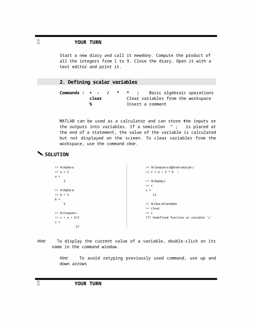
MATLAB can be used as a calculator and can store the inputs or the outputs into variables. If a semicolon “ ; ” is placed at the end of a statement, the value of the variable is calculated but not displayed on the screen. To clear variables from the workspace, use the command clear.

SOLUTION

>> % Define a>> a = 2a = 2

>> % Define b>> b = 5b = 5

>> % Compute c>> c = a + b^2c = 27

>> % Compute a different value for c>> c = a + 2 * b ;

>> % Display c>> cc = 12

>> % Clear all variables >> clear>> c??? Undefined function or variable 'c'

Hint: To display the current value of a variable, double-click on its name in the command window.

Hint: To avoid retyping previously used command, use up and down arrows

YOUR TURN

Set variable a to 12345679, variable b to 9, and assign your favorite number between 1 and 9 to c. Compute the product abc and display it on the screen. Clear all variables at the end.

3. Vector operations ( 1 )

Commands: linspace (x0, x1, N) Create an array of N equally spaced values between x0 and x1

x0 : Δx : x1 Create an array of values between x0 and x1 spaced by Δx

PART 1

Create the vector . Display each of the elements. Multiply the first and second elements. Change the third element to 4 and display the new vector on the screen.

SOLUTION

>> V = [1 2 3]V = 1 2 3

>> V (1)ans = 1

>> V (2)

ans = 2

>> V (3)ans = 3

>> x = V (1)*V (2)

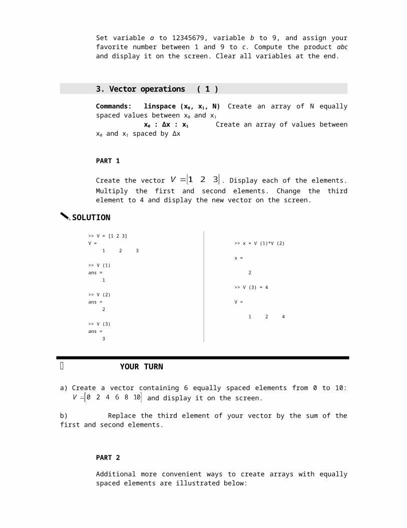
x =

2

>> V (3) = 4

V =

1 2 4

YOUR TURN

a) Create a vector containing 6 equally spaced elements from 0 to 10: and display it on the screen.

b) Replace the third element of your vector by the sum of the first and second elements.

PART 2

Additional more convenient ways to create arrays with equally spaced elements are illustrated below:

>> V = linspace ( 0 , 10 , 6 )V = 0 2 4 6 8 10

>> W = 0 : 2 : 10W =

0 2 4 6 8 10

YOUR TURNc) Create a vector containing elements spaced by 0.2 between 1 and 2.

d) Create a vector containing 10 equally spaced elements between 1.5 and 2.

Hint: You can check the dimension of an array in the command window using the size command.

4. Vector operations ( 2 )

Commands : .* ./ .^ element by element algebraic operations

Define two vectors and . Multiply x and y element by element. Compute the squares of the elements of x.

SOLUTION

>> % Define x and y

>> x=[1 -2 5 3];>> y=[4 1 0 -1];

>> % Compute z

>> z = x . * y

z =

4 -2 0 -3

>> % Compute the squares of the elements of x >> x . ^ 2

ans =

1 4 25 9

Hint: A period is needed for element-by-element operations with arrays in front of *, / , and ^ . A period is NOT needed in front of + and - .

YOUR TURN

Divide y by x element by element. Display the result.

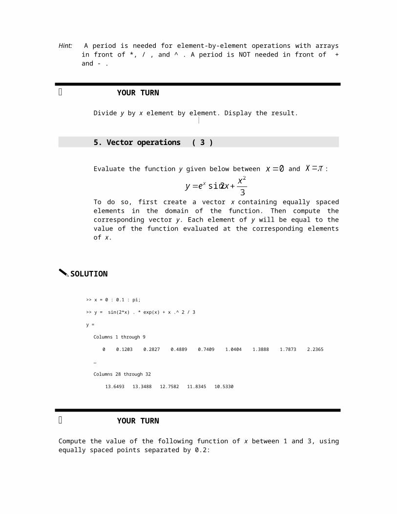
5. Vector operations ( 3 )

Evaluate the function y given below between and :

To do so, first create a vector x containing equally spaced elements in the domain of the function. Then compute the corresponding vector y. Each element of y will be equal to the value of the function evaluated at the corresponding elements of x.

SOLUTION

>> x = 0 : 0.1 : pi;

>> y = sin(2*x) . * exp(x) + x .^ 2 / 3

y =

Columns 1 through 9

0 0.1203 0.2827 0.4889 0.7409 1.0404 1.3888 1.7873 2.2365

…

Columns 28 through 32

13.6493 13.3488 12.7582 11.8345 10.5330

YOUR TURN

Compute the value of the following function of x between 1 and 3, using equally spaced points separated by 0.2:

6. Plots in 1 - D

Commands : plot Create a scatter/line plot in 1-D title Add a title to the current figure

xlabel, ylabel Add x and y labels to the current figurelegend Add a legend to the current figurehold on / hold off Plot multiple curves in the same figuresubplot Make several plots in the same window

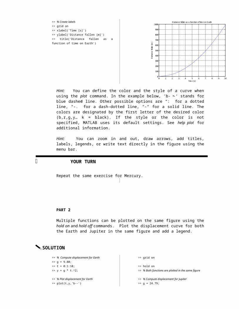
The displacement of an object falling under the force of gravity is given by:

where g is the acceleration of gravity [m/s2], y is the distance traveled [m], and t is time [s].

The following table gives the values of g for three different planets:

PART 1

Plot the distance fallen as a function of time near the surface of the Earth between 0 and 10 seconds, with an increment of 1 second. Add a title and x and y labels.

SOLUTION

>> % Define time values>> t = 0:1:10;

>> % Define acceleration of gravity >> g = 9.80;

>> % Compute displacement y>> y = g * t.^2;

>> % Plot>> plot(t,y,'b--')

>> % Create labels>> grid on>> xlabel('Time [s]')>> ylabel('Distance fallen [m]')>> title('Distance fallen as a function of time on Earth')

0 1 2 3 4 5 6 7 8 9 100

100

200

300

400

500

600

700

800

900

1000

Time [s]

Dis

tanc

e fa

llen

[m]

Distance fallen as a function of time on Earth

Planet

g

Earth

9.80 m/s2

Jupiter

24.79 m/s2

Mercury

3.72 m/s2

Hint: You can define the color and the style of a curve when using the plot command. In the example below, ‘b- -‘ stands for blue dashed line. Other possible options are “:” for a dotted line, “-.” for a dash-dotted line, “-“ for a solid line. The colors are designated by the first letter of the desired color (b,r,g,y… k = black). If the style or the color is not specified, MATLAB uses its default settings. See help plot for additional information.

Hint: You can zoom in and out, draw arrows, add titles, labels, legends, or write text directly in the figure using the menu bar.

YOUR TURN

Repeat the same exercise for Mercury.

PART 2

Multiple functions can be plotted on the same figure using the hold on and hold off commands. Plot the displacement curve for both the Earth and Jupiter in the same figure and add a legend.

SOLUTION

>> % Compute displacement for Earth>> g = 9.80;>> t = 0:1:10;>> y = g * t.^2;

>> % Plot displacement for Earth>> plot(t,y,'b--')>> grid on

>> hold on>> % Both functions are plotted in the same figure

>> % Compute displacement for Jupiter>> g = 24.79;>> y = g * t.^2;

>> % Plot displacement for Jupiter>> plot(t,y,'r-')

>> % Create labels>> title('Distance fallen as a function of time')>> xlabel('Time [s]')

>> ylabel('Distance fallen [m]')>> % Add a legend>> legend('Earth','Jupiter')

>> % End of the hold command>> hold off

0 1 2 3 4 5 6 7 8 9 100

500

1000

1500

2000

2500Distance fallen as a function of time

Time [s]

Dis

tanc

e fa

llen

[m]

EarthJupiter

YOUR TURN

Plot all three curves for the three planets in the same figure. Use different styles for each of the planets and include a legend

PART 3

The three curves can also be plotted on the same figure in three different plots using the subplot command. Plot the curves for Earth and Jupiter using subplot.

SOLUTION

>> % Compute displacement for Earth>> t = 0:1:10;>> g = 9.80;>> y = g*t.^2;

>> % Plot>> subplot (2,1,1)>> plot (t,y,'b--')>> xlabel ('Time [s]')>> ylabel ('Distance fallen [m]')>> title ('Distance fallen as a function of time on Earth')>> grid on

>> % Define displacement for Jupiter>> g=24.79;>> y = g*t.^2;

>> % Plot>> subplot(2,1,2)

>> plot(t,y,'r-')>> xlabel('Time [s]')>> ylabel('Distance fallen [m]')>> title('Distance fallen as a function of time on Jupiter')>> grid on

0 1 2 3 4 5 6 7 8 9 100

200

400

600

800

1000

Time [s]

Dis

tanc

e fa

llen

[m]

Distance fallen as a function of time on Earth

0 1 2 3 4 5 6 7 8 9 100

500

1000

1500

2000

2500

Time [s]

Dis

tanc

e fa

llen

[m]

Distance fallen as a function of time on Jupiter

YOUR TURN

Using subplot, create three different displacement plots in the same window corresponding to each of the three planets.

Programming

7. How to use a script

Commands : clear Clear all variables close Close the current figure

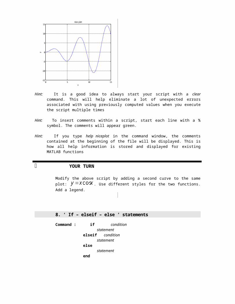
Open a new script (or .m) file.

Plot the function between 0 and 15 using 1000 points. Include labels and a title.

Save your file as niceplot.m. In the command window, select the appropriate directory and execute the script by typing niceplot in the command window

SOLUTION

Open new .m fileType commands

% Creating a nice plot

% Clear all the variablesclear% Close current windowclose

% Defining the function x = linspace ( 0 , 15 , 1000 );y = sin(x) .* x;

% Plotting y plot ( x , y )grid ontitle ( ‘nice plot’ )xlabel ( ‘x’ )ylabel ( ‘y’ )

Save file as niceplot.mExecute script :

>> niceplot

0 5 10 15-15

-10

-5

0

5

10

15nice plot

x

y

Hint: It is a good idea to always start your script with a clear command. This will help eliminate a lot of unexpected errors associated with using previously computed values when you execute the script multiple times

Hint: To insert comments within a script, start each line with a % symbol. The comments will appear green.

Hint: If you type help niceplot in the command window, the comments contained at the beginning of the file will be displayed. This is how all help information is stored and displayed for existing MATLAB functions

YOUR TURN

Modify the above script by adding a second curve to the same plot: . Use different styles for the two functions. Add a legend.

8. ‘ If – elseif – else ’ statements

Command : if conditionstatement

elseif conditionstatement

elsestatement

end

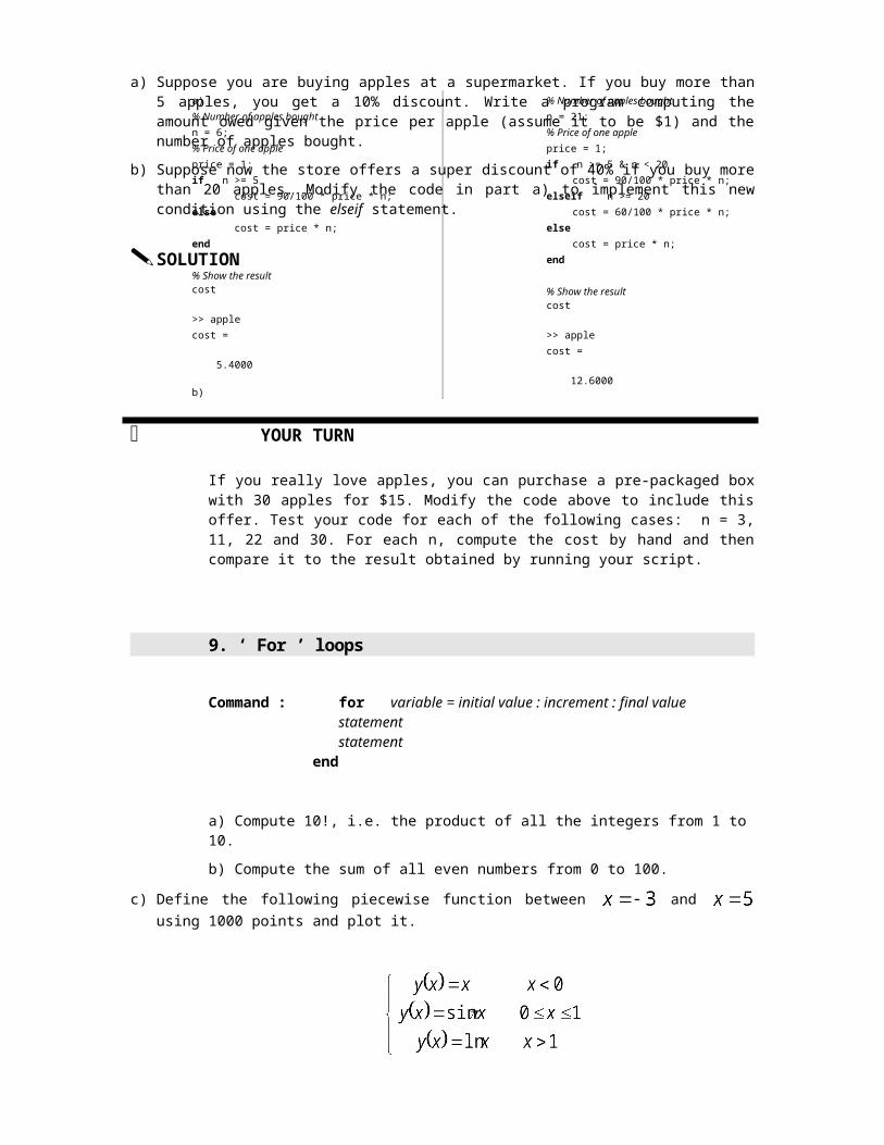
a) Suppose you are buying apples at a supermarket. If you buy more than 5 apples, you get a 10% discount. Write a program computing the amount owed given the price per apple (assume it to be $1) and the number of apples bought.

b) Suppose now the store offers a super discount of 40% if you buy more than 20 apples. Modify the code in part a) to implement this new condition using the elseif statement.

SOLUTION

a)% Number of apples boughtn = 6;% Price of one appleprice = 1;if n >= 5 cost = 90/100 * price * n;else cost = price * n;end

% Show the resultcost

>> applecost =

5.4000

b)

% Number of apples boughtn = 21;% Price of one appleprice = 1;if n >= 5 & n < 20 cost = 90/100 * price * n;elseif n >= 20 cost = 60/100 * price * n;else cost = price * n;end

% Show the resultcost

>> applecost =

12.6000

YOUR TURN

If you really love apples, you can purchase a pre-packaged box with 30 apples for $15. Modify the code above to include this offer. Test your code for each of the following cases: n

= 3, 11, 22 and 30. For each n, compute the cost by hand and then compare it to the result obtained by running your script.

9. ‘ For ’ loops

Command : for variable = initial value : increment : final valuestatementstatement

end

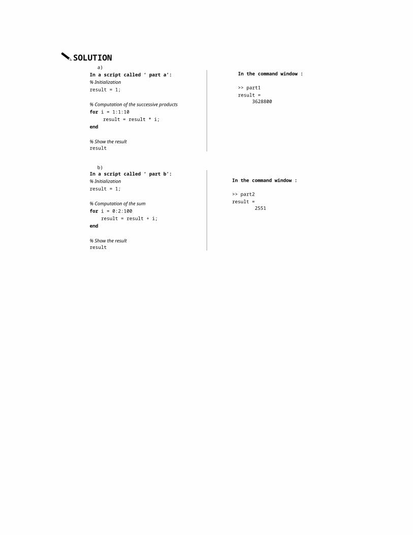
a) Compute 10!, i.e. the product of all the integers from 1 to 10.

b) Compute the sum of all even numbers from 0 to 100.

c) Define the following piecewise function between and using 1000 points and plot it.

SOLUTION a)

In a script called ‘ part a’: % Initializationresult = 1;

% Computation of the successive productsfor i = 1:1:10 result = result * i;end

% Show the resultresult

In the command window :

>> part1result = 3628800

b)In a script called ‘ part b’:% Initializationresult = 1;

% Computation of the sumfor i = 0:2:100 result = result + i;end

% Show the resultresult

In the command window :

>> part2result = 2551

c)

In a script called ‘ part c’:% Define vector xx = linspace(-3,5,1000);% Test each value of x and compute the % appropriate value for y

for i = 1:length(x)

if x(i) < 0 y(i) = x(i); elseif x(i)>1 y(i) = log(x(i)); else y(i) = sin (pi * x(i)); end

end

% Plot y as a function of xplot(x,y)

-3 -2 -1 0 1 2 3 4 5-3

-2.5

-2

-1.5

-1

-0.5

0

0.5

1

1.5

2

x

y

YOUR TURN

a) Write a script to compute the sum of all components of a vector. Your script should work regardless of the size of the vector. Test your script with using the following vector:

.

b) Define and plot the function for x ranging between –1 and 1, with x coordinates spaced by 0.05.

10. ‘ While ’ loops

Command : while condition statement

end

abs (x) returns the absolute value of xsqrt (x) returns the square root of x

If x is an approximate value of the square root of a number a, then is generally

a better approximation. For example, with a = 2, starting with x = 1, we obtain the following

successive approximations: approaching in the limit the true value of

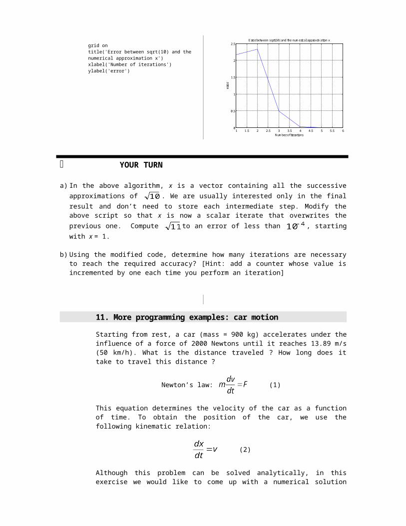
Using the above formula, write a script to compute iteratively the value of . At each step, compare your solution to the exact value of and stop your iteration when the difference between your solution and the exact one is less than . Start the iteration with the initial guess x = 1. Plot the absolute value of the error versus the current iteration number.

SOLUTION% Value of aa = 10;

% First guess for the square root of ax(1) = 1;

i = 1;% If the error is greater than 10^-4, continue iteratingwhile abs (x (i) – sqrt (10) ) >= 10^-4 i = i + 1; x ( i ) = 1/2 * (x (i-1) + a / x (i-1));end

% Show the resultx ( i )plot ( abs ( x-sqrt(10) ) )

grid on

title('Error between sqrt(10) and the numerical approximation x')xlabel('Number of iterations')ylabel('error')

1 1.5 2 2.5 3 3.5 4 4.5 5 5.5 60

0.5

1

1.5

2

2.5Error between sqrt(10) and the numerical approximation x

Number of iterations

erro

r

YOUR TURN

a) In the above algorithm, x is a vector containing all the successive approximations of . We are usually interested only in the final result and don’t need to store each intermediate step. Modify the above script so that x is now a scalar iterate that overwrites the previous one. Compute to an error of less than , starting with x = 1.

b) Using the modified code, determine how many iterations are necessary to reach the required accuracy? [Hint: add a counter whose value is incremented by one each time you perform an iteration]

11. More programming examples: car motion

Starting from rest, a car (mass = 900 kg) accelerates under the influence of a force of 2000 Newtons until it reaches 13.89 m/s (50 km/h). What is the distance traveled ? How long does it take to travel this distance ?

Newton’s law: (1)

This equation determines the velocity of the car as a function of time. To obtain the position of the car, we use the following kinematic relation:

(2)

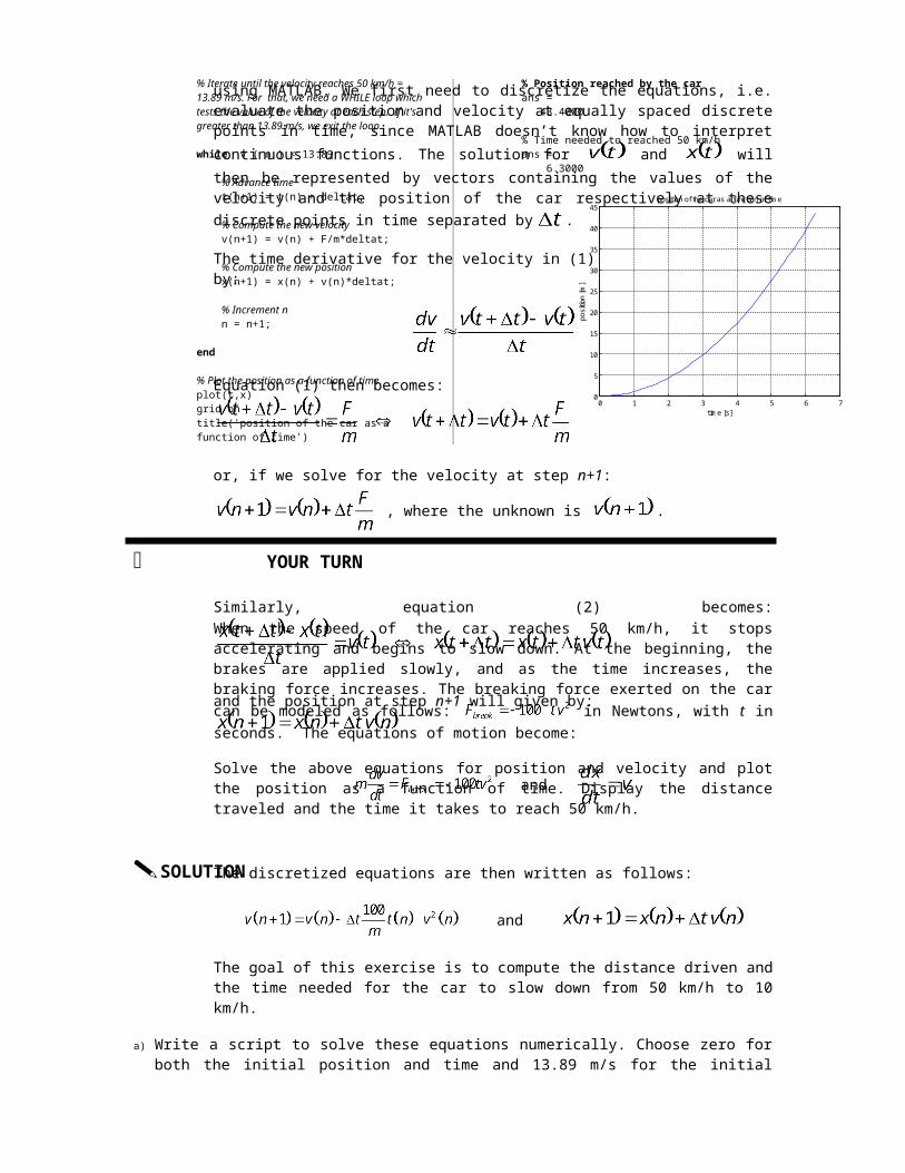
Although this problem can be solved analytically, in this exercise we would like to come up with a numerical solution using MATLAB. We first need to discretize the equations, i.e. evaluate the position and velocity at equally spaced discrete points in time, since MATLAB doesn’t know how to interpret continuous functions. The solution for and will then be represented by vectors containing the values of the velocity and the position of the car respectively at these discrete points in time separated by .

The time derivative for the velocity in (1) can be approximated by:

Equation (1) then becomes:

or, if we solve for the velocity at step n+1: , where the unknown is

.

Similarly, equation (2) becomes:

and the position at step n+1 will given by:

Solve the above equations for position and velocity and plot the position as a function of time. Display the distance traveled and the time it takes to reach 50 km/h.

SOLUTION

% Force applied to the car in NewtonsF = 2000;% Mass of the car in kgm = 900;% Time step in secondsdeltat = 0.1

% Initialization: at t=0, the car is at restt(1) = 0;v(1) = 0;x(1) = 0;

n = 1;% Iterate until the velocity reaches 50 km/h = 13.89 m/s. For that, we need a WHILE loop which tests the value of the velocity at each step. If it's greater than 13.89 m/s, we exit the loop.

while v ( n ) < 13.89 % Advance time t(n+1) = t(n) + deltat; % Compute the new velocity v(n+1) = v(n) + F/m*deltat; % Compute the new position x(n+1) = x(n) + v(n)*deltat; % Increment n n = n+1; end

% Plot the position as a function of timeplot(t,x)grid ontitle('position of the car as a function of time')xlabel('time [s]')

ylabel('position [m]')

% Display the position reached by the car (last element of the x vector) x(length(x))

% Time needed to go from 0 to 50 km/h (last element of the t vector)t(length(t))

In the command window:% Position reached by the carans = 43.4000

% Time needed to reached 50 km/hans = 6.3000

0 1 2 3 4 5 6 70

5

10

15

20

25

30

35

40

45position of the car as a function of time

time [s]

posi

tion

[m]

YOUR TURN

When the speed of the car reaches 50 km/h, it stops accelerating and begins to slow down. At the beginning, the brakes are applied slowly, and as the time increases, the braking force increases. The breaking force exerted on the car can be modeled as follows:

in Newtons, with t in seconds. The equations of motion become:

and

The discretized equations are then written as follows:

and

The goal of this exercise is to compute the distance driven and the time needed for the car to slow down from 50 km/h to 10 km/h.

a) Write a script to solve these equations numerically. Choose zero for both the initial position and time and 13.89 m/s for the initial velocity. Use the same time step as in the above example. Stop the iteration when the velocity reaches 2.78 m/s (10 km/h).

b) Plot the position and velocity as a function of time in the same figure, using subplot. Add a title, labels, and a grid.

c) Determine the time and the distance traveled to slow down to 10 km/h.

12. More programming examples: electric circuit

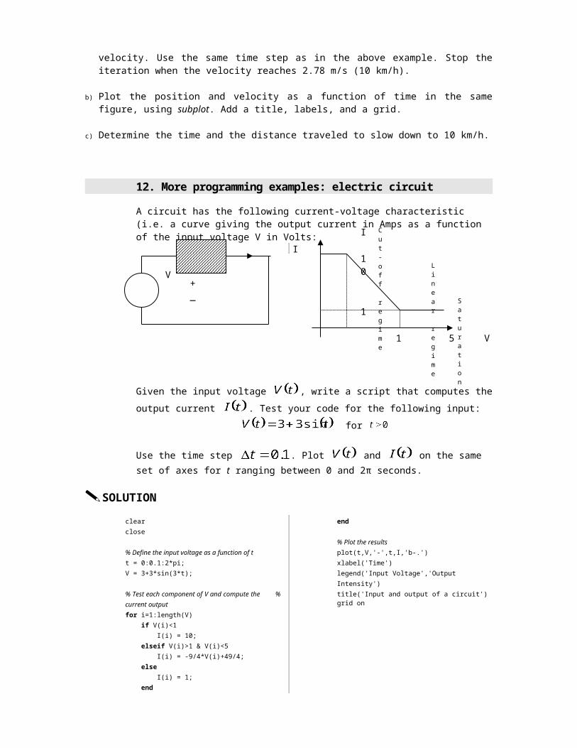
A circuit has the following current-voltage characteristic (i.e. a curve giving the output current in Amps as a function of the input voltage V in Volts:

Given the input voltage , write a script that computes the output current . Test your code for the following input:

for

Use the time step . Plot and on the same set of axes for t ranging between 0 and 2π seconds.

SOLUTION

clearclose

% Define the input voltage as a function of tt = 0:0.1:2*pi;V = 3+3*sin(3*t);

% Test each component of V and compute the % current outputfor i=1:length(V) if V(i)<1 I(i) = 10; elseif V(i)>1 & V(i)<5 I(i) = -9/4*V(i)+49/4; else I(i) = 1; endend

% Plot the results

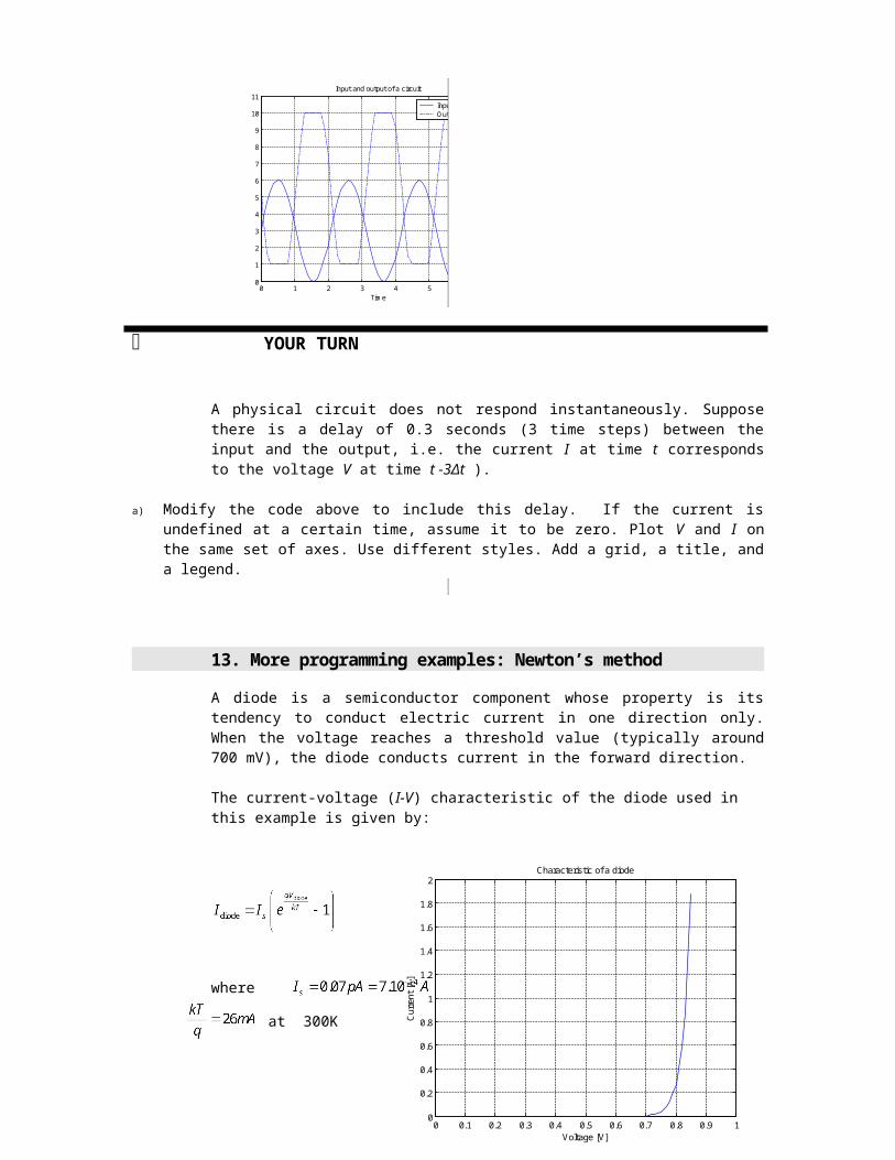
plot(t,V,'-',t,I,'b-.')xlabel('Time')legend('Input Voltage','Output Intensity')title('Input and output of a circuit')grid on

0 1 2 3 4 5 6 70

1

2

3

4

5

6

7

8

9

10

11

Time

Input and output of a circuit

Input VoltageOutput Intensity

YOUR TURN

V

I

V

I

10

1

1 5

Cut-off regime

Linear regime

Saturation

+_

A physical circuit does not respond instantaneously. Suppose there is a delay of 0.3 seconds (3 time steps) between the input and the output, i.e. the current I at time t corresponds to the voltage V at time t -3Δt ).

a) Modify the code above to include this delay. If the current is undefined at a certain time, assume it to be zero. Plot V and I on the same set of axes. Use different styles. Add a grid, a title, and a legend.

13. More programming examples: Newton’s method

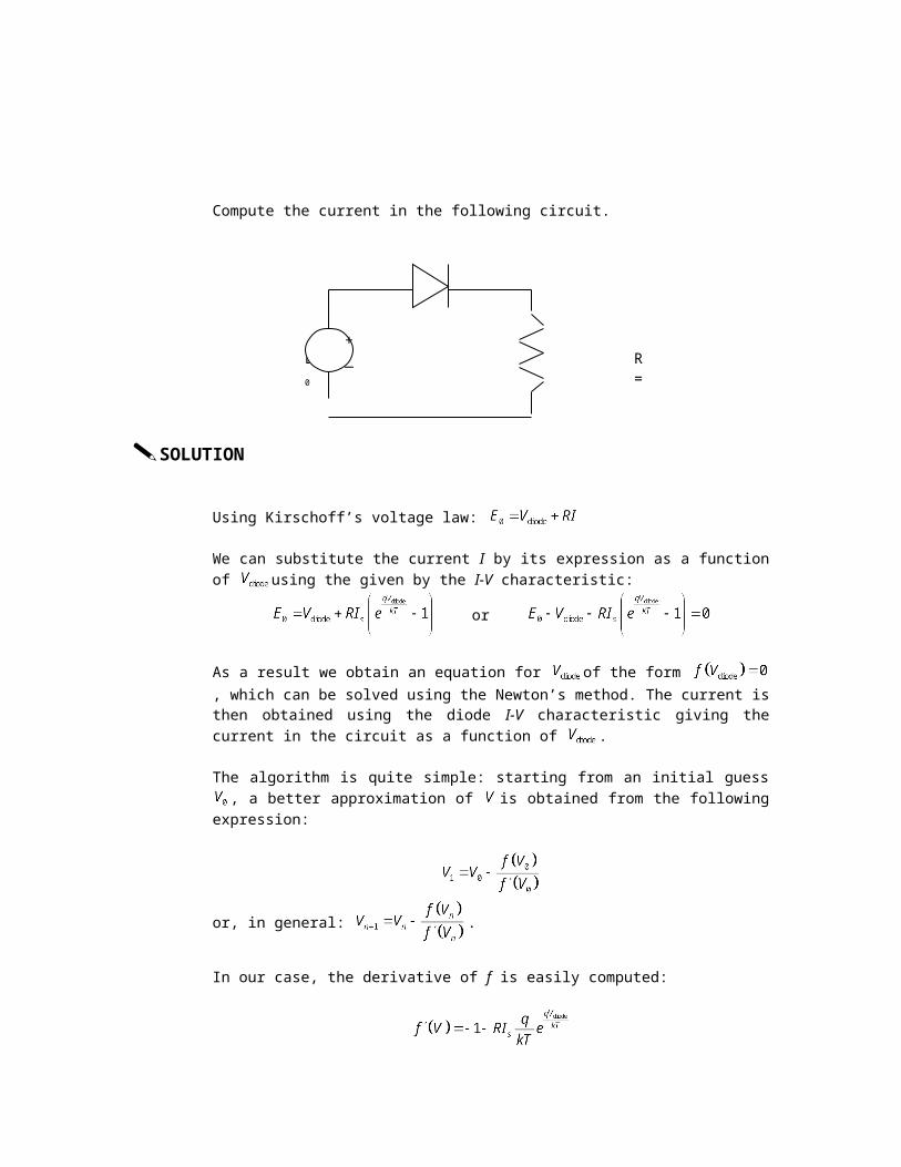
A diode is a semiconductor component whose property is its tendency to conduct electric current in one direction only. When the voltage reaches a threshold value (typically around 700 mV), the diode conducts current in the forward direction.

The current-voltage (I-V) characteristic of the diode used in this example is given by:

where

at 300K

Compute the current in the following circuit.

SOLUTION

Using Kirschoff’s voltage law:

We can substitute the current I by its expression as a function of using the given by the I-V characteristic:

or

0 0.1 0.2 0.3 0.4 0.5 0.6 0.7 0.8 0.9 10

0.2

0.4

0.6

0.8

1

1.2

1.4

1.6

1.8

2Characteristic of a diode

Voltage [V]

Cur

rent

[A]

E0 =

R = 20

+_

As a result we obtain an equation for of the form , which can be solved using the Newton’s method. The current is then obtained using the diode I-V characteristic giving the current in the circuit as a function of .

The algorithm is quite simple: starting from an initial guess , a better approximation of is obtained from the following expression:

or, in general: .

In our case, the derivative of f is easily computed:

Perform several iterations of the Newton’s method using the for loop. Find the diode voltage and the current in the circuit using 20 iterations.

In a script:

clear

% Parameters of the problemE0 = 3; % Input voltageIs = 7*10^-14; % Value of IsR = 200; % Value of the resistorC = 0.026; % Value of KT/q

% Initial guess for VdiodeVdiode = 1;

% Iterationsfor i = 1:20 % computation of the derivative of f evaluated at Vdiode fprime = -1 - Is * R / C * exp( Vdiode/C ); % computation of f evaluated at Vdiode

f = E0 - Vdiode - Is * R * ( exp( Vdiode/C ) - 1); % New value of VdiodeVdiode = Vdiode - f/fprime;end

% Display solution% VdiodeVdiode% Current in the circuitI = Is*(exp( Vdiode/C ) - 1)

In the command window:

>> newton

Vdiode = 0.6718I = 0.0116

YOUR TURN

A for loop was used in the above script to perform the Newton’s iteration. The iteration was terminated after a specified number of loops. In this case, we have performed a certain number of iterations without concerning ourselves with the accuracy of the computed solution. A more efficient approach would be to test for convergence and stop the iteration when the required level of accuracy has been achieved. This can be done using a while loop. The convergence criterion often used is the difference between the solutions obtained in two

successive iterations. The loop is terminated when the difference is below a specified threshold value.

a) Rewrite the above script using a while loop. Terminate the iteration when the absolute value of the difference between any two successive iterates for is less than 10-6. Note: you’ll have to store the old value of before computing the new one.

b) How many iterations were required to achieve the specified accuracy?

14. Surfaces in 3 – D

Command : meshgrid Create a two-dimensional grid of coordinate valuessurface Create a 3D surface on the domain defined by meshgrid

shading (‘interp’) Interpolate colormapcolorbar Add a colorbar

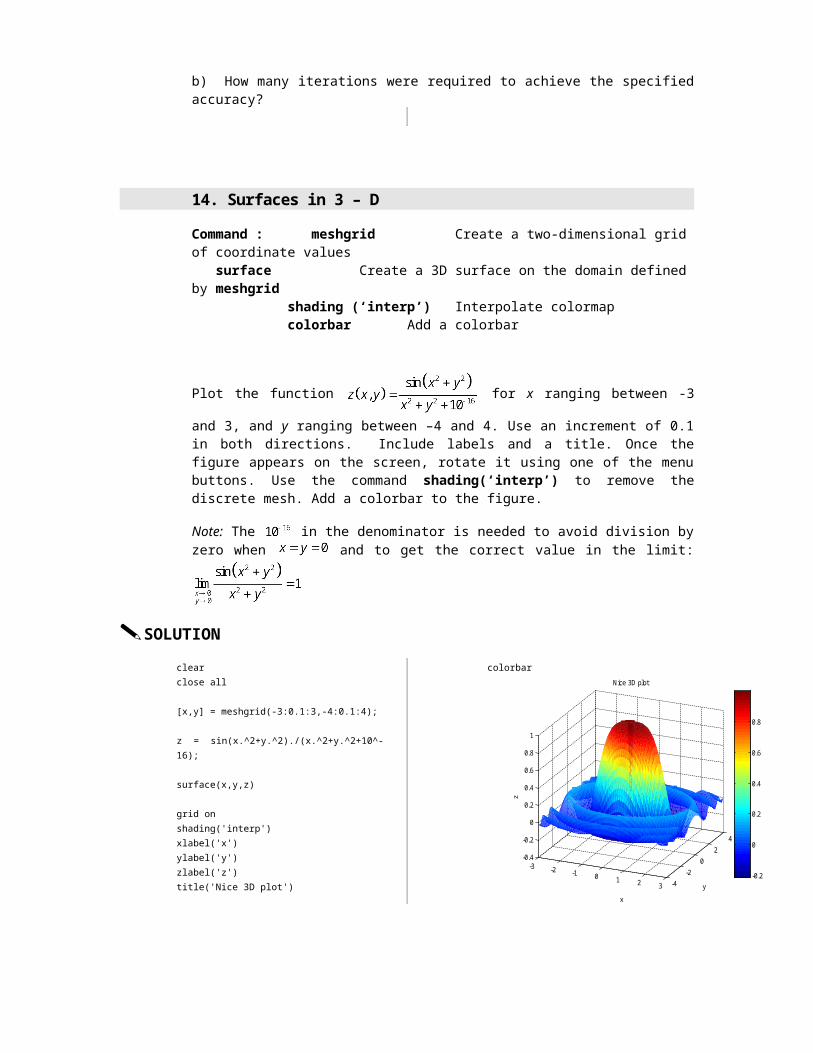
Plot the function for x ranging between -3 and 3, and y ranging

between –4 and 4. Use an increment of 0.1 in both directions. Include labels and a title. Once the figure appears on the screen, rotate it using one of the menu buttons. Use the command shading(‘interp’) to remove the discrete mesh. Add a colorbar to the figure.

Note: The in the denominator is needed to avoid division by zero when and

to get the correct value in the limit:

SOLUTION

clear close all

[x,y] = meshgrid(-3:0.1:3,-4:0.1:4);

z = sin(x.^2+y.^2)./(x.^2+y.^2+10^-16);

surface(x,y,z)

grid onshading('interp')xlabel('x')ylabel('y')zlabel('z')title('Nice 3D plot')colorbar

-3 -2 -1 0 1 2 3 -4-2

02

4

-0.4

-0.2

0

0.2

0.4

0.6

0.8

1

y

Nice 3D plot

x

z

-0.2

0

0.2

0.4

0.6

0.8

YOUR TURN

Plot the function

for x and y both ranging between and . Use an increment of 0.1. Do not use the shading option. Add labels and a title. Note: the plot you obtain represents a diffraction pattern produced by a small rectangular aperture illuminated by a monochromatic light beam. The function z represents the intensity of the light behind the aperture.

Hint: You can change the limits by selecting the arrow in the figure menu and double-clicking the figure itself. A window will appear in which you can modify the key parameters. Try to re-define the limits on z to go from 0 to 0.1 to better resolve surface features.

15. Gradient

Commands : gradient Computes the numerical derivative of a function

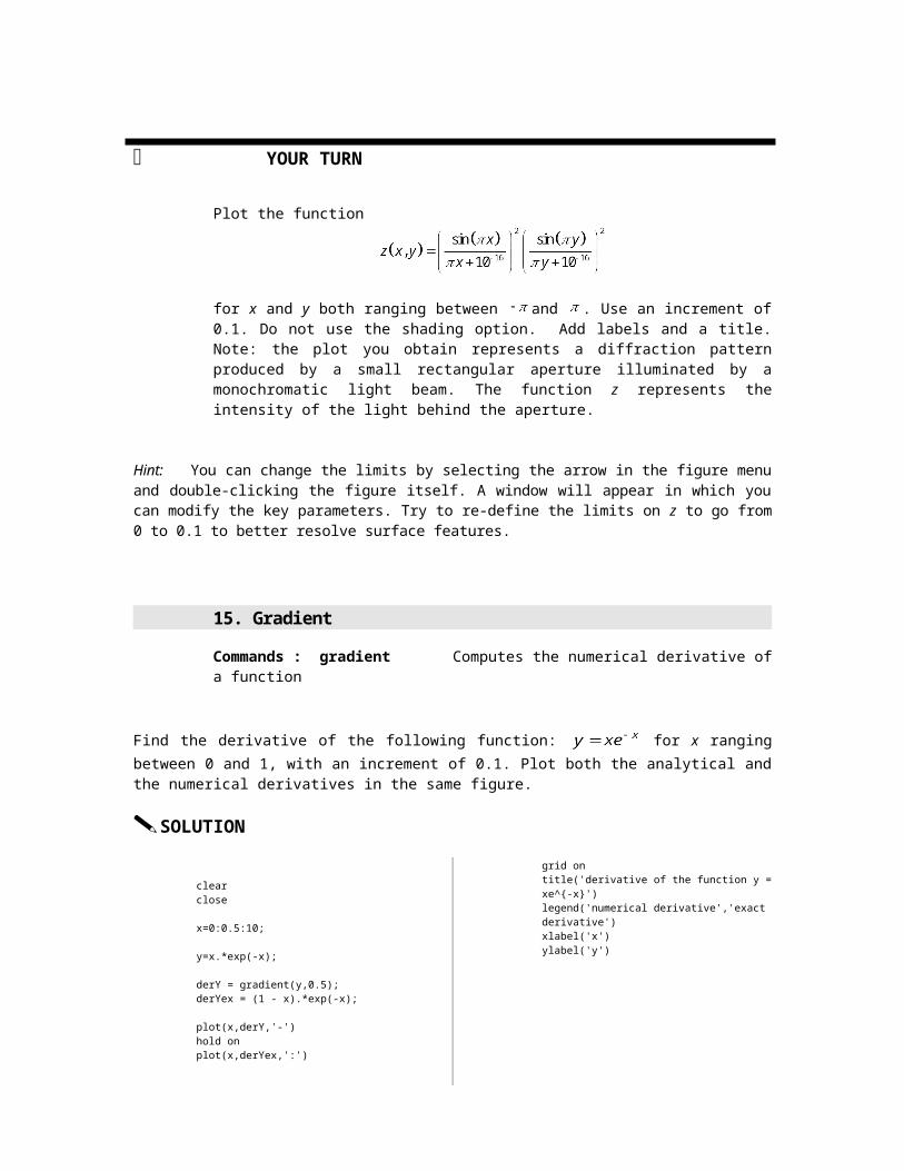
Find the derivative of the following function: for x ranging between 0 and 1, with an increment of 0.1. Plot both the analytical and the numerical derivatives in the same figure.

SOLUTION

clearclose

x=0:0.5:10;

y=x.*exp(-x);

derY = gradient(y,0.5);derYex = (1 - x).*exp(-x);

plot(x,derY,'-')hold onplot(x,derYex,':')

grid ontitle('derivative of the function y = xe^{-x}')legend('numerical derivative','exact derivative')xlabel('x')

ylabel('y')

0 1 2 3 4 5 6 7 8 9 10-0.2

0

0.2

0.4

0.6

0.8

1

1.2derivative of the function y = xe-x

x

y

numerical derivativeexact derivative

Hint: The spacing between points corresponds to the difference between the adjacent elements of vector x.

YOUR TURN

a) Compute analytically the derivative of the function

b) Using the gradient function, compute the derivative of the function in a) for x ranging between 0 and 1, with an increment of 0.1. Plot the analytical and the numerical derivatives in the same figure.

16. Motion of a particle

Command : plot3 Plot a curve in 3D

The motion of a particle in three dimensions is given by the following parametric equations:

for

a) plot the particle’s trajectory in 3D using the plot3 function

b) compute the velocity components , and the magnitude of the velocity vectorc) compute the acceleration components , and the magnitude of the acceleration

vectord) compute the components of the unit tangent vector e) compute the angle between the velocity vector and the acceleration vector

clear

% time vectordt = 0.1;t = 0:dt:2*pi;

% x, y and z vectorsx = cos(t);y = 2*sin(t);z = 0*t;

a)% plot trajectory in 3D plot3(x,y,z)grid onxlabel('x')ylabel('y')zlabel('z')

b)% Computation of the velocity components% Vx = dx/dtVx = gradient(x,dt);% Vy = dy/dtVy = gradient(y,dt);

% Speedspeed = sqrt(Vx.^2+Vy.^2);

c)% Computation of the acceleration components% Ax = dVx/dtAx = gradient(Vx,dt);% Ay = dVy/dtAy = gradient(Vy,dt);

% Accelerationacceleration = sqrt(Ax.^2+Ay.^2);

d)% Computation of the unit tangent vector components% Tx = Vx/|V|Tx = Vx./speed;% Ty = Vy/|V|Ty = Vy./speed;

e)% Computation of the angle between the velocity and acceleration vectors% cos(theta) = V.A/(|V||A|)theta = acos((Vx.*Ax+Vy.*Ay)./speed./acceleration);

-1-0.5

00.5

1

-2

-1

0

1

2-1

-0.5

0

0.5

1

xy

z

YOUR TURNThe equations of motion of the particle are given below:

for

a) Redo all 5 steps illustrated in the example aboveb) Verify that the magnitude of your tangent vector at is unity.c) Plot the velocity, acceleration and the angle between the velocity and the acceleration vectors

using the subplot command. Comment on the values obtained for the acceleration for t equal to 0 and 2π.

Hint: To create several figures, type figure in the command window. A new window will appear.

17. Level curves

Command : meshgrid Create two-dimensional arrays to be used by meshc meshc Plot a surface with level curves contour Plot level curves

shading(‘interp’) Remove mesh from a surface plotcolorbar Add a colorbar

Consider the following function :

a) Plot the function z for x ranging between 0 and 2, with an increment of 0.1 in both directions using the meshc command. This command will draw the three-dimensional surface along with a contour plot underneath.

b) Make a contour plot of the function above using the contour command. This will only display the level curves in a horizontal plane. Include labels and a title.

Hint: Using the contour command, you can specify the number of levels you would like to be displayed. The default number is 10.

SOLUTION

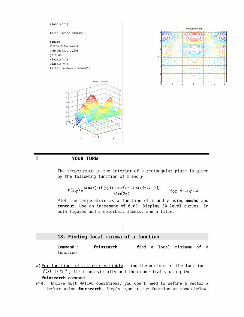
close allclear

% Define the grid[x,y]=meshgrid(0:0.1:2*pi);

% Define the function of two variablesz = y.*cos(x).*sin(2*y);

% Plot both surface and level curvesmeshc(x,y,z)grid onxlabel('x')ylabel('y')zlabel('z')

title('meshc command')

figure% Draw 20 level curvescontour(x,y,z,20)grid onxlabel('x')ylabel('y')title('contour command')

02

46

8

02

4

6

8-6

-4

-2

0

2

4

6

x

meshc command

y

z

0 1 2 3 4 5 60

1

2

3

4

5

6

x

y

contour command

YOUR TURN

The temperature in the interior of a rectangular plate is given by the following function of x and y:

for

Plot the temperature as a function of x and y using meshc and contour. Use an increment of 0.05. Display 30 level curves. In both figures add a colorbar, labels, and a title.

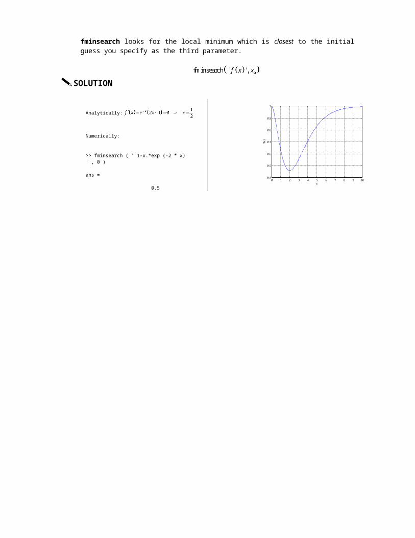
18. Finding local minima of a function

Command : fminsearch find a local minimum of a function

a) For functions of a single variable: find the minimum of the function , first analytically and then numerically using the fminsearch command.

Hint : Unlike most MATLAB operations, you don’t need to define a vector x before using fminsearch. Simply type in the function as shown below. fminsearch looks for the local minimum which is closest to the initial guess you specify as the third parameter.

SOLUTION

0 1 2 3 4 5 6 7 8 9 100.4

0.5

0.6

0.7

0.8

0.9

1

x

f(x)

b) For functions of several variables: find the minimum of the function over the

domain using the fminsearch command.

Follow these steps:- plot the function over the given domain to approximately locate the minimum.- use these approximate values of the coordinates as your initial guess

Hint: The syntax for functions of several variables is slightly different. Define . Then in

MATLAB, x and y will be represented by the two components: and , and the command becomes:

SOLUTION

>> % Plot the surface to visualize the minimum

>> [ x , y ] = meshgrid ( 0:0.1:pi , 0:0.1:pi ) ;>> f = cos(x.*y).*sin(x);>> surface(x,y,f);

>> % The minimum is around the point [ 1.5 2 ]

>> % Transform x and y in X(1) and X(2)

>> fminsearch( ' cos( x(1) * x(2)) * sin(x(1)) ',[1.5 2])

ans =

1.57082350280598 1.99997995837548 0

0.5

1

1.5

2

2.5

3

3.5

0

1

2

3

4-1

0

1

xy

f(x,y

)

YOUR TURN

Consider the following function of two variables:

a) Analytically find the minimum of this function

b) Plot the function on a suitably chosen domain to clearly see the minimum. Add a colorbar, labels, and a title

c) Using fminsearch, locate the minimum numerically

19. Fitting data

Command : polyfit find a polynomial that best fits a set of data

Reynolds number is a non-dimensional parameter frequently used in fluid mechanics:

where V is the characteristic velocity of the flowis the kinematic viscosity

L is the characteristic length scale of the flow (such as the length or the diameter of a body)

The Reynolds number indicates the relative importance of the viscous effects compared to the inertia effects. If the Reynolds number is low, viscous effects are predominant and if it’s large, viscosity can be ignored.

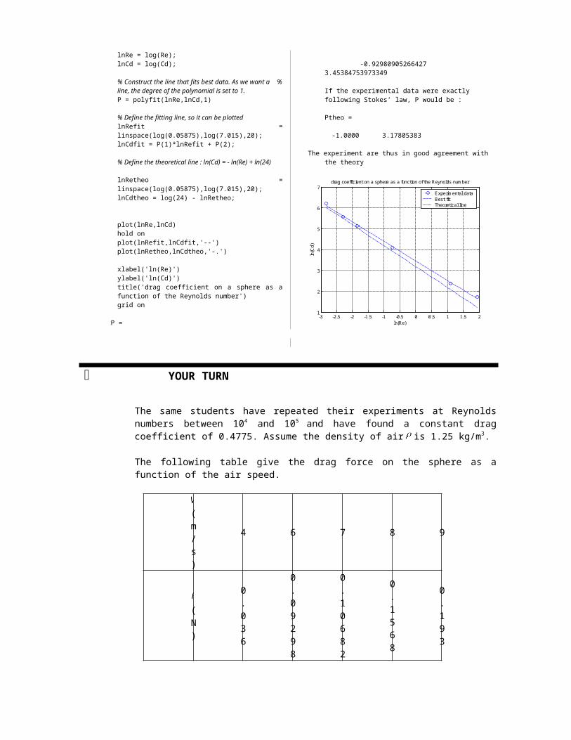
Let’s consider the force exerted on a sphere moving in the air. This drag force depends on the viscosity of the fluid, the velocity of the sphere and its dimension. Therefore, it is directly related to the Reynolds number. The drag force can be expressed as follows:

where is the density of air is the radius of the sphere is the velocity of the sphere is drag coefficient (non-dimensional)

In 1851 Stokes had demonstrated that the drag coefficient at low Reynolds numbers was inversely proportional to Re:

(low ) (1)

A group of students have measured this coefficient for a sphere of radius r in a wind tunnel. Here are their results. Confirm that the data satisfies the Stokes’ law.

Taking the logarithm of equation (1), we obtain:

(2)

To check whether the Stokes’ law is satisfied, we can plot versus and see whether the data points fall along a straight line. Follow these steps:

a) Create two vectors containing the logarithm of the experimental data and

b) Find the line that fits best these points. Display its coefficients on the screen and compare them with the theoretical result.

c) In the same figure plot the experimental data, the best fit line, and the theoretical line. Add a legend.

0.05875

0.1003

0.1585

0.4786

3.020

492

256 169.8

58.88

10.86

Hint: The polyfit command finds a polynomial of a specified order that best fits the given data. In this example, we want to see if the experimental data falls along a straight line. We therefore choose 1 as the degree of the polynomial.

Hint: The polyfit command returns a vector containing the coefficients of the polynomial: corresponding to

Hint: To suppress the line connecting the experimental data points, select the big arrow in the figure’s menu and double-click on the line. A property editor window will appear. Change the line style to ‘no line’ and choose circles for the marker style.

SOLUTIONclose allclear all

% Experimental dataRe = [0.05875 0.1003 0.1585 0.4786 3.020 7.015];Cd = [492 256.2 169.8 58.88 10.86 5.5623];

% Take the logarithm of these datalnRe = log(Re);lnCd = log(Cd);

% Construct the line that fits best data. As we want a % line, the degree of the polynomial is set to 1.P = polyfit(lnRe,lnCd,1)

% Define the fitting line, so it can be plottedlnRefit = linspace(log(0.05875),log(7.015),20);lnCdfit = P(1)*lnRefit + P(2);

% Define the theoretical line : ln(Cd) = - ln(Re) + ln(24)

lnRetheo = linspace(log(0.05875),log(7.015),20);lnCdtheo = log(24) - lnRetheo;

plot(lnRe,lnCd)hold on plot(lnRefit,lnCdfit,'--')plot(lnRetheo,lnCdtheo,'-.')

xlabel('ln(Re)')ylabel('ln(Cd)')title('drag coefficient on a sphere as a function of the Reynolds number')grid on

P =

-0.92980905266427 3.45384753973349

If the experimental data were exactly following Stokes’ law, P would be :

Ptheo =

-1.0000 3.17805383

The experiment are thus in good agreement with the theory

-3 -2.5 -2 -1.5 -1 -0.5 0 0.5 1 1.5 21

2

3

4

5

6

7

ln(Re)

ln(C

d)

drag coefficient on a sphere as a function of the Reynolds number

Experimental dataBest fitTheoretical line

YOUR TURN

The same students have repeated their experiments at Reynolds numbers between 104 and 105

and have found a constant drag coefficient of 0.4775. Assume the density of air is 1.25 kg/m3.

The following table give the drag force on the sphere as a function of the air speed.

(m/s)

4 6 7 8 9

(N)

0.036

0.09298

0.10682

0.1568

0.193

Find the radius of the sphere used in the experiments. Follow these steps:

a) In the definition of the drag force:

the group is now a constant, since the drag coefficient is assumed to be constant. That means

that the plot of versus should be close to a straight line. Using polyfit, find an equation of a line that best fits the data given in the table

b) Using the results in part a) extract the value of

c) Using the numerical values provided, estimate the radius of the sphere

20. Vectors of random numbers

Command : randn generate a vector whose components are chosen at randomhist plot a histogram

At the assembly line of a big aircraft company, bolts are stored in boxes containing 1000 parts each. The bolts are supposed to have a nominal diameter of 5 millimetres. But due to the uncertainty in the manufacturing process, some turn out to be larger and some turn out to be smaller than nominal.

a) Create a random vector whose components are the diameters of each bolt in a box using the randn command. The syntax of the randn command is as follows: randn ( M , N ) * A + B, where:

- M and N determine the size of the output vector, i.e. the number of random values generated. M corresponds to the number of rows and N to the number of columns. In our example, we want random diameters for 1000 bolts, so the output will be a vector with M = 1000 and N = 1

- A (called standard deviation) is related to the uncertainty in the diameter of the bolts. Here, A = 0.25 mm. This means that about 67% of the bolts have diameters within 0.25 mm of the nominal diameter.

- B is the nominal diameter of the bolts. Here, B = 5 mm

b) Plot a histogram showing the number of bolts as a function of their diameter

SOLUTIONa)

>> x = randn(1000,1) * 0.25 + 5;

b)

>> hist(x,30)>> title(‘Bolts contained in a box’)>> xlabel(‘Diameter in mm’)>> ylabel(‘Number of bolts’)

4.2 4.4 4.6 4.8 5 5.2 5.4 5.6 5.8 60

10

20

30

40

50

60

70

80

90

Diameter in mm

Num

ber o

f bol

ts

Bolts contained in a box

Hint : The hist command takes the vector generated by the randn command as input and counts the number of bolts having a diameter within a certain range (a bin). The number of bins is defined by the second parameter.

YOUR TURN

On the same assembly line, nuts are produced in boxes containing 5000 parts each. All nuts have a nominal diameter of 5.5 mm, however, the nuts in each box have been machined to different tolerances. Using subplot, plot the distributions of nuts as a function of their size for each of the four boxes for which the standard deviations are respectively A=0.45 mm, 0.50 mm, 0.55 mm and 60 mm.

21. More random numbers

Command : mean Compute the average of the components of a vectorstem Create a stem plot

Highway patrol uses a radar to measure the speed of the cars on a freeway. The speed limit is 55 mph. The officers pull over all cars whose speed is greater than 80 mph and write a ticket for $150 each. If 8000 vehicles are observed on the highway each day, on the average, how much money does the highway patrol collect each day ? Compute the average over one full year and assume A = 10 in the randn command.

SOLUTION

clear allclose all

% the average of the daily amount is done over a yearfor i = 1:365 % create a vector whose components are the speed of % each car taking the freewayx = randn(8000,1)*10 + 55; % Initialize the amount collected each dayS(i) = 0; % test the speed of each vehicle. If it's greater than 80, add % 150 to S

for k = 1:length(x)

if x(k) > 80 S(i) = S(i) + 150; end

endend

% Compute the average of vector S containing the amount % collected each day during a yearSavg = mean(S)

% Plot the ammount of money collected each daystem(S)xlabel('days')ylabel('amount')

Savg =

7374.65753424658

0 50 100 150 200 250 300 350 4000

2000

4000

6000

8000

10000

12000

days

amou

nt

YOUR TURN

Modify the above script compute the average percentage of cars that have a speed of more than 10 mph over the speed limit. Compute your daily average over one year.

22. Performing numerical integration

Command : trapz Computes the integral of a function over a given domain using the trapezoidal method

Compute the integral of the function for using the trapezoidal method. Compare the result to the exact analytical solution.

SOLUTIONclear closex = linspace(0,1,100)y = x.^2+x+1;

I = trapz(x,y)

I = 1.8333

Analytical result : I = 11/6 = 1.8333

YOUR TURN

a) Compute the following integral analytically:

b) Compute the same integral numerically using the trapz command. Use an increment of 0.01

c) Repeat part b), this time with an increment of 0.2. What’s your conclusion?

23. Computing work done by a force along a path

Our sun continuously radiates energy in the form of electromagnetic waves. When these waves are reflected off of or absorbed by a surface, pressure is applied. These infinitesimal forces cause a small acceleration, which, in the case of a satellite in orbit, modifies its path.

In this example, we’ll compute the work done by the force due to solar pressure acting on a satellite travelling in an elliptical orbit around the sun.

The force due to solar radiation can be written as where:

c is the speed of light. c = 3.108 m/sG is the incident solar power flux Watt/m2 A is the area of the spacecraft normal to the sun. The area is assumed to be constant A = 8

m2

unit vector directed from the spacecraft toward the sun

The orbit is planar and is given parametrically by the following equation: with

Find the work done by the force of solar radiation on the spacecraft over the following interval (

). Use the time step of .

SOLUTION

The work done by a force is computed using the following formula:

θ is the angle between the velocity vector and the force. Each component of the integral is computed separately. Then the integral is computed using the trapz command.

clear

% parametersG = 1350;A = 8;c = 3*10^8;

% definition of the orbitt = 0:0.001:pi/2;

% parameters of the ellipsea = 1.5*10^11;b = 1.3*10^11;

% definition of the parametric curvex = a*cos(t);y = b*sin(t);

% velocity of the spacecraftvelx = gradient(x,0.001);vely = gradient(y,0.001);

% magnitude of the velocityvelmag = sqrt(velx.^2+vely.^2);

% acceleration of the spacecraftaccx = gradient(velx,0.001);accy = gradient(vely,0.001);

% magnitude of the accelerationaccmag = sqrt(accx.^2+accy.^2);

% magnitude of the force due to solar radiationsf = -1/c*G*A;

% cosine of the angle between the force and the velocity % vectorcostheta = (velx.*accx+vely.*accy)./velmag./accmag;

% computation of the work done for t between 0 and piW = trapz(f*velmag.*costheta,t)

In the command window:

W =

7.1195e+005

YOUR TURN

Suppose that the spacecraft is now travelling in an orbit specified by the following parametric equation: where . Compute the

work done by solar radiation for