TEXAS BOARD OF WATER ENGINEERSDurwood Manford, Chairman

R. M. Dixon, MemberO. F. Dent, Member

.......•••~t. 0';·••

....tG"m~l'i~ ~ ~).lI: r••~~ w:. .. .. .e··i- .. .~.•......:.....

BULLETIN 6019

CONSUMPTIVE USE OF WATER

BY MAJOR CROPS IN TEXAS

November 1960

Reprinted July 1962

TEXAS BOARD OF WATER ENGINEERS

Durwood Manford, ChairmanR. M. Dixon, MemberO. F. Dent, Member

BULLETIN 6019

CONSUMPTIVE USE OF WATERBY MAJOR CROPS IN TEXAS

By

Louis L. McDanielsSurface Water Division

Texas Board of Water Engineers

November 1960

Reprinted July 1962

First Printing, November 1960

Second Printing, September 1961

Third Printing, July 1962

FORE\oJORD

Irrigation is practiced in different parts of Texas under various climatic

conditions. In the far western portion of the State, irrigation supplies almost

all of the water used by crops, while in the State's central region a signifi­

cant part of crop water requirements is derived from rainfall. Rainfall on the

eastern section of the State is sufficient for crop production most of the time,

but crop yields are often assured through the use of "insurance" irrigation dur­

ing infrequent critical dry periods of a few weeks duration.

This bulletin presents information on the water requirements of plants re­

gardless of whether this water is supplied by precipitation directly, or by

irrigation. The values given herein are not the amounts of water which are

to be applied to the land, or pumped from a water supply source, to achieve

agricultural production. Diversion amounts and field application volumes are

dependent upon the soil characteristics, canal losses, deep percolation, and

variations in times and amounts of rainfall. All these factors have to be

considered in determining the amounts of water to be diverted from a supply

for irrigation.

In order to determine the amount of irrigation water to be applied to the

land, it is necessary to know the water requirements of plants. This bulletin

presents the fundamental data of these water requirements of plants for use in

water resources planning. Subsequent publications will describe studies of

effective rainfall, irrigation efficiencies, and total diversion requirements.

TEXAS BOARD OF WATER ENGINEERS

.-:T

@O. F. Dent, Acting Chairman

November 23, 1960

TABLE OF CONTENTS

3~--~--~--~-~~--~~--~---=--~~--~----------~~-----------~-----

Page

ABSTRACT ---------------------------------------------------------------- 1

INTRODUCTION

ACKNOWLEDGEMENTS -------------------------------------------------------- 3

PERSONNEL -------------------------------------- --------- 4

DEFINITIONS ---------------------------------------- ------- 4

GENERAL DISCUSSION ------------------------------------------------------ 5

Divisions of the State --------------------------------------------- 5

Crops and Crop Groupings ------------------------------------------- 5

Crop Seasons ------------------------------------------------------- 6

Methods of Estimating Consumptive Use ------------------------------ 7

TBWE METHOD ------------------------------------------------------------- 8

Procedure of Computation ------------------------------------------- 8

BASIC DATA -------------------------------------------------------------- 10

Consumptive Use of Water by Crops ---------------------------------~ 10

Climatic Index ------------------------=---------------------------- 12

USE COEFFICIENTS ------------~~~--~~--~---~---------------~-------------- 12

TABULATIONS OF DATA -----~-~----------~---~~---~-~-------~--------------- 13

SELECTED BIBLIOGRAPHY ----~---~-------~---------~--------~--------------- 15

APPENDICES

Page

Appendix A - Descriptive Figures -~~-~---=--=---------------=------------A-I

Figure 1. Land resource divisions and irrigated areas ---------=--- A-3

2. Subdivision of irrigated areas -------------------------- A-4

3. Average-annual CLIMATIC-INDEX numbers forsubdivisions of irrigated areas ------------------------ A-5

4. Average planting date and length of growingseason of crops, by areas, in Texas -------------------- A-6

Appendix B - Tables of Experiment Data and Basic Relations -------------- B-1

Table 1. Basic Data ----------------------------=-----==---------- B-3

2. U. S, Weather Bureau First-Order Stations --------------- B-6

3. Climatic-Index Coefficients ------------~---------------- B-7

4. Climatic-Index Numbers ---------------------------------- B-8

Appendix C - Tables of Crop Consumptive Use ----------------------------- C-l

Average monthly and annual consumptive use, depth in inches, by areas,1946-55

Table 5. Alfalfa --=-------=-=-------==--------------------------- C-3

6. Corn -------------------------==---------------------=--- C-4

7. Cotton -------------------==----------------------------- C-5

8. Grains, Small ----------~----------=-------------------~-C-6

9. Orchards, Citrus ----~=--------=----=--------------------C-7

10. Orchards, Deciduous Fruit ---------~--------------------- C-7

11. Orchards, Pecan ---=----=---------=-----------=-=-------- C-7

12. Peanuts -----------------=------------------------------- C-8

13. Rice -----~----------==-~=------------------=------------C-8

14. Sorghum, Grain ------------------------------------------ C-9

15. Vegetables, Deep-Rooted ---=~---------=------------------C-lO

16. Vegetables, Shallow-Rooted ------------------------------ C-12

CON SUM P T I V E USE o F W ATE R

B Y M A J 0 R C R 0 P S

ABSTRACT

I N T E X A S

The study that resulted in the publication of this report was undertaken

in order to obtain fundamental data of the average amounts of water used con­

sumptively by agricultural crops, grown under favorable conditions including

a full water supply, and thus to fulfill partly the need for information re­

qUired for use in estimating the water requirements for irrigation.

The results published herein are estimates of average consumptive-use

amounts for 12 major crops and crop groupings, and are tabulated by months

for the respective length of growing season for each crop in each of 24 areas

of major production in the State.

A method for estimating consumptive use of water by crops was developed

by the Board of Water Engineers and used for the computation of the estimates

tabulated. The TBWE (Texas Board of Water Engineers) Method is a procedure

of relating experiment consumptive-use data to a composite relation of air

temperature, dew point temperature, wind movement, and solar radiation, to

obtain constant ratios or use coefficients for specific periods of time which

vary with respect to length of periods and stage of development of vegetal

growths.

The experiment data used were published consumptive-use amounts deter­

mined for crops grown in Texas, California, and Arizona. A composite relation

of the aforementioned climatic data was used to compute average values for all

areas of the state for the period 1946-55. These average values are called

CLlMATIC··INDEX numbers. These numbers were used in conjunction with the use

coefficients derived from the basic studies to compute estimates of monthly

consumptive use by specific crops in each area of the State.

The estimated consumptive-use amounts for specific crops, as computed by

this method, vary from place to place directly with the climatic-index number

only.

These data provide a basis for estimating the monthly water requirements

of plants on an average for production of agricultural crops in all areas of

the State; and thus provide a basis for estimating amounts of water required

from a source for irrigation when used with information describing amounts of

rainfall effective in supplying the water requirements of crops, soil moisture

available to crops, and losses involved with the distribution and application

of water for crop use.

CON SUM P T I V F. USE o F W ATE R

B Y M A J 0 R C R 0 P S

INTRODUCTION

I N T E X A S

The quantity of water required for the production of agricultural cropsunder irrigation must be known and inventoried in planning agricultural water­supply development.

This report presents estimates of average monthly depths of water usedconsumptively by major crops grown in Texas under conditions favorable to theproduction of agricultural crops, which includes a full water supply. Alsoincluded is a description of the TBWE (Texas Board of Water Engineers) methodwhich has been developed for and used in the computation of these estimates ofconsumptive use. The values which are given for the water used consumptivelyby each crop are based on reliable data available at this time and are recom­mended for interim use until more extensive and precise data are obtained.

The estimates appearing,in this report represent water requirements ofplants only and not the gross amounts of water necessary for diverBion from asurface or underground source to supply these plant reqUirements. Gross diver­sion reqUirements include consideration of many variable factors; such as canallosses, soil type, and method of water application, in addition to the waterrequirements of the plants. However, the water requirements of plants consti­tUte the fundamental data used to develop estimates of quantities of water tobe diverted for irrigation and are presented herein for this purpose.

ACKNOWLEDGEMENTS

All individuals and agencies, private and public, who have participatedin the observation and collection of basic data related to the subject of thisreport are to be commended for their contributions. Particularly acknowledge­ment for assistance in the collection of basic data and in the interpretationof that data directly related to this report is given to:

The late Mr. Richard D. W. Blood, State Climatologist, U. S. WeatherBureau, Austin, Texas

Mr. Dean W. Bloodgood, Retired Irrigation Engineer, Board of WaterEngineers, Austin, Texas and former Irrigation Engineer, U. S.Agricultural Research Service.

Dr. Morris E. Bloodworth, Professor of Soil Physics, Department ofAgronomy, A. & M. College of Texas.

- 3 -

U. S. Study Commission-Texas, Irrigation Collaboration Group: Mr.Paul T. Gillett, Chairman; and members from the U. S. Bureauof Recldmation, the U. S. Soil Conservation Service, the StateSoil Conservation Board, and the A. & M. College of Texas.

Mr. Tor J. Nordenson, Chief of Hydrologic Investigations Section,Hydrologic Services Division, U. S. Weather Bureau, Washington,D. C.

Mr. Robert V. Thurmond, Portland Cement Association, Austin, Texas.(Former Associate Planning Engineer, Texas Board of Water Engi­neers, and former Irrigation Engineer, Agricultural ExtensionService, A. & M. College of Texas.)

PERSONNEL

Preliminary planning and inception of a report on consumptive use of waterby, and irrigation requirements of, major crops grown under irrigation in Texasis credited to Robert V. Thurmond, working under the direction of McDonald D.Weinert, former Chief Engineer.

This report was prepared in Engineering Services, Board of Water Engineers,under the general supervision of John J. Vandertulip, Chief Engineer, and Seth D.Breeding, Chief Surface Water Engineer, by the Surface Water Division-Hydro­logic Section for use by the Planning Division and is based on a method forconsumptive-use determinations developed by Louis L. I1cDaniels, Acting Chiefof the Hydrologic Section.

The Data Processing Division, directed by Ivan M. Stout, assisted Mr.McDaniels by performing extensive computations and preparing listings in testsof several accepted methods in preliminary studies prior to the development ofthe objective TBWE method for computing consumptive use of water by major cropsgrown under favorable conditions of available water.

DEFINITIONS

Terms used in this report to describe the method employed and to identifythe relations and factors expressed are specifically defined, as follows:

CLIMATIC INDEX is a number expressing a composite relationof four climatic factors--air 'temperature, dew pointtemperature, wind movement, and solar radiation--asexpressed by plate 2 in the USWB (U, S. WeatherBureau) Technical Paper 37 1/ which in turn is basedon Equation 14 in the USWB Research Paper 38 £1.

11 Kohler, M. A., Nordenson, T. J., and Baker, D. R., 1959, EvaporationMaps for the United States: U. S. Weather Bureau Tech. Paper 37.

~I Kohler, H. A., Nordenson, T. J., and Fox, W. E., 1955, Evaporationfrom Pans and Lakes: U. S. Weather Bureau Research Paper 38.

- 4 -

E1uatio1 14 was derived from eVBporl~ion research studiesat Lake Hefner 1/ and at Lake Mead _ .

CONSUMPTIVE USE is the depth of water t in inches t removedfrom a vegetated area by evaporation of moisture fromsoil surface t by evaporation of intercepted water fromplant surfaces t by development of plant tlssue t and bytranspiration from vegetal growths. (Literature con­taining discussions of consumptive use of water byvegetation t evapotranspiration t and irrigation require­ments of agricuLtural crops is quite voluminous. Inlieu of many specific citations t a selected bibliogra­phy is presented at the end of this text.)

USE COEFFICIENT i's a number expressing the ratio of a CON­SUMPTIVE USE amount to a CLIMATIC INDEX.

The above terms are used in abbreviation t as follows: IC (CLIMATIC INDEX),UC (CONSUMPTIVE USE) t AND KU (USE COEFFICIENT).

GENERAL DISCUSSION

Divisions of the State

The State was divided into eight areas (see figure 1, appendix A, page A-:Hto form major land-resource divisions based on a complex characterized by simi­larities of vegetation, soil, climate, and water availability. These eightareas were further divided into 24 smaller areas (see figure 2 t appendix A,page A-4) on a similar but more refined basis.

Crops and Crop Groupings

The following basic crops and crop groups are those for which consumptive­Use amounts are presented:

AlfalfaCornCottonGrains, SmallOrchards, CitrusOrchards, Deciduous Fruit

Orchards, PecanPeanutsRiceSorghum, GrainVegetables, Deep-RootedVegetables, Shallow-Rooted

2.1 u. S. Geological Survey, 1954, Water Loss Investigations: Vol. 1-­Lake Hefner Studies: U. S. Gecol. Survey Prof. Paper 269.

!!..I U. S. Geological Survey, 1958, Water Loss Investigations: Lake MeadStudies: U. S. ~eol. Survey Prof. Paper 298.

- 5 -

Included under deep-rooted vegE!tables, are the following:

BeansBeetsCantaloupeCarrotsChardCucumbersEggplantOkra

PeasPeppersPumpkinSquashSweet PotatoesTomatoesTurnipsWatermelons

Included under shallow-rooted vegetables, are the following:

Brussels SproutsCabbageCauliflowerCeleryLettuce

OnionsRadishesSpinachSweet Corn

Consumptive-use amounts for five of the major crops (alfalfa, corn, cotton,small grains, and grain sorghum) are shown for all areas of the state for pur­poses of comparison and reference. For other crops, these amounts are givenfor areas of major production only.

Three of these crops were used as a basis for determining consumptive-useamounts for certain other crops. Consumptive use of water by perennial pasturewas based on amounts shown for alfalfa; by leguminous fertilizers (used as soilconditioners) on amounts shown for small grains; and by silage sorghum and byforage sorghum on amounts shown for grain sorghum.

Crop Seasons

The variations in the climate and the habits and practices of farmers andagriculturists in Texas, from year to year and from area to area, necessitatedthe selection of uniform planting dates and length of growing season for cropsin each area for use in this report. These selections, which use the first dayor the sixteenth day of a month as starting dates for crops, were made on apractical basis from areal information to minimize the variations.

The average planting date in each of the 24 areas and the length of grow­ing season for each crop in this report was based on field reports (except forshallow-rooted vegetables) from Agricultural Experiment Stations of the A. & M.College of Texas, and data revealing the physiology of plants which were col­lected and furnished by Dr. Morris E. Bloodworth. These dates and lengths ofgrowing seasons are shown on figure 4 (appendix A, page A-6). For the shallow­rooted vegetable group, the one exception, one or more 3~-month growing seasonswere indicated in the field reports. The lack of basic data on consumptive use,and the variations in planting dates and length of growing season for crops inthis group '",ere the reasons for thE! use of a 7-month season for shallow-rootedvegetables. This 7-month period generally spans the season characterized bystaggered plantings and harvests of mixed combinations of vegetables in thisgroup.

- 6 ~

The need for knolrJledge of the consumptive use of water by major crops andnative vegetation has been the incentive for extensive research and experiment.This need has been the stimulus for the development of methods for extrapolat­ing the experiment data to other areas and different climatic regions. Recog­nizing that atmospheric phenomena, in addition to soil conditions, affectedthe growth of plants and their use of water, scientists have related researchand experiment data to climatic data as a vehicle for use in estimating theconsumptive use by crops in other areas, The sensitiveness and the objective­ness of these method~ have been controlled by the type, the quantity, and theextent of the climatic data available, The number of atmospheric phenomenawhich comprise our climatic data recorded at meteorologic stations are fewwith respect to area of coverage and completeness of expression. The fewnessof these data has been responsible generally for the development of methodswhich are adaptable to extensive areal usage, but which are lacking in sensi­tivity to changes in our geographic and climatic regions.

Several recognized methods for estimating consumptive use by agriculturalcrops and native vegetation have been used in the United States and in foreigncountries. Some of the better··known methods are those discussed in "Methodsof Computing Consumptive Use of Water" by Wayne D. Criddle, Paper 1507, IR-l"Journal of the Irrigation and Drainage Division, Proceedings of the AmericanSociety of Civil Engineers, January 1958, which include the following:

Lowry-Johnson MethodThornthwaite MethodBlaney-Criddle MethodHargreaves Methodl?enm.an Method

The cited methods vary soruewhat each from the other in the climatic datarequired and used to express rE~lations in empirical or theoretical determina­tions of consumptive use during a part of, or throughout the life cycle of,specific vegetal growths at research and experiment sites.

Of these methods, the widely used Blaney-Criddle Method was seriously con­sidered for use in estimating average-monthly consumptive-use amounts for themajor crops grown in Texas undE~r favorable conditions of available water. Thismethod entails the use of: onE~ variable which is mean air temperature, a con­stant for the site which is thE~ percentage of daytime hours of a year at thatlatitude, and a use coefficient for each crop,

In the application of the Blaney-Criddle Method, the complexity of the usecoefficient becomes apparent. This coefficient expresses an integration of thephysiologic characteristics of a plant together with the effect of atmosphericphenomena other than (1) air temperature, and (2) the possible percentage ofdaytime hours of a year during each month. Heretofore, adjustment of this co­efficient on the basis of relative humidity variations has been practiced inan effort to compensate for differences between geographic and climatic regions.Satisfactory results have been obtained in some areas by this procedure. Thedistribution of monthly and seasonal coefficients has been dependent on indi­vidual judgment.

- 7 -

Recognition of the· subjectiveness of some of these methods previouslyadapted to widespread use reveals the acumen and adroitness of the cited au­thors and others whose work in this field is testimonial of their experienceand Judgment. However, the judgment procedures necessary to distribute theBlaney-Criddle use coefficients prElcluded the adoption of this method for usein estimating consumptive~use amounts for crops grown in Texas in this report,and provided tbe stimulus which led to the development of the method used.

TBWE METHOD

The TBWE Method developed for use in estimating consumptive-use amountsutilizes some of the basic research and experiment consumptive-use data pre­sented by the cited authors. Similar data recently collected in Texas by theU. S. Agricultural Research SerViCE! and the Texas Agricultural Experiment Sta­tions were used to develop constant-value USE COEFFICIENTS for a given crop.

The TBWE Method differs from other methods in the number of climatic vari­ables utilized to express variations in consumptive-use amounts from place toplace. Development of this method has been possible because of the availa­bility of Equation 14, USWB Research Paper 38. and the related procedures pre­sented in USWB Technical Paper <37. which provide the means of processing agreater and more varied amount of climatic data than heretofore practical.

The TBWE Method of estimating consumptive-use amounts for crops, is aprocedure of relating a measured CONSUMPTIVE USE for a crop during a periodof time, to a CLIMATIC INDEX at the! site of measurement during the same periodof time. to obtain a USE COEFFICIENT. This USE COEFFICIENT can then be appliedto a CLIMATIC INDEX for the same lemgth of time at any other site for whichconsumptive-use amounts are desired for that crop. This method and others arehomogeneous in basic principles. However r this method employs constant USECOEFFICIENTS (KU) for specific crops in all geographic and climatic regions,and utilizes the variations in the composite relation of the four atmosphericphenomena to determine variations i.n consumptive-use (UC) amounts. Therefore,the amount of consumptive use estin~ted for a crop varies directly with theCLIMATIC INDEX (IC) only.

The only variation in a set of USE COEFFICIENTS for a crop is effected bythe planting date and length of growing season; such as, the first of a month,the sixteenth of a month, or whatever date of a month is used. A set of USECOEFFICIENTS developed for a crop started on a specific planting date duringany month and continuing throughout the length of the growing season for thatcrop from that date can be used without adjustment at sites other than the ex­periment site and beginning on the like planting date during any month. Forexample. USE COEFFICIENTS developed for cotton planted February 16 at Weslacoin Area 4A (see figure 4) can be used without change for cotton planted May 16at Lubbock in Area lB. The USE COEFFICIENTS developed were used in this mannerfor each specific crop in all areas having the same planting date of a monthand the same length of growing season.

Procedure of Computation

The computation of USE COEFFICIENTS for each crop was accomplished inaccordance with procedures described as follows:

- 8 -

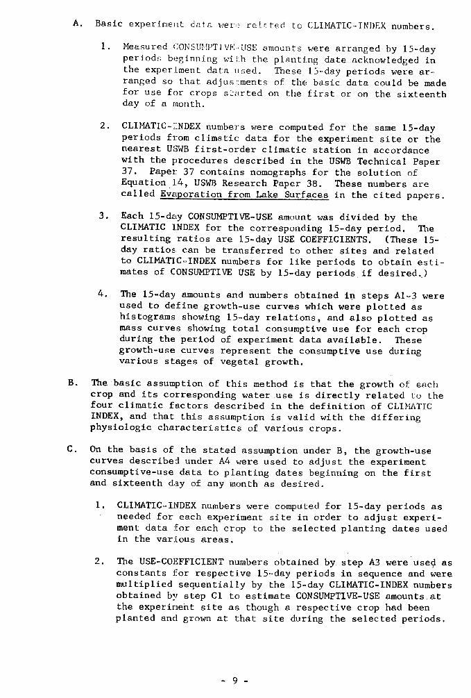
A. Basic experiment data ~,en:~ reL" ted to CLlMATIC·- INDEX numbers.

1. Measured CONSUlfPTlVE··· USE amounts were arranged by IS-dayperiods beginning with the planting date acknowledged inthe experiment data used. These IS-day periods were ar­ranged so that adjustments of the basic data could be madefor use for crops s~arted on the first or on the sixteenthday of a month.

2. CLIMATIC-INDEX numbers were computed for the same IS-dayperiods from climatic data for the experiment site or thenearest USWB first-order climatic station in accordancewith the procedures described in the USWB Technical Paper37. Paper 37 contains nomographs for the solution ofEquation.14, USWB Research Paper 38. These numbers arecalled Evaporation from Lake Surfaces in the cited papers.

3. Each IS-day CONSUMPTIVE-USE amount was divided by theCLIMATIC INDEX for the corresponding IS-day period. Theresulting ratios are IS-day USE COEFFICIENTS. (These IS­day ratios: can be transferred to other sites and relatedto CLIMATIC-INDEX numbers for like periods to obtain esti­mates of CONSUMPTIVE USE by IS-day periods if desired.)

4. The IS-day amounts and numbers obtained in steps Al-3wereused to define growth-use curves which were plotted ashistograms showing IS-day relations, and also plotted asmass curves showing total consumptive use for each cropduring the period of experiment data available. Thesegrowth-use curves represent the consumptive use duringvarious stages of vegetal growth.

B. The basic assumption of this method is that the growth of eachcrop and its corresponding water use is directly related to thefour climatic factors described in the definition of CLI~~TIC

INDEX, and that this assumption is valid with the differingphysiologic characteristics of various crops.

C. On the basis of the stated assumption under B, the growth-usecurves described under A4 were used to adjust the experimentconsumptive-use data to planting dates beginning on the firstand sixteenth day of any month as desired.

1. CLIMATIC-INDEX numbers were computed for IS-day periods asneeded for each experiment site in order to adjust experi­ment data for each crop to the selected planting dates usedin the various areas.

2. The USE-COl~FFICIENT numbers obtained by step A3 were usec;I asconstants for respective IS-day periods in sequence and weremultiplied sequentially by the IS-day CLIMATIC~INDEX numbersobtained by step Cl to estimate CONSUMPTIVE-USE amounts atthe experiment site as though a respective crop had beenplanted and grown at that site during the selected periods.

- 9 -

3. The CONSUMPTIVE-USE amounts and the CLIMATIC-INDEX numberscomputed by steps Cl and C2 were combined into desired half­month and full-month arrangements to agree with the desiredplanting dates and the adopted length of growing season.

4. The half-month and full month values as combined in step C3were then processed: UC/IC=KU--CONSUMPTIVE USE divided byCLIMATIC INDEX equal s USE COEFFICIENT.

The KU numbers computed by the above-described procedure comprised sets ofconstant-value USE COEFFICIENTS which were employed in the computation of esti­mates of CONSUMPTIVE-USE amounts for respective crops in the areas of majorproduction as desired.

BASIC DATA

Consumptive Use of Water by Crops

Amounts of water used consumptively by various crops~ as determined atbasic research and experiment sites~ and presented in published and unpublishedreports, were part of the basic data used to develop the relations and esti­mated consumptive-use amounts described and presented herein. These data wereobtained at various sites in Arizona~ Ca1ifornia~ and Texas. The sources ofdata for respective crops~ are as follows:

Alfalfa consumptive-use amounts in San Fernando Valley, Ca1ifornia~

in 1940 :2.1

Corn based on consumptive-use amounts for grain sorghum at Bushland,Texas~ 1956-58 2/,&/ and adjusted on the basis of growth-userelations for the two crops as indicated by figure 29 in Bulle­tin 937 1/

Cotton consumptive-use amounts at Weslaco, Texas, in 1958 §./

Small Grains consumptive use at Bush1and~ Texas~ 1956~58 2/ ,E/

2/ Blaney~ H. F.~ Haise, H. R., and Jensen, M. E., Monthly ConsumptiveUse by Irrigated Crops in Western Ul1Iited States: Supplement to U. S. SoilConservation Service Tech. Paper 96.

6/ Jensen, M. E., and Sletten~ W. H., 1959, Agricultural Reasearch ServiceProject Reports: ARS-SWC, Fort Col1.ins~ Colorado and Bushland~ Texas.

7/ Bloodworth, M. E., 1959, Some Principles and Practices in the Irriga­tion of Texas Soils: Texas Agricultural Experiment Station Bull. 937, A. & M.College of Texas.

8/ Ross, P. E., and Boykin, J. W., Unpublished data for 1958 cotton cropat ARS-SWG station in Weslaco, Texas.

- 10 -

Citrus consumptive use is average of amounts for oranges and grape­fruit in Salt River Valley, Arizona, 1931-54 ~/ and the amountsfor oranges in San Fernando Valley, California, in 1940 :2.1

Deciduous Fruit consumptive use in San Joaquin-Sacramento Delta,California, in 1928 2/

Pecans consumptive use based on amounts for walnuts in San FernandoValley ~ California, in 1928 :2./

Peanuts estimated average consumptive use in east Texas based ondata in Bulletin 937 1/

Rice consumptive use and cultural flooding based on data from Rice­Pasture Experiment Station at Beaumont and Eagle Lake, Texas,in 1954

Grain sorghum consumptive use at Bushland, Texas, 1956-58 1/,~/

Deep-Rooted Vegetables consumptive use by tomatoes in SacramentoValley, California, 1933-55 ~/

Shallow-Rooted Vegetables consumptive use in San Joaquin Delta,California, in 1928 1/

The relations of the consumptive use of water by perennial pasture; byleguminous or other crops, used as fertilizers or soil conditioners; by silagesorghum and forage sorghum; to the consumptive use by the base crops describedpreviously, were determined on the basis of sparse experiment data and recom­mendations by some of the agriculturists acknowledged.

The basic amounts of consumptive use at respective experiment sites by theabove crops, as used to develop the USE COEFFICIENTS employed in the TBWE Meth­od, are shown on table 1 (appendix B, page B-3). In some instances, the amountsshown as UC (CONSUMPTIVE USE) vary slightly from the amounts presented in thecited references. These variations result from the adjustment of the experi­ment data because of differences in planting dates.

1/ See footnote 5, page 10.

6/ See footnote 6, page 10.

1/ See footnote 7, page 10.

9/ Blaney, H. F., March 1959, Monthly Consumptive Use Requirements forIrrigated Crops: Am. Soc. Civil Engineers Proc. Paper 1963, Journal of theIrrigation and Drainage Division, Vol. 85, No. lR-l, Part I.

- 11 -

Climatic Index

The basic value of the average annual CLIMATIC INDEX determined for eachof the 24 areas of the state described under GENERAL DISCUSSION, Divisions ofthe State, is shown by the large numerals on figure 3 (appendix A, page A~5).

These values were obtained by replotting the respective isograms shown on plate2, USWB Technical Paper 37, onto a map of Texas showing the 24 areas, and thendetermining an average from these isograms in each area. The resulting chartshows the variation in the average-annual value of the CLIMATIC INDEX for thelO-year period 1946-55 across the State.

As mentioned before, the values shown on plate 2, USWB Technical Paper 37,and entitled:"AVERAGE ANNUAL LAKE EVAPORATION IN INCHES, PERIOD 1946-55", arecalled CLIMATIC~INDEX numbers in this report.

Monthly values of the CLIMATIC-INDEX numbers for each of the 24 areas weredetermined by multiplying the average annual CLIMATIC~INDEX number for an areaby the monthly distribution coefficients for that area as shown in table 3(appendix B9 page B-7). These distribution coefficients were determined fromvalues of the average monthly CLIMATIC~INDEXnumber computed for 31 USWB first­order climatic stations--20 in Texas and 11 in adjacent states. These first­order stations are listed in table 2: (appendix Bo page B-6). The distributioncoefficients are the ratios obtained by diViding the average monthly CLIMATIC­INDEX number by the average annual CLIMATIC~INDEX number 0 If expressed as apercentage 9 these coefficients repre,sent the percentage of the annual CLIMATIC­INDEX number occurring each month of a year on an average. The distributioncoefficients were assigned to each of the 24 areas on the basis of the defi­nition afforded by the numbers computed for each first-order climatic station-­using such numbers direct when applicable 9 and interpolating between suchnumbers for adjacent areas when applicable. The resulting CLIMATIC-INDEXnumbers are shown in table 3.

Monthly values of the CLlMATIC~INDEX number were computed for each experi~

ment site 9 for each year or each average of years, as needed for relating toCONSUMPTIVE-USE amounts for crops comprising the basic agricultural data usedherein. These numbers are shown as IC for the respective sites and crops intable L

USE COEFFICIENTS

Constant-value USE C.oEFFICIENTS for each crop at each experiment sitewere computed from the basic data as previously described under TBWE METHOD,Procedure of C0!!!E!!tation.. For practical application of the method~ the USECOEFFICIENTS for half-month periods were recomputed and related to one-halfof a monthly CLIMATIC-INDEX number. This procedure allows the use of monthlyvalues of the CLIMATIC~INDEX number divided by two when computing estimatesof consumptive use by crops planted on the sixteenth of a month or harvestedby the fifteenth of a month. The USE COEFFICIENTS for each crop and eachstarting date and length of growing season are shown as KU in table 1.

The consumptive-use amounts computed and shown for each crop are esti­mates of the average depth of water:1 in inches, reqUired for the growth andfull development of that crop under conditions favorable to the production of

- 12 -

eel .Iiral (:1"( ps hiclvn

r~ri()d; indicaud, Ihl'slelude i;3timates of 1 :s:;e

other causes not inbenmdescribed and uEed.

i fulI ;~.ater supply in ,each of the areas for theinlounts .are constituted as defined and do not in­l,f 'IJ.ater from distribution, leaching, seepage, andy a pH r I: 1)£ the experimen t cansump tive-use data

TABULATIONS OF DATA

A set of tables, numbers 1 to 4 (appendix B) and numbers 5 to 16 (appen­dix C), are used to present the rE~ la tions described and the resul ts obtainedby the procedures set forth. TheBe tables contain the basic experiment CON­SUMPTIVE-USE data adjusted to planting dates used herein, the CLIMATIC-INDEXnumbers for the experiment sites, the TBWE USE COEFFICIENTS evolved, the dis­tribution coefficients used to convert average-annual climatic-index numbersto monthly numbers in the 24 areas covering Texas, the average-monthly and ­average-annual climatic-index numbers computed for each of the 24 areas, andmonthly and seasonal consumptive-use amounts by areas for the crops includedand listed under GENERAL DISCUSSION, Crops and Crop Groupings.

The 24 areas were listed on the tables in a sequence chosen to attainreasonably smooth transi tion betwE~en the extremes in the general geographicand climatic areas of the State.

- 13 -

SELECTED BIBLIOGRAPHY

Abbe, Cleveland, 1905, A First Report ,6f the·Relations Between Climates and Crops:U. S. Weather Bureau Bull. 36.

Allen, S. W.O, 1955, Conserving Natural Resources, Principles and Practices in aDemocracy: New York, McGraw-Hill Book Company.

Am. Geophys. Union, June 193 t.,., Report of the Committee on Absorption and transpi­ration,1933-34: Am. Geophys. Union Trans., Washington, U. S. Govt. PrintingOffice.

Am. Soc. Civil Engineers, 1952, Consumptive Use of Water: Paper 2524 - a sympo­sium, Am. Soc.' Civil Engineers Trans., VoL 117.

_____________, 1930 li Corisumptive Use of Water in Irrigation: ProgressReport of the Duty of Water Committee of the Irrigation, Am. Soc. Civil Engi­neersTrans., Vol. 94.

___~_--:--: , 19q·9, Hydrology Handbook: Am. Soc. Civil EngineersManuels of Engineering Practice, No. 28.

Beauchamp, K. H., September 1958~ Potential Use of Water by Irrigation in theHumid Area: Am. Soc. Civil Engineers Proc. Paper 1750, Journal of the Irri­gation and Drainage Division, Vol. 84, No. lR-3.

Biggar, J. W., Bloodworth, M. E., and Burleson, C. A., 1957, Effect of IrrigationDifferentials and Planting Dates on the Growth, Yield, and Fiber Characteris­tics of Cotton in the Lower Rio Grande Valley: Texas Agricultural ExperimentStation Progress Report 1940, A. & M. College of Texas.

Blanney, H. F., 1952, Consumptive Use of Water: Am. Soc. Civil Engineers Trans.,Vol. 117.

______________ , October 1955, Evaporation and Evapotranspiration Investigationsin the San Francisco Bay An~a: Am. Geophys. Union Trans., Vol. 36, No.5.

_____________ , 1938, Field Methods of Determining Consumptive Use of Water:Division of Irrigation, U. S. Dept. of Agriculture.

_______, March 1959, Monthly Consumptive Use Requirements for IrrigatedCrops: Am. Soc. Civil Engineers Proc. Paper 1963, Journal of the Irrigationand Drainage Division, Vol. 85, No. lR~l, Part I.

________, and Criddle, ~1. D., August 1950, Determining Water Requirementsin Irrigated Areas from Climatological and Irrigation Data: U. S. Soil Con­servation Service Tech. Pape:r 96.

___________ , Ewing, P. A., Morin. K. V., and Criddle, W. D., June 1942, Con­sumptive Water Use and Requirements: Natl. Resources Planning Board, PecosRiver Joint Investigation - Reports of the participating agencies, Washington,U. S. Govt. Printing Office.

- 15 -

Blaney, H. F., Ewing, P, A., Israe1sen, 0, W., Rohwer, Carl, and Scobey, F. C.,

February 1938, Water Utilization, Upper Rio Grande Basin: National Resources

Committee, Part Ill.

_____________ , Haise, H. R., and Jensen, M. E., August 1950, Monthly Consumptive

Use by Irrigated Crops in Western l~ited States - a Provisional Supplement to

SCS-TP-96, Determining Water Requirements in Irrigated Areas from Climatolo­

gical and Irrigation Data: U. S. Soil Conservation Service Tech. Paper 96.

__________ , and Harris, Karl, December 1951, Consumptive Use and Irrigation

Requirements of Crops in Arizona: U. S. Soil Conservation Service.

__________~--, and Morin, K. V., 1942, Evaporation and Consumptive Use of Water

Empiricai Formulas: Am. Geophys. Union Trans., Vo 1. 23.

______________ , and Stockwell, H. J., Jr., June 1941, Progress Report on Cooper­

ative Research Studies on Water Utilization, San Fernando Valley, California,

Irrigation Season of 1940: Division of Irrigation, U. S. Dept. of Agriculture.

______________ , Taylor, C. A., Nickle, M. G., and Young, A. A., 1933, Water Losses

Under Natural Conditions from Wet Areas in Southern California: Division of

Water Resources Bull. 44, California State Dept. of Public Works, Pomona,

California.

______________ , Taylor, C~ A., and Young, A. A., 1930, Rainfall Penetration and

Consumptive Use of Water in Santa Ana River Valley and Coastal Plain: Division

of Water Resources Bull. 33, California State Dept. of Public Works, Pomona,

California,

Bloodgood, D. W., Lno dat~/, Biennial Reports: Texas Board of Water Engineers,

Austin, Texas.

and Curry, A. S., 1925, Net Requirements of Crops for Irri­

gation Water in the Mesilla Valley, New Mexico: New Mexico Experiment Station

Bull. 149.

Bloodworth, M. E., September 1959, Some Principles and Practices in the Irri­

gation of Texas Soils: Texas Agricultural Experiment Station Bull. 937,

A, & M. College of Texas.

____~------------, Burleson, C. A., and Cowley, W. R., 1956, Effect of Irrigation

Differentials and Planting Dates on the Growth, Yield, and Fiber Characteris­

tics of Cotton in the Lower Rio Grande Valley: Texas Agricultural Experiment

Station Progress Report 1866, A. ,s. M. College of Texas.

, Cowley, W. R., and Morris, J. S., 1950, Growth and Yield of

----------------Cotton on Willacy Loam as Affected by Different Irrigation Levels: Texas

Agricultural Experiment Station Progress Report 1217, A. & M. College of Texas.

Bodman, G. B., and Colman, E. A., 1944, Moisture and Energy Conditions During

Downward Entry of Water into Moist and Layered Soils: Am. Soil Science Society

Proc., Vol. 8.

Bonnen, C. A., McArthur, W. C., Magee, A. C., and Hughes, W. F., 1952, Use of

Irrigation Water on the High Plai.ns: Texas Agricultural Experiment Station

Bull. 756, A. & M. College of Texas.

- 16 -

Briggs, L. J., and Shantz, H. L.~ October 1916, Daily Transpiration During theNormal Growth Period and its Correlation with the Weather: Journal of Agri­cultural Research, Vol. 7.

______________ , and Shantz, H, L., January 1916, Hourly Transpiration Rate onClear Days as Determined by Cyclic Environmental Factors: Journal of Agri­cultural Research, Vol. 5,

Colman, E. A" and Bodman, G. B., 1945, Moisture and Energy Conditions DuringDownward Entry of Water into Moist and Layered Soils: Am. Soil Science SocietyProc., Vol. 9.

Conkling, H., 1930, Consumptive Use of Water in Irrigation: Progress Report ofthe Duty of Water Committee of the Irrigation 'Division, Am. Soc. Civil Engi­neers Trans., Vol. 94.

Criddle, W. D., January 1958, Influence of Climate on Irrigation Agriculture:Am. Soc. Civil Engineers Proc. Paper 1504, Journal of the Irrigation and brain­age Division, Vol. 84, No. lR-l.

_____________ , January 1958, Methods of Computing Consumptive Use of Water: Am.Soc. Civil Engineers Proc. Paper 1507, Journal of the Irrigation and DrainageDivision, Vol. 84, No. lR-l.

Davis, J., R., August 1956, Future of Irrigation in Humid Areas: Journal of theAm. Water Works Assoc., Vol. 48, No.8.

____________ , 1956, Water Demand Potential of Irrigation in Humid Areas: Reportto Indiana Water Resources Study Committee, Purdue University, Lafayette,Indiana.

Draper, E. L. July 1947, Supporting Data, Middle Rio Grande Project Report Studyof Valley Consumptive Use and Irrigation Demand at Otowi: U. S. Bureau ofReclamation, Albuquerque, New Mexico.

Fisher, C. E" and Burnett, E., 1953, Conservation and Utilization of SoilMoisture: Texas Agricultural Experiment Station Bull. 767, A. & M. Collegeof Texas.

Fortier, Samuel, 1927, Orchard Irrigations: U. S. Dept. of Agriculture Farmers'Bul L 1518.

____________ , and Young, A. A., June 1930, Irrigation Requirements of theArid and Semiarid Lands of the Southwest: Division of Agricultural Engi­neering Tech. Bull. 185, Bureau of Public Roads, U. S. Dept. of Agriculture,Washington, U. S. Govt. Printing Office,

Gardner, W., and Widtsoe, J" 1921, The Movement of Soil Moisture: Soil Science,11.

Garton, J. E. A" July 1951, Graphic Method of Finding the Depth of IrrigationApplied: Agricultural Engineering.

Gatewood, J. S., Robinson, T. H., Colby, B. R., Hem, J. D., and Halpenny, L. C.,1950, Use of Water by Bottom.. Land Vegetation'in Lower Safford Valley, Arizona:U. S. Geo1. Survey Water-Supply Paper 1103 .

.. 17 -

Gerard, C. J., Bloodworth, M. E., Burleson~ C. A.~ and Cowley, W. R., 1958,Cotton Irrigation in the Lower Rio Grande Valley: Texas Agricul tural Ex­periment Station Bull. 916, A. lit M. College of Texas.

_____________ , Burleson~ C. A. ~ Biggar~ J. Wo, and Cowley, W. R.~ 1958~ Effectof Irrigation Differentials and Planting Dates on Yield of Cotton in the LowerRio Grande Valley: Texas Agricultural Experiment Station Progress Report 2016,A. & M. College of Texas.

Halkias, N. A., Veihmeyer, F. J. ~ and Hendrickson, A. H., December 1955, Deter­mining Water Needs for Crops from Climatic Data: Hilgardia~ Vol. 24, No.9,University of California.

Hall, W. A" April 1956~ Estimating Irrigation Border Flow: Agricultural Engi­neering.

Hansen, V. E., February 2~ 1955~ Infiltration and Soil Water Movement DuringIrrigation: Soil Science, 79.

Hargreaves, G. H., November 1956, Irrigation Requirements Based on Climatic Data:Am. Soc. Civil Engineers Proc. Paper 1105~ Journal of the Irrigation and Drain­age Division, Vol. 82, No. lR-3.

Harris, Karl, Kinnison, A. F.~ and Albertt, O. W.~ 1936, Use of Water by Wash­inton Navel Oranges and Marsh Grapefruit Trees in Salt River Valley, Arizona:Arizona Agricultural Experiment Station Bull. 153.

Hildreth, R. J., 1956, Risk and Uncertainty Arising From Soil-Moisture YieldRelationships in the Great Plains: Paper for Southwestern Social ScienceAssociation Program, March 30, 1956, Dept. of Agricultural Economics andSociology, A. & M. College of Texas.

Horton~ R. E., 1923, Transpiration by Forest Trees: U. S. Weather Bureau MonthlyWeather Review~ Vol. 51.

Hughes, W. F., and Motheral~ J. R., September 1950, Irrigated Agriculture inTexas: Texas Agricultural Experiment Station Misc. Pub. 59, A. & M. Collegeof Texas.

Iowa State University, July 1959, Chances of Receiving Selected Amounts of Pre­cipitation in the North Central Region of the U. S.: Iowa Agricultural andHome Economics Experiment Station, Ames, Iowa.

______________________ , Lno dat~/, Transpiration and Evapotranspiration as Re­lated to Meteorological Factors (U. S. Weather Bureau Contract 9295): IowaAgricultural and Home Economics Experiment Station, Ames, Iowa.

Israelsen~ O. W., September 1958, The Engineer and Worldwide Conservation ofSoil and Water: Am. Soc. Civil Engineers Proc. Paper 1775, Journal of theIrrigation and Drainage Division, Vol. 84~ No. lR-3.

, 1950, Irrigation Principles and Practices: New York, John---------~-----Wiley and Sons, Inc.

Jensen, M. E., 1957, Research Shows \fuen to Irrigate Winter Wheat: Soils andWater.

- 18 -

Kansas StatE! ColJ.egl~, 1956-57, The Evapotranspiration Problem First ContributionRepcrt (U. S. Heather Bureau Contract 8806): Manhattan, Kansas.

Kohler, K. 0.:. Jr., 1955, Trends in the Utilization of Water: Yearbook of Agri­culture.

Kohler, M. A' it 1957 ~ Computat:Lon of Evaporation ~nd Evapotranspiration from Me­teorologic:al Observations: Paper for presentation at Am. Meteorological Soci­ety Meeting in Chicago, Mareh 19~2l, 1957.

, Nordenson, T. J., and Baker, D. R., 1959, Evaporation Maps for theUnited States: U. S. Weather Bureau Tech. Paper 37.

__---------------, Nordenson, T. ,T., and Fox, W. E., 1955, Evaporation from Pans andLakes: U. S. Weather Bureau Research Paper 38.

Linsley, R. K., Lno dat~/, Techniques for Surveying Surface-Water Resources:World Meteorological Organi:i~ation No. 82, Tech. Paper 32, Tech. Note 26.

Lowry, R. L., Jr., and Johnson, A. F., April 1941, Consumptive Use of Water forIrrigation: Am. Soc. Civil Engineers Proc., Vol. 67.

___________, and Johnson, A. F., 1942, Consumptive Use of Water for Agri­culture: Am. Soc. Civil Engineers Trans., Vol. 107.

McCulloch, A. A., August 1957, The Economics of Sprinkler Irrigation Systems:Irrigation - Engineering and Maintenance.

Magee, Ao C., Bonnen, C. A., ~~Arthur, W. C., and Hughes, W. F., 1953, ProductionPractices for Irrigated Crops on the High Plains: Texas Agricultural Experi­ment Station Bull. 763, A. 0: M. College of Texas.

Maierhofer, C. R., January 1958, Drainage in Relation to a Permanent IrrigationAgriculture: Am. Soc. Civil Engineers Proc. Paper 1506, Journal of the Irri­gation and Drainage Division, Vol. 84, No o lR-l.

Mickey, K. B., 1945, Man and The Soil: International Harvester Company.

Muldrow, W. C., 1948, Forecasting Productivity of Irrigable Lands: Am. Soc. CivilEngineers Trans., Vol. 113.

Nettles, V. F., Jamison, F. S;, and Jones, B. E., June 1952, Irrigation and OtherCultural Studies with Cabbage, Sweet Corn, Snap Beans, Onions, Tomatoes andCucumbers: University of Florida Agricultural Experiment S~ation Bull. 495,Gainsville, Florida.

Osborn, Ben, Lno dat~/, Water and the Land: Uo S. Soil Conservation ServiceTech. Paper 134.

Palmer, V. .I., April 1946, Retardance Coefficients for Low Flow in ChannelsLines with Vegetation: Am. Geophys. Union Trans. 27.

Palmer, W. C., April 1958, A Graphical Technique for Determining Evapotrans­piration by the Thornwaite Method: U. So Weather Bureau, Washington, U. S.Govt. Printing Office.

- 19 -

Parshall, R. L., 1937, Laboratory Measurement of Evapo-Transpiration Losses:Journal of Forestry, pp. 1033-1040.

Penman, H. L., February 1956, Estimating Evaporation: Am. Geophys. Union Trans.,Vol. 37, No. 1.

____--:"'__, 1948, Natural Evaporation from Open Water, Bare Soil and Grass:Proceedings of the Royal Society, Series A-193, London, England.

_____________ , 1952, Water and Plant Growth: Agricultural Progress, Vol. 27,Part 2.

Pruitt, W. 0., and Jensen, M. C." June 1955, Determining when to Irrigate:Agricultural Engineering.

Ree, W. 0., 1939, Some Experiments on Shallow Flows Over a Grassed Slope: Am.Geophys. Union Trans., Part IV"

Reynolds, E. B., 1954, Research on Rice Production in Texas: Texas AgriculturalExperiment Station Bull. 775, A. & M. College of Texas.

Robinson, A. R., Jr., and Rohwer, Carl, 1957, Measurement of Canal Seepage: Am.Soc. Civil Engineers Trans., Vol. 122.

Russell, E. J q 1950, Soil Conditions and Plant Growth: New York, Longmans,Green and Company.

Shaw, B. T. (Editor), 1952, Soil Physical Conditions and Plant Growth: New York,Academic Press.

South Dakota State College, February 1959, Seasonal Variations of Soil Moisturein South Dakota: South Dakota Agricultural Experiment Station, EconomicsDept. Pamphlet 99, Brookings, South Dakota.

Staten, T. D., 1957, Alfalfa Production in Texas: Texas Agricultural Experi­ment Station Bull. 955, A. & M. College of Texas.

Swanson, N. P., and Thaxton, E. L., 1956, Irrigation ReqUirements for GrainSorghum Production on the High Plains: Texas Agricultural Experiment StationBull. 846, A. & M. College of Texas.

Texas Agricultural Experiment Station, June 1954, Summary of Soil and Water Con­servation Research from the Blackland Experiment Station, Temple, Texas, 1942~

53: Texas Agricul tural Experiment Station Bull. 781, A. & M. College of Texas.

Texas Crop and Livestock Reporting Service, Ino date/, Texas Vegetable Statis­tics, 1939-58: Agricultural Marketing Ser;ice, U~ S. Dept. of Agriculture.

Thaxton, E. L., and Swanson, N. Po, 1956, Guides in Cotton Irrigation on theHigh Plains: Texas Agricultural Experiment Station Bull. 838, A. & Mo Collegeof Texas.

Thornthwaite, C. We' 1948, An Approach toward a Rational Classification of Cli­mate: Geographical Review 38.

- 20 -

Thornthwaite l , C. 1-1", and Mather~ J. R., 1957, Instructions and Tables for Com­puting Potemtial Evapotranspiration and the Water Balance: Drexel Instituteof Technology Pub. in Climatology, Vol. X, No" 3, Centerton, New Jersey.

___________ , and Mather, J. R., 1955, The Water Ba lance: Drexel ins ti­tute of Technology Pub. in Climatology, Vol. VIII, No.1, Centerton, New Jersey.

Thornton, J. D., and Templin, E. H., Lno dat~/, The Soils of Texas: Texas Agri­cultural Extension Service Leaflet 74, A. & M. College of Texas.

Thurmond, R. V., /~o dat~/, How to Estimate Soil Moisture by Feel: Texas Agri­cultural Extension Service Leaflet 355, A. & M. College of Texas.

_________, Lno dat~/t Soil Moisture Storage: Texas Agricultural ExtensionService Leaflet 357, A. & M. College of Texas.

Cotton:Texas.

Trew, E. M., and Hoveland, C. S., 1955, Irrigated Pastures for South Texas: Tex­as Agricultural Extension Service and Texas Agricultural Experiment StationBull. 819, A. & M. College of Texas.

U. S. Geological Survey, 1954, Water-Loss Investigations: Vol. 1 - Lake HefnerStudies: U. S. Geol. Survey Prof. Paper 269.

_____________________, 1958, Water-Loss Investigations: Lake Mead Studies:U. S. Geol. Survey Prof. Paper 298.

Van Bavel, C. H. M., 1953, A Drought Criterion and Its Application in EvaluatingDrought Incidence and Hazard: Agronomy Journal, Vol. 45.

_____________ '. and Wilson, T. V., 1952, Evapotranspiration Estimates asCriteria for Determining Time of Irrigation: Agricultural Engineering, Vol. 33.

Veihmeyer, F. J., 1938, Evaporation from Soils and Transpiration: Am. Geophys.Union Trans., Vol. 19.

Young, A. A., 1945, Irrigation Requirements of California Crops: Division ofWater Resources Bull. 51, California State Dept. of Public Works, Pomona,California.

___________ , and Blaney, H. F., 1942, Use of Water by Native Vegetation: Cali­fornia State Division of ~rater Resources Bull. 50, Sacramento, California.

- 21 -

APPENDIX A

Descriptive Figures

A-I

EXPLANATION

I H10h Plolns

2 Trans - Pecos

3 Edwards Plaleau - Central Basin

4 Rio Grande Plain

!l Coastal Prairie

6 Eost Tuas Tlmborland.

1 Blackland - Grand Prairies

8 North Central Pralrl .. _0 Roilino Plains

Balld on map. In MI!lcellaneoue Publication 59 and Bulletin 937, Texas

Aoricuiturai Elperlment Station, A. 8 M. Coll,q, of Tlll.os.

October 1960

FIGURE I.

o &0 '00 Mu..

....Cl.l£:lwlli==::I1

Land resource divisions and Irrigated areas.

A-3

Te~Boord of Water Engineers

N

IAr o

--

I- __ -_.It'

IBIII

8B I

------ r'I

IeII

October 1960

FIGURE 2. - Subdivisions of irrigated areas

A-4

Bulletin 6019

Tell.o! Boord of Water Engineers Buitetln l;i019

EXPLANATION

1A Subdivisions of Irrigated (Ireos (fig, 2)

'-- 64-lsooram9 of CUMATIC - INDEX numbers V ,T

Average~(Jnnu(]1 value of CLIMATIC INDEX

for each Indicated subdivision (table 3)65

II Average-annual numbers, for the period 1946-55, as expressed on plate 2 ofthe U. S. Weather Bureau Technical Paper No. 37\ Evaporation Maps for theUnited States.

Oetober 1960

FIGURE 3.- Average-annual CLIMATIC-INDEX numbers for subdivisions

of irrigated areas

A-S

Texas Board ot Waler EngineersBullelin 6019

Area Jan. Feb. Mar. Apr. Hay June July Aug. Sept. Oct. Nov. Dec. Area Jan. Feb. Mar. Apr. May June July Aug. Sept. Oct. Nov. Dec.

i---i

----........---~

~1-r~~~I------:--~

Ir·--- - -------.- --------,

I

I - i- ,- ~.

! ii

GRAINS. SMALL

ORCHARDS, CITRUS

4A

4C H: I I iii I ,i!48 [ I ! : I ==4A: I . Iii

ORCHARDS, DECIDUOUS FRUIT

ORCHARDS. PECAN

5A I D RICE

~~~ i II i:

Ell §d I II i I :n3B

I7AI7B

6A ,6BI

!6C

iI

7C

1~~~f Id I I I I I ! J8B - I \ I;~ I I: !2C ' 1'-'- ....'---....

3A I I3BSA7A7B6A686C7C5A5B5C4D4E4C4B

CORN

§b!d#1i I I ~ II I : .

! ! ! t I

i II ~I ! i I II _I I I\ - \ i i

iA I I· 00""

~! I I I I·: 1 I II ! I Il- , I j I I

lAlBlC8B2A2B2C3A3B8A7A7B6A6B6C7C5A5B5C4D4E4C4B4A

~~ I 'i !~ ~ I' I: ISA ! i _.--+-i-+.~...J.... .....J7A ' I, I

Ii i Ii! i I ! r-40 I i I I I4E I I

4C4B I I I

4AI

>B

Q'\

FIGURE 4.-Average planting date and length of growing season of crops. by areas. in Texas

rexas Board of Water Engineers Bulletin 6019

Area Jan. Feb. Mar. Apr. May June .July Allg. Sept,- Oct. Nuv. D.,,::. Area Jan. Feb. Mar. Apr. May June July Aug. Sept. Oct. Nov. Dec.

1

I .

I I: !I

VEGETABLES, SHALLOW-RQ01'EDI ! I: -I

I II

I

I~ II

l:I I

VEGETABLES. DEEP-ROOTED

4A

IB2A8A7A786A686C7C5C404E4C48

~28 ! EJ I I Ii2C8A7A78

I

6A6B6C I

7CI

40 I4C

I

4BI I 1-

4A I i=

SORGHUM GRAINLA18IC8B2A282C

IJA388A7A786A6B6C

I7C5A58

I

5C404E4C484A

3B I~EA"UTS

786A6B6C7C40

:x:­I

--..J

Note.--Alfalfa, a perennial usually planted in September, is omitted from the above chart. The average planting date used for each crop is the first or middle;r-; month as indicated. In some areas for some crops, two bars indicate two crops yearly.

FIGURE 4. -Continued

APPENDIX B

Tables of EKperiment Data and Basic Relations

B-1

Table 1

BASIC DATA

UC--CONSUMPTIVE USE; IC--CLlNATIC INDEX; KU--USE COEFFICIENT; values at experiment sites and times

Data Jan. Feb. Mar. Apr. May June July Aug. Sept. Oct. Nov. Dec. Season

UCICKU

1.32.2

0.59

1.62.7

0.59

3.13.8

0.82

ALFALFA:3.34.3

0.77

San Fernando Valley, California,6.7 5.4 7.8 4.25.9 5.4 7.6 5.9

1.14 1.00 1.03 0.71

19405.65.4

1.04

4.44.3

1.02

3.13.8

0.82

1.32.7

0.48

47.854.00.89

CdI

W

UCICKU

UCICKU

CORN: Based on grain sorghum at Bushland,Texas, 1956-58, planted on1.3 4.0 6.5 8.48.4 8.8 8.0 6.2

0.15 0.45 0.81 1.35

CORN: Based on grain sorghum at Bushland, Texas, 1956-58, planted on*0.4 2.8 4.6 7.3

8.4+2 8.8 8.0 6.20.09 0.32 0.58 1.18

1st day of a month*2.9

5.7+21.00

16th day of month6.75.7

1.18

23.134.20.68

21.632.90.66

UCICKU

COTTON: Weslaco,0.73.1

0.23

Texas,1.25.1

0.24

1958, planted on6.1 5.55.9 6.6

1.03 0.83

1st day of a month,4.5 *.047.4 7.8+2

0.61 0.10

5~-month season18.4~:-; ".:JL.u

0.58

UCICKU

COTTON: Weslaco,*0.3

3.1+20.18

Texas,1.35.1

0.25

1958, planted on4.0 7.25.9 6.6

0.68 1.09

16th day5.17.4

0.69

of a1.77.8

0.22

month, 5~-month season19.634.30.57

UCICKU

COTTON: Weslaco,*0.3

3.1+20.18

Texas,1.35.1

0.25

1958, planted on3.6 6.05.9 6.6

0.61 0.91

16th day6.47.4

0.86

of a month, 6~-month

5.5 3.57.8 4.5

0.71 0.77

season26.6., ,c.' ~

* One-half month.

Table i--Continued

BASIC DATA

Data Jan. Feb. Mar. Apr. Hay June July Aug. Sept. Oct. Nov. Dec. Season

GRAINS, SMALL: Bushland, Texas, 1956-58~ planted on 1st day of a month, 8-month season1.6 2.4 5.4 7.5 6.4 1.6 1.6 1.5 28.02.0 2.3 3.6 5.1 6.9 5.7 2.8 2.5 30.9

0.80 1.04 1.50 1.47 0.93 0.28 0.57 0.60 0.91

GRAINS, S~~L: Bushland, Texas, 1956-58, planted on 16th day of a month, 9-month season1.0 1.8 3.9 6.5 7.0 *3.1 *0.7 1.6 1.4 1.1 28.12.0 2.3 3.6 5.1 6.9 8.4+2 6.2+2 5.7 2.8 2.5 38.2

0.50 0.78 1.08 1.27 1.01 0.74 0.23 0.28 0.50 0.44 0.74

ORCHARDS, CITRUS: Average for oranges and grapefruit, Salt River Valley, Arizona, 1931-541.6 1.7 2.5 3.2 4.2 4.9 5.6 5.6 4.8 3.5 2.4 1.7 41.72.3 3.3 5.0 7.1 8.9 9.9 9.2 8.1 5.2 5.0 3.0 2.2 69.2

0.69 0.52 0.50 0.45 0.47 0.49 0.61 0.69 0.92 0.70 0.80 0.77 0.60

Oranges, San Fernando Valley, California, 19401.1 2.2 2.3 4.0 4.4 4.6 4.0 3.4 2.8 2.6 2.0 1.6 35.02.2 2.7 3.8 4.3 5.9 5.4 7.6 5.9 5.4 4.3 3.8 2.7 54.0

0.50 0.81 0.61 0.93 0.75 0.85 0.53 0.58 0.52 0.60 0.53 0.59 0.65

ORCHARDS, CITRUS: Average values0.60 0.66 0.56 0.69 0.61 0.67 0.57 0.64 0.72 0.65 0.66 0.68 0~62

California,2.8 0.86.2 3.4

0.45 0.24

UCICKU

UCICKU

UCIC

ttl KUI

.J:'

UCICKU

KU

UCICKU

ORCHARDS, DECIDUOUS FRUIT: San Joaquin-Sacramento Delta,1.0 2.2 3.8 6.0 6.8 4.82.4 4.8 4.3 5.8 7.2 6.7

0.42 0.46 0.88 1.03 0.92 0.72

192828.240.80.69

2.03.6

0.56

UCICKU

ORCHARDS, PECAN: San1.5 3.8 5.02.6 5.1 4.6

0.58 0.75 1.09

Fernando5.96.1

0.97

Valley,6.17.6

0.80

California, 19285.0 2.87.1 6.6

0.70 0.42

32.643.30.75

* One-half month.

Table l--Continued

BASIC DATA

Data Jan. Feb. Mar. Apr. May June July Aug. Sept. Oct. Nov. Dec. Season

PEANUTS: Estimated UC, East Texas, planted on 1st day of a month, 4-month season

DC 2.1 5.1 6.4 4.3 17.9

IC 5.6 6.6 7.1 6.6 25.9

KU 0.38 0.77 0.90 0.65 0.69

PEANUTS: Estimated UC, East Texas, planted on 1st day of a month. 5-month season

UC l.1 2.9 4.3 6.3 3.5 18.1

IC 5.6 6.6 7.1 6.6 5.1 3l.0

KU 0.20 0.44 0.61 0.95 0.69 0.58

PEANUTS: Estimated UC. East Texas, planted on 16th day of a month, 5-month season

DC *0.4 2.0 3.4 5.5 5.3 *l.3 17.9

IC 4.6+2 5.6 6.6 7.1 6.6 5.1+2 30.8

KU 0.15 0.33 0.49 0.80 0.90 0.54 0.58

IJ:lI

VI RICE: Based on data from Rice-Pasture Experiment Stations, Beaumont and Eagle Lake, Texas, 1954

UC 7.6 6.8 15.0 10.2 6.8 9.6 56.0

IC 4.2 6.8 7.5 6.8 6.8 6.0 38.1

KU l.80 l.00 2.00 l.50 1.00 1.60 1.47

SORGHUM, GRAIN: Bushland, Texas, 1956-58. planted on 1st day of a month

UC 3.6 7.4 8.1 3.7 2.2.3

IC 8.4 8.8 8.0 6.2., 1 I,J J.. • ....,.

KU 0.43 0.84 1.01 0.60 0.73

SORGHUM. G~IN: Bushland. Texas, 1956-58. planted on 16th day of a month

UC *0.9 5.8 8.6 5.0 *1.1 '::'1..:.:

Ie 8.4+2 8.8 8.0 6.2 5.7+2 30.0

KU 0.21 0.66 l.08 0.81 0.38 0.72

VEGETABLES,DCIeKU

DEEP-ROOTED: Tomatoes, Sacramento Valley,3.07.8

0.38

California, 1933-55,4.2 7.0 5.18.7 7.5 6.5

0.48 0.93 0.78

planted2.13.7

0.57

on 1st day at a manu!~. /

L1.,"+--, f. ,~,

)4 ... L

0.63

* One-half month.

Table l--Continued

BASIC DATA

Data Jan. Feb. Mar. Apr. May June July Aug. Sept. Oct. Nov. Dec. Season

VEGETABLES,UCICKU

DEEP-ROOTED: Tomatoes, Sacramento*1.2

6.1+20.38

Valley,3.37.8

0.42

California, 1933-55, planted on5.7 7.3 4.5 *0.88.7 7.5 6.5 3.7+2

0.66 0.97 0.69 0.43

16th day of a month22.835.40.66

tp!0\

VEGETABLES, SHALLOW-ROOTED: San Joaquin Delta, California, 1928, planted on 1st day of a monthUC 1.2 3.0 6.0 5.4 5.4 3.6 1.8 26.4IC 4.8 ,4.3 5.8 7.2 6.7 6.2 3.4 38.4KU 0.25 0.70 1.03 0.75 0.81 0.58 0.53 0.69

*One-half month.

Table 2

U. S. WEATHER BUREAU First-Order Stations

Texas

Abilene Dallas Houston San AngeloAmarillo Del Rio Laredo San AntonioAustin El Paso Lubbock VictoriaBrownsville Fort Worth Palestine WacoCorpus Christi Galveston Port Arthur Wichita Falls

Arkansas Louisiana New Mexico Oklahoma

Fort Smith Baton Rouge Albuquerque Oklahoma CityLittle Rock Lake Charles Clayton Th.lsaTexarkana Shreveport Roswell

Table 3

CLIMATIC-INDEX COEFFICIENTS

Coefficients for monthly distribution of average-annual,climatic-index numbers, by areas, 1946-55

Area Jan. Feb. Mar. Apr. May June July Aug. Sept. Oct. Nov. Dec. Year

1A 0.03 0.04 0.07 0.10 0.11 0.14 0.13 0.12 0.10 0.07 0.05 0.04 ' ,..,,..,.L.vv

1B .03 .05 .08 .10 .11 .14 .13 .13 .09 .07 .04 .03 ' ,-,,,l..vv

lC .03 .04 .07 .10 .12 .13 .14 .12 .10 .07 .05 .03 1.008B .03 .04 .07 .09 .11 .14 .14 .13 .10 .07 .05 .03 1.00

2A .03 .04 .07 .10 .D .14 .13 .li .10 .07 .05 .03 l.002B .03 .04 .07 .10 .12 .13 .14 .12 .10 .07 .05 .03 1.002C .03 .04 .07 .10 .12 .13 .14 .12 .10 .07 .05 .03 l.003A .03 -.04 .07 .09 .12 .13 .14 .12 .10 .08 .05 .03 1.00

to 3B .04 .04 .07 .09 .11 .13 .13 .12 .10 .08 .05 .04 1.00I

8A .03 .04 .07 .09 .11 .14 .14 .13 .10 .08 .04 .03 1.00-..J

7A .03 .04 .07 .09 .11 .14 .14 .14 .10 .07 .04 .03 1.007B •03 .04 .07 .09 .11 .13 .14 .14 .10 . .08 .04 .03 LOU

6A .03 .04 .07 .09 '.11 .13 .14 .13 .10 .08 .04 .04 1.006B .03 .04 .07 .09 .11 .13 .14 .14 .10 .07 .04 .04 LOa6C .03 .04 .07 .09 .11 .13 .14 .13 .10 .08 _.04 .04 l.007e .03 .04 .07 .09 .11 .13 .13 .13 .10 .08 .05 .:04 1.00

SA- .03 .05 .07 .09 .12 .13 .12 .12 .10 .08 .05 .04 l.005B .03 .04 .06 .09 .11 .14 .13 .13 .10 .08 .05 .04 l.005C .03 .04 .07 .09 .11 .13 .13 .13 .10 .08 .05 .04 l.004D .04 .05 .07 .08 .ll .12 .14 .13 .09 .08 .05 .04 l.00

4E .04 .05 .07 .09 .ll .12 .13 .13 .09 .08 .05 .04 l.004C .04 .05 .07 .09 .10 .12 .14 .13 .09 .08 .05 .04 l.004B .04 .05 .06 .09 .11 .12 .14 .13 .09 .08 .05 .04 l.004A .04 .05 .07 .09 .11 .12 .14 .12 .09 .08 .05 .04 l.00

Table 4

CUMATIC- INDEX. NUMBE RS

Average monthly and annual climatic-index numbers. by areas. 1946-55Area Jan. Feb. Mar. Apr. May June July Aug. Sept. Oct. Nov. Dec. Year

lA 2.0 2.6 4.6 6.5 7.2 9.1 8.4 7.8 6.5 4.6 3.2 2.6 65lB 2.1 3.5 5.6 7.0 7.7 9.8 9.1 9.1 6.3 4.9 2.8 2.1 70lC 2.2 2.9 5.1 7.3 8.8 9.5 10.2 8.8 7.3 5.1 3.6 2.2 738B 2.0 2.7 4.8 6.1 7.5 9.5 9.5 8.8 6.8 4.8 3.4 2.0 682A 2.2 2.9 5.1 7.3 9.5 10.2 9.5 8.0 7.3 5.1 3.6 2.2 732B 2.2 2.9 5.0 7.2 8.6 9.4 10.1 8.6 7.2 5.0 3.6 2.2 722C 2.2 3.0 5.2 7.4 8.9 9.6 10.4 8.9 7.4 5.2 3.7 2.2 74.., A

2.2 3.0 5.2 6.7 8.9 9.6 10.4 8.9 7.4 5.9 3.7 2.2 74In

ttl 3B 2.6 2.6 4.6 5.9 7.3 8.6 8.6 7.9 6.6 5.3 3.3 2.6 66I8A 1.9 2.6 4.5 5.8 7.0 9.0 9.0 8.3 6.4 5.1 2.6 1.9 64

co7A 1.6 2.2 3.8 5.0 6.0 7.7 7.7 7.7 5.5 3.8 2.2 1.6 557B 1..7 2.3 4.0 5.1 6.3 7.4 8.0 8.0 5.7 4.6 2.3 1.7 576A 1.5 2.0 3.6 4.6 5.6 6.6 7.1 6.6 5.1 4.1 2.0 2.0 516B 1.6 2.1 3.7 4.8 5.8 6.9 7.4 7.4 5.3 3.7 2.1 2.1 536C 1.6 2.2 3.8 4.9 5.9 7.0 7.6 '7.0 5.4 4.3 2.2 2.2 547C 1.6 2.2 3.8 5.0 6.0 7.2 7.2 7.2 5.5 4.4 2.8 2.2 555A 1.6 2.6 3.6 4.7 6.2 6.8 6.2 6.2 5.2 4.2 2.6 2.1 525B 1.6 2.2 3.2 4.9 5.9 7.6 7.0 7.0 5.4 4.3 2.7 2.2 545C 1.6 2.2 3.8 5.0 6.0 7.2 7.2 7.2 5.5 4.4 2.8 2.2 554D 2.6 3.3 4.6 5.3 7.3 7.9 9.2 8.6 5.9 5.3 3.3 2.6 664E 2.2 2.8 3.9 5.0 6.2 6.7 7.3 7.3 5.0 4.5 2.8 2.2 564C 2.4 3.0 4.2 5.4 6.0 7.2 8.4 7.8 5.4 4.8 3.0 2.4 6048 3.0 3.8 4.5 6.8 8.2 9.0 10.5 9.8 6.8 6.0 3.8 3.0 754A 2.4 3.0 4.2 5.4 6.6 7.2 8.4 7.2 5.4 4.8 3.0 2.4 60

APPENDIX C

Tables of Crop Consumptive Use

Average monthly and annual consumptive use,

depth in inches, by areas, 1946-55

C-l

Table 5

ALFALFA

Average monthly and annual consumptive use. depth in inches. by areas. 1946-55

Area Jan. Feb. Mar. Apr. May June July Aug. Sept. Oct. Nov. Dec. Year

lA 1.2 1.5 3.8 5.0 8.2 9.1 8.7 5.5 6.8 4.7 2.6 1.2 58.3IB 1.2 2.1 4.6 5.4 8.8 9.8 9.4 6.5 6.6 5.0 2.3 1.0 62.7lC 1.3 1.7 4.2 5.& 10.0 9.5 10.5 6.2 7.6 5.2 3.0 1.1 65.988 1.2 1.6 3.9 4.7 8.6 9.5 9.8 6.2 7.1 4.9 2.8 1.0 61.3

2A 1.3 1.7 4.2 5.6 10.8 10.2 9.8 5.7 7.6 5.2 3.0 1.1 66.22B 1.3 1.7 4.1 5.5 9.8 9.4 10.4 6.1 7.5 5.1 3.0 1.1 65.02C 1.3 1.8 4.3 5.7 10.1 9.6 10.7 6.3 7.7 5.3 3.0 1.1 66.93A 1.3 1.8 4.3 5.2 . 10.1 9.6 10.7 6.3 7.7 6.0 3.0 1.1 c. '7 t

v / • J..

n 3B 1.5 1.5 3.8 4.5 8.3 8.6 8.9 5.6 6.9 5.4 2.7 1.2 58.9t

4.5Vol 8A 1.1 1.5 3.7 8.0 9.0 9.3 5.9 6.7 5.2 2.1 .9 57.97A .9 1.3 3.1 3.8 6.8 7.7 7.9 5.5 5.7 3.9 1.8 .8 49.278 1.0 1.4 3.3 3.9 7.2 7.4 8.2 5.7 5.9 4.7 1.9 .8 51.4

6A .9 1.2 3.0 3.5 6.4 6.6 7.3 4.7 5.3 4.2 1.6 1.0 45.76B .9 1.2 3.0 3.7 6.6 6.9 7.6 5.3 5.5 3.8 1.7 1.0 47.26C .9 1.3 3.1 3.8 6.7 7.0 7.8 5.0 5.6 4.4 1.8 1.1 48.57C .9 1.3 3.1 3.8 6.8 7.2 7.4 5.1 5.7 4.5 2.3 1.1 49.2

5A .9 1.5 3.0 3.6 7.1 6.8 6.4 4.4 5.4 4.3 2.1 l.0 46.558 .9 1.3 2.6 3.8 6.7 7.6 7.2 5.0 5.6 4.4 2.2 1.1 48.45C .9 1.3 3.1 3.8 6.8 7.2 7.4 5.1 5.7 4.5 2.3 1.1 49.24D 1.5 1.9 3.8 4.1 8.3 7.9 9.5 6.1 6.1 5.4 2.7 1.2 58.5

4E 1.3 1.7 3.2 3.8 7.1 6.7 7.5 5.2 5.2 4.6 2.3 1.1 49.74C 1.4 1.8 3.4 4.2 6.8 7.2 8.7 5.5 5.6 4.9 2.5 1.2 53.24B 1.8 2.2 3.7 5.2 9.3 9.0 10.8 7.0 7.1 6.1 3.1 1.4 66.74A 1.4 1.8 3.4 4.2 7.5 7.2 8.7 5.1 5.6 4.9 2.5 1.2 53.5

Note.--PERENNIAL PASTURE: Use 90 percent of monthly amount shown for ALFALFA as estimate of consumptive use.

Table 6

CORN

Average monthly and annual consumptive use, depth in inches, by areas, 1946-55

Area Jan. Feb. Mar. Apr. May June July Aug. Sept. Oct. Nov. Dec. Year

LA *0.3 2.3 5.3 9.9 9.2 27.01B *.3 2.5 5.7 10.7 10.7 29.91e *.3 2.8 5.5 12.0 10.4 31.08B *.3 2.4 5.5 11.2 10.4 29.8

2A 1.1 4.3 8.3 12.8 *4.0 30.52B 1.1 3.9 7.6 13.6 *4.3 30.52C 1.1 4.0 7.8 14.0 *4.4 31.3.... 1.0 4.0 7.8 14.0 *4.4 31.2..;Jon.

n 3B .9 3.3 7.0 11.6 *4.0 26.8f

.9 3.2 7.3 12.2 *4.2 27.8.j:'- 8A7A .8 2.7 6.2 10.4 *3.8 23.97B *0.2 1.6 3.7 8.7 9.4 23.6

6A *.2 1.5 3.2 7.8 8.4 21.16B *.2 1.5 3.4 8.1 8.7 21.96C *.2 1.6 3.4 8.3 9.0 22.57C *.2 1.6 3.5 8.5 8.5 22.3

5A *.2 1.5 3.6 8.0 7.3 20.65B *.1 1.6 3.4 9.0 8.3 22.45C .6 2.2 4.9 9.7 *3.6 21.04D .7 2.4 5.9 10.7 *4.6 24.3

4E .6 2.2 5.0 9.0 *3.6 ~20.4

4C .6 2.4 4.9 9.7 *4.2 21.84B .7 3.1 6.6 12.2 *5.2 27.84A .6 2.4 5.3 9.7 *4.2 22.2

* One-half month.

Table 7

COITON

Average monthly and annual consumptive use, depth in inches, by areas, 1946-55

Area Jan. Feb. Mar. Apr. May June July Aug. Sept. Oct. Nov. Dec. 3ea.s()rl

LA *0.6 2.3 5.7 8.5 4.5 1.0 !!> .'.#

IB *.7 2.4 6.2. 9.9 4.3 1.1 )4~~

IC *.8 2.4 6.9 9.6 5.0 1.1 '-lC4,.- _J "'

8B 1.7 2.3 9.8 7.3 4.1 *.2 -:!. ~ -~,

2A *0.7 2.4 6.2 8.6 6.9 5.2 3.9 ~.., fi~J---.J '" "--I

2B *.6 2.2 5.7 9.2 7.4 5.1 3.8 -, -..J"""T _...,

2C *.7 2.2 5.9 9.5 7.7 5.3 4.0 35.33A *.6 2.2 6.5 11.3 6.1 1.6 28_3

('") 3B *.5 1.8 5.8 9.4 5.5 1.5 24.5I 8A *.6 2.2 6.1 9.0 4.4 1.1 23.4\Jl

7A *.5 1.9 5.2 8.4 3.8 .8 ~"'"'" r"'-U .u

7B *.5 1.6 5.0 8.7 5.5 1.3 22..6

6A 1.3 1.6 7.3 5.5 3.1 *.2 19.06B 1.3 1.7 7.6 6.1 3.2 *.2 20.16C *.4 1.5 4.8 8.3 4.8 1.2 21.07C *.4 1.5 4.9 7.8 5.0 1.2 20.8

5A 1.1 1.5 7.0 5.1 3.8 *.3 18.85B 1.1 1.4 7.8 5.8 4.3 *.3 20.75C *0.3 1.2 4.1 7.8 5.0 1.6 20.04D *.4 1.3 5.0 8.6 6.3 1.9 23.5

4E *.4 1.2 4.2 7.3 5.0 1.6 19.74C *.4 1.4 4.1 7.8 5.8 1.7 21.24B 1.0 1.6 8.4 7.5 6.4 *.5 25.44A 1.0 1.3 6.8 6.0 5,,1 *.4 20.6

* One-half month

I

Table 8

GRAINS, SMALL

Average monthly and annual consumptive use, depth in inches, by areas, 1946-55

Area Jan. Feb. Mar. Apr. May June July Aug.• Sept. Oct. Nov. Dec. Season

lA 1.0 2.0 5.0 8.3 7.3 *3.4 *0.7 1.3 1.6 1.1 31. 71B 1.0 2.7 6.0 8.9 7.8 *3.6 *.7 1.4 1.4 .9 34.4lC 1.1 2.3 5.5 9.3 8.9 *3.5 *.8 1.4 1.8 1.0 35.68B 1.0 2.1 5.2 7.7 7.6 *3.5 *.8 1.3 1.7 .9 31.8

2A 1.8 3.0 7.6 10.7 8.8 1.4 2.1 1.3 36.72B 1.8 3.0 7.5 10.6 8.0 1.4 2.1 1.3 35.72C 1.8 3.1 7.8 10.9 8.3 1.5 2.1 1.3 36.83A 1.8 3.1 7.8 9.8 8.3 1 ~ " 1

1 ... 35.9.... 1 L • .L .L • .)

3B 2.1 2.7 6.9 8.7 6.8 1.5 1.9 1.6 32.2("") 8A 1.5 2.7 6.8 8.5 6.5 1.4 1.5 1.1 30.0I0' 7A 1.3 2.3 5.7 7.4 5.6 1.1 1.3 1.0 25.7

7B 1.4 2.4 6.0 7.5 5.9 1.3 1.3 1.0 26.8

6A 1.2 2.1 5.4 6.8 5.2 1.1 1.1 1.2 24.16B 1.3 2.2 5.6 7.1 5.4 1.0 1.2 1.3 25.16C 1.3 2.3 5.7 7.2 5.5 1.2 1.3 1.3 25.87C 1.3 2.3 5.7 7.4 5.6 1.2 1.6 1.3 26.4

5A 1.3 2.7 5.4 6.9 5.8 1.2 1.5 1.3 26.15B 1.3 2.3 4.8 7.2 5.5 1.2 1.5 1.3 25.15C 1.3 2.3 5.7 7.4 5.6 1.2 1.6 1.3 26.44D 2.1 3.4 6.9 7.8 6.8 1.5 1.9 1.6 32.0

4E 1.8 2.9 5.8 7.4 5.8 1.3 1.6 1.3 27.94C 1.9 3.1 6.3 7.9 5.6 1.3 1.7 1.4 29.24B 2.4 4.0 6.8 10.0 7.6 1.7 2.2 1.8 36.54A 1.9 3.1 6.3 7.9 6.1 1.3 1.7 1.4 29.7

* One-half monthNote.--LEGU}UNOUS FERTILIZERS: Use monthly amount shown for SMALL GRAINS for respective periods of growth.

Table 9

ORCHARDS, CITRUS

Average monthly and annual consumptive use. depth in inches. by areas, 1946-55

Area Jan. Feb. Mar. Apr. May June July Aug. Sept. Oct. Nov. Dec. Seas>:JTI

4C 1.4 2.0 2.4 3.7 3.7 4.8 4.8 5.0 3.9 3.1 2.0 1.64B 1.8 2.5 2.5 4.7 5.0 6.0 6.0 6.3 4.9 3.9 2.5 " r\

/. t""'!4-..u I ~~

4A 1.4 2.0 2.4 3.7 4.0 4.8 4.8 4.6 3.9 3.1 2.0 1.6 38.3

Table 10

ORCHARDS, DECIDUOUS FRUIT

(") 3B 1.9 2.7 6.4 8.9 7.9 5.7 3.0 1.3 37.8I-.J 8A 1.9 2.7 6.2 9.3 8.3 6.0 2.9 1.2 38.5

6A 1.5 2.1 4.9 6.8 6.5 4.8 2.3 1.0 29.96B 1.6 2.2 5.1 7.1 6.8 5.3 2.4 0.9 31.4

Table 11

ORCHARDS, PECAN

3B 2.7 4.4 8.0 8.3 6.9 5.5 2.8 3.0 41.67A 2.2 3.8 6.5 7.5 6.2 5.4 2.3 2.1 36.07B 2.3 3.8 6.9 7.2 6.4 5.6 2.4 2.6 37.26A 2.1 3.4 6.1 6.4 5.7 4.6 2.1 2.3 32.7

68 2.1 3.6 6.3 6.7 5.9 5.2 2.2 2.1 34.16C 2.2 3.7 6.4 6.8 6.1 4.9 2.3 2.4 34.87C 2.2 3.8 6.5 7.0 5.8 5.0 2.3 2.5 35.1

Table 12

PEANUTS

Average monthly and annual consumptive use, depth in inches 7 by areas, 1946-55Area Jan. Feb. Mar. Apr. May June July Aug~ Sept. Oct. Nov. Dec. Season

3B *0.4 2.4 4.2 6.9 7.1 *1.8 22.87B 1.3 3.3 4.9 7.6 3.9 21.06A 1.1 2.9 4.3 6.3 3.5 18.16B 1.2 3.0 4.5 7.0 3.7 19.46C 1.2 3.1 4.6 6.6 3.7 19.27C 1.2 3.2 4.4 6.8 3.8 19.4,l4D *0.3 1.7 3.6 6.3 8.3 *2.3 22.5,l4D '1 c: " ,. 5.3 3.4 18.8oJ.oJ 0.0

nI

Table 13(Xl

RICE

SA 8.5 6.2 13.6 9.3 6.2 8.3 52.15B 8.8 5.9 15.2 10.5 7.0 8.6 56.05C 9.0 6.0 14.4 10.8 7.2 8.8 56.2

* One-hatf month.I Two crops yearly.

Table 14

SORGHUM, GRAIN

Average monthly and annual consumptive use, depth in inches, by areas, 1946-55

Area Jan. Feb. Mar. Apr. May June July Aug. Sept. Oct. Nov. Dec. Season

1A *1.0 5.5 8.4 5.3 *0.9 ~1 1L.L.L

1B *1.0 6.0 9.8 5.1 *.9 1.<:'.0

lC 4.1 8.6 8.9 4.4 26.08E *0.8 6.3 10.3 7.1 *1.3 25.8

2A 4.1 8.6 9.6 4.8 27.12B 3.7 7.9 10.2 5.2 "'""7 n.c. J .u

2C 3.8 8.1 10.5 5.3 27.7I3A 2.9 7.5 9.7 6.2 26.3

n 13B 2.5 6.1 8.7 5;2 22.5n 8A 3.0 7.6 9.1 5.0 24.7

\D7A 2.6 6.5 7.8 4.6 "11 c

~.J.. • .J

7B 2.2 5.3 7.5 4.8 19.8

6A 2.4 5.5 7.2 4.0 19.16B 2.5 5.8 7.5 4.4 20.26C 2.1 5.0 7.1 4.6 18.87C 2.2 5.0 7.3 4.3 18.8

SA 2.0 5.2 6.9 3.7 17.85B 2.1 5.0 7.7 4.2 19.05C *0.4 3.3 6.5 5.8 *1.4 17.44D *.5 3.5 7.9 6.4 *1.7 20.0

4E *.4 3.3 6.7 5.4 *1.4 17.24C *.4 3.6 6.5 5.8 *1.6 17.94B *.5 4.5 8.9 7.3 *2.0 23.2

/-4A 1.8 4.5 6.7 4.3 17.3

* One-half month./- Two crops yearly.

Table 14--Continued

SORGHUM, GRAIN

Area

I-4AI-3Af.3B

Jan. Feb~ Mar. Apr. May June JUly Aug. Sept. Oct. Nov. Dec. Season

3.1 4.5 4.8 1.8 14.23.8 6.2 6.0 2.2 18.23.4 5.5 5.4 2.0 16.3

I- Two crops yearly.~.--SORGHUM, SILAGE AND F~RAGE: Use monthly amount shown for GRAIN SORGHUM for respective periods ofgrowth.

Table 15

VEGETABLES, DEEP-ROOTED

n1I-" Average monthly and annual consumptive use, depth in inches, by areas, 1946-55a

Area Jan. Feb. Mar. Apr. May June July Aug. Sept. Oct. Nov. Dec. Season

lB 3.7 4.4 8.5 4.9 2.8 24.3I-2B 1.9 3.5 8.0 7.3 5.8 26.5I-2B *1.6 3.9 6.7 8.3 5.0 *1.1 26.6

2C' 2.8 4.3 8.9 8.1 5.1 29.2

8A *1.1 2.9 5.9 8.7 5.7 *1.4 25.77A *1.0 2.5 5.1 7.5 5.3 *1.2 22.67B 1.9 3.0 6.9 6.2 4.6 22.66A *.9 2.4 4.4 6.9 4.6 *1.1 20.3

68 *.9 2.4 4.6 7.2 5.1 *1.1 21.36C *.7 2.1 3.9 6.8 5.2 *1.5 20.27C *.7 2.1 4.0 7.0 5.0 *1.5 20.34D 3.3 2.8 4.9 2.6 1.5 15.1

* One-half month.,. Two crops yearly.

Table 15--Continued

VEGETABLES, DEEP-ROOTED

Area Jan. Feb. Mar. Apr. May June July Aug. Sept. Oct. Nov_ npr Se~~'::=

4C 1.0 2.0 4.1 3.7 *1.3 *0.5,_ rl.L~C"'

"48 3.7 3.3 5.6 3.0 1.7 1"7 .,.J... , _....,;

14B 1.3 2.5 4.4 4.7 *1.8 *.6 ' <"" ..,.l.J. j

4A 1.0 2.0 4.1 3.7 *1.4 k.5 i? J.1-. I

Crop s lnciuded

C':lI,....,....

BeansBeetsCantaloupeCarrots

* One-half month." Two crops yearly.

ChardCucumbersEggplant

OkraPeasPeppers

PumpkinSquashSweet potatoes

TomatoesTurnipsWatermelons

Table 16

v'EGETABLES, SHALLOW-ROOTED

Average monthly and annual consumptive use, depth in inches, by areas, 1946-55

Area Jan. Feb. Mar. Apr. May June July Aug. Sept. Oct. Nov. Dec. Season

lB l.8 5.4 10.1 6.8 7.4 3.7 2.6 37.82A 2.3 2.2 4.1 4.2 5.0 0.9 1.5 20.28A 1.1 4.1 7.2 6.8 7.3 4.8 3.4 34.77A 1.0 3.5 6.2 5.8 6.2 4.5 2.9 30.1

7B· 1.0 3.6 6.5 5.6 6.5 4.6 3.0 30.86A 1.2 3.9 6.8 5.3 5.3 3.0 2.2 27.76B 1.2 4.1 7.1 5.6 6.0 3.1 2.0 29.16C 1.2 4.1 7.2 5.7 5.7 3.1 2.3 29.3

7C 1.2 4.2 7.4 5.4 5.8 3.2 2.3 29.5n 5C 1.3 1.3 2.0 1.4 3.1 2.9 1.6 13.6I~ 4D 2.1 1.9 2.4 1.5 3.7 3.4 2.0 17.0'" 4E 1.8 1.6 2.1 1.2 3.2 2.9 1.6 14.4

4C 1.9 1.7 2.2 1.4 3.4 3.1 1.8 15.54B 2.4 2.2 2.4 1.7 4.2 3.9 2.2 19.04A 1.9 1.7 2.2 1.4 3.4 3.1 1.8 15.5

Croll..1ncluded

Brussels sprouts Celery RadishesCabbage Lettuce SpinachCauliflower Onions Sweet Corn