Consumption and InvestmentConsumption and Investment

Graduate Macroeconomics I

ECON 309 -- Cunningham

2

Keynesian TheoryKeynesian Theory

Recall that Keynes argues that  

C= C0 + cY, with C0 > 0  

and the average propensity to consume (APC = C/Y) is greater than the marginal propensity to consume (MPC = c): 

C/Y = (C0 + cY)/Y > c, or

(1) APC > MPC

(2) Moreover, the APC should not be a constant if C0 is not zero.

If C0 = 0, then the consumption function reduces to the absolute income hypothesis—consumption is proportionate to income—which is not consistent with Keynes.

3

Empirical Verification?Empirical Verification?

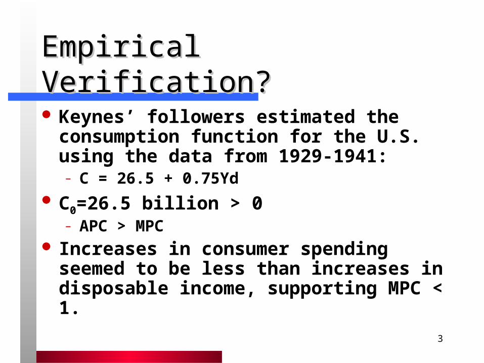
Keynes’ followers estimated the consumption function for the U.S. using the data from 1929-1941:– C = 26.5 + 0.75Yd

C0=26.5 billion > 0– APC > MPC

Increases in consumer spending seemed to be less than increases in disposable income, supporting MPC < 1.

4

Kuznets’ Consumption DataKuznets’ Consumption Data

Kuznets, Simon. Uses of National Income in Peace and War, Occasional Paper 6. NY: NBER, 1942.

Time series estimates of consumption and national income

Overlapping decades 1879-1938, 5 year steps Each estimate is a decade average

Kuznets, Simon. National Product Since 1869. NY: NBER, 1946.

Extended data backward to 1869.

5

Kuznets’ Study (1)Kuznets’ Study (1)

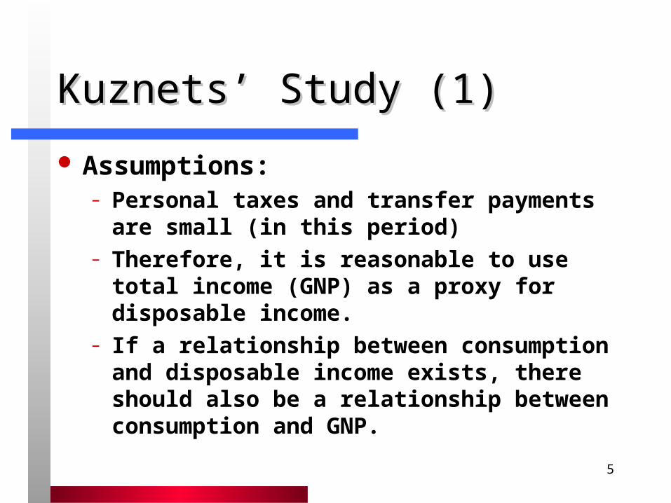
Assumptions:– Personal taxes and transfer payments are

small (in this period)– Therefore, it is reasonable to use total income

(GNP) as a proxy for disposable income.– If a relationship between consumption and

disposable income exists, there should also be a relationship between consumption and GNP.

6

Kuznets’ Study (2)Kuznets’ Study (2)

(1946 study) Between 1869-1938, real income expanded to seven (7) times its 1869 level ($9.3 billion to $69 billion)

But the average propensity to consume ranged between 0.838 and 0.898.

That is, APC did not vary significantly in the face of vastly expanding income.

Results:

Problem!

7

Kuznets’ Study (3)Kuznets’ Study (3)Years Y C C/Y

1869-78 9.3 8.1 0.87

1874-83 13.6 11.6 0.85

1879-88 17.9 15.3 0.85

1884-93 21.0 17.7 0.84

1889-98 24.2 20.2 0.83

1894-1903 29.8 25.4 0.85

1899-1908 37.3 32.3 0.87

1904-13 45.0 39.1 0.87

1909-18 50.6 44.0 0.87

1914-23 57.3 50.7 0.88

1919-28 69.0 62.0 0.90

1924-33 73.3 68.9 0.94

1929-38 72.0 71.0 0.99

8

Second FailureSecond Failure

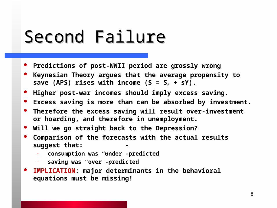
Predictions of post-WWII period are grossly wrong Keynesian Theory argues that the average propensity to save

(APS) rises with income (S = S0 + sY). Higher post-war incomes should imply excess saving. Excess saving is more than can be absorbed by investment. Therefore the excess saving will result over-investment or

hoarding, and therefore in unemployment. Will we go straight back to the Depression? Comparison of the forecasts with the actual results suggest that:

– consumption was “under”-predicted– saving was “over”-predicted

IMPLICATION: major determinants in the behavioral equations must be missing!

9

10

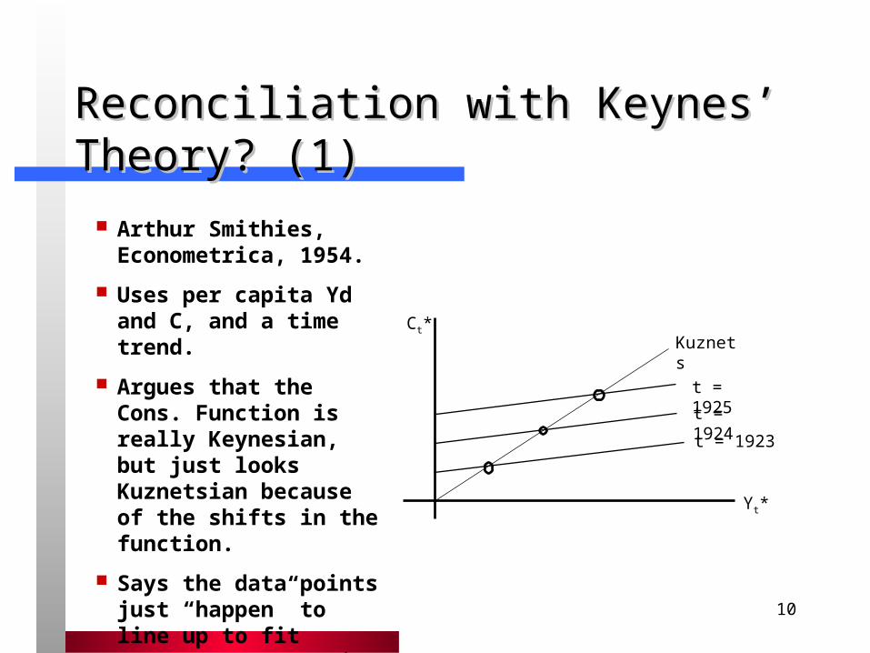
Reconciliation with Keynes’ Theory? (1)Reconciliation with Keynes’ Theory? (1)

t = 1923

t = 1924

t = 1925

Kuznets

Yt*

Ct*

Arthur Smithies, Econometrica, 1954.

Uses per capita Yd and C, and a time trend.

Argues that the Cons. Function is really Keynesian, but just looks Kuznetsian because of the shifts in the function.

Says the data points just “happen” to line up to fit Kuznets’ consumption function.

11

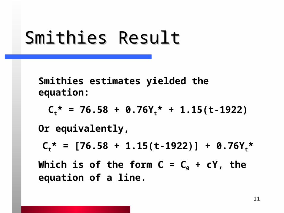
Smithies ResultSmithies Result

Smithies estimates yielded the equation:

Ct* = 76.58 + 0.76Yt* + 1.15(t-1922)

Or equivalently,

Ct* = [76.58 + 1.15(t-1922)] + 0.76Yt*

Which is of the form C = C0 + cY, the equation of a line.

12

Reconciliation (2)Reconciliation (2)

Reasons for shifts: Migration of people from farms to cities

(must buy goods) Shift in distribution toward greater

equality (poorer save less) Rise in the perceived “standard” of living

(luxuries become necessities) For these reasons each agent (per capita)

should increase his or her consumption.

13

Modigliani gets involvedModigliani gets involved

Modigliani, Franco. “Fluctuations in the saving-income ration: a problem in economic forecasting, “ in Studies in Income and Wealth vol. 11, Conference on Research in Income and Wealth. NY: NBER, 1949, pp. 373-378.

When Franco Modigliani (1949) estimates Smithies’ relation over a different time period, the analysis completely breaks down.

But, Modigliani is hooked...

14

More Problems

15

16

Habit Persistence TheoryHabit Persistence Theory

Note: Duesenberry and Modigliani both presented similar results at the Econometric Society Meeting of 1947.

Duesenberry (1947) noted that in 1935 dissaving grew as a percentage of income.

– Dissaving was greater in1935 than in the relatively prosperous year 1941.

– Why? Households must sacrifice saving to “defend” (attempt to maintain) their standard of living.

Duesenberry and Modigliani can reconcile the short-run and long-run consumption functions, but cannot explain the negative relationship betweem current income and consumption that sometimes occurs.

17

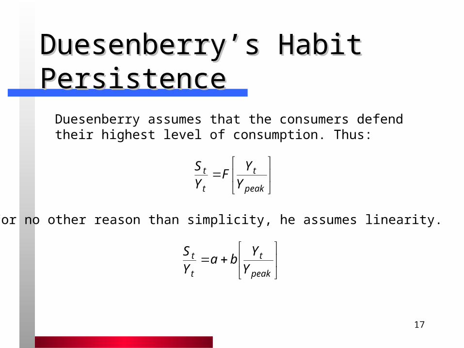
Duesenberry’s Habit PersistenceDuesenberry’s Habit Persistence

Duesenberry assumes that the consumers defend their highest level of consumption. Thus:

peak

t

t

t

YY

FYS

For no other reason than simplicity, he assumes linearity.

peak

t

t

t

YY

baYS

18

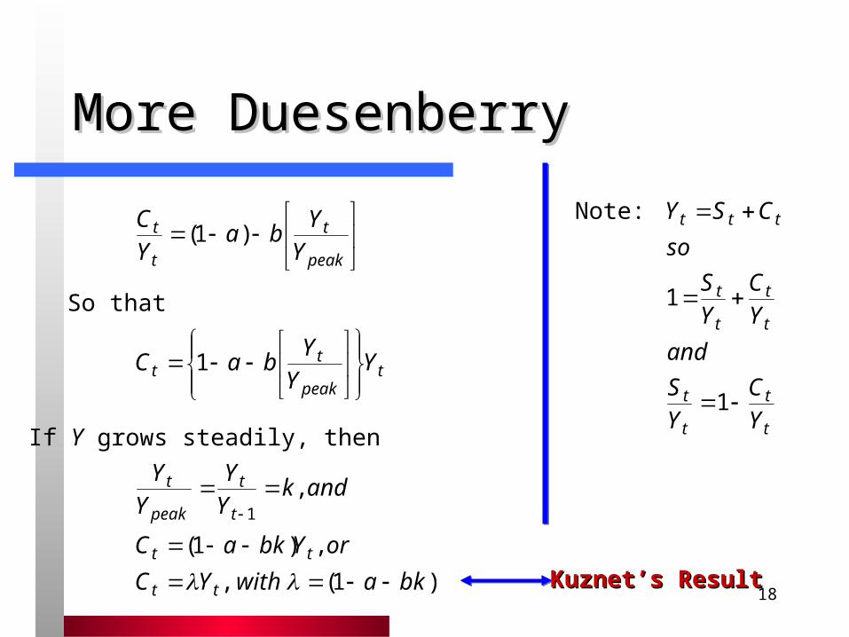
More DuesenberryMore Duesenberry

Note:

t

t

t

t

t

t

t

t

ttt

YC

YS

and

YC

YS

so

CSY

1

1

peak

t

t

t

YY

baYC

)1(

So that

tpeak

tt Y

YY

baC

1

If Y grows steadily, then

)1(,

,)1(

,1

bkawithYC

orYbkaC

andkYY

YY

tt

tt

t

t

peak

t

Kuznet’s ResultKuznet’s Result

19

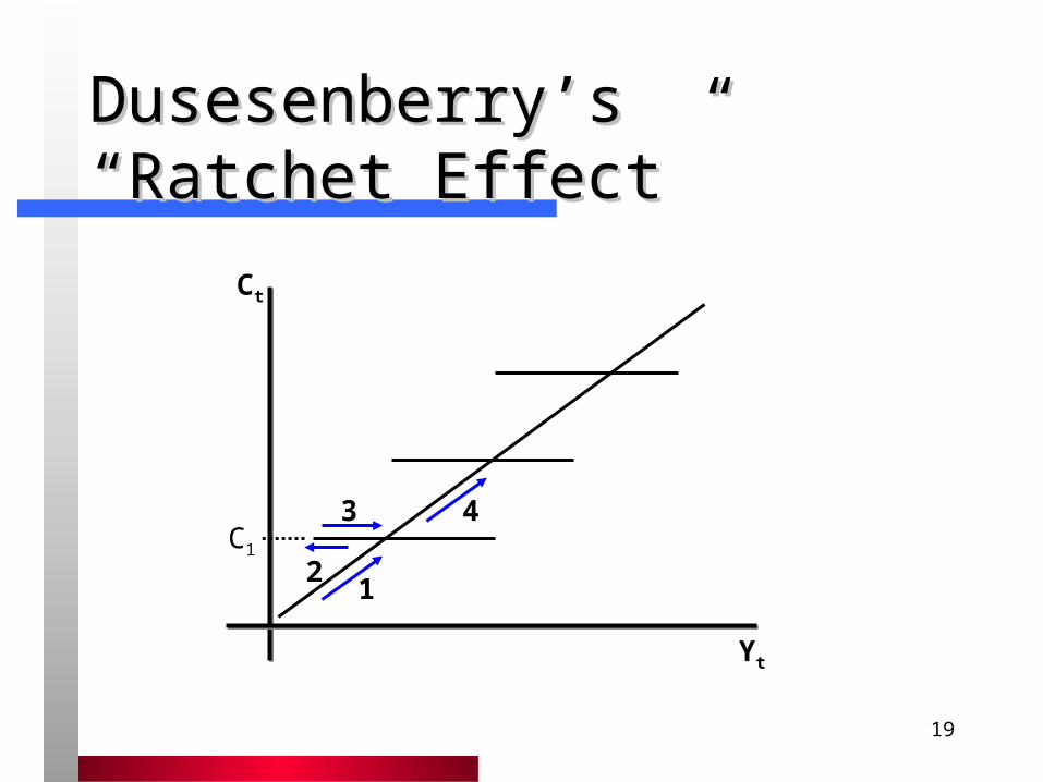
Dusesenberry’s “Ratchet Effect”Dusesenberry’s “Ratchet Effect”

Ct

Yt

12

3 4C1

20

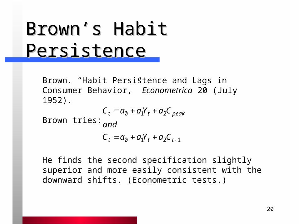
Brown’s Habit PersistenceBrown’s Habit Persistence

Brown. “Habit Persistence and Lags in Consumer Behavior,” Econometrica 20 (July 1952).

Brown tries:

1210

210

ttt

peaktt

CaYaaC

and

CaYaaC

He finds the second specification slightly superior and more easily consistent with the downward shifts. (Econometric tests.)

21

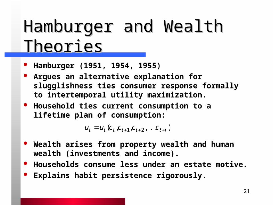
Hamburger and Wealth TheoriesHamburger and Wealth Theories

Hamburger (1951, 1954, 1955) Argues an alternative explanation for slugglishness ties

consumer response formally to intertemporal utility maximization.

Household ties current consumption to a lifetime plan of consumption:

Wealth arises from property wealth and human wealth (investments and income).

Households consume less under an estate motive. Explains habit persistence rigorously.

),...,,,( 21 itttttt ccccuu

22

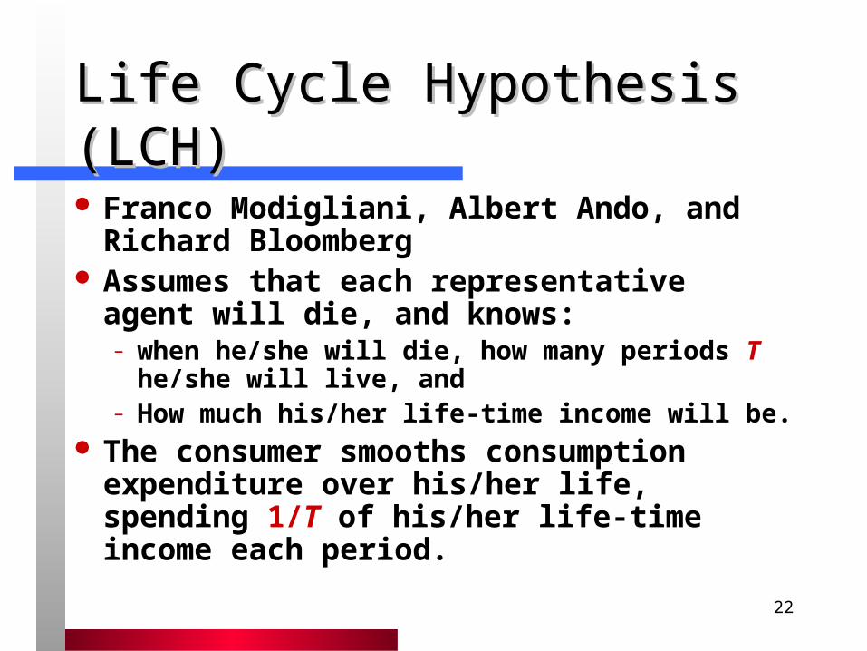
Life Cycle Hypothesis (LCH)Life Cycle Hypothesis (LCH)

Franco Modigliani, Albert Ando, and Richard Bloomberg

Assumes that each representative agent will die, and knows:– when he/she will die, how many periods T

he/she will live, and– How much his/her life-time income will be.

The consumer smooths consumption expenditure over his/her life, spending 1/T of his/her life-time income each period.

23

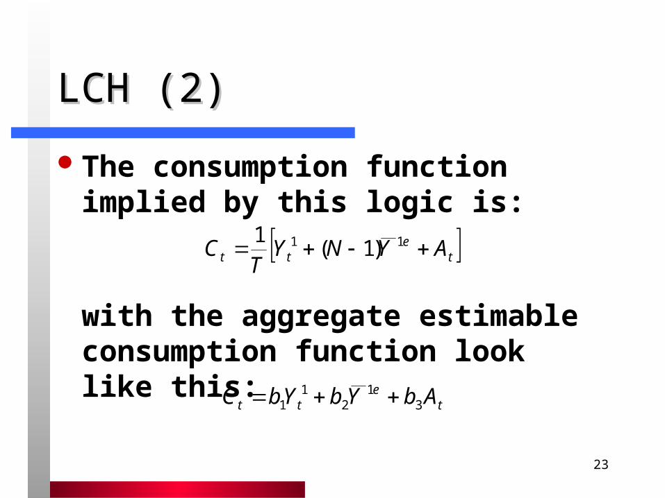
LCH (2)LCH (2)

The consumption function implied by this logic is:

with the aggregate estimable consumption function look like this:

tett AYNY

TC 11 )1(

1

te

tt AbYbYbC 31

21

1

24

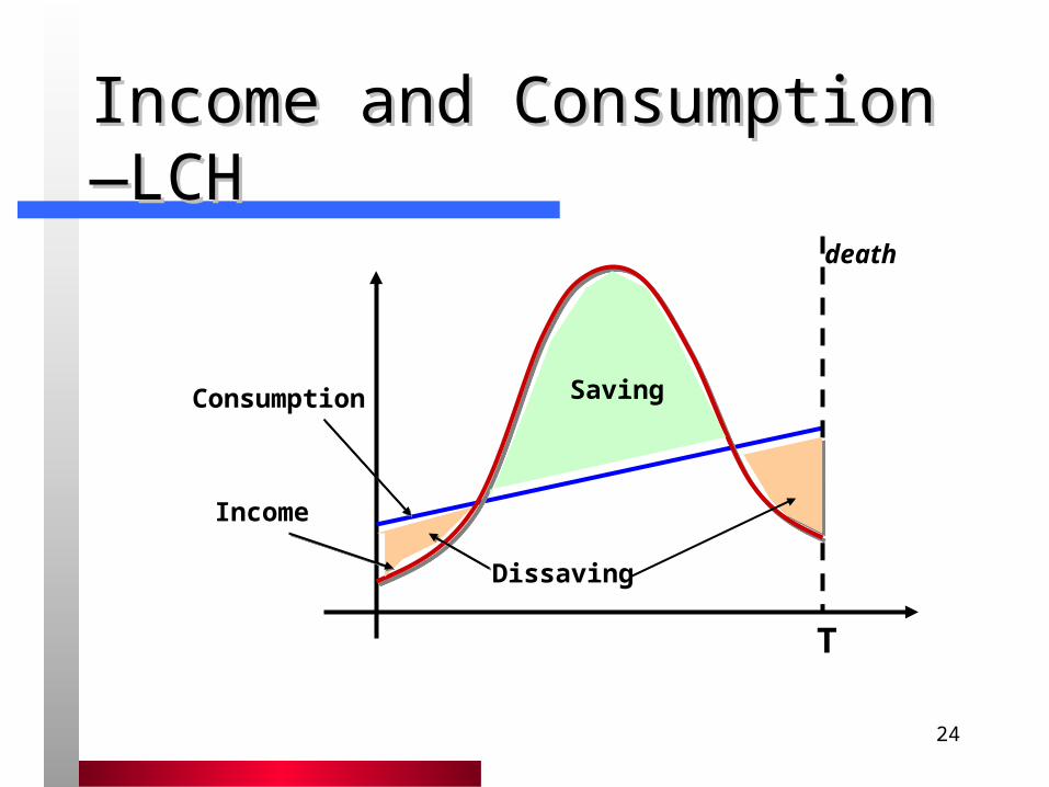
Income and Consumption—LCH Income and Consumption—LCH

death

T

Consumption

Income

Dissaving

Saving

25

Testing the LCHTesting the LCH

If the function form looks like this:

Ando and Modigliani argue that expected future labor income is proportional to current income, so that the function can be reduced to:

When they estimate this function, they get:

te

tt AbYbYbC 31

21

1

ttt AbYbbC 31

21 )(

ttt AYC 06.072.0 1

26

Criticisms of LCHCriticisms of LCH

The households, at all times, have a definite, conscious vision of:

– The family’s future size and composition, including the life expectancy of each member,

– The entire lifetime profile of the labor income of each member—after the applicable taxes,

– The present and future extent and terms of any credit available, and

– The future emergencies, opportunities, and social pressures which might affect its consumption spending.

It does not take into account liquidity constraints.

27

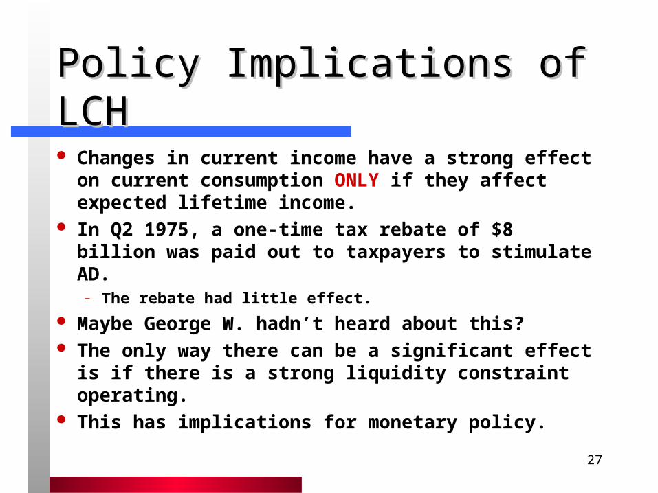
Policy Implications of LCHPolicy Implications of LCH

Changes in current income have a strong effect on current consumption ONLY if they affect expected lifetime income.

In Q2 1975, a one-time tax rebate of $8 billion was paid out to taxpayers to stimulate AD.

– The rebate had little effect.

Maybe George W. hadn’t heard about this? The only way there can be a significant effect is if

there is a strong liquidity constraint operating. This has implications for monetary policy.

28

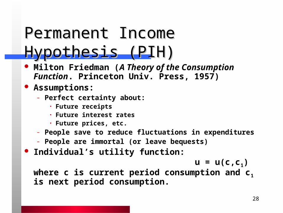
Permanent Income Hypothesis (PIH)Permanent Income Hypothesis (PIH) Milton Friedman (A Theory of the Consumption

Function. Princeton Univ. Press, 1957) Assumptions:

– Perfect certainty about:• Future receipts• Future interest rates• Future prices, etc.

– People save to reduce fluctuations in expenditures– People are immortal (or leave bequests)

Individual’s utility function: u = u(c,c1)where c is current period consumption and c1 is next period consumption.

29

PIH, ContinuedPIH, Continued

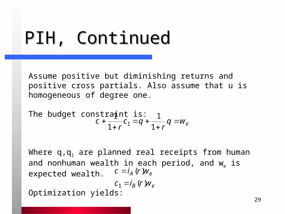
Assume positive but diminishing returns and positive cross partials. Also assume that u is homogeneous of degree one.

The budget constraint is:

Where q,q1 are planned real receipts from human and nonhuman wealth in each period, and we is expected wealth.

Optimization yields:

ewqr

qcr

c

1

11

11

eB

eA

wric

wric

)(

)(

1

30

PIH, ContinuedPIH, Continued

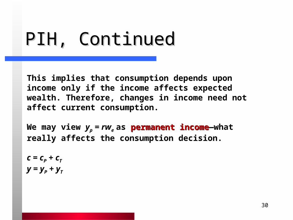
This implies that consumption depends upon income only if the income affects expected wealth. Therefore, changes in income need not affect current consumption.

We may view yp = rwe as permanent incomepermanent income—what really affects the consumption decision.

c = cP + cT

y = yP + yT

31

PIH, ContinuedPIH, Continued

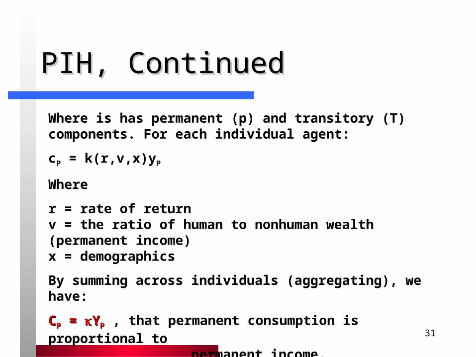
Where is has permanent (p) and transitory (T) components. For each individual agent:

cP = k(r,v,x)yP

Where

r = rate of returnv = the ratio of human to nonhuman wealth (permanent income)x = demographics

By summing across individuals (aggregating), we have:

CCPP = = YYPP , that permanent consumption is proportional to permanent income.

32

PIH, ContinuedPIH, Continued

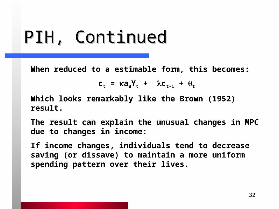
When reduced to a estimable form, this becomes:

ct = a0Yt + ct-1 + t

Which looks remarkably like the Brown (1952) result.

The result can explain the unusual changes in MPC due to changes in income:

If income changes, individuals tend to decrease saving (or dissave) to maintain a more uniform spending pattern over their lives.

33

PIH (2)PIH (2)

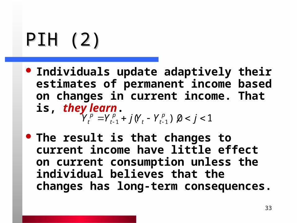
Individuals update adaptively their estimates of permanent income based on changes in current income. That is, they learn.

The result is that changes to current income have little effect on current consumption unless the individual believes that the changes has long-term consequences.

10),( 11 jYYjYY ptt

pt

pt

34

Investment SpendingInvestment Spending

Investment is the change in the capital stock– In,t = Kt – Kt-1 = Net Investment

– Ig,t = Kt – Kt-1 – Kt = Gross Investment (Kt is depreciation)

– I = I(r,E) = I(r)What about the expectations term?

35

The Accelerator Model (1)The Accelerator Model (1)

Attempts to capture some measure of current business conditions (growth of the economy or lack of it), and use that to explain the level of investment.

36

Accelerator Model (2)Accelerator Model (2)

The desired capital stock is proportional to the level of output:

Investment is the process of moving from the current level of capital to a desired level:

We assume that whatever the capital stock ended up being last period was the level of capital that businesses actually wanted:

tdt YK

1, tdttn KKI

111 tdtt YKK

37

Accelerator Model (3)Accelerator Model (3)

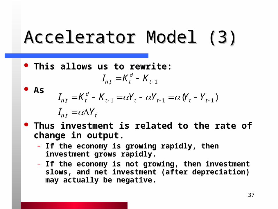
This allows us to rewrite:

As

Thus investment is related to the rate of change in output.

– If the economy is growing rapidly, then investment grows rapidly.

– If the economy is not growing, then investment slows, and net investment (after depreciation) may actually be negative.

1, tdttn KKI

ttn

tttttdttn

YI

YYYYKKI

,

111, )(

38

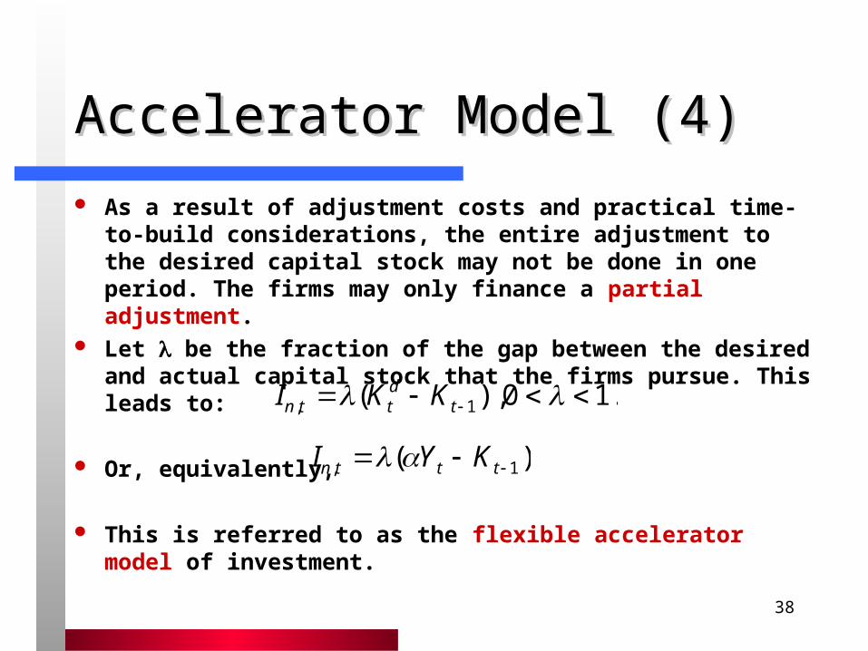
Accelerator Model (4)Accelerator Model (4)

As a result of adjustment costs and practical time-to-build considerations, the entire adjustment to the desired capital stock may not be done in one period. The firms may only finance a partial adjustment.

Let be the fraction of the gap between the desired and actual capital stock that the firms pursue. This leads to:

Or, equivalently,

This is referred to as the flexible accelerator model of investment.

.10),( 1, tdttn KKI

)( 1, tttn KYI

39

Cost of Capital ApproachCost of Capital Approach

MEC all over again? Recall that Keynes argued that business

decision makers compare the expected revenue stream from the new capital to the cost of capital.

The user cost of capital is the total cost to the firm of employing an additional unit of capital for one period.– The new capital might be funded by borrowing,

selling stock shares, retained earnings, etc.

40

Cost of Capital Approach (2)Cost of Capital Approach (2)

This suggests an investment function of the form:

If a firm invested its retained earnings or monies raised by selling stock shares, it could earn the current interest rate. So this must be the opportunity cost we are looking for.

Investment must be related to this interest rate—specifically, to the real interest rate , where:

),,( 1, ttttn KCCYII

epr

41

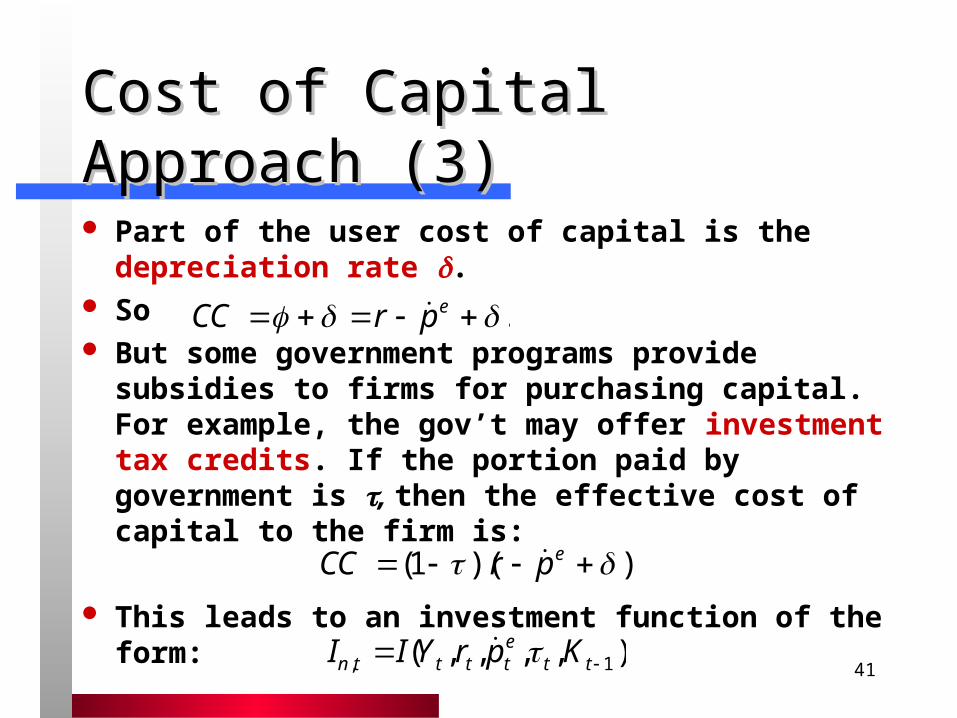
Cost of Capital Approach (3)Cost of Capital Approach (3)

Part of the user cost of capital is the depreciation rate .

So But some government programs provide subsidies

to firms for purchasing capital. For example, the gov’t may offer investment tax credits. If the portion paid by government is , then the effective cost of capital to the firm is:

This leads to an investment function of the form:

. eprCC

).)(1( eprCC

),,,,( 1, ttettttn KprYII