Embed Size (px)
Citation preview
27
Consumer Expenditure SurveyAnthology, 2005
.
U.S. Department of LaborU.S. Bureau of Labor Statistics
April 2005
Report 981
iii
Preface
This is the second in a series of reports presenting botharticles that discuss ongoing research and method-ological issues pertaining to the U.S. Bureau of Labor
Statistics (BLS) Consumer Expenditure Survey (CE) and ana-lytical articles using this survey’s data. The first report, Con-sumer Expenditure Survey Anthology, 2003, was publishedin September 2003. Future CE anthology reports will be pub-lished biennially, with the next report scheduled for publica-tion in 2006. The methodological articles included in thisreport are intended to provide data users with greater insightinto improvements in the survey, as well as issues that arefaced in collecting, processing, and publishing informationfrom such a complex survey. The analytical articles provideinformation on topics of interest using CE data.
This report was prepared in the Office of Prices and LivingConditions, Division of Consumer Expenditure Surveys(DCES), under the general direction of Steve Henderson,Chief of the Branch of Information and Analysis, and wasproduced and edited by John M. Rogers, Section Chief.Articles on research and methodology were contributed byJeanette Davis, Eric Figueroa, Lucilla Tan, and Nhien To ofthe Branch of Research and Program Development, andSylvia Johnson-Herring, Sharon Krieger, Sally Reyes-Morales,and David Swanson of the Division of Price Statistical Meth-ods. Analytical articles were contributed by Meaghan Duetsch,
Abby Duly, George Janini, Laura Paszkiewicz, and MarkVendemia of the Branch of Information and Analysis.
BLS makes CE data available in news releases, reports,and articles in the Monthly Labor Review, as well as on CD-ROMs and on the Internet. A biennial report includes stan-dard tables of recent survey data, a discussion of expenditurechanges, and a description of the survey and its methods.Current and historical CE tables classified by standard demo-graphic variables are available at the BLS Internet site http://www.bls.gov/cex. This site also provides other survey infor-mation, including answers to frequently asked questions, aglossary of terms, order forms for survey products, andMonthly Labor Review and other research articles.
The material that follows is divided into two sections: Part1 includes articles on survey research and methodology, andPart 2 presents analysis of topics of interest based on CEdata. An appendix includes a general description of the sur-vey and its methods and a glossary of terms.
Sensory-impaired individuals may obtain information onthis publication upon request. Voice phone: (202) 691-5200,Federal Relay Service: 1-800-877-8339. The material pre-sented is in the public domain and, with appropriate credit,may be reproduced without permission. Cover photo fromthe Library of Congress. For further information, call (202)691-6900.
v
Part I. Survey Research and Methodology ................................................................................................. 1
Is a user-friendly diary more effective? Findings from a field test ............................................................................ 2A new Diary Survey questionnaire, designed to be more user-friendly, was tested to see how well itperformed compared to the questionnaire being used.Eric Figueroa, Jeanette Davis, Sally Reyes-Morales, Nhien To, and Lucilla Tan
The efficacy of cues in an expenditure diary ................................................................................................................ 9A cognitive study tested whether adding cues to the recording pages of the new Diary Survey questionnairewould result in more detailed reporting by respondents.Nhien To, Eric Figueroa, and Lucilla Tan
Characteristics of nonresponders in the Consumer Expenditure Quarterly Interview Survey ................................ 18The characteristics of nonresponder consumer units were examined. The most common reason given fornot participating in the survey was “refusal.”Sally Reyes-Morales
Determining area sample sizes for the Consumer Expenditure Survey ..................................................................... 24A new, automated method of allocating the nationwide Consumer Expenditure Survey sample to individualgeographic areas was developed.Sylvia Johnson-Herring, Sharon Krieger, and David Swanson
Part II. Analyses Using Survey Data ............................................................................................................. 30
From AFDC to TANF: Have the new public assistance laws affected consumer spending of recipients? ................. 31There have been significant changes in the spending patterns of welfare recipients since the enactment ofwelfare reform legislation in 1996. Some changes follow trends in the non-welfare population, whereasothers are unique to welfare recipients.Laura Paszkiewicz
Spending patterns of older consumers raising a child ................................................................................................. 45The demographic characteristics and spending patterns of older consumer units raising children aredifferent both from those of their generation who have no children at home and from younger consumerunits raising children.Abby Duly
Tobacco expenditures by education, occupation, and age ............................................................................................. 51Average annual expenditures on tobacco continue to rise despite the heightened awareness of the healthissues involved, but expenditure increases are less than the increases in the prices of tobacco products.Spending patterns among various education, occupation, and age groups show marked differences.Mark Vendemia
Spending by singles ...................................................................................................................................................... 56Many differences in spending patterns between single women and single men can be explained bydifferences in characteristics between the two groups, particularly age. However, differences remaineven when controlling for age.Meaghan Duetsch
Trends in airfare expenditures ..................................................................................................................................... 61Spending on airline fares was at a peak prior to the September 11, 2001, terrorist attacks, fell sharply afterthat, and rebounded some by late 2002. Spending dropped off more for some age groups than for others,and the four regions of the country experienced different effects.George Janini
Appendix A: Description of the Consumer Expenditure Survey ................................................................................... 70
Contents
Page
Consumer Expenditure Survey Anthology, 2005 1
Part I.Survey Research and Methodology
2 Consumer Expenditure Survey Anthology, 2005
Is a User-Friendly DiaryMore Effective? Findingsfrom a Field Test
Eric Figueroa, Nhien To, and Lucilla Tan areeconomists in the Branch of Research andProgram Development, Division of Con-sumer Expenditure Surveys, Bureau of LaborStatistics.
Jeanette Davis is a senior economist in theBranch of Research and Program Develop-ment, Division of Consumer ExpenditureSurveys, Bureau of Labor Statistics.
Sally Reyes-Morales is a mathematical stat-istician in the Division of Price StatisticalMethods, Branch of Consumer ExpenditureSurveys, Bureau of Labor Statistics.
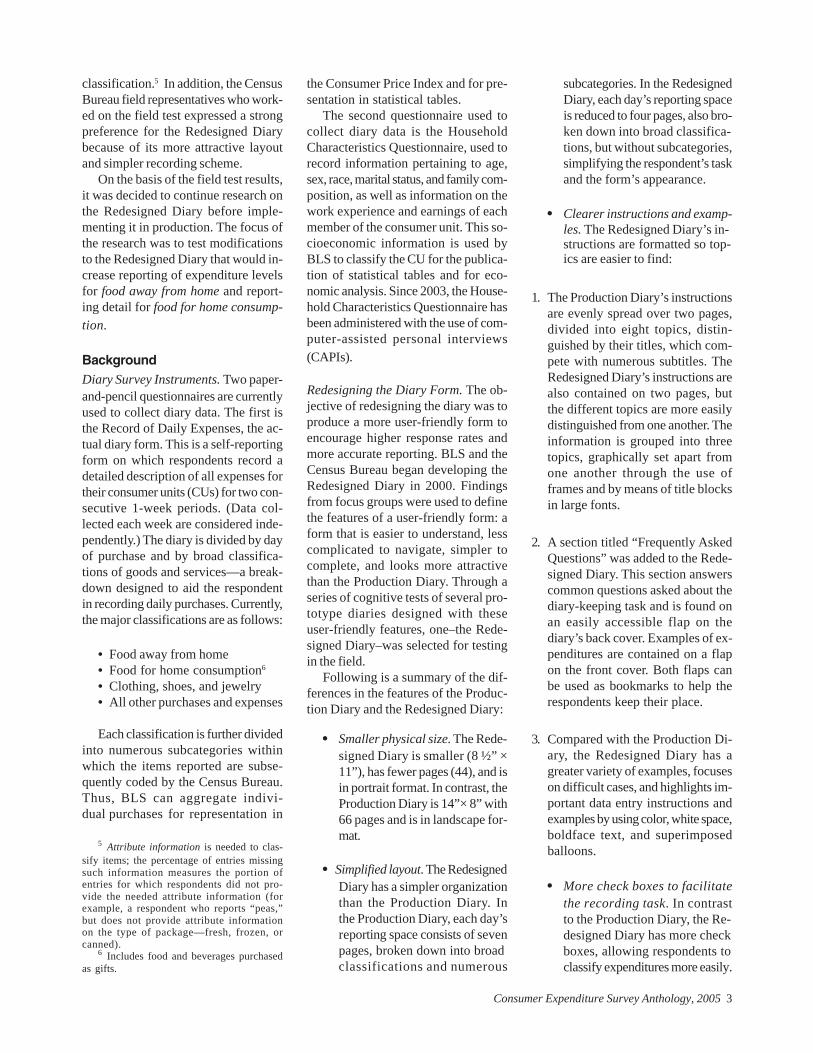
Diary surveys are often used tocollect information on dailyactivities such as consumer
spending. They are particularly usefulfor collecting daily records of small fre-quently purchased items, which arenormally difficult to recall.1 The Con-sumer Expenditure (CE) survey, spon-sored by the U.S. Bureau of LaborStatistics (BLS), with data collected bythe U.S. Census Bureau, uses a diarysurvey to collect data on weekly house-hold expenditures.
Recent efforts to improve the per-formance of the CE diary survey havefocused on designing a more user-friendly form. Such a form would havea simpler recording scheme and be moreattractive in appearance than the formcurrently used in production. Severalprototype diaries were developed andrefined with the use of feedback fromsurvey respondents, field interviewers,and program staff.2 On the basis of thisfeedback, CE management selected oneof the designs (the Redesigned Diary)for field testing. This diary was in-tended to stem declining response ratesand improve data quality by reducingrespondent’s burden associated with
the diary now used: the ProductionDiary. The Redesigned Diary is smallerand shorter than the Production Diary,has a simpler organization, and high-lights important instructions and ex-amples.
The Redesigned Diary was testedin the field from October through De-cember of 2002.3 The primary objectiveof this field test was to compare theresponse rates and data quality ob-tained from the Redesigned Diary withthose obtained from the ProductionDiary. The results showed no statisti-cally significant difference between di-ary forms in completion response ratesand only a few significant differencesin expenditure means and allocationrates. (The latter measure the propor-tion of expenditures requiring furtherprocessing because they are reportedwith insufficient detail.4 )
However, the Redesigned Diary per-formed statistically significantly betterthan the Production Diary in a majorityof tests pertaining to the collection ofitem attribute information needed for
3 A field test is designed to reproduce datacollection conditions as closely as possibleto those in the production environment.
4 Allocation is an adjustment performedon expenditure entries that do not identifyindividual items at the required level of detail(for example, a report that says “groceries$150,” rather than listing the specific itemspurchased and the price of each). This typeof entry requires additional processing to as-sign the aggregate expenditure to target items.
ERIC FIGUEROANHIEN TOLUCILLA TANJEANETTE DAVISSALLY REYES-MORALES
1 S. Sudman and N. Bradburn, Asking Ques-tions, (San Francisco, Jossey Bass Publishers,1982).
2 J. Davis, L. Stinson, and N. To, “Creat-ing a ‘User-Friendly’ Expenditure Diary,”Consumer Expenditure Survey Anthology(Bureau of Labor Statistics, 2003), Report967, p. 3.
Consumer Expenditure Survey Anthology, 2005 3
classification.5 In addition, the CensusBureau field representatives who work-ed on the field test expressed a strongpreference for the Redesigned Diarybecause of its more attractive layoutand simpler recording scheme.
On the basis of the field test results,it was decided to continue research onthe Redesigned Diary before imple-menting it in production. The focus ofthe research was to test modificationsto the Redesigned Diary that would in-crease reporting of expenditure levelsfor food away from home and report-ing detail for food for home consump-tion.
BackgroundDiary Survey Instruments. Two paper-and-pencil questionnaires are currentlyused to collect diary data. The first isthe Record of Daily Expenses, the ac-tual diary form. This is a self-reportingform on which respondents record adetailed description of all expenses fortheir consumer units (CUs) for two con-secutive 1-week periods. (Data col-lected each week are considered inde-pendently.) The diary is divided by dayof purchase and by broad classifica-tions of goods and services—a break-down designed to aid the respondentin recording daily purchases. Currently,the major classifications are as follows:
• Food away from home• Food for home consumption6
• Clothing, shoes, and jewelry• All other purchases and expenses
Each classification is further dividedinto numerous subcategories withinwhich the items reported are subse-quently coded by the Census Bureau.Thus, BLS can aggregate indivi-dual purchases for representation in
the Consumer Price Index and for pre-sentation in statistical tables.
The second questionnaire used tocollect diary data is the HouseholdCharacteristics Questionnaire, used torecord information pertaining to age,sex, race, marital status, and family com-position, as well as information on thework experience and earnings of eachmember of the consumer unit. This so-cioeconomic information is used byBLS to classify the CU for the publica-tion of statistical tables and for eco-nomic analysis. Since 2003, the House-hold Characteristics Questionnaire hasbeen administered with the use of com-puter-assisted personal interviews(CAPIs).
Redesigning the Diary Form. The ob-jective of redesigning the diary was toproduce a more user-friendly form toencourage higher response rates andmore accurate reporting. BLS and theCensus Bureau began developing theRedesigned Diary in 2000. Findingsfrom focus groups were used to definethe features of a user-friendly form: aform that is easier to understand, lesscomplicated to navigate, simpler tocomplete, and looks more attractivethan the Production Diary. Through aseries of cognitive tests of several pro-totype diaries designed with theseuser-friendly features, one–the Rede-signed Diary–was selected for testingin the field.
Following is a summary of the dif-ferences in the features of the Produc-tion Diary and the Redesigned Diary:
• Smaller physical size. The Rede-signed Diary is smaller (8 ½” ×11”), has fewer pages (44), and isin portrait format. In contrast, theProduction Diary is 14”× 8” with66 pages and is in landscape for-mat.
• Simplified layout. The RedesignedDiary has a simpler organizationthan the Production Diary. Inthe Production Diary, each day’sreporting space consists of sevenpages, broken down into broadclassifications and numerous
subcategories. In the RedesignedDiary, each day’s reporting spaceis reduced to four pages, also bro-ken down into broad classifica-tions, but without subcategories,simplifying the respondent’s taskand the form’s appearance.
• Clearer instructions and examp-les. The Redesigned Diary’s in-structions are formatted so top-ics are easier to find:
1. The Production Diary’s instructionsare evenly spread over two pages,divided into eight topics, distin-guished by their titles, which com-pete with numerous subtitles. TheRedesigned Diary’s instructions arealso contained on two pages, butthe different topics are more easilydistinguished from one another. Theinformation is grouped into threetopics, graphically set apart fromone another through the use offrames and by means of title blocksin large fonts.
2. A section titled “Frequently AskedQuestions” was added to the Rede-signed Diary. This section answerscommon questions asked about thediary-keeping task and is found onan easily accessible flap on thediary’s back cover. Examples of ex-penditures are contained on a flapon the front cover. Both flaps canbe used as bookmarks to help therespondents keep their place.
3. Compared with the Production Di-ary, the Redesigned Diary has agreater variety of examples, focuseson difficult cases, and highlights im-portant data entry instructions andexamples by using color, white space,boldface text, and superimposedballoons.
• More check boxes to facilitatethe recording task. In contrastto the Production Diary, the Re-designed Diary has more checkboxes, allowing respondents toclassify expenditures more easily.
5 Attribute information is needed to clas-sify items; the percentage of entries missingsuch information measures the portion ofentries for which respondents did not pro-vide the needed attribute information (forexample, a respondent who reports “peas,”but does not provide attribute informationon the type of package—fresh, frozen, orcanned).
6 Includes food and beverages purchasedas gifts.
4 Consumer Expenditure Survey Anthology, 2005
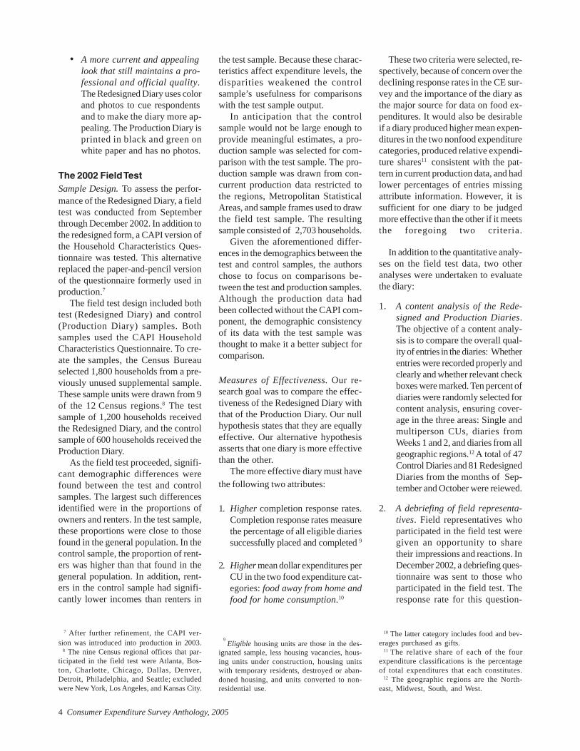
• A more current and appealinglook that still maintains a pro-fessional and official quality.The Redesigned Diary uses colorand photos to cue respondentsand to make the diary more ap-pealing. The Production Diary isprinted in black and green onwhite paper and has no photos.
The 2002 Field TestSample Design. To assess the perfor-mance of the Redesigned Diary, a fieldtest was conducted from Septemberthrough December 2002. In addition tothe redesigned form, a CAPI version ofthe Household Characteristics Ques-tionnaire was tested. This alternativereplaced the paper-and-pencil versionof the questionnaire formerly used inproduction.7
The field test design included bothtest (Redesigned Diary) and control(Production Diary) samples. Bothsamples used the CAPI HouseholdCharacteristics Questionnaire. To cre-ate the samples, the Census Bureauselected 1,800 households from a pre-viously unused supplemental sample.These sample units were drawn from 9of the 12 Census regions.8 The testsample of 1,200 households receivedthe Redesigned Diary, and the controlsample of 600 households received theProduction Diary.
As the field test proceeded, signifi-cant demographic differences werefound between the test and controlsamples. The largest such differencesidentified were in the proportions ofowners and renters. In the test sample,these proportions were close to thosefound in the general population. In thecontrol sample, the proportion of rent-ers was higher than that found in thegeneral population. In addition, rent-ers in the control sample had signifi-cantly lower incomes than renters in
the test sample. Because these charac-teristics affect expenditure levels, thedisparities weakened the controlsample’s usefulness for comparisonswith the test sample output.
In anticipation that the controlsample would not be large enough toprovide meaningful estimates, a pro-duction sample was selected for com-parison with the test sample. The pro-duction sample was drawn from con-current production data restricted tothe regions, Metropolitan StatisticalAreas, and sample frames used to drawthe field test sample. The resultingsample consisted of 2,703 households.
Given the aforementioned differ-ences in the demographics between thetest and control samples, the authorschose to focus on comparisons be-tween the test and production samples.Although the production data hadbeen collected without the CAPI com-ponent, the demographic consistencyof its data with the test sample wasthought to make it a better subject forcomparison.
Measures of Effectiveness. Our re-search goal was to compare the effec-tiveness of the Redesigned Diary withthat of the Production Diary. Our nullhypothesis states that they are equallyeffective. Our alternative hypothesisasserts that one diary is more effectivethan the other.
The more effective diary must havethe following two attributes:
1. Higher completion response rates.Completion response rates measurethe percentage of all eligible diariessuccessfully placed and completed 9
2. Higher mean dollar expenditures perCU in the two food expenditure cat-egories: food away from home andfood for home consumption.10
7 After further refinement, the CAPI ver-sion was introduced into production in 2003.
8 The nine Census regional offices that par-ticipated in the field test were Atlanta, Bos-ton, Charlotte, Chicago, Dallas, Denver,Detroit, Philadelphia, and Seattle; excludedwere New York, Los Angeles, and Kansas City.
These two criteria were selected, re-spectively, because of concern over thedeclining response rates in the CE sur-vey and the importance of the diary asthe major source for data on food ex-penditures. It would also be desirableif a diary produced higher mean expen-ditures in the two nonfood expenditurecategories, produced relative expendi-ture shares11 consistent with the pat-tern in current production data, and hadlower percentages of entries missingattribute information. However, it issufficient for one diary to be judgedmore effective than the other if it meetsthe foregoing two criteria.
In addition to the quantitative analy-ses on the field test data, two otheranalyses were undertaken to evaluatethe diary:
1. A content analysis of the Rede-signed and Production Diaries.The objective of a content analy-sis is to compare the overall qual-ity of entries in the diaries: Whetherentries were recorded properly andclearly and whether relevant checkboxes were marked. Ten percent ofdiaries were randomly selected forcontent analysis, ensuring cover-age in the three areas: Single andmultiperson CUs, diaries fromWeeks 1 and 2, and diaries from allgeographic regions.12 A total of 47Control Diaries and 81 RedesignedDiaries from the months of Sep-tember and October were reiewed.
2. A debriefing of field representa-tives. Field representatives whoparticipated in the field test weregiven an opportunity to sharetheir impressions and reactions. InDecember 2002, a debriefing ques-tionnaire was sent to those whoparticipated in the field test. Theresponse rate for this question-
10 The latter category includes food and bev-erages purchased as gifts.
11 The relative share of each of the fourexpenditure classifications is the percentageof total expenditures that each constitutes.
12 The geographic regions are the North-east, Midwest, South, and West.
9Eligible housing units are those in the des-
ignated sample, less housing vacancies, hous-ing units under construction, housing unitswith temporary residents, destroyed or aban-doned housing, and units converted to non-residential use.
Consumer Expenditure Survey Anthology, 2005 5
naire was 86 percent. A total of 17field representatives representingthe 9 Census regional offices par-ticipated in a 1-day debriefing inJanuary 2003.
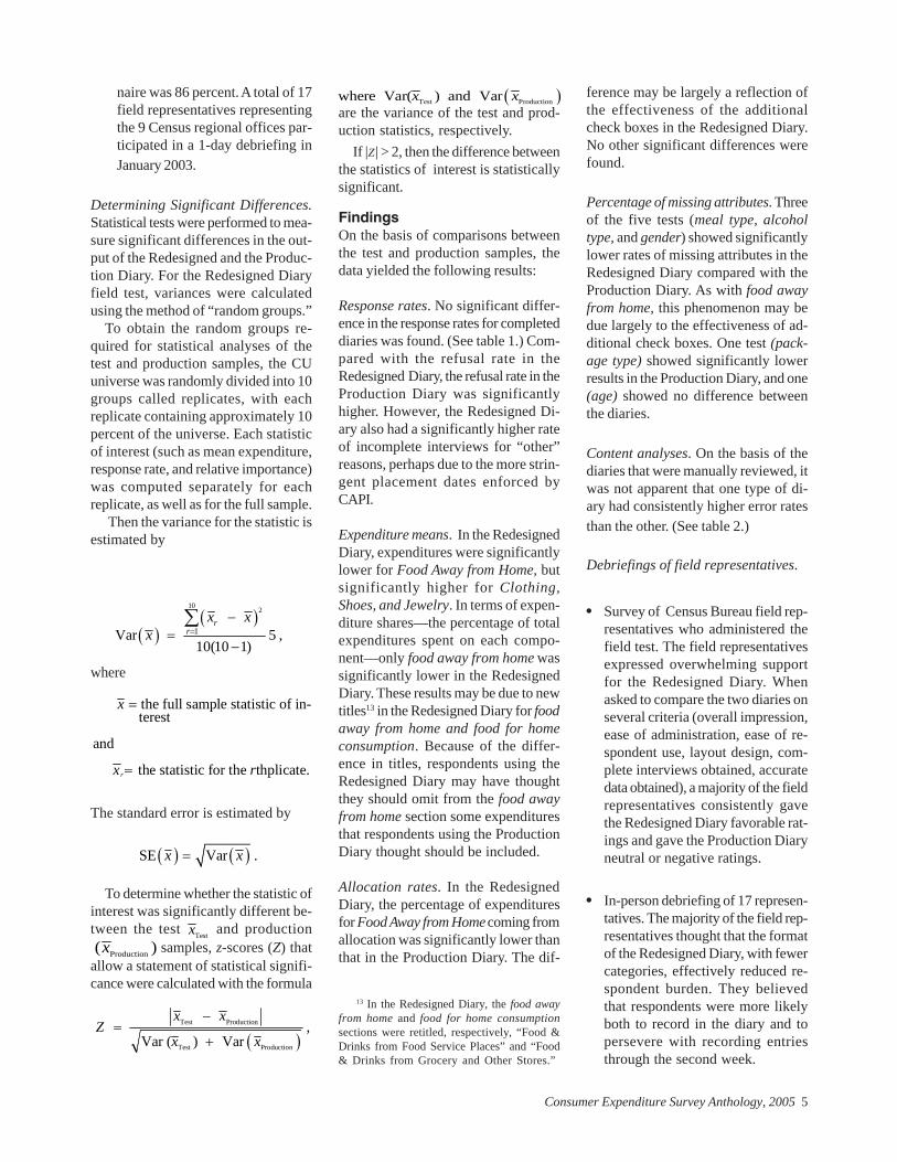
Determining Significant Differences.Statistical tests were performed to mea-sure significant differences in the out-put of the Redesigned and the Produc-tion Diary. For the Redesigned Diaryfield test, variances were calculatedusing the method of “random groups.”
To obtain the random groups re-quired for statistical analyses of thetest and production samples, the CUuniverse was randomly divided into 10groups called replicates, with eachreplicate containing approximately 10percent of the universe. Each statisticof interest (such as mean expenditure,response rate, and relative importance)was computed separately for eachreplicate, as well as for the full sample.
Then the variance for the statistic isestimated by
The standard error is estimated by
If |Z| > 2, then the difference betweenthe statistics of interest is statisticallysignificant.
FindingsOn the basis of comparisons betweenthe test and production samples, thedata yielded the following results:
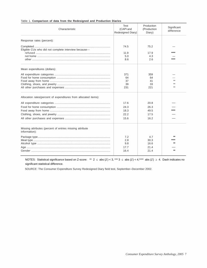
Response rates. No significant differ-ence in the response rates for completeddiaries was found. (See table 1.) Com-pared with the refusal rate in theRedesigned Diary, the refusal rate in theProduction Diary was significantlyhigher. However, the Redesigned Di-ary also had a significantly higher rateof incomplete interviews for “other”reasons, perhaps due to the more strin-gent placement dates enforced byCAPI.
Expenditure means. In the RedesignedDiary, expenditures were significantlylower for Food Away from Home, butsignificantly higher for Clothing,Shoes, and Jewelry. In terms of expen-diture shares—the percentage of totalexpenditures spent on each compo-nent—only food away from home wassignificantly lower in the RedesignedDiary. These results may be due to newtitles13 in the Redesigned Diary for foodaway from home and food for homeconsumption. Because of the differ-ence in titles, respondents using theRedesigned Diary may have thoughtthey should omit from the food awayfrom home section some expendituresthat respondents using the ProductionDiary thought should be included.
Allocation rates. In the RedesignedDiary, the percentage of expendituresfor Food Away from Home coming fromallocation was significantly lower thanthat in the Production Diary. The dif-
To determine whether the statistic ofinterest was significantly different be-tween the test and production samples, z-scores (Z) thatallow a statement of statistical signifi-cance were calculated with the formula
are the variance of the test and prod-uction statistics, respectively.
13 In the Redesigned Diary, the food awayfrom home and food for home consumptionsections were retitled, respectively, “Food &Drinks from Food Service Places” and “Food& Drinks from Grocery and Other Stores.”
ference may be largely a reflection ofthe effectiveness of the additionalcheck boxes in the Redesigned Diary.No other significant differences werefound.
Percentage of missing attributes. Threeof the five tests (meal type, alcoholtype, and gender) showed significantlylower rates of missing attributes in theRedesigned Diary compared with theProduction Diary. As with food awayfrom home, this phenomenon may bedue largely to the effectiveness of ad-ditional check boxes. One test (pack-age type) showed significantly lowerresults in the Production Diary, and one(age) showed no difference betweenthe diaries.
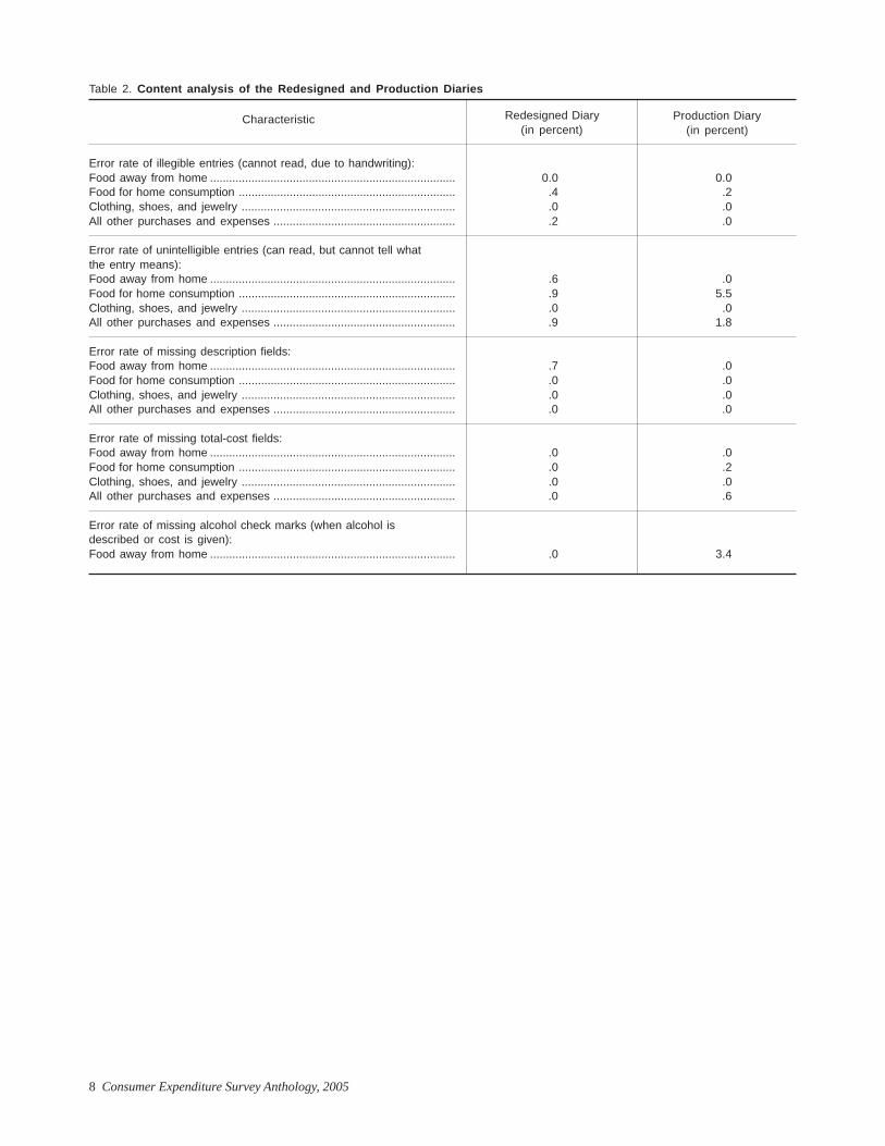
Content analyses. On the basis of thediaries that were manually reviewed, itwas not apparent that one type of di-ary had consistently higher error ratesthan the other. (See table 2.)
Debriefings of field representatives.
• Survey of Census Bureau field rep-resentatives who administered thefield test. The field representativesexpressed overwhelming supportfor the Redesigned Diary. Whenasked to compare the two diaries onseveral criteria (overall impression,ease of administration, ease of re-spondent use, layout design, com-plete interviews obtained, accuratedata obtained), a majority of the fieldrepresentatives consistently gavethe Redesigned Diary favorable rat-ings and gave the Production Diaryneutral or negative ratings.
• In-person debriefing of 17 represen-tatives. The majority of the field rep-resentatives thought that the formatof the Redesigned Diary, with fewercategories, effectively reduced re-spondent burden. They believedthat respondents were more likelyboth to record in the diary and topersevere with recording entriesthrough the second week.
( )( )
10 2
1Var 5 ,10(10 1)
rr
x xx =
−=
−
∑
where
( ) ( )SE Var .x x=
the full sample statistic of in-terest
and
the statistic for the thplicate.
x
x r
=
=
TestxProduction( )x
( )Test Production
Test Production
,Var ( ) Var
x xZ
x x
−=
+
( )Test Productionwhere Var( ) and Varx x
r
6 Consumer Expenditure Survey Anthology, 2005
ConclusionThe findings of the diary field test didnot allow us to reject the null hypoth-esis. Thus, both the Redesigned Diaryand the Production Diary are equallyeffective. No significant difference wasfound in the test of completion re-sponse rates. Results were mixed fortests of mean expenditures in the twofood categories: the Redesigned Diaryhad significantly lower expendituresthan the Production Diary had for foodaway from home, and there was no sig-nificant difference between the diariesin food for home consumption. Higherresults on both tests were necessaryfor either diary to be judged more ef-fective than the other.
The Redesigned Diary performedsignificantly better in a majority of tests
having to do with missing attributeinformation. Taking into account all testdifferences—whether significant ornot—we find that the Redesigned Di-ary produced higher expenditure meansand lower allocation rates in three ofthe four expenditure categories. In ad-dition, the field representatives whoworked on the field test expressed astrong preference for the RedesignedDiary.
Further ReasearchThe Redesigned Diary’s weak areasmerit additional research. The expendi-ture means in the food away from homesection were lower in the RedesignedDiary than in the Production Diary.Cognitive work is needed to determinewhether the titles used in each diary
are confusing to respondents, possib-ly leading to incorrect items being en-tered.
Additional research also is neededto develop effective cues to encour-age more detailed reporting in the foodfor home consumption, the clothing,shoes, and jewelry, and the all otherpurchases and expenses sections. Thecues should not be overwhelming oradd significant amounts of respondentburden.
The authors would like to acknowl-edge the following BLS employees whocontributed to this analysis: Jeff Blaha,Richard Dietz, Tammy Hagemeier,William Mockovak, Troy Olson, MaryLynn Schmidt, Linda Stinson, DavidSwanson, Clyde Tucker, and WolfWeber.
Consumer Expenditure Survey Anthology, 2005 7
Table 1. Comparison of data from the Redesigned and Production Diaries
Response rates (percent):
Completed ...................................................................................................... 74.5 75.2 —Eligible CUs who did not complete interview because—
refused .................................................................................................... 11.9 17.9 ****not home .................................................................................................. 5.0 4.3 —other ......................................................................................................... 8.6 2.6 ****
Mean expenditures (dollars):
All expenditure categories ........................................................................... 371 359 —Food for home consumption ........................................................................ 64 64 —Food away from home ................................................................................. 37 41 **Clothing, shoes, and jewelry ....................................................................... 39 33 **All other purchases and expenses ............................................................. 231 221 **
Allocation rates(percent of expenditures from allocated items):
All expenditure categories ........................................................................... 17.6 20.8 —Food for home consumption ........................................................................ 24.3 26.3 —Food away from home ................................................................................. 18.3 49.5 ****Clothing, shoes, and jewelry ....................................................................... 22.2 17.5 —All other purchases and expenses ............................................................. 15.6 16.2 —
Missing attributes (percent of entries missing attributeinformation):
Package type ................................................................................................. 7.2 4.7 **Meal type ....................................................................................................... 2.8 30.3 ****Alcohol type .................................................................................................. 9.8 16.6 **Age ................................................................................................................ 17.7 21.4 —Gender .......................................................................................................... 16.4 21.4 **
SOURCE: The Consumer Expenditure Survey Redesigned Diary field test, September–December 2002.
Test(CAPI and
Redesigned Diary)
Production(Production
Diary)
SignificantdifferenceCharacteristic
Z Z Z≤ ≤ ≥ NOTES: Statistical significance based on Z-score: ** 2 abs ( ) < 3, *** 3 abs ( ) < 4,**** abs ( ) 4. Dash indicates no significant statistical difference.
8 Consumer Expenditure Survey Anthology, 2005
Table 2. Content analysis of the Redesigned and Production Diaries
Error rate of illegible entries (cannot read, due to handwriting):Food away from home ............................................................................. 0.0 0.0Food for home consumption .................................................................... .4 .2Clothing, shoes, and jewelry ................................................................... .0 .0All other purchases and expenses ......................................................... .2 .0
Error rate of unintelligible entries (can read, but cannot tell whatthe entry means):Food away from home ............................................................................. .6 .0Food for home consumption .................................................................... .9 5.5Clothing, shoes, and jewelry ................................................................... .0 .0All other purchases and expenses ......................................................... .9 1.8
Error rate of missing description fields:Food away from home ............................................................................. .7 .0Food for home consumption .................................................................... .0 .0Clothing, shoes, and jewelry ................................................................... .0 .0All other purchases and expenses ......................................................... .0 .0
Error rate of missing total-cost fields:Food away from home ............................................................................. .0 .0Food for home consumption .................................................................... .0 .2Clothing, shoes, and jewelry ................................................................... .0 .0All other purchases and expenses ......................................................... .0 .6
Error rate of missing alcohol check marks (when alcohol isdescribed or cost is given):Food away from home ............................................................................. .0 3.4
Production Diary(in percent)
Redesigned Diary(in percent)
Characteristic
Consumer Expenditure Survey Anthology, 2005 9
The Efficacy of Cues in anExpenditure Diary
Nhien To, Eric Figueroa, and Lucilla Tan areresearch economists in the Branch of Re-search and Program Development, Divisionof Consumer Expenditure Surveys, Bureau ofLabor Statistics.
NHIEN TOERIC FIGUEROALUCILLA TAN In designing any survey, it is impor-
tant to provide respondents withclear instructions and examples.
Self-administered expenditure diariesoften use cues as examples, not onlyto aid recall, but also to prompt the re-spondent as to what types of expensesto record and how those expensesshould be recorded. This cognitivestudy investigates how cues should beused in an expenditure diary to instructrespondents to record their expensescompletely and accurately.
BackgroundThe Consumer Expenditure Diary (CED)Survey is a nationwide survey ofhouseholds used by the U.S. Bureauof Labor Statistics (BLS) to collect ex-penditures on small, frequently pur-chased items. The respondent is askedto record the household’s expenses for2 consecutive weeks. Depending onhow promptly the respondent recordsthe expenditures in the diary after in-curring them, various degrees of recallare involved in the task. To aid in re-call, diary forms are often organized intobroad categories (e.g., “Food andDrinks for Home Consumption” or“Clothing, Shoes, Jewelry, and Acces-sories”) and include cues that are ex-amples of expenditure items.
Over the years, the use of cues inthe CED has undergone a variety ofchanges. The first annual CED, imple-mented in 1980, was organized into five
broad expenditure categories that wererepeated for each day of the week, re-sulting in a diary that was 23 pageslong. There were 76 specific cues1 onthe recording pages for each day.
In 1991, a new version of the diary(the Current Diary) was introduced. Inthis version, the five broad expenditurecategories were further divided into 42subcategories (e.g., an “Eggs andDairy Products” subcategory withinthe “Food for Home Consumption”category). As a result, there were 305specific cues on the recording pagesfor each day. A field test conducted in1991 showed that, for items mentionedin the cues, the Current Diary yieldedhigher reporting rates with relativelyhigher reporting detail than did the 1980diary.2
Despite the Current Diary’s strongperformance in the field test, decliningresponse rates and diminishing dataquality during the 1990s led CED re-searchers to reexamine the diary andthe diary-keeping task. A previous testin 1985 had revealed some disadvan-
1 Specific cues are precise examples ofitems described with sufficient detail for cod-ing. For example, “powdered milk” and “wholemilk” are specific cues because they containenough information to be accurately coded.By contrast, “milk” is not a specific cue,because it does not specify the type of milk.
2 Silberstein, A.R., “Part-Set Cuing in Di-ary Surveys,” paper presented at the annualmeeting of the American Statistical Associa-tion, 1993.
10 Consumer Expenditure Survey Anthology, 2005
tages associated with the subcatego-ries,3 namely, that the amount of suc-cessful recall decreases as the numberof cues increases.4 Furthermore, theinstrument looked intimidating: it was66 pages long (compared with the 23pages in the 1980 CED); and althoughthe physical size of the Current Di-ary was smaller than the 1980 version(14" × 8", compared with 17" × 11"), itwas still large and bulky and had alandscape layout.
In response to these factors, a jointBLS and U.S. Census Bureau5 team waschartered in 2000 to design a more user-friendly diary that would encouragegreater participation by simplifying thediary-keeping task, yet still solicit thereporting detail required.6 The teamidentified nine main themes from par-ticipants’ recommendations. Oneprominent theme was a reaction to thesubcategory cues. Participants recom-mended that the recording task be re-duced to the minimum number of majorcategories and not include a second-ary classification task required by sub-categories. The team used thesethemes as a basis for designing a moreuser-friendly diary.
The Redesigned DiaryThe Redesigned Diary has four broadcategories with no subcategories. Tosimplify the appearance of the record-ing pages, specific cues were removedand placed on a flap attached to thefront cover. The Redesigned Diary hasan 8 ½” × 11" portrait layout with 44pages.
The Redesigned Diary was field-tested from September to December of2002. Results from the test were mixed.The new user-friendly design was over-whelmingly preferred and supported byCensus field staff. Moreover, the field-test data indicated that the RedesignedDiary was comparable to the CurrentDiary in response rates and overall lev-els of reported expenditures.
However, the data also indicated thatrespondents failed to record expendi-tures at a sufficient level of detail, caus-ing an increase in allocation rates.7 Thisloss of detail was attributed to the elimi-nation of the specific cues on the re-cording pages. Consequently, furtherresearch into the addition of cues onthose pages in the Redesigned Diarywas recommended.
Scope and methodologyThe purpose of the cognitive studythat was recommended was to testwhether adding specific cues on therecording pages would alleviate theproblem of respondents failing to recordat a sufficient level of detail, while main-taining the user-friendly layout of theRedesigned Diary. To accomplish thistask, alternative means of adding cuesto the recording pages of the Rede-signed Diary were evaluated.
A. Test diariesThree formats of the Redesigned Diarywere tested in the cognitive study:
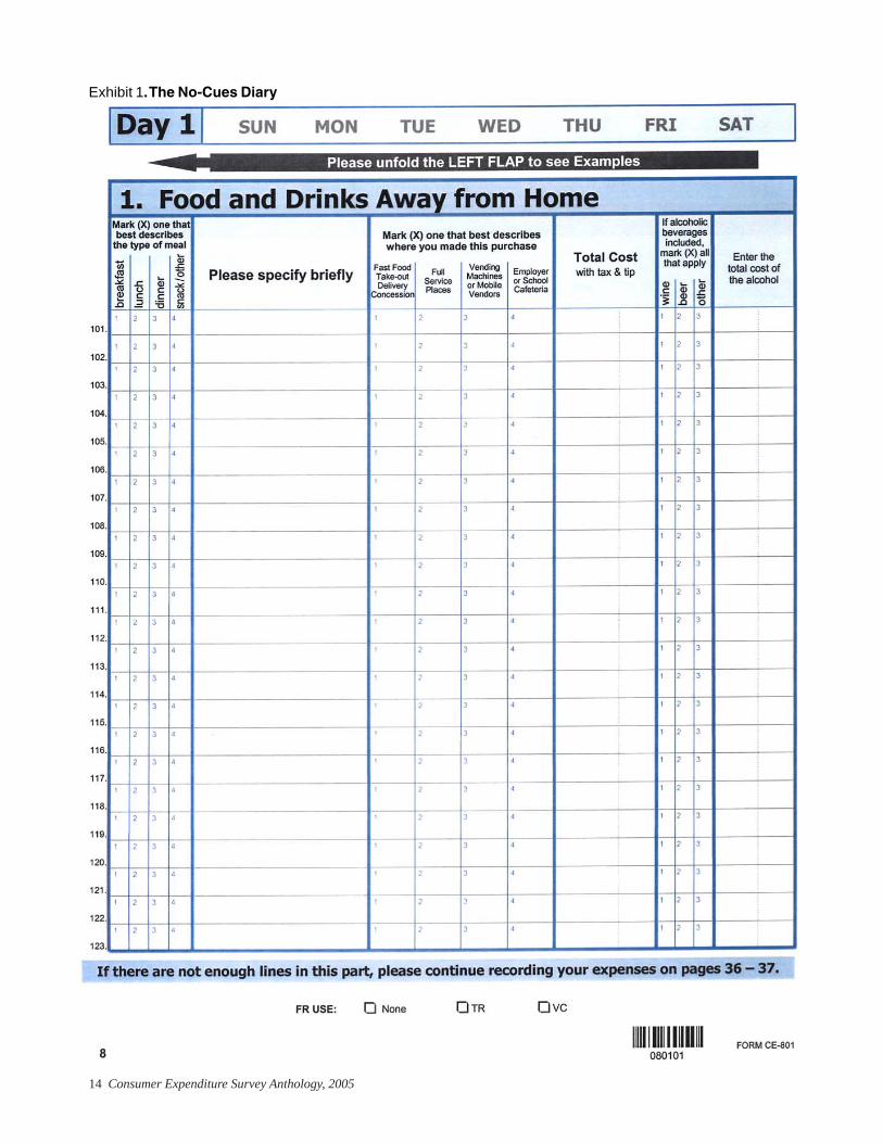
1. The No-Cues Diary. This diarywas similar to the one used inthe 2002 field test and had no cueson the recording pages. (See ex-hibit 1.)
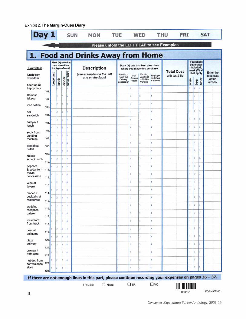
2. The Margin-Cues Diary. Thisdiary listed cues along the leftside of the recording pages. (Seeexhibit 2.)
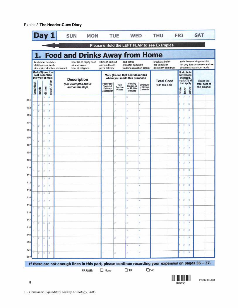
3. The Header-Cues Diary. Thisdiary listed cues along the topof the recording pages. (See ex-hibit 3.)
Selection of cues: Because space onthe recording pages was limited, thenumber of cues had to be minimal, mak-ing the selection of cues an importanttask. The cues were selected on thebasis of four criteria:
1. Analysis of the 2002 field-test data.A comparison was made betweenthe mean expenditures of the Rede-signed Diary and the Current Diary.Because research has shown thatcues improve the reporting of anitem, items for which reported ex-penditures were significantly lowerin the Redesigned Diary comparedwith the Current Diary were identi-fied, and a subset of those items wasselected as cues. Examples includewhite bread, oranges, and wholechicken.
2. Items commonly reported withoutadequate detail. Certain items arecommonly entered into the CEDwith insufficient detail, requiringdata adjustment. For example, en-tries of “gas” must be allocated toeither gasoline or utility gas. Simi-larly, entries of “books” must be al-located to either schoolbooks orother books. To encourage morespecific reporting of items, cuessuch as “gasoline,” “utility gas bill,”“textbooks,” and “cookbook” wereselected.
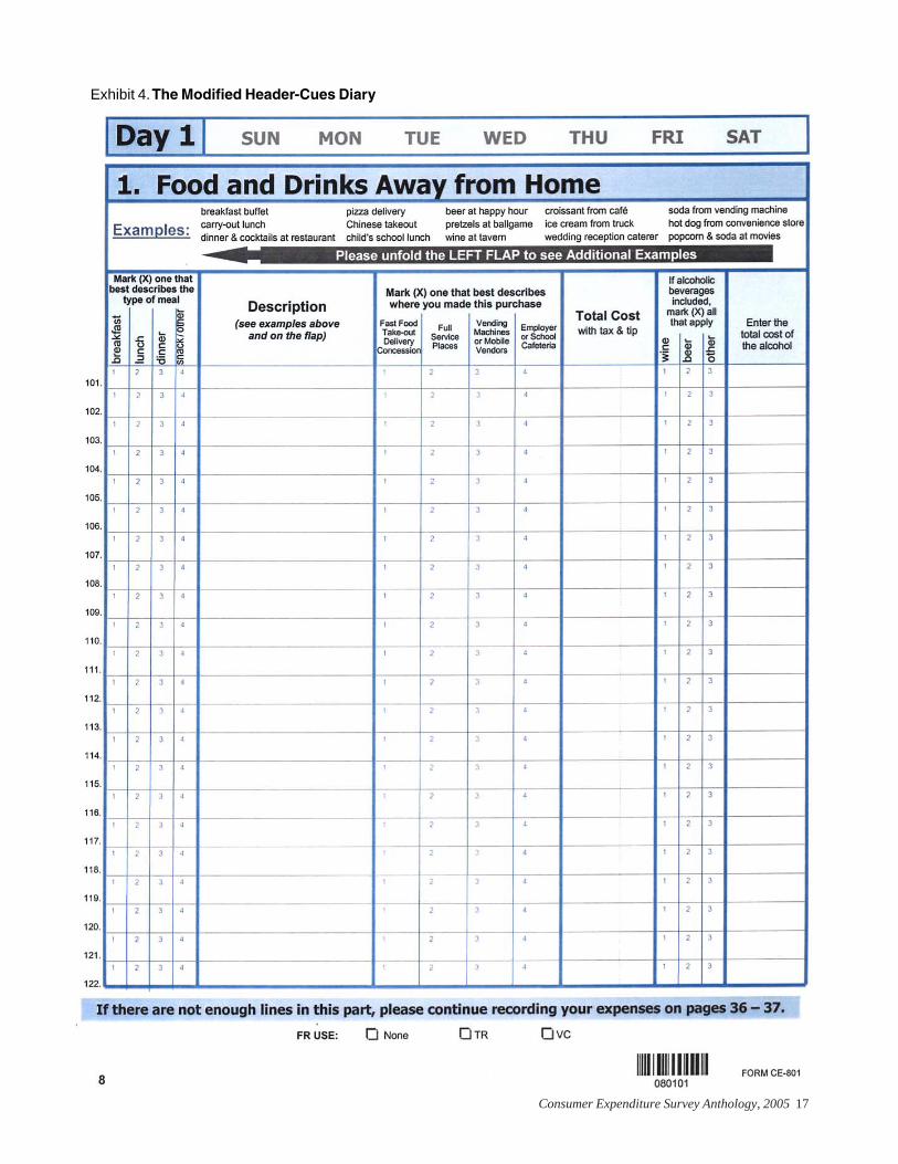
3. Problems identified in the two foodcategories “Food and Drinks Awayfrom Home” and “Food and Drinksfor Home Consumption.”
• Drinks without a meal. Teammembers were concerned thatlinking “Food and Drinks” to-gether in the titles would dis-courage the reporting of drinkswithout a meal. To encouragesuch entries, cues such as “beerat happy hour” and “soda fromvending machine” were selected.
3 Vitrano, F.A., et al., “Cognitive Issuesand Reporting Level Patterns from the CEDiary Operational Test,” in Proceedings ofthe Section on Survey Research Methods.Washington DC: American Statistical Asso-ciation, pp. 262–267, 1988.
4 Roediger, H. L., “Inhibiting Effects ofRecall,” Memory and Cognition, pp. 261–269, 1974.
5 BLS contracts with the U.S. Census Bu-reau to implement the Consumer Expendi-ture Diary Survey in the field.
6 Davis, J., et al., “What Does It ReallyMean to Be User-Friendly when Designingan Expenditure Diary?” paper presented atthe annual meeting of the American Associa-tion of Public Opinion Research (2002). Seealso Davis, J., et al. “Creating a User-FriendlyExpenditure Diary,” Consumer ExpenditureSurvey Anthology, Report 967, pp. 3–17,Sept. 2003.
7 Figueroa, E., et al., “Is a User-FriendlyDiary More Effective? Findings from a FieldTest,” paper presented at the annual meetingof the American Statistical Association, 2003.Although allocations are often used to ac-count for item nonresponse, in the diary theterm refers to an expenditure that does notidentify individual items at the required levelof detail (e.g., a respondent reports “grocer-ies, $150,” rather than the specific itemspurchased). This type of entry requires addi-tional processing to assign the aggregate ex-penditure to target items.
Consumer Expenditure Survey Anthology, 2005 11
• Delivery and takeout meals. Dueto the wording of these two foodentries, the reporting of itemssuch as pizza delivery and Chi-nese takeout is confusing to re-spondents. Both entries shouldbe reported as “Food Away fromHome,” but are often entered as“Food for Home Consumption,”because respondents usuallyconsume these foods in thehome. To encourage enteringthese items in the correct section,cues of “pizza delivery,” “Chi-nese takeout,” and “carryoutlunch” were placed on the “FoodAway from Home” recordingpages.
4. A balanced representation of items.One specific cue from each subcat-egory in the Current Diary was se-lected:
• “cigarettes” from “Tobacco andSmoking Supplies”
• “prescription drugs” from“Medicines, Medical Supplies,and Services”
An effort was made to emphasizeitems that are currently known to beunderreported.
Specificity of the cues: Cues were re-stricted to specific items (e.g., skim milk)that do not require allocation becausethey contain sufficient detail. Cues foritems requiring allocation (e.g., milk)were excluded from consideration. Itwas thought that cuing for sufficientdetail would instruct respondents torecord expenditures with similar speci-ficity. A BLS study of the CED in theearly 1990s noted that cued items havehigher reporting rates when the cuesare specific (e.g., chuck roast vs. beef).8
Order of the cues: Most cues aregrouped with similar items (e.g., wine,beer, and liquor) to emphasize the vari-ety and specificity desired. Pairs of
cues selected to encourage more spe-cific reporting of items were placed nextto one another to illustrate the impor-tance of distinguishing similar items(e.g., “gasoline” and “utility gas bill”were placed next to each other to avoidan entry such as “gas”).
B. ParticipantsParticipants for this study were re-cruited from a database maintained bythe BLS Office of Survey Methods Re-search and through an advertisementplaced in a local newspaper. Sixty-oneindividuals were recruited throughthese methods, together with an addi-tional 5 BLS employees, for a total of66 participants, all from the Washing-ton, DC, area. Thirty-four participantswere women, and while no informationon race or ethnicity was collected,observationally, there appeared to be abalance among African-Americans,Caucasians, and Hispanics. The aver-age age of the participants was 42, withsubjects ranging from 17 to 77 years.The completed education level of theparticipants ranged from 11th grade todoctorate. The average education levelof the participants was 16 years,equivalent to a college degree. Aboutone-third of the participants (n = 24)were employed part time, one-third(n=19) full time, and the remaining par-ticipants were unemployed (n = 9), self-employed (n = 6), and retired (n = 3).The average self-reported income was$37,000. The median income was$31,000, with reports ranging from $800to $100,000.
Twenty-four participants weresingle, 19 were married, 13 were di-vorced, and 3 were widowed. Of thosefrom whom data were collected, half hadchildren (n = 28) and half did not. Themedian number of children per partici-pant was one, and the ages of the chil-dren ranged from 1 to 42 years, withthe average being 22 years.
C. Study design
1. The recall task. Each participantwas provided a diary and asked toenter all of his or her household’sexpenses for the previous week.Since respondents in the field would
be able to use receipts, checkbooks,and other records to help them com-plete the diary, any participant whohad such records available was al-lowed to use them. Diaries were dis-tributed among three groups of parti-ticipants, with 21 participants receiv-ing the No-Cues Diary, 23 receivingthe Margin-Cues Diary, and 20 re-ceiving the Header-Cues Diary.9
2. The recognition task. After com-pleting the diary-recall task, partici-pants were given a comprehensivelist of commonly purchased and fre-quently forgotten items and wereasked to check off all items, includ-ing those they had recorded in thediary, that they or anyone in theirhousehold had purchased duringthe past week.
Recall versus recognition.. Researchon memory has revealed that, whengiven a recall task and a recognitiontask, participants are able to remembermore items with the recognition task10
(Standing et al., 1970, and Sternberg,1999). Therefore, it was thought thatparticipants in this study would iden-tify more of the purchases made bytheir households when using the rec-ognition list than had been reported bycompleting the diary (a pure recall task).The items that were checked on the rec-ognition list, but not recorded in thediary during the recall task, would pro-vide some measure of underreporting(how many items respondents forgotwhen completing the pure recall taskof recording in the diary).
Results from the study showed thatthe average number of unique recogni-tion items reported by participants wasgreater than the average number ofunique diary (or recall) items reported.There was no significant difference
8 Dippo, C.S., and Norwood, J.L., “A Re-view of Research at the Bureau of Labor Sta-tistics,” in Questions about Questions, ed.J.M. Tanur: Russell Sage Foundation, NY, pp.271–290, 1992.
9 The original sample contained 66 dia-ries. Due to data problems, 2 diaries from thegroup receiving the Header-Cues Diary wereeliminated from the analysis.
10 Standing, L., et al., “Perception andmemory for pictures: Single-trial learning of2500 visual stimuli,” Psychonomic Science,19, pp. 73–74, 1970. Also Sternberg, R.J.,Cognitive Psychology, 2nd edition. HarcourtBrace College Publishers, New York, 1999.
12 Consumer Expenditure Survey Anthology, 2005
(ANOVA) was performed to test differ-ences between the three diary formson the following factors:11
• Overall level of expenditures
• Total number of items reported
• Number of unique diary items(items recorded only with the re-call task)
• Number of unique recognitionitems (items checked only withthe recognition task)
• Percent of reported items requir-ing allocation
• Percent of items that matched thecues verbatim
Comparing diary items
The only significant difference foundamong the three types of diaries wasthe average proportion of items match-ing the cues printed on the recordingpages verbatim. (See table 1.) Comparedwith the No-Cues diary, the Margin-Cues Diary and the Header-Cues Diaryboth had more than twice the propor-tion of items matching the cues (7 per-cent, as opposed to 19 and 20 percent,respectively). This difference suggeststhat the participants were looking at thecues on the pages. However, there wasno significant difference between theMargin-Cues Diary and the Header-Cues Diary (19.1 percent and 19.7 per-cent, respectively).
No significant differences werefound on any of the other variablesmeasured, including number of uniquediary items recalled, number of uniquerecognition items reported, and per-centage of items requiring allocationdue to inadequate detail in reporting.
Comparing diary expenditures
No significant differences in expendi-tures were found among the three dia-ries.
across the diaries in the percentage ofrespondents underreporting. (See table1.)
3. Followup questionnaire and debrief-ing. After completing both the recalland recognition tasks, participantswere given a questionnaire about theirexperience with the diary. There was aseparate questionnaire for each diaryformat. The questions were designedto identify the various features of thecues, including the location, format,and the actual cues that were selected.
Finally, before concluding the ses-sion, each participant received a 5-minute debriefing in which he or shehad the opportunity to provide furthercomments.
Findings
A. Qualitative findings
Observational findings
Because the goal of the study was toexamine the impact of adding cues tothe recording pages of the RedesignedDiary, it was important to identify anyproblems participants had that ap-peared to be a direct result of the cues.This goal was achieved by observingthe participants and noting the ques-tions they asked as they completed thetasks and then reviewing each diary forerrors.
One of the main problems found waswith the Margin-Cues Diary. A few par-ticipants circled the margin cues in-stead of entering the description in thespace provided. This problem mayhave stemmed from the visual layoutof the vertically formatted cues in theMargin-Cues Diary, compared with thehorizontally formatted cues in theHeader-Cues Diary. Apparently, whencues are listed vertically, some partici-pants are more likely to view them as acomprehensive list of expenses to circlethan when they are listed horizontally.
When recalling their purchases,some participants asked what theyshould do if they didn’t buy somethingthat was listed. Others asked what theyshould do if they purchased somethingthat was not listed. These questions
suggested that some participants didnot fully understand the purpose of thecues and thought of them as compre-hensive lists from which they had tochoose. This type of confusion couldlead to overreporting of cued items andunderreporting of noncued items.
Findings from the followup question-naire
Because the cues were designed to helpparticipants recall items they may havepurchased, one question askedwhether the participants used thesample items (on the flap of the No-Cues Diary, listed along the side of therecording pages in the Margin-CuesDiary, and listed along the top of therecording page in the Header-Cues Di-ary) to help them remember their pur-chases. Among participants using theNo-Cues Diary, 50 percent reported thatthey found the sample items helpful inremembering purchases. Almost 70 per-cent of participants using the Margin-Cues Diary said the cues along the sideof the recording pages were helpful,and 86 percent of respondents usingthe Header-Cues Diary reported thatthe sample cues along the top of therecording pages were helpful.
In addition, the majority of the par-ticipants indicated that cues were help-ful for determining which purchases torecord, how to record purchases, andin which section to record purchases.
Findings from the debriefing
The debriefing questions provided ad-ditional feedback about the partici-pants’ experience with the diary, so anycomments they made regarding thecues were seen as particularly useful.Many participants stated that the ex-amples were very helpful. Although theterm “examples” may have been usedto denote examples anywhere in thediary, some participants specificallyreferred to the cues listed along the topof the page or cues along the side ofthe recording page.
B. Quantitative findingsA one-way analysis of variance
11 Where the data met the assumptionsrequired for ANOVA. When the data violatedthese assumptions, the nonparametricWilcoxon Rank Sum test was performed.
Consumer Expenditure Survey Anthology, 2005 13
more extensive list.
The Modified Header-Cues Diary(exhibit 4) will be implemented in Janu-ary 2005.
In 1980, the CED had five broad cat-egories, which were then divided into42 detailed subcategories in 1991. In2005, the subcategories will be re-moved, leaving four broad categories.In terms of the specific cues it con-tains, the CED went from 76 in 1980 to305 in 1991. The 2005 diary has 89 spe-cific cues.
Will the combination of a user-friendly layout and a decreased num-ber of specific cues on the recordingpages have a positive impact on re-sponse rates and quality of the data?Did BLS strike the right balance be-tween too many cues and too few?These questions will be answered af-ter data are collected with the Rede-signed Diary in 2005.
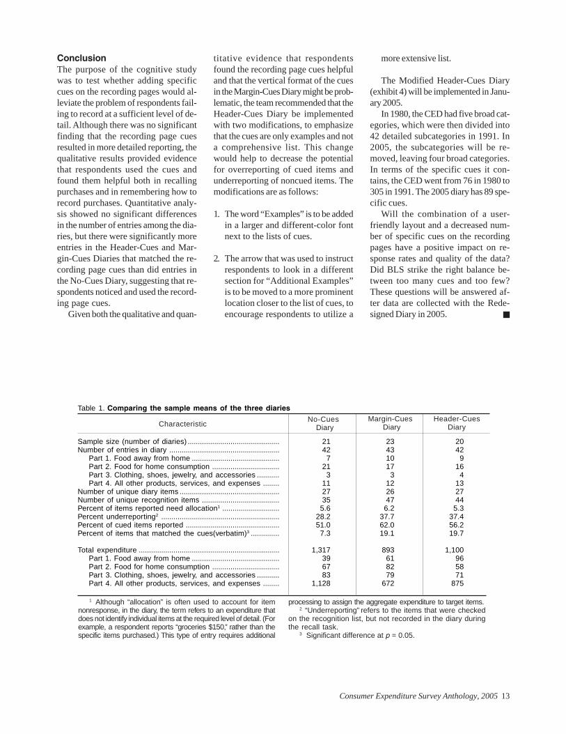
ConclusionThe purpose of the cognitive studywas to test whether adding specificcues on the recording pages would al-leviate the problem of respondents fail-ing to record at a sufficient level of de-tail. Although there was no significantfinding that the recording page cuesresulted in more detailed reporting, thequalitative results provided evidencethat respondents used the cues andfound them helpful both in recallingpurchases and in remembering how torecord purchases. Quantitative analy-sis showed no significant differencesin the number of entries among the dia-ries, but there were significantly moreentries in the Header-Cues and Mar-gin-Cues Diaries that matched the re-cording page cues than did entries inthe No-Cues Diary, suggesting that re-spondents noticed and used the record-ing page cues.
Given both the qualitative and quan-
titative evidence that respondentsfound the recording page cues helpfuland that the vertical format of the cuesin the Margin-Cues Diary might be prob-lematic, the team recommended that theHeader-Cues Diary be implementedwith two modifications, to emphasizethat the cues are only examples and nota comprehensive list. This changewould help to decrease the potentialfor overreporting of cued items andunderreporting of noncued items. Themodifications are as follows:
1. The word “Examples” is to be addedin a larger and different-color fontnext to the lists of cues.
2. The arrow that was used to instructrespondents to look in a differentsection for “Additional Examples”is to be moved to a more prominentlocation closer to the list of cues, toencourage respondents to utilize a
Table 1. Comparing the sample means of the three diaries
Sample size (number of diaries) ............................................. 21 23 20Number of entries in diary ...................................................... 42 43 42
Part 1. Food away from home ........................................... 7 10 9Part 2. Food for home consumption ................................. 21 17 16Part 3. Clothing, shoes, jewelry, and accessories ........... 3 3 4Part 4. All other products, services, and expenses ........ 11 12 13
Number of unique diary items ................................................. 27 26 27Number of unique recognition items ...................................... 35 47 44Percent of items reported need allocation1 ............................ 5.6 6.2 5.3Percent underreporting2 .......................................................... 28.2 37.7 37.4Percent of cued items reported .............................................. 51.0 62.0 56.2Percent of items that matched the cues(verbatim)3 .............. 7.3 19.1 19.7
Total expenditure ..................................................................... 1,317 893 1,100Part 1. Food away from home ........................................... 39 61 96Part 2. Food for home consumption ................................. 67 82 58Part 3. Clothing, shoes, jewelry, and accessories ........... 83 79 71Part 4. All other products, services, and expenses ........ 1,128 672 875
Header-CuesDiary
Margin-Cues Diary
No-Cues Diary
1 Although “allocation” is often used to account for itemnonresponse, in the diary, the term refers to an expenditure thatdoes not identify individual items at the required level of detail. (Forexample, a respondent reports “groceries $150,” rather than thespecific items purchased.) This type of entry requires additional
processing to assign the aggregate expenditure to target items.2 “Underreporting” refers to the items that were checked
on the recognition list, but not recorded in the diary duringthe recall task.
3 Significant difference at p = 0.05.
Characteristic
14 Consumer Expenditure Survey Anthology, 2005
Exhibit 1. The No-Cues Diary
Consumer Expenditure Survey Anthology, 2005 15
Exhibit 2. The Margin-Cues Diary
16 Consumer Expenditure Survey Anthology, 2005
Exhibit 3.The Header-Cues Diary
Consumer Expenditure Survey Anthology, 2005 17
Exhibit 4. The Modified Header-Cues Diary
18 Consumer Expenditure Survey Anthology, 2005
The Consumer Expenditure Quar-terly Interview Survey collectsdata from selected consumer
units (CUs) across the United States.Participating CUs are interviewed fivetimes, and their responses from the sec-ond through fifth interviews providedata that are used in publications. SomeCUs complete interviews 2 through 5;other CUs complete some, but not all,of these interviews; and some CUs donot complete any interviews. TheseCUs are called complete responders,intermittent responders, and nonre-sponders, respectively.
A study describing differences indemographic characteristics betweencomplete and intermittent responders,and estimating the effect of nonre-sponses from intermittent responders onpublished consumer expenditure esti-mates, appeared in a previous U.S. Bu-reau of Labor Statistics (BLS) publica-tion. (See “Characteristics of Completeand Intermittent Responders in theConsumer Expenditure Quarterly Inter-view Survey” by Sally E. Reyes-Mo-rales, Consumer Expenditure SurveyAnthology, 2003, Report 967, Sept.2003.) This article presents results of astudy of the characteristics ofnonresponder CUs, who were excludedfrom the aforementioned study.
Background and definitionsThe U.S. Census Bureau conducts theConsumer Expenditure Survey for BLS
Characteristics ofNonresponders in theConsumer ExpenditureQuarterly InterviewSurvey
Sally E. Reyes-Morales is a mathematical stat-istician in the Division of Price StatisticalMethods, Branch of Consumer ExpenditureSurveys, Bureau of Labor Statistics.
to find out how Americans spend theirmoney. Census Bureau field represen-tatives collect data from a randomsample of CUs chosen through sys-tematic sampling of residential ad-dresses across the United States. Thissample is representative of the totalU.S. civilian population not living ininstitutions.
The Consumer Expenditure Quar-terly Interview Survey is a rotatingpanel survey. CUs are interviewed onceper quarter for five consecutive quar-ters. After the fifth quarter, CUs leavethe sample and are replaced by new CUsselected as before through systematicsampling of residential addresses.
In the initial interview, field repre-sentatives ask respondents to reportall expenditures they made during theprevious month. This interview is usedonly for “bounding” purposes—thatis, to make sure the expenditures re-ported in the second through fifth in-terviews reflect the correct periods. Inthe second through fifth interviews,field representatives collect data for the3 months prior to the interview. Onlythe expenditure data collected in thesecond through fifth interviews areused to compute official consumer ex-penditure estimates. Because data col-lected in each quarter are treated inde-pendently, annual estimates do notdepend on CUs participating for all fivequarters.
Terms used in this document are de-
SALLY E. REYES-MORALES
Consumer Expenditure Survey Anthology, 2005 19
fined below:Household. The people who occupy ahousing unit. A housing unit is ahouse, an apartment, a mobile home, aroom, or a group of rooms occupied (orintended to be occupied) as separateliving quarters.
Consumer unit (CU). Members of ahousehold related by blood, marriage,adoption, or some other legal arrange-ment; a single person living alone orsharing a household with others butwho is financially independent; or twoor more persons living together whoshare responsibility for at least two ofthe three major types of expenses:Food, housing, and other expenses.Students living in university housingare also included in the sample as sepa-rate consumer units.
Respondent. Ideally an adult house-hold member who is familiar with all ofthe expenditures that his/her CUmakes. An eligible respondent is anyhousehold member who is age 16 orolder and who can answer questionson household and consumer unit com-position accurately.
INSTAT. Interview status (ranges from01 to 19):
01 = Interview
Type A noninterview:02 = No one home03 = Temporarily absent04 = Refused05 = Other Type A noninterview
Type B noninterview:06 = Vacant (for rent)07 = Vacant (for sale)08 = Vacant (other)09 = Occupied by person whose usual
residence is elsewhere10 = Under construction (not ready)11 = Other Type B noninterview
Type C noninterview:12 = Demolished13 = House or mobile home moved14 = Converted to nonresidential use15 = Merged16 = Condemned17 = Located on military base18 = CU moved19 = Other Type C noninterview
Interview. Completed by an eligible CU
(INSTAT = 01).
Type A noninterview. Occurs when anaddress is within the scope of the sur-vey and eligible for interview, but aninterview is not obtained (INSTAT =02 through 05).
Type B noninterview. Occurs when anaddress is within the scope of the sur-vey but is not eligible for interview(INSTAT = 06 through 11).
Type C noninterview. Occurs when anaddress is out of the scope of the sur-vey or is permanently ineligible for thesurvey sample (INSTAT = 12 through19).
Record. Contains all the informationrelevant to each interview ornoninterview. Each CU could have asmany as five records.
Nonresponder CUs. CUs who did notcomplete interviews 2 through 5.
Eligible CUs. Nonresponder CUs as-signed a Type A noninterview code inat least one of the last four records.
Ineligible CUs. Nonresponder CUswho had no Type A noninterview codein the last four records.
In-range CUs. CUs who were sched-uled to participate in all five interviewsbetween January 1997 and December2000.
Out-of-range CUs. All CUs who werenot in range.
Consumer units studiedCharacteristics of nonresponder CUsare the focus of this study. Data weredrawn from the universe of ConsumerExpenditure Quarterly Interview Surveyresponder and nonresponder CUs(1997 through 2000) using the follow-ing criteria:
• Only in-range CUs were used,in order to track their historythroughout the survey.
• Only nonresponder CUs wereused in the study.
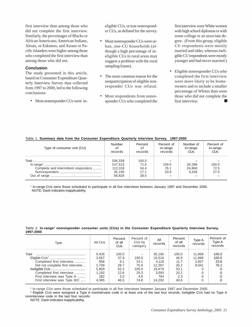
A summary of the 4 years of dataappears in table 1. Because CUs couldparticipate in the survey for five quar-ters, they could have as many as fiverecords. Of the total number of CUrecords in the sample during the pe-riod of analysis, 71.5 percent (147,513records) were in range; 28.5 percentwere out of range. Of the in-rangerecords, however, 76.1 percent wereprovided by complete and intermittentresponders, who were excluded fromthe study.
Nonresponder CUs’ records madeup 17.1 percent of all records and 23.9percent of in-range records (corre-sponding to 27.5 percent of in-rangeCUs). Nonresponder CUs were sepa-rated into those who were eligible andthose who were ineligible for interview(table 2). Eligible nonresponder CUswere those assigned a Type Anoninterview code for at least one ofthe last four interviews (interviews 2through 5)—that is, those nonre-sponders who were eligible for inter-view during a particular survey quarterbut did not participate in the surveyfor that period. Conversely, the non-responder CUs categorized as ineligiblewere those CUs coded as Type B non-interviews (ineligible for interview be-cause the residence was vacant, occu-pied by temporary residents, or underconstruction) or Type C nonin-terviews (out of the scope of the sur-vey because the residence was demol-ished, abandoned, or converted tononresidential use) for each of the lastfour interviews.
Most nonresponder CUs (62.2 per-cent) were categorized as ineligible forinterview. The remaining 37.8 percentwere eligible for interview at some pointduring the last four quarters of the sur-vey but did not complete interviews.Accordingly, ineligible nonresponderCUs made up a larger percentage (53.1percent) of records than did eligiblenonresponder CUs (46.9 percent).
Although nonresponder CUs didnot complete any of the last four inter-views, some of them completed the first(bounding) interview. Nonresponder
20 Consumer Expenditure Survey Anthology, 2005
CUs who completed the first interviewaccounted for 21.7 percent of all CUsin the study (9.1 percent of eligible CUsand 12.6 percent of ineligible CUs).
Of the ineligible nonresponder CUs,74.8 percent were coded as Type B orType C noninterview at the initial inter-view. This shows that most ineligiblenonresponder CUs were true nonre-sponders, as defined for the survey:they were ineligible for interview anddid not contribute to the survey’s re-sponse rate. The remaining 25.1 per-cent can be divided into those that com-pleted the first interview (20.3 percent)and those for whom the first interviewresulted in a Type A noninterview (4.8percent).
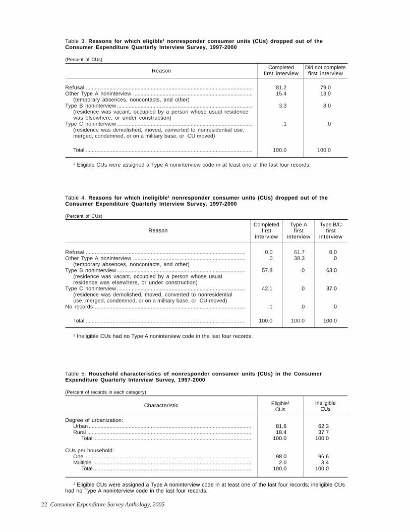
Reasons for dropping out of thesurveyReasons for which CUs dropped outof the survey can be identified by theinterview code of the first noninterview.
Table 3 shows that, among eligiblenonresponder CUs, refusal was themost common reason for nonparti-cipation, accounting for 81.2 percentof nonresponder CUs who completedthe first interview and 79.0 percent ofthose who did not complete the firstinterview. (Four out of five instancesof nonparticipation in the survey weredue to the refusal of the CU respon-dent.) The second most common rea-son was an “Other Type A noninter-view,” accounting for 15.4 percent ofthose who did and 13.0 percent of thosewho did not complete the first inter-view. Because the rankings of the rea-sons for nonparticipation and their re-spective percentages were similar forboth categories, completion or non-completion of the first interview seemsto have factored little in a CU droppingout of the survey.
Ineligible nonresponders can bepartitioned into three distinct groups.(See table 4.) The first group comprisesCUs who participated in the first inter-view but became ineligible for subse-quent interviews. In this group thereare more CUs coded Type Bnoninterview (57.8 percent) than TypeC noninterview (42.1 percent).
CUs who were coded as a Type A
noninterview for the first interview andbecame ineligible for subsequent inter-views constitute the second group. Forthese CUs, the leading reason for notparticipating in the survey (61.7 per-cent of the responses) was refusal; theother reasons were combined into“Other Type A noninterview” (38.3percent).
The last group of ineligible CUs in-cluded those who did not complete anyof the five interviews and for whichnone of the noninterviews were codedas Type A. For these CUs, the bound-ing interview was coded as a Type Bnoninterview (ineligible; 63.0 percent)or as a Type C noninterview (out ofscope; 37.0 percent).
There were no conversions to TypeA noninterview in any of the four sub-sequent interviews for any of the threegroups of ineligible CUs.
Household and respondent char-acteristicsThe demographic characteristics of thenonresponders at the household andCU levels are summarized in tables 5, 6,and 7. Household tenure, race, andmean family size cannot be obtainedfor ineligible CUs, but degree of urban-ization (urban or rural) and CUs perhousehold (one or multiple) are pre-sented in table 5 from all five interviewsfor eligible and ineligible CUs. Percent-ages of rural CUs and multiple-CUhouseholds are larger for ineligible CUsthan for eligible CUs (37.7 percent and3.4 percent compared with 18.4 percentand 2.0 percent, respectively). The rela-tively high percentage of rural house-holds in the ineligible column may sug-gest a problem with the rural samplingframe (the list of all addresses in thetarget population from which thesample is selected.) The sampling framemay be more accurate in urban areas;the rural sampling frame may containaddresses that are out of the scope ofthis survey.
Comparative statistics about thedemographic characteristics of thenonresponder CUs at the householdand consumer-unit levels are given intables 6 and 7.
Table 6 presents the race, sex, mari-
tal status, age range, and education ofrespondents from eligible and ineligibleCUs who completed the first interview.Respondents from eligible nonre-sponder CUs who completed the firstinterview tended to be White (78.9 per-cent) women (59.1 percent) who weremarried (43.1 percent), were 65 or older(16.8 percent), and had at most a highschool diploma (28.8 percent). Respon-dents from ineligible nonresponder CUswho completed the first interview weremostly White (80.6 percent) women (53.9percent) who had never married (41.9percent), were under 25 years old (24.1percent), and had at most some collegeor an associate degree (36.6 percent).
Both eligible and ineligible nonre-sponder CUs had high percentages ofwhite female respondents. Eligible CUshad a higher percentage of married re-spondents than of any other category,while ineligible CUs had a higher per-centage of those who never marriedthan of any other category. EligibleCUs had a higher percentage of respon-dents aged 65 and older, and ineligibleCUs a higher percentage of respon-dents under age 25. Eligible CUs had alarger percentage of respondentswhose highest educational level washigh school, whereas ineligible CUs hada larger percentage of respondents withsome college or associate degree.
Table 7 gives summary statisticsabout characteristics of eligiblenonresponder CUs who had Type Anoninterviews. Eligible CUs are sepa-rated into two groups, those who com-pleted the first interview and those whodid not. Mean family size was slightlygreater (2.4) for CUs who completed thefirst interview than for those who didnot (2.2). Percentages of urban CUsand one-CU households differed littlebetween CUs who completed the firstinterview and those who did not—78.2percent and 97.5 percent compared with81.9 percent and 98.6 percent, respec-tively.
There appears to be a relationshipbetween household tenure and raceand whether an eligible nonresponderCU completed the first interview. Thepercentage of homeowners was high-er among those who completed the
Consumer Expenditure Survey Anthology, 2005 21
first interview than among those whodid not complete the first interview.Similarly, the percentages of Blacks orAfrican Americans; American Indians,Aleuts, or Eskimos; and Asians or Pa-cific Islanders were higher among thosewho completed the first interview thanamong those who did not.
ConclusionThe study presented in this article,based on Consumer Expenditure Quar-terly Interview Survey data collectedfrom 1997 to 2000, led to the followingconclusions:
• Most nonresponder CUs were in-
eligible CUs, or true nonrespond-er CUs, as defined for the survey.
• Most nonresponder CUs were ur-ban, one-CU households (al-though a high percentage of in-eligible CUs in rural areas maysuggest a problem with the ruralsampling frame).
• The most common reason for thenonparticipation of eligible non-responder CUs was refusal.
• Most respondents from nonre-sponder CUs who completed the
first interview were White womenwith high school diplomas or withsome college or an associate de-gree. (From this group, eligibleCU respondents were mostlymarried and older, whereas ineli-gible CU respondents were mostlyyounger and had never married.)
• Eligible nonresponder CUs whocompleted the first interviewwere more likely to be home-owners and to include a smallerpercentage of Whites than werethose who did not complete thefirst interview.
Table 1. Summary data from the Consumer Expenditure Quarterly Interview Survey, 1997-2000
Total ............................................................................ 206,339 100.0 – – –In range1 ............................................................... 147,513 71.5 100.0 34,286 100.0
Complete and intermittent responders .......... 112,318 54.4 76.1 24,860 72.5Nonresponders .............................................. 35,195 17.1 23.9 9,426 27.5
Out of range ........................................................ 58,826 28.5 – – –
1 In-range CUs were those scheduled to participate in all five interviews between January 1997 and December 2000.NOTE: Dash indicates inapplicability.
Numberof
records
Percentof
records
Percent ofin-rangerecords
Number ofin-range
CUs
Percent ofin-range
CUsType of consumer unit (CU)
Table 2. In-range1 nonresponder consumer units (CUs) in the Consumer Expenditure Quarterly Interview Survey,1997-2000
Total ...................................................... 9,426 100.0 – 35,195 100.0 11,868 100.0Eligible CUs ........................................ 3,567 37.8 100.0 16,516 46.9 11,868 100.0
Completed first interview ............ 858 9.1 24.1 4,119 11.7 2,827 23.8Did not complete first interview .. 2,709 28.7 75.9 12,397 35.2 9,041 76.2
Ineligible CUs ...................................... 5,859 62.2 100.0 18,679 53.1 0 .0Completed first interview ............ 1,192 12.6 20.3 3,593 10.2 0 .0First interview was Type A ......... 282 3.0 4.8 794 2.3 0 .0First interview was Type B/C ..... 4,385 46.5 74.8 14,292 40.6 0 .0
All CUsPercent
of allCUs
Percent ofCUs by
category
Allrecords
Percentof all
records
Type Arecords
Percent ofType A
recordsType
1 In-range CUs were those scheduled to participate in all five interviews between January 1997 and December 2000.2 Eligible CUs were assigned a Type A noninterview code in at least one of the last four records; ineligible CUs had no Type A
noninterview code in the last four records.NOTE: Dash indicates inapplicability.
2
22 Consumer Expenditure Survey Anthology, 2005
Table 4. Reasons for which ineligible1 nonresponder consumer units (CUs) dropped out of theConsumer Expenditure Quarterly Interview Survey, 1997-2000
(Percent of CUs)
Refusal ............................................................................................................ 0.0 61.7 0.0Other Type A noninterview ............................................................................ .0 38.3 .0
(temporary absences, noncontacts, and other)Type B noninterview ....................................................................................... 57.8 .0 63.0
(residence was vacant, occupied by a person whose usualresidence was elsewhere, or under construction)
Type C noninterview ....................................................................................... 42.1 .0 37.0(residence was demolished, moved, converted to nonresidentialuse, merged, condemned, or on a military base, or CU moved)
No records ...................................................................................................... .1 .0 .0
Total ............................................................................................................ 100.0 100.0 100.0
Type B/Cfirst
interview
Completedfirst
interview
Type Afirst
interviewReason
1 Ineligible CUs had no Type A noninterview code in the last four records.
Table 5. Household characteristics of nonresponder consumer units (CUs) in the ConsumerExpenditure Quarterly Interview Survey, 1997-2000
(Percent of records in each category)
Degree of urbanization:Urban .............................................................................................................. 81.6 62.3Rural ............................................................................................................... 18.4 37.7
Total ........................................................................................................... 100.0 100.0
CUs per household:One ................................................................................................................. 98.0 96.6Multiple ........................................................................................................... 2.0 3.4
Total ........................................................................................................... 100.0 100.0
Characteristic Eligible1
CUsIneligible
CUs
1 Eligible CUs were assigned a Type A noninterview code in at least one of the last four records; ineligible CUshad no Type A noninterview code in the last four records.
Table 3. Reasons for which eligible1 nonresponder consumer units (CUs) dropped out of theConsumer Expenditure Quarterly Interview Survey, 1997-2000
(Percent of CUs)
Refusal ................................................................................................................. 81.2 79.0Other Type A noninterview ................................................................................. 15.4 13.0
(temporary absences, noncontacts, and other)Type B noninterview ............................................................................................ 3.3 8.0
(residence was vacant, occupied by a person whose usual residencewas elsewhere, or under construction)
Type C noninterview ............................................................................................ .1 .0(residence was demolished, moved, converted to nonresidential use,merged, condemned, or on a military base, or CU moved)
Total ................................................................................................................. 100.0 100.0
Reason Completedfirst interview
Did not completefirst interview
1 Eligible CUs were assigned a Type A noninterview code in at least one of the last four records.
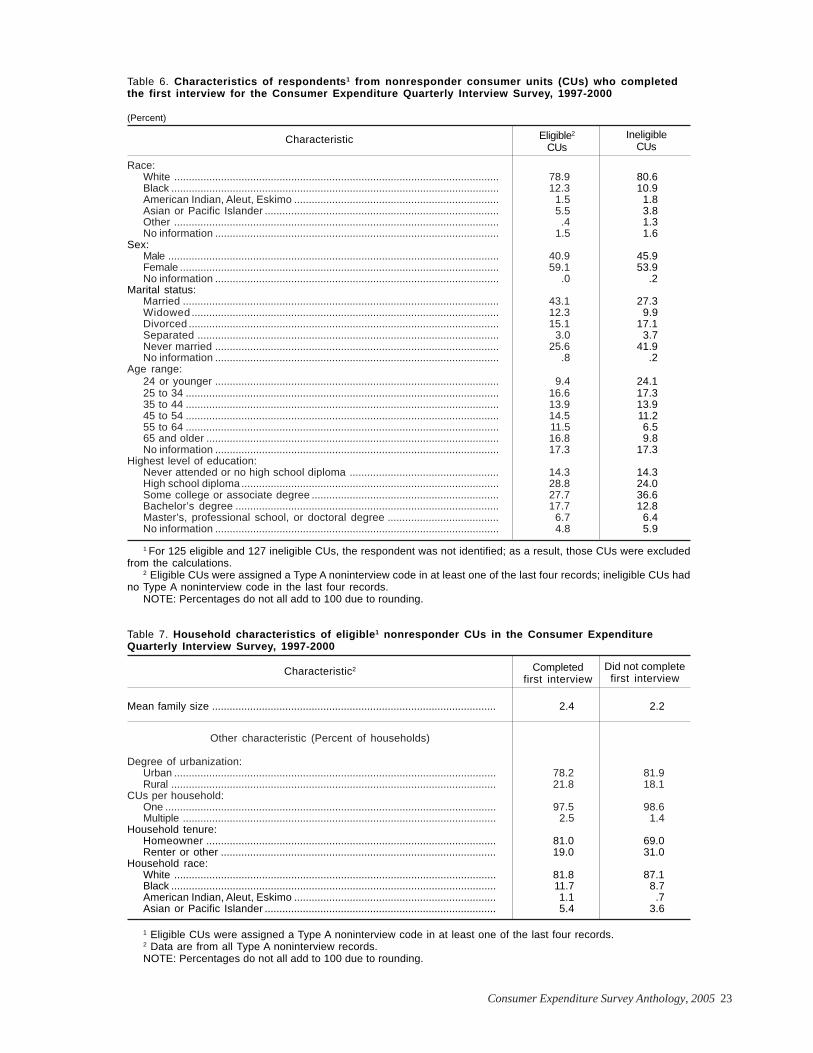
Consumer Expenditure Survey Anthology, 2005 23
1 Eligible CUs were assigned a Type A noninterview code in at least one of the last four records.2 Data are from all Type A noninterview records.NOTE: Percentages do not all add to 100 due to rounding.
Table 7. Household characteristics of eligible1 nonresponder CUs in the Consumer ExpenditureQuarterly Interview Survey, 1997-2000
Mean family size ................................................................................................. 2.4 2.2
Degree of urbanization:Urban .............................................................................................................. 78.2 81.9Rural ............................................................................................................... 21.8 18.1
CUs per household:One ................................................................................................................. 97.5 98.6Multiple ........................................................................................................... 2.5 1.4
Household tenure:Homeowner ................................................................................................... 81.0 69.0Renter or other .............................................................................................. 19.0 31.0
Household race:White .............................................................................................................. 81.8 87.1Black ............................................................................................................... 11.7 8.7American Indian, Aleut, Eskimo ..................................................................... 1.1 .7Asian or Pacific Islander ............................................................................... 5.4 3.6
Characteristic2 Completedfirst interview
Did not completefirst interview
Other characteristic (Percent of households)
Table 6. Characteristics of respondents1 from nonresponder consumer units (CUs) who completedthe first interview for the Consumer Expenditure Quarterly Interview Survey, 1997-2000
(Percent)
Race:White ............................................................................................................... 78.9 80.6Black ................................................................................................................ 12.3 10.9American Indian, Aleut, Eskimo ...................................................................... 1.5 1.8Asian or Pacific Islander ................................................................................ 5.5 3.8Other ............................................................................................................... .4 1.3No information ................................................................................................. 1.5 1.6
Sex:Male ................................................................................................................. 40.9 45.9Female ............................................................................................................. 59.1 53.9No information ................................................................................................. .0 .2
Marital status:Married ............................................................................................................ 43.1 27.3Widowed ......................................................................................................... 12.3 9.9Divorced .......................................................................................................... 15.1 17.1Separated ....................................................................................................... 3.0 3.7Never married ................................................................................................. 25.6 41.9No information ................................................................................................. .8 .2
Age range:24 or younger ................................................................................................. 9.4 24.125 to 34 ........................................................................................................... 16.6 17.335 to 44 ........................................................................................................... 13.9 13.945 to 54 ........................................................................................................... 14.5 11.255 to 64 ........................................................................................................... 11.5 6.565 and older .................................................................................................... 16.8 9.8No information ................................................................................................. 17.3 17.3
Highest level of education:Never attended or no high school diploma ................................................... 14.3 14.3High school diploma ........................................................................................ 28.8 24.0Some college or associate degree ................................................................ 27.7 36.6Bachelor’s degree .......................................................................................... 17.7 12.8Master’s, professional school, or doctoral degree ...................................... 6.7 6.4No information ................................................................................................. 4.8 5.9
Characteristic Eligible2
CUsIneligible
CUs
1 For 125 eligible and 127 ineligible CUs, the respondent was not identified; as a result, those CUs were excludedfrom the calculations.
2 Eligible CUs were assigned a Type A noninterview code in at least one of the last four records; ineligible CUs hadno Type A noninterview code in the last four records.
NOTE: Percentages do not all add to 100 due to rounding.
24 Consumer Expenditure Survey Anthology, 2005
Determining Area SampleSizes for the ConsumerExpenditure Survey
SYLVIA A. JOHNSON-HERRINGSHARON KRIEGERDAVID SWANSON
Sylvia A. Johnson-Herring is a mathematicalstatistician in the Division of Price Statisti-cal Methods, Consumer Expenditure Surveys,Bureau of Labor Statistics.
Sharon Krieger is a mathematical statisticianin the Division of Price Statistical Methods,Consumer Expenditure Surveys, Bureau ofLabor Statistics.
David Swanson is Branch Chief, Division ofPrice Statistical Methods, Consumer Expen-diture Surveys, Bureau of Labor Statistics.
The Consumer Expenditure Sur-vey (CE) is a national house-hold survey conducted by the
U.S. Bureau of Labor Statistics (BLS)to find out how Americans spend theirmoney. The survey’s sample design,based on the decennial census, is up-dated approximately every 10 years. Atthat time, many decisions need to bemade, such as the number of geographicareas in which to collect data and thenumber of households from which tocollect data in each area. This articledescribes a new method for makingthese decisions, one that has been in-corporated in the sample design to beintroduced in 2005.
BackgroundThe CE is used to produce the mostaccurate estimate of consumer expen-ditures possible at the national level.The U.S. Consumer Price Index (CPI)program relies on CE data to produceinflation estimates. The most compre-hensive CPI is based on the expendi-ture patterns of consumers in urbanand metropolitan areas and is denotedCPI-U. The CPI-U population repre-sents about 87 percent of the total U.S.population. The CE is designed to bal-ance the goals of the CE and CPI pro-grams. These goals compete with eachother when BLS allocates the CE’s na-tionwide sample of households to geo-graphic areas covered by the two pro-grams.
The number of households in theCE’s national sample is determined bythe survey’s data collection budget.Allocating this fixed number of house-holds to individual geographic areasmust be done in a way that satisfiesthe competing goals of the CE and CPIprograms as much as possible. The CEprogram’s goal is to allocate the samplehouseholds to the selected geographicareas in proportion to their share of theU.S. population, whereas the CPIprogram’s goal is to allocate samplehouseholds to the selected urban ar-eas in proportion to their share of theNation’s urban population. The CPIprogram further strives to include aminimum number of households in eachselected urban area to ensure the sta-tistical quality of its published priceindexes for those areas.
This article describes a new auto-mated method of allocating the CE’snationwide sample of households in away that balances competing goals andconstraints. The CE actually consistsof two surveys, the Diary and Inter-view surveys, but this article focuseson the Interview survey.
Geographic areas in the CEsampleThe selection of households for thesurvey begins with the definition andselection of primary sampling units(PSUs), which consist of counties (orparts thereof), groups of counties, or
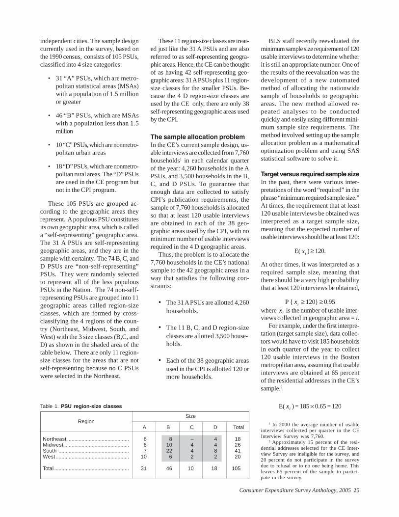
Consumer Expenditure Survey Anthology, 2005 25
independent cities. The sample designcurrently used in the survey, based onthe 1990 census, consists of 105 PSUs,classified into 4 size categories:
• 31 “A” PSUs, which are metro-politan statistical areas (MSAs)with a population of 1.5 millionor greater
• 46 “B” PSUs, which are MSAswith a population less than 1.5million
• 10 “C” PSUs, which are nonmetro-politan urban areas
• 18 “D” PSUs, which are nonmetro-politan rural areas. The “D” PSUsare used in the CE program butnot in the CPI program.
These 105 PSUs are grouped ac-cording to the geographic areas theyrepresent. A populous PSU constitutesits own geographic area, which is calleda “self-representing” geographic area.The 31 A PSUs are self-representinggeographic areas, and they are in thesample with certainty. The 74 B, C, andD PSUs are “non-self-representing”PSUs. They were randomly selectedto represent all of the less populousPSUs in the Nation. The 74 non-self-representing PSUs are grouped into 11geographic areas called region-sizeclasses, which are formed by cross-classifying the 4 regions of the coun-try (Northeast, Midwest, South, andWest) with the 3 size classes (B,C, andD) as shown in the shaded area of thetable below. There are only 11 region-size classes for the areas that are notself-representing because no C PSUswere selected in the Northeast.
These 11 region-size classes are treat-ed just like the 31 A PSUs and are alsoreferred to as self-representing geogra-phic areas. Hence, the CE can be thoughtof as having 42 self-representing geo-graphic areas: 31 A PSUs plus 11 region-size classes for the smaller PSUs. Be-cause the 4 D region-size classes areused by the CE only, there are only 38self-representing geographic areas usedby the CPI.
The sample allocation problemIn the CE’s current sample design, us-able interviews are collected from 7,760households1 in each calendar quarterof the year: 4,260 households in the APSUs, and 3,500 households in the B,C, and D PSUs. To guarantee thatenough data are collected to satisfyCPI’s publication requirements, thesample of 7,760 households is allocatedso that at least 120 usable interviewsare obtained in each of the 38 geo-graphic areas used by the CPI, with nominimum number of usable interviewsrequired in the 4 D geographic areas.
Thus, the problem is to allocate the7,760 households in the CE’s nationalsample to the 42 geographic areas in away that satisfies the following con-straints:
• The 31 A PSUs are allotted 4,260households.
• The 11 B, C, and D region-sizeclasses are allotted 3,500 house-holds.
• Each of the 38 geographic areasused in the CPI is allotted 120 ormore households.
BLS staff recently reevaluated theminimum sample size requirement of 120usable interviews to determine whetherit is still an appropriate number. One ofthe results of the reevaluation was thedevelopment of a new automatedmethod of allocating the nationwidesample of households to geographicareas. The new method allowed re-peated analyses to be conductedquickly and easily using different mini-mum sample size requirements. Themethod involved setting up the sampleallocation problem as a mathematicaloptimization problem and using SASstatistical software to solve it.
Target versus required sample sizeIn the past, there were various inter-pretations of the word “required” in thephrase “minimum required sample size.”At times, the requirement that at least120 usable interviews be obtained wasinterpreted as a target sample size,meaning that the expected number ofusable interviews should be at least 120:
E( ix ) ≥ 120.
At other times, it was interpreted as arequired sample size, meaning thatthere should be a very high probabilitythat at least 120 interviews be obtained,
P { ix ≥ 120} ≥ 0.95where ix is the number of usable inter-views collected in geographic area = i.
For example, under the first interpre-tation (target sample size), data collec-tors would have to visit 185 householdsin each quarter of the year to collect120 usable interviews in the Bostonmetropolitan area, assuming that usableinterviews are obtained at 65 percentof the residential addresses in the CE’ssample.2
E( ix ) = 185 × 0.65 = 120
A B C D Total
Northeast ........................................... 6 8 – 4 18Midwest ............................................. 8 10 4 4 26South ................................................. 7 22 4 8 41West ................................................... 10 6 2 2 20
Total .................................................... 31 46 10 18 105
SizeRegion 1 In 2000 the average number of usable
interviews collected per quarter in the CEInterview Survey was 7,760.
2 Approximately 15 percent of the resi-dential addresses selected for the CE Inter-view Survey are ineligible for the survey, and20 percent do not participate in the surveydue to refusal or to no one being home. Thisleaves 65 percent of the sample to partici-pate in the survey.
Table 1. PSU region-size classes
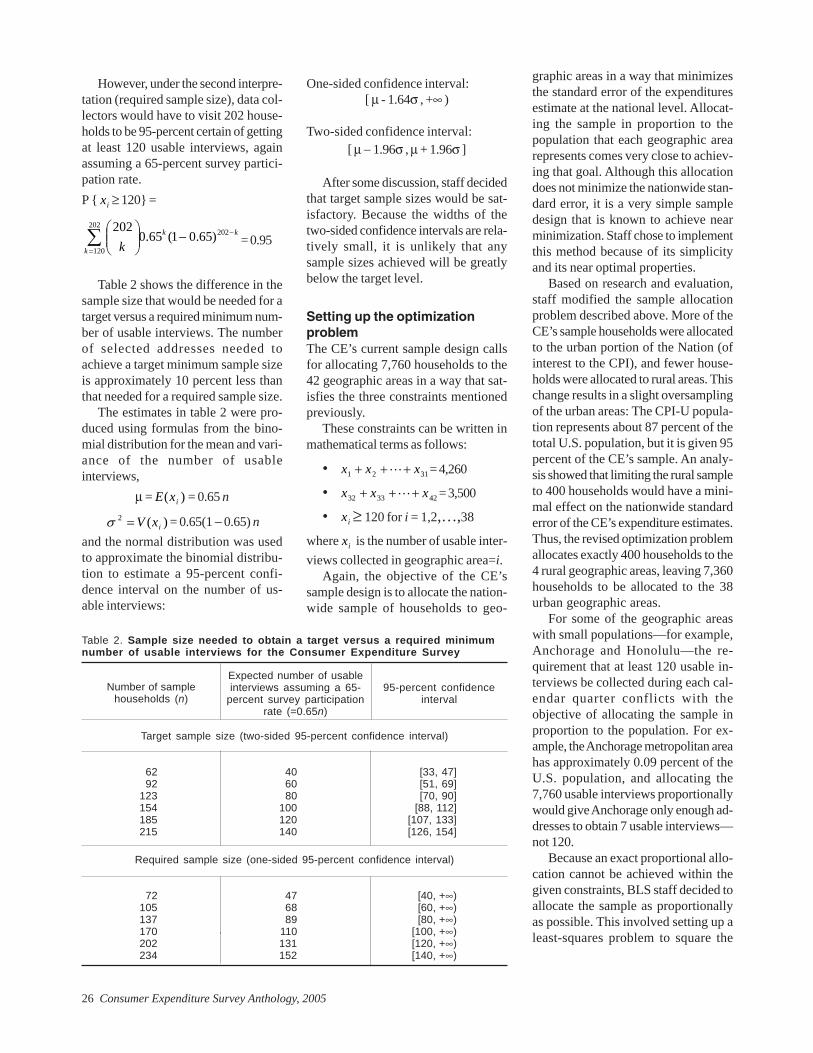
26 Consumer Expenditure Survey Anthology, 2005
However, under the second interpre-tation (required sample size), data col-lectors would have to visit 202 house-holds to be 95-percent certain of gettingat least 120 usable interviews, againassuming a 65-percent survey partici-pation rate.P { ix ≥ 120} =
kk
k k−
=
−⎟⎟⎠
⎞⎜⎜⎝
⎛∑ 202202
120)65.01(65.0
202= 0.95
Table 2 shows the difference in thesample size that would be needed for atarget versus a required minimum num-ber of usable interviews. The numberof selected addresses needed toachieve a target minimum sample sizeis approximately 10 percent less thanthat needed for a required sample size.
The estimates in table 2 were pro-duced using formulas from the bino-mial distribution for the mean and vari-ance of the number of usableinterviews,
µ = )( ixE = 0.65 n
)(2ixV=σ = 0.65(1 − 0.65) n
and the normal distribution was usedto approximate the binomial distribu-tion to estimate a 95-percent confi-dence interval on the number of us-able interviews:
One-sided confidence interval:[ µ - 1.64σ , +∞ )
Two-sided confidence interval:[ µ − 1.96σ , µ + 1.96σ ]
After some discussion, staff decidedthat target sample sizes would be sat-isfactory. Because the widths of thetwo-sided confidence intervals are rela-tively small, it is unlikely that anysample sizes achieved will be greatlybelow the target level.
Setting up the optimizationproblemThe CE’s current sample design callsfor allocating 7,760 households to the42 geographic areas in a way that sat-isfies the three constraints mentionedpreviously.
These constraints can be written inmathematical terms as follows:
• 3121 xxx +++ L = 4,260
• 423332 xxx +++ L = 3,500
• ix ≥ 120 for i = 1,2,…,38
where ix is the number of usable inter-views collected in geographic area=i.
Again, the objective of the CE’ssample design is to allocate the nation-wide sample of households to geo-
graphic areas in a way that minimizesthe standard error of the expendituresestimate at the national level. Allocat-ing the sample in proportion to thepopulation that each geographic arearepresents comes very close to achiev-ing that goal. Although this allocationdoes not minimize the nationwide stan-dard error, it is a very simple sampledesign that is known to achieve nearminimization. Staff chose to implementthis method because of its simplicityand its near optimal properties.
Based on research and evaluation,staff modified the sample allocationproblem described above. More of theCE’s sample households were allocatedto the urban portion of the Nation (ofinterest to the CPI), and fewer house-holds were allocated to rural areas. Thischange results in a slight oversamplingof the urban areas: The CPI-U popula-tion represents about 87 percent of thetotal U.S. population, but it is given 95percent of the CE’s sample. An analy-sis showed that limiting the rural sampleto 400 households would have a mini-mal effect on the nationwide standarderror of the CE’s expenditure estimates.Thus, the revised optimization problemallocates exactly 400 households to the4 rural geographic areas, leaving 7,360households to be allocated to the 38urban geographic areas.
For some of the geographic areaswith small populations—for example,Anchorage and Honolulu—the re-quirement that at least 120 usable in-terviews be collected during each cal-endar quarter conflicts with theobjective of allocating the sample inproportion to the population. For ex-ample, the Anchorage metropolitan areahas approximately 0.09 percent of theU.S. population, and allocating the7,760 usable interviews proportionallywould give Anchorage only enough ad-dresses to obtain 7 usable interviews—not 120.
Because an exact proportional allo-cation cannot be achieved within thegiven constraints, BLS staff decided toallocate the sample as proportionallyas possible. This involved setting up aleast-squares problem to square the
Table 2. Sample size needed to obtain a target versus a required minimumnumber of usable interviews for the Consumer Expenditure Survey
Target sample size (two-sided 95-percent confidence interval)
62 40 [33, 47]92 60 [51, 69]
123 80 [70, 90]154 100 [88, 112]185 120 [107, 133]215 140 [126, 154]
Required sample size (one-sided 95-percent confidence interval)
72 47 [40, +∞)105 68 [60, +∞)137 89 [80, +∞)170 110 [100, +∞)202 131 [120, +∞)234 152 [140, +∞)
Number of samplehouseholds (n)
Expected number of usableinterviews assuming a 65-
percent survey participationrate (=0.65n)
95-percent confidenceinterval
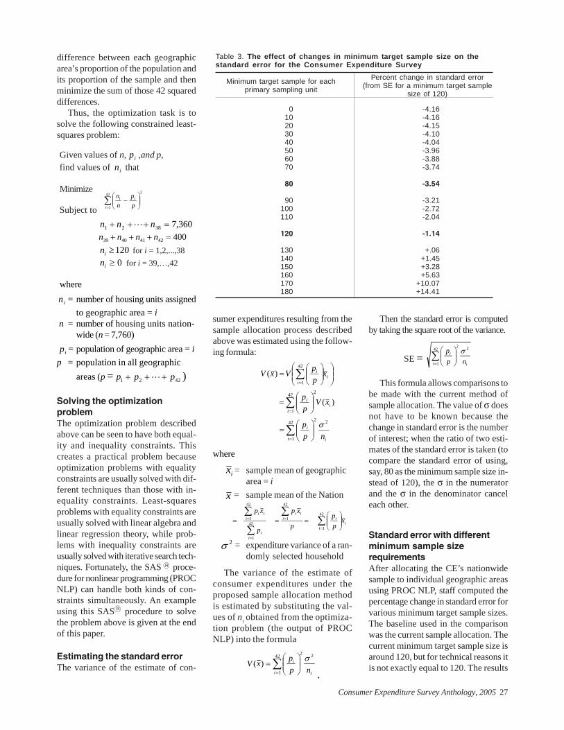
Consumer Expenditure Survey Anthology, 2005 27
difference between each geographicarea’s proportion of the population andits proportion of the sample and thenminimize the sum of those 42 squareddifferences.
Thus, the optimization task is tosolve the following constrained least-squares problem:
Given values of n, ip ,and p,find values of in that
Minimize
Subject to360,73821 =+++ nnn L
120≥in for i = 1,2,...,380≥in for i = 39,…,42
where
in = number of housing units assignedto geographic area = i
n = number of housing units nation-wide (n = 7,760)
ip = population of geographic area = ip = population in all geographic
areas (p = 4221 ppp +++ L )
Solving the optimizationproblemThe optimization problem describedabove can be seen to have both equal-ity and inequality constraints. Thiscreates a practical problem becauseoptimization problems with equalityconstraints are usually solved with dif-ferent techniques than those with in-equality constraints. Least-squaresproblems with equality constraints areusually solved with linear algebra andlinear regression theory, while prob-lems with inequality constraints areusually solved with iterative search tech-niques. Fortunately, the SAS proce-dure for nonlinear programming (PROCNLP) can handle both kinds of con-straints simultaneously. An exampleusing this SAS procedure to solvethe problem above is given at the endof this paper.
Estimating the standard errorThe variance of the estimate of con-
sumer expenditures resulting from thesample allocation process describedabove was estimated using the follow-ing formula:
where
ix = sample mean of geographicarea = i
x = sample mean of the Nation
= expenditure variance of a ran-domly selected household
The variance of the estimate ofconsumer expenditures under theproposed sample allocation methodis estimated by substituting the val-ues of ni obtained from the optimiza-tion problem (the output of PROCNLP) into the formula
∑=
⎟⎟⎠
⎞⎜⎜⎝
⎛=
42
1
22
)(i i
i
nppxV σ
.
Then the standard error is computedby taking the square root of the variance.
SE = ∑=
⎟⎟⎠
⎞⎜⎜⎝
⎛42
1
22
i i
i
npp σ
This formula allows comparisons tobe made with the current method ofsample allocation. The value of σ doesnot have to be known because thechange in standard error is the numberof interest; when the ratio of two esti-mates of the standard error is taken (tocompare the standard error of using,say, 80 as the minimum sample size in-stead of 120), the σ in the numeratorand the σ in the denominator canceleach other.
Standard error with differentminimum sample sizerequirementsAfter allocating the CE’s nationwidesample to individual geographic areasusing PROC NLP, staff computed thepercentage change in standard error forvarious minimum target sample sizes.The baseline used in the comparisonwas the current sample allocation. Thecurrent minimum target sample size isaround 120, but for technical reasons itis not exactly equal to 120. The results
ii
iiii
ii
iii
xpp
p
xp
p
xp∑
∑
∑
∑=
=
=
=⎟⎟⎠
⎞⎜⎜⎝
⎛===
42
1
42
142
1
42
1
2σ
∑=
⎟⎟⎠
⎞⎜⎜⎝
⎛−
42
1
2
i
ii
pp
nn
40042414039 =+++ nnnn
ii
i xppVxV
42
1)( ∑
=⎟⎟⎠
⎞⎜⎜⎝
⎛⎟⎟⎠
⎞⎜⎜⎝
⎛=
Table 3. The effect of changes in minimum target sample size on thestandard error for the Consumer Expenditure Survey
0 -4.1610 -4.16
20 -4.1530 -4.1040 -4.0450 -3.9660 -3.88
70 -3.74
80 -3.54
90 -3.21100 -2.72110 -2.04
120 -1.14
130 +.06140 +1.45150 +3.28160 +5.63170 +10.07180 +14.41
Minimum target sample for eachprimary sampling unit
Percent change in standard error(from SE for a minimum target sample
size of 120)
)(42
1
2
ii
i xVpp∑
=⎟⎟⎠
⎞⎜⎜⎝
⎛=
ii
i
npp 242
1
2σ∑
=⎟⎟⎠
⎞⎜⎜⎝
⎛=
R
R
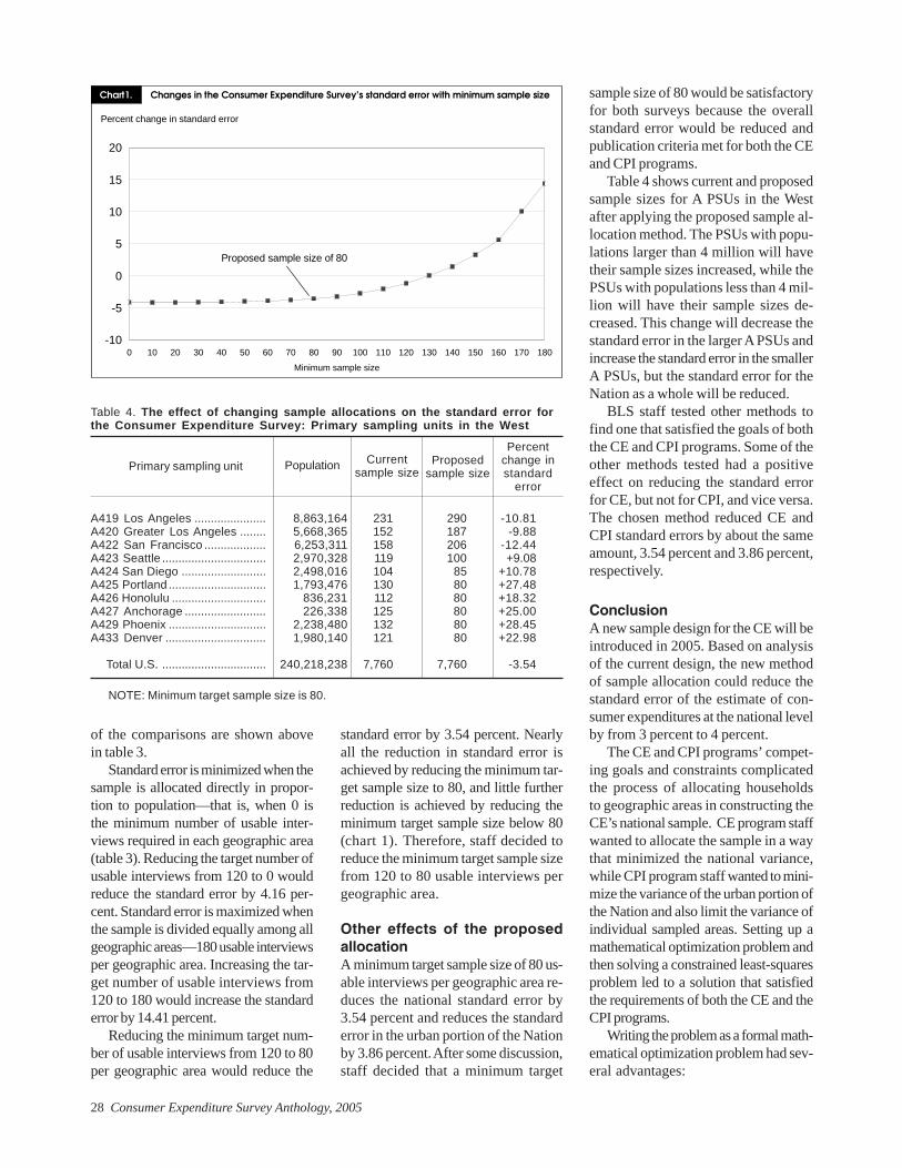
28 Consumer Expenditure Survey Anthology, 2005
sample size of 80 would be satisfactoryfor both surveys because the overallstandard error would be reduced andpublication criteria met for both the CEand CPI programs.
Table 4 shows current and proposedsample sizes for A PSUs in the Westafter applying the proposed sample al-location method. The PSUs with popu-lations larger than 4 million will havetheir sample sizes increased, while thePSUs with populations less than 4 mil-lion will have their sample sizes de-creased. This change will decrease thestandard error in the larger A PSUs andincrease the standard error in the smallerA PSUs, but the standard error for theNation as a whole will be reduced.
BLS staff tested other methods tofind one that satisfied the goals of boththe CE and CPI programs. Some of theother methods tested had a positiveeffect on reducing the standard errorfor CE, but not for CPI, and vice versa.The chosen method reduced CE andCPI standard errors by about the sameamount, 3.54 percent and 3.86 percent,respectively.
ConclusionA new sample design for the CE will beintroduced in 2005. Based on analysisof the current design, the new methodof sample allocation could reduce thestandard error of the estimate of con-sumer expenditures at the national levelby from 3 percent to 4 percent.
The CE and CPI programs’ compet-ing goals and constraints complicatedthe process of allocating householdsto geographic areas in constructing theCE’s national sample. CE program staffwanted to allocate the sample in a waythat minimized the national variance,while CPI program staff wanted to mini-mize the variance of the urban portion ofthe Nation and also limit the variance ofindividual sampled areas. Setting up amathematical optimization problem andthen solving a constrained least-squaresproblem led to a solution that satisfiedthe requirements of both the CE and theCPI programs.
Writing the problem as a formal math-ematical optimization problem had sev-eral advantages:
of the comparisons are shown abovein table 3.
Standard error is minimized when thesample is allocated directly in propor-tion to population—that is, when 0 isthe minimum number of usable inter-views required in each geographic area(table 3). Reducing the target number ofusable interviews from 120 to 0 wouldreduce the standard error by 4.16 per-cent. Standard error is maximized whenthe sample is divided equally among allgeographic areas—180 usable interviewsper geographic area. Increasing the tar-get number of usable interviews from120 to 180 would increase the standarderror by 14.41 percent.
Reducing the minimum target num-ber of usable interviews from 120 to 80per geographic area would reduce the
standard error by 3.54 percent. Nearlyall the reduction in standard error isachieved by reducing the minimum tar-get sample size to 80, and little furtherreduction is achieved by reducing theminimum target sample size below 80(chart 1). Therefore, staff decided toreduce the minimum target sample sizefrom 120 to 80 usable interviews pergeographic area.
Other effects of the proposedallocationA minimum target sample size of 80 us-able interviews per geographic area re-duces the national standard error by3.54 percent and reduces the standarderror in the urban portion of the Nationby 3.86 percent. After some discussion,staff decided that a minimum target
Chart1. Changes in the Consumer Expenditure Survey's standard error with minimum sample size
Percent change in standard error
0 10 20 30 40 50 60 70 80 90 100 110 120 130 140 150 160 170 180
Minimum sample size
-10
-5
0
5
10
15
20
Proposed sample size of 80
Table 4. The effect of changing sample allocations on the standard error forthe Consumer Expenditure Survey: Primary sampling units in the West
A419 Los Angeles ...................... 8,863,164 231 290 -10.81A420 Greater Los Angeles ........ 5,668,365 152 187 -9.88A422 San Francisco ................... 6,253,311 158 206 -12.44A423 Seattle ................................ 2,970,328 119 100 +9.08A424 San Diego .......................... 2,498,016 104 85 +10.78A425 Portland .............................. 1,793,476 130 80 +27.48A426 Honolulu ............................. 836,231 112 80 +18.32A427 Anchorage ......................... 226,338 125 80 +25.00A429 Phoenix .............................. 2,238,480 132 80 +28.45A433 Denver ............................... 1,980,140 121 80 +22.98
Total U.S. ................................ 240,218,238 7,760 7,760 -3.54
NOTE: Minimum target sample size is 80.
Primary sampling unit Population Currentsample size
Proposedsample size
Percentchange instandard
error
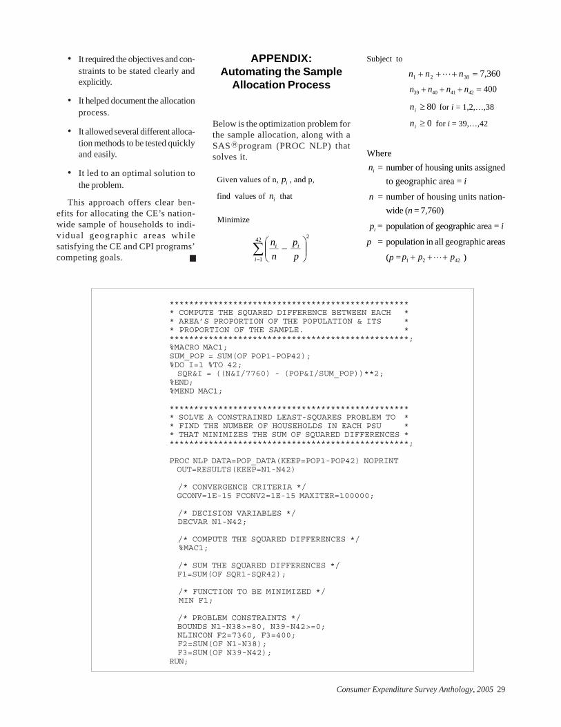
Consumer Expenditure Survey Anthology, 2005 29
• It required the objectives and con-straints to be stated clearly andexplicitly.
• It helped document the allocationprocess.
• It allowed several different alloca-tion methods to be tested quicklyand easily.
• It led to an optimal solution tothe problem.
This approach offers clear ben-efits for allocating the CE’s nation-wide sample of households to indi-vidual geographic areas whilesatisfying the CE and CPI programs’competing goals.
APPENDIX:Automating the Sample
Allocation Process
Below is the optimization problem forthe sample allocation, along with aSAS program (PROC NLP) thatsolves it.
Given values of n, ip , and p,
find values of in that
Minimize
Subject to
360,73821 =+++ nnn L
80≥in for i = 1,2,…,38
0≥in for i = 39,…,42
Where
in = number of housing units assignedto geographic area = i
n = number of housing units nation-wide (n = 7,760)
ip = population of geographic area = i
p = population in all geographic areas
(p = )∑=
⎟⎟⎠
⎞⎜⎜⎝
⎛−
42
1
2
i
ii
pp
nn
40042414039 =+++ nnnn
4221 ppp +++ L
************************************************** COMPUTE THE SQUARED DIFFERENCE BETWEEN EACH ** AREA’S PROPORTION OF THE POPULATION & ITS ** PROPORTION OF THE SAMPLE. **************************************************;%MACRO MAC1;SUM_POP = SUM(OF POP1-POP42);%DO I=1 %TO 42; SQR&I = ((N&I/7760) - (POP&I/SUM_POP))**2;%END;%MEND MAC1;
************************************************** SOLVE A CONSTRAINED LEAST-SQUARES PROBLEM TO ** FIND THE NUMBER OF HOUSEHOLDS IN EACH PSU ** THAT MINIMIZES THE SUM OF SQUARED DIFFERENCES **************************************************;
PROC NLP DATA=POP_DATA(KEEP=POP1-POP42) NOPRINT OUT=RESULTS(KEEP=N1-N42)
/* CONVERGENCE CRITERIA */ GCONV=1E-15 FCONV2=1E-15 MAXITER=100000;
/* DECISION VARIABLES */ DECVAR N1-N42;
/* COMPUTE THE SQUARED DIFFERENCES */ %MAC1;
/* SUM THE SQUARED DIFFERENCES */ F1=SUM(OF SQR1-SQR42);
/* FUNCTION TO BE MINIMIZED */ MIN F1;
/* PROBLEM CONSTRAINTS */ BOUNDS N1-N38>=80, N39-N42>=0; NLINCON F2=7360, F3=400; F2=SUM(OF N1-N38); F3=SUM(OF N39-N42);RUN;
R
30 Consumer Expenditure Survey Anthology, 2005
Part II.Analyses Using Survey Data
Consumer Expenditure Survey Anthology, 2005 31
From AFDC to TANF:Have the New PublicAssistance Laws AffectedConsumer Spending ofRecipients?
Laura Paszkiewicz is an economist in theBranch of Information Analysis, Division ofConsumer Expenditure Surveys, Bureau ofLabor Statistics.
LAURA PASZKIEWICZ IntroductionThe Personal Responsibility and WorkOpportunity Reconciliation Act of 1996(the Welfare Reform Act) replaced theprevious welfare program, Aid to Fami-lies with Dependent Children (AFDC),with a new program, Temporary Assis-tance for Needy Families (TANF). Thenew program gives block grants toStates to design their own welfare pro-grams—provided that they meet cer-tain Federal guidelines. One of the mainrequirements is to limit the amount oftime that a person can receive welfare(hence, temporary assistance).
Since the implementation of the newlaws, numerous research projects haveinvestigated just how well TANF hasbeen doing. Some studies have lookedat how the welfare reform affects dif-ferent groups of people, employmentand earnings, and family structure.
This study looks at how the welfarereform has affected the spending pat-terns of welfare recipients. Looking atspending can give insights into wel-fare recipients’ quality of life.
Using the Consumer ExpenditureSurvey (CE), a comparison of data onwelfare recipients prior to TANF (1988-89), during the transition to TANF(1997-98), and post-TANF (2001-02) wasmade. An analysis of the sample char-acteristics of welfare recipients over thethree time periods was done, as well asan analysis of expenditure patterns.
A brief overview of TANFThe welfare reform established blockgrants for States to develop their ownwelfare programs as long as certain re-quirements were met. States were man-dated to limit the amount of time thatrecipients could receive funds, to re-quire that recipients work when readyor after 24 months of receiving assis-tance, and to establish goals to reduceout-of-wedlock pregnancies.
Prior to the Welfare Reform Act, asfar back as 1987, some States had al-ready established welfare programssimilar to TANF.1 The Welfare ReformAct was passed in 1996 and fully imple-mented in all states by 1998. Data from1997-98 were used to look at TANF’stransition period, and data from 2001-02 were used to look at the post-TANFtime period.
In 2003, TANF was due for reautho-rization in Congress. A bill reauthoriz-ing TANF was passed in the House ofRepresentatives, but not in the Senate.Funding was extended by Congressthrough March of 2005.
1 This article assumes that these Stateswould not have a large effect on the welfarepopulation in the 2 years following the de-velopment of their programs. Due to thedesign of the CE, data from 1988-89 weremore accessible than earlier data (from 1986-87), so these data were used to reflect thewelfare population prior to TANF.
32 Consumer Expenditure Survey Anthology, 2005
The sampleData on welfare receipts are collectedin the income section (section 22) ofthe Interview Survey in the CE. Estab-lished survey participants are asked toanswer the income section of the ques-tionnaire during the second and fifthinterviews. Respondents who replaceoriginal CUs are also asked to reporttheir income for section 22 at the timethat they enter the survey. Income in-formation from the second interview iscarried over to the third and fourth in-terviews.
The screener question about wel-fare has changed over the three timeperiods of interest. For 1988 and 1989(prior to TANF), each respondent wasasked the following question aboutwelfare receipts and other forms of in-come:
“During the past 12 months, did you(or any member of your CU) receiveincome from…worker’s or unemploy-ment compensation; veteran’s pay-ments; public assistance or welfarefrom Federal, State, or local welfareoffices?”
If the respondent replied that he orshe had received some form of assis-tance, he or she was then asked foreach amount individually:
“How much was received from publicassistance or welfare, including moneyreceived from job training grants, suchas Job Corps?”
If a respondent answered affirma-tively to the screener question but didnot know or refused to say the amount,then there was no way to know whichtype of assistance was collected.
The question used during 1997 and1998 (transition to TANF) asked therespondent about welfare assistanceseparately from other forms of assis-tance and grouped the screener ques-tion and the amount question together:
“During the past 12 months, did you(or any member of your CU) receiveincome from…public assistance orwelfare, including money receivedfrom job training grants, such as JobCorps?”
If the respondent answered affirma-tively, the interviewer asked:
“What was the total amount receivedby all CU members?”
For 2001 and 2002 (post TANF), thequestions about welfare were similar tothose used during 1997 and 1998, butthe wording specified the AFDC andJob Corps programs2:
“During the last 12 months, did you(or any member of your CU) receiveany income from…public assistanceor welfare, such as AFDC and grantsfrom Job Corps? Do not include non-monetary assistance, such as foodstamps.”
If the respondent answered affirma-tively, the interviewer asked:
“What was the total amount receivedby all CU members?”
An additional difference in the 2001and 2002 questionnaires was the intro-duction of income ranges or bracketsin section 22. If the respondent did notknow or refused to say the amount ofthe welfare payments received, he orshe would be shown a number of brack-ets and asked to indicate which bracketthe amount fell in. The introduction ofbrackets decreased the percentage ofoverall refusals to the amount question.
The differences in the questionsbetween 1988 and 2002 led to the defi-nition of the welfare sample used in thisstudy. Because the screener questionthat was used in 1988 and 1989 did notseparate welfare payments from otherforms of income, it was not possible toidentify welfare recipients based onthat screener question. Instead, a wel-fare recipient was defined as a personwho reported a positive amount forwelfare assistance (or indicated an in-come bracket for 2001 or 2002) whenasked about specific amounts. Respon-dents in CUs who refused to providean amount or did not know the amountof welfare assistance and would notprovide a bracket (in 2001-02) were ex-cluded from the sample. No othersample restrictions were made.
The sample was weighted to matchthe U.S. population; and, using the
above definition of a welfare recipient,the weighted welfare sample made up3.2 percent of the population in the1988-89 period, 2.3 percent in the 1997-98 period, and 1.4 percent in the 2001-02 period.3 The decreasing percentageof welfare recipients was expected be-cause TANF was designed to give tem-porary assistance. This is consistentwith data on welfare receipts publishedin the 2003 Statistical Abstract, whichshows that the percent of families re-ceiving welfare decreased from 4.1 per-cent in 1988-89 to 3.34 percent in 1997-98, and, then, to 1.91 percent in 2001-02.4
Sample characteristicsIn the 1988-89 period, 83.1 percent ofconsumer units (CUs) who receivedwelfare payments also received someother form of assistance (food stamps,housing assistance, unemploymentcompensation, or worker’s compensa-tion). (See table 1.) This percentagedidn’t change significantly in 1997-98or 2001-02. 5 The largest form of addi-tional assistance among welfare recipi-ents was food stamps. Seventy-eightpercent of welfare recipients also re-ceived food stamps in 1988-89, but thispercentage decreased from 73.1 in 1997-98 to 66.8 percent in 2001-02.6 The Wel-fare Reform Act also imposed somestricter eligibility requirements for re-ceiving food stamps, which may explainsome of the decline in food stamp re-cipients among welfare recipients.Other studies have shown overall de-clines in the numbers of both welfareand non-welfare recipients receivingfood stamps. Percentages of welfarerecipients receiving other forms of as-sistance either increased or trendedupwards over the same three time peri-ods.
2 Although AFDC was discontinued in1996, the CE did not reflect this change until2003.
3 Including the CUs who claimed welfarereceipts but did not know the amount or re-fused to share the amount, welfare recipientsmade up 3.1 percent of the population in1997-98 and 1.6 percent in 2001-02. Thisstatistic is not available for 1988-89.
4 These statistics from the Statistical Ab-stract differ slightly from the CE numbersdue to definitional differences and sampleerror.
5 All significance tests are at the .05 sig-nificance level.
6 Whenever the words “increase or de-crease” are used, the modifier “statisticallysignificant” should be understood.
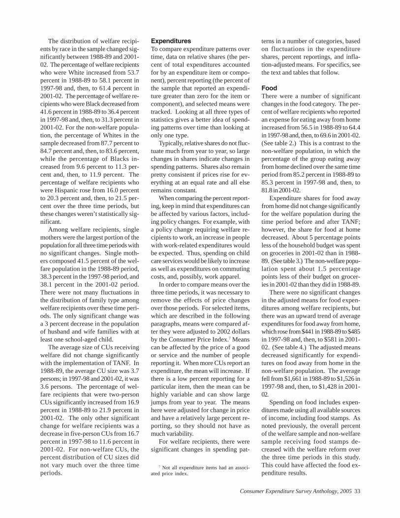
Consumer Expenditure Survey Anthology, 2005 33
The distribution of welfare recipi-ents by race in the sample changed sig-nificantly between 1988-89 and 2001-02. The percentage of welfare recipientswho were White increased from 53.7percent in 1988-89 to 58.1 percent in1997-98 and, then, to 61.4 percent in2001-02. The percentage of welfare re-cipients who were Black decreased from41.6 percent in 1988-89 to 36.4 percentin 1997-98 and, then, to 31.3 percent in2001-02. For the non-welfare popula-tion, the percentage of Whites in thesample decreased from 87.7 percent to84.7 percent and, then, to 83.6 percent,while the percentage of Blacks in-creased from 9.6 percent to 11.3 per-cent and, then, to 11.9 percent. Thepercentage of welfare recipients whowere Hispanic rose from 16.0 percentto 20.3 percent and, then, to 21.5 per-cent over the three time periods, butthese changes weren’t statistically sig-nificant.
Among welfare recipients, singlemothers were the largest portion of thepopulation for all three time periods withno significant changes. Single moth-ers composed 41.5 percent of the wel-fare population in the 1988-89 period,38.3 percent in the 1997-98 period, and38.1 percent in the 2001-02 period.There were not many fluctuations inthe distribution of family type amongwelfare recipients over these time peri-ods. The only significant change wasa 3 percent decrease in the populationof husband and wife families with atleast one school-aged child.
The average size of CUs receivingwelfare did not change significantlywith the implementation of TANF. In1988-89, the average CU size was 3.7persons; in 1997-98 and 2001-02, it was3.6 persons. The percentage of wel-fare recipients that were two-personCUs significantly increased from 16.9percent in 1988-89 to 21.9 percent in2001-02. The only other significantchange for welfare recipients was adecrease in five-person CUs from 16.7percent in 1997-98 to 11.6 percent in2001-02. For non-welfare CUs, thepercent distribution of CU sizes didnot vary much over the three timeperiods.
ExpendituresTo compare expenditure patterns overtime, data on relative shares (the per-cent of total expenditures accountedfor by an expenditure item or compo-nent), percent reporting (the percent ofthe sample that reported an expendi-ture greater than zero for the item orcomponent), and selected means weretracked. Looking at all three types ofstatistics gives a better idea of spend-ing patterns over time than looking atonly one type.
Typically, relative shares do not fluc-tuate much from year to year, so largechanges in shares indicate changes inspending patterns. Shares also remainpretty consistent if prices rise for ev-erything at an equal rate and all elseremains constant.
When comparing the percent report-ing, keep in mind that expenditures canbe affected by various factors, includ-ing policy changes. For example, witha policy change requiring welfare re-cipients to work, an increase in peoplewith work-related expenditures wouldbe expected. Thus, spending on childcare services would be likely to increaseas well as expenditures on commutingcosts, and, possibly, work apparel.
In order to compare means over thethree time periods, it was necessary toremove the effects of price changesover those periods. For selected items,which are described in the followingparagraphs, means were compared af-ter they were adjusted to 2002 dollarsby the Consumer Price Index.7 Meanscan be affected by the price of a goodor service and the number of peoplereporting it. When more CUs report anexpenditure, the mean will increase. Ifthere is a low percent reporting for aparticular item, then the mean can behighly variable and can show largejumps from year to year. The meanshere were adjusted for change in priceand have a relatively large percent re-porting, so they should not have asmuch variability.
For welfare recipients, there weresignificant changes in spending pat-
terns in a number of categories, basedon fluctuations in the expenditureshares, percent reportings, and infla-tion-adjusted means. For specifics, seethe text and tables that follow.
FoodThere were a number of significantchanges in the food category. The per-cent of welfare recipients who reportedan expense for eating away from homeincreased from 56.5 in 1988-89 to 64.4in 1997-98 and, then, to 69.6 in 2001-02.(See table 2.) This is a contrast to thenon-welfare population, in which thepercentage of the group eating awayfrom home declined over the same timeperiod from 85.2 percent in 1988-89 to85.3 percent in 1997-98 and, then, to81.8 in 2001-02.
Expenditure shares for food awayfrom home did not change significantlyfor the welfare population during thetime period before and after TANF;however, the share for food at homedecreased. About 5 percentage pointsless of the household budget was spenton groceries in 2001-02 than in 1988-89. (See table 3.) The non-welfare popu-lation spent about 1.5 percentagepoints less of their budget on grocer-ies in 2001-02 than they did in 1988-89.
There were no significant changesin the adjusted means for food expen-ditures among welfare recipients, butthere was an upward trend of averageexpenditures for food away from home,which rose from $441 in 1988-89 to $485in 1997-98 and, then, to $581 in 2001-02. (See table 4.) The adjusted meansdecreased significantly for expendi-tures on food away from home in thenon-welfare population. The averagefell from $1,661 in 1988-89 to $1,526 in1997-98 and, then, to $1,428 in 2001-02.
Spending on food includes expen-ditures made using all available sourcesof income, including food stamps. Asnoted previously, the overall percentof the welfare sample and non-welfaresample receiving food stamps de-creased with the welfare reform overthe three time periods in this study.This could have affected the food ex-penditure results.
7 Not all expenditure items had an associ-ated price index.
34 Consumer Expenditure Survey Anthology, 2005
HousingAfter the welfare reform, there were alarger number of home owners amongwelfare recipients; the percent report-ing expenditures on owned dwellingsnearly doubled from 13.1 percent in1988-89 to 25.0 percent in 2001-02. Therelative share of total expenditures onowned dwellings also increased, from2.7 percent of the total in 1988-89 to 5.2percent in 2001-02. The non-welfaresample showed similar increases inboth the percent reporting and the rela-tive share spent on owned dwellingsover that time period. In the 1988-89period, 55.3 percent of the non-welfarepopulation reported expenditures onowned dwellings; in the 2001-02 period,66.9 percent reported expenditures onowned dwellings. The relative sharespent on owned dwellings by the non-welfare population rose from 10.9 per-cent in 1988-89 to 13.6 percent in 2001-02. Although the relative shares ofexpenditures on rented dwellings didnot significantly change for eithergroup before and after the implementa-tion of TANF, there was a significantdecrease in the percent of CUs report-ing expenditures on rented dwellingsfor both groups. For the welfare popu-lation, reporting dropped from 82.7 per-cent in 1988-89 to 82.0 percent in 1997-98 and, then, to 72.2 percent in 2001-02;and for non-welfare recipients, report-ing dropped from 35.5 percent in 1988-89 to 33.4 percent in 1997-98 and, then,to 31.6 percent in 2001-02.
TransportationThere were some significant changesin the transportation category of thesurvey. Transportation includes pur-chases of vehicles; vehicle financecharges; vehicle insurance; vehiclerental, leases, and licenses; gas andmotor oil; maintenance and repairs; andpublic transportation. For overalltransportation, there was an increasein the share of total expenditures be-tween 1988-89 and 2001-02; the sharerose from 13.3 percent of total expendi-tures in 1988-89 to 16.0 percent in 1997-98 and, then, to 18.1 percent in 2001-02.There was no significant change inexpenditure shares for non-welfare
recipients. Within the transportationcategory, there was a significant de-crease in percent reporting for usedcars and trucks for the welfare and non-welfare populations; however, sharesof expenditures on used cars and truckstrended upward for the welfare popu-lation and increased for the non-wel-fare population. The percent reportingnew cars and trucks trended upwardbetween 1988-89 and 2001-02 for wel-fare recipients. The percent reportingnew cars and trucks decreased for non-welfare recipients over the same timeperiod. Shares of expenditures on newcars and trucks increased between1988-89 and 2001-02 for welfare recipi-ents from 0.4 percent of total expendi-tures in 1988-89 to 2.1 percent in 2001-02. Shares of expenditures on new carsand trucks decreased for non-welfarerecipients over the same time periodfrom 5.3 percent to 4.5 percent.
Public transportation expendituresremained constant between 1988-89and 1997-98, but showed a significantdrop in expenditure shares and percentreporting for both welfare and non-wel-fare recipients between 1997-98 and2001-02. Public transportation spend-ing includes airfares as well as expen-ditures on buses, trains, and otherforms of mass transit. The time periodafter 9/11 caused a drop in overall ex-penditures on airfares, most likely driv-ing the decrease in overall publictransportation expenditures. A sub-category for public transportation wasavailable only for 1997-98 and 2001-02,which includes data on intracity masstransit, taxis and limousines, andschool buses (excluding all publictransportation expenditures on trips).8
Data available between 1997-98 and2001-02 indicate that the share of totalexpenditures spent on intracity masstransit, taxi fares and limousines, andschool buses by the welfare popula-tion decreased from 0.2 percent to 0.1percent between 1997-98 and 2001-02.The percent reporting expenditures forthese items also declined from 4.4 per-cent to 2.9 percent.
With the work requirement for wel-fare recipients that was instituted withthe 1996 legislation, welfare recipientswere expected to have more transpor-tation expenditures due to the neces-sity of commuting. Data indicate thatvehicle purchases and operating expen-ditures increased for welfare recipientsfrom before to after the welfare reform,even though public transportation ex-penditures decreased.
Child careWith the new work requirements for re-ceiving TANF benefits and the largepercentage of single parents receivingbenefits, expenditures on child carewere expected to increase. While therewere no significant changes for thewelfare population, the percent report-ing an expenditure for child caretrended upward from 8.8 percent in1988-89 to 10.6 percent in 2001-02. Al-ternately, percent reporting for childcare by the non-welfare population de-creased over the three time periods with10.0 percent reporting in the 1988-89period, 8.8 percent reporting in the1997-98 period, and 8.1 percent report-ing in the 2001-02 period. There wereno significant changes in expenditureshares for child care in either group.
EntertainmentBefore the welfare reform, 70.2 percentof welfare recipients reported an expen-diture on entertainment. The percent-age rose to 82.1 in 1997-98 and to 83.5percent in 2001-02. For non-welfarerecipients, the percent reporting alsoincreased overall, rising from 86.7 per-cent in 1988-89 to 90.0 percent in 1997-98, but, then, remaining about the samefor 2001-02. A large part of the changein the percent reporting appears to befrom the purchase of televisions, radios,and sound equipment. The percent ofwelfare recipients reporting an expen-diture on that component rose from 49.8percent to 72.3 percent between 1988-89 and 2001-02. For non-welfare recipi-ents, spending on that component rosefrom 70 to 81.8 percent over the sametime period. There were no significantchanges in the expenditure shares ofoverall entertainment expenditures for
8 Trips are defined as any overnight tripsor day trips of 75 or more miles.
Consumer Expenditure Survey Anthology, 2005 35
either group during that time period;however, the non-welfare recipients’ ex-penditure share on televisions, radios,and sound equipment rose slightly.
ApparelThere were not many significant differ-ences in percent reporting or in expen-diture shares on apparel for the welfaresample. Overall, the total share on ap-parel decreased between 1988-89 and2001-02 from 6.9 percent to 5.2 percentof total expenditures, respectively. Thetwo significant differences in sharesamong the subcomponents were forfootwear expenditures and for men’sand boys’ apparel expenditures: bothhad a significant decrease. Footwearexpenditures also showed the only de-crease in percent reporting for the wel-fare sample. Although there were notmany significant changes, the welfarepopulation showed similar trends to thespending patterns of the non-welfarepopulation. For the non-welfare popu-lation, the percentage of CUs report-ing and the shares of expenditures de-
creased for most of the apparel sub-components.
OtherA number of other categories showedsignificant changes between the pre-TANF and post-TANF welfare period.The percent of CUs reporting spend-ing on health insurance increased forthe welfare and non-welfare popula-tions between 1988-89 and 2001-02. Forwelfare recipients, the percent report-ing health insurance rose from 14.9 per-cent in 1988-89 to 20.1 percent in 1997-98 and, then, to 24.6 percent in 2001-02.For the non-welfare group, these per-centages were 57.0 percent, 63.8 per-cent, and 63.0 percent, respectively.The share of expenditures on health in-surance also increased over that timeperiod for both groups. The welfaregroup allocated 0.7 percent of their to-tal expenditures to health insurance in1988-89. This share went from 1.1 per-cent in 1997-98 to 1.6 percent in 2001-02. The non-welfare group allocated2.0 percent of their total expenditures
to health insurance in 1988-89, 2.8 per-cent in 1997-98, and 3.0 percent in 2001-02. For expenditures on life and otherpersonal insurance, the percent report-ing decreased for both groups, and theexpenditure shares also decreased forboth groups.
ConclusionOverall, there were some significantchanges in spending by welfare recipi-ents from the pre-TANF to post-TANFperiod. Many changes for the welfarepopulation, such as the change fromrenting to owning, have followed thetrends of the non-welfare population.Other changes in the spending pat-terns of welfare recipients, such as ex-penditures on food away from home,have been different from the trends ofthe non-welfare recipients. While itmay not be possible to definitely at-tribute the reason for changes in spend-ing to the introduction of TANF, CEdata show that there were some sig-nificant changes from the pre-TANF tothe post-TANF period.
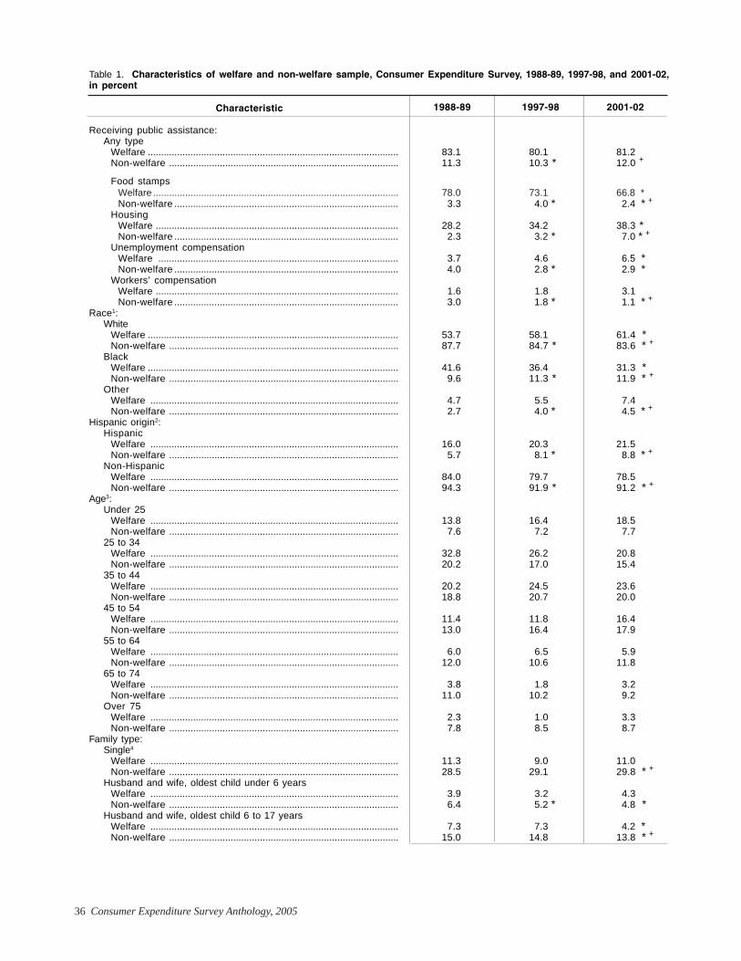
36 Consumer Expenditure Survey Anthology, 2005
Table 1. Characteristics of welfare and non-welfare sample, Consumer Expenditure Survey, 1988-89, 1997-98, and 2001-02,in percent
Receiving public assistance:Any type
Welfare .............................................................................................. 83.1 80.1 81.2Non-welfare ...................................................................................... 11.3 10.3 * 12.0 +
Food stampsWelfare ............................................................................................ 78.0 73.1 66.8 *Non-welfare .................................................................................... 3.3 4.0 * 2.4 * +
HousingWelfare ........................................................................................... 28.2 34.2 38.3 *Non-welfare .................................................................................... 2.3 3.2 * 7.0 * +
Unemployment compensationWelfare .......................................................................................... 3.7 4.6 6.5 *Non-welfare .................................................................................... 4.0 2.8 * 2.9 *
Workers’ compensationWelfare ........................................................................................... 1.6 1.8 3.1Non-welfare .................................................................................... 3.0 1.8 * 1.1 * +
Race1:White
Welfare .............................................................................................. 53.7 58.1 61.4 *Non-welfare ...................................................................................... 87.7 84.7 * 83.6 * +
BlackWelfare .............................................................................................. 41.6 36.4 31.3 *Non-welfare ...................................................................................... 9.6 11.3 * 11.9 * +
OtherWelfare ............................................................................................. 4.7 5.5 7.4Non-welfare ...................................................................................... 2.7 4.0 * 4.5 * +
Hispanic origin2:Hispanic
Welfare ............................................................................................. 16.0 20.3 21.5Non-welfare ...................................................................................... 5.7 8.1 * 8.8 * +
Non-HispanicWelfare ............................................................................................. 84.0 79.7 78.5Non-welfare ...................................................................................... 94.3 91.9 * 91.2 * +
Age3:Under 25
Welfare ............................................................................................. 13.8 16.4 18.5Non-welfare ...................................................................................... 7.6 7.2 7.7
25 to 34Welfare ............................................................................................. 32.8 26.2 20.8Non-welfare ...................................................................................... 20.2 17.0 15.4
35 to 44Welfare ............................................................................................. 20.2 24.5 23.6Non-welfare ...................................................................................... 18.8 20.7 20.0
45 to 54Welfare ............................................................................................. 11.4 11.8 16.4Non-welfare ...................................................................................... 13.0 16.4 17.9
55 to 64Welfare ............................................................................................. 6.0 6.5 5.9Non-welfare ...................................................................................... 12.0 10.6 11.8
65 to 74Welfare ............................................................................................. 3.8 1.8 3.2Non-welfare ...................................................................................... 11.0 10.2 9.2
Over 75Welfare ............................................................................................. 2.3 1.0 3.3Non-welfare ...................................................................................... 7.8 8.5 8.7
Family type:Single4
Welfare ............................................................................................. 11.3 9.0 11.0Non-welfare ...................................................................................... 28.5 29.1 29.8 * +
Husband and wife, oldest child under 6 yearsWelfare ............................................................................................. 3.9 3.2 4.3Non-welfare ...................................................................................... 6.4 5.2 * 4.8 *
Husband and wife, oldest child 6 to 17 yearsWelfare ............................................................................................. 7.3 7.3 4.2 *Non-welfare ...................................................................................... 15.0 14.8 13.8 * +
2001-021997-981988-89Characteristic
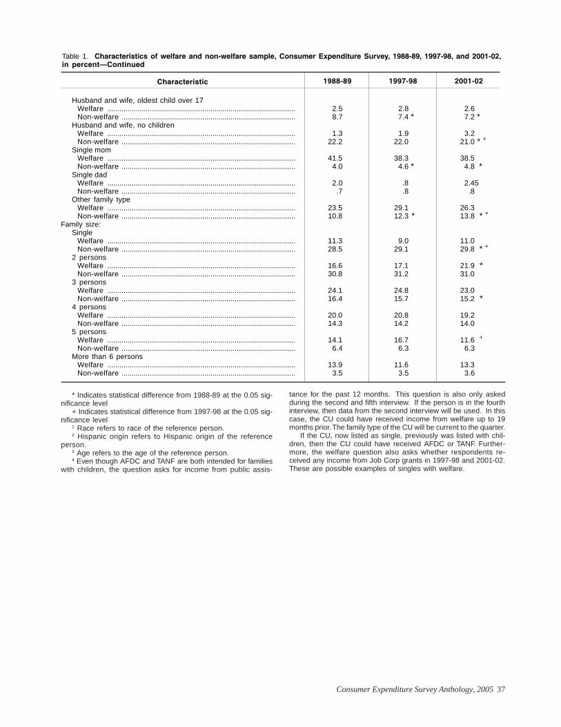
Consumer Expenditure Survey Anthology, 2005 37
Husband and wife, oldest child over 17Welfare ............................................................................................. 2.5 2.8 2.6Non-welfare ...................................................................................... 8.7 7.4 * 7.2 *
Husband and wife, no childrenWelfare ............................................................................................. 1.3 1.9 3.2Non-welfare ...................................................................................... 22.2 22.0 21.0 * +
Single momWelfare ............................................................................................. 41.5 38.3 38.5Non-welfare ...................................................................................... 4.0 4.6 * 4.8 *
Single dadWelfare ............................................................................................. 2.0 .8 2.45Non-welfare ...................................................................................... .7 .8 .8
Other family typeWelfare ............................................................................................. 23.5 29.1 26.3Non-welfare ...................................................................................... 10.8 12.3 * 13.8 * +
Family size:Single
Welfare ............................................................................................. 11.3 9.0 11.0Non-welfare ...................................................................................... 28.5 29.1 29.8 * +
2 personsWelfare ............................................................................................. 16.6 17.1 21.9 *Non-welfare ...................................................................................... 30.8 31.2 31.0
3 personsWelfare ............................................................................................. 24.1 24.8 23.0Non-welfare ...................................................................................... 16.4 15.7 15.2 *
4 personsWelfare ............................................................................................. 20.0 20.8 19.2Non-welfare ...................................................................................... 14.3 14.2 14.0
5 personsWelfare ............................................................................................. 14.1 16.7 11.6 +
Non-welfare ...................................................................................... 6.4 6.3 6.3More than 6 persons
Welfare ............................................................................................. 13.9 11.6 13.3Non-welfare ...................................................................................... 3.5 3.5 3.6
Table 1. Characteristics of welfare and non-welfare sample, Consumer Expenditure Survey, 1988-89, 1997-98, and 2001-02,in percent—Continued
2001-021997-981988-89
* Indicates statistical difference from 1988-89 at the 0.05 sig-nificance level
+ Indicates statistical difference from 1997-98 at the 0.05 sig-nificance level
1 Race refers to race of the reference person.2 Hispanic origin refers to Hispanic origin of the reference
person.3 Age refers to the age of the reference person.4 Even though AFDC and TANF are both intended for families
with children, the question asks for income from public assis-
Characteristic
tance for the past 12 months. This question is also only askedduring the second and fifth interview. If the person is in the fourthinterview, then data from the second interview will be used. In thiscase, the CU could have received income from welfare up to 19months prior. The family type of the CU will be current to the quarter.
If the CU, now listed as single, previously was listed with chil-dren, then the CU could have received AFDC or TANF. Further-more, the welfare question also asks whether respondents re-ceived any income from Job Corp grants in 1997-98 and 2001-02.These are possible examples of singles with welfare.
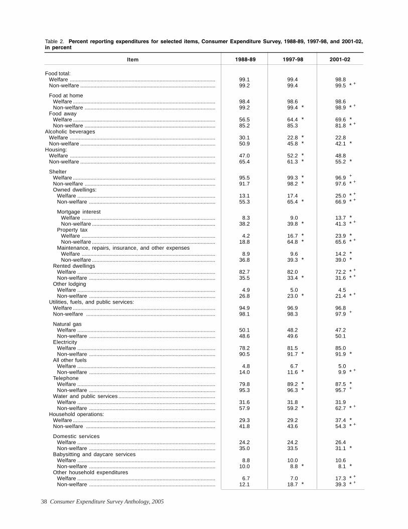
38 Consumer Expenditure Survey Anthology, 2005
Food total:Welfare ................................................................................................... 99.1 99.4 98.8Non-welfare ............................................................................................ 99.2 99.4 99.5 * +
Food at homeWelfare ................................................................................................. 98.4 98.6 98.6Non-welfare ......................................................................................... 99.2 99.4 * 98.9 * +
Food awayWelfare ................................................................................................. 56.5 64.4 * 69.6 *Non-welfare ......................................................................................... 85.2 85.3 81.8 * +
Alcoholic beveragesWelfare ................................................................................................... 30.1 22.8 * 22.8Non-welfare ............................................................................................ 50.9 45.8 * 42.1 *
Housing:Welfare ................................................................................................... 47.0 52.2 * 48.8Non-welfare ............................................................................................ 65.4 61.3 * 55.2 *
ShelterWelfare ................................................................................................. 95.5 99.3 * 96.9 +
Non-welfare ......................................................................................... 91.7 98.2 * 97.6 * +
Owned dwellings:Welfare .............................................................................................. 13.1 17.4 25.0 * +
Non-welfare ...................................................................................... 55.3 65.4 * 66.9 * +
Mortgage interestWelfare ........................................................................................... 8.3 9.0 13.7 *Non-welfare .................................................................................... 38.2 39.8 * 41.3 * +
Property taxWelfare ........................................................................................... 4.2 16.7 * 23.9 *Non-welfare .................................................................................... 18.8 64.8 * 65.6 * +
Maintenance, repairs, insurance, and other expensesWelfare ........................................................................................... 8.9 9.6 14.2 *Non-welfare .................................................................................... 36.8 39.3 * 39.0 *
Rented dwellingsWelfare .............................................................................................. 82.7 82.0 72.2 * +
Non-welfare ...................................................................................... 35.5 33.4 * 31.6 * +
Other lodgingWelfare .............................................................................................. 4.9 5.0 4.5Non-welfare ...................................................................................... 26.8 23.0 * 21.4 * +
Utilities, fuels, and public services:Welfare ................................................................................................. 94.9 96.9 96.8Non-welfare ........................................................................................ 98.1 98.3 97.9 +
Natural gasWelfare .............................................................................................. 50.1 48.2 47.2Non-welfare ...................................................................................... 48.6 49.6 50.1
ElectricityWelfare .............................................................................................. 78.2 81.5 85.0Non-welfare ...................................................................................... 90.5 91.7 * 91.9 *
All other fuelsWelfare .............................................................................................. 4.8 6.7 5.0Non-welfare ...................................................................................... 14.0 11.6 * 9.9 * +
TelephoneWelfare .............................................................................................. 79.8 89.2 * 87.5 *Non-welfare ...................................................................................... 95.3 96.3 * 95.7 +
Water and public services ..................................................................Welfare .............................................................................................. 31.6 31.8 31.9Non-welfare ...................................................................................... 57.9 59.2 * 62.7 * +
Household operations:Welfare ................................................................................................. 29.3 29.2 37.4 *Non-welfare ........................................................................................ 41.8 43.6 54.3 * +
Domestic servicesWelfare .............................................................................................. 24.2 24.2 26.4Non-welfare ...................................................................................... 35.0 33.5 31.1 *
Babysitting and daycare servicesWelfare .............................................................................................. 8.8 10.0 10.6Non-welfare ...................................................................................... 10.0 8.8 * 8.1 *
Other household expendituresWelfare .............................................................................................. 6.7 7.0 17.3 * +
Non-welfare ...................................................................................... 12.1 18.7 * 39.3 * +
Table 2. Percent reporting expenditures for selected items, Consumer Expenditure Survey, 1988-89, 1997-98, and 2001-02,in percent
2001-021997-981988-89Item
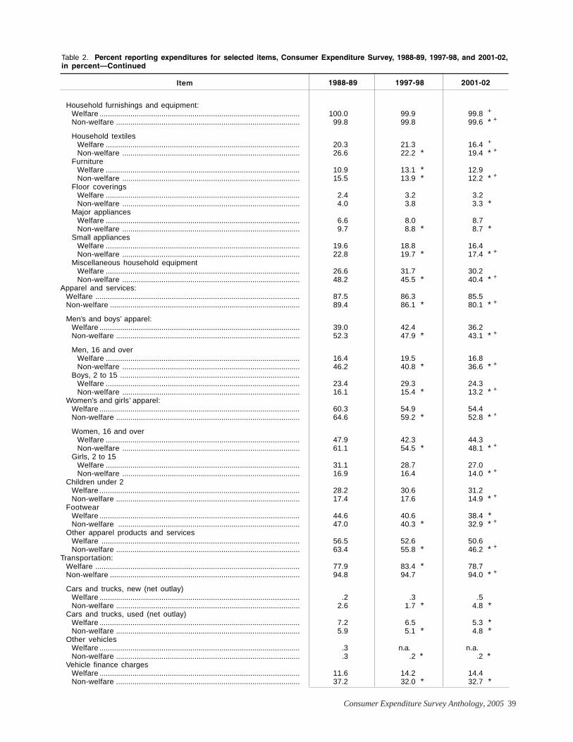
Consumer Expenditure Survey Anthology, 2005 39
Household furnishings and equipment:Welfare ................................................................................................. 100.0 99.9 99.8 +
Non-welfare ......................................................................................... 99.8 99.8 99.6 * +
Household textilesWelfare .............................................................................................. 20.3 21.3 16.4 +
Non-welfare ...................................................................................... 26.6 22.2 * 19.4 * +
FurnitureWelfare .............................................................................................. 10.9 13.1 * 12.9Non-welfare ...................................................................................... 15.5 13.9 * 12.2 * +
Floor coveringsWelfare .............................................................................................. 2.4 3.2 3.2Non-welfare ...................................................................................... 4.0 3.8 3.3 *
Major appliancesWelfare .............................................................................................. 6.6 8.0 8.7Non-welfare ...................................................................................... 9.7 8.8 * 8.7 *
Small appliancesWelfare .............................................................................................. 19.6 18.8 16.4Non-welfare ...................................................................................... 22.8 19.7 * 17.4 * +
Miscellaneous household equipmentWelfare .............................................................................................. 26.6 31.7 30.2Non-welfare ...................................................................................... 48.2 45.5 * 40.4 * +
Apparel and services:Welfare ................................................................................................... 87.5 86.3 85.5Non-welfare ............................................................................................ 89.4 86.1 * 80.1 * +
Men’s and boys’ apparel:Welfare ................................................................................................. 39.0 42.4 36.2Non-welfare ......................................................................................... 52.3 47.9 * 43.1 * +
Men, 16 and overWelfare .............................................................................................. 16.4 19.5 16.8Non-welfare ...................................................................................... 46.2 40.8 * 36.6 * +
Boys, 2 to 15 .......................................................................................Welfare .............................................................................................. 23.4 29.3 24.3Non-welfare ...................................................................................... 16.1 15.4 * 13.2 * +
Women’s and girls’ apparel:Welfare ................................................................................................. 60.3 54.9 54.4Non-welfare ......................................................................................... 64.6 59.2 * 52.8 * +
Women, 16 and overWelfare .............................................................................................. 47.9 42.3 44.3Non-welfare ...................................................................................... 61.1 54.5 * 48.1 * +
Girls, 2 to 15Welfare .............................................................................................. 31.1 28.7 27.0Non-welfare ...................................................................................... 16.9 16.4 14.0 * +
Children under 2Welfare ................................................................................................. 28.2 30.6 31.2Non-welfare ......................................................................................... 17.4 17.6 14.9 * +
FootwearWelfare ................................................................................................. 44.6 40.6 38.4 *Non-welfare ........................................................................................ 47.0 40.3 * 32.9 * +
Other apparel products and servicesWelfare ................................................................................................ 56.5 52.6 50.6Non-welfare ......................................................................................... 63.4 55.8 * 46.2 * +
Transportation:Welfare ................................................................................................... 77.9 83.4 * 78.7Non-welfare ............................................................................................ 94.8 94.7 94.0 * +
Cars and trucks, new (net outlay)Welfare ................................................................................................. .2 .3 .5Non-welfare ......................................................................................... 2.6 1.7 * 4.8 *
Cars and trucks, used (net outlay)Welfare ................................................................................................. 7.2 6.5 5.3 *Non-welfare ......................................................................................... 5.9 5.1 * 4.8 *
Other vehiclesWelfare ................................................................................................. .3 n.a. n.a.Non-welfare ......................................................................................... .3 .2 * .2 *
Vehicle finance chargesWelfare ................................................................................................. 11.6 14.2 14.4Non-welfare ......................................................................................... 37.2 32.0 * 32.7 *
Table 2. Percent reporting expenditures for selected items, Consumer Expenditure Survey, 1988-89, 1997-98, and 2001-02,in percent—Continued
2001-021997-981988-89Item
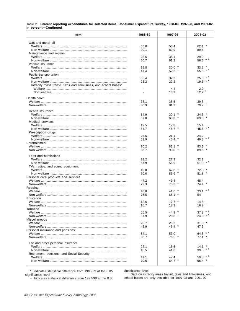
40 Consumer Expenditure Survey Anthology, 2005
Table 2. Percent reporting expenditures for selected items, Consumer Expenditure Survey, 1988-89, 1997-98, and 2001-02,in percent—Continued
Gas and motor oilWelfare ................................................................................................ 53.8 58.4 62.1 *Non-welfare ......................................................................................... 90.1 89.9 89.4
Maintenance and repairsWelfare ................................................................................................. 28.6 35.1 29.9Non-welfare ......................................................................................... 60.7 61.2 56.6 * +
Vehicle insuranceWelfare ................................................................................................ 19.8 30.0 * 33.2 *Non-welfare ......................................................................................... 47.4 52.3 * 55.6 * +
Public transportationWelfare ................................................................................................. 33.4 32.3 25.0 * +
Non-welfare ......................................................................................... 23.2 22.2 19.8 * +
Intracity mass transit, taxis and limousines, and school buses1
Welfare .............................................................................................. - 4.4 2.9Non-welfare ...................................................................................... - 13.9 12.2 +
Health care:Welfare ................................................................................................... 38.1 38.6 39.8Non-welfare ............................................................................................ 80.9 81.3 79.7 +
Health insuranceWelfare ................................................................................................. 14.9 20.1 * 24.6 *Non-welfare ........................................................................................ 57.0 63.8 * 63.0 *
Medical servicesWelfare ................................................................................................. 19.5 17.8 15.4Non-welfare ......................................................................................... 54.7 48.7 * 45.5 * +
Prescription drugsWelfare ................................................................................................. 25.5 21.1 24.2Non-welfare ......................................................................................... 52.9 46.4 * 49.3 * +
Entertainment:Welfare ................................................................................................... 70.2 82.1 * 83.5 *Non-welfare ............................................................................................ 86.7 90.0 * 89.6 *
Fees and admissionsWelfare ................................................................................................. 28.2 27.3 32.2Non-welfare ........................................................................................ 57.9 56.9 51.0 * +
TVs, radios, and sound equipmentWelfare ................................................................................................. 49.8 67.8 * 72.3 *Non-welfare ........................................................................................ 70.0 81.6 * 81.8 *
Personal care products and servicesWelfare ................................................................................................... 47.2 49.4 48.4Non-welfare ............................................................................................ 79.3 75.3 * 74.4 *
ReadingWelfare ................................................................................................... 48.8 41.6 * 33.1 * +
Non-welfare ............................................................................................ 76.5 65.1 * 54Education
Welfare ................................................................................................... 12.6 17.7 * 14.8Non-welfare ............................................................................................ 16.7 18.3 16.9 +
TobaccoWelfare ................................................................................................... 55.5 44.9 * 37.3 * +
Non-welfare ............................................................................................ 37.9 28.8 * 24.3 * +
MiscellaneousWelfare ................................................................................................... 20.7 25.3 31.3 *Non-welfare ............................................................................................ 48.9 46.4 * 47.3
Personal insurance and pensions:Welfare ................................................................................................... 54.1 53.0 64.6 * +
Non-welfare ............................................................................................ 80.7 76.5 * 77.1 *
Life and other personal insuranceWelfare ................................................................................................. 22.1 16.6 14.1 *Non-welfare ......................................................................................... 45.5 41.6 39.5 * +
Retirement, pensions, and Social SecurityWelfare ................................................................................................. 41.1 47.4 59.3 * +
Non-welfare ......................................................................................... 70.6 64.7 * 66.4 *
* Indicates statistical difference from 1988-89 at the 0.05significance level
+ Indicates statistical difference from 1997-98 at the 0.05
significance level1 Data on intracity mass transit, taxis and limousines, and
school buses are only available for 1997-98 and 2001-02.
2001-021997-981988-89Item
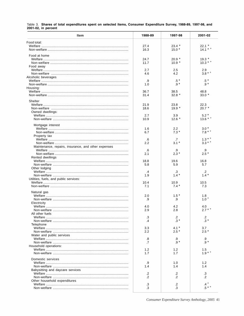
Consumer Expenditure Survey Anthology, 2005 41
Food total:Welfare ................................................................................................... 27.4 23.4 * 22.1 *Non-welfare ............................................................................................ 16.3 15.0 * 14.1 * +
Food at homeWelfare ................................................................................................. 24.7 20.9 * 19.3 *Non-welfare ......................................................................................... 11.7 10.9 * 10.3 * +
Food awayWelfare ................................................................................................. 2.7 2.5 2.9Non-welfare ........................................................................................ 4.6 4.2 3.8 * +
Alcoholic beveragesWelfare ................................................................................................... .9 .5 * .5 *Non-welfare ............................................................................................ 1.0 .9 * .9 *
Housing:Welfare ................................................................................................... 36.7 38.5 48.8Non-welfare ............................................................................................ 31.4 32.8 * 33.0 *
ShelterWelfare ................................................................................................. 21.9 23.8 22.3Non-welfare ........................................................................................ 18.6 19.9 * 20.7 *Owned dwellings:
Welfare .............................................................................................. 2.7 3.9 5.2 *Non-welfare ...................................................................................... 10.9 12.6 * 13.6 * +
Mortgage interestWelfare ........................................................................................... 1.6 2.2 3.0 *Non-welfare .................................................................................... 6.7 7.3 * 7.8 * +
Property taxWelfare ........................................................................................... .6 .7 1.3 * +
Non-welfare .................................................................................... 2.2 3.1 * 3.3 * +
Maintenance, repairs, insurance, and other expensesWelfare ........................................................................................... .6 .9 .9Non-welfare .................................................................................... 2.1 2.3 * 2.5 *
Rented dwellingsWelfare .............................................................................................. 18.8 19.6 16.8Non-welfare ...................................................................................... 5.8 5.9 5.7
Other lodgingWelfare .............................................................................................. .4 .3 .2Non-welfare ...................................................................................... 1.9 1.4 * 1.4 *
Utilities, fuels, and public services:Welfare ................................................................................................. 10.4 10.9 10.5Non-welfare ......................................................................................... 7.1 7.4 * 7.3
Natural gasWelfare .............................................................................................. 2.0 1.5 * 1.8Non-welfare ...................................................................................... .9 .9 1.0 +
ElectricityWelfare .............................................................................................. 4.0 4.2 4.0Non-welfare ...................................................................................... 2.9 2.8 2.7 * +
All other fuelsWelfare .............................................................................................. .3 .2 .2Non-welfare ...................................................................................... .4 .3 * .3 *
TelephoneWelfare .............................................................................................. 3.3 4.1 * 3.7Non-welfare ...................................................................................... 2.2 2.5 * 2.5 *
Water and public servicesWelfare .............................................................................................. .8 .9 .9Non-welfare ...................................................................................... .7 .9 * .9 *
Household operations:Welfare .............................................................................................. 1.2 1.2 1.5Non-welfare ...................................................................................... 1.7 1.7 1.9 * +
Domestic servicesWelfare .............................................................................................. .9 1.0 1.2Non-welfare ...................................................................................... 1.4 1.4 1.4
Babysitting and daycare servicesWelfare .............................................................................................. .2 .2 .3Non-welfare ...................................................................................... .2 .2 .2
Other household expendituresWelfare .............................................................................................. .3 .2 .4 +
Non-welfare ...................................................................................... .3 .3 .5 * +
2001-021997-981988-89Item
Table 3. Shares of total expenditures spent on selected items, Consumer Expenditure Survey, 1988-89, 1997-98, and2001-02, in percent
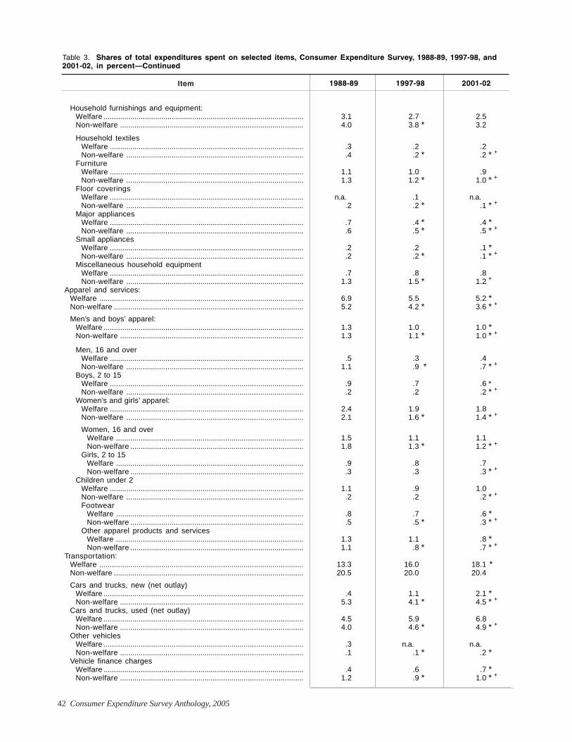
42 Consumer Expenditure Survey Anthology, 2005
Household furnishings and equipment:Welfare ................................................................................................. 3.1 2.7 2.5Non-welfare ......................................................................................... 4.0 3.8 * 3.2
Household textilesWelfare .............................................................................................. .3 .2 .2Non-welfare ...................................................................................... .4 .2 * .2 * +
FurnitureWelfare .............................................................................................. 1.1 1.0 .9Non-welfare ...................................................................................... 1.3 1.2 * 1.0 * +
Floor coveringsWelfare .............................................................................................. n.a. .1 n.a.Non-welfare ...................................................................................... .2 .2 * .1 * +
Major appliancesWelfare .............................................................................................. .7 .4 * .4 *Non-welfare ...................................................................................... .6 .5 * .5 * +
Small appliancesWelfare .............................................................................................. .2 .2 .1 *Non-welfare ...................................................................................... .2 .2 * .1 * +
Miscellaneous household equipmentWelfare .............................................................................................. .7 .8 .8Non-welfare ...................................................................................... 1.3 1.5 * 1.2 +
Apparel and services:Welfare ................................................................................................... 6.9 5.5 5.2 *Non-welfare ............................................................................................ 5.2 4.2 * 3.6 * +
Men’s and boys’ apparel:Welfare ................................................................................................. 1.3 1.0 1.0 *Non-welfare ......................................................................................... 1.3 1.1 * 1.0 * +
Men, 16 and overWelfare .............................................................................................. .5 .3 .4Non-welfare ...................................................................................... 1.1 .9 * .7 * +
Boys, 2 to 15Welfare .............................................................................................. .9 .7 .6 *Non-welfare ...................................................................................... .2 .2 .2 * +
Women’s and girls’ apparel:Welfare .............................................................................................. 2.4 1.9 1.8Non-welfare ...................................................................................... 2.1 1.6 * 1.4 * +
Women, 16 and overWelfare ........................................................................................... 1.5 1.1 1.1Non-welfare .................................................................................... 1.8 1.3 * 1.2 * +
Girls, 2 to 15Welfare ........................................................................................... .9 .8 .7Non-welfare .................................................................................... .3 .3 .3 * +
Children under 2Welfare .............................................................................................. 1.1 .9 1.0Non-welfare ...................................................................................... .2 .2 .2 * +
FootwearWelfare ........................................................................................... .8 .7 .6 *Non-welfare .................................................................................... .5 .5 * .3 * +
Other apparel products and servicesWelfare ........................................................................................... 1.3 1.1 .8 *Non-welfare .................................................................................... 1.1 .8 * .7 * +
Transportation:Welfare ................................................................................................... 13.3 16.0 18.1 *Non-welfare ............................................................................................ 20.5 20.0 20.4
Cars and trucks, new (net outlay)Welfare ................................................................................................. .4 1.1 2.1 *Non-welfare ......................................................................................... 5.3 4.1 * 4.5 * +
Cars and trucks, used (net outlay)Welfare ................................................................................................. 4.5 5.9 6.8Non-welfare ......................................................................................... 4.0 4.6 * 4.9 * +
Other vehiclesWelfare ................................................................................................. .3 n.a. n.a.Non-welfare ......................................................................................... .1 .1 * .2 *
Vehicle finance chargesWelfare ................................................................................................. .4 .6 .7 *Non-welfare ......................................................................................... 1.2 .9 * 1.0 * +
Table 3. Shares of total expenditures spent on selected items, Consumer Expenditure Survey, 1988-89, 1997-98, and2001-02, in percent—Continued
2001-021997-981988-89Item
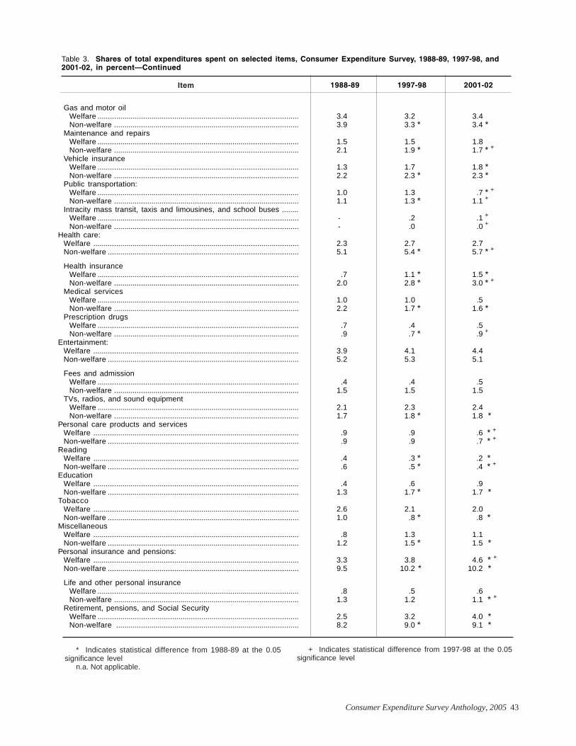
Consumer Expenditure Survey Anthology, 2005 43
Gas and motor oilWelfare ................................................................................................. 3.4 3.2 3.4Non-welfare ......................................................................................... 3.9 3.3 * 3.4 *
Maintenance and repairsWelfare ................................................................................................. 1.5 1.5 1.8Non-welfare ......................................................................................... 2.1 1.9 * 1.7 * +
Vehicle insuranceWelfare ................................................................................................. 1.3 1.7 1.8 *Non-welfare ......................................................................................... 2.2 2.3 * 2.3 *
Public transportation:Welfare ................................................................................................. 1.0 1.3 .7 * +
Non-welfare ......................................................................................... 1.1 1.3 * 1.1 +
Intracity mass transit, taxis and limousines, and school buses ........Welfare ................................................................................................. - .2 .1 +
Non-welfare ......................................................................................... - .0 .0 +
Health care:Welfare ................................................................................................... 2.3 2.7 2.7Non-welfare ............................................................................................ 5.1 5.4 * 5.7 * +
Health insuranceWelfare ................................................................................................. .7 1.1 * 1.5 *Non-welfare ......................................................................................... 2.0 2.8 * 3.0 * +
Medical servicesWelfare ................................................................................................. 1.0 1.0 .5Non-welfare ......................................................................................... 2.2 1.7 * 1.6 *
Prescription drugsWelfare ................................................................................................. .7 .4 .5Non-welfare ......................................................................................... .9 .7 * .9 +
Entertainment:Welfare ................................................................................................... 3.9 4.1 4.4Non-welfare ............................................................................................ 5.2 5.3 5.1
Fees and admissionWelfare ................................................................................................. .4 .4 .5Non-welfare ......................................................................................... 1.5 1.5 1.5
TVs, radios, and sound equipmentWelfare ................................................................................................. 2.1 2.3 2.4Non-welfare ......................................................................................... 1.7 1.8 * 1.8 *
Personal care products and servicesWelfare ................................................................................................... .9 .9 .6 * +
Non-welfare ............................................................................................ .9 .9 .7 * +
ReadingWelfare ................................................................................................... .4 .3 * .2 *Non-welfare ............................................................................................ .6 .5 * .4 * +
EducationWelfare ................................................................................................... .4 .6 .9Non-welfare ............................................................................................ 1.3 1.7 * 1.7 *
TobaccoWelfare ................................................................................................... 2.6 2.1 2.0Non-welfare ............................................................................................ 1.0 .8 * .8 *
MiscellaneousWelfare ................................................................................................... .8 1.3 1.1Non-welfare ............................................................................................ 1.2 1.5 * 1.5 *
Personal insurance and pensions:Welfare ................................................................................................... 3.3 3.8 4.6 * +
Non-welfare ............................................................................................ 9.5 10.2 * 10.2 *
Life and other personal insuranceWelfare ................................................................................................. .8 .5 .6Non-welfare ......................................................................................... 1.3 1.2 1.1 * +
Retirement, pensions, and Social SecurityWelfare ................................................................................................. 2.5 3.2 4.0 *Non-welfare ........................................................................................ 8.2 9.0 * 9.1 *
Table 3. Shares of total expenditures spent on selected items, Consumer Expenditure Survey, 1988-89, 1997-98, and2001-02, in percent—Continued
2001-021997-981988-89Item
* Indicates statistical difference from 1988-89 at the 0.05significance level
n.a. Not applicable.
+ Indicates statistical difference from 1997-98 at the 0.05significance level
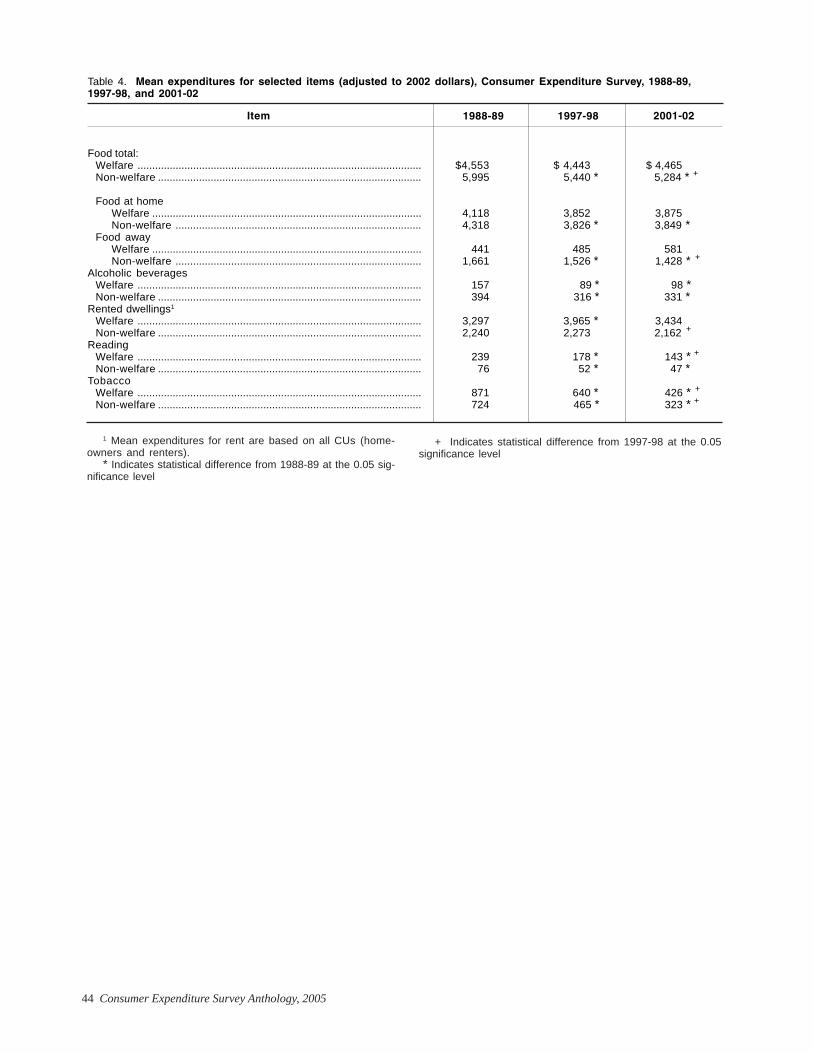
44 Consumer Expenditure Survey Anthology, 2005
Table 4. Mean expenditures for selected items (adjusted to 2002 dollars), Consumer Expenditure Survey, 1988-89,1997-98, and 2001-02
Food total:Welfare ................................................................................................. $4,553 $ 4,443 $ 4,465Non-welfare .......................................................................................... 5,995 5,440 * 5,284 * +
Food at homeWelfare ............................................................................................ 4,118 3,852 3,875Non-welfare .................................................................................... 4,318 3,826 * 3,849 *
Food awayWelfare ............................................................................................ 441 485 581Non-welfare .................................................................................... 1,661 1,526 * 1,428 * +
Alcoholic beveragesWelfare ................................................................................................. 157 89 * 98 *Non-welfare .......................................................................................... 394 316 * 331 *
Rented dwellings1
Welfare ................................................................................................. 3,297 3,965 * 3,434Non-welfare .......................................................................................... 2,240 2,273 2,162 +
ReadingWelfare ................................................................................................. 239 178 * 143 * +
Non-welfare .......................................................................................... 76 52 * 47 *Tobacco
Welfare ................................................................................................. 871 640 * 426 * +
Non-welfare .......................................................................................... 724 465 * 323 * +
1997-981988-89 2001-02Item
1 Mean expenditures for rent are based on all CUs (home-owners and renters).
* Indicates statistical difference from 1988-89 at the 0.05 sig-nificance level
+ Indicates statistical difference from 1997-98 at the 0.05significance level
Consumer Expenditure Survey Anthology, 2005 45
The growing population of olderAmericans has been an impor-tant focus of researchers and
policymakers for some time, with issuessuch as Social Security benefits, long-term care, and prescription drug costsat the forefront. Recent studies showthat an increasing number of these olderAmericans are also facing issues in-volved in raising children, such as therising costs of child care and highereducation. For example, the U.S. Cen-sus Bureau reports that, in 2000, ap-proximately 2.4 million grandparentswere “responsible for the basic needs”of their co-resident grandchildren.1 Atthe same time, the National Center forHealth Statistics reports that the num-ber of births to women aged 45-49 yearshas more than quadrupled since 1984,and births to women aged 50 and olderhave increased 13 percent annuallysince 1997.2 This article seeks to exam-ine the lifestyle and welfare of theseolder caregivers, using demographiccharacteristics and spending patternsderived from the Consumer ExpenditureSurvey (CE).
Spending Patterns ofOlder Consumers Raisinga Child
Abby Duly is an economist in the Branch ofInformation and Analysis, Division of Con-sumer Expenditure Surveys, Bureau of LaborStatistics.
Study methodologyData presented here were collected bythe CE Interview Survey during theyears 2000, 2001, and 2002. (Threeyears of data are necessary to providesufficient sample sizes for analysis.)The Interview component of the CE isused rather than the Diary because theInterview Survey is estimated to cover80 to 95 percent of total expendituresby consumer units (CUs).3 Specifically,the Interview Survey collects detaileddata on an estimated 60 to 70 percentof total household expenditures. Inaddition, global estimates, that is, ex-pense patterns for a 3-month period,are obtained for food and other se-lected items. These global estimatesaccount for an additional 20 to 25 per-cent of total expenditures.
The sample selected for this studyis divided into three groups, based pri-marily on the age of the reference per-son4 and the presence and age of chil-dren in the household. First, an “olderwith children” group is defined as hav-ing a reference person aged 60 or olderand at least one child under the age of18 years in the household. Furthermore,
ABBY DULY
1 Grandparents Living With Grandchil-dren: 2000. U.S. Census Bureau, October2003.
2 Martin J.A., Hamilton B.E., Sutton P.D.,Ventura S.J., Menacker F., Munson M.L.“Births: Final Data for 2002”, National Vi-tal Statistics Reports; Volume 52, Number 10.National Center for Health Statistics, 2003.
3 The Consumer Expenditure Survey col-lects data for consumer units. In this article,consumer units and households are used in-terchangeably. See the glossary at the end ofthis anthology for the definition of consumerunit.
4 See the glossary at the end of this an-thology for the definition of reference per-son.
46 Consumer Expenditure Survey Anthology, 2005
in order to ensure the role of the olderperson as caregiver, the sample is fur-ther restricted such that no other adultsreside in the home, except the spouseof the reference person, if there is one.Additionally, only the reference personand spouse may earn income. (Presum-ably, some working teenagers may con-tribute significantly to the householdbudget.5) Two other groups are se-lected for comparative purposes. First,in order to determine if there are gen-erational or age-related differencesamong households raising children, a“younger parents” group is selected,whose reference person is aged 35 to49 years and for whom there is at leastone child under the age of 18 years.Second, an “older without children”group, whose reference person is aged60 or older with no children present,provides a measure of how dependentchildren in the household may changethe lifestyle of the older generation.The additional criteria regarding otheradults and earners are also applied tothe younger parents and older withoutchildren groups for consistency. Fi-nally, all three sample groups containonly persons related by blood, mar-riage, adoption, or other legal arrange-ments. The resulting sample sizes are:9,869 younger parents; 18,056 CUs inthe older without children group; and206 older households with children.
The first part of the study is a com-parison of the three sample groups byselected demographic characteristics.Selected sample demographics are dis-played in table 1. Then, spending pat-terns are analyzed using expenditureshares, which are the proportions oftotal household expenditures allocatedto specific categories of expense.Shares analysis has two important ad-vantages in this study. First, using pro-portions of total spending allows formeaningful comparisons among groupsof CUs with very different incomes, asis the case here. (See table 1.) Addi-tionally, expenditure shares provideinsight into the relative importance ofone spending category over another,
indicating that some budgetary deci-sions are being made. In order to testthe significance of observed differ-ences in spending, the standard t-testformula is modified to account for theuse of proportional measures.6 Beforepresenting any findings, it is importantto note that the results of these analy-ses are not weighted to the generalpopulation.
Demographic comparisonsAs previously mentioned, the averageincomes of the three groups are quitedifferent. Most notable is the roughly$30,000-per-year gap between thoseolder CUs with children and those with-out children. Not surprisingly, thosewith children are younger on average(67 years old compared with 73 yearsold) and more likely to have an earnerin the household than their contempo-raries without children. It seems thathaving a child to raise may affect thedecision to retire or to obtain someemployment to supplement retirementincome. While almost two-thirds ofolder households without childrenhave a retired reference person, onlyabout 35 percent of older householdswith children are retirees. However, anadditional 11 percent of the latter havereference persons who are not work-ing for reasons other than retirement,including unemployment, disability,school attendance, or caring for thehome and/or family.
While the average income of oldercaregivers may more closely resemblethat of the younger parents group, edu-cational attainment appears to be moregenerational. The distribution of house-holds among educational levels are al-most identical between the two oldergroups, with the most prevalent cat-egory being high school graduate.Younger parents, on the other hand,are more likely to have reference per-sons who are college graduates (36percent of the sample) than any othereducational designation.
As shown in table 1, the sample con-tains different types of families. Forolder households without children,there are only two possible familytypes: 46 percent of these families aremarried couples, and 54 percent aresingle persons. Almost half of the oldercaregivers fall into the “other husbandand wife” category, which includesthose raising grandchildren or someother young relative, such as a nieceor nephew. When comparing two-parent households, those withyounger parents also are more likely tohave younger children. (Approximately12 percent have only children under theage of six, compared to just 1.5 percentof older households with children.) Forboth age groups, the majority of two-parent households have at least onechild, the oldest being between the agesof 6 and 17 years. There are a greaterpercentage of single parents in theyounger group (21 percent) than in theolder group (roughly 5 percent).
In terms of housing tenure, table 1shows that more than 75 percent ofeach of the groups studied are home-owners. However, while approximatelytwo-thirds of younger parents own ahome with a mortgage, 60 percent ofolder households without children and46 percent of older households withchildren own homes with no mortgage.
Other demographic comparisonsalso reveal differences among the threegroups of study. For example, the com-parisons by race and origin of the ref-erence person reveal that older care-givers are more likely to be Black andare more likely to be of Hispanic originthan either the younger parent groupor the older without children group.Finally, while younger parent house-holds and older households withoutchildren are similarly distributed acrossthe United States by region, a greaterpercentage of older caregivers live inthe South and West.
Analysis of expenditure sharesNot only is total annual spending dif-ferent, and actually higher, for olderhouseholds with children than eitherof the comparison groups, but the allo-cation of those dollars among selecteditem categories is also different. (See
5 See David S. Johnson and Mark Lino,“Teenagers: employment and contributionsto family spending,” Monthly Labor Review,September 2000, p. 15.
6 See Geoffrey Paulin, “Consumer expen-ditures on travel, 1980-87,” Monthly LaborReview, June 1990, p.60. See also GeoffreyPaulin, “The changing food-at-home budget:1980 and 1992 compared,” Monthly LaborReview, December 1998, p.32.
Consumer Expenditure Survey Anthology, 2005 47
table 2.) For example, older caregiversdevote a smaller proportion of total ex-penditures to food (9 percent) thanyounger parents and older householdswithout children, each of whom spendsroughly 13 percent. Examining the sub-components of the food category re-veals that the shares for both food athome and food away from home com-pare similarly to the category as a whole,although the differences are only sig-nificant7 for the proportions allocatedto food away from home. (The differ-ence in shares for food as a whole isalso significant between older house-holds with children and younger par-ents.)
Conversely to the food comparison,spending on housing accounts for agreater portion of the budget in house-holds with an older reference personand children (approximately 40 percent,compared with 33 percent for youngerparents and 29 percent for older house-holds without children). In the CE Sur-vey, the housing category is an aggre-gation of various subcategories. Forthis study, selected housing compo-nents are included either because theyare predominant in the total housingmeasure, such as shelter and utilities,or because they are particularly relevantto the analysis, such as child care andother domestic services. Shelter, whichincludes mortgage interest, propertytaxes, rent, and various expenses re-lated to the repair and maintenance ofa dwelling, is similar to the total hous-ing category, with older caregivers hav-ing the largest share of the three groupsstudied. Utility expenditures, on theother hand, make up a greater propor-tion of total spending by older house-holds without children than by thosewith children (approximately 8 percentcompared to 6 percent). Allocations oftotal spending to babysitting anddaycare are close between youngerparents and older households with chil-
dren at 1.9 percent and 1.2 percent, re-spectively. The same is true for otherdomestic services, for which olderhouseholds without children devote agreater proportion of total spending(roughly 6 percent) than younger par-ents and older caregivers, who eachdevote only one-half of 1 percent tothese services. (The category of “do-mestic services excluding child care”includes housekeeping services, gar-dening and lawn care, laundry and dry-cleaning, and care of the elderly or in-valid, among other services.)
Another category of expense inwhich the subcategories are particu-larly relevant to this study is apparel.As one might expect, the older with-out children group spends a signifi-cantly lesser share for all three subcat-egories of children’s clothing than theircontemporaries who have children inthe home. Younger parents, however,spend a significantly greater share foryoung girls’ and infants’ clothing thanthe older caregivers spend. The expen-diture shares for the apparel categoryas a whole are not significantly differ-ent among the groups, ranging fromabout 2.5 percent for older householdswithout children to 3.7 percent foryounger parents.
Perhaps, the most important spend-ing category analyzed here is healthcare. Spending on medical insurance,services, supplies, and prescriptiondrugs is a major budget concern forboth older Americans and families rais-ing children. In this study, age appearsto have the stronger positive effect onhealth care expenditures. Older house-holds without children, the group withthe highest average age, devote sig-nificantly greater shares of their totalspending to each component of healthcare than either of the other groups.In fact, the categorical shares ofyounger parents and older caregiversare almost identical, with the exceptionof prescription drugs, for which theshare allocated by younger parents issignificantly less.
Similar to health care, spending onpersonal insurance and pensions isalso related to age and employmentstatus. For example, retirees may no
longer make contributions to SocialSecurity or other pensions, and life in-surance premiums may cease beyonda certain age. So, it follows thatyounger parents, who are much morelikely to be working, allocate a signifi-cantly greater proportion of their totalspending to this category (roughly 11percent, compared with 5 percent byolder households without children and4 percent for older households withchildren).
One major expenditure category forwhich older caregivers spend signifi-cantly less, as a percentage of totalspending, than either of the compari-son groups is cash contributions.Older caregivers allocate just 3 percentto this category, which includes con-tributions to religious organizations,educational or other institutions, po-litical organizations, and cash supportfor college students, while older CUswithout children allocate more than 15percent of total expenditures. Youngerparents devote just less than 7 percentof their total budget to contributions.
There are no significant differencesin the allocations of total expendituresto transportation among the threetypes of households. The same is truefor entertainment shares, even whenspecifically examining purchases re-lated to children, such as pets, toys,and playground equipment. Althougholder households without children al-locate less than one-half of 1 percentof total expenditures to educationalexpenses, compared with 1.8 percentby older households with children and1.6 percent by younger parents, thedifferences are not statistically signifi-cant.
ConclusionThis article has presented sample de-mographic characteristics and spend-ing patterns for older CUs raising chil-dren. The results show that, for thesample studied, older caregivers aredifferent both from those in their gen-eration who have no children at homeand from younger parents. The demo-graphic comparison reveals that oldercaregivers are younger on average andearn roughly $30,000 more per year than
7 The t-test for significance is conductedin pairs–older with children compared to olderwithout children and older with children com-pared to younger parents–such that “signifi-cantly different” means “significantly dif-ferent from the older with children group.”
48 Consumer Expenditure Survey Anthology, 2005
older households without children.When compared with younger parents,older caregivers are less likely to havea college education and more likely toown their homes without a mortgage.Older households with children aremore likely to be Black and are morelikely to be of Hispanic origin than ei-ther of the comparison groups.
The expenditure share analysisshows that older caregivers andyounger parents allocate significantlydifferent percentages of total spend-ing to total food, food away from home,apparel for girls aged 2 to 15, apparelfor children under 2 years old, prescrip-tion drugs, personal insurance and pen-sions, and cash contributions. Differ-
ences in expenditure shares among theolder households with and withoutchildren are significant for food awayfrom home, babysitting and daycare,apparel for boys and girls aged 2 to 15,apparel for children under 2 years old,total health care, as well as all healthcare components, and cash contribu-tions.
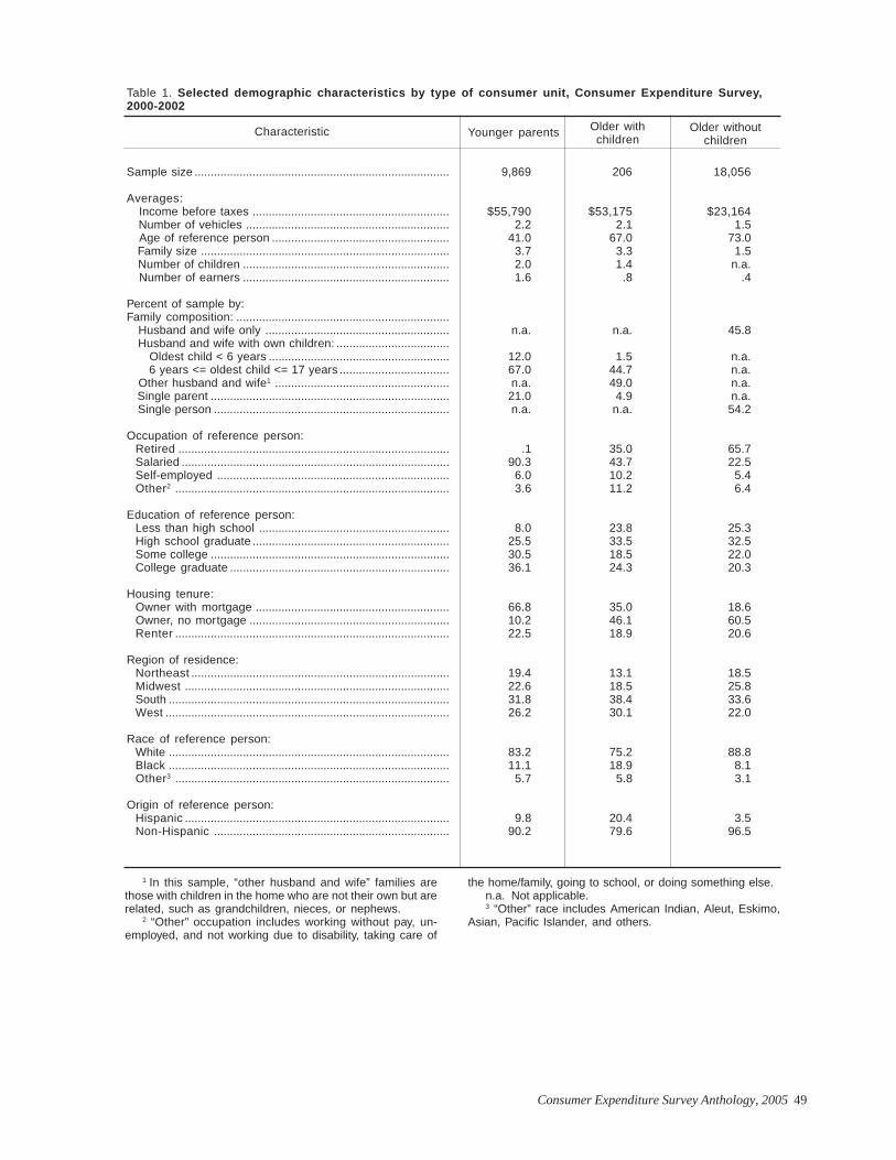
Consumer Expenditure Survey Anthology, 2005 49
Table 1. Selected demographic characteristics by type of consumer unit, Consumer Expenditure Survey,2000-2002
Younger parents
Sample size ............................................................................... 9,869 206 18,056
Averages: .................................................................................. Income before taxes ............................................................. $55,790 $53,175 $23,164 Number of vehicles ............................................................... 2.2 2.1 1.5 Age of reference person ....................................................... 41.0 67.0 73.0 Family size ............................................................................. 3.7 3.3 1.5 Number of children ................................................................ 2.0 1.4 n.a. Number of earners ................................................................ 1.6 .8 .4
Percent of sample by: ...............................................................Family composition: .................................................................. Husband and wife only ......................................................... n.a. n.a. 45.8 Husband and wife with own children: ................................... Oldest child < 6 years ........................................................ 12.0 1.5 n.a. 6 years <= oldest child <= 17 years .................................. 67.0 44.7 n.a. Other husband and wife1 ...................................................... n.a. 49.0 n.a. Single parent .......................................................................... 21.0 4.9 n.a. Single person ......................................................................... n.a. n.a. 54.2
Occupation of reference person:Retired .................................................................................... .1 35.0 65.7Salaried ................................................................................... 90.3 43.7 22.5Self-employed ........................................................................ 6.0 10.2 5.4Other2 ..................................................................................... 3.6 11.2 6.4
Education of reference person:Less than high school ........................................................... 8.0 23.8 25.3High school graduate ............................................................. 25.5 33.5 32.5Some college .......................................................................... 30.5 18.5 22.0College graduate .................................................................... 36.1 24.3 20.3
Housing tenure:Owner with mortgage ............................................................ 66.8 35.0 18.6Owner, no mortgage .............................................................. 10.2 46.1 60.5Renter ..................................................................................... 22.5 18.9 20.6
Region of residence:Northeast ................................................................................ 19.4 13.1 18.5Midwest .................................................................................. 22.6 18.5 25.8South ....................................................................................... 31.8 38.4 33.6West ........................................................................................ 26.2 30.1 22.0
Race of reference person:White ....................................................................................... 83.2 75.2 88.8Black ....................................................................................... 11.1 18.9 8.1Other3 ..................................................................................... 5.7 5.8 3.1
Origin of reference person:Hispanic .................................................................................. 9.8 20.4 3.5Non-Hispanic ......................................................................... 90.2 79.6 96.5
1 In this sample, “other husband and wife” families arethose with children in the home who are not their own but arerelated, such as grandchildren, nieces, or nephews.
2 “Other” occupation includes working without pay, un-employed, and not working due to disability, taking care of
Older withoutchildren
Older withchildren
the home/family, going to school, or doing something else.n.a. Not applicable.3 “Other” race includes American Indian, Aleut, Eskimo,
Asian, Pacific Islander, and others.
Characteristic
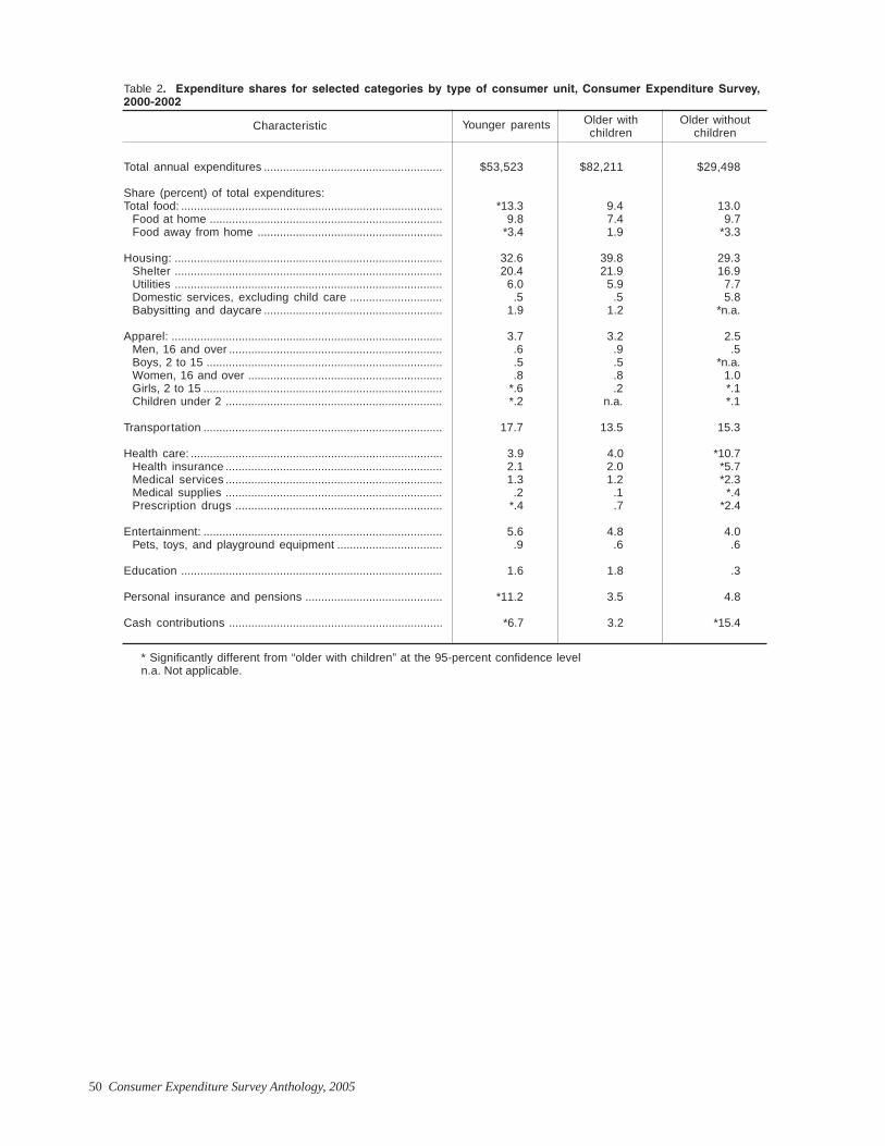
50 Consumer Expenditure Survey Anthology, 2005
Table 2. Expenditure shares for selected categories by type of consumer unit, Consumer Expenditure Survey,2000-2002
Total annual expenditures ........................................................ $53,523 $82,211 $29,498
Share (percent) of total expenditures: ....................................Total food: .................................................................................. *13.3 9.4 13.0
Food at home ......................................................................... 9.8 7.4 9.7Food away from home .......................................................... *3.4 1.9 *3.3
Housing: .................................................................................... 32.6 39.8 29.3Shelter .................................................................................... 20.4 21.9 16.9Utilities .................................................................................... 6.0 5.9 7.7Domestic services, excluding child care ............................. .5 .5 5.8Babysitting and daycare ........................................................ 1.9 1.2 *n.a.
Apparel: ..................................................................................... 3.7 3.2 2.5Men, 16 and over ................................................................... .6 .9 .5Boys, 2 to 15 .......................................................................... .5 .5 *n.a.Women, 16 and over ............................................................. .8 .8 1.0Girls, 2 to 15 ........................................................................... *.6 .2 *.1Children under 2 .................................................................... *.2 n.a. *.1
Transportation ........................................................................... 17.7 13.5 15.3
Health care: ............................................................................... 3.9 4.0 *10.7Health insurance .................................................................... 2.1 2.0 *5.7Medical services .................................................................... 1.3 1.2 *2.3Medical supplies .................................................................... .2 .1 *.4Prescription drugs ................................................................. *.4 .7 *2.4
Entertainment: ........................................................................... 5.6 4.8 4.0Pets, toys, and playground equipment ................................. .9 .6 .6
Education .................................................................................. 1.6 1.8 .3
Personal insurance and pensions ........................................... *11.2 3.5 4.8
Cash contributions ................................................................... *6.7 3.2 *15.4
* Significantly different from “older with children” at the 95-percent confidence leveln.a. Not applicable.
Older withoutchildren
Older withchildren
Younger parentsCharacteristic
Consumer Expenditure Survey Anthology, 2005 51
Tobacco Expenditures byEducation, Occupation,and Age
Mark Vendemia is an economist in theBranch of Information and Analysis, Divi-sion of Consumer Expenditure Surveys, Bu-reau of Labor Statistics.
MARK VENDEMIA Despite the heightened aware-ness of health problems asso-ciated with using tobacco
products, Americans continue to spendlarge amounts of money on these items.Data from the U.S. Bureau of Labor Sta-tistics (BLS or the Bureau) ConsumerExpenditure Survey (CE) show that, in2002, the average annual expenditureper consumer unit (CU)1 for tobaccoproducts and smoking supplies was$320. This is more than a 25 percentincrease over 1996, when the averageannual expenditure per CU on the sameitems was $255. (While the increase inexpenditures was more than 25 percent,it did not match the 106-percent rise inthe price of tobacco products andsmoking supplies, as measured by theBureau’s Consumer Price Index (CPI)during the same time period.)
MethodologyThis article looks at the amount spenton tobacco products and smoking sup-plies by CUs, as classified accordingto education, occupation, and age ofthe reference person. Tobacco prod-
ucts and smoking supplies consist ofthe following expenditure items: Ciga-rettes, other tobacco products, andsmoking accessories. In 2002, spend-ing on cigarettes accounted for 91 per-cent of expenditures on tobacco andsmoking supplies. Published expendi-ture estimates for cigarettes and othertobacco products are derived from datacollected in the CE’s Interview Survey,while estimates for smoking accesso-ries are derived from the Diary Survey.Because the expenditures collectedfrom the Diary Survey represent lessthan 1 percent of total tobacco spend-ing, percent reporting (the percent ofCUs who report purchasing an item) isbased on the Interview Survey only.In the Interview Survey, the mean ex-penditures are annualized figures,whereas the percent reportings are av-erage quarterly figures. Published CEexpenditure estimates for a particularitem are averages for all CUs in eachclass, including both those who pur-chase the item and those who do not.The mean for those who actually pur-chase the item is higher than the meanaveraged across purchasers and non-purchasers. For example, in 2002, theaverage expenditure for tobacco prod-ucts per CU was $320, while the aver-age for those who actually purchasedtobacco products was $1,321. This ar-ticle looks at mean expenditures for allCUs (purchasers and non-purchasers)and for CUs who reported purchasing
1 A consumer unit is defined as membersof a household related by blood, marriage,adoption, or other legal arrangement; a singleperson living alone or sharing a householdwith others but who is financially indepen-dent; or two or more persons living togetherwho share responsibility for at least two outof three major types of expenses—food,housing, and other expenses.
52 Consumer Expenditure Survey Anthology, 2005
tobacco. This paper focuses on the ra-tios of spending on tobacco, ratherthan the aggregate dollar amounts, be-cause of suspected underreporting forthis type of expenditure. For CUs whoreport tobacco expenditures, this analy-sis assumes consistent reporting (andunderreporting) levels across threedemographic groups—education, oc-cupation, and age.
Spending and share dataThis section examines tobacco expen-ditures, share allocation, and percentreporting, and compares tobacco ex-penditures with other selected expen-diture items classified by education,occupation, and age of the CU. To-bacco expenditures are compared withexpenditures for food and alcoholicbeverages to examine consumer spend-ing on necessary items, such as food,and on elective items, such as alcoholicbeverages. These ratios are based onaverage annual tobacco expenditures,as compared with average annual foodexpenditures and with average annualalcoholic beverage expenditures for allCUs within each group.
Education. In the CE Survey, educa-tion levels are divided into two majorcategories—less than college graduateand college graduate. Less than col-lege graduate is further subdivided intofour groups: Less than high schoolgraduate, high school graduate, highschool graduate with some college, andassociate degree. College graduate issubdivided into two groups: bachelor’sdegrees and master’s, professional, ordoctoral degrees. For those CUs whosereference persons had less than a col-lege degree, the average annual expen-diture for tobacco was $375 in 2002.(See table 1.) In contrast, the averageannual tobacco expenditure for thoseCUs whose reference person had a col-lege degree was nearly half at $167.High school graduates had the high-est average annual tobacco expendi-ture at $441, while those with a master’s,professional, or doctoral degree hadthe lowest at $130—a difference of 239percent.
When comparing all CUs (bothhouseholds that do and do not report
tobacco expenditures), there is lessvariation in the average annual tobaccoexpenditures among the different edu-cation levels when the analysis is re-stricted to those consumers who actu-ally reported tobacco expenditures.The average annual tobacco expendi-ture for those who reported such ex-penditures was $1,321 per year, with thehighest average for the high schoolgroup at $1,453 and the lowest averagefor the bachelor’s degree group at$1,161— a 25-percent difference.
Less than 1 percent of total averageannual CU expenditures was spent ontobacco in 2002. The percent share ofthe average annual amount spent ontobacco varies among those house-holds with less than a college degree.For those households with less than ahigh school degree, the tobacco shareof average annual expenditures was 1.4percent, compared with 1.3 percent forthose with a high school degree, 0.9percent for high school graduates withsome college, and 0.7 percent for thosehouseholds with an associate degree.The share spent on tobacco was lowerfor those households with a collegedegree—0.4 percent for those with abachelor’s degree and 0.2 percent forthose with a master’s, professional, ordoctoral degree. On average, whenlooking at all CUs, including those CUsnot reporting tobacco expenditures, asCUs achieve higher levels of education,the share that they spend on tobaccobecomes smaller. However, as noted inthe previous paragraph, the differencesin average annual tobacco expendituresby CUs who reported tobacco expen-ditures show less variation among edu-cation levels.
Twenty-four percent of CUs re-ported tobacco expenditures in 2002.Thirty percent of high school gradu-ates with no college—the highest ofall educational groups—reported mak-ing tobacco purchases, followed by thegroup with less than a high school de-gree and those high school graduateswith some college, both at 27 percent,and the group with an associate de-gree at 24 percent. On the other hand,fewer college graduates reported to-bacco purchases with 16 percent of
those CUs with a bachelor’s degree and10 percent of those with a master’s, pro-fessional, or doctoral degree reportingsuch expenditures.
The amount spent on tobacco com-pared with the amount spent on foodand alcohol is also interesting. Over-all, for all CUs, the amount spent ontobacco averaged about 6 percent ofthat spent on food; but for those witha high school degree, the amount was9 percent, whereas it was only 2 per-cent for those with a master’s, profes-sional, or doctoral degree. The amountspent on tobacco averaged about 85percent of that spent on alcoholic bev-erages for all CUs. For those with lessthan a high school degree, the amountwas 191 percent; for those with an as-sociate degree, the amount was 67 per-cent; and for those with a master’s, pro-fessional, or doctoral degree, theamount was only 22 percent. (See table2.)
Households with less than a collegedegree made up 74 percent (this group’spopulation share) of all CUs but ac-counted for 86 percent of total tobaccoexpenditures in 2002, while those witha college degree made up 26 percent ofall CUs but accounted for only 14 per-cent of tobacco expenditures.
Occupation. CE Survey data are pub-lished for the following occupationgroups: Self-employed workers; CUswith retired reference persons; wageand salary earners, which includes fiveoccupation groups—managers andprofessionals; technical, sales, andclerical workers; service workers; con-struction workers and mechanics; andoperators, fabricators and laborers—and all others, including those not re-porting. CUs with retired reference per-sons had the lowest average annualtobacco expenditures at $163. The twomore traditional blue-collar occupationgroups, construction workers and me-chanics, and operators, fabricators,and laborers, had the highest averageannual tobacco expenditures at $582and $482, respectively. In comparison,managers and professionals spent$251, and self-employed workers spent$315.
Consumer Expenditure Survey Anthology, 2005 53
There is less variation in averageannual tobacco expenditures amongoccupation groups for those CUs whoreported tobacco expenditures, whencompared with the average for all CUsin the demographic group. The aver-age annual tobacco expenditure forthose who reported tobacco expendi-tures was $1,321 per year, with the high-est average expenditure for the con-struction workers and mechanics groupat $1,464 and the lowest for the retiredgroup at $1,189.
The percent share of the averageannual amount spent on tobacco alsovaries greatly among occupationgroups. Managers’ and professionals’share of average annual tobacco ex-penditures was 0.4 percent, comparedwith 0.6 percent for CUs with retiredreference persons, and 0.7 percent forself-employed workers. The share washigher for the more traditional blue-collar households, with a share of 1.1percent for service workers, and 1.4 per-cent for both construction workers andmechanics, and operators, fabricators,and laborers.
Forty percent of the constructionworkers and mechanics group—thehighest of all occupational groups—reported tobacco expenditures in 2002,followed closely by operators, fabrica-tors, and laborers at 35 percent, andservice workers at 30 percent. In con-trast, 19 percent of managers and pro-fessionals and 14 percent of the retiredgroup reported tobacco expenditures.
As noted above, for all CUs, theamount spent on tobacco averaged 6percent of that spent on food; but forconstruction workers and mechanics,the amount was 11 percent, comparedwith only 4 percent for managers andprofessionals, as well as CUs with re-tired reference persons. The amountspent on tobacco averaged 137 percentof that spent on alcoholic beveragesfor operators, fabricators, and laborers,compared with 117 percent for serviceworkers, 63 percent for self-employedworkers, and only 45 percent for man-agers and professionals.
In 2002, the households of manag-ers and professionals made up 24 per-cent of CUs but accounted for 19 per-
cent of total tobacco expenditures. Thehouseholds with retired reference per-sons made up 17 percent of all CUs andaccounted for 9 percent of tobacco ex-penditures. In contrast, the house-holds of construction workers and me-chanics, and operators, fabricators,and laborers made up 4 percent and 10percent of all CUs, respectively, but ac-counted for 8 percent and 15 percentof tobacco expenditures.
Age. The CE Survey publishes datafor the following age classes: Underthe age of 25, 25 to 34 years, 35 to 44years, 45 to 54 years, age 65 and over,65 to 74 years, and age 75 and over.Households headed by someone 45 to54 years of age had the highest aver-age annual tobacco expenditure at $415,whereas the 75-and-over householdshad the lowest at $81—a difference of412 percent. In comparison, the aver-age annual tobacco expenditure for theunder-25 group was $286, comparedwith $376 for the 35-to-44 age group,and $220 for the 65-to-74 age group.
There is less variation in averageannual tobacco expenditures amongage groups for those CUs who reportedtobacco expenditures when comparedto the average annual expenditures forall CUs (including those who did notreport having tobacco expenditures).The group with the highest averageexpenditure was the 45-to-54 age groupat $1,413, and the group with the low-est was the under-25 group at $1,100—a 28 percent difference.
For the 75-and-older group, theshare of average annual expendituresfor tobacco was 0.3 percent, comparedwith 0.5 percent for the 65-and-oldergroup, and 0.8 percent for the 25-to-34,35-to-44, and 55-to-64 age groups. Theshare of average annual expenditureson tobacco was highest for the young-est households, with a share of 1.2 per-cent for the under-25 group.
As previously mentioned, 24 percentof all CUs reported tobacco expendituresin 2002. Twenty-nine percent of the 45-to-54 group—the highest of all agegroups—reported tobacco expendi-tures, followed closely by the 35-to-44age group at 27 percent and by the 25-
to-34, 55-to-64, and under-25 age groupsat 26 percent. In contrast, only 12 per-cent of the 65-and-over age group, 17percent of the 65-to-74 age group, and 7percent of the 75-and-over age groupreported tobacco expenditures.
A comparison of the amount spenton tobacco with the amount spent onfood shows that, for the under-25group—the highest of all age groups—the amount spent on tobacco was 8percent, compared with only 3 percentfor the 75-and-over group. The amountspent on tobacco averaged 103 percentof that spent on alcoholic beveragesfor the 35-to-44 group, 89 percent forthe 45-to-54 group, 80 percent for the25-to-34 group, 73 percent for the un-der-25 group, 68 percent for the 65-to-74 group, and 56 percent for the 75-and-over group.
In 2002, households headed bysomeone aged 65 and over made up 20percent of CUs but accounted for only9 percent of total tobacco expenditures,whereas those households headed bysomeone under 25 years old made up8 percent of all CUs and accounted for7 percent of tobacco expenditures. Incontrast, the 35- to 44-year-old groupand the 45- to 54-year-old group madeup 22 percent and 20 percent of all CUs,respectively, but accounted for 26 per-cent of the tobacco expenditures.
In summary, CE 2002 data showsthat, as CUs achieve higher levels ofeducation, the amounts and shares thatthey spend on tobacco becomessmaller. Among occupation groups (ex-cluding retired households), house-holds of managers and professionalsand self-employed workers spend asmaller amount and have the lowestshare of tobacco expenditures. Con-struction workers and mechanics aswell as operators, fabricators, and la-borers spend a larger amount and shareon tobacco. As age increases amonggroups, the amounts and the sharesthat they spend on tobacco becomessmaller. While the percent of CUs whopurchase tobacco differs by age, edu-cation, and occupation, the averageannual expenditure on tobacco by CUswho purchase tobacco does not differas widely by these factors.
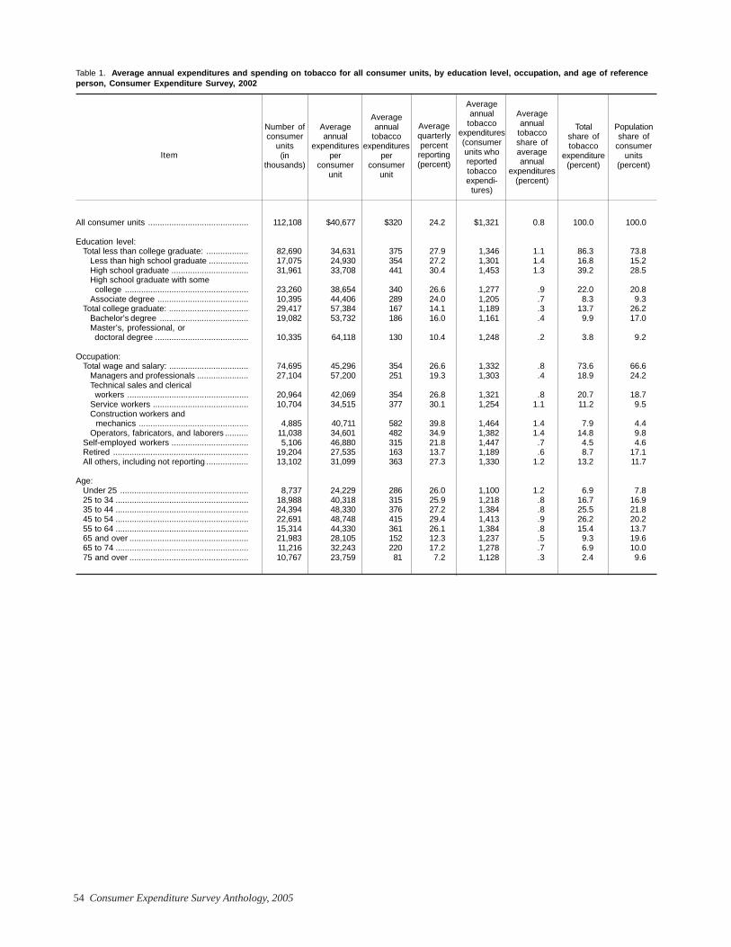
54 Consumer Expenditure Survey Anthology, 2005
Table 1. Average annual expenditures and spending on tobacco for all consumer units, by education level, occupation, and age of referenceperson, Consumer Expenditure Survey, 2002
All consumer units ........................................... 112,108 $40,677 $320 24.2 $1,321 0.8 100.0 100.0
Education level:Total less than college graduate: .................. 82,690 34,631 375 27.9 1,346 1.1 86.3 73.8
Less than high school graduate ................. 17,075 24,930 354 27.2 1,301 1.4 16.8 15.2High school graduate ................................. 31,961 33,708 441 30.4 1,453 1.3 39.2 28.5High school graduate with some college ..................................................... 23,260 38,654 340 26.6 1,277 .9 22.0 20.8Associate degree ....................................... 10,395 44,406 289 24.0 1,205 .7 8.3 9.3
Total college graduate: .................................. 29,417 57,384 167 14.1 1,189 .3 13.7 26.2Bachelor’s degree ...................................... 19,082 53,732 186 16.0 1,161 .4 9.9 17.0Master’s, professional, or doctoral degree ........................................ 10,335 64,118 130 10.4 1,248 .2 3.8 9.2
Occupation:Total wage and salary: .................................. 74,695 45,296 354 26.6 1,332 .8 73.6 66.6
Managers and professionals ...................... 27,104 57,200 251 19.3 1,303 .4 18.9 24.2Technical sales and clerical workers .................................................... 20,964 42,069 354 26.8 1,321 .8 20.7 18.7Service workers ......................................... 10,704 34,515 377 30.1 1,254 1.1 11.2 9.5Construction workers and mechanics ............................................... 4,885 40,711 582 39.8 1,464 1.4 7.9 4.4Operators, fabricators, and laborers .......... 11,038 34,601 482 34.9 1,382 1.4 14.8 9.8
Self-employed workers ................................. 5,106 46,880 315 21.8 1,447 .7 4.5 4.6Retired .......................................................... 19,204 27,535 163 13.7 1,189 .6 8.7 17.1All others, including not reporting .................. 13,102 31,099 363 27.3 1,330 1.2 13.2 11.7
Age:Under 25 ....................................................... 8,737 24,229 286 26.0 1,100 1.2 6.9 7.825 to 34 ......................................................... 18,988 40,318 315 25.9 1,218 .8 16.7 16.935 to 44 ......................................................... 24,394 48,330 376 27.2 1,384 .8 25.5 21.845 to 54 ......................................................... 22,691 48,748 415 29.4 1,413 .9 26.2 20.255 to 64 ......................................................... 15,314 44,330 361 26.1 1,384 .8 15.4 13.765 and over ................................................... 21,983 28,105 152 12.3 1,237 .5 9.3 19.665 to 74 ......................................................... 11,216 32,243 220 17.2 1,278 .7 6.9 10.075 and over ................................................... 10,767 23,759 81 7.2 1,128 .3 2.4 9.6
Averagequarterlypercentreporting(percent)
Averageannual
tobaccoexpenditures(consumerunits whoreportedtobaccoexpendi-
tures)
Averageannual
tobaccoshare ofaverageannual
expenditures(percent)
Totalshare oftobacco
expenditure(percent)
Populationshare of
consumerunits
(percent)Item
Number ofconsumer
units(in
thousands)
Averageannual
expendituresper
consumerunit
Averageannual
tobaccoexpenditures
perconsumer
unit
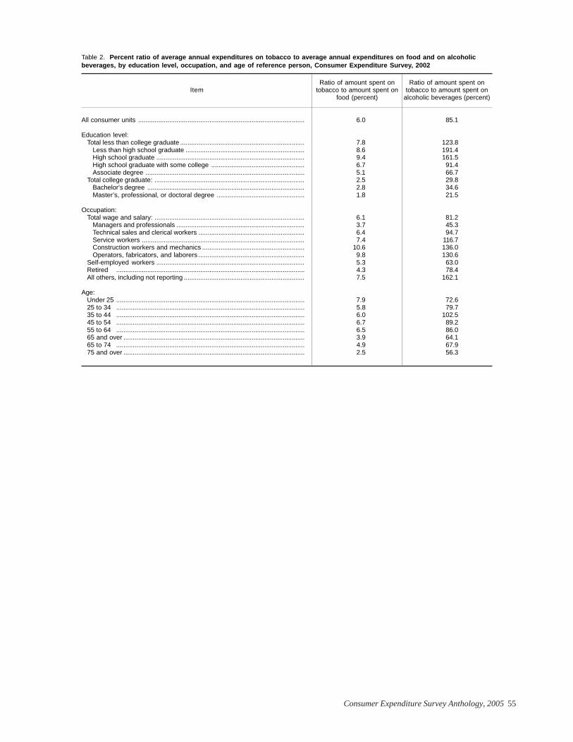
Consumer Expenditure Survey Anthology, 2005 55
Table 2. Percent ratio of average annual expenditures on tobacco to average annual expenditures on food and on alcoholicbeverages, by education level, occupation, and age of reference person, Consumer Expenditure Survey, 2002
All consumer units ........................................................................................... 6.0 85.1
Education level:Total less than college graduate .................................................................... 7.8 123.8
Less than high school graduate ................................................................. 8.6 191.4High school graduate ................................................................................. 9.4 161.5High school graduate with some college ................................................... 6.7 91.4Associate degree ....................................................................................... 5.1 66.7
Total college graduate: .................................................................................. 2.5 29.8Bachelor’s degree ...................................................................................... 2.8 34.6Master’s, professional, or doctoral degree ................................................ 1.8 21.5
Occupation:Total wage and salary: .................................................................................. 6.1 81.2
Managers and professionals ...................................................................... 3.7 45.3Technical sales and clerical workers .......................................................... 6.4 94.7Service workers ......................................................................................... 7.4 116.7Construction workers and mechanics ........................................................ 10.6 136.0Operators, fabricators, and laborers .......................................................... 9.8 130.6
Self-employed workers ................................................................................. 5.3 63.0Retired ....................................................................................................... 4.3 78.4All others, including not reporting .................................................................. 7.5 162.1
Age:Under 25 ....................................................................................................... 7.9 72.625 to 34 ....................................................................................................... 5.8 79.735 to 44 ....................................................................................................... 6.0 102.545 to 54 ....................................................................................................... 6.7 89.255 to 64 ....................................................................................................... 6.5 86.065 and over ................................................................................................... 3.9 64.165 to 74 ....................................................................................................... 4.9 67.975 and over ................................................................................................... 2.5 56.3
ItemRatio of amount spent on
tobacco to amount spent onfood (percent)
Ratio of amount spent ontobacco to amount spent on
alcoholic beverages (percent)
56 Consumer Expenditure Survey Anthology, 2005
Spending by Singles
Meaghan Duetsch is an economist in theBranch of Information and Analysis, Divi-sion of Consumer Expenditure Surveys, Bu-reau of Labor Statistics.
MEAGHAN DUETSCH Do single women spend theirmoney differently than singlemen do? If so, can their spend-
ing differences be attributed to differ-ences in characteristics between thetwo groups? In addition, have thespending patterns of single men andsingle women changed over the pastdecade? These are some of the ques-tions that can be answered with datafrom the Consumer Expenditure Survey.Given that people are choosing to marryat a later age and that the life expect-ancy of women continues to be greaterthan that of men, more people are singlenow than ever before, so the answersto the preceding questions loom largein the economic life of a significant pro-portion of the Nation’s population.
This article examines the expendi-tures of single-person consumer units,both men and women. A single-personconsumer unit may differ slightly froma single-person, or one-person, house-hold. Financial independence is a cri-terion used to determine consumer unitstatus. A one-person household is asingle-person consumer unit; but if twopeople are living together and are fi-nancially independent of one another,as in a roommate situation, then the twopeople are two separate single-personconsumer units. Single parents withchildren present are not single-personconsumer units. Using data for 1991–92 and 2001–02 from the interview and
diary portions of this Consumer Ex-penditure Survey, this article com-pares expenditures and demographiccharacteristics between and duringthose two periods. Two years of dataare used for each period, in order toobtain a sufficient sample for examin-ing expenditures by age and gender.Only single men and single women arecompared, as opposed to all men andall women, due to the way data are col-lected. The Consumer Expenditure Sur-vey collects data on expenditures forthe consumer unit as a whole, with nodistinction as to who made the expen-ditures. Therefore, in a consumer unitof more than one person, it cannot bedetermined who made the expenditures,whereas that is not the case in a single-person consumer unit. Expenditures areexamined to determine whether theychanged for each gender over the pe-riod from 1991–92 through 2001–02 andalso to determine whether the expendi-ture relationship between genderschanged during that time. Finally, ex-penditures are examined for a specificage group, to analyze the role of age inexpenditure decisions.
CharacteristicsThe average age of single women wasabout 13 years older than the averageage for single men for the 1991–92 pe-riod (56.6 years and 43 years, respec-tively) and about 11 years older for the
Consumer Expenditure Survey Anthology, 2005 57
2001–02 period (56.3 years and 45.3years, respectively). (See table 1.) Sincemen and women’s birthrates are ap-proximately equal and women have alonger life expectancy, there are moreolder women than older men. This dif-ference could also explain the higherhomeownership rates for single women,48 percent in 1991–92, compared with36 percent for single men. Both groupshad increased homeownership rates in2001–02, with women at 56 percent andmen at 45 percent. Across the two peri-ods, more female homeowners werewithout a mortgage than with, a statis-tic again most likely attributable to thelongevity of women, which results inmany older widows. Male homeownerswere fairly evenly split between thosewith a mortgage and those without, andthis ratio stayed constant over the twoperiods, despite an increase in men’shomeownership. Both groups experi-enced an increase in the percentagewith a college education: in 1991–92,46 percent of single women and 54 per-cent of single men had a college edu-cation—figures that increased to 54percent for single women and 61 per-cent for single men in 2001–02.
Single men had higher average in-comes than did single women for both1991–92 and 2001–02, and the differ-ence increased over the period. Men’sincome grew from $20,615 to $31,688,(an increase of 54 percent), whilewomen’s rose from $16,432 to $22,930(an increase of 40 percent). Althoughsingle men still owned more vehiclesthan did single women, the men’s rateof ownership remained constant. Onaverage, men had 1.3 vehicles in bothperiods, while women had 0.8 vehiclesin 1991–92 and 0.9 in 2001–02.
ExpendituresSingle men and single women allocatetheir expenditures differently. Expendi-ture patterns were examined by look-ing at shares of total expenditures, be-cause nominal dollar amounts of theexpenditures, as well as the nominalamount of average annual expenditures,change over time. The difference inshares held for both periods. Singlemen spent a larger share of annual ex-
penditures on food than did singlewomen (13.5 percent as opposed to 12.6percent in 1991–92, and 12.5 percentcompared with 11.6 percent in 2001–02). The genders also allocated theirspending differently between food athome and food away from home, withmen apportioning a larger share of theirfood dollar to food away from homeand women a larger share to food athome. This distinction may be ex-plained by the fact that single womenas a group are older than single menand, therefore, take more meals at home.Also, traditionally, women cook morethan men. In addition, only about halfof all single women are earners. (Seetable 1.) This fact may contribute towomen allocating a larger share of ex-penditures to food at home, becausefood at home is usually less expensive.Single women spent a larger share oftheir expenditures on housing than didsingle men (38 percent and 33 percent,respectively). The reason could be thehigher homeownership rate for singlewomen, or it may be that single womenhad lower incomes and, thus, spent alarger proportion on necessities. Singlewomen allocated a larger share to ap-parel and services, while single menallocated a larger share to transporta-tion. This larger share that men allo-cated to transportation is attributed tothe higher average number of vehiclesowned by men, together with the asso-ciated costs, such as gasoline, mainte-nance, and insurance. Single women al-located a larger share to health care,compared with single men, while singlemen spent a larger share of annual ex-penditures on entertainment than didsingle women. Both groups spentabout the same share on cash contri-butions.
There were several similarities in thetrends of expenditure shares for menand women between 1991–92 and2001–02. Over the 10-year interval, eachgroup decreased its share spent onfood, including food at home and foodaway from home. The shares allocatedfor housing, shelter, and utilities re-mained relatively constant. Bothgroups spent a smaller share on apparelin 2001–02 than in 1991–92. By con-
trast, both groups allocated a largershare to transportation in 2001–02 thanin 1991–92. The expenditure sharespent on health care rose slightly forboth men and women, while the sharesspent on entertainment and cash con-tributions remained relatively un-changed.
The preceding discussion of singlemen and single women encompassesall singles, ranging from young adultsto those who have reached retirementage and beyond. Many differences inthe spending patterns described canbe attributed to the average differencein age between single men and singlewomen. The analysis that follows com-pares income levels and spending pat-terns between men and women in aspecific age group to see if the spend-ing differences between the gendersremain for men and women of a similarage. The 25- to 34-year-old age groupis examined because it represents thoseoften thought of when the word“singles” is used. The men and womenof this group have similarities and dif-ferences. In 1991–92, single women andsingle men had similar average incomes($24,721 and $24,719, respectively) andsimilar average annual expenditures($21,312 and $21,858, respectively).However, in that same period, thesingle men allocated a larger share tofood (13.4 percent compared with 11.8percent), but both the men and thewomen allocated about the same shareto food at home (5.6 percent and 5.2percent, respectively). (See table 2.)Single men allocated a larger share tofood away from home (7.7 percent asopposed to 6.6 percent). Single womenin this group allocated a slightly largershare to housing overall (36.4 percentcompared with 34.2 percent) and alsoallocated a slightly larger share to shel-ter (25.4 percent versus 23.8 percent).By contrast, and unlike the situationfor all age groups taken together, singlewomen aged 25 to 34 years had a lowerhomeownership rate (17 percent) thandid single men (24 percent). Women andmen in the group allocated about thesame share to utilities (5.6 percent and5.4 percent, respectively), even thoughthe women were a higher percentage
58 Consumer Expenditure Survey Anthology, 2005
SummarySingle women overall are older thansingle men and have higher rates ofhomeownership. Single men have alarger number of vehicles. However,both groups had an increase in the rateof homeownership from 1991–92 to2001–02. Both groups also had an in-crease in the number of college edu-cated among them from the first periodto the second. Both single men andsingle women spent less of their totalexpenditures in 2001–02 on food andapparel and services, although menspent more on food and women moreon apparel and services. As incomesincrease, people tend to spend less onnecessities, such as food. Also, thedecrease in the costs of apparel andservices relative to other goods,coupled with increasing incomes,across the two periods, has enabledconsumers to allocate less of their to-tal expenditures to apparel and ser-vices. Single men and single womenaged 25 to 34 years exhibited spend-ing patterns more similar to each otherthan did the overall groups of single menand single women. The 25- to 34-year-old men and women had similar ratesof homeownership and similar levelsof education and also spent similarlyon shelter, as well as on entertainment.However, single men spent more ontransportation and single women moreon apparel and services. Overall, singlemen and single women had differentspending patterns that changed littlefrom 1991–92 to 2001–02.
of renters (83 percent) than were themen (76 percent). (Because utilities areoften included in rent payments, it isnot possible to capture the true expen-diture for utilities by renters.) Singlewomen aged 25 to 34 years allocated alarger share to apparel and services (7.6percent) than did single men in the sameage group (4.5 percent). In the 1991–92period, the 25- to 34-year-old men spenta larger share on transportation (17.9percent) than did the 25- to 34-year-oldwomen (15.7 percent). Men had an av-erage of 1.4 vehicles; women an aver-age of 0.9 vehicles. Also in 1991–92,single women allocated a larger shareto health care (3.1 percent) than didsingle men (2.1 percent). However,single men spent a larger share (2.5percent) on cash contributions than didsingle women (0.9 percent).
The picture for singles 25 to 34years old changed some by 2001–02.In that period, single men had averageincomes of $38,936 and average annualexpenditures of $29,736, while singlewomen had lower incomes ($31,432)and lower average annual expenditures($27,110). Also in 2001–02, 90 percent ofsingle women were earners, comparedwith 100 percent of single men. Thehomeownership rate increased overthe1991–92 figures for both men andwomen, to 33 percent and 30 percent,respectively. Also, more women in thisage group had a college education (80percent) than did men (75 percent), al-though the differences between thegroups were narrower than in 1991–92
(77 percent of women and 70 percent ofmen).
Although there were some differ-ences from the 1991–92 period, in 2001–02 single men still allocated a largershare to food (12.9 percent) than didsingle women (11.8 percent), as well asa larger share to food away from home(8.8 percent compared with 6.0 percent).Single women still allocated a largershare to housing overall (37.7 percentas opposed to 33.7 percent), eventhough a larger percentage of 25- to34-year-old single men were home-owners. In addition, single women al-located a larger share to shelter (25.9percent) than did single men (23.8 per-cent). In 2001–02, the share allocatedto apparel and services by all singles25 to 34 years decreased from the 1991–92 figure; however, the share spent bysingle women decreased more, to 5.7percent, compared with single men’sshare of 4.1 percent. As in the 1991–92period, 25- to 34-year-old single menspent a larger share on transportation(20.4 percent) than did single women(17.7 percent) in 2001–02. Single menhad slightly fewer vehicles, 1.2, com-pared with 1.4 vehicles in 1991–92;single women had 1.0 and 0.9 in therespective periods. Single men contin-ued to allocate a larger share—morethan twice as much—to cash contribu-tions (2.9 percent) than did singlewomen (1.4 percent), possibly due tochild support payments that single menmake, as they may be fathers of youngchildren who live elsewhere.
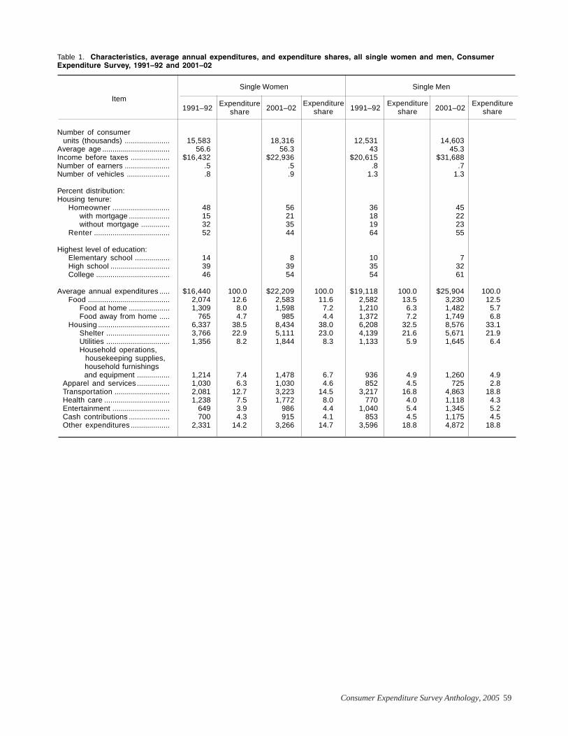
Consumer Expenditure Survey Anthology, 2005 59
Table 1. Characteristics, average annual expenditures, and expenditure shares, all single women and men, ConsumerExpenditure Survey, 1991–92 and 2001–02
Number of consumer units (thousands) ...................... 15,583 18,316 12,531 14,603Average age ................................. 56.6 56.3 43 45.3Income before taxes ................... $16,432 $22,936 $20,615 $31,688Number of earners ...................... .5 .5 .8 .7Number of vehicles ..................... .8 .9 1.3 1.3
Percent distribution:Housing tenure:
Homeowner ............................ 48 56 36 45with mortgage .................... 15 21 18 22without mortgage .............. 32 35 19 23
Renter ..................................... 52 44 64 55
Highest level of education:Elementary school ................. 14 8 10 7High school ............................. 39 39 35 32College .................................... 46 54 54 61
Average annual expenditures ..... $16,440 100.0 $22,209 100.0 $19,118 100.0 $25,904 100.0Food ........................................ 2,074 12.6 2,583 11.6 2,582 13.5 3,230 12.5
Food at home .................... 1,309 8.0 1,598 7.2 1,210 6.3 1,482 5.7Food away from home ..... 765 4.7 985 4.4 1,372 7.2 1,749 6.8
Housing ................................... 6,337 38.5 8,434 38.0 6,208 32.5 8,576 33.1Shelter ............................... 3,766 22.9 5,111 23.0 4,139 21.6 5,671 21.9Utilities ............................... 1,356 8.2 1,844 8.3 1,133 5.9 1,645 6.4Household operations, housekeeping supplies, household furnishings and equipment ................ 1,214 7.4 1,478 6.7 936 4.9 1,260 4.9
Apparel and services ................ 1,030 6.3 1,030 4.6 852 4.5 725 2.8Transportation ........................... 2,081 12.7 3,223 14.5 3,217 16.8 4,863 18.8Health care ................................ 1,238 7.5 1,772 8.0 770 4.0 1,118 4.3Entertainment ............................ 649 3.9 986 4.4 1,040 5.4 1,345 5.2Cash contributions .................... 700 4.3 915 4.1 853 4.5 1,175 4.5Other expenditures ................... 2,331 14.2 3,266 14.7 3,596 18.8 4,872 18.8
Single Women Single Men
Item1991–92
Expenditureshare
Expenditureshare
Expenditureshare
Expenditureshare 2001–021991–922001–02
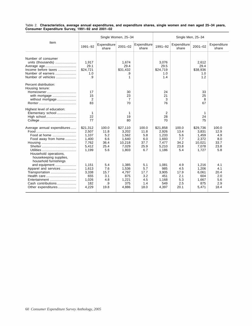
60 Consumer Expenditure Survey Anthology, 2005
Table 2. Characteristics, average annual expenditures, and expenditure shares, single women and men aged 25–34 years,Consumer Expenditure Survey, 1991–92 and 2001–02
Number of consumer units (thousands) ....................... 1,917 1,674 3,076 2,612Average age .................................. 29.1 29.4 29.5 29.4Income before taxes .................... $24,721 $31,432 $24,719 $38,936Number of earners ....................... 1.0 .9 1.0 1.0Number of vehicles ...................... .9 1 1.4 1.2
Percent distribution:Housing tenure:
Homeowner ................................ 17 30 24 33with mortgage .......................... 15 23 21 25without mortgage ..................... 2 7 3 8
Renter ......................................... 83 70 76 67
Highest level of education:Elementary school ..................... 1 1 2 1High school ................................. 22 19 28 24College ........................................ 77 80 70 75
Average annual expenditures ...... $21,312 100.0 $27,110 100.0 $21,858 100.0 $29,736 100.0Food ............................................ 2,507 11.8 3,202 11.8 2,926 13.4 3,831 12.9
Food at home .......................... 1,107 5.2 1,562 5.8 1,233 5.6 1,459 4.9Food away from home ............ 1,400 6.6 1,640 6.0 1,693 7.7 2,372 8.0
Housing ...................................... 7,762 36.4 10,218 37.7 7,477 34.2 10,021 33.7Shelter ...................................... 5,412 25.4 7,029 25.9 5,210 23.8 7,078 23.8Utilities ...................................... 1,199 5.6 1,803 6.7 1,186 5.4 1,727 5.8Household operations,
housekeeping supplies, household furnishings and equipment ....................... 1,151 5.4 1,385 5.1 1,081 4.9 1,216 4.1
Apparel and services ................. 1,613 7.6 1,536 5.7 985 4.5 1,206 4.1Transportation ............................ 3,338 15.7 4,797 17.7 3,905 17.9 6,061 20.4Health care ................................. 655 3.1 875 3.2 451 2.1 604 2.0Entertainment ............................. 1,026 4.8 1,221 4.5 1,168 5.3 1,667 5.6Cash contributions ..................... 182 .9 375 1.4 549 2.5 875 2.9Other expenditures .................... 4,229 19.8 4,886 18.0 4,397 20.1 5,471 18.4
Single Women, 25–34 Single Men, 25–34
Item1991–92
Expenditureshare
Expenditureshare
Expenditureshare
Expenditureshare 2001–021991–922001–02
Consumer Expenditure Survey Anthology, 2005 61
Trends in AirfareExpenditures
George Janini is an economist in the Branchof Information and Analysis, Division of Con-sumer Expenditure Surveys, Bureau of LaborStatistics.
GEORGE JANINI According to published reportsby the Air Transport Associa-tion,1 the airline travel indus-
try is looking to rebound from the Sep-tember 11, 2001, (9/11) terrorist attacks.As reported, Americans were travelingin record numbers before 9/11 but de-creased their traveling considerablyafter 9/11. In addition to customers’wariness regarding flying just follow-ing 9/11, a sluggish economy in late2001 and 2002 contributed to this de-crease. This article examines trends inspending on travel in the years prior toand just after 9/11, using data from theU.S. Bureau of Labor Statistics Con-sumer Expenditure Interview Survey.The focus is specifically on airfare ex-penditures, which are compared acrossage groups and regions of residence.Age was selected because of the dif-ferent lifestyles among the various agegroups, as well as the income differ-ences among them. Region was se-lected, to see if there was a larger effectin those regions that were the primaryfocus of the attacks.
MethodologyTravel expenditures in the ConsumerExpenditure Survey (CE) are brokendown into five main groups: transpor-tation, food, lodging, entertainment,and purchase of gifts. Transportation
expenditures include all costs travel-ing to and from the destination, as wellas transportation costs incurred whileon the trip. This study focused onspending on airfares. Data are reportedas aggregate and average expendituresper consumer unit2 for each of thespending groups. Average expendi-tures per consumer unit are used incomparing regions, due to varyingpopulation counts among them. Quar-terly data from the Consumer Expendi-ture Interview Survey are used for theperiod 1998 through 2002. Aggregateamounts were estimated with weightsderived from the survey. Excluded areall business-related expenditures forwhich the consumer unit was reim-bursed.
Trends in airfare expenditures
All consumer unitsConsumer Expenditure data show thatspending on airfare is cyclical, with thehighest expenditures posted in thespring and summer months (the sec-ond and third quarters). The third quar-ter of 2001 showed a peak in the datafor the 5-year period.3 (See chart 1 andtable 1.) Aggregate airfare expenditures
1 See Keith L. Alexander, “Flights FillingUp, Airlines and Hotels Hiking Prices.” TheWashington Post, May 23, 2004, p. F.01.
2 See the glossary in the appendix for thedefinition of a consumer unit.
3 This figure could have been even higherif not for the fact that the events of 9/11took place in the third quarter and the sub-sequent closures of airports and restrictionsimmediately crippled the industry.
62 Consumer Expenditure Survey Anthology, 2005
reached almost $9 billion that summer.This was followed by a downturn inwhich the lowest aggregate expendi-ture of the period, $5 billion, was re-ported in the first quarter of 2002. Al-though the first quarter is typically theslowest quarter for any given year, theaverage expenditure for the first quar-ter of the previous years (1998–2001)was $6 billion. The percentage of con-sumer units who reported taking a tripby airplane also declined. From 1998through 2001, an average of 32 percentof travelers got to their destination byflying. By 2002, that number hadslipped to 28 percent. The latter part of2002 saw a rebound, with $8 billionspent by consumers in the summer of2002 and the percentage of travelersgoing by plane edging back up to 32percent.
Age Groups4
Under 25. The events of 9/11 appearto have had a large effect on airfare ex-penditures for the under-age-25 group.The years 1998 through 2001 saw asteady cyclical pattern of spending,with the exception being a robust 1998summer. (See chart 2 and table 1.) An-other peak in the summer of 2001showed expenditures matching the1998 summer figure of $420 million.This peak was followed by a decreasein the fourth quarter of 2001, just after9/11, in which expenditures fell to the5-year low of $150 million, marking alarger decrease in expenditures thancould be explained by the typical cycli-cal dropoff in the fourth quarter. To putthe decline in perspective, spending onairfare for the fourth quarters from 1998through 2000 by those under 25 aver-aged $215 million, while in the fourthquarter of 2001, it was $150 million.
Age 25 to 44. Compared with the 25-and-under group, 25- to 44-year-oldsreported airfare expenditures that hadless volatile swings. The summers of1998 and 2000 had the biggest peaks,with the former topping out at $3.2 bil-
lion and the latter reaching $3.4 billion.(See chart 3 and table 1.) Surprisingly,there was not much of a decrease inthe fourth quarter of 2001, when expen-ditures dropped just $200 million fromthe previous quarter, to 2.6 billion dol-lars. A bigger drop was felt in the firstquarter of 2002, when expenditures fellto 2 billion dollars. The age group, con-sisting of 25- to 44-year-olds, spendsmore, on average, and is a larger group,than the under-age-25 group, so evena small change between quarters mayhave a greater effect on total aggregateexpenditures. For example, the dropoffin expenditures from the fourth quarterof 2001 to the first quarter of 2002 was$600 million, a figure greater than thehighest expenditure reported—$420million—for any quarter by the less-than-25 age group.
Age 45 to 64. As with the 25-to-44-yearage group, airfare expenditures for the45- to 54-year group showed the cycli-cal pattern common to the data. Thehighest expenditures of any quarterwere in the summers of 2001 and 2002,$3.3 billion for both. (See chart 4 andtable 1.) The fourth quarter of 2001, justafter the events of 9/11, saw an $800million dropoff in expenditures from theprevious quarter’s figure; the declinewas the biggest from any given quar-ter to the next.
Age 65 and older. At $2.3 billion, spend-ing on airfares in the summer of 2001by the age-65-and-older group was thehighest of any quarter for the groupfor the 5-year period. (See chart 5 andtable 1.) There was a sharp decline inthe fourth quarter, when expendituresfell to $780 million. This fall off is ofnote because those 65 years and olderposted strong fourth quarters in 1998and 2000, spending $300 million morein the fourth quarter than they did inthe previous third quarter, which is typi-cally the quarter in which airfare expen-ditures are highest. It is possible thatthis age group tends to travel more inthe holiday season to be with families,whereas the other age groups spendmore on summer leisure travel. By thefirst quarter of 2002, expenditures by
those age 65 and older were at the low-est level for the 5-year period, 650 mil-lion dollars. This figure marked a 1.65billion dollar decrease in total expendi-tures from the summer of 2001—thebiggest decrease in total expendituresamong the age groups for the pre- andpost- 9/11 period.
Regions
Northeast. Because the events of 9/11were centered primarily in the North-east, it would be reasonable to thinkthat that region would be most affectedin the aftermath. As was the case forthe country as a whole, the summer of2001 set a 5-year-period high for theNortheast region, slightly more than $2billion spent on airfares. (See table 2and chart 6.) This quarter also had thehighest average expenditures per con-sumer unit among any of the regions,$310. (See table 3.) After 9/11, the fourthquarter of 2001 saw a 35-percent de-cline in average expenditures, to $200.This decline is significant comparedwith changes during the other 4 yearsin the study, which saw increases inaverage expenditures in the fourthquarter for the Northeast. Spending onairfare slid even further in the first quar-ter of 2002, to $174, the second-lowestaverage in the 5-year period, apart fromthe first quarter of 1998. By the summerof 2002, average expenditures were alittle higher, at $206, but this figure stillmarked a 34-percent decrease from thatof the previous summer. The drop wasthe biggest percentagewise among theregions.
Midwest. The events of 9/11 seemedto have less of an effect on airline trav-elers in the Midwest region, whichposted the steadiest set of data in the5-year period. (See chart 7.) In the Mid-west, average annual expenditures perconsumer unit dropped 11 percent fromthe summer of 2001 to the summer of2002—the smallest decrease among theregions over that period.
South. Like the Midwest, the events of9/11 seemed to have less of an effecton airline travelers in the South. It is of
4 Age classifications are by the age of thereference person. See the glossary in theappendix for a definition of reference per-son.
Consumer Expenditure Survey Anthology, 2005 63
spent a year later, in the third quarter of2002. The most affected age groupswere the oldest and the youngest, andthe most affected region was the North-east, followed by the West. This slow-down, which continued into 2002, canbe attributed primarily to the shock of9/11, but also to a weak economy. Ex-cluding airfare, expenditures involvingother modes of transportation (train,ship, or car) also went down. Spendingby all consumer units dropped fromroughly $2.8 billion in the third quarterof 2001 to $1.7 billion in the fourth quar-ter of 2001. The drop was significant,as expenditures in the fourth quarter of2000 were $3.3 billion. By the fourthquarter of 2002, expenditures had re-bounded back up to approximately $3billion.
note that the summer of 2001 was theonly quarter in the 5-year period to postan average expenditure per consumerunit above $200, namely, $214. In thesummer of 2002, average expendituresfell to $179, a 16-percent drop. (See table3 and chart 8.)
West. The West was the region secondhighest to the Northeast in averagequarterly expenditures per consumerunit for the entire 5-year period, at $207,compared with $226 for the Northeast.(See table 3 and chart 9.) At $162, aver-age quarterly expenditures per con-sumer unit were at the second-lowestpoint of the 5-year period in the fourthquarter of 2001, just after 9/11, a 34-percent decrease from the third quar-ter. Expenditures did not rebound until
the summer of 2002, when average quar-terly expenditures per consumer unitwere back above $200. Average annualexpenditures from the summer of 2001to the summer of 2002 fell 18 percent,the second-highest percentage dropafter that of the Northeast region’s.
ConclusionThe data presented here show thatspending on airline fares was at a highpoint just prior to the events of 9/11.Thereafter, a sharp decrease ensued.Total airfare spending by all consumerunits dropped from $8.9 billion in thethird quarter of 2001 to $6.1 billion inthe fourth quarter, a 31-percent de-crease. The 8.9 billion dollars spent inthe third quarter of 2001 was 14 per-cent higher than the 7.8 billion dollars
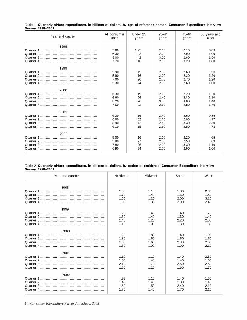
64 Consumer Expenditure Survey Anthology, 2005
Table 1. Quarterly airfare expenditures, in billions of dollars, by age of reference person, Consumer Expenditure InterviewSurvey, 1998–2002
1998Quarter 1 ................................................................ 5.60 0.25 2.30 2.10 0.89Quarter 2 ................................................................ 6.30 .22 2.20 2.90 1.00Quarter 3 ................................................................ 8.00 .42 3.20 2.80 1.50Quarter 4 ................................................................ 7.70 .16 2.50 3.20 1.80
1999Quarter 1 ................................................................ 5.90 .19 2.10 2.60 .90Quarter 2 ................................................................ 5.90 .16 2.00 2.20 1.20Quarter 3 ................................................................ 7.00 .26 2.70 2.70 1.20Quarter 4 ................................................................ 5.30 .24 2.00 2.60 1.00
2000Quarter 1 ................................................................ 6.30 .19 2.60 2.20 1.20Quarter 2 ................................................................ 6.60 .26 2.40 2.80 1.10Quarter 3 ................................................................ 8.20 .26 3.40 3.00 1.40Quarter 4 ................................................................ 7.60 .22 2.80 2.80 1.70
2001Quarter 1 ................................................................ 6.20 .16 2.40 2.60 0.89Quarter 2 ................................................................ 6.00 .32 2.60 2.00 .97Quarter 3 ................................................................ 8.90 .42 2.80 3.30 2.30Quarter 4 ................................................................ 6.10 .15 2.60 2.50 .78
2002Quarter 1 ................................................................ 5.00 .16 2.00 2.20 .65Quarter 2 ................................................................ 5.80 .27 2.30 2.50 .69Quarter 3 ................................................................ 7.80 .26 2.90 3.30 1.10Quarter 4 ................................................................ 6.90 .24 2.70 2.90 1.00
All consumerunits
Under 25yearsYear and quarter
25–44years
45–64years
65 years andolder
Table 2. Quarterly airfare expenditures, in billions of dollars, by region of residence, Consumer Expenditure InterviewSurvey, 1998–2002
1998Quarter 1 ........................................................................ 1.00 1.10 1.30 2.00Quarter 2 ........................................................................ 1.70 1.40 1.30 1.80Quarter 3 ........................................................................ 1.60 1.20 2.00 3.10Quarter 4 ........................................................................ 1.90 1.30 2.00 2.40
1999Quarter 1 ........................................................................ 1.20 1.40 1.40 1.70Quarter 2 ........................................................................ 1.60 1.40 1.30 1.40Quarter 3 ........................................................................ 1.40 1.20 2.20 2.00Quarter 4 ........................................................................ 1.10 1.00 1.30 1.80
2000Quarter 1 ........................................................................ 1.20 1.80 1.40 1.90Quarter 2 ........................................................................ 1.80 1.60 1.50 1.60Quarter 3 ........................................................................ 1.60 1.60 2.30 2.60Quarter 4 ........................................................................ 1.60 1.90 1.90 2.10
2001Quarter 1 ........................................................................ 1.10 1.10 1.40 2.30Quarter 2 ........................................................................ 1.50 1.40 1.40 1.60Quarter 3 ........................................................................ 2.10 1.70 2.50 2.50Quarter 4 ........................................................................ 1.50 1.20 1.60 1.70
2002Quarter 1 ........................................................................ .99 1.10 1.40 1.50Quarter 2 ........................................................................ 1.40 1.40 1.30 1.40Quarter 3 ........................................................................ 1.50 1.50 2.40 2.10Quarter 4 ........................................................................ 1.70 1.40 1.70 2.10
Year and quarter Northeast Midwest South West
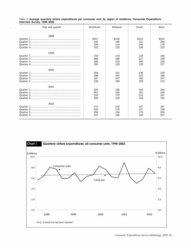
Consumer Expenditure Survey Anthology, 2005 65
Chart 1. Quarterly airfare expenditures, all consumer units, 1998—2002
1998 1999 2000 2001 2002
$ billions $ billions
0.0
2.0
4.0
6.0
8.0
10.0
0.0
2.0
4.0
6.0
8.0
10.0
NOTE: A trend line has been inserted.
Consumer units
Trend line
Table 3. Average quarterly airfare expenditures per consumer unit, by region of residence, Consumer ExpenditureInterview Survey, 1998–2002
1998Quarter 1 ........................................................................ $157 $139 $115 $214Quarter 2 ........................................................................ 242 166 121 200Quarter 3 ........................................................................ 200 114 146 278Quarter 4 ........................................................................ 232 115 158 223
1999Quarter 1 ........................................................................ 218 178 129 180Quarter 2 ........................................................................ 268 168 127 150Quarter 3 ........................................................................ 186 119 165 192Quarter 4 ........................................................................ 200 128 135 227
2000Quarter 1 ........................................................................ 204 221 138 218Quarter 2 ........................................................................ 298 181 163 190Quarter 3 ........................................................................ 197 157 183 247Quarter 4 ........................................................................ 238 188 158 213
2001Quarter 1 ........................................................................ 226 139 144 264Quarter 2 ........................................................................ 261 160 152 190Quarter 3 ........................................................................ 310 173 214 247Quarter 4 ........................................................................ 200 129 148 162
2002Quarter 1 ........................................................................ 174 145 137 167Quarter 2 ........................................................................ 249 178 127 169Quarter 3 ........................................................................ 206 154 179 202Quarter 4 ........................................................................ 247 146 149 207
Year and quarter Northeast Midwest South West
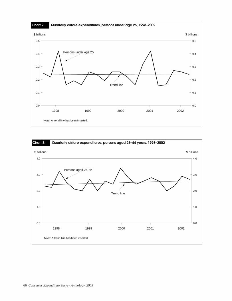
66 Consumer Expenditure Survey Anthology, 2005
Chart 2. Quarterly airfare expenditures, persons under age 25, 1998—2002
1998 1999 2000 2001 2002
$ billions $ billions
0.0
0.1
0.2
0.3
0.4
0.5
0.0
0.1
0.2
0.3
0.4
0.5
NOTE: A trend line has been inserted.
Persons under age 25
Trend line
Chart 3. Quarterly airfare expenditures, persons aged 25—44 years, 1998—2002
1998 1999 2000 2001 2002
$ billions $ billions
0.0
1.0
2.0
3.0
4.0
0.0
1.0
2.0
3.0
4.0
NOTE: A trend line has been inserted.
Persons aged 25–44
Trend line
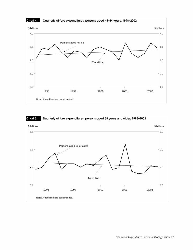
Consumer Expenditure Survey Anthology, 2005 67
Chart 4. Quarterly airfare expenditures, persons aged 45—64 years, 1998—2002
1998 1999 2000 2001 2002
$ billions $ billions
0.0
1.0
2.0
3.0
4.0
0.0
1.0
2.0
3.0
4.0
NOTE: A trend line has been inserted.
Persons aged 45–64
Trend line
Chart 5. Quarterly airfare expenditures, persons aged 65 years and older, 1998—2002
1998 1999 2000 2001 2002
$ billions $ billions
0.0
1.0
2.0
3.0
0.0
1.0
2.0
3.0
NOTE: A trend line has been inserted.
Persons aged 65 or older
Trend line
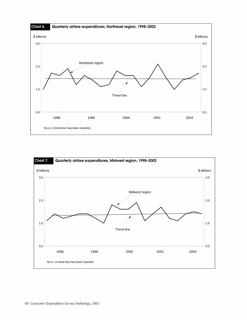
68 Consumer Expenditure Survey Anthology, 2005
Chart 6. Quarterly airfare expenditures, Northeast region, 1998—2002
1998 1999 2000 2001 2002
$ billions $ billions
0.0
1.0
2.0
3.0
0.0
1.0
2.0
3.0
NOTE: A trend line has been inserted.
Northeast region
Trend line
Chart 7. Quarterly airfare expenditures, Midwest region, 1998—2002
1998 1999 2000 2001 2002
$ billions $ billions
0.0
1.0
2.0
3.0
0.0
1.0
2.0
3.0
NOTE: A trend line has been inserted.
Midwest region
Trend line
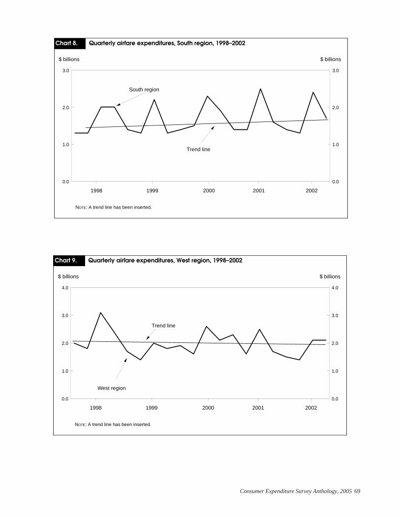
Consumer Expenditure Survey Anthology, 2005 69
Chart 8. Quarterly airfare expenditures, South region, 1998—2002
1998 1999 2000 2001 2002
$ billions $ billions
0.0
1.0
2.0
3.0
0.0
1.0
2.0
3.0
NOTE: A trend line has been inserted.
South region
Trend line
Chart 9. Quarterly airfare expenditures, West region, 1998—2002
1998 1999 2000 2001 2002
$ billions $ billions
0.0
1.0
2.0
3.0
4.0
0.0
1.0
2.0
3.0
4.0
NOTE: A trend line has been inserted.
West region
Trend line
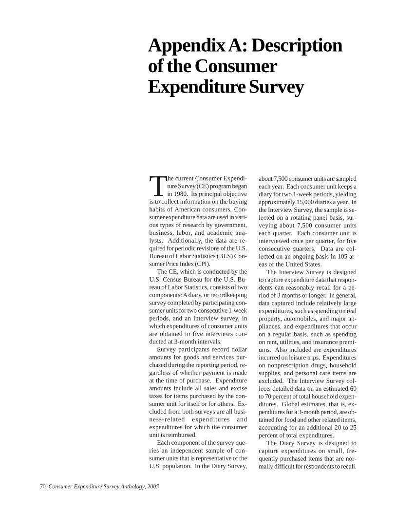
70 Consumer Expenditure Survey Anthology, 2005
Appendix A: Descriptionof the ConsumerExpenditure Survey
The current Consumer Expendi-ture Survey (CE) program beganin 1980. Its principal objective
is to collect information on the buyinghabits of American consumers. Con-sumer expenditure data are used in vari-ous types of research by government,business, labor, and academic ana-lysts. Additionally, the data are re-quired for periodic revisions of the U.S.Bureau of Labor Statistics (BLS) Con-sumer Price Index (CPI).
The CE, which is conducted by theU.S. Census Bureau for the U.S. Bu-reau of Labor Statistics, consists of twocomponents: A diary, or recordkeepingsurvey completed by participating con-sumer units for two consecutive 1-weekperiods, and an interview survey, inwhich expenditures of consumer unitsare obtained in five interviews con-ducted at 3-month intervals.
Survey participants record dollaramounts for goods and services pur-chased during the reporting period, re-gardless of whether payment is madeat the time of purchase. Expenditureamounts include all sales and excisetaxes for items purchased by the con-sumer unit for itself or for others. Ex-cluded from both surveys are all busi-ness-related expenditures andexpenditures for which the consumerunit is reimbursed.
Each component of the survey que-ries an independent sample of con-sumer units that is representative of theU.S. population. In the Diary Survey,
about 7,500 consumer units are sampledeach year. Each consumer unit keeps adiary for two 1-week periods, yieldingapproximately 15,000 diaries a year. Inthe Interview Survey, the sample is se-lected on a rotating panel basis, sur-veying about 7,500 consumer unitseach quarter. Each consumer unit isinterviewed once per quarter, for fiveconsecutive quarters. Data are col-lected on an ongoing basis in 105 ar-eas of the United States.
The Interview Survey is designedto capture expenditure data that respon-dents can reasonably recall for a pe-riod of 3 months or longer. In general,data captured include relatively largeexpenditures, such as spending on realproperty, automobiles, and major ap-pliances, and expenditures that occuron a regular basis, such as spendingon rent, utilities, and insurance premi-ums. Also included are expendituresincurred on leisure trips. Expenditureson nonprescription drugs, householdsupplies, and personal care items areexcluded. The Interview Survey col-lects detailed data on an estimated 60to 70 percent of total household expen-ditures. Global estimates, that is, ex-penditures for a 3-month period, are ob-tained for food and other related items,accounting for an additional 20 to 25percent of total expenditures.
The Diary Survey is designed tocapture expenditures on small, fre-quently purchased items that are nor-mally difficult for respondents to recall.
Consumer Expenditure Survey Anthology, 2005 71
Detailed records of expenses are keptfor food and beverages—both at homeand in eating places—tobacco, house-keeping supplies, nonprescriptiondrugs, and personal care products andservices. Expenditures incurred awayfrom home overnight or longer are ex-cluded from the Diary Survey. Al-though the diary was designed to col-lect information on expenditures thatcould not be recalled easily over a pe-riod of time, respondents are asked toreport all expenses (except overnighttravel expenses) that the consumer unitincurs during the survey week.
Integrated data from the BLS Diaryand Interview Surveys provide a com-plete accounting of consumer expen-ditures and income, which neither sur-vey component alone is designed todo. Data on some expenditure itemsare collected in only one of the compo-nents. For example, the Diary Surveydoes not collect data on expendituresfor overnight travel or information onthird-party reimbursements of con-sumer expenditures, as the InterviewSurvey does. Examples of expendituresfor which reimbursements are excludedare medical care; automobile repair; andconstruction, repairs, alterations, andmaintenance of property.
For items unique to one or the othersurvey, the choice of which survey touse as the source of data is obvious.However, there is considerable over-lap in coverage between the surveys.Because of this overlap, integratingdata presents the problem of determin-ing the appropriate survey componentfrom which to select expenditure items.When data are available from both sur-vey sources, the more reliable of thetwo (as determined by statistical meth-ods) is selected. As a result, some itemsare selected from the Interview surveyand others from the Diary Survey.
Population coverage and the defi-nition of components of the CE differfrom those of the CPI. Consumer ex-penditure data cover the total popu-lation, whereas the CPI covers only theurban population. In addition, homeownership is treated differently in thesetwo surveys. Actual expenditures ofhomeowners are reported in the CE,
whereas the CPI uses a rental equiva-lence approach that attempts to mea-sure the change in the cost of obtain-ing, in the rental marketplace, servicesequivalent to those provided by owner-occupied homes.
Interpreting the dataExpenditures are averages for con-sumer units with specified characteris-tics, regardless of whether a particularunit incurred an expense for a specificitem during the recordkeeping period.The average expenditure for an itemmay be considerably lower than theexpenditure by those consumer unitsthat actually purchased the item. Theless frequently an item is purchased,the greater the difference between theaverage for all consumer units and theaverage for those purchasing the item.Also, an individual consumer unit mayspend more or less than the average,depending on its particular character-istics. Factors such as income, ages offamily members, geographic location,taste, and personal preference influ-ence expenditures. Furthermore, evenwithin groups with similar characteris-tics, the distribution of expendituresvaries substantially. These pointsshould be considered when relatingreported averages to individual circum-stances.
In addition, sample surveys are sub-ject to two types of errors: samplingand nonsampling. Sampling errors oc-cur because the data are collected froma representative sample rather than theentire population. Nonsampling errorsresult from the inability or unwilling-ness of respondents to provide correctinformation, differences in interviewers’abilities, mistakes in recording or cod-ing, or other processing errors.
Glossary
Consumer unit. Members of a house-hold related by blood, marriage, adop-tion, or some other legal arrangement;a single person living alone or sharinga household with others, but who isfinancially independent; or two or morepersons living together who share re-sponsibility for at least two out of three
major types of expenses: Food, hous-ing, and other expenses. Students liv-ing in university-sponsored housingare also included in the sample as sepa-rate consumer units.
Reference person. The first membermentioned by the respondent whenasked to “Start with the name of theperson or one of the persons who ownsor rents the home.” It is with respect tothis person that the relationship ofother members of the consumer unit isdetermined.
Total expenditures. The transactioncosts, including excise and sales taxes,of goods and services acquired duringthe interview period. Estimates includeexpenditures for gifts and contribu-tions and payments for pensions andpersonal insurance.
Income. The combined income earnedby all consumer unit members 14 yearsor older during the 12 months preced-ing the interview. The components ofincome are wages and salaries; self-employment income; Social Securityand private and government retirementincome; interest, dividends, and rentaland other property income; unemploy-ment and workers’ compensation andveterans’ benefits; public assistance,Supplemental Security Income (SSI),and Food Stamps; rent or meals or bothas pay; and regular contributions forsupport, such as alimony and childsupport.
Complete income reporters. In gen-eral, a consumer unit that provides val-ues for at least one of the major sourcesof its income, such as wages and sala-ries, self-employment income, and So-cial Security income. Even completeincome reporters may not provide a fullaccounting of all income from allsources.
Quintiles of income before taxes.Complete income reporters are rankedin ascending order of income value anddivided into five equal groups. Incom-plete income reporters are not rankedand are shown separately in thequintiles of income tables.