Planning ahead: consumer expenditure patterns in retirement · Planning ahead: consumer expenditure patterns in retirement ... Rose Rubin and Michael Nieswiadomy compare ... Planning

38 Monthly Labor Review July 2002

Expenditures in RetirementExpenditures in Retirement

Planning ahead: consumerexpenditure patterns in retirement

The ‘graying’ of the population createsa need to examine the rolethat retirement plays on expenditure decisionsof various demographic groups of retirees

Geoffrey D. PaulinandAbby L. Duly

Geoffrey D. Paulinis a senior economist,and Abby L. Dulyis an economist,Division of ConsumerExpenditure Surveys,Bureau of LaborStatistics.Email:[email protected][email protected]

The fastest growing segment of the U. S.population is composed of those aged 65and older. The Bureau of the Census re-

ported that in 1994, 1 in 8 Americans was in thisage group, but projects that the ratio may be ashigh as 1 in 5 by 2050. Furthermore, with in-creases in life expectancy, today’s adults will livean average of 17 additional years after reachingage 65.1

As this demographic pattern shifts, an in-creasing demand for research and data on theolder population—specifically, on retired per-sons and their roles on consumers—is con-stantly in evidence: “baby boomers,”“privatization of Social Security,” “Medicare,”and tips on financial planning are common top-ics of the daily print and video media. The sheergrowth in numbers suggests that the spendingpatterns of this older population will also playan increasingly important role in the futureeconomy, an assumption supported by recenttrends in expenditure levels. A study of real (thatis, inflation-adjusted) expenditures from 1984 to1997 finds that “spending by older consumershas risen from 12.6 percent to 14.6 percent of allconsumer spending.”2

In addition to the concerns these issues mayraise for policymakers, especially those involvedwith providing adequate care and protection forolder consumers, the decision to retire has majorimplications for individuals and families. Under-standing differences in spending patterns for

preretired and retired consumers can help work-ers plan for the future.

Taken together, these items suggest that astudy of expenditure patterns of retirees is war-ranted. Differences in expenditure patterns forpreretirees and retirees are expected for many rea-sons. For example, income presumably will de-cline upon retirement. Given the relationship ofincome to expenditures, it is important to see howincome differs—in level as well as in sources ofreceipt. Also, other demographic characteristicspresumably play an important role in expendituredecisions, both before and after retirement.Therefore, examining the role these characteris-tics play is also important. In looking at spend-ing patterns for families who are near retirementand comparing them with the patterns of thoseindividuals who have actually exited from theworkforce, this article provides valuable informa-tion about the impact of retirement on consumerspending.

Several issues are addressed here. First, back-ground describing related research is presented.Second, data from the U.S. Consumer Expendi-ture Survey, which provide the basis for theanalysis, are described. Third, demographic char-acteristics of “preretired” and “retired” consum-ers in this sample are presented and compared.Fourth, income and expenditure patterns are de-scribed for these groups. Finally, regressionanalysis is used to explore differences in expen-diture patterns given that demographics and in-

Monthly Labor Review July 2002 39

come levels are different for preretired and retired consumers.(Logit and ordinary least squares results for the two groupsare presented in a detailed appendix.)

Related research

Many previous studies related to the population aged 65 andolder can be divided into two groups: those that focus onage, and those that focus on retirement. Both groups areimportant, and both have contributed to the analyses pre-sented here.

Expenditure patterns by age. Rose Rubin and Kenneth Koelinexamine how elderly households spend on necessities, com-pared with nonelderly households.3 Using data from the 1980–81 and 1989–90 Consumer Expenditure Survey, they examineexpenditures for housing, food at home, and healthcare, aswell as income, demographics, and receipt of cash assistance(AFDC or SSI). The methodology used to examine the relation-ship between their variables of interest is based on the lifecycle theory of consumption, with total expenditures actingas a proxy for permanent income. Rubin and Koelin’s resultsindicate that, in general, older consumers spend a higher pro-portion of their budget on housing and healthcare than do thenonelderly, and that the receipt of financial assistance doesplay a role in the spending decisions of both age groups.

In a study of age groups within the older population,Mohammed Abdel-Ghany and Deanna Sharpe use Tobit analy-sis to determine whether tastes and preferences differ for thoseaged 65 to 74 and those aged 75 and older.4 Using indepen-dent variables such as total expenditures (once again as asurrogate for permanent income), region of residence, educa-tion of reference person,5 household size, race, and familytype, the authors find differences between the “young-old”and “old-old” (as they term the groups) across all major cat-egories of expense. Furthermore, the effect of the socioeco-nomic variables on spending patterns differed between thetwo age groups, and among spending categories.

Studies based on retirement status. Because this study com-pares retired households with those that have members near-ing retirement, previous studies based on work status are dis-cussed in more detail. Among the studies reviewed here, anarticle by Nancy E. Schwenk is unique in its focus on thelevels and sources of income of retirees, using multiple gov-ernment surveys as sources.6 Schwenk provides some dis-cussion of expenditures, specifically the fact that the alloca-tion of total spending for retirement, pensions, and SocialSecurity is significantly less for households in which the ref-erence person has “reached retirement age (65 years or older)”than for those in which the reference person is aged 45 to 54.In terms of demographics, she notes that the majority of con-

sumers aged 65 years and older own their home, and that “ofthose who are homeowners, most owned their home free andclear (81 percent).” Finally, Schwenk finds that in 1991, in-come from dividends, interest, and rent provided about 20percent of retirees’ total income.7

An earlier article by Frankie N. Schwenk uses data from the1987 Consumer Expenditure Survey to examine whether thereare differences between those who opt for “early retirement”and those who continue to work beyond the age of 65.8 Inthis study, F. Schwenk specifically compares the two groupsin terms of family characteristics, asset levels, income, andexpenditures. Using Probit analysis, the author finds thatage, spouse’s employment status, education, housing tenure,household size, marital status, and gender are significant fac-tors in predicting the likelihood of being retired. Other com-parisons show that “average dividend and interest [income]amounts were higher for retired than for working families,”and that “health was the only category of expenditures forwhich households with a retired reference person spent morethan those with an employed person.”9

In a May 1990 article, Thomas Moehrle uses the Con-sumer Expenditure Survey to compare the average annualexpenditures of elderly working and nonworking consumerunits10 across low, medium, and high income groups. 11

Moehrle finds that (1) “Nonworking elderly householdsspend more on food prepared at home than do working eld-erly households, regardless of income level,” and (2) “Re-gardless of income level, nonworking elderly householdsspend more on health care than do working elderly house-holds.”12 Note that Moehrle analyzes one age group, thosewith a reference person aged 62 to 74, and that the workingstatus of the consumer unit is based solely on that of thereference person, regardless of whether any other membersare working or not. Also, he does not specifically limit thenonworking households to those whose reference person isretired (for example, “nonworking” can mean the referenceperson is disabled, taking care of the home or family, or goingto school). However, he finds that “79 percent [of the non-working consumer units studied] had reference persons whoclassified themselves as retired.”13

Rose Rubin and Michael Nieswiadomy compare demo-graphic characteristics, income, and expenditures of retireesand nonretirees aged 50 or older from the 1986 and 1987 Con-sumer Expenditure Survey.14 Their sample consists of com-plete income reporters only, with the retirement status basedon that of the respondent.15 Rubin and Nieswiadomy alsodivide their sample into three household types: single men,single women, and husband-wife couple households. UsingTobit regression analysis, they find “that the retired have ahigher marginal propensity to spend (than the nonretired) forfood, alcohol, housefurnishings, apparel, transportation, gasand motor oil, other vehicles, public transportation, health


Expenditures in Retirement

care, entertainment, and cash gifts.”16 Also noteworthy istheir conclusion that for both the retired and nonretiredhouseholds, healthcare expenditures increase with educa-tional attainment.

About the sample

This article uses data from the 1998 and 1999 Consumer Ex-penditure Interview Surveys. The Interview Survey is a rotat-ing panel survey designed to collect information on majoritems of expense, household characteristics, and income. Thequestionnaire is administered to sample consumer units onceper quarter for five consecutive quarters. The main goal ofthe initial household interview is to collect inventory informa-tion to be used for bounding purposes, that is, to ensure thatexpenditures reported in subsequent interviews took placeduring the appropriate reference period (in most cases, thiswill be the 3-month period prior to the interview date). Whileit is primarily designed to collect large (vehicles or appliances,for example) and recurring (such as, rent or utilities) expendi-tures that can be easily recalled on a quarterly basis, the Inter-view Survey captures up to 95 percent of all expenditures.17

In order to examine the effect of retirement on consumerspending patterns, the sample is divided into two groups: apreretired group and a retired group. Ultimately, it would bemost useful to have data for the same family over some pe-riod of time to observe their expenditures both before andafter retirement and compare them directly. Unfortunately, asdiscussed, the survey is not designed to follow families forextended time periods. Even using multiple years of data, itwould be difficult to find families who are “working” in atleast one quarter and then “retired” for the remainingquarter(s) of their participation. The results described here,then, must be interpreted cautiously, bearing this in mind.Nevertheless, the sample has been selected in such a way asto make these comparisons as appropriately as possible, giventhe data constraints.

To this end, a preretired consumer unit is defined as onewhose reference person is aged 55 to 64, and is earning atleast one type of labor income (that is, wage and salary in-come or self-employment income). This age group is chosenbecause, for many, it is the last stage of their working lives.Although some may choose to retire prior to reaching age 65,this study excludes any consumer unit from the “preretired”category in which there is a retired person (including aspouse). In contrast, a “retired” consumer unit is defined asone whose reference person is aged 65 to 74 and who is re-tired; that is, when asked about the occupation for which theyreceived the most income, they report that they are not work-ing due to retirement. Additionally, there are no earners in the“retired” households. Excluded from both groups (preretiredand retired) are families in which the spouse (if present) is not

working either due to illness or disability, or due to unemploy-ment. This omission is made because a consumer unit with adisabled member may have some vastly different spendingpatterns than an otherwise similar household, such as medi-cal expenses. Furthermore, in the case of illness or disability,the decision not to work is not necessarily a voluntary one,but rather is the result of circumstances that make work im-possible.18 Similarly, an unemployed person presumably wouldlike to work, and may eventually do so; therefore, these fami-lies may not display the same consumer expenditure patternsas those in which the spouse is not working for voluntaryreasons (such as retirement or taking care of the home orfamily).19 The age groups are chosen to compare those on theverge of retirement with those consumer units who have re-cently retired, allowing these analyses to focus on the effectof retirement as a single discrete event. Furthermore, previ-ous research has shown that there are significant differencesbetween those aged 65 to 74 and those aged 75 and older interms of household characteristics, income, and expendi-tures.20 Therefore, the consumer units whose reference per-son is aged 75 or older are removed from the retired sample inorder to eliminate this age effect.21

To facilitate the analysis, the sample for this study is lim-ited in scope. First, the sample is limited to three types ofhouseholds: single men, single women, and husband-and-wife couples. These groups are selected in order to reducethe effect of family size on expenditure patterns. Additionally,the effects of other family member characteristics on expendi-tures are eliminated. For example, preretired families with chil-dren may be spending differently than those without chil-dren, because they may be expecting to send the children tocollege soon. Retired families with children may be supportedby these children.22 In either case, expenditures would bedifferent from those who have children of different age, futureplans, and so forth.23 Even so, families with children are pre-sumably the exception, rather than the rule for these families,especially those who are retired.

The separation of single men and single women is done inorder to examine the effect of gender-related differences onspending patterns. For example, in terms of income, the life-time earnings of men and women are expected to be quitedifferent, especially given the generation being examined. Also,marital status is affected by differences in life expectancy (thatis, there are more widowed single women than there are malewidowers, as shown in table 1). These factors presumablywill have an influence on spending patterns.

The type of household is determined by two pieces ofinformation: the number of family members and the maritalstatus of the reference person. For husband-and-wife couples,the values for these variables are obvious: that is, there aretwo persons in the consumer unit (one of which, by defini-tion, must be the reference person) and the marital status of


Demographics of preretirees and retirees, by composition of consumer unit, Consumer Expenditure InterviewSurvey, 1998–99

Characteristic

Table 1.

Number of consumer units ................... 260 222 – 547 725 – 1,325 1,220 –

Age of reference person ...................... 59 70 41.976 59 70 73.192 59 70 99.809

Average number of:Rooms:

Renter ......................................... 4.0 3.0 4.590 4.4 3.9 3.396 4.8 4.6 .795Homeowner ................................... 5.8 5.9 .650 5.7 5.8 .823 6.9 6.4 7.494

Bathrooms (including halfbaths):Renter ......................................... 1.1 1.1 .102 1.3 1.2 1.458 1.4 1.6 2.307Homeowner ................................... 1.7 1.7 .113 1.8 1.7 1.261 2.2 2.0 5.020

Vehicles ............................................ 1.9 1.9 .272 1.2 1.2 1.961 2.7 2.3 6.384Automobiles .................................... 1.3 1.2 2.397 1.1 1.1 2.053 1.6 1.4 6.501Other vehicles ................................. .6 .7 .859 .1 .1 1.159 1.1 .9 3.419

PercentHousing tenure:

Homeowner:With mortgage ........................... 31.9 7.7 – 40.0 11.5 – 51.6 16.6 –With no mortgage ....................... 29.6 64.0 – 35.8 68.3 – 41.0 78.2 –

Renter ......................................... 38.5 28.4 – 24.1 20.3 – 7.4 5.3 –

Occupation of reference person:Working for wage or salary ................ 91.1 0 – 94.1 0 – 85.6 0 –Self-employed .................................. 8.9 0 – 5.9 0 – 14.4 0 –Retired ........................................... 0 100.0 – 0 100.0 – 0 100.0 –

Marital status of reference person:Married ........................................... 3.5 6.3 – 4.6 4.0 – 100.0 100.0 –Widowed ......................................... 11.9 43.2 – 27.4 71.7 – 0 0 –Divorced ......................................... 56.2 32.9 – 53.0 17.2 – 0 0 –Separated ....................................... 7.7 3.6 – 3.1 .7 – 0 0 –Single (never married) ....................... 20.8 14.0 – 11.9 6.3 – 0 0 –

Race/ethnicity of reference person:Black .............................................. 12.7 13.5 – 13.2 7.6 – 5.3 4.3 –Hispanic ......................................... 4.6 3.2 – 2.2 1.5 – 3.0 1.8 –White and other ............................... 82.7 83.3 – 84.6 90.9 – 91.7 93.9 –

Education of reference person:Did not graduate high school ............. 10.8 30.6 – 11.3 20.0 – 9.2 18.8 –High school graduate ........................ 30.8 27.5 – 29.6 38.6 – 33.0 33.0 –Some college (including A.A. degree) .................. 23.5 16.2 – 33.6 24.7 – 26.9 22.3 –College graduate (B.A. degree, and so forth) ................................ 22.3 15.3 – 14.6 10.9 – 16.2 17.9 –Graduate/professional degree ............ 12.7 10.4 – 10.8 5.9 – 14.7 8.1 –

Degree urbanization:Rural .............................................. 6.9 9.5 – 10.8 11.6 – 13.2 13.9 –Urban ............................................. 93.1 90.5 – 89.2 88.4 – 86.8 86.1 –

Region of residence:Northeast ........................................ 18.8 23.0 – 13.2 20.3 – 18.2 20.6 –Midwest .......................................... 17.3 28.8 – 24.5 23.2 – 29.9 25.3 –South ............................................. 39.2 22.1 – 39.3 36.3 – 33.4 33.5 –West .............................................. 24.6 26.1 – 23.0 20.3 – 18.6 20.6 –

Income distribution:1st quintile ...................................... 10.2 36.4 – 17.1 50.2 – 4.1 9.2 –2nd quintile ..................................... 20.4 35.8 – 33.1 35.0 – 6.4 46.0 –3rd quintile ...................................... 27.3 13.9 – 26.3 12.1 – 16.6 28.6 –4th quintile ...................................... 26.9 8.1 – 16.7 2.2 – 26.9 12.4 –5th quintile ...................................... 15.3 5.8 – 6.8 .5 – 46.2 3.8 –

1 Absolute values are displayed.

Single men Single women Married couples

Preretired Preretired PreretiredRetired Retired Retiredt-value 1 t-value 1 t-value 1



the reference person is married. For single-member consumerunits, however, there are a variety of possible values for themarital status variable. A single man or woman may be wid-owed, divorced, separated, never married, or in a small num-ber of cases, married. Even though a “married single person”seems oxymoronic, some plausible explanations exist. Con-sidering that the household type is determined at the time ofthe interview, a married person whose spouse is living else-where (perhaps on a long-term work assignment, such as amilitary tour of duty) may be counted as a single person con-sumer unit. It could also be that some of these “marriedsingles” are actually separated, though perhaps not legallyso. In that case, the respondent may identify himself or her-self as married, rather than separated. Either way, the spend-ing patterns of a married person living alone for an extendedperiod are assumed to mirror the spending patterns of a “true”single person more closely than those of a married couple.

The sample also includes only those consumer units thatreport ownership of at least one automobile, so that expendi-tures will be more comparable. The most obvious effect ofautomobile ownership is on transportation expenditures. Pre-sumably, some retirees choose to sell or give away their auto-mobiles due to a lack of need for personal transportation (forexample, they are no longer going out to work every day).Maintaining an automobile can add many dollars of expendi-ture to the household budget. Not only are there costs forgasoline, motor oil, and the occasional repair, but automobileinsurance may be expensive, and may increase as the drivergrows older. Age-related health reasons may also play a partin this decision. Whatever the reason, lack of automobileownership presumably limits mobility, and thus may affectother expenditures, such as those for food away from home,entertainment, and vacation and travel.

The above qualifications result in the following samplesizes: 260 preretired single men and 222 retired single men;547 preretired single women and 725 retired single women;and 1,325 preretired couples and 1,220 retired couples. Notethat these data are not weighted to reflect the population.

First, this article compares demographics, income, and quar-terly expenditures of preretired and retired consumer units,within each household type examined (that is, single personor married couple). Some of the results of these comparisonsmay be expected based on the parameters set for each group.For example, the lower income levels reported for retirees arenot surprising given that no one is earning labor income inthose households. Thus, an important question is how retire-ment itself affects expenditure patterns: that is, whether tastesand preferences change in retirement, even if incomes are heldconstant. To this end, regression analysis is performed (us-ing ordinary least squares and a modified Cragg method wherenecessary) to examine differences in marginal propensity to

consume and income elasticity. These analyses help to es-tablish whether or not differences in expenditure patterns arerelated to retirement, per se, or to an income effect associatedwith retirement.

Demographics

As previously noted, some of the household characteristicsare determined by the sample selection criteria. For example,the average age of the reference person is constrained to bewithin the allowed ranges for the preretired group (55 to 64)and retired group (65 to 74). Across the three householdtypes studied, the average age for preretired reference per-sons is 59 years, and that for retired reference persons is 70years. (See table 1.) Additionally, because automobile owner-ship is a condition of the sample selection process, the aver-age number of vehicles is greater than one in each case.

However, some findings are not so predictable. For ex-ample, contrary to the popular notion that “everyone” movesto Florida (or at least the “Sunbelt”) upon retirement, singlepreretirees are more likely to be located in the South thansingle retirees. This difference is most pronounced for singlemen: 39 percent of preretirees live in the South, compared with22 percent of retirees. For single women, the difference is lesspronounced: 39 percent of preretirees live in the South, com-pared with 36 percent of retirees. However, for married couples,almost no difference exists; about one-third of married couplesstudied live in the South both before and after retirement.

Single men. Single retired men are more likely to behomeowners (72 percent) than are single preretired men (62percent). The difference is even more pronounced if the ho-meowner holds no mortgage against his property: 64 percentof single male retirees own their homes outright, comparedwith only 30 percent of the preretired. Regardless of workstatus, more than 90 percent of single men live in urban areas.Additionally, despite the large plurality of preretired singlemen in the South (39 percent), after retirement, single menhave the most even distribution of the study sample. Ironi-cally, the South has the lowest percentage of retired men—22percent. It is the Midwest that claims the highest percentageof single retired men (29 percent).

There is little difference between single male retirees andsingle male preretirees in terms of race or ethnicity. Morethan 80 percent of both groups have reference persons whoare white (or other race, including Asian, Pacific Islander, andothers), and the least represented race for both groups isHispanic (3 percent of retired and 5 percent of preretired singlemen).

For single retired men, the distributions among levels ofeducation and among income quintiles follow the same nega-


tive slope. For example, the largest percentage of single re-tired men (31 percent) has attained the least education, that is,they did not graduate from high school. Similarly, the largestproportion of single male retirees are also in the lowest in-come quintile (36 percent). Furthermore, the highest categoryof educational attainment (graduate or professional degree)accounts for the smallest proportion of single retired men (10percent), and the highest income quintile contains the small-est proportion of single retired men (6 percent). Given theexpected correlation between income and education, this pat-tern is not surprising. The correlation also appears to hold forsingle preretired men, although the ordering of categories isreversed: single preretired men are more likely to have at leasta high school degree than are single retired men, and they arealso more likely to be in one of the top three quintiles than aresingle retired men. This may reflect a generational effect, aseducational opportunities have become more available andmore socially and economically valuable for each successivegeneration.

Single women. The housing tenure and degree of urbaniza-tion for single women follow the same patterns as those de-scribed for single men, that is, retirees are more likely to behomeowners without a mortgage than are preretirees, and re-gardless of work status the majority of the sample resides inurban rather than rural areas. However, unlike single men, ahigher percentage of single women, both retired and working,live in the South (36 percent of single retired women and 39percent of single preretired women) compared with other re-gions. It is also interesting to note that the largest differencein the proportion of retired and preretired single female resi-dents is in the Northeast. Only 13 percent of (or about one ineight) single female preretirees live in this region, comparedwith 20 percent of (or one in five) single female retirees.

In terms of race, again, white and other is the predominantgroup for both single female retirees (91 percent) and singlefemale preretirees (85 percent). There is, however, a notabledifference in the proportion of single female retirees who areblack (8 percent) and single female preretirees who are black(13 percent). Roughly 2 percent of both groups of singlewomen are Hispanic.

Unlike single retired men, the largest percentage of singleretired women have completed high school (39 percent), com-pared with other levels of education, but only 6 percent haveobtained a graduate or professional degree. Again, those inthe preretired group are more likely than retirees to have atleast attended college. While the income distribution for singleretired women is similar to that of single retired men, the dis-parity between the lowest and highest quintiles is much greaterfor single women. In fact, half of all single retired women fallinto the lowest quintile, and less than 1 percent fall into the

highest quintile. More single preretired women are in thesecond income quintile (33 percent) than are in any otherquintile, and a much higher percentage of preretirees (7 per-cent) than retirees fall into the highest income quintile.

Husband-and-wife couples. Once again, homeownership ismore likely in the retired sample than in the preretired sampleof married couples. Furthermore, there is a lower percentageof renters in the married couple sample (5 percent of retireesand 7 percent of the preretired households) than in the singlessamples. Roughly one-third of husband-and-wife consumerunits live in the South, regardless of work status, and theMidwest is the only region in which the proportion of retiredmarried couples (25 percent) is smaller than that of preretiredmarried couples (30 percent).

There is little difference between retired married couplesand preretired married couples in the percentage of referencepersons who are white or other races, which is once again themost represented category in the sample.

Approximately one-third of the reference persons in bothretired and preretired husband/wife consumer units are highschool graduates. The largest differences between the twogroups are found at the lowest and highest levels of educa-tional attainment. While 19 percent of the retirees in thissample did not graduate from high school, the same is true foronly 9 percent of the preretired married couples. At the otherend of the scale, only 8 percent of reference persons in retiredcouples have earned a graduate or professional degree, com-pared with 15 percent of preretired couples.

The comparison of income distribution among retired andpreretired married couples is different from that of single menand that of single women. First, the highest percentage ofmarried retirees (46 percent) fall into the second quintile, notthe first quintile as is the case for single male and single fe-male retirees. In fact, only 9 percent of retired husband-and-wife households are in the lowest quintile. For the preretiredmarried couples, the income distribution is more concentrated,that is, only 4 percent of the sample are in the lowest quintileand 46 percent are in the highest income quintile.

Income

Before discussing the comparative results, it is important toprovide a more detailed definition of some of the incomesources examined in this study. For example, with income aswith demographics, there are some results that are determinedby the sample selection criteria. Specifically, no retired house-holds have labor income, including wages and salaries andself-employment income. For this reason, a new income cat-egory is created in order to make the total income for retireesand preretirees more comparable (income before taxes, which



is commonly used as a measure of total income, includes laborincome). The components of comparable income are thoseincome sources that are available to both retired and preretiredconsumer units: that is, comparable income includes interestand property income, unemployment insurance and workers’compensation, public assistance, and several other sources,but it excludes wages and salaries, self-employment income,or income from Social Security, and private and governmentretirement. It should be noted that more than 20 percent ofpreretirees in all three household types report some retire-ment income, which could be explained by early retirement.(See table 2.) Specifically, some persons may choose to retirefrom a career before age 65, but continue to earn some laborincome from another job; in this event, they are classified as

preretired in this study.24 Even so, retirement income is notincluded in the comparable measure, because it may be asupplemental source for the preretired, but it is the main (orperhaps sole) source of income for retirees, and thus it is notcomparable. Another important consideration regarding theincome analysis is that the figures presented are for averageannual income per consumer unit. To ensure more meaningfulcomparisons, only incomes from complete income reportersare shown.

Single men. Not surprisingly, single male retirees have sig-nificantly lower total incomes ($24,738) than do preretiredsingle men ($42,033). Approximately 77 percent of thepreretirees’ income is from wages and salaries ($32,196), while

Percent reporting and average annual income, preretirees and retirees, by composition of consumer unit,Consumer Expenditure Interview Survey, 1998–99 (complete income reporters only)

Table 2.

Percent reporting income source:Income before taxes ...................... 100.0 100.0 – 100.0 100.0 – 99.9 100.0 –

Wages and salaries ..................... 89.4 0 – 92.7 0 – 94.1 0 –Self-employment income ............... 14.8 0 – 6.1 0 – 19.9 0 –Social Security, private, and government retirement ......... 25.9 98.3 – 22.8 99.3 – 25.1 100.0 –Interest, dividends, rental income, and other property income .......... 37.5 35.3 – 31.2 27.4 – 32.3 36.9 –Unemployment, workers’ compensation, and veterans’ benefits ............... 5.6 3.5 – 3.8 .3 – 3.1 2.7 –Public assistance, supplemental security income, and food stamps ....................... .5 6.4 – 1.2 5.2 – .8 1.7 –Regular contributions for support (including child support and alimony) ............................. .5 0 – 2.8 2.1 – .2 .3 –Other income .............................. 3.2 1.7 – .2 .2 – 1.6 .8 –

Comparable income2 ....................... 42.6 41.6 – 36.4 34.3 – 36.0 39.8 –

Annual means:Income before taxes ...................... $42,033 $24,738 5.137 $30,443 $15,690 10.919 $74,816 $27,570 15.669

Wages and salaries ..................... 32,196 0 14.929 25,376 0 21.736 59,068 0 30.893Self-employment income3 ............. – 0 3.833 – 0 3.453 – 0 4.232Social Security, private, and government retirement ......... 3,482 17,815 10.722 2,177 13,758 24.149 4,533 25,038 33.288Interest, dividends, rental income, and other property income .......... 1,321 5,813 3.127 840 1,678 2.164 1,939 2,285 .878Unemployment, workers’ compensation, and veterans’ benefits ............... 392 172 .817 106 37 1.574 62 80 .607Public assistance, supplemental security income, and food stamps ....................... 2 106 2.027 14 60 2.243 44 94 0.888Regular contributions for support (including child support and alimony) ............................. 5 0 1.000 425 156 1.553 57 51 .093Other income .............................. 1,894 832 .929 0 1 .948 40 21 1.157

Comparable income2 ....................... 3,614 6,923 1.662 1,386 1,932 1.285 2,142 2,532 .961

CategorySingle men Single women Married couples


1 Absolute values are displayed.2 Income before taxes less wages and salaries; self-employment income; and Social Security, private and government retirement income.3 Mean incomes from this source are less than $1.


retirement income ($17,815) contributes 72 percent of the retir-ees’ income. However, when considering only comparableincome sources, the relationship between preretired and re-tired single men reverses. From those sources that are avail-able to both groups, retirees earn more ($6,923) than dopreretirees ($3,614). Yet, the percentage of single men report-ing these sources of comparable income is similar for the re-tired sample (42 percent) and the preretired sample (43 per-cent). Nevertheless, this “reversal of fortune” can be at leastpartially explained by the higher income earned by retired singlemen from dividends, interest, rental and other property—$5,813 compared with $1,321 earned by preretired single men.In fact, the average member of the single-male-retiree groupearns more income from this source than does any other de-mographic group in the study. Interestingly, there is no greatdifference in the percent reporting this source of income (35percent of single retired men and 37 percent of preretired singlemen). Presumably, the retirees have had their investmentslonger and are thus enjoying the time value of money. Inaddition, retirees may have different types of investments thanpreretirees based on their needs and goals: income generat-ing investments versus growth funds, for example. Finally,retired single men are much more likely to receive public assis-tance, which includes supplemental security income and foodstamps (6 percent report income from this source), than arepreretired single men (less than 1 percent receive this type ofincome).

Single women. As with single male households, total incomebefore taxes is significantly higher for the preretired singlewomen ($30,443) than for the single retired women ($15,690),but comparable income is higher, albeit less so, for retirees:$1,932 compared with $1,386. Also, a higher percentage ofretired single women report income from public assistance (5percent) than do preretired single women (1 percent). Singlewomen in both groups derive a higher proportion of theirincome from one primary source than do single men. In thecase of female retirees, 88 percent of their income comes fromretirement sources, while 83 percent of preretirees’ earningscome from wages and salaries. In addition, single women,regardless of work status, are the only household type ofwhich more than 1 percent of the sample reports income fromalimony and child support.

Husband-and-wife couples. Income before taxes is $74,816for preretired married couples and $27,570 for retired marriedcouples. Wages and salaries account for 79 percent of thepreretirees’ income, while 91 percent of retirees’ income comesfrom retirement sources. The figures for comparable incomeshow the same inverse relationship as those in the singlehouseholds discussed above. Married couples, however,differ from the singles in that the difference between the re-

tired and preretired couples’ income from interest and divi-dends is not significant. Another difference is that where thepercent reporting income from public assistance is substan-tially higher for retirees in the single samples, 2 percent ofretired couples and 1 percent of preretired couples report thissource of income.

Outlays

As with the analysis of income, there are some important meth-odological distinctions that should be discussed before thecomparison of outlays is presented. First and foremost is thedecision to use an outlays approach, which differs from theaverage annual expenditures shown in the standard Bureauof Labor Statistics publications of the Consumer ExpenditureSurvey data. Specifically, in these publications, certain itemsof expense are excluded, such as mortgage principal which islisted as a reduction of liabilities, not an expenditure. Thehousing expenditures do include the mortgage interest paidby the consumer unit. The same is true for vehicle paymentsmade during the reference period on financed vehicles (onlythe interest is included as an expenditure). However, if a ve-hicle is purchased during the reference period, the total price(less any trade-in value) is recorded as an expenditure. As aresult of this approach, the mean vehicle expenditure valuewill approximate the average annual payments made by thosewho finance their vehicles because, presumably, there will bea relatively small number of actual vehicle purchases duringany one quarter, and these will balance out vehicle paymentsfor those individuals who are still making them. However, thismethod is not suitable when regression analysis involvingoutlays is employed, as it is in this study. The reason is thatthose consumer units that happened to purchase during theinterview period will have a huge expenditure imputed to them,even if they financed the automobile. Those who are stillmaking payments on their automobile will have their expendi-tures artificially deflated, because the principal payments willnot be counted as expenditures. Therefore, in this study, theactual amounts paid out by consumer units are examined, in-cluding regular mortgage and vehicle principal payments.Although, technically, this may be called an “outlays ap-proach,” in this text, the terms “outlay” and “expenditure” areused interchangeably for convenience.

For these analyses, it is particularly important to includemortgage principal payments in the comparison of housingexpenditures. As previously noted in the demographics sec-tion, the majority of retirees in all three household types arehomeowners without mortgages, while a higher proportion ofpreretirees are still making payments on their homes. There-fore, in order to allow for an accurate comparison of housingexpenditures in pre- and post-retirement families, the “true”housing payment must be examined. In addition, the outlay



for housing in this study is comprised of shelter (mortgageprincipal and interest, rental payments, property taxes, andmaintenance and repair) and utilities. Presumably, some rent-ers may have utility costs included in their regular rental pay-ment. Therefore, utilities are included so that homeownersand renters have comparable housing expenses.

In addition to housing, some other spending categorieshave been modified from their standard publication formats tobetter fit this study. For instance, marketers and advertisersoften promote the notion that travel is a popular pastime forretired persons. Presumably this is because of the free timethat retirees would have spent working, and perhaps becausethey now have fewer familial and financial obligations (forexample, any children they have are grown, and any homemortgage is likely to be paid off). In order to capture thesevacation and trip outlays, a new category is created, whichincludes such items as housing expenses for a vacation prop-erty, and food, alcoholic beverages, lodging and transporta-tion on trips.

Also, it is important to note that expenditures for pensionsand Social Security (that is, payroll deductions and other de-posits to government, railroad, or private retirement plans) areexcluded from this analysis. This omission allows for a morecomparable measure of total outlays, as these expendituresare negligible for post-retirement households. The reason isthat for preretirees, these “expenditures” are actually a formof “savings,” which are then a source of “dissavings” forretirees. That is, rather than contributing to a pension fund, aretiree is more likely to “draw it down.” In other words, thesame pension plans to which a family contributes prior toretirement will likely be the main source of income for thatfamily after retirement. In addition, no other forms of savingsare included as “expenditures” in this analysis.25 Therefore,for the same reason that retirement sources are omitted from“comparable” income (as previously discussed), contributionsto pension plans are omitted as a category of expenditure.Finally, note that the analyses presented here use averagequarterly outlays per consumer unit.

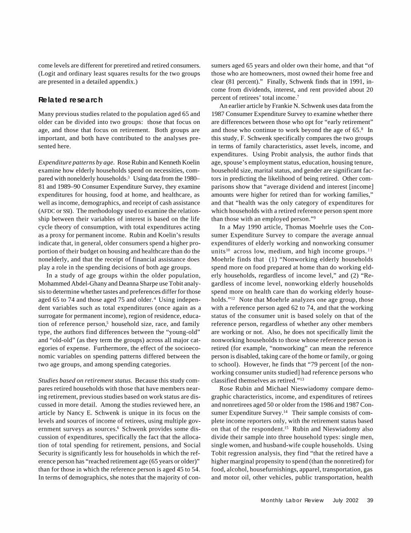
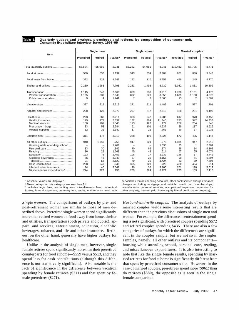
In general, the results indicate that the preretired and re-tired households do spend differently, across all family typesexamined. (See table 3.) For the majority of spending catego-ries within each household type (single male, single female,and married couple), the differences are statistically signifi-cant. In fact, the following categories are significant for allthree groups: total quarterly outlays, food away from home,shelter and utilities, total transportation, private transporta-tion, apparel and services, total healthcare, health insurance,prescription drugs, education, alcoholic beverages, tobacco,and life and other insurance. Many of these differences areeasily intuited: for instance, one expects significant differ-ences in total outlays due to the significant differences intotal income (as measured by income before taxes). Also,

given the homeownership rates and mortgage status com-parisons, it is not surprising that preretired consumer unitsspend more than retirees on shelter and utilities. Additionally,private transportation (expenses for the consumer unit’sowned vehicles) is significantly higher for preretired singlesand couples than for retirees. Even though the sample hasbeen restricted to those households who own at least onevehicle, retirees may have paid off their vehicles, and mayhave lower maintenance and gasoline expenditures due toless use of the vehicle than preretirees, who may be driving towork every weekday.

Single men. Preretired single men spend more overall($6,804)—and for most categories of interest—than do singlemale retirees ($5,050 total quarterly outlays). The only excep-tions are healthcare, for which retirees spend almost twice asmuch ($560) as the preretired households spend ($293), andcash contributions, for which retired men spend $649 com-pared with $268 spent by preretirees. Within the category ofhealthcare, outlays are higher by retirees for each compo-nent, but are only significantly so for insurance and prescrip-tion drugs.

Interestingly, expenditures for food at home are not sig-nificantly different for retired and preretired single men,but preretirees spend significantly more for food away fromhome ($372) than retired single men spend ($224). Con-comitantly, retired single men (73 percent) report food-away-from-home purchases less frequently than preretirees(90 percent). Thus, even the average expenditure for re-tired single men who purchase food away from home issubstantially smaller ($305) than the average expenditurefor similar preretired single men ($415).26 The most obvi-ous explanation is, once again, the difference in income forthese groups. But perhaps this is a mobility issue, as retir-ees are older and may have health-related barriers to goingout. This would seem to be supported by their signifi-cantly smaller outlays for vacations and trips, contrary tothe proposed notion of increased leisure and travel afterretirement. Furthermore, retirees spend significantly lesson entertainment items and services ($178) than dopreretirees ($311)—entertainment expenditures also includesome items related to mobility, such as tickets to sportingand cultural events (theater, concerts, and so forth).

Outlays for apparel and services are also significantlylower in the post-retirement single male households: $123compared with $208 spent by preretirees. Presumably, atleast part of the preretired male’s purchases will be forwork clothing, a cost no longer applicable to the retirees.Also, deductions for employer-sponsored plans may ac-count for some of the relatively higher outlays for life in-surance by the preretired sample—$94 compared with $40spent by retired single men.


Table 3. Quarterly outlays and t-values, preretirees and retirees, by composition of consumer unit,Consumer Expenditure Interview Survey, 1998–99

Item

Total quarterly outlays ....................... $6,804 $5,050 2.941 $6,222 $4,911 3.941 $10,482 $7,705 8.471

Food at home ................................ 580 536 1.139 513 559 2.384 961 880 3.448

Food away from home ..................... 372 224 4.249 182 110 6.357 449 245 5.770

Shelter and utilities ........................ 2,250 1,286 7.795 2,283 1,496 6.730 3,082 1,831 10.592

Transportation ............................... 1,145 643 2.666 809 530 3.916 1,700 1,131 4.478Private transportation .................. 1,135 639 2.640 802 528 3.855 1,685 1,130 4.373Public transportation .................... 9 4 1.241 7 2 2.565 15 2 5.682

Vacation/trips ................................ 387 212 2.219 271 211 1.485 623 577 .791

Apparel and services ...................... 208 123 2.973 297 217 2.613 428 231 9.195

Healthcare .................................... 293 560 3.214 333 542 6.986 617 970 8.453Health insurance ......................... 149 271 5.337 132 294 11.340 293 542 14.735Medical services ......................... 100 201 1.340 123 127 .177 206 204 .046Prescription drugs ....................... 33 58 2.284 61 101 4.537 89 187 8.626Medical supplies ......................... 12 31 1.140 17 21 .765 30 37 1.033

Entertainment ................................ 311 178 3.910 238 196 2.325 572 435 1.146

All other outlays ............................ 940 1,050 .255 917 721 .976 1,331 947 2.915Housing while attending school2 .... – – 1.409 – – 1.635 25 1 2.881Personal care ............................. 33 30 .845 70 65 .874 98 84 4.169Reading ..................................... 36 28 1.661 45 43 .514 67 55 4.074Education ................................... 123 6 2.453 108 17 2.239 155 17 3.742Alcoholic beverages .................... 86 46 3.347 37 20 3.156 90 51 6.394Tobacco ..................................... 91 58 2.622 49 30 3.424 83 39 7.795Cash contibutions ....................... 268 649 .948 365 328 .220 428 484 .514Life and other insurance .............. 94 40 3.649 79 36 3.266 201 120 5.517Miiscellaneous expenditures 3 ........ 244 222 .253 209 224 0.221 275 153 2.110

1 Absolute values are displayed.2 Mean outlays for this category are less than $1.3 Includes legal fees; accounting fees; miscellaneous fees, parimutuellosses; funeral expenses; cemetery lots, vaults, maintenance fees; safe



deposit box rental; checking accounts, other bank service charges; financecharges excluding mortgage and vehicle; credit card memberships;miscellaneous personal services; occupational expenses; expenses forother property; interest paid, home equity line of credit (other property);

Single women. The comparisons of outlays by pre- andpost-retirement women are similar to those of men de-scribed above. Preretired single women spend significantlymore than retired women on food away from home, shelterand utilities, transportation (both private and public), ap-parel and services, entertainment, education, alcoholicbeverages, tobacco, and life and other insurance. Retir-ees, on the other hand, generally have higher outlays forhealthcare.

Unlike in the analysis of single men, however, singlefemale retirees spend significantly more than their preretiredcounterparts for food at home—$559 versus $513, and theyspend less for cash contributions (although this differ-ence is not statistically significant). Also notable is thelack of significance in the difference between vacationspending by female retirees ($211) and that spent by fe-male preretirees ($271).

Husband-and-wife couples. The analysis of outlays bymarried couples yields some interesting results that aredifferent than the previous discussions of single men andwomen. For example, the difference in entertainment spend-ing is not significant, with preretired couples spending $572and retired couples spending $435. There are also a fewcategories of outlays for which the differences are signifi-cant in the couples sample, but are not so in the singlessamples, namely, all other outlays and its components—housing while attending school, personal care, reading,and miscellaneous expenditures. It is also interesting tonote that like the single female results, spending by mar-ried retirees for food at home is significantly different fromthat spent by preretired consumer units. However, in thecase of married couples, preretirees spend more ($961) thando retirees ($880), the opposite as is seen in the singlefemale comparison.



Regression analysis and results

Thus far, the results presented have examined differencesbetween the preretired and retired groups in general ways.For example, retirees may spend differently on certain goodsor services than might preretirees. But how much of this ef-fect is due to the lifestyle differences (such as additional freetime) that accompany retirement, and how much is due toother differences, such as lower income or other factors? Tohelp discern the effect that retirement has, regression analy-sis is useful.

In this study, two types of regressions are performed: lo-gistic regressions, or “logits,” and ordinary least squares (OLS)regressions.27 Each has a different purpose. The logits areused to ascertain the probability that an event (such as aparticular expenditure) will occur, given characteristics of theconsumer unit. The logits are only necessary for expendi-tures that are not universally made. The OLS regressions de-scribe how expenditure levels are related to certain character-istics. (For example, most expenditures are expected to in-crease with income, but by how much?) Table 4 shows thepercent reporting expenditures that are used for regressionanalysis, and table 5 shows the number of observations usedfor ordinary least squares regressions.

The expenditures selected for study are either those thatare basic goods and services (food at home, shelter and utili-ties, apparel and services, healthcare less insurance, andtransportation) or items that might be expected a priori todiffer with retirement (food away from home, entertainment,and out-of-town trips) due to the increased availability of lei-sure time. All categories are examined using OLS. Of the basicgoods, only apparel and services requires a logit analysis.However, the “leisure” expenditures all require logit analysis.

Healthcare is the one basic expenditure group that requiresspecial consideration. Only the “out-of-pocket” expendituresfor actual medical goods and services are examined, becausethe quality of health insurance coverage can differ so muchfor these groups. Presumably, all the retirees in our sample areeligible for Medicare coverage. This is not true of thepreretirees. Thus, the utility of comparing probability of cov-erage is limited. However, even if one only examines expendi-tures for actual drugs, medical supplies, and services, the re-sults are still unclear: if the expenditures for “noninsurance”healthcare are higher for retirees, is this due to health reasons,or to less adequate coverage? The analysis in this study shallnot attempt to answer these questions; even so, becausehealthcare is an important factor in maintaining quality of life,the results are reported for those who may find its inclusionuseful (such as those who only want to see the “bottomline”—that is, the expected difference in spending associatedwith retirement, whatever the reason may be).

The independent variables for each of the regression mod-els are similar. For the logistic regressions, the independentvariables used describe occupation of the reference person(retired or preretired, self-employed); marital status for singles(divorced, separated, or never married); race (black) andethnicity (Hispanic) of the reference person; educational at-tainment of the reference person (high school graduate, somecollege, college graduate, attended graduate school); degreeof urbanization for the consumer unit (that is, urban or rurallocation); region of residence of the consumer unit; housingtenure (home owned without mortgage or renter); and totaloutlays that are used as a proxy for “permanent” income.(Also, an interaction term is included to see if the relationshipof expenditure to “permanent” income differs in retirement.)This study uses “permanent” instead of “current” (that is,

Table 4.

Food at home .............................. 99.2 100.0 99.8 99.9 99.9 99.9Food away from home .................. 89.6 73.4 80.1 73.1 89.4 80.7Shelter and utilities (owners) ......... 100.0 100.0 100.0 100.0 100.0 100.0Shelter and utilities (renters) ......... 100.0 100.0 100.0 100.0 99.0 100.0Apparel and services ................... 81.5 68.5 86.3 77.0 88.3 79.5Healthcare less insurance1 ........... 49.6 60.4 73.1 75.0 80.1 84.8Transportation ............................. 98.9 98.7 99.8 97.7 99.6 99.5Entertainment .............................. 89.6 73.9 88.1 84.7 95.3 90.8Out-of-town trips ......................... 40.8 32.4 41.7 36.4 55.6 48.0

Percent reporting expenditures that are analyzed using regression analysis

Outlay category

NOTE: These figures are calculated from the full sample. Therefore,the values for percent reporting may differ slightly from thoseobservations actually used in the regression. Missing values for someindependent variables cause a few observations to be removed fromthe regressions, as described in the main text.

1 Percent reporting positive values only. Those reporting netreimbursements—that is, negative values—and those reporting no

expenditure are treated as “nonexpenditures.” Reimbursements are rare,however. The largest percentage occurs for retired single males, and accountsfor 3.6 percent of the group. Reimbursements are reported for 1.5 percent ofpreretired single males, and 1.4 percent of preretired married couples. For allothers, reimbursements account for percentages greater than 0.9 but lessthan 1.0 percent.


Preretired Retired Preretired PreretiredRetired Retired


annual) income because, according to the “permanent incomehypothesis,” expenditures are often made with expectationsof future earnings in mind.28 In this study, it is particularlyimportant to use “permanent income” as opposed to “currentincome,” because table 2 shows current income is vastly dif-ferent for the preretired and retired groups. This is becausethe retiree by definition has ceased working, and so he or shemust live off of savings and other assets that have been accu-mulated. Any income received will presumably be based onthese assets (such as interest or dividends), or will be fromsome source related to previous labor (such as Social Securityor pension income). Even so, these income sources by them-selves may not be enough to sustain a comfortable living situ-ation for most consumers (retired or otherwise), and would bean unrealistic measure of the consumer unit’s actual economicstatus.29 Expenditures reflect rational decisions based on lev-els of wealth (rather than income alone) that are available tothe consumer unit, and therefore serve as a better indicator ofthe consumer unit’s tastes and preferences for particular goodsand services. (Additionally, by using “permanent income”instead of “current income,” there is no need to distinguish“complete” and “incomplete” reporters, as virtually all respon-dents provide some information on outlays.)

The purpose of regressions, as noted earlier, is to allow“ceteris paribus” comparisons. That is, given that two con-sumer units are identical except for the issue in question (inthis case, retirement), how does this issue influence the ex-pected outcome for the affected consumer? To aid compari-sons, a control group is selected, and its characteristics areused with the regression coefficients to predict the outcomesfor each consumer unit (that is, preretired or retired). In thisstudy, the control group consists of consumer units who are:currently working for a wage or salary; widowed (if single);neither black nor Hispanic; lacking a high school degree; liv-ing in an urban area of the South; and homeowners with amortgage. In a few of the OLS regressions, additional controlsare applied. For example, it is assumed that single homeowners

live in a dwelling with six rooms (including bedrooms) and twobathrooms (including half baths), compared to four rooms andone bathroom for single renters. For couples, owners are as-sumed to have seven rooms and two bathrooms, while rentersare assumed to have five rooms and one bathroom. It is alsoassumed for all consumer units that they own one automobileand no other vehicles. These characteristics play roles indifferent models; for example, outlays for shelter and utilitieswill obviously vary with the size of the dwelling; transporta-tion outlays will depend on number of vehicles owned (auto-mobile or otherwise). Some other outlays, such as entertain-ment, may also depend on numbers of vehicles. One enter-tainment expenditure category specifically accounts for ex-penditures on vehicles like boats or motorcycles. In somecases, the consumer unit owns these vehicles (such as a boat)specifically for recreational purposes; in other cases, havingaccess to certain vehicles (such as motorcycles) may makeaccess to certain areas a greater possibility, and the opportu-nity may drive the expenditure.

Also, before performing the regressions, all expenditurevalues (including permanent income) were transformed by tak-ing their natural log. This was done to minimizeheteroscedasticity, which can be a problem in regression mod-els. However, it has a convenient side-effect in that the mar-ginal propensities to consume (MPC) and income elasticitieshave special properties: For all the basic goods (except ap-parel and services), the MPC becomes proportional to the ex-pected budget share for the item under study; the elasticitiessimply equal the coefficient on natural log of permanent in-come. (For more information, see the appendix.)

Before examining the results, two caveats are in order: First,for the “ceteris paribus” analysis, note that average total out-lays are used as the “control” amount, and that the averagefor preretired consumers is the operative value. This may notseem realistic, since the tables clearly show that outlays de-cline with retirement. There are several reasons for this: Evenif tastes and preferences do not change in retirement, retireesare more likely to have paid off their mortgage, which wouldsubstantially reduce outlays. Additionally, as noted earlier,because the Consumer Expenditure Survey is not longitudi-nal, it is impossible to obtain a large sample whereby the act ofretirement may be observed, let alone one where several years(or at least time periods) of expenditures both prior to and afterretirement may be observed. Given the method used to definethe sample, then, it could be that some selection bias is intro-duced into the data; that is, perhaps a substantial amount ofthe “preretirees” are consumers who plan to continue to workduring retirement, though not necessarily at their original ca-reer job. These consumers may have different characteristics(including tastes) than those who retire completely, and thusthey “select” themselves out of the retiree sample. However,assuming this problem is minimal, the issue still remains that

Outlay Single Single Marriedcategory men women couples

Food at home ................................ 480 1,270 2,542Food away from home .................... 396 968 2,168Shelter and utilities (owners) ........... 317 985 2,354Shelter and utilities (renters) ........... 160 279 153Apparel and services ..................... 364 1,030 2,139Healthcare, less insurance ............. 263 944 2,096Transportation ............................... 476 1,254 2,532Entertainment ................................ 397 1,096 2,370Out-of-town trips ........................... 161 467 1,206

Table 5. Number of observations for ordinary leastsquares regressions

NOTE: The married couple regressions are missing one observation dueto one negative observation for permanent income; presumably, this couplehad a relatively large reimbursement for healthcare that overwhelmed theirother expenditures in the quarter in which it was received.



expenditures decline in retirement for those in the sample. The“ceteris paribus” results are concerned with the effect of theretirement decision itself, so in this discussion there is noproblem. (See tables 6 and 7.) However, some readers may beinterested in learning how expenditures differ in reality as atotal result of retirement and its concomitant decisions thatresult in lower total outlays. For that purpose, tables are in-cluded in Appendix A that show the “total effect” of retire-ment. (That is, most characteristics, such as region of resi-dence, are held constant, but permanent income is allowed todecrease.)

Second, one other factor cannot be separated out from theretirement decision: by definition, the retirees in this sampleare older than the preretirees. Therefore, some of the retire-ment effect may be increased or decreased by an age effect.(This may be especially true for an expenditure such ashealthcare less insurance.)

Finally, the number of observations differs from the fullsample size in a few cases. This is generally due to missingdata; for example, occasionally a consumer unit does not pro-vide information on number of rooms or bathrooms in thehousehold, and those records are deleted from the regres-sion. Also, in the case of healthcare less insurance, the ex-penditure can be reported as negative because of reimburse-ments made by insurance companies. If a consumer unitmade an expenditure for healthcare in one quarter and re-ceived reimbursement in a subsequent quarter, the healthcareexpenditure during the “reimbursement” quarter will appearas a negative value. Although on average the reimburse-ments and the expenditures will cancel each other out, in the

regression results they can be problematic.30 Fortunately,these occurrences are infrequent.

Table 5 shows the total number of observations used inthe OLS regressions.31 For apparel and services and the “lei-sure” regressions, observations are less than the total samplesize because only those who had positive outlays are includedin the OLS stage, as explained in the appendix.

Single men. In the case of single men, retirement status ap-pears to play an indirect role in expenditure patterns. AlthoughMPCs and elasticities appear to differ in several of the “basic”goods cases, none of these is associated with a statisticallysignificant retirement effect, either for retirement in general orfor the interaction of retirement and income, except for trans-portation. In this case, the predicted expenditure is signifi-cantly related both to the “event” of retirement and to a changein the income/expenditure relationship. Outlays are predictedto drop significantly both in economic and statistical terms.(The difference is $265 per quarter.) The MPC declines sub-stantially—from less than $0.18 to more than $0.09. The de-crease in elasticity indicates that this good falls from “luxury”status for preretirees to “necessity” status for retirees. Thismay indicate that before retirement, single men, if given moreincome, will buy vehicles more frequently or more expensivevehicles than they would upon retirement. Again, retireesmay also have less need to drive (therefore, they pay less forgasoline and other travel expenditures), as they do not haveto go to work every day. (Note that single women and marriedcouples also experience declines in predicted expenditures fortransportation in retirement, although in those cases the dif-

Table 6.

Single men:Food away from home ................... 94.6 93.0 (1) –Apparel and services .................... 60.6 70.3 – –Healthcare .................................. 39.8 71.6 – –Entertainment .............................. 90.7 88.2 – –Out-of-town trips .......................... 33.2 29.6 – –

Single women:Food away from home ................... 81.4 83.6 – –Apparel and services .................... 82.0 74.1 – –Healthcare .................................. 84.2 87.8 – –Entertainment .............................. 92.8 90.2 – –Out-of-town trips .......................... 33.8 27.5 – –

Married couples:Food away from home ................... 92.7 86.9 – –Apparel and services .................... 90.5 85.6 – –Healthcare .................................. 89.1 93.4 – –Entertainment .............................. 96.7 93.8 – –Out-of-town trips .......................... 45.4 46.6 – –

Predicted probabilities, “ceteris paribus”[In percent]

Significance indicatorCeteris paribus criteria

Probability of purchase

Preretired Retired Retirement Income

1 Significant at the 95-percent confidence level.Dash indicates result not significant at the 95-percent confidence level.

ference is not statistically significant.)As for the “leisure” goods tested,

two show a difference related to theprobability of purchase. In the firstcase, food away from home, the over-all difference in predicted probabilityis not meaningful—falling from lessthan 95 percent for preretirees to 93percent for retirees; the bottom line ismost single men are predicted to pur-chase food away from home at leastonce every few months in retirement.Nor is the effect on MPC meaningful;it remains under $0.02 regardless of re-tirement status. However, for out-of-town trips, the results are more inter-esting. The probability of purchasedeclines 3 percentage points, dueboth to the retirement effect and a dif-ference in the income/probability rela-tionship after retirement. The pre-dicted expenditure for actual buyers


Variables:Permanent income ............................. $6,804 $6,804 $6,222 $6,222 $10,482 $10,482Log income ....................................... 8.825266 8.825266 8.735847 8.735847 9.257415 9.257415

Owners:Rooms/bedrooms ............................... 6 6 6 6 7 7Bathrooms/halfbaths .......................... 2 2 2 2 2 2

Renters:Rooms/bedrooms ............................... 4 4 4 4 5 5Bathrooms/halfbaths .......................... 1 1 1 1 1 1

Food at home:Probability of purchase ....................... 100.0 100.0 100.0 100.0 100.0 100.0Predicted expenditure (buyers only) ..... $536 $503 $470 1,2$546 $897 $878Marginal propensity to consume ........... .014 .024 .019 .034 .020 .022Elasticity .......................................... .18 .32 .26 .39 .24 .27

Food away from home:Probability of purchase ....................... 94.6 193.0 81.4 83.6 92.7 86.9Predicted expenditure (buyers only) ...... $193 $162 $169 $119 $305 1,2$252Marginal propensity to consume ........... .013 .015 .017 .012 .022 .014Elasticity ........................................... .45 .65 .64 .63 .76 .57

Shelter and utilities (owners):Probability of purchase ....................... 100.0 100.0 100.0 100.0 100.0 100.0Predicted expenditure (buyers only) ..... $2,509 $2,005 $2,185 $1,947 $3,090 $2,972Marginal propensity to consume ........... .216 .137 .246 .206 .166 .148Elasticity .......................................... .59 .46 .70 .66 .56 .52

Shelter and utilities (renters):Probability of purchase ....................... 100.0 100.0 100.0 100.0 100.0 100.0Predicted expenditure (buyers only) ..... $1,523 $1,769 $2,088 $1,923 $1,992 $1,570Marginal propensity to consume ........... .096 .147 .240 .248 .103 .068Elasticity .......................................... .43 .57 .71 .80 .54 .45

Apparel and services:Probability of purchase ....................... 60.6 70.3 82.0 74.1 90.5 85.6Predicted expenditure (buyers only) ..... $111 $99 $142 2$99 $253 1,2$183Marginal propensity to consume ........... .012 .013 .024 .013 .024 .015Elasticity .......................................... .73 .92 1.08 .83 1.00 .83

Healthcare (less insurance):Probability of purchase ....................... 39.8 71.6 84.2 87.8 89.1 93.4Predicted expenditure (buyers only) ..... $226 $370 $158 1,2$218 $228 $336Marginal propensity to consume ........... .012 .045 .014 .033 .016 .020Elasticity .......................................... .35 .82 .55 .95 .72 .61

Transportation:Probability of purchase ....................... 100.0 100.0 100.0 100.0 100.0 100.0Predicted expenditure (buyers only) ..... $1,018 1,2$753 $476 $373 $1,197 $889Marginal propensity to consume ........... .175 .094 .052 .043 .110 .083Elasticity .......................................... 1.17 .85 .68 .71 .96 .98

Entertainment:Probability of purchase ....................... 90.7 88.2 92.8 90.2 96.7 93.8Predicted expenditure (buyers only) ..... $188 $155 $139 $134 $284 $236Marginal propensity to consume ........... .021 .014 .015 .015 .026 .021Elasticity .......................................... .76 .63 .67 .69 .95 .91

Out-of-town trips:Probability of purchase ....................... 33.2 29.6 33.8 27.5 45.4 46.6Predicted expenditure (buyers only) ..... $98 $96 $157 1,2$155 $435 $530Marginal propensity to consume ........... .012 .006 .012 .012 .030 .047Elasticity .......................................... .82 .43 .48 .49 .73 .92

Table 7. Elasticities, and so forth under “ceteris paribus”

[Probabilities in percent]

Ceteris paribus criteriaSingle men Single women Married couples

Preretired Retired Preretired PreretiredRetired Retired

1 Retirement coefficient is statistically significant at the 95-percent confidence level.2 Coefficient for retired income term is statistically significant at the 95-percent confidence level.



does not differ much, but the MPC is cut in half—from $0.012to $0.006, as is the income elasticity—from 0.82 to 0.43.32

Single women. The probabilities of purchase are not signifi-cantly affected by retirement for single women, according tothe logit results. However, in several cases, retirement is di-rectly and indirectly related to differences in expenditures forthose who purchase. Food at home, healthcare (less insur-ance), and out-of-town trips all exhibit such differences, andapparel and services exhibits an indirect difference (that is,the income coefficient is statistically significant, but not theretirement variable itself). For food at home, a sizable increasein expenditures is predicted—about $76 per quarter. Althoughnot statistically significant, food away from home also showsa decline in predicted expenditure for single female retirees($50). It is interesting to note that the table in the appendix, inwhich retirees are assumed to have lower permanent incomesthan preretirees, shows that the situation reverses. Althoughfood-at-home expenditures are predicted to rise (by $28), thedifference is less than the predicted decrease in food-away-from-home expenditures ($65).

An interesting difference occurs for apparel and servicesfor this group. After retirement, the MPC for this item is cut inhalf. As a result, the elasticity falls substantially as well. Be-fore retirement, apparel and services are treated as “luxury”goods for single women; afterward, they become “necessity”goods, although they still have a higher elasticity than mostof the other expenditure items. It is also interesting to notethat although preretired single women are predicted to spendmore ($142) than preretired single men ($111) each quarter,male and female retirees have the same predicted expenditure($99) for apparel and services. This is also roughly true whenincomes are assumed to decline for retirees—both single maleand female retirees are predicted to spend about $80 on ap-parel and services. (See appendix.)

Married couples. As with singles, married couples appearto have some substantial differences either in probabilityof purchase or level of purchase, but not many are statisti-cally significant. The only two expenditures that showsignificant differences are food away from home and ap-parel and services. Both show decreases in the predictedexpenditure due to the direct retirement effect and changesin the income effect. The apparent difference in probabil-ity for food away from home is the largest of the threegroups studied, falling nearly 13 percentage points. Simi-larly, the expenditure for those who report purchases fallsby $85 per quarter. Nevertheless, the difference in MPC isnot even noticed when rounded to the full cent (that is,$0.02 before and after retirement). The elasticity declinessomewhat, from 0.76 to 0.62, but still remains in the moder-ately high level of inelastic expenditures.

Apparel and services, though, show a pattern very similarto single women. Although all groups show declines in pre-dicted expenditures, probably because of less need for workattire or uniforms as noted before, apparel and services fallfrom unitary elasticity for preretired couples to inelasticity(0.83) for retirees. The MPC is also substantially reduced (from$0.024 to $0.015). Predicted expenditures fall by $70 for thisgroup.

THIS STUDY HAS ANALYZED EXPENDITURE PATTERNS BY PRERETIREES

AND RETIREES to help understand how expenditure patternsdiffer upon retirement for single men, single women, and mar-ried couples. Many differences have been found. Some ofthese are undoubtedly due to differences that are to be ex-pected upon retirement. For example, retirees have lower in-comes than preretirees, and therefore would naturally be ex-pected to spend less on many items. However, preretirees arefound to have different demographic characteristics than re-tirees, even when examining carefully selected groups (singlemen, single women, and married couples with no children).Again, some of these are expected; age is by definition greaterfor retirees than preretirees, and retirees are more likely to owntheir home outright (that is, the mortgage is paid off) than arepreretirees. Others are not necessarily predictable a priori,such as differences in proportions of each group that are lo-cated in various regions of the country. Nevertheless, each ofthese characteristics could have an effect on expenditure pat-terns. To control for these differences, and to attempt to as-certain whether income differences are solely responsible forexpenditure differences or whether tastes and preferences dif-fer in retirement, regression analyses are performed.

From the regression results, it is difficult to draw generalconclusions about the role of retirement in expenditure deci-sions. For example, the results for single men showed fewstatistically significant differences in probability of reportingexpenditures or in the predicted outlay for items. However,more were significant for single women and married couples.Nevertheless, some interesting findings are presented. Forexample, in each group studied, both the probability of pur-chase and predicted expenditure for food away from home arelower for retirees than preretirees. Because these results arecalculated assuming income is equal for the pre- and post-retirees, it may indicate that the “utilitarian” purpose of foodaway from home outweighs the “recreational” purpose of foodaway from home. That is, the preretirees may be purchasingmore food away from home more frequently because they donot have the same amount of leisure time as the retirees. How-ever, given the lack of statistical significance of many of theparameters used to compute these results, this interpretationshould be viewed with caution.

Retirement is a major event in a working person’s life,accompanied by many lifestyle changes, such as a reduc-


tion in labor income and an increase in leisure time. Thisarticle documents some of the potential consequences ofthese changes. These issues are particularly importanttoday with the “graying” of the population; it is only a fewyears until the “baby boomers” reach retirement age. This

analysis should be useful not only to professionals andpolicymakers who study the effects of changing demo-graphics on the economy at large, but also to retirementplanners and counselors, as well as to those who plan toretire soon themselves.

Notes

NOTE: Additional tables can be obtained on the Internet version of thisarticle at http://www.bls.gov/cex/csxart.htm

1 See 65+ in the United States, Current Population Reports, SpecialStudies (U.S. Bureau of the Census, 1996), pp 23–190.2 Geoffrey D. Paulin, “Expenditure patterns of older Americans, 1984–97,” Monthly Labor Review, May 2000, pp. 3–28.3 Rose M. Rubin and Kenneth Koelin, “Elderly and nonelderly expen-ditures on necessities in the 1980s,” Monthly Labor Review, September1996, pp. 24–31.4 Mohammed Abdel-Ghany and Deanna L. Sharpe, “Consumption Pat-terns Among the Young-Old and Old-Old,” Journal of Consumer Af-fairs, Summer 1997, pp. 90–112.5 The reference person is the first person mentioned by the surveyrespondent when asked: “Start with the name of the person or one ofthe persons who owns or rents this home.”6 Nancy E. Schwenk, “Trends in the Economic Status of RetiredPeople,” Family Economic Review, 1994, 7(2), pp. 19–27.7 Ibid., pp. 24–25.8 Frankie N. Schwenk, “A Comparison of Households Headed by Per-sons 55 to 65 Years of Age: Retired and Employed,” Family EconomicReview, 1990, 3(3), pp. 19–25.9 Ibid., pp. 22, 24.10 A consumer unit is defined as members of a household related byblood, marriage, adoption, or other legal arrangement; a single personliving alone or sharing a household with others but who is financiallyindependent; or two or more persons living together who share respon-sibility for at least two out of three major types of expenses—food,housing, and other expenses. In this article, consumer unit and house-hold are used interchangeably.11 Thomas Moehrle, “Expenditure patterns of the elderly: workers andnonworkers,” Monthly Labor Review, May 1990, pp. 34–41.12 Ibid., p. 34.13 Ibid., p. 36.14 Rose M. Rubin and Michael Nieswiadomy, “Expenditure patterns ofretired and nonretired persons,” Monthly Labor Review, April 1994, pp.10–21.15 A complete income reporter is a consumer unit that provides valuesfor at least one of the major sources of its income, such as wages andsalaries, self-employment income, and Social Security income. A com-plete reporter may not provide a full accounting of all income from allsources, however.16 Rubin and Nieswiadomy, “Expenditure patterns…,” p. 36.17 The 1996–97 Consumer Expenditure Survey 2-year report notesthat the “Interview survey collects detailed data on an estimated 60 to70 percent of total household expenditures. In addition, global esti-mates—that is, expense patterns for a 3-month period—are obtainedfor food and other select items. These global estimates account for anadditional 20 to 25 percent of total expenditures.” Source: Bureau ofLabor Statistics, Consumer Expenditure Survey, 1996–97, Report 935(U.S. Department of Labor, September 1999), p. 256.18 It is important to note that some retirees in our sample may be“retired due to disability.” However, in the Consumer Expenditure Sur-vey, there is no way to identify those who are both retired and disabled.

Respondents may select only one of the categories—“retired” or “notworking due to disability.”19 The other possible occupational statuses for the spouse are “workingwithout pay” or “not working” because they are either going to schoolor doing something else (that is, not working for a reason not alreadydescribed).20 Beth Harrison highlights the differences in expenditure levels andshares between these two age groups from the 1984 Consumer Expen-diture Interview Survey, finding them to be distinct in most majorcategories. (See “Spending patterns of older persons revealed in expen-diture survey,” Monthly Labor Review, October 1986, p. 15–17.) Inaddition, in a study following up on Harrison’s findings, Pamela Hitschler(p. 3) finds that “consumer units in the younger group spent, on aver-age, a significantly larger amount on every major expenditure categoryexcept housing and healthcare in both years [1980 and 1990 are com-pared].” (“Spending by older consumers: 1980 and 1990 compared,”Monthly Labor Review, May 1993, pp. 3–13.)21 This “age effect” is assumed to include differences by age in healthstatus. Although health status can be an important influence on theexpenditures of older consumers, there are no concrete measures ofhealth status available in the Consumer Expenditure Survey.22 As described previously, the definition of “preretired” and “retired”depends on the occupational status of the reference person and spouse,in the case of married couples. It is possible that one of the parentsowns the home, and is therefore the reference person, but the childmoves back in with them to provide economic support.23 Even eliminating families with children does not guarantee that thecouple is childless. College students, when living in university-spon-sored housing, are considered to be separate consumer units from theirparents. Additionally, children may have reached the age of majority,and may have moved out to establish consumer units of their own.However, the survey does not collect information in such a way as toallow the selection of singles or couples who do not have children at all.Therefore, although it is possible that some of these families purchaseitems for their children that those without children would not, it is notpossible to identify those families with the possibility of such additionalspending.24 Recall that the definition of retirement in this study is based on theself-reported occupation of the reference person. Thus, it is possible toretire from one’s life-long work and to pursue other avenues of em-ployment. The “retiree” may choose to work for pay in a field thatwas previously a hobby, or perhaps may seek a low-wage job to keepactive, but not for income, per se.25 While it is true that some “expenditures,” such as mortgage princi-pal, may be considered an “investment” in some cases, mosthomeowners do not own their home solely for investment purposes, asthey might a stock or bond; they also consume the housing services thehome provides. Similarly, some consumers may own life insurancepolicies that pay annuities at some point; however, the policy is notmerely a savings vehicle; it is primarily a purchase of protection ofone’s estate in case of unexpected events.26 Calculated by dividing the average expenditure for the whole group($372 for preretirees, and $224 for retirees) by the percent reporting,shown in table 6 (89.6 percent for preretirees, and 73.4 percent forretirees).27 See the Technical Notes section for a detailed explanation of theregression methodology, including the model specifications.



APPENDIX A: Results of regression analysis

In tables 6 and 7, results were shown assuming “ceteris paribus.” Thatis, all characteristics (including permanent income) except retirementwere assumed to be constant for the groups compared and the resultswere computed on that basis. In reality, permanent income declinessubstantially in retirement. For the reader’s convenience, the following

28 See Milton Friedman, A Theory of the Consumption Function(Princeton, NJ: Princeton University Press, 1957).29 There are also empirical reasons for using “permanent” income inthis case. Respondents do not always provide information on “cur-rent” income, and even those who do may not provide a full account-ing of all income from all sources. Furthermore, data regarding assetsand liabilities are only collected on a limited basis in the Interviewsurvey. However, the primary goal of the Interview Survey is tocollect expenditures.30 One possible solution is to use four complete quarters for eachconsumer unit, rather than treat each quarter independently as is donein this article. However, even this solution does not provide a bal-anced treatment of medical expenditures and reimbursements. Forexample, a reimbursement reported in the second interview (the firstinterview during which these data are collected) will have no matchingexpenditure because that expense would have been incurred by theconsumer unit prior to its participation in the survey. Likewise, amedical expenditure reported in the fifth and final interview may verywell be reimbursed afterward, when the consumer unit is no longer asurvey participant. There is no way to capture these prior expensesor future reimbursements.31 Because the logit models share the same specification, and becausethey predict the probability of an expenditure occurring, nearly all ofthem have the same number of observations as the sample size for thegroup under study. The exception is the set of healthcare less insur-ance models. The logit models have fewer observations than thesample for the group under study in this case, because the negative

healthcare outlays are omitted from the sample before running theregression. (For single men, the total is 470 observations; for singlewomen, it is 1,260 observations; and for married couples, it is 2,515observations.)32 At first glance, the predicted value for out-of-town trips may appearlow, but there are at least two reasons for this. First, out-of-town tripsare defined in the survey either as trips that last at least overnight forrecreation purposes, or “day trips” in which the participant travels atleast 75 miles from home. Therefore, they may be short in durationand not costly. Second, this phenomenon may be due to the economet-rics underlying the model. The specification may be inaccurate due toomitted variables, improper transformation of the dependent or inde-pendent variables, or other reasons. However, the standard errors ofthe relative coefficients are wide enough to encompass an extremelylarge range of predicted values. This is because, as noted, E(lnY) is thepredicted value resulting from the regression, and exp[E(lnY)] is thepredicted value for the expenditure. A very small deviation in E(lnY)can lead to a very large difference in exp[E(lnY)]. For example, asshown in the table, the current predicted value for preretirees is $98.This is based on E(lnY) of approximately 4.58. However, if E(lnY)increases by 1 to 5.58, exp[E(lnY)] increases to $265. Even at the 90-percent confidence level, an estimate of 5.58 is plausible; if all relevantparameters are evaluated at the lowest level in the 90-percent confi-dence interval, E(lnY) is approximately –3.88; if all are evaluated at thehighest level in the 90-percent confidence interval, E(lnY) is approxi-mately 12.99. The same reasoning applies to travel expenditures forsingle women. Applying the confidence intervals to their parametersyields an estimated range from 0.51 to 9.59 for E(lnY).

Table A-1. Probabilities of purchasing selected goods and services for preretired and retired consumers, allowing full retirement” effect, 1998–99

Single men:

Food away from home ......... 94.6 89.3 1 –Apparel and services .......... 60.6 57.3 – –Healthcare (less insurance) . 39.8 63.6 – –Entertainment .................... 90.7 83.2 – –Out-of-town trips ................ 33.2 23.7 – –

Single women:

Food away from home ......... 81.4 79.9 – –Apparel and services .......... 82.0 68.6 – –Healthcare (less insurance) . 84.2 86.1 – –Entertainment .................... 92.8 87.6 – –Out-of-town trips ................ 33.8 23.2 – –

Couples:

Food away from home ......... 92.7 80.1 – –Apparel and services .......... 90.5 77.9 – –Healthcare (less insurance) . 89.1 89.7 – –Entertainment .................... 96.7 89.3 – –Out-of-town trips ................ 45.4 34.9 – –

1 Significant at the 95-percent confidence level.Dash indicates result not significant at the 95-percent confidence level.

Probability of purchase Significance indicator

Pre-retired Retired Retirement Income

[In percent]

Consumer type

tables show the “full effect” of retirement as estimated from the regres-sions discussed in the text. Only characteristics that are not explicitlyrelated to retirement (such as whether one lives in an urban or rural area)are held constant. However, permanent income is evaluated at its meanfor retirees in the following calculations. (See tables A-1 and A-2.)


Variables: Permanent income ......................... $6,804 $5,050 $6,222 $4,911 $10,482 $7,705 Log income ................................... 8.825266 8.527144 8.735847 8.499233 9.257415 8.949625

Owners: Rooms/bedrooms ........................... 6 6 6 6 7 7 Bathrooms/halfbaths ...................... 2 2 2 2 2 2

Renters: .......................................... Rooms/bedrooms ........................... 4 4 4 4 5 5 Bathrooms/halfbaths ...................... 1 1 1 1 1 1

Food at home: Probability of purchase (percent) ..... 100.0 100.0 100.0 100.0 100.0 100.0 Predicted expenditure .................... $536 $457 $470 1,2 $498 $897 $809 Marginal propensity to consume ...... 0.014 0.029 0.019 0.040 0.020 0.028 Elasticity ....................................... 0.18 0.32 0.26 0.39 0.24 0.27

Food away from home: Probability of purchase (percent) ..... 94.6 2 89.3 81.4 79.9 92.7 80.1 Predicted expenditure (buyers only) . $193 $136 $169 $104 $305 1,2 $220 Marginal propensity to consume ...... 0.013 0.018 0.017 0.013 0.022 0.018 Elasticity ....................................... 0.45 0.68 0.64 0.63 0.76 0.62

Shelter and utilities (owners): Probability of purchase (percent) ..... 100.0 100.0 100.0 100.0 100.0 100.0 Predicted expenditure .................... $2,509 $1,746 $2,185 $1,666 $3,090 $2,531 Marginal propensity to consume ...... 0.216 0.161 0.246 0.223 0.166 0.171 Elasticity ....................................... 0.59 0.46 0.70 0.66 0.56 0.52

Shelter and utilities (renters): Probability of purchase (percent) ..... 100.0 100.0 100.0 100.0 100.0 100.0 Predicted expenditure .................... $1,523 $1,494 $2,088 $1,591 $1,992 $1,365 Marginal propensity to consume ...... 0.096 0.167 0.240 0.260 0.103 0.081 Elasticity ....................................... 0.43 0.57 0.71 0.80 0.54 0.45

Apparel and services: Probability of purchase (percent) ..... 60.6 57.3 82.0 68.6 90.5 77.9 Predicted expenditure (buyers only) . $111 $79 $142 2 $81 $253 1,2 $146 Marginal propensity to consume ...... 0.012 0.014 0.024 0.013 0.024 0.016 Elasticity ....................................... 0.73 0.89 1.08 0.81 1.00 0.86

Healthcare less insurance: Probability of purchase (percent) ..... 39.8 63.6 84.2 86.1 89.1 89.7 Predicted expenditure (buyers only) . $226 $292 $158 1,2 $172 $228 $284 Marginal propensity to consume ...... 0.012 0.046 0.014 0.033 0.016 0.023 Elasticity ....................................... 0.35 0.79 0.55 0.94 0.72 0.64

Transportation: Probability of purchase (percent) ..... 100.0 100.0 100.0 100.0 100.0 100.0 Predicted expenditure .................... $1,018 1,2 $584 $476 $316 $1,197 $659 Marginal propensity to consume ...... 0.175 0.098 0.052 0.046 0.110 0.083 Elasticity ....................................... 1.17 0.85 0.68 0.71 0.96 0.98

Entertainment: Probability of purchase (percent) ..... 90.7 83.2 92.8 87.6 96.7 89.3 Predicted expenditure (buyers only) . $188 $132 $139 $115 $284 $182 Marginal propensity to consume ...... 0.021 0.017 0.015 0.016 0.026 0.022 Elasticity ....................................... 0.76 0.65 0.67 0.69 0.95 0.95

Out-of-town trips: Probability of purchase (percent) ..... 33.2 1,2 23.7 33.8 23.2 45.4 34.9 Predicted expenditure (buyers only) . $98 $77 $157 1,2 $120 $435 $373 Marginal propensity to consume ...... 0.012 0.005 0.012 0.010 0.030 0.037 Elasticity ....................................... 0.82 0.35 0.48 0.42 0.73 0.76

1 Coefficient for retired income term is statistically significant at the 95-percent confidence level; retirement coefficient is statistically significant at the 95-percent confidence level.2 Retirement coefficient is statistically significant at the 95-percent confidence level.

Single men Single women Couples

Table A-2. Predicted outcomes given full retirement effect

Preretired Retired Preretired Retired Preretired RetiredVariables



APPENDIX B. Regression techniques

Some expenditures, such as food at home, or shelter and utilities, arereported by virtually all participants in the Consumer ExpenditureSurvey. For these items, the choice of regression technique is straight-forward: Ordinary least squares (OLS) suits them well. However,many expenditures are not universal. These purchases may not bemade because of tastes and preferences (for example, tobacco andsmoking supplies) or because of durability of the item (for example,vehicle purchases). In this study, four such variables are examined.Three (food away from home, entertainment, and out-of-town trips)are probably examples of the first situation (tastes and preferencesdissuade some consumers from purchase) while the fourth may be anexample of the second situation (perhaps the consumer had suffi-cient amounts of apparel during the last quarter, and did not needservices, such as dry cleaning or repair). These kinds of expendituresrequire special treatment in their analysis.

One set of models designed to handle these situations is called the“double hurdle” set of models. The set gets its name because theconsumer must first decide whether to purchase the item, and thenhow much to purchase. In these models, the hurdles are modeled intwo stages: stage one models the probability of purchase; and stagetwo models the level of purchase for those who buy the good. Re-sults of the two stages are used together to predict the expenditurefor a given consumer.

One popular form of double hurdle model is the Tobit model. Inthis model, the “hurdles” are estimated with the same independentvariables. The stages are estimated in such a way that one set ofparameter estimates is produced, and these parameters can be usedto estimate probability of purchase (using the cumulative densityfunction, as with probit) and the marginal propensity to consume (aswith OLS). The predicted expenditure is equivalent to the predictedexpenditure for those who purchase weighted by the probability ofpurchase.1 However, a major drawback of Tobit is the restrictions itmakes on the results. First, because one set of independent variablesis used, the model is only useful when the exact same set of variablespredicts both the probability of purchase and the level of expendi-ture. This is not always the case. For example, the probability ofpurchasing health insurance may depend on the size of one’s family.However, if a particular policy charges one premium for “family”coverage, regardless of the number of members of the family, theTobit model has a weakness in predicting expenditures for that policy.Furthermore, the Tobit model assumes that the “direction” of eachvariable is the same for the probability and for the level of consump-tion. This may not be true. For example, an article describing wineconsumption by U.S. men finds that those who have at least a highschool education are more likely to drink wine than men who havelower levels of education; however, they also find that men with atleast a high school education drink less wine than those who havelower levels of education.2

Other models have been proposed, however, to handle the “doublehurdle” situation. The models used in this study are based on a typedescribed by John G. Cragg.3 In Cragg’s method, the probability ofpurchase is estimated separately from the level of expenditures.Cragg’s approach has many advantages over the Tobit. The ability toseparate the probability of purchase and level of expenditure equa-tions allows differences in variables and signs across the two stagesof the analysis, providing Cragg’s approach with a “considerableinterpretational advantage” over the Tobit model, according toMohamed Abdel-Ghany and J. Lew Silver.4 Additionally, “Tobit …forces zero observations to represent corner solutions,” according toother researchers, who go on to discuss a weakness in Tobit already

addressed—namely, that it “presumes that the same set of variablesand parameter estimates determine both the discrete probability of anonzero outcome and the level of positive expenditures….”5

Although Cragg’s models use probit to predict the probability ofpurchase, he notes that logit can be used instead.6 Many standardeconometric textbooks point out that logit, when applied, producesprobability estimates that are nearly identical to probit estimates.However, logit is much easier to use and interpret. The equation forpredicting probability of purchase (P) is:

P = exp(a + bX)/[1 + exp(a + bX)]wherea is the intercept of the logit equationb is a vector of parameter estimatesX is a vector of independent variables.

The formula can be entered into a standard spreadsheet to estimateprobabilities of purchase for different consumers. Furthermore, theequation is easily differentiated to find the marginal relationship ofprobability to a particular variable. (For example, if income rises by$1, how much does the probability of purchase change?) With probit,an equation must be estimated, and the results must be looked up ina statistical table to find out the overall probability of an eventoccuring, as well as the marginal effect on probability from changinga variable.

In the version of the Cragg model used in this paper, the probabil-ity of purchase is estimated as suggested with a logistic regression.Separately, OLS is used to estimate expenditures for those who pur-chase the item.7 To get the final results, the predicted probability ofpurchase obtained from the first stage is multiplied by the predictedexpenditure for those who purchase. This essentially produces anaverage predicted expenditure, weighted by the probability of pur-chase. To illustrate the intuition behind obtaining this weighted aver-age predicted expenditure, suppose that a large sample of consumersis selected randomly. Suppose that 25 percent of the participantspurchased a particular item. Suppose that this item sold for $100.The average expenditure for all consumers is then $25, or 25 percentmultiplied by $100. If a smaller sample is randomly selected fromthis large group, the expected value of the average of that smallersample is also $25. This is because if a large number of randomsamples were pulled from the total sample, and each time the averageexpenditure was recorded, then the “grand average” (that is, the aver-age of the averages) is expected to be $25.

When estimating the marginal propensity to consume and elastic-ity for the Cragg models, the logit results are taken into account. Thisis because income is assumed to influence expenditures both directly(through level of expenditure) and indirectly (by changing the prob-ability of purchase). The mathematical details are provided in thefollowing sections (“Marginal Propensity to Consume (MPC)” and“Elasticities.”)

As a final point, there are some expenditures for which Tobit maybe appropriate, in that this technique assumes that, given enoughtime, all consumers will eventually purchase the given item. Forexample, less than 100 percent of all consumer units report expendi-tures for apparel and services every quarter, but given enough time, itis reasonable to assume that 100 percent will eventually purchasesome. However, Tobit still suffers the weaknesses described earlier,and for convenience, the Cragg model is used for all variables ana-lyzed in this study. Further examination of the Tobit model will beleft for future research.


Marginal Propensity to Consume (MPC). The marginal propensityto consume (MPC) is defined as the change in expenditure given aunit change in income. In this case, “permanent income” is the rel-evant variable for change.

The “OLS only” regressions described in the text (for food athome; shelter and utilities; and transportation) have the followingspecification:

E(lnY) = a + blnI + cXwhereE(lnY) is the predicted (or “expected”) value of the

dependent variablea is the interceptb is a parameter estimatelnI is the natural log of permanent incomecX represents all other independent variables multiplied

by their regression coefficients.

In this case, the MPC is calculated by finding the change in the pre-dicted expenditure given a $1 increase in permanent income, or∂E(Y)/∂I. Although the model is specified to calculate E(lnY), thedesired result is easily obtained:

∂E(lnY)/ ∂I = ∂(a + blnI + cX)/ ∂I1/[E(Y)]* ∂E(Y)/ ∂I = b*(1/I) = b/I∂E(Y)/ ∂I = b*[E(Y)/I]

This result has an interesting property in that the MPC is propor-tional to the budget share (that is, specific outlay divided by totaloutlays), with the proportion equal to the parameter estimate for lnI.

This still leaves one question: If the model predicts E(lnY), whatis E(Y)? This also is easily solved, in that:

E(Y) = exp[E(lnY)]

Using this formulation, one need only select a group of interest, usethe regression results to determine E(lnY), and then follow the proce-dures indicated. In this study, the “group of interest” is the controlgroup described in the text.

The Cragg-based models have a more complicated specification,but it is nevertheless solvable to yield the MPC. The MPC is stilldefined the same way and is still represented the same way math-ematically; that is,

MPC = ∂E(Y)/ ∂I.

However, the initial formulation is more complicated. The desiredresult is actually

E(Y) = P*exp[E(lnY)]where P is the probability of observing an expenditure.

To find ∂E(Y)/ ∂I, the product rule of calculus is used. That is:

∂E(Y)/ ∂I = P’exp[E(lnY)] + Pexp’[E(lnY)]

Recall that:

P = exp(α + βlnI + λX)/[1 + exp(α + βlnI + λX)])whereλX is a vector of all independent variables except income,each multiplied by their parameter estimates.

Therefore, to find P’, the quotient rule is used:

P’ = (f’g - fg’)/g2

wheref = exp(α + βlnI + λX)g = 1 + exp(α + βlnI + λX)f’ = g’ = (β/I)exp(α + βlnI + λX)

Because f’ and g’ are equal in this case, this simplifies algebraicallyto:

P’ = [f’(g – f)]/g2;

and, because g equals (f + 1), this reduces even further to:

P’ = [f’(f + 1 – f)]/g2 = f’/g2.

Now, with the much simplified result, it can be shown that:

P’ = [(β/I)exp(α + βlnI + λX)]/[1 + exp(α + βlnI + λX)]2.

Again, by substitution, this reduces to:

P*{[β/I]/[1 + exp(α + βlnI + λX)]}.

Therefore,

MPC = P*{[β/I]/[1 + exp(α + βlnI + λX)]}*exp[E(lnY)]+ Pexp’[E(lnY)];

exp’[E(lnY)] = exp[E(lnY)]*E’(lnY);exp[E(lnY)] = E(Y);E’(lnY) = ∂E(lnY)/∂I = 1/E(Y)*∂E(Y)/∂I

= 1/E(Y)*[b*E(Y)/I] = b/I;

Alternatively, because E(lnY) equals a + blnI + cX,

E’(lnY) = ∂E(lnY)/∂I = ∂(a + blnI + cX)/∂I = b*(1/I) = b/I;∴MPC = P*{[β/I]/[1 + exp(α + βlnI + λX)]}*E(Y) + P*[E(Y)*(b/I)];

orMPC = P*E(Y)*{[β/I]/[1 + exp(α + βlnI + λX)]} +

P*b[E(Y)/I]

Because the terms P and E(Y) are common to both pieces of thecomplicated right-hand side of this equation, mathematically, theMPC can be simplified by factoring these terms out, and multiplyingthem by the sum of the remaining pieces. However, the formula isleft in this form for the moment, to illustrate an intuitive point: Notethat the MPC is derived from the predicted value of the expenditurefor those who purchase as weighted by the probability of purchase.Note that the second term on the right-hand side, that is, P*b[E(Y)/I],is the same MPC as was found before, except that it is weighted by theprobability of purchase. The remaining term is a result of the factthat the predicted expenditure is affected indirectly because prob-ability of purchase changes as a result of income change.

Elasticities. Income elasticity (or more properly in this case, perma-nent income elasticity) is the percent change in expenditure for aspecific good (such as food at home) given a 1-percent increase in(permanent) income. For example, for retired single males, the in-come elasticity for food at home is estimated to be 0.32, meaning thatfor every 1-percent increase in permanent income, these men arepredicted to increase food-at-home expenditures by about one-thirdof 1 percent.



The equation for calculating elasticity (η) is:

η = MPC*I/E(Y)

In the case of the “ OLS only” regressions, the elasticity in this case isconstant, and equal to the parameter estimate for permanent income.To show this mathematically, recall that MPC in this case is propor-tional to the predicted expenditure share; that is, MPC equals b[E(Y)/I]. It is easy to see that multiplying MPC by I/E(Y) yields b, which isthe parameter estimate for log of income, as stated.

For the Cragg-based models, the full formula is much more com-plicated, due to the complexity of the MPC equation. However, oncethe value of the MPC is obtained, multiplying this value by the inverseof the predicted expenditure share still yields the elasticity estimate.Recall that part of the MPC equation involved the probability-weightedexpenditure share. The elasticity will also be similar to the “OLS

only” results in that, if the formula is specified, it contains the prob-ability-weighted income coefficient. That is,

MPC*[I/E(Y)] = P*{β/[1 + exp(α + βlnI + λX)]} + P*b

The second term on the right-hand side, P*b, is the probability-weighted coefficient just mentioned.

Footnotes to APPENDIX B

1 See John McDonald and Robert A. Moffitt, “The Uses of Tobit Analy-sis,” The Review of Economics and Statistics, May 1980, pp. 318–21,especially p. 318.2 J.R. Blaylock and W.N. Blisard, “Wine consumption by US men,”Applied Economics, May 1993, pp. 645–51, especially p. 649.3 John G. Cragg, “Some Statistical Models for Limited DependentVaribles with Application to the Demand for Durable Goods,”Econometrica, September 1971, pp. 829–44.4 Mohamed Abdel-Ghany and J. Lew Silver, “Economic and Demo-graphic Determinants of Canadian Households’ Use of and Spending onAlcohol,” Family and Consumer Sciences Research Journal, September1998, pp. 62–90, especially p. 65.5 Deanna L. Sharpe, Mohamed Abdel-Ghany, Hye-Yeon Kim, and Gong-Soog Hong, “Alcohol Consumption Decisions in Korea,” Journal ofFamily and Economic Issues, Spring 2001, pp. 7–24, especially. p. 14.6 See footnotes 5 (p. 830) and 6 (p. 832).7 To reduce heteroscedasticity, the OLS model actually predicts the natu-ral log of the expenditure for those with positive expenditures. Coinci-dentally, Cragg shows this as one of the possible specifications for thesecond stage model. (See Cragg, p. 831, eq. 10.)

Documents

Planning ahead: consumer expenditure patterns in retirement · Planning ahead: consumer expenditure patterns in retirement ... Rose Rubin and Michael Nieswiadomy compare ... Planning