Working Paper/Document de travail 2014-28

Consumer Attitudes and the Epidemiology of Inflation Expectations

by Michael Ehrmann, Damjan Pfajfar and Emiliano Santoro

2

Bank of Canada Working Paper 2014-28

June 2014

Consumer Attitudes and the Epidemiology of Inflation Expectations

by

Michael Ehrmann,1 Damjan Pfajfar2 and Emiliano Santoro3

1International Economic Analysis Department Bank of Canada

Ottawa, Ontario, Canada K1A 0G9 mehrmann@bankofcanada.ca

2Department of Economics

CentER, EBC, University of Tilburg NL-5000 LE Tilburg, The Netherlands

D.Pfajfar@uvt.nl

3ITEMQ, Catholic University of Milan University of Copenhagen

20123 Milan, Italy emiliano.santoro@unicatt.it

Bank of Canada working papers are theoretical or empirical works-in-progress on subjects in economics and finance. The views expressed in this paper are those of the authors.

No responsibility for them should be attributed to the Bank of Canada.

ISSN 1701-9397 © 2014 Bank of Canada

ii

Acknowledgements

We would like to thank seminar participants at Newcastle University, Lund University, the Bank of Canada and the 2013 CEF meetings in Vancouver.

iii

Abstract

This paper studies the formation of consumers’ inflation expectations using micro-level data from the Michigan Survey. It shows that beyond the well-established socio-economic determinants of inflation expectations such as gender, income or education, other characteristics such as the households’ financial situation and their purchasing attitudes also matter. Respondents with current or expected financial difficulties, pessimistic attitudes about major purchases, or expectations that income will go down in the future have considerably higher forecast errors, are further away from professional forecasts, and have a stronger upward bias in their expectations than other households. However, their bias shrinks by more than that of the average household in response to increasing media reporting about inflation.

JEL classification: C53, D84, E31 Bank classification: Inflation and prices

Résumé

Les auteurs étudient la formation des attentes des consommateurs en matière d’inflation à partir de microdonnées tirées de l’enquête menée par l’Université du Michigan auprès des consommateurs. Ils montrent qu’au-delà des déterminants socio-économiques des attentes d’inflation bien établis comme le sexe, le revenu ou le niveau de scolarité, d’autres caractéristiques telles que la situation financière des ménages et leurs attitudes d’achat sont également importantes. Les répondants qui éprouvent ou anticipent des difficultés financières, qui sont pessimistes à l’égard des gros achats ou qui entrevoient une diminution de leur revenu futur commettent des erreurs de prévision beaucoup plus grandes que les autres ménages; en outre, leurs attentes s’éloignent davantage des prévisions des professionnels et elles comportent un biais à la hausse plus prononcé. Cependant, ce biais se réduit de manière plus marquée que celui du ménage moyen en réponse à une couverture médiatique accrue concernant l’inflation.

Classification JEL : C53, D84, E31 Classification de la Banque : Inflation et prix

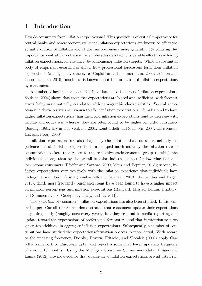
1 Introduction

How do consumers form inflation expectations? This question is of critical importance for

central banks and macroeconomists, since inflation expectations are known to affect the

actual evolution of inflation and of the macroeconomy more generally. Recognizing this

importance, central banks have in recent decades devoted considerable effort to anchoring

inflation expectations, for instance, by announcing inflation targets. While a substantial

body of empirical research has shown how professional forecasters form their inflation

expectations (among many others, see Capistran and Timmermann, 2009; Coibion and

Gorodnichenko, 2010), much less is known about the formation of inflation expectations

by consumers.

A number of factors have been identified that shape the level of inflation expectations.

Souleles (2004) shows that consumer expectations are biased and ineffi cient, with forecast

errors being systematically correlated with demographic characteristics. Several socio-

economic characteristics are known to affect inflation expectations —females tend to have

higher inflation expectations than men, and inflation expectations tend to decrease with

income and education, whereas they are often found to be higher for older consumers

(Jonung, 1981; Bryan and Venkatu, 2001; Lombardelli and Saleheen, 2003; Christensen,

Els, and Rooij, 2006).

Inflation expectations are also shaped by the inflation that consumers actually ex-

perience —first, inflation expectations are shaped much more by the inflation rate of

consumption baskets that relate to the respective socio-economic group to which the

individual belongs than by the overall inflation indices, at least for low-education and

low-income consumers (Pfajfar and Santoro, 2009; Menz and Poppitz, 2013); second, in-

flation expectations vary positively with the inflation experience that individuals have

undergone over their lifetime (Lombardelli and Saleheen, 2003; Malmendier and Nagel,

2013); third, more frequently purchased items have been found to have a higher impact

on inflation perceptions and inflation expectations (Ranyard, Missier, Bonini, Duxbury,

and Summers, 2008; Georganas, Healy, and Li, 2014).

The evolution of consumers’inflation expectations has also been studied. In his sem-

inal paper, Carroll (2003) has demonstrated that consumers update their expectations

only infrequently (roughly once every year), that they respond to media reporting and

update toward the expectations of professional forecasters, and that inattention to news

generates stickiness in aggregate inflation expectations. Subsequently, a number of con-

tributions have studied the expectations-formation process in more detail. With regard

to the updating frequency, Doepke, Dovern, Fritsche, and Slacalek (2008) apply Car-

roll’s framework to European data, and report a somewhat lower updating frequency

of around 18 months. Using the Michigan Consumer Survey microdata, Dräger and

Lamla (2012) provide evidence that quantitative inflation expectations are adjusted rel-

2

atively frequently, whereas the qualitative assessment (whether prices in general will go

up, down or stay where they are now) changes less often. Qualitatively, the expectations

tend to change mostly if the quantitative adjustment is substantial. Furthermore, they

find the updating frequency to vary over the business cycle. Coibion and Gorodnichenko

(2012) model the responsiveness of expectations to macroeconomic shocks, and confirm

the presence of imperfect information not only for consumers, but much more broadly for

professional forecasters, firms, central bankers and financial market participants.

The second aspect of Carroll (2003), the role of media reporting in inflation expec-

tations, has also been taken further by a number of subsequent studies. Inattention by

consumers has been found to be important in Mankiw and Reis (2002), Mankiw, Reis,

and Wolfers (2004) and Reis (2006). Lamla and Maag (2012) analyze the effect of media

reporting on disagreement among forecasters, and find professional forecaster disagree-

ment to be unaffected by media coverage, whereas disagreement among households in-

creases with higher and more diverse media coverage. Pfajfar and Santoro (2009) provide

evidence that the effect of news on inflation expectations differs across socio-economic

groups, and Easaw, Golinelli, and Malgarini (2013) demonstrate that the rate at which

the professional forecasts are embodied in the households’expectations depends on socio-

economic characteristics, such as education. Finally, Pfajfar and Santoro (2013) highlight

the importance of differentiating between media reporting on inflation and whether a con-

sumer has actually heard news about prices. Their study replicates Carroll’s finding that

inflation expectations get updated toward the professional forecasts using aggregate data.

However, this is not the case at the individual household level, where most consumers

who update actually revise their expectations away from the professional benchmark, but

by suffi ciently small amounts that they are dominated in the aggregate data by relatively

few households who update toward professional forecasts by large amounts. Differences

in the magnitude of revisions that take place in response to news have been identified by

Armantier, Nelson, Topa, van der Klaauw, and Zafar (2012), who find larger revisions

for agents that start off with relatively less precise expectations.

The current paper tries to better understand these findings by studying how the updat-

ing processes differ across household groups. The paper expands the previous literature

by focusing not only on the well-established socio-economic determinants of inflation ex-

pectations such as gender, education and income, but also on other characteristics such

as households with diffi cult current and expected financial situations and with pessimistic

consumer attitudes. A small number of related studies have provided some evidence in

that direction. Webley and Spears (1986) show that U.K. consumers who think they do

less well financially than during the previous year, as well as consumers who expect to

be worse off in the subsequent year, have higher inflation expectations. Similarly, del

Giovane, Fabiani, and Sabbatini (2009) and Malgarini (2009) find that inflation expec-

tations of Italian consumers are higher for respondents with pessimistic attitudes, and

3

for households in financial diffi culties. How can this be rationalized? First, if consumers

struggle to make ends meet with their available budget, this could be due to a reduction

in their income or to an increase in their expenditures —which in turn could be due

to several factors, one of them being rising prices for their consumption bundle. Under

uncertain information and information-processing constraints, it might well be that such

consumers estimate inflation to be higher than others. Second, it has been shown that

financially constrained consumers are more attentive to price changes of the goods they

purchase than more affl uent consumers (Snir and Levy, 2011). Combining this with the

well-known notion that agents are more receptive to bad than to good news (see, e.g.,

Baumeister, Bratslavsky, Finkenauer, and Vohs, 2001) might well imply that financially

constrained households arrive at a higher estimate of inflation.

To study the questions at hand, we employ the same data source that has been used

in many of the studies following Carroll (2003), namely the Michigan Consumer Survey.

This data source has a long history, allowing us to study a time sample from 1980 to 2011.

In line with current best practice, we study the microdata from this survey, which enables

us to split the respondents according to their characteristics. Our estimates are based on

nearly 70,000 observations of inflation expectations by households that are interviewed

twice, allowing us to observe how their inflation expectations change over time.

Our first key finding in this paper is that consumer attitudes as well as households’

current and expected financial situations have a bearing on inflation expectations. Con-

sumers with pessimistic attitudes about major purchases (such as purchases of durables,

houses or vehicles), who find themselves in diffi cult financial situations, or who expect

income to go down in the future have larger forecast errors, are further away from pro-

fessional forecasts and have a stronger upward bias in their expectations. Broadly, the

same holds for low-income households, lower education levels, the elderly and female

respondents, as established in the previous literature.1

We also confirm the earlier findings that consumers are responsive to news. We employ

two news measures, the first based on the survey itself (where respondents can report

whether they have recently heard news about prices), and the second following Carroll

(2003) based on intensity of news coverage related to inflation in the New York Times

and the Washington Post. While both of these measures have been used previously, e.g.

in Pfajfar and Santoro (2013), how they differ, and how each of them would have to be

interpreted, have not been discussed. In this paper, we clarify that whether respondents

have heard news about prices is very tightly linked to gasoline price inflation in the United

States. This relationship is in line with earlier evidence that frequently purchased items

(such as gasoline) shape the inflation perceptions of consumers, and also likely reflects

the fact that gasoline prices are extremely salient due to their prominent postings at gas

1See e.g. Jonung (1981), Bryan and Venkatu (2001), Lombardelli and Saleheen (2003) and Chris-tensen, Els, and Rooij (2006).

4

stations.

Interestingly, our two news measures have very different implications for consumer

inflation expectations. Having heard news about prices (reflecting predominantly large

increases in gasoline prices) increases the bias and worsens forecast accuracy. In contrast,

more intense media coverage tends to reduce the bias and improve forecast accuracy. In

that regard, our second key finding in this paper is that households with more strongly

upward-biased expectations are more responsive to media coverage, and see their bias

shrinking by more than the other household groups.

These findings have interesting implications for policy-makers and the media, sug-

gesting that more reporting about inflation improves consumers’inflation expectations,

and particularly so for consumers who are in the right tail of the distribution, i.e. have

a particularly strong upward bias.

The remainder of the paper is structured as follows. In Section 2, we describe the

data used in our empirical analysis and provide some stylized facts. Section 3 provides

an overview of the econometric approach that we employ, while Section 4 reports the

relevant results. Section 5 concludes.

2 The Data and Some Descriptive Analysis

Our household-level data contain information on a wide range of factors that influence

consumers’expectations. As such, they allow us to explore the process of expectations

updating in greater detail. In this section we describe the key features of the data set and

report some preliminary evidence on households’and professional forecasters’ inflation

expectations, as well as on the newspaper index proposed by Carroll and a direct measure

of consumers’receptiveness toward news on prices. Moreover, we report some descriptive

statistics about household-level characteristics that are accounted for as determinants of

the process of expectations formation.

2.1 Inflation Expectations

The Survey of Consumer Attitudes and Behavior is a representative survey conducted by

the Survey Research Center at the University of Michigan (Curtin, 2013). The Michigan

Survey (henceforth, MS) has been available on a monthly basis since January 1978. The

short rotating panel design constitutes its main peculiarity: 40% of prior respondents are

reinterviewed in every round, the remaining 60% being initial interviews from a random

subsample of the mainland U.S. population that has a landline telephone. Since we

are interested in how consumers update their inflation expectations, we will restrict our

analysis to the second interview, which leaves us with 67,116 observations. From a total

of 71,629 reinterviews, we lose 6.3% of observations due to question attrition (i.e., 4,513

5

individuals decided not to provide a year-ahead inflation expectation), which we will

control for in our econometric estimates.

Participants are asked two questions about expected changes in prices: first, whether

they expect prices to go up, down or stay the same in the next 12 months; second, to

provide a quantitative statement about the expected change.2

As to professional forecasts, Carroll employs the mean inflation expectation from the

Survey of Professional Forecasters (henceforth, SPF). The SPF, currently conducted by

the Federal Reserve Bank of Philadelphia, has collected and summarized forecasts from

leading private forecasting firms since 1968. The survey questionnaire is distributed once

a quarter and asks participants for quarter-by-quarter forecasts, spanning the current

and next five quarters.3

Insert Figure 1 here

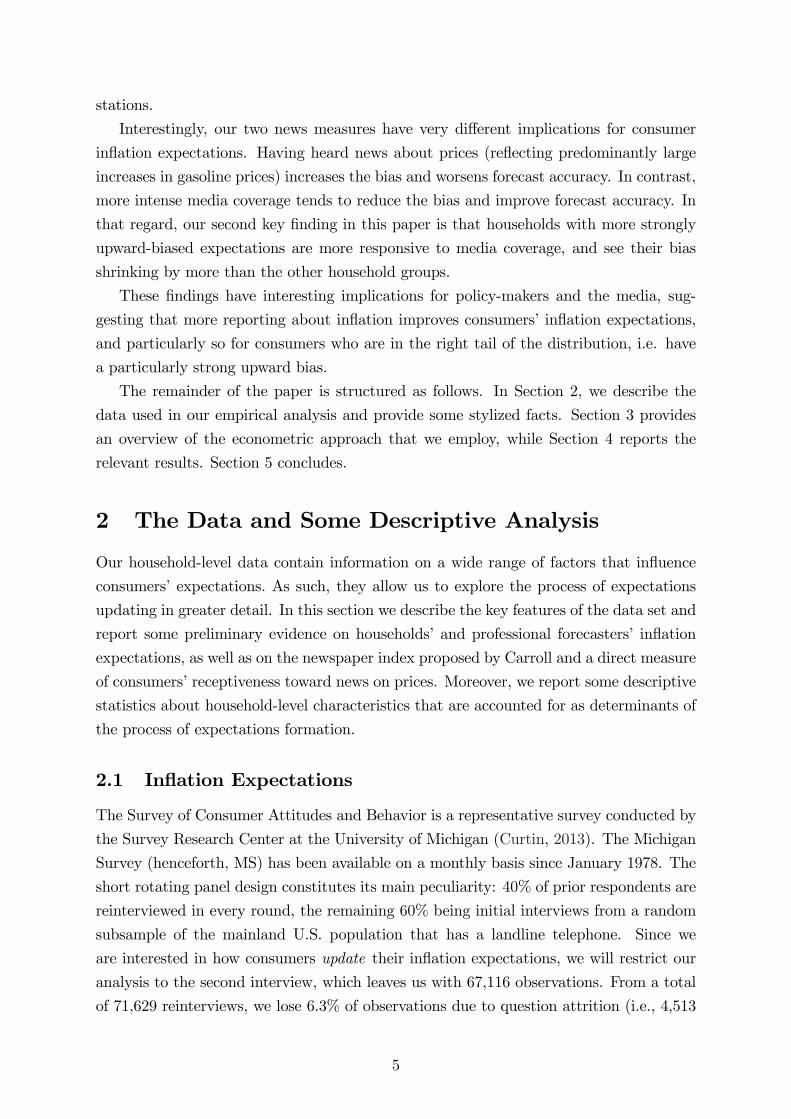
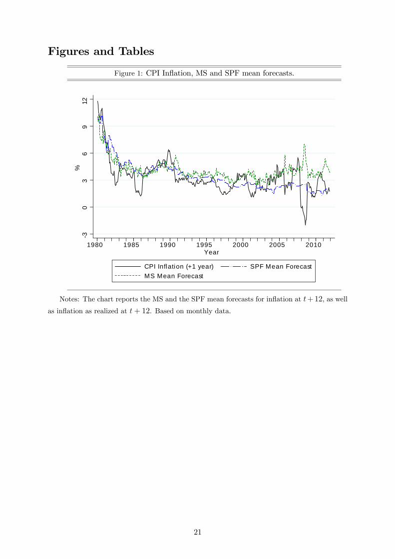
The analysis will focus on the 1980M1-2011M12 period.4 Figure 1 reports mean

forecasts of households and professionals against CPI inflation.5 Both the MS and the

SPF appear to predict inflation reasonably well, although they often fail to match periods

of low inflation. For instance, at the very end of the sample, from 2009-11, they are

considerably higher than actual inflation turned out to be. This episode has been studied

by Coibion and Gorodnichenko (2013), who suggest that, due to high oil price inflation,

household inflation expectations were elevated, which in turn help explain the "missing

disinflation" in the United States (i.e., the fact that standard Phillips curves would have

predicted a disinflation over that period that did not materialize).

2If a respondent expects prices to stay the same, the interviewer must make sure that the respondentdoes not actually expect that prices will change at the same rate at which they have changed over thepast 12 months. In line with common practice, we discard observations if the respondent expects inflationto be less than -5% or more than +30%. This rule only affects 0.7% of the observations in the sampleunder scrutiny. Curtin (1996) also adopts alternative truncation intervals, such as [-10%,50%], showingthat the key statistical properties of the resulting sample are close to invariant across different cut-offrules.

3The SPF was previously carried out as a joint product of the National Bureau of Economic Researchand the American Statistical Association on a wide variety of economic variables, including GDP growth,various measures of inflation and the rate of unemployment. For a comprehensive analysis of the SPFforecasts, the interested reader should refer to Croushore (1998). In order to obtain a monthly estimateof the SPF we may consider two options: either forecasters keep their forecast until the next surveyround, or their "monthly" forecast includes a partial adjustment to the next quarter forecast. We tookboth approaches and obtained nearly identical results. In the current version we linearly interpolatebetween quarters to account for missing monthly observations.

4SPF forecasts of CPI inflation are only available from 1981Q3. Therefore, from 1980Q1 to 1981Q3we proxy the SPF mean forecast of CPI inflation with the mean forecast of the GDP deflator. The twoseries are highly correlated.

5Inflation expectations sampled at time t are graphed with inflation 12 months later, to be in linewith the forecast target.

6

2.2 News on Inflation

A direct implication of Carroll’s view is that more media reporting should imply that

people are better informed and produce better forecasts. To test this hypothesis, we

require reliable indicators of the flow of news on inflation that the public is confronted

with. Carroll computes a yearly index of the intensity of news coverage in the New York

Times and theWashington Post. In this paper, we use the monthly version of this index

that has been constructed in Pfajfar and Santoro (2013). It is based on a search of each

of the two newspapers for inflation-related articles, converted into an index by dividing

the number of inflation-related articles by the total number of articles.6

In addition, our analysis will rely on a measure of consumers’ perceptions of new

information about prices. This is intended to complement the newspapers index proposed

by Carroll. In fact, the accuracy of a proxy based on the intensity of news coverage in

national newspapers can be questioned on different grounds. For instance, Blinder and

Krueger (2004) suggest that consumers primarily rely on information about inflation from

television, followed by local and national newspapers.7 It is also plausible to expect that

the volume of news about inflation does not necessarily match the flow of information

that is assimilated by the public. In this respect, a non-trivial discrepancy could result

from the interplay of two mutually reinforcing effects: (i) news from the media does

not necessarily reach the public uniformly and (ii) the connection between news and

inflation expectations is likely to be affected by consumers’receptiveness to the news and

the capacity to process new information. Indeed, Sims (2003) emphasizes the presence

of information-processing constraints that could be compatible with such ineffi ciencies.

Finally, it is well known that consumer inflation perceptions are shaped —in line with

the availability heuristic (Tversky and Kahneman, 1974) —by frequently purchased items

(Ranyard, Missier, Bonini, Duxbury, and Summers, 2008), such that in periods where

inflation of such items is high, consumers might be more aware and concerned about

inflation, whereas media reporting (which most likely is generally concerned with overall

inflation) need not be more intense.

In light of these considerations, it is advisable to complement the analysis with a

variable that accounts for consumers’actual perceptions of inflation. Such a variable is

directly available from the MS, where respondents are asked whether they have heard

of any changes in business conditions during the previous few months. In case of an

affi rmative response, they have the possibility to give two types of news that they have

6A potential problem connected with this type of search is that the resulting index may includearticles that do not primarily cover U.S. inflation. Accordingly, Pfajfar and Santoro (2013) tested therobustness of this methodology by restricting the search to articles that just cover U.S. inflation, andfound the results to be robust.

7Since Blinder and Krueger (2004), the Internet has become a more important source of news onvarious economic statistics.

7

heard about, among them being either higher or lower prices.8

Insert Figures 2 and 3 here

Figure 2 reports the fraction of MS respondents who have heard news about prices,

together with the newspapers index and CPI inflation. The two series display poor

correlation, suggesting that they contain two distinct measures of news. The fraction

of MS respondents who have heard news about prices exhibit more volatility than the

newspapers index. Especially in the last part of the sample it displays sizable fluctuations

that neither actual inflation nor the newspapers index presents. Splitting the series into

the share of respondents who have heard news about decreasing and increasing prices,

respectively, it is evident that most of the volatility in the overall series arises due to

movements in the share of consumers who have heard about rising prices (see Figure 3).

So what is behind this measure of news? As shown in Figure 4, the correlation be-

tween the share of respondents reporting that they have heard about price increases and

inflation of retail gasoline prices is very high (0.63).9 Based on this evidence, we inter-

pret the survey-based news measure as capturing inflation perceptions originating from

frequently-purchased items such as gasoline prices. In contrast, the correlation between

negative inflation rates in gasoline prices and the share of respondents reporting that they

have heard about decreases is much smaller (0.23), which is in line with the prospect the-

ory pioneered by Kahneman and Tversky (1979), since agents tend to manifest higher

receptiveness toward "bad" news on prices, as compared with "good" news.

Insert Figure 4 here

2.3 Household-level Attributes

The core of our econometric analysis focuses on the connection between consumers’infla-

tion expectations and a number of household-level attributes. These can be grouped in

the following categories: the current and expected financial situation, consumer attitudes

toward major purchases, and the classifications used in the previous literature, namely

gender, income, age and education of the respondent. The attributes are constructed

using the survey responses as follows:

8The MS respondents primarily report about news on unemployment, followed by news on the gov-ernment (elections) and then prices. It is important to stress that 41% of the respondents report havingheard no news at all and that in 28% of the cases only one type of news is reported. This is to say that,on average, only 31% of the respondents are confronted with a potentially binding limit of two options.Therefore, though some underreporting may affect our measure of perceived news about prices, this isnot likely to be primarily induced by the specific design of the questionnaire.

9For Figure 4, we set any negative gasoline inflation numbers to zero, to reflect the fact that thesurvey news measure only reflects having heard about price increases.

8

Financial situation

• Financial situation worse: Individuals responding "worse" to the following ques-tion: Would you say that you are better off or worse off financially than you were a

year ago? From this category, we exclude all individuals who name high(er) prices

as one reason for being worse off, in order to avoid a possible endogeneity bias.

• Financial expectations worse: Individuals responding "will be worse off" to thefollowing question: Now looking ahead - do you think that a year from now you

will be better off financially, or worse off, or just about the same as now?

• Real income expectations worse: Individuals responding "income up less than prices"to the following question: During the next year or two, do you expect that your

income will go up more than prices will go up, about the same, or less than prices

will go up?

• Nominal income expectations worse: Individuals responding "lower" to the follow-ing question: During the next 12 months, do you expect your income to be higher

or lower than during the past year?

Purchasing attitudes

• Time for durable purchases bad : Individuals responding "bad" to the followingquestion: Generally speaking, do you think now is a good or a bad time for people

to buy major household items? Again, to avoid possible endogeneity, we exclude

all respondents who respond "Prices are too high, prices going up" to the following

question: Why do you say so? (Are there any other reasons?)

• Time for house purchases bad : Individuals responding "bad" to the following ques-tion: Generally speaking, do you think now is a good time or a bad time to buy a

house? Once more, we exclude those who are pessimistic due to high(er) prices.

• Time for vehicle purchases bad : Individuals responding "bad" to the followingquestion: Speaking now of the automobile market — do you think the next 12

months or so will be a good time or a bad time to buy a vehicle, such as a car,

pickup, van, or sport utility vehicle? Also here, we exclude individuals who give

high or rising prices as a reason for their answer.

Other characteristics, following the previous literature

• Income bottom 20% : Individuals in the bottom 20% of the income distribution (as

identified by the MS).

9

• Low education: Individuals with education less than 9th grade (i.e., no high schooldiploma).

• Elderly: Respondents who are at least 65 years old.

• Female: Female respondents.

For each of these categories, we construct a dummy variable that is equal to one in

case the attribute applies, and equals zero otherwise.

Insert Figure 5 here

Figure 5 gives an impression of the time variation in household characteristics, for

the example of purchasing attitudes. It reports the share of pessimistic households, and

demonstrates that this share varies substantially over time.10 It is apparent that at the

end of the sample, with the U.S. economy going through the financial crisis and a major

recession, many more consumers felt that times were not good for major purchases.

Table 1 provides a number of summary statistics for each consumer group. It indi-

cates how many respondents fall into each category and also provides tests for whether

the news reception and the inflation expectations of the various respondent groups are

statistically significantly different from those of their peers. The table reports eight dif-

ferent statistics. First, the percentage of households who have heard news about prices

(NEWSP ). Second, the updating frequencies of respondents (UPDT ), i.e. whether their

inflation expectations change from the first to the second interview. Along with this, we

also compute the frequency of those who update toward the SPF mean forecast (UPDT F )

and those who move closer to actual inflation (UPDT π). Further, we report the average

difference between the MS household-specific forecast and the SPF mean inflation fore-

cast (BIASF ) and the average difference between the MS household-specific forecast and

CPI inflation (at the forecast horizon, BIASπ). Finally, GAPSQF is the average squared

difference between the MS household-specific forecast and the SPF mean inflation fore-

cast, and GAPSQπ is the average squared difference between the MS household-specific

forecast and CPI inflation (at the forecast horizon), providing us with a measure of their

forecast errors.

A number of interesting results emerge. The chosen household groups have higher

inflation expectations, higher updating frequencies, worse forecast errors, and tend to be

further away from the expectations of professionals than their comparator group. How-

ever, there is not much variation in the average frequency at which households update

their inflation expectations between the first and the second interview, neither toward

10Due to the lack of information about the identification of survey respondents taking part in thesecond interview, it has not been possible to retrieve reliable statistics in the following periods: 1980M3,1980M12, 1982M11, 1989M11. Therefore, we have opted to treat the corresponding datapoints as missingobservations.

10

the professional forecasters’mean forecast nor actual inflation. While these descriptive

statistics are unconditional, i.e. do not correct for possible differences in other character-

istics of the various household groups, we will see in the subsequent econometric analysis

that even controlling for other characteristics, this overall picture is confirmed.

A question that arises is to what extent the various household categories that we

distinguish are correlated, or in other words whether one can assume that they are rea-

sonably independent to warrant a separate analysis. Table 2 reports pairwise Pearson

correlations among the attributes we include in the analysis, and shows that even if all

the correlations are highly statistically significant, they are not very large from an eco-

nomic point of view; we therefore proceed on the assumption that the characteristics are

suffi ciently unrelated to warrant separate analysis and to allow a direct interpretation of

their effects.

Insert Tables 1 and 2 here

3 Econometric Frameworks

This section explains the main econometric frameworks employed in the analysis. As

mentioned earlier, out of an overall sample of 71,629 reinterviewed individuals, 4,513

individuals did not provide their inflation expectations. This may represent a potential

source of bias. In order to account for question attrition, we implement the Heckman cor-

rection (Heckman, 1979), a procedure that offers a means of correcting for non-randomly

selected samples.

3.1 Bias

The first question that we will address is whether the inflation expectations of our house-

hold groups are more upward biased than those of their peers. For that purpose, we

specify the following linear regression model:

BIASi = α1 + ciα2 +NEWSPi α3 +NEWSNα4 + xiα5 (1)

+ciNEWSPi α6 + ciNEWSNα7 + ui,

BIASi ={BIASFi , BIAS

πi

}, (2)

where BIASFi is the difference between the MS household-specific forecast and the SPF

mean inflation forecast, and BIASπi is the difference between the MS household-specific

forecast and CPI inflation (at the forecast horizon). A comparison with actual, realized

inflation will tell us about the overall bias of inflation expectations, whereas the compar-

ison with the SPF is meant to compare consumer expectations against a forecast that is

11

in principle conditional on the same information set, namely the information available at

the time of the forecast.

α1 is a constant, ci denotes the household classification of interest, NEWSPi is an

individual-specific indicator of news perception (which equals one if the interviewee has, in

the previous months, heard of recent changes in prices and zero otherwise), and NEWSN

indexes the intensity of news coverage at the time of the survey.11 xi is a vector of socio-

economic characteristics (namely gender, age, income, education, race, marital status,

location in the United States)12 and ui is assumed to be normally distributed. We also

interact the household classification variable with each of the news intensity measures.

While α2 will reveal whether the various household groups differ in their bias, the para-

meters α6 and α7 will reveal whether they differ in their response to news.

For these regressions we calculate robust standard errors using the sandwich estimator.

3.2 Expectations Updating

We will study two aspects related to the updating of inflation expectations. First, we wish

to learn whether our household groups update more often than their peers, given that

they are likely to be affected more by changes in inflation. To explore the determinants

of expectations updating at the household level, we specify a probit model. The following

variable is defined:

zi =

{1 if z∗i > 0

0 if z∗i ≤ 0, i = 1, 2, ..., N, (3)

where z∗i is the latent variable that accounts for consumers’expectations updating. Its

discrete counterpart, zi, takes the value one if the ith respondent has changed expectations

from the first interview, and zero otherwise. Since individuals are interviewed only twice,

the only reference term to determine whether expectations updating has taken place is

represented by the response in the second interview. The following latent process is

assumed:

z∗i = α1 + ciα2 +NEWSPi α3 +NEWSNα4 + xiα5 (4)

+ciNEWSPi α6 + ciNEWSNα7 + ui.

11In a robustness test, we will also include the last observed CPI inflation rate. We have furthermoreconsidered the possibility that consumers look at alternative inflation measures, such as the average rateof inflation over the six months reinterview period, but did not obtain different results.12Household income is grouped into quintiles and age is measured in integers, while education is split

into six groups: “Grade 0-8, no high school diploma,”“Grade 9-12, no high school diploma,”“Grade0-12, with high school diploma,”“4 yrs. of college, no degree,”“3 yrs. of college, with degree”and “4yrs. of college, with degree.”Race is grouped into “White except Hispanic,” “African-American exceptHispanic,” “Hispanic,” “American Indian or Alaskan Native” and “Asian or Pacific Islander,” whilemarital status is given as “Married/with a partner,” “Divorced,” “Widowed,” “Never married.”Finally,the region of residence is grouped into “West,” “North Central,” “Northeast,” “South.”

12

Standard errors for the marginal effects are calculated with the delta method (Oehlert,

1992).

A second question related to the updating of expectations is whether consumers up-

date toward the SPF or actual inflation, i.e. whether the updated expectations have

improved over time. To check for updating toward the SPF, we define a dummy variable

that is equal to one if abs(Ei,t2πt2+12 − EFt2πt2+12) < abs(Ei,t1πt1+12 − EF

t1πt1+12), where

EFt is the mean expectation operator of the SPF at time t, t1 denotes the time of the first

interview, and t2 the time of the second interview. For updating toward actual inflation,

the equivalent dummy variable is defined to be equal to one if abs(Ei,t2πt2+12− πt2+12) <abs(Ei,t1πt1+12 − πt1+12). Again, this variable is modelled in a probit framework.

4 The Determinants of Consumer Inflation Expecta-

tions

Having specified the data and the econometric model, we next discuss the econometric

results. First, we analyze whether consumer inflation expectations are biased relative to

professional forecasts and relative to actual inflation. Then, we study the updating of

expectations.

4.1 Bias

Turning to the analysis of the bias, Tables 3 and 4 confirm the previous findings that

consumer inflation expectations are biased upwards. The constant reflects the conditional

bias of a representative agent with the following characteristics: white (non-Hispanic),

married, male, 40 years old, high school diploma, an income in the middle quintile of the

distribution and living in the North-Center of the country; the bias is estimated to be

statistically significant and positive both when we compare inflation expectations against

those of professional forecasters in Table 3 and when we compare against realized inflation

in Table 4.

While the inflation expectations of the representative consumer are biased upwards,

the bias is substantially larger for the household groups that we study. With the exception

of respondents who find their current financial situation to have worsened, all other groups

have a larger bias. Relative to professional forecasts, the magnitude ranges from 0.36%

for respondents who are pessimistic about the purchases of durables to 1.2% for those

who expect real income to decline. Similar orders of magnitude are also observed for the

bias of the various socio-economic groups that the literature had pointed out previously

(e.g., 0.5% for females, and 1.3% for the elderly). These results also hold when consumer

inflation expectations are compared to actual inflation in Table 4.

13

Having heard news about prices, which is heavily influenced by increases in gaso-

line prices, increases the bias by around 1%. Interestingly, this effect does not differ

across household groups, suggesting that the effect of gasoline price inflation on inflation

expectations is universal, and relatively homogeneous across different consumer types.

Contrary to having heard news about prices, more media reporting about inflation tends

to reduce the bias in inflation expectations. A one-standard-deviation increase in media

reporting (i.e., a change in the index by 4%), ceteris paribus, leads to a reduction in the

bias of around 0.3 to 0.4% when measured against actual inflation, and of around 0.7

to 0.8% when measured against the SPF. The effect is estimated to be different across

household groups, with a larger reduction in the bias of pessimistic consumers and those

in dire financial situations; when calculated relative to actual inflation, the effect often is

twice as large as for the average consumer. This result suggests that more news coverage

is beneficial in that (i) it reduces the bias in inflation expectations of the average con-

sumer, and (ii) it does so particularly for those consumer groups that had a larger bias

to start with. Finally, the inference confirms that it is important to account for question

attrition, as we can appreciate from the statistical significance of the coeffi cient attached

to the residuals from the selection regression (rho). This property tends to hold for most

of the subsequent econometric analysis.

Insert Tables 3 and 4 here

4.2 Expectations Updating

Table 5 reports results for the determinants of the updating frequency, by providing

marginal partial effects. A number of results stand out. First, it is apparent that the

financial situation and the purchasing attitudes have a bearing on how often households

update their inflation expectations — those with diffi cult current or expected financial

situations and those who believe that times are bad for purchasing durables, houses or

vehicles are 2 to 4% more likely to change their inflation expectations between the two

survey interviews, an effect that is estimated to be highly statistically significant in all

cases. Similar results are also obtained for the standard categorization variables age and

gender —only education does not seem to matter.

Consumers who have recently received news about prices are also more likely to up-

date their inflation expectations, and the same holds true for a higher news intensity

in the media. Finally, even if there are different updating frequencies across the house-

hold groups, there is no evidence that the updating depends on the news intensity in a

differential manner.

Insert Table 5 here

14

Finally, we look at the prediction of Carroll’s (2003) model, namely that more media

reporting will lead consumers to update toward a more rational forecast. Table 6 shows

results for the probit model that tests whether consumers’inflation expectations in the

second interview are closer to those of the SPF than in the first interview; Table 7

compares whether inflation expectations move closer to actual inflation outcomes in the

second interview.

Looking at Table 6, it is not apparent whether consumers do indeed update their

forecast toward the SPF. For some model specifications, it seems that consumers, on

average, update away from professional forecasts when media reporting intensifies, while

for most model specifications, no statistically significant effect is found. This is in line

with the previous evidence by Pfajfar and Santoro (2013), who found that some consumers

update away from professional forecasts, whereas others update toward them —in which

case we would not expect to find statistically significant effects. Their paper furthermore

shows that most consumers update away from professional forecasts, which is consistent

with us finding such an effect in some specifications.

When we study whether consumers’expectations are updated toward actual inflation,

i.e. whether actual forecast errors become smaller, results are more interesting (see Table

7). In line with the results in the previous section, we find that consumers who have

heard news about rising prices will find their forecast deteriorating, whereas more news

reporting in the media tends to make consumers update their forecasts toward actual

inflation —even if the magnitude of the effect is small. Interestingly, these effects are not

significantly different for the various consumer groups that we distinguish. In combination

with the finding that their bias is reduced more strongly in response to media reporting,

this suggests that the average consumer adjusts toward actual inflation, but that our

consumer groups adjust by larger amounts.

Insert Tables 6 and 7 here

4.3 Robustness

We have conducted several robustness checks to investigate the sensitivity of our results

to our modelling choices. For brevity, we will only show those that relate to the bias of

consumers relative to actual inflation (i.e., those reported in Table 4), but results generally

hold also for the other analyses. For the first robustness check, we added lagged actual

inflation as an explanatory variable to the regression (see Table 8). As a matter of fact,

consumers are responsive to past developments of inflation, with higher inflation rates

lowering the bias. The magnitudes by which the bias of our consumer groups is elevated

relative to the others remains largely unchanged, as does the effect of perceived news.

The coeffi cients on media reporting are somewhat smaller (reflecting the fact that media

reporting is more intense when inflation is high), but the sign remains unchanged: more

15

media reporting lowers the bias, and much more so for our respective consumer groups

(with the magnitude of the interaction terms being roughly unchanged).13

Another robustness test checks for those consumers who are pessimistic about major

purchases, or see themselves in a diffi cult financial situation, but who mention that this

is due to increasing prices (whereas, so far, these had been excluded from the household

groups). Of course, we would expect these consumers to have a substantially larger

bias, and this is indeed the case, as shown in Table 9. The exception is consumers who

think that times are bad to purchase a house due to prices —which is intuitive, since

these respondents most likely have house prices in mind when answering that question,

so they need not have a larger bias with regard to consumer prices. All other results go

through with this robustness test —perceived news increases the bias, and media reporting

decreases it, and particularly so for the pessimistic households.

Insert Tables 8 to 10 here

A third robustness test relates to those consumers who have changed their attitudes

between interviews (i.e., those who changed their attribute over time, and fell into the

category during their second interview, but not during the first interview). Results for

the level of the bias, shown in Table 10, are qualitatively unchanged — those who fall

into the respective category only during the second interview have a significantly larger

upward bias. However, their reaction to media reporting is now estimated to be the same

as for all the other consumers, suggesting that media reporting primarily helps reduce

the elevated bias of persistently pessimistic consumers.

Finally, our benchmark model contains a variable that indicates whether a respondent

has heard news about prices. One might wonder whether the effect would be more

prominent had we only included respondents who have heard news about rising prices.

As discussed earlier, most of the observations for this variable originate from respondents

who have heard about rising prices, whereas very few report to have heard about declining

prices. Replacing our variable for perceived news to include only news about rising prices

does not alter our results (which are not shown, for brevity).

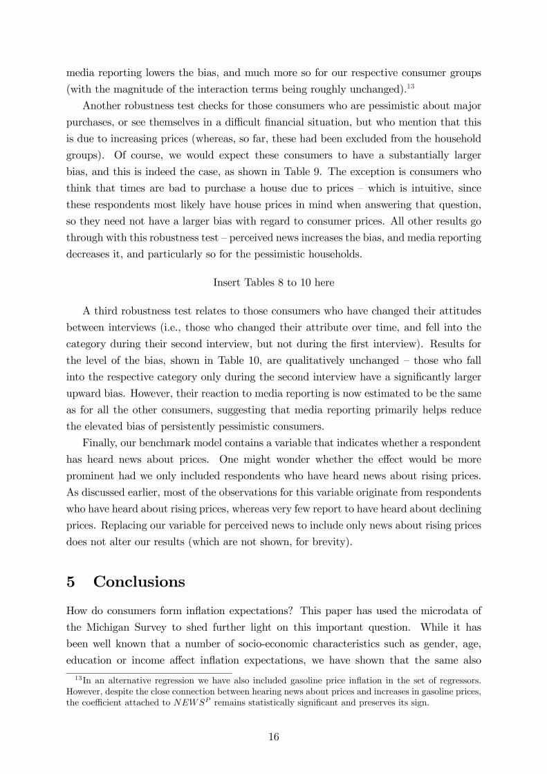
5 Conclusions

How do consumers form inflation expectations? This paper has used the microdata of

the Michigan Survey to shed further light on this important question. While it has

been well known that a number of socio-economic characteristics such as gender, age,

education or income affect inflation expectations, we have shown that the same also

13In an alternative regression we have also included gasoline price inflation in the set of regressors.However, despite the close connection between hearing news about prices and increases in gasoline prices,the coeffi cient attached to NEWSP remains statistically significant and preserves its sign.

16

holds true for consumer attitudes. Having pessimistic attitudes toward the purchase of

durables or homes, experiencing or expecting financial diffi culties, as well as expectations

that household income will go down in the future affects inflation expectations in a

substantial fashion. It increases the upward bias that is anyway inherent in consumer

inflation expectations and worsens forecast accuracy. The effects are not only found to

be statistically significant, they are substantial in magnitude.

Generally, consumer inflation expectations are highly sensitive to perceived news

about rising prices, which themselves are tightly connected to the evolution of gaso-

line prices. Rising gasoline prices are being noticed much more than falling gasoline

prices, and they lead consumers to revise their expectations more frequently, but worsen

their bias. This is in contrast to media reporting about inflation, which similarly tends

to induce a higher updating frequency of consumers. Importantly, however, more in-

tense media reporting lowers the bias, and especially so for pessimistic households and

households in dire financial situations.

The findings have important implications for policy-makers. They suggest that more

communication about inflation improves consumers’inflation expectations, and particu-

larly so for consumers who are in the right tail of the distribution, i.e. those who have a

particularly strong upward bias.

References

Armantier, O., S. Nelson, G. Topa, W. van der Klaauw, and B. Zafar (2012):

“The price is right: updating of inflation expectations in a randomized price informa-

tion experiment,”Staff Reports 543, Federal Reserve Bank of New York.

Baumeister, R., E. Bratslavsky, C. Finkenauer, and K. Vohs (2001): “Bad is

stronger than good,”Review of General Psychology, 5, 323—370.

Blinder, A. S., and A. B. Krueger (2004): “What Does the Public Know about

Economic Policy, and How Does It Know It?,”Brookings Papers on Economic Activity,

35(2004-1), 327—397.

Bryan, M. F., and G. Venkatu (2001): “The demographics of inflation opinion sur-

veys,”Economic Commentary, (15).

Capistran, C., and A. Timmermann (2009): “Disagreement and Biases in Inflation

Expectations,”Journal of Money, Credit and Banking, 41(2-3), 365—396.

Carroll, C. D. (2003): “Macroeconomic Expectations Of Households and Professional

Forecasters,”The Quarterly Journal of Economics, 118(1), 269—298.

17

Christensen, C., P. Els, and M. Rooij (2006): “Dutch Households’Perceptions of

Economic Growth and Inflation,”De Economist, 154(2), 277—294.

Coibion, O., and Y. Gorodnichenko (2010): “Information Rigidity and the Expec-

tations Formation Process: A Simple Framework and New Facts,” NBER Working

Papers 16537, National Bureau of Economic Research, Inc.

(2012): “What Can Survey Forecasts Tell Us about Information Rigidities?,”

Journal of Political Economy, 120(1), 116 —159.

(2013): “Is The Phillips Curve Alive and Well After All? Inflation Expecta-

tions and the Missing Disinflation,”NBER Working Papers 19598, National Bureau of

Economic Research, Inc.

Croushore, D. (1998): “Evaluating inflation forecasts,”Working Papers 98-14, Federal

Reserve Bank of Philadelphia.

Curtin, R. (1996): “Procedure to estimate price expectations,”Mimeo, University of

Michigan.

(2013): “Survey of Consumers,” Discussion Paper mimeo, Survey Reserach

Center, University of Michigan.

del Giovane, P., S. Fabiani, and R. Sabbatini (2009): “What’s Behind ‘Inflation

Perceptions’? A Survey-Based Analysis of Italian Consumers,”Giornale degli Econo-

misti, 68(1), 25—52.

Doepke, J., J. Dovern, U. Fritsche, and J. Slacalek (2008): “The Dynamics of

European Inflation Expectations,”Topics in Macroeconomics, 8(1), 1540—1540.

Dräger, L., and M. J. Lamla (2012): “Updating inflation expectations: Evidence

from micro-data,”Economics Letters, 117, 807—810.

Easaw, J., R. Golinelli, and M. Malgarini (2013): “What determines households

inflation expectations? Theory and evidence from a household survey,”European Eco-

nomic Review, 61(C), 1—13.

Georganas, S., P. J. Healy, and N. Li (2014): “Frequency bias in consumers’per-

ceptions of inflation: An experimental study,” European Economic Review, 67(C),

144—158.

Heckman, J. J. (1979): “Sample Selection Bias as a Specification Error,”Econometrica,

47(1), 153—61.

18

Jonung, L. (1981): “Perceived and Expected Rates of Inflation in Sweden,”American

Economic Review, 71(5), 961—68.

Kahneman, D., and A. Tversky (1979): “Prospect Theory: An Analysis of Decision

under Risk,”Econometrica, 47(2), 263—91.

Lamla, M. J., and T. Maag (2012): “The Role of Media for Inflation Forecast Dis-

agreement of Households and Professionals,”Journal of Money, Credit and Banking,

44(7), 1325—1350.

Lombardelli, C., and J. Saleheen (2003): “Public expectations of UK inflation,”

Bank of England Quarterly Bulletin, 43, 281—290.

Malgarini, M. (2009): “Quantitative Inflation Perceptions and Expectations of Italian

Consumers,”Giornale degli Economisti, 68(1), 53—80.

Malmendier, U., and S. Nagel (2013): “Learning from Inflation Experiences,”

Mimeo, UC Berkeley and Stanford University.

Mankiw, N. G., and R. Reis (2002): “Sticky Information Versus Sticky Prices: A

Proposal To Replace The New Keynesian Phillips Curve,”The Quarterly Journal of

Economics, 117(4), 1295—1328.

Mankiw, N. G., R. Reis, and J. Wolfers (2004): “Disagreement about Inflation

Expectations,”NBER Macroeconomics Annual 2003, 18, 209—248.

Menz, J.-O., and P. Poppitz (2013): “Households’disagreement on inflation expec-

tations and socioeconomic media exposure in Germany,”Discussion Papers 27/2013,

Deutsche Bundesbank, Research Centre.

Oehlert, G. W. (1992): “A Note on the Delta Method,”The American Statistician,

46(1), pp. 27—29.

Pfajfar, D., and E. Santoro (2009): “Asymmetries in Inflation Expectations Across

Sociodemographic Groups,”Mimeo, Tilburg University.

(2013): “News on Inflation and the Epidemiology of Inflation Expectations,”

Journal of Money, Credit and Banking, 45(6), 1045—1067.

Ranyard, R., F. D. Missier, N. Bonini, D. Duxbury, and B. Summers (2008):

“Perceptions and expectations of price changes and inflation: A review and conceptual

framework,”Journal of Economic Psychology, 29(4), 378—400.

Reis, R. (2006): “Inattentive consumers,”Journal of Monetary Economics, 53(8), 1761—

1800.

19

Sims, C. A. (2003): “Implications of rational inattention,” Journal of Monetary Eco-

nomics, 50(3), 665—690.

Snir, A., and D. Levy (2011): “Shrinking Goods and Sticky Prices: Theory and

Evidence,”Working Paper Series 17/11, The Rimini Centre for Economic Analysis.

Souleles, N. S. (2004): “Expectations, Heterogeneous Forecast Errors, and Consump-

tion: Micro Evidence from the Michigan Consumer Sentiment Surveys,” Journal of

Money, Credit and Banking, 36(1), 39—72.

Tversky, A., and D. Kahneman (1974): “Judgment under uncertainty: Heuristics

and biases,”Science, 185, 1124—1131.

Webley, P., and R. Spears (1986): “Economic preferences and inflationary expecta-

tions,”Journal of Economic Psychology, 7(3), 359—369.

20

Figures and Tables

Figure 1: CPI Inflation, MS and SPF mean forecasts.­3

03

69

12%

1980 1985 1990 1995 2000 2005 2010Year

CPI Inflation (+1 year) SPF Mean ForecastMS Mean Forecast

Notes: The chart reports the MS and the SPF mean forecasts for inflation at t+12, as well

as inflation as realized at t+ 12. Based on monthly data.

21

Figure 2: Perceived news and media reporting.

05

1015

2025

30%

1980 1985 1990 1995 2000 2005 2010Year

CPI Inflation Heard about changing pricesNews Stories

Notes: The chart reports CPI inflation as recorded for a given time period t, as well as the

share of respondents in the MS in period t answering that they have heard news about prices

("perceived news") and the index about media reporting related to inflation in period t ("news

stories"). Based on monthly data.

22

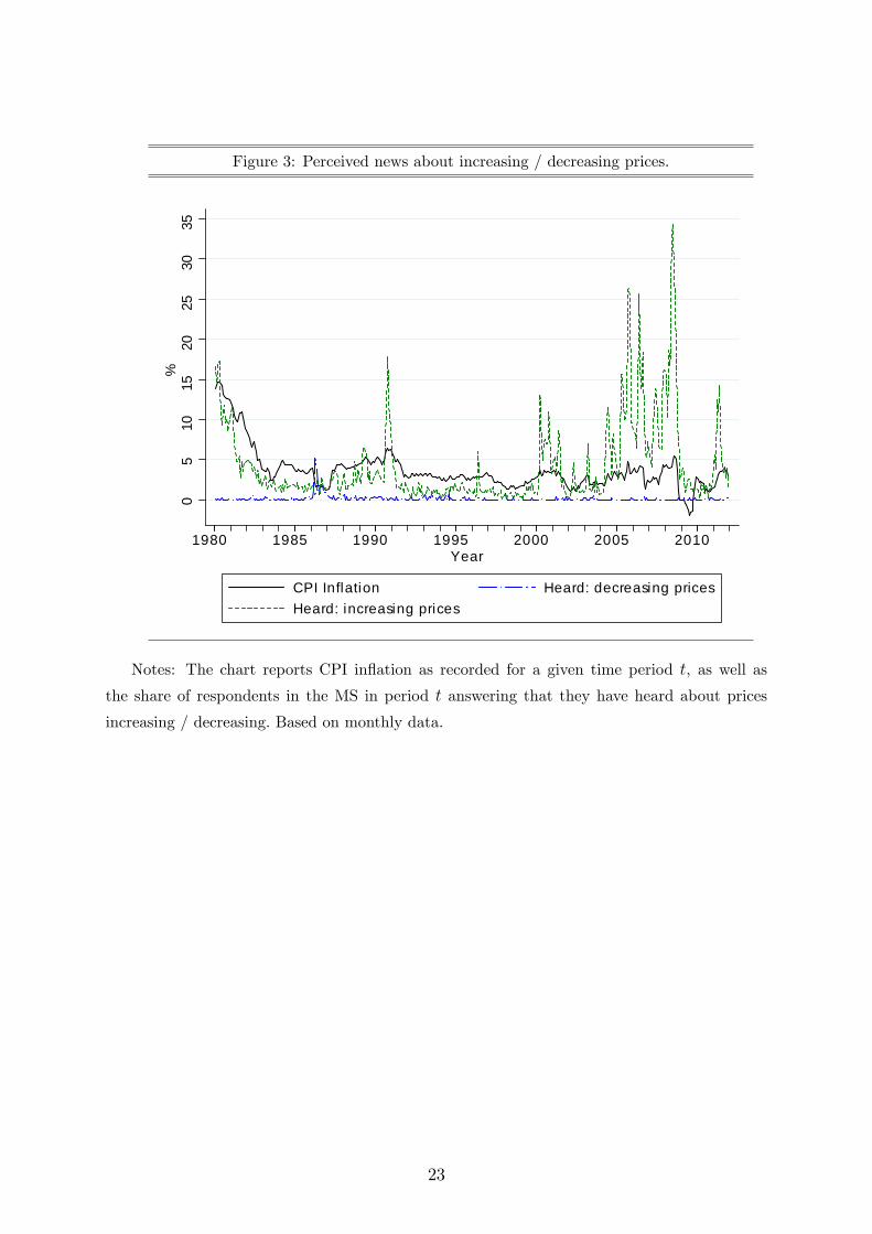
Figure 3: Perceived news about increasing / decreasing prices.

05

1015

2025

3035

%

1980 1985 1990 1995 2000 2005 2010Year

CPI Inflation Heard: decreasing pricesHeard: increasing prices

Notes: The chart reports CPI inflation as recorded for a given time period t, as well as

the share of respondents in the MS in period t answering that they have heard about prices

increasing / decreasing. Based on monthly data.

23

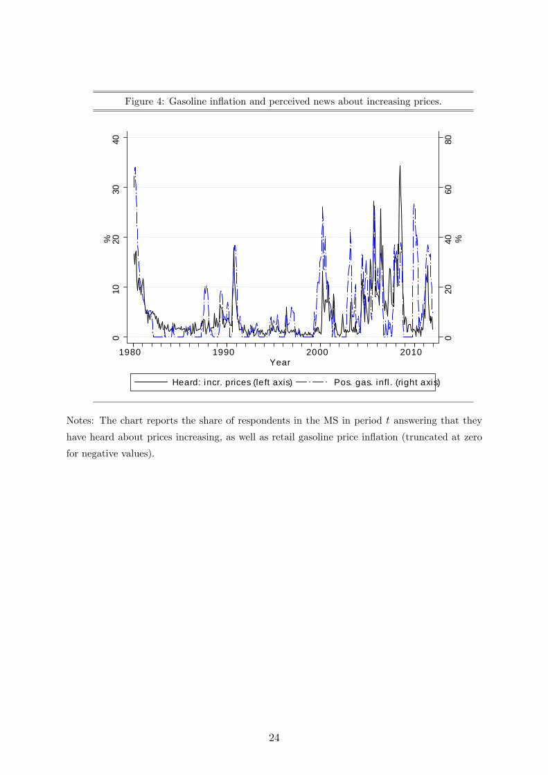
Figure 4: Gasoline inflation and perceived news about increasing prices.

020

4060

80%

010

2030

40%

1980 1990 2000 2010Year

Heard: incr. prices (left axis) Pos. gas. infl . (right axis)

Notes: The chart reports the share of respondents in the MS in period t answering that they

have heard about prices increasing, as well as retail gasoline price inflation (truncated at zero

for negative values).

24

Figure 5: Share of pessimistic households.

05

1015

2025

3035

4045

50%

1980 1985 1990 1995 2000 2005 2010Year

Durables VehiclesHouses

Notes: The chart reports the share of respondents in the MS in period t answering that the

time for purchasing durables / vehicles / houses is bad.

25

Table1:Descriptivestatistics.

OBS

NEW

SPU

PDT

UPD

TF

UPD

Tπ

BIAS

FBI

ASπ

GAPS

QF

GAPS

Qπ

Ove

rall 

sam

ple

67,1

164.

4474

.52

51.6

351

.18

0.24

0.51

16.2

217

.39

Fina

ncia

l situ

atio

n w

orse

Fina

ncia

l situ

atio

n w

orse

16,1

583.

6674

.89*

**51

.18

50.7

90.

41**

*0.

61**

*16

.14

16.9

8Fi

nanc

ial e

xpec

tatio

ns w

orse

12,4

416.

33**

*77

.32*

**51

.95

50.7

40.

80**

*1.

11**

*21

.02*

**22

.96*

**Re

al in

com

e ex

pect

atio

ns w

orse

33,1

624.

99**

*76

.77*

**51

.86

51.2

30.

70**

*0.

95**

*18

.95*

**20

.50*

**N

omin

al in

com

e ex

pect

atio

nsw

orse

13,9

834.

65*

75.6

7***

51.8

351

.75*

0.65

***

0.91

***

19.0

2***

20.2

2***

Purc

hasi

ng a

ttitu

des:

 bad

 tim

e fo

rDu

rabl

e pu

rcha

ses

15,0

794.

4776

.11*

**52

.44*

*52

.01*

*0.

55**

*0.

85**

*18

.49*

**20

.12*

**Ho

use 

purc

hase

s16

,749

5.15

***

76.6

0***

51.8

851

.45

0.34

***

0.77

***

21.3

8***

22.8

1***

Vehi

cle 

purc

hase

s14

,490

5.89

***

76.3

4***

51.3

851

.60

0.61

***

0.86

***

19.4

6***

21.1

4***

Oth

ers

Inco

me 

bott

om 2

0%10

,400

3.40

75.1

4*51

.60

50.9

60.

80**

*1.

11**

*23

.72*

**24

.82*

**Lo

w e

duca

tion

1,99

93.

0574

.44

50.1

852

.38

­0.0

90.

3725

.73*

**26

.66*

**El

derly

 (Age

 65+

)10

,486

4.02

72.6

750

.72

50.2

90.

48**

*0.

67**

*18

.27*

**19

.42*

**Fe

mal

e34

,912

4.13

74.7

051

.52

51.5

3**

0.53

***

0.81

***

19.8

3***

21.2

6***

Notes:Thetablecontainsdescriptivestatistics(columns)conditionalonvariousattributes(rows).OBS:numberofuncensoredobservations;

NEWSP:averageshareofhouseholdsobservingnews;UPDT:averagefrequencyatwhichhouseholdsupdatetheirinflation

expectations

betweenthefirstandthesecondinterview;UPDTF:averagefrequencyatwhichhouseholdsupdatetheirinflationexpectationsbetweenthefirst

andthesecondinterviewtowardtheprofessionalforecasters’meanforecast;UPDTF:averagefrequencyatwhichhouseholdsupdatetheirinflation

expectationsbetweenthefirstandthesecondinterviewtowardactualinflation;BIASF:averagedifferencebetweenconsumers’inflationforecasts

andtheSPFmeaninflationforecasts;BIASπ:averagedifferencebetweenconsumers’inflationforecastsandCPIinflation;GAPSQF:average

squareddifferencebetweenconsumers’inflationforecastsandtheSPFmeaninflationforecasts;GAPSQπ:averagesquareddifferencebetween

consumers’inflationforecastsandCPIinflation.∗∗∗ /∗∗/∗denotesstatisticalsignificanceatthe1/5/10%levelofthetestthateachentryisstrictly

lowerthanitscounterpartcomputedfrom

therestoftheoverallsamplewithtwo-samplet-tests(withequalvariances).

26

Table2:Pairwisecorrelations.

Fina

ncia

lsit

uatio

nFi

nanc

ial

expe

ctat

i­on

s

Real

expe

cted

inco

me

Nom

inal

expe

cted

inco

me

Dura

ble

purc

hase

sHo

use

purc

hase

sVe

hicl

epu

rcha

ses

Inco

me

bott

om20

%

Low

 edu

­ca

tion

Elde

rly(A

ge 6

5+)

Fem

ale

Fina

ncia

l situ

atio

n w

orse

Fina

ncia

l situ

atio

n1

Fina

ncia

l exp

ecta

tions

0.14

9***

1Re

al e

xpec

ted 

inco

me

0.29

6***

0.43

6***

1N

omin

al e

xpec

ted 

inco

me

0.29

2***

0.32

7***

0.40

4***

1Pu

rcha

sing

 att

itude

s: b

ad ti

me 

for

Dura

ble 

purc

hase

s0.

209*

**0.

194*

**0.

289*

**0.

211*

**1

Hous

e pu

rcha

ses

0.17

5***

0.22

7***

0.32

6***

0.19

1***

0.28

1***

1Ve

hicl

e pu

rcha

ses

0.18

2***

0.19

9***

0.28

6***

0.19

3***

0.34

6***

0.29

6***

1O

ther

sIn

com

e bo

ttom

 20%

0.19

6***

0.15

6***

0.26

3***

0.16

4***

0.14

2***

0.19

0***

0.15

4***

1Lo

w e

duca

tion

0.05

8***

0.11

7***

0.12

2***

0.07

6***

0.06

4***

0.10

9***

0.06

9***

0.25

4***

1El

derly

 (Age

 65+

)0.

095*

**0.

225*

**0.

287*

**0.

194*

**0.

120*

**0.

142*

**0.

132*

**0.

316*

**0.

234*

**1

Fem

ale

0.01

6***

­0.0

010.

027*

**0.

011*

**0.

014*

**0.

017*

**0.

007*

**0.

071*

**0.

004

0.03

6***

1

Fina

ncia

l situ

atio

n w

orse

Purc

hasi

ng a

tt.: 

bad 

time 

for

Oth

ers

Notes:Thetablereportspairwisecorrelationsamongthevariablesemployedintheregressionanalysis.∗∗∗denotesstatisticalsignificanceatthe

1%level.

27

Table3:Determinantsofbiasrelativetoprofessionalforecasts.

Fina

ncia

lsit

uatio

nFi

nanc

ial

expe

ctat

i­on

s

Real

expe

cted

inco

me

Nom

inal

expe

cted

inco

me

Dura

ble

purc

hase

sHo

use

purc

hase

sVe

hicl

epu

rcha

ses

Inco

me

bott

om20

%

Low

 edu

­ca

tion

Elde

rly(A

ge 6

5+)

Fem

ale

HH c

hara

cter

istic

­0.1

014

1.05

61**

*1.

1504

***

0.91

41**

*0.

3604

***

0.76

65**

*0.

6208

***

0.85

37**

*1.

1027

***

1.30

13**

*0.

5063

***

(0.1

052)

(0.1

188)

(0.0

893)

(0.1

144)

(0.1

057)

(0.1

053)

(0.1

058)

(0.1

441)

(0.3

461)

(0.1

307)

(0.0

891)

NEW

SP1.

1548

***

1.07

01**

*0.

9642

***

1.14

39**

*1.

1500

***

1.13

65**

*1.

0357

***

1.19

84**

*1.

1483

***

1.15

30**

*1.

2151

***

(0.0

982)

(0.0

949)

(0.1

136)

(0.0

981)

(0.0

963)

(0.0

975)

(0.0

992)

(0.0

893)

(0.0

867)

(0.0

924)

(0.1

036)

NEW

SP *

 Ch.

0.00

230.

1100

0.23

340.

0054

0.02

480.

0374

0.34

81*

­0.3

037

0.58

71­0

.026

5­0

.116

4(0

.206

3)(0

.213

5)(0

.168

8)(0

.207

9)(0

.216

0)(0

.203

5)(0

.199

3)(0

.307

0)(0

.770

0)(0

.258

1)(0

.173

4)N

EWSN

­0.1

904*

**­0

.185

8***

­0.1

754*

**­0

.173

7***

­0.1

837*

**­0

.172

9***

­0.1

784*

**­0

.178

2***

­0.1

829*

**­0

.165

3***

­0.1

777*

**(0

.005

7)(0

.005

6)(0

.006

8)(0

.005

6)(0

.005

8)(0

.006

2)(0

.005

8)(0

.005

4)(0

.005

2)(0

.005

5)(0

.006

6)N

EWSN

 * C

h.0.

0109

­0.0

382*

**­0

.033

8***

­0.0

668*

**­0

.015

9­0

.055

8***

­0.0

363*

**­0

.065

3***

­0.1

616*

**­0

.161

4***

­0.0

198*

*(0

.012

0)(0

.012

5)(0

.009

8)(0

.012

9)(0

.011

7)(0

.010

7)(0

.011

6)(0

.014

9)(0

.031

4)(0

.014

5)(0

.009

8)Co

nsta

nt1.

8028

***

1.75

09**

*1.

3887

***

1.62

59**

*1.

6919

***

1.59

03**

*1.

6361

***

1.68

74**

*1.

7254

***

1.50

23**

*1.

6832

***

(0.1

028)

(0.1

015)

(0.1

056)

(0.1

011)

(0.1

030)

(0.1

040)

(0.1

025)

(0.1

007)

(0.1

001)

(0.1

084)

(0.1

061)

Test

 10.

000

0.00

00.

000

0.00

00.

000

0.00

00.

000

0.00

20.

023

0.00

00.

000

Test

 20.

000

0.00

00.

000

0.00

00.

000

0.00

00.

000

0.00

00.

000

0.00

00.

000

Rho

0.97

0***

0.96

9***

0.97

0***

0.97

1***

0.97

0***

0.97

0***

0.97

0***

0.97

0***

0.97

0***

0.97

0***

0.97

0***

N71

629

7162

971

629

7162

971

629

7162

971

629

7162

971

629

7162

971

629

Chi2

2077

.440

2358

.158

2809

.340

2157

.330

2120

.170

2128

.656

2151

.058

2099

.252

2087

.745

2195

.251

2108

.318

Fina

ncia

l situ

atio

n w

orse

Purc

hasi

ng a

ttitu

des:

 bad

 tim

e fo

rO

ther

s

Notes:Thetablereportsresultsbasedonequation(1),explainingthedifferencebetweenconsumerexpectationsandtheSurveyofProfessional

Forecasters.Allmodelscontrolforgender,age,income,education,race,maritalstatus,locationintheUnitedStates.Therelevanthousehold

characteristicisreportedinthecolumnheader.ThedefinitionsofthesecharacteristicsaredescribedinSection2.3.NEWSPisanindividual-specific

indicatorofnewsperception(whichequalsoneiftheintervieweehasheardofrecentchangesinpricesandzerootherwise),NEWSNindexesthe

intensityofinflation-relatednewscoverageinthemedia.Test1denotesp-valuesofaChi2(1)testofNEWSP+NEWSP∗characteristic=0.

Test2denotesp-valuesofaChi2(1)testofNEWSN+NEWSN∗characteristic=0.Ndenotesthenumberofobservations.Rhodenotes

thecoefficienton

theresidualsoftheselectionequation

inthemainregression

(whichalsoincludesinthesetofregressorssomeinteraction

termsbetweendifferenthouseholds’socio-demographiccharacteristics).Numbersinparenthesesarestandarderrors.***/**/*denotesstatistical

significanceatthe1%/5%/10%

level.

28

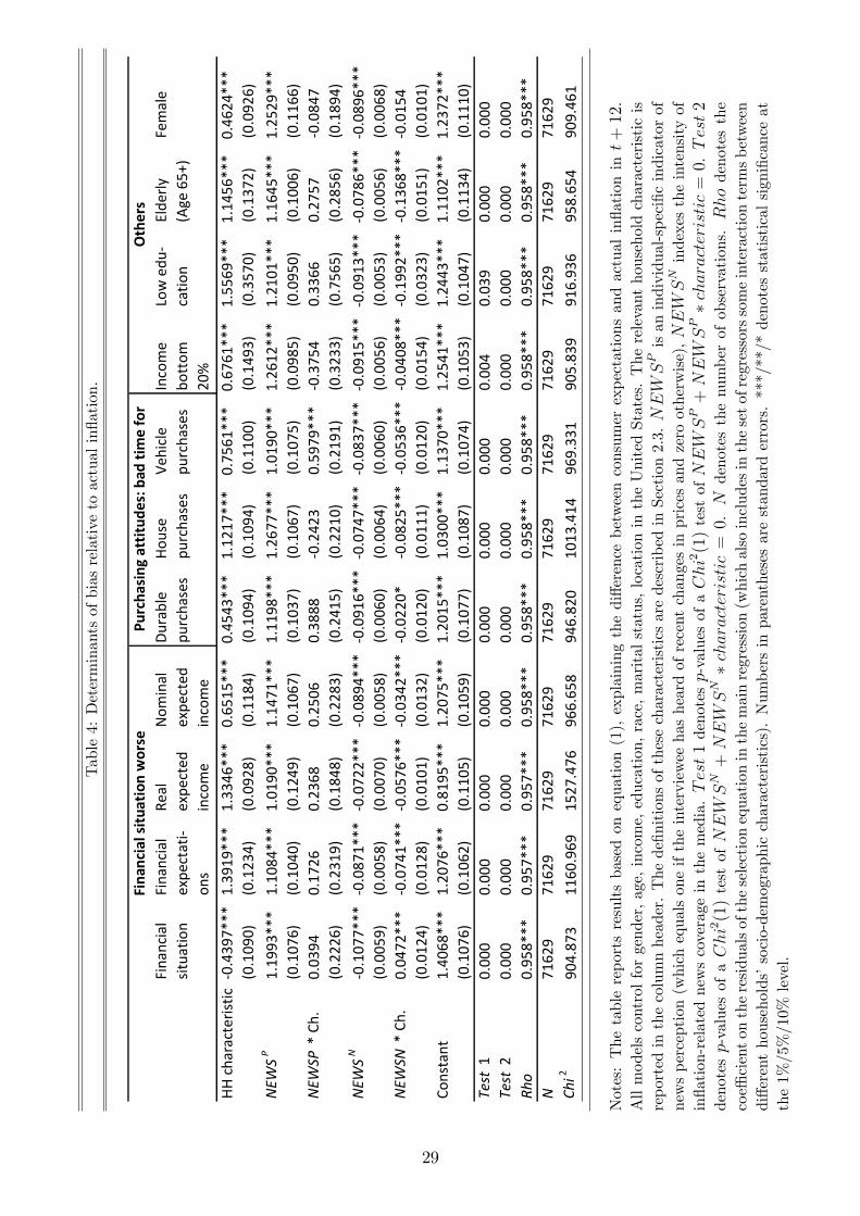
Table4:Determinantsofbiasrelativetoactualinflation.

Fina

ncia

lsit

uatio

nFi

nanc

ial

expe

ctat

i­on

s

Real

expe

cted

inco

me

Nom

inal

expe

cted

inco

me

Dura

ble

purc

hase

sHo

use

purc

hase

sVe

hicl

epu

rcha

ses

Inco

me

bott

om20

%

Low

 edu

­ca

tion

Elde

rly(A

ge 6

5+)

Fem

ale

HH ch

arac

teris

tic­0

.439

7***

1.39

19**

*1.

3346

***

0.65

15**

*0.

4543

***

1.12

17**

*0.

7561

***

0.67

61**

*1.

5569

***

1.14

56**

*0.

4624

***

(0.1

090)

(0.1

234)

(0.0

928)

(0.1

184)

(0.1

094)

(0.1

094)

(0.1

100)

(0.1

493)

(0.3

570)

(0.1

372)

(0.0

926)

NEW

SP1.

1993

***

1.10

84**

*1.

0190

***

1.14

71**

*1.

1198

***

1.26

77**

*1.

0190

***

1.26

12**

*1.

2101

***

1.16

45**

*1.

2529

***

(0.1

076)

(0.1

040)

(0.1

249)

(0.1

067)

(0.1

037)

(0.1

067)

(0.1

075)

(0.0

985)

(0.0

950)

(0.1

006)

(0.1

166)

NEW

SP *

 Ch.

0.03

940.

1726

0.23

680.

2506

0.38

88­0

.242

30.

5979

***

­0.3

754

0.33

660.

2757

­0.0

847

(0.2

226)

(0.2

319)

(0.1

848)

(0.2

283)

(0.2

415)

(0.2

210)

(0.2

191)

(0.3

233)

(0.7

565)

(0.2

856)

(0.1

894)

NEW

SN­0

.107

7***

­0.0

871*

**­0

.072

2***

­0.0

894*

**­0

.091

6***

­0.0

747*

**­0

.083

7***

­0.0

915*

**­0

.091

3***

­0.0

786*

**­0

.089

6***

(0.0

059)

(0.0

058)

(0.0

070)

(0.0

058)

(0.0

060)

(0.0

064)

(0.0

060)

(0.0

056)

(0.0

053)

(0.0

056)

(0.0

068)

NEW

SN *

 Ch.

0.04

72**

*­0

.074

1***

­0.0

576*

**­0

.034

2***

­0.0

220*

­0.0

825*

**­0

.053

6***

­0.0

408*

**­0

.199

2***

­0.1

368*

**­0

.015

4(0

.012

4)(0

.012

8)(0

.010

1)(0

.013

2)(0

.012

0)(0

.011

1)(0

.012

0)(0

.015

4)(0

.032

3)(0

.015

1)(0

.010

1)Co

nsta

nt1.

4068

***

1.20

76**

*0.

8195

***

1.20

75**

*1.

2015

***

1.03

00**

*1.

1370

***

1.25

41**

*1.

2443

***

1.11

02**

*1.

2372

***

(0.1

076)

(0.1

062)

(0.1

105)

(0.1

059)

(0.1

077)

(0.1

087)

(0.1

074)

(0.1

053)

(0.1

047)

(0.1

134)

(0.1

110)

Test

 10.

000

0.00

00.

000

0.00

00.

000

0.00

00.

000

0.00

40.

039

0.00

00.

000

Test

 20.

000

0.00

00.

000

0.00

00.

000

0.00

00.

000

0.00

00.

000

0.00

00.

000

Rho

0.95

8***

0.95

7***

0.95

7***

0.95

8***

0.95

8***

0.95

8***

0.95

8***

0.95

8***

0.95

8***

0.95

8***

0.95

8***

N71

629

7162

971

629

7162

971

629

7162

971

629

7162

971

629

7162

971

629

Chi2

904.

873

1160

.969

1527

.476

966.

658

946.

820

1013

.414

969.

331

905.

839

916.

936

958.

654

909.

461

Fina

ncia

l situ

atio

n w

orse

Purc

hasi

ng a

ttitu

des:

 bad

 tim

e fo

rO

ther

s

Notes:Thetablereportsresultsbasedonequation(1),explainingthedifferencebetweenconsumerexpectationsandactualinflationint+12.

Allmodelscontrolforgender,age,income,education,race,maritalstatus,locationintheUnitedStates.Therelevanthouseholdcharacteristicis

reportedinthecolumnheader.ThedefinitionsofthesecharacteristicsaredescribedinSection2.3.NEWSPisanindividual-specificindicatorof

newsperception(whichequalsoneiftheintervieweehasheardofrecentchangesinpricesandzerootherwise),NEWSNindexestheintensityof

inflation-relatednewscoverageinthemedia.Test1denotesp-valuesofaChi2(1)testofNEWSP+NEWSP∗characteristic=0.Test2

denotesp-valuesofaChi2(1)testofNEWSN+NEWSN∗characteristic=0.

Ndenotesthenumberofobservations.Rhodenotesthe

coefficientontheresidualsoftheselectionequationinthemainregression(whichalsoincludesinthesetofregressorssomeinteractiontermsbetween

differenthouseholds’socio-demographiccharacteristics).Numbersinparenthesesarestandarderrors.***/**/*denotesstatisticalsignificanceat

the1%/5%/10%

level.

29

Table5:Determinantsofexpectationsupdating.

Fina

ncia

lsit

uatio

nFi

nanc

ial

expe

ctat

i­on

s

Real

expe

cted

inco

me

Nom

inal

expe

cted

inco

me

Dura

ble

purc

hase

sHo

use

purc

hase

sVe

hicl

epu

rcha

ses

Inco

me

bott

om20

%

Low

 edu

­ca

tion

Elde

rly(A

ge 6

5+)

Fem

ale

HH c

hara

cter

istic

0.01

99**

0.03

41**

*0.

0429

***

0.03

22**

*0.

0394

***

0.02

45**

0.03

27**

*0.

0230

*0.

0150

0.04

43**

*0.

0250

***

(0.0

101)

(0.0

105)

(0.0

091)

(0.0

102)

(0.0

095)

(0.0

096)

(0.0

096)

(0.0

122)

(0.0

283)

(0.0

119)

(0.0

087)

NEW

SP0.

0368

***

0.03

53**

*0.

0407

***

0.04

00**

*0.

0342

***

0.03

37**

*0.

0243

***

0.03

37**

*0.

0371

***

0.04

24**

*0.

0431

***

(0.0

091)

(0.0

093)

(0.0

121)

(0.0

092)

(0.0

091)

(0.0

095)

(0.0

094)

(0.0

086)

(0.0

082)

(0.0

088)

(0.0

116)

NEW

SP *

 Ch.

­0.0

012

­0.0

083

­0.0

140

­0.0

184

0.00

890.

0048

0.03

90**

0.02

12­0

.028

1­0

.042

0*­0

.012

1(0

.020

3)(0

.018

5)(0

.016

3)(0

.019

5)(0

.019

4)(0

.018

0)(0

.018

4)(0

.024

6)(0

.051

6)(0

.022

3)(0

.016

4)N

EWSN

0.00

37**

*0.

0029

***

0.00

30**

*0.

0037

***

0.00

38**

*0.

0031

***

0.00

37**

*0.

0036

***

0.00

33**

*0.

0041

***

0.00

42**

*(0

.000

6)(0

.000

5)(0

.000

9)(0

.000

5)(0

.000

5)(0

.000

5)(0

.000

5)(0

.000

5)(0

.000

4)(0

.000

5)(0

.000

6)N

EWSN

 * C

h.­0

.001

60.

0004

0.00

03­0

.001

2­0

.001

8*­0

.000

2­0

.001

3­0

.002

1*­0

.000

2­0

.005

3***

­0.0

016*

(0.0

011)

(0.0

010)

(0.0

008)

(0.0

010)

(0.0

010)

(0.0

009)

(0.0

010)

(0.0

012)

(0.0

024)

(0.0

012)

(0.0

009)

Test

 10.

052

0.09

20.

016

0.21

00.

012

0.01

20.

000

0.01

70.

861

0.98

40.

008

Test

 20.

068

0.00

00.

000

0.01

40.

018

0.00

00.

005

0.15

20.

194

0.28

30.

000

Rho

­0.6

85­0

.983

**­0

.538

­0.6

55­0

.987

**­0

.986

*­0

.973

***

­0.9

89**

*­0

.996

***

­0.9

85*

­0.9

70**

*N

7162

971

629

7162

971

629

7162

971

629

7162

971

629

7162

971

629

7162

9Ch

i221

2.29

228

7.20

938

3.35

623

5.31

525

0.73

424

7.33

725

0.78

321

7.10

421

4.82

723

6.53

721

8.33

8

Fina

ncia

l situ

atio

n w

orse

Purc

hasi

ng a

ttitu

des:

 bad

 tim

e fo

rO

ther

s

Notes:Thetablereportsresultsbasedonequation(4),explainingtheprobabilitythatasurveyrespondentupdatesinflationexpectations.All

modelscontrolforgender,age,income,education,race,maritalstatus,locationintheUnitedStates.Therelevanthouseholdcharacteristicis

reportedinthecolumnheader.ThedefinitionsofthesecharacteristicsaredescribedinSection2.3.NEWSPisanindividual-specificindicatorof

newsperception(whichequalsoneiftheintervieweehasheardofrecentchangesinpricesandzerootherwise),NEWSNindexestheintensityof

inflation-relatednewscoverageinthemedia.Test1denotesp-valuesofaChi2(1)testofNEWSP+NEWSP∗characteristic=0.Test2

denotesp-valuesofaChi2(1)testofNEWSN+NEWSN∗characteristic=0.

Ndenotesthenumberofobservations.Rhodenotesthe

coefficientontheresidualsoftheselectionequationinthemainregression(whichalsoincludesinthesetofregressorssomeinteractiontermsbetween

differenthouseholds’socio-demographiccharacteristics).Numbersinparenthesesarestandarderrors.***/**/*denotesstatisticalsignificanceat

the1%/5%/10%

level.

30

Table6:Determinantsofexpectationsupdatingtowardprofessionalforecasters.

Fina

ncia

lsit

uatio

nFi

nanc

ial

expe

ctat

i­on

s

Real

expe

cted

inco

me

Nom

inal

expe

cted

inco

me

Dura

ble

purc

hase

sHo

use

purc

hase

sVe

hicl

epu

rcha

ses

Inco

me

bott

om20

%

Low

 edu

­ca

tion

Elde

rly(A

ge 6

5+)

Fem

ale

HH c

hara

cter

istic

­0.0

187

­0.0

116

0.01

380.

0035

0.00

67­0

.019

0­0

.016

1­0

.007

6­0

.032

10.

0000

­0.0

042

(0.0

127)

(0.0

126)

(0.0

100)

(0.0

128)

(0.0

120)

(0.0

117)

(0.0

116)

(0.0

179)

(0.0

350)

(0.0

145)

(0.0

146)

NEW

SP­0

.015

7­0

.018

6*­0

.015

8­0

.021

3**

­0.0

232*

*­0

.012

1­0

.021

1*­0

.020

2**

­0.0

197*

*­0

.017

5*­0

.017

0(0

.010

6)(0

.010

9)(0

.014

0)(0

.010

6)(0

.010

7)(0

.011

1)(0

.011

1)(0

.010

0)(0

.009

5)(0

.010

3)(0

.013

1)N

EWSP

 * C

h.­0

.010

50.

0014

­0.0

042

0.01

500.

0256

­0.0

215

0.01

380.

0207

0.10

53­0

.006

2­0

.001

0(0

.023

6)(0

.021

5)(0

.018

8)(0

.022

6)(0

.022

6)(0

.020

6)(0

.020

8)(0

.030

8)(0

.068

8)(0

.027

5)(0

.019

3)N

EWSN

­0.0

014*

*­0

.001

4*­0

.000

6­0

.000

8­0

.001

1­0

.001

7**

­0.0

014*

*­0

.001

1*­0

.001

1­0

.000

6­0

.001

0(0

.000

6)(0

.000

7)(0

.000

8)(0

.000

7)(0

.000

7)(0

.000

8)(0

.000

7)(0

.000

6)(0

.000

7)(0

.000

7)(0

.000

8)N

EWSN

 * C

h.0.

0013

0.00

17­0

.000

8­0

.000

30.

0002

0.00

24**

0.00

130.

0006

0.00

10­0

.002

1­0

.000

1(0

.001

3)(0

.001

2)(0

.001

0)(0

.001

2)(0

.001

1)(0

.001

1)(0

.001

1)(0

.001

5)(0

.003

0)(0

.001

5)(0

.001

0)Te

st 1

0.21

20.

357

0.11

30.

754

0.90

70.

055

0.68

00.

984

0.21

00.

348

0.19

6Te

st 2

0.93

80.

766

0.08

30.

354

0.38

90.

516

0.90

80.

774

0.98

00.

049

0.21

4Rh

o0.

126

0.23

30.

190

0.28

50.

111

0.26

60.

112

0.20

90.

133

0.23

50.

136

N71

629

7162

971

629

7162

971

629

7162

971

629

7162

971

629

7162

971

629

Chi2

28.1

5128

.852

27.9

4926

.418

30.9

5332

.891

26.3

5325

.754

27.5

6831

.238

24.4

49

Fina

ncia

l situ

atio

n w

orse

Purc

hasi

ng a

ttitu

des:

 bad

 tim

e fo

rO

ther

s

Notes:Thetablereportsresultsbasedonequation(4),explainingtheprobabilitythatasurveyrespondentupdatesinflationexpectationstoward

thoseoftheSurveyofProfessionalForecasters.Allmodelscontrolforgender,age,income,education,race,maritalstatus,locationintheUnited

States.Therelevanthouseholdcharacteristicisreportedinthecolumnheader.ThedefinitionsofthesecharacteristicsaredescribedinSection

2.3.

NEWSPisanindividual-specificindicatorofnewsperception(whichequalsoneiftheintervieweehasheardofrecentchangesinprices

andzerootherwise),NEWSNindexestheintensityofinflation-relatednewscoverageinthemedia.Test1denotesp-valuesofaChi2(1)test

ofNEWSP+NEWSP∗characteristic=0.

Test2denotesp-valuesofaChi2(1)testofNEWSN+NEWSN∗characteristic=0.

Ndenotesthenumberofobservations.Rhodenotesthecoefficientontheresidualsoftheselectionequationinthemainregression(whichalso

includesinthesetofregressorssomeinteractiontermsbetweendifferenthouseholds’socio-demographiccharacteristics).Numbersinparentheses

arestandarderrors.***/**/*denotesstatisticalsignificanceatthe1%/5%/10%

level.

31

Table7:Determinantsofexpectationsupdatingtowardactualinflation.

Fina

ncia

lsit

uatio

nFi

nanc

ial

expe

ctat

i­on

s

Real

expe

cted

inco

me

Nom

inal

expe

cted

inco

me

Dura

ble

purc

hase

sHo

use

purc

hase

sVe

hicl

epu

rcha

ses

Inco

me

bott

om20

%

Low

 edu

­ca

tion

Elde

rly(A

ge 6

5+)

Fem

ale

HH c

hara

cter

istic

­0.0

138

0.00

260.

0322

***

0.00

830.

0270

**0.

0054

0.01

16­0

.033

7**

­0.0

255

0.00

87­0

.012

4(0

.012

3)(0

.012

4)(0

.010

0)(0

.012

4)(0

.012

1)(0

.011

4)(0

.011

5)(0

.015

7)(0

.033

9)(0

.014

2)(0

.012

3)N

EWSP

­0.0

380*

**­0

.033

7***

­0.0

264*

­0.0

366*

**­0

.029

4***

­0.0

305*

**­0

.036

7***

­0.0

352*

**­0

.036

2***

­0.0

365*

**­0

.036

3***

(0.0

103)

(0.0

108)

(0.0

138)

(0.0

104)

(0.0

105)

(0.0

109)

(0.0

109)

(0.0

099)

(0.0

093)

(0.0

099)

(0.0

130)

NEW

SP *

 Ch.

0.00

79­0

.007

5­0

.017

90.

0017

­0.0

299

­0.0

188

0.00

06­0

.007

40.

0008

0.00

130.

0001

(0.0

233)

(0.0

210)

(0.0

186)

(0.0

222)

(0.0

220)

(0.0

202)

(0.0

205)

(0.0

287)

(0.0

651)

(0.0

267)

(0.0

185)

NEW

SN0.

0013

**0.

0019

***

0.00

32**

*0.

0018

***

0.00

22**

*0.

0020

***

0.00

18**

*0.

0013

**0.

0016

***

0.00

19**

*0.

0012

*(0

.000

6)(0

.000

6)(0

.000

8)(0

.000

6)(0

.000

6)(0

.000

6)(0

.000

6)(0

.000

6)(0

.000

6)(0

.000

6)(0

.000

7)N

EWSN

 * C

h.0.

0009

­0.0

010

­0.0

031*

**­0

.000

4­0

.002

2**

­0.0

009

­0.0

009

0.00

24*

0.00

17­0

.001

60.

0008

(0.0

013)

(0.0

012)

(0.0

010)

(0.0

012)

(0.0

011)

(0.0

010)

(0.0

011)

(0.0

014)

(0.0

029)

(0.0

014)

(0.0

010)

Test

 10.

147

0.02

30.

000

0.07

60.

002

0.00

40.

038

0.11

10.

581

0.15

60.

006

Test

 20.

072

0.38

40.

889

0.24

00.

973

0.19

20.

389

0.00

70.

244

0.79

30.

008

Rho

0.54

10.

603

0.55

50.

660

0.58

00.

685

0.49

90.

643

0.62

30.

677

0.63

1N

7162

971

629

7162

971

629

7162

971

629

7162

971

629

7162

971

629

7162

9Ch

i264

.891

67.5

7876

.900

72.2

4276

.154

72.1

8564

.689

69.5

5167

.622

69.3

9567

.183

Fina

ncia

l situ

atio

n w

orse

Purc

hasi

ng a

ttitu

des:

 bad

 tim

e fo

rO

ther

s

Notes:Thetablereportsresultsbasedonequation(4),explainingtheprobabilitythatasurveyrespondentupdatesinflationexpectationstoward

actualinflationint+12.Allmodelscontrolforgender,age,income,education,race,maritalstatus,locationintheUnitedStates.Therelevant

householdcharacteristicisreportedinthecolumnheader.ThedefinitionsofthesecharacteristicsaredescribedinSection2.3.

NEWSPisan

individual-specificindicatorofnewsperception(whichequalsoneiftheintervieweehasheardofrecentchangesinpricesandzerootherwise),

NEWSNindexestheintensityofinflation-relatednewscoverageinthemedia.Test1denotesp-valuesofaChi2(1)testofNEWSP+

NEWSP∗characteristic=0.

Test2denotesp-valuesofaChi2(1)testofNEWSN+NEWSN∗characteristic=0.

Ndenotesthe

numberofobservations.Rhodenotesthecoefficientontheresidualsoftheselectionequationinthemainregression(whichalsoincludesintheset

ofregressorssomeinteractiontermsbetweendifferenthouseholds’socio-demographiccharacteristics).Numbersinparenthesesarestandarderrors.

***/**/*denotesstatisticalsignificanceatthe1%/5%/10%

level.

32

Table8:Determinantsofbiasrelativetoactualinflation,robustnesstest(includingpastrealizedinflation).

Fina

ncia

lsit

uatio

nFi

nanc

ial

expe

ctat

i­on

s

Real

expe

cted

inco

me

Nom

inal

expe

cted

inco

me

Dura

ble

purc

hase

sHo

use

purc

hase

sVe

hicl

epu

rcha

ses

Inco

me

bott

om20

%

Low

 edu

­ca

tion

Elde

rly(A

ge 6

5+)

Fem

ale

HH c

hara

cter

istic

­0.3

884*

**1.

3171

***

1.29

62**

*0.

6685

***

0.42

10**

*1.

0458

***

0.73

20**

*0.

6792

***

1.43

40**

*1.

1718

***

0.45

39**

*(0

.109

4)(0

.124

2)(0

.093

2)(0

.118

5)(0

.109

8)(0

.110

6)(0

.110

3)(0

.149

4)(0

.357

9)(0

.137

0)(0

.092

7)N

EWSP

1.28

66**

*1.

1935

***

1.10

75**

*1.

2396

***

1.21

46**

*1.

3449

***

1.10

95**

*1.

3539

***

1.29

43**

*1.

2608

***

1.35

01**

*(0

.108

7)(0

.105

1)(0

.125

8)(0

.107

7)(0

.104

7)(0

.107

7)(0

.108

4)(0

.099

7)(0

.096

2)(0

.101

8)(0

.117

5)N

EWSP

 * C

h.0.

0237

0.19

070.

2455

0.22

130.

3615

­0.2

233

0.59

55**

*­0

.396

50.

3409

0.25

59­0

.104

6(0

.222

9)(0

.231

3)(0

.185

2)(0

.229

3)(0

.242

1)(0

.221

0)(0

.219

3)(0

.322

0)(0

.751

9)(0

.285

4)(0

.189

6)In

flatio

n­0

.076

1***

­0.0

811*

**­0

.084

2***

­0.0

778*

**­0

.080

3***

­0.0

769*

**­0

.081

6***

­0.0

805*

**­0

.075

9***

­0.0

834*

**­0

.079

1***

(0.0

116)

(0.0

116)

(0.0

116)

(0.0

116)

(0.0

116)

(0.0

119)

(0.0

117)

(0.0

116)

(0.0

116)

(0.0

116)

(0.0

116)

NEW

SN­0

.064

1***

­0.0

445*

**­0

.028

6***

­0.0

458*

**­0

.048

4***

­0.0

360*

**­0

.039

9***

­0.0

467*

**­0

.049

5***

­0.0

319*

**­0

.046

1***

(0.0

077)

(0.0

073)

(0.0

082)

(0.0

074)

(0.0

074)

(0.0

075)

(0.0

074)

(0.0

073)

(0.0

071)

(0.0

074)

(0.0

083)

NEW

SN *

 Ch.

0.03

98**

*­0

.064

8***

­0.0

524*

**­0

.037

7***

­0.0

173

­0.0

719*

**­0

.048

4***

­0.0

435*

**­0

.190

5***

­0.1

407*

**­0

.015

0(0

.012

4)(0

.012

9)(0

.010

1)(0

.013

2)(0

.012

0)(0

.011

2)(0

.012

0)(0

.015

4)(0

.032

3)(0

.015

0)(0

.010

1)Co

nsta

nt1.

2784

***

1.10

08**

*0.

7092

***

1.08

14**

*1.

0832

***

0.93

62**

*1.

0144

***

1.12

30**

*1.

1266

***

0.96

84**

*1.

1142

***

(0.1

073)

(0.1

057)

(0.1

100)

(0.1

055)

(0.1

071)

(0.1

079)

(0.1

067)

(0.1

049)

(0.1

043)

(0.1

132)

(0.1

106)

Test

 10.

000

0.00

00.

000

0.00

00.

000

0.00

00.

000

0.00

20.

028

0.00

00.

000

Test

 20.

037

0.00

00.

000

0.00

00.

000

0.00

00.

000

0.00

00.

000

0.00

00.

000

Rho

0.97

3***

0.97

2***

0.97

2***

0.97

2***

0.97

2***

0.97

2***

0.97

2***

0.97

3***

0.97

3***

0.97

3***

0.97

3***

N71

629

7162

971

629

7162

971

629

7162

971

629

7162

971

629

7162

971

629

Chi2

892.

698

1146

.802

1511

.646

952.

364

932.

564

996.

498

957.

594

894.

104

905.

004

950.

283

897.

818

Fina

ncia

l situ

atio

n w

orse

Purc

hasi

ng a

ttitu

des:

 bad

 tim

e fo

rO

ther

s

Notes:Thetablereportsresultsbasedonequation(1),explainingthedifferencebetweenconsumerexpectationsandactualinflationint+12.

Allmodelscontrolforgender,age,income,education,race,maritalstatus,locationintheUnitedStates.Therelevanthouseholdcharacteristicis

reportedinthecolumnheader.ThedefinitionsofthesecharacteristicsaredescribedinSection2.3.NEWSPisanindividual-specificindicatorof

newsperception(whichequalsoneiftheintervieweehasheardofrecentchangesinpricesandzerootherwise),NEWSNindexestheintensityof

inflation-relatednewscoverageinthemedia.Test1denotesp-valuesofaChi2(1)testofNEWSP+NEWSP∗characteristic=0.Test2

denotesp-valuesofaChi2(1)testofNEWSN+NEWSN∗characteristic=0.

Ndenotesthenumberofobservations.Rhodenotesthe

coefficientontheresidualsoftheselectionequationinthemainregression(whichalsoincludesinthesetofregressorssomeinteractiontermsbetween

differenthouseholds’socio-demographiccharacteristics).Numbersinparenthesesarestandarderrors.***/**/*denotesstatisticalsignificanceat

the1%/5%/10%

level.

33

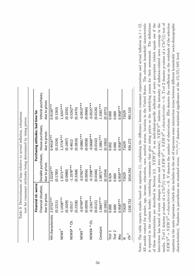
Table9:Determinantsofbiasrelativetoactualinflation,robustness

testforconsumerattitudesbeingdeterminedbyrisingprices.

Fina

ncia

l situ

atio

n,du

e to

 pric

esDu

rabl

e pu

rcha

ses,

due 

to p

rices

Hous

e pu

rcha

ses,

due 

to p

rices

Vehi

cle 

purc

hase

s,du

e to

 pric

es

HH c

hara

cter

istic

2.07

32**

*2.

0226

***

0.94

16**

*0.

9139

***

(0.1

211)

(0.1

785)

(0.1

524)

(0.1

263)

NEW

SP

1.14

38**

*1.

3571

***

1.27

76**

*1.

3247

***

(0.1

029)

(0.0

980)

(0.1

007)

(0.1

035)

NEW

SP *

 Ch.

­0.0

517

­1.1

078*

**­0

.461

2­0

.526

2**

(0.2

328)

(0.3

268)

(0.2

810)

(0.2

475)

NEW

SN

­0.0

749*

**­0

.078

2***

­0.0

881*

**­0

.091

3***

(0.0

059)

(0.0

056)

(0.0

058)

(0.0

060)

NEW

SN *

 Ch.

­0.1

261*

**­0

.159

8***

­0.0

668*

**­0

.052

5***

(0.0

121)

(0.0

166)

(0.0

142)

(0.0

126)

Cons

tant

1.06

67**

*1.

0871

***

1.18

81**

*1.

1581

***

(0.1

061)

(0.1

054)

(0.1

062)

(0.1

071)

Test

 10.

000

0.42

40.

002

0.00

0Te

st 2

0.00

00.

000

0.00

00.

000

Rho

0.95

8***

0.95

9***

0.95

8***

0.95

8***

N71

629

7162

971

629

7162

9Ch

i213

30.7

3210

14.5

9292

6.27

299

1.51

0

Fina

ncia

l sit.

 wor

sePu

rcha

sing

 att

itude

s: b

ad ti

me 

for

Notes:Thetablereportsresultsbasedonequation(1),explainingthedifferencebetweenconsumerexpectationsandactualinflationint+12.

Allmodelscontrolforgender,age,income,education,race,maritalstatus,locationintheUnitedStates.Therelevanthouseholdcharacteristic

isreportedinthecolumnheader,consideringconsumersthatgiverisingpricesastheunderlyingreasonfortheirassessment.Thedefinitions

ofthesecharacteristicsaredescribedinSection2.3.

NEWSPisan

individual-specificindicatorofnewsperception(whichequalsoneifthe

intervieweehasheardofrecentchangesinpricesandzerootherwise),NEWSNindexestheintensityofinflation-relatednewscoverageinthe

media.Test1denotesp-valuesofaChi2(1)testofNEWSP+NEWSP∗characteristic=0.Test2denotesp-valuesofaChi2(1)testof

NEWSN+NEWSN∗characteristic=0.Ndenotesthenumberofobservations.Rhodenotesthecoefficientontheresidualsoftheselection

equationinthemainregression(whichalsoincludesinthesetofregressorssomeinteractiontermsbetweendifferenthouseholds’socio-demographic

characteristics).Numbersinparenthesesarestandarderrors.***/**/*denotesstatisticalsignificanceatthe1%/5%/10%

level.

34

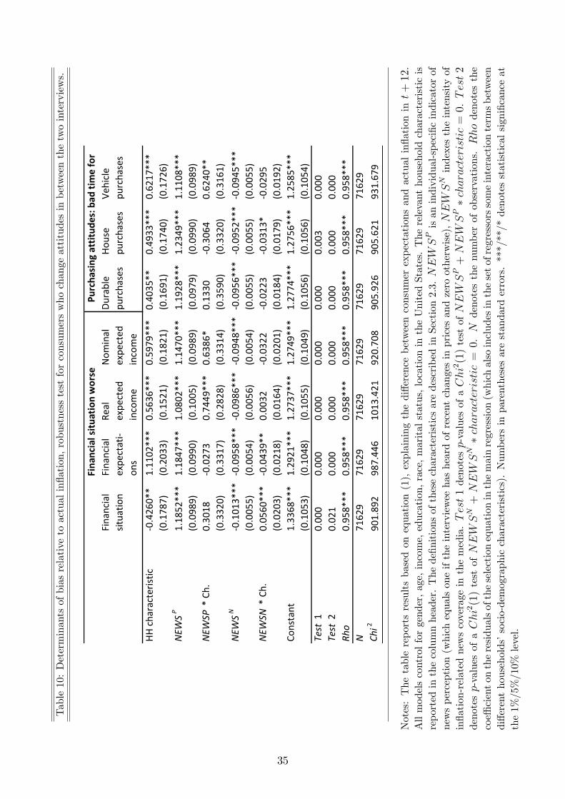
Table10:Determinantsofbiasrelativetoactualinflation,robustnesstestforconsumerswhochangeattitudesinbetweenthetwointerviews.

Fina

ncia

lsit

uatio

nFi

nanc

ial

expe

ctat

i­on

s

Real

expe

cted

inco

me

Nom

inal

expe

cted

inco

me

Dura

ble

purc

hase

sHo

use

purc

hase

sVe

hicl

epu

rcha

ses

HH c

hara

cter

istic

­0.4

260*

*1.

1102

***

0.56

36**

*0.

5979

***

0.40

35**

0.49

33**

*0.

6217

***

(0.1

787)

(0.2

033)

(0.1

521)

(0.1

821)

(0.1

691)

(0.1

740)

(0.1

726)

NEW

SP1.

1852

***

1.18

47**

*1.

0802

***

1.14

70**

*1.

1928

***

1.23

49**

*1.

1108

***

(0.0

989)

(0.0

990)

(0.1

005)

(0.0

989)

(0.0

979)

(0.0

990)

(0.0

989)

NEW

SP *

 Ch.

0.30

18­0

.027

30.

7449

***

0.63

86*

0.13

30­0

.306

40.

6240

**(0

.332

0)(0

.331

7)(0

.282

8)(0

.331

4)(0

.359

0)(0

.332

0)(0

.316

1)N

EWSN

­0.1

013*

**­0

.095

8***

­0.0

986*

**­0

.094

8***

­0.0

956*

**­0

.095

2***

­0.0

945*

**(0

.005

5)(0

.005

4)(0

.005

6)(0

.005

4)(0

.005

5)(0

.005

5)(0

.005

5)N

EWSN

 * C

h.0.

0560

***

­0.0

439*

*0.

0032

­0.0

322

­0.0

223

­0.0

313*

­0.0

295

(0.0

203)

(0.0

218)

(0.0

164)

(0.0

201)

(0.0

184)

(0.0

179)

(0.0

192)

Cons

tant

1.33

68**

*1.

2921

***

1.27

37**

*1.

2749

***

1.27

74**

*1.

2756

***

1.25

85**

*(0

.105

3)(0

.104

8)(0

.105

5)(0

.104

9)(0

.105

6)(0

.105

6)(0

.105

4)Te

st 1

0.00

00.

000

0.00

00.

000

0.00

00.

003

0.00

0Te

st 2

0.02

10.

000

0.00

00.

000

0.00

00.

000

0.00

0Rh

o0.

958*

**0.

958*

**0.

958*

**0.

958*

**0.

958*

**0.

958*

**0.

958*

**N

7162

971

629

7162

971

629

7162

971

629

7162

9Ch

i290

1.89

298

7.44

610

13.4

2192

0.70

890

5.92

690

5.62

193

1.67

9

Fina

ncia

l situ

atio

n w

orse

Purc

hasi

ng a

ttitu

des:

 bad

 tim

e fo

r

Notes:Thetablereportsresultsbasedonequation(1),explainingthedifferencebetweenconsumerexpectationsandactualinflationint+12.

Allmodelscontrolforgender,age,income,education,race,maritalstatus,locationintheUnitedStates.Therelevanthouseholdcharacteristicis

reportedinthecolumnheader.ThedefinitionsofthesecharacteristicsaredescribedinSection2.3.NEWSPisanindividual-specificindicatorof

newsperception(whichequalsoneiftheintervieweehasheardofrecentchangesinpricesandzerootherwise),NEWSNindexestheintensityof

inflation-relatednewscoverageinthemedia.Test1denotesp-valuesofaChi2(1)testofNEWSP+NEWSP∗characteristic=0.Test2

denotesp-valuesofaChi2(1)testofNEWSN+NEWSN∗characteristic=0.

Ndenotesthenumberofobservations.Rhodenotesthe

coefficientontheresidualsoftheselectionequationinthemainregression(whichalsoincludesinthesetofregressorssomeinteractiontermsbetween

differenthouseholds’socio-demographiccharacteristics).Numbersinparenthesesarestandarderrors.***/**/*denotesstatisticalsignificanceat

the1%/5%/10%

level.

35