Constraint Logic Programmingcliplab.org/~mcarro/Slides/CLP_Course/clp_course_3.pdfDifferences w.r.t. CPM (Critical Path Method): A particular application of ﬁnite domains Gives more

Constraint Logic Programming

Manuel [email protected]

Technical University of Madrid (Spain)

Manuel Carro — C.S. School — UPM – p.1/148

What is CLP


Constraints for Problem Solving

• Born within AI: e.g. house design

• Constraints as problem representationThe man in yellow does not have green eyesThe murderer knows no detective will ever wear darkclothes

• Need an appropriate constraint system (and solver)

• Solution: assignment which agrees with c initial constraintsMurderer: López, green eyes, Magnum gun

• Or, alternatively, constraints as problem solution(may express different solutions):

The murderer is one of those who had met the cabaretentertainer

• There might be no solution: Natural death


A General View• Ancestors: SKETCHPAD (1963), Waltz’s algorithm (1965?),

THINGLAB (1981), MACSYMA (1983)

• Constraints in logic languages:• Idea of Constraint Programming• General theory• In practice: based on Prolog + some constraint domain

• Constraints in imperative languages:• Equation solving libraries (ILOG)• Timestamping of variables:x := x + 1↔ xi := xi+1 + 1

• Constraints in functional languages:• Evaluation of expressions with free variables:• Absolute Set Abstraction


Constraints: High–level Problem Modelling

• Think of constraints as (dis)equations over arbitrary items

• Use constraint system primitives to encode the problemconditions• But:• Lack of modularity• Creating constraints dynamically not easy — must be statically

defined• Probably constraint system not powerful enough to reflect the

whole problem• Or solutions not given in the desired format


Programming:

• Use programming techniques:• Data structures and data abstraction• Ad–hoc algorithms, when desired / advantageous• Modularity

• Computational power: host language is enriched

• Set up constraints during program execution

• Possibility of adding control:• Data flow• Program execution• Constraint solving

• External communication


Logic

• Declarative reading:• Referential transparency• Small code units have their own, isolated meaning

(much like mathematical equations)

• Logical (mathematical) variables:• Bi–directional parameter passing

(more than pattern matching)• Single assignment• No need for explicit memory management• Data structures easy to build

• Non–determinism: built–in search procedure


Why Constraints and Programming?

• Constraints offer a powerful modeling tool

• But in real problems, there are. . .• . . . decisions which can be made in either way (and we do not

know before the right one) −→ search (also: disjunctiveconstraints)• . . . weak constraints which may or may not be satisfied• . . . an idea of the stages a task can be subdivided in• . . .

• Example: a program to help in house design

• Coupling constraint processing and programming gives morepower than any of them separately

• We know about programming; what is the deal with constraints?


Be a Solver (I)

D

E F

0

1 2 3

4

B C

1

0 G

A

• Assume the precedence net and tasklengths on the left

• The whole job must be finished in 10time units or less• Problem modelling:

a, b, c, d, e, f, g ∈ {0, . . . , 10}

a ≤ b, c, d

b + 1 ≤ ec + 2 ≤ e

c + 2 ≤ f

d + 3 ≤ f

e + 4 ≤ g

f + 1 ≤ g


Be a Solver (II)

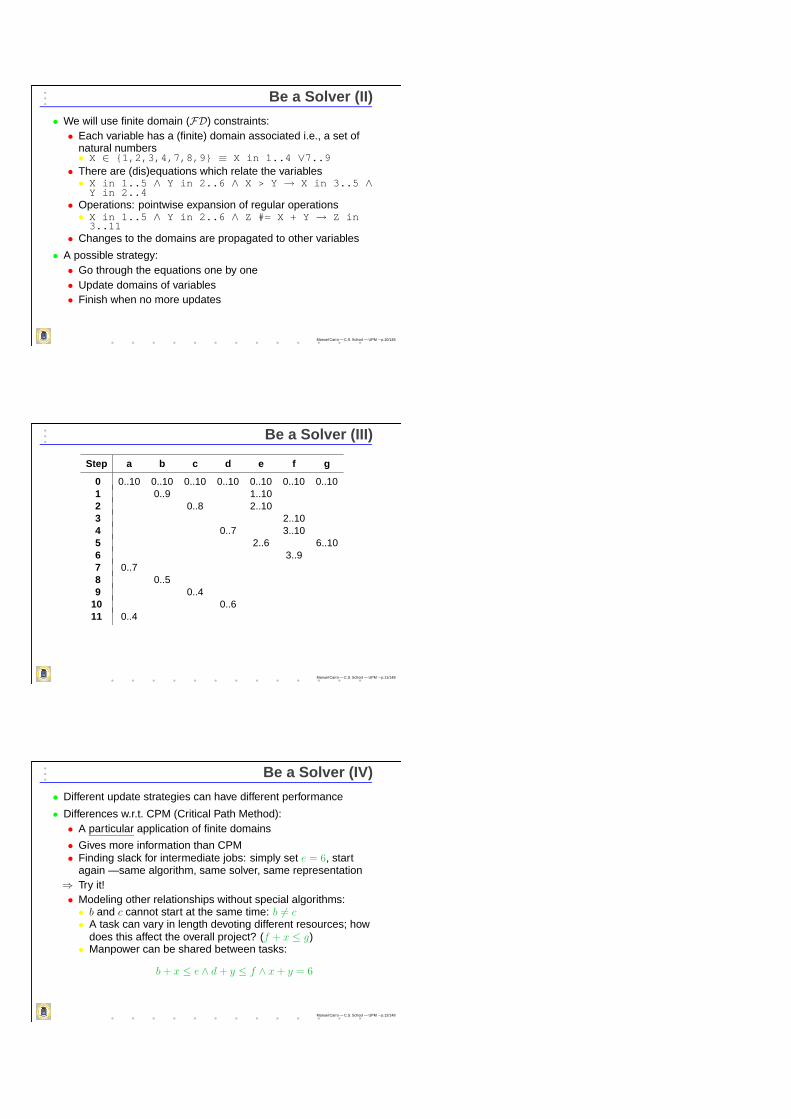
• We will use finite domain (FD) constraints:• Each variable has a (finite) domain associated i.e., a set of

natural numbers• X ∈ {1,2,3,4,7,8,9} ≡ X in 1..4 ∨7..9• There are (dis)equations which relate the variables• X in 1..5 ∧ Y in 2..6 ∧ X > Y → X in 3..5 ∧Y in 2..4

• Operations: pointwise expansion of regular operations• X in 1..5 ∧ Y in 2..6 ∧ Z #= X + Y → Z in3..11

• Changes to the domains are propagated to other variables

• A possible strategy:• Go through the equations one by one• Update domains of variables• Finish when no more updates


Be a Solver (III)

Step a b c d e f g

0 0..10 0..10 0..10 0..10 0..10 0..10 0..101 0..9 1..102 0..8 2..103 2..104 0..7 3..105 2..6 6..106 3..97 0..78 0..59 0..4

10 0..611 0..4


Be a Solver (IV)

• Different update strategies can have different performance

• Differences w.r.t. CPM (Critical Path Method):• A particular application of finite domains

• Gives more information than CPM• Finding slack for intermediate jobs: simply set e = 6, start

again — same algorithm, same solver, same representation⇒ Try it!• Modeling other relationships without special algorithms:• b and c cannot start at the same time: b 6= c• A task can vary in length devoting different resources; how

does this affect the overall project? (f + x ≤ g)• Manpower can be shared between tasks:

b + x ≤ e ∧ d + y ≤ f ∧ x + y = 6


Don’t Be a Solver• CLP languages provide built–in solvers

• For a variety of domains

• We will first briefly have a look at• Logical variables• Backtracking

using logic programming syntax

• Then we will merge it with constraint solving capabilities

• After this, we will look at Prolog, for practical reasons

• We will finish with a review of the operational model (andpragmatics)

• Everything spiced with examples and questions


A Basic Language


A Basic Constraint Language

• We will use a basic language whose components are:• Variables, starting with uppercase: X,Y, Speed

• Constants, either numbers or names starting with lowercase:1, 199, cat, a_dogThose constants are the Domain of the language• Atoms, which have the form p(X1, . . . , Xn), where:• p is the name of the atom, and n its arity (i.e. it admits n

arguments) — usually written p/n• X1, . . . , Xn are either constants or variables• Example:

hates(dog, cat)predates(big_fish, small_fish)

• Constraints: we will use only = /2 (syntactic equality)

• We will augment this language later


Clauses• A clause is a construction of the form p← b1, . . . , bn.

• p is an atom, each of b1, . . . , bn are either atoms or constraints

• Can be read as: p is true if b1, . . . , bn are all true

• p is termed as the head, and b1, . . . , bn as the body

• For convenience,← is often written as :-

• Example:animal(X):- X = dog.likes(C, F):- C = cat, F = fish.bigger(M1, M2):- M1 = men, M2 = mice.

• Meaning (under a particular interpretation):“dog” is an animal “cat” likes “fish”M1 is bigger than M2 if M1 equals “men” and M2 equals“mice” , or “men” are bigger than “mice”


Clauses (Cont.)

• Clauses can contain calls to user predicates

• Variables are used to pass arguments to them

• Example:eats(X, Y):- bigger(X, Y).pet(X):- animal(X), sound(X,Y), Y=bark.

• Interpretation:The big eat the small, orIf some X is bigger than some Y, then X eats Y

For X to be a pet, it must be an animal and the sound itproduces must be a bark , orIf X is and animal and X barks, then X is a pet, orA pet is an animal which barks


Implicit Equality

• Equality constraints are commonly written in a shorter form

• Ex.: p(X):- X = something. can be written asp(something).

• I.e., the symbol for the equality constraint does not appearexplicitly

• Thus, clauses likebigger(M1, M2):- M1 = men, M2 = mice.pet(X):- animal(X), sound(X, Y), Y = bark.

are commonly written asbigger(men, mice).pet(X):- animal(X), sound(X, bark).

with the same meaning as before


Facts• A fact is an expression of the form

p.

where p is an atom

• A fact is a clause without body (because the equality constraintsare implicitly understood)

• Its meaning is:the proposition (relationship) p always holds

• The following are facts:animal(dog).likes(cat, fish).bigger(men, mice).

• =/2 can also be defined (again) as =(X, X).


Predicates• A collection of clauses with the same head name• They represent different possibilities for something to be true

• Or, alternatively, different ways of accomplishing a task

• Example:pet(X):- animal(X), sound(X, bark).pet(X):- animal(X), sound(X, bubbles).

• Meaning:A pet is an animal which barks, or an animal which makesbubbles

• Variables in a clause are local to that clause (e.g., the Xs in thepredicate above)


Programs

• A program is a set of predicates

• Example:pet(X):- animal(X), sound(X, bark).pet(X):- animal(X), sound(X, bubbles).

animal(spot).animal(barry).animal(hobbes).

sound(spot, bark).sound(barry, bubbles).sound(hobbes, roar).

⇒ Introduce this program in a (C)LP compiler or interpreter, and playwith it (see the next slide)


Making Queries

• We interact with a logic program by making queries

• A query is a conjunction of atoms(which we want to be prove)

• An answer will consist of bindings for the variables in the querywhich make it true w.r.t. the program

• Several (different) answers are possible

• We will mark a query starting with ?-

• Example:?- sound(spot, X). ?- sound(A, roar).

X = bark A = hobbes?- animal(X). ?- animal(barry).

X = spot ; yesX = barry ; ?- sound(A, S).X = hobbes


Searching (I)

• Automatic search is performed through all paths given by theprogram

• Is pet(X) provable from the program, oris there any X such that it is a pet??- pet(X).

pet(X)

animal(spok) animal(barry) animal(hobbes)

animal(X), sound(X, bark) animal(X), sound(X, bubbles)

sound(barry, bubbles)animal(barry) animal(hobbes)animal(spok)sound(spok, bark)

(atoms inside boxes are conjunctions to prove/execute)

?- pet(hobbes).


Searching (Cont.)

• Searching allows finding all solutions to a query

• Backtracking is performed:• right to left, among goals• top to bottom, among clauses

(but other strategies also possible)?- pet(X), animal(Y).X = spot, Y = spot ;...X = barry, Y = hobbes

• After the first solution:• All possibilities for animal/1are tried in the same order as the

clauses in the program• Then the next clause for pet/1is tried• And so on, until all paths have been explored


Logical Variables

• Logical variables provide argument passing (to and frompredicates)

• And more interesting stuff (we will see later)

• Logical variable assignment is monotonic?- X = a.X = a?- X = a, X = b.no

• X cannot be at the same time a and b

• A hint as to why x := x + 1↔ xi := xi+1 + 1 in someimperative languages with constraints (first part of the lectures)


Logical Variables (Cont.)

• The constraint =/2 forces variables to have the same value — i.e.,they are unified

?- X = Y, X = a.X = a, Y = a.?- X = Y, pet(X), sound(Y, roars).no

⇒ (why?)?- X = Y, pet(X).X = spot, Y = spot;X = barry, Y = barry


Logical Variables (Contd.)

• Assume the following program:father_of(juan, pedro). father_of(juan, maria).father_of(pedro, miguel). mother_of(maria, david).grandfather_of(L,M):- father_of(L,N), father_of(N,M).grandfather_of(X,Y):- father_of(X,Z), mother_of(Z,Y).

⇒ Answer the questions:

?- father_of(juan, pedro).?- father_of(juan, david).?- father_of(juan, X).?- grandfather_of(X, miguel).?- grandfather_of(X, Y).?- X = Y, grandfather_of(X, Y).?- grandfather_of(X, Y), X = Y.

Write rules forgrandmother(X, Y)


The Execution Mechanism• Can also be seen as a tree traversal• Always select the leftmost goal

• Explore the search tree taking the leftmost unexplored branch,backtracking to explore later branches

grandparent(C,G):-parent(C,P), parent(P,G).

parent(C,P):- father(C,P).parent(C,P):- mother(C,P).

father(charles,philip).father(ana,george).

mother(charles,ana).

father(philip,X) mother(philip,X)

father(charles,P),parent(P,X)

parent(charles,P),parent(P,X)

grandparent(charles,X)

mother(charles.P),parent(P,X)

parent(ana,X)

failure

parent(philip,X)

failure X = george

father(ana,X) mother(ana,X)

failure


Database Programming: Electrical Circuits

Power

n1

n2

n3

n5n4

r1

r2t1

t2

t3

?- and_gate(In1,In2,Out).In1=n3, In2=n5, Out=n1

resistor(power,n1).resistor(power,n1).resistor(power,n2).transistor(n2,ground,n1).transistor(n3,n4,n2).transistor(n5,ground,n4).inverter(Input,Output):-

transistor(Input,ground,Output),resistor(power,Output).

nand_gate(Input1,Input2,Output):-transistor(Input1,X,Output),transistor(Input2,ground,X),resistor(power,Output).

and_gate(Input1,Input2,Output):-nand_gate(Input1,Input2,X),inverter(X, Output).


Datalog

• The basic language we have seen so far is a constraint languagewith:• Variables,• Constants (the domain of the constraint system),• Atoms (user predicates),• And a unique constraint = /2 which expresses equality

between constants or variables• There are no data structures• This language, plus numbers, some elementary arithmetic

operations, and some other facilities is named Datalog, and oftenused in deductive databases• Basic operations of relational databases easily expressed!


Datalog and the Relational DB Model

Traditional→ Codd’s Relational Model

File Relation TableRecord Tuple RowField Attribute Column

• Example:

Name Age SexBrown 20 MJones 21 FSmith 36 M

Person

Name Town YearsBrown London 15Brown York 5Jones Paris 21Smith Brussels 15Smith Santander 5

Lived–in

• The order of the rows is immaterial• (Duplicate rows are not allowed)


Datalog and the Relat. DB Model (Contd.)

Relat. Database → Logic Programming

Relation Name → Predicate symbolRelation → Predicate consisting of ground

facts (facts without variables)Tuple → Ground factAttribute → Argument of predicate

• Examples:

person(brown,20,male).person(jones,21,female).person(smith,36,male).

lived_in(brown,london,15).lived_in(brown,york,5).lived_in(jones,paris,21).lived_in(smith,brussels,15).lived_in(smith,santander,5).



• Union: r_union_s(X1,. . .,Xn) ←r(X1,. . .,Xn).r_union_s(X1,. . .,Xn) ←s(X1,. . .,Xn).

• Set Difference (discussion on negation postponed):r_diff_s(X1,. . .,Xn) ←r(X1,. . .,Xn),

not s(X1,. . .,Xn).r_diff_s(X1,. . .,Xn) ←s(X1,. . .,Xn),

not r(X1,. . .,Xn).

• Cartesian Product :r_X_s(X1,. . .,Xm,Xm+1,. . .,Xm+n) ←

r(X1,. . .,Xm), s(Xm+1,. . .,Xm+n).

• Projection: r13(X1,X3) ←r(X1,X2,X3).

• Selection:r_selected(X1,X2,X3) ←r(X1,X2,X3), ≤(X2,X3).



• Duplicates an issue: see “setof” later

• Deductive databases use these ideas to develop logic-baseddatabases• Often a subset of definite (Prolog) programs used (e.g.

“Datalog” – no data structures, no existential variables)• Variations of a “bottom-up” execution strategy used (instead of

the top-down, goal directed strategy shown here)• Formalization use the immediate consequence Tp operator to

compute a program model, restrict answers to the query


Adding Computation Domains:CLP Programs


What’s in a Domain• Informally, a computation domain for a constraint language

comprises:• A definition of the elements in the domain• Their interpretation,• The operations allowed among them, and• The interpretation of these operations

• Example:• We assumed a finite number of elements in the precedence

net example• A continuous set would not have allowed us to solve the

problem as we did


Different Constraint Domains: What for?• Why different computation domains?

• After all, everything is bytes...

• But:• Different problems and elements involved in them have

different characteristics• Some domains may be better suited for a given problem• And people do perceive different properties in the elements

around us• Having different domains allows us to:• Abstract the properties of the elements we are working with• Choose an appropriate constraint solver

• Thus, we do not have to deal with low–level details

• Example: having operations over complex numbers defined


Constraint Logic Programs

• We will show some examples of constraint logic programs

• We will use different constraint domains to highlight theircharacteristics• First we will present the characteristics of the domains and the

primitives used

• Then we will model (simple) problems and solve them using CLP


Equations in a Logic Language

• The CLP(<) language and system pioneered linear (dis)equationssolving together with a robust logic language

• CLP(<) featured an internal solver for linear equations, includingincremental solving thereof

• Equations represented directly as terms (i.e., as written down inpaper):?- X = 1 + Y - Z, X > Z, Z = Y + 3.

Y = Z - 3, X = -2, Z < -2

• Many other logic-based languages follow the same path: PrologII, Prolog III, Prolog IV, SICStus, Ciao Prolog, CHIP, CLP(FD), . . .


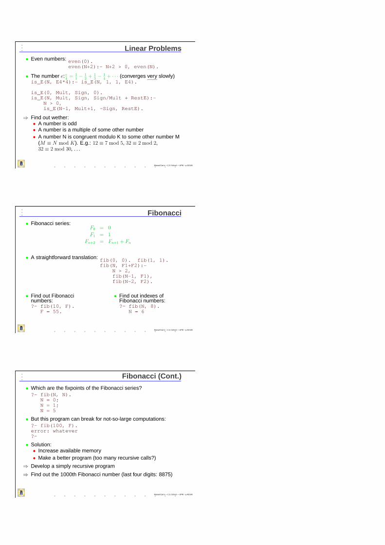
Linear (Dis)Equations

• A word of caution: syntax details may differ among differentimplementations

• We will augment the basic language with:• Floating point numbers: 4.0, 1e− 3

(they stand for the corresponding real numbers)• Arithmetic operators (+, ∗,−, /), with which we can construct

arithmetic terms: 3 + 4, X + 3 ∗ Y − Z/5These terms stand for arithmetic expressions• A predefined constraint = /2, which stands for arithmetic

equality (can also appear implicitly)• Some constraints which represent an order relation: >=/2, >/2,

=</2, </2

• We will augment the semantics of the language adding constraintsolving capabilities


Interacting

• Let us make some queries concerning linear arithmetic?- 4 - Y = 3.

Y = 1?- X = 3*Y - X/2, X+Y = Y - 4*X + 7.

Y = 7/10, X = 7/5.

• Sometimes giving a uniquely defined solution is not possible:?- X = Y + 3.

X = Y + 3

• The level of answer definiteness may differ amongimplementations:?- X >= Y, Y >= X.

X = Y?- X >= Y, Y >= X.

X - Y >= 0, Y - X >= 0

• (Both are correct, though)


Linear Problems• The folowing simple, recursive program defines the natural

numbers:nat(0).nat(N):- N > 0, nat(N-1).

(zero is a natural number, and a number greater than zero is alsoa natural number, provided that its predecessor is a naturalnumber)

?- nat(X).X = 0 ;X = 1 ;X = 2 ;

?- nat(3.4).false

?- nat(-8).false


Linear Problems• Even numbers: even(0).

even(N+2):- N+2 > 0, even(N).

• The number e: e4

= 1

1− 1

2+ 1

3− 1

4+ · · · (converges very slowly)

is_E(N, E4*4):- is_E(N, 1, 1, E4).

is_E(0, Mult, Sign, 0).is_E(N, Mult, Sign, Sign/Mult + RestE):-

N > 0,is_E(N-1, Mult+1, -Sign, RestE).

⇒ Find out wether:• A number is odd• A number is a multiple of some other number• A number N is congruent modulo K to some other number M

(M ≡ N mod K). E.g.: 12 ≡ 7 mod 5, 32 ≡ 2 mod 2,32 ≡ 2 mod 30, . . .


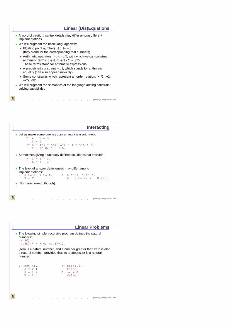
Fibonacci• Fibonacci series:

F0 = 0

F1 = 1

Fn+2 = Fn+1 + Fn

• A straightforward translation: fib(0, 0). fib(1, 1).fib(N, F1+F2):-

N > 2,fib(N-1, F1),fib(N-2, F2).

• Find out Fibonaccinumbers:?- fib(10, F).

F = 55.

• Find out indexes ofFibonacci numbers:?- fib(N, 8).

N = 6


Fibonacci (Cont.)

• Which are the fixpoints of the Fibonacci series??- fib(N, N).

N = 0;N = 1;N = 5

• But this program can break for not-so-large computations:?- fib(100, F).error: whatever?-

• Solution:• Increase available memory• Make a better program (too many recursive calls?)

⇒ Develop a simply recursive program

⇒ Find out the 1000th Fibonacci number (last four digits: 8875)


Finite Domains• Another interesting domain is that of finite domains

• The solver associates to each variable a set of numbers, usuallydrawn from the naturals• The (linear) constraint symbols we have seen are extended to

work with finite domains• Operations are pointwise extensions of the corresponding ones in

numbers• We will assume the right semantics and behavior is deduced from

the context and variables


Examples of FD Arithmetic?- X = A + B, A in 1..3, B in 3..7.

B in 3..7, A in 1..3, X in 4..10.

• The respective minima and maxima are added?- X = A - B, A in 1..3, B in 3..7.

B in 3..7, A in 1..3, X in -6..0.

• The minimum value of X is the minimum value of A minus themaximum value of B• (Similar for the maximum values)

• Putting more constraints:?- X = A - B, A in 1..3, X => 0, B in 3..7.

B = 3, A = 3, X = 0.


Some Useful Primitives• Being able to access the bounds of a variable is useful

• fd_min(X, T): T is the minimum value in the domain of thevariable X (resp. fd_max/2)

• This can be used to minimize (c.f., maximize) a solution?- X = A - B, A in 1..3, B in 3..7, fd_min(X,X).

B = 7, A = 1, X = -6

• Not accurate: propagation-generated domains are upper bounds

• We will come to this later


Limits of FD arithmetics• FD constraints are (partially) solved by means of propagation

• A counterpart of algebraic manipulation

• Propagation is a deterministic procedure — does not performsearch• This is necessarily not complete:• No restriction on what equations can be written• Inexistence of general solving methods for, e.g., polinomials of

degree 5 (and above)

• Fortunately, the FD domain is finite and discrete


Enumeration Primitives• A family of predicates enumerate the values of a variable’s

domain→ causes further simplificationslabeling(Var)• instantiates Var to all the values in its domain• Usually available also aslabeling(ListOfVars)(straightforward to implement)?- Num=1001, Num = A * B, A in 1..Num,

B in 1..A, labeling([A, B]).B = 1, A = 1001, Num = 1001;B = 7, A = 143, Num = 1001;B = 11, A = 91, Num = 1001;B = 13, A = 77, Num = 1001

⇒ Try with bigger numbers, and interchanging the order of theenumeration. Is there any difference? Why?


A Project Management Problem (I)

D

E F

0

1 2 3

4

B C

1

0 G

A

• The job whose dependencies and tasklengths are shown at the left should befinished in 10 time units or less

• Constraints:pn1(A, B, C, D, E, F, G):-

A >= 0, G =< 10,B >= A, C => A, D >= A,E >= B + 1, E >= C + 2,F >= C + 2, F >= D + 3,G >= E + 4, G >= F + 1.


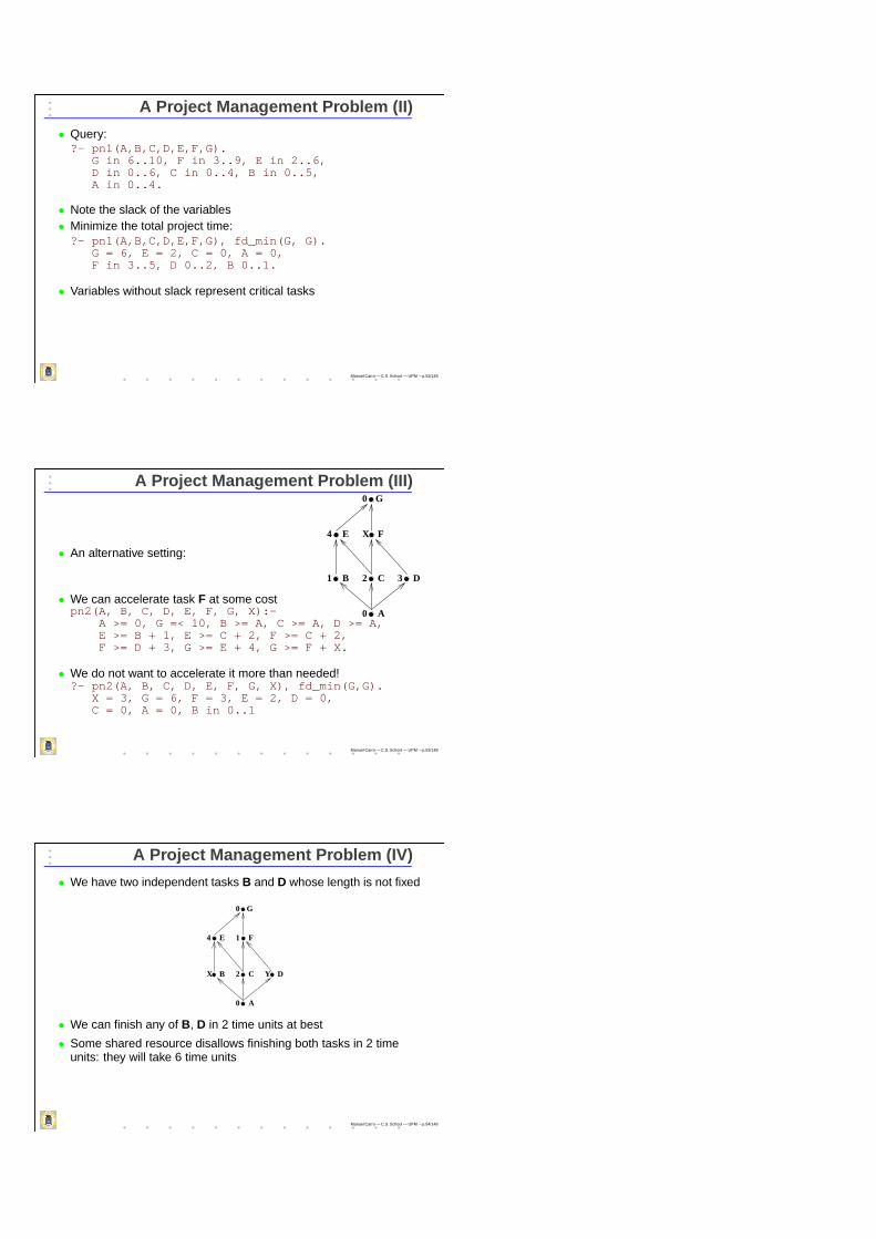
A Project Management Problem (II)

• Query:?- pn1(A,B,C,D,E,F,G).

G in 6..10, F in 3..9, E in 2..6,D in 0..6, C in 0..4, B in 0..5,A in 0..4.

• Note the slack of the variables• Minimize the total project time:?- pn1(A,B,C,D,E,F,G), fd_min(G, G).

G = 6, E = 2, C = 0, A = 0,F in 3..5, D 0..2, B 0..1.

• Variables without slack represent critical tasks


A Project Management Problem (III)

• An alternative setting:

D

E F

0

1 2 3

4

B C

0 G

A

X

• We can accelerate task F at some costpn2(A, B, C, D, E, F, G, X):-

A >= 0, G =< 10, B >= A, C >= A, D >= A,E >= B + 1, E >= C + 2, F >= C + 2,F >= D + 3, G >= E + 4, G >= F + X.

• We do not want to accelerate it more than needed!?- pn2(A, B, C, D, E, F, G, X), fd_min(G,G).

X = 3, G = 6, F = 3, E = 2, D = 0,C = 0, A = 0, B in 0..1


A Project Management Problem (IV)

• We have two independent tasks B and D whose length is not fixed

D

E F

0

2B C

0 G

A

1

Y

4

X

• We can finish any of B, D in 2 time units at best

• Some shared resource disallows finishing both tasks in 2 timeunits: they will take 6 time units


A Project Management Problem (V)

• Constraints describing the net:pn3(A, B, C, D, E, F, G, X, Y):-

A >= 0, G =< 10, X >= 2, Y >= 2, X + Y = 6,B >= A, C >= A, D >= A, E >= B + X, E >= C + 2,F >= C + 2, F >= D + Y, G >= E + 4, G >= F + 1.

• Query:?- pn3(A,B,C,D,E,F,G,X,Y), fd_min(G,G).

Y = 4, X = 2, G = 6, E = 2, C = 0, B = 0,A = 0, F in 4..5, D in 0..1

• I.e., we must devote more resources to task X

• All tasks but F and D are critical now


Minimization• In some cases, fd_min/2 (c.f., fd_max/2) is not enough to

provide the best solution

• For example, when (incomplete) propagation is unable to find outthe tighter bounds?- X in 0..1, Z = X*X, Z \= X, fd_max(Z, W).

W = 1, X in 0..1, Z in 0..1

• Propagation should not prune more than strictly necessary(risk of missign solutions!)• It may prune less than possible→ consistency algorithms

• A labeling + branch–and–bound procedure is usually provided:?- pn3(A,B,C,D,E,F,G,X,Y),

minimize(labeling(G),G).


Other Constraints and Operations

• CLP(FD) systems usually include several more constraintoperations / relationship primitives:• Disjoint intervals: A in 1..3 \/ 5..9

• Boolean pseudo-operations (based, e.g., on specializing FD to0..1)• Arbitrary operations (suspended until propagation /

enumeration takes place)• Reification: C \#<=> B(C constraint, B variable):• C posted if B = 1• ¬C posted if B = 0• B = 0 if C entailed• B = 1 if C disentailed• Raises the question of negation and negation in the realm of

constraints


Herbrand Terms• Our last example will be Herbrand terms

• Herbrand terms, or finite trees, are the non-interpreted functionsof first-order logic

• In a logic language, they are very useful to build data structures


Herbrand Terms (Cont)

• Herbrand terms are defined as:• A variable is a Herbrand term• A constant is a Herbrand term• A functor f with arity n applied to n

terms is a Herbrand term:f(t1, t2, . . . tn)

• Herbrand terms are a representation oftrees:• Variables are open leaves• Constants are fully instantiated leaves• Function symbols are nodes

• Example: f(a,X, g(Y, t)) represents thetree on the right

f

X g

Y t

a


Herbrand Terms: Syntactic Equality

• The only constraint allowed between Herbrand terms is =/2

• Its meaning is syntactic equality (unification)

• Roughly speaking:• An equation f(t1, . . . , tn) = f(u1, . . . , un) is solved by solving

t1 = u1, . . . , tn = un

• An equation v = t, where v is a variable and t is a term whichdo not contains v is solved with the binding v/t

• Equations like t = t can be deleted• If none of the above can be applied, the initial terms cannot be

unified• Examples: ?- X = f(T, a), T = b.

T = b, X = f(b,a)?- f(X, g(X, Y), Y) = f(a, T, b).

X = a, Y = b, T = g(a, b)


Structured Data and Data Abstraction• Data structures are created using terms:course(comp_logic, mond, 19, 21,

’Manuel’, ’Carro’, new, 1302).

• When is the Computational Logic course??- course(comp_logic,Day,Start,End,C,D,E,F).

• Structured version:course(comp_logic, When, Lecturer, Location):-

When = hour(mond,19,21),Lecturer = lecturer(’Manuel’,’Hermenegildo’),Location = location(new,1302).

• When is the Computational Logic course??- course(comp_logic, When, A, B).


Constructing Data Structures

• Functors can be thought of as representing non–interpretedfunctions (i.e., records)

• The main application of functors is as data structure constructors

• Sample program, step by step

• We have a small database of people who are friends:

friends(peter, mark).friends(anna, marcia).friends(anna, luca).

?- friends(anna, X).X = marcia ;X = luca

?- friends(X, anna).no

• No friends?


Constructing Data Structures (Cont.)

• Being friends is symmetric:are_friends(A, B):- friends(A, B).are_friends(A, B):- friends(B, A).

?- are_friends(anna, X).X = marcia ;X = luca

?- are_friends(X, anna).X = marcia ;X = luca

• Some of our friends are married:married(couple(peter, anna)).married(couple(mark, kathleen)).married(couple(alvin, marcia)).

• Note that married defines couples of persons?- married(A).

A = couple(peter,anna) ;A = couple(mark,kathleen) ;A = couple(alvin,marcia)



• We may want to know who is spouse of who?- married(couple(peter, S)).

S = anna?- married(couple(marcia, S)).

no

• Argument order matters, of course

• We must specify what is a spousespouse(couple(A, B), A).spouse(couple(A, B), B).

• Then we can forget about the order

?- spouse(C, peter),married(C).C = couple(peter,anna)

?- married(C),spouse(C, marcia).C = couple(alvin,marcia)



• Some couples go out for dinner if...go_out_for_dinner(Ma, Mb):-

married(Ma),married(Mb),spouse(Ma, A),spouse(Mb, B),are_friends(A, B).

?- go_out_for_dinner(A, B).A=couple(peter,anna), B=couple(mark,kathleen) ;A=couple(peter,anna), B=couple(alvin,marcia) ;A=couple(mark,kathleen), B=couple(peter,anna) ;A=couple(alvin,marcia), B=couple(peter,anna)}


Structuring Old Problems

resistor(r1,power,n1). transistor(t1,n2,ground,n1).resistor(r2,power,n2). transistor(t2,n3,n4,n2).

transistor(t3,n5,ground,n4).

inverter(inv(T,R),Input,Output) :-transistor(T,Input,ground,Output),resistor(R,power,Output).

nand_gate(nand(T1,T2,R),Input1,Input2,Output) :-transistor(T1,Input,X,Output),transistor(T2,Input2,ground,X),resistor(R,power,Output).

and_gate(and(N,I),Input1,Input2,Output) :-nand_gate(N,Input1,Input2,X),inverter(I,X).

?- and_gate(G,In1,In2,Out).G=and(nand(t2,t3,r2), inv(t1,r1)), In1=n3, In2=n5, Out=n1


Constructing Recursive Data Structures

• Functors allow constructing recursive data structures

• Simplest recursive data structure: Peano natural numbers• z is a Peano number (meaning zero, 0)• s(N) is a Peano number if N is a Peano number

(meaning the successor of N , i.e., N + 1)

• Logic characterization of Peano numbers:natural(z).natural(s(N)):- natural(N).

• Note: very similar to the constraint program


Constructing Recursive Data Structures (Cont.)?- natural(z).

yes?- natural(potato).

no?- natural(s(s(s(z)))).

yes?- natural(X).

X = z ;X = s(z) ;X = s(s(z));...

?- natural(s(s(X))).X = z ;X = s(z) ;X = s(s(z));


Constructing Recursive Data Structures (Cont.)

• Addition:plus(z, X, X):- natural(X).plus(s(N), X, s(Y)):- plus(N, X, Y).

• Some queries:?- plus(s(s(z)), s(z), R).

R = s(s(s(z)))?- plus(s(s(s(z))), T, s(s(s(s(s(z))))).

T = s(z)?- plus(s(s(s(s(z)))), T, s(s(s(z)))).

no?- plus(X, Y, s(s(z))).

X = z, Y = s(s(z)) ;X = s(z), Y = s(z) ;X = s(s(z)), Y = z}


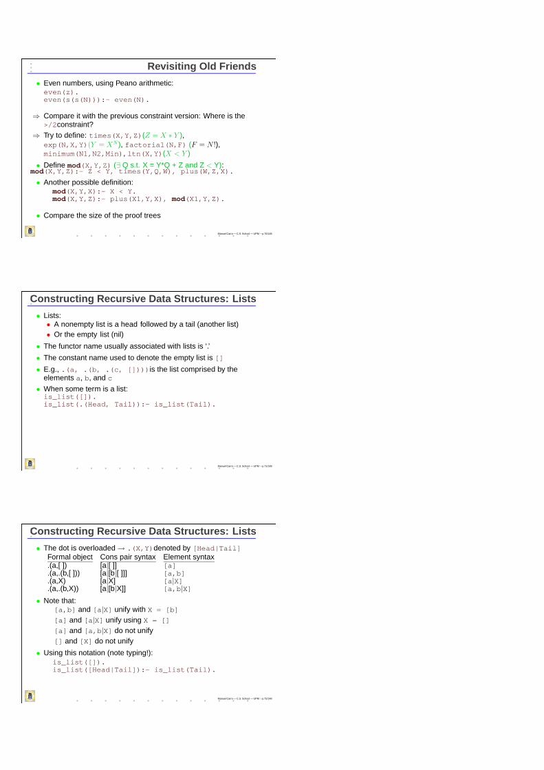
Revisiting Old Friends

• Even numbers, using Peano arithmetic:even(z).even(s(s(N))):- even(N).

⇒ Compare it with the previous constraint version: Where is the>/2constraint?

⇒ Try to define: times(X,Y,Z)(Z = X ∗ Y ),exp(N,X,Y)(Y = XN ), factorial(N,F) (F = N !),minimum(N1,N2,Min), ltn(X,Y)(X < Y )

• Define mod(X,Y,Z) (∃ Q s.t. X = Y*Q + Z and Z < Y):mod(X,Y,Z):- Z < Y, times(Y,Q,W), plus(W,Z,X).

• Another possible definition:mod(X,Y,X):- X < Y.mod(X,Y,Z):- plus(X1,Y,X), mod(X1,Y,Z).

• Compare the size of the proof trees


Constructing Recursive Data Structures: Lists

• Lists:• A nonempty list is a head followed by a tail (another list)• Or the empty list (nil)

• The functor name usually associated with lists is ‘.’

• The constant name used to denote the empty list is []

• E.g., .(a, .(b, .(c, [])))is the list comprised by theelements a, b, and c

• When some term is a list:is_list([]).is_list(.(Head, Tail)):- is_list(Tail).


Constructing Recursive Data Structures: Lists

• The dot is overloaded→ .(X,Y)denoted by [Head|Tail]Formal object Cons pair syntax Element syntax.(a,[ ]) [a|[ ]] [a].(a,.(b,[ ])) [a|[b|[ ]]] [a,b].(a,X) [a|X] [a|X].(a,.(b,X)) [a|[b|X]] [a,b|X]

• Note that:[a,b] and [a|X] unify with X = [b]

[a] and [a|X] unify using X = []

[a] and [a,b|X] do not unify[] and [X] do not unify

• Using this notation (note typing!):is_list([]).is_list([Head|Tail]):- is_list(Tail).


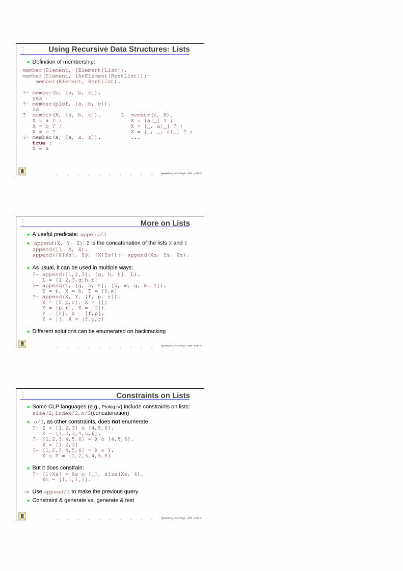
Using Recursive Data Structures: Lists

• Definition of membership:

member(Element, [Element|List]).member(Element, [AnElement|RestList]):-

member(Element, RestList).

?- member(b, [a, b, c]).yes

?- member(plof, [a, b, c]).no

?- member(X, [a, b, c]). ?- member(a, X).X = a ? ; X = [a|_] ? ;X = b ? ; X = [_, a|_] ? ;X = c ? X = [_, _, a|_] ? ;

?- member(a, [a, X, c]). ...true ;X = a


More on Lists• A useful predicate: append/3

• append(X, Y, Z): Z is the concatenation of the lists X and Yappend([], X, X).append([X|Xs], Ys, [X|Zs]):- append(Xs, Ys, Zs).

• As usual, it can be used in multiple ways:?- append([1,2,3], [g, h, t], L).

L = [1,2,3,g,h,t]?- append(T, [g, h, t], [0, m, g, X, Y]).

Y = t, X = h, T = [0,m]?- append(X, Y, [f, p, r]).

Y = [f,p,r], X = [];Y = [p,r], X = [f];Y = [r], X = [f,p];Y = [], X = [f,p,r]

• Different solutions can be enumerated on backtracking


Constraints on Lists• Some CLP languages (e.g., Prolog IV) include constraints on lists:size/2, index/2, o/3(concatenation)

• o/3, as other constraints, does not enumerate?- Z = [1,2,3] o [4,5,6].

Z = [1,2,3,4,5,6].?- [1,2,3,4,5,6] = X o [4,5,6].

X = [1,2,3]?- [1,2,3,4,5,6] = X o Y.

X o Y = [1,2,3,4,5,6]

• But it does constrain:?- [1|Xs] = Xs o [_], size(Xs, 4).

Xs = [1,1,1,1].

⇒ Use append/3 to make the previous query

• Constraint & generate vs. generate & test


Recursive Programming: Lists (Contd.)

• reverse(Xs,Ys): Ys is the list obtained by reversing theelements in the list Xs. For each element X of Xs, put X at the endof the rest of the Xs list already reversed:reverse([X|Xs],Ys ):-

reverse(Xs,Zs), append(Zs,[X],Ys).

• How can we stop? reverse([],[]).

• As defined, reverse(Xs,Ys) is very inefficient (why?)

• Another possible definition would be:reverse(Xs,Ys):- reverse(Xs,[],Ys).reverse([],Ys,Ys).reverse([X|Xs],Acc,Ys):- reverse(Xs,[X|Acc],Ys).

⇒ Find efficiency differences between these two versions


Problems on Lists• Lists: the most widely used data structures in (C)LP

• Write definitions for the following predicates (use Peano):⇒ len(N, L): N is the length of L⇒ suffix(S, L): S is a suffix of L⇒ prefix(P, L): P is a prefix of L⇒ sublist(S, L): S is a sublist of L⇒ last(E, L) E is the last element of L⇒ palindrome(L): L is a palindrome⇒ evenodd(L, E, O): E is the list of elements in even position

in L and O is the list of the elements in odd position⇒ select(E, L1, L2): L2 is L1 without the element E, e.g.,

?- select(X, [a,c,n], L).L = [c, n], X = a ;L = [a, n], X = c ;L = [a, c], X = n


Constructing Recursive Data Structures: Trees

• A binary tree with a piece of information in each node

• Use, for example, the functor tree/3• Its first argument is the item of information• The second and third ones are the left and right sons

(subtrees)• Use the constant void for empty treesis_tree(void).is_tree(tree(Info, Left, Right):-

is_tree(Left), is_tree(Right).

• Membership:tree_member(Element, tree(Element, L, R)).tree_member(Element, tree(E, L, R)):-

tree_member(Element, L).tree_member(Element, tree(E, L, R)):-

tree_member(Element, R).


Recursive Data Structures: Trees• pre_order(Tree,Order): Order is a list containing all the

elements in Tree in preorderpre_order(void,[]).pre_order(tree(X,Left,Right),Order):-

pre_order(Left,OrdLft),pre_order(Right,OrdRght),append([X|OrdLft],OrdRght,Order).

⇒ Define:• in_order(Tree,Order)• post_order(Tree,Order)


Manipulating Symb. Expressions

• Towers of Hanoi• Only one disk can be moved at a time

• Larger disks can never be placed on top of a smaller disks

• The predicate is hanoi(N,A,B,C,Moves)

• Moves: sequence of moves from peg A to peg B using peg C asauxiliary

• Each functor move(A, B) represents that the top disk in A goesto B.hanoi(s(0),A,B,C,[move(A, B)]).hanoi(s(N),A,B,C,Moves):-

hanoi(N,A,C,B,M1),hanoi(N,C,B,A,M2),append(M1,[move(A, B)|M2],Moves).


Manipulating Symb. Expressions (Contd.)

Recognize the sequence ofcharacters accepted by the fol-lowing non-deterministic, finiteautomaton (NDFA) at the right,where q0 is the initial and finalstate

q0 q1

a

b

b

• Strings represented as a list of constantsinitial(q0). final(q0).delta(q0,a,q1). delta(q1,b,q0). delta(q1,b,q1).

accept(S):- initial(Q), accept(Q,S).accept(Q,[]):- final(Q).

accept(Q,[X|Xs]):- delta(Q,X,NewQ), accept(NewQ,Xs).


CLP in Practice• Usual CLP systems include Herbrand terms (the primary Prolog

constraint system)

• In fact, usually built as extended Prolog systems

• Thus, they inherit all Prolog capabilities

• Plus the added power and flexibility of constraints

• A big advantage: mixing several constraint systems in the sameprogram

• Communication among solvers a problem

• Typing also an issue

• Some allow the user to define user constraints (and evenconstraint solvers→ CHR)

• Herbrand terms + a constraint system: common combination


Linear Equations

• Vector × vector multiplication (dot product):

· : <n ×<n −→ <(x1, x2, . . . , xn) · (y1, y2, . . . , yn) = x1 · y1 + · · · + xn · yn

• Vectors represented as lists of numbersprod([], [], 0).prod([X|Xs], [Y|Ys], X * Y + Rest):-

prod(Xs, Ys, Rest).

?- prod([2, 3], [4, 5], K).K = 23

?- prod([2, 3], [5, X2], 22).X2 = 4


Analog RLC circuits

• Analysis and synthesis of analog circuits in steady state

• Each circuit is composed either of a simple component, or aconnection of simpler circuits

• We will assume subnetworks connected only in parallel andseries −→ Ohm laws will suffice• Relate current (I), voltage (V) and frequency (W) in steady state

• Entry point circuit(C, V, I, W): across the network C, thevoltage is V, the current is I and the frequency is W

• V and I must be modeled as complex numbers (the imaginarypart takes into account the angular frequency)

• Herbrand terms used to provide data structures


Analog RLC circuits (Cont.)

• Complex number X + Y i modeled as c(X, Y)

• Basic operations:c_add(c(Re1,Im1), c(Re2,Im2), R):-

R = c(Re1+Re2,Im1+Im2).c_mult(c(Re1,Im1),c(Re2,Im2),c(Re3,Im3)):-

Re3 = Re1 * Re2 - Im1 * Im2,Im3 = Re1 * Im2 + Re2 * Im1.

• Circuits in series:circuit(series(N1, N2), V, I, W):-

c_add(V1, V2, V),circuit(N1, V1, I, W), circuit(N2, V2, I, W).

• Circuits in parallel:circuit(parallel(N1, N2), V, I, W):-

c_add(I1, I2, I),circuit(N1, V, I1, W), circuit(N2, V, I2, W).


Analog RLC circuits (Cont.)

Basic components modeled as a separate units:

• Resistor: V = I ∗ (R + 0i)circuit(resistor(R), V, I, W):-

c_mult(I, c(R, 0), V).

• Inductor: V = I ∗ (0 + WLi)circuit(inductor(L), V, I, W):-

c_mult(I, c(0, W * L), V).

• Capacitor: V = I ∗ (0− 1

WCi)

circuit(capacitor(C), V, I, W):-c_mult(I, c(0, -1 / (W * C)), V).

I = 0.065

L = 0.00073

C = ?R = ?

V = 2500

ω = 2400

?- circuit(parallel(inductor(0.073),series(capacitor(C),

resistor(R))),c(4.5, 0), c(0.65, 0), 2400).

R = 24939720/3608029,C = 3608029/2365200000.


Summarizing

• In general:• Data structures (Herbrand terms) for free• Logical variables may have constraints associated to it

• Problem modeling :• Rules represent the problem at a high level• Program structure, modularity• Recursion used to set up constraints• Constraints encode problem conditions• Solutions also expressed as constraints

• Combinatorial search problems:• Backtracking makes enumeration easy• Constraints help keep the search space manageable


Logic Programming: Prolog

• CLP over Herbrand terms is classically referred to as LogicProgramming

• The programming language Prolog is based on logicprogramming ideas, plus:• Fixed evaluation rules (left–to–right, depth–first)• Numerous builtins (input/output, execution control,

meta–logic...)• Interfacing with external language libraries• Efficient implementations• . . . and much more

• Prolog can be used advantageously for programming symbolic,complex applications

• Virtually, all modern Prolog implementations provide some sort ofconstraint capabilities (other than Herbrand terms)


Semantics of CLP Programs


Basic Operations on Constraints

• D an structure (an interpretation of the symbols of a signature)

• Constraint domains expected to support some basic operations

1. Consistency (or satisfiability) test: D |= ∃c,2. Implication or entailment: D |= c0 → c1,3. Projection of a constraint c0 onto variables x to obtain a

constraint c1 such that D |= c1 ↔ ∃−xc0,4. Detection of uniqueness of variable value:D |= c(x, z) ∧ c(y, w)→ x = y

• Actually, only the first one is really required

• In actual implementations, some of these operations—inparticular the test of consistency—may be incomplete


Basic Operations (II)

• Examples:• x ∗ x < 0 is inconsistent in < (because ¬∃x ∈ < : x ∗ x < 0)• D |= (x ∧ y = 1)→ (x ∨ y = 1) in BOOL• In FT , the projection of x = f(y) ∧ y = f(z) on {x, z} is

x = f(f(z))

• InWE , D |= x · a · x = x · a ∧ y · b · y = y · b→ x = y

• Prove the last assertion!


Properties of CLP Languages

• T axiomatizes some of the properties of D

• For a given Σ, let (D,L) be a constraint domain with signature Σ,and T a Σ–theory.

• D and T correspond on L if:• D is a model of T , and

• for every constraint c ∈ L, D |= ∃c iff T |= ∃c.

• T is satisfaction complete with respect to L if for every constraintc ∈ L, either T |= ∃c or T |= ¬∃c.

• (D,L) is solution compact if

∀c∃{ci}i∈I : D |= ∀x¬c(x)←→∨

i∈I

ci(x)

i.e., any negated constraint in L can be expressed as a (in)finitedisjunction of constraints


Solution Compactness

• Important to lift SLDNF results to CLP(X )

• We have to deal only with user predicates

• E.g.• x 6≥ y in CLP(<) is x < y

• x 6= y in CLP(<) is x < y ∨ y < x

• <Lin with constraint x 6= π is not s.c.

• How can we express x 6= y in CLP(FT )?


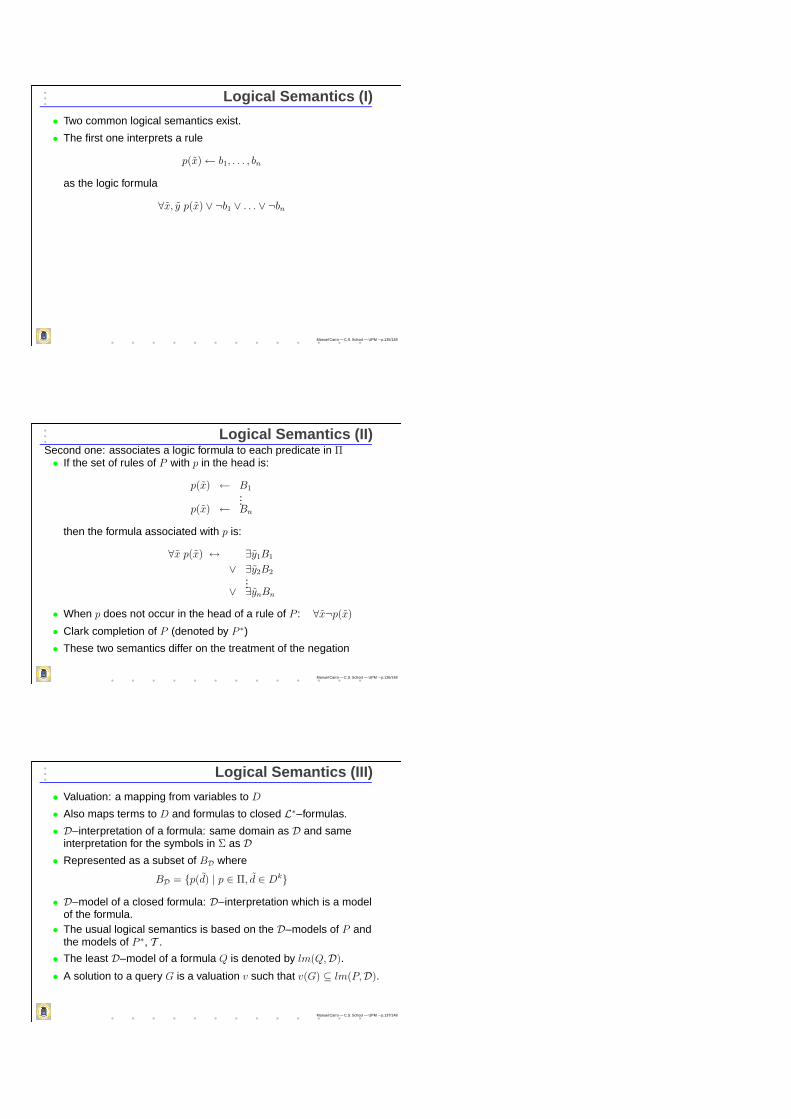
Logical Semantics (I)

• Two common logical semantics exist.

• The first one interprets a rule

p(x)← b1, . . . , bn

as the logic formula

∀x, y p(x) ∨ ¬b1 ∨ . . . ∨ ¬bn


Logical Semantics (II)Second one: associates a logic formula to each predicate in Π• If the set of rules of P with p in the head is:

p(x) ← B1

...p(x) ← Bn

then the formula associated with p is:

∀x p(x) ↔ ∃y1B1

∨ ∃y2B2...

∨ ∃ynBn

• When p does not occur in the head of a rule of P : ∀x¬p(x)

• Clark completion of P (denoted by P ∗)

• These two semantics differ on the treatment of the negation


Logical Semantics (III)

• Valuation: a mapping from variables to D

• Also maps terms to D and formulas to closed L∗–formulas.

• D–interpretation of a formula: same domain as D and sameinterpretation for the symbols in Σ as D

• Represented as a subset of BD where

BD = {p(d) | p ∈ Π, d ∈ Dk}

• D–model of a closed formula: D–interpretation which is a modelof the formula.• The usual logical semantics is based on the D–models of P and

the models of P ∗, T .

• The least D–model of a formula Q is denoted by lm(Q,D).

• A solution to a query G is a valuation v such that v(G) ⊆ lm(P,D).


Fixpoint Semantics

• Based on one-step consequence operator TDP (also called

“immediate consequence operator”).

• Take as semantics lfp(TDP ), where:

TD

P (I) = {p(d) | p(x)← c, b1, . . . , bn ∈ P, ai ∈ I,

D |= v(c), v(x) = d, v(bi) = ai}

• Theorems:1. TD

P ↑ ω = lfp(TDP )

2. lm(P,D) = lfp(TDP )


Top–Down Operational Semantics (I)• General framework, formalized as a transition system

• State: a 3–tuple 〈A,C, S〉, or fail, where• A is a multiset of atoms and constraints,• C

⋃

S multiset of constraints,• C, active constraints (awake)• S, passive constraints (asleep)

• Computation and selection rules depend on A

• Transition system: parameterized by a predicate consistent and afunction infer:• consistent(C) checks the consistency of a constraint store

• Usually “consistent(C) iff D |= ∃c”, but sometimes “if D |= ∃cthen consistent(C)”• infer(C, S) computes a new set of active and passive

constraints


Top–Down Operational Semantics (II)• Transition r: rewriting using user predicates〈A

⋃

a, C, S〉 →r 〈A⋃

B,C, S⋃

(a = h)〉if h← B ∈ P , and a and h have the same predicate symbol, or〈A

⋃

a, C, S〉 →r failif there is no rule h← B of P such that a and h have the samepredicate symbol (a = h is a set of argument–wise equations) if ais a predicate symbol selected by the computation rule

• Transition c: selects constraints 〈A⋃

c, C, S〉 →c 〈A,C, S⋃

c〉if c is a constraint selected by the computation rule

• Transition i: infers new constraints〈A,C, S〉 →i 〈A,C ′, S ′〉 if (C ′, S ′) = infer(C, S)

• In particular, may turn passive constraints into active ones

• Transition s: checks satisfiability

〈A,C, S〉 →s

{

〈A,C, S〉 if consistent(C)fail if ¬consistent(C)


Top–Down Operational Semantics (III)

• Initial state: 〈G, ∅, ∅〉

• Derivation: 〈A1, C1, S1〉 → . . .→ 〈Ai, Ci, Si〉 → . . .

• Final state: E → E

• Successful derivation: final state 〈∅, C, S〉

• A derivation flounders if finite and the final state is 〈A,C, S〉 withA 6= ∅

• A derivation is failed if it is finite and the final state is fail• Answer: ∃−xC ∧ S, where x are the variables in the initial goal

• A derivation is fair if it is failed or, for every i and every a ∈ Ai, a isrewritten in a later transition• A computation rule is fair if it gives rise only to fair derivations


Top–Down Operational Semantics (IV)

• Computation tree for goal G and program P :• Nodes labeled with states• Edges labeled with→r,→c,→i or→s

• Root labeled by 〈G, ∅, ∅〉

• All sons of a given node have the same label• Only one son with transitions→c,→i or→s

• A son per program clause with transition→r


Computation Tree: Example

• Consider the program p(X + 3, X)← X < 3.p(X + 3, X)← X > 3, p(X,Y ).

and the goal← p(5, X)

• A possible computation tree is:�

��

��

��

��

PP

PP

PP

PP

PPq

? ?

?

?

?

?

?

. . . . . . . . . . . . . .

. . . . . . . . . . . . . .

.

.

.

.

.

.

.

.

.

.

.

.

.

.

.

.

〈{p(5, X)}, ∅, ∅ 〉

i i

c

i

s

i

c

〈{X<3}, ∅, {5=X+3}〉

〈{X<3}, {X=2}, ∅ 〉

〈 ∅, {X=2}, {X<3}〉

〈 ∅, {X=2}, ∅ 〉

〈{X>3, p(X,Y)}, ∅, {5=X+3}〉

〈{X>3, p(X,Y)}, {X=2}, ∅ 〉

〈{p(X,Y), {X=2}, {X>3}〉

(Previous stateis final as well) 〈{p(X,Y), {X=2, X>3}, ∅ 〉

fail

rr

• Dotted rectangle: previous state was final as well


Types of CLP(X ) Systems

• Quick–checking CLP(X ) system: its operational semantics can bedescribed by→ris≡→r→i→s and→cis≡→c→i→s

• I.e., always selects either an atom or a constraint, infers andchecks consistency

• Progressive CLP system: for all 〈A,C, S〉 with A 6= ∅, everyderivation from that state either fails or contains a→r or→c

transition• Ideal CLP system:• Quick-checking• Progressive• infer(C, S) = (C ∪ S, ∅)

• consistent(C) holds iff D |= ∃c


Soundness and Completeness Results

• Success set: queries + constraints with successful derivationSS(P ) = {p(x)← c | 〈p(x), ∅, ∅〉 →∗ 〈∅, c′, c′′〉,D |= c↔ ∃−xc

′ ∧ c′′}

• Program P in the language determined by 4-tuple (Σ,D,L, T )and executing on an ideal CLP system. Then:

1. [SS(P )]D = lm(P,D), where

[SS(P )]D = {v(a) | (a← c) ∈ SS(P ),D |= v(c)}

2. SS(P ) = lfp(SDP )

3. (Soundness) if the goal G has a successful derivation withanswer constraint c, then P, T |= c→ G

4. (Completeness) if P, T |= c→ G then there are derivations forthe goal G with answer constraints c1, . . . , cn such thatT |= c→

∨ni=1 ci

5. Assume T is satisfaction complete w.r.t. L. Then the goal G isfinitely failed for P iff P ∗, T |= ¬G.


Negation in CLP(X )

• Most LP results can be lifted to CLP(X )

• In particular, negation as failure (à la SLDNF) is still valid using:• Satisfiability instead of unification• Variable elimination instead of groundness

• Added bonus: if the system is solution compact , then negatedconstraints can be expressed in terms of primitive constraints

• Less chances of a floundered / incorrect computation


Complex Constraints

• Some complex constraints allow expressing simpler constraints

• May be operationally treated as passive constraints

• E.g.: cardinality operator #(L, [c1, . . . , cn], U): the number oftrue constraints lies between L and U (can be variables)

• L = U = n→ all constraints must hold• L = U = 1→ one and only one constraint must be true• Constraining U = 0, we force the conjunction of the negations

to be true• L > 0→ the disjunction of the constraints is specified

• Disjunctive constructive constraint: c1 ∨ c2

• If properly handled, avoids search and backtracking

• E.g.: nz(X) ← X > 0.

nz(X) ← X < 0.nz(X) ← X < 0 ∨X > 0.


Implementation Issues: Satisfiability

• Algorithms must be incremental in order to be practical

• Incrementality refers to the performance of the algorithm

• It is important that algorithms to decide satisfiability have a goodaverage case behavior

• Common technique: use a solved form representation forsatisfiable constraints• Not possible in every domain

• E.g. in FT constraints are represented in the formx1 = t1(y), . . . , xn = tn(y), where• each ti(y) denotes a term structure containing variables from y

• no variable xi appears in y

(i.e. idempotent substitutions, guaranteed by the unificationalgorithm)


Documents

Constraint Logic Programmingcliplab.org/~mcarro/Slides/CLP_Course/clp_course_3.pdfDifferences w.r.t. CPM (Critical Path Method): A particular application of ﬁnite domains Gives more