R 677 Philips Res. Repts 23, 424-437, 1968

CONSTRAINED OPTIMIZATIONVIA PARAMETER-FREE PENALTY FUNCTIONS

by F. A. LOOTSMA

AbstractThis paper deals with a generalization of Huard's method of centreswhich has given rise to parameter-free penalty-function techniquesclosely related to the sequential-unconstrained-minimization methodsof Fiacco, McCormick and Zangwill. Theoretical results regarding therate of convergence of the parameter-free techniques are presented. Anumerical example concludes the paper.

1. Introduetion

This paper is a continuation of the foregoing paper 16). As before, we shallbe concerned with a. class of methods for solving the problem

minimize f(x) subjec~ to t~~constraints }gi(X) ~ 0, 1 - 1, ... , In,

(l.l)

where x denotes an n-dimensional vector. However, we shall now be dealingwith methods using penalty functions without controlling parameters. Constrain-ed optimization via parametrie penalty functions is by now widely known fromthe work of Fiacco and McCormick 4-9) and Zangwill !"). The methods theyhave proposed deal with a penalty function combining in a particular way the

, problem functions f, gl' ... , gIJl and a controlling parameter, which we maycall r. If this function is minimized for positive, decreasing values of r, oneobtains a sequence of points converging to a minimum solution of (1.1). Themost important feature of these methods (from a numerical standpoint) is thereduction of a constrained-minimization problem to a sequence of unconstrain-ed-minimization problems, for which efficient algorithms have been designed.Linear constraints can also be treated separately. Only the non-linear constraintsneed to be included in the penalty function. The computational technique forsolving (1.1) is then reduced to the solution of a sequence of minimizationproblems with linear constraints.

The numerical problem of how to handle the controlling parameter has beenconsidered extensively 4.6.14-16). Recently, however, Fiacco and McCormick 8)

and the author 15) have observed that some of the parametrie penalty-functiontechniques can be modified into methods working with penalty functions with-out controlling parameter. These parameter-free versions, a generalized treat-ment of which has been presented by Fiacco 9), reveal a close relationship withthe method of centres proposed by H~ard 12).

CONSTRAmED OPTIMIZATION VIA PARAMETER-FREE PENALTY FUNCTIONS 425

Unfortunately, our computer experience with a particular parameter-freemethod has been so disappointing that we were led to a theoretical study of the

, rate of convergence of these techniques. This paper contains the results as wellas an illustrative numerical example. .We shall be distinguishing two classes of methods, namely parameter-free"

interior-point methods and parameter-free outside-in methods, by analogy withthe distinction that we have made in the parametrie case 16).

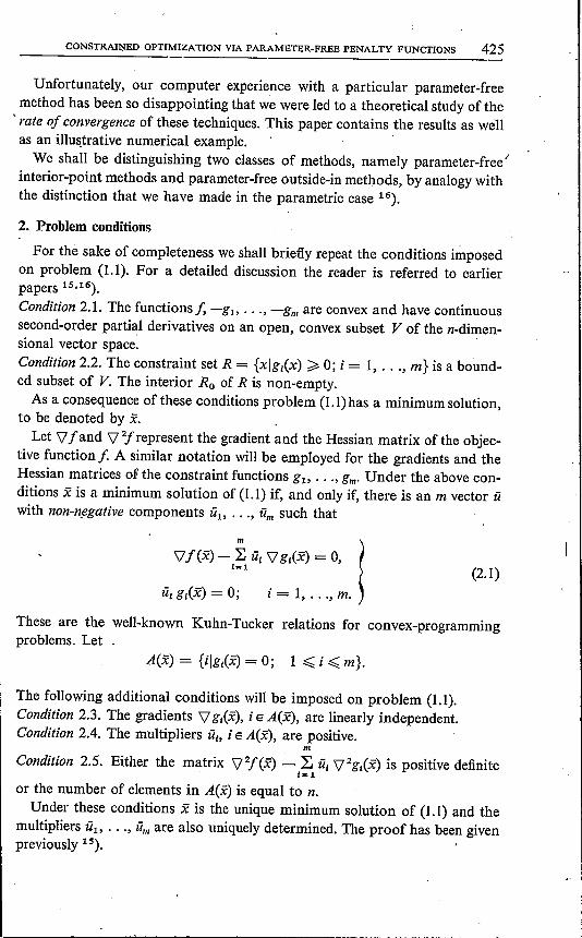
2. Problem conditions

For the sake of completeness we shall briefly repeat the conditions imposedon problem (1.1). For a detailed discussion the reader is referred to earlierpapers 15.16).

Condition 2.1. The functions/, -gl> ... , -gm are convex and have continuoussecond-order partial derivatives on an open, convex subset V of the z-dimen-sional vector space.Condition 2.2. The constraint set R = {xlgl(x) ~ 0; i = 1, ... , m} is a bound-ed subset of V. The interior Ro of R is non-empty.As a consequence of these conditions problem (U) has a minimum solution,

to be denoted by X.Let \j f and \j2f represent the gradient and the Hessian matrix of the objec-

tive function f A similar notation will be employed for the gradients and theHessian matrices of the constraint functions g l' ... , gm' Under the above con-ditions X is a minimum solution of (U) if, and only if, there is an m vector û

with non-negative components Ü1, ••• , üm such that

17f(X)-,~ u, 17g,(X) ~ 0, lülgl(x) = 0; 1- 1, ... , m.

(2.1)

These are the well-known Kuhn-Tucker relations for convex-programmingproblems. Let

A(x) = {ilgl(x) = 0; 1:::;; i :::;;m}.

The following additional conditions will be imposed on problem (1.1).Condition 2.3. The gradients \] gl(X), iE A(x), are linearly independent.Condition 2.4. The multipliers Üh i E A(x), are positive.

m

Condition 2.5. Either the matrix \j2f(x) - ~ ÜI \j2gl(X) is positive definite1=1

or the number of elements in A(x) is equal to n.Under these conditions X is the unique minimum solution of (1.1) and the

multipliers û., ... , iirn are also uniquely determined. The proof has been givenpreviously 15).

426 F. A. LOOTSMA

In what follows it will be convenient to think of the constraints as arrangedin such a way that A(x) = {I, ... , ct}. Then

g,(x) = 0;g,(x) > 0;

o, > 0;û, = 0;

i= 1, ... , ct, }i= ct + 1, ... , m.

(2.2)

3. Parameter-free interior-point methods

A sequence {X(k)} of points converging to x is generated in the following. way. The algorithm starts from an arbitrary x(O) in the interior Ro of R. Sup-pose that X(k-l) E Ro has already been computed. Let

fk-l =/ [X(k-l)]

andDk-1 = {xl/(x) <fk-l' xERO}' (3.1)

The parameter-free penalty function to be considered in the kth step has the, form

III

-cp [fk-l - f(x)] - ~ cp [g,(x)].'=1

(3.2)

Here, cp is a function of one variable, y say, satisfying the conditions listedbelow. These conditions were also imposed in the parametrie case 16) so thatlater on the relationship with parametrie methods can easily be demonstrated.Condition 3.1. The function cp(y) is concave and analytic for every y > O.Condition 3.2. lts derivative cp'(y) is positive for every y > 0 and has a poleof order A at y = O.It can readily be seen that cp is monotonically increasing in the interval

(0, (0); furthermore, it has a logarithmic singularity or, if A> 1, a pole oforder A-I at y = O. Hence

lim cp(y) = -00.yj,o

,Condition 3.1 implies the convexity of the penalty function (3.2) over Dk-1•

Now, let X(k) be a point minimizing (3.2) over Dk-1• The proof that such apoint exists will be omitted here since it can readily be derived after a slightmodification of the existence theorem given by Fiacco and McCormick ~) forthe particular case that cp(y) = _y-l. In order to ensure the uniqueness of X(k)

we shall be assuming that "(3.2) is strictly convex over Dk-1•

An interesting example of a parameter-free penalty function is obtained bysubstituting cp(y) = In y into (3.2). A minimizing point X(k) can then also befound by the maximizing over Dk-1 of

III

[fk-l - f(x)] TI g,(x),1=1

(3.3)

CONSTRAINED OPTIMIZATION VIA PARAMETER-FREE PENALTY FUNCTIONS 427

which is an example of the general distance function introduced by Huard 12).More generally, Huard has referred to X(k) as a centre of Dk-1. In what followswe shall be using the name "centre" for the points X(k) in the case where (3.2)is employed.It follows easily from the properties of Dk-1 that

fk-1 > fk ';::;f(x).

If x is an interior point of R, it may happen that X(k) coincides with x. Thenthe process terminates in a finite number of steps. We shall restrict our attentionhere to the case where x is a boundary point of R. Then we have

Generalization of a convergence theorem presented by Fiacco and McCor-mick 8) leads to

lim fk = f(x),k~ct)

(3.4)

and on the grounds of the conditions 2.3 to 2.5, implying the uniqueness of x,we can write

lim X(k) = x.k-+OJ

(3.5)

The gradient of (3.2) vanishes at X(k) since Dk-1 is an open set. Hence we haveIII

f[X(k)] - L cp'{g,[X(k)]} [X(k)]·= o.\J '{j, j, } \J s.cp k-1 - k

i= 1

(3.6)

Let us now consider a penalty function of the form

III

f(x) - r ~ cp[g,(x)],i= 1

(3.7)

which contains a controlling parameter r, and let x(r) denote a point minimizing(3.7) over the interior of R for a positive value of r. Such a point exists underconditions 2.1 and 2.2. The gradient of (3.7) vanishes at x(r), whence

m

\Jf[x(r)]-r ~ cp'{g,[x(r)]} \Jg,[x(r)] = O.i= 1

(3.8)

The formulas (3.6) and (3.8) reveal the close relationship between penalty-function techniques with and without controlling parameters. If we assume that(3.7) is strictly convex for any r> 0 so that x(r) is uniquely determined, andif we define

(3.9)we can immediately write

(3.10)

428 F. A. LOOTSMA

Apparently? a parameter-free interior-point method generates a sequence {X(k)}

of points on the curve {x(/')Ir > O} originating from a corresponding para-metric method or, and this is a particularly pleasant feature, a parameter-freemethod is a parametrie method adjusting the controlling parameter automati-cally. The adjusted parameter value which is given by (3.9) will here be termedthe equivalent I' value: it embeds the centre X(k) in the curve {x(r)Ir > O}.

The sequence {I'd is a mono tonic, decreasing null sequence. In order toshow this, let us start by defining

i= 1, ... , m. (3.11)

m

From (3.10) and the property that xC/') minimizes (3.7) we can infer

Ik-rk (IJk<1k+1-rk (lJk+1,1k+1 - rk+l (lJk+1<Ik - rk+1 (IJk,

whence(/'k+! - rk) Uk - Ik+ 1) < O.

Then /'k+1 < r, since Ik >Ik+ L' Finally, (3.4) and (3.9) lead to

lim /'k = O.k"''''

Lastly, we note that a feasible solution of the dual problem of (1.1) can readilybe obtained if we define

The dual problem and the dual convergence of parametrie methods have alreadybeen discussed 16) so that we shall only recall here the limiting behaviour of(3.11) which is given by

lim u!(rk) = ü!;k ... co

i= 1, ... ,m. (3.12)

4. Parameter-free outside-in methods

The development of parameter-free versions can readily be extended to theclass of outside-in methods by analogy with the mode of operation in the preced-ing section. First of all, however, we may note that in this section the set- Vnamed in conditions 2.1 and 2.2 is assumed to be the n-dimensional vectorspace En.

Generation of a sequence {.i(k)} of "centres" converging to x proceeds asfollows. We start with a lower estimate Ilo of I (x) such that

Ilo </(x). (4.1)

Let X(I) denote a point minimizing the parameter-free penalty function

-1jJ[,uo - I (X)] - ~ 1jJ[gt(X)],1=1

(4.2)

CONSTRAINED OPTIMIZATION VIA PARAMETER-FREE PENALTY FUNCTIONS 429

m

where 1jJ is a function of one variable y satisfying the following conditions.Condition 4.1. The function 1jJ(y) is concave for every y and 1jJ(y) -:- 0 forevery y ~ O. There is a function w(y) and a positive 8 such that w(y) is analyticfor all y < 8 and w(y) = 1jJ(y) for all y ~ O.Condition 4.2. The derivative w'(Y) of w(y) is positive for y < 0 and has azero of order ,u at y = O.

Condition 4.1 implies that (4.2) is convex on En. In what follows we shallbe assuming that (4.2) is strictly convex so that the minimizing point X(l) isuniquely determined.An example of a penalty function of the type (4.2) is obtained by the sub-

stitution of1jJ(y) = =min? (0, y) (4.3)

so that (4.2) reduces tom

min" [0, ,uo - I (x)] + ~ min? [0, gt(x)].1= 1

The function (4.3) is the function that we have been using for computationalpurposes. Its corresponding w function reads w(y) = _y2, the derivative ofwhich has a zero of order 1 at y = O.If the minimum solution x of (1.1) happens to be a point minimizing the

objective function lover Em then x(1) = x, and the process terminates afterone step. In the discussion to follow it is therefore assumed that x does notminimize lover En. This implies that x is a boundary point of R. It can thenreadily be shown that

,uo <f[x(1)] </(x).

For the rest we may proceed along the same lines as in sec. 3 so that a detailedexposition can be omitted. Let

Ik-l = f[X(k-l)]

and let X(k) denote the point minimizingm

(4.4)

over En. Then we have

Moreover,lim X(k) = x.k->'"

(4.5)

430 F. A. LOOTSMA

The gradient of (4.4) vanishes at X(k). One can then easily show that X(k) isthe point minimizing the parametrie penalty function

1 mI(x) - - I:1jJ[gl(x)]

S 1=1(4.6)

for S equal to( 4.7)

As before, we shall refer to X(k) as a "centre" and to Sk as the equivalent S valueembedding the centre X(k) in the curve {x(S)Is > O} of points that minimize(4.6). The sequence {Sk} is a monotonie, decreasing null sequence. Lastly, wedefine

i= 1, ... ,m, (4.8)

and we havelim UI(Sk) = ÜI;k-a)

i= 1, ... ,m. (4.9)

S. Rate of convergence

Our computational experience with the parameter-free method based on (4.3)and (4.4) has been so disappointing that we were forced to a more profoundinvestigation of the rate of convergence. In this section we shall be dealing with

I'lim _k_ (5.1)k->a) I'k-1

andSk

(5.2)lim -_k->a) Sk-1

i= 1, ... , m. (5.3)

for the parameter-free interior-point and outside-in methods respectively. Thereare obvious reasons for adopting (5.1) and (5.2) as a "measure ofeffectiveness".These quantities yield the ultimate rate of convergence of the procedure andfor a variety of problems the limiting value appears to be approximated rathersoon. If the problem functions f, g 1, •.. , gm are linear, the ratio Sk/Sk-l is evenindependent of k. Furthermore, (5.1) and (5.2) are decisive for the success ofextrapolation devices as shown by Bulirsch and Stoer 1.2) and Laurent 13).

Let us start with formula (5.2). On the basis of (4.7) and (4.8) we can write

It follows from (2.2), (4.5), (4.9) and from the conditions 4.1 and 4.2 that anumber K exists such that for all k > K we have

gl[X(k)] < 0;gl[X(k)] > 0;

UI(Sk) > 0;U1(Sk) = 0;

i = 1, ... , oe,i = oe + 1, ... , m.

CONSTRAINED OPTIMIZATION VIA PARAMETER-FREE PENALTY FUNCTIONS 431

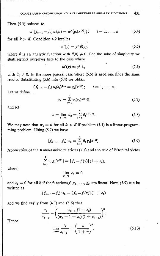
Then (5.3) reduces to

a>'[fk-i -Ik] Ut(Sk) = cv' {gt[X(k)]};

for all k > K. Condition 4.2 implies

i = 1, ... , IX (5.4)

cv'(y) = y" O(y), (5.5)

where 0 is an analytic function with 0(0) =1= O. For the sake of simplicity weshall restrict ourselves here to the case where

cv'(y) = y" 00 (5.6)

with 00 =1= O. In the more general case where (5.5) is used one finds the sameresults. Substituting (5.6) into (5.4) we obtain

i = 1, ... , IX.

Let us define"

(5.7)

and let"Hi = lim Wk = ~ Ü/+i/Il•

k-HIJ 1= 1(5.8)

We may note that Wk = Hi for all k > K if problem (1.1) is a linear-program-ming problem. Using (5.7) we have

a

(5.9)

Application ofthe Kuhn-Tucker relations (2.1) and the rule ofI'Höpital yields

"

where

and Bk = 0 for all k if the functions/, gl> ... , gm are linear. Now, (5.9) can bewritten as

and we find easily from (4.7) and (5.6) that

Sk ( Wk-i (1 + Bk) )"Sk-i = (Wk + 1+ Bk) (1 + Bk-i) .

Hence. Sk (Hi)"hm--= --- .k...ooSk_i 1+ W

(5.10)

432 F. A. LOOTSMA

In the case where ft = 1 (if, for example, (4.3) and (4.4) are used) we have

• Sk . IlülJ2hm--= ,k-+<1J Sk-1 1+ IIüW (5.11)

whereex

IIüW = ~ ü?1=1

It will immediately be clear that the convergence of the procedure can be accel-erated considerably if the objective function is given a smaller weight. Let usreplace (1.1) by the' problem

minimize pf(x) su~ject ~o_ } .gl(x) ~ 0, l - 1, ... , m,

(5.12)

where p denotes a positive number. Let u* denote the m vector of multipliersassociated with the minimum solution x of (5.12). Then u* = p û, so that(5..11) reduces to

Sk p211üWlim -- = -----k~aJ Sk-1 1+ p2 IIüW

A similar result can be obtained for the more general formula (5.10).. This acceleration can be made plausible from inspection of the penalty func-tion (4.4). Any point minimizing the second term

(5.13)

111

will be feasible. It is the first term in (4.4) which causes unfeasibility ofthe nextcentre X(k). A smaller weight of the objective function will apparently decreasethe weight of the first term. In so doing, it improves the rate of convergence.

Let us now turn to the interior-point methods. For (5.1) we find in a similarway

r (-).iI.1. k Vlm --= --k~aJrk_1 l+v' (5.14)

whereexv = ~ Üt1-1/).

1=1

If À -:- 1, we have the method of centres presented by Huard 12). The penaltyfunction is then given by (3.3), and formula (5.14) reduces to

rk Cl(

lim --=--,k~aJ rk-1 Cl( + 1

where o: stands for the number of active constraints at the minimum solution x.

(5.15)

CONSTRAINED OPTIMIZATION VIA PARAMETER-FREE PENALTY FUNCTIONS 433

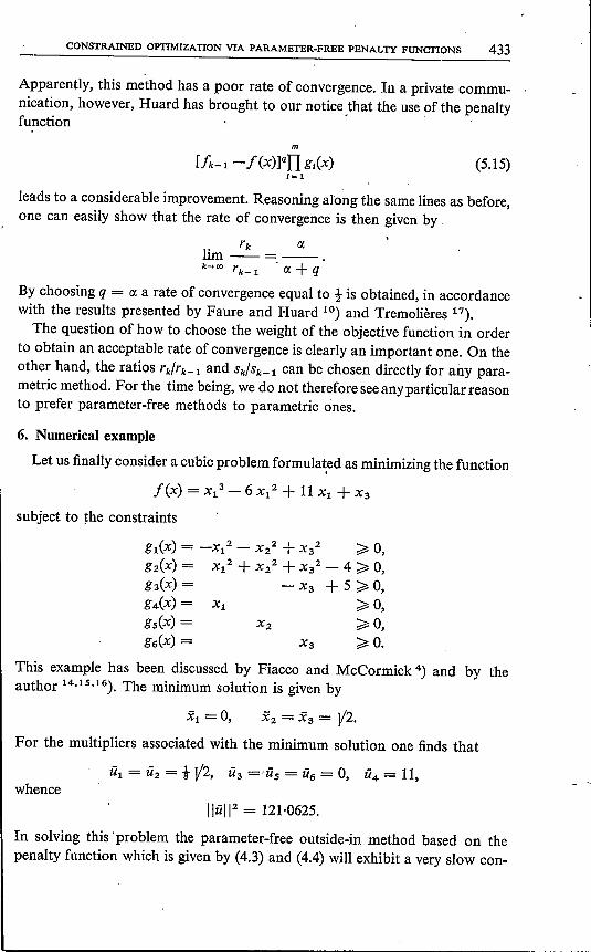
Apparently, this method has a poor rate of convergence. In a private commu-nication, however, Huard has brought to our notice ,that the use of the penaltyfunction

m

1=1

leads to a considerable improvement. Reasoning along the same lines as before,one can easily show that the rate of convergence is then given by .

rk ()(lim --. =--.k->c" rk-1 '()( + q

By choosing q = ()(a rate of convergence equal to t is obtained, in accordancewith the results presented by Faure and Huard 10) and Tremolières 17).The question of how to choose the weight of the objective function in order

to obtain an acceptable rate of convergence is clearly an important one. On theother hand, the ratios rk/rk-1 and Sk/Sk_1 can be chosen directly for any para-metric method. For the time being, we do not therefore see any particular reasonto prefer parameter-free methods to parametrie ones.

6. Numerical example

Let us finally consider a cubic problem formulated as minimizing the function

f(x) = X13 - 6 X12 + 11 Xl + X3

subject to the constraints

gl(X) = -X12 - X22 + X32 ~ 0,g2(X) = X12 + X22 + X32 - 4 ~ 0,g3(X) = - X3 + 5 ~ 0,g4(X) = Xl ~ 0,gs(X) = X2 ~ 0,g6(X) = X3 ~ 0.

This example has been discussed by Fiacco and McCormick 4) and by theauthor 14.1S.16). The minimum solution is given by

For the multipliers associated with the minimum solution one finds that

Ül = Ü2 = t V2, Ü3 ='üs = Ü6 = 0, Ü4 = 11,whence

IlüW = 121·0625.

, In solving this 'problem the parameter-free outside-in method based on thepenalty function which is given by (4.3) 'and (4.4) will exhibit a very slow con-

434 F. A. LOOTSMA

vergence. It is clear from (5.11) that

Sk >

lim -- = 0·9918.k-+oo Sk-l

Table I shows computer results for the above-named method applied to thecubic problem. Column 2 gives the computed objective-function values in the"centres" X(k); the entry in row 0 is the lower estimate /ho discussed in sec. 4.The equivalent S values can easily be calculated from these function valuessince (4.3) and (4.7) yield

~ Sk = 2 Uk - fk'-1)'

Let us now attach a weight p = 0·1 to the objective function. Then formula(5.13) leads to

Sk 'lim -- = 0·5476.k-+oo Sk-1

The corresponding computer results for this case, where to f(x) is minimized,are displayed in table 11.

TABLE I

Computer solution of cubic example with a parameter-free outside-in method

1 2 3 4

k fk Sk Sk/Sk-1

0 0 - -1 0,958980.10- 2 0.19180.10-1 -2 0.191258.10-1 0.19072.10-1 0·99443 0.286082.10-1 0.18965.10-1 0·99444 0.380371.10-1 0.18858.10-1 0·99445 0'474126.10-1 0.18751.10-1 0·9943

6 0.567351.10-1 0.18645.10-1 0·9943

7 0.660047.10-1 0.18539.10-1 0·9943

8 0'752215.10-1 0.18434.10-1 0·99439 0.843858.10-1 0.18329.10-1 . 0·994310 0'934976.10-1 0.18224.10-1 0·9943

11 0·102557 , 0.18119.10-1 0·994212 0·111565 0.18015.10-1 0·994313 0·120521 0'17911.10-1 0·994214 0·129425 0.17808.10-1 0·9942

15 0·138277 0.17705.10-1 0·9942

CONSTRAINED OPTIMIZATION VIA ,PARAMETER-FREE PENALTY FUNCTIONS 435

TABLE II

Computer solution of cubic example with a parameter-free outside-in method.The objective function is given the weight p = 0'1

1 2 3 4

k Ik Sk Sk/Sk-l

0 0 - -1 0'599855.10-1 0·11997 -2 0.954944.10-1 0.71018.10-1 0·59203 0'115846 0.40703.10-1 0·57314 0·127284 0.22875.10-1 0·56205 0·133639 0.12710.10-1 0·55566 0·137147 0.70167.10-2 0·55217 0·139082 0.38703.10-2 0·55168 0·140142 0.21202.10-2 0·54789 0·140723 0.11609.10-2 0·547510 0'141040 0.63387.10-3 0·546011 0·141213 0.34601.10-3 0·545912 0·141307 0.18879.10-3 0·545613 0·141359 0.10360.10-3 0·548814 0·141387 0.56562.10-4 0·546015 0·141403 0.30959.10-4 0·5473

The basis for extrapolation in the parametrie case can equally be used forthe parameter-free versions since the centres are situated on the trajectory ofpoints that minimize a parametrie penalty function. We have applied an extra-polation procedure in order to accelerate the process of solving the cubicexample in the case where the objective function was given the weight p = O·l.The results are displayed in table Ill. Minimization of the penalty function wascarried out in accordance with the algorithm of Davidon 3) as described byFletcher and Powell+'}, Column 7 lists the number of iterations required inorder to minimize the penalty function with the preceding centre as startingpoint. Column 3 gives the equivalent S values. The .word "extrapolation" inthe first column announces the results dbtained by extrapolation on the pre-ceding centres. The extrapolation procedure is based on the series expansion

which has been derived previously 16).

,

436 F. A. LOOTSMA

-

TABLE III

Computer solution of cubic example with a parameter-free outside-in methodand an extrapolation procedure. The objective function is given the weightp = 0·1

1 2 3 4 5 6 7

k I ik Sk x/k) xik) X3(k) iterations

0 0 - - - - -1 0.599855.10-1 0·11997 -0.712005.10-1 1·41242 1·41384 72 0.954944.10-1 0.71018.10-1 -0.408167.10-1 1-41362 1·41399 7

extrapolation 0·145003 - 0.326173.10- 2 1·41537 1·41421 -3 0·115846 0.40703.10-1 -0.229504.10 - 1 1·41403 1·41409 7

extrapolation 0·141308 - -0.103131.10- 3 1·41416 1·41421 -4 0·127284 0.22875.10-1 -0.127571.10-1 1·41416 1·41414 6

extrapolation 0·141424 - 0.200922.10 - 5 1·41422 1·41421 -5 0·133639 0.12710.10-1 -0.704444.10-2 1·41420 1·41417 6

f extrapolation 0·141421 - -0.211812.10-7 1·41421 1·41421 -

TABLEIV,

Computer solution of cubic example with a parametrie outside-in methodand an extrapolation procedure.

1 2 3 4 5 6 7

k f[x(sk)l Sk Xl(S,J X2(Sk) X3(Sk) iterations

1 0·748902 0.100.10-1 -0.585654.10-1 1·41300 1·41390 82 1·09729 0.500.10-2 -0.283567.10-1 1·41393 1·41406 7

extrapolation 1·43456 - 0.185188.10- 2 1·41486 1·41421 -3 1·25940 0.250.10-2 -0.139601.10-1 1·41414 1·41414 7

extrapolation 1·41383 - -0.353188.10-4 1·41419 1·41421 -4 1·33769 0.125.10-2 -0.692704.10- 2 1·41420 1-41417 6

extrapolation 1·41422 - 0.367326.10-6 1·41421 1·41421 -5 1·37617 0.625.10-3 -0.345045.10-2 1-41421 1·41419 6

extrapolation 1·41421 - -0.789921.10-8 1·41421 1·41421 -

Finally, table IV gives the results of the corresponding parametrie methodworking with the penalty function

Eindhoven, October 1968

which is obtained by substituting (4.3) into (4.6). Column 3 shows here thesuccessive values Sk which are a priori assigned to the controlling parameter s.In comparing tables III and IV one should remember the different weights ofthe objective function.

CONSTRAINED OPTIMIZATION VIA PARAMETER-FREE PENALTY FUNCTIONS 437

REFERENCES1) R. Bulirsch, Num. Math. 6, 6-16, 1964.2) R. Bulirsch and J. Stoer, Num. Math. 6, 413-427, 1964.3) W. C. Davidon, Variable metric method for minimization, AEC Research and Develop-

ment report, ANL-5990, 1959.4) A. V. Fiacco and G. P. McCormick, Programming under nonlinear constraints by

unconstrained minimization: a primal-dual method, Research Analysis Corporation,RAC-TP-96, 1963.

5) A. V. Fiacco and G. P. McCormick, Management Science 10, 360-366, 1964.6) A. V. Fiacco and G. P. McCormick, Management Science 12, 816-828, 1966.7) A. V. Fiacco and G. P. McCormick, SIAM J. appl. Math. 15, 505-515, 1967.8) A. V. Fiacco and G. P. McCormick, Operations Research 15,820-827, 1967.9) A. V. Fiacco, Sequential unconstrained minimization methods for nonlinear program-

ming, Thesis, Northwestern University, Evanston, Illinois, 1967. .10) P. Faure and P. Huard, Résultats nouveaux relatifs à la méthode des centres. Paper

presented at the fourth international conference on Operations Research, Boston, 1966.11) R. Fletcher and M. J. D. Powell, The Computer Journal 6, 163-168, 1963.12) P. Huard in J. Abadie (ed.), Nonlinear programming, North-Holland Pub), Co.,

Amsterdam, 1967, pp. 209-219.13) P. J. Laurent, C.R. Acad. Sci. Paris 256, 1435-1437, 1963.14) F. A. Lootsma, Philips Res. Repts 22, 329-344, 1967.15) F. A. Lootsma, Philips Res. Repts 23,108-117, 1968.16) F. A. Lootsma, Philips Res. Repts 23,408-423, 1968.17) R. Tremolières, La méthode des centres à troncature variable, Thèse, Paris, 1968.18) W. I. Zangwi1l, Management Science 13, 344-358, 1967.