RD-fi44 035 PARAMETER ESTIMATION IN A CONSTRAINED STATE SPACE(U) i/iI NAVAL UNDERWATER SYSTEMS CENTER NEWPORT RII K F GONG ET AL. 28 JUN 84 NUSC-6286

UNCLASSIFIED F/ 12/ NL

1.5

11111 11.2_

11111 1.5 11111J6

MICROCOPY RESOLUTION TEST CHARTNATIONAL BUREAU OF STANDARDS- 1963-A

NUSC Reprint Report 62628 June 1934

Parameter Estimation in aConstrained State Space

Kai F. GongAntonio A. MagliaroSteven C. Nardone

Combat Control Systems Department

U')In

a DTIC

.4 A

- Naval Underwater Systems CenterC Newport, Rhode Island I New London, Connecticut.. LJ

: I Approv I for public release; distribution unlimited.

Rep. i f an article published In the IEEE 1963 Conferencem Ilec ird 4f the Seventeenth Asilomer Conference on Circuits,

1 Systems and Computers.

84t 08 06 057

IAccession ForNTIS GIRA&IDTIC TABU:iannounoed ["Justificatlo7

By___________

PARAMETER ESTIMATION IN A CONSTRAINED STATE SPACE IDistribution/

Availability Codes

Kai y. Gong . Avail and/orAntonio A. asliaro Dit special

Steven C. Nardoee

4 U.S. Naval Underwater System centerNewport. Rhode Island 02841

When the source is know. to be confined to aThis paper examines the problems of state simply-connected region, it is possible to

estiation for a moving acoustic source confined to capitalize on such Information via multiple-

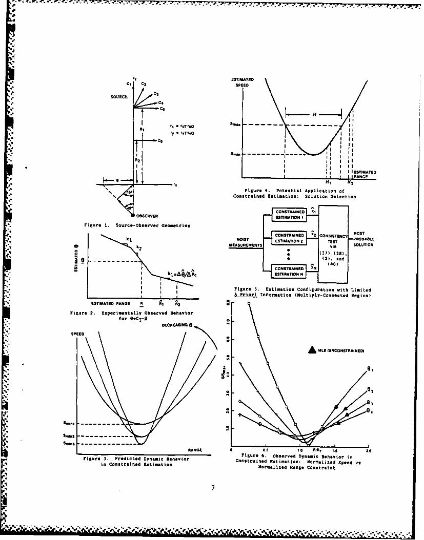
a well-defined. simply-connected or multiply- parameter constrained estimation. This is realizedconnected region of state space. A multiple- through augmentation of the Information mtriz byparameter constrained estimator that provides satisfying the Kuhn-Tucker conditions 3 or byenhanced performance and that permits determina- treating the constraints as pseudo-measurements.tion of the moet probable solution is presented. Convergence is guaranteed by adaptively adjustingThe estinmator is a batch processor that yields both the weights of the constrained parameters.dynamic &ad residual classifiers, the behavior ofwhich is shown to be dependent on source-observer When the source is known only to be confined ingeometry. The proposed realization is well-suited one of several possible well-defined finitefor solution selection through hypothesis testing. regions, a parallel configuration with multipleExperimental results showing estimator performance constraints is presented. The configurationare presented and solution quality is discussed, utilizes both dynamic and residual clues to

1 classify the solution as to its most probable state1. INTRODUCTION space. The dynamic clue or classifier is defined

in terms of a measure of deviation of the estimatedIn the underwater environment there are velocity parameters from its expected range of

numerous situations In which a source is known to values. Residuals are exploited by determinationbe confined to one of several, well-defined regions of expected variance and whiteness measures.of the state space. Effective state estimationunder these conditions requires that smaxinum use be Under the above Implementation, the ability tomade of all available information, and that some provide the most probable estimate of the state, ormeasure of solution quality be provided. Speci- solution enhancement and a measure of solutionfically, constraints on the state space environment quality, is dependent upon the amount of a prioriare critical for problems characterized by large information available. Experimental results

% range-to-baseline ratios or high levels of demonstrating system performance for various casesmeasurement noise. Previous work has demonstrated outlined above are presented.that for the case where only bearing measurementsinvolving high levels of "effective noise" are I. UNCONSTRAINED ESTIMATIONavailable, a phenomenon is experienced wherebysignificant deterioration in performance occurs The problem under consideration involves thewith increasing range or noise level.1.2 That estimation of the position and velocity of a con-study also examined estimation under a speed con- stant velocity acoustic source from noise-corruptedstraint and demonstrated significant improvement measurements. The source-observer scenario is illus-

" when such & orion information was included. Often, trated in figure 1. Let (raT, ryT) and (r1o, ryO )additional known parameters or knowledge of the be the positional components of the source and

" physical constraints on some function of the source receiver, respectively. The discretized version ofstate components (such as a bound on range, speed, the dynamic process is given in Table 1. For theor depth) are available and should be ezploited. bearings-only case. the measurement is given by

This paper addresses the problem of estimating z(k)-(k)the state and providing a measure of the quality ofthe solution for a source confined to a well- tan-- , (1)defined region of the state space. A multiple-parweter constrained estimator is presented for which represents a nonlinear model relating the(1) enhancing the quality of estimates when & priori noise-free measurements to the unknown sourceinformation constrains the state to a known (simply- state. In (T-6). 'T is the estimated state atconnected) region, and (2) determining the most the selected reference time. its value at anyprobable solution when the regions are distinct other timeis determined via (T-l) and used in (1)(multiply-connected). to produce the appropriate bearing angle.

Y17

% When the number of measurements, K, Is greater Equation (11) represents the solution for thethan 4, (T-6) represents an overdetermined sys5tem unconstrained maximum likelihood estimator.of nonlinear equations. A weighted least-squares performance of the entimtor has been assessed byapproach minimizes the norm of the residual vector examination of the ideal Information matrix, or

Crame~r-1ao bound, for large range-to-basetline-1a (Z _Z(1 )1 (2) seometie.1 In this situation, the assumptioms

T ~Of conStant range and sy menetric geomfetry are

wbere S.D06gook). al Is the bearing measurmnt valid. Under these conditions. the elgenvalues ofnoise standard deviation, and ZVIT) is the bearing the ideal information matriz are given in theseunegnrtdb the estimated state, t Via second colum of Table 2.1 Note that significantsequenc ge4) ntd by.Th rblmi cmlted dettioratiun in performance occurs with increasing

*by the unusual observability properties of this ranget or noise level.

system, 4 especially for long range scenarios.V tlU. CSIXRAT!0U-in COUSMhINED STATE SPACE

The inium f th nom-suare eror.Since errors is the estimates of range and range

T -2 rate are inversely proportional to Alto and Ai.3 S-Z'~ 'Z. _Z(Y1) *3 respectively, it is seem from Table 2 that

- variations in these estimates significantlyIs found when the estimate iTcauses the $radient increase for large values of "effective noise," rao/B.GWz.1 )-WJaz1 to vanish; i-.. where 3 denotes synthetic baseline. When unreason-

able estimates result, 1 priori information or

-,Ci)=(az(i 1 )iai I S1 (z.-ZCa)].(OI. (4) heuristic data can be utilized to advantage. Often.T T T Tknown parameters or knowledge of the physical con-

%For Gaussian noise. the resulting iT represents straints on san functions of the state components

the naximum likelihood estimator (HUl). The are available and should be exploited. Under thesepremltiplying matrix is given by conditions, the problem then becomes one of

minimizing the cost function

where T TT jmjTjS2ZjTj()

-l gi -1 k] -.l.. 6 subject to the constraint

f~iT)Sb . (13)

ComoI -mim 1I t 0Como I -t asin 1o Wee. thyT) and b denote the vectors I(f1,f2 . -M)

coso2 -sin 2 t 0Com 2 2t SiO 2and (Cb1 ,b2 .... ,b 11 ) IT. respectively, and N is the

A1x )W 05 2 -if t5 4 ts~ (t0,t1t) (7) number of constraints. Denoting fj-±A~jiHZ, theT necessary and sufficient couditions tot J to be mini-

mum Is given by the Kuhn-Tucker conditions.2'3 That Is,

coso K -$tnA Kt scosO K -at smin$ 1 K T-2-Tz .; +4 (A3 It S_ ij 1oN T'

and where to is the data sampling period and *(t 0 .t3 t) j+Iil i-Iis the transition matrix between the Initial time, to0and reference time, tit. The kth element of the ^T- -2 r P T T (1-diagonal matrix of (6), j J e-0 1 li

i(k)-((? CT k)-r C0() Y2.IT k)-r 0(k))I)2 I)l/Kb

is the estimated range at the kth instant, and P? 11.2. N. (14c)

*where *i,1ml,2_. N in a scalar to be determined.in (7) is the corresponding bearing estimate. Hence, F:tesnl aaee osritcs.0cnbone seeks to solve the nolineor set of equations sos te sie parnveneter consta itcaste, vicab

A (z T)a S ( Z-Z~iT)_0 (10) Pj+l-Pj+A6 (15

for 4y. Employing the Causs-Newton iterative where

methods to solve (10) yields

whereA and Z. are evaluated at ij. and the and where W is the state vector associated withstep size, &j. is selected at each iteration to fCiT), PW is its covariance, and d is selectedensure convergence, to ensure system stability. Multiple parameter

2

* *t* * * - N

constraints can be realized by either sequential or constrained parameter and then applying (14).

simultaneous processing via (14). For the case of Further comparison of (14) and (20) in regard to

single parameter constraint, experiments have shown their robustness, and analysis of the mechanisms

satisfactory convergence and stability for both that impact the estimate will be addressed inspeed and depth constraint

2.6. For the case of future studies.

speed constraint, an improvement factor of 2 in

localization error has been demonstrated. IV. CONSTRAINED ESTIMATION INSIMPLY-CONNECTED REGIONS

An alternative implementation of estimation ina constrained state space is to consider the When a Priori information constrains the source

constraints as "pseudo-measurements." If the to a known region (simply-connected), performancemeasurement vector is given by can be significantly improved. This can be demon-

" strated by examining the augmented information

Zp-(Zm,bJT+q , (17) matrix of (21) when range information, with

standard deviation, o, is available at K.

the cost function then becomes Jp=J+Jb where Under this condition,

Jbzh-f(2T)]Tp-2(b-f(2T1] (18) )Ti-2-2-l -T -2-

SR A ROR A (26)

subject to the constraints of (13). The solutionis obtained by finding an iT such that Jp is where

minimized. Setting the gradient aJp/3iT equal 0 0 0 0to zero and employing the Gauss-Newton iterative A"to.t E) (27)

0 ~- 0 0 0O O

T--2 -2i -14--I-2ZI.S+6.((A.R. S Ai A.R S Z cos K

Assuming uniform signal-to-noise ratio, the augmented

T 2T -2 b M (19) information matrix at K/2 becomes

K/2 k (k-K/?Qk J R (K/2 )Q

or IT-a 1!- 2.2k2](8+1 I. .z..1(Q.Q J Q .QJ .- -20- _l/2 -k-K12)Qk (k-K/2) 2 (K/2)12 (K/2)2 Q (2R

where Q is the modified infcrmation matrix given by where 1 [r co -sin

Abip bi ( k r 0 ssikcosk (29)

and k sin k kand

Abzaf(iT)/axT (22) 1[ i2A si na KCos t

Q-Dia TT k,Pi], (23) a R [sincosi Cos 2a K (30)

I TT K KZpe .(Z [b-f(xT) H )

T. (24) Using the assumption of symmetric geometry, 0(K/2) is

and where pi>O and is either known or can be diagonallzed;1

that Is,

determined adaptively via r cos 2 k 0 22

2? ~2 , (25) Ela~ 2 1 2r k 1 (31)ijOi L 0 sink

, until the constraints are satisfied. Experiments sadconducted utilizing (20) for the speed constraint s 2X 1have yielded equivalent results to those obtained ivia (14). Although the use of (14) for range Z(Q] si a 2 32

*4 constraint under adverse conditions has experienced 0 Cos2i R

some cases of slow rate of convergence, (20) has

provided stable and rapid solutions. Note, however, For long range scenarios, the range is assumed tothat (20) represents the solution of an unbiased be essentially constant; i.e., 3=rl. Under these

estimator; as such the modified information matrix conditions, the expected eigenvaluel of (K/?)

(or its inverse) must be interpreted appropriately are given in Table 2. The variance is given by the

consistent with the a oriogt data description. reciprocal of the eigenvalue, or

When insufficient description on the data-weighting

assignment is available, the modified information a 2()o2 (a)matris can be more appropriately generated by 2 u 33)

applying (i), or-in the case of slow convergence e 2 2 U R21iR 11 (33)

by utilizing the speed solution of (20) as the (3)+u (R)

'4. 3

% N,

where o2(p) is the variance of u due to the Thus, (37) and (38) provide the expected dynamic

parameter p alone. Clearly, if range information is behavior of source estimates. This is illustrated

given, the expected improvement factor in the reduc- in FIgure 3. The solution, dependent on the noise

tion of variance over bearings-only processing is conditions. may fall anywhere aLong the speed-range

[oa(2)Vo2(R)J/u2(R). Equation (33) can be curve. However, if the maxium speed, Sma, is

generalized when multiple parameters are known known a priori, the most probable solution musta priori and Q(K/2) is diagonalizable to yield then be bounded by Smax and Smin and. therefore,

is confined to R as shown in Figure 4. if. in2 addition, the source is known to be in either M,

2 u or R2 , knowledge of Smax then can eliminate

u I +2(0) 0-2(p) (34) R 2 as a possible solution.

Further insight can be gained by analyzing the

resulting in an improvement factor of effects of constraining the estimates away from the(l+o (3)£Io

2(p). Further analysis on the impact speed-range function. This corresponds to

of additional information is contained in reference . performing estimation with range and speedconstraints. Thus, given the estimate (STR),and if the parameters are constrained to

V. PROPERTIES OF ESTIMATION IN (ST,4.8), (35) then becomesCONSTRAINED STATE SPACE I

(RaR)(3.Al3).$TSin(0.a8)-Sosin(y n'r).

Based on the analysis in the previous section, (39)the availability of a priori information, heuristic where i=CO-O. Assuming small 46 and Ay. the result-or otherwise, can clearly provide improvement in ing bearing rate error, Ad, can be approximated assystem performance. However, in many situations.such as the one in which the source is known only &Am=(STIR)AC(-&C/2)coS*-(&oR./i R/i)E/(l+aR/R). (40)to be confined to one of several distinct regions(multiply-connected), only limited heuristic where AC is the change in d.T corresponding to at.information is available. Under these conditions,improvement in state estimation is still possible Equation (40) represents the slope of theby providing the most probable solution. residual, and can easily be computed for each leg

of constant observer velocity. Furthermore, itConsider the relation for cross-range-rate provides a measure of inconsistency and sensitivity

component in the state estimates. Such a measure can be usedin conjunction with the expected residual variance.

Ri.STsin(CT-0)-SOsin(Co-0) (Ii) as given by (3), to supply a more extensive descrip-tion of the residuals. To a certain estent. (3)

where b is the bearing rate, ST and SO are and (40) provide a "whiteness" measure. Thissource and observer speed, respectively, and CT measure can alternatively be obtained by performingand r) represent source and observer course, a spectral analysis on the residuals. Similarrespectively. Let (STCT. ,0) be the analysis can be performed for different constraintestimate obtained by constraining the range at combinations or with additional constraints.ic. The variation of speed as a function ofrange can be analyzed by perturbing (35) to yield Thus, when a priori information constrains the

source to one of several possible solution regions.A$1AR-( +RA'vARc)Is;O-[6R'[(ST+S)t (36) or when limited heuristic data are available, the

C C sin C TanG (36) estimation configuration of Figure 5 can be employed

where fieT-d and the assumption is made that along with (37), (38), (3), and (40) to provide the

AD/AOC=O. Generally. i(R) is point symmetrical about most probable solution.

(R,O) and can be approximatgd as piecewise linear VI. GENERAL OBSERVATIONS.(Figure 2). The quantity 0/AKC can be treated SOLUTION QUALTY. AND SELECTIONas a constant, k1 , within the interval (Rl,R 2 ).Therefore, the slope of the speed-range function can The analysis presented up to this point dealsbe rewritten as with the problem of estimating the state parameters

by capitalizing on any available a priori.... ..- - - information. Depending on geometry and amount of

CS/ARCT[(iC /AR C )-klSTcoseJ/(sin+aocos9). (M information (heuristic or otherwise), constrainedestimation can provide enhancement in the target

'clearly, 0 is geomtry and noise dependent and 15 state estimates either by reducing the state errorinversely related to the slope. As 6 increases, variances or by providing the most probablethe change in the speed estimate is less senstive solution(s). Some general observations areto range. The minimum speed can be computed about summarized as follows:(R,) by setting (37) to zero to yield

1. The speed-rnge relation of Figure 2 isSman2(ft+RA/A-C)/k~cos (38) derived by minimizing the cost function, J, and is

geometry dependent. The slope and minimum speedwhere k2 iS generally large for small 6. are predictable and can be analyzed via (37) andConsequently. geoe5tries with small • generally (38). For geometries that exhibit stronger across-have Smaller Smin. the-line-of-sight component, the magnitude of the

T. T '. 7 Z.7 T

J.

speed-rang. slope is smaller and the minimum speed cosO (see (37)). For the approximately symmetricis larger; furthermore, the residuals are more source-observer geometries considered, thesensitive to deviations from the solution curve. estimated course function is approximately point

symmetric about the point at KC(Smin(O)l where2. The availability of valid j priori aT,90*. In the case where 0 is near zero, the

information (e.g., range, speed, course) will 180* difference in the estimated course correspond-provide enhanced estimates with reduced state error ing to ranges on either side of RC($min(O)]variance, consistent with respect to both dynamic is reflected by a switch of sign for the slope ofand residual behaviors, the speed-range curve. As S increases, the last

term of (37) dominates; thus, the symmetric change3. The availability of valid speed or range of the estimated course about 90* in Figure 1 leads

information will enable the selection or to slopes for the speed-range plot which are equaldetermination of the mast probable solution based in magnitude but opposite in sign. This dynamicon dynamic and residual consistency tests, behavior is Illustrated in Figure 8 where a total

of 30 noise sequences have been applied.4. The dynamic behavior curve can potentially

be applied to determine the approximate dynamic Sensitivity of the state estimates is examinedbehavior of the process. by perturbing the range or speed estimate and by

monitoring the resulting residuals. The resultsS. In the absence of other information, the are shown in Figures 9 and 10. The shaded area of

physical constraint of maximum allowable speed and Figure 9 represents solutions which yield approxi-the predicted minimum speed can be employed to mately the same value of residual variance 'i.bound the solution heuristically. In addition, In essence, this area can be viewed as a region ofboth dynamic and residual clues can be employed to minimal d02; therefore, estimates located

% determine a solution region. outside the shaded region may yield residuals whichare statistically inconsistent and which should be

Based on the preceding observations, estimation rejected as possible solutions. This situation isvia the constrained approach provides improvements illustrated in Figure 10 when constraints werein system performance. Given a state estimate from imposed by utilizing an incompatible range-speedan algorithm, the dynamic and residual clues combination. In fact, the residuals have thecan provide a check on its validity. In addition, functional form etheto+A 0Tt-0e,. where Tt denotesthe constrained estimation approach provides the the length of the t

t leg, eto is the referenced

mechanisms that maximize the use of any available £ initial residual, and Pet is the random component.priori information. Furthermore, it can be employed For the noise free case, the slope Ait agrees well

for solution selection. with that given by (40). Thus, if incompatibleI oriro information Is employed, clues from the

Theoretically, the covariance matriz provides a residuals, such as ; and A t . can potentiallystatistical measure of solution quality assessment, be utilized to reject any invalid estimate. In thisalthough its validity is algorithm dependent. The context, both dynamic and residual clues can be ap-predictable dynamic and residuil behaviors and plied advantageously for solution quality assessment.solution bounds provided by constrained estimationclearly can be used as heuristic solution quality The improvement obtainable when good informationmeasures; and, when used in conjunction with the is utilized for constrained estimation iscovariance matrix, can provide a viable means for illustrated in Figure 11. In this figure, it cansolution quality assessment and solution selection, be seen that when the range, RCIOR, or speed

is given as heuristic data, the constrainedV[I. SINULATION RESULTS AND DISCUSSION estimator provides significant improvement in

solution accuracy and solution uncertaintyExperiments were conducted using the geometries reduction. Solution consistency is confirmed by

of Figure 1. A total of six geometries were both the dynamic behavior and the residuals.considered. A normalized observer speed (So/Sma)of 0.47 was employed. Source dynamics are given inTable 3. Zero mean Gaussian noise with 2* standard Estimation for the situation when the source is

deviation was added to the true bearing. A total known to be in one of three regions is demonstratedof 400 equispaced measurements were collected on in Figures 12 and 13. Information is alsoeach leg. All subsequent discussion is referenced available (with probability 1) in regard to theto the final time. source's maximum speed. The configuration of

Figure 5 is employed by constraining range to eachFigures 6 and 7 show the behavior of speed and respective region with and without the additional

course estimates as a function of the constrained speed constraint. For the case of constrainingrange for different OC T -3. The unconstrained MLE only range, hypothesis testing of maximum speed isestimates are also included for completeness. As employed, and the results show that the region.shown, the dynamic behavior is geometry dependent. denoted by I, is the true solution. For theAt the center portion of the course-range plot, the case of constraining both range and speed, themagnitude of the slope increases as the angle * residual clues of Figures 13a-c again provide thedecreases. Consequently, the geometry with the necessary information to select R, as the most

smallest * exhibits the smallest minimum speed, probable solution.as shown in Figure 6 (see (38)); also, the speed-range slope is muc i sharper with smaller Sgeometry since it varies inversely with sine and

.5

•7%17L

VIII. SUMMARY AND CONCLUSION Table 1. System Dynamics and Measurements

The problem of parameter estimation in a Source Statesconstrained state space that capitalizes on theutilizaton of g i information (or heuristic aT(k+l) - #(k+l.k)xT(k) (T-1)

*?'. data) was presented. A nonlinear estimator with s T(k) - r(k r W(k V (k) V (k)|Tmultiple constraints was considered and its T xT yT xT yT

properties analyzed. The estimator is a batch r i _processor that yields both dynamic and residualcharacteristics which permit solution enhancement, -

- * solution selection, and quality assessment. (T-3)Sensitivity of these characteristics is shown to Observer Statesdepend on source-observer geometry. Dynamic cluesz (k~l) - *(k+l~k)z Mt . A(k) (T-4)are common for low bearing rate trajectories, while o o

residual clues are most evident In scenarios having (where A(k) accounts for effects of maneuver)a noticeable across-the-line-of-slght velocity Tcomponent. While the ability to determine the $tate s0(Mk [r C0t) r (k)M V to(W V Y k)l (T-5)parameters via acoustic measurement processingbecomes increasingly difficult with deteriorating MaueetVcoconditions, effective utilization of a priori MaueetVcoinformation is shown to provide significant Z - ZI )+n (T-6)enchancement. Whe the source is known to be m T Tconfined in a well-defined region. enhancement is Z (T-7)realized by reducing the solution error variance. - n 2 CT-8)When the a Priori information or heuristic dataconstrain the source in one of several regions, the l = [0] (T-9)estimator is capable of providing the most probable T 2solution. In addition, both dynamic and residual kni,Diago . k 2z -. .K (T-lO)clues are predictable. These. when used inconjunction with the estimated state covariancematrix, can provide a viable measure of solutionquality. Table 2. ligenvalues of Q(K/2) via Processing Bearing

(with Range Constraint)

REFERENCES k X (D)+X (3), =• .N N N j j 1t II I- I. S.C. Nardone. A.G. Lindgren, and K.F. Gong, *A

Performance Analysis of Some Passive Bearings-only V () ( CR)Target Tracking Algorithms." 1 _____ NConference on Circuits, Systems and Computers. 3 2November 191. a, (K /12)(1/r a2 (K/2) 2 (0 2112)Cd(1 ,

2. K.F. Gong, S.C. Nardone. and A.G. Lindgren. 32 22 2 2"Passive Localization and Notion Analysis With a (II R3/144)(1/r 0 (K/2) (1l0RState Paremeter Constraint." 15th AailomarConference on circuits. Systems and Computers. 1 K/r 2ae (02 /12)(1/o)November 1981. 1

3. Maxwell Noton. Modern Control Ennineerin, a (K82/12)(1/r2,2

1/o

Pergamon Press, Inc., New York, 1972.Where Cu() is the elgenvalue of the P-component

4. S.C. Nardone and V.J. Aldala. "Observability due to (.); R1 and il are range and range-rateCriteria for Bearings-Only Target Notion Analysis." components perpendicular to the line of sight; andTERE Transactions on Aerospace and Electronic RI1 and R11 are range and range-rate componentsS"stems. Vol AES-17. No. 2. March 1981. Along the tine of sight.

S. G. Oahlquist and A. 8jork Itranslated by N. Table 3. Source Trajectory Parameters*'. Andersoni. Numerical Methods, Prentice Hall, 1974.Geom Course ei'CTiOi Normalized(Dot) (Dea) Speed/Range

6. K.F. Gong, S.E. Hammel. S.C. Nardons. and A Go 1 0 1.23Lindgren. "Utilization of Environmentally Perturbed 2 0Acoustic Measurements for Three-Dimensional Target 3 20 17.8 SS 1/ , 0.67Parameter Estimation.- 16th Ailomar Conference on 3 45 38.9 RlB - 9.5

Circuits. Systems and Computers, November 1982. 4 so ?0.17. S.C. Nardone, A.G. Lindgren, and K.r. Gong, 5 90 83.0 S/Smaz - O.47

"Measurements, Information, and Target Notion RI/B . 9.5Analysis." 17th Asilomar Conference o n Circuits, -9 .......... ........................ 0............Systems, and Comeuters, November 1983. 6 90 66.4 S a - 0.67

6*pR.''

- jN% % % i - *. ~ .

-- --

IV C ESTIMATEDC1 CI 2 SPEED

4, SOURCE

rx rxTrxo Sinax - -

1 ', : , ESTIMATEDs--- I I E

Ce,-I iii'

N 4s. Figure 4. Potential Application of- LS Constrained Estimation: Solution SelectionI%

OBSERVER

Figure 1. Source-Observer Geometries• . MOSTq CONSTRAINED X2CONSISTENCYt

*1 CNIY -ROAL

klNIYE, -ESTIMATION 2 TEST0 ®k2 MEASUREM NS VIA SOLUTION

li . •(3). and^ A .A CONSTRAINED X, (0

II a/,&Re ESTIMATION NU''UI I e/A-

Figure Estimation Configuration with Limited-"~ Pror iA A nformaton (Multiply-Connected Region)

A A0ESTIMATED RANGE R R1 R2

Figure 2. Experimentally Observed Behavior

for O8CT-0 ADECREASING6

* SPEED

AS MLE IUNCONSTRAINEDI

60 824%,"

IRANGE 0,S 1.0 1111111 1Is 2.0F ligure 6. Observed Dynamic Behavior inFiure 3. Predcted Dynamic Behavior Contrined Etiat(ion: N~or aLti ed Speed vs

in Constrained stimton Normalized Rne Consrat

Lab

- £ MLE (UIICOnstnId) MLE (UNCONSTRAINEDI

ccZ0

, 0,

0.5 1.0 1.5 2.0ARn

Figure 7. Observed Dynamic Behavior in ConstrainedEstimation: Course vs Normalized Range Constraint

0 001I.5 2.I

SFigure 9. Region of Minimal o

gE

, .~

_ IME (SECS)0 200 400 600 800

Figure 10. Bearing Residual vs Time;

=8e5, R/Rtrue=2.4, S/StL.ue l.0

0 .5 1.0 1.5 2.0

RI

Figure S. Normalized Speed vs Normalized Range

Constraint (O.0e) for 30 Noise Sequences

• ]Pd

X • TRUE• A - MLS (Unconstrained)

% 0- Sma CONSTRAINT0- RANGE CONSTRAINT%RANGE-SPEED CONSTRAINT

rn 7

E I TIM! ISECS)

0200 400 600 am0

Fig~ure 13&. Bearing Residual vs Time;9eGe, R/Rtruezl.0, S-St.ue<Sma

x

.0. 1.0 1. 2.0.. . . .. ; -

Figure 11. Solution Enhancement; via Utilizati on '/"-".,., .of Heuristic Information (e 1 ) - .

TIME (SECS)

",0200 400 600 00

Figure 13b. Bearing Residual vs Time;e-e6, R/Rtrue:2.3, S=Smax

0t

t - - -. - -- - .. .. .

o .0 urt no t ( .0 T .I. "

"T. TIME (SECS)

11110 200 400 600 800

Figurel 12. Solution Selection via Figure 13c. Bearing Residual vs Time;Contrained Estimatgion (e-e.) ee, RRtrue,3.4. S=S

02x

.. 44-

-'4

JrJ

Ts,

PAM,

4i4

.4,. 3, 3 4