CONSIDERATION OF SOLAR RADIATION IN FLARE DESIGN

A Thesis

by

ANKITA TANEJA

Submitted to the Office of Graduate and Professional Studies of

Texas A&M University

in partial fulfillment of the requirements for the degree of

MASTER OF SCIENCE

Chair of Committee, M. Sam Mannan

Committee Members, Mahmoud El-Halwagi

Sharath Girimaji

Head of Department, M. Nazmul Karim

May 2018

Major Subject: Chemical Engineering

Copyright 2018 Ankita Taneja

ii

ABSTRACT

At oil refineries and other chemical processing plants, a flare stack is used to get

rid of unwanted or excessive gases and relieve the system of excess pressure. These

gases can be generated during different stages of operation like startup or shutdown,

maintenance and process upsets. Since flares handle large amounts of toxic and

flammable materials, it makes the flaring operation hazardous. Combustion of huge

amount of gases releases heat which is radiated to the atmosphere. Heat radiated from

the flare makes it important for siting the flare at a proper location. The heat radiation

should not exceed recommended threshold levels so that people on-site and the

equipment are not affected. Thus, to have a well-designed flare, knowledge of total

radiation emitted from a flare is essential. It will aid in accurately estimating the flare

height and the area near the flare, which would sustain high levels of thermal radiation.

A common point of contention while calculating radiation level emitted from

flare is the decision of including solar radiation (SR) in the calculations. API 521

relegates this decision to the flare design company’s practices. Based on expert

judgement, some literature states that for all practical purposes, solar radiation

contribution can be discounted.

The work performed aims at presenting a framework which quantitatively

addresses aforementioned obscurity. The analysis helps flare designers to more

objectively decide whether to include SR in their analyses or treat it insignificant

contribution. The work studies the various factors that cause variation in SR value:

iii

location, time, and orientation of the surface. Considering all these parameters, an

appropriate value of SR is chosen as the solar contribution to the thermal radiation from

the flare. The effect of SR to the design of the flare is quantified by studying the change

in effect distance near the flare and the height of the flare. Consequence analysis

software PHAST is used to obtain these calculations. In addition, the outcome that SR

inclusion will have on the risk posed by the flare due to thermal radiation on personnel is

also examined. This is studied by measuring the change in lethality and heat stress

caused by radiation exposure.

iv

DEDICATION

To my mother Ranjana Taneja and my father Shanker Taneja for their

unconditional love and support in every decision I have taken. To my little sister Drishti

Taneja for bringing immense joy in my life.

v

ACKNOWLEDGEMENTS

I want to firstly thank my research advisor Dr. M. Sam Mannan for all his

support and feedback throughout my study. His dedication to the Mary Kay O’ Connor

Process Safety Center and process safety at large has continued to inspire me.

I would like to thank my committee members, Dr. Mahmoud El-Halwagi and Dr.

Sharath Girimaji for their guidance and support throughout the course of this research.

I want to appreciate the time devoted by Dr. Delphine Laboureur, Dr. Hans

Pasman and Dr. Bin Zhang in providing guidance for my research.

Thanks also go to my friends Kunal Das, Nikhil Mayadeo and Nilesh Ade for

being there in need and helping me in all ways they could.

I also thank the department faculty and staff for making my time at Texas A&M

University a great experience.

I am forever grateful to my mother, father and sister for showering their love and

being my life’s inspiration.

.

vi

CONTRIBUTORS AND FUNDING SOURCES

Contributors

This work was supported by a thesis committee consisting of Professor M. Sam

Mannan of the Department of Chemical Engineering, Professor Mahmoud-El Halwagi of

the Department of Chemical Engineering and Professor Sharath Girimaji of the

Department of Ocean Engineering.

The work conducted for this thesis was completed by the student independently.

Funding Sources

Graduate study was supported by Chemical Engineering Award from Department

of Chemical Engineering, Texas A&M University. TX Public Education Grant from the

state of Texas and Harry West Memorial Endowment from Mary Kay O’Connor Process

Safety Center at Texas A&M University was also awarded to support graduate study.

vii

TABLE OF CONTENTS

Page

ABSTRACT ....................................................................................................................... ii

DEDICATION .................................................................................................................. iv

ACKNOWLEDGEMENTS ............................................................................................... v

CONTRIBUTORS AND FUNDING SOURCES ............................................................. vi

TABLE OF CONTENTS ................................................................................................. vii

LIST OF FIGURES ........................................................................................................... ix

LIST OF TABLES ............................................................................................................ xi

1 INTRODUCTION ...................................................................................................... 1

2 LITERATURE REVIEW ........................................................................................... 4

3 STUDY OBJECTIVES ............................................................................................ 11

4 METHODOLOGY ................................................................................................... 13

4.1 Solar Radiation Calculation ............................................................................. 13 4.1.1 Earth-Sun Geometry ..................................................................................... 14

4.1.2 Solar Radiation Model.................................................................................. 17 4.1.3 Calculation Of Radiation For Different Orientation Of Surface .................. 21

4.2 Thermal Radiation From Flare ......................................................................... 24

4.3 Effect Of Solar Radiation Addition .................................................................. 28 4.3.1 Effect Distance From The Flare Base .......................................................... 28

4.3.2 Height Of Flare Stack And Corresponding Cost .......................................... 28 4.3.3 Probability Of Injury/Fatality ....................................................................... 29

5 RESULTS AND DISCUSSION .............................................................................. 32

5.1 Solar Radiation ................................................................................................. 32 5.1.1 Solar Radiation With Different Orientation Of A Vertical Surface ............. 32 5.1.2 Maximum Solar Radiation ........................................................................... 36

5.2 Total Thermal Radiation .................................................................................. 39

5.2.1 Intensity Radii And Effect Zone .................................................................. 39 5.2.2 Flare Height .................................................................................................. 42

viii

5.2.3 Risk Assessment ........................................................................................... 43

6 CONCLUSIONS AND RECOMMENDATIONS ................................................... 53

REFERENCES ................................................................................................................. 56

APPENDIX ...................................................................................................................... 60

ix

LIST OF FIGURES

Page

Figure 1. Solar altitude angle β, and solar azimuth angle, φ ............................................ 16

Figure 2. Depiction of direct and diffuse solar radiation ................................................. 19

Figure 3. Variation of τb with day number, n ................................................................... 20

Figure 4. Variation of τd with day number, n ................................................................... 20

Figure 5. Tilt angle and azimuth angle for a vertical surface ........................................... 21

Figure 6. Different values of surface azimuth angle ψ considered for a vertical

surface ............................................................................................................... 24

Figure 7. Solar radiation on a vertical surface facing South vs. time for different days

of the year ......................................................................................................... 33

Figure 8. Solar radiation on a vertical surface facing North vs. time for different days

of the year ......................................................................................................... 34

Figure 9. Solar radiation on a vertical surface facing East vs. time for different days

of the year ......................................................................................................... 34

Figure 10. Solar radiation on a vertical surface facing West vs. time for different days

of the year ......................................................................................................... 35

Figure 11. Frequency distribution for solar radiation values for different time,

orientation ......................................................................................................... 36

Figure 12. Maximum solar radiation on a vertical surface vs. time for different days

of the year ......................................................................................................... 37

Figure 13. Frequency distribution for maximum solar radiation, for different time ........ 37

Figure 14. Radiation ellipse and effect zone discounting solar radiation ........................ 40

Figure 15. Radiation ellipse and effect zone considering solar radiation ........................ 40

Figure 16. Total radiation intensity on the ground vs. distance downwind from the

flare base ........................................................................................................... 42

Figure 17. Frequency distribution for solar radiation values for different time,

orientation for Punta Arenas, Chile .................................................................. 60

x

Figure 18. Frequency distribution for solar radiation values for different time,

orientation for Edinburgh, Scotland ................................................................. 61

Figure 19. Frequency distribution for solar radiation values for different time,

orientation for Brisbane, Australia ................................................................... 61

Figure 20. Frequency distribution for maximum solar radiation, for different time at

Punta arenas, Chile ........................................................................................... 62

Figure 21. Frequency distribution for maximum solar radiation, for different time at

Edinburgh, Scotland ......................................................................................... 63

Figure 22. Frequency distribution for maximum solar radiation, for different time at

Brisbane, Australia ........................................................................................... 63

xi

LIST OF TABLES

Page

Table 1. Suggested Thermal Radiation for People Exposed .............................................. 8

Table 2. Tabulated values of τb, τd for Houston for 21st day of each month .................... 19

Table 3. Input data for PHAST simulation ...................................................................... 26

Table 4. Further input data for PHAST ............................................................................ 27

Table 5. Frequency distribution table for maximum solar radiation at different time ..... 38

Table 6. Effect distance when considering or discounting solar radiation contribution .. 41

Table 7. Effect of considering solar radiation contribution on flare height and its

corresponding cost ............................................................................................ 43

Table 8. Probability of fatality per Lees probit equation for radiation level of 4.73

kW/m2 (with or without SR) ............................................................................. 44

Table 9. Probability of fatality per Green Book probit equation for radiation level of

4.73 kW/m2 (with or without SR) ..................................................................... 44

Table 10. Probability of 2nd degree burn per Green Book probit equation for radiation

level of 4.73 kW/m2 (with or without SR) ........................................................ 45

Table 11. Probability of fatality per Lees probit equation for radiation level of 1.58

kW/m2 (with or without SR) ............................................................................. 47

Table 12. Input and output in software used to calculate WBGT, considering solar

radiation ............................................................................................................ 49

Table 13. Clothing adjustment factor to WBGT .............................................................. 50

Table 14. Work expectation in terms of different work category .................................... 51

Table 15. Threshold limit Values (TLV) for different work load and different

work/rest regime ............................................................................................... 51

1

1 INTRODUCTION

Industrial flares are used as part of the safety and pollution control systems in

industries that handle hydrocarbons, like, the oil & gas and the petrochemical industries.

The material sent to the flare is predominantly light hydrocarbon gases where they

undergo combustion. A flare stack is used to get rid of unwanted or excessive gases.

These gases can be generated during different stages of operation like startup or

shutdown, maintenance and process upsets. Off-spec products and bypass streams are

also sometimes sent to the flare. All viable efforts are made to recycle the gas or recover

its waste heat before sending it to the flare stack, but this is not feasible on all occasions.

Therefore, gas flaring is utilized as the last in line of defense in relieving the system of

excess pressure. Devices like rupture discs, pressure relief and blowdown valves are

used to direct the waste gas to the flaring system. These pressure relief devices are

connected to a header that collects the released vapor and sends it to a flare for

combustion.

In older times, the waste gas vented from pressure relieving equipment was

released directly into the atmosphere. Only in the late 1940s, when the awareness

towards environment protection grew, industrial flare started to see its usage as a system

where waste gases were collectively burned (Baukal Jr, 2012c). This method of disposal

of the vapors and sometimes liquids is a more environmentally friendly option. The

gases flared are generally flammable, toxic, and/or corrosive. Their direct discharge to

the environment in excess of the explosion/toxic threshold limit can put the plant

2

personnel, the general public around the facility, and the surrounding equipment in

danger. By carrying complete combustion of the gases, they are converted to lesser

hazardous substances: carbon dioxide and water vapor.

On the basis of elevation, flares can be classified into categories of elevated or

ground-level flares (Banerjee, Cheremisinoff, & Cheremisinoff, 1985). Ground flare, as

the name suggests, carries the combustion process on the ground, making the installation

and maintenance of the system relatively cheaper. The problem of excessive glare,

which might be a considerable issue for the public living near the facility, can also be

eliminated if the flare is enclosed. For elevated flares, burners and igniters are located at

the top of the stack, because of which the pollutant concentration and the thermal

radiation experienced on the ground is much lesser. They also require less space and

need not be as isolated from the rest of the plant due to the same reason.

Another basis of distinction of flares is whether the flare is assisted or non-

assisted. The flow of the gases to the burner can be improved by using air/steam as an

assist. It also helps in better mixing of the fuel and air by improving air entrainment,

which results in smokeless burning and higher destruction efficiency.

The fact that the flare system handles large amounts of hazardous material makes

the flaring operation hazardous. Some of the key design factors that play a significant

role in ensuring safe and smooth flare operation are:

• Superior combustion efficiency and near smokeless emission

• No liquid carryover to the flare tip

• Vibration and noise level

3

• Thermal radiation

In this study, flare design is examined in terms of thermal radiation as a design

factor. Combustion of huge amount of gases at the flare releases heat which is radiated

to the atmosphere. Even when the flare is elevated, thermal radiation can cause harm

without requiring contact with the fire/hot surface by virtue of the elevated temperature.

Heat radiated from the flare is important for siting flare at a proper location. Hence,

thermal radiation is recognized as a very crucial requirement for ensuring safe operation.

The heat radiation should not exceed recommended threshold level so that the people on-

site and the equipment are not affected. This is the reason for the flare to be generally

placed at an isolated location or where the prevalent wind direction directs the flame

away from the facility.

Thus, to have a well-designed flare, knowledge of total radiation emitted from a

flare is important to be known. It will aid in accurately estimating the flare height and

the area near the flare which would sustain high level of thermal radiation. When

calculating total radiation from flare, the radiation from the sun should also be accounted

for to accurately predict thermal radiation levels. However, this idea is not free from

debate and will be discussed in further sections.

4

2 LITERATURE REVIEW

An adequately designed flare should be able to dispose the unwanted gases

efficiently and in an environmentally acceptable fashion while being economically

feasible. The objective of designing a flare system properly is achieved by taking into

account various design considerations, for example, dependable and clean combustion,

avoiding liquid carryover from waste stream to the flare stack, amount of noise, glare

and thermal radiation generated. These considerations are briefly described in the

following paragraphs.

The flare serves the important role of destroying the flammable and toxic gases

before it is released to the environment. Title 40 of the Code of Federal Regulation

§60.18 prescribes the various operating conditions for flares. It states that a pilot flame

should be burning throughout at the top end of the flare stack. It also restricts the facility

to only have smokeless burning or emit smoke for a maximum of five minutes during

two hours of operation. Smoke is generated due to incomplete combustion of a fuel-rich

gas, i.e., adequate amount of oxygen is required to avoid smoke. If gases have a higher

exit velocity, better fuel-air mixing is achieved. This is because higher momentum of the

gas ingresses more air into the mixture. Therefore, federal regulations control the

velocity of exit gases from the flare to avoid burning of hydrocarbons along with smoke

emission.

It is very important to remove any liquid droplets from the waste stream before it

is sent to the flare stack. The stack is not designed to handle liquids. Any liquid burning

5

at the flare tip will generate soot and cause environmental pollution. API 521 (2007)

suggests removing droplets of a size larger than 300-600 μm in the knockout drum

installed before the flare stack. This is done to avoid “flaming rain” emanating from the

flare tip.

Since flare stack handles large amount of hydrocarbon vapors, sometimes as

much as 106 lb/hr (Baukal Jr, 2012a), a lot of noise is produced from its operation. Noise

produced from the flare is of two types: combustion roar and gas jet noise (Baukal Jr,

2012b). Isolating the source of noise by increasing the flare height is not a feasible

option because noise levels do not drop significantly in the area of operation by

secluding the origin. Thus, more efforts are put in mitigating the problem. Most common

of them is the method of reducing the noise as it traverses from the source to the

receiver. Silencers and mufflers are widely used for this purpose (Baukal Jr, 2012b).

Furthermore, flare radiation has been recognized as one of the important

elements of flare system design criteria. Burning of waste gases at elevated temperature

generates intense heat. Some of this heat is transferred to the surroundings in the form of

thermal radiation. The radiation can adversely affect people that might be exposed. The

effects can be physiological, like increase in heart beat rate, excessive sweating and

elevated temperature of the body. But, these aspects come into picture only if the

exposure is extended. The pathological effects, that are much more predominant, can

lead to various degrees of skin burn and even prove to be fatal (Bosch & Twilt, 1992).

Thermal radiation can also impact the equipment installed nearby. It can weaken the

material, depending on the length and intensity of exposure. It can also escalate the

6

temperature of the process stream inside the vessel, potentially increasing the interior

pressure and causing a rupture or leak. Considering these factors, knowledge of accurate

levels of thermal radiation at the ground level is crucial for: deciding the restricted area

near the flare where radiation would be too high, and the height of the flare stack in case

of elevated flares. It will also be helpful in knowing the risk associated with thermal

radiation exposure for the personnel working near the flare.

The American Petroleum Institute (API) releases widely recognized standards

and guidelines for the oil and gas industry. API 537 (2008) is written to aid the

mechanical design and operation of flare system and its components. API 521 (2007) is

the companion document providing guidelines for the design of flare stack constituents

like, the flare burner, flare tip and auxiliary components like liquid seal or knockout

drum.

One of the requirements that a flare must meet, is the amount of thermal radiation

that can be experienced by the personnel and the equipment. API 521 suggests using the

method developed empirically by Hajek and Ludwig in calculating thermal radiation

(Hajek & Ludwig, 1960):

𝐷 = √𝐹. 𝜏. 𝑄

𝐾. 4𝜋 (1)

𝐷 distance of the desired location measured from the assumed center of flare (m or ft.)

𝐹 ratio of energy transfer by radiation to the total energy generated

𝜏 atmospheric transmittance

𝑄 heat liberated (kW or Btu/hr)

7

𝐾 radiation intensity level at distance 𝐷 (kW/m2 or Btu/hr.ft2)

Many authors (Chamberlain, 1987; Oenbring & Sifferman, 1980) have presented their

work showing theoretical and empirical methods to calculate 𝐹, fraction of heat radiated.

It is shown that 𝐹 is dependent on factors like flame geometry, view factor of the

receiving surface and gas velocity at exit. Transmissivity, 𝜏 depends on atmospheric

conditions, like cloud cover, ambient temperature, and humidity.

The model presented above is more commonly called the single-point model, due

to the assumption that all the heat is radiated from a single point located somewhere near

the center of the flare. It gives accurate results for far-field but has shown higher

deviation for distances closer to the fire.

Many other models have been developed thereafter, most of them assume the

flare to be a solid body radiating heat from its entire surface (Chamberlain, 1987;

Johnson, Brightwell, & Carsley, 1994). The validation of these models against

experimental data shows that it gives better prediction of radiation intensity even in the

near-field region.

API 521 (2007) recommends thermal radiation flux density levels, 𝐾, for flare

design purposes as shown in Table 1. These levels are chosen based on specific

operating conditions of the facility. A higher radiation level, K is chosen for a greater

volume of fluid release from the flare, lasting for a short span of time, i.e., in case of

emergency flaring operation, and should also reflect in a short exposure time for

personnel. On the other hand, a lower radiation level is chosen for a prolonged release of

8

relatively low volume of fluid burned at the flare as in the case of normal operation of

flare.

API 521 mentions that consideration of radiation from the sun in calculating the

thermal radiation level is discretionary upon the flare design company. Since, the value

of solar radiation is said to be in the range of 0.79-1.04 kW/m2, this adjustment to the

thermal radiation level might not yield significant difference for higher radiation levels

of 6.31 kW/m2 and up.

Table 1. Suggested Thermal Radiation for People Exposed

Acceptable radiation

for design, K

kW/m2 (Btu/hr.ft2)

Condition

9.46 (3000)

Maximum radiation level for the area where personnel can

perform desperate emergency activity. Radiation above 6.3

kW/m2 requires protective gear to be worn.

6.31 (2000)

Maximum radiation level for the area where personnel can

perform emergency activity for 30 seconds wearing

suitable clothing and not requiring shielding.

4.73 (1500)

Maximum radiation level for the area where personnel can

perform emergency activity for about 2-3 minutes wearing

suitable clothing and not requiring shielding.

1.58 (500) Maximum radiation level for the area where personnel

wearing suitable clothing may be exposed steadily.

Suitable clothing comprises of full sleeve shirt, full pants, hard hat, shoes, and

gloves.

9

John Zink Combustion Handbook is a rich source of information about all the

aspects of flare design, including but not limited to: equipment specification, critical

design factors, environmental concerns, and safety considerations (Baukal Jr, 2012d). It

recognizes radiation emanated from the flare as a crucial design factor for facility layout.

Solar radiation accommodation to the thermal radiation level is a point of divisiveness

and is seen to vary from operator to operator. It has been pointed out that more often

than not, solar radiation can be safely ignored (Schwartz & Kang, 1998). Nevertheless,

the decision is location dependent and also, specific to the safety level desired.

However, there are some resources which suggest otherwise. They point towards

the importance of including solar radiation when predicting thermal radiation level for

design of flare system (Baukal Jr, 2012d). Its effect on the design can be seen by

observing change in length of flare boom in case of a platform or change in height of

flare for an onshore site. The factor causing the most variation in the amount of radiation

intensity received by the earth: the time of the year, is also discussed. Results are

presented for solar radiation received on a surface either oriented normal to the incoming

sunlight or parallel to the ground at Tulsa, OK. It is clearly seen that the radiation

intensity on a horizontal plane varies widely for different months of the year.

A case where the decision of considering or discounting solar radiation becomes

even more critical, is that of an offshore platform/vessel (McMurray, Oswald, &

Witheridge, 1980). Under-design in terms of exceeding thermal radiation levels can have

dire consequences, especially for some of the critical areas, like: drilling derrick and

entryway to the life-boats. Personnel are either present in these areas for a couple of

10

hours, or they are used in case of an emergency. A platform has a very limited area

leaving no possibility for workers to escape to a location with lesser radiation level, in

case of under-design. In contrast, overestimation of the radiation level will lead to a

more conservative design in terms of taller flare stack. This will result in a more

expensive and heavier structure. Over-design can also lead to greater exclusion zone,

thus taking more of the already limited space on a platform. In addition, this study also

identifies that considering maximum value of solar radiation and simply adding it to the

radiation from flare would lead to gross over-design. The study also mentions that the

concept of likelihood of worst conditions occurring be given some thought. It compares

the design of flare, with and without solar radiation contribution corresponding to the

case of calm weather and strong winds. The idea behind neglecting solar radiation in

case of windy conditions is that convective cooling dominates over radiative heating.

A recapitulation of the literature review shows that the decision of making the

solar radiation adjustment to the thermal radiation emanated from flare is not

straightforward. There exist conflicting opinions in the literature and more in-depth

analysis should be performed for a more accurate and at the same time, a more feasible

solution.

11

3 STUDY OBJECTIVES

The intent of the work performed here was determined after identifying the lack

of consensus that exists on consideration of radiation from the sun while estimating

thermal radiation emanated from a flare. The primary objective of this study is to

develop a framework for the assessment of solar radiation contribution to the design of a

flare system. It should be noted here that the flare design is studied solely from the point

of view of thermal radiation among all other factors that affect the design criteria.

To develop the framework mentioned above, the study is geared towards

achieving following objectives:

• Analyze different factors that impact the value of solar radiation, e.g.,

geometry of Earth and Sun, geographical location, orientation of surface.

• Study a model which incorporates the above-mentioned factors and is

enabled to provide solar radiation values in an uncomplicated way. The

model will facilitate in choosing an appropriate value that will serve as

the contribution to thermal radiation from the Sun.

• Utilize a consequence analysis tool, PHAST by DNV-GL to calculate

thermal radiation emitted by an elevated flare whose initial design

conditions are assumed to be that of a typical flare.

• Quantitatively measure the outcome of considering/discounting solar

radiation contribution to thermal radiation calculations from flare by

assessing the change caused to certain design conditions; e.g., effect

12

distance and height of the flare; and the change in the amount of risk

posed to workers when exposed to thermal radiation. The risk is

measured in terms of probability of death/second degree burns and in

terms of heat stress caused by working for extended periods of time.

13

4 METHODOLOGY

As emphasized already, total radiation experienced on the ground level is a

crucial design factor for flare system and its design specifications. The total radiation

includes both thermal radiation emanated from the flare and the radiation from the sun.

Therefore, the methodology to develop a flare design based on heat radiation requires

inclusion of radiation both from flare and the sun. The radiation from sun is calculated

using the clear-sky solar radiation model (ASHRAE Standard Committee, 2013)

developed by American Society of Heating, Refrigerating and Air-Conditioning

Engineers (ASHRAE) and the radiation from flare is calculated using semi-empirical

models already built in consequence and process hazard analysis software, PHAST

developed by DNV GL. Both these components are explained in detail below.

4.1 SOLAR RADIATION CALCULATION

Radiation received from the sun has three components: direct, diffuse and

reflected. The total solar radiation at a surface is the summation of these three

components. Direct or the beam radiation is comprised of the solar rays traveling in

straight lines and reaching the surface. The part of the sunlight that gets scattered in the

atmosphere due to the presence of suspended particles or other molecules is called

diffuse radiation. Reflected radiation are those solar rays that gets reflected from non-

atmospheric objects and the ground. The reflected radiation is quite low as compared to

direct and diffuse radiation for most of the surfaces except for the case when snow is

present. Snow reflects 80-90% of radiation striking its surface. The amount of radiation

14

getting distributed among these three components is dependent on the location, the

terrain and the time of the observation. Also, calculation of solar radiation on a surface

requires knowledge of the Earth-Sun geometry, geographic location and its orientation.

These factors are described in detail below.

4.1.1 EARTH-SUN GEOMETRY

Since the Earth is tilted on its axis, the equator forms an angle with the rays

coming from the Sun. This angle is called the declination angle, δ. Also, due to

revolution of Earth around the Sun, declination angle varies with each passing day. It

can be expressed by equation (2) (Cooper, 1969):

𝛿 = 23.45 𝑠𝑖𝑛 (360°𝑛 + 284

365) (2)

All angles in the document are in degrees unless otherwise stated.

𝑛 is the day number, e.g., for January 1, 𝑛 = 1

The position of the Sun in the sky is represented by apparent solar time (AST).

This is what is measured by a sundial. However, the time shown by a clock is the mean

solar time. Since, the Earth moves around the Sun with varying velocity through the

year, AST and mean solar time differ slightly. This difference is given by Equation Of

Time (EOT) (Iqbal, 1983).

𝐸𝑂𝑇 = 2.2918[0.0075 + 0.1868 cosГ − 3.2077 𝑠𝑖𝑛Г − 1.4615 cos(2Г)

− 4.089 sin(2Г)] (3)

where, EOT is in minutes, and

Г = 3600

365 (𝑛 − 1) (4)

15

To obtain AST from local time, it must be adjusted for EOT and the time difference

between the local meridian and the standard meridian for that location. AST can be

calculated using the formula (ASHRAE Standard Committee, 2013):

𝐴𝑆𝑇 = 𝐿𝑆𝑇 + 𝐸𝑂𝑇

60+

𝐿𝑂𝑁 − 𝐿𝑆𝑀

15

(5)

LST is the local standard time, in decimal hours and adjusted for daylight saving time

LON is the longitude of the location, degrees East (°E) of prime meridian (LON would

be negative if located west of prime meridian)

LSM is the local standard meridian of the location, °E of prime meridian (LSM would be

negative if located west of prime meridian)

It is important to know the position of the Sun before calculating how much

radiation reaches the Earth. The position can be uniquely determined by knowing the

solar altitude angle β, and the solar azimuth angle, φ. Solar altitude β corresponds to how

high the sun is in the sky. It is the angle between the horizontal plane and the beam of

sunlight. When the sun is rising or setting, β is 0° and is close to 90° at noon. It can be

calculated using equation 6. Solar azimuth Φ is the angle between geographical South

and a shadow casted on the ground by a vertical rod. Or, it can be thought of as an angle

between the projection of a sunbeam on the horizontal plane and the geographical south.

This report follows the convention of taking its value to be positive after noon and

negative before noon. Both these angles are shown in Figure 1.

16

Figure 1. Solar altitude angle β, and solar azimuth angle, φ

Concepts of spherical trigonometry can be used to derive equations for β and φ (Kreith

& Kreider, 1978) and are presented in equations 6 and 7 .

𝑠𝑖𝑛𝛽 = 𝑐𝑜𝑠𝐿 𝑐𝑜𝑠𝛿 𝑐𝑜𝑠𝐻 + 𝑠𝑖𝑛𝐿 𝑠𝑖𝑛𝛿 (6)

𝑠𝑖𝑛𝜑 =𝑠𝑖𝑛𝐻 𝑐𝑜𝑠𝛿

𝑐𝑜𝑠𝛽 (7)

where, L is the latitude of the location, positive for northern hemisphere and negative for

southern hemisphere

H is the hour angle, in degrees, given by equation 8:

𝐻 = 15(𝐴𝑆𝑇 − 12) (8)

Ratio of the mass of air in the path of sunlight to earth to the mass of air in the path of

sunlight to earth when the sun is precisely overhead is termed as air mass, m. It can be

calculated using equation 9 (Kasten & Young, 1989):

𝑚 = 1

0.50572(𝛽 + 6.07995)−1.6364 + 𝑠𝑖𝑛𝛽 (9)

17

4.1.2 SOLAR RADIATION MODEL

The solar radiation model presented here requires knowledge of radiation emitted

by the Sun. Solar constant, Esc represents the value of radiation on a plane at right angles

to the sunrays placed at an average Sun-Earth distance. The widely accepted value of Esc

is 1367 W/m2 (Iqbal, 1983). Since, the orbit of the Earth around the sun is elliptical, the

actual radiation intensity received on a perpendicular plane before entering the Earth’s

atmosphere is not constant. It is more during winter months, when the Earth is closer to

the Sun and lesser during summer months, when the Earth is farther. It can be calculated

using the equation 10 (ASHRAE Standard Committee, 2013)

𝐸0 = (0.033 𝑐𝑜𝑠 (3600

365 (𝑛 − 3)) + 1) 𝐸𝑠𝑐 (10)

Using plethora of meteorological data from weather stations and sensors based

on ground or space around the world, REST2 model was developed that predicts

broadband solar irradiance for almost any location (Gueymard, 2008) . To have a

simplified way of predicting beam and diffuse radiation from the sun, the model was

parametrized. Consequently, only two parameters, unique to the location are used to

predict the radiation values. These parameters are called beam and diffuse pseudo-

optical depths, τb and τd, respectively. They are tabulated for more than 6,000 locations

around the world for every 21st day of the month in the ASHRAE Handbook of

Fundamentals (2013). Table 2 lists these values for Houston. However, for accurate

calculation of radiation intensity, these values are required for each day of the year.

Hence, the values for days other than the 21st day of the month, are interpolated using

18

the values from Table 2. The variation of τb and τd, with different days of the year is

shown in Figure 3 and Figure 4 respectively.

It must be kept in mind that this model is developed for clear skies. It does not

consider the effect of cloud cover on the amount of radiation reaching the Earth’s

surface. Among other atmospheric conditions, the cloud cover presents one of the

highest variability in predicting radiation (Bamber & Payne, 2004). Hence, to reduce

complexity, cloud cover has been left out of consideration. Nevertheless, this will give a

more conservative estimate of the actual value of radiation.

Equations 11 and 12 represent the parametrization of the sophisticated broadband

model, REST2. These are used to calculate the direct and the diffuse component of solar

radiation.

𝐸𝑏 = 𝐸0 𝑒−𝜏𝑏𝑚𝑎𝑏 (11)

𝐸𝑑 = 𝐸0 𝑒−𝜏𝑑𝑚𝑎𝑑 (12)

here, Eb is direct component of radiation, also called beam radiation, measured at right

angles to the incoming sunrays

Ed is diffuse component of radiation, measured on a horizontal surface

E0 is extraterrestrial radiation as calculated in equation 10

τb and τd are beam and diffuse pseudo optical depths, unique to the location and tabulated

for 21st day of each month; rest of the values are calculated by linear interpolation and

shown in Figure 3 and Figure 4

m is the air mass as calculated in equation 9

19

ab and ad are the air mass exponents for beam component and diffuse component

respectively, can be calculated using equations 13 and 14

𝑎𝑏 = 1.219 − (0.043𝜏𝑏 + 0.151𝜏𝑑 + 0.204𝜏𝑏𝜏𝑑) (13)

𝑎𝑑 = 0.202 − (0.852𝜏𝑏 + 0.007𝜏𝑑 + 0.357𝜏𝑏𝜏𝑑) (14)

Figure 2. Depiction of direct and diffuse solar radiation

Table 2. Tabulated values of τb, τd for Houston for 21st day of each month

21st

day

of

Jan Feb Mar Apr May Jun Jul Aug Sep Oct Nov Dec

τb 0.361 0.374 0.370 0.393 0.379 0.383 0.399 0.400 0.397 0.370 0.386 0.365

τd 2.562 2.487 2.447 2.344 2.384 2.404 2.381 2.404 2.442 2.529 2.489 2.561

Eb

EdSolar altitude

angle ß

sun

20

Figure 3. Variation of τb with day number, n

Figure 4. Variation of τd with day number, n

0.355

0.36

0.365

0.37

0.375

0.38

0.385

0.39

0.395

0.4

0.405

0 50 100 150 200 250 300 350 400

τb

Day number, n

2.3

2.35

2.4

2.45

2.5

2.55

2.6

0 50 100 150 200 250 300 350 400

τd

Day number, n

21

4.1.3 CALCULATION OF RADIATION FOR DIFFERENT ORIENTATION OF

SURFACE

The values of radiation from the sun calculated from equations 11 and 12 are

done only for two orientations of the surface, either perpendicular to the sunbeam or

parallel to the ground. For designing a flare system according to the radiation exposure

experienced by personnel on the ground, it is imperative to calculate the radiation level

for the exposed people’s orientation. For all practical purposes, the person can be

assumed to be a vertical flat surface.

Orientation of a surface can be uniquely determined by knowing two quantities,

the tilt angle Σ, and the surface azimuth angle ψ. They are shown in Figure 5 for a

vertical surface.

Figure 5. Tilt angle and azimuth angle for a vertical surface

Tilt angle = 90°to horizontal plane

Surface normal

Georaphical South

Surface azimuth

angle

Horizontal plane/ Ground

Surface (human)

22

The tilt angle Σ is the angle between the horizontal and the surface. It can vary from 0°

to 180°, e.g., a vertical surface will have a tilt angle of 90°. Surface azimuth angle ψ is

the angle between the geographical south and the projection of the surface normal on the

horizontal plane. By convention, angle measured clockwise from the South direction

is positive and is negative for the anti-clockwise direction. For example, a surface facing

West has ψ = 90° and a surface facing East has ψ = -90°.

Another angle used to represent the geometry of a surface with respect to the Sun

is the surface-solar azimuth angle γ, which is the difference of solar azimuth angle φ

(calculated from equation 7) and surface azimuth angle ψ discussed above, i.e.,

𝛾 = 𝜑 − 𝜓 (15)

Lastly, the angle between the surface normal and the sunbeam is called the incidence

angle θ which can be calculated using the following formula:

𝑐𝑜𝑠𝜃 = 𝑠𝑖𝑛𝛽 𝑐𝑜𝑠𝛴 + 𝑐𝑜𝑠𝛽 𝑐𝑜𝑠𝛾 𝑠𝑖𝑛𝛴 (16)

It is now required to use this knowledge of geometry and transpose the already

known radiation values perpendicular to the sunrays (Eb) and on the horizontal plane

(Ed) on to a vertical surface. As discussed in the beginning of Section 4.1, solar radiation

at any point is the summation of its three components: direct, diffuse and reflected.

For an arbitrary oriented surface, the direct component of radiation Et,b is calculated

using simple geometry:

𝐸𝑡,𝑏 = 𝐸𝑏 𝑐𝑜𝑠𝜃 (17)

The diffuse part of radiation for a vertical surface is calculated by equation 18

(Stephenson, 1965; Threlkeld, 1963):

23

𝐸𝑡,𝑑 = 𝐸𝑑 max (0.45, 0.313 𝑐𝑜𝑠2𝜃 + 0.437 𝑐𝑜𝑠𝜃 + 0.55) (18)

Reflected part of radiation for a surface with angle of tilt Σ can be calculated by

(ASHRAE Standard Committee, 2013):

𝐸𝑡,𝑟 = 𝜌𝑔

1 − 𝑐𝑜𝑠𝛴

2 (𝐸𝑏 𝑠𝑖𝑛𝛽 + 𝐸𝑑) (19)

here, ρg corresponds to reflectance by the ground, and is commonly taken as 0.2 for

typical ground surfaces, like dry ground/grassland or concrete surface. For a more

specific type of reflecting surface, literature can be referenced (Thevenard & Haddad,

2006).

Finally, the total radiation from the sun on a surface is obtained by the summation of

equations 17, 18 and 19.

To determine solar radiation on a vertical surface, all the above calculations are

performed for Houston, TX, USA for 365 days of a year and for every hour of the day,

from sunrise to sunset. The number of hours for which sunshine is received each day

differs, but for easier comprehension, let’s assume it to be 10 hours, according to which,

3,650 different values of radiation are obtained.

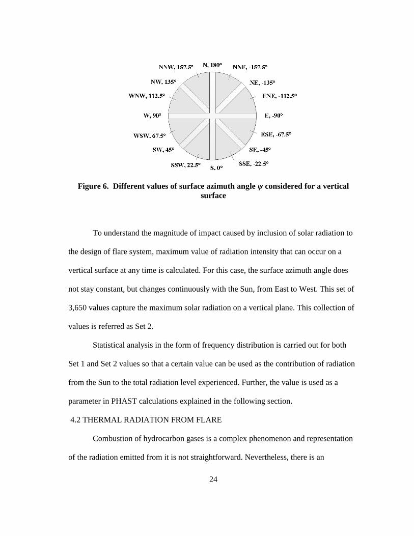
In addition to the time variation, radiation received by a surface would also vary

by changing surface azimuth angle ψ. Thus, to account for this change, radiation

intensity is calculated for 16 different azimuth angles, corresponding to 16 cardinal

directions as shown in Figure 6. This yields 3,650*16 values of radiation intensity. Let

this collection of values be called Set 1.

24

Figure 6. Different values of surface azimuth angle ψ considered for a vertical

surface

To understand the magnitude of impact caused by inclusion of solar radiation to

the design of flare system, maximum value of radiation intensity that can occur on a

vertical surface at any time is calculated. For this case, the surface azimuth angle does

not stay constant, but changes continuously with the Sun, from East to West. This set of

3,650 values capture the maximum solar radiation on a vertical plane. This collection of

values is referred as Set 2.

Statistical analysis in the form of frequency distribution is carried out for both

Set 1 and Set 2 values so that a certain value can be used as the contribution of radiation

from the Sun to the total radiation level experienced. Further, the value is used as a

parameter in PHAST calculations explained in the following section.

4.2 THERMAL RADIATION FROM FLARE

Combustion of hydrocarbon gases is a complex phenomenon and representation

of the radiation emitted from it is not straightforward. Nevertheless, there is an

25

abundance of models to calculate thermal radiation emitted by a fire. The radiation

models can be one of the following three types:

a. Semi-empirical models

b. Field models

c. Integral models

Field models are computationally intense as they are based upon solution of

Navier-Stokes equations averaged over time for momentum and mass. Semi-empirical

models are based on experimental results and are much simpler than field models.

Integral models are a middle ground between the other two models.

For evaluating hazards in a facility, semi-empirical methods provide reasonable

accuracy and are used in this study. Thermal radiation from flare is calculated by using a

hazard consequence modeling software PHAST developed by DNV-GL. It has an in-

built Radiation (RADS) jet flame model to predict thermal radiation intensity. It assumes

the fire geometry to be a conical frustum. The model is verified and validated against

experimental testing done by Chamberlain (1987) and Bennett et al (1991). Flare

modeling in PHAST is done as a “stand-alone” equipment item and the scenario is that

of a jet fire. The input to the scenario is mentioned below in Table 3 and is arranged

according to the tabs that appear when inputting data.

26

Table 3. Input data for PHAST simulation

S. No. Tab Group Field Value

1. Jet fire Jet fire model Jet fire model type Cone model

2.

Release

location

Elevation of discharge

point

25 m

3.

Release

characteristics

jet velocity 55 m/s

4.

Mass discharge rate 12.6 kg/s

5.

Two-phase release [unchecked]

6. Post-expansion jet

temperature

148.85 °C

7. Cone model

data

Cone model

data

Inclination of jet from

horizontal

45°

8.

Radiation

calculations

Type of

radiation

results

required

Radiation at a point [unchecked]

9.

Radiation vs distance [checked]

10.

Radiation ellipse [checked]

11.

Radiation contours [unchecked]

12. Radiation vs

distance

Transect Maximum distance 300 m

13.

Angle from release

direction

0°

14.

Height above origin 0 m

15.

Observer Fixed inclination [unchecked]

16.

Fixed orientation [unchecked]

17. Radiation

ellipse

Ellipse Ellipse type required Incident

radiation

18.

Specified radiation

intensity

1.58 and 4.73

kW/m2 (in

different

simulations)

19.

Observer Fixed inclination [unchecked]

27

For the study, radiation level of 4.73 kW/m2 and 1.58 kW/m2 as mentioned in

Table 1 are analyzed, since solar radiation is expected to be very less to make a

difference in the calculations for the rest of higher radiation levels.

Sample calculations from the Appendix of API 521 were adopted to be used for

flare specification in terms of mass discharge rate, flare temperature and average

molecular mass. A mixture of light hydrocarbons was assumed with average molar mass

of 46.1. Velocity was calculated based on Mach number of 0.2, which is an acceptable

design value for normal flow of gas from flare.

Height of the flare was assumed to be 25 m, which falls in the typical range of

height of the flare of 10-100 m. Some other inputs required before running the

simulation are presented in Table 4.

Table 4. Further input data for PHAST

Material (mol fraction)

Methane (0.08)

Propane (0.62)

n-Butane (0.30)

Wind Speed 5 m/s

Pasquill Stability D

Solar Radiation Intensity 0.85 kW/m2

28

4.3 EFFECT OF SOLAR RADIATION ADDITION

This section describes the procedure utilized in quantitatively measuring the

effect of including solar radiation in thermal radiation calculations by examining the

following factors:

4.3.1 EFFECT DISTANCE FROM THE FLARE BASE

Effect distance is the distance at the ground level from the base of the flare in the

downwind direction where a particular radiation level is experienced. Effect zone is the

circular area with its center as the flare base and the radius as the effect distance. Inside

this zone, the thermal radiation will exceed that particular level for the weather

conditions assumed and for any wind direction. Effect distance and the zone increases on

considering solar radiation for the radiation level of 4.73 kW/m2 and 1.58 kW/m2. This

depicts how much under-predicted the effect distance and hence the effect zone can be

when neglecting solar radiation.

4.3.2 HEIGHT OF FLARE STACK AND CORRESPONDING COST

If the facility layout is such that on considering solar radiation, the increased size

of the effect zone hinders with the placement of critical equipment/units, or if the

available space is limited, flare stack can be raised to an extent that the effect distance

remains unaltered even after the inclusion of solar radiation. This factor helps to

determine how high of a cost will have to be incurred for raising the flare stack in order

to restrict the effect zone to what it was when solar radiation was neglected. Equipment

cost of a self-supported flare can be estimated using equation 20 (Mussatti, Srivastava,

Hemmer, & Strait, 2002).

29

𝐶 = (9.14𝐷 + 0.749𝐿 + 78)2 (20)

where cost, C is in dollars

diameter of flare tip, D in inches

length, L of flare stack in feet

It is a representation of the cost of the stack along with some of its ancillary equipment.

Self-supported flare is designed for stack heights falling roughly in the range of 30-250

feet and the cost equation is developed for flare-tip diameter of 1-60 in. It has to be

borne in mind that the cost equation is developed using various quotes provided by

vendors and is believed to have an accuracy of ±30%.

4.3.3 PROBABILITY OF INJURY/FATALITY

To examine the extent of consequence of solar radiation contribution to thermal

radiation onto the personnel present in the vicinity of the flare stack, the probability of

them getting injured/killed is studied. The study is performed using probit equations. It

is believed that this statistical model is helpful both in the design phase and the risk

assessment phase of the flare system. However, probit equations prediction is not free of

uncertainties, one of the reasons being unpredictability of human reaction behavior to

radiation from fire.

TNO Green Book presents equation 21 and equation 22 for probability of fatality

and 2nd degree burns respectively, in terms of probit (Bosch & Twilt, 1992). The probit

can then be converted to percentage by using the erf function shown in equation 23 (De

Haag & Ale, 2005). The probits are based on the work done by Tsao and Perry (1979).

They made adjustment to probit based on nuclear explosion data.

30

𝑃𝑟𝑜𝑏𝑖𝑡𝑙𝑒𝑡ℎ𝑎𝑙𝑖𝑡𝑦 = 2.56 ln (𝐼

43t) − 36.38

(21)

𝑃𝑟𝑜𝑏𝑖𝑡20𝑏𝑢𝑟𝑛 = 3.0186 ln (𝐼

43t) − 43.14

(22)

where,

time of exposure, t is in seconds

radiation intensity, I is in W/m2

𝑃𝑟𝑜𝑏𝑎𝑏𝑖𝑙𝑖𝑡𝑦 = 0.5 [𝑒𝑟𝑓 (

𝑃𝑟𝑜𝑏𝑖𝑡 − 5

√2) + 1]

(23)

where,

erf (t) =

2

√𝜋∫ 𝑒−𝑥2

𝑑𝑥𝑡

0

(24)

The fatality probit developed by Lees is presented in equation 25 (Lees, 1994). In

the development of this probit, the progress made in medical treatment of burn injuries is

taken into account among other factors and the results obtained from the probit

somewhat differ from those obtained through TNO probit.

𝑃𝑟𝑜𝑏𝑖𝑡𝑙𝑒𝑡ℎ𝑎𝑙𝑖𝑡𝑦 = 1.99 ln (𝐼

43t∅

10,000) − 10.7

(25)

where, Φ is the clothing factor, φ = 0.5 in presence of clothing, and φ = 1 in absence of

clothing

Clothing can provide protection to bare skin from thermal radiation effects considerably,

if not ignited. The ignition of cloth takes place only at higher levels of radiation, higher

31

than 4.73 kW/m2 and 1.58 kW/m2 levels that are considered here for the study.

Therefore, while calculating the probits, protection provided by clothing should be

considered.

32

5 RESULTS AND DISCUSSION

5.1 SOLAR RADIATION

The analysis presented here has been performed for four different locations

namely: Brisbane (Australia), Edinburgh (Scotland), Houston (TX, USA) and Punta

Arenas (Chile). These locations were chosen to represent places in different hemispheres

of the world: northern, southern, eastern and western. For brevity and to avoid

repeatability, the results presented here are for Houston, TX, USA. Results for other

locations are shown in Appendix A.

5.1.1 SOLAR RADIATION WITH DIFFERENT ORIENTATION OF A

VERTICAL SURFACE

As discussed in Section 4.1.3, radiation intensity on a surface from the Sun

changes with the orientation of the surface. Personnel present near the flare, while

standing vertically, can be facing any direction. To capture this change along with the

change caused by time, radiation values are calculated for 16 different geographical

directions corresponding to different surface azimuth angles, ψ. Values for four of those

directions are shown in Figure 7, Figure 8, Figure 9 and Figure 10. All these figures

show the variation of solar radiation with time of the day when sunshine is received,

roughly from 0600 hrs. to 1900 hrs. Also, the different curves represent the variation in

radiation with different days of the year. Only four days out of 365 are illustrated, the 1st

day of January, April, July and October. For some figures, the solar radiation value for

hotter months is lesser, which does not seem intuitive. This is due to the altitude angle

33

being higher in summer which causes reduction in the value of direct solar radiation on a

vertical surface.

Figure 7. Solar radiation on a vertical surface facing South vs. time for different

days of the year

0

200

400

600

800

1000

5 6 7 8 9 10 11 12 13 14 15 16 17 18 19 20

Sola

r R

adia

tio

n W

/m2

Time (24-hr. format)

Vertical surface facing South, ψ = 0°

01-Jan 01-Apr 01-Jul 01-Oct

34

Figure 8. Solar radiation on a vertical surface facing North vs. time for different

days of the year

Figure 9. Solar radiation on a vertical surface facing East vs. time for different days

of the year

0

20

40

60

80

100

120

140

160

180

5 6 7 8 9 10 11 12 13 14 15 16 17 18 19 20

Sola

r R

adia

tio

n W

/m2

Time (24-hr. format)

Vertical surface facing North, ψ = 180°

01-Jan 01-Apr 01-Jul 01-Oct

0

100

200

300

400

500

600

700

800

5 6 7 8 9 10 11 12 13 14 15 16 17 18 19 20

Sola

r R

adia

tio

n W

/m2

Time (24-hr. format)

Vertical surface facing East, ψ = -90°

01-Jan 01-Apr 01-Jul 01-Oct

35

Figure 10. Solar radiation on a vertical surface facing West vs. time for different

days of the year

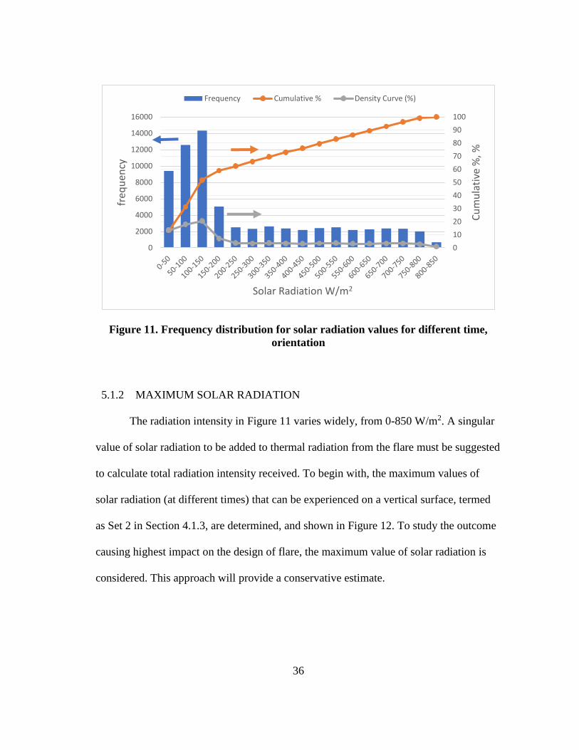
To understand the spread of solar radiation values, the frequency distribution of

Set 1 values mentioned in Section 4.1.3 is shown in Figure 11. These values correspond

to surfaces facing 16 different directions. For a surface to experience higher radiation, it

will have to directly face the sun, which does not have a high probability. That is the

reason of frequency being higher for lower values of radiation as depicted in Figure 11.

0

100

200

300

400

500

600

700

800

5 6 7 8 9 10 11 12 13 14 15 16 17 18 19 20

Sola

r R

adia

tio

n W

/m2

Time (24-hr. format)

Vertical surface facing West, ψ = 90°

01-Jan 01-Apr 01-Jul 01-Oct

36

Figure 11. Frequency distribution for solar radiation values for different time,

orientation

5.1.2 MAXIMUM SOLAR RADIATION

The radiation intensity in Figure 11 varies widely, from 0-850 W/m2. A singular

value of solar radiation to be added to thermal radiation from the flare must be suggested

to calculate total radiation intensity received. To begin with, the maximum values of

solar radiation (at different times) that can be experienced on a vertical surface, termed

as Set 2 in Section 4.1.3, are determined, and shown in Figure 12. To study the outcome

causing highest impact on the design of flare, the maximum value of solar radiation is

considered. This approach will provide a conservative estimate.

0

10

20

30

40

50

60

70

80

90

100

0

2000

4000

6000

8000

10000

12000

14000

16000

Cu

mu

lati

ve %

, %

freq

uen

cy

Solar Radiation W/m2

Frequency Cumulative % Density Curve (%)

37

Figure 12. Maximum solar radiation on a vertical surface vs. time for different

days of the year

Figure 13. Frequency distribution for maximum solar radiation, for different time

200

300

400

500

600

700

800

900

5 6 7 8 9 10 11 12 13 14 15 16 17 18 19 20

Sola

r R

adia

tio

n W

/m2

Time (24-hr. format)

Max. solar radiation on a vertical surface

01-Jan 01-Apr 01-Jul 01-Oct

0102030405060708090100

0100200300400500600700800900

1000

Cu

mu

lati

ve %

freq

uen

cy

Solar Radiation W/m2

frequency cumulative frequency % density curve

38

To understand the spread of maximum solar radiation values, the frequency

distribution of Set 2 values is shown in Figure 13. The same data is also presented in

Table 5. Set 2 is a subset of Set 1. The frequency of higher values of radiation is higher

because of Set 2 inherently containing all the maximum values of radiation occurring at

different times of the day.

Table 5. Frequency distribution table for maximum solar radiation at different

time

solar rad.

(W/m2) frequency

frequency

%

cumulative

frequency

%

0-50 34 0.78 0.78

50-100 55 1.25 2.03

100-150 54 1.23 3.26

150-200 79 1.80 5.06

200-250 73 1.66 6.72

250-300 57 1.30 8.02

300-350 174 3.97 11.99

350-400 116 2.64 14.63

400-450 141 3.21 17.85

450-500 192 4.38 22.22

500-550 251 5.72 27.95

550-600 237 5.40 33.35

600-650 298 6.79 40.14

650-700 397 9.05 49.19

700-750 628 14.32 63.51

750-800 897 20.45 83.95

800-850 704 16.05 100.00

39

As shown in Table 5, the maximum frequency of solar radiation values is for the range

of 750-800 W/m2. 800-850 W/m2 is also very close, with frequency percent of 16%.

Thus, a conservative value of 850 W/m2 is chosen to be the contribution to the total

radiation from the Sun. The same value can be taken for other places, Punta Arenas,

Edinburgh and Brisbane. Of course, the frequency of solar radiation values is not same

for these places, but that does not cause variation in picking the value of 850 W/m2. The

results for other locations are shown in Appendix A.

5.2 TOTAL THERMAL RADIATION

Radiation contribution from the Sun, as estimated in Section 5.1.2, is used as an

input in the radiation model of PHAST. Intensity radii and size of effect zone are used to

compare the consequence modeling results of the two cases of considering/not

considering solar radiation while calculating incident radiation.

As mentioned in Section 4.2, the incident radiation level of 4.73 kW/m2 and 1.58 kW/m2

are studied to compare the consequence analysis performed.

5.2.1 INTENSITY RADII AND EFFECT ZONE

Figure 14 and Figure 15 show the radiation ellipse (solid curve) and the effect

zone (dotted curve) for radiation level of 4.73 kW/m2. The same is listed in Table 6 for

both radiation levels of 4.73 kW/m2 and 1.58 kW/m2.

40

Figure 14. Radiation ellipse and effect zone discounting solar radiation

Figure 15. Radiation ellipse and effect zone considering solar radiation

41

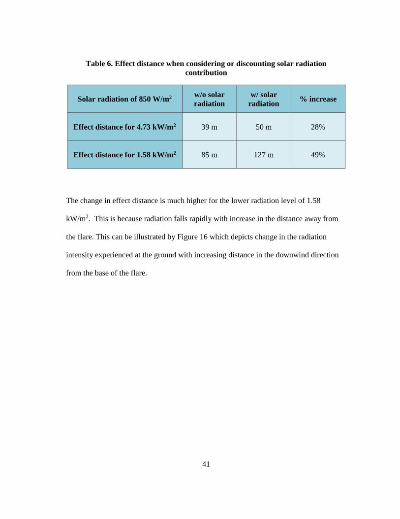
Table 6. Effect distance when considering or discounting solar radiation

contribution

Solar radiation of 850 W/m2 w/o solar

radiation

w/ solar

radiation % increase

Effect distance for 4.73 kW/m2 39 m 50 m 28%

Effect distance for 1.58 kW/m2 85 m 127 m 49%

The change in effect distance is much higher for the lower radiation level of 1.58

kW/m2. This is because radiation falls rapidly with increase in the distance away from

the flare. This can be illustrated by Figure 16 which depicts change in the radiation

intensity experienced at the ground with increasing distance in the downwind direction

from the base of the flare.

42

Figure 16. Total radiation intensity on the ground vs. distance downwind from the

flare base

5.2.2 FLARE HEIGHT

The outcome of considering solar radiation can also be studied by maintaining

the effect distance constant to the case when solar radiation is discounted, and increasing

the flare stack height, such that the radiation level of 4.73 kW/m2 and 1.58 kW/m2 is still

existent at the same distance from the flare. The increase in the stack height is shown in

Table 7. Subsequently, this will translate into an increment in the cost of the flare, which

is also tabulated.

0

1

2

3

4

5

6

0 25 50 75 100 125 150 175 200 225 250 275 300

Rad

iati

on

inte

nsi

ty, k

W/m

2

distance downwind, m

43

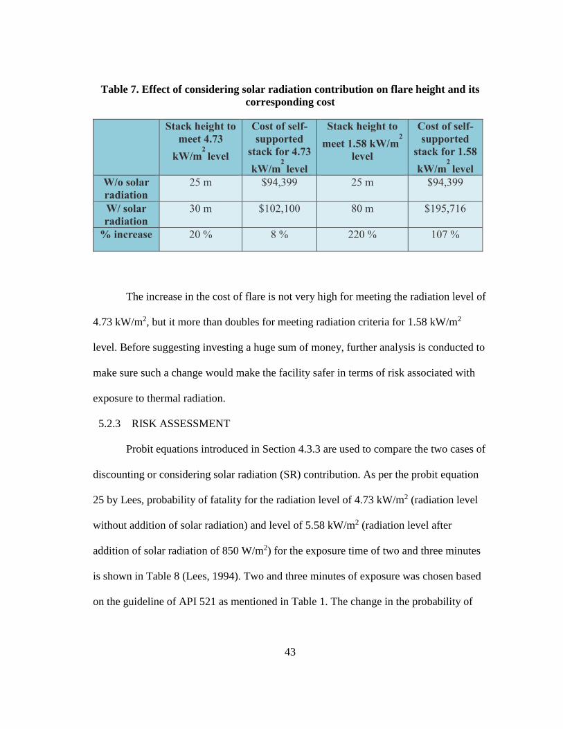
Table 7. Effect of considering solar radiation contribution on flare height and its

corresponding cost

Stack height to

meet 4.73

kW/m2

level

Cost of self-

supported

stack for 4.73

kW/m2

level

Stack height to

meet 1.58 kW/m2

level

Cost of self-

supported

stack for 1.58

kW/m2

level

W/o solar

radiation 25 m $94,399 25 m $94,399

W/ solar

radiation 30 m $102,100 80 m $195,716

% increase 20 % 8 % 220 % 107 %

The increase in the cost of flare is not very high for meeting the radiation level of

4.73 kW/m2, but it more than doubles for meeting radiation criteria for 1.58 kW/m2

level. Before suggesting investing a huge sum of money, further analysis is conducted to

make sure such a change would make the facility safer in terms of risk associated with

exposure to thermal radiation.

5.2.3 RISK ASSESSMENT

Probit equations introduced in Section 4.3.3 are used to compare the two cases of

discounting or considering solar radiation (SR) contribution. As per the probit equation

25 by Lees, probability of fatality for the radiation level of 4.73 kW/m2 (radiation level

without addition of solar radiation) and level of 5.58 kW/m2 (radiation level after

addition of solar radiation of 850 W/m2) for the exposure time of two and three minutes

is shown in Table 8 (Lees, 1994). Two and three minutes of exposure was chosen based

on the guideline of API 521 as mentioned in Table 1. The change in the probability of

44

fatal injury does not change at all or changes negligibly upon consideration of solar

radiation contribution.

Table 8. Probability of fatality per Lees probit equation for radiation level of 4.73

kW/m2 (with or without SR)

q, W/m2 t, s Probit Fatal

probability

no SR 4730 120 1.57 0.00

SR=850 W/m2 5580 120 2.00 0.00

no SR 4730 180 2.38 0.00

SR=850 W/m2 5580 180 2.82 0.01

Similar analysis as above is repeated using probit equation of the TNO Green

Book and shown in Table 9. The fatality obtained by the probit equation 21 is reduced

by multiplying by a factor of 0.14 to account for the protective effect of clothing (Bosch

& Twilt, 1992).

Table 9. Probability of fatality per Green Book probit equation for radiation level

of 4.73 kW/m2 (with or without SR)

-- q, W/m2 t, s Probit

Fatal

probability

(no clothing)

Fatal

probability

(with clothing)

no SR 4730 120 4.76 0.40 0.06

45

Table 9. Continued

q, W/m2 t, s Probit

Fatal

probability

(no clothing)

Fatal

probability

(with clothing)

SR=850

W/m2 5580 120 5.32 0.63 0.09

no SR 4730 180 5.80 0.79 0.11

SR=850

W/m2 5580 180 6.36 0.91 0.13

Table 10. Probability of 2nd degree burn per Green Book probit equation for

radiation level of 4.73 kW/m2 (with or without SR)

q, W/m2 t, s Probit

Probability

for 2nd degree

burn (no

clothing)

Probability for

2nd degree

burn (with

clothing)

no SR 4730 120 5.37 0.64 0.09

SR=850

W/m2 5580 120 6.03 0.85 0.12

no SR 4730 180 6.59 0.94 0.13

SR=850

W/m2 5580 180 7.26 0.98 0.14

The increase in the probability of a fatal injury for radiation level of 4.73 kW/m2

(from no SR to considering SR = 850 W/m2) is not very significant. It increases from 6%

to 9% for 120 s. of exposure, and from 11% to 13% for 180 s. of exposure. Similarly, the

probability of 2nd degree burns, as shown in Table 10, has not notably increased. It

should be noted that these fatality/injury probability numbers are further multiplied to

46

other probabilities, like probability of a person present in the concerned area and

probability of the wind speed prevailing at the time. when performing a full-blown risk

assessment. Therefore, the impact to the sustained risk by disregarding solar radiation

contribution would be diminished further.

The probit equations presented in the TNO book is based on the work done by

Tsao and Perry (Tsao & Perry, 1979). They made modifications to the vulnerability

model developed by Eisenberg et al who put forward the probit on the basis of radiation

injuries caused by the nuclear explosions (Eisenberg, Lynch, & Breeding, 1975).

Although, Tsao and Perry made adjustment to their model to account for the difference

in extent of injuries caused by infrared radiation (from hydrocarbon fire) rather than UV

and visible radiation (from nuclear explosions), some other conditions and assumptions

remain the same. For example, the treatment of burn injuries and fatalities have

improved significantly since 1975. Also, the probit results are based on the injuries

caused to all the age groups, including children and older people. Both these groups are

more vulnerable to burn injury in comparison to the people belonging to the typical

working-age class. In addition, TNO considers protection provided by clothing based on

the average population statistics of Netherlands, which again includes younger and older

population. Hence, all these attributes make the TNO probit equation conservative in

predicting thermal radiation effects on personnel.

On the other hand, Lees probit equation incorporates more recent advancements

in medical treatment and knowledge of intensity of the burns (Lees, 1994). The

population considered also lies in the age category of 10-69 years, thus discounting the

47

more vulnerable categories of children and older people. Hence, the Lees probit equation

seems to be a better representation of the probability of fatality from thermal radiation,

shown in Table 8.

Therefore, for the suggested level of 4.73 kW/m2 by API 521, for which

emergency action may be performed by personnel clad in proper clothing lasting about

2-3 minutes, a disregard for solar radiation does not significantly alter the probability of

fatality. Also, the probability of 2nd degree burns as shown in Table 10 does not increase

by a considerable extent.

Similar analysis is also performed for the radiation level of 1.58 kW/m2, for

which API 521 suggests that the personnel can be present in that area for extended

periods of time. However, using Lees probit for an exposure time of 1 hr. and 2 hrs.

yields very high probability of fatality, as shown in Table 11, which seems to be

unlikely.

Table 11. Probability of fatality per Lees probit equation for radiation level of 1.58

kW/m2 (with or without SR)

q, W/m2 t, s Probit Fatal

probability

no SR 1580 3600 5.43 0.67

SR=850 W/m2 2430 3600 6.57 0.94

no SR 1580 7200 6.81 0.96

SR=850 W/m2 2430 7200 7.95 0.99

48

It has been discussed previously that using probit relations at extremes can result

in overly conservative estimates (Daycock & Rew, 2000). A very high exposure time

will result in a high thermal dose (dose = q4/3t) even when the radiation intensity is low,

as shown in the case of radiation level of 1.58 kW/m2. Moreover, the experiments/data

used to develop these probit equations have exposure time of a few seconds, and not

hours. Thus, the conclusion drawn from probit for extended exposure time is not

reliable.

Since, radiation level of 1.58 kW/m2 is too low to cause fatality, another method

to measure heat stress caused by continuous exposure can be utilized: an index for the

assessment of hot environments. One such empirical index is Wet Bulb Globe

Temperature (WBGT) which is extensively used and is also presented in ISO Standard

7243 (International Standards Organization, 1982). WBGT is measured using instrument

on site, but can also be calculated fairly accurately using available weather data as done

by Liljegren et al (2008). Software1 has been developed which has automated the

calculations and only requires weather data as input (Liljegren, 2008). Input as shown in

Table 12 was used for Houston, TX when considering solar radiation in the calculations.

1 Copyright © 2008, UChicago Argonne LLC, All Rights Reserved, Wet Bulb Globe Temperature

(WBGT) Version 1.2, Author: James Liljegren, Argonne National Laboratory, DIS Divison.

49

Table 12. Input and output in software used to calculate WBGT, considering solar

radiation

Air temperature 28.9 °C

Solar irradiance 850 W/m2

Wind speed 5 m/s

Relative humidity 50%

Atmospheric pressure 1009.4 millibar

WBGT obtained 26.3 °C

The air temperature considered is the maximum average temperature for Houston

(ASHRAE Standard Committee, 2013).

Since clothing restricts evaporative cooling of the body, and tends to increase

core body temperature, effective WBGT (WBGTeff) is obtained by adding clothing

adjustment factor (CAF) to the WBGT, both expressed in degree Celsius. Refer to Table

13 for the same. (American Conference of Governmental Industrial Hygienists, 2017).

For this study, clothing is taken as normal cotton work clothes, for which WBGTeff =

WBGT.

50

Table 13. Clothing adjustment factor to WBGT

Clothing Worn CAF

Work clothes (long sleeves and pants). Examples: Standard cotton

shirt/pants. 0

Coveralls (w/only underwear underneath). Examples: Cotton or light

polyester material. 0

Double-layer woven clothing. 3

SMS Polypropylene Coveralls 0.5

Polyolefin coveralls. Examples: Micro-porous fabric (e.g., Tyvek™). 1

Limited-use vapor-barrier coveralls. Examples: Encapsulating suits,

whole-body chemical protective suites, firefighter turn-out gear. 11

Metabolic rate (MR) of personnel should also be known to calculate heat stress.

It can be estimated by using equation 26 (American Conference of Governmental

Industrial Hygienists, 2017). Body weight is assumed to be 70 kg for simplification and

Table 14 is referred to know work expectation (in Watts) (American Conference of

Governmental Industrial Hygienists, 2017). Moderate work expectation from the worker

is assumed, which translates to 300 W. Threshold limit values (TLV) for different types

of workload are suggested in Table 15, and if WBGTeff exceeds the TLV, worker is

believed to be under risk due to heat stress and exhaustion (American Conference of

Governmental Industrial Hygienists, 2017). Nevertheless, it should be kept in mind that

TLV is just a screening tool. When WBGTeff does exceed TLV, further detailed analysis,

e.g., physiological monitoring should be performed.

51

𝑀𝑅 = 𝑊𝑜𝑟𝑘 𝑒𝑥𝑝𝑒𝑐𝑡𝑎𝑡𝑖𝑜𝑛 (𝑖𝑛 𝑊𝑎𝑡𝑡𝑠) ×𝑤𝑜𝑟𝑘𝑒𝑟 𝑏𝑜𝑑𝑦 𝑤𝑒𝑖𝑔ℎ𝑡 (𝑖𝑛 𝑘𝑔)

70 𝑘𝑔 (26)

Table 14. Work expectation in terms of different work category

Work

Category

Work expectation

(Watts) Examples

Rest 115 Sitting

Light 180 Sitting, standing, light arm/hand work

and occasional walking

Moderate 300 Normal walking, moderate lifting

Heavy 415 Heavy material handling, walking at a

fast pace

Very Heavy 520 Pick and shovel work

Table 15. Threshold limit Values (TLV) for different work load and different

work/rest regime

% Work Workload/ Work expectation

Light Moderate Heavy Very Heavy

75 to 100%

(Continuous)

31.0°C 28.0°C N/A N/A

50 to 75% 31.0°C 29.0°C 27.5°C N/A

25 to 50% 32.0°C 30.0°C 29.0°C 28.0°C

0 to 25% 32.5°C 31.5°C 30.5°C 30.0°C

52

Even for continuous work, and moderate workload as assumed, TLV is 28 °C

from Table 15, and WBGTeff = 26.3 °C from Table 12, which does not exceed TLV.

Therefore, even with considering solar radiation, workers are at a significantly low risk

of heat stress.

53

6 CONCLUSIONS AND RECOMMENDATIONS

The study carried out here tries to quantitatively address the variation of either

considering or disregarding solar radiation when designing flare based on allowed

thermal radiation levels on the ground. Since, the objective of the study was to develop a

framework that helps in making the most suitable decision for the specific facility, the

conclusions drawn here are relevant when the same data and assumptions hold true at the

site. Nevertheless, the framework can still be applied in other cases, and conclusions

drawn based on results thus obtained.

Radiation level of 4.73 kW/m2 and 1.58 kW/m2 are studied for this assessment,

and the two cases of zero solar radiation (SR) contribution and solar radiation

contribution of 850 W/ m2 are compared. It is worth noting that 850 W/m2 is the

maximum value of solar radiation that may exist at any time on a vertical plane.

• For radiation level of 4.73 kW/m2, consideration of SR demands either a 28%

increase in the effect distance as shown in Table 6, which translates to a 64%

increase in the effect zone, or an increase in flare height causing the flare cost to

increase by 8% as shown in Table 7. However, on doing so, the risk to personnel

in terms of reduction of the probability of death/second degree burn shown in

Table 8 and Table 10 is not significant.

• For radiation level of 1.58 kW/m2, consideration of SR demands either a 49%

increase in the effect distance as shown in Table 6, which translates to a 122%

increase in the effect zone, or an increase in flare height causing the flare cost to

54

increase by 107% as shown in Table 7. The increase in design values is too high.

The decision of accounting for SR should not be made without assessing the

actual outcome of neglecting SR. This is done by estimating heat stress

experienced by a worker. Since WBGT, which is a heat index extensively used,

calculated and shown in Table 12, is below the TLV discussed in Table 15, SR

can be safely neglected without compromising the safety of the workers exposed.

That being said, WBGT did not exceed TLV for the given weather data, where

air temperature is assumed to be the maximum average monthly temperature for

Houston, TX. It is possible that some days are hotter and WBGT exceeds TLV

on those days. In that case, exercising general controls at the site will be much

more feasible in maintaining safe working environment in contrast to designing

the flare system with the absolute worst conditions which have a very low

probability of occurrence and still do not lend notable reduction in the risk level.

General controls include, an appropriate work/rest regime where workers take

few minutes break during every hour, physiological monitoring of the workers

and an improved awareness about the symptoms to look out that suggest heat

exhaustion.

After carrying the analysis explained in this study, it can be concluded that

solar radiation contribution can be discounted while designing flare based on 4.73

kW/m2 and 1.58 kW/m2 radiation level. Even after taking the highest value of solar

radiation, the apparent risk reduction is not remarkable to justify the immense increase in

design factors. When designing a flare, this can further be confirmed by using the

55

conditional probability data for the quantitative risk assessment (QRA) performed for the

flare system. QRA uses conditional probability of rest of the factors, like, weather and

wind direction probability, probability of the person present in the area where particular

radiation level exists. Using this information, risk posed on the facility in terms of

fatalities/injuries per year can be computed and compared. For heat stress values, the

data and conclusions presented in the study can further be stated with enhanced

confidence by measuring WBGT with the help of meteorological data of the particular

site, or better still using WBGT monitors installed on workers’ bodies.

56

REFERENCES

American Conference of Governmental Industrial Hygienists. (2017). TLVs and BEIs

Threshold Limit Values for Chemical Substances and Physical Agents and

Biological Exposure Indices

American Petroleum Institute. (2007). API 521 Pressure-relieving and depressuring

systems.

American Petroleum Institute. (2008). API 537- Flare Details for General Refinery and

Petrochemical Service.

ASHRAE Standard Committee. (2013). Chapter 14: Climatic Design Information. In

ASHRAE Handbook: Fundamentals

Bamber, J. L., & Payne, A. J. (2004). Mass balance of the cryosphere: observations and

modelling of contemporary and future changes: Cambridge University Press.

Banerjee, K., Cheremisinoff, N. P., & Cheremisinoff, P. N. (1985). Flare gas systems

pocket handbook: Gulf Publishing.

Baukal Jr, C. E. (2012a). The John Zink Hamworthy Combustion Handbook. In (2nd

ed., Vol. 3, pp. 253). Boca Raton: CRC Press.

Baukal Jr, C. E. (2012b). The John Zink Hamworthy Combustion Handbook. In (2nd

ed., Vol. 1, pp. 480-512). Boca Raton: CRC press.

Baukal Jr, C. E. (2012c). The John Zink Hamworthy Combustion Handbook. In (2nd

ed., Vol. 3, pp. 251-297). Boca Raton: CRC Press.

Baukal Jr, C. E. (2012d). The John Zink Hamworthy Combustion Handbook. In (2nd

ed., Vol. 1, pp. 207-225). Boca Raton: CRC press.

57

Bennett, J., Cowley, L., Davenport, J., & Rowson, J. (1991). Large scale natural gas and

LPG jet fires final report to the CEC. Shell report TNER, 91.

Bosch, C. J. H. v. d., & Twilt, L. (1992). Damage caused by heat radiation. In Methods

for the determination of possible damage to people and objects resulting from

releases of hazardous materials Report CPR E (Vol. 16): TNO - The

Netherlands Organisation of Applied Scientific Research.

Chamberlain, G. (1987). Developments in design methods for predicting thermal

radiation from flares. Chemical Engineering Research and Design, 65(4), 299-

309.

Cooper, P. (1969). The absorption of radiation in solar stills. Solar energy, 12(3), 333-

346.

Daycock, J., & Rew, P. (2000). Thermal radiation criteria for vulnerable populations:

HSE Books.

De Haag, P. U., & Ale, B. (2005). Guidelines for Quantitative Risk Assessment: Purple

Book: Ministerie van Volkshuisvesting en Ruimtelijke Ordening (VROM).

Eisenberg, N. A., Lynch, C. J., & Breeding, R. J. (1975). Vulnerability model. A

simulation system for assessing damage resulting from marine spills.

Gueymard, C. A. (2008). REST2: High-performance solar radiation model for cloudless-

sky irradiance, illuminance, and photosynthetically active radiation–Validation

with a benchmark dataset. Solar energy, 82(3), 272-285.

Hajek, J. D., & Ludwig, E. E. (1960). How to Design Safe Flare Stacks. Petro/Chem

Engineer, 32(6), C31–C38.

58

International Standards Organization. (1982). Hot Environments- estimation of heat

stress on working man based on the WBGT (Wet Bulb Globe Temperature)

index ISO 7243.

Iqbal, M. (1983). An introduction to solar radiation. Ontario, Canada: Academic Press.

Johnson, A., Brightwell, H., & Carsley, A. (1994). A model for predicting the thermal

radiation hazards from large-scale horizontally released natural gas jet fires.

Process safety and environmental protection, 72, 157-166.

Kasten, F., & Young, A. T. (1989). Revised optical air mass tables and approximation

formula. Applied optics, 28(22), 4735-4738.

Kreith, F., & Kreider, J. F. (1978). Principles of solar engineering: HemispherePub.

Corp.

Lees, F. P. (1994). The assessment of major hazard: a model for fatal injury from burns.

Process safety and environmental protection, 72(3), 127-134.

Liljegren, J. C. (2008). Wet Bulb globe Temperature (WBGT) (Version 1.2): Argonne

National Laboratory, DIS Division.

Liljegren, J. C., Carhart, R. A., Lawday, P., Tschopp, S., & Sharp, R. (2008). Modeling

the wet bulb globe temperature using standard meteorological measurements.

Journal of occupational and environmental hygiene, 5(10), 645-655.

McMurray, R., Oswald, B. J., & Witheridge, R. E. (1980). A Guide To Flare System

Design, With Particular Reference To Offshore Platforms. Paper presented at the

Offshore Technology Conference.

59

Mussatti, D. C., Srivastava, R., Hemmer, P. M., & Strait, R. (2002). EPA air pollution

control cost manual. Air Quality Strategies and Standards Division of the Office

of Air Quality Planning and Standards, US Environmental Protection Agency,

Research Triangle Park, NC, 27711.

Oenbring, P., & Sifferman, T. (1980). Flare design... are current methods too

conservative. Hydrocarbon Processing, 60(5), 124-129.

Schwartz, R. E., & Kang, S. G. (1998). Flare System Design- What is Important?

Stephenson, D. G. (1965). Equations for solar heat gain through windows. Solar energy,

.9(2), 81-86.

Thevenard, D., & Haddad, K. (2006). Ground reflectivity in the context of building

energy simulation. Energy and buildings, 38(8), 972-980.

Threlkeld, J. L. (1963). Solar irradiation of surfaces on clear days. ASHRAE

Transactions, 69, 24-36.

Tsao, C. K., & Perry, W. W. (1979). Modifications to the vulnerability model: A

simulation system for assessing damage resulting from marine spills (CG-D-38-

79). Retrieved from Washington, D. C. 20590.

60

APPENDIX

Here, the values of solar radiation existing at different times at Punta Arenas

(Chile), Edinburgh (Scotland) and Brisbane (Australia) are presented in the said order.

Figure 17, Figure 18 and Figure 19 show the frequency distribution of SR values in Set

1, comprising of SR values corresponding to the surface facing 16 different directions.

Figure 17. Frequency distribution for solar radiation values for different time,

orientation for Punta Arenas, Chile

0102030405060708090100

0

2000

4000

6000

8000

10000

12000

14000

16000

18000

Cu

mu

lati

ve %

freq

uen

cy

Solar Radiation W/m2

frequency cumulative % Density curve (%)

61

Figure 18. Frequency distribution for solar radiation values for different time,

orientation for Edinburgh, Scotland

Figure 19. Frequency distribution for solar radiation values for different time,

orientation for Brisbane, Australia

0102030405060708090100

02000400060008000

100001200014000160001800020000

Cu

mu

lati

ve %

freq

uen

cy

Solar Radiation W/m2

Frequency Cumulative % Density curve (%)

0102030405060708090100

0

2000

4000

6000

8000

10000

12000

14000

16000

Cu

mu

lati

ve %

freq

uen

cy

Solar Radiation W/m2

Frequency Cumulative % Density curve (%)

62

To adopt a more conservative approach in choosing the SR contribution,

frequency distribution for Set 2 values is shown in Figure 20, Figure 21 and Figure 22

for Punta Arenas, Edinburgh and Brisbane respectively. The analysis done for picking

850 W/m2 as SR contribution for Houston is also valid for these locations. For Punta

Arenas, there are some values which are in the range of 850-900 W/m2. 7% of the total

SR values fall in the range of 850-900 W/m2 as compared to a much higher 27% of the

total SR values falling in the range of 800-850 W/m2. Therefore, the decision of picking

850 W/m2 as SR contribution is still justified.

Figure 20. Frequency distribution for maximum solar radiation, for different time

at Punta arenas, Chile

0102030405060708090100

0

200

400

600

800

1000

1200

1400

Cu

mu

lati

ve %

freq

uen

cy

Solar Radiation W/m2

Frequency Cumulative % Density curve (%)

63

Figure 21. Frequency distribution for maximum solar radiation, for different time

at Edinburgh, Scotland

Figure 22. Frequency distribution for maximum solar radiation, for different time

at Brisbane, Australia

0102030405060708090100

0

200

400

600

800

1000

1200

Cu

mu

lati

ve %

freq

uen

cy

Solar Radiation W/m2

Frequency Cumulative % Density curve (%)

0102030405060708090100

0100200300400500600700800900

1000

Cu

mu

lati

ve %

freq

uen

cy

Solar Radiation W/m2

Frequency Cumulative % Density curve (%)