Embed Size (px)
Citation preview

THINK IN G MACHINES CORPORATION
CONNECTION MACHINE TECHNICAL SUMMARY

TheConnection MachineSystem
Connection MachineModel CM-2 Technical Summary
.................................................................
Version 6.0November 1990
Thinking Machines CorporationCambridge, Massachusetts

First printing, November 1990
The information in this document is subject to change without notice and should not be construedas a commitment by Thinking Machines Corporation. Thinking Machines Corporation reservesthe right to make changes to any products described herein to improve functioning or design.Although the information in this document has been reviewed and is believed to be reliable,Thinking Machines Corporation does not assume responsibility or liability for any errors that mayappear in this document. Thinking Machines Corporation does not assume any liability arisingfrom the application or use of any information or product described herein.
Connection Machine® is a registered trademark of Thinking Machines Corporation.CM-1, CM-2, CM-2a, CM, and DataVault are trademarks of Thinking Machines Corporation.C*® is a registered trademark of Thinking Machines Corporation.Paris, *Lisp, and CM Fortran are trademarks of Thinking Machines Corporation.C/Paris, Lisp/Paris, and Fortran/Paris are trademarks of Thinking Machines Corporation.VAX, ULTRIX, and VAXBI are trademarks of Digital Equipment Corporation.Symbolics, Symbolics 3600, and Genera are trademarks of Symbolics, Inc.Sun, Sun-4, SunOS, and Sun Workstation are registered trademarks of Sun Microsystems, Inc.UNIX is a registered trademark of AT&T Bell Laboratories.The X Window System is a trademark of the Massachusetts Institute of Technology.StorageTek is a registered trademark of Storage Technology Corporation.Trinitron is a registered trademark of Sony Corporation.
Copyright © 1990 by Thinking Machines Corporation. All rights reserved.
Thinking Machines Corporation245 First StreetCambridge, Massachusetts 02142-1264(617) 234-1000/876-1111

Contents..? ,' ;. ...,. I--I~-...... >,.s;
Part I The Parallel Environment
Parallel Architecture......................
System Organization ...........................
Data Parallel Hardware ........................
Data Parallel Computation ......................
Data Parallel Software .........................
The Operating System Environment.The Front-End Environment ....................
Partitioning the Connection Machine System .......
The NQS Batch System ........................
Timesharing ..................................
The Program Development Environment ..........
The Program Execution Environment .............
The Connection Machine File System .............
CM Diagnostics ..............................
Part II Parallel Software
Languages ............................Establishing Parallel Data Structures .........
Establishing Linkages among Data Elements ..
Establishing Scalar Data ...................
Operations on Mixed Data .................
Conditionals ............................
111
Chapter 11.1
1.2
1.31.4
Chapter 22.12.22.32.4
2.5
2.6
2.7
2.8
334
7
12
13
131415
17
17
1819
20
Chapter 33.1
3.2
3.3
3.4
3.5
2324
24
25
25
25
.................
.................
.................
.................
.................
.................
.................
.................
.................
.................
.................
.................
.................
.................
.................
.................
.................
.................
.................
.................

iv Connection Machine Model CM-2 Technical Summary
Fortran .....................Structuring Parallel Data .........
Computing in Parallel ............
Communicating in Parallel ........
Transforming Parallel Data .......
To Learn More .................
The C* Language .........Structuring Parallel Data .......
Computing in Parallel ..........
Communicating in Parallel ......
Transforming Parallel Data .....
The *Lisp Language ....
Structuring Parallel Data .....
Computing in Parallel ........
Communicating in Parallel ....
Transforming Parallel Data ...
r 7 CM Scientific Software Library ...
7.1 CMSSL Capabilities ....................
7.2 CMSSL Parallel Computation ............
7.3 Linear Algebra ........................
7.4 Fast Fourier Transforms .................
7.5 Random Number Generators .............
7.6 Statistical Analysis .....................
Data Visualization .................
Visualization Output from the CM System..
*Render ..............................
Generic Display Interface ...............
Image File Interface ....................
27
27
29
30
32
33
35
35
37
38
40
Chapter 44.1
4.2
4.3
4.4
4.5
Chapter 55.1
5.2
5.3
5.4
Chapter 66.1
6.2
6.3
6.4
Chaptei
Chapter 88.1
8.28.3
8.4
41
42
45
46
48
51
51
53
56
58
59
60
61
62
63
65
67
Connection Machine Model CM-2 Technical Summaryiv
...........
...........
...........
...........
...........
...........
....................
....................
....................
....................
....................
....................
.............
.............
.............
.............
.............
..........
..........
..........
..........
..........
..........
..........
..........
..........
..........
.............
.............
.............
.............
.............
............
............
............
............
............
..........
..........
..........
..........
..........
........................
........................
........................
........................
........................
........................
........................
........................
........................
........................
........................
........................

C.nn Vr. - - - - - - -- - -
Part m Parallel Architecture
Paris .......................................................
Virtual Machine Archiectu .....................................
9.2 Instruction Set Overview ......................
Chapter 10 CM-2 Architecture ..............10.1 Processor Architecture ...............
10.210.3
10.410.5
10.610.7
The Parallel Processing Array ........
The Floating-Point Accelerator ........
The Router ........................
The NEWS Grid ....................
Scans and Spreads ..................Communication with the Front End ....
Chapter 1111.1
11.211.311.411.5
Chapter 1212.112.212.3
Chapter 1313.113.213.3
Chapter 1414.1
14.2
Data and Image UO ......................Data I/O Channels ............................Data I/O Overview ............................
Graphics Output for Data Visualization ...........CM I/O Controller ............................CMIO Bus ...................................
The DataVault ............................
The File Server ...............................
Writing and Reading Data ......................Data Protection ...............................
9191
92
93
93
94
................. .97
................. 99
................. 100
................. 101
CMIO Intelligent Bus Interfaces ..HIPPI Bus Interface ....................VMEbus Interface......................SCSI Bus Interface .....................
103103
104
105
The Graphics Display System .....Connection Machine Framebuffer .........The Monitor..........................
107107
109
Chapter 99.1
71
71
75
81
838385
86888990
Contents v
.....................................................
........................................ ............
.. .. ..
.........
.... ...
.........
... ... .. ... .......... ........
........ ........
........ ........
...... ........... .....
................. ... ...
....... ....... .......
.... .... .... .... ...
........................

v i
··I· ·:i
i�-� an P
..:.:··3-i -;·I:; ,.----- :i- ·�- :· ·-�
:? �'� i::
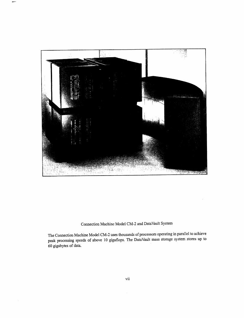
Connection Machine Model CM-2 and DataVault System
The Connection Machine Model CM-2 uses thousands of processors operating in parallel to achieve
peak processing speeds of above 10 gigaflops. The DataVault mass storage system stores up to
60 gigabytes of data.
vii

Part IThe Parallel Environment

2.

Chapter 1
Parallel Architecture
The Connection Machine Model CM-2 is a data parallel computing system. Data parallelcomputing associates one processor with each data element. This computing style exploitsthe natural computational parallelism inherent in many data-intensive problems. It can sig-nificantly decrease the execution time of a problem, as well as simplify its programming.Execution time is frequently reduced in proportion to the number of data elements in thecomputation; programming effort is reduced in proportion to the complexity involved inexpressing a naturally parallel problem statement in a serial manner.
The Connection Machine Model CM-2 is an integrated system of hardware and software.The hardware elements of the system include front-end computers that provide the devel-opment and execution environments for the users' software, a parallel processing unit of64K processors that executes the data parallel operations, and a high-performance dataparallel I/O system. Software elements begin with the standard operating system andprogram development environment of the front-end computer and enhance that environ-ment with extensions to standard languages and tools that facilitate data parallel programdevelopment. Users write programs using familiar languages and constructs, taking advan-tage of the full, enhanced front-end development environment. When they choose, they canalso call on CM language features and library routines specifically designed to handle tasksand problems germane to large-scale data-intensive programming. Programs have normalsequential control flow; new synchronization structures are not needed. Thus, users caneasily develop programs that exploit the power of the Connection Machine hardware.
1.1 System Organization
The Connection Machine system was specifically designed to handle the largest computa-tional problems. At the heart of any large computational problem is its data set: somecombination of related data objects, such as numbers, characters, records, structures, and
3

4 CnnctonMahie odl M- Tchicl umar
arrays. The task of any application is to select, combine, rearrange, and operate upon thisdata. Data-level parallelism expedites this task by taking advantage of the parallelisminherent in large data sets.
At the heart of the Connection Machine system is the parallel processing unit, which con-sists of up to 64K processors, each with up to 128 kilobytes of memory. These processorscan not only process the data stored in their memory, but also can exchange informationamong themselves and with I/O peripherals. All these operations happen in parallel on allprocessors.
A CM-2 parallel processing unit may contain 16K, 32K, or 64K data processors. The modelCM-2a may contain 4K or 8K data processors. Here, and throughout this document, 'K"stands for 1024, or 210. Thus 64K means 65,536; 32K means 32,768; 16K means 16,384;8K means 8,192; and so on.
The Connection Machine processors are used whenever an operation can be performedsimultaneously on many data objects. Data objects remain in the Connection Machinememory during execution of the program and are operated upon in parallel. This modeldiffers from the serial model, where data objects in a computer's memory are processedone at a time, by reading each one in turn, operating on it, and then storing the result backin memory before processing the next object.
Of course, some small part of an application's data may be better processed serially. Suchdata resides in the memory of the front-end computer and is processed serially in the usualway. The memories of the parallel processors hold the bulk of data that can be usefullyprocessed in parallel. The flow of control is handled entirely by the front end, includingstorage and execution of the program and all interaction with the user and/or programmer.Parallel data is operated upon through commands sent by the front end to the ConnectionMachine processors.
1.2 Data Parallel Hardware
The Connection Machine system implements data parallel programming constructs direct-ly in hardware and microcode. Parallel data structures are spread across the dataprocessors, with a single element stored in each processor's memory. When parallel datastructures contain more data elements than the system has processors (the normal situ-ation), the system operates in virtual processor mode, presenting the user with a largernumber of processors, each with a correspondingly smaller memory. This allows the userto write programs assuming the number of processors that is natural for the application,rather than forcing code to conform to the number of hardware processors available. Each
-
Connection Machine Model CM-2 Technical Summary4

Chapter 1. Parallelgrchitecture 5
hardware processor is made to simulate the appropriate number of virtual processors; as theprogram issues each parallel instruction, microcode causes it to be executed many times,once for each virtual processor. The same program can run without change on differentquantities of hardware processors-but the more hardware, the faster it runs.
Interprocessor communication is implemented by a special-purpose high-speed network.When data is needed, it is passed over the network to the appropriate processors. Proces-sors that hold interrelated data elements store pointers to one another, thus supportingcompletely general patterns of communication. In addition, special hardware supports cer-tain commonly used regular patterns of communication. Nearest-neighbor communicationin a multidimensional rectangular grid is particularly efficient.
High-speed transfers between peripheral devices and Connection Machine memory takeplace through the Connection Machine I/0 system. All processors, in parallel, pass data toand from I/O buffers. The data is then moved between the buffers and the peripheraldevices. Connection Machine high-speed peripherals include the DataVault mass storagesystem, the Connection Machine graphics display system, the Connection Machine VMEI/0 system, and the HIPPI high-speed interface.
Chapter . Parallel Architecture 5

.6.. ::... .. ,.C nt -~. T:e.:. ......................................... ..::. : ' : .: �chnicl::.'u ay. ...::.. I .... .'.:.......: X...':':.:.:::.. e'.-.-p ........... . ... . ~ ~ ~ ~ ~ ~ :
Figure 1. Components of a Connection Machine system. The user's terminal
provides access to the front-end computer, CM-2 parallel processing unit,DataVaults, and high-resolution graphics color monitors.
Connection Machine Model CM-2 Technical Summary6

Chapter 1. Parallelrchitecture 7
1.3 Data Parallel Computation
Connection Machine systems are designed to operate on large amounts of data. These datasets may be richly interconnected or totally autonomous. A scientific simulation data set,such as a finite-element grid, is highly interconnected, with every node value connected toseveral element values and vice versa. Disparate values are continually being broughttogether, computed on, and redispersed. A document data base, on the other hand, may betotally autonomous. The search of any one document proceeds entirely without referenceto any of the others. There is no need to combine information from multiple documents ina single computation.
The Connection Machine system is made up of large numbers of processors, each with itsown local memory. (Note that a system with 65,536 processors, each with a 128-kilobytememory, has a total of 8 gigabytes of physical memory.) From the programming perspec-tive, it is possible to think of the memory in either of two ways. When computing oninterconnected data sets, it is easiest to think of the memory as a single multi-gigabyte dataspace. When computing on autonomous data, it is easiest to think of it as many localmemories.
Efficient Connection Machine algorithms invariably combine both points of view. Whendata is being being gathered, it is done in the global context. Once the data is gathered,however, it becomes local data. The ensuing computations are then most easily thought ofas being carried out in multiple local memories.
Physical Processors and Memory
The unit of data in a Connection Machine is the parallel variable. A parallel variable is nota new concept; all Fortran arrays, for example, are parallel variables. The array A (64000)is a parallel variable with 64,000 individual data elements. The array D (1000 ,1000) is aparallel variable with 1,000,000 data elements. What is important in the ConnectionMachine system is the way such variables are allocated into physical memory. They are notallocated contiguously in the 8-gigabyte global memory space, because to do so wouldbunch the variables up in the local memories of the first few processors. Instead, individualarrays are spaced out through the whole address space, so that each processor's localmemory space receives the same amount of data. If the number of elements in the arraymatches the number of physical processors, then each local memory receives one element.If three arrays, such as A (64000), B (64000), and C (64000) are defined on a 64K CM-2,then space will be allocated in each local memory for one instance of each variable.
Chapter . Parallel Architecture 7

.8Connecn"e :'o"...! .. a
Initialization of these arrays may proceed in either of two ways. The following sequenceof Fortran 77 code initializes one element at a time, and hence requires 64,000 units oftime:
DO 20 I = 1,6400020 A(I) = 4
An exactly equivalent Fortran 90 statement performs the same initialization in a single unitof time:
A= 4
A = 4 is a parallel command, and executes for all the elements of A (in this case, for 64,000such elements). On the Connection Machine system, this parallel form is vastly more effi-cient than its serial counterpart. Initialization of a parallel array to a constant value iscarried out by broadcasting the constant from the front end to all the processors at once.
Initialization to a constant is always a local operation. Other computations may or may notbe local. An example of a local addition in Fortran would be:
DO 20 I = 1, 64000
20 C(I) = A(I) + B(I)
Such a computation proceeds serially, but at each step, the appropriate values of A and Bare to be found in the same local processor, along with the location of C into which the sumis to be stored. Such a program sequence also has a vastly more efficient parallel form onthe Connection Machine:
C =A+ B
Virtual Processors
The Connection Machine hardware allows each physical processor to operate as many vir-tual processors, each with a smaller memory. The virtual memory facility is invokedautomatically when a parallel variable is declared. Thus the declaration
DIMENSION D(1000,1000), E(1000,1000), F(1000,1000)
causes the compiler (in this case the Fortran compiler, but other languages have corre-sponding ways of declaring parallel variables) to invoke a million virtual processors. The
���������__� �
8 Connection Machine Model CM-2 Technical Summary

Chapter 1. Parallel Architecture 9___ -� � � **4".'�.*.'*'*���'.___ A.� 4 �..5.A.. �.. � �
way this invocation is carried out depends on the physical hardware configuration at runtime. If there are 65,536 processors available, then each is subdivided 16 ways. (Note that65,536 times 16 is 1,048,576 virtual processors, slightly more than are needed.) Thus thetwo statements
C=A+BF=D+E
are equally valid parallel statements. Assuming the declarations shown above, the firststatement will execute in one unit of time on a 64K CM-2. One unit of time, however, is onlyenough to do one sixteenth of the second statement. The system automatically cyclesfifteen more times to complete the second statement.
Because of the virtual processor capability, these parallel statements also execute on small-er CM-2 or CM-2a systems. On an 8K CM-2a with one gigabyte of memory, the arraydeclaration A (64000) invokes 8 virtual processors per physical processor, the declarationD (1000,1000) invokes 128 virtual processors. Virtual processors allow CM-2 programsto be completely scalable. They run unchanged on larger and smaller configurations,because the underlying virtual processor configuration changes dynamically to match thecode to the hardware resource. When arrays of different sizes are used in the same program(as they typically are) the system changes its virtual processor context as needed to matchthe current data being operated on.
Global Operations
Global operations are directly supported in hardware just as local operations are. A typicalglobal operation is:
X = MAX (A)
where X is a scalar (as opposed to a parallel) variable. All the values of A are compared,and the largest is stored in X. This is an example of a reduction operation; a large set ofvalues is reduced to a scalar result. Other reduction operations include summation, logicalaND, and logical oR.
Chapter . Parazllel Architecture 9

1n i a e e 2 c a m
Parallel Computation on Interconnected Data Structures
So far we have seen cases where there is no connection between data elements (local com-putation) and cases where there is total connection between data elements (globalreduction). The more typical case lies in between. The inherent structure of most data setslinks each data element to some, but not all of the others. Often the linkages are to neigh-boring elements, so the structure is localized (but not in the absolute sense of "local" usedin the previous section). A matrix, for example, is generally thought of as having row andcolumn structure. Elements that have one subscript the same are used in a connected way.If the matrix is used as part of a finite-difference calculation, then the horizontal and verti-cal neighbors are continually being brought together for computation. If a data structure isconverted from the spatial domain to the frequency domain, then a butterfly topology maybe invoked during the course of a Fast Fourier Transform (FFT).
It is not possible to arrange interconnected data so that all the pieces of data will reside inthe processors that need to use them, because the same piece of data must be used in morethan one part of the computation, by more than one processor. Interprocessor communica-tion is required. Computations on data structures have a definite rhythm: first data elementsare brought together, then computations are performed. Once the data elements have beenbrought together, the computations are local. Even on very complex data structures, it ispossible to have most of the interacting elements located in the same processor memory.Typically, only a few need to be brought in from another processor's memory.
Localized, Regular Structures
In a localized, regular data structure, the pattern of interconnection is the same everywherein the data structure, and the paths between interconnected data elements are very short. Afinite difference grid is a very typical example. Each data element is connected to its neigh-bors to the north, south, east, and west. In the three-dimensional case, it is also connectedfront and back. When the data structure is originally set up, one element of the array isstored in the local memory of each processor.
The CM-2 hardware includes specific communications hardware, the NEWS grid, that sup-ports nearest-neighbor communications on multidimensional rectangular grids. EachConnection Machine language has facilities for moving data along the NEWS grid. A com-putation on a regular data structure alternates between the gathering of data on the NEWSgrid and performing computations locally in the individual processors.
Connection Machine Model CV-2 Technical Sumrmary10

Figure 2. Examples of regular grid structures
Figure 3. Example of an irregular grid structure
Chapter 1. Parallel Architecture 11
LIAJrO
L.k
KAJIk+1a l --- I
J(2*lw
�S�k�8S�i�
ZP.2�� �,Z � . Jo'00M... I , %... . M ..-.
/ l-BoF
Zr ..- I
kill"I
I
6; k. il roj^ l
I -
-4-1Jig I
J.&'
-1114 C0"I Ad Lo i.

8~.- a
Irregular and Global Structures
In an irregular data structure, the pattern of interconnection varies from one part of the thedata to another. Most irregular data structures are relatively localized, but it is also possibleto have interconnections between very distant data elements. A finite-element data struc-ture is a common example of a local, irregular pattern. Each of the parallel languagesincludes language constructs to bring data together and to scatter it back out. Once theappropriate data elements are brought together, the computations on them are carried outin the individual processors.
1.4 Data Parallel Software
To expedite the handling of parallel data structures, Connection Machine system softwareoffers languages that provide data parallel extensions to well-known standards and librariesthat facilitate specialized tasks in scientific computing and visualization. It also providesa UNIX-based operating system and various networking capabilities. In all cases, systemsoftware is integrated with existing programming languages and environments, so thatusers can rapidly feel at home on the system.
Fortran on the Connection Machine system is based on Fortran 77 but also uses the arrayextensions in the draft Fortran 90 standard (proposed by ANSI technical committee X3J3)to express data parallel operations. These array extensions map naturally onto the under-lying data parallel hardware.
The C* language, developed by Thinking Machines Corporation, is a data parallel exten-sion of the C programming language (ANSI technical committee X3Jll). C* programs aresimilar in style to C programs; the extensions are unobtrusive and easy to learn. Parallelcode looks like serial code, but is executed in all parallel processors simultaneously.
The *Lisp language, also developed by Thinking Machines Corporation, is a data paralleldialect of Common Lisp (a version of Lisp currently being standardized by ANSI technicalcommittee X3J13). *Lisp gives programmers fine control over the CM-2 hardware whilemaintaining the flexibility of Lisp.
Chapters 2 through 8 of this Technical Summary examine this software environment.Chapters 9 through 14 then discuss the architecture that supports it.
-
12 Connection Machine Model C-2 Technical Summrary

Chapter 2
The Operating System Environment
The Connection Machine Operating System (CM OS) is fully compatible with the UNIXoperating system and enhances it in an intuitive manner. The X Window System environ-ment is also fully supported. Since the CM OS follows UNIX standards for its file systemand works with UNIX, VME, and HIPPI standards for networking, system managers canintegrate their Connection Machine system fully into today's heterogeneous super-computing environments.
2.1 The Front-End Environment
The front-end computer is the user's gateway to the Connection Machine system. Throughthe front end, CM users develop, compile, debug, and execute their application programs.Administrators use the front-end computer to configure the Connection Machine systemand to execute diagnostic programs for its maintenance; the CM OS offers interactive andautomatic features for system administration.
The front-end computer's file system holds all system software and user programs for theConnection Machine system. (Data for user programs, on the other hand, is usually storedin the CM file system, which is discussed later in this chapter.) Programs execute in thefront-end environment, with the front end passing instructions to the Connection Machinesupercomputer, transmitting I/O requests to its associated I/O and display devices, andreceiving program output and messages.
A front end is a multi-user UNIX system: either a Sun-4 Workstation that runs the SunOSoperating system and contains a VMEbus, or a Digital Equipment Corporation VAX 8000or 6300 series minicomputer that runs the ULTRIX operating system and contains a VAXBII/O bus. Different types of front-end computers may be included in a single Connection
13

4no h M C e c m
Machine system and may run applications simultaneously on that system. A ConnectionMachine system can have from one to four front ends.
2.2 Partitioning the Connection Machine System
A user process can access either the complete Connection Machine supercomputer or someportion of it. The portion accessed (whether the whole or the part) is called a partition. Apartition is created and allocated for dedicated or multi-user use by a system process or userprocess giving an attach command. It is deallocated when the process detaches.
Flexibility for the Administrator
At any given time, a partition of a Connection Machine system can be available as amulti-user partition, a batch partition, or a single-user partition.
* A multi-user partition runs timesharing, and may run batch. Such a partitionexecutes interactive programs for any number of users (up to an optional limit). Ifthe administrator chooses, batch jobs from one or more batch queues may shareresources with the interactive jobs, either at the same priority or at a differentpriority.
* A batch partition runs batch, but not timesharing. This partition is under the controlof a batch queue. Interactive jobs may access the partition when no batch jobs arerunning. The batch queue, however, may be configured so that it detaches suchusers when the next batch job requires the partition.
* A single-user partition does not run timesharing, but may run batch. This type ofpartition is available either to one interactive user or to one interactive or batchuser at a time.
Changing a partition among single-user, multi-user, and batch modes is as simple as start-ing or stopping a system process. It can be done interactively, or through scripts set tooperate at particular times. Thus, an administrator might choose to divide a 32K system intoone 16K multi-user partition and one 16K single-user partition for daytime use, but con-figure that same system as a single 32K batch partition on nights and weekends, with thechangeovers occurring automatically at preset hours.
-
14 Connection Machine Model CM-2 Technical Summary

2 fig S
Flexibility for the User
A system administrator has the option of leaving the entire Connection Machine system insingle-user mode. In this case, user programs dynamically partition the CM by attaching toand detaching from those portions of the machine required by their programs.
In other cases, users work within the partitioning established by the system administrator,choosing the multi-user partition or batch queue that best suits their needs.
CM Number of PossibleModel Processors Partitions
CM-2 64K 16K, 32K, 64KCM-2 32K 8K, 16K, 32KCM-2 16K 8K, 16KCM-2a 8K 8KCM-2a 4K 4K
2.3 The NQS Batch System
The Connection Machine uses the Network Queueing System (NQS) batch system, whichis becoming standard for UNIX networks. This batch system supports two types of queues:batch queues, which are linked to a specific partition, and pipe queues, which feed jobs (viabatch queues) to whichever partition is available to run them. It allows submission of batchjobs over the network, either via pipe queues or via rsh. It also allows the NQS managerto control the number and characteristics of available queues, as well as each queue's hoursof operation.
The hours during which a batch queue executes jobs and the hours during which it acceptsjobs are not necessarily identical. For example, a queue might accept jobs from 8 am tillmidnight, but execute jobs between 8 pm and 8 am. (A queue that accepts jobs is said tobe enabled; one that executes jobs is said to be started.)
Creating and Configuring Queues. An NQS manager decides how many queues to createand what characteristics each queue will have, thus tailoring the batch system to the needs
Chapter 2. The Operating System Envimonment 15

16CoecinMcieMdlC-TehiaSmmy
of the particular site. The administrator uses the qmgr utility to create each queue, namingand describing the queue and defining
* the hours during which the queue operates (queues with restricted hours start andstop automatically at designated times)
* the priority of this queue in relation to other queues
a the users or groups of users who can submit jobs to the queue
* time and size limitations for jobs executing from the queue
* the CM system resources available to jobs executing from the queue
* whether the queue has exclusive use of its sequencer(s) and whether it can forciblydetach other users
* whether a queue provides automatic attaches and detaches for its jobs
Submitting Batch Requests. Frequently, the NQS manager defines a number of queueswith different characteristics. Users can then choose the queue most suitable for each pro-gram. In addition, users can further define the execution environment for a program byusing options to the job submittal command that
* request that execution be delayed until a particular time
* request the use of a specified shell
* request that all environment variables be exported with the job
* direct the method by which output is to be handled
* set various per-process limits
* assign a priority to the job
Users can also ask for notification by mail of their job's progress, and can query the systemfor information on the characteristics and availability of queues and on the status of queuedrequests.
Controlling Batch Queues. NQS operators can start and stop queues, enable and disablequeues, and shut down NQS. When necessary, they can also remove waiting and executingjobs from queues.
16 Connection Machine Model CM-2 Technical Sumrmary

~Chatr2 TeOeatn yte nionet1
2.4 Timesharing
Each multi-user partition is a virtual machine environment, only slightly smaller than thephysical environment, operating under the control of a timesharing executive. The execu-tive arbitrates memory demands among user processes, switches the full CM contextbetween processes, and swaps user processes to disk. Swapping to a DataVault - therecommended method - allows a speed of 25 megabytes per second (or 25 megabytesper second per DataVault for striped DataVaults). Administrators can tune timesharingparameters to best meet the needs of their sites; parameters include:
* the maximum number of processes that can execute simultaneously
* the minimum amount of time for which a process can be scheduled
* the maximum amount of memory any process will be allowed to consume
* the desired latency for the scheduler
* the amount of disk space to use for swapping
* the level of logging and the location of the log file
2.5 The Program Development Environment
The program development environment available to Connection Machine users offers thefull capabilities of the UNIX and X windows systems. In addition, it offers enhancementsspecific to CM parallel programming: parallel languages, specialized libraries, and pro-gramming tools. It also offers users access to two file systems: the front end's own UNIXfile system and the UNIX-based, parallel, high-performance CM file system.
Users write programs in CM languages: C*, CM Fortran, or *Lisp. These languages aresupersets of C, Fortran 77, and Common Lisp, respectively. Programs may also includecode written in Paris (the Connection Machine's PARallel Instruction Set), and calls tospecialized libraries, such as the Connection Machine Scientific Software Library(CMSSL).
Once the program is coded, it is compiled with a CM compiler. (Programs written in *Lispmay be either compiled or interpreted.) Profiling options can be used during compilation,to allow profiling with the gprof command.
When a program is compiled, sequential code is translated directly to the native machinecode of the front end. Source-level constructs that correspond to Connection Machine (dataparallel) operations are translated to a mix of front-end machine code and instructionsfor the parallel processing unit. In typical programs, data structures are created in the
Chapter 2 The Operating System nvimnment 17

.".' '~'~ ..i"'"�~: ~:··-
--:--- :~i i~"""- :~"
""'--~ ~'':::.::_. i :::'~ i'"':''-'---..-.i. .. ".:.:..:. ......-18 Connection Machine Model CM-2 Technical Summary................. . ..*..***...*.. ... * ... ** *.* * ... *.*.. ..... ..... ***.***.*.** ............... * . .. . ..~ .. . ... ... . ..
Connection Machine memory and are used in precisely the same manner as structures infront-end memory. The difference is that operations on the Connection Machine structurescan be carried out on many data items in parallel.
Debugging may be done either with a debugger resident on the front end or with cmdbx,the CM's parallel extension of the dbx debugger.
2.6 The Program Execution Environment
Program execution takes place, as mentioned above, either interactively or in batch mode.In either case, the program executes on the front-end computer and accesses the CM, its I/Osubsystem, and its display hardware as needed. The program may access a DataVault, forexample, either to read and write data, or to store the results of a checkpointing operation.
Several facilities - checkpointing, timing, and safety-checking - are available to aid pro-gram development and robustness during execution. In addition, tools are provided toallow programs executing on single-user partitions to initialize the partition.
Checkpointing
Many applications that run on the Connection Machine system require extended executiontimes, because of complexity, number of iterations, or both. Users need to be able to inter-rupt and later restart such a program: perhaps to allow it to run only when the system is notneeded for other use, to allow for scheduled machine downtime or protect against unsched-uled halts, or simply to allow for restarting the program from some intermediate stateduring debugging. The Connection Machine system supports this need with a check-pointing facility.
Checkpointing a program lets the user save (and later restart) an executable copy of a pro-gram's state. This includes the program's state on the front end, its state on the CM, a listof the files that the program had open at the time of the checkpoint, and a stored copy ofthe checkpointed program.
The CM checkpointing facility offers three basic methods of checkpointing:
* inserting checkpoints at particular points in a program
* having checkpoints occur periodically
* having a checkpoint occur when a program is sent a particular signal, such as thesignal sent during a planned shutdown of the system
_IWW_
Connection Machine Model CM-2 Technical Summary18

Chpe 2 h Oeaig ytm nionet1
Checkpointing can be used from within a debugger, such as dbx, and it can be used onprograms that execute only on the front end as well as on programs that use the CM.
Timing
A CM timer calculates, with microsecond precision, both the total elapsed front-end time(wall-clock time) and the total amount of time the CM is active. Calls to CM timers can beinserted anywhere in a program. A program can use (and nest) up to 64 timers for simulta-neous coarse-grain and fine-grain timing.
Safety Checking
Users may choose to enable a CM safety-checking utility during program execution. Thisutility checks both for low-level errors and for inconsistencies in programs. Althoughsafety checking reduces execution speed, it can be useful in developing and debuggingprograms.
2.7 The Connection Machine File System
The Connection Machine File System (CMFS) is designed to handle the immense amountsof data needed by many CM applications, to store data in a format most suitable for theparallel processing done by the CM, and to transform data between this parallel format andthe serial format used by other systems.
Serial and Parallel Formats
A serial-format file consists of a single stream of data, suitable for processing by the frontend or any other sequential computer. A parallel-format file contains many streams of data,one per Connection Machine virtual processor. It also contains geometry information indi-cating whether the many streams are to be organized as a multidimensional grid and, if so,how they are to be organized.
Chapter 2 Th3e Operating System Envinment 19

20 Co>nn#ection;.*B Machine Mode M2Thclu a
CMFS library calls are available to transpose data from serial to parallel format, and viceversa. Thus, data can be exchanged between the Connection Machine system and othersystems.
A UNIX-Like File System
The Connection Machine file system is closely modeled on the UNIX file system. It has ahierarchical directory structure, with directories and files identified by pathnames. ManyCMFS user commands and library calls have counterparts in the UNIX file system that aresimilar in name and function. Users will thus find considerable congruence between theirfront end's file system and the CM file system, and will handle the two in very similar ways.
As in UNIX, any I/O device in the CM I/O system is regarded from the user's perspectiveas just another file in a file system. I/O to all devices in the Connection Machine system ishandled in the same manner, regardless of the type of device involved. For example,writing data from the CM to a DataVault appears to be no different than writing to a tapedrive. Users need to learn only a single set of commands and library calls to move dataamong all devices in the system.
2.8 CM Diagnostics
A complete set of diagnostics for the Connection Machine system is provided withConnection Machine software. Facilities are also provided to make it easy to send errorreports and details of diagnostic failures through an electronic message network to theCustomer Support Group at Thinking Machines Corporation.
Connection Machine Model CM-2 Technical Summary20

Part II
Parallel Software2�g

Z-

Chapter 3
Languages
Data parallel languages allow the programmer to organize data so that program operationsmay be applied to many elements of data at once. There are few differences in coding stylebetween a data parallel program and a conventional serial program. In both cases a singlesequence of instructions is used, with a serial control structure. However, parallel opera-tions are performed on many data items at once. Thus the programming languages for theConnection Machine system provide parallel processing without requiring the programmerto indicate synchronization explicitly in programs.
Because the data parallel and serial programming styles are similar, they can use almostidentical languages. The languages currently supported for the Connection Machine sys-tem are CM Fortran, C* (pronounced see-star), and *Lisp (pronounced star-lisp). CMFortran implements the Fortran 90 array features directly. Each of the other two languagesextends its corresponding serial language specification by adding a new data type. Verylittle new syntax is added; the power of parallelism arises simply from extending themeaning of existing program syntax when applied to parallel data.
CM Fortran and C* are the most commonly used languages for numeric applications. *Lispis commonly used for artificial intelligence and other symbolic processing applications, butalso provides excellent numerical performance with all the convenience and power of theLisp language.
The following sections survey some broad themes, common to any data parallelprogramming language, that are useful to keep in mind when examining a languagedescription.
23

24ConetinMahie oelCM2 ecnca Smmr
3.1 Establishing Parallel Data Structures
Data parallel programs can be expressed in terms of the same data structures used in serialprograms. Emphasis is on the use of large, uniform data structures, such as arrays, whoseelements can be processed all at once. A statement such as A = B + C, which in a serial lan-guage adds a single number B to a single number c and stores the result in A, can equallywell indicate thousands of simultaneous addition operations if A, B, and c are declared tobe arrays. The underlying paradigm is that every array element is in the memory of a differ-ent processor; if the number of array elements exceeds the number of physical hardwareprocessors, a virtual processor mechanism transparently maintains the paradigm.
Although array declarations can thus in principle be identical for serial and data parallelprograms, the underlying architecture may require careful allocation of array elements tophysical processor memories for best performance. Indeed, in some cases very small arraysare better processed serially. Therefore, data parallel languages, like vector processing lan-guages, generally provide some optional declarations that give the user control over dataallocation. In CM Fortran, the compiler automatically determines, according to how thearray is used in the program, whether an array should be considered serial or parallel, andhow parallel arrays should be allocated to Connection Machine processors. The pro-grammer can override such automatic decisions by inserting declarations in the form ofstructured comments. In C*, the data types in a declaration implicitly specify whether adata structure is parallel. In *Lisp, data structures are created dynamically, and theprogrammer uses different allocation operations to specify creation of serial or parallel datastructures.
The choice of parallel data structures is perhaps the most important aspect of data parallelprogramming. Once data has been properly allocated, executable code follows naturally.It is not necessary to use different operation names for different cases. Parallel code canlook just like serial code, in the same way that floating-point arithmetic looks like integerarithmetic. A conventional compiler examines the declarations of variables B and c todetermine whether B + c will require an integer or floating-point add instruction. In thesame way, a compiler for a data parallel language examines declarations to determinewhether B + c will require a single addition operation or thousands.
3.2 Establishing Linkages among Data Elements
During the execution of a program, data from different problem elements are used together.Data parallel programs use pointers or array subscripts to establish connections betweenprocessors and hence between their data elements. An array of pointers, itself a parallel
Connection Machine Model CM-2 Technical Sumtmary24
Chapter. 3Lnigiagsi
data structure, establishes an arbitrary pattern of intercommunication. If the required pat-terns are regular and local, such as processors sharing data with their nearest neighbors,then no explicit array of pointers is needed because each processor can easily calculate theaddress of its neighbors as needed (in some cases implicitly, with the assistance of specialhardware such as the NEWS grid).
3.3 Establishing Scalar Data
Some data is not parallel. For example, it may be wasteful to place a copy of a constantpermanently in every processor's memory since the constant can be efficiently broadcastas needed from a central point. For this reason, scalar data (whether constant or variable)may be declared as such and stored in the front end.
3.4 Operations on Mixed Data
Operations that use both scalar and parallel data typically involve replication or reduction.If a scalar value participates in an operation that yields a parallel result (such as adding aconstant to every element of an array), the scalar value is replicated by broadcasting it toall processors at once. If parallel data participates in an operation that yields a scalar result,such as finding the sum of all of the elements of an array, a reduction operation is used;given one processor for each data element, such an operation can be completed veryquickly by organizing the operations on the data into a balanced binary tree. (This organi-zation is carried out by the underlying language implementation.)
3.5 Conditionals
Data parallel programs implement conditionals by limiting the impact of operations to acertain subset of processors, and hence to a subset of the data elements of a parallel datastructure. A conditional operation first tests a specified condition in all elements of a paral-lel data structure, and then performs the operations only for array elements where theconditional was true. As in serial programs, conditionals may be nested in very generalways.
Chapter 3. Languages 25

Z76

Chapter 4
Fortran
Fortran for the Connection Machine system is standard Fortran 77 supplemented with thearray-processing extensions of the ANSI and ISO (draft) standard Fortran 90. These exten-sions provide convenient syntax and numerous intrinsic functions for manipulating arrays.
Newly written Fortran programs can use the array extensions to express efficient dataparallel algorithms for the CM. These programs will also run on any other system, serialor parallel, that implements Fortran 90. CM Fortran also offers several extensions beyondFortran 90, such as the FORALL statement and some additional intrinsic functions. Thesefeatures are well known in the Fortran community and are particularly useful in dataparallel programming.
4.1 Structuring Parallel Data
Fortran 90 allows an array to be treated either as a set of scalars or as a first-class object.As a set of scalars, array elements must be referenced explicitly in a DO construct. In con-trast, a reference to an array object is an implicit reference to all its elements (in undefinedorder). For example, to increment the elements of array A (100) by 1, a program can refer-ence the array either way:
A as a set A as anof scalars object
DO I=1, 100A(I) = A(I) + 1 A = A + 1
END DO
27

28 Conection'5''f' Machine. MoelCM-2R Tehnca Summar
To operate on multidimensional arrays, DO loops must be nested to reference each elementexplicitly. In the statement A = A + 1, however, A could be a scalar, a vector, a matrix, ora higher-dimensional array.
CM Fortran takes advantage of this standard feature when allocating arrays on the CM sys-tem. An array that is used only as a set of scalars is stored and processed on the front-endcomputer in the normal serial manner. Any array that is referenced as an object is storedin CM memory, one element per processor, and processed in parallel. In essence, the frontend executes all of CM Fortran that is Fortran 77, and the CM executes all the array exten-sions drawn from Fortran 90. No new data structure is required to express parallelism.
Front End
I Scalardata
i Subscripted arrays
A Fortran 77operations
CM
* Array objects
* Fortran 90 operations
LI LI II I
The simple array reference A is the default form of a triplet subscript, A (1: 100: 1) , whichresembles the control specification of a DO loop. Using triplet subscripts, you can replaceDO loops with an array reference that indicates all the elements of interest - and therebycause the array to be processed in parallel on the CM system.
An implicit triplet - that is, the array name alone - is usually used for whole arrays. Youcan, however, specify any of the control variables, just as in a DO loop, to indicate a sectionof the array. For example, some sections of array B (4,6) are:
B(1:2,:)
U,
B(3:4,4:6)
I I I I I
B(: ,2:6:2)
i :i
iii:¢ :~::;;f ,gi}i
Array sections can be used anywhere that whole arrays are used - in expressions andassignments and as arguments to procedures.
B(3,:)
E i E X!E ?i_ __
_IWM_
Connection Machine Model CM-2 Technical Summary28
�
-�
letl l

Chaptr 4.Fortan 2
4.2 Computing in Parallel
The most straightforward form of data parallel computing is elemental computing, that is,operating on array elements all at the same time, each independently of the others. Anyarray assignment where the array is referenced as an object has this effect. For example,consider an assignment statement for a 40 x 40 x 40 array C:
C = C**2
The CM system allocates one element of C in each of 64,000 processors, and all the proces-sors operate on their respective elements of C at the same time.
An expression or assignment can involve any number of arrays or array sections, as longas they are all of the same shape. Scalars can be intermixed freely in array operations, sinceFortran 90 specifies that a scalar is effectively replicated to match any array. For example,the following statement assumes that D and E are 10 x 10 matrices and F is a 10 x 100 x100 array:
D = E*2 + 1 + F(:,1:10,3)
Another form of array operation uses an elemental intrinsic function. Fortran 90 extendsmost of the intrinsic functions of Fortran 77 so that they can take either a scalar or an arrayas an argument. If G is an array, this statement operates elementally:
G = SIN (G)
An array assignment can be performed conditionally if it is constrained by a WEE state-ment. This statement includes a logical mask; it behaves like a DO loop with an embeddedIF statement (except that the order in which elements are processed is undefined). For ex-ample, to avoid division by zero in an array assignment, one might say:
WHERE (D.NE.0) E = E/D
Finally, CM Fortran offers a form of elemental array assignment, the FORIALL statement,whose action is position-dependent. The syntax of a FORALL statement resembles a DO con-struct, but the assignments can be executed in parallel. For example, to initialize E as aHilbert matrix of size N:
FORALL (I=1:N, J=1:N) H(I,J) = 1.0 / REAL( I+J-1 )
Chapter 4. Fortran 29

30 Con o M
FoRAL can use a mask to make its action dependent on either the value or the position ofthe individual array elements. For example, to clear matrix I below the diagonal, one canset a mask to select those positions where row index I is greater than column index J:
FORALL (I=1:N, J=1:N, I.GT.J ) H(I,J) = 0.0
To initialize a table of integer logarithms:
FORALL (I = 1:10) LG (2** (I - 1): 2**I - 1) = I - 1
4.3 Communicating in Parallel
A second form of data parallel computing requires processors to access each other's memo-ries, all at the same time. The pattern of interprocessor communication can be either regular(grid-based) or arbitrary. Fortran 90 defines a number of features that move data from onearray position to another; these features map naturally onto the communication mech-anisms implemented in CM hardware.
Grid-Based Communication
Many applications, such as convolutions and image rotation, need to move data in regulargrid patterns. One way to specify such motion in Fortran 90 is by assigning array sections.For example, to shift vector values to the left:
V(1:9) - V(2:10)
I _ /E V(2:10)
V(1:9)
To shift data on more than one dimension:
Connection Machine Model CM-2 Technical Summary30

I
Chapter 4. Fortran 31
A(1:3,3:6) = A(2:4,1:4)
I I I I I I
I I I I I I I l I
Fortran 90 also defines intrinsic functions that perform grid-based data motion. The func-tion CSNIFZ performs a circular shift of array elements, and zosairr performs an end-offshift. For example, the following statement shifts the elements on the second dimension ofA by one position to the left and assigns the result to B. (The saIrr argument can also bean array, which shifts the rows by different offsets.)
B = CSHIFT( A, DIM=2, SHIFT=1 )
For solving differential equations, CM Fortran programs can access a library of stencilroutines. These routines combine pipelined floating-point arithmetic with highly optimizedgrid communications, often in several directions at once. The communication patterns arecustomized to the various stencil, or star, patterns of the finite difference discretizations ofthese equations. For example, the two-dimensional, five-point stencil routine gets datafrom four grid neighbors and performs four adds and five multiplies; it achieves speedsconsiderably beyond those achieved by manual coding of the same operations.
General Communication
Processors must communicate in arbitrary patterns to map an unstructured problem ontoa grid or to index into arbitrary locations of an array. To perform these operations in paral-lel, CM Fortran provides vector-valued subscripts and ORALML.
A vector-valued subscript is a form of array section that uses a vector of index values asa subscript. If A is a vector of length 10 and P is a permutation of the integers from 1 to10, then A - A (P) applies this permutation to the values in A The statement A (P) - A ap-plies the inverse permutation.
The index values can be repeated, which causes element values to be repeated in thesection. For example, if V is the vector (/2,6,4,9,9/), then A(v) is a five-elementvector whose values are A(2), A(6), A(4), A(9), and A(9), in that order.
'11�

2 C o M
A(V)
The rORALL statement provides the same arbitrary indexing into an array of any rank. Forexample, the following statement uses the two-dimensional index arrays X and Y to per-mute the values of a two-dimensional array B:
FORALL (I=1:N, J=1:M) C(I,J) = B( X(I,J), Y(I,J) )
4.4 Transforming Parallel Data
Fortran 90 defines a rich set of intrinsic functions that take an array argument and constructa new array (or scalar). All these transformational functions take only array objects (notarrays subscripted in the Fortran 77 manner), and all are therefore computed in parallel onthe CM.
One set of transformational functions is the reduction intrinsics, such as sum or MIXVAL.These functions apply a combining operator to the elements of an array (or array section)and return the result as a scalar. For example, given a 100 x 500 matrix D, the followingexpression returns the sum of the elements in the upper left quadrant:
SUM( D(1:50,1:250) )
These functions can take a mask argument to make the reduction conditional. If appliedonly to a specified dimension, they return an array of rank one less than the argument array.For example, given the 100 x 500 matrix D, the following expression returns a 100-elementvector containing the sums of the positive elements in each row.
SUM( D, DIM=2, MASK=D.GT.O0 )
A parallel-prefix, or scan, operation applies a combining operator cumulatively along agrid dimension, giving each element the combination of itself and all previous elements.These operations, which are useful in such algorithms as line-of-sight and convex-hull, canbe expressed with the FORAL statement and a reduction function. For example, in the
Connection Machine Model CM-2 Technical Summary32

ChPer . Frtrn 3
following add-scan (or sum-prefix) operation, each element of B gets the sum of allelements up to and including the corresponding element of A:
FORALL (I=1:N) B(I) = SUM( A(1:I) )
The array construction functions transform arrays in a wide variety of ways. For example,TRANSPOSE performs matrix transposition; RESHAPZ constructs a new array with the sameelements as the argument but a different shape; PACK and UNPACK behave as gather/scatteroperations; and SPREAD replicates an array along a new dimension. CM Fortran also pro-vides the Fortran 90 array multiplication functions, DOTPRODUCT and DATNUL. In additionto the standard Fortran 90 intrinsics, CM Fortran also offers the functions DIAGONAL,REPLICATE, RANK, PROJECT, FIRSTLOC, and LASTLOC.
4.5 To Learn More
To learn more about programming in Fortran on the Connection Machine, see GettingStarted in CM Fortran, from the Connection Machine documentation set, and Imple-menting Fine-Grained Scientific Algorithms on the Connection Machine Supercomputer,Technical Report #TR 90-1.
Chapter 4. Fortran 33

3Li

Chapter 5
The C* Language
C* is an extension of the C programming language designed to support data parallelprogramming.
The C* language is based on the standard version of C specified by the American NationalStandards Institute (ANSI). C programmers will find most aspects of C* code familiar tothem. C language constructs such as data types, operators, structures, pointers, and func-tions are all maintained in C*; new features of ANSI C such as function prototyping are alsosupported. C* extends C with a small set of new features that allow programmers to usethe Connection Machine system efficiently.
C* is well suited for applications that require dynamic behavior, since it allows the size andshape of parallel data to be determined at run time. In addition, it provides programmerswith all the standard benefits of C, such as block structure, access to low-level facilities,string manipulation, and recursion. C* also provides a straightforward method for callingParis functions and CM Fortran subroutines from a C* program, thus allowing access tothese languages when appropriate.
5.1 Structuring Parallel Data
In C*, data is allocated on the CM only when it is tagged with a shape. A shape is a wayof logically configuring parallel data. C* includes a new construct called left indexing thatis used in declaring a shape. The left index provides the number of dimensions (or axes)in the shape and the number of positions along each dimension. Positions correspond toprocessors (or virtual processors) on the CM. For example,
shape [256] [512]s;
35

36S~s> Conetin ahie odlCM2 ecnca Smmr
declares a shape a that is laid out as a 256 x 512 grid on the CM.
This shape is considered to be fully specified, since the number of dimensions and positionsare provided at compile time. Shapes may also be partially specified or fully unspecified.C* lets the programmer dynamically allocate and specify shapes, thus providing flexibilityin the way they can be used.
Once a shape has been fully specified, one can declare parallel variables of that shape.Parallel variables have both a standard C data type and a shape. For example, the code
shape [16384]t;int:t parallel_intl, parallel int2;
float:t parallel_floatl;
declares three parallel variables of shape t; each consists of 16384 elements, laid out alongone dimension. Parallel variables interact most efficiently when they are of the same shape.In addition to the above method, parallel variables can also be allocated dynamically.
C* also provides parallel versions of arrays and structures. For example, the code
shape [16384]t;int:t parray[16];
declares a parallel array, parray, which consists of 16 parallel ints of shape t. The code
shape [16384]t;struct scalarstruct {
int a;
float b;
struct scalar_struct:t pstruct;
declares a parallel structure, pstruct, that consists of the standard C structurescalar struct replicated in each of the 16384 positions of shape t.
C* includes pointers to both shapes and parallel variables. As in standard C, C* pointersare fast and powerful.
36 Connection Machine Model CM-2 Technical Summary
V
Chapter 5. The C* Language 37
5.2 Computing in Parallel
Parallel Use of Standard C Operators
C* extends the use of standard C operators, through overloading, to apply to parallel dataas well as scalar data. For example, if pl, p2, and p3 are all parallel variables of the sameshape, the statement
p3 = p2 + pl;
performs a separate addition of the values of pl and p2 in each position of the shape, andassigns the result to the element of p3 in that position. The additions take place in parallel.Ifpl or p2 were not a parallel variable, it would first be promoted to parallel, with its valuereplicated in every element. Note that this line of code looks exactly like standard C; theresult differs, however, depending on whether the variables are parallel or scalar.
The with and where Statements
C* adds new statements to standard C that allow operations on parallel data.
The with statement selects a current shape. In general, parallel variables must be of thecurrent shape before parallel operations can take place on them. For example, code like thefollowing is actually required to perform a parallel addition like the one shown above:
shape [16384]t;int:t pl, p2, p3;
with (t)
p3 = p2 + pl;
C* also adds a where statement to restrict the set of positions on which operations are totake place; the positions to be operated on are called active. Selecting the active positionsof a shape is known as setting the context. The where statement in the following exampleensures that division by 0 is not attempted:
with (t)where (pl != 0)
p3 = p2 / pi;
Serial code always executes, no matter what the context.

38. .C onecio .M-. 2 n:ia Sumr
Programs may contain nested where statements; these cumulatively shrink the set of activepositions. The context is passed into functions called within the scope of a where statementand is correctly reestablished when returning to an outer level as a result of a break, con-tinue, goto, or return statement. Note that the context does not affect the flow ofcontrol of a program. One can still use standard C statements such as if and while tomanipulate flow of control.
C* extends the standard C else statement for use in conjunction with the where state-ment; using else after a where reverses the set of active positions. The new everywherestatement makes all positions active.
New Operators and Data Type
C* adds a few new operators to standard C. For example, the <? and >? operators are avail-able to obtain the minimum and maximum of two variables (either scalar or parallel).
C* also includes a new single-bit data type called bool. Using parallel bools for flags cansave space, since memory in the CM may be allocated on bit, rather than byte, boundaries.
Parallel Functions
Functions in C* can pass and return parallel variables and shapes. If it is not known whatthe current shape will be when the function is called, you can use the new keywordcurrent in place of a specific shape name within the function declaration; currentalways means the current shape.
A useful feature of C* is overloading of functions. C* allows you to declare more than oneversion of a function with the same name - for example, one version for scalar data andanother for parallel data. The compiler automatically chooses the right version.
5.3 Communicating in Parallel
C* provides two methods of parallel communication: as part of the syntax of the languageand via an extensive library of functions. Both allow communication in regular patternswithin shapes and in irregular patterns both within and between shapes. Regularcommunication is faster.
Connection Machine Model CM-2 Technical Summary38

Chapter S The C_
Regular Communication
C* uses the intrinsic function pcoord to provide a self-index for a parallel variable alonga specified axis of its shape. For example, if pl is of a one-dimensional shape with 16384positions (and the shape is current), pcoord initializes p1 as shown in Figure 4:
Figure 4. The use of pcoord with a one-dimensional shape
The pcoord function is typically used to provide regular communication - called gridcommunication in C* - along the axes of a shape. For example, the following code sendsvalues of source to the elements of dest that are one coordinate higher along axis 0:
[pcoord(O) + 1]dest = source;
In the common case where pcoord is called within a left index expression, and the argu-ment to pcoord specifies the axis indexed by the left index, C* allows a shortcut: the callto pcoord can be replaced by a period. Thus, for a two-dimensional shape, the followingprovides grid communication along both axis 0 and axis 1:
[. + 1][. - 2]dest = source; (A chess knight move)
Wrapping from one end of an axis to the other is provided by a standard C* programmingidiom that involves the use of pcoord along with the new modulus operator %% and thedimof intrinsic function, which returns the number of positions along an axis of a shape.
Library functions are also available to perform grid communication. For example, theto_grid dim and to_grid functions can be used in place of the statements above.
Irregular Communication
C* uses the concept of left indexing to provide communication between different shapes,as well as within-shape communication that does not necessarily occur in regular patterns.
pl = pcoord(O);Positions
0 1 2 3 4 5 6 7 8 16383
p1 O 1 2 3 4 5 6 7 8 ...
Chapter 5. The C* Laguage 39

4CnciMcC- T
A left index can be applied to a parallel variable. If the index itself is a parallel variable,the result is a rearrangement of the values of the parallel variable being indexed, based onthe values in the index. If the index is of one shape and the parallel variable being indexedis of another shape, the result is a remapping of the parallel variable into the shape of theindex. Thus, in the following code,
dest = [index]source;
the parallel variable dest gets values from source; the values in index tell dest whichelement of source is to go to which element of dest. The variables dest and index mustbe of the current shape; source can be of any shape. This is known as a get operation.Putting the index variable on the left-hand side specifies a send operation. Sends are rough-ly twice as fast as gets. The operations can also be performed with the send and getfunctions in the C* communication library. (These are closely related to the Paris opera-tions of the same name.)
5.4 Transforming Parallel Data
C* provides operators and library functions that enable programmers to easily performcommon transformations of parallel data.
C* overloads the meaning of several standard C compound assignment operators toprovide a succinct way of expressing global reductions of parallel data. For example, +=,when applied as a unary operator to a parallel variable, sums the values of all activeelements of the parallel variable. The resulting value can be treated the same way as theresult of a serial operation. Similarly, the I = operator performs a bitwise OR of all elementsof a parallel variable. The reduce and global library functions provide similar capabili-ties for various operations.
The C* communication library contains many functions that perform other transformationsof parallel data. For example:
* The scan function calculates running results for various operations on a parallelvariable.
* The spread function spreads the result of a parallel operation into elements of aparallel variable.
* The rank function produces a numerical ranking of the values of parallel variableelements; this ranking can be used to rearrange the elements into sorted order.
Connection Machine Model CM-2 Technical Summary40

Chapter 6
The *Lisp Language
The *Lisp language is an extension of Common Lisp used to program the ConnectionMachine system in a data parallel style. It allows users to write Connection Machineprograms that make full use of the Connection Machine hardware, yet at the same timeretain the clarity, expressiveness, and flexibility of Lisp.
The *Lisp language extends the Common Lisp language by providing parallel equivalentsfor the basic operations of Common Lisp, along with operations that are unique to dataparallel programming, such as processor selection, parallel prefix, interprocessorcommunication, and data shape specification.
A *Lisp program is simply a Common Lisp program that includes calls to *Lisp operators.*Lisp is thus fully compatible with the Common Lisp standard; programs written in Com-mon Lisp will run unmodified in *Lisp. A call to a *Lisp operator on the front-end machinecauses all active processors on the CM to execute that operation in parallel. SequentialCommon Lisp code, running on the front end, can be freely intermixed with parallel opera-tions; only parallel operations are executed on the CM.
With few exceptions, *Lisp functions and macros are defined via defun and defmacro,just as in Common Lisp. *Lisp programs are compiled by the Common Lisp compiler,which is extended to recognize and handle *Lisp operations. *Lisp programs can thereforebe written, compiled, and tested with the same editors and debuggers as Common Lispprograms.
41

42Cneto ahn oe M-2 ehia um
6.1 Structuring Parallel Data
Scalar and Parallel Data
*Lisp distinguishes between data stored on the front-end computer and data stored inparallel on the CM. Because *Lisp is an extension of Common Lisp, it includes all thestandard Common Lisp data types. These data types are all stored in the memory of thefront-end machine and are collectively referred to as scalar data. *Lisp also supports anadditional, parallel, data type called a pvar, which is always stored on the ConnectionMachine. Pvars are collectively referred to as parallel data.
A pvar is a parallel variable, that is, a single variable with a separate, modifiable value ineach processor of the CM. Operations performed on a pvar are performed by all active pro-cessors simultaneously, with each processor seeing and modifying only its own value forthe pvar. For most of the scalar data types available in *Lisp, there are corresponding pvardata types. The eight basic pvar data types are boolean, integer, floating-point, complex,character, array, structure, and front-end reference.
Creating Pvars in *Lisp
There are three basic ways to create, or allocate, a pvar in *Lisp, each designed to servea specific purpose, as shown in the examples below:
(1! 5) ;; Allocating a temporary pvar
(*defvar my-five-pvar 5) ;; Allocating a permanent pvar
(*let ((my-pi!! pi)) ;; Allocating a local pvar
(*!! 2 my-pi!!))
The simplest way to allocate a pvar is via the *Lisp function ! (pronounced bang-bang),which takes a single scalar value as its argument, and returns a temporary pvar with thatvalue in every processor. For example, the expression ( ! ! 5) above returns a pvar with thevalue 5 in each processor. Most functions in *Lisp operate this way, performing a paralleloperation and then returning a temporary pvar value.
One can also allocate a pvar via *defvar, which defines a permanent pvar, a pvarallocated in such a way that it will remain in existence until it is explicitly deallocated bythe user. The example above defines a permanent pvar named my-five-pvar, and
Connection Machine Modl CM-2 Technical Summaryy42

Chatr 6. The "Ls Lagug 43
initializes it to have the value 5 in every processor. (Note that scalar values are automatical-ly promoted to pvars where necessary.)
It is also possible to allocate local pvars that exist only for the duration of a body of *Lispcode. By analogy with the Common Lisp operators let and let*, *Lisp includes twooperators, *let and *let*, which are used to define these kinds of pvars. The exampleabove defines a local pvar named my-pi! !, and then multiplies its value by 2 in everyprocessor.
Defining the Shape of the Data
The shape of the data stored in a pvar is determined by the grid of processors that the CMis currently simulating. The CM can be configured to simulate a grid of processors with upto 31 dimensions, although a one-, two-, or three-dimensional grid is often sufficient. TheCM can also simulate more than one grid at a time. The defining property of a processorgrid is its geometry, which specifies the rank of the simulated grid and the sizes of itsdimensions.
The combination of a particular grid geometry and a set of pvars that share that geometryis called a virtual processor set (VP set). A VP set is simply a description of a particularabstract configuration of the CM processors, combined with a set of associated pvars thatuse that configuration. For example, the expression
(def-vp-set my-vp-set ' (32 64) )
defines a new VP set named my-vp-set with a two-dimensional geometry of 32 x 64processors.
*Lisp uses the concept of a current VP set to determine which VP set is active. Unless other-wise specified, all pvar operations take place within the current VP set. However, you neednot concern yourself with defining VP sets if you choose not to. There is a default VP setthat is automatically defined whenever you start up *Lisp, and until you create and selectother VP sets, all pvar operations take place within this default VP set.
*Lisp provides operations to allocate VP sets of many types. The simplest such operator isdef-vp-set, which allows you not only to define a VP set, but also to specify one or morepermanent pvars that will be associated with that vP set. For example, the expression
(def-vp-set double-my-vp-set '(64 64):*defvars ((x 1 nil (unsigned-byte-pvar 8))
(y 1.0 nil single-float-pvar)))
Chapter 6. The Lisp Language 43

4Cneto ahieMdlC- chialSmm.
defines a new VP set named double-my-vp-set with twice as many processors as in themy-vp-set example above. This new VP set has two associated permanent pvars: anunsigned integer pvar x, and a single-precision floating-point pvar y.
An important feature of the simulated grids defined by VP sets is that they permit theassignment of addresses to processors. There are two basic methods used to assignaddresses to processors on the CM: send addressing and grid addressing.
Each processor has a unique numeric send address based upon its location within the physi-cal hardware of the CM. The *Lisp operation (self-address s!!) returns a pvar whosevalue in each processor is the send address of that processor.
Each processor also has a grid address, a sequence of coordinates that defines its positionin the n-dimensional grid of processors the CM is currently simulating. The *Lisp operation(self-address-grid! ! n) returns a pvar whose value in each processor is the coor-dinate of that processor along the nth dimension of the current grid.
Accessing and Copying Parallel Data
The most basic pvar operations provided by *Lisp allow you to access pvar values on aper-processor basis, to copy the value of one pvar into another, and to display the elementsof a pvar over a range of processors.
The standard function for reading the value of a pvar in a single processor is pref. Forexample, (pref my-pvar 10) returns the value of my-pvar in processor 10.
The macro *setf, analogous to the Common Lisp macro setf, is used in combinationwith pref to set the value of a pvar in a specific processor, as in (*setf (pref my-pvar10) 123), which stores the quantity 123 into processor 10 of my-pvar.
It is also possible to refer to processors by grid addresses using the *Lisp operator grid,as in (*setf (pref my-pvar (grid 5 7)) 111), which stores the quantity 111 intomy-pvar at grid location (5,7).
The contents of one pvar may be copied into another by using the assignment operator*set. For example, (*set pvarl pvar2) copies the contents of pvar2 into pvarl inall active processors. *set is often used to set the value of a pvar in all processors. Forexample, the statement (*set pvarl 5) will store the value 5 into pvarl in all activeprocessors.
Connection Machine Model C~-2 Technical Summary44

Chptr6.Te *jpLngae4
You can use the *Lisp operation ppp (short for pretty-print-pvar) to display thevalues of a pvar. For example, the expression (ppp (self-addrcess! !) :end 20)displays the send addresses of the first 20 processors:
0 1 2 3 4 5 6 7 8 9 10 11 12 13 14 15 16 17 18 19
The keyword argument : end is used to control how many values are printed. The pppoperator provides many keyword arguments that specify the arrangement and format of thepvar values that are displayed.
6.2 Computing in Parallel
The parallel operations supplied by *Lisp are modeled very closely on the existing scalaroperations of Common Lisp. *Lisp includes parallel equivalents for most Common Lispfunctions and macros. These parallel operations typically have the same name as theirscalar Common Lisp counterparts, with either the characters "! ! " added to the end, or anasterisk "*" appended to the front. The characters "! " are meant to resemble the mathe-matical symbol I I, which means parallel. The asterisk similarly denotes the concept of anoperation taking place in parallel. For example, the parallel version of the Common Lispmod function is mod! !, and the Common Lisp if operator has two *Lisp equivalents,if!! and *if.
Most *Lisp operators take pvars as arguments and return a pvar result. In general, if a Com-mon Lisp operation takes arguments of a specific data type, the *Lisp equivalent for thatoperation takes pvars of that data type as arguments and returns an appropriately typed pvarresult.
For example, the functions +! , -! , *! !, and /! perform the same operations as theCommon Lisp functions +, -, *, and /, but take numeric pvars as arguments and performthe appropriate arithmetic operation in parallel. The *Lisp expression (*sAt pvar2 (* ! !pvarl pvar2) ) multiplies the values of pvarl and pvar2 in all active processors andstores the resulting products in pvar2.
*Lisp includes parallel versions of Common Lisp functions for many data types, includingoperations for complex and character pvars. *Lisp also includes an extensive selection ofoperators for manipulating array, vector, string, sequence, and structure pars. There areeven operations that allow you to create pvars that reference front-end data structures (suchas symbols and lists).
Chapter 6. Thze LLisp Language 45

46CnetonMcieMde M2Tcnia umi
Selection of Active Sets of Processors
Parallel computations can be performed in all processors simultaneously, or in a specificsubset of active processors selected by the user. Pvar values in inactive processors arealways left unmodified. *Lisp provides several macros for selecting the current set ofactive processors (sometimes referred to as the currently selected set).
The most basic processor selection operators are *when and *unless. Similar to theirCommon Lisp counterparts, these operators conditionally evaluate a body of code basedon the result of a test. The difference is that the test controls which processors will evaluatethe body, not whether the body will be evaluated. In the following code sample, *whenis used to select all processors with odd send addresses. The value of my-pvar in thoseprocessors is then negated.
(*set my-pvar (self-address!!))
(*when (oddp!! (self-address!!))(*set my-pvar (-!! my-pvar)))
(ppp my-pvar :end 20)0 -1 2 -3 4 -5 6 -7 8 -9 10 -11 12 -13 14 -15 16 -17 18 -19
The *all construct unconditionally selects all processors for the duration of a body of*Lisp code. For example, evaluating the expression (*all (*.et my-pvar 10) ) ensuresthat the value of my-pvar in all processors is 10, regardless of the state of the currentlyselected set.
6.3 Communicating in Parallel
One of the primary strengths of the Connection Machine system is its data communicationcapabilities. *Lisp includes several kinds of communication operations, including opera-tors for interprocessor communication and for exchange of data between the CM and thefront end. These operations are described in the sections below.
Interprocessor Communication
There are two basic kinds of interprocessor communication, regular and irregular.
46 Connection Machine Model CM-2 Technical Summary

Chptr6.Th Ljp aguge4
Regular communication (sometimes referred to as grid, or NEWS, communication)involves a uniform shifting of data across the currently selected grid. The basic *Lispfunctions for regular communication on the CM are news ! ! and *news. These functionscause each of the active processors on the CM to get or send a value from/to anotherprocessor located a fixed distance away across the current grid, with news ! ! performinga parallel get and *news performing a parallel send. For example, assuming that the currentVP set is two-dimensional, the expression
(news!! data-pvar 1 0)
will return a copy of data-pvar in which each value has been shifted one position alongaxis 0 of the currently defined grid.
Irregular communication (also known as general router, or scatter/gather, communication)involves a nonuniform exchange of data among processors within that grid. The basic*Lisp functions for irregular communication on the CM are pref!! and *pset. Thesefunctions cause each of the active processors on the CM to get or send a value from/to anyprocessor in the machine, with pref! ! performing a parallel get and *pset performinga parallel send. Both these operations take an address pvar argument whose value in eachprocessor is the address of the processor in the CM with which communication isperformed.
If two or more processors attempt to read the data of a single processor, they all receive thesame correct data. If two or more processors attempt to write to the same address, the usercan specify how they are to be combined (for instance, by summing the values).
In the code sample
(*set pvarl (send-address!!))
(ppp pvarl :end 9)0 1 2 3 4 5 6 7 8 9
(*pset :no-collisions pvar2 pvarl
(-!! *number-of-processors-limit* (self-address!!) 1))
(ppp pvar2 :end 9) ;;; On a 64K machine, the output is:65535 65534 65533 65532 65531 65530 65529 65528 65527 65526
the *pset operator is used to "reverse" the contents of pvarl (with respect to send-address ordering) and to store the result in pvar2.
Chapter 6. The Lisp Language 47

4-..ncinaheMdCM Thc Summary
6.4 Transforming Parallel Data
*Lisp contains many functions to help perform transformations on data. These includeoperators computing parallel prefixes (scanning) of data, spreading data across the proces-sors of the CM, and sorting and enumeration of pvar values.
Parallel Prefixing (Scanning)
Scanning is a transformation in which a cumulative operation is performed on the valuesof a pvar across the currently selected grid. There are two main scanning functions in*Lisp, scan! ! and segment-set-scan! !. The extensive options of these functionspermit the selection of many kinds of scanning operations, such as addition/multiplicationof values; taking the maximum and minimum of values; taking the logical/arithmetic AND,OR, and XOR of values; and even simply copying values across the processor grid.
Scanning can be performed on processors in send or grid address order along any dimen-sion of the currently selected processor grid. Scanning can be performed in either directionalong the chosen dimension; the method by which each processor adds its value to the total(inclusively or exclusively) is also controllable.
A simple example of the scan! ! operation is
(ppp (scan!! (self-address!!) '+!!) :end 20)
0 1 3 6 10 15 21 28 36 45 55 66 78 91 105 120 136 153 171 190
Scanning operations in *Lisp can select segments of processors. Scanning operations areperformed independently within segments. This allows the selection of irregular regions ofdata within which scanning is to be performed.
The scan! ! operation accepts a segmentation argument for simple uses of this feature.The segment-set-scan ! operation uses a special type of pvar, a segment set pvar, toallow much finer control over the segmentation of processors than scan! ! provides.
Connection Machine Model CM-2 Technical Summary48

Chapter 6. The *Lisp Language 49
Spreading, Sorting, and Enumeration
An operation related to scanning is spreading, in which the value of a pvar at a given coor-dinate along a selected dimension of the currently selected grid is spread to all processorsalong that dimension. The main *Lisp spreading operator is spread! !. *Lisp alsoincludes a related operation that combines the operations of scanning and spreading, calledreduce-and-spread!!.
The sort! ! operator reorders the values of a numeric pvar into ascending order. Theenumerate ! operator assigns to each currently active processor a distinct integerbetween 0 (inclusive) and the number of active processors (exclusive).
iF

s-o

Chapter 7
CM Scientific Software Library
The Connection Machine Scientific Software Library (CMSSL) is a growing set of numeri-cal routines that support computational applications while exploiting the massiveparallelism of the Connection Machine system. This library can be linked with code writtenin CM Fortran, *Lisp, Fortran/Paris, C/Paris, or Lisp/Paris.
The first releases of the CMSSL offer a basic set of linear algebra routines along with FastFourier Transforms, random number generators, and histogramming routines. Many of theroutines have been implemented to allow parallel computation either on multiple, indepen-dent objects (known as multiple instances) or on a single large object.
The design of the library addresses the fundamental issues of multiple-object scientificcomputation on data parallel architectures. In this, the CMSSL offers the foundation for astandard for data parallel algorithms and interfaces.
7.1 CMSSL Capabilities
The library includes many linear algebra routines, two varieties of Fast Fourier Transform(FFT) routines, two kinds of random number generators (RNG), and two histogrammingroutines for statistical analysis.
Linear Algebra Routines
· Matrix Multiplication. Multiplies two real or complex matrices.
* Matrix Vector Multiplication. Multiplies a matrix and a vector containing eitherreal or complex data.
51

52Cnncio acie oelC-2TchialSmmr
* Vector Matrix Multiplication. Multiplies a vector and a matrix containing eitherreal or complex data.
* Matrix Inversion andLinear System Solver. Inverts a square matrix of real or com-plex numbers and solves for the values outside the specified matrix. In thehigh-level languages, these operations are called separately.
* QR Factorization. Factors a matrix of real or complex numbers into an orthogonalmatrix and an upper triangular matrix.
* QR Solver. Given a real or complex matrix decomposed by QR factorization,applies the Householder vectors to the right-hand sides and solves the upper trian-gular system.
* Tiangular Solver. Solves a triangular system consisting of the upper or lowertriangular portion of a matrix and a right-hand-side matrix, where both containeither real or complex data.
Iridiagonal Solver. Solves one or more tridiagonal systems specified as upper,lower, and diagonal vectors of real or complex data.
All linear algebra routines are designed to support multiple instances. That is, multiple,independent matrices may be solved, transformed, or multiplied concurrently. In addition,where this is relevant, multiple vectors or multiple right-hand sides may be associated witheach matrix to be multiplied or solved.
Fast Fourier Transforms (FFTs)
This library routine performs one or more FFT transformations on a multidimensional dataset. Interfaces are provided for both simple and detailed versions. The simple version issufficient for most purposes. The detailed version allows separate specification of thetransform direction, scaling factor, and addressing mode along each data dimension andcan increase performance for certain cases.
The detailed CMSSL FFT implementation supports performing separate FFTs along eachdata dimension as well as performing multiple, independent FFTs concurrently along asingle dimension.
Connection Machiire Model CM-2 Technical Summary52

Chap.er.7. CM" Sef Sof.ar Lba ·. 3
Random Number Generators
Two lagged-Fibonacci random number generators (RNGs) are provided: the Fast RNG andthe VP RNG. The Fast RNG is faster than the standard random number generator includedin Paris and the high-level CM languages. The VP RNG produces identical streams ondifferently sized machines. Both CMSSL RNGs generate pseudo-random numbers as eitherfloating-point or unsigned integer quantities. Both also allow user-controlled reinitializa-tion and checkpointing.
The CMSSL RNGs support multiple instances: multiple streams of random numbers aregenerated.
Statistical Analysis
Two kinds of histogramming routines are offered: full histogramming and range histo-gramming. Full histogramming records the distribution of all values within one or moreCM data objects. Range histogramming records the distribution of values within specifiedranges of values within one or more CM data objects. Both kinds of CMSSL histogramroutines can provide an accumulation of totals through successive calls.
7.2 CMSSL Parallel Computation
As a data parallel implementation of familiar numerical routines, the CMSSL represents aset of new solutions to problems of both performance and algorithm choice and design. Inmost cases, this has led to new implementations of well-known algorithms. The result isa library that brings the power of parallel computation to bear on scientific applications.
Many of the CMSSL routines operate on either single or multiple instances of their oper-ands without requiring additional arguments. For example, matrix vector multiplicationmay be performed with a single matrix and a single vector by specifying each as an objectwhose elements are stored one per CM processor. Alternatively, multiple matrix vectorproducts can be computed simultaneously simply by specifying the arguments as a parallelmatrix and a parallel vector: one matrix and one vector per CM processor.
In the first case, the single result vector resides in multiple processors; in the second case,each of the multiple result vectors resides in a single processor. In either case the interfaceis the same. The difference between invoking computation on a single instance and on
Chapter 7. CM Scienti~i Software Library 53

54ConctonMchneMde M- TcnialSmmr
multiple instances lies only in the dimensionality of the data structures used as parametersto the particular CMSSL routine.
Consider a second example: the tridiagonal system solver. The parameters to this routineinclude three vectors that contain the upper, main, and lower diagonals of a tridiagonalsystem, and a fourth vector that contains the right-hand-side values for the system. Uponcompletion the solution overwrites the right-hand side.
This one routine interface supports four different degrees of computational concurrency:A single system may be solved. A single system may be solved for multiple right-handsides. Multiple systems may be solved for a single right-hand side each. Multiple systemsmay be solved, each for multiple right-hand sides. Using an odd-even cyclic reductionalgorithm one or more systems of tridiagonal equations of the form Ax = b are solved.
To solve a single system, specify the upper, main, and lower arguments as one-dimensional(see Figure 5).
Figure 5. A single tridiagonal system with a single right-hand side
:i
X
x b
solution right-hand side
54 Connection Machine Model CM-2 Technical Summary
A
matrix

Chapter 7. CM Scientific Software Library 55
To solve for multiple right-hand sides, the right-hand-side argument (also the solution) isgiven an in-processor (serial) dimension equal to the number of right-hand sides (nrhs) (seeFigure 6).
X
A
matrix
nrhs
x(O). .. x(nrhs-)
X
solutions
nrhs_
b (). .. bg(nrh)
IUIJJJB
right-hand sides
Figure 6. Single tridiagonal system with multiple right-hand sides and solutions
To solve multiple systems, specify the upper, main, and lower arguments with two dimen-sions: one for the coefficients of the system and one to specify how many systems arerepresented. The right-hand side (solution) argument must be similarly specified in twodimensions (see Figure 7).
Ao ·.. · A 1 X B
solutions right-hand sidesmatrices
Figure 7. Multiple tridiagonal systems with single right-hand side for each system
V
�
1-01

56 Conn~sn~aetin aieMdlC2TehcaSmay
To solve multiple systems each with multiple right-hand sides, the right-hand-side (solu-tion) argument is specified in three dimensions: one is the length of the vector and alongthis dimension lie the right-hand values; one is the number of systems (n); and one is thenumber of right-hand sides (nrhs) per system (see Figure 8).
Figure 8. Multiple tridiagonal systems with multiple right-hand sides for each system
The benefit of using CMSSL routines to solve a single instance of a linear problem lies inthe speed gained by exploiting the parallel architecture of the Connection Machine system.Computations on matrices require numerous repetitive calculations along one or both axes.On a serial machine, these must be done one at a time, but on a parallel machine they canbe done all at once.
Using the CMSSL to solve multiple instances of a linear problem offers similar, but perhapsgreater, benefits. For applications that require solving many systems or decomposing manymatrices, it is no longer necessary to iterate over the set of systems; the solutions can becomputed concurrently.
7.3 Linear Algebra
The CMSSL provides separate, optimized operations to do matrix multiplication, matrixvector multiplication, and vector matrix multiplication. The CMSSL matrix multiplication
k
nrhs
X B
solutions right-hand sidesmatrices
r
56 Connection Machine Model CM-2 Technical Swnmary
nrhs

Chapter 7. C Set Sfwr L.ba.
implementation uses a systolic algorithm known to be numerically stable. The matrixvector and vector matrix implementations use a Saxpy algorithm also known to be stable.
Similarly, the CMSSL provides separate linear system solving operations for dense matricesand for banded matrices.
Solving Dense Systems
For dense matrices, the CMSSL offers two methods of solving a linear system representedas a real or complex general matrix. The first method uses the Gauss-Jordan linear systemsolver. The second method uses the QR factorization operation in combination with eitherthe QR solver or the triangular solver. These operations are based on two differentalgorithms.
The CMSSL linear system solver is based on a variant of the Gauss-Jordan algorithm. TheGauss-Jordan algorithm is known, in some cases, to give residuals that are higher thanthose resulting from the Gaussian elimination method - by as much as the order of thecondition number of the linear system. However, in the CMSSL a variant known as "therehabilitated Gauss-Jordan algorithm" is implemented and, for well-conditioned systems,this yields results as good as those produced by Gaussian elimination.
Both Gaussian elimination and Gauss-Jordan require pivoting if the system is not sym-metric positive definite. The CMSSL linear system solver supports two pivoting strategies:a variant of partial pivoting, where the pivot element is chosen from the pivot row, andcolumns are (in effect) permuted, and conventional total pivoting, where the pivot elementis chosen from a submatrix and both rows and columns are permuted. The total pivotingstrategy is numerically more stable but slower than the partial pivoting strategy.
Matrix inversion is also accomplished using the same variant of the Gauss-Jordan algo-rithm. On well-conditioned matrices, this algorithm produces numerically stable matrixinversion results. On ill-conditioned matrices, it fails about as often as LU decomposition.
The second method of solving a dense linear system uses the QR factorization and the QRsolver operations. Given one or more systems of the form AX = B, this method uses QRfactorization to decompose A = QR. Next, the QR solver applies the Householder vectorsin Q to the right-hand sides in B and then solves the upper triangular system R, while over-writing B with the least squares solution of the linear system. This algorithm producesnumerically stable results on well-conditioned matrices.
Chapter 7. CM Scientific Software Library 57

5x Conetin aieodiC- Te:chnica Summ
Solving Banded Systems
Banded linear algebra operations solve systems of equations in which the coefficientmatrix has non-zero matrix elements in a narrow band around the diagonal.
A tridiagonal solver provides this functionality in the CMSSL. For diagonally dominant andpositive definite systems, the CMSSL implementation of the tridiagonal solver is known tobe unconditionally stable. However, for poorly conditioned systems, the algorithm may beunstable. A stabilization strategy is currently planned.
7.4 Fast Fourier Transforms
Continuous physical quantities, such as waves and periodic vibrations, can be representedas summations of sinusoidal components over a range of frequencies. The derivation andmanipulation of these frequency series is known as Fourier analysis. The Fourier transformof a function over time or space specifies the amplitudes and phases of each frequencycomponent. Usually this information is expressed as the complex exponential (cos + i sin)of certain harmonics of a fundamental frequency.
Given such a function, the Fourier transform can be used to convert between the time orspace domain and the frequency domain. Most applications of the Fourier transform beginas quantities specified or measured over space or time, so the transform of these values intothe frequency domain is called a forward transform. An inverse transform convertsfrequency-domain values back into time- or spatial-domain values.
The Discrete Fourier Transform (DFT) is the Fourier transform most suitable for numericwork. Its most common implementation is the Cooley-Tukey Fast Fourier Transform orFFT.
A Fast Fourier Transform algorithm is a method of performing the Discrete Fourier Trans-form, which determines the discrete frequency components of a continuous but discretelysampled complex variable. An FFT is considered fast because it exhibits O(N log N) com-plexity, where N is the length of the input sequence. By comparison, a straightforwardevaluation of the DFT formula exhibits O(N2) complexity.
The CMSSL FFT implements an algorithm known as the Radix-2 Cooley-Tukey FFT. TheConnection Machine system lends itself well to this particular algorithm, which combinestwo data elements at each step in a butterfly communication pattern. A butterfly communi-cation pattern always operates between data elements at a distance of 2 N On the CM, this
Connection Machine Model CM-2 Technical Summary58
t.

Chapter 7. CM Scientific Software Library 59
is readily done with a very efficient kind of interprocessor communication known as cubewire communication.
FFTs have a wide range of scientific and engineering applications including digital filteringof discrete signals, smoothing and decomposition of optical images, correlation and auto-correlation of data series, numerical solution of partial differential equations such asPoisson's equation, and polynomial multiplication.
The CMSSL provides a complex-to-complex FFT routine with two user interfaces:
· the Simple FFT, used to transform a dataset in the same direction along all axes
· the Detailed FFT, used for all other cases
The FFT is traditionally defined as a one-dimensional algorithm. However, a multidimen-sional FFT can be done by performing FFTs along each row and column of a grid. TheCMSSL FFT operations support n-dimensional FFTs, subject to the limits of Paris (31dimensions) and of machine memory (27 nontrivial dimensions on a CM-2 with 8 gigabytesof memory).
7.5 Random Number Generators
Two varieties of random number generators (RNG) are included in the CMSSL:
* the Fast RNG
* the VP RNG
These random number generators use a lagged-Fibonacci algorithm. They supplement thestandard Paris random number generator, which uses a cellular automaton algorithm.
The lagged-Fibonacci algorithm used by both CMSSL random number generators is widelyused to produce a uniform distribution of random values. This implementation has beensubjected to a battery of statistical tests, both on the stream of values within each processorand for cross-processor correlation. The only test that the CMSSL RNGs fail is the BirthdaySpacings Test, as predicted by Marsaglia. Despite this failure, these lagged-FibonacciRNGs are recommended for the most rigorous applications, such as Monte Carlo simula-tions of lattice gases.
To construct pseudo-random values, the CMSSL random number generators use state tablesloaded from the Paris random number generator. The difference between the Fast RNG andthe VP RNG lies in the allocation of their state table fields. The Fast RNG allocates one statetable per physical Connection Machine processor. The VP RNG allocates one state table per

6M-
virtual processor. The Fast RNG (so named because it is much faster than the Paris RNG)thus consumes substantially less CM memory than the VP RNG. The VP RNG can produceidentical results on differently sized Connection Machines.
Either CMSSL RNG may be reinitialized for reproducible results and checkpointed to guardagainst forced interruption.
7.6 Statistical Analysis
The CMSSL statistical analysis routines currently include two histogramming operations.Histograms provide a statistical mechanism for simplifying data. They are generally usedin applications that need to display or extract summary information, especially in caseswhen the raw data sets are too large to fit into the Connection Machine system. Tworoutines are provided: one that tallies the occurrences of each value in a CM array, and onethat counts the occurrences of values within specified value ranges. For particularly largedata sets, the range histogram operation facilitates breaking data down into subranges,perhaps as a preliminary step before doing more detailed analysis of interesting areas.
Histograms have many applications in image analysis and computer vision. For example,a technique known as histogram equalization computes a histogram of pixel intensityvalues in an image and uses it to rescale the original picture.
The CMSSL histogram operations treat the elements of a front-end array as a series of bins.In each bin a tally of CM field values or value ranges is stored. The number of histogrambins varies widely with the application, from a dozen tallies on a large process or a fewdozen markers on a probability distribution to a few hundred intensity values in an imageor a few thousand instruction codes in a performance analysis.
Connection Machine Model CM-2 Technical Summmyy60

Chapter 8
Data Visualization
Visualization, the graphic representation of data, has come to be an essential component ofscientific computing. Visualization techniques range from a simple plotting of data pointsto sophisticated interactive simulations, but all allow researchers to analyze the results oftheir computations visually. One can literally "look at" the data to identify special areas ofinterest, anomalies, or errors that may not be apparent when scanning raw numbers. Visual-ization is often the only effective way to interpret the large data sets and complex problemscommon to the applications run on the Connection Machine system.
Thinking Machines Corporation supports visualization on the Connection Machine systemthrough a Generic Display Interface, which permits both image display and user interac-tions on either an X windows workstation or a dedicated high-resolution graphics displaysystem. Subroutine libraries perform basic visualization tasks to simplify the creation,display, and storage of CM images.
There are three main visualization libraries:
* *Render provides basic functions for creating and manipulating an image in CMmemory.
* The Generic Display Interface provides a single interface for displaying imagedata in CM memory on any X windows display or through the CM graphics displaysystem. Through this interface a programmer can initialize a display, controldisplay parameters, transfer an image to the display, and implement interactivitythrough a mouse interaction system and text display.
* The Image File Interface provides support for storing images from CM memory inTIFF (Tag Image File Format) image files. TIFF is a standard image file format thatis widely supported. Functions are also provided that read TIFF files into CMmemory, into a front-end array, or directly to a Generic Display.
61

- -B-&D
These libraries may be called directly from CM Fortran, C*, Fortran/Paris, C/Paris, or Lisp/Paris programs.
8.1 Visualization Output from the CM System
The CM supports three methods for graphic output: the X Window System, the graphicsdisplay system, and networked output to graphics workstations.
The X Window System
Thinking Machines supports the X Window System Version 11 interface by supplying"client" extensions that display Connection Machine images on any display running the XWimdow System. Through the Generic Display Interface, described in more detail below,you can easily establish any X windows server as the display for your visualizationprograms.
The X Wmindow System has become the dominant vendor-independent workstation windowinterface standard. It logically separates the support of a window-based display from thecomputer actually running an application. The display computer may be connected to theapplication computer by means of a network. Thus, by using the X Window System, userscan display the results of their computation on the Connection Machine system on a remoteworkstation anywhere on the network. X interfaces are now available for most work-stations, including those manufactured by Sun Microsystems and Digital EquipmentCorporation.
The CM Graphics Display System
In addition to the X windows interface, the Connection Machine system also includes ahigh-resolution graphics display system consisting of a framebuffer and a high-resolution19-inch monitor. As explained in Chapter 14, the graphics display system is directlycoupled with the parallel processing unit. Because of this tight integration, the CM graphicsdisplay system is capable of real-time output.
62 Connection Machine Model CM-2 Technical Summary

Chate at Viuaiztio 6
Geometric Output to Graphics Workstations
For especially demanding visualization applications, software is available that makes itpossible to send geometric descriptions of an image from the Connection Machine systemto Stardent or Silicon Graphics graphic workstations for rendering and display.
Stardent and Silicon Graphics workstations are specialized graphics-processing work-stations that implement many advanced rendering techniques in hardware and offerextensive rendering environments. The CM interfaces to these workstations allow the userto use the Connection Machine system to compute the image geometry (for example,polygon coordinates and color information) and then send it from the CM I/O channel overthe VMEbus directly to local memory on the graphics workstation. The image data is sentin a format that may be immediately used by the workstation's specialized graphicsprocessors and software to produce full-color shaded images.
Thus, these interfaces make it possible to establish a high-speed interactive distributedgraphics environment in which the Connection Machine system is used to perform thenumeric computing that produces the geometric data, and the specialized graphics work-stations perform the image rendering that produces the final data visualization.
8.2 *Render
*Render provides basic functions for creating and manipulating an image in CM memory.These functions include
* drawing routines for basic graphics primitives (points, lines, arrays, and spheres)
* graphics math utilities for creating, manipulating, and transforming coordinatevectors and matrices, and for converting between different color spaces
* image processing (dithering) routines that can be used to convert RGB images tograyscale and grayscale to monochrome.
This library is intended as a building block for more advanced visualization tools.
Drawing Routines
*Render draws graphics primitives into an image buffer in CM memory. An image bufferis simply a parallel data structure (an array in CM Fortran; a parallel variable in C*) that
Chapter 8. Data Viualization 63

-11P.S . E
is used to collect pixel values for display. The image buffer is organized as a two-dimensional array with one data element for each pixel. Each data element contains thecolor value and, if the image is three-dimensional, the z-coordinate of the correspondingpixel in the image to be displayed.
The *Render drawing routines allow the user to draw graphic primitives including points,lines, image arrays, and spheres into the image buffer by specifying image buffercoordinates in scalar or parallel variables. When a set of coordinates is specified in aparallel variable, *Render operates on all the coordinate values at once. For example, theline drawing function accepts an array of line coordinates (with each data point containingthe starting and ending points for one line) and draws the lines in parallel into the imagebuffer.
Graphics Math Utilities
*Render provides a toolbox of math routines to simplify basic operations common to com-puter graphics.
In computer graphics, coordinates are commonly represented as position vectors in coordi-nate matrices. Transformations of these coordinates (scaling, translation, or rotation) areperformed by applying a transformation matrix to the coordinates using the rules of matrixmultiplication.
*Render routines create and manipulate coordinate vectors and matrices, and create andcombine transformation matrices to scale, rotate, or translate coordinate data. In addition,routines are available that create viewing matrices. These matrices can be used to applyforeshortening, oblique, orthographic, or perspective projections to an image geometry.Parallel versions of these routines are provided that can apply a transformation matrix toan entire array of coordinates in a single operation.
Similarly, colors are often represented as vectors in a "color space." The most common ofthese is the RGB color space supported by the CM framebuffer. However, differentgraphics environments may use other color models. *Render provides routines to convertcolor values from one color space to another. Specifically, routines are available to convertbetween RGB, CMY, YIQ, HSV(HSB), and HSL.
64 Connection Machine Model CM-2 Technical Srmmary

Chape '-. Dat Va-lo
Image Processing (Dithering)
The color capabilities of a programmer's workstation may range from full 24-bit color, ason the CM framebuffer, to a 1-bit black and white display. *Render routines make it pos-sible to compute your image for color and then convert it for display on grayscale or blackand white monitors.
Specifically, an RGB image can be converted to a single-value grayscale and then"dithered" to a 1-bit black and white image. Several different methods, including dotdiffusion and error propagation of different orders, can be applied to preserve as muchimage detail as possible while reducing the number of color intensities used to representthe image.
8.3 Generic Display Interface
The Generic Display Interface provides a single high-level interface that simplifies thedisplay of data from an image buffer. With just two function calls the user can select andinitialize a display screen and transfer image data to it from a parallel data structure in CMmemory. Currently the display may be an Xll window on any workstation screen, or theCM graphics display system. In addition, support is provided for mouse interactions,including cursor tracking and selection, and for displaying text strings on either displaytype.
Creating a Display
A single Generic Display routine creates and initializes a display. When calling thisroutine, the user specifies the width, height, and bits per pixel desired for the display. (Thedisplay's bits per pixel, also called the display's depth, is the number of bits of colorinformation maintained for each pixel.) The Generic Display Interface then returns a menucontaining the framebuffer displays available from the attached Connection Machine andan X windows option.
Once a display is selected from the menu, the Generic Display Interface initializes thedisplay as the current display, matching the desired width, height, and bits per pixel asclosely as possible. For an X windows host, the interface opens an X window on that serveras the current display. For a CM framebuffer, that framebuffer and its attached monitor areinitialized as the current display. All the operations of the other Generic Display Interface
Chapter 8. Data Visualization 65

66ConetinMahie oelCM2 ecnca Smmr
routines, including image transfer, display parameter changes, and display informationqueries, are directed to the currently selected display.
Because the display is selected from a menu at execution time, it is possible to move theimage display between an X windows display and a CM framebuffer without changing theprogram. This simplicity gives a great deal of flexibility during application development.One might view data through an Xll window when a CM framebuffer is not available, pre-view an image in X11 during development and then switch to the CM framebuffer for finalrevisions and viewing, or display the image on a remote X server.
Displaying an Image
Transferring an image to the currently selected display also requires only a single call toa Generic Display Interface routine. If no offsets are applied, the interface writes the colorvalue at position (0,0) in the image buffer to the origin (the upper left corner of the displayspace); each subsequent position in the image buffer supplies the color value for the pixelat the corresponding location in the display space. If the image is smaller than the display,the portion of the display to the right and below the image is left unchanged. If the imageis larger, the portion of the image beyond the boundaries of the display is clipped. TheGeneric Display Interface also allows you to offset the image in the display space.
If the current display is an X windows display, the dimensions of the display window willbe as close as possible to the desired width and height you specified when creating thedisplay. The other capabilities of the display, for instance the number of bits per pixel,depend on the capabilities of the workstation supporting the X server you named.
If a CM framebuffer is the current display, the Generic Display Interface transfers the imagebuffer data from CM memory directly to the framebuffer display memory. Image datawritten to the framebuffer is immediately displayed on the color monitor. The maximumsize of the image that may be displayed is determined by the resolution of the monitor.Normally, this is a high-resolution RGB monitor with a resolution of 1280 x 1024 pixels.The framebuffer also supports an NTSC signal that can be fed into videotape recorders andother standard video processing equipment. The resolution of an NTSC monitor is usually640 x 480 pixels.
Interactivity
User interaction with the display is supported through the Generic Display Interface'smouse interaction system. These routines allow applications to track mouse movement
Connection Macine Model CM-2 Technical Summary66

e 8 Da
with a cursor on either an X windows display or a CM framebuffer and to respond to buttonpresses on the mouse.
Routines are provided to select the mouse host; get the location of points, lines, and boxesdefined by the cursor on the display; get a stream of mouse motion events; "grab" themouse and poll it for button presses; move the cursor; and change the shape and visibilityof the cursor.
Text Display
The Generic Display Interface also provides a group of Generic Text routines that supportthe use of text strings to annotate visualization images. With these routines, one can displaytext strings on either an X windows display or a CM framebuffer, or draw text strings intoan image buffer in CM memory. The strings are positioned by specifying display or imagecoordinates.
The Generic Text software includes two fonts that are always available. In addition, usersworking on an X windows workstation may use any of the Xll fonts available on it.
8.4 Image File Interface
The Image File Interface allows image data from the CM system to be stored in files forlater display or processing. The interface currently writes the files in the TIFF image fileformat. This format is supported by a public domain library and is accepted by many othergraphics systems and software packages on platforms ranging from personal computers tosupercomputers. Thus, this interface makes it possible for you to move images between theCM system and numerous other graphics environments.
Routines are also provided that read the most common classes of TIFF files into an imagebuffer in CM memory, into an array on the front-end computer, or directly to a GenericDisplay.
Chapter 8. Data isualization 67

I

i
i
ilii
Se ~~~~~~~~~~~~Part III
t ~~~~Parallel Architecturea1 .. "I-.,..

70

Chapter 9
Paris
Paris is the PARallel Instruction Set for programming the Connection Machine system.
Used primarily as a base for the higher-level languages of the Connection Machine system,Paris provides a large number of operations similar to the machine-level instruction set ofan ordinary computer. Paris supports primitive operations on signed and unsigned integers,-el :__ ___ __- __ _ s __ I__ .I - -_-
nloatmg-pomt numbers, and complex numbers as well as commumcaton operations andfacilities for transferring data between the Connection Machine processors and the front-end computer.
The Paris user interface consists of a set of functions, macros, and variables to be calledfrom compiled code. Where appropriate, users may insert Paris code directly into theirprograms. Several different versions of the user interface are provided: one for the Fortranprogramming language, one for C, and one for Lisp. These interfaces are functionallyidentical; they differ only in conforming to language-specific syntax and data types.
Since Paris is a lower-level language than CM Fortran, C*, or *Lisp, it provides a usefulway to understand the Connection Machine architecture. It is presented here to help fill inthe picture of the programming model for the CM-2.
9.1 Virtual Machine Architecture
An important property of the Connection Machine architecture is scalability. ConnectionMachine systems can have from 4,096 to 65,536 physical (hardware) processors. In mostcases the same software can be executed unchanged on Connection Machine systems withdifferent numbers of physical processors. Using twice as many physical processors, aproblem will run in half the time.
71
I

7ConcinMcieMdlC-2 TechiclSmay
Paris enhances this scalability by presenting the user an abstract version of the ConnectionMachine hardware. The most important feature of this paradigm is the virtual processorfacility, whereby each physical processor simulates some number of virtual processors. Aprogram can be written assuming any appropriate number of processors; these virtualprocessors are then mapped onto physical processors. In this way a program can beexecuted unchanged on Connection Machine systems with different numbers of physicalprocessors. There is an approximately linear trade-off between number of physicalprocessors and execution time. There is a memory trade-off as well: the memory of aphysical processor is divided among the virtual processors it supports.
When a Paris add instruction is executed, each physical processor may perform manyaddition operations, one for each virtual processor that is mapped onto that physicalprocessor. Paris also provides virtual-processor versions of the three hardware-supportedcommunications mechanisms: routing, NEWS grids, and scanning.
Virtual Processors and Virtual Processor Sets
The Paris virtual processor mechanism supports data parallel programming by associatingone virtual processor, or VP, with each element of a data set. The set of all virtual proces-sors associated with a data set is called a virtual processor set, or VP set. Consider, forexample, an image-processing problem that deals with an image of 65,536 pixels, shapedin a 512 x 128 rectangle. Each pixel is an element of the data set that makes up the image.Thus we would write a program using one VP set of size 65,536: one VP for each pixel. Wewould configure the NEWS grid for this VP set to be two-dimensional, with shape 512 x128.
Because a single problem may be composed of more than one data set, Paris allows thesimultaneous existence of more than one VP set. For example, a text retrieval program mayimplement some operations that work with articles and some that manipulate words. Thisis most conveniently modeled with two VP sets, the first corresponding to the data set ofall articles (one VP per article) and the second corresponding to the data set of all words(one VP per word). The second VP set will be much larger than the first.
VP sets are created and deleted through function calls to Paris. The number of virtualprocessors in the VP set (the VP set size) is fixed at the time of the VP set's creation. TheVP set size must be a multiple of the number of physical processors. The organization ofthe virtual processors as a NEWS grid is called a geometry. The geometry of a VP set isspecified when the VP set is created and may have from 1 to 31 dimensions. While the totalnumber of virtual processors in a VP set remains fixed, its geometry may be altered at anytime.
72 Connection Machine Model CM-2 Technical Summary
Chate 9. Paris 73"
Although multiple VP sets may coexist, only one VP set may be active at any time. ThisVP set is known as the current VP set. All VP sets other than the current VP set are latent;they can not execute any instructions. Paris provides a function for making any specifiedVP set current. Instructions are then executed in that VP set until some other VP set is madecurrent.
Mapping VP Sets to the Physical Machine
When a Paris program runs, the virtual processors in the user's program are mapped ontothe machine's physical processors. The sizes of the VP sets and the size of the physicalmachine determine how many virtual processors are assigned to each physical processor.In effect, each Connection Machine processor and its memory are shared among the virtualprocessors they support. These concepts are explained further in the following sections.
VP Ratios
Each virtual processor set has a virtual processor ratio (VP ratio). The VP ratio indicateshow many times each physical processor must perform a certain task in order to simulatethe appropriate number of virtual processors. The VP ratio may change when a new VP setis made current.
When the machine is operating within a particular VP set, each Paris instruction is executedmany times in each physical processor, once for every virtual processor. This is completelytransparent to the user.
The method of assigning virtual processors to physical processors "spreads out" a VP setas much as possible; the VP ratio for each VP set is as low as possible. The burden ofhandling a VP set is shared equally by all physical processors. If a larger (physical) machineis used on a particular application, the VP ratio required for each VP set is smaller.
This description of "execute once for each virtual processor" applies most accurately tooperations such as arithmetic that can take place within each virtual processorindependently of other virtual processors. Operations that perform communication aremore complicated, but the idea is the same: each physical processor performs all necessaryexecution steps on behalf of each virtual processor that is to participate in the operation.
As far as the user is concerned, physical processors are hardly visible. Paris is designed toallow the programmer to think entirely in terms of the virtual processor as the basic unitof computation.
Chapter 9. Paris 73

74 Connection Machine Model CM-2 Technical Summary
Fields
At the time of its creation, a VP set has no associated memory. Paris provides functions toallocate and deallocate memory for a VP set.
Memory is handled in units calledfields. Conceptually, a field is simply some number ofconsecutive bits at the same location in every processor. A field can be of any size. Whena field is allocated, its size is specified by the user. Every field belongs to exactly one VPset. When we speak of allocating a field to a VP set, we mean allocating a field to eachvirtual processor in the VP set.
Most Paris instructions operate on memory fields. For example, a three-address addoperation requires three field arguments: two source fields (whose contents are addedtogether) and one destination field (into which the sum is stored).
There are two types of fields: heap fields and stack fields. Either type of field is allocatedwithin a specific VP set. The distinction between heap and stack fields arises from thestorage management strategy employed in physical CM memory in order to support virtualprocessors. Heap fields may be allocated and deallocated in any order. Stack fields may beallocated in any order, but they must be deallocated in the reverse order from that of theirallocation. Thus, heap fields are more flexible, but have higher overhead than stack fields.
Processor Addresses
Paris supports two different sorts of addresses for virtual processors: the send address,which is used for general-purpose communication among virtual processors, and the NEWSaddress, which describes a VP's position in the n-dimensional grid used to optimizenearest-neighbor communication and scanning.
A virtual processor has one send address and one NEWS address at all times. Sendaddresses and NEWS addresses are specific to a VP set; that is, every VP in a VP set has aunique send address and a unique NEWS address, but it is possible for a VP in another VPset to have the same send address or NEWS address. Since Paris always operates within asingle VP set (the current VP set), there is normally no ambiguity as to which VP is meantby a given address.
For communication from one VP set to another, Paris can uniquely identify the intendeddestination VP with ease. Communication across VP sets is effected with either the Parissend operation (and its variants) or the Paris cross-vp-move operation. Each of theseoperations expects the source field to be in the current VP set, while the destination fieldmay be in the same or some other VP set. A field is always associated with exactly one VP
74 Connection Machine Model CM-2 Technical Summary

Catr9 P s 75
set, and this fact allows Paris to determine unambiguously the intended destination VP. Thesend operation sends data from each source VP to a destination that may be in the sameVP set or in another VP set. The cross-vp-move operation transfers a copy of all or aportion of a field from one VP set to another according to a specified axis-mappingcorrespondence; it is faster than send but less general.
Flags
Each Paris virtual processor has an assortment of one-bit flags. Many Paris operationsaffect these flags rather than, or in addition to, storing results into the memory. Forexample, the CM: s-add-2-1L operation adds one signed integer to another, but also storesinformation into the carry flag and the overflow flag. Similarly, CM: u-gt-2-1L comparestwo unsigned integers and sets the test flag if the first is greater than the second.
The context flag is of particular importance. Most Paris instructions are conditional: avirtual processor participates only if its context flag is 1. A few instructions, includingthose that can alter the context flag itself, are unconditional.
9.2 Instruction Set Overview
This section provides a quick guided tour of some of the instructions in the Paris instructionset, organized by categories of functionally related operations. This is not a complete listof Paris operations. The names of the operations are presented in abbreviated form,glossing over the many addressing mode variants and, in some cases, data type variants.For example, the Paris add instruction comes in two-operand and three-operand forms,with or without an immediate operand, for signed integer, unsigned integer, floating-point,and complex floating-point data types; but for brevity only the generic operation name addis mentioned below. The full name of a Paris operation includes the prefix c_ (for Fortranor C) or CM: for Lisp, perhaps another prefix indicating data type, and suffixes indicatingaddressing modes. For example, "signed integer add immediate two-address" isCM a add constant 2 1L.
For more information about Paris instructions, see Connection Machine Parallel Instruc-tion Set, and Connection Machine Programming in C/Paris.
Chapter 9. Paris 75

7h6 CnnctonMahneMoelCM2 ehnca Snmr
Memory Allocation
Paris provides operations that create, deallocate, and otherwise manipulate VP sets, geome-tries, and fields. For example, the operation allocate-vp-set creates a new VP sethaving a specified geometry. The geometry must first be defined using an instruction suchas create-g eamtry. To create a field that may then be used as an argument to mostother Paris operations, the instruction allocate-stack-field or allocate-heap-field may be used.
Arithmetic Operations
Paris provides most of the unary and binary arithmetic operations one might expect to findin a computer instruction set:
add floor eq abs subfromsubtract ceiling ne negate divintomultiply truncate gt signum add-carrydivide round ge power randommax mod It shiftmin rem le scale
A complete set of transcendental and trigonometric functions is also supported, includinghyperbolic functions and their inverses:
exp sin asin sinh asinhin cos acos cosh acoshsqrt tan atan tanh atanh
Compound operations are equivalent to sequences of simpler instructions but are speciallycoded for improved floating-point performance. The following compound Parisinstructions are representative:
mult-add add-multmult-sub sub-mult
Connection Machine Model CM-2 Technical Swmmary76

Chaper 9 Pars 7
Operations on Bit Fields
Paris provides all ten nontrivial bitwise boolean operations:
logandlogiorlogxorlognandlognor
logeqvlogandcllogandc2logorcllogorc2
In addition, the lognot operation inverts all the bits of a field.
The following operations also treat fields in a bitwise fashion:
movemove-reversed
swaplatch-leds
The move operation copies one field to another, move-revmsed reverses the order of thebits; swap exchanges the contents of two fields.
The red lights on the face of the CM-2 cabinet may be turned off and on under user programcontrol with the latch-leds instruction; there is one light for every sixteen physicalprocessors.
General Interprocessor Communication
The send and get operations use the router mechanism to transfer data to or from arbitrar-ily designated virtual processors, in either the current VP set or any other designated VP set.
The send operation takes a source field in the current VP set, a destination field that maybe in any VP set, and an address field in the current VP set that contains addresses of virtualprocessors within the VP set of the destination field. Thus each virtual processor in thecurrent VP set contains a source message and an indication of which virtual process isto receive it; the send operation transfers these messages all at once to their intendeddestinations.
It may happen that a given destination receives more than one message. The send opera-tion has many variants, indicating how multiple received messages are to be handled:
Chapter 9. Paris 77

78 Connection M achine M odel", CM-2''. Technical'"...' Summary ~ :~%~~::~' ~~ :" "''''~!' i~' '":" " -",-."~..'-"~ .~-..-': %.:'. ...~~ .::' i :-.: ..-" ;" ~~:.'-~~. .- ~._.'~ !."'-"...:: -.~i~i ~~i !!": -':..~ :.~.:-'.:~i ! ~ "~:':. -~.. ,. 'i-' ~:~.:.'. .. ~. ;
send-with-overwrite send-with-logand
send-with-logior send-with-logxor
send-with-s-add send-with-s-multiply
send-with-u-add send-with-u-multiply
send-with-f-add send-with-f-multiply
send-with-c-add send-with-c-multiplysend-with-s-max send-with-s-min
send-with-u-max send-with-u-min
send-with-f-max send-with-f-min
The send-with-overwrite version indicates that one (arbitrarily chosen) messageshould be retained and other incoming messages should be discarded. The others indicatea combining operation to be applied; for example, send-with-f-add indicates thatincoming messages should be regarded as floating-point numbers, and the destination fieldshould receive their sum. This set of standard combining operations is also used by manyother Paris communications operations.
The get operation is inverse to send. If send is viewed as a "write" by each active pro-cessor into a global shared memory, then get is the corresponding "read" operation.
NEWS Communication
The operations send-to-news and get-from-news are analogous to send and get,described in the previous section. Instead of transferring data to or from an arbitrarilydesignated processor, they transfer data to or from a nearest neighbor within the currentNEWS grid for the current VP set. Data may be transferred in either direction along anydimension of the grid. Within a two-dimensional grid, for example, the choices are north,east, south, or west (hence the acronym NEWS). Within a three-dimensional grid, there aresix nearest neighbors. In any case, a processor in an n-dimensional grid has 2n nearestneighbors. The send-from-news and get-from-news operations are considerablymore efficient than send and get for these particular patterns of data transfer. Becausesend-to-news causes all processors to transfer data in the same direction (all east, allnorth, or whatever), there is no possibility of message collisions, and so no combiningvariants are needed.
78 Connection Machine Model CM-2 Technical Sumrmary

T
Chapter 9. Paris 79
Scanning and Related Operations
Paris provides a number of powerful array-processing operations that perform both com-munication and computation in regular, grid-oriented patterns:.
scan global reduce spread multispread
Each of these has variants corresponding to the same standard combining operations usedby send. For example, the scan-with-f-add operation (also known as "parallelfloating-point sum prefix") can compute all the partial sums along a particular NEWS axis;that is, every virtual processor receives the floating-point sum of the source values from allprocessors before it along the axis. This operation is quite fast, as it is supported by specialhardware and is performed in parallel by special algorithms. The global-f-addoperation is similar, but instead of computing all partial sums for each row, it computes asingle sum of values from every virtual processor in the current VP set; the sum is returnedto the front end. The reduce-with-f-add operation is the special case ofscan-with-f-add; it computes only the sums of entire rows or colums, not all the partialsums. This snecial case is more efficient than a veneral scan. Similariv_ smarad is the... r--- A-' ... .............. j) ------ ..- -.
special case of scan whereby the sum, or perhaps a designated element of the axis, isreplicated so that all virtual processors along the axis receive a copy. Finally, themultispread operations optimize the case of spreading over more than one NEWSdimension at once. All these instructions can use any standard combining operation, so thatone may compute partial products, largest or smallest values, or bitwise logical operations.
These specialized patterns of computation occur surprisingly often in data parallel applica-tions. Paris provides them as primitive operations for programming convenience andcomputational efficiency.
Data Transfer between Processor Array and Front End
The operations read-from-processor and write-to-processor allow the front endto access any field within any virtual processor, one scalar item at a time.
The operations read-news-array and write-news-array transfer entire arrays orsubarrays between an array on the front end and the NEWS grid of the current VP set. Theirimplementation is optimized for relatively high throughput.
I

60

Chapter 10
CM-2 Architectureg I a~, ... ........ .. .
As explained in Chapter 1, a Connection Machine system consists of a parallel processingunit containing thousands of data processors, a front-end computer, and an I/O system thatsupports mass storage, graphic display devices, and VME and HIPPI peripherals.
The central element in the system is the parallel processing unit, which contains
· from 4K to 64K data processors
* a sequencer that controls the data processors
* an interprocessor communications network
* zero or more I/O controllers and/or framebuffer modules
See Figure 9. Each of the data processors can execute arithmetic and logical instructions,calculate memory addresses, and perform interprocessor communication or I/O. In thisrespect, each data processor is very much like an ordinary serial computer. The differenceis that the data processors do not fetch instructions from their respective memories. Instead,they are collectively under the control of a single microcoded sequencer. The task of thesequencer is to decode commands from the front end and broadcast them to the dataprocessors, which then all execute the same instruction simultaneously.
Interprocessor communication is particularly important in data parallel processing. Proces-sors must be able to pass information among themselves in the pattern best suited to theneeds of the moment; the patterns must be able to adapt to any application's needs, and tochange over time. The CM-2 supports this need with three forms of communication withinthe parallel processing unit: routing, NEWS, and scanning.
This chapter describes the architecture of the parallel processing unit and its interprocessorcommunications network. Subsequent chapters describe the architecture of the I/O systemand framebuffer.
81

82C c a M M
Figure 9. The CM-2 parallel processing unit
Parallel processing instructions issued by the front-end computer are received by the sequencer,which interprets them to produce a series of single-cycle "nanoinstructions." The nanoinstructionsare broadcast over the instruction bus to thousands of data processors. Each data processor has itsown memory.
All processors can access their respective memories simultaneously. Alternatively, the sequencer canaccess this memory serially, one 32-bit word at a time, over the scalar memory bus. The data proces-sors can emit one datum apiece, and their combined value is delivered to the sequencer on the globalresult bus. The data processors can exchange information among themselves in parallel through rout-ing, NEWS, and scanning mechanisms; these are in turn connected to the I/O interfaces.
from/to Front End Computer
- -
Connection Machine Model CM-2 Technical Summarry82

Chapter 10. CM-2 Architecture 83
10.1 Processor Architecture
Figure 10 diagrams the architecture of a CM-2 data processing node. As the figure shows,each node contains
* 32 CM-2 data processors, with their associated memory
* an optional floating-point accelerator
* communications interfaces for interprocessor communication
Each of the data processors houses an arithmetic-logic unit (ALU). Together, they create theCM-2's parallel processing array.
10.2 The Parallel Processing Array
A CM-2 arithmetic-logic unit consists of a 3-input, 2-output logic element and associatedlatches and memory interface.The basic ALU cycle first reads two data bits from memoryand one data bit from a flag. The logic element then computes two result bits from the threeinput bits. Finally, one of the two results is stored back into memory and the other resultinto a flag. The entire operation is conditional on the value of a third flag, the context flag.If this flag is zero, then the results for its data processor are not stored.
The logic element can compute any two boolean functions on three inputs; these functionsare simply specified as two 8-bit bytes representing the truth tables for the two functions.This simple ALU suffices to carry out, under control of the sequencer, all the operations ofthe Paris instruction set.
Consider, for example, addition of two k-bit signed integers. First the virtual processor con-text flag is loaded into a hardware flag register, to serve as the condition flag for allremaining ALU operations. Next a second hardware flag is cleared for use as a carry bit.Next come k iterations of an ALU cycle that reads one bit of each operand and the carry bitfrom memory, computes the sum (a three-way exclusive OR) and carry-out (a three-inputmajority function), and stores the sum back into memory and the carry-out back into thecarry flag. These cycles start with the least significant bits of the operands and proceedtoward the most significant bits. The last of the k cycles stores the carry-out into a differenthardware flag, so that the last two carry-outs may be compared to determine whether over-flow has occurred.
I

84 Connection Machine Model CM-2 Technical Summary.....
global bus
t to 11 other chips to 11 other chips
IIIII1Illt I I
I +I I I I
I . I22 22*
address
18
32-tl
Figure 10. Two CM-2 processor chips with memory and floating-point chips
CM-2 processor chips are arranged in pairs. Each pair shares a group of memory chips, a floating-point interface chip, and a floating-point execution chip. The memory chips provide a 44-bit-widedata path; 22 bits (16 data and 6 ECC) go to each processor chip. The floating-point interface chiphandles these same 44 bits and also provides memory address control for indirect addressing. Thefloating-point execution chip receives operands from the floating-point interface chip, 32 bits at atime, and in the same manner gives the interface chip results to be stored back into memory.
insuucion bus
11 .l I
NEWS, I IE 1ERouter
Hypercube EID l Interface
hK l BE e
1 I
NEWS,Router
Hyperbe Il 13 |Interface
eii
MemoryFloating-Point
and MemoryInterface
Floating-PointExecution
(Single or DoublePrecision)
IsdIsu~=~ludlsbd l=mmr .- '
Iml[maOmItqIM Iml[mlftm
r; nY il
bradhidbd,t b.U II i m
I
I
Connection Machine Model CM-2 Technical Sumnmary84
II
B-
II I

Chapter 10. CM-2 Architecture 85·:·~
Integer arithmetic is thus carried out in a bit-serial fashion. At about halfa microsecond perbit, plus a few more microseconds for instruction decoding and other overhead, a 32-bitadd takes about 21 microseconds. If the ratio of virtual to physical processors (known asthe VP ratio) n is greater than one, this process is repeated n times; one addition is per-formed for each virtual processor. With 64K processors all computing in parallel, thisproduces an aggregate rate of 2500 Mips (that is, 2.5 billion 32-bit integer additions persecond). All other Paris operations are carried out in like fashion.
The ALU cycle is broken down into subcycles. On each cycle the data processors canexecute one low-level instruction (called a nanoinstruction) from the sequencer and thememories can perform one read or write operation. The basic ALU cycle for a two-operandinteger add consists of three nanoinstructions:
LOADA: read memory operand A, read flag operand, latch one truth tableLOADB: read memory operand B, read condition flag, latch other truth tableSTORE: store memory operand A, store result flag
Other nanoinstructions direct the router, NEWS grid, hypercube interface, and floating-point accelerator; initiate I/O operations; and perform diagnostic functions.
10.3 The Floating-Point Accelerator
In addition to the bit-serial data processors described above, the CM-2 parallel processingunit is typically configured with a floating-point accelerator that is closely integrated withthe processing unit. The floating-point accelerator operates in both single precision (32bits) and double precision (64 bits) and supports IEEE standard floating-point formats andoperations.
As Figure 10 shows, floating-point acceleration hardware consists of two special-purposeVLSI chips for each pair of CM-2 processor chips: a memory interface unit and a floating-point execution unit.
As an example of the operation of the floating-point accelerator, consider the execution ofa two-operand floating-point instruction such as add or multiply. Execution proceeds infive stages; each stage consists of 32 nanoinstruction cycles (one cycle for each of the 32data processors on the two CM-2 processor chips).
1. The first operand for each of 32 data processors is transferred from memory to theinterface chip.
Chapter IO. CM-2 Architecture 85

,>-' " ' ":' ::'- -::-:'
:',:^>>.s:. - ....... ............... .... : . . ' - ' ::-8 Con-et- ·Mo-"e""'"'":'" l M- -hicl Sm 'm.~~~ *.~~~~~. ~~~~ ~~~.*. *.*. .*.~~~~~~~~~~~~~ .* *.*.~~~~~~~~~.* .~~~~~~.*. ~~~~~~*.*.* .* .*~~~~~~~~~~~~ ~~~*.*.*.* *.* ~~~~~~`~~': ··*.*.'~~`
2. The first operand is transferred from the interface chip to the floating-point execu-tion chip. (The floating-point execution chip is capable of storing 32 values of agiven precision.) Simultaneously, the second operand is transferred from memoryto the interface chip.
3. The second operand is transferred from the floating-point interface chip to thefloating-point execution chip, where the operation is performed. At the end of thisstage, the floating-point execution chip contains the 32 results.
4. The results are transferred from the floating-point execution chip to the interfacechip.
5. The results are transferred from the interface chip to memory.
If the VP ratio is n, this process is pipelined so as to require only 3n+2 stages instead of 5nstages. Thus one floating-point operation is performed for every three memory references(the same performance as for integer operations). More specialized instructions, such asscan or global reductions, or convolution and FFT, achieve even greater operation ratesby performing several operations and/or accumulating results on the floating-point execu-tion chip.
Just as 64-bit integer operations take twice as long as 32-bit integer operations, so double-precision floating-point operations (using the double-precision floating-point accelerator)take twice as long as single precision in the simple cases because memory bandwidth is thelimiting factor. More complex operations may take less than twice as long in double preci-sion because of their improved ratio of floating-point operations to memory references.
10.4 The Router
Interprocessor communication is accomplished in the CM-2 parallel processing unit byspecial-purpose hardware. Message passing happens in parallel; all processors can simulta-neously send data into the local memories of other processors, or fetch data from the localmemories of other processors into their own. The hardware supports certain message-combining operations: that is, the communication circuitry can combine multiple messagesen route to the same destination processor by applying some arithmetic or logical com-bining operation. The destination processor receives the combined result.
The most general of the CM-2's communications mechanisms is the router, which allowsany processor to communicate with any other processor. One may think of the router asallowing every processor to send a message to any other processor, with all messages being
Connection Machine Model CM-2 Technical Summary86

Chptr10 C- Achtctre8
sent and delivered at the same time. Alternatively, one may think of the router (in conjunc-tion with indirect addressing) as allowing every processor to access any memory locationwithin the parallel processing unit, with all processors making memory accesses at thesame time.
Each CM-2 processor chip contains one router node, which serves the 16 data processorson the chip. See Figure 10. (Note that because a processing node contains two processorchips, each processing node contains two router nodes.) The router nodes on all the proces-sor chips are wired together to form the complete router network. The topology of thisnetwork is a boolean n-cube. For a fully configured CM-2 system, the network is a 12-cubeconnecting 4,096 processor chips. Each router node is connected to 12 other router nodes;specifically, router node i (serving data processors 16 i through 16 i +15) is connected torouter nodej if and only if i -jil = 2 k= (j k) v 2 k for some integer k (that is, i andj differonly in bit position k), in which case we say that routers i and j are connected alongdimension k.
Each message travels from one router node to another until it reaches the chip containingthe destination processor. The router nodes automatically forward messages and performsome dynamic load balancing. For example, suppose that processor 117 (which is proces-sor 5 on router node 7, because 117 = 16 x 7 + 5) has a message M whose destination isprocessor 361 (which is processor 9 on router node 22). Since 22 = 7 + 24- 20, this messagemust traverse dimensions 0 and 4 to reach its destination. In the absence of contention forhypercube wires, router 7 forwards the message to router 6 (6 = 7 - 20), which forwardsit to router 22 (22 = 6 + 24), which delivers the message to processor 361. On the otherhand, if router 7 has another message that needs to use dimension 0, it may choose to sendmessage M along dimension 4 first, to router 23 (23 = 7 + 24), which then forwards themessage to router 22, which then delivers it.
The algorithm used by the router can be broken into stages called petit cycles. Each petitcycle consists of enough ALU/route cycles to process all the bits of a destination addressand a message. (An ALU/route cycle is a LODA, LOADB, STOR ALU cycle, followed bya ROUTE nanoinstruction.) The delivery of all the messages for a Paris saend operationmight require only one petit cycle if only a few processors are active, but if every processoris active then typically many petit cycles are required. It is possible for a message to trav-erse many dimensions, possibly all twelve, in a single petit cycle, provided that contentiondoes not cause it to be blocked; the message data is forwarded through multiple routernodes in a pipelined fashion. A message that cannot be delivered by the end of a petit cycleis buffered in whatever router node it happens to have reached, and continues its journeyduring the next petit cycle. If petit cycles are regarded as atomic operations, then the routermay be viewed as a store-and-forward packet-switched network. Within a petit cycle, how-ever, the router is better regarded as a circuit-switched network, where dimension wires are
Chapter IO. CM- Architechare 87

88~ Connection-". .".. M e -.... T a.. ........
assigned to particular messages whose contents are then pumped through the reservedcircuits.
Each router node has a limited ALU, distinct from those for the data processors. Duringeach petit cycle, each router node checks to see if its buffers hold several messages that areall going to the same processor. If so, the messages are combined. This may be done bytaking the numerically greatest, summing them, taking the bitwise logical OR, or arbitrarilydiscarding all but one message. Other combining functions are implemented in terms ofthese primitives. For example, combining with bitwise logical AND is performed by invert-ing the original message data, sending it with OR-combining, and re-inverting receivedmessages. (Such tricks are implemented by the sequencer and are transparent to the Parisuser.) This hardware support for combining accelerates Paris instructions that performcombining operations. The combining hardware also combines read requests during exe-cution of the Paris get instruction, so that a value fetched once from a processor can bereturned to many requestors.
Each router node also contains specialized logic to support virtual processors. When a mes-sage is to be delivered by a router node, it is placed in the correct region of memory for thevirtual processor originally specified as the message's destination.
10.5 The NEWS Grid
Communication operations between processors that are nearest neighbors within a Carte-sian grid are much more efficient than the general router mechanism because they exploitthree different transfer methods, two of which have special hardware support.
Imagine a VP set with 222 virtual processors (about four million of them) running on a 64KConnection Machine system. We wish to organize these virtual processors as a 2048 x 2048grid. (Such grids are referred to as NEWS grids because each processor has a north, east,west, and south neighbor.)
The system has 212 processor chips with connecting wires forming a boolean 12-cube;these are the same physical wires that serve the general router mechanism. A subset ofthese wires can be chosen so that they connect the 212 chips as a two-dimensional grid ofshape, say, 64 x 64. (This uses the technique of Gray-coded grid coordinates, a method ofassigning a series of coordinates so that adjacent coordinates differ in exactly one bit posi-tion -which implies that the processors they label will have a hypercube wire betweenthem. There are many ways to choose the subset of connecting wires, and many othershapes are also possible, but for this example we will assume a 64 x 64 configuration.)
Connection Machine Model CM-2 Technical Summary88

Chapter 10. CM-2 Architecture 89
Within each chip are 16 physical processors. Imagine that they are arranged within the chipas a 4 x 4 grid. Within each physical processor are 64 virtual processors. Imagine that theyare arranged within the chip as an 8 x 8 grid.
Suppose we wish each processor to send a value to its neighbor to the east. Within eachgroup of 64 virtual processors, 56 of them must send data to another virtual processor thatis within the same physical processor. This is the first of the specialized transfer methods:seven-eighths of the work is done by having each physical processor rearrange data withinits own memory, without doing any physical interprocessor communication.
The rest of the work requires each physical processor to send eight messages to its physicalprocessor neighbor to the east. Within each group of 16 physical processors, 12 of themmust send data to another physical processor that is within the same chip. This is the secondof the specialized transfer methods: three-fourths of the remaining work is done by aspecialized per-chip permutation circuit that is independent of the entire router/hypercube-wire mechanism.
The last bit of work requires each chip to send 32 messages to its neighbor along onehypercube wire (and to receive 32 other messages from its neighbor to the west, alongsome other hypercube wire). This is the third of the specialized transfer methods: becausethe communication pattern is so regular, the per-chip permutation circuit can determinedirectly the wires to be used, thus avoiding the need to calculate the address of a neighborand feed the address to the router, bit by bit.
The hardware is flexible enough to accommodate any shape or VP ratio. For example, theper-chip permutation circuit can organize its 16 physical processors as 8 x 2, or 1 x 16, or4 x 2 x 2, or 1 x 8 x 2, or 2 x 2 x 2 x 2, and so on. Thanks to this specialized hardwaresupport, NEWS grids of any shape or number of dimensions can be handled with greatspeed and efficiency.
10.6 Scans and Spreads
Scanning is a powerful operation on NEWS grids that combines communication and com-putation. Simultaneously, in every row of a grid along a particular dimension, scanningcomputes all the partial sums of that row. This is an extraordinarily powerful operation.Instead of sums one may compute products, find the largest or smallest value, or computebitwise AND, OR, or exclusive OR. Special cases of scanning include finding the sum(product, largest value, etc.) over all elements of an array, finding the sums of all rows orcolumns of a matrix, and replicating a vector so as to fill a matrix.
Chapter IO. CM-2 Architecture 89

90 ConetonMahneM:d:eCM2Tc hc Suma
Spreads, in contrast, allow a value from one processor to be sent to all other processors.This requires transmitting the value from one chip to all other chips. By using the 12 wireson each chip that form the CM-2's 12-cube, a single-bit value can be spread from one chipto all other chips in only 75 steps. Furthermore, if the processors are programmed toperform bit-serial arithmetic as the bits fly past, the same communication pattern yieldspartial sums or other scan operations.
Variants of these techniques encompass all the specialized scan, reduce, spread, and multi-spread operations on grids of any dimension, and are encapsulated as Paris instructions forease of access.
10.7 Communication with the Front End
All Connection Machine programs execute on a front end, with the front end issuinginstructions as needed to the CM-2 parallel processing unit. The sequencer then breaksdown these "macroinstructions" into appropriate "nanoinstructions" and broadcasts theseinstructions to all the processors at once.
In contrast, data can be exchanged between the front end and the processing array in anyone of three ways: broadcasting, global combining, and the scalar memory bus. Broadcast-ing allows a single value from the front end to be replicated and sent to all the dataprocessors at once. Global combining allows the front end to obtain the sum, largest value,logical OR, or whatever, of one value from each data processor. The scalar memory busallows the front end to read or write one 32-bit value at a time anywhere in any processor.
Connection Machine Model CM-2 Technical Summary90

Chapter 11
Data and Image I/O
As with most computer systems, the Connection Machine's 1/0 operations can directly
affect the system's overall efficiency and ease of use. For Connection Machine applicationsin particular, where large data files are routine, high /O bandwidth can significantlyimprove job execution efficiency as well as program development times. In addition, the
complex problems that the Connection Machine is routinely used to investigate, and the
massive data sets they usually involve, impose difficult conceptualization and interpreta-tion demands on the programmer/scientist. Such users can benefit greatly from graphic
representation of their computations, displayed in high-resolution color with real-timeanimation.
The Connection Machine supports these ancillary requirements with high-performance
data I/O and imaging systems. This chapter provides an overview of these facilities. Chap-
ters 12 through 14 contain more detailed descriptions of the individual I/O and visualization
system components.
11.1 Data 1/0 Channels
Every Connection Machine has, depending on its size, from 2 to 16 channels available for
data and/or image 1/O. These channels are organized into pairs, with each pair controlled
by a separate section of the CM. For example, an 8K CM-2 has 2 I/O0 channels, as does a 4K
CM-2a. At the other end of the spectrum, a 64K CM-2 has 16 I/O channels, two for each
of its eight sections.
The Connection Machine supports simultaneous use of multiple I/0 channels with the
restriction that only one channel in any given pair can be active at time. This means that
an 8K CM-2 is limited to using one I/O channel at a time, while a 64K CM-2 can have upto 8 of its 16 channels in use simultaneously.
91

92 C t c o M h S:" ·· : -
A channel's mode of use is determined by the type of interface board that is installed in itsbackplane slot - a Connection Machine I/O controller (CMIOC) or a framebuffer.
* A CMIOC board adapts its channel for transferring data to and from externaldevices over a dedicated data bus, called the CMIO bus.
* A framebuffer board adapts its channel for connection to a graphics displaymonitor.
Although there are no hardware or software restrictions against filling both I/O slots on thesame backplane with the same type of I/O module (either two CMIOCs or two framebuf-fers), most configurations have a single CMIOC and/or a single framebuffer serving eachsection.
11.2 Data 110 Overview
From the user's perspective, the CM's data I/0 system is organized as a set of client andserver processes running on two or more computers that are linked by Ethernet. Includedin this network will be at least one Connection Machine front end running a user applica-tion program. Other computers in the net are located in I/O devices that are connected tothe Connection Machine via one or more CMIO buses. These I/O computers run file serverprocesses for their respective devices.
A user program becomes a client when it initiates a CMIO operation. File system softwareon the front end issues commands to the file server on the appropriate I/O computer overthe Ethernet link. The file server, in turn, initializes the data storage or I/O processor deviceon which it resides for the impending transfer. For a Connection Machine write to a datastorage device, for example, the file server translates the logical file description it receivesfrom the front end into a physical description meaningful to the device, including the sizeof the transfer in device-specific units and the physical location at which the file is to bestored. The file server also passes device status information back to the front end.
The front end also sends I/O instructions to the CM. There, these instructions invoke micro-coded I/O service routines, which control the CM's half of the I/O operation. For aConnection Machine write operation, for example, this control involves initializing theCMIOC for the transfer and moving data from the parallel processing unit to data bufferson the CMIOC.
A CMIOC module serves as the bridge between a set of physical processors and a CMIObus. The CMIO bus, in turn, links the CM to a world of peripheral devices, including:
92 Connection Machine Model CM-2 Technical Summary

Chptr11 at ndIag /O9
* DataVault: a disk-based mass storage system (see Chapter 12)
* CM-HIPPI system: a CMIO-to-HIPPI bus interface (see Chapter 13)
* CM-IOP system: a CMIO-to-SCSI bus interface (see Chapter 13)
* VMEbus interface controller - a third-party computer equipped with a VMEIOboard to provide a CMIO-to-VMEbus interface (see Chapter 13)
The DataVault, CM-HIPPI, CM-IOP, and VMEIO board are all manufactured by ThinkingMachines Corporation.
Each CMIOC and CMIO bus can support peak data transfer rates as high as 50 megabytesper second. 1/O rates exceeding 100 megabytes per second can be achieved using multipleCMIOC boards with a separate CMIO bus connected to each and spreading files across allthe buses. Not all I/O devices can maintain this rate, however.
Some consideration should be given to how the CMIO bus configuration can be arrangedto match the device I/O bandwidth to the Connection Machine's I/0 capability. Section11.5, CMIO Bus, touches briefly on this subject.
11.3 Graphics Output for Data Visualization
The Connection Machine system includes a powerful set of visualization tools that supportdisplay of memory contents via a direct link to a high-resolution color monitor or to anyX windows server connected to the front end. The framebuffer module, which is installedin one of the Connection Machine backplane slots reserved for I/O modules, provides thedirect link between the Connection Machine parallel processing unit and a 19-inch colormonitor. The Connection Machine visualization hardware is described in Chapter 14.
11.4 CM I/O Controller
Each CMIOC serves the processor boards that are plugged into the same backplane as itself,treating the 8K physical processors on its backplane as two banks of 4K processors. Each4K bank is distributed evenly among 256 processor chips (16 processors per chip) and eachchip is connected to the backplane by a single I/O line. A bank can therefore pass 256 bitsin parallel to its associated CMIOC. Bytewise parity is generated for the data sent to theCMIOC; data received from the CMIO bus also carries bytewise parity. This contributes an
Chapter 11. Data and Image I 93

*3~~ o. : ....
additional 32 bits to the I/O path, yielding a 288-bit-wide path between the processors andthe CMIOC.
Only one bank on a given backplane can be sending or receiving data at a time. During I/Ooperations, the sequencer controls a bank switch that determines which bank in its 8K setis active. It toggles between the banks on alternate bits.
A CMIOC buffers its I/O data in a FIFO that is 288 bits wide by 512 bits deep. The CMIOCchecks the parity it receives from the processor boards with outgoing data (processor-to-CMIO bus) and generates new bytewise parity for the data it drives onto the CMIO bus.Incoming data has its parity checked first on the CMIOC and then again on the processorboards.
The data path on the CMIO bus is 72 bits wide, consisting of 64 data bits and 8 parity bits.Consequently, the CMIOC must also multiplex and demultiplex data passing between the288-bit-wide processor data path and the 72-bit-wide CMIO bus.
11.5 CMIO Bus
The CMIO bus is based on a multi-drop architecture; up to 16 devices, including theCMIOC, can be connected to a single bus. As mentioned earlier, the Connection Machinecan have up to 16 CMIOCs, each of which can be connected to a separate CMIO bus. Thus,a fully configured 64K CM-2 could physically accommodate 240 external I/O devices, plusthe 16 CMIOCs needed as interfaces to the 16 buses.
The combination of multiple CMIOCs and multi-drop bus architecture offers valuable flexi-bility in designing an optimal CM I/O configuration. One goal in designing CM O systemconfiguration is achieving a good match between the bandwidth of the external devices andthe Connection Machine's own I/O capability.
For example, most peripheral devices do not operate at the speeds the Connection Machineis able to sustain. It can be advantageous, then, to connect multiple devices to theConnection Machine in parallel; that is, to connect each device to a separate CMIO bus,each of which is connected to a separate CMIOC. This arrangement allows data transfersto be conducted in parallel, yielding aggregate transfer rates well above the rate possiblewith a single peripheral transferring 64-bit-wide data. This approach is called file striping.
File striping on the CM uses two, four, or eight CMIO buses connected in parallel to sepa-rate CMIOCs, with a separate DataVault on each bus, producing an arrangement called astriped set. The file system distributes its files in 512-bit slices across all the processorsin the striped set. When a file is written to the DataVaults, it is sent in parallel to all the
94 Connection Machine Model CM-2 Technical Summary

Chapter 11. Data and Image I/O 95
DataVaults in the striped set. Each DataVault receives a 512-bit chunk of the file in 64-bitconsecutive units. Adjacent DataVaults receive contiguous 512-bit chunks of the file. Filesare retrieved from the striped set in the reverse order, with the file system software distrib-uting the 512-bit chunks to the appropriate 8K sets of processors.
Alternatively, one or more peripherals may be connected to a single bus. The bus, in turn,is connected in daisy chain fashion to CMIOCs in more than one section of the parallelprocessing unit. This configuration allows data to be moved directly between any deviceon the bus and any part of the processing unit.
Most CM I/O systems employ a mix of these configurations. Some devices are connectedto multiple CMIOCs, while others connect to just one. The Connection Machine router isused as necessary to move data to its intended destination in the parallel processing unit.
In addition to its 64 data lines and 8 parity lines, the CMIO bus includes 8 control lines.These are used to implement an asynchronous transfer protocol. This protocol requires oneof the devices on the bus to serve as bus arbiter. Any device wishing to transfer data toanother device on the bus submits a request to the arbiter to be given control of the bus. Thearbiter reconciles conflicting bus requests and allocates bus mastership, following ascheme designed to avoid bus monopoly by any one device.
Each device's interface to the CMIO bus is implemented by a state machine. When a deviceparticipates in a transfer across the bus, its state machine controls one end of the transferhandshaking. The bus interface also recognizes and flags bus protocol errors that mayoccur during the transfer. This error detection allows the I/O control software to retry atransfer a prescribed number of times.

I
iii
i
I
iiI
I
I
ii
i
iiiI
i
1
i
q 61

Chapter 12
The DataVault
The DataVault is a disk-based mass storage system for Connection Machine files. It com-bines large capacity with high transfer rates and exceptional reliability, making it wellsuited for storing and transferring massive data files.
The basic DataVault disk configuration provides storage for 30 gigabytes of data; this canbe expanded to 60 gigabytes. A DataVault is capable of transferring data at a sustained rateabove 25 megabytes per second.
For further efficiency, the CM file system allows files to be striped across a set of two, four,or eight DataVaults. Each DataVault in the set is attached, via a separate CMIO bus, to aseparate CMIOC; but the whole set acts as a single logical device, under the control of oneof its member servers. A set of striped DataVaults thus writes and reads in parallel to andfrom two, four, or eight sections of the CM-2. A set of eight DataVaults, attached to a 64KCM-2, can hold files of up to 480 gigabytes (8 x 60 gigabytes) and achieve data transferrates well above 100 megabytes per second.
A 30-gigabyte DataVault employs an array of 42 51/4-inch Winchester disk drives, of which39 are active and 3 are spares. (See Figure 11.) Of the 39 active drives, 32 hold data and7 hold error correction code (ECC) bits. The ECC bits allow the DataVault to correct single-bit errors and to flag multiple-bit errors in each 32-bit value retrieved from the disks. A40-gigabyte DataVault has 84 drives, of which 64 hold data, 14 hold ECC bits, and 6 arespares.
The data is spread across the drives, one bit per drive. Each 64-bit data chunk received fromthe Connection Machine I/O bus is split into two 32-bit words. After verifying parity fromthe I/O bus, the DataVault controller adds 7 ECC bits and stores the resulting 39 bits on 39individual drives. Subsequent failure of any one of the 39 drives does not impair readingof the data, since the ECC data allows any single-bit error to be detected and corrected forevery data word. The ECC data permits 100% recovery of the contents of a failed disk,allowing a new copy of this data to be reconstructed and written onto a spare disk. Oncethis recovery is complete, the data base is healed.
97

Connection Machine Model CM-2 Technical Summary
The DataVault's speed and large capacity support the Connection Machine in a number ofways. Loading Connection Machine memory with data for processing is a prime example.Most source media for Connection Machine data have slow data transfer characteristics-typical transfer rates for tape drives on a VMEbus, for example, are on the order of 5 to 10megabytes per second. The rate at which Connection Machine memory is loaded can be
Figure 11. Inside the DataVault
The DataVault cabinet contains 42 disk drives (or 84 for double capacity) plus a standardminicomputer to control them. The controller accepts I/O commands over an Ethernet connectionand transfers data over a high-speed CMIO bus.
For every 32-bit data word written to the DataVault, each bit goes to a different disk drive. Sevenerror correction code (ECC) bits generated by the DataVault on the data it receives go to seven moredrives. The remaining three drives serve as spares. Even if a drive should fail totally, its contents canbe reconstructed and written to one of the spare drives. The ability to recover from such componentfailures makes the DataVault storage system remarkably reliable.
Inside the DataVault
.............- ...... ... ... :._ , ...... -,....,.. -: ...... :.X, - '·'- ·:. .. .-98 ~~":~":'''~~~::":~~:: ~ ....... .................. :
I-

Chptr12 TeDaa alt9
greatly improved over this by using the DataVault as a way station for the data. The datais written first to the DataVault at the tape drive's transfer rate and then loaded from theDataVault to Connection Machine memory at the DataVault's rate.
The tape-to-DataVault path would include either a VMEIO or SCSI bus interface controller,depending on the type of I/O interface used by the tape unit. This bus interface wouldprovide a path between the tape device and the CMIO bus. It would also perform CMFSfunctions for the tape unit (see Chapter 13). This path could also be used when writingprocessed Connection Machine data out to tape files for long-term storage. The data wouldfirst be written out to the DataVault and then transferred to the tape.
The Connection Machine need not participate in the tape-to-DataVault transfers, leaving itfree to perform other operations while these transfers are going on. Checkpointing and timesharing on the Connection Machine also benefit substantially from the DataVault's highbandwidth.
12.1 The File Server
All DataVault operations take place under the control of a standard minicomputer (builtinto the DataVault) running a file server process. The server manages the ConnectionMachine file system's UNI-like hierarchical directory structure, handling the allocationof physical disk space and matching file names and logical read/write requests to thephysical locations of data on the DataVault disks.
The file server receives commands from the front end via its Ethernet link. File server com-mands include creating files, as well as opening, reading, writing, and checking status.Operations that do not involve data transfers, such as opening or closing a file or sendingstatus information to the front end, the file server performs itself, without interacting withthe rest of the DataVault. For read/write operations, the file server issues the appropriatecommands to the DataVault's internal controller.
The file server maintains duplicate copies of its file bit maps on two independent file serverdisks. The bit maps are used to map logical Connection Machine file system references tothe corresponding physical disk blocks. This redundancy ensures continued access to userfiles on the DataVault even if one of the file server disks fails. The DataVault file serveruses a form of memory caching to promote faster access of files. Whenever the file serveropens a user file, it copies the corresponding physical block location information to itsmain memory. This allows the file server to produce physical addresses immediatelyduring subsequent read and write operations.
Chapter 12 The Data ault 99

100 Connection Machine Model. ACM-2.: T: fit :ffi:? 3 echnic,'al:' Summy......'
Internally, the file server represents a Connection Machine file as a series of extents, orareas of contiguous disk surface. Each extent starts at a logical offset within the ConnectionMachine file; each has a physical disk address and a length. This representation allows afile to have arbitrarily large physically contiguous blocks of the disks holding data for log-ically contiguous segments of the file. As a result, positioning of the read/write heads ismore efficient, yielding faster file access.
12.2 Writing and Reading Data
Data transfers move information between parallel variables in Connection Machinememory and DataVault files. A single read or write moves a specified number of bits intoor out of each Connection Machine virtual processor. The principal events involved inwriting a file to the DataVault are summarized below. Reading a file from the DataVaultinto Connection Machine memory is very similar and can be inferred from the writeoperation description.
A write operation is initiated by the front end. The front end issues a write instruction overthe Ethernet to the DataVault file server. When it receives the logical file request, the fileserver translates the request into a series of physical disk addresses. Assuming that therequest parameters are valid (e.g., there is sufficient space), the file server returns amessage to the front end indicating successful completion. If the request cannot befulfilled, the file server sends a failure report to the front end instead.
Data from Connection Machine memory is moved to the CMIOC, with parity checked foreach byte, and stored in the buffer memories (288 bits wide by 512 bits deep) on thosecontrollers. When the buffers are sufficiently full, the I/O controller signals its readiness tosend data to the DataVault.
Data in the CMIOC is split into 72-bit units (64 data bits plus 8 parity bits). These 72-bitunits are multiplexed out to the DataVault via the CMIO bus.
The DataVault checks and then strips the parity from the data it takes off the CMIO bus. ItsECC circuits then generate 7 bits of ECC for each 32 bits of the original data. The resulting39 bits are distributed to 39 separate disk buffers, one bit per buffer. As these buffers fillup, the data is written out to the individual disks.
When all data has been written on the disks, a signal is returned to the front end that thetransfer is complete.
100 Connection Machine Model CM-2 Technical Summary

Chapter 12. The Data:Val: t '101__F.fS _
Data being read into the Connection Machine memory from the DataVault follows thesame path as for writing, but in reverse order, through the disk buffers, the CMIO bus, andthe CMIOC. The data coming off the disks is checked by ECC circuits. Single-bit errors arecorrected and logged, and the data is written with parity to the CMIO bus.
12.3 Data Protection
A transfer status may indicate that a single disk drive is failing and that the ECC wasrequired to correct data. This will most often be discovered when the error logs are checked(typically at the end of the day). At that point, the faulty drive can be physically replacedwith an external spare. If the site does not currently have any spares available in storage,other than the three (or six) spare drives contained in the DataVault, one of these internalspares can be logically substituted for the failing drive.
This logical substitution uses a software procedure, called sparing, that reconstructs thecorrupted data, using the ECC circuits to correct the failing bit, and stores it on one of thespare drives provided for the purpose. The sparing program redirects the path followed bythe faulty bit from the failing drive to the spare. Regeneration of this data takes from 30to 60 minutes (two minutes per gigabyte), after which the data is again protected againstthe failure of another drive.
When the failed drive is physically replaced, the files are reconstructed using the sametechnique as is used when sparing the failed drive.
Chapter 12. The Data Vault 101

0t2-

Chapter 13
CMIO Intelligent Bus Interfaces
The Connection Machine I/O system includes three products that are designed to link theConnection Machine to a heterogeneous world of data acquisition and storage. Theseproducts provide interfaces between the CMIO bus and I/O devices that are attached toHIPPI, SCSI, or VME buses.
13.1 HIPPI Bus Interface
The CM-HIPPI is a bus interface controller that is designed to transfer data at high speedbetween the ANSI draft standard HIPPI bus and one or more CMIO buses. It is primarilyintended to link the Connection Machine and its DataVault to other supercomputer systemsvia two simplex HIPPI buses, one carrying incoming data and the other carrying outgoingdata. Each HIPPI bus has a bandwidth of 100 megabytes per second.
The CM-HIPPI is a complete, integrated system. It contains a Sun-4/300 CPU, two diskdrives, a VMEbus, HIPPI input and output interface modules, and up to eight HIPPI-to-CMIO interface modules. This architecture supports full duplex communication between a32-bit HIPPI source/destination and multiple CMIO buses at a peak bandwidth of 200 mega-bytes per second.
The HIPPI controller CPU receives CMFS commands from the Connection Machine frontend over an Ethernet cable. A file server process running on the CPU interprets thesecommands and controls the I/O operations engaged in by the CM-HIPPI accordingly. Thedisk drives store duplicates of the system software, the file server, and hardware diagnosticprograms.
Together, the HIPPI input and output modules provide a full duplex I/O interface betweena pair of external HIPPI buses and a pair of internal buses, one for incoming data and one
103

04CnetoMcid CM-
for outgoing data. These internal buses are also connected to the eight HIPPI-to-CMIO inter-face modules via a set of multiplexing switches. These switches provide the means forestablishing and breaking links between specific CMIO buses and the HIPPI input andoutput ports.
Each HIPPI-to-CMIO module provides a separate path between a CMIO bus and the internalHIPPI buses, as controlled by the switch matrix. In this way, up to eight CMIO buses canbe connected to the HIPPI input and output ports in parallel. Depending on the transfer ratesof the various CMIO bus devices involved, the peak aggregate I/O potential of thisconfiguration is 200 megabytes per second.
13.2 VMEbus Interface
The CMIO-to-VMEbus interface is based on Thinking Machines Corporation's VMEIOboard. This is a printed circuit module that can be installed in a VME computer runningUNIX or a UNIX-equivalent operating system. The combination of the VMEIO module anda UNIX-based computer provides an intelligent link allowing any device on the CMIO bus,including the Connection Machine and the DataVault, to transfer files to and from variousI/O devices such as tape drives and video frame grabbers that have VMEIO buses.
The computer serves as a platform for a file server process, which interprets CMFS fileoperation commands. The Connection Machine's front end sends these commands to thefile server and receives status messages from it via an Ethernet link. This computer alsoruns a special device driver for controlling the VME I/O functions.
The VME computer may also contain client processes that issue commands to servers inother computers on the CMIO bus, such as the DataVault's computer. Such processes maytransfer data across the CMIO bus without requiring participation by the ConnectionMachine or its front-end computer. This is the arrangement described in Chapter 12.
The VMEIO module provides the hardware interface between a standard 32-bit VMEbusand the 64-bit (plus parity and control) CMIO bus. Transfer-rate differences between thetwo buses are alleviated by an 8-megabyte buffer (64 bits wide, 1 megabyte deep).
104 Connection Machine Model CM-2 Technical Summary

Char 13
13.3 SCSI Bus Interface
The VMEIO module is a key component in the CM-IOP, a bus interface controller that pro-vides a bridge between the CMIO and the industry-standard SCSI buses. The CM-IOP is afully integrated system that includes a Sun-4/300 CPU, two disk drives, a VMEbus, aVMEIO module, and up to eight VME-to-SCSI interface control modules.
The Sun-4/300 runs a file server process that interprets CMFS commands received from thefront end via an Ethernet connection. The two disk drives contain redundant copies of theCPU's system software as well as the file server and hardware diagnostic programs. TheCPU communicates with the other circuit modules in the CM-IOP via an internal VMEbus.
The VMEIO module is the interface between the internal VMEbus and the system CMIObus, enabling devices on the CMIO bus to transfer data into and out of the CM-IOP.
The SCSI interface controllers, in turn, connect the internal VMEbus to external SCSI-baseddevices, such as Storage Tek 4980 tape drives. The CM-IOP logic chassis can accommodateup to eight SCSI interface controllers, each of which has two SCSI I/O ports.
Chapter 13. CMIO Intelligent Bus Intefaces 105

106

Chapter 14
The Graphics Display System
The Connection Machine graphics display system consists of two hardware components:a printed circuit module, called the framebuffer, which resides in the CM, and a high-resolution color monitor. Three coaxial cables connect the framebuffer to the colormonitor. See Figure 12.
14.1 Connection Machine Framebuffer
The framebuffer resides on a backplane in one of the Connection Machine's 8K-processorsections, connecting directly to the 8K physical processors on that backplane via 256 I/Olines. The processors send data directly to the framebuffer over the I/O lines. The proces-sors in other sections of the Connection Machine send data to the framebuffer indirectly,using the Connection Machine's interprocessor communications network to first send it tothe 8K processors to which the famebuffer is directly connected.
The Color Buffers
The firamebuffer contains a 7-megabyte display memory into which values from Connec-tion Machine virtual processors are written. The display memory represents 2048 x 1024pixels. The memory representing each pixel consists of three 8-bit color buffers - red,green, and blue - and one 4-bit overlay buffer.
107

~ ''~'""'---~ - ii::-."'...:..."~ -.'~:" '.''~...:.'-'.:~-.."-.. .-:.....':.:...:........ ' ' "
' : : - - ~ ... !i ~~ .-i :~i!~ "~:-::-'- --.! "-' :..'"~ :,":i'': ':.--::.-":--4-:-i~ !i"" : ~.---~~ - i~~ :: :::.... :..':.}~ i ::: :----.i: .Y-: ............. ...
-..---:......-i: ' i!ii"ii ' :"' :""' --'---: .s:~ AS>|:~: ;: .: ;::: ~ I: :; . : :
.... "Il""Ill""Ill·~·j~a::::::.i:li jj.·;"`··''''';"` ··`;';"''·';"'"""i:i"i::i""iSiiiijli'Iik
Figure 12. Connection Machine graphics system hardware components
Each of the 8-bit color buffers is associated with an 8-bit-wide color lookup table with 256entries. The display memory may be configured to use either 24 bits per pixel or 8 bits perpixel. The number of bits per pixel is set when the display is initialized.
In true-color mode, 24 bits per pixel, each color buffer in display memory for each pixelis used as an index into the corresponding lookup table. The value at each entry in the tablesdetermines the intensity of the red, green, and blue components of the color displayed forthat pixel; 0 is off, 255 is full intensity.
In pseudo-color mode, 8 bits per pixel, only one of the color buffers in display memory,either green or blue, is read. This single value is used as the index into all three color tablesto determine the color displayed.
Using pseudo-color mode limits the number of colors simultaneously available to 256.However, it requires only one-third as much Connection Machine memory and one-thirdas much data to be transferred to the framebuffer as does true-color mode.
108 Connection Machine Model CM-2 Technical Summary

Chaptr 14. The Graphics Dipa.yse.
Another advantage of using pseudo-color mode is the ability to use double buffering: usingone buffer to hold the image currently shown while the next image is created in the otherbuffer. Switching buffers updates the image.
The Overlay Buffer
An overlay buffer is supported, which can be used to display text, cursors, and other datawithout disturbing the underlying image..
The overlay buffer is a 4-bit field maintained for each pixel. If the overlay is enabled, thevalue in the overlay buffer controls the display of each pixel as follows:
b3 b2 bl bO0 0 0 0 - the overlay for this pixel. is off0 0 0 1 - display the color in the first overlay color register0 0 1 0 - display the color in the second overlay color register0 0 1 1 - display the color in the third overlay color register0 1 x x - override bits bO and bl to set pixel to white1 x x x - override bits bO, bl, and b2 to set pixel to black
For each pixel, the lower two bits (bl and bO) either turn off the overlay for the pixel, orselect which register's color is displayed. Each register contains a 24-bit color value. Thelowest eight bits control the red value, the middle bits control the green value, and theupper eight control the blue. These registers can be loaded at any time.
The upper two bits (b3 and b2) of the overlay planes are override bits. If b2 is set, then thepixel is set to a value that is 10 percent brighter than white ("whiter than white") regardlessof bits bl and bO. If b3 is set, then the pixel is set to a value of "blacker than black" (by10 percent), regardless of b2, bl, and bO.
14.2 The Monitor
The framebuffer drives three 75-ohm coaxial cables connecting it to the color monitor withthe red, green, and blue color values determined for each pixel. Currently the monitor iseither a high-resolution Sony Trinitron Graphic Display Monitor or an NTSC-compatiblecolor monitor.
Chapter 14. The Graphics Display System 109
110 Connection Machine Model CM-2 Technical Summary
The resolution of the monitor used determines the maximum size, in pixels, of the imagedisplayed. The Sony monitor, like most high-resolution monitors, displays 1280 x 1024pixels. NTSC-compatible video is displayed at a resolution of 640 x 512 pixels.