Conics

DLT algHZ 4.1

Rectification

HZ 2.7

Hierarchy of maps

InvariantsHZ 2.4

Projectivetransform

HZ 2.3

Behaviourat infinity

Primitivespt/line/conic

HZ 2.2

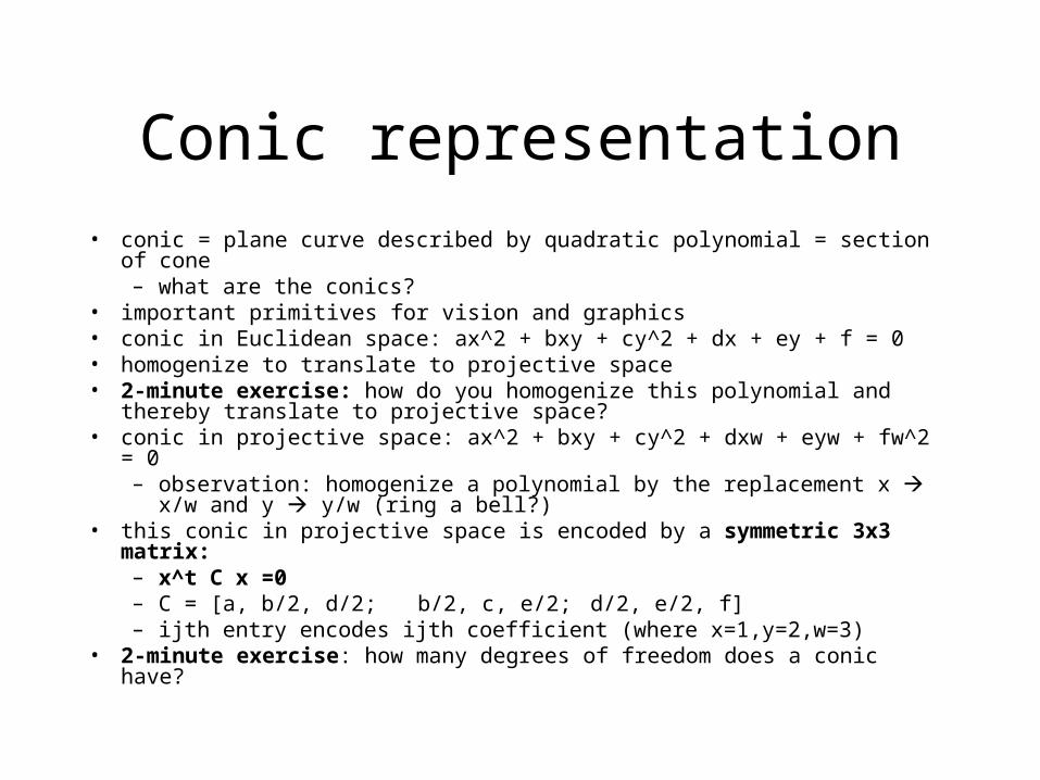
Conic representation

• conic = plane curve described by quadratic polynomial = section of cone– what are the conics?

• important primitives for vision and graphics• conic in Euclidean space: ax^2 + bxy + cy^2 + dx + ey + f = 0• homogenize to translate to projective space • 2-minute exercise: how do you homogenize this polynomial and thereby

translate to projective space?• conic in projective space: ax^2 + bxy + cy^2 + dxw + eyw + fw^2 = 0

– observation: homogenize a polynomial by the replacement x x/w and y y/w (ring a bell?)

• this conic in projective space is encoded by a symmetric 3x3 matrix:– x^t C x =0– C = [a, b/2, d/2; b/2, c, e/2; d/2, e/2, f]– ijth entry encodes ijth coefficient (where x=1,y=2,w=3)

• 2-minute exercise: how many degrees of freedom does a conic have?

Conic representation 2

• matrix C is projective (only defined up to a multiple)• conic has 5dof: ratios {a:b:c:d:e:f} or 6 matrix entries of C

minus scale– kC represents the same conic as C (equivalent to multiplying equation

by a constant)

• in P^2, all conics are equivalent– that is, can transform from a conic to any other conic using projective

transforms– not true in Euclidean space: cannot transform from ellipse to parabola

using linear transformation

• transformation rule: – if point x Hx, then conic C (H-1)^t C H-1

• HZ30-31, 37

Conic tangents

• another calculation is made simple in projective space (and reduces to matrix computation)

• Result: The tangent of the conic C at the point x is Cx.• Proof:

– this line passes through x since x^t Cx = 0 (x lies on the conic)– Cx does not contain any other point y of C, otherwise the entire line

between x and y would lie on the conic: • if y^t C y = 0 (y lies on conic) and x^t C y = 0 (Cx contains y), then

x+\alpha y (the entire line between x and y) also lies on C– thus, Cx is the tangent through x (a tangent is a line with only one

point of contact with conic)

• HZ31

Metric rectification with circular points

DLT algHZ 4.1

Rectification

HZ 2.7

Hierarchy of maps

InvariantsHZ 2.4

Projectivetransform

HZ 2.3

Behaviourat infinity

Primitivespt/line/conic

HZ 2.2

Material for metric rectification

• circular points (34)• similarity iff fixed circular points (52)• conic (55)• dual conic• degenerate conic• C*

∞: conic dual to circular points (or just dual conic)• angle from dual conic• image of dual conic under homography• then we’re ready for the algorithm of Example 2.26 HZ

Line conic• we have considered point conic• points are dual to lines: let’s dualize• suppose conic is nondegenerate (not 2

lines or repeated line), so C is nonsingular• 3x3 matrix C encodes the points of a

conic – x^t C x = 0 if x lies on conic

• matrix C-1 encodes the tangent lines of that conic:

– L is a tangent line of the conic iff • L^t C-1 L = 0

– proof: tangent L = Cx for some point x on conic; x^t C x = 0 so substituting x = C-1L yields (C-1L)^t C (C-1L) = L^t C-1L = 0 (recall that C is symmetric)

• called a dual conic or line conic; conic envelope

• transformation rule: if point x Hx, then dual conic C* H C* H^t

• HZ31,37

Degenerate conics

• there are degenerate point conics and degenerate line conics

• recall the outer product• if L and M are lines, LM^t + ML^t is the

degenerate point conic consisting of these two lines– notice that the matrix is singular (rank 2)

• if p and q are points, pq^t + qp^t is the degenerate line conic consisting of all lines through p or q– [2 pencils of lines, drawing]– notice that this is a line conic (or dual conic)

‘The’ dual conic C*∞

• two circular points I and J• make a degenerate line conic out of them• C*

∞ = IJ^t + JI^t = (1,0,0; 0,1,0; 0,0,0)– all lines through the circular points

• C*∞ will be called ‘the’ dual conic

– although it is the line conic dual to the circular points

• like circular points, C*∞ is fixed under a projective transform iff

it is a similarity• interesting fact: null vector of C*

∞ = line at infinity

• HZ 52-54• explore relationship to angle

Computing angle from C*∞

• how can we measure angle in a photograph?• angle is typically measured using dot product• but dot product is not invariant under homography• consider two lines L and M in projective space (viewed as conventional columns,

not correct rows)• L^t M is replaced by a normalized L^t C*

∞ M– (L^t C*

∞ M) / \sqrt( (L^t C*∞ L) (M^t C*

∞ M))• this is invariant to homography• note that L^t C*

∞ M is equivalent to dot product in the original space– (a1,a2,1) C*

∞ (b1,b2,1) = a1b1 + a2b2• Result: (L^t C*

∞ M) / \sqrt( (L^t C*∞ L) (M^t C*

∞ M)) is the appropriate measure of angle in projective space.

• since angle = arccos (A.B), this is of course a measure of cos(angle), not angle• corollary: angle can be measured once C*

∞ is known• HZ54-55

How C*∞ transforms

• we want to understand how C*∞ transforms under a homography (since we don’t want it to

transform!)• a homography matrix can be decomposed into a projective, affine, and similarity component:

– H = [I 0] [K 0] [sR t] [v^t 1] [0 1] [0 1] = Hp Ha Hs

– note that K is the affine component• recall that line conics transform by C* H C* H^t, so • C*

∞ (Hp Ha Hs) C*∞ (Hp Ha Hs)t

• but the dual conic is fixed under a similarity, so:• C*

∞ (Hp Ha) C*∞ (Hp Ha)t

• which reduces as follows using C*∞ = diag(1,1,0):

• image of C*∞= [KK^t KK^t v ]

• [v^t KK^t v^t KK^t v ]• when line at infinity is not moving, v = 0:• image of C*

∞ in an affinely rectified image = [KK^t 0] [0 0]

• [HZ43 for this decomposition chain of a homography, HZ55]

Metric rectification algorithm

• “We have the technology. We can rebuild him!”

• input: 2 orthogonal line pairs• assume that the image has already been

affinely rectified (i.e., line at infinity is in correct position)

• we are within an affinity of a similarity!• what is this affinity K? use the known

orthogonality (known angle) to solve for K• let S = KK^t: we actually solve for S, then

retrieve K using Cholesky decomposition– note: S has 2 dof (symmetric 2x2)– use the two line angle constraints to solve

for these dof

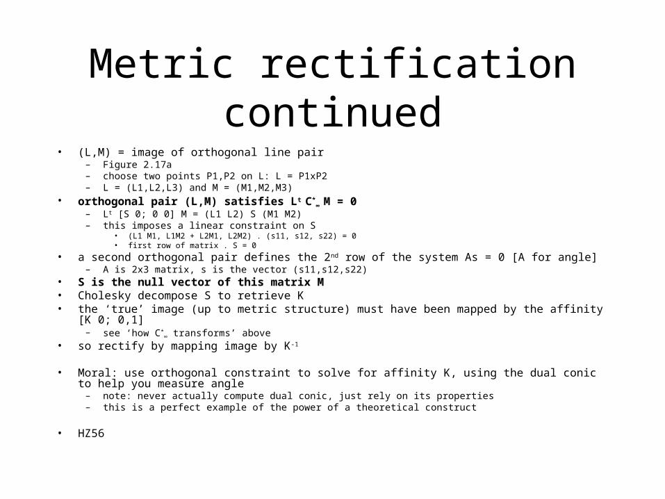
Metric rectification continued• (L,M) = image of orthogonal line pair

– Figure 2.17a– choose two points P1,P2 on L: L = P1xP2– L = (L1,L2,L3) and M = (M1,M2,M3)

• orthogonal pair (L,M) satisfies Lt C*∞ M = 0

– Lt [S 0; 0 0] M = (L1 L2) S (M1 M2)– this imposes a linear constraint on S

• (L1 M1, L1M2 + L2M1, L2M2) . (s11, s12, s22) = 0• first row of matrix . S = 0

• a second orthogonal pair defines the 2nd row of the system As = 0 [A for angle]– A is 2x3 matrix, s is the vector (s11,s12,s22)

• S is the null vector of this matrix M• Cholesky decompose S to retrieve K• the ‘true’ image (up to metric structure) must have been mapped by the affinity [K 0; 0,1]

– see ‘how C*∞ transforms’ above

• so rectify by mapping image by K-1

• Moral: use orthogonal constraint to solve for affinity K, using the dual conic to help you measure angle – note: never actually compute dual conic, just rely on its properties– this is a perfect example of the power of a theoretical construct

• HZ56

Synopsis

• want affinity K

• want S = KK^t

• S is available from the image of C*∞

• get at image of C*∞ using angle relationship

• use orthogonal pairs to solve for image of C*∞

• back out from image of C*∞ to S to K

Numerical aside: solving for null space

• to solve Ax = 0:

1. compute SVD of A = U D V^t

2. if null space is 1d, x = last column of V (called null vector)

3. in general, last d columns of V span the d-dimensional null space

Numerical aside: SVD

• singular value decomposition of A is A = U D V^t, where– mxn A – mxm orthogonal U– mxn diagonal D (containing singular values

sorted)– nxn orthogonal V

• do not compute yourself!• compute using CLAPACK or OpenCV

Other methods for metric rectification

• the 2-ortho-pair method is called stratified rectification• stratification = 2 step approach to removal of distortion, first projective, then affine

• Note: 2 orthogonal lines are conjugate with respect to the dual conic C*∞

• can also rectify (in a stratified fashion) using an imaged circle• image of circle is ellipse: intersect it with vanishing line to find imaged circular points

• can also rectify using 5 orthogonal line pairs– why would you want to? because it doesn’t assume image has already been affinely rectified

• method (your responsibility to read)– find the dual conic as the null vector of a 5x6 matrix built up from 5 linear equations– see DLT algorithm below for a similar approach (this is a very popular approach!)– note: solving for entire 5dof conic, not just the 2dof affine component

• HZ56-57

On OpenCV

• review openCVInstallationNotes• OpenCV demo programs at my website

– cvdemo, cvmousedemo, cvresizedemo, cvpixeldemo

• opencvlibrary.sourceforge.net– invaluable resource for full documentation, FAQ, examples, Wiki

• IPL = Image Processing Library• depth = # of bits in each data value of image

– 8 = uchar, 32 = float

• channels = # of data values for each image pixel– 1 = grayscale; 3 = RGB

Capturing images as test data

• I would like you to personalize your test data• I would also like to gather an image database• assignment: find images replete with parallel lines (and optimally,

vanishing lines inside the image) and orthogonal lines– also want different directions of parallel and orthogonal lines: e.g., brick

wall is not as useful since all parallel lines yield only two distinct ideal points

• challenge: rectification without gaps• challenge: rectification to within a translation using external cues• challenge: rectification from other constraints (e.g., in a natural scene

with no visible lines or circles)• challenge: image contexts with circles and other known nonlinear

curves