Embed Size (px)
Citation preview


Concrete Design to EN 1992
Concrete Design toEN 1992
L.H. Martin Bsc, PhD, CEng FICEJ.A. Purkiss Bsc (Eng), PhD
AMSTERDAM � BOSTON � HEIDELBERG � LONDONNEW YORK � OXFORD � PARIS � SAN DIEGO
SAN FRANCISCO � SINGAPORE � SYDNEY � TOKYO
Butterworth-Heinemann is an imprint of Elsevier

Butterworth-Heinemann
An imprint of Elsevier
Linacre House, Jordan Hill, Oxford OX2 8DP, UK
84 Theobald’s Road, London WC1X 8RR, UK
First published in Great Britain by Arnold 1996
Reprinted by Butterworth-Heinemann 2000
Second Edition 2006
Copyright � 2006, L.H. Martin and J.A. Purkiss. All rights reserved
Permission to reproduce extracts from the BS EN 1997-1:2004 and
BS EN 1991-1-1:2004 is granted by BSI.
The right of L.H. Martin and J.A. Purkiss to be identified as the authors of this Work
has been asserted in accordance with the Copyright, Designs and Patents Act 1988
No part of this publication may be reproduced, stored in a retrieval system or
transmitted in any form or by any means electronic, mechanical, photocopying,
recording or otherwise without the prior written permission of the publisher
Permission may be sought directly from Elsevier’s Science & Technology
Rights Department in Oxford, UK: phone: (þ44) (0) 1865 843830;
fax (þ44) (0) 1865 853333; email: [email protected].
Alternatively you can submit your request online by visiting the Elsevier web site at
http://elsevier.com/locate/permissions, and selecting Obtaining permission to use Elsevier material
Notice
No responsibility is assumed by the publisher for any injury and/or damage to persons
or property as a matter of products liability, negligence or otherwise, or from any use or
operation of any methods, products, instructions or ideas contained in the material
herein. Because of rapid advances in the medical sciences, in particular, independent
verification of diagnoses and drug dosages should be made
British Library Cataloguing in Publication Data
A catalogue record for this book is available from the British Library
Library of Congress Cataloging in Publication Data
A catalogue record for this book is available from the Library of Congress
ISBN 13: 978-0-75-065059-5
ISBN 10: 0-75-065059-1
For information on all Butterworth-Heinemann
publications visit our website at http://books.elsevier.com
Typeset by CEPHA Imaging Pvt. Ltd, Bangalore, India
Printed and bound in Great Britain
06 07 08 09 10 9 8 7 6 5 4 3 2 1

Contents
Preface ix
Acknowledgements xi
Principal Symbols xiii
CHAPTER
1 General 1
1.1 Description of concrete structures 1
1.2 Development and manufacture of reinforced concrete 3
1.3 Development and manufacture of steel 5
1.4 Structural design 6
1.5 Production of reinforced concrete structures 11
1.6 Site conditions 16
CHAPTER
2 Mechanical Properties of Reinforced Concrete 18
2.1 Variation of material properties 18
2.2 Characteristic strength 18
2.3 Design strength 20
2.4 Stress–strain relationship for steel 21
2.5 Stress–strain relationship for concrete 23
2.6 Other important material properties 24
2.7 Testing of reinforced concrete materials and structures 30
CHAPTER
3 Actions 32
3.1 Introduction 32
3.2 Actions varying in time 32
3.3 Actions with spatial variation 34
3.4 Design envelopes 35
3.5 Other actions 37
CHAPTER
4 Analysis of the Structure 39
4.1 General philosophy for analysis of the structure 39
4.2 Behaviour under accidental effects 40
4.3 Frame imperfections 46
4.4 Frame classification 48
4.5 Frame analysis 50
4.6 Column loads 55
4.7 Redistribution 55
4.8 Plastic analysis 62
CHAPTER
5 Durability, Serviceability and Fire 65
5.1 Mechanisms causing loss of durability 65
5.2 Serviceability limit states 70
5.3 Fire 93
CHAPTER
6 Reinforced Concrete Beams in Flexure 105
6.1 Behaviour of beams in flexure 107
6.2 Singly reinforced sections 109
6.3 Doubly reinforced sections 115
6.4 Flanged beams 119
6.5 High strength concrete 127
6.6 Design notes 131
6.7 Effective spans 132
CHAPTER
7 Shear and Torsion 133
7.1 Shear resistance of reinforced concrete 133
7.2 Members not requiring shear reinforcement 135
7.3 Members requiring shear reinforcement 137
7.4 Shear resistance of solid slabs 151
7.5 Shear resistance of prestressed concrete beams 164
7.6 Torsional resistance of reinforced and prestressed concrete 168
vi � Contents
CHAPTER
8 Anchorage, Curtailment and Member Connections 176
8.1 Anchorage 176
8.2 Bar splices 179
8.3 Curtailment of reinforcing bars 181
8.4 Member connections 184
CHAPTER
9 Reinforced Concrete Columns 198
9.1 General description 198
9.2 Theory for axially loaded short columns 199
9.3 Theory for a column subject to an axial load and bending moment
about one axis 200
9.4 Theory for columns subject to axial load and biaxial bending 201
9.5 Types of forces acting on a column 202
9.6 Basic theory for second order forces from buckling 203
9.7 Summary of the design method for columns subject to axial
load and bending 206
CHAPTER
10 Reinforced Concrete Slabs 215
10.1 Types of slab 215
10.2 Design philosophies 216
10.3 Plastic methods of analysis 217
10.4 Johansen yield line method 218
10.5 Hillerborg strip method 246
10.6 Slab design and detailing 249
10.7 Beam and slab assemblies 258
10.8 Flat slabs 265
10.9 Waffle slabs 267
CHAPTER
11 Foundations and Retaining Walls 269
11.1 Types of foundation 269
11.2 Basis of design 271
11.3 Bearing pressures under foundations 274
11.4 Calculation of internal stress resultants in pad foundations 279
Contents � vii

11.5 Pile caps 281
11.6 Retaining walls 286
CHAPTER
12 Prestressed Concrete 321
12.1 Bending resistance of prestressed concrete members at ultimate load 321
12.2 Bending resistance of a prestressed concrete beam at service load 327
12.3 Loss of prestress 340
12.4 Anchorage of tendons 348
ANNEX 357
INDEX 373
viii � Contents

Preface
This book conforms with the latest recommendations for the design of reinforced
and prestressed concrete structures as described in Eurocode 2: Design of Concrete
Structures – Part 1-1: General rules and rules for buildings. References to relevant
clauses of the Code are given where appropriate.
Where necessary the process of design has been aided by the production of
design charts.
Whilst it has not been assumed that the reader has a knowledge of structural
design, a knowledge of structural mechanics and stress analysis is a prerequisite. The
book contains detailed explanations of the principles underlying concrete design and
provides references to research where appropriate.
The text should prove useful to students reading for engineering degrees at
University especially for design projects. It will also aid designers who require an
introduction to the new EuroCode.
For those familiar with current practice, the major changes are:
(1) Calculations may be more extensive and complex.
(2) Design values of steel stresses are increased.
(3) High strength concrete is encompassed by the Eurocode by modifications to the
flexural stress block.
(4) There is no component from the concrete when designing shear links for beams.
This is not the case for slabs where there is a concrete component.
(5) Bond resistance is more complex.
(6) Calculations for column design are more complicated.
(7) For fire performance, the distance from the exposed face to the centroid of the
bar (axis distance) is specified rather than the cover.
NOTE: As this text has been produced before the availability of the National Annex
which will amend, if felt appropriate, any Nationally Determined Parameters, the
recommended values of such parameters have been used. The one exception is
the value of the coefficient �cc allowing for long term effects has been taken as 0,85
(the traditional UK value) rather than the recommended value of 1,0.

Acknowledgements
We would like to thank the British Standards Institute for permission to reproduce
extracts from BS EN 1997-1:2004 and BS EN 1991-1-1:2004. British Standards
can be obtained from BSI Customer Services, 389 Chiswick High Road, London
W4 4AL. Tel: +44(0) 208996 9001. email: [email protected]
BSI Ref Book Ref
EN 1997-1 Tables A1/A3 Table 11.1Table A4 Table 11.2Table A13 Table 11.3
EN 1991-1-1 Table 3.1 Annex ATable 7.4N Table 5.2Table 4.1 Table 5.1Fig 5.3 Fig 6.10Fig 9.13 Fig 11.6Fig 9.9 Fig 11.3

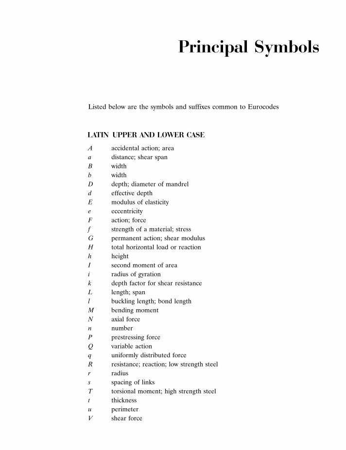
Principal Symbols
Listed below are the symbols and suffixes common to Eurocodes
LATIN UPPER AND LOWER CASE
A accidental action; area
a distance; shear span
B width
b width
D depth; diameter of mandrel
d effective depth
E modulus of elasticity
e eccentricity
F action; force
f strength of a material; stress
G permanent action; shear modulus
H total horizontal load or reaction
h height
I second moment of area
i radius of gyration
k depth factor for shear resistance
L length; span
l buckling length; bond length
M bending moment
N axial force
n number
P prestressing force
Q variable action
q uniformly distributed force
R resistance; reaction; low strength steel
r radius
s spacing of links
T torsional moment; high strength steel
t thickness
u perimeter
V shear force
v shear stress
x neutral axis depth
W load
w load per unit length
Z section modulus
z lever arm
GREEK LOWER CASE
� coefficient of linear thermal expansion; angle of link; ratio; bond factor
� angle; ratio; factor
� partial safety factor
@ deflection; deformation
" strain
� strength factor
� angle of compression strut; slope
� slenderness ratio; ratio
� coefficient of friction
� strength reduction factor for concrete
unit mass; reinforcement ratio
normal stress; standard deviation
� shear stress
� rotation; slope; ratio; diameter of a reinforcing bar; creep coefficient
’ factors defining representative values of variable actions
SUFFIXES
b bond
c concrete
d design value
ef effective
f flange
i initial
k characteristic
l longitudinal
lim limit
m mean
max maximum
min minimum
o original
p prestress
xiv � Principal Symbols

R resistance
req required
s steel
sw self weight
t time; tensile; transfer
u ultimate
v shear
w web; wires; shear reinforcement
y yield
x, y, z axes
Principal Symbols � xv

C h a p t e r 1 / General
1.1 DESCRIPTION OF CONCRETE STRUCTURES1.1.1 Types of Load Bearing Concrete Structures
The development of reinforced concrete, circa 1900, provided an additional building
material to stone, brick, timber, wrought iron and cast iron. The advantages of
reinforced concrete are cheapness of aggregates, flexibility of form, durability and
low maintenance. A disadvantage is greater self weight as compared with steel,
timber or aluminium.
Reinforced concrete structures include low rise and high rise buildings, bridges,
towers, floors, foundations etc. The structures are essentially composed of load
bearing frames and members which resist the actions imposed on the structure,
e.g. self weight, dead loads and external imposed loads (wind, snow, traffic etc.).
Structures with load bearing frames may be classified as:
(a) Miscellaneous isolated simple structural elements, e.g. beams and columns
or simple groups of elements, e.g. floors.
(b) Bridgeworks.
(c) Single storey factory units, e.g. portal frames.
(d) Multi-storey units, e.g. tower blocks.
(e) Shear walls, foundations and retaining walls.
Two typical load bearing frames are shown in Fig. 1.1. When subject to lateral
loading, some frames (Fig. 1.1(a)) deflect and are called sway, or unbraced, frames.
Others (Fig. 1.1(b)) however are stiffened, e.g. by a lift shaft and are called
non-sway, or braced, frames. This distinction is important when analysing frames
as shown in Chapters 4 and 9. For analysis purposes, frames are idealized and
shown as a series of centre lines (Fig. 1.1(c)). Elements of a structure are defined
in cl. 5.3.1, EN.

1.1.2 Load Bearing Members
A load bearing frame is composed of load bearing members (or elements) e.g. beams
and columns. Structural elements are required to resist forces and displacements
in a variety of ways, and may act in tension, compression, flexure, shear, torsion,
or in any combination of these forces. The structural behaviour of a reinforced
concrete element depends on the nature of the forces, the length and shape of
the cross section of the member, elastic and plastic properties of the materials,
yield strength of the steel, crushing strength of the concrete and crack widths.
Modes of behaviour of structural elements are considered in detail in the following
chapters.
A particular advantage of reinforced concrete is that a variety of reinforced concrete
sections (Fig. 1.2) can be manufactured to resist combinations of forces (actions).
(a) Sway frame (b) Non-sway frame (c) Idealized frame
FIGURE 1.1 Typical load bearing frames
(a) Lintel (b) Beam (c) Column
(d) ‘T’ beam
(e) Prestressed beams
FIGURE 1.2 Typical reinforced concrete sections
2 � Chapter 1 / General

The optimization of costs in reinforced construction favours the repeated use of
moulds to produce reinforced concrete elements with the same cross sections and
lengths. These members are common for use in floors either reinforced or
prestressed. The particular advantage of precast concrete units is that the concrete is
matured and will take the full loading at erection. The disadvantage, in some
situations, is the difficulty of making connections.
1.1.3 Connections
The structural elements are made to act as a frame by connections. For reinforced
concrete, these are composed of reinforcing bars bent, lapped or welded which
are arranged to resist the forces involved. A connection may be subject to any
combination of axial force, shear force and bending moment in relation to three
perpendicular axes, but for simplicity, where appropriate, the situation is reduced
to forces in one plane. The transfer of forces through the components of a connec-
tion is often complex and Chapter 8 contains explanations, research references
and typical design examples.
There are other types of joints in structures which are not structural connections.
For example, a movement joint is introduced into a structure to take up the free
expansion and contraction that may occur on either side of the joint due to temp-
erature, shrinkage, expansion, creep, settlement, etc. These joints may be detailed to
be watertight but do not generally transmit forces. Detailed recommendations are
given by Alexander and Lawson (1981). A construction joint is introduced because
components are manufactured to a convenient size for transportation and need to
be connected together on site. In some cases these joints transmit forces but in
other situations may only need to be waterproof.
1.2 DEVELOPMENT AND MANUFACTURE OF REINFORCED CONCRETE
1.2.1 Outline of the Development of Reinforced Concrete
Concrete is a mixture of cement, fine aggregate, coarse aggregate and water.
It is thus a relative cheap structural material but it took years to develop the
binding material which is the cement. Modern cement is a mixture of calcareous
(limestone or chalk) and argillaceous (clay) material burnt at a clinkering temp-
erature and ground to a fine powder.
The Romans used lime mortar and added crushed stone or tiles to form a weak
concrete. Lime mortar does not harden under water and the roman solution was to
grind together lime and volcanic ash. This produced pozzolanic cement named after
a village Pozzuoli near Mount Vesuvius.
Concrete Design � 3
The impetus to improve cement was the industrial revolution of the eighteenth
century. John Smeaton, when building Eddystone lighthouse, made experiments
with various mixes of lime, clay and pozzolana. In 1824, a patent was granted
to Joseph Aspin for a cement but he did not specify the proportions of limestone
and clay, nor did he fire it to such a high temperature as modern cement. However
it was used extensively by Brunel in 1828 for the Thames tunnel. Modern cement is
based on the work of Johnson who was granted a patent in 1872. He experimented
with different mixes of clay and chalk, fired at different temperatures and ground
the resulting clinker.
The mass production of cement was made possible by the invention of the rotary
kiln by Crampton in 1877. The control, quality and reliability of the cement
improved over the years and the proportions of fine and coarse aggregate required
for strong durable concrete have been optimized. This lead to the development
of prestressed concrete using high strength concrete. Most reinforced concrete
construction uses timber as shuttering but where members are repeated, e.g. floor
beams, steel is preferred because it is more robust.
Wilkinson in 1854 took out a patent for concrete reinforced with wire rope.
Early investigators were concerned with end anchorage but eventually continuous
bond between the steel and the concrete was considered adequate. Later, round
mild steel bars with end hooks were standardized with a yield strength of approxi-
mately 200 MPa which gradually increased until today 500 MPa is common. From
1855 reinforced concrete research, construction and theory was developed, notably
in Germany, and results were published by Morsch in 1902.
To overcome the problem of cracking at service load, prestressed concrete was
developed by Freyssinet in 1928. Mild steel was not suitable for prestressed concrete
because all the prestress was lost but high strength piano wires (700 MPa) were found
to be suitable. Initially the post-tensioned system was adopted where the concrete
was cast, allowed to mature and the wires, free to move in ducts, were stressed and
anchored at the ends of the member. Later the pretensioned system was developed
where spaced single wires were prestressed between end frames and the concrete
cast round them. When the concrete had matured, the stress was released and the
force transferred to the concrete by bond between the steel and concrete.
1.2.2 Modern Method of Concrete Production
The ingredients of concrete, i.e. water, cement, fine aggregate and coarse aggregate
are mixed to satisfy the requirements of strength, workability, durability and
economy. The water content is the most important factor which influences the
workability of the mix, while the water/cement ratio influences the strength and
durability. The cement paste (water and cement) should fill the voids in the fine
4 � Chapter 1 / General

aggregate and the mortar (water, cement and sand) should fill the voids in the
coarse aggregate. To optimize this process, the aggregates are graded. Further
understanding of the process can be obtained from methods of mix design
(Teychenne et al., 1975).
The cement production is carefully controlled and tested to produce a consistent
product. The ingredients (lime, silica, alumina and iron) are mixed (puddled) and
fed into a rotary kiln in a continuous process to produce a finely ground clinker.
The chemistry of cement is complicated and not fully understood. For practical
purposes the end product is recognized as either ordinary Portland cement or
rapid-hardening Portland cement.
Fine aggregates (sand) are less than 5 mm, while coarse aggregates (crushed
stone) range from 5 to 40 mm depending on the dimensions of the member.
The aggregates are generally excavated from quarries, washed, mixed to form con-
crete and, for large projects, transported to the construction site. For small
projects, the concrete may be mixed on site from stockpiled materials. Some manu-
factured aggregates are available, including light-weight aggregates, but they are
not often used.
1.3 DEVELOPMENT AND MANUFACTURE OF STEEL
Steel was first produced in 1740 but was not available in large quantities until
Bessemer invented the converter in 1856. By 1840, standard shapes in wrought
iron were in regular production. Gradually wrought iron was refined to control
its composition and remove impurities to produce steel. Further information on
the history of steel making can be found in Buchanan (1972); Cossons (1975);
Derry (1960); Pannel (1964) and Rolt (1970).
Currently there are two methods of steel making:
(a) Basic Oxygen Steelmaking (BOS) used for large scale production. Iron ore
is smelted in a blast furnace to produce pig iron. The pig iron is transferred
to a converter where it is blasted with oxygen and impurities are removed
to produce steel. Some scrap metal may be used.
(b) Electric Arc Furnace (EAF) used for small scale production. The method,
uses scrap metal almost entirely which is fed into the furnace and heated by
means of an electrical discharge from carbon electrodes. Little refining is
required.
In both processes carbon, manganese and silicon in particular, are controlled.
Other elements which may affect coldworking, weldability and bendability may
also be limited. BOS steel has lower levels of sulphur, phosphorous and nitrogen
while EAF steel has higher levels of copper, nickel and tin.
Concrete Design � 5
Traditionally steel was cast into ingots but impurities segregated to the top of the
ingot which had to be removed. Ingots have been replaced by a continuous casting
process to produce a water cooled billet. The billet is reheated to a temperature of
approximately 11508C and progressively rolled through a mill to reduce its section.
This process also removes defects, homogenizes the steel and forms ribs to improve
the bond. With the addition of tempering by controlled quenching it is possible to
produce a relatively soft ductile core with a hard surface layer (Cares, 2004).
1.4 STRUCTURAL DESIGN
1.4.1 Initiation of a Design
The demand for a structure originates with the client. The client may be a private
person, private or public firm, local or national government or a nationalized
industry.
In the first stage, preliminary drawings and estimates of costs are produced,
followed by consideration of which structural materials to use, i.e. reinforced
concrete, steel, timber, brickwork, etc. If the structure is a building, an architect
only may be involved at this stage, but if the structure is a bridge or industrial
building then a civil or structural engineer prepares the documents.
If the client is satisfied with the layout and estimated costs then detailed design
calculations, drawings and costs are prepared and incorporated in a legal contract
document. The design documents should be adequate to detail, fabricate and erect
the structure.
The contract document is usually prepared by the consultant engineer and work
is carried out by a contractor who is supervised by the consultant engineer.
However, larger firms, local and national government and nationalized industries,
generally employ their own consultant engineer.
The work is generally carried out by a contractor, but alternatively direct labour
may be used. A further alternative is for the contractor to produce a design and
construct package, where the contractor is responsible for all parts and stages of
the work.
1.4.2 The Object of Structural Design (cl. 2.1 EN, Section 2 EN 1990)
The object of structural design is to produce a structure that will not become
unserviceable or collapse in its lifetime, and which fulfils the requirements of
the client and user at reasonable cost.
6 � Chapter 1 / General

The requirements of the client and user may include the following:
(a) The structure should not collapse locally or overall.
(b) It should not be so flexible that deformations under load are unsightly or
alarming, or cause damage to the internal partitions and fixtures; neither should
any movement due to live loads, such as wind, cause discomfort or alarm to the
occupants/users.
(c) It should not require excessive repair or maintenance due to accidental overload
or because of the action of weather.
(d) In the case of a building, the structure should be sufficiently fire resistant to,
give the occupants time to escape, enable the fire brigade to fight the fire in
safety, and to restrict the spread of fire to adjacent structures.
(e) The working life of the structure should be acceptable (generally varies
between 10 and 120 years).
The designer should be conscious of the costs involved which include:
(a) Initial cost which includes fees, site preparation, cost of materials and
construction.
(b) Maintenance costs, e.g. decoration and structural repair.
(c) Insurance chiefly against fire damage.
(d) Eventual demolition.
It is the responsibility of the structural engineer to design a structure that is safe
and which conforms to the requirements of the local bye-laws and building regu-
lations. Information and methods of design are obtained from Standards and
Codes of Practice and these are ‘‘deemed to satisfy’’ the local bye-laws and building
regulations. In exceptional circumstances, e.g. the use of methods validated by
research or testing, an alternative design may be accepted.
A structural engineer is expected to keep up to date with the latest research infor-
mation. In the event of a collapse or malfunction where it can be shown that
the engineer has failed to reasonably anticipate the cause or action leading to
collapse or has failed to apply properly the information at his disposal, i.e. Codes
of Practice, British Standards, Building Regulations, research or information
supplied by the manufactures, then he may be sued for professional negligence.
Consultants and contractors carry liability insurance to mitigate the effects of
such legal action.
1.4.3 Statistical Basis for Design
When a material such as concrete is manufactured to a specified mean strength, tests
on samples show that the actual strength deviates from the mean strength to a
varying degree depending on how closely the process is controlled and on the
Concrete Design � 7
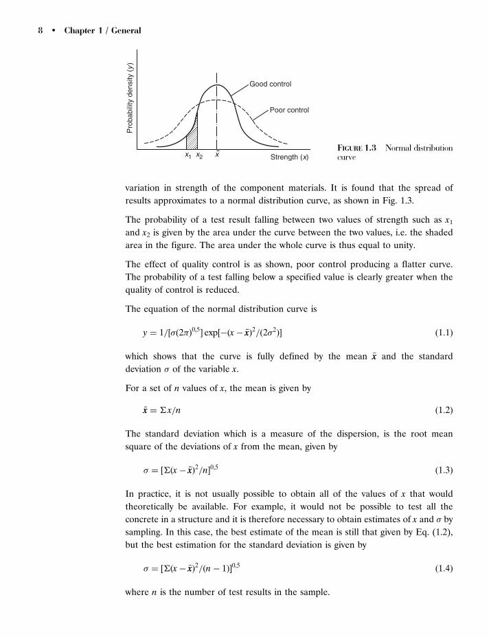
variation in strength of the component materials. It is found that the spread of
results approximates to a normal distribution curve, as shown in Fig. 1.3.
The probability of a test result falling between two values of strength such as x1
and x2 is given by the area under the curve between the two values, i.e. the shaded
area in the figure. The area under the whole curve is thus equal to unity.
The effect of quality control is as shown, poor control producing a flatter curve.
The probability of a test falling below a specified value is clearly greater when the
quality of control is reduced.
The equation of the normal distribution curve is
y ¼ 1=½ð2 Þ0,5� exp½�ðx� �xxÞ2=ð22Þ� ð1:1Þ
which shows that the curve is fully defined by the mean �xx and the standard
deviation of the variable x.
For a set of n values of x, the mean is given by
�xx ¼ � x=n ð1:2Þ
The standard deviation which is a measure of the dispersion, is the root mean
square of the deviations of x from the mean, given by
¼ ½�ðx� �xxÞ2=n�0,5ð1:3Þ
In practice, it is not usually possible to obtain all of the values of x that would
theoretically be available. For example, it would not be possible to test all the
concrete in a structure and it is therefore necessary to obtain estimates of x and by
sampling. In this case, the best estimate of the mean is still that given by Eq. (1.2),
but the best estimation for the standard deviation is given by
¼ ½�ðx� �xxÞ2=ðn� 1Þ�0,5ð1:4Þ
where n is the number of test results in the sample.
Good control
Pro
babi
lity
dens
ity (
y)
Poor control
Strength (x)x1 x2 xFIGURE 1.3 Normal distributioncurve
8 � Chapter 1 / General

For hand calculations, a more convenient form of Eq. (1.4) is
¼ ½ð� x2 � n�xx2Þ=ðn� 1Þ�0,5ð1:5Þ
Statistical distributions can also be obtained to show the variation in strength of
other structural materials such as steel reinforcement and prestressing tendons.
It is also reasonable to presume that if sufficient statistical data were available,
distributions could be defined for the loads carried by a structure. It follows that it
is impossible to predict with certainty that the strength of a structural member will
always be greater than the load applied to it or that failure will not occur in some
other way during the life of the structure. The philosophy of limit state design is to
establish limits, based on statistical data, experimental results and engineering
experience and judgement, that will ensure an acceptably low probability of failure.
At present there is insufficient information to enable distributions of all the
structural variables to be defined and it is unlikely that is will ever be possible to
formulate general rules for the construction of a statistical model of anything so
complicated as an actual structure.
1.4.4 Limit State Design (cl. 2.2 EN)
It is self evident that a structure should be ‘safe’ during its lifetime, i.e. free from
the risk of collapse. There are, however, other risks associated with a structure and
the term safe is now replaced by the term ‘serviceable’. A structure should not
during its lifetime become ‘unserviceable’, i.e. it should be free from risk of collapse,
rapid deterioration, fire, cracking, excessive deflection etc.
Ideally it should be possible to calculate mathematically the risk involved in
structural safety based on the variation in strengths of the material and variation in
the loads. Reports, such as the CIRIA Report 63, have introduced the designer to
elegant and powerful concept of ‘structural reliability’. Methods have been devised
whereby engineering judgement and experience can be combined with statistical
analysis for the rational computation of partial safety factors in codes of practice.
However, in the absence of complete understanding and data concerning aspects of
structural behaviour, absolute values of reliability cannot be determined.
It is not practical, nor is it economically possible, to design a structure that will never
fail. It is always possible that the structure will contain material that is less than the
required strength or that it will be subject to loads greater than the design loads.
It is therefore accepted that 5 per cent of the material in a structure is below
the design strength, and that 5 per cent of the applied loads are greater than
the design loads. This does not mean therefore that collapse is inevitable, because
it is extremely unlikely that the weak material and overloading will combine
simultaneously to produce collapse.
Concrete Design � 9

The philosophy and objectives must be translated into a tangible form using
calculations. A structure should be designed to be safe under all conditions of its
useful life and to ensure that this is accomplished certain distinct performance
requirements, called ‘limit states’, have been identified. The method of limit state
design recognizes the variability of loads, materials construction methods and
approximations in the theory and calculations (BS EN 1990).
Limit states may be at any stage of the life of a structure, or at any stage of loading.
The limit states which are important for the design of reinforced concrete are at
ultimate and serviceability (cl 2.2 EN). Calculations for limit states involve loads
and load factors (Chapter 3), and material factors and strengths (Chapter 2).
Stability, an ultimate limit state, is the ability of a structure or part of a structure, to
resist overturning, overall failure and sway. Calculations should consider the worst
realistic combination of loads at all stages of construction.
All structures, and parts of structures, should be capable of resisting sway forces,
e.g. by the use of bracing, ‘rigid’ joints or shear walls. Sway forces arise from
horizontal loads, e.g. winds, and also from practical imperfections, e.g. lack of
verticality.
Also involved in limit state design is the concept of structural integrity. Essentially
this means that the structure should be tied together as a whole, but if damage
occurs, it should be localized. This was illustrated in a tower block (Canning Town
Report, 1968) when a gas explosion in one flat caused the progressive collapse
of other flats on one corner of the building.
Deflection is a serviceability limit state. Deflections should not impair the efficiency
of a structure or its components, nor cause damage to the finishes. Generally the
worst realistic combination of unfactored imposed loads is used to calculate elastic
deflections. These values are compared with limit states of deformation (cl. 7.4, EN).
Dynamic effects to be considered at the serviceability limit state are vibrations
caused by machines, and oscillations caused by harmonic resonance, e.g. wind gusts
on buildings. The natural frequency of the building should be different from the
exciting source to avoid resonance.
Fortunately there are few structural failures and when they do occur they are often
associated with human error involved in design calculations, or construction, or in
the use of the structure.
1.4.5 Errors
The consequences of an error in structural design can lead to loss of life and damage
to property and it is necessary to appreciate where errors can occur. Small errors in
design calculations can occur in the rounding off of figures but these generally do not
10 � Chapter 1 / General

lead to failures. The common sense advice is that the accuracy of the calculation
should match the accuracy of the values given in the European Code.
Errors that can occur in structural design calculations are:
(1) Ignorance of the physical behaviour of the structure under load which
introduces errors in the basic theoretical assumptions.
(2) Errors in estimating the loads, especially the erection forces.
(3) Numerical errors in the calculations. These should be eliminated by checking,
but when speed is paramount, checks are often ignored.
(4) Ignorance of the significance of certain effects, e.g. creep, fatigue, etc.
(5) Introduction of new materials or methods, which have not been tested.
(6) Insufficient allowance for tolerances or temperature strains.
(7) Insufficient information, e.g. in erection procedures.
Errors that can occur on construction sites are:
(1) Using the wrong number, diameter, cover and spacing of bars.
(2) Using the wrong or poor mix of concrete.
(3) Errors in manufacture, e.g. holes in the wrong position.
Errors that occur in the life of a structure and also affect safety are:
(1) Overloading.
(2) Removal of structural material, e.g. to insert service ducts.
(3) Poor maintenance.
1.5 PRODUCTION OF REINFORCED CONCRETE STRUCTURES1.5.1 Drawings
Detailed design calculations are essential for any reinforced concrete design but
the sizes of the members, dimensions and geometrical arrangement are usually
presented as drawings. The drawings are used by the contractor on site, but if
there are precast units, the drawing for these may be required for a subcontractor.
General arrangement drawings are often drawn to scale of 1:100, while details
are drawn to a scale of 1:20 or 1:10. Special details are drawn to larger scales
where necessary.
Drawing should be easy to read and should not include superfluous detail. Some
important notes are:
(a) Members and components should be identified by logically related mark
numbers, e.g. related to the grid system used in the drawings.
(b) The main members should be presented by a bold outline (0,4 mm wide) and
dimension lines should be unobtrusive (0,1 mm wide).
Concrete Design � 11

(c) Dimensions should be related to centre lines, or from one end; strings of
dimensions should be avoided. Dimensions should appear once only so that
ambiguity cannot arise when revisions occur. Fabricators should not be put in
the position of having to do arithmetic in order to obtain an essential dimension.
(d) Tolerances for erection purposes should be clearly shown.
(e) The grade of steel and concrete to be used should be clearly indicated.
(f) Detailing should take account of possible variations due to fabrication.
(g) Keep the design and construction as simple as possible and avoid changes in
section along the length of a member.
(h) Site access, transport and available cranage should be considered.
Reinforcement drawings are prepared primarily for the steel fixer and should
conform to the standard method of detailing reinforced concrete (Conc. Soc. and
I.S.E report, 1973). The main points to be noted are:
(1) The outline of the concrete should be slightly finer than the reinforcement.
(2) In walls, slabs and columns a series of bars of a particular mark is indicated
by the end bars and only one bar in the series is shown in full; the other bar is
shown as a short line. In Fig. 1.4(a), for example, the reinforcement consists
of two series of bars forming a rectangular grid in plan.
(3) Each series is identified by a code which has the following form: Number,
type, diameter-bar mark-spacing, comment. For example in Fig. 1.4(a) 25T20-
1-250 indicates that the series contains 25 bars in high yields steel (T), 20 mm
diameter, with bar mark 1, spaced at 250 mm between centres. The complete
code is used only once for a particular series and wherever possible should
appear in the plan or elevation of the member. In sections the bars are
identified simply by their bar mark; and again only the end bars need to be
shown.
(4) Since the bars are delivered on site bent to the correct radii, bends do not
need to be detailed and may be drawn as sharp angles.
(5) Dimensions should be in mm rounded to a multiple of 5 mm. There is no
need to write mm on the drawing.
(6) Except with the case of very simple structures the dimensions should refer
only to the reinforcement and should be given when the steel fixer could not
reasonably be expected to locate the reinforcement properly without them.
In many cases, since the bars are supplied to the correct length and shape, no
dimensions are necessary, e.g. Fig. 1.4(a). Dimensions should be given
from some existing reference point, preferably the face of concrete already
been cast. For example, in Fig. 1.4(b) the dimension to the first link is given
from the surface of the kicker, which would have been cast with the floor slab
and is used to locate the column to be constructed. The formwork for the
column is attached to the kicker and the vertical reinforcement starts from the
kicker.
12 � Chapter 1 / General
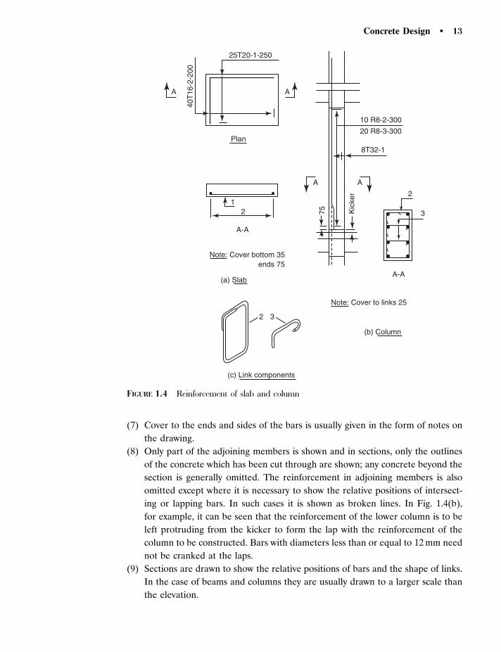
(7) Cover to the ends and sides of the bars is usually given in the form of notes on
the drawing.
(8) Only part of the adjoining members is shown and in sections, only the outlines
of the concrete which has been cut through are shown; any concrete beyond the
section is generally omitted. The reinforcement in adjoining members is also
omitted except where it is necessary to show the relative positions of intersect-
ing or lapping bars. In such cases it is shown as broken lines. In Fig. 1.4(b),
for example, it can be seen that the reinforcement of the lower column is to be
left protruding from the kicker to form the lap with the reinforcement of the
column to be constructed. Bars with diameters less than or equal to 12 mm need
not be cranked at the laps.
(9) Sections are drawn to show the relative positions of bars and the shape of links.
In the case of beams and columns they are usually drawn to a larger scale than
the elevation.
A A
25T20-1-250
10 R8-2-300
20 R8-3-300
8T32-1
A
2
3
A
75 Kic
ker
12
2 3
A-A
Note: Cover bottom 35
Note: Cover to links 25
ends 75
(a) Slab
(b) Column
(c) Link components
A-A
40T
16-2
-200
Plan
FIGURE 1.4 Reinforcement of slab and column
Concrete Design � 13

(10) The ends of overlapping bars in the same plane are shown as ticks.
For example the conventional representation of the links is shown in the
section of the column in Fig. 1.4(b). The actual shapes of the link components
are shown in Fig. 1.4(c). There is no really any need to indicate overlapping
in links except when the separate components are to be fixed on site, as in
this case. Where links are supplied in one piece, as for the beam in Fig. 1.5,
the ticks are frequently omitted.
(11) Section arrows for beams and columns should always be in the same direction,
i.e. left facing for beams, downwards for columns. The section letters (numbers
are not recommended) should always be between the arrows and should be
written in the upright position.
(12) When detailing beams all the bars are shown in full. In elevations, the start
and finish of the bars in the same place are indicated by ticks. The start is
indicated by the full bar code, the end simply by the bar mark (Fig. 1.5)
which shows the elevation and sections of part of a beam. Note that the
reinforcement in the adjoining column and integral floor slab is not shown;
separate drawings would be provided for these. Note also that the dimension
A
A
A-A B-B
Note: Cover to links 25ends 50
1 1 2
5
3 3 3 34 4
5
2
2T25-1
2T25-3
75 6R10-5-150 250 8R10-5-250
2T25-4
2T16-21
B
B
FIGURE 1.5 Reinforcement of a beam
14 � Chapter 1 / General
of the start of the first series of links is given from the face of the column
already constructed and that a dimension is given between each series of links.
(13) Although the reinforcement in adjoining members is not shown, it is important
for the designer to ensure that it will not obstruct the reinforcement of the
detailed member. Thus it is especially important in beam–column construction
to ensure that the reinforcements of a beam and a column do not intersect in
the same plane.
1.5.2 Bar Bending Schedules
Scheduling, dimensioning, bending and cutting of steel reinforcement for concrete is
given in BS 8666 (2000). Bars should be designed to have as few bends as possible
and should conform to the preferred shapes.
Work on the reinforcement, i.e. cutting, bending and fixing in place before the
concrete is placed, is usually dealt with by specialist sub-contractors. Information
on reinforcement is conveyed from the engineer to the sub-contractor by use of a
bar bending schedule, which is a table which provides the following information
about each bar.
Member. A reference identifying a particular structural member, or group of
identical members.
Bar mark. An identifying number which is unique to each bar in the schedule.
Type and size. A code letter: ‘T’ for high yield steel, ‘R’ for mild steel follow-
ing by size of bar in mm, e.g. R16 denotes a mild steel bar 16 mm in diameter.
Number of members. The number of identical members in a group.
Number of bars in each.
Total number.
Length of each bar (mm).
Shape code.
Dimensions required for bending. Five columns specifying the standard dimen-
sions corresponding to the particular shape code. These dimensions contain
allowances for tolerances. If a bar does not conform to one of the preferred
shapes then a dimensioned drawing is supplied.
Bars are delivered to the site in bundles, each of which is labelled with the reference
number of the bar schedule and the bar mark. These two numbers uniquely identify
every bar in the structure.
1.5.3 Tolerances (cl. 4.4.1.3, EN)
Tolerance are limits placed on unintentional inaccuracies that occur in dimension
which must be allowed for in design if structural elements and components are
to resist forces and remain durable.
Concrete Design � 15

The formwork and falsework should be sufficiently stiff to ensure that the tolerance
for the structure, as stipulated by the designer, are satisfied. Tolerance for members
are related to controlling the error in the size of section, and vary from � 5 mm
for a 150 mm section to � 30 mm for a 2500 mm section. Tolerances for position of
prestressing tendons are related to the width of depth of a section.
The tolerances associated with concrete cover to reinforcement are important to
maintain structural integrity and to resistance corrosion. The concrete cover is the
distance between the surface of the reinforcement closest to the nearest concrete
surface. The nominal cover is specified in drawings, which is the minimum cover
cmin (cl 4.4.1.2, EN) plus an allowance for design deviation �cdev (cl 4.4.1.3, EN).
The usual value of �cdev¼ 10 mm.
1.6 SITE CONDITIONS
1.6.1 General
The drawings produced by the structural designer are used by the contractor on site.
Most of the reinforced concrete is cast in situ, on site, and transport and access is
generally no problem, except for the basic materials. Most concrete is ready mix
obtained from specialist suppliers. This avoids having to provide space for storing
cement and aggregates and ensures high quality concrete. Prefabricated products,
e.g. floor beams are delivered by road and erected by crane. Most large sites have a
crane available. On site, the general contractor is responsible for the assembly,
erection, connections, alignment and leveling of the complete structure. During
assembly on site it is inevitable that some components will not fit, despite the
tolerances that have been allowed. The correction of some faults and the consequent
litigation can be expensive.
1.6.2 Construction Rules
To ensure that the structure is constructed as specified by the designers, construction
rules are introduced. For concrete, these cover quality of concrete, formwork,
surface finish, temporary works, removal of formwork and falsework. For steel-
work, the rules cover transport, storage, fabrication, welding, joints and placing.
For prestressed concrete there are additional rules for tensioning, grouting and
sealing.
1.6.3 Quality Control
Quality control is necessary to ensure that the construction work is carried out
to the required standards and rules. Control covers the quality of materials, standard
16 � Chapter 1 / General

of workmanship and the quality of the components. For materials, it includes the
mix of concrete, storage, handling, cutting, welding, prestressing forces and grouting
(BS EN 206-1, 2000).
REFERENCES AND FURTHER READING
Alexander, S.J. and Lawson, R.M. (1981) Movement design in buildings, Technical Note 107,
CIRIA.
BS EN 206-1 (2000) Concrete Pt.1: Specification, performance, production and conformity, BSI.
BS EN 1990 (2002) Eurocode – Basis of structural design.
BS 8666 (2000) Scheduling dimensioning, bending and cutting of steel reinformcement for
concrete, BSI.
Buchanan, R.A. (1972) Industrial Archeology in Britain, Penguin.
Canning Town. Min. of Hous. and Local Gov. (1968) Ronan Point report of the enquiry into the
collapse of flats at Ronan Point.
Cares (2004) Pt.2. Manufacturing process routes for reinforcing steels, UK Cares.
CIRIA Report 63. (1977) Rationalisation of safety and serviceability factors in structural codes.
Conc. Soc. and I.S.E. (1973) Standard methods of detailing reinforced concrete.
Cossons, N. (1975) The BP Book of Industrial Archeology.
Derry, T.K. and Williams, T.I. (1960) A Short History of Technology, Oxford University Press.
Pannel, J.P.M. (1964) An illustrated History of Civil Engineering, Thames and Hudson.
Rolt L.T.C. (1970) Victorian Engineering, Penguin.
Teychenne, D.C., Franklin, R.E. and Erntroy, H.C. (1975) Design of normal concrete mixes,
Dept. of the Env.
Concrete Design � 17

C h a p t e r 2 /Mechanical Properties ofReinforced Concrete
2.1 VARIATION OF MATERIAL PROPERTIES
The properties of manufactured materials vary because the particles of the material
are not uniform and because of inconsistencies in the manufacturing process which
are dependent on the degree of control. These variations must be recognized and
incorporated into the design process.
For reinforced concrete, the material property that is of most importance is strength.
If a number of samples are tested for strength, and the number of specimens with the
same strength (frequency) plotted against the strength, then the results approxi-
mately fit a normal distribution curve (Fig. 2.1). The equation shown in Fig. 2.1
defines the curve mathematically and can be used to define ‘safe’ values for design
purposes.
2.2 CHARACTERISTIC STRENGTH
A strength to be used as a basis for design must be selected from the variation in
values (Fig. 2.1). This strength, when defined, is called the characteristic strength. If
the characteristic strength is defined as the mean strength, then 50 per cent of the
material is below this value and this is unsafe. Ideally the characteristic strength
should include 100 per cent of the samples, but this is impractical because it is a low
value and results in heavy and costly structures. A risk is therefore accepted and it is
therefore recognized that 5 per cent of the samples for strength fall below the
characteristic strength. The characteristic strength is calculated from the equation
fck ¼ fmean � 1,64 ð2:1aÞ
where for n samples the standard deviation
¼ ½�ð fmean � f Þ2=ðn� 1Þ�0,5ð2:1bÞ

2.2.1 Characteristic Strength of Concrete (cl 3.1.2, EN)
Concrete is a composite material which consists of coarse aggregate, fine aggregate
and a binding paste mixture of cement and water. Mix design selects the optimum
proportions of these materials, but a simple way to assess the quality of concrete as it
matures is to crush a standard cube or cylinder.
The mean strength which must be achieved in the mixing process can be determined
if the standard deviation is known from previous experience. For example, to
produce a concrete with a characteristic strength of 30 MPa in a plant for which
a standard deviation of 5 MPa is expected, required mean strength¼ 30þ
5� 1,64¼ 38,2 MPa.
The strength of concrete increases with age and it is necessary to adopt a time after
casting as a standard. The characteristic compressive strength for concrete is the
28-day cylinder or cube strength, i.e. the crushing strength of a standard cylinder, or
cube, cured under standard conditions for 28 days as described in BS EN 12390-1
(2000). The 28-day strength is approximately 80 per cent of the strength at one year,
after which there is very little increase in strength. Strengths higher than the 28-day
strength are not used for design unless there is evidence to justify the higher strength
for a particular concrete.
The characteristic tensile strength of concrete is the uniaxial tensile strength ( fct,ax)
but in practice this value is difficult to obtain and the split cylinder strength ( fct,sp) is
more often used. The relation between the two values is ( fct,ax)¼ 0,9 ( fct,sp). In the
absence of test values of the tensile strength it may be assumed that the mean value
of the tensile strength ( fctm)¼ 0,3( fck)2/3, where fck is the characteristic cylinder
compressive strength. In situations where the tensile strength of concrete is critical,
e.g. shear resistance, the mean value may be unsafe and a 5 per cent fractile
( fctk0,05¼ 0,7 fctm) is used. In other situations where the tensile strength is not
critical, a 95 per cent fractile ( fctk0,95¼ 1,3 fctm) is used. These values are given in
Table 3.1, EN (Annex A2).
BS EN 206-1 (2000) specifies the mix, transportation, sampling and testing of
concrete. Concrete mixes are either prescribed, i.e. specified by mix proportions, or
5% ofresults
Characteristicstrength
Mean strength
Strength
1,64sxx
y
Fre
quen
cy y =s 2π
1e
− 12
2
sx − x
FIGURE 2.1 Variation in materialproperties
Concrete Design � 19

designed, i.e. specified by characteristic strength. For example, Grade C30P denotes
a prescribed mix which would normally give a strength of 30 MPa; Grade C25/30
denotes a designed mix for which a cylinder strength of 25 MPa or cube strength of
30 MPa is guaranteed. The grades recommended by EN are from 12/15 to 50/60 in
steps of approximately 5 MPa for normal weight aggregates. The lowest Grades
recommended for prestressed concrete are C30 for post-tensioning and C40 for
pretensioning.
Although the definition of characteristic strength theoretically allows that a random
test result could have any value, however low, a practical specification for concrete in
accordance with BS EN 206-1 (2000) would require both of the following conditions
for compliance with the characteristic strength, thus excluding very low values:
(a) the average strength determined from any group of four consecutive test results
exceeds the specified characteristic strength by 3 MPa for concretes of Grade
C16/20 and higher, or 2 MPa for concretes of Grade C7,5–C15;
(b) The strength determined from any test result is not less than the specified
characteristic strength minus 3 MPa for concretes of Grade C20 and above, or
2 MPa for concretes of Grade C7,5–C15.
Concrete not complying with the above conditions should be rejected.
2.2.2 Characteristic Strength of Steel (cls 3.2.3 and 3.3.3, EN)
The characteristic axial tensile yield strength of steel reinforcement (fyk) is the yield
stress for hot rolled steel and 0,2 per cent proof stress for steel with no pronounced
yield stress. The value recommended in the European Code is: High yield steel (hot
rolled or cold worked) 500 MPa. For prestressing tendons, the characteristic strength
( fpk), at 0.1 per cent proof stress, varies from 1000 to 2000 MPa depending on the
size of tendon and type of steel.
2.3 DESIGN STRENGTH
The design strength allows for the reduction in strength between the laboratory and
site. Laboratory samples of the material are processed under strictly controlled
standard conditions. Conditions on site vary and in the case of concrete: segregation
can occur while it is being transported; conditions for casting and compaction differ;
there may be contamination by rain; and curing conditions vary especially in hot or
cold weather.
The design strength of a material is therefore lower than the characteristic strength,
and is obtained by dividing the characteristic strength by a partial safety factor (�m).
The value chosen for a partial safety factor depends on the susceptibility of the
20 � Chapter 2 / Mechanical Properties of Reinforced Concrete

material to variation in strength, e.g. steel reinforcement is less affected by site
conditions than concrete.
2.3.1 Design Strength of Steel
The fundamental partial safety factor for steel �s¼ 1,15. For accidental loading,
e.g. exceptional loads, fire or local damage, the value reduces to �s¼ 1,0. For
earthquakes and fatigue conditions values are increased.
2.3.2 Design Strength of Concrete
The fundamental partial safety factor for concrete �c¼ 1,5. For accidental loading,
the value reduces to �c¼ 1,3. For earthquakes and fatigue conditions, values are
increased.
2.4 STRESS–STRAIN RELATIONSHIP FOR STEEL (cl 3.2.7, EN)A shape of the stress–strain curve for steel depends upon the type of steel and the
treatment given to it during manufacture. For reinforcement steel, actual curves for
short term tensile loading have the typical shapes shown in Fig. 2.2. Curves for
compression are similar. See also BS 4449 (1997).
It can be seen (Fig. 2.2) that hot rolled reinforcing steel yields, or becomes
significantly plastic, at stresses well below the failure stress and at strains well below
the limiting strain for concrete (0,0035). In a reinforced concrete member, therefore,
the steel reinforcement may undergo considerable plastic deformation before the
Ultimate Limit State (ULS) is reached, but will not fracture. However large steel
strains are accompanied by the formation of cracks in the concrete in the tensile
zone, and these may become excessive and result in serviceability failure at loads
below the (ULS).
For normal design purposes, the European Code recommends a single, idealized
stress–strain curve (Fig. 2.3) for both hot rolled and cold worked reinforcement.
2.4.1 Modulus of Elasticity for Steel (cl 3.2.7(4), EN)
The modulus of elasticity for steel (Es) is obtained from the linear part of the
relationship between stress and strain (Fig. 2.2). This is a material property and
values from a set of samples vary between 195 and 205 GPa. For design purposes,
this variation is small and the European Code adopts a mean value of Es ¼ 200 GPa.
Concrete Design � 21

The modulus of elasticity for prestressing steel varies with the type of steel from
175 to 195 GPa. Values of the moduli of elasticity are required in calculations
involving deflections, loss of prestress and for the analysis of statically
indeterminate structures.
Prestressing steel
Cold worked steel
Strain
Str
ess
Hot rolledsteel
Es
fyk
f0,2k
f0,ik
euk euk euk
FIGURE 2.2 Typical stress–strain relationships for steel reinforcement
Idealized
Design
Strain
Str
ess
Es
fpk
fyk
fyd = fyk/gs
eud euk
FIGURE 2.3 Design stress–strain relationship for steel reinforcement
22 � Chapter 2 / Mechanical Properties of Reinforced Concrete
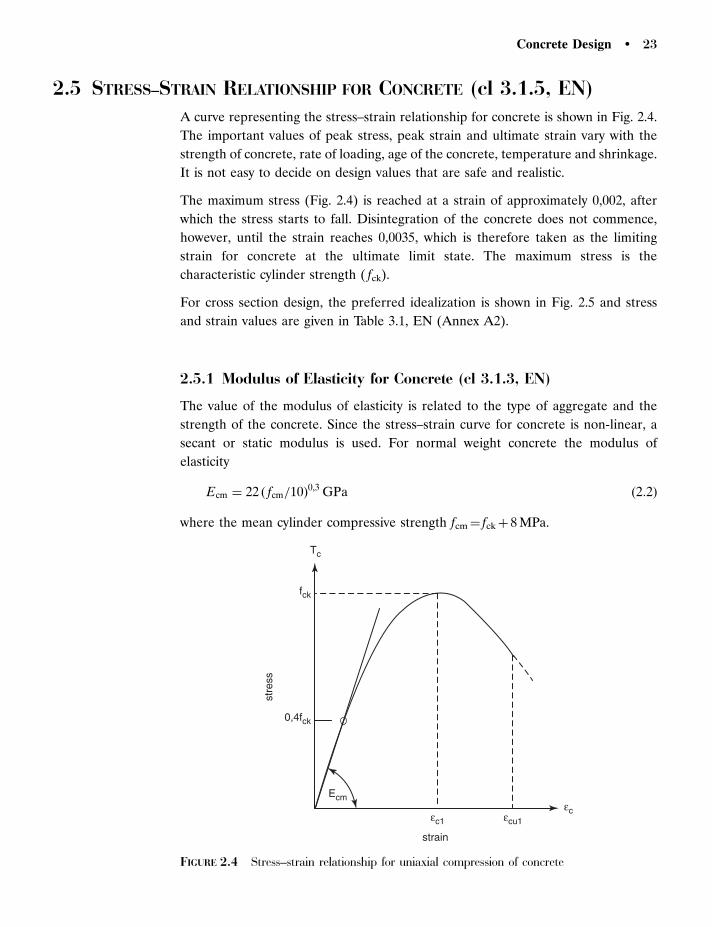
2.5 STRESS–STRAIN RELATIONSHIP FOR CONCRETE (cl 3.1.5, EN)A curve representing the stress–strain relationship for concrete is shown in Fig. 2.4.
The important values of peak stress, peak strain and ultimate strain vary with the
strength of concrete, rate of loading, age of the concrete, temperature and shrinkage.
It is not easy to decide on design values that are safe and realistic.
The maximum stress (Fig. 2.4) is reached at a strain of approximately 0,002, after
which the stress starts to fall. Disintegration of the concrete does not commence,
however, until the strain reaches 0,0035, which is therefore taken as the limiting
strain for concrete at the ultimate limit state. The maximum stress is the
characteristic cylinder strength ( fck).
For cross section design, the preferred idealization is shown in Fig. 2.5 and stress
and strain values are given in Table 3.1, EN (Annex A2).
2.5.1 Modulus of Elasticity for Concrete (cl 3.1.3, EN)
The value of the modulus of elasticity is related to the type of aggregate and the
strength of the concrete. Since the stress–strain curve for concrete is non-linear, a
secant or static modulus is used. For normal weight concrete the modulus of
elasticity
Ecm ¼ 22 ð fcm=10Þ0,3 GPa ð2:2Þ
where the mean cylinder compressive strength fcm¼ fckþ 8 MPa.
Ecm
fck
Tc
0,4fck
εc1 εcu1
εc
strain
stre
ss
FIGURE 2.4 Stress–strain relationship for uniaxial compression of concrete
Concrete Design � 23

Alternatively the modulus of elasticity can be determined from tests, as described in
BS EN 12390 (2000).
2.6 OTHER IMPORTANT MATERIAL PROPERTIES (cl 3.1.3, EN)2.6.1 Introduction
This section gives a brief description of other properties of concrete which affect
design calculations, e.g. deflections and loss of prestress.
2.6.2 Creep (cl 3.1.4, EN)
When a specimen of material is subjected to a stress below the elastic limit,
immediate elastic deformation occurs. In some materials, the initial deformation is
followed, if the load is maintained, by further deformation over a period of time.
This is the phenomena of creep. In concrete, creep is thought to be due to the
internal movement of free or loosely bound water and to the change in shape of
minute voids in the cement paste. The rate of creep varies with time as shown in
Fig. 2.6. Creep affects the deflection of beams at service load and increases the loss
of prestress in prestressed concrete.
It may be assumed that under constant conditions 40 per cent of the total creep
occurs in the first month, 60 per cent in 6 months and 80 per cent in 30 months.
Creep is assumed to be complete in approximately 30 years and is partly recoverable
when the load is reduced. Creep in concrete depends on the following:
(a) composition of the concrete,
(b) original water content,
Compression strain
Idealized
Parabolic axis
Design
fck
fcd
ec2
ec
ec2
sc
ececu2
Com
pres
sion
str
ess
sc = fcd [1− (1− )n] for O ≤ ec ≤ ec2
FIGURE 2.5 Parabolic-rectangular stress–strain relationship for concrete in compression
24 � Chapter 2 / Mechanical Properties of Reinforced Concrete

(c) effective age at transfer of stress,
(d) dimensions of the member,
(e) ambient humidity,
(f) ambient temperature.
For calculation purposes, creep is expressed as a creep coefficient �(�,t0) which
increases the elastic strain to produce the final creep strain, i.e.
"c ¼ elastic strain � coefficient ¼ ðstress=EcmðtÞÞ�ð�,t0Þ ð2:3Þ
where Ecm(t) is the elastic modulus of concrete at age of loading.
Values of the creep coefficient (�(�,t0)) can be calculated from Fig. 3.1, EN. Further
information on creep can be obtained from Annex B, EN and ACI Committee 209
(1972).
2.6.3 Drying Shrinkage (cl 3.1.4, EN)
The total shrinkage strain is composed of;
(a) autogenous shrinkage which occurs during the hardening of concrete,
(b) drying shrinkage which is a function of the migration of water through hardened
concrete.
Drying shrinkage, often referred to simply as shrinkage, is caused by the evaporation
of water from the concrete. Shrinkage can occur before and after the hydration of
the cement is complete. It is most important, however, to minimize it during the
early stages of hydration in order to prevent cracking and to improve the durability
of the concrete. Shrinkage cracks in reinforced concrete are due to the differential
shrinkage between the cement paste, the aggregate and the reinforcement. Its effect
can be reduced by the prolonged curing, which allows the tensile strength of the
concrete to develop before evaporation occurs.
Time30 years
Str
ain
Creep strain
Elastic strain
FIGURE 2.6 Rate of creep
Concrete Design � 25

In prestressed concrete, shrinkage is one of the causes for loss of prestress as
shown in Chapter 12. The most important factors which influence shrinkage in
concrete are:
(a) aggregate used,
(b) original water content,
(c) effective age at transfer of stress,
(d) effective section thickness,
(e) ambient relative humidity,
(f) reinforcement.
2.6.4 Thermal Strains (cl 2.3.1.2, EN)
Thermal effects should be taken into account when checking Serviceability Limit
States (SLS) and at ultimate limit states where significant, e.g. fatigue and second
order effects.
Thermal strains in the concrete are given by
"ct ¼ �ct ð2:4Þ
where
�c is the coefficient of thermal expansion
t is the rise in temperature
Where thermal change is not of much influence, then �c¼ 10E-6/8C. The coefficient
of expansion depends on the type of aggregate and the degree of saturation of the
concrete. Typical values for dry concrete, corresponding to an ambient relative
humidity of 60 per cent, range from 7E-6/8C to 12-6/8C depending on the aggregate.
For saturated and dry concrete, these values can be reduced by approximately
2E-6/8C and 1E-6/8C, respectively.
The thermal coefficient of expansion for steel is �c¼ 12E-6/8C and is used in
calculations for temperature changes which for the UK are in the range of � 58C to
þ 358C. Notice that the coefficients of expansion for steel and concrete are
approximately the same which avoids problems with differential movement.
2.6.5 Fatigue (cls 3.2.6 and 3.3.5 EN)
This is more of a problem with structural steelwork and of lesser importance with
reinforced concrete. However problems may be associated with cracks in high
strength reinforcement at bends, or where welds have been used. Prestressing wires
are also subject to fatigue which should be taken into account.
26 � Chapter 2 / Mechanical Properties of Reinforced Concrete
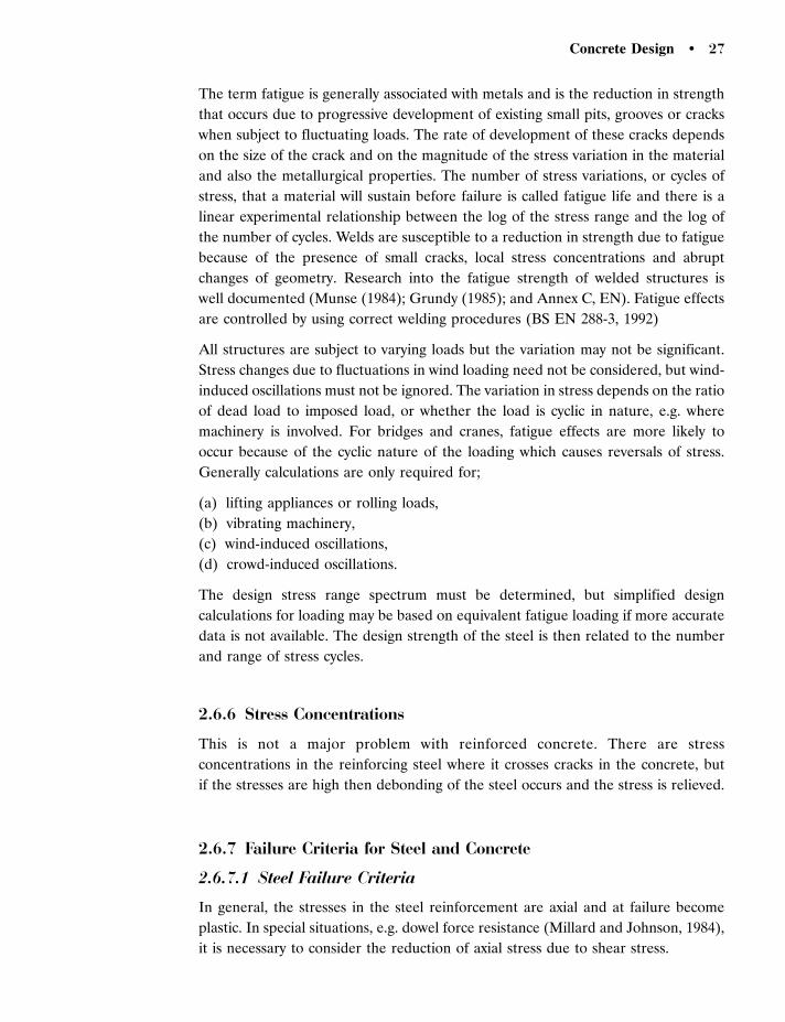
The term fatigue is generally associated with metals and is the reduction in strength
that occurs due to progressive development of existing small pits, grooves or cracks
when subject to fluctuating loads. The rate of development of these cracks depends
on the size of the crack and on the magnitude of the stress variation in the material
and also the metallurgical properties. The number of stress variations, or cycles of
stress, that a material will sustain before failure is called fatigue life and there is a
linear experimental relationship between the log of the stress range and the log of
the number of cycles. Welds are susceptible to a reduction in strength due to fatigue
because of the presence of small cracks, local stress concentrations and abrupt
changes of geometry. Research into the fatigue strength of welded structures is
well documented (Munse (1984); Grundy (1985); and Annex C, EN). Fatigue effects
are controlled by using correct welding procedures (BS EN 288-3, 1992)
All structures are subject to varying loads but the variation may not be significant.
Stress changes due to fluctuations in wind loading need not be considered, but wind-
induced oscillations must not be ignored. The variation in stress depends on the ratio
of dead load to imposed load, or whether the load is cyclic in nature, e.g. where
machinery is involved. For bridges and cranes, fatigue effects are more likely to
occur because of the cyclic nature of the loading which causes reversals of stress.
Generally calculations are only required for;
(a) lifting appliances or rolling loads,
(b) vibrating machinery,
(c) wind-induced oscillations,
(d) crowd-induced oscillations.
The design stress range spectrum must be determined, but simplified design
calculations for loading may be based on equivalent fatigue loading if more accurate
data is not available. The design strength of the steel is then related to the number
and range of stress cycles.
2.6.6 Stress Concentrations
This is not a major problem with reinforced concrete. There are stress
concentrations in the reinforcing steel where it crosses cracks in the concrete, but
if the stresses are high then debonding of the steel occurs and the stress is relieved.
2.6.7 Failure Criteria for Steel and Concrete
2.6.7.1 Steel Failure Criteria
In general, the stresses in the steel reinforcement are axial and at failure become
plastic. In special situations, e.g. dowel force resistance (Millard and Johnson, 1984),
it is necessary to consider the reduction of axial stress due to shear stress.
Concrete Design � 27

The distortion strain energy theory or strain energy theory states that yielding occurs
when the shear strain energy reaches the shear strain energy in simple tension. For a
material subject to principal stresses 1, 2 and 3, this occurs (Timoshenko, 1946)
when
ð1 � 2Þ2þ ð2 � 3Þ
2þ ð3 � 1Þ
2¼ 2f 2
y ð2:5Þ
Alternatively Eq. (2.5) can be expressed in terms of direct stresses b, bc and bt,
and shear stress � on two mutually perpendicular planes. It can be shown from
Mohr’s circle of stress that the principal stresses
1 ¼ ðb þ bcÞ=2 � ½ðb � bcÞ2=4 þ �2�
0,5ð2:6Þ
and
2 ¼ ðb � bcÞ=2 þ ½ðb � bcÞ2=4 þ �2�
0,5ð2:7Þ
If Eqs (2.6) and (2.7) are inserted in Eq. (2.5) with 3¼ 0 and fy is replaced by
the design stress fy/�m then
ð fy=�mÞ2¼ 2
bc þ 2b � bcb þ 3�2 ð2:8Þ
If bc is replaced by bt with a change in sign then
ð fy=�mÞ2¼ 2
bc þ 3�2 ð2:9Þ
2.6.7.2 Concrete Failure Criteria (cl 12.6.3, EN)
Concrete is composed of coarse aggregate, fine aggregate and a cement paste binder.
Since each of these components has variable properties it is not surprising that
concrete is also variable. Concrete includes microcracks in the unloaded state and
when load is applied, the cracks extend and eventually precipitate failure.
The structural behaviour of concrete in tension is brittle and gives little warning of
failure. In compression, behaviour is more plastic with non-linear stress–strain
characteristics and warning signs of failure.
For practical convenience, the quality and strength of concrete is based on the
crushing strength of a cube or cylinder. The value obtained from this test is sensitive
to rate of loading and friction on the patterns. The strength in tension is the uniaxial
tensile strength which is difficult to measure and the split cylinder strength is
specified as an alternative.
Concrete in practice is not often subject to triaxial stresses and generally it is only
necessary to consider biaxial stress conditions. The principal tensile stress failure
28 � Chapter 2 / Mechanical Properties of Reinforced Concrete
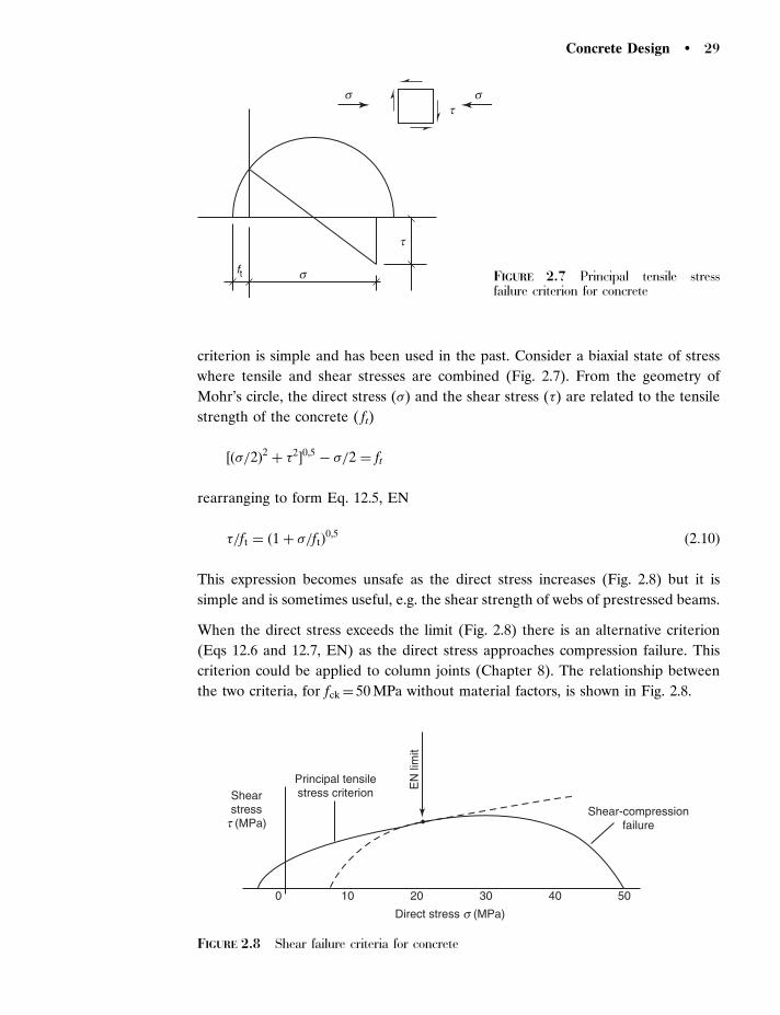
criterion is simple and has been used in the past. Consider a biaxial state of stress
where tensile and shear stresses are combined (Fig. 2.7). From the geometry of
Mohr’s circle, the direct stress () and the shear stress (�) are related to the tensile
strength of the concrete ( ft)
½ð=2Þ2 þ �2�0,5
� =2 ¼ ft
rearranging to form Eq. 12.5, EN
�=ft ¼ ð1 þ =ftÞ0,5
ð2:10Þ
This expression becomes unsafe as the direct stress increases (Fig. 2.8) but it is
simple and is sometimes useful, e.g. the shear strength of webs of prestressed beams.
When the direct stress exceeds the limit (Fig. 2.8) there is an alternative criterion
(Eqs 12.6 and 12.7, EN) as the direct stress approaches compression failure. This
criterion could be applied to column joints (Chapter 8). The relationship between
the two criteria, for fck¼ 50 MPa without material factors, is shown in Fig. 2.8.
s s
sft
t
t
FIGURE 2.7 Principal tensile stressfailure criterion for concrete
0 10 20
Direct stress s (MPa)
30 40 50
Shearstress
t (MPa)
Principal tensilestress criterion
Shear-compressionfailure
EN
lim
it
FIGURE 2.8 Shear failure criteria for concrete
Concrete Design � 29

2.7 TESTING OF REINFORCED CONCRETE MATERIALS
AND STRUCTURES (EN 1990)2.7.1 Testing of Steel Reinforcement
Reinforcing steel is routinely sampled and tested for tensile strength, during
production, to maintain quality. The size, shape, position of the gauges and method
of testing of small sample pieces of steel is given in EN 10002 (2001). The tensile test
gives values of Young’s modulus, limit of proportionality, yield stress or proof stress,
percentage elongation and ultimate stress. Occasionally, when failures occur in
practice, samples of steel are taken from a structure to assess the strength.
Methods of destructive testing fusion welded joints and weld metal in steel are
given in BS EN 288-3 (1992). Welds of vital importance should be subject to non-
destructive tests. The defects that can occur in welds are; slag inclusions, porosity,
lack of penetration and sidewall fusion, liquation, solidification, hydrogen cracking,
lamellar tearing and brittle fracture.
2.7.2 Testing of Hardened Concrete
Concrete supplied, or mixed on a site, is routinely tested by crushing standard cubes
or cylinders when they have hardened. The method of manufacture and testing of
the specimens is laid down in BS EN 12390-1 (2000). Occasionally some of the
cylinders are split to provide the tensile strength of concrete. Rarely, after a
structure is complete, doubt may be cast on the strength of the concrete. Cores can
be cut from the concrete and tested as cylinders but this is expensive and may not be
practical (EN 12504-1, 1999).
Alternatively, non-destructive tests may be used e.g. ultrasonic pulse velocity method
(EN 12504-4, 1998). This consists in passing ultrasonic pulses through concrete from
a transmitting transducer to a receiving transducer. Velocities range from 3 to 5 km/s
and the higher the velocity, higher the strength of concrete. An alternative is the
rebound hardness test (EN 12504-2, 1999) where the amount of rebound increases
with the strength of concrete. This test is not so accurate but gives a rapid assessment
before other methods are considered. The ultrasonic test is the more reliable and
gives information over the thickness of the specimen whereas the rebound test give
only surface values. Further details are given in Neville (1995).
2.7.3 Testing of Structures (EN 1990, Annex D)
Occasionally, new methods of construction are suggested and there may be some
doubt as to the validity of the assumptions of behaviour of the structure. Alterna-
tively if the structure collapses, there may be some dispute as to the strength of a
30 � Chapter 2 / Mechanical Properties of Reinforced Concrete

component, or member, of the structure. In such cases, testing of components, or
part of the structure, may be necessary. However it is generally expensive because of
the accuracy required, cost of material, cost of fabrication, necessity to repeat tests to
allow for variations and to report accurately. Tests are described as;
(a) acceptance tests – non-destructive for confirming structural performance,
(b) strength tests – used to confirm the calculated capacity of a component or
structure,
(c) tests to failure – to determine the real mode of failure and the true capacity
of a specimen,
(d) check tests – where the component assembly is designed on the basis of tests.
Structures which are unconventional, and/or methods of design which are unusual or
not fully validated by research, should be subject to acceptance tests. Essentially,
these consist of loading the structure to ensure that it has adequate strength to
support, e.g.
1,0 ðtest dead load) þ 1,15 ðremainder of dead load) þ 1,25 ðimposed load):
REFERENCES AND FURTHER READING
ACI Committee 209 (1972) Shrinkage and creep in concrete. ACI Bib. No. 10.
BS EN 288-3 (1992) Specification and approval of welding procedures for metallic materials. Welding
procedure tests for the arc welding of steels, BSI.
BS 4449 (1997) Carbon steels for the reinforcement of concrete, BSI.
BS EN 206-1 (2000) Concrete Pt 1. Specification, performance, production and conformity, BSI.
BS EN 12390-1 (2000) Testing hardened concrete, BSI.
EN 12504-1 (1999) Testing concrete in structures- Part 1: Cored specimens – Taking examining and
testing in compression. BSI.
EN 12504-4 (1998) Testing concrete in structures – Part 4: Determination of ultrasonic pulse velocity,
BSI.
EN 12504-2 (1999) Testing concrete in structures – Part 2: Non-destructive testing – determination of
rebound number, BSI.
EN 10002 (2001) Methods of testing of metallic materials, BSI.
EN 1990 (2002) Basis of structural design.
Grundy, P. (1985) Fatigue limit design for steel structures. Civ. Eng. Trans., ICE, Australia, CE27,
No. 1.
Millard, S.G. and Johnson, R.P. (1984) Shear transfer across cracks in reinforced concrete due
to aggregate interlock and dowel action, Mag. Conc. Res., Vol. 36, No 126, March 9–21.
Munse, W.H. (1984) Fatigue of welded structures, Welding Res. Council, New York.
Neville, A.M. (1995) Properties of Concrete, Longman, London.
Timoshenko, S. (1946) Strength of Materials Pt II. Van Nostrand, New York.
Concrete Design � 31
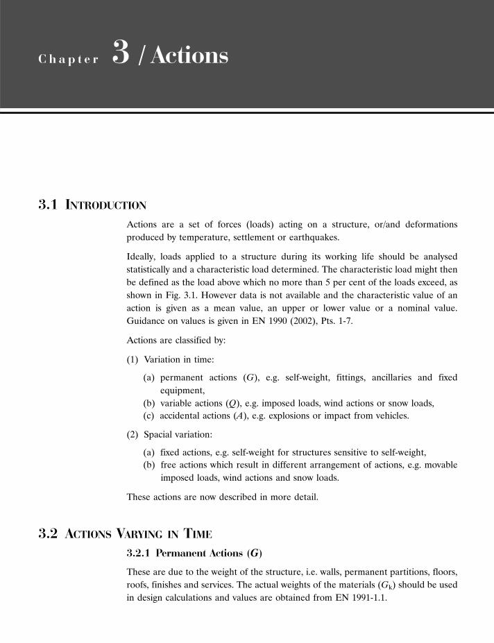
C h a p t e r 3 / Actions
3.1 INTRODUCTIONActions are a set of forces (loads) acting on a structure, or/and deformations
produced by temperature, settlement or earthquakes.
Ideally, loads applied to a structure during its working life should be analysed
statistically and a characteristic load determined. The characteristic load might then
be defined as the load above which no more than 5 per cent of the loads exceed, as
shown in Fig. 3.1. However data is not available and the characteristic value of an
action is given as a mean value, an upper or lower value or a nominal value.
Guidance on values is given in EN 1990 (2002), Pts. 1-7.
Actions are classified by:
(1) Variation in time:
(a) permanent actions (G), e.g. self-weight, fittings, ancillaries and fixed
equipment,
(b) variable actions (Q), e.g. imposed loads, wind actions or snow loads,
(c) accidental actions (A), e.g. explosions or impact from vehicles.
(2) Spacial variation:
(a) fixed actions, e.g. self-weight for structures sensitive to self-weight,
(b) free actions which result in different arrangement of actions, e.g. movable
imposed loads, wind actions and snow loads.
These actions are now described in more detail.
3.2 ACTIONS VARYING IN TIME
3.2.1 Permanent Actions (G)
These are due to the weight of the structure, i.e. walls, permanent partitions, floors,
roofs, finishes and services. The actual weights of the materials (Gk) should be used
in design calculations and values are obtained from EN 1991-1.1.

3.2.2 Variable Actions (Q)
These are due to moveable items such as furniture, occupants, machinery, vehicles,
stored materials, snow and wind. Imposed loads generally are expressed as static
loads for convenience, although there may be minor dynamic forces involved.
Characteristic variable actions (Qk) are subdivided into:
(a) Imposed floor loads are variable actions, and various dwellings values are given
in EN 1991-1.1. These loads include a small allowance for impact and other
dynamic effects that may occur in normal occupancy. They do not include forces
resulting from the acceleration and braking of vehicles or movement of crowds.
The loads are usually given in the form of a distributed load or an alternative
concentrated load. The one that gives the most severe effect is used in design
calculations.
When designing a floor, it is not necessary to consider the concentrated load if
the floor is capable of distributing the load, and for the design of the supporting
beams the distributed load is always used. When it is known that mechanical
stacking of materials is intended, or other abnormal loads are to be applied to
the floor, then actual values of the loads should be used, not those obtained
from EN 1991-1.1. In multi-storey buildings, the probability that all the floors
will simultaneously be required to support the maximum loads is remote and
reductions to column loads are therefore allowed.
(b) Imposed roof loads are variable actions, and are related to snow load and access
for maintenance. They are specified in EN 1991-1.3 and, as with floor loads, they
are expressed as a uniformly distributed load on plan, or as an alternative
concentrated load. The magnitude of the loads decrease as the roof slope
increases and in special situations, where roof shapes are likely to result in
drifting of snow, then loads are increased.
(c) Wind actions are variable but for convenience they are expressed as static
pressures in EN 1991-4. The pressure at any point on a structure is related to the
shape of the building, the basic wind speed, topography and ground roughness.
The effects of vibration, such as resonance in tall buildings must be considered
separately.
Fre
quen
cy
Meanload
1,64s Characteristicload
5% of results
FIGURE 3.1 Variation in load
Concrete Design � 33
3.2.3 Accidental Actions (A)
(a) Dynamic actions (vibration, shock, acceleration, retardation and impact) are
of importance in the design of cranes and information on loads and impact
effects can be obtained from EN 1991-1.7. Vertical static crane loads are
increased by percentages from 10 to 25 per cent depending on whether the
crane is hand or electrically operated. When designing for earthquakes, the
inertial forces must be calculated (EN 1998). This is not of major importance in
the UK.
(b) Accidental actions include explosions and fire as described in Chapter 5.
3.3 ACTIONS WITH SPATIAL VARIATION3.3.1 Pattern Loading (cl 5.1.3, EN)
All possible actions appropriate to a structure should be considered in design
calculations. The actions should be considered separately and in realistic
combinations to determine which is most critical for strength and stability of the
structure.
For continuous structures, connected by rigid joints or continuous over the supports,
vertical actions should be arranged in the most unfavourable but realistic pattern for
each element. Permanent actions need not be varied when considering such pattern
loading, but should be varied when considering stability against overturning. Where
horizontal actions are being considered pattern loading of vertical actions need not
be considered.
For the design of a simply supported beam, it is obvious that the critical condition for
strength is when the beam supports the maximum permanent action and maximum
variable action at the ultimate limit state. The size of the beam is then determined
from this condition and checked for deflection at the serviceability limit state.
A more complicated structure is a simply supported beam with a cantilever as shown
in Fig. 3.2 (a).
Assuming that the beam is of uniform section and that the permanent actions are
uniformly applied over the full length of the beam, it is necessary to consider various
combinations of the variable actions as shown in Figs 3.2 (b)–(d). Although partial
loading of spans is possible, this is not generally considered except in special cases of
rolling actions, e.g. a train on a bridge span.
For a particular section, it is not immediately apparent which combination of actions
is most critical because it depends on the relative span dimensions and magnitude of
the actions. Therefore calculations are necessary to determine the condition and
section for maximum bending moment and shear force at the ULS.
34 � Chapter 3 / Actions
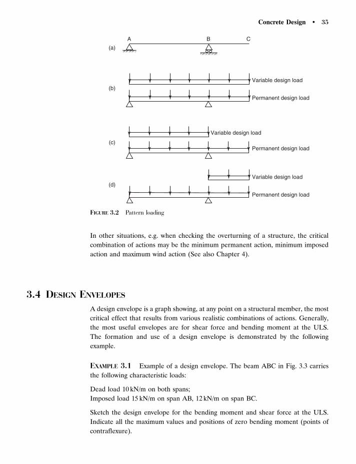
In other situations, e.g. when checking the overturning of a structure, the critical
combination of actions may be the minimum permanent action, minimum imposed
action and maximum wind action (See also Chapter 4).
3.4 DESIGN ENVELOPES
A design envelope is a graph showing, at any point on a structural member, the most
critical effect that results from various realistic combinations of actions. Generally,
the most useful envelopes are for shear force and bending moment at the ULS.
The formation and use of a design envelope is demonstrated by the following
example.
EXAMPLE 3.1 Example of a design envelope. The beam ABC in Fig. 3.3 carries
the following characteristic loads:
Dead load 10 kN/m on both spans;
Imposed load 15 kN/m on span AB, 12 kN/m on span BC.
Sketch the design envelope for the bending moment and shear force at the ULS.
Indicate all the maximum values and positions of zero bending moment (points of
contraflexure).
A
(a)
(b)
(c)
(d)
B C
Variable design load
Variable design load
Variable design load
Permanent design load
Permanent design load
Permanent design load
FIGURE 3.2 Pattern loading
Concrete Design � 35

The maximum and minimum loads on the spans are:
Maximum on AB ¼ 10 � 1,4 þ 15 � 1,6 ¼ 38 kN=m;
Maximum on BC ¼ 10 � 1,4 þ 12 � 1,6 ¼ 33; 2 kN=m;
Maximum on AB or BC ¼ 10 � 1,0 ¼ 10 kN=m:
Consider the following load cases:
(1) Maximum on AB and BC.
(2) Maximum on AB, minimum on BC.
(3) Minimum on AB, maximum on BC.
The bending moment and shear force diagrams are shown in Fig. 3.3.
Comments:
(a) Only the numerical value of the shear force is required in design, the sign
however may be important in the analysis of the structure.
(b) Positive (sagging) bending moments indicate that the bottom of the beam will be
in tension; negative (hogging) moments indicate that the top of the beam will be
in tension. Since the beams will need to be reinforced in the tension zone, it is
conventional to draw the bending moment on the tension side, as shown.
Bending moment (kNm)
109 (2)
0,21m
2,40 m
87,9
6,9
2,34 m
Shear force (kN)
E F20
66,4 (1)(3)
108,3 (1)99,0
38,3
EnvelopeCase 3Case 2Case 1
20,0
(1)(3) 66,4(2) 91,0
81,7
11,7
A B C
FIGURE 3.3 Example: design envelope
36 � Chapter 3 / Actions

(c) The envelope, shown as a heavy line, indicates the maximum values produced by
any of the load cases. Note that on AB the envelope for shear force changes
from case (2) to case (1) at the point where the numerical values of the shear
force are equal.
(d) From the bending moment envelope it is evident that tension reinforcement in
the top of the beam is governed by case (3) and in the bottom of the beam by
case (2). Note that in some regions, tension reinforcement is required in both
the top and the bottom of the beam.
(e) The points of contraflexure indicate theoretical points where the reinforcement
may be curtailed, i.e. at points E and F on the bending moment envelope.
This process is tedious and an experienced designer often knows the critical action
combinations and the positions of the critical values, which avoids some of the
work involved. Alternatively the diagrams can be generated from input data using
computer graphics. In more complicated structures and loading situations, envelopes
are useful in determining where a change of member size could occur and where
splices could be inserted. In other situations, wind action is a further alternative to
combinations of permanent and variable actions.
3.5 OTHER ACTIONS(a) Temperature forces and moments are induced into reinforced concrete
structures which are restrained or highly redundant. Where it is necessary
to allow for temperature change in the UK, the range is usually �58C to þ 358C.
Thermal effects should be taken into account for serviceability limit states
but at ultimate limit states only when significant (cl 2.3.1.2, EN). See also
EN 1991-1.5.
(b) Erection forces may be of importance in reinforced concrete construction where
prefabrication is used. Suspension points for members or parts of structures
may have to be specified to avoid damage to components. It is extremely
difficult to anticipate all possible erection forces and the contractor is
responsible for erection which should be carried out with due care and
attention. Nevertheless a designer should have knowledge of the most likely
method of erection and design accordingly. If necessary temporary stiffening or
supports should be specified, and/or instructions given. See also EN 1991-1.6.
(c) Earth loads occur in situations such as a retaining walls and foundations. Advice
on earth pressures and allowable bearing pressures for different types of soil
at service load conditions is given in EN 1997-1.
(d) Differential settlement is likely to occur in mining areas and values that are
likely to occur in the vicinity of the structure should be determined. Methods of
accommodating the settlement include use of adjustable bearings, pin joints and
adjustable stiffeners.
Concrete Design � 37

REFERENCES AND FURTHER READING
EN - 1991 (2003) Parts 1–7. Actions on structures.
EN - 1990 (2002) Basis of structural design.
EN - 1998 (2006) Designs of structures for earthquake resistance.
38 � Chapter 3 / Actions

C h a p t e r 4 / Analysis of the Structure
Chapter 3 has considered the imposition of structural actions be they loads,
deformations or thermal movements together with the concepts of limit state
design, whether at ultimate (ULS) or serviceability (SLS). This chapter considers
the methods that may be used to determine the internal forces in the structure
due to the actions applied to it.
4.1 GENERAL PHILOSOPHY FOR ANALYSIS OF THE STRUCTURE
The engineer is free to choose the idealization (or model) to represent the structure.
This model must however be realistic, and not be chosen for, say, sheer simplicity.
If in doubt, any model should give a lower bound solution for the internal forces in
all critical elements within the structure. Generally analysis methods will provide
the designer with the internal forces or stress resultants, namely bending moments,
shear forces and axial forces and may provide displacements. Methods which give
internal stresses and strains, such as finite element methods, are not precluded
although care is needed in the interpretation of results. The common mathematical
idealizations of material (and hence element) behaviour are elastic, elastic with
redistribution, plastic (with or without second order effects due to additional
moments induced by large deformations).
4.1.1 Ultimate Limit State
Whatever the method used to determine the internal forces, the actions applied to
the structure must be factored using those values pertaining to ULS, whether for
single or multiple variable loads. Full plastic analysis may not be used for frames
unless the plastic hinges, other than the last one to form, occur in the beams. This is
because columns with high axial loads will not have any ductile capacity (and will not
therefore satisfy the maximum limits for neutral axis depth to effective depth ratios
(x/d) (Section 6.1.1)). This therefore means that frames are normally analysed
elastically and the moment field then adjusted using redistribution to simulate
plastic behaviour.

For slabs, plastic analysis using the Johansen Yield Line methods may be used, but
there are severe restrictions on the x/d ratio to ensure ductility. In practice, however,
due to the relatively low levels of reinforcement, the x/d ratio is rarely critical. It must
be noted the maximum amount of redistribution is reduced and plastic analysis
prohibited if Class A reinforcement is used.
Care needs taking where high membrane forces can be generated, in such as multi-
bay flat slabs, as yield line analysis cannot then be used as again ductility will be
limited. The method may however give valuable insights into the behaviour of flat
slabs around column heads (Regan, 1981 and Oliviera, Regan and Melo, 2004).
In all cases a lower bound approach such as the Hillerborg Strip method can be used
(See Chapter 10).
In elastic analyses, the section properties are generally calculated on the gross
concrete section (with no allowance for the reinforcement), and Young’s modulus
taken as the secant modulus, Ecm (in GPa),
Ecm ¼ 22fck þ 8
10
� �0;3
ð4:1Þ
where fck (MPa) is the concrete grade strength (Table 3.1 of EN 1991-1-2).
4.1.2 Serviceability Analysis
This must be performed using an elastic analysis and contain all actions applied to
the structure including any deformations or settlement effects. It is not generally
necessary to consider time-dependant effects such as creep, except where they will
cause substantial changes in internal forces. This last will occur in hyperstatic
prestressed concrete structures such as continuous bridge decks. Although normal
reinforced concrete undergoes creep, the effect is less as the stress levels are
potentially lower and thus is effectively ignored.
Generally a full serviceability analysis (and design) will be unnecessary. For most
structures, it is sufficient to use ‘deemed to satisfy’ approaches for, say, deflection or
cracking. Exceptions to this approach are where there is an explicit requirement to
determine crack widths in liquid-retaining structures or bridgeworks, or a design
which fails the ‘deemed to satisfy’ clauses, but needs to be shown to be adequate. It is
accepted that ‘deemed to satisfy’ clauses are conservative.
4.2 BEHAVIOUR UNDER ACCIDENTAL EFFECTS
Accidental actions should be considered in a number of possible circumstances:
� Explosions, whether due to gas or terrorism
� Impact due to vehicles or aircraft
40 � Chapter 4 / Analysis of the Structure

Should the risk of such an incident be high and the effects be catastrophic, or in
certain circumstances the need to check be mandatory (e.g. vehicular impact on
bridge piers), then the designer must ensure that the structure is designed and
detailed to ensure that should an accidental situation occur, the structure does not
suffer complete or partial collapse from either the accidental situation itself or
subsequent events such as spread of fire.
Four now classic cases where collapse occurred due to accidental or terrorist
action are:
� Ronan Point block of flats, where a gas explosion blew out a wall panel causing
progressive collapse of a corner of the structure (Wearne, 1999).
� The Alfred P. Murrah Building in Oklahoma City where collapse was caused by a
terrorist bomb blast (Wearne, 1999).
� World Trade Centre Towers in New York on 11 September 2001 due to impact
from deliberate low-flying aircraft and subsequent fire spread. Although the
towers were steel-framed structures, there is still a lesson to be learnt for any form
of construction (ISE, 2002).
� Pentagon Building on 11 September 2001 into which a commercial airline was
crashed. The structure suffered partial but not extensive collapse due to the
impact and subsequent fire (Mlakar et al., 2003).
4.2.1 Progressive Collapse
EN 1990 identifies the need to consider that in the event of an accident such as
explosion or fire, the structure should not exhibit disproportionate damage. This is
reinforced by the requirements of the relevant Building Regulations within the UK,
e.g. the recently revised Approved Document A of the England and Wales Building
Regulations.
Such damage can be mitigated by:
(a) Attempting to reduce or limit the hazard
In the case of fire, this could be done by full consideration given to the use of
non-flammable materials within the structure and by the provision of relevant
active fire protection measures such as sprinklers. In the case of industrial
processes where explosions are a risk then such potential risks need to be taken
into account by, say, enclosing the process in blast-proof enclosures.
(b) Maintenance
The recent Pipers Row Car Park collapse (Wood, 2003) indicates the need for
adequate design, especially where punching shear may be critical as this is a
quasi-brittle failure and the need for adequate inspection and maintenance
where it is known that environmental effects will be severe. Although the failure
Concrete Design � 41

was due to poor maintenance, it was exacerbated by uneven reaction distribution
at the slab–column interface and no tying through the lower face of the slab.
Admittedly the construction technique used would have made the latter
extremely difficult although it contributed to the former.
(c) Consideration of the structural form
A case where this is relevant is when the structure could be subject to externally
provoked explosions. One reason why the damage was extensive following the
Oklahoma City explosion was that the blast was amplified by an overhanging
portion of the structure above ground floor level. A solution for structures
known to be at potential risk is to provide an external curtain which is not
structural and is easily blown out whilst ensuring the structure is stabilized by a
core which is in the centre of the building. Additionally the risk can be mitigated
by ensuring vehicles cannot come within certain limiting distances of the
structure. More information on this including assessment of blast forces is given
in a SCI publication (Yandzio and Gough, 1999) most of which is relevant to
concrete construction.
(d) Removal of key elements to establish stability
In this approach a risk analysis is carried out to identify the key elements in a
structure which are vital for its stability. A structural analysis is carried out with
any one these elements removed to establish the stability of the remaining
structure and its ability to carry the loading so induced. As this is an accidental
limit state, lower partial safety factors are used on both the loading and the
material strengths determining the member strengths. It is not necessary to
check any serviceability limit states.
(e) Ensuring the structure is adequately tied to resist collapse
This needs considering on two levels. The first is to determine the magnitudes of
the likely levels of tying force required. The second is to provide properly
detailed reinforcement to the structure. Such ties are generally peripheral and
vertical. It is permitted to use the reinforcement provided for structural strength
for these and not normally necessary to supply additional reinforcement
unless that needed for normal structural strength is inadequate (cl 9.10.1).
The following system of ties is recommended by EN 1992-1-1:
� Peripheral Ties
Peripheral ties round the external structural envelope (or internal voids)
should be designed to take a force of Ftie,per given by
Ftie,per ¼ Liq1 � q2 ð4:2Þ
where Li is the length of the appropriate span, q1 has a recommended value
of 10 kN/m and q2 of 70 kN.
42 � Chapter 4 / Analysis of the Structure
� Internal Ties
These should be at roof and each floor level, be continuous and effectively
anchored to the peripheral ties. The recommended design force Ftie,int
is 20 kN. In floors without screeds (i.e. where ties cannot be placed in
the span direction), the minimum force on the beam line Ftie should be
taken as
Ftie ¼L1 þ L2
2q3 � q4 ð4:3Þ
where L1 and L2 are the span lengths of the floor slab on either side of
the beam, q3 has a recommended value of 20 kN/m and q4 of 70 kN. It is clear
that where punching shear is a critical failure mode, bottom steel needs
to be continuous through the column to avoid disproportionate collapse
(Reagan, 1981; Wood, 2003).
� Horizontal ties to columns and walls
Edge columns and walls should be tied horizontally at the roof and each floor
level as appropriate. Corner columns should be tied in each direction, but the
reinforcement provided for peripheral ties may also be used for the
horizontal ties. For walls, the recommended value of the tying force Ftie,fac
is 20 kN, and for columns Ftie,col¼ 150 kN.
� Vertical Ties
In panel buildings of 5 storeys or more, vertical ties must be provided to limit
the damage to a floor should the wall or column immediately below be lost.
There is no recommendation made on the actual values of force to be resisted
as each case needs evaluating on an individual basis.
4.2.2 Structure Stability
Any structure with high lateral loading or where vertical loading can be applied
outside the frame envelope must be checked for overturning. Also any continuous
member with a cantilever must be checked for the possibility of uplift on any
support.
In all these cases the loading which causes overturning is deemed to be
unfavourable, and the loading tending to restore the situation is known as
favourable. This is defined in EN 1990 as verification of static equilibrium EQU.
For this situation the partial safety factors given in Table 11.1 (corresponding to
EQU) must be used.
Concrete Design � 43

EXAMPLE 4.1 High wind load. Consider the possibility of overturning for the
water tower shown in Fig. 4.1.
Taking Moments about Point A:
Unfavourable effects due to wind:
1,5 � 120 � ð3 þ 35 þ 1,5Þ þ 1,5 � 6 � 35ð35=2 þ 1,5Þ ¼ 13 095 kNm
Favourable effects due to self weight:
0,9 � 1500 � 14=2 þ 0,9 � 32 � 35 � 14=2 ¼ 16 506 kNm
The moment due to the favourable effects exceeds that due to the unfavourable
effect, thus the structure will not overturn.
EXAMPLE 4.2. External loading. Consider the cantilevering frame shown in
Fig. 4.2.
Here the check is more complex, as the permanent load of 220 kN per storey is
both favourable and unfavourable, in that the load acting on the cantilever is
Wk = 120 kNGK = 1500 kN
gK = 32 kN/m
3 m 6 m
35 m
14 m1.5 mA
wK = 6 kN/m
FIGURE 4.1 Design data forExample 4.1
wk =13 kN/m
7 m 1 mB
5 @3.5 mGK = 220 kN/storey
FIGURE 4.2 Design data for Example 4.2
44 � Chapter 4 / Analysis of the Structure
unfavourable as it contributes to the overturning effect. The permanent load per
storey may be expressed as 27,5 kN/m run.
The favourable part of the permanent loading on the internal span takes a factor
of 0,9, and that on the cantilever of 1,1.
Taking moments about B:
Effect due to the wind loading:
1,5 � 13 � 17,52=2 ¼ 2986 kNm
Effect due to permanent action (per storey):
0,9 � 27,5 � 72=2 � 1,1 � 27,5 � 12=2 ¼ 591 kNm per storey
Total ¼ 5 � 591 ¼ 2955 kNm
The structure will just overturn as the disturbing moment is marginally greater than
the restoring moment. Thus either the structure needs tying down using, say, tension
piles or ground anchors, or the permanent loading could be marginally increased.
The latter is the cheaper option owing to the small margin involved.
4.2.3 Member Stability
Individual members may also have requirements placed on them to ensure that in
the case of beams lateral torsional buckling will not occur, or in the case of columns
their slenderness is kept below that giving severe buckling problems.
4.2.3.1 Beams
Limits are placed on the section dimensions (cl 5.9(3)). These restrictions are
seldom onerous as conventional member sizing usually provides stockier members.
The limits are that the ratio of the distance between lateral restraints l0t to the
width of the compression flange b is given by
� For persistent situations
l0 tb
�50
ðh=bÞ1=3ð4:4Þ
where h is the overall depth of the beam, and the ratio is subject to the limit
h/b� 2,5.
� For transient situations
l0 tb
�70
ðh=bÞ1=3ð4:5Þ
where h is the overall depth of the beam, and the ratio is subject to the limit
h/b� 3,5.
Concrete Design � 45

4.2.3.2 Columns
For columns there is a minimum slenderness set for the condition where second
order effects need not be considered. This is equivalent to fixing a transition
slenderness between short and slender columns where second order effects will
need considering. This is dealt with in Section 4.3.2.
4.3 FRAME IMPERFECTIONS (cl 5.2)Cl 5.2(1)P states that the unfavourable effects of possible deviations in the geometry
of the structure and the position of loads shall be taken into account in the analysis
of members and structures. These imperfections must be considered at ULS
whether persistent or accidental limit states. They need not be taken into account
at serviceability. The reason for imposition of such imperfections is that no
construction is perfect. This is not a licence for ignoring the need to work to limits
of verticality usually imposed on construction. The frame is considered to be out
of vertical by a rotation �1 given by
�1 ¼ �h�m�0 ð4:6Þ
where the basic value �0 is taken as 1/200 radians. The parameter �h is a reduction
factor to allow for the building height l (in m) and is given by
�h ¼2ffiffil
p ð4:7Þ
subject to the limit 2/3��h� 1,0. The parameter �m allows for the number of
members m, and is given by
�m ¼
ffiffiffiffiffiffiffiffiffiffiffiffiffiffiffiffiffiffiffiffiffiffiffiffiffi0,5 1 þ
1
m
� �sð4:8Þ
Conservatively the effects of �h and �m can be ignored and �1 set equal to �0.
4.3.1 Application of Notional Imperfections
� For isolated members, l is the actual length and m¼ 1;
� For a bracing system l is the building height, and m is the number of vertical
members contributing to the horizontal force in the bracing system.
A similar style of definition is used for floor or roof diaphragms.
46 � Chapter 4 / Analysis of the Structure
Rather than apply a geometric imperfection, the analysis may be replaced by
applying notion horizontal forces:
� for isolated members the vertical force will act at an eccentricity of e1 given by
e1 ¼ �1l02
ð4:9Þ
Alternatively a transverse force equal to �1N for braced members or 2�1N for
unbraced members may be applied at the point of maximum bending moment,
where N is the axial load.
� for complete structures, the horizontal Hi force is given by
Hi ¼ �1ðNb � NaÞ ð4:10Þ
for bracing systems,
Hi ¼ �1Nb þ Na
2ð4:11Þ
for floor diaphragms, and
Hi ¼ �1Na ð4:12Þ
for roof diaphragms.
In all cases Ha and Hb are the column loads above and below the levels being
considered.
Cl 5.2 (1)P implies that the imperfections (or their resultant horizontal loadings)
must be taken into account when considering analysis under vertical forces due to
permanent and variable loads. This, therefore, also implies that the structure, if a
sway frame, must be analysed as a whole since most simple subframes are restrained
against lateral deflection. Subframes which extend across the whole structure could
possibly be used. For non-sway frames the effect of the horizontal loads will not be
significant on the columns or floor units.
4.3.2 Second Order Effects (cl 5.8.3.1)
For single members, second order effects may be ignored if the slenderness ratio
� is less than the limiting value �lim given by
�lim ¼20ABCffiffiffi
np ð4:13Þ
where � is defined as
� ¼l0i
ð4:14Þ
Concrete Design � 47
where l0 is the effective length and i the lesser radius of gyration of the section based
on the uncracked concrete section.
The parameter n is given by
n ¼NEd
Ac fcdð4:15Þ
where NEd is the applied axial force in the column, Ac is the gross area and fcd is
the design concrete strength. The parameter A is dependant on the effective creep
ratio �ef,
A ¼1
1 þ 0,2�efð4:16Þ
The parameter B is dependant upon the mechanical steel ratio ! (¼ As fyd/Ac fcd¼
(As fyk/�s)/(Ac fck)/�c),
B ¼ffiffiffiffiffiffiffiffiffiffiffiffiffiffi1 þ 2!
pð4:17Þ
where As is the reinforcement area and fyd its design strength.
The parameter C is dependant upon the ratio of the end moments rm,
C ¼ 1,7 � rm ð4:18Þ
where rm is defined as M01/M02, where M01 and M02 are the absolute values of the
end moments such that rm� 1,0.
Where the values of �ef, ! and rm are not known, then A may be taken as 0,7, B as 1,1
and C as 0,7. In this case Eq. (4.13) reduces to
�lim ¼10,78ffiffiffi
np ð4:19Þ
The value given by Eq. (4.19) will be conservative. Thus if the value of � marginally
exceeds �lim, it will be worth iterating the procedure when more accurate values
of A, B, and C may be determined.
4.4 FRAME CLASSIFICATION
A frame may be classified as sway or non-sway. A non-sway frame is one where
horizontal deformations are limited by the provision of substantial bracing members
often in the form of lift shafts or stairwells. Where there are substantial shear walls
limiting sway deformation or cores containing lifts shafts, etc. the structure may be
considered braced. Note, however, a long thin structure (in plan) is often braced in
48 � Chapter 4 / Analysis of the Structure

the transverse direction but not braced in the longitudinal direction as the design
horizontal forces are lower and can be resisted by a much greater number of
columns. A frame can also be considered as non-sway if the additional moments
determined using the applied horizontal actions and the deformations calculated
from a first order elastic analysis are less than 10 per cent of the primary moments
(cl 5.8.2 (6)).
Annex H of EN 1992-1-2 provides criteria for neglecting global second order effects.
For bracing systems without significant shear deformations, e.g. shear walls, then
second order effects may be ignored if
FV,Ed � 0,1FV,BB ð4:20Þ
where FV,Ed is the total vertical load on the braced members and the bracing and
FV,BB is the nominal global buckling load for global bending which may be
determined from
FV,BB ¼ �XEI
L2ð4:21Þ
where EI is the sum of the flexural stiffnesses of the bracing members (including the
effects of cracking) and L the height of the building above the level of moment
restraint. The bending stiffnesses may be taken as an approximation as
EI ¼ 0,4Ecm
�cEIc ð4:22Þ
The value of �cE is recommended to be taken as 1,2. If the cross section can be
shown to be uncracked, then the coefficient of 0,4 in Eq. (4.22) may be replaced
by 0,8.
The value of � reflects the effects of the number of storeys, stiffness variation, base
rigidity and load distribution, and may be taken as
� ¼ 7,8ns
ns þ 1,6
l
1 þ 0,7kð4:23Þ
where ns is the number of stories and k is the relative flexibility at the base defined as
k ¼�
M
EI
Lð4:24Þ
where �/M is the rotation per unit moment, EI is the stiffness from Eq. (4.22) and
L the height of the bracing unit.
For bracing systems with significant global shear deformations, second order effects
may be ignored if
Concrete Design � 49

FV,Ed � 0,1FV,B ¼ 0,1FV,BB
1 þ ðFV,BB=FV,BSÞð4:25Þ
where FV,B is the global buckling load including shear, and FV,BS the global
buckling load for pure shear. This may be taken as the total shear stiffness of the
bracing �S.
If global second order effects are important then the structure should be analysed
under magnified horizontal design forces FH,Ed whether forces due to wind,
geometrical imperfections, etc. where FH,Ed is given by
FH,Ed ¼FH,0,Ed
1 � ðFV,Ed=FV,BÞð4:26Þ
where FH,0,Ed are the first order horizontal forces. Equation (4.26) is the classic
sway magnification factor.
4.5 FRAME ANALYSISBefore considering any possible analysis simplifications, the loading cases for vertical
loading must be considered.
4.5.1 Load Cases
For continuous beams and slabs without cantilevers subject to loading which can
be considered as uniformly distributed, the following load combinations need
considering (cl 5.1.3):
(a) Alternate spans carrying the full design load �QQkþ �GGk with the inter-
mediate spans carrying �GGk, and
(b) Any two adjacent spans carrying �QQkþ �GGk with the remainder
carrying �GGk.
Note that for the spans carrying loading of �GGk, this loading is usually favourable
and thus �G takes a value of 1,0.
For continuous beams with a large number of spans, load combination (a) can be
replaced by all spans loaded with the maximum load. For the three span continuous
beam in Example 4.3 this would underestimate the maximum support (hogging)
moment by about 7 per cent.
50 � Chapter 4 / Analysis of the Structure

4.5.2 Frame Analysis
Most structures are three dimensional, but it is generally possible to consider the
structure as a series of interlinked two dimensional frames which can be analysed
separately. This is possible due to the principle of elastic superposition and that in
most structures the predominant mode of resisting the applied loading is flexure.
Where the structure is such that torsion and shear become important modes then
the system can only be decoupled with extreme care.
In design where the three-dimensional structure has been decoupled into a series of
two-dimensional frames, it is important that ALL the forces are included especially
in the column and foundation design, but the self-weight of such members must not
be included twice.
With the advent of small, fast, powerful desktop computing facilities available in
even the smallest design practices, there is now less need to consider the analysis of
parts of the structure rather than the whole, thus the use of subframes for analysis is
now of less importance and is here relegated Annex C in the text (Fig. 4.3).
However, to obtain quick estimates of column moments, Subframes 1 to 4 are
sometimes useful. Where only a single beam is taken on one or both sides of a
column, the stiffness of such a beam can be halved to allow for the remainder of the
structure. Alternatively the end(s) of the beam remote from the column can be
considered pinned and the full stiffness taken.
Continuous beam subframes can be useful for a rapid assessment of beam or slab
moments, though small dedicated analysis programs for continuous beams are also
readily available. Also the need to consider notional horizontal forces on the whole
structure will further mitigate against hand analysis techniques unless the frame is
braced (non-sway).
4.5.2.1 Analysis under Horizontal Loading
Since as mentioned above, an analysis is required to consider the effects of geometry
imperfections using either notional vertical out-of-plumb displacements or notional
horizontal forces, the same analysis can be used to determine the effects of design
horizontal loading.
4.5.2.2 Vertical Loading
As a full analysis is required for horizontal loading, then there is little point in using
smaller subframes for the vertical loading for the final design of the structure. They
may however be useful if a preliminary analysis is required very quickly for one or
two potentially critical members. Figure 4.3 indicates possible subframes that may be
used in a given structure. The results for various subframe analyses are given in
Annex C.
Concrete Design � 51

4.5.2.3 Bending Moment and Shear Force Envelopes
Where multiple load cases become necessary due to patterned loading the individual
BMD’s and SFD’s are combined, or superimposed, to produce a set of BM and SF
envelopes. Most frame analysis packages allow the complete bending moment
A
B
C
D
E
A F
B
B
B
B
C HA
E W
RPins
D
C
C
G
H
H
J
J
N
QK
PN T
VW
D
Notes
(b) Subframes
(1) All members marked ( ) take reduced stiffness of half full value(2) Ends of beams or colums may be taken as pinned as against encastré if more appropriate(3) Not all subframes will need to be considered(4) If the feet of the columns at foundation level are considered to be pinned then the pins marked ( ) should be omitted
J P V
C
DE K
H NJ
Q
PT
VW
D
DE
AF
F
H
(i)
(ii)
(iii)
(iv)
(v)
(vi)
(vii)
(ix)
(viii)
K Q(a) Basic frame
UnbracedBraced
W
G
G
G
L
M
H
J
M
N
P
S
T
V
F L R
FIGURE 4.3 Basic frame with typical subframes for both the braced and unbraced case
52 � Chapter 4 / Analysis of the Structure

diagrams or envelopes to be output. Where the analysis only gives the BM (and SF)
at the ends of the beam or column segment, it is necessary to determine the
maximum midspan moment (usually sagging). It may be sufficient to determine the
moment at midspan rather than the true maximum at the point of zero shear.
The maximum moment for the case where the variable loading comprises point loads
may be easily calculated as such maxima usually lie under one (or more) of the point
loads. For uniformly distributed loads, the following results may be found useful,
� Moment at midspan
Mmid ¼qL2
AB
8þMAB �MBA
2ð4:27Þ
� Maximum moment
Mmax ¼qL2
AB
8þMAB �MBA
2þ
l
2q
MAB þMBA
LAB
� �2
ð4:28Þ
This value occurs at a position xmax measured from point A (in Fig. 4.4) given by
xmax ¼LAB
2�MAB �MBA
qLABð4:29Þ
The notation is given in Fig. 4.4.
The sign convention for both Mmid and Mmax is sagging positive. For beams with
approximately numerically equal values of MAB and MBA, the values of Mmid and
Mmax are little different. The case when either MBA or MAB is zero (i.e. either end
of a continuous beam) will require the use of Mmax rather than Mmid.
The sign of the shear force V is given by
V ¼dM
dxð4:30Þ
4.5.3 Member Stiffness
In general, it is sufficient to use a member stiffness calculated using the second
moment of area determined on the basis of the concrete section alone.
UDL of q
A B
MAB
MBA
LABFIGURE 4.4 Comparison betweenmaximum and midspan moments
Concrete Design � 53

4.5.3.1 Rectangular Beams (or Columns)
The second moment of area is calculated as bh3/12 where b and h are the width
and depth of the section, respectively.
4.5.3.2 Flanged Beams
Owing to the effect of shear lag (See Section 6.4), the full width of the flange cannot
be used, but a reduced width has to be taken. This reduced width however strictly
should vary along the section, especially where there are hogging and sagging
moments.
This means that of course the stiffness should vary along the length. This is possible,
but it is generally accepted that the stiffness should be calculated on the effective
flange width used for design under sagging moments (cl 5.3.2.1 (4)). The calculation
of effective widths are covered in Section 6.4.1.
The stiffness of a ‘T’ beam (Fig. 4.5) is given by
3I
bwh3¼
beff
bw1 �
x
h
� �3þ
x
h
� �3�
beff
bw� 1
� �1 �
ht
h�
x
h
� �3
ð4:31Þ
where x/h is given by
x
h¼
1
2
ðbeff=bwÞ þ ðbeff=bwÞ � 1ð Þ 1 � ðht=hÞð Þ
ðbeff=bwÞ þ 1 � ðht=hÞð Þ ðbeff=bwÞ � 1ð Þð4:32Þ
4.5.3.3 Flat Slabs
Unless substantial drop heads are detailed, it will be difficult to fix the shear
reinforcement satisfactorily, even if proprietary shear heads are used (Chana and
Clapson, 1992). It is not a normal practice to use flat slabs in sway frames partly
for this reason and partly the excessive amounts of flexural steel required due to
sway effects from lateral loading.
h
bw
ht
beff
FIGURE 4.5 ‘T’ beam dimensions
54 � Chapter 4 / Analysis of the Structure

4.5.3.4 Ribbed or Waffle Slabs
These may be treated as solid slabs, provided the rib spacing is less than 1500 mm,
the depth of the rib below the slab does not exceed 4 times the rib width, the depth
of the flange is maximum of 50 mm or 1/10 the clear distance between the ribs, and
transverse ribs are provided at a clear spacing not exceeding 10 times the overall
depth of the slab. In other cases it is probable that a grillage-type analysis will need
to be employed (See Section 10.8).
4.6 COLUMN LOADS
In a multi-storey structure, the frame analysis will provide the reactions in the
columns. However such analyses assume that all floors are fully loaded at all times.
Statistically this is conservative, thus the axial loads due to variable loading may
be reduced in the lower columns of a multi-storey structure. Note, there is clearly
no reduction in loads due to permanent (or quasi-permanent) loading, and each
individual floor must be designed under full variable and permanent actions. The
variable loading may also be adjusted for loaded area, as the loading will be
more concentrated over smaller floor areas (and less concentrated over large areas).
This means that column reactions may be reduced for this reason also. However
reductions may be made either for the number of floors OR loaded area. These
reductions are only for loading categories A to D of Table 6.1 of EN 1991-1-1. This
prohibits any reduction on situations where the loads are predominantly storage
or industrial.
The reduction factor �n for the number of stories n (n4 2) is given by
�n ¼2 þ ðn� 2Þ 0
nð4:33Þ
The reduction factor �A for the loaded area is given by
�A ¼5
7 0 þ
A0
A� 1,0 ð4:34Þ
where A is the loaded area, A0 the reference value of 10 m2. The reduction factor is
also subject to the restriction that for load categories C and D it may not be less
than 0,6.
4.7 REDISTRIBUTION
This may be employed on the results of an elastic analysis in order to simulate a
‘plastic’ distribution of internal forces, provided sufficient ductility exists to allow the
formation and action of (hypothetical) plastic hinges. An elastic analysis will always
Concrete Design � 55

provide a lower bound solution to structural problems, but will generate higher
support moments than a plastic analysis. As it is generally the supports which cause
the most problem in detailing, then a method of reducing such moments may be
beneficial. It should also be noted that if the ‘deemed to satisfy’ clauses specifying
axis distance and member sizes are used for the fire limit state, then if the
redistribution is greater than 15 per cent (i.e. �¼ 0,85), then any beams or slabs must
be treated as simply supported and NOT continuous.
The existence of ductility is dependant upon the amount of reinforcement (tension
or compression) (Fig. 6.4), and will always be present in an ‘under-reinforced’
section (See Section 6.1). The existence of such ductility will depend upon the
position of the neutral axis within a section, thus limits are placed upon the neutral
axis depth dependant upon the amount of redistribution allowed. This restriction
effectively means that redistribution cannot be permitted in columns as the neutral
axis depth can be outside the section owing to high axial forces.
Allowable plastic rotation need not be checked in reinforced concrete, provided the
x/d limits given in Eq. (6.6) or (6.7) are satisfied where redistribution is used or the
plastic analysis limits given in Section 6.1.1 are satisfied.
For reinforced concrete whose x/d values do not satisfy the requisite limits
(e.g. columns) or for prestressed concrete the cl 5.6.3 of EN 1991-1-2 must be
satisfied. This clause indicates that if the rotational capacity �pl,d is less than the
calculated rotation �s determined over a length 0,6 h on either side of a support
(h is the overall depth of the member). The rotations �s are determined from the
design values of both actions and materials and on the basis of the mean values
of any prestressing. The neutral axis depth ratios in such cases are limited to 0,45
for concrete of Grade C50 or less, and 0,35 for higher grades. The allowable
plastic rotation �pl,d may be determined by multiplying a basic value (for which
recommended values are given in Table 5.6N for a shear slenderness k� of 3) by
a correction factor k� given by
k� ¼
ffiffiffi�
3
rð4:35Þ
where � is determined from
� ¼MSd
VSddð4:36Þ
where MSd and VSd are co-existent values of moment and shear.
Cl 5.6.3(3) implies this check is only required for prestressed concrete or members
with a high axial load as reinforced concrete predominantly in flexure can be made
to satisfy the x/d condition.
56 � Chapter 4 / Analysis of the Structure

4.7.1 Redistribution Process
The redistributed moments are in equilibrium with the applied loads. This is
common sense, but is frequently a condition that can be overlooked, even by the
most experienced of designers!
The amount of redistribution � is limited as follows, to 70 per cent for Class B or
C reinforcement and 80 per cent for Class A.
The redistribution ratio � is defined as the redistributed moment to the moment
before redistribution. There appears no lower limit on the ratio � except that as �
is reduced, the value of x/d is reduced and thus means that substantial amounts
of compression steel will be needed in order to satisfy the moment-carrying capacity
of the section. Owing to the x/d restriction, no redistribution will be possible on
column moments, and the raw elastic moments should be used (cl 5.5(6)).
There are a number of drawbacks to (excessive) redistribution:
(1) It may cause increased requirements for shear reinforcement as it is the shear at
a support which is generally the critical design case and the amount of tension
steel at the support is reduced by redistribution.
(2) Deflections and cracking may be increased as there is less effective continuity
at the support with the moment being transferred to midspan.
(3) Fire performance will be reduced as the moment reduction at the support
(where the flexural tensile steel is in the top face) will control the carrying
capacity as the moment at midspan rapidly decreases owing to the relatively high
steel temperatures. This is the reason why data for simply supported beams is
used when the redistribution is high.
Redistribution does not reduce the amount of flexural steel (it might even increase it
owing to the neutral axis depth restriction requiring extra compression steel).
Redistribution should only be carried out if under elastic analysis there is an
excessive requirement for the top (tensile) steel at the support. This may give a bar
spacing, even after checking the effect of multi-layering or bundling, such that the
concrete cannot be properly compacted.
4.7.2 Reduction of Support Moments Due to Continuity
Where a beam or slab spans continuously over a support such as a wall or bearings
which supply no restraint to rotation, the design moment at the support based on
spans equal to the centre to centre distance may be reduced by an amount �MEd
given by
�MEd ¼ FEd, supt
8ð4:37Þ
where FEd,sup is the design support reaction and t the breadth of the support.
It is not clear whether this reduction applies to moments after redistribution.
Concrete Design � 57

Two examples demonstrating the principles will be given; the first is a basic one on
an encastre beam and the second is on a continuous beam.
EXAMPLE 4.3 Encastre beam. Consider an encastre beam of 6 m span carrying a
total load at ULS of 30 kN/m (Fig. 4.6(a)). Draw the resultant BM and SF diagram
after 25 per cent redistribution, (i.e. �¼ 0,75)
The support moment from an elastic analysis is
qL2=12 ¼ 30 � 62=12 ¼ 90 kNm
and the midspan moment
qL2=24 ¼ 45 kNm
The point of contraflexure is at 1,27 m from the support.
The elastic (unredistributed) BMD is plotted in Fig. 4.6(b). After redistribution the
support moment is 0,75� 90¼ 67,5 kNm. The free BM¼ qL2/8¼ 135 kNm, thus the
midspan moment after redistribution is 135� 67,5¼ 67,5 kNm.
The point of contraflexure is now at 0,88 m from the support. The final BMD is
plotted in Fig. 4.6(c).
30 kN/m
6 m
(a) Beam details
(b) Elastic BMD
90
451.27
0.88
90
67.5 67.5
67.5
(c) BMD redistributed by 25%
FIGURE 4.6 Redistribution for an encastre beam
58 � Chapter 4 / Analysis of the Structure

EXAMPLE 4.4. Redistribution on a three span continuous beam (Fig. 4.7). A three
span continuous beam of constant section has end spans of 8 m and a central span of
10 m and carries a characteristic permanent load of 50 kN/m and a characteristic
variable load of 35 kN/m. Determine the Bending Moment Distribution (BMD) after
30 per cent redistribution (Class B or C reinforcement must be used).
A number of load cases need considering:
(i) All spans fully loaded: q¼ 1,35� 50þ 1,5� 35¼ 120 kN/m.
(ii) End spans loaded with permanent (50 kN/m) and the central 10 m span with
full load.
(iii) One 8 m span and the centre 10 m span with full load, and the remaining 8 m
span with permanent load.
8 m
8 m
8
C
C
H
H
N
N
T
T
= 960
750
960622 622
6591500
659
622
841
622
787.5
750
= 659
= 750
= 750qL2
11.7qL2
16qL2
16qL2
11.7qL2
10 m
10 m
8 m
120 kN/m
C H N T
(a) Beam details
(b) Collapse of end span
(d) Option A
(e) Option B
(c) Collapse of middle span
FIGURE 4.7 Plastic design for a continuous beam
Concrete Design � 59

(iv) One 8 m span loaded with full load, and the 10 m span and the other 8 m span
with permanent load only.
(v) End 8 m spans loaded with full load and centre 10 m span with permanent
(50 kN/m).
The analysis was carried out using (C61) to (C63), and the resultant superimposed
BM diagrams are plotted in Fig. 4.8(a).
Strictly load case (i) is not part of the requirement of EN 1991-1-1, but is included
to demonstrate that for a three span beam it produces moments around 7 per cent
lower than load case (iv). As the number of spans increases the error will decrease.
Load case (i) will not be considered in the redistribution. Redistribution is carried
out in Table 4.1, and the redistributed BMD plotted in Fig. 4.8(b).
Design notes:
(1) Maximum numerical design moments; hogging 743 kNm, sagging 685 kNm
(load case (v)).
(2) The x/d ratio for the supports is limited to 0,208. That for internal midspan
moments should be limited to 0,448 (the value with no redistribution).
(3) Load case (v) has the lowest midspan moment in the central span BC. This will
control curtailment in this span.
LC (i)
1000
800
600
400
200
0
200
400
600
800
1000
800
600
400
200
200
400
600
800
0
LC (i)
(a)
(b)
LC (ii) LC (iii) LC (iv) LC (v)
LC (ii) LC (iii) LC (iv) LC (v)
FIGURE 4.8 Bending Moment Envelope before and after redistribution
60 � Chapter 4 / Analysis of the Structure
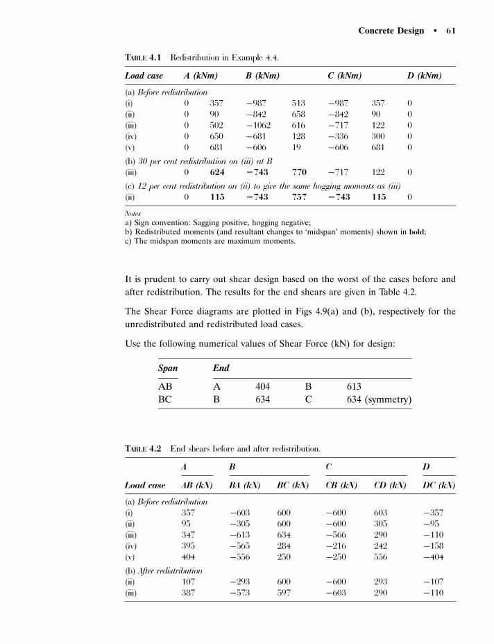
It is prudent to carry out shear design based on the worst of the cases before and
after redistribution. The results for the end shears are given in Table 4.2.
The Shear Force diagrams are plotted in Figs 4.9(a) and (b), respectively for the
unredistributed and redistributed load cases.
Use the following numerical values of Shear Force (kN) for design:
Span End
AB A 404 B 613
BC B 634 C 634 (symmetry)
TABLE 4.1 Redistribution in Example 4.4.
Load case A (kNm) B (kNm) C (kNm) D (kNm)
(a) Before redistribution(i) 0 357 �987 513 �987 357 0(ii) 0 90 �842 658 �842 90 0(iii) 0 502 �1062 616 �717 122 0(iv) 0 650 �681 128 �336 300 0(v) 0 681 �606 19 �606 681 0
(b) 30 per cent redistribution on (iii) at B(iii) 0 624 2743 770 �717 122 0
(c) 12 per cent redistribution on (ii) to give the same hogging moments as (iii)(ii) 0 115 2743 757 2743 115 0
Notesa) Sign convention: Sagging positive, hogging negative;b) Redistributed moments (and resultant changes to ‘midspan’ moments) shown in bold;c) The midspan moments are maximum moments.
TABLE 4.2 End shears before and after redistribution.
A B C D
Load case AB (kN) BA (kN) BC (kN) CB (kN) CD (kN) DC (kN)
(a) Before redistribution(i) 357 �603 600 �600 603 �357(ii) 95 �305 600 �600 305 �95(iii) 347 �613 634 �566 290 �110(iv) 395 �565 284 �216 242 �158(v) 404 �556 250 �250 556 �404
(b) After redistribution(ii) 107 �293 600 �600 293 �107(iii) 387 �573 597 �603 290 �110
Concrete Design � 61
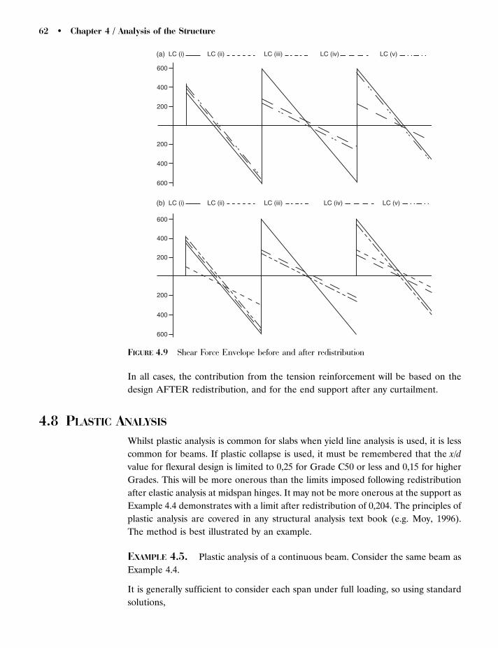
In all cases, the contribution from the tension reinforcement will be based on the
design AFTER redistribution, and for the end support after any curtailment.
4.8 PLASTIC ANALYSISWhilst plastic analysis is common for slabs when yield line analysis is used, it is less
common for beams. If plastic collapse is used, it must be remembered that the x/d
value for flexural design is limited to 0,25 for Grade C50 or less and 0,15 for higher
Grades. This will be more onerous than the limits imposed following redistribution
after elastic analysis at midspan hinges. It may not be more onerous at the support as
Example 4.4 demonstrates with a limit after redistribution of 0,204. The principles of
plastic analysis are covered in any structural analysis text book (e.g. Moy, 1996).
The method is best illustrated by an example.
EXAMPLE 4.5. Plastic analysis of a continuous beam. Consider the same beam as
Example 4.4.
It is generally sufficient to consider each span under full loading, so using standard
solutions,
LC (i) LC (ii) LC (iii) LC (iv) LC (v)
LC (i) LC (ii) LC (iii) LC (iv) LC (v)
600
400
200
200
400
600
(a)
(b)
600
400
200
200
400
600
FIGURE 4.9 Shear Force Envelope before and after redistribution
62 � Chapter 4 / Analysis of the Structure
Central 10 m span (Fig. 4.7(c)):
MSd ¼ qSdL2=16 ¼ 120 � 1022=16 ¼ 750 kNm
End 8 m span (Fig. 4.8(b)2):
MSd ¼ ð1,5 �ffiffiffi2
pÞqSdl
2 ¼ ð1,5 �p
2Þ � 120 � 82 ¼ 659 kNm
The individual spans do not collapse simultaneously. The centre span is critical as
the required design moment is higher. There are two alternative solutions that may
now be adopted.
(a) Accept that the centre of the 8 m span remains elastic with a design value
determined from Eq. (4.28)
Mmax ¼qL2
AB
8þMAB �MBA
2þ
1
2q
MAB þMBA
LAB
� �2
¼120 � 82
8þ�750
2þ
1
2 � 120
�750
8
� �2
¼ 622 kNm
at a position xmax from Eq. (4.29)
xmax ¼LAB
2þMAB þMBA
qLABþ
8
2�
750
120 � 8¼ 3:22 m
(b) The alternative is to keep the sagging moment in the end spans and the hogging
support moment as 659 kNm and to increase the midspan design moment in the
10 m span. The increased moment is given from Eq. (4.27) as
Mmid ¼qL2
AB
8þMAB �MBA
2
¼120 � 102
8þ�659 � 659
2¼ 841 kNm
For each solution, the resultant BMD’s and SFD’s are illustrated in Figs 4.7(d)
and (e), respectively.
From a practical point of view the second solution is probably preferable since the
hogging moment and hence the quantity of tension reinforcement in the top face is
reduced. The requirements for shear steel are unlikely to be much different as,
although the end reaction is slightly higher for (b), the tension steel requirement at
midspan is also higher. The second solution is slightly less satisfactory in fire as the
sagging moments will reduce faster than the hogging moments. If ‘deemed to satisfy’
clauses are used for the fire limit state, it would be prudent, although possibly
conservative, to use the data for simply supported beams.
Concrete Design � 63
REFERENCES AND FURTHER READING
Chana, P. and Clapson, J. (1992) Innovative shearhoop system for flat slab construction. Concrete,
26(1), 21–24.
EN 1990: Eurocode – Basis of structural design.
ISE (2002) Safety in Tall Buildings and Other Buildings with Large Occupancy. Institution of
Structural Engineers.
Mlakar, P.F., Dusenberry, D.O., Harris, J.R., Haynes, G., Phan, L.T. and Sozen, M.A. (2003)
Pentagon Building Performance Report, Civil Engineering, 73(2), 43–55.
Moy, S.S.J. (1996) Plastic Methods for Steel and Concrete Structures (2nd Edn), MacMillan,
Hampshire, UK.
Oliviera, D.R.C., Regan, P.E. and Melo, G.S.S.A. (2004) Punching resistance of RC slabs with
rectangular columns. Magazine of Concrete Research, 56(3), 123–138.
Regan, P.E. (1981) Behaviour of Reinforced Concrete Flat slabs. CIRIA Report 89.
Wearne, P. (1999) Collapse – Why Buildings Fall Down. Channel 4 Books, London, UK.
Wood, J.G.M. (2003) Pipers Row Car Park Collapse: Identifying risk. Concrete, 37(9), 29–31
Yandzio, E. and Gough, M. (1999) Protection of Buildings against Explosions. SCI Publication
244, SCI.
64 � Chapter 4 / Analysis of the Structure

C h a p t e r 5 / Durability, Serviceabilityand Fire
Traditionally engineers have been content to consider the control of durability using
‘deemed to satisfy’ approaches with respect to phenomena such as cracking or
deflection. This traditional approach, although still valid, needs to be supplemented
by more fundamental approaches. For a large number of cases, control of cracking
or deflection by bar spacing rules or span to effective depth ratios is satisfactory, but
where control of cracking is vital to the use or appearance of a structure, calculations
may become necessary. Further in order to allow the formulation of simple rules,
assumptions need to be made which are conservative in nature, thus it may be more
economic in the use of materials to use more rational methods to assess, say,
deflections.
Further, one of the major problems besetting concrete structures are those due to
loss of durability through reinforcement corrosion, alkali aggregate reaction or
sulfate attack at an age below the design life of the structure.
5.1 MECHANISMS CAUSING LOSS OF DURABILITY
The ideal situation would be to be able to determine when loss of durability would
occur such that acceptable limits were breached, i.e. durability would become a true
limit state phenomenon. In practice, the requirements for detailing such as cover are
set to ensure that the loss of durability should not occur within the service life of the
structure, provided there is good quality assurance on the concrete and on site
procedures to ensure that specified cover is met (Clark et al., 1997). The major
concerns with loss of durability are corrosion of the reinforcement, alkali-aggregate
reaction and sulfate attack. The Concrete Society have issued a Technical Report
(Bamforth, 2004) which provides an excellent background to measures which may
be taken to enhance durability.
5.1.1 Reinforcement Corrosion
At its extreme, corrosion of the reinforcement will lead to spalling of the concrete
cover with the resultant exposure of such reinforcement, together with loss in
strength of the structural member as all or part of the cross-sectional area of the
rebar is lost. In a less extreme form, unsightly surface rust staining will occur. When
the first signs of spalling are observed it will often be too late to combat corrosion
and recourse will be needed to expensive remedial repairs or mitigation. In the
ultimate case, expensive and often very difficult replacement of the structural
member will be necessary. Spalling occurs as the chemical products of the corrosion
reaction occupy a larger volume than the original rebar.
Corrosion occurs when the pH value of the concrete reduces from its original high
value of around 13 during placing to below 9 at a later stage (Page and Treadaway,
1982). This change in pH is known as a loss in passivity and is due to two possible
causes:
(a) Carbonation, and
(b) Chloride attack.
5.1.1.1 Carbonation
This is a gradually occurring attack caused by the penetration of acidic gasses
(mostly carbon dioxide) and reaction with any free alkali present. This reaction
lowers the pH value. Since the mechanism is diffusion controlled, the depth of
carbonation is proportional to the square root of time. The covers to reinforcement
specified in EN 1992-1-1 are such that for good quality concrete the depth of
carbonation during the design service life of the structure should not depassify the
concrete between the concrete surface and any rebar. The process of carbonation is
illustrated in Fig. 5.1.
The minimum cover cmin,dur required by EN 1992-1-1 together with the environmental
conditions and structure classification applicable to each are summarized in Table 5.1.
The standard structure classification is Class 4 (design life of 50 years). However, the
structure classification is adjusted for parameters such as increased design life,
higher strength concretes than those noted in Table 5.1, slab type elements, and
special quality control. Increasing the design life to 100 years increases the structure
classification to two levels higher and the remaining factors reduce the structure
classification by one level lower. The actual cover required cmin is given by
cmin ¼ max½cmin ,b; cmin ,dur þ�cdur,� ��cdur,st ��cdur,add: 10mm� ð5:1Þ
where cmin,b is the minimum cover due to bond requirement, �cdur,� additive safety
element (recommended value of zero), �cdur,st reduction in cover due to use of
stainless steel (recommended value of zero), and �cdur,add reduction due to use of
66 � Chapter 5 / Durability, Serviceability and Fire

additional protection (recommended value is zero). The minimum cover due to
bond cmin,b for reinforced concrete is bar diameter for separated bars and equivalent
diameter given by �n¼�/ffiffiffin
pb (� 55 mm) where n is the number of bars (from
Table 4.2 of EN 1992-1-1). For prestressed concrete, it is the duct diameter for
circular post tensioning ducts, twice the diameter of pretensioning strand or 3 times
the diameter of indented wire.
The nominal cover cnom used in design is given by
cnom ¼ cmin þ�cdev ð5:2Þ
The recommended value for �cdev is 10 mm, although the code does allow
reductions where there is a quality control system (more likely in precast concrete)
or where a very accurate device is used for monitoring and any resulting non-
conforming items rejected.
The covers specified in Table 5.1 are only adequate when the concrete has the
requisite low coefficient of permeability. This can only be ensured if the concrete has
a sufficiently high workability to enable the concrete to be properly placed and
vibrated. Workability should be controlled through the use of admixtures such as
plasticisers or super-plasticisers and NOT by the addition of extra water which may
give problems with shrinkage cracking (also causing potential loss in durability
Exposedsurface
Carbonationzone
Aggregate
Reinforcement
(b) Corrosion in carbonated concrete
Carbonationzone
Rustpatches
(a) Partially carbonated concrete
FIGURE 5.1 Corrosion due to carbonation
Concrete Design � 67

unless designed for). It is therefore essential when detailing the reinforcement,
especially at laps including those between starter bars and main bars to ensure the
concrete can flow. Construction joints which are often at points of high internal
forces are also areas where the concrete quality needs considering as honeycombing
will give a high coefficient of diffusion and thus allow easy ingress of carbon dioxide
or chloride-bearing fluids.
Problems with construction joints can also be eased by kickerless construction
methods and the use of retarding agents to delay the initial set of the concrete.
A further influence on achieving acceptable levels of permeability is adequate curing
of the concrete. Concrete which is not properly cured is a potential source for
concern. The economics of modern construction has forced reductions in times before
the formwork is struck. EN 206-1 provides some data on minimum curing times
related to ambient conditions, concrete temperature during curing and rate of strength
development. The earlier the formwork is struck, the more the surface-free water will
evaporate rather than combine chemically with the cement. It is this surface layer
which is important to ensure the concrete member is relatively impermeable.
The reduction of striking times has been made possible by grinding Ordinary Portland
Cements (OPC) very fine, thereby increasing the specific surface area and increasing
hydration rates, and turning OPC’s into effectively Rapid Hardening Cements (RHC).
This increase in hydration is also made possible by increasing the proportion of C3A
in the cement. Drawbacks to this trend are the resultant increase in heat of hydration
and early thermal or shrinkage cracks and that at normal ages the concrete strength
becomes potentially high enough to cause spalling problems in fire (Bailey, 2002).
Beeby (1978) has indicated that cracking parallel to the rebar is more harmful in
corrosive conditions than that of the normal to the bar, as such cracking allows an
TABLE 5.1 Minimum Covers cdur,min (mm) for reinforced concrete.
Structure class
ExposureClass
Environment and typeS1 S2 S3 S4 S5 S6
Min strengthclass
X0 Unreinforced; reinforced in buildings 10 10 10 10 15 20 C30/37XC1 Dry; permanently wet low humidity 10 10 10 15 20 25 C30/37XC2/XC3 Wet, rarely dry; foundations;
external sheltered concrete10 15 20 25 30 35 C35/45
XC4 Cyclic wetting and drying 15 20 25 30 35 40 C40/50XD1 Airborne chlorides 20 25 30 35 40 45 C40/50XS1 Airborne salt � near to coast 20 25 30 35 40 45 C40/50XD2 Swimming pools; industrial chlorides 25 30 35 40 45 50 C40/50XS2 Permanently submerged in sea 25 30 35 40 45 50 C45/55XD3 Cyclic due to chloride spray 30 35 40 45 50 55 C45/55XS3 Marine tidal and splash zones 30 35 40 45 50 55 C45/55
68 � Chapter 5 / Durability, Serviceability and Fire

easier path to the surface of the bar. Such parallel cracks are generally due to
shrinkage or early thermal movement and can be reduced by the provision of
adequate distribution reinforcement. Such reinforcement is more effective when it is
of small diameter at relatively low spacing, and may need to exceed the minimum
laid down in any design code.
5.1.1.2 Chloride Attack
Some free chloride ions exist in the hydrating cement but in low proportions. The
once historically popular use of admixtures containing CaCl2 is now expressly
forbidden, but contaminants containing chlorides can still be introduced when sea-
dredged aggregates or sea water is used in the production of concrete. Both these
should be avoided wherever possible. However, two possible sources of chloride
ingress cannot be avoided. These are where the structure is exposed to a marine
environment or to de-icing salts on highways. The major problem with both these is
chloride ingress through cracks parallel to rebar (Fig. 5.2), and it is thus necessary to
control the width of such cracks by explicit calculations.
5.1.2 Alkali-Aggregate Reaction
In this case a chemical reaction occurs between the alkalinity of the pore water
(usually Na2O or K2O), due either to alkaline elements within the cement or an
external source such as sea water or de-icing salts, and certain types of silica in the
aggregate (this is known as Alkali–Silica Reaction, or ASR). The reaction causes a
positive volume change with associated microcracking, which will eventually result in
loss of cover to the rebar. Most, but not all, British aggregates are not susceptible to
this type of reaction. Unfortunately, there is no simple test to determine any such
susceptibility, and thus care needs taking to limit the alkali content of the mix, the
effective alkali content of the cement itself and where the structural element is
exposed to an alkaline environment, consideration should be given to provision of
an impermeable surface membrane. The alkali content of a cement can be reduced
by using a cement replacement such as Pulverized Fuel Ash (PFA) or Ground
Granulated Blast Furnace Slag (GGBFS), both of which are industrial waste
Exposed surface Crack
Carbonation zone
Reinforcing bar
Rust scale FIGURE 5.2 Corrosionin cracked concrete
Concrete Design � 69

products. Both these replacements slow down the rate of strength gain in the
concrete and additionally have a lower heat of hydration, thus reducing early
thermal shrinkage and cracking. Recent guidance on ASR has been published by
BRE in Digest 330 (BRE, 2004).
5.1.3 Sulfate Attack
This occurs due to attack from free sulfates contained in groundwater or soil, and is
therefore generally limited either to buried structures including foundations or
structures in an aggressive environment where sulfates are naturally present, e.g.
certain types of sewage, industrial effluent or chemical process plants. It is generally
sufficient to combat sulfate attack by using Sulfate-Resisting Portland Cements
(SRPC). In these cases, the requirement to ensure the existence of low permeability
concrete in the structure is paramount as any ingress of sulfates should be prevented
(Dunster and Crammond, 2003).
5.1.4 Taumasite Attack
This phenomenon is caused by a chemical reaction between cement and certain
types of clay in the presence of groundwater. It will therefore affect foundations or
buried concrete. Fortunately the types of clay involved only occur in limited areas
and thus the phenomenon is not widespread (Taumasite Experts Group, 1999). A
useful overview of concrete deterioration, methods of overcoming it and specialist
techniques for concrete below ground is given in a CIRIA Report (Henderson et al.,
2002).
5.2 SERVICEABILITY LIMIT STATESAs mentioned in Chapter 1, these are simply a series of criteria which are applied to
the performance of the structure during its normal working life under the action of
service (or working) loads or actions.
For the majority of structures, the two most important criteria are deflections and
crack widths. These both help ensure that durability is not unduly impaired and that
the structure has no visible damage (or detrimental effects). In some cases, vibration
response needs to be considered where machinery is involved or where wind loading
can cause vortex shedding and subsequent oscillatory motion (Tacoma Narrows
Suspension Bridge). Concrete structures other than some footbridges are seldom
slender enough to cause problems under normal variable loading. A recent, but,
classic case of such problems occurring was the Millennium Bridge in London
described in Dallard et al. (2001). In all cases, it is necessary for the engineer to
70 � Chapter 5 / Durability, Serviceability and Fire
assess the risks of any phenomenon likely to affect any structure and then carry out
any requisite design checks.
The design for fire resistance has been included in this chapter partly because the
subject can be handled using simple clauses specifying member thicknesses or rebar
cover (as in durability) and partly because, although fire is an ultimate accidental
limit state in that collapse is being considered, loading lower than that at ULS is used
to determine the internal stress resultants.
5.2.1 Deflections
In general structural deflections are traditionally limited to span/250, although
where partitions or finishes may be damaged, this limit is reduced to span/500
(cl 7.4.1). The deflections may be controlled either by the use of span/effective
depth ratios or by explicit calculations.
5.2.1.1 Span/Effective Depth Ratios
This approach can be justified in outline as follows:
For any beam the midspan deflection � for a given loading pattern is obtained from
� ¼ k1W L3
EsIsð5:3Þ
where k1 is a coefficient dependant upon the loading pattern and the support
conditions, W the total service load, L the span, and EsIs is flexural rigidity of the
section in ‘steel’ units (assumed constant at the value obtaining at the maximum
moment).
The maximum moment Ms is given by
Ms ¼ k2 W L ð5:4Þ
where k2 is a factor dependant upon the load pattern.
The stress in the tensile reinforcement s is given by
s ¼Msðd� xÞ
Isð5:5Þ
where d is the effective depth and x the depth to the neutral axis.
Substitute Eqs (5.4) and (5.5) into Eq. (5.3) to give
�
L¼
k1
k2
s
d� x
L
dð5:6Þ
Concrete Design � 71

Equation (5.6) indicates that if the deflection requirement is expressed as a fraction
of the span, then it is directly related to the span/effective depth ratio and is also a
function of the stress level in the reinforcement.
The method used in EN 1992-1-1 is to take basic span/effective depth ratios and
modify them appropriately to allow for factors such as type of reinforcement
(cl 4.4.3.2).
The basic K factors for deflection are given in Table 5.2 (from Table 7.4N of EN
1992-1-1).
The Code indicates that the span effective depth ratios have been obtained from a
parametric study and correspond to a service stress in the reinforcement of 310 MPa
(with a yield stress of 500 MPa).
The basic span effective depth ratio l/d is given by,
for � 0
l=d ¼ K 11 þ 1,5ffiffiffiffiffifck
p 0
� �þ 3,2
ffiffiffiffiffifck
p 0
� 1
� �1,5" #
ð5:7Þ
and for 4 0
l=d ¼ K 11 þ 1,5ffiffiffiffiffifck
p 0
� 0
� �þ
1
12
ffiffiffiffiffifck
p ffiffiffiffiffi0
0
r� �ð5:8Þ
where 0 is a reference steel ratio defined as 0,001ffiffiffiffiffifck
p, fck the characteristic
strength of the concrete, the tensile steel ratio (¼As/bd) and 0 the compressive
steel ratio (¼As0/bd). The values of and 0 are based the required values of
As and As0, respectively.
TABLE 5.2 Recommended Basic K values for deflection (from Table 7.4N of EN 1992-1-1).
K
l/d
q¼ 1,5 % q¼ 0,5 %
Simply supported beamOne or two way simply supported slab 1,0 14 20
End span of a continuous beam orone way spanning slabTwo way spanning slab continuous
over the long edge
1,3 18 26
Interior span of continuous beam or slab 1,5 20 30Flat slab (longer span) 1,2 17 24Cantilever 0,4 6 8
Note: the reinforcement ¼ 0,5% represents lightly stressed concrete members and ¼ 1,5%represents highly stressed concrete members.
72 � Chapter 5 / Durability, Serviceability and Fire

For two way spanning slabs, the shorter span is used to determine the critical span/
effective depth ratio, but for flat slabs the larger span should be taken.
Additional modifications may be made for
� Geometry
The values from Eqs (5.7) or (5.8) are multiplied by a factor when
flanged sections are used. The factor takes a value of 0,8 for beff/bw� 3, and 1
for beff/bw¼ 1,0, where beff is the effective width of the flange (Section 6.4) and
bw the web width. Linear interpolation can be used between these values such that
the factor is given by
0,8 þ 0,1 3 �beff
bw
� �� 0,8 ð5:9Þ
� Reinforcement stress levels
As noted above, the tabular values have been based on a service stress s in the
reinforcement of 310 MPa, corresponding to the service stress taken as
approximately (5/8)fyk with a reinforcement strength of 500 MPa.
For reinforcement with other characteristic strengths, the tabular values should be
multiplied by a factor 310/1 given by
310
s¼
500
fykðAs,req=As,provÞ¼
500
fyk
As,prov
As,reqð5:10Þ
where fyk is the characteristic strength in the reinforcement, As,req is the area of
tension reinforcement required to resist the applied moment and As,prov is the
actual amount of tensile steel. This latter correction factor takes account of the fact
that any extra reinforcement over that actually needed will reduce the service stress
in the steel by increasing the second moment of area.
Additionally, where supporting partitions (or finishes) may be damaged by excessive
deflections the values from Eqs (5.7) or (5.8) should be multiplied by 7/leff for beams
and slabs (other than flat slabs) with spans exceeding 7 m, and for flat slabs where
the greater span leff exceeds 8,5 m, by 8,5/leff, where leff is the effective span.
EXAMPLE 5.1 Deflection control using span/effective depth ratios. Check the
design of the cantilever shown in Fig. 5.3 is suitable.
As,prov=bd ¼ 5026=635 � 370 ¼ 0,0214
¼ As,req=bd ¼ 3738=635 � 370 ¼ 0,0159
A0s=bd ¼ 1608=635 � 370 ¼ 0,00684
fck ¼ 25 MPa, 0 ¼ 0,001ffiffiffiffiffifck
p¼ 0,001 �
ffiffiffiffiffi25
p¼ 0,005
Concrete Design � 73
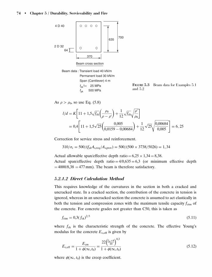
As 4 0, so use Eq. (5.8)
l=d ¼ K 11 þ 1,5ffiffiffiffiffifck
p 0
� 0
� �þ
1
12
ffiffiffiffiffifck
p ffiffiffiffiffi0
0
r� �
¼ 0,4 11 þ 1,5ffiffiffiffiffi25
p 0,005
0,0159 � 0,00684
� �þ
1
12
ffiffiffiffiffi25
pffiffiffiffiffiffiffiffiffiffiffiffiffiffiffiffi0,00684
0,005
s" #¼ 6; 25
Correction for service stress and reinforcement.
310=s ¼ 500=ðfykAs,req=As,provÞ ¼ 500=ð500 � 3738=5026Þ ¼ 1, 34
Actual allowable span/effective depth ratio¼ 6,25� 1,34¼ 8,38.
Actual span/effective depth ratio¼ 4/0,635¼ 6,3 (or minimum effective depth
¼ 4000/8,38 ¼ 477 mm). The beam is therefore satisfactory.
5.2.1.2 Direct Calculation Method
This requires knowledge of the curvatures in the section in both a cracked and
uncracked state. In a cracked section, the contribution of the concrete in tension is
ignored, whereas in an uncracked section the concrete is assumed to act elastically in
both the tension and compression zones with the maximum tensile capacity fctm of
the concrete. For concrete grades not greater than C50, this is taken as
fctm ¼ 0,3 fckð Þ2=3
ð5:11Þ
where fck is the characteristic strength of the concrete. The effective Young’s
modulus for the concrete Ec,eff is given by
Ec,eff ¼Ecm
1 þ �ð1, t0Þ¼
22 fckþ810
� �0,3
1 þ �ð1, t0Þð5:12Þ
where �(1, t0) is the creep coefficient.
4 D 40
2 D 3264
370
Beam cross section
Beam data : Transient load 40 kN/m
Permanent load 30 kN/m
Span (Cantilever) 4 m
25 MPa500 MPa
fck1<fyk
635700
FIGURE 5.3 Beam data for Examples 5.1and 5.2
74 � Chapter 5 / Durability, Serviceability and Fire

The curvature (or other appropriate deformation parameter) � under any condition
is given by
� ¼ ��II þ ð1 � �Þ�I ð5:13Þ
where �I is calculated on the uncracked section, �II is calculated on the cracked
section, and � is a distribution parameter which allows for tension stiffening and is
given by
� ¼ 1 � �sr
s
� �2
ð5:14Þ
where � allows for the duration of the loading and is 1,0 for a single short term load
and 0,5 for sustained or repetitive loading, s is the stress in the steel calculated on a
cracked section and sr is the stress in the steel as the section is just about to crack.
Beeby, Scott and Jones (2005) suggest that as the decay of tensile stress is relatively
fast (i.e. a matter of hours), then � should always be taken as 0,5. In flexure, the ratio
s/sr can be replaced by M/Mcr (where Mcr is the moment which just causes
cracking) or in tension by N/Ncr (where Ncr is the force which just causes cracking).
For an uncracked section � is zero.
The curvature due to shrinkage (1/rcs) is given by
1
rcs¼ "cs�e
S
Ið5:15Þ
where "cs is the shrinkage strain, �1 the modular ratio (defined as Es/Ec,eff), S the
first moment of area of the reinforcement about the centroidal axis and I the
second moment of area. Both S and I should be calculated for the cracked and
uncracked section and combined using Eq. (5.13) with � replaced by 1/rcs.
The section properties required are determined as follows:
(a) Uncracked section (Fig. 5.4):
In an uncracked section the concrete is taken as linear elastic with equal Young’s
moduli for both compression and tension. The reinforcement will be linear
elastic.
d
x
b
Ast r = Ast / bd
ae = Es / Ec
r¢ = Asc / bd Asc
d ¢
FIGURE 5.4 Cross section data
Concrete Design � 75

The second moment of area Igross is given by
Igross
bd3¼
1
3
x
d
� �3þ
1
3
h
d�
x
d
� �3
ð5:16Þ
where x/d is given by
x
d¼
1=2 h=dð Þ2þ �e
0ðd0=dÞ þ ð Þ
ðh=dÞ þ �e 0 þ ð Þð5:17Þ
The uncracked moment Muncr that can be taken by the section is given by
Muncr ¼fctIgross
h� xð5:18Þ
where fct is the relevant tensile stress in the concrete, and the curvature 1/rM,uncr
is given by
1
rM,uncr¼
1
h� x
fct
Ec,effð5:19Þ
The moment Mcr and curvature 1/rcr at the point of cracking is obtained by
setting fct¼ fctm in Eq. (5.19).
(b) Cracked section:
In a cracked section, the concrete is taken as linear elastic in compression and
cracked in tension. The reinforcement will be linear elastic.
The second moment of area Icr is given by
Icr
bd3¼
1
3
x
d
� �3þ0�e
x
d�d0
d
� �2
þ�e 1 �x
d
� �2ð5:20Þ
where x/d is given by,
x
d¼ ��e
0 þ ð Þ þ �2e
0 þ ð Þ2þ2�e 0
d0
dþ
� �� �0,5
ð5:21Þ
The moment Mcr taken by the section is given by
Mcr ¼fcsIcr
xð5:22Þ
where fcs is the compressive stress in the concrete, and the curvature 1/rcr is
given by
1
rM,cr¼
1
x
fcs
Ec,effð5:23Þ
76 � Chapter 5 / Durability, Serviceability and Fire

Where there is no compression steel Eqs (5.20) and (5.21), reduce to
Icr
bd3¼
1
3
x
d
� �3þ�e 1 �
x
d
� �2ð5:24Þ
where x/d is given by,
x
d¼ ��eþ �2
e2 þ 2�e
� 0,5¼ �e
ffiffiffiffiffiffiffiffiffiffiffiffiffiffiffiffi1 þ
2
�e
s� 1
" #ð5:25Þ
The resultant deflections can be determined using two methods of deceasing
accuracy:
� Integration of the curvatures calculated at discrete increments along the length of
the member,
� direct use of the curvature at the point of maximum moment interpolating
between the cracked and uncracked values section using Eq. (5.13).
In the exact method, the total curvature 1/rtot at any point is related to the deflection
w by the following expression
1
rtot¼
d2w
dx2ð5:26Þ
The second order differential can be replaced by its finite difference form to give
1
rtot¼
wxþ1 þ wx�1 � 2wx
�xð Þ2
ð5:27Þ
where the deflections are determined at the point x and either side of it, and � x is
the incremental length along the beam between points at which the curvature is
calculated. For a simply supported (or continuous) beam the deflections are zero at
the supports and for a cantilever the deflection and slope are zero at the (encastre)
support.
In the approximate method, the deflections are calculated assuming the whole
member is either cracked or uncracked and the resultant deflection determined
using the maximum curvature derived from substituting Eq. (5.4) into Eq. (5.3),
� ¼k1
k2
M
EIL2 ¼ k3
1
rL2 ð5:28Þ
where k3 depends on the loading pattern and L is the span. For common load cases,
values of k3 are given in Fig. 5.5.
Concrete Design � 77

EXAMPLE 5.2 Deflection calculations. Determine the actual deflection for the
cantilever shown in Fig. 5.3.
Basic data:
fctm ¼ 0,30f 2=3ck ¼ 0,30 � 252=3 ¼ 2,56 MPa:
Ecm ¼ 22ðð fckþ8Þ=10Þ0,3¼ 22ðð25 þ 8Þ=10Þ0,3
¼ 31,5 GPa:
Loading
W
W / 2 W / 2
αL
αL αL
αL αL
αL
αL
q
q
A BC
W
W
q
q
M
W
(α − 1) L
(1−2α) L
(1−2α) L
( − )
( − )
( + )
( + )
( + )
M
M
Wα( 1 − α ) L( 3-4α2 ) /48 ( 1 − α )
0.125 − α2/6
0.0625
5 / 48
0.102
( 5 − 4α2 )2/80 ( 3 − 4α2 )
α (3 − α ) / 6
α (4 − α ) / 12
k = 0.083 (1−b / 4 )b = ( MA + MB ) / MCnumerical values of MA etc.are usedk = 0.104 (1−b / 10 )b = ( MA + MB ) / MCMC may be either the midspanor maximum value, any errorwill be small
0.125
k3BMD
MC
MC
MB
MB
MA
MA
W α L
WL2
24( 3−4α2 )
q L2 / 15.6
q L2 / 8
Wα L / 2
q α2 L2 / 2
FIGURE 5.5 Values of coefficient k3 for deflection calculations
78 � Chapter 5 / Durability, Serviceability and Fire
Shrinkage strain (Table 3.2 EN 1992-1-1):
The shrinkage strain "cs comprises two components: drying shrinkage ("cd) and
autogenous shrinkage ("ca).
Drying shrinkage "cd:
Assuming 40 per cent relative humidity, the nominal shrinkage strain "cd,0 is
0,60�10�3. Assume loading is at 28 days (i.e. t¼ 28) and that curing finished at a
time of 3 days (i.e. ts¼ 3), then the shrinkage strain at time of loading is
"cdðtÞ ¼ �dsðtÞkh"cd,0
where kh is a parameter dependant upon the notional size h0 given by 2Ac /u, and
�ds(t,ts) is given by
�dsðt, tsÞ ¼t� ts
t� ts þ 0,04
ffiffiffiffiffiffiffiffiffiffiffiffiffiffiffiffi2Ac
u
� �3s
where Ac is the concrete gross sectional area and u is the perimeter exposed to
drying.
h0 ¼ 2 � ð700 � 370Þ=ð2ð700 þ 370ÞÞ ¼ 242 mm:
From Table 3.3 (EN 1992-1-1), kh¼ 0,808 (by linear interpolation)
�dsðt, tsÞ ¼28 � 3
28 � 3 þ 0,04ffiffiffiffiffiffiffiffiffiffi2423
p ¼ 0,142
So, "cd(t)¼ 0,142� 0,808� 0,60� 10�3¼ 69� 10�6
Autogenous shrinkage strain, "ca:
"caðtÞ ¼ �asðtÞ"cað1Þ
where the limiting autogenous shrinkage strain "ca(1) is given by
"cað1Þ ¼ 2,5ð fck � 10Þ � 10�6
¼ 2,5ð25 � 10Þ � 10�6 ¼ 37,5 � 10�6
the loading correction factor �as(t) is given by
�asðtÞ ¼ 1 � e�0,2t0,5
¼ 1 � e�0,2�280,5
¼ 0,653
Thus, the autogenous shrinkage strain "ca,
"caðtÞ ¼ �asðtÞ"cað1Þ
¼ 0,653 � 37,9 � 10�6 ¼ 24 � 10�6
Concrete Design � 79

The total shrinkage strain "cs:
"cs ¼ "cd þ "ca ¼ 69 � 10�6 þ 24 � 10�6
¼ 93 � 10�6
Creep coefficient �(t,t0):
Use Annex B of EN 1992-1-1:
�ðt,t0Þ ¼ �0�cðt,t0Þ
where the basic creep coefficient �0 is given by
�0 ¼ �RH�ð fcmÞ�ðt0Þ
For concrete grade C25, �RH is given by
�RH ¼ 1 þ1 � RH=100
0,1ffiffiffiffiffih0
3p
¼ 1 þ1 � 40=100
0,1ffiffiffiffiffiffiffiffi2423
p ¼ 1,963
The modification factor for mean concrete strength, �( fcm):
�ð fcmÞ ¼16,8ffiffiffiffiffiffifcm
p ¼16,8ffiffiffiffiffiffiffiffiffiffiffiffiffiffi25 þ 8
p ¼ 2,92
The correction factor for the time of loading of the element �(t0):
�ðt0Þ ¼1
0,1 þ t0,200
¼1
0,1 þ 30,20¼ 0,445
or �0 is given as
�0 ¼ �RH�ð fcmÞ�ðt0Þ
¼ 1,963 � 2,92 � 0,445 ¼ 2,55
The factor �(t,t0) to allow for the time relation between time at loading t0 and time
considered, t, is given by
�cðt,t0Þ ¼t� t0
�H þ t� t0
� �0,3
80 � Chapter 5 / Durability, Serviceability and Fire

where for concrete grade less than C35, �H is given by
�H ¼ 1,51 þ ð0,012RHÞ
18
h0þ 250
¼ 1,51 þ ð0,012 � 40Þ18
242þ 250 ¼ 613
Thus �(t,t0) is
�cðt,t0Þ ¼t� t0
�H þ t� t0
� �0,3
¼28 � 3
613 þ 28 � 3
� �0,3
¼ 0,378
so �(t,t0) becomes
�ðt,t0Þ ¼ �0�cðt,t0Þ ¼ 2,55 � 0,378 ¼ 0,964
Ec,eff ¼ Ecm=ð1 þ �ðt,t0ÞÞ ¼ 31,5=ð1 þ 0,964Þ ¼ 16,04 GPa:
�e ¼ 200=16,04 ¼ 12,5
Determine the cracked and uncracked second moments of area:
0 ¼ A0s=bd ¼ 1608=635 � 370 ¼ 0,0068;
¼ As=bd ¼ 5026=635 � 370 ¼ 0,0214;
d0=d ¼ 64=635 ¼ 0,101; h=d ¼ 700=635 ¼ 1,102
� ¼ 0, 5 ðsustained loadsÞ
Uncracked section:
Use Eq. (5.17) to determine x/d:
x=d ¼ ð0,5 � 1,1022þ12,5ð0,0214 þ 0,0068 � 0,101ÞÞ= . . .
ð1,102 þ 12,5ð0,0068 þ 0,0214ÞÞ ¼ 0,607
x ¼ 0; 607 � 635 ¼ 385 mm
and Eq. (5.16) for Igross,
Igross=bd3 ¼ 0,6073=3 þ ð1,102 � 0,607Þ3=3 þ 12,5 � 0,0068
ð0,607 � 0,101Þ2 þ 12,5 � 0,0214ð1 � 0,607Þ2 ¼ 0,178
Igross ¼ 0,178 � 370 � 6353 ¼ 16,86 � 109 mm4
Use Eq. (5.18) with fct replaced by fctm to determine Mcr
Mcr ¼ fctmIgross=ðh� xÞ ¼ 2,56 � 16,86 � 109=ð700 � 385ÞNmm ¼ 137 kNm:
Concrete Design � 81

Cracked section:
Use Eq. (5.21) to determine x/d
x=d ¼ �12,5ð0,0068 þ 0,0214Þ þ . . .ffiffiffiffiffiffiffiffiffiffiffiffiffiffiffiffiffiffiffiffiffiffiffiffiffiffiffiffiffiffiffiffiffiffiffiffiffiffiffiffiffiffiffiffiffiffiffiffiffiffiffiffiffiffiffiffiffiffiffiffiffiffiffiffiffiffiffiffiffiffiffiffiffiffiffiffiffiffiffiffiffiffiffiffiffiffiffiffiffiffiffiffiffiffiffiffiffiffiffiffiffiffiffiffiffiffiffiffiffiffiffiffiffiffiffiffiffiffiffiffiffiffiffiffið12,52ð0,0068 þ 0,0214Þ2þ2 � 12,5ð0,0068 � 0,101 þ 0,0214ÞÞ
q¼ 0,470
x ¼ 0,470 � 635 ¼ 298 mm
and Eq. (5.20) to determine Icr
Icr=bd3 ¼ 0,473=3 þ 12,5 � 0,0068ð0,101 � 0,47Þ2 þ 12,5 � 0,0214ð1 � 0,47Þ2¼ 0,121
Icr ¼ 0,121 � 370 � 6353¼ 11,46 � 109 mm4
Shrinkage parameters:
"cs�e¼ 93 � 10�6� 12,5 ¼ 1163 � 10�6
Calculate S/bd2:
Uncracked section:
S=bd2 ¼ 0,0214ð1 � 0,607Þ � 0,0068ð0,101 � 0,607Þ ¼ 0,0119
S ¼ 0,0119 � 370 � 6352¼ 1,775 � 106 mm3
S=Igross ¼ 1,775 � 106=16,86 � 109¼ 0,1053 � 10�3=mm
Cracked section:
S=bd2 ¼ 0,0214ð1 � 0,47Þ � 0,0068ð0,101 � 0,47Þ ¼ 0,0139
S ¼ 0,0139 � 370 � 6352¼ 2,074 � 106 mm3
S=Icr ¼ 2,074 � 106=11,46 � 109¼ 0,181 � 10�3=mm
Integration method:
Divide the beam into four segments each 1 m long (x¼ 0 at free end)
Total UDL (assuming the whole of the transient load acts on a quasi-permanent
basis) ¼ 40þ 30¼ 70 kN/m
MSd¼ 70x2/2¼ 35x2 kNm.
As the curvature 1/rcs on the cracked and uncracked sections is constant along the
beam these may be determined first.
Shrinkage:
Uncracked section:
1=rcs,unc ¼ ð"cs�eÞðS=IÞunc¼ 0,001163 � 0,1053 � 10�3
¼ 0,1225 � 10�6=mm
82 � Chapter 5 / Durability, Serviceability and Fire

Cracked:
1=rcs,cr¼ ð"cs�eÞðS=IÞcr¼ 0,001163 � 0,181 � 10�3
¼ 0,211 � 10�6=mm
Point 1 (x¼ 0): curvature is zero (zero moment)
Point 2 (x¼ 1)
MSd¼ 35 kNm5Mcr, thus �¼ 0:
Bending curvature:
fct¼MSdðh� xÞ=Igross¼ 35 � 106� ð700 � 385Þ=16,89 � 109
¼ 0,653 MPa
1=rM,unc ¼ ð fct=Ec,effÞ=ðh� xÞ ¼ ð0,653=16,04 � 103Þ=ð700 � 385Þ
¼ 0,129 � 10�6=mm
Total uncracked curvature, 1/rI:
1=rI ¼ 1=rcs,unc þ 1=rM,unc ¼ ð0,129 þ 0,1225Þ � 10�6¼ 0,252 � 10�6=mm
As the concrete is uncracked, 1/rtot¼ 1/rIPoint 3 (x¼ 2)
MSd ¼ 140 kNm4Mcr, thus � needs calculating:
s=sr ¼ MSd=Mcr ¼ 140=137 ¼ 1,022
Use Eq. (5.14) to calculate �:
� ¼ 1 � 0,5=1,0222¼ 0,478
Uncracked curvatures:
Bending:
fct ¼MSdðh� xÞ=Igross ¼ 140 � 106� ð700 � 385Þ=16,89 � 109
¼ 2,61 MPa
1=rM,unc ¼ ðfct=Ec,effÞ=ðh� xÞ ¼ ð2,61=16,04 � 103Þ=ð700 � 385Þ
¼ 0,517 � 10�6=mm
Total uncracked curvature 1/rI:
1=rI¼ 1=rcs,unc þ 1=rM,unc ¼ ð0,517 þ 0,1225Þ � 10�6¼ 0,640 � 10�6=mm
Cracked curvatures:
Bending:
fcs ¼ MSd x=Icr ¼ 140 � 106� 298=11,46 � 109
¼ 3,64 MPa
1=rM,cr ¼ ð fcs=Ec,effÞ=x ¼ ð3,64=16,04 � 103Þ=298 ¼ 0,762 � 10�6=mm
Concrete Design � 83

Total cracked curvature, 1/rII
1=rII ¼ 1=rcs,cr þ 1=rM,cr ¼ 0,762 � 10�6þ 0,211 � 10�6
¼ 0,973 � 10�6=mm
Effective total curvature 1/rtot is given by Eq. (5.13),
1=rtot¼ 0,478 � 0,973 � 10�6þð1 � 0,478Þ � 0,64 � 10�6
¼ 0,799 � 10�6=mm
Point 4 (x¼ 3)
MSd ¼ 315 kNm4Mcr, thus � needs calculating:
s=sr ¼ MSd=Mcr ¼ 315=137 ¼ 2,3
Use Eq. (5.14) to calculate �:
� ¼ 1 � 0,5=2,32¼ 0,906
Uncracked section:
Bending curvature:
fct ¼ MSdðh� xÞ=Igross ¼ 315 � 106� ð700 � 385Þ=16,89 � 109
¼ 5,87 MPa:
1=rM,unc ¼ ðfct=Ec,effÞ=ðh� xÞ ¼ ð5,87=16,04 � 103Þ=ð700 � 385Þ
¼ 1,162 � 10�6=mm
Total uncracked curvature 1/rI:
1=rI ¼ 1=rcs,uncþ1=rM,unc ¼ 1,162 � 10�6þ 0,1225 � 10�6
¼ 1,285 � 10�6=mm
Cracked section:
Bending:
fcs ¼ MSd x=Icr ¼ 315 � 106� 298=11,46 � 109
¼ 8,411 MPa
1=rM,cr ¼ ð fcs=Ec,effÞ=x ¼ ð8,411=16,04 � 103Þ=298 ¼ 1,760 � 10�6=mm
Total cracked curvature, 1/rII
1=rII ¼ 1=rcs,cr þ 1=rM,cr ¼ 1,760 � 10�6þ 0,211 � 10�6
¼ 1,971 � 10�6=mm
Effective curvature 1/rtot is given by Eq. (5.13),
1=rtot ¼ 0,906 � 1,971 � 10�6þ ð1 � 0,906Þ � 1,285 � 10�6
¼ 1,907 � 10�6=mm
84 � Chapter 5 / Durability, Serviceability and Fire

Point 5 (x¼ 4)
MSd ¼ 560 kNm4Mcr, thus � needs calculating:
s=sr ¼ MSd=Mcr ¼ 560=137 ¼ 4,088
Use Eq. (5.14) to calculate �:
� ¼ 1 � 0,5=4,0882 ¼ 0,970
Uncracked section:
Bending curvature:
fct ¼ MSdðh� xÞ=Igross ¼ 560 � 106� ð700 � 385Þ=16,89 � 109
¼ 10,44 MPa
1=rM,cr ¼ ð fct=Ec,effÞ=ðh� xÞ ¼ ð10,44=16,04 � 103Þ=ð700 � 385Þ
¼ 2,066 � 10�6=mm
Total uncracked curvature, 1/rI:
1=rI ¼ 1=rcs,unc þ 1=rM,unc ¼ 2,066 � 10�6þ 0,1225 � 10�6
¼ 2,189 � 10�6=mm
Cracked section:
fcs ¼ MSd x=Icr ¼ 560 � 106� 298=11,46 � 109
¼ 14,56 MPa
1=rII ¼ ð fcs=Ec,effÞ=x ¼ ð14,56=16,04 � 103Þ=298 ¼ 3,046 � 106=mm
Total cracked curvature 1/rII
1=rII ¼ 1=rcs,cr þ 1=rM,cr ¼ 3,046 � 106þ 0,211 � 10�6
¼ 3,257 � 106=mm
Effective curvature 1/rtot is given by Eq. (5.13),
1=rtot ¼ 0,970 � 3,257 � 106þ ð1 � 0,970Þ2,189 � 10�6
¼ 3,225 � 10�6=mm
The results from determining (� x)21/rtot at each node point are given in Table 5.3.
To allow the boundary conditions to be evaluated at point 5 in the beam, a fictitious
point 6 needs to be introduced (Fig. 5.6). The boundary conditions at node 5 are:
(a) deflection is zero, or w5¼ 0
(b) slope is zero, or (w6�w4)/(2� x)¼ 0; or, w6¼w4.
Thus applying Eq. (5.27) at each node point, together the boundary conditions,
gives in matrix form
AW ¼ � x2 1
rð5:29Þ
Concrete Design � 85

or, solving
W ¼ A�1� x2 1
rð5:30Þ
Substituting in numerical values gives,
21 �2
1 �2 11 �2 1
0BB@
1CCA
w1
w2
w3
w4
0BB@
1CCA ¼
3,2251,9070,7990,225
0BB@
1CCA
or
w ¼ 14,00 9,451 5,132 1,612ð Þ�1
Thus the deflection at the free end, w1¼ 14,0 mm.
This is equivalent to span/285 which is acceptable.
Approximate method:
The deflection w is given by Eq. (5.28). The calculation must be determined for
loading and shrinkage separately as each has different k3 factors.
For a UDL on a cantilever k3¼ 0,25 (Fig. 5.5).
TABLE 5.3 Deflection parameters for Example 5.2.
Node Point(�x)21/rtot(mm)
1 02 0,2523 0,7994 1,9075 3,225
where (�x)2¼ 10002
¼ 106 mm2.
w5 = Otgt
(6)
(∆x)
5 4
1000 1000 1000 1000 1000
32
1
[ w6 = w4 ]
w4
w3 w2 w1
FIGURE 5.6 Deflection profile for Example 5.2
86 � Chapter 5 / Durability, Serviceability and Fire
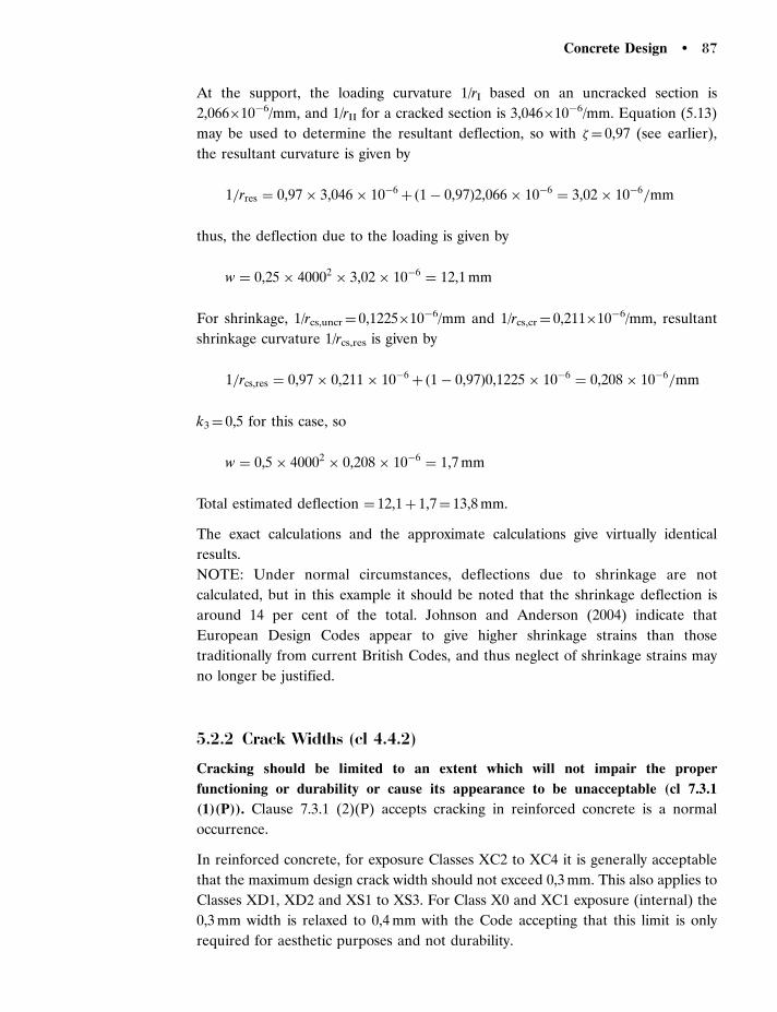
At the support, the loading curvature 1/rI based on an uncracked section is
2,066�10�6/mm, and 1/rII for a cracked section is 3,046�10�6/mm. Equation (5.13)
may be used to determine the resultant deflection, so with �¼ 0,97 (see earlier),
the resultant curvature is given by
1=rres ¼ 0,97 � 3,046 � 10�6þ ð1 � 0,97Þ2,066 � 10�6
¼ 3,02 � 10�6=mm
thus, the deflection due to the loading is given by
w ¼ 0,25 � 40002� 3,02 � 10�6
¼ 12,1 mm
For shrinkage, 1/rcs,uncr¼ 0,1225�10�6/mm and 1/rcs,cr¼ 0,211�10�6/mm, resultant
shrinkage curvature 1/rcs,res is given by
1=rcs,res ¼ 0,97 � 0,211 � 10�6þ ð1 � 0,97Þ0,1225 � 10�6
¼ 0,208 � 10�6=mm
k3¼ 0,5 for this case, so
w ¼ 0,5 � 40002� 0,208 � 10�6
¼ 1,7 mm
Total estimated deflection ¼ 12,1þ 1,7¼ 13,8 mm.
The exact calculations and the approximate calculations give virtually identical
results.
NOTE: Under normal circumstances, deflections due to shrinkage are not
calculated, but in this example it should be noted that the shrinkage deflection is
around 14 per cent of the total. Johnson and Anderson (2004) indicate that
European Design Codes appear to give higher shrinkage strains than those
traditionally from current British Codes, and thus neglect of shrinkage strains may
no longer be justified.
5.2.2 Crack Widths (cl 4.4.2)
Cracking should be limited to an extent which will not impair the proper
functioning or durability or cause its appearance to be unacceptable (cl 7.3.1
(1)(P)). Clause 7.3.1 (2)(P) accepts cracking in reinforced concrete is a normal
occurrence.
In reinforced concrete, for exposure Classes XC2 to XC4 it is generally acceptable
that the maximum design crack width should not exceed 0,3 mm. This also applies to
Classes XD1, XD2 and XS1 to XS3. For Class X0 and XC1 exposure (internal) the
0,3 mm width is relaxed to 0,4 mm with the Code accepting that this limit is only
required for aesthetic purposes and not durability.
Concrete Design � 87

For prestressed concrete, these limits are reduced to 0,2 mm but with the need to
check the section does not go into tension under severe exposure.
The average crack width that would be observed in a structure will be less than the
design crack width, owing to there being a statistical variation in crack width
distributions which will depend on the size and type of member.
Cracking is due to two essential mechanisms; the first is due to dimensional changes
in the member due to, for example, shrinkage or early thermal cracking; the second
is due to imposed deformations by, say, settlement of a support. Further,
consideration needs to be given to the state of stress in the member whether
complete tension or tensile strains induced by flexure (in which part of the cross
section is in compression).
5.2.2.1 Explicit Calculation of Crack Widths
The background to the ideas behind this were given by Beeby (1979) and are still
valid. Indeed the principles laid down by Beeby are now presented in a much more
transparent manner in EN 1992-1-1 than in earlier British Codes. This is especially
true for determination of crack widths for closely spaced bars.
The design crack width wk is given by
wk ¼ sr,max "sm � "cmð Þ ð5:31Þ
where sr,max is maximum crack spacing, "sm is the mean strain in the reinforcement
and "cm is the mean strain in the concrete between the cracks.
The effective strain "sm� "cm is calculated from
"sm � "cm ¼s � ktð fct,eff=p,effÞ 1 þ �ep,eff
�Es
� 0,6s
Esð5:32Þ
where Es is the Young’s modulus for reinforcement, s is the steel stress based on a
cracked section, �e¼Es/Ecm, kt takes values of 0,6 for short term loading or 0,4 for
sustained loading.
The effective reinforcement ratio p,eff is defined by
p,eff ¼As þ �
21A0
Ac,effð5:33Þ
where As is the area of tension reinforcement, A0 is the area of prestressing tendons
within the effective concrete area Ac,eff and �1 is a ratio between the bond stresses for
reinforcement and prestressing tendons taking account of the difference in bar
diameters. Ac,eff is the area of concrete surrounding the reinforcement to a depth of
2,5 times the axis distance of the reinforcement to the tension face (Fig. 5.7), subject
88 � Chapter 5 / Durability, Serviceability and Fire

to the limit for slabs in flexure of (h�x)/3. For members in tension an additional
limit of h/2 is imposed.
For closely spaced reinforcement (i.e. spacing less than 5(cþ�/2), where c is the
cover and � the bar diameter) the maximum crack spacing sr,max (in mm) is
calculated from
sr,max ¼ 3,4cþ 0,425k1k2�
p,effð5:34Þ
where � is the bar diameter (or for a mixture of bars sizes, the equivalent bar
diameter), k2 is taken as 1,0 for pure tension and 0,5 for flexure (intermediate
values can be used and are determined from ("1þ "2)/2"1, where "1 and "2 are the
greater and lesser tensile strains on the surface). The reinforcement ratio p,eff is
defined as As/Ac,eff. The value of k1 is taken as 0,8 for ribbed bars and 1,6 for
plain bars.
For members with wide bar spacing sr,max should be taken as 1,3(h� x), and for walls
where the base is restrained and is subject to early thermal cracking only sr,max
should be taken as the 1,3 times the height of the wall.
5.2.2.2 Normal Rules
The incidence of cracking is generally controlled by imposing a minimum area of
steel criterion. The minimum reinforcement area As,min is given by
As,min ¼ kc k fct,effAct
sð5:35Þ
where Act is the area of the concrete in tension just before the concrete cracks, s is
the maximum permitted stress in the reinforcement which may be taken as fyk, fct,eff
is the effective tensile strength in the concrete based on the strength of the concrete
at which cracks are expected and can generally be taken as fctm unless cracking is
expected before 28 days, kc is a coefficient allowing for the stress distribution due to
loading and imposed deformations immediately prior to cracking and for reinforced
h d
xε2 = O
Least of
2,5(h−d ), h−x/3, h/2
ε1
Ac,effhc,ef
FIGURE 5.7 Definition of Ac,eff
and hc,ef
Concrete Design � 89
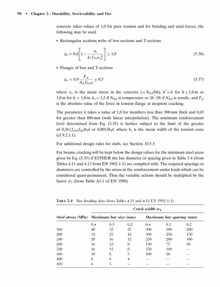
concrete takes values of 1,0 for pure tension and for bending and axial forces, the
following may be used
� Rectangular sections webs of box sections and T sections
kc ¼ 0,4 1 �c
k1 fct,effhh�
" #� 1,0 ð5:36Þ
� Flanges of box and T sections
kc ¼ 0,9Fcr
Act fct,eff� 0,5 ð5:37Þ
where c is the mean stress in the concrete (¼NEd/bh), h*¼ h for h� 1,0 m or
1,0 m for h4 1,0 m, k1¼ 1,5 if NEd is compressive or 2h*/3h if NEd is tensile, and Fct
is the absolute value of the force in tension flange at incipient cracking.
The parameter k takes a value of 1,0 for members less than 300 mm thick and 0,65
for greater than 800 mm (with linear interpolation). The minimum reinforcement
level determined from Eq. (5.35) is further subject to the limit of the greater
of 0,26 ( fctm/fyk)btd or 0,0013btd, where bt is the mean width of the tension zone
(cl 9.2.1.1).
For additional design rules for slabs, see Section 10.5.3.
For beams, cracking will be kept below the design values for the minimum steel areas
given by Eq. (5.35) if EITHER the bar diameter or spacing given in Table 5.4 (from
Tables 4.11 and 4.12 from EN 1992-1-1) are complied with. The required spacings or
diameters are controlled by the stress in the reinforcement under loads which can be
considered quasi-permanent. Thus the variable actions should be multiplied by the
factor 2 (from Table A1.1 of EN 1990)
TABLE 5.4 Bar detailing data (from Tables 4.11 and 4.12 EN 1992-1-1).
Crack width wk
Steel stress (MPa) Maximum bar size (mm) Maximum bar spacing (mm)
0,4 0,3 0,2 0,4 0,3 0,2160 40 32 25 300 300 200200 32 25 16 300 250 150240 20 16 12 250 200 100280 16 12 8 150 75 50320 16 12 8 150 100 --360 10 8 5 100 50 --400 8 6 4 -- -- --450 6 5 -- -- -- --
90 � Chapter 5 / Durability, Serviceability and Fire

In reinforced concrete the maximum bar diameter may be modified as follows:
Bending (at least part of the section in compression)
�s ¼ ��sfct,eff
2,9
kchcr
2ðh� dÞð5:38Þ
tension,
�s ¼ ��sfct,eff
2,9
hcr
24ðh� dÞð5:39Þ
where ��s is the maximum bar diameter from Table 5.4, �s is the adjusted value, h is
the depth of the section, hcr is the depth of the tensile zone immediately prior to
cracking under quasi-permanent load combinations and kc is given by Eq. (5.36) or
Eq. (5.37). For beams of depth greater than 1 m, additional reinforcement must
be provided in the tensile zone. It should have a minimum value obtained from
Eq. (5.35) with k¼ 0,5 and s¼ fyk. The spacing and size of such bars may be
obtained from Table 5.4 assuming pure tension and a steel stress half of that used in
the assessment of the main tensile reinforcement.
EXAMPLE 5.3 Crack width calculations. Check design crack width for the beam of
Examples 5.1 and 5.2
The critical zone is at the support.
Determine the clear spacing between bars:
s ¼ ð370 � 2 � 45 � 4 � 40Þ=3 ¼ 40 mm
Limiting spacing for closely spaced bars is 5(cþ�/2)¼ 5(45þ 40/2)¼ 325 mm.
Bars are thus closely spaced, thus sr,max is given by Eq. (5.31),
sr,max ¼ 3,4cþ 0,425k1k2�=p,eff
k1¼ 0,8 (high bond ribbed bars)
k2¼ 0,5 (flexure)
Effective loading:
Permanent: 30 kN/m
Quasi-permanent: 0,3�40¼ 12 kN/m (assuming 2¼ 0,3)
MSd ¼ 42 � 42=2 ¼ 336 kNm,
From Example 5.2:
Icr ¼ 11,46 � 109 mm4; x ¼ 298 mm
s ¼ �eMsdðd� xÞ=Icr ¼ 12,5 � 366 � 106� ð635 � 298Þ=11,46 � 109
¼ 135 MPa:
Ac,eff ¼ 2,5 ðh� dÞb ¼ 2,5ð700 � 635Þ370 ¼ 60125 mm2:
Concrete Design � 91

subject to the limits:
bðh� xÞ=3 ¼ 370ð700 � 298Þ=3 ¼ 49580 mm2
bh=2 ¼ 370 � 700=2 ¼ 129500 mm2
Thus Ac,eff should be taken as 49580 mm2
As ¼ 5026 mm2;
r ¼ As=Ac,eff ¼ 5026=49580 ¼ 0,101
� ¼ 40 mm, c ¼ 45 mm
Thus from Eq. (5.31),
sr,max ¼ 3,4 � 45þ 0,425 � 0,8 � 0,5 � 40=0,101 ¼ 220 mm
Determination of "sm� "cm (from Eq. (5.32)):
fct,eff may be taken as fctm¼ 0,3� fck(2/3)
¼ 2,56 MPa
Duration factor k1:
Conservatively assume long term loading, i.e. kt¼ 0,4, so from Eq. (5.32)
"sm � "cm ¼s � ktðfct,eff=p,effÞ 1 þ �e p,eff
�Es
¼135 � 0,4ð2,56=0,101Þ 1þ 12,5 � 0,101ð Þ
200 � 103¼ 653 � 10�6
Limiting value is given by 0,6s/Es¼ 0,6�135/200�103¼ 405�10�6
Thus, the value of "sm� "cm to be used is 653�10�6.
Determine wk from Eq. (5.31)
wk ¼ sr,max ð "sm � "cmÞ¼ 220 � 653 � 10�6
¼ 0,144 mm
This is below the limit of 0,3 mm, and therefore acceptable.
If the whole of the transient load is considered as permanent, then MSd¼ 560 kNm;
s ¼ 206 MPa; "sm� "cm¼ 1008 mstrain; wk¼ 0,22 mm (this is still satisfactory).
EXAMPLE 5.4 Bar spacing rules. The data are as before.
Determination of reinforcement stress s:
Effective loading:
Permanent: 30 kN/m
Quasi-permanent: 0,3�40¼ 12 kN/m (assuming 2¼ 0,3)
MSd ¼ 42 � 42=2 ¼ 336 kNm,
92 � Chapter 5 / Durability, Serviceability and Fire

From Example 5.2:
Icr ¼ 11,46 � 109 mm4; x ¼ 298 mm
s ¼ �eMsdðd� xÞ=Icr ¼ 12,5 � 366 � 106� ð635 � 298Þ=11,46 � 109
¼ 135 MPa:
Using the lowest value in Table 5.4 of s¼ 160 MPa, the maximum bar spacing for
wk¼ 0,3 is 300 mm. This is clearly satisfied as there are four bars in a total width of
370 mm.
The maximum bar size allowed (before modification) is 32 mm.
Use Eq. (5.38) for sections in flexure to determine the modified bar diameter:
��s ¼ 32 (from Table 5.4)
fct,eff:
This may be taken as fctm ¼ 0,3� f 2=3ck ¼ 2,56 MPa
The depth of the tensile zone at incipient cracking, hcr:
From Example 5.2, The depth of the uncracked neutral axis is 385 mm,
so, hcr¼ h� x¼ 700� 385¼ 315 mm.
Use Eq. (5.36) to determine kc:
As there is no applied axial force, c¼ 0, thus kc reduces to a value of 0,4.
So using (5.38)
�s ¼ ��sfct,eff
2,9kc hcr
2ðh� dÞ
¼ 322,56
2,9
0,4 � 315
2ð700 � 635Þ¼ 27,4 mm
Note in this case the modification factor produces a reduced bar diameter.
Interpolating between values of s of 200 and 240 from Table 5.4 gives a bar spacing
of around 240 mm. The actual is well below this. However, as EITHER the bar
diameter rules OR bar spacing rules need be satisfied, the design is satisfactory.
Note, a further example on crack width calculations is given in Example 11.5.
5.3 FIREDesign for fire is required, where applicable, in order to ensure any structure is
capable of withstanding the accidental effects of exposure from high temperatures
caused by the occurrence of fire. Although all multi-storey structures are required to
be checked for such effects, single storey structures may only need evaluating to
ensure the structure does not collapse outside its effective boundary. All building
structures need to be designed to ensure that evacuation of persons can be carried
out safely and that the fire can be fought with no ill-effects to the fire fighters
Concrete Design � 93
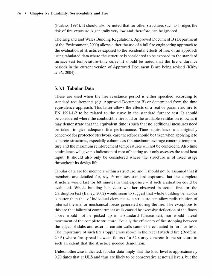
(Purkiss, 1996). It should also be noted that for other structures such as bridges the
risk of fire exposure is generally very low and therefore can be ignored.
The England and Wales Building Regulations, Approved Document B (Department
of the Environment, 2000) allows either the use of a full fire engineering approach to
the evaluation of structures exposed to the accidental effects of fire, or an approach
using tabulated data where the structure is considered to be exposed to the standard
furnace test temperature–time curve. It should be noted that the fire endurance
periods in the current version of Approved Document B are being revised (Kirby
et al., 2004).
5.3.1 Tabular Data
These are used when the fire resistance period is either specified according to
standard requirements (e.g. Approved Document B) or determined from the time
equivalence approach. This latter allows the effects of a real or parametric fire to
EN 1991-1-2 to be related to the curve in the standard furnace test. It should
be considered where the combustible fire load or the available ventilation is low as it
may demonstrate that the equivalent time is such that no additional measures need
be taken to give adequate fire performance. Time equivalence was originally
conceived for protected steelwork, care therefore should be taken when applying it to
concrete structures, especially columns as the maximum average concrete tempera-
ture and the maximum reinforcement temperatures will not be coincident. Also time
equivalence will give no indication of rate of heating as it only assesses the total heat
input. It should also only be considered where the structure is of fixed usage
throughout its design life.
Tabular data are for members within a structure, and it should not be assumed that if
members are detailed for, say, 60 minutes standard exposure that the complete
structure would last for 60 minutes in that exposure – if such a situation could be
evaluated. Whole building behaviour whether observed in actual fires or the
Cardington test (Bailey, 2002) would seem to suggest that whole building behaviour
is better than that of individual elements as a structure can allow redistribution of
internal thermal or mechanical forces generated during the fire. The exceptions to
this are that failure of compartment walls caused by excessive deflection of the floors
above would not be picked up in a standard furnace test, nor would lateral
movement of the complete structure. Equally the efficiency of fire stopping between
the edges of slabs and external curtain walls cannot be evaluated in furnace tests.
The importance of such fire stopping was shown in the recent Madrid fire (Redfern,
2005) where fire spread between floors of a 32 storey concrete frame structure to
such an extent that the structure needed demolition.
Unless otherwise indicated, tabular data imply that the load level is approximately
0,70 times that at ULS and thus are likely to be conservative at not all levels, but the
94 � Chapter 5 / Durability, Serviceability and Fire

variable load may be present during a fire other than in the extremely early period
during evacuation when any temperature rise within the concrete will be very low.
This is recognized in EN 1990 where a factor is applied to variable loading in the
calculation approach. EN 1992-1-2 does give a procedure whereby the critical
temperature and resultant axis distance can be modified for lower load levels (cl 5.2).
The critical temperatures �cr for a load level of 0,7 are taken as 5008C for reinforcing
steel, 4008C for prestressing in the form of bars, and 3508C for strand or wire. This
means that for bar prestressing, the tabulated values of the axis distance, a, should be
increased by 10 mm, and for strand or wires by 15 mm.
The major departure from current practice is that EN 1992-1-2 uses axis distance not
covered to reinforcement. This is actually more scientifically correct as it is observed
in computer-based heat transfer calculations that the temperatures at the centre of a
reinforcing bar are identical to that at the same position in plain concrete (Ehm,
1967, quoted in Hertz, 1981). Becker et al. (1974) indicate this is reasonable up to a
reinforcement area of 4 per cent of the gross section. Where the reinforcement is in
more than one layer, the weighted mean axis distance is used. The axis distance used
for any bar is the least of that to any fire exposed face. Rather than cover each type
of structural element, it is only proposed to cover those elements where
interpretation of the Code is required. Note in this section, all Table and clause
references are to EN 1992-1-2.
5.3.1.1 Columns
The Code provides two methods denoted A and B.
� Method A:
This was developed from an empirical procedure originally proposed by
Dortreppe and Franssen (undated). It can only be used under the following
recommended limits:
� Effective length l0,fi� 3 m, where l0,fi is taken as l0 (the effective length at
ambient) subject to the condition that if the standard exposure is greater
than 30 minutes, then l0,fi is taken as 0,5l for intermediate floors and
0,5l� l0,fi� 0,7l for the upper floor (l is the height of the column between
centre lines).� Eccentricity of load, e, defined as M0Ed,fi/N0Ed,fi, should be less than emax which
has a recommended value of the lesser of 0,15h or b (although the code does
suggest an upper limit of 04h or b). M0Ed,fi and N0Ed,fi are the first order moment
and axial force in the fire limit state.� Maximum reinforcement As should not exceed 0,4Ac.
NOTE: The design values of section size and cover given in Table 5.2a of EN 1992-
1-2 are for a value of �cc of 1,00. Thus if a value of 0,85 is adopted (as is likely in
the UK), the formula attached to the Table MUST be used. This gives the value of
Concrete Design � 95

the fire resistance R as
R ¼ 120R�fi þRa þRl þRb þRn
120
� �1,8
ð5:40Þ
where the correction factor R�fi for load level �fi and �cc is given by
R�fi ¼83 1,00 � �fi1 þ !
ð0,85=�ccÞ þ !
� �ð5:41Þ
where �fi is defined as NEd.fi/NRd (i.e. the ratio of the axial load in the fire limit
state to the design resistance at ambient) and ! is the mechanical reinforcement
ratio (¼As fyd/Ac fcd¼ (As fyk/�s)/(Ac fck/�c),
the correction factor Ra for axis distance a ( 25� a� 80 mm),
Ra ¼ 1,6ða� 30Þ ð5:42Þ
the correction factor Rl for effective length l0,fi,
Rl ¼ 9,60 5 � l0,fi
�ð5:43Þ
the correction factor Rb for a parametric width b0 (200� b0 � 450 mm),
Rb ¼ 0,9b0 ð5:44Þ
where for a circular column b0 is the diameter, and for a rectangular column b0 is
given by
b0 ¼2Ac
bþhð5:45Þ
subject to the limit that h� 1,5b.
� Method B:
The background to Method B is given in Dortreppe, Franssen and Vanderzeypen
(1999).
This is covered at a basic level in Table 5.2b with more detailed tables in Annex C
of EN 1992-1-2.
The tables operate in terms of a load level n defined as
n ¼NoEd,fi
0,7 Ac fcd þ As fyd
� ð5:46Þ
and the mechanical reinforcement ratio !.
Table 5.2b also has the restrictions that e/b� 0,25 (subject to a maximum value of e
of 100 mm) and the slenderness ratio in the fire limit state �fi5 30.
96 � Chapter 5 / Durability, Serviceability and Fire
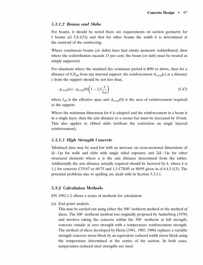
5.3.1.2 Beams and Slabs
For beams, it should be noted there are requirements on section geometry for
I beams (cl 5.6.1(5)) and that for other beams the width b is determined at
the centroid of the reinforcing.
Where continuous beams (or slabs) have had elastic moments redistributed, then
where the redistribution exceeds 15 per cent, the beam (or slab) must be treated as
simply supported.
For situations where the standard fire resistance period is R90 or above, then for a
distance of 0,3leff from any internal support, the reinforcement As,req(x) at a distance
x from the support should be not less than,
As,reqðxÞ¼ As,reqð0Þ 1 � 2,5x
leff
� �ð5:47Þ
where leff is the effective span and As,req(0) is the area of reinforcement required
at the support.
Where the minimum dimension for b is adopted and the reinforcement in a beam is
in a single layer, then the axis distance to a corner bar must be increased by 10 mm.
This also applies to ribbed slabs (without the restriction on single layered
reinforcement).
5.3.1.3 High Strength Concrete
Tabulated data may be used but with an increase on cross-sectional dimensions of
(k�1)a for walls and slabs with single sided exposure and 2(k�1)a for other
structural elements where a is the axis distance determined from the tables.
Additionally the axis distance actually required should be factored by k, where k is
1,1 for concrete C55/67 or 60/75 and 1,3 C70/85 or 80/95 given in cl 6.4.3.1(3). The
potential problems due to spalling are dealt with in Section 5.3.3.1.
5.3.2 Calculation Methods
EN 1992-1-2 allows a series of methods for calculation:
(a) End point analysis.
This may be carried out using either the 5008 isotherm method or the method of
slices. The 5008 isotherm method was originally proposed by Anderberg (1978)
and involves taking the concrete within the 5008 isotherm at full strength,
concrete outside at zero strength with a temperature reinforcement strength.
The method of slices developed by Hertz (1981, 1985, 1988) replaces a variable
strength concrete stress block by an equivalent reduced width stress block using
the temperature determined at the centre of the section. In both cases,
temperature-reduced steel strengths are used.
Concrete Design � 97
(b) Full analysis.
An analysis using acceptable materials models incorporating transient strain
for the concrete can be used. This is a specialist approach and involves the
use of Finite Element techniques for both the determination of the tempera-
ture field within the structure and the resultant stresses, strains and
deformations.
Design methods by calculation will not be covered in this text and reference should
be made to Purkiss (1996).
5.3.3 Additional Comments
5.3.3.1. Spalling
Spalling occurs in one of two main forms in a fire. The first is explosive spalling
which occurs very early in a fire and is likely to lead to loss of cover to the
main reinforcing and hence to more rapid rises in temperature and resultant
strength loss leading to reduced fire performance. The second form is known
as sloughing whereby the concrete gradually comes away due to loss of effective
bond and strength loss. This mode tends to occur toward the end of a fire and
is rarely critical. It should be noted that although there can be severe spalling
in a fire, the structure may still be capable of withstanding the effects of the fire
without collapse. This was demonstrated in the fire test on the large frame structure
at Cardington (Bailey, 2002).
The exact mechanism of explosive spalling is still not completely understood,
although Connolly (1995, 1997) has indicated that there is unlikely to be one
single mechanism. High Strength Concrete (HSC) and Self-Compacting
Concrete (SCC) may give potentially worse problems in fire due to spalling
than normal strength concrete due to their extremely low porosity. These
concretes should both have polypropylene fibres with a dosage rate of 2 per
cent included in the mix (EN 1992-1-2; Persson, 2003). The following factors
affecting spalling have been identified (Malhotra, 1984; Connolly, 1995 and
1997):
� Moisture content
A concrete with a high moisture content is more likely to spall, since
one of the possible mechanisms of spalling is due to the build up of
high vapour pressures by moisture clog in the element. The blanket limit
of a moisture content of 3 per cent, below which EN 1991-1-2 indicates
spalling will not occur, should be questioned. The original proposal
based on work by Meyer-Ottens (1975) also suggested stress limits. If
the permeability is high then a high moisture content may not cause
problems.
98 � Chapter 5 / Durability, Serviceability and Fire
� Concrete porosity
A more porous concrete will allow the dissipation of vapour pressure, and
thus relieve any build up within the section. A reminder needs to be made of
the relationship between porosity and strength, in that the lower the porosity,
the higher the strength. However, it must be pointed out that a porous
concrete will give a poor performance with respect to durability.
� Stress conditions
From evidence of fire tests and observations in fires, it has been noted that
spalling is likely to be more severe in areas where the concrete cross section is
in compression, i.e. areas of hogging moments in beams or slabs, or in
columns. This can partly be explained by the fact that in areas of compressive
stresses, cracks cannot open up to relieve internal pressures. This does not
mean that spalling cannot occur in areas of sagging moments where tensile
cracks exist, since it is possible that pressure build up will still occur as in
general tension cracks are discrete and not part of a continuum.
� Aggregate type
Historically, the evidence available appeared to suggest that the aggregate
most likely to give spalling is siliceous aggregate, with limestone producing
less spalling and lightweight concrete the least. This is likely to be linked to
the basic porosity of the aggregate in that siliceous aggregate is impermeable
compared to the others and that moisture transport has to occur through the
mortar matrix. However, there is now some evidence that limestone and
lightweight aggregates may give problems, especially in younger concretes as
the pore structure provides convenient reservoir storage for free water
(Connolly, 1995).
� Section profile and cover
There is some evidence to suggest that sharp profiles will produce more
spalling than rounded or chamfered edges. Spalling is also exacerbated in thin
sections, partly since the depth of spalling is a greater proportion of the
section dimension and hence proportionally worse, and partly due to the fact
that there is less of a cool reservoir for any moisture to migrate towards.
High covers are also likely to produce greater amounts of spalling as the
concrete is not restrained in a triaxial state of stress in the surface layers. Thus
design codes frequently place restrictions when high covers are needed at high
fire resistance periods in order to maintain low temperatures in the
reinforcing. EN 1992-1-2 indicates that for axis distances of greater than
70 mm a mesh with wires of at least 4 mm and spacing of 100 mm should be
provided at the surface (cl 4.5.2(2)). It should, however, be noted that tests
have shown that even with high covers such additional reinforcement is not
absolutely necessary to give fire resistance periods of up to 4 hours (Lawson,
1985).
Concrete Design � 99

� Heating Rate
The higher the heating rate, the less chance the pore water has migrated from
the outside hot layers to the relatively cooler central layers of a member
(Shorter and Harmathy, 1965). Thus the rate of heat given off by the fire is
critical for an assessment of the likelihood of spalling. A hydrocarbon-type
fire will therefore be worse than a cellulosic-type fire as the rate of heat
release is higher.
5.3.3.2 Shear and Bond
For simply supported or continuous reinforced concrete, construction shear has
rarely been observed as a problem. For large prestressed concrete beams, Bobrowski
and Bardhan-Roy (1969) indicated that a potentially critical section for shear was
between 0,15L and 0,2L from the support where L is the span. This is due to the
moments induced in the section by the prestress itself which will not be constant
along the length of the beam owing to the varying profile of the tendons. Shear was
thought to be potentially critical in conventional precast prestressed concrete floor
units as shear resistance is provided entirely by the tendons which are however
placed close to the fire exposed face of the units. However work reported by Acker
(2003/2004) and Lennon (2003) indicates that this appears not to be the case,
provided the precast units are constrained to act as a diaphragm by being tied
together by reinforcement in the plane of the floor. The tests reported by Lennon
which were under a compartment fire regime rather than the standard furnace
curve also indicated there was no spalling and that the load carrying capacity was
satisfactory up to a time-equivalent of around 60 minutes. The test results for load
carrying capacity should not be extrapolated beyond this point. Bond is generally not
a problem even though bond strengths are severely reduced in a fire.
5.3.3.3 Detailing
It should be self-evident that the prime factor controlling fire performance is axis
distance to the reinforcement which in practical terms means any specified cover
must be guaranteed. Clark et al. (1997) indicated that from surveys carried out,
15 per cent of the measured covers failed to achieve their minimum values. Although
no indication was given on the magnitude of such failure, it is clear that there could
be problems with fire performance. A parametric study by Purkiss and Du (2000)
indicates that for columns, variations in cover have little effect on fire performance.
For the top reinforcement in slabs or beams (other than that adjacent to the fire
exposed surface), there will be little effect on the fire performance. However, for the
bottom reinforcement in beams or slabs to have insufficient cover is potentially very
dangerous as the fire endurance will be severely compromised. Purkiss, Claridge and
Durkin (1989) noted in a simple simulation on slab behaviour in fire that variations
in cover was the most significant variable for changes in fire performance. If there is
100 � Chapter 5 / Durability, Serviceability and Fire

adequate top reinforcement correctly detailed, then some moment transfer could
occur. It should be admitted that the tabular data are likely to be conservative,
provided the points noted below are considered. Lennon (2004a,b) has indicated
that the data in BS 8110 were set below test results. This situation is also likely for
EN 1992-1-2 as the data are not dissimilar. It should be noted that the only column
test data available then were for columns heated on four sides under axial loads.
Thus the margin of safety for edge or corner columns heated on two or three sides
with a moment gradient is unquantifiable. However, the level of safety will be
reduced, should the correct covers not be achieved on site. There are, however, two
additional issues which should be raised:
(1) It was demonstrated in the Cardington tests, both on the concrete and steel
frame, that damage to the structure also occurred during the cooling phase
owing to the effects of contraction on a tied structure.
(2) The relevance of the BS 476 Part 20 (or similar) curve must be questioned for
modern buildings. It has often been suggested with no hard evidence that the
heating phase of the standard curve is equivalent to the heating curve for a
moderate fire in an office-type environment. This might just have been feasible
where the contents were totally, or almost totally, cellulosic.
It is not true for modern offices where the contents are plastic (or hydrocarbon
based). Hydrocarbon fires are of shorter duration but have a higher rate of heat
release. This means that whilst it is possible that the critical temperatures reached
in concrete elements (or structures) are lower, the effect on spalling will be to
potentially increase its occurrence and severity owing to the higher thermal gradients
close to the surface.
The Cardington Test also showed the importance of ensuring the concrete design
strength is adhered to during construction, as concrete strengths increased for
whatever reason can lead to an increased probability of spalling. Thus any
consideration of enhanced strengths over design values must be cleared by the
designer in order to assess any possible detrimental effects. It is possible therefore
that the designer may need to specify both minimum and maximum strengths for any
concrete that could potentially be exposed to fire.
5.3.3.4 Whole Building Behaviour
The one fire test on the concrete frame at the large test facility at Cardington
reported by Bailey (2002) showed up some interesting features. The structure was
tested at an age of around three and a half years. The first was that the columns cast
from high strength concrete did not spall in spite of a moisture content of per cent,
although the dosage of polypropylene fibres of 2,7 kg/m3 was higher than the
recommended value of 2 kg/m3 in EN 1992-1-2. There was some splitting on the
arises of the column although this was likely to have been caused late in the test.
Concrete Design � 101
The slab, however, underwent substantial spalling, the reasons for this were the use
of a flint-type aggregate, the moisture content of per cent, a concrete cube strength
of 61 MPa at 28 days (cylinder strength of approximately 50 MPa) compared with the
design mix strength class C37.
However before extrapolating the results from Cardington to other structures, a
number of points need to be noted (Chana and Price, 2003). The first is that the
original emphasis on the project was to investigate optimization of the construction
process. The second was that the high moisture contents were due to the structure
being in a relatively cool unventilated enclosure where drying would have been
at the very least slow. The third is that the structure was of flat slab construction
with steel cross bracing. This means that the lateral movements noted during the
test would almost certainly have been less had the structure had in situ concrete
lift shafts or stair wells, but the increased restraint may have exacerbated the spalling
of the slab. The movements noted were enough to have buckled the steel flats in
the bracing.
REFERENCES AND FURTHER READING
Acker, A. Van, (2003/2004) Shear Resistance of prestressed hollow core floors exposed to fire,
Structural Concrete, Journal of the fib, 2, June 2003.
Anderberg, Y. (1978) Analytical Fire Engineering design of reinforced concrete structures based on
real fire characteristics, Proceedings of the Eighth Congress of the Federation Internationale de la
Precontrainte, London 1978, Concrete Society, 112–123.
Bailey, C.J. (2002) Holistic Behaviour of Concrete Buildings in Fire, Proceedings of the Institution of
Civil Engineers, Buildings and Structures, 152, 199–212.
Bamforth, P.B. (2004) Enhancing Concrete Durability, Technical Report 61, Concrete Society.
Becker, J., Bizri, H. and Bresler, B. (1974) FIRES-T2 A Computer Program for the Fire Response of
Structures-Thermal, Report No UCB-FRG 74-1, Department of Civil Engineering, University of
Berkeley, California.
Beeby, A.W. (1978) Corrosion of reinforcing steel in concrete and its relation to cracking, Structural
Engineer, 56A(3), 77–81.
Beeby, A.W. (1979) The prediction of crack widths in hardened concrete, Structural Engineer,
57A(1), 9–17.
Beeby, A.W., Scott, R.H. and Jones, A.E.K. (2005) Revised Code provisions for long-term
deflection calculations, Proceedings of the Institution of Civil Engineers, Structures and Buildings,
158, 71–75.
Bobrowski, J. and Bardhan-Roy, B.K. (1969) A method of calculating the ultimate strength of
reinforced and prestressed concrete beams in combined flexure and shear, Structural Engineer,
47, 3–15.
BRE (2004) Alkali-Silica Reaction in Concrete (Parts 1–4), Building Research Establishment,
Garston.
BS EN 206-1:2000 Concrete – Part 1: Specification, performance, production and conformity,
British Standards Institution/ Comite European de Normalisation.
Chana, P. and Price, W. (2003) The Cardington Fire Test, Concrete, 37(1), 28, 30–33.
Clark, L.A., Shammas-Toma, M.G.K., Seymour, E., Pallett, P.F. and Marsh, B.K. (1997) How can we
get the cover we need? Structural Engineer, 75(17), 289–296.
Connolly, R.J (1995) The Spalling of Concrete in Fires, PhD Thesis, University of Aston.
102 � Chapter 5 / Durability, Serviceability and Fire

Connolly, R.J. (1997) The spalling of concrete, Fire Engineers Journal, 38–40.
Dallard, P., Fitzpatrick, A.J., Flint, A., LeBourva, S., Ridstill Smith, R.M. and Willford, M. (2001)
The London Millennium Footbridge, Structural Engineer, 79(22), 17–33.
DOE (1991) Building Regulations: Approved Document B: Fire Safety (reissued 2000), Stationary
Office.
Dotreppe, J.C. and Franssen, J.M. (undated) Fire Attack on concrete Columns and Design Rules
under Fire Conditions, Proceedings of a Symposium on Computational and Experimental Methods
in Mechanical and Thermal Engineering [100th Anniversary of the Laboratory of Machines and
Machine Construction, Department of Mechanical and Thermal Engineering], Universeit Gent,
unpaginated.
Dotreppe, J.C., Franssen, J.M., and Vanderzeypen, Y. (1999) Calculation Method for Design of
Reinforced Concrete Columns under fire Conditions, American Concrete Institute, Structural
Journal, 96(1), 9–18.
Dunster, A.M. and Crammond, N.J. (2003) Deterioration of cement-based building materials:
Lessons learnt, Information Paper IP 4/03, Building Research Establishment.
Ehm, H (1967) Ein Betrag zur reichnerischung Bemessung von brandbeanspruchten balkenartigen
Stahlbetonbauteilen, Technische Hochshule Braunschweig.
Henderson, N.A., Baldwin, N.J.R., McKibbins, L.D., Winsor, D.S. and Shanghavi, H.B. (2002)
Concrete technology for cast in-situ foundations, Report 569, Construction Industry Research
and Information Association.
Hertz, K (1981) Simple Temperature Calculations of Fire Exposed Concrete Structures, Report No
159, Institute of Building Design, Technical University of Denmark.
Hertz, K (1985) Analyses of Prestressed Concrete Structures exposed to Fire, Report No 174,
Institute of Building Design, Technical University of Denmark.
Hertz, K (1988) Stress Distribution Factors (2nd Ed), Report No. 190, Institute of Building Design,
Technical University of Denmark.
Johnson, R.P. and Anderson, D. (2004) Designers’ Guide to EN 1994-1-1. Eurocode 4; Design of
Composite steel and concrete structures, Part 1.1: General Rules and Rules for buildings,
Thomas Telford.
Kirby, B.R., Newman, G.M., Butterworth, N., Pagan, J. and English, C (2004) A new approach to
specifying fire resistance periods. Structural Engineer, 82(12), 34–37.
Lawson, R.M. (1985) Fire resistance of Ribbed Concrete floors, Report No 107, Construction
Industry Research and Information Association, London.
Lennon, T. (2003) Precast Hollowcore slabs in Fire, Information Paper IP 5/03, Building Research
Establishment.
Lennon, T. (2004a) Fire safety of concrete structures: Background to BS 8110 fire design, Report
BR 468, Building Research Establishment.
Lennon, T. (2004b) Fire safety of concrete structures, Structural Engineer, 82(6), 22–24
Malhotra, H.L. (1984) Spalling of Concrete in Fires, Technical Note No 118, Construction Industry
Research and Information Association, London.
Meyer-Ottens, C (1975) Zur Frage der Abplatzungen an Bautelien aus Beton bei Brandbean-
spruchungen, Deutsche Ausschuß fur Stahlbeton, Heft 248.
Page, C.L. and Treadaway, K.W.J. (1982) Aspects of the electrochemistry of steel in concrete,
Nature, 297(5862), 109–115.
Persson, B. (2003) Self-compacting concrete at fire temperatures. Report No TVBM 3110, Lund
Institute of Technology, Lund University, Denmark.
Purkiss, J.A (1996) Fire Safety Engineering Design of Structures, Butterworth-Heinemann.
Purkiss, J.A. and Du, Y. (2000) A parametric study of factors affecting the fire performance of
reinforced concrete columns, In Concrete Communication Conference 2000 (10th Annual BCA
Conference), Birmingham University 29–30th June 2000, pp. 267–275.
Purkiss, J.A., Claridge, S.L. and Durkin, P.S. (1989) Calibration of simple methods of calculating
the fire resistance of flexural reinforced concrete members, Fire Safety Journal, 15, 245–263.
Concrete Design � 103

Shorter, G.W. and Harmathy, T.Z. (1965) Moisture clog spalling. Proceedings of the Institution
of Civil Engineers, 20, 75–90.
Redfern, B. (2005) Lack of fire stops blamed for speed of Madrid tower inferno, New Civil
Engineer, 17 February, 5–7.
Taumasite Experts Group (1999) The Structural implications of the taumasite form of sulfate
attack, Structural Engineer, 77(4), 10–11.
104 � Chapter 5 / Durability, Serviceability and Fire

C h a p t e r 6 / Reinforced Concrete Beamsin Flexure
This chapter deals with the flexural design of both rectangular and flanged
reinforced concrete beams.
Clause 6.1 of EN 1992-1-2 lays down the general principles which are:
Plane sections remain plane
The strain in the reinforcing steel is equal to that of the surrounding concrete
The tensile strength of the concrete is ignored
The stresses in the concrete are derived from
(a) Full stress–strain curve (Fig. 6.1 (a))
(b) Parabolic–rectangular stress block (Fig. 6.1 (b))(c) Equivalent rectangular stress block (Fig. 6.1 (c)).
The stresses in the reinforcement are derived from the relationship shown in
Fig. 6.2
The compressive strain of the concrete is limited to ecu2 or ecu3 as appropriate.
Note, the values of "cu2 or "cu3 are given in Table 3.1 of EN 1991-1-2. Moss and
Webster (2004) indicate there is little difference between whichever of the three
stress blocks are chosen for pure flexural design. As the rectangular stress block
leads to a very simple approach to design, it is the assumption which will be used
in this chapter.
At relatively low values of applied bending moment, beams are designed with tensile
reinforcement only, and are said to be singly reinforced, and those requiring tensile
and compression reinforcement to resist much higher applied loading are denoted as
doubly reinforced. In addition, the shear induced by the applied loading also needs to
be resisted. This resistance is commonly provided by the use of shear links, although
other approaches such as bent-up bars or a combination of bent-up bars and shear
links may be used. Even if a beam is singly reinforced, the shear links will need
supporting in the compression zone by bars at each corner of any links. These bars
provide anchorage for the link and enable the total reinforcement to be assembled as

sc
fcm
0,4 fcm
sc
fck
fcd
ec
ec
Ecm
ec1
(a) Full stress–strain curve
(b) Parabolic – rectangular stress block
ecu1
ec2 ecu2
x Fc
hfcd
Neutral axis
(c) Equivalent rectangular stress block
lx
FIGURE 6.1 Possibleconcrete stress blocks
efyd/E
s
fyd = fyk/gs
FIGURE 6.2 Reinforcement stress–strainbehaviour
106 � Chapter 6 / Reinforced Concrete Beams in Flexure

a reinforcing cage. In order to provide the cage with stability and, where the cage
is prefabricated, to enable it to be lifted into position, the top steel should be not
less than 16 mm high yield steel. A typical beam detail is given in Fig. 6.3. Where
there is compression steel, the links have a secondary function which is to restrain
the compression steel to prevent it from buckling.
6.1 BEHAVIOUR OF BEAMS IN FLEXUREA set of theoretical moment-curvature diagrams are plotted in Fig. 6.4, albeit with a
slightly different concrete stress–strain curve to that in EN 1992-1-1 and a
reinforcement yield stress of 460 MPa. A similar set of diagrams would be
obtained were the stress–strain curve in EN 1992-1-1 and a yield stress of
500 MPa to be used.
If Fig. 6.4 be examined, there appears two distinct patterns of behaviour. The first
pattern is where there is a considerable increase in curvature after the attainment of
the maximum moment and where the behaviour exhibits a characteristic close to
elastic–perfectly plastic behaviour. The second type of behaviour is where failure
occurs as the maximum moment is achieved with no subsequent ductility. The first
type of behaviour clearly allows a large degree of rotation after yield, albeit
accompanied by severe and increased cracking and deflection. This behaviour is
exhibited by sections defined as under-reinforced, where the reinforcement yields
before the concrete reaches its maximum strain capacity. The behaviour with no
post-yield plateau is given by an over-reinforced section where the steel remains
elastic and the concrete reaches its maximum strain before the steel yields. An over-
reinforced section gives no prior warning of distress and therefore tends to be
considered as unsafe. A section at which the steel yields at the same time as the
concrete reaches its maximum strain is known as a balanced section.
At balance, the steel strain "yd is given by
"yd ¼fyk
Es�s¼
fyk
200 � 103 � 1,15¼
fyk
0,23 � 106ð6:1Þ
Compression reinforcement
Tension reinforcement
ElevationLinks
Section
FIGURE 6.3 Arrangement of reinforcement in a beam
Concrete Design � 107
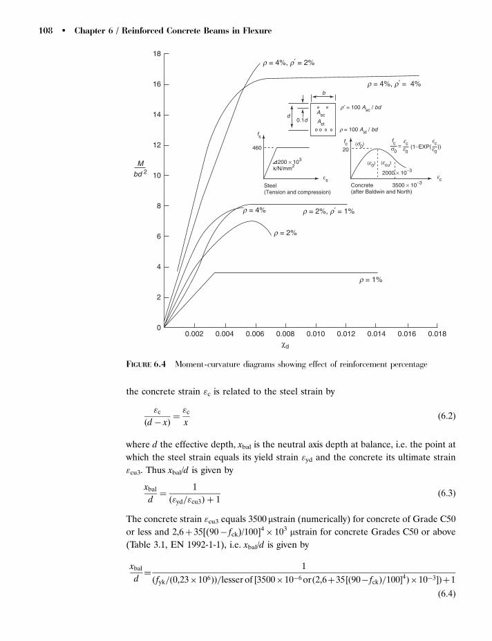
the concrete strain "c is related to the steel strain by
"c
ðd� xÞ¼"c
xð6:2Þ
where d the effective depth, xbal is the neutral axis depth at balance, i.e. the point at
which the steel strain equals its yield strain "yd and the concrete its ultimate strain
"cu3. Thus xbal/d is given by
xbal
d¼
1
ð"yd="cu3Þ þ 1ð6:3Þ
The concrete strain "cu3 equals 3500 mstrain (numerically) for concrete of Grade C50
or less and 2,6þ 35[(90� fck)/100]4� 103 mstrain for concrete Grades C50 or above
(Table 3.1, EN 1992-1-1), i.e. xbal/d is given by
xbal
d¼
1
ðfyk=ð0,23�106ÞÞ=lesser of ½3500�10�6 orð2,6þ35 ½ð90� fckÞ=100�4Þ�10�3�Þþ1
ð6:4Þ
χd
r = 1%
r = 2%
460 20
Steel(Tension and compression)
200 × 103
k/N/mm2
fsfc fc
dAsc
Ast
b
(s0)s0
(e0)
e0
ec
ec
(ecu)
0.1d
Concrete(after Baldwin and North)
3500 × 10−3
2000 × 10−3
r = 4% r = 2%, r′ = 1%
r = 4%, r′ = 2%
r = 4%, r′ = 4%
00.002 0.004 0.006 0.008 0.010 0.012 0.014 0.016 0.018
2
4
6
8
10
12
14
16
18
Mbd 2 εs
r′ = 100 Asc / bd
r = 100 Ast / bd
= (1−EXP( ))ece0
FIGURE 6.4 Moment-curvature diagrams showing effect of reinforcement percentage
108 � Chapter 6 / Reinforced Concrete Beams in Flexure
For Grade C50 concrete (or below) Eq. (6.4) reduces to
xbal
d¼
1
ð fyk=ð0,23 � 106ÞÞð1=ð3500 � 10�6ÞÞ þ 1¼
1
ð fyk=805Þ þ 1ð6:5Þ
for fyk¼ 500 MPa, xbal/d¼ 0,617 and for fyk¼ 250 MPa, 0,763, respectively. In both
these cases the balanced neutral axis depth is higher than that allowed by cl 5.5 (4).
6.1.1 Limits on Neutral Axis Depth
Where plastic analysis has been used to determine the internal forces in a member,
such as slabs using yield line theory (Section 10.4), the limiting value of xu/d is
0,25 for concretes of Grade 50 or below and 0,15 for concrete grades higher than
C50 (cl 5.6.2 (2)). This is to ensure the section has sufficient ductility to allow the
formation and rotation of plastic hinges.
There are also restrictions placed on the rotations at internal supports for both
continuous beams and one-way spanning slabs (See Section 4.7).
Where an elastic analysis is used and the resultant moments redistributed to give
simulated plastic analysis (Section 4.7) there are also limits on the x/d ratio to ensure
ductility. These limits are
� for concrete of grade C50 or less
� � 0,44 þ 1,25 0,6 þ0,0014
"cu2
� �x
d� 0,7 ð6:6Þ
� for concrete above grade C50
� � 0,54 þ 1,25 0,6 þ0,0014
"cu2
� �x
d� 0,8 ð6:7Þ
where � is defined as the ratio of the redistributed moment to the moment before
redistribution. For concrete of grade C50 or less, "cu2¼ 0,0035, thus Eq. (6.7)
reduces to
� � 0,44 þ 1,25x
d� 0,7 ð6:8Þ
6.2 SINGLY REINFORCED SECTIONS
The forces acting on the section are shown in Fig. 6.5. The numerical value of
the resultant compression force Fc from the rectangular concrete stress block is
given by
Fc ¼��cc fck
�cð�xÞb ð6:9Þ
Concrete Design � 109
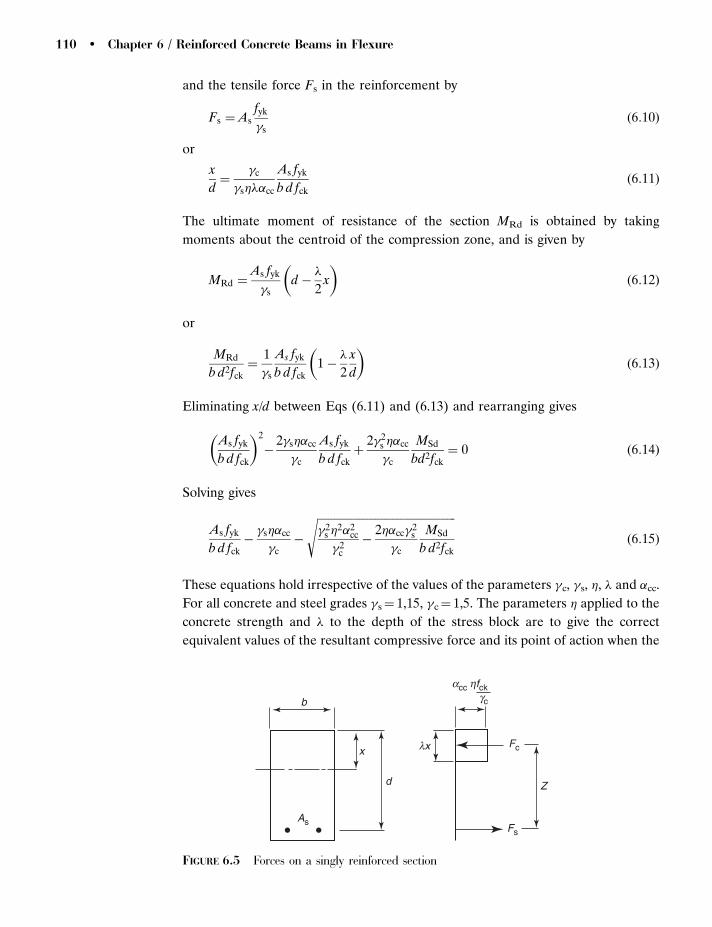
and the tensile force Fs in the reinforcement by
Fs ¼ Asfyk
�sð6:10Þ
or
x
d¼
�c
�s���cc
As fyk
b d fckð6:11Þ
The ultimate moment of resistance of the section MRd is obtained by taking
moments about the centroid of the compression zone, and is given by
MRd ¼As fyk
�sd�
�
2x
� �ð6:12Þ
or
MRd
b d2fck¼
1
�s
As fyk
b d fck1 �
�
2
x
d
� �ð6:13Þ
Eliminating x/d between Eqs (6.11) and (6.13) and rearranging gives
As fyk
b d fck
� �2
�2�s��cc
�c
As fyk
b d fckþ
2�2s ��cc
�c
MSd
bd2fck¼ 0 ð6:14Þ
Solving gives
As fyk
b d fck��s��cc
�c�
ffiffiffiffiffiffiffiffiffiffiffiffiffiffiffiffiffiffiffiffiffiffiffiffiffiffiffiffiffiffiffiffiffiffiffiffiffiffiffiffiffiffiffiffiffiffiffiffiffiffi�2
s �2�2
cc
�2c
�2��cc�2
s
�c
MSd
b d2fck
sð6:15Þ
These equations hold irrespective of the values of the parameters �c, �s, �, � and �cc.
For all concrete and steel grades �s¼ 1,15, �c¼ 1,5. The parameters � applied to the
concrete strength and � to the depth of the stress block are to give the correct
equivalent values of the resultant compressive force and its point of action when the
b
d
As
lx
acc hfck
Fc
Fs
Z
x
gc
FIGURE 6.5 Forces on a singly reinforced section
110 � Chapter 6 / Reinforced Concrete Beams in Flexure

rectangular stress block rather than the complete stress–strain curve is used. The
values of � are concrete strength dependant as the shape of the stress–strain curve
changes with concrete strength as the absolute value of ultimate strain in the
concrete decreases with strength and the strain at maximum stress increases with
strength. If the concrete grade is restricted to C50/60 or below, and � may be taken
as constant with �¼ 0,8 and �¼ 1,0, which allows Eq. (6.12) to (6.15) to be
simplified. For concrete grades higher than C50, it is not possible to perform this
operation as both � and � are dependant upon the concrete strength,
� ¼ 0,8 �fck � 50
400ð6:16Þ
and
� ¼ 1,0 �fck � 50
200ð6:17Þ
Equation (6.12) is independent of the value of �cc and becomes for Grade C50
or below,
MRd
b d2fck¼
1
1,15
As fyk
b d fck1 � 0,4
x
d
� �ð6:18Þ
The value of the coefficient acc which allows for long term effects on the compressive
strength should lie between 0,8 and 1,0 (cl 3.1.6 (1)P), with a recommendation that it
may be taken as 1,0. However, UK practice has conventionally taken a value of 0,85
for ULS design under ambient conditions. For any accidental limit state, such as fire,
the need to consider creep effects can be ignored and �cc set equal to 1.
It is therefore useful to derive flexural design equations for values of �cc of both 1,0
and 0,85, although it should be noted that all the ambient design examples for
reinforced concrete in this and subsequent chapters will be carried out with �cc of
0,85.
� For �cc¼ 0,85,
The neutral axis depth x/d is given by
x
d¼
1,5
1,15 � 1,0 � 0,8 � 0,85
As fyk
b d fck¼ 1,918
As fyk
b d fckð6:19Þ
Equation (6.14) reduces to
As fyk
b d fck
� �2
�1,15 � 2 � 0,85
1,5
As fyk
b d fckþ
1,152 � 2 � 0,85
1,5
MSd
bd2fck¼ 0 ð6:20Þ
Concrete Design � 111

which becomes
As fyk
b d fck
� �2
�1,303As fyk
b d fckþ 1,534
MSd
bd2fck¼ 0 ð6:21Þ
Solving gives (with a slight rounding of values)
As fyk
b d fck¼ 0,652 �
ffiffiffiffiffiffiffiffiffiffiffiffiffiffiffiffiffiffiffiffiffiffiffiffiffiffiffiffiffiffiffiffiffiffiffiffi0,425 � 1,5
MSd
bd2fck
sð6:22Þ
To determine Msd in terms of As, Eq. (6.19) may be substituted into Eq. (6.18)
to give
MRd
bd2fck¼ 0,87
As fyk
b d fck1 � 0,767
As fyk
b d fck
� �ð6:23Þ
� For �cc¼ 1,0,
x
d¼
1,5
1,15 � 1,0 � 0,8 � 1,0
As fyk
b d fck¼ 1,63
As fyk
b d fckð6:24Þ
Equation (6.14) becomes
As fyk
b d fck
� �2
�1,15 � 2 � 1,0
1,5
As fyk
b d fckþ
1,152 � 2 � 1,0
1,5
MSd
bd2fck¼ 0 ð6:25Þ
or
As fyk
b d fck
� �2
�1,533As fyk
b d fckþ 1,763
MSd
bd2fck¼ 0 ð6:26Þ
Solving gives
As fyk
b d fck¼ 0,767 �
ffiffiffiffiffiffiffiffiffiffiffiffiffiffiffiffiffiffiffiffiffiffiffiffiffiffiffiffiffiffiffiffiffiffiffiffiffiffiffi0,588 � 1,76
MSd
b d2fck
sð6:27Þ
To determine Msd in terms of As, Eq. (6.24) may be substituted into Eq. (6.18)
to give
MRd
b d2fck¼ 0,87
As fyk
b d fck1 � 0,652
As fyk
b d fck
� �ð6:28Þ
It is instructive to compare the effects of the two values of �cc. This is carried out in
Table 6.1. It will be observed that there is virtually no difference in the values of
As fyk/bdfck obtained using the two values of �cc, any such reductions are likely to be
112 � Chapter 6 / Reinforced Concrete Beams in Flexure

eliminated when the mechanical reinforcement ratio As fyk/bdfck is converted to
actual bar sizes. The main effect is that the higher value of �cc will give lower values
of x/d, hence a slightly higher moment capacity before compression reinforcement is
required.
For �cc¼ 0,85, the limiting moment a singly reinforced section can take is obtained
by substituting the maximum value of x/d from Eq. (6.8) into Eq. (6.19) to determine
the limiting value of As fyk/bdfck, and the coexistent value of MSd/bd2fck from
Eq. (6.21). A similar procedure may be adopted for �cc¼ 1,0 using Eqs (6.24) and
(6.28). The results of these calculations are given in Table 6.2.
EXAMPLE 6.1 Design of a singly reinforced section. A singly reinforced beam has
a width of 300 mm and an effective depth of 600 mm. The concrete is Grade C25/30
and the steel is Grade 500. Determine
(a) the maximum design moment of resistance of the section and the reinforcement
necessary. If the maximum aggregate size is 20 mm and the cover to the main
reinforcement is 40 mm, and
(b) the area of reinforcement required to resist a moment of 350 kNm.
TABLE 6.1 Comparison between effects in values of �cc.
M/bd2fck
As fyk/bdfck x/d
acc 0,85 1,00 acc 0,85 1,00
0,05 0,060 0,060 0,115 0,0980,10 0,128 0,125 0,247 0,2040,15 0,205 0,198 0,393 0,3230,20 0,298 0,281 0,393 0,323
TABLE 6.2 Values of limiting design parameters for concrete Grades less than or equal to C50.
acc xmax /d As.max fyk /bdfck MSd.max /bd2fck
0,85 (�� 0,44)/1,25 0,417�� 0,184 0,535��0,21�0,133�2
for �¼ 10,45 0,233 0,168Plastic0,25 0,13 0,117
1,00 (�� 0,44)/1,25 0,491�� 0,216 0,63��0,246�0,157�2
for �¼ 10,45 0,275 0,227Plastic0,25 0,153 0,138
Concrete Design � 113

(a) From Table 6.2 (with MSd replaced by MRd) the maximum value of MRd/bd2fck is
0,168, so
MRd ¼ 0,168 � 300 � 6002 � 25 � 10�6 ¼ 453,6 kNm:
As fyk/bdfck¼ 0,234, so
As ¼ 0,234 � 300 � 600 � 25=500 ¼ 2106 mm2
Fix 3D32 (As¼ 2413 mm2)
Minimum spacing between bars is greater of bar diameter or 20 mm.
Minimum width requi red 3 � 32 þ 2 � 32 þ 2 � 40 ¼ 240 mm5300 mm
therefore satisfactory (See Fig. 6.6).
Overall depth is 600þ 32/2þ 40¼ 656 mm (round to 660 mm).
(b) Steel area for moment of 350 kNm.
MSd=bd2fck ¼ 350 � 106=ð300 � 6002 � 25Þ ¼ 0,130:
From Eq. (6.22) determine As fyk/bdfck,
As fyk=bdfck ¼ 0,652 �ffiffiffiffiffiffiffiffiffiffiffiffiffiffiffiffiffiffiffiffiffiffiffiffiffiffiffiffiffiffiffiffiffiffiffiffiffiffiffiffiffiffiffið0,425 � 1,5 � 0,130Þ
p¼ 0,172
As ¼ 0,172 � 600 � 300 � 25=500 ¼ 1548 mm2:
Fix 2D32 in a single layer (1608 mm2).
Check x/d from (6.19):
x=d ¼ 1,918 � As fyk=bdfck ¼ 1,918 � 0,172 ¼ 0,3305 0,45:
EXAMPLE 6.2 Ultimate resistance of a singly reinforced section. Determine the
moment of resistance of a section whose width is 200 mm, effective depth 450 mm
and is reinforced with 2D20 and 2D16 bars. The concrete is Grade C25/30.
As: Area of 2 No 20 mm and 2 No 16 mm bars is 1030 mm2
As fyk=bdfck ¼ 1030 � 500=ð200 � 450 � 25Þ ¼ 0,229
h 600
403 D 32
FIGURE 6.6 Detailing for Example 6.1
114 � Chapter 6 / Reinforced Concrete Beams in Flexure

Determine MRd/bd2fck from Eq. (6.23)
MRd=bd2fck ¼ 0,87 � 0,229 � ð1 � 0,767 � 229Þ ¼ 0,164
MRd ¼ 0,164 � 200 � 4502 � 25=106 ¼ 166 kNm:
From Table 6.2, MRd.max/bd2fck¼ 0,168 for �¼ 1,0.
Thus the moment is below the maximum for a singly reinforced beam.
6.3 DOUBLY REINFORCED SECTIONSIf the moment applied to the section is such that the limiting value of x/d is
exceeded when it is attempted to design the section as singly reinforced, then
compression reinforcement must be supplied in order to resist the excess moment.
The configuration for a doubly reinforced beam is given in Fig. 6.7.
The applied moment on the section MSd is resisted in part by the limiting moment
MRd,lim determined from the maximum allowed value of x/d and the remainder
by the couple induced by the forces in the compression reinforcement (and the
additional equal force in the tension reinforcement).
Assume initially that the compression reinforcement has yielded. Equilibrium of
the section is maintained with no shift in the centroidal axis position PROVIDED
the force in the compression reinforcement F0s is exactly balanced by an equivalent
force in the tension reinforcement. The additional moment is simply the force
in the compression steel F0s times d – d0 the distance between the tension and
compression reinforcement. The normalized moment capacity MSd/bd2fck is then
given by the limiting value MRd.lim/bd2fck in Table 6.2 plus an additional moment
MRd.add/bd2fck given by
MRd:add
b d2 fck¼
1
1,15
As0 fyk
bd fck1 �
d0
d
� �ð6:29Þ
dZ
As Fs
FcAs′
Fs′es′
ecu3
d ′x
FIGURE 6.7 Doubly reinforced section
Concrete Design � 115

where d0 is the depth from the compression face to the centroid of the compression
reinforcement.
The tension reinforcement As is then given by As.lim þAs0.
Check on steel yield:
From strain compatibility,
"s0 ¼x� d0
x"c ð6:30Þ
The limiting steel strain is fyk/(1,15� 200� 103) (as for steel in tension), "c is
3500 mstrain, thus d0/d is given by
d0
d¼ 1 �
fyk
805
� �xlim
dð6:31Þ
If d0/d is greater than the value given by Eq. (6.31), then the stress f 0s in the
compression reinforcement is given by
fs0 ¼805
�s1 �
d0
d
d
xlim
� �¼ 700 1 �
d0
d
d
xlim
� �ð6:32Þ
and the equivalent extra area of tension reinforcement is then given by
A0s fs=ð fyk=1,15Þ.
EXAMPLE 6.3 Maximum capacity of a singly reinforced beam. A singly reinforced
beam constructed from Grade C25/30 concrete has a width of 200 mm and an
effective depth of 450 mm. The reinforcement has a characteristic strength of
500 MPa, determine the maximum capacity of the section and the reinforcement if
the moments have been reduced by 30 per cent due to redistribution.
The ratio of the moment after redistribution to that before: � ¼ 0,7:
Maximum allowable value of xmax/d from Table 6.2,
xmax=d ¼ ð�� 0,44Þ=1,25 ¼ ð0,7 � 0,44Þ=1,25 ¼ 0,208
From Table 6.2,
As: lim fyk=bdfck ¼ 0,417�� 0,184 ¼ 0,417 � 0,7 � 0,184 ¼ 0,108
As: lim ¼ 0,108 � 200 � 450 � 25=500 ¼ 486 mm2
Fix 2D20 (628 mm2)
From Table 6.2,
MRd, max=bd2fck ¼ 0,535�� 0,21 � 0,133�2
¼ 0,535 � 0,7 � 0,21 � 0,133 � 0,72 ¼ 0,0993
MRd, max ¼ 0,0993 � 200 � 4502 � 25 � 10�6 ¼ 101 kNm
116 � Chapter 6 / Reinforced Concrete Beams in Flexure
EXAMPLE 6.4 Design of a doubly reinforced section. A doubly reinforced beam
constructed from Grade C25/30 concrete has a width of 250 mm and an effective
depth of 450 mm. The reinforcement has a characteristic strength of 500 MPa, and
the axis depth of the compression reinforcement, if required, is 50 mm. If the
moment applied to the section is 200 kNm, determine the reinforcement
requirements for (a) no redistribution and (b) a reduction of 30 per cent due to
redistribution.
(a) Maximum x/d¼ 0,45 (Table 6.2)
Maximum moment without compression steel:
MRd, max=bd2fck ¼ 0,168 � 250 � 4502 � 25 � 10�6 ¼ 213 kNm
Beam is therefore singly reinforced.
MSd=bd2fck ¼ 200 � 106=250 � 4502 � 25 ¼ 0,158
From Eq. (6.22)
As fyk=bdfck ¼ 0,652 �pð0,425 � 1,5 � 0,158Þ ¼ 0,218
As ¼ 0,218 � 250 � 450 � 25=500 ¼ 1226 mm2
Fix 4D20 (1257 mm2)
(b) 30 per cent reduction due to redistribution (�¼ 0,7)
Tension steel requirement for limiting neutral axis depth (Table 6.2)
As, lim fyk=bdfck ¼ 0,417�� 0,184 ¼ 0,417 � 0,7 � 0,184 ¼ 0,108
As, lim ¼ 0,108 � 250 � 450 � 25=500 ¼ 608 mm2
MSd=bd2fck ¼ 200 � 106=250 � 4502 � 25 ¼ 0,158
Check limiting values from Table 6.2,
MRd, lim=bd2fck ¼ 0,535�� 0,21 � 0,133�2 ¼ 0,09935MSd=bd
2fck
Therefore compression steel is required, thus,
MRd,add=bd2fck ¼ MSd=bd
2fck �MRd, lim=bd2fck
¼ 0,158 � 0,0993 ¼ 0,0587
Check yield status of the compression reinforcement:
x=d ¼ ð�� 0,44Þ=1,25 ¼ ð0,7 � 0,44Þ=1,25 ¼ 0,208
Concrete Design � 117
Critical value of d0/d is given by Eq. (6.31)
ðd0=dÞcrit ¼ ðxlim=dÞ ð1 � fyk=805Þ
¼ 0,208 � ð1 � 500=805Þ ¼ 0,079
Actual d0=d ¼ 50=450 ¼ 0,111:
The compression steel has not therefore yielded, and its stress level fs is given
by Eq. (6.32)
fs ¼ 700 ð1 � ðd0=dÞ ðd=xlimÞÞ ¼ 700ð1 � 0,111=0,208Þ ¼ 326 MPa
From Eq. (6.29) with the steel yield stress replaced by its elastic stress,
A0sfs=bdfck ¼ ðMRd,add=bd
2fckÞ=ð1 � d0=dÞ
¼ 0,0587=ð1 � 0,111Þ ¼ 0,066
A0s ¼ 0,066 � 250 � 450 � 25=326 ¼ 569 mm2
Fix 2D20 (628 mm2)
Two bars are preferred to three in order to give the maximum space possible
between the top steel to allow a 75 mm diameter poker vibrator to be able to reach
the complete cross section.
Additional tension steel, As,add:
Since the compression steel has not yielded then this must be given by an equivalent
area of yielded steel, so
As,add ¼ A0s fs=ð fyk=1,15Þ ¼ 569 � 326=ð500=1,15Þ ¼ 427 mm2
As,total ¼ As, lim þ As,add ¼ 613 þ 427 ¼ 1040 mm2
Fix 4D20 (1257 mm2)
EXAMPLE 6.5 Determination of section capacity. The cross section of a doubly
reinforced concrete beam is given in Fig. 6.8. The concrete is Grade C25 and the
characteristic strength of the reinforcement is 500 MPa. There has been no
redistribution of moments.
Since the tension steel is in two layers the effective depth must be determined from
the centroid of area of the bars.
Bottom layer 3D40 (3770 mm2) at 60 mm from bottom face,
Top layer 2D32 (1608 mm2) at 136 mm from bottom face, so effective centroid is at
ð60 � 3770 þ 136 � 1608Þ=ð3770 þ 1608Þ ¼ 82,7 mm ðround to 83Þ
Effective depth¼ 1000� 83¼ 917 mm
118 � Chapter 6 / Reinforced Concrete Beams in Flexure

Consider equilibrium of forces to determine depth of neutral axis, assuming the
compression steel has yielded (Fig. 6.8(b)):
Fs ¼ As fyk=1,15 ¼ ð3770 þ 1608Þ � 500 � 10�3=1,15 ¼ 2338 kN:
F0s ¼ A0
s fyk=1,15 ¼ 1608 � 500 � 10�3=1,15 ¼ 699 kN:
Fc ¼ bð0, 8 xÞ ð0,85fck=1,5Þ
¼ 350 � ð0, 8 xÞð0,85 � 25=1,5Þ � 10�3 ¼ 3,977x
Equating forces gives
3,977xþ 699 ¼ 2338, or x ¼ 412 mm:
Limiting value of xmax/d¼ 0,45, so xmax¼ 0,45� 917¼ 413 mm.
This is satisfactory.
x=d ¼ 412=917 ¼ 0,449
Check limiting value of d0/d Eq. (6.31):
ðd0=dÞlim ¼ ðx=dÞ ð1 � fyk=805Þ ¼ 0,449ð1 � 500=805Þ ¼ 0,170
Actual value¼ 56/917¼ 0,061. This is less than the limiting value, thus the
assumption of yield was valid.
To determine MRd take moments about the centroid of the tension steel:
MRd ¼ F0s ðd� d0Þ þ Fcðd� 0,4xÞ
¼ 699ð917 � 56Þ þ 3,977 � 412ð917 � 0,4 � 412Þ � 10�3 ¼ 1835 kNm
6.4 FLANGED BEAMS
Flanged beams occur where it is necessary to deepen a section in order to carry the
reactions from one or two spanning slabs and any additional loads from cladding or
permanent partitions. Such beams are cast as a part of the slab system, and the
1000120
60
d
d ′
x
Fs
Fc
Fs′
56
350
2D32
5D40
(a) (b) FIGURE 6.8 Data for Example 6.5
Concrete Design � 119
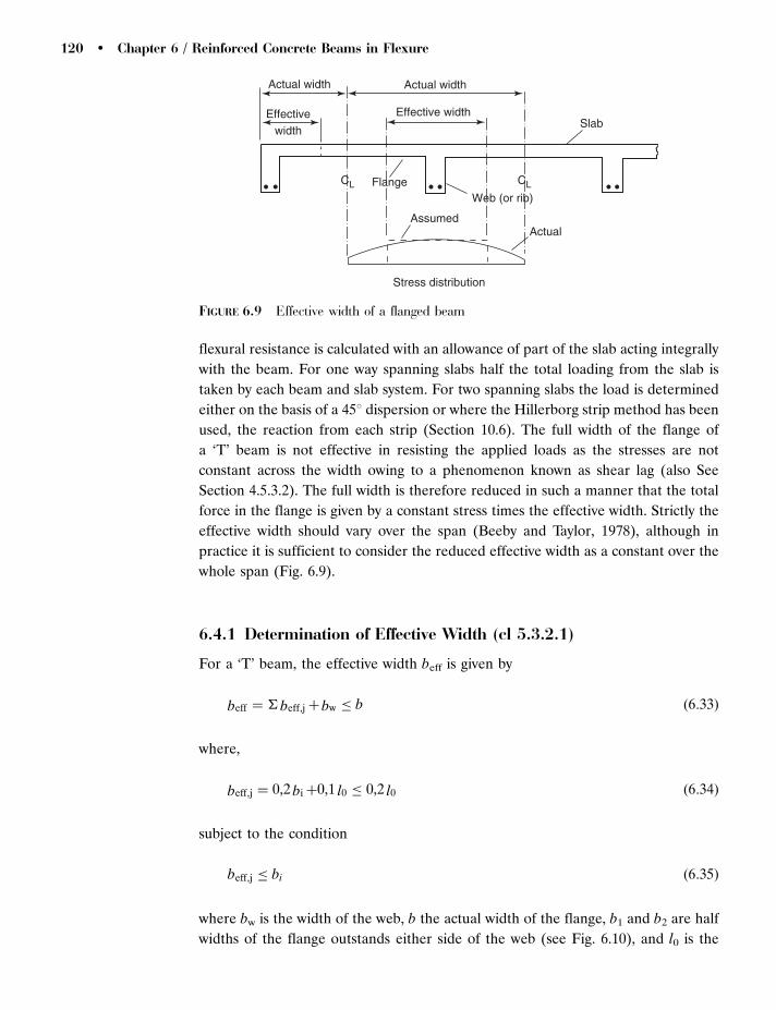
flexural resistance is calculated with an allowance of part of the slab acting integrally
with the beam. For one way spanning slabs half the total loading from the slab is
taken by each beam and slab system. For two spanning slabs the load is determined
either on the basis of a 458 dispersion or where the Hillerborg strip method has been
used, the reaction from each strip (Section 10.6). The full width of the flange of
a ‘T’ beam is not effective in resisting the applied loads as the stresses are not
constant across the width owing to a phenomenon known as shear lag (also See
Section 4.5.3.2). The full width is therefore reduced in such a manner that the total
force in the flange is given by a constant stress times the effective width. Strictly the
effective width should vary over the span (Beeby and Taylor, 1978), although in
practice it is sufficient to consider the reduced effective width as a constant over the
whole span (Fig. 6.9).
6.4.1 Determination of Effective Width (cl 5.3.2.1)
For a ‘T’ beam, the effective width beff is given by
beff ¼ � beff,j þ bw � b ð6:33Þ
where,
beff,j ¼ 0,2 bi þ0,1 l0 � 0,2 l0 ð6:34Þ
subject to the condition
beff,j � bi ð6:35Þ
where bw is the width of the web, b the actual width of the flange, b1 and b2 are half
widths of the flange outstands either side of the web (see Fig. 6.10), and l0 is the
Actual width Actual width
Effective widthSlab
Actual
Stress distribution
Assumed
Web (or rib)FlangeCL CL
Effectivewidth
FIGURE 6.9 Effective width of a flanged beam
120 � Chapter 6 / Reinforced Concrete Beams in Flexure
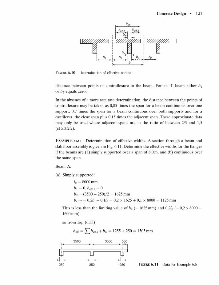
distance between points of contraflexure in the beam. For an ‘L’ beam either b1
or b2 equals zero.
In the absence of a more accurate determination, the distance between the points of
contraflexure may be taken as 0,85 times the span for a beam continuous over one
support, 0,7 times the span for a beam continuous over both supports and for a
cantilever, the clear span plus 0,15 times the adjacent span. These approximate data
may only be used where adjacent spans are in the ratio of between 2/3 and 1,5
(cl 5.3.2.2).
EXAMPLE 6.6 Determination of effective widths. A section through a beam and
slab floor assembly is given in Fig. 6.11. Determine the effective widths for the flanges
if the beams are (a) simply supported over a span of 8,0 m, and (b) continuous over
the same span.
Beam A:
(a) Simply supported:
l0 ¼ 8000 mm
b1 ¼ 0, beff,1 ¼ 0
b2 ¼ ð3500 � 250Þ=2 ¼ 1625 mm
beff,2 ¼ 0,2bi þ 0,1l0 ¼ 0,2 � 1625 þ 0,1 � 8000 ¼ 1125 mm
This is less than the limiting value of b2 (¼ 1625 mm) and 0,2l0 (¼ 0,2� 8000¼
1600 mm)
so from Eq. (6.33)
beff ¼X
beff,j þ bw ¼ 1255 þ 250 ¼ 1505 mm
b2b2b1b1
bw
bw
beff
beff,1 beff,2
b
FIGURE 6.10 Determination of effective widths
250 250
3500 3500 500
250 FIGURE 6.11 Data for Example 6.6
Concrete Design � 121

(b) Continuous:
l0 ¼ 0,7 � 8000 ¼ 5600 mm. The values of b1, b2 and beff,1 are same as above.
beff,2 ¼ 0,2bi þ 0,1l0 ¼ 0,2 � 1625 þ 0,1 � 5600 ¼ 885 mm
This is less than the limiting value of b2 (¼ 1625 mm) and 0,2l0 (¼ 0,2� 5600¼
1120 mm)
so from Eq. (6.33)
beff ¼X
beff,j þ bw ¼ 885 þ 250 ¼ 1135 mm
Beam B:
(a) Simply supported:
As the beam is symmetric about its centre line, b1¼ b2, and beff,1¼ beff,2
b ¼ 3500 mm
b1 ¼ b2 ¼ ð3500 � 250Þ=2 ¼ 1625 mm
beff,1 ¼ 0,2b1 þ 0,1l0 ¼ 0,2 � 1625 þ 0,1 � 8000 ¼ 1125 mm
This is less than the limits of b1 or 0,2l0.
beff ¼ beff,1 þ beff,2 þ bw ¼ 2 � 1125 þ 250 ¼ 2500 mm:
This is less than the actual width b.
(b) Continuous:
As the beam is symmetric about its centre line, b1¼ b2, and beff,1¼ beff,2
b ¼ 3500 mm
b1 ¼ b2 ¼ ð3500 � 250Þ=2 ¼ 1625 mm
beff,1 ¼ 0,2b1 þ 0,1l0 ¼ 0,2 � 1625 þ 0,1 � 5600 ¼ 885 mm
This is less than the limits of b1 or 0,2l0.
beff ¼ beff,1 þ beff,2 þ bw ¼ 2 � 885 þ 250 ¼ 2020 mm:
This is less than the actual width b.
Beam C:
b1 ¼ 1625 mm ðas in the previous calculationsÞ
b2 ¼ 500 � 250=2 ¼ 375 mm
(a) Simply supported:
beff,1 ¼ 0,2 � 1625 þ 0,1 � 8000 ¼ 1125 mm
122 � Chapter 6 / Reinforced Concrete Beams in Flexure
This is less than the limiting values
beff,2 ¼ 0,2 � 375 þ 0,1 � 8000 ¼ 875 mm
Limiting values are b2 (¼ 375 mm) or 0,2� l0 (¼ 1600 mm)
Thus beff,2¼ 375 mm
From Eq. (6.33)
beff ¼ beff,1 þ beff,2 þ bw ¼ 1125 þ 375 þ 250 ¼ 1750 mm
(b) Continuous:
beff,1 ¼ 0,2 � 1625 þ 0,1 � 5600 ¼ 885 mm
This is less than the limiting values.
beff,2 ¼ 0,2 � 375 þ 0,1 � 5600 ¼ 635 mm
Limiting values are b2 (¼ 375 mm) or 0,2� l0 (¼ 1120 mm)
Thus beff,2 ¼ 375 mm
From Eq. (6.33)
beff ¼ beff,1 þ beff,2 þ bw ¼ 885 þ 375 þ 250 ¼ 1510 mm
6.4.2 Design of a Flanged Beam
Under hogging moments the flange is in tension, and is thus cracked. The beam is
then designed as a rectangular beam (with the tension reinforcement in the top of
the beam, spaced to allow a vibrating poker to compact the concrete adequately,
i.e. a clear space of at least 75 mm should be left between the bars).
Under sagging moments two cases must be considered (Fig. 6.12):
(a) where the neutral axis is in the web, and
(b) where the neutral axis is in the flange.
6.4.2.1 Sagging Moment: Neutral Axis in the Flange
For this case the design follows the calculations for rectangular beams with the width
of the beam taken as the effective width of the flange.
6.4.2.2 Sagging Moment: Neutral Axis in the Web
It is sufficiently accurate to design the tension reinforcement on the basis that the
entire flange is in compression with the centre of compression at the mid-height of
the flange (with any concrete in compression in the web being ignored). Thus As may
Concrete Design � 123

be determined from
MRd ¼AS fyk
1,15d�
tf2
� �ð6:36Þ
where tf is the thickness of the flange. However the moment applied cannot exceed
the value MSd,max based on the capacity of the concrete flange,
MSd, max ¼ 0,85fck
�cbeff tf d�
tf2
� �ð6:37Þ
EXAMPLE 6.7 Design of a ‘T’ beam. A ‘T’ beam has an effective flange width of
1370mm, a flange thickness of 150 mm, a web width of 250 mm and an overall depth
of 500 mm. The concrete Grade is C25 and the steel 500 MPa. The axis distance from
the reinforcement to any face is 50 mm. Design suitable reinforcement for the
following moments (there is no redistribution):
(i) 400 kNm (sagging), and
(ii) 300 kNm (hogging).
(a) effective depth d¼ 500� 50¼ 450 mm
Check the moment capacity of the beam assuming the neutral axis is in the web
with the complete flange available to resist compression using Eq. (6.37),
MSd ¼ ð0,85 � 25 � 1370 � 150=1,5Þ ð450 � 150=2Þ10�6 ¼ 1091 kNm:
d
beff
tf
x
tf / 2
Fc
Neutralaxis
Neutralaxis
Concrete betweentable of flange &neutral axis isignored
(a) Neutral axis in web
(b) Neutral axis in flange
FIGURE 6.12 ‘T’ Beam design
124 � Chapter 6 / Reinforced Concrete Beams in Flexure
Neutral axis is therefore in the flange as this value exceeds the applied moment.
So use Eq. (6.22) (with b replaced by beff):
Msd=beffd2fck ¼ 400 � 106=1370 � 4502 � 25 ¼ 0,0577
As fyk=beffdfck ¼ 0,652 �pð0,425 � 1,5 � 0,0577Þ ¼ 0,070
As ¼ 0,070 � 1370 � 450 � 25=500 ¼ 2158 mm2
Fix 3D32 (2413 mm2)
Check x/d:
x=d ¼ 1,918As fyk=beffdfck ¼ 1,918 � 0,070 ¼ 0,1345 0,45
(b) d¼ 450 mm (as above): b¼ bw¼ 250 mm
MSd.max/bd2fck for a singly reinforced beam is 0,168 (Table 6.2).
MRd:max ¼ 0,168 � 250 � 4502 � 25 � 10�6 ¼ 213 kNm5MSd
Beam requires compression reinforcement.
As, lim ¼ 0,234 � 450 � 250 � 25=500 ¼ 1294 mm2
MSd=bd2fck ¼ 300 � 106=250 � 4502 � 25 ¼ 0,237
d0=d ¼ 50=450 ¼ 0,111:
xlim=d ¼ 0,45:
Check d0/d Eq. (6.31):
d0=d ¼ ðxlim=d Þð1 � fyk=805Þ ¼ 0,45ð1 � 500=805Þ ¼ 0,170:
Actual d0/d is less than the limiting value, so compression steel has yielded.
MRd,add=bd2fck ¼ 0,237 � 0,168 ¼ 0,069
Calculate A0s from Eq. (6.29)
A0s fyk=bdfck ¼ 0,069=ð1 � 0,111Þ ¼ 0,0776
Asl ¼ 0,0776 � 250 � 450 � 25=500 ¼ 437 mm2
Fix 2D20 (628 mm2)
As ¼ As, lim þ A0s ¼ 1249 þ 437 ¼ 1686 mm2
Fix 2D40 (2513 mm2) (this arrangement gives a clear enough space between the
bars to allow full compaction of the concrete. An alternative would be to either
bundle bars or to place steel in two layers with a subsequent recalculation of
moment capacity).
Concrete Design � 125

EXAMPLE 6.8 Design of a T beam. A beam with a flange width of 1500 mm, flange
thickness 150 mm, effective depth 800 mm and web width 350 mm carries a moment
of 2000 kNm. Concrete Grade C25 and steel strength 500 MPa. Design suitable
reinforcement.
Initially calculate the moment capacity assuming the neutral axis is at the top of
the web (or the underside of the flange).
x/d¼ 150/800¼ 0,1875
Using Eq. (6.19)
As fyk
b d fck¼ 1,918
x
d¼ 1,918 � 0,1875 ¼ 0,36 ð6:38Þ
Using Eq. (6.18)
MRd
b d2fck¼
As fyk
b d fck1 � 0,4
x
d
� �¼ 0,36ð1 � 0,4 � 0,1875Þ ¼ 0,333 ð6:39Þ
or, MRd ¼ 0,333 � 1500 � 8002 � 25 � 10�6 ¼ 7992 kNm:
This is greater than the applied moment of 2000 kNm, thus the neutral axis is in the
flange.
As a check, the moment capacity M assuming the neutral axis is the web with
the concrete fully stressed is given by
M ¼ bf tf �ccfck
�c
� �d�
tf2
� �
¼ 1500 � 150 � 0,85 �25
1,5
� �800 �
150
2
� �� 10�6
¼ 2311 kNm ð6:40Þ
MSd is less than either of these limiting values, thus beam is singly reinforced with
the neutral axis in the flange. MSd/bf d2fck¼ 2000� 106/1500� 8002
� 25¼ 0,0833
Use Eq. (6.22) to determine Asfyk/bw dfck:
As fck
b d fck¼ 0,652 �
ffiffiffiffiffiffiffiffiffiffiffiffiffiffiffiffiffiffiffiffiffiffiffiffiffiffiffiffiffiffiffiffiffiffiffiffiffi0,425 � 1,5
MSd
b d2fck
s
¼ 0,652 �ffiffiffiffiffiffiffiffiffiffiffiffiffiffiffiffiffiffiffiffiffiffiffiffiffiffiffiffiffiffiffiffiffiffiffiffiffiffiffiffiffiffi0,425 � 1,5 � 0,0833
p¼ 0,104 ð6:41Þ
As ¼ 0,104 � 1500 � 800 � 25=500 ¼ 6240 mm2
Fix 6D40 [7540 mm2] in TWO layers. This will reduce the effective depth, but the
reinforcement is overprovided.
Check x/d from Eq. (6.19):
x
d¼
1
1,918
As fyk
b d fck¼
0,104
1,918¼ 0,054 ð6:42Þ
126 � Chapter 6 / Reinforced Concrete Beams in Flexure

x¼ 0,054d¼ 0,054� 800�¼ 43,2 mm (this is within the flange).
Fix 8D40 (10,500 mm2) in TWO layers.
6.5 HIGH STRENGTH CONCRETE
Although, high strength concrete is not commonly used in cases where flexure is
dominant as it is the steel strength which tends to control behaviour, it will allow
slightly less shear reinforcement and give improved deflection behaviour as the
empirical rules are dependant on the concrete strength.
The design procedure is essentially similar to that for more normal strength
concretes except the parameters needed with the flexural design Eq. (6.12) to (6.15)
need evaluating for each concrete strength.
Two examples (based on Examples 6.1 and 6.4) will be carried out to demonstrate
the differences.
EXAMPLE 6.9 Design of a singly reinforced section. A singly reinforced beam
has a width of 300 mm and an effective depth of 600 mm. The concrete is Grade C70
and the steel is Grade 500. Determine
(a) the maximum design moment of resistance of the section and determine the
reinforcement necessary. If the maximum aggregate size is 20 mm and the cover
to the main reinforcement is 40 mm, and,
(b) the area of reinforcement required to resist a moment of 350 kNm.
Limiting neutral axis depth is determined from Eq. (6.7). However it is first
necessary to determine "cu2:
"cu2 ¼ 2,6 þ 3590 � fck
100
� �4 !
� 10�3
¼ 2,6 þ 3590 � 70
100
� �4 !
� 10�3
¼ 2620 � 10�6 ð6:43Þ
Equation (6.7) may be rewritten as
x
d¼
�� 0,54
1,25 0,6 þ0,0014
"cu2
� �
¼1 � 0,54
1,25 0,6 þ0,0014
2620 � 10�6
� � ¼ 0,324 ð6:44Þ
Concrete Design � 127

(as there is no redistribution, �¼ 1,0) Determine � from (6.17)
� ¼ 1,0 �fck � 50
200¼ 1 �
70 � 50
200¼ 0,9 ð6:45Þ
and � from (6.16)
� ¼ 0,8 �fck � 50
400¼ 0,8 �
70 � 50
400¼ 0,75 ð6:46Þ
Use Eq. (6.11) to determine the relationship between As fyk/bdfck and x/d,
As fyk
b d fck¼�s�� �cc
�c
x
d
¼1,15 � 0,9 � 0,75 � 0,85
1,5
x
d¼ 0,44
x
dð6:47Þ
With the limiting value of x/d,
As fyk=bdfck ¼ 0,44 � 0,324 ¼ 0,143
Use Eq. (6.13) to determine M/bd2fck:
MSd
b d2fck¼
As fyk
b d fck1 �
�
2
x
d
� �
¼ 0,143 1 �0,75
2� 0,324
� �¼ 0,126 ð6:48Þ
MSd ¼ 0,126 � 300 � 6002 � 70 � 10�6 ¼ 952 kNm:
As fyk=b d fck ¼ 0,143, so
As ¼ 0,143 � 300 � 600 � 70=500 ¼ 3604 mm2
Fix 2D32 and 2D40 (As¼ 4122 mm2)
Minimum spacing between bars is greater of bar diameter or 20 mm.
Minimum width required ¼ 2 � 32 þ 3 � 40 þ 2 � 40 þ 2 � 40
¼ 284 mm5 300 mm
Therefore satisfactory overall depth is 600þ 40/2þ 40¼ 660 mm.
(b) Steel area for moment of 350 kNm.
MSd=bd2fck ¼ 350 � 106=ð300 � 6002 � 70Þ ¼ 0,0463:
Use Eq. (6.15) to determine As fyk/bdfck, however the coefficients in this equation
need to be calculated first
�s� �cc�c
¼1,15 � 0,9 � 0,85
1,5¼ 0,587 ð6:49Þ
128 � Chapter 6 / Reinforced Concrete Beams in Flexure
2�2s ��cc
�c¼
2 � 1,152 � 0,9 � 0,85
1,5¼ 1,35 ð6:50Þ
So Eq. (6.15) becomes
As fyk
b d fck¼ 0,587 �
ffiffiffiffiffiffiffiffiffiffiffiffiffiffiffiffiffiffiffiffiffiffiffiffiffiffiffiffiffiffiffiffiffiffiffiffiffiffiffiffi0,5872 � 1,35
M
bd2fck
s
¼ 0,587 �ffiffiffiffiffiffiffiffiffiffiffiffiffiffiffiffiffiffiffiffiffiffiffiffiffiffiffiffiffiffiffiffiffiffiffiffiffiffiffiffiffiffiffiffiffiffiffi0,5872 � 1,35 � 0,0463
p¼ 0,0555 ð6:51Þ
As ¼ 0,0555 � 600 � 300 � 70=500 ¼ 1399 mm2:
Fix 3D25 in a single layer (1473 mm2).
Check x/d from Eq. (6.11):
x=d ¼ ð1=0,44ÞAs fyk=bdfck ¼ 2,273 � 0,0555 ¼ 0,1265 0,324 (determined in (a)).
EXAMPLE 6.10 Design of a doubly reinforced section. A doubly reinforced
beam constructed from Grade C70 concrete has a width of 250 mm and an effective
depth of 450 mm. The reinforcement has a characteristic strength of 500 MPa, and
the axis depth of the compression reinforcement, if required, is 50 mm. If the
moment applied to the section is 400 kNm, determine the reinforcement
requirements for (a) no redistribution and (b) a reduction of 20 per cent due to
redistribution.
The necessary design, Eqs (6.44), (6.47) and (6.51) have already been derived in
Example 6.9 and will not be repeated.
(a) Maximum x/d¼ 0,324 (from Example 6.9)
Maximum moment without compression steel:
MRd,max=bd2fck ¼ 0,126 as before
MRd,max ¼ 0,126 � 250 � 4502 � 70 � 10�6 ¼ 447 kNm
As MSd is less than the maximum value, the beam is singly reinforced.
MSd=bd2fck ¼ 400 � 106=250 � 4502 � 70 ¼ 0,113
Using Eq. (6.51)
As fyk=bdfck ¼ 0,587 �pð0,5872 � 1,35 � 0,113Þ ¼ 0,149
As ¼ 0,149 � 250 � 450 � 70=500 ¼ 2347 mm2
Fix 3D32 (2412 mm2)
Concrete Design � 129
(b) 20 per cent reduction due to redistribution (�¼ 0,8)
Use Eq. (6.44) to determine limiting x/d value
x
d¼
�� 0,54
1,25 0,6 þ0,0014
"cu2
� �
¼0,8 � 0,54
1,25 0,6 þ0,0014
2620 � 10�6
� � ¼ 0,184 ð6:52Þ
Limiting value of As fyk/bdfck from Eq. (6.47)
As fyk
b d fck
� �lim
¼ 0,44 � 0,184 ¼ 0,0810 ð6:53Þ
As,lim ¼ 0,0810 � 500 � 250 � 70=500 ¼ 1418 mm2
Limiting value of M/bd2fck is given by Eq. (6.13)
MSd
b d2fck¼
As fyk
b d fck1 �
�
2
x
d
� �
¼ 0,0810 1 �0,75
2� 0,184
� �¼ 0,0754 ð6:54Þ
MSd=bd2fck ¼ 400 � 106=250 � 4502 � 70 ¼ 0,113
This is greater than the limiting value, therefore compression steel is
required, so,
MRd,add=bd2fck ¼ MSd=bd
2fck �MRd, lim=bd2fck
¼ 0,113 � 0,0754 ¼ 0,0376
Check yield status of the compression reinforcement with x/d¼ 0,185
Critical value of d0/d is given by a similar equation to Eq. (6.31) but with the
constant replaced by
1,15 � 200 � 103"cu2 ¼ 1,15 � 200 � 103 � 2660 � 10�6 ¼ 612 ð d0=d Þcrit
¼ ðxlim=dÞ ð1 � fyk=612Þ
¼ 0,184 � ð1 � 500=612Þ ¼ 0,034
Actual d0/d¼ 50/450¼ 0,111.
The compression steel has not therefore yielded, and its stress level fs is given
by Eq. (6.32) with the constant replaced by 612/1,15¼ 532,
fs ¼ 532ð1 � ðd0=dÞ ðd=xlimÞÞ ¼ 532ð1 � 0,111=0,184Þ ¼ 211 MPa
130 � Chapter 6 / Reinforced Concrete Beams in Flexure
From Eq. (6.29) with the steel yield stress replaced by its elastic stress,
A0s fs=bdfck ¼ ðMRd,add=bd
2fckÞ=ð1 � d0=dÞ
¼ 0,0376=ð1 � 0,111Þ ¼ 0,0334
A0s ¼ 0,0334 � 250 � 450 � 70=211 ¼ 1247 mm2:
Fix 2D32 (1608 mm2)
Two bars are preferred to three in order to give the maximum space possible
between the top steel to allow a 75 mm diameter poker vibrator to be able to
reach the complete cross section. Additional tension steel, As,add.
Since the compression steel has not yielded then this must be given by an
equivalent area of yielded steel, so
As,add ¼ A0s fs =ð fyk=1,15Þ ¼ 1247 � 211=ð500=1,15Þ ¼ 606 mm2
As,total ¼ As,lim þ As,add ¼ 1418 þ 606 ¼ 2024 mm2
Fix 4D32 (3217 mm2).
6.6 DESIGN NOTES
6.6.1 Sizing of Sections
The size of sections are generally constrained by the situation in which they are being
used, e.g. the width of a beam must be sufficient to provide the requisite bearing
lengths for precast floor units, or sufficient to support both leaves of a cavity wall.
The construction depth should be the least possible, except that it is cheaper and
easier to construct formwork for a beam layout when all the soffits are at the same
level and the beams are no narrower than the columns into which they frame.
Where there are no limitations the most effective section is one in which the width is
around half the depth. The depth for a preliminary design can be taken between 1/10
to 1/15 of the span, with the higher figure being used for longer spans.
6.6.2. Procedure for Design of Beams
(1) Check the allowable x/d ratio (with consideration being taken of redistribution,
if appropriate).
(2) Determine the maximum moment MRd,lim capacity at the limiting x/d ratio.
(3) Determine whether the applied moment MSd is greater or less than MRd,lim.
(4) If less, the beam is singly reinforced and As determined from Eq. (6.22) for
�cc¼ 0,85 and Eq. (6.27) for �cc¼ 1,0.
(5) If greater, beam needs compression reinforcement with A0s determined from
Eq. (6.29). Note, compression steel needs checking for yield.
(6) In all cases minimum and maximum percentages of steel should be checked.
(The minimum steel requirement will often govern for slab design).
Concrete Design � 131

(7) Design shear reinforcement.
(8) Check bar spacing and span/effective depth ratio for deflection and cracking.
Note reinforcement in the top face of a beam should have clear spacing of at
least 75 mm to allow the insertion of a poker vibrator.
6.7 EFFECTIVE SPANS (cl 5.3.2.2)The effective span leff used to determine the internal forces in a member should
be taken as
leff ¼ ln þ a1 þ a2 ð6:55Þ
where ln is the clear distance between the supports and a1 and a2 are the end
distances at either end of the element and are determined from Fig. 6.13. For beams
supported on bearings the effective span is the distance between the centre lines of
the bearings. For columns the effective heights are those between beam centre lines.
REFERENCES AND FURTHER READING
Baldwin, R. and North, M.A. (1973) A stress–strain relationship for concrete at high temperatures.
Magazine of Concrete Research, 24, 99–101.
Beeby, A.W. and Taylor, H.P.J. (1978) The use of simplified methods in CP110- is rigour necessary?
Structural Engineer, 56A(8), 209–215.
Moss, R. and Webster, R. (2004) EC2 and BS8110 compared. The Structural Engineer, 82(6), 33–38.
(a) Wall support (also applies to continuous members)
Leff
Ln
ai
t
Lesser of
(b) Restrained support (or cantilever)
h2
t2
or
h
Leff
Ln
ai
ai Lesser of h2
h
t
t2
or
FIGURE 6.13 Determination ofeffective spans
132 � Chapter 6 / Reinforced Concrete Beams in Flexure

C h a p t e r 7 / Shear and Torsion
7.1 SHEAR RESISTANCE OF REINFORCED CONCRETE
7.1.1 Introduction (cl 6.2, EN)
The dimensions of the cross section of a reinforced concrete beam and the area of
longitudinal steel are usually determined from calculations which consider resistance
to the bending at the ultimate limit state. In situations of minor importance, e.g. a
lintel, these dimensions and reinforcement will be adequate to resist small transverse
shear forces. In other cases at least minimum shear reinforcement is required, and
where shear forces in beams are large shear reinforcement must be added to resist
all of the shear force.
7.1.2 Types of Shear Failure
The mechanism of shear failure in reinforced concrete is complicated and despite
extensive experimental and theoretical research work semi-empirical solutions are
currently still in use. The appearance of a beam failing in shear is shown in Fig. 7.1,
and may be described as cracked concrete interacting with, and held together by the
reinforcement. Prior to failure, vertical cracks are produced by the bending moment
but later these are linked to diagonal cracks produced by the shear forces. Broadly
there are five types of failure for reinforced concrete beams as shown in Fig. 7.1. The
diagrams show the left hand support for a simply supported beam carrying a central
point load. The first four types of failure are related to the shear span ratio (a/d). As
the shear span ratio increases shear resistance decreases, but for values of a/d4 3
the decrease is relatively small. The longitudinal steel does not generally reach yield.
Type I (a/d4 6) The bending moment is large in comparison to the shear force and
the mode of failure is similar to that in pure bending, i.e. rotation about the
compression zone. The initial vertical bending cracks become inclined due to the
action of the shear stresses and failure occurs in the compression zone (Fig. 7.1(a)).
The stresses in the tensile steel are close to yield and only minimum shear
reinforcement is required in design situations.

Type II (64 a/d4 2) The initial bending cracks become inclined early in the loading
sequence and failure is associated more with vertical shear deformation and less with
vertical shear deformation and less with rotation about the compression zone. At
collapse, horizontal cracks form running along the line of the tensile reinforcement
(Fig. 7.1(b)) which reduce the shear resistance of the section by destroying the dowel
force, which reduces the bond stresses between the steel and concrete. Finally the
compression zone fails when subject to shear and compression.
Type III (a/d5 2) Bending cracks are small and do not develop but shear cracks,
connecting a load point and the support, suddenly appear and run through to the
compression zone producing collapse (Fig. 7.1(c)).
Type IV (av/d¼ 0) Punching shear failure occurs when the plane of failure is forced
to run parallel to the shear forces as shown in Fig. 7.1(d). This can occur when the
opposing shear forces are close together or, if vertical shear links have been added,
when a failure plane forms which does not intercept the shear links. When this type
of failure occurs the shear resistance of the section is at a maximum. The addition of
shear reinforcement in the form of horizontal or inclined links increases the shear
resistance.
Type V The addition of shear reinforcement increases the shear resistance provided
that the shear reinforcement intercepts the shear cracks. Numerous diagonal cracks
develop as shown in Fig. 7.1(e) and at failure the shear reinforcement reaches yield,
provided that the shear reinforcement is anchored and not excessive.
Shear crackCompressionzone crushes
Dowel force crackleading to bond failure
Crack extendsinto compressionzone
Bending crack
Shear crack suddenlyappears rapidlyfollowed by failurein the compression zone
(a) Type I a /d>6
(c) Type III a /d < 2 (d) Type IV a /d = 0 Punching shear
(b) Type II 6>a /d>2
(e) Type V Shear reinforcement
Vertical links
Bent-up bars
Multiple cracks
V V
d d
d
a a
a
V VV
FIGURE 7.1 Types of shear failure in reinforced concrete beams
134 � Chapter 7 / Shear and Torsion

7.1.3 Components of Shear Resistance
The shear resistance of a section may be represented by component strength parts as
shown in Fig. 7.2. The approximate percentage of the total shear load resisted by
each component, obtained experimentally (Taylor, 1974) for a singly reinforced
concrete beam without shear reinforcement, is indicated.
The shear resistance of a beam can be expressed as the sum of the resistance of the
parts, but the exact interaction of these shear components is not fully understood,
and theories which are reasonably accurate are often too complicated for use in
practical situations. Experiments (ASCE-ACI, 1973) show that the shear resistance
increases with an increase in, area of the section, area of the tensile steel, direct
compressive stress and strength of the concrete. These variables are included in
Eq. (7.1). Except for small percentage of steel, the steel does not yield and
therefore the yield strength of the longitudinal steel is not a variable.
7.2 MEMBERS NOT REQUIRING SHEAR REINFORCEMENT (cl 6.2.2, EN)
Shear reinforcement is not required in slabs of less than 200 mm nor for members of
minor importance, e.g. a lintel. The reasons are that loading on a lintel is low, while
for a slab the depth is often insufficient to accommodate shear reinforcement. The
following equation is largely based on empirical evidence.
Design shear resistance (Eq. 6.2a, EN)
VRd,c ¼ ½CRd,ckð1001 fckÞ1=3
þ k1cp�bwd ð7:1Þ
where
VRd,c4ðvmin þ k1cpÞbwd and vmin ¼ 0,035k1,51 f 0,5
ck
CRd,c ¼ 0,18=�c
bw is the minimum width of the section in the tensile area
Compression zone (20−40%)
Aggregate interlock (35−50%)
Tensile force steel
Vertical linksDowelforce
(15−25%)
V
FIGURE 7.2 Components of shear resistance for a singly reinforced beam
Concrete Design � 135

k¼ 1þ (200/d)0,5 where d is in mm
l ¼ Asl=ðbwdÞ � 0,02
Asl¼ the area of tension reinforcement extending not less than dþ lbd beyond the
section considered
cp ¼ NEd=Ac 5 0,2fcd MPa
NEd¼ axial force in the section due to loading or prestressing (compression positive)
k1 ¼ 0,15
Where shear cracks are restrained by the loading point and support, and where
0,5d� av� 2d, the shear force may be reduced by �¼ av/2d. For av� 0,5d, av¼ 0,5d
(cl 6.2.2(6), EN). The longitudinal reinforcement must be anchored securely at the
support.
The factor k indicates that shear resistance decreases with increase in depth, which is
justified by experiments (Chana, 1981 and Shioya et al., 1989). The reason is thought
to be due to larger crack widths in deep beams (ASCE-ACI, 1998). The resistance of
the longitudinal steel is related to the steel ratio and does not include the yield
strength.
The maximum shear force, calculated without the reduction factor �, that a section
can resist (Eq. 6.5, EN) is related to the crushing strength of the concrete
VRd � 0,5bwdn fcd ð7:2Þ
where the strength reduction factor for concrete cracked in shear (cl 6.6, EN)
n ¼ 0:6 ð1 � fck=250Þ
EXAMPLE 7.1 Shear resistance of a singly reinforced concrete lintel beam. A
simple supported lintel beam spans 2 m and carries a total uniformly distributed
design load of 15,8 kN. The beam section is 230 mm square (d¼ 200) with 2T10 bars
in tension which are sufficient to resist bending at midspan. Determine the shear
resistance as a singly reinforced beam assuming C20/25 Grade concrete.
Reduced design shear force at a distance d from the support (cl 6.2.1(8), EN)
VEd ¼ ðL=2 � dÞ=ðL=2Þ �W=2 ¼ ð2000=2 � 200Þ=ð2000=2Þ � 15,8=2 ¼ 6,3 kN
Shear force resistance of a singly reinforced section (Eq. 6.2a, EN)
VRd,c ¼ ½CRd,ckð100l fckÞ1=3
þ 0,15cp�bwd
¼ ½0,18=1,5 � 2ð100 � 0,00343 � 20Þ1=3 þ 0� � 230 � 200=1E3
¼ 21,04VEdð6,3Þ kN, therefore satisfactory:
136 � Chapter 7 / Shear and Torsion
Minimum shear resistance
vmin ¼ 0,035 k1,5f 0,5ck ¼ 0,035 � 21,5 � 200,5 ¼ 0,443
vmin ¼ ðvmin þ k1cpÞbwd
¼ ð0,443 þ 0Þ � 230 � 200=1E3 ¼ 20,45VRd,cð21,0Þ kN, satisfactory:
Longitudinal tensile reinforcement ratio (cl 6.2.2(1), EN)
l ¼ As=ðbwdÞ ¼ 2 � 79=ð230 � 200Þ ¼ 0,0034350,02, acceptable:
Minimum area of the longitudinal steel (cl 9.2.1.1, EN) which includes
fctm ¼ 2,2 MPa from Table 3.1, EN (Annex A2)
l,min ¼ 0,26fctm=fyk ¼ 0,26 � 2,2=500 ¼ 0,001145lð0,00343Þ, satisfactory:
Depth factor
k ¼ 1 þ ð200=dÞ0,5¼ 1 þ ð200=200Þ0,5
¼ 2
This is a member of minor importance and shear reinforcement is not required
(cl 6.2.1(4), EN).
Maximum shear resistance (Eq. 6.5, EN), generally not critical for a lintel beam
VRd, max ¼ 0,5bwdnfcd ¼ 0,5 � 230 � 200 � 0,552 � ð20=1,5Þ=1E3
¼ 169,34VEd, maxð7,9Þ kN, therefore satisfactory:
where the strength reduction factor (Eq. 6.6 EN)
n ¼ 0,6ð1 � fck=250Þ ¼ 0,6ð1 � 20=250Þ ¼ 0,552
7.3 MEMBERS REQUIRING SHEAR REINFORCEMENT (cl 6.2.3, EN)At the ultimate limit state, where the design shear force is greater than the resistance
of a singly reinforced beam, then shear reinforcement is required to resist all of the
applied shear force. The most common type of shear reinforcement is in the form of
vertical stirrups, or links, spaced at intervals along the length of a member. The links
should be well anchored (cl 8.5, EN). The shape of the link, shown in Fig. 7.3(b), is
preferred because it is closed, but the other shapes shown in Fig. 7.3(c) and (d) are
also used where there are practical difficulties in fixing the reinforcement. See
also Fig. 9.5, EN. Vertical links strengthen the beam web and resist dowel failure
(Fig. 7.1(b)).
The European Code method for the shear resistance of a beam with vertical links is
based on the traditional truss analogy (Ritter, 1899). The truss consists of a tie BC at
Concrete Design � 137

an angle � which represents the links acting over a length AC, a compression strut
AB representing a concrete compression at an angle �, together with longitudinal
tension and compression reinforcement (Fig. 7.4). The truss analogy applies to
vertical and inclined links or bars.
Resolving forces vertically at section 1-1 (Fig. 7.4) to check for strength of a link
(Eq. 6.13, EN).
VRd,s ¼ Fsw sin � ¼ AswfywdðAC=sÞ sin � ¼ Asw=sfywdzðcot � þ cot�Þ sin � ð7:3Þ
To check for the crushing of the equivalent concrete strut resolve forces vertically at
section 2-2 (Eq. 6.14, EN).
VRd, max ¼ Fcn sin � ¼ fckbwðAC sin �Þ sin � ¼ �c fcdbwzðcot � þ cot�Þ sin2 �
¼ �c fcdbwzðcot � þ cot�Þ=ð1 þ cot2 �Þ ð7:4Þ
The factor �c is introduced for design purposes to allow for the effect of shear,
cracking and prestressing on concrete. The strength of the steel tie BC should be less
than the strength of the concrete strut AB.
Compression reinforcement
V
s
d0.9
1070 mm 550 mm
Tensionreinforcement
(a)
(b) (c) (d)
f</
FIGURE 7.3 Types of vertical links
Conc.strut
Tension reinf.
Inclinedsteel
Compression reinf.
FcnFsw
q aA
B
C
12
12
V
V (cotq − cota)
V
Z =
0,9
d
FIGURE 7.4 Truss analogy
138 � Chapter 7 / Shear and Torsion
The additional tensile force in the tension steel due to shear is obtained from the
equilibrium of horizontal forces (Eq. 6.18, EN)
2�Ftd ¼ Fcn cos � � Fsw cos� ¼ VEd= tan � � VEd= tan �
�Ftd ¼ 0,5VEdðcot � � cot �Þ ð7:5Þ
Total force in the tension steel
MEd=zþ�Ftd � MEd, max=z ð7:6Þ
These last two equations are used to determine the longitudinal compression steel
and to check that there is sufficient tension steel at sections where the bending
moment and shear force are large.
7.3.1 Minimum, or Nominal, Vertical Links (cl 9.2.2 EN)
In most building construction work the smallest diameter link is 6 mm and
the largest diameter is generally 12 mm. 12 mm diameter links are not often used
because of the difficulties involved in bending and because of the displace-
ment of the longitudinal bars at the corners of links when large corner radii are
used.
If too little shear reinforcement is provided it is not effective (Yoon et al., 1996).
It is also required to control cracking and to provide ductility. This is estimated
from the shear ratio (Eq. 9.4, EN)
w ¼ Asw=ðsbw sin �Þ ð7:7Þ
Minimum values of the shear ratio (Eq. 9.5, EN)
w, min ¼ 0,08f 0,5ck =fyk ð7:8Þ
7.3.2 Spacing of Links (cl 9.2.2, EN)
In practice longitudinal spacings of links are generally in intervals to 20 mm. If the
longitudinal spacing of links is greater than approximately 0,75d then the links will
not intercept cracks, nor the distance AC in Fig. 7.4 and consequently will not be
effective in resisting the applied shear force.
Recommendations for minimum longitudinal spacing for links are related to the
requirement for the concrete to flow round the reinforcement during casting.
Hence a space of at least the diameter of the maximum size of aggregate plus 5 mm,
or bar diameter if greater, is required.
Concrete Design � 139
For vertical links the maximum longitudinal spacing (Eq. 9.6, EN)
sl,max ¼ 0,75dð1 þ cot�Þ ð7:9Þ
For bent-up bars to intercept AC (Fig. 7.4) the maximum longitudinal spacing
(cl 9.2.2(7), EN)
sb, max ¼ ð0,9d=1,5Þðcot � þ cot �Þ ¼ 0,6dð1 þ cot �Þ ð7:10Þ
Maximum transverse spacing of legs in a series of shear links (cl 9.2.2(8), EN)
st, max ¼ 0,75d � 600 mm ð7:11Þ
7.3.3 Anchorage of Links (cls 8.5 and 9.2.2, EN)
Generally, it is not possible to anchor a link by bond alone because of the limited
bond length available, and therefore it is necessary to provide longitudinal bars in
the bottom and top of a beam which are enclosed by the link and used as an
anchorage. This arrangement produces a cage of reinforcement which is easier for
the steel fixer to construct, as a separate unit and place in the mould prior to casting
a beam. The longitudinal bars should be at least equal in diameter to the link and
generally are not less than 12 mm, although some designers may use larger sizes.
The shape of link shown in Fig. 7.3(b) is the most effective and common form
used in practice.
7.3.4 Crack Control for Links (cl 7.3, EN)
Cracks are normal in reinforced concrete structures that are stressed, and if they do
not impair the functioning of the structure they are accepted. If calculations are
made acceptable values are 0,25w5 0,4 mm. Cracking is controlled without
calculation by limiting the tensile stress in the steel and by limiting bar spacing
(cl 7.3.3, EN). See Chapter 5 for further information.
EXAMPLE 7.2 Beam with vertical links. A simply supported beam, span 20d,
carries a uniformly distributed design load of 475 kN which includes self weight.
The beam cross section in Fig. 7.5 shows the tension reinforcement required to resist
the bending moment at midspan at the ultimate limit state. Design the cross section
for shear using C30/35 concrete assuming no bar curtailment.
Reduced design shear force at distance d supports (cl 6.2.1(8), EN)
VEd ¼ ð10d� dÞ=ð10dÞ �W=2
¼ ð10 � 0,55 � 0,55Þ=ð10 � 0,55Þ � 475=2 ¼ 213,75 kN
140 � Chapter 7 / Shear and Torsion

Stage (a) Check shear force resistance as singly reinforced (Eq. 6.2a, EN)
VRd,c ¼ ½CRd,ckð100l fckÞ1=3
þ0,15cp�bwd¼ ½0,18=1,5�1,6ð100�0,0167�30Þ1=3 þ0��
350�550=1E3 ¼136,15VEdð213,75Þ kN, add links to resist all of the shear force.
Minimum shear resistance
vmin ¼ 0,035k1,5f 0,5ck ¼ 0,035 � 1,61,5 � 300,5 ¼ 0,388
Vmin ¼ ðvmin þ k1cpÞbwd
¼ ð0,388 þ 0Þ � 350 � 550=1E3
¼ 74,75VRd,cð136,1Þ kN; satisfactory:
Depth factor
k ¼ 1 þ ð200=dÞ0,5¼ 1 þ ð200=550Þ0,5
¼ 1,6
Longitudinal reinforcement ratio (cl 6.2.2(1), EN)
l ¼ As=ðbwdÞ ¼ 3217=ð350 � 550Þ ¼ 0,016750,02
Minimum longitudinal reinforcement ratio (cl 9.2.1.1, EN)
l, min ¼ 0,26fctm=fyk ¼ 0,26 � 2,9=500 ¼ 0,00515lð0,0167Þ, acceptable:
Stage (b) Solution with single vertical links to resist all of the shear force (�¼ 458,�¼ 908) (Eq. 6.8, EN)
Asw=sl ¼ VEd=ðz fywd cot �Þ ¼ ð213,75E3=ð0,9 � 550 � 0,8 � 500 � 1Þ ¼ 1,08 mm
Assuming T8 mm diameter single vertical links, longitudinal spacing
sl ¼ Asw=1,08 ¼ 2 � 50=1,08 ¼ 92,6 mm, use sl ¼ 80 mm:
Maximum shear resistance of the concrete (Eq. 6.9, EN) with n¼ 0,6 for� 60 MPa
VRd, max ¼ �cwbwznfcd=ðcot � þ tan �Þ
¼ 1,0 � 350 � 0,9 � 550 � 0,6 � 30=1,5=ð1 þ 1Þ � 1E-3
¼ 10404VEd, maxð237,5Þ kN; therefore satisfactory:
4T32
T8-80
2T12
d =
550
bw = 350
fck = 30 FIGURE 7.5 Example: beam with verticallinks
Concrete Design � 141

Maximum longitudinal spacing of vertical links (Eq. 9.6, EN)
sl, max ¼ 0,75 dð1 þ cot�Þ ¼ 0,75 � 550ð1 þ 0Þ ¼ 412,54 slð80Þmm
Shear reinforcement ratio (Eq. 9.4, EN)
w ¼ Asw=ðsbw sin �Þ ¼ 2 � 50=ð80 � 350 � 1Þ ¼ 0,00357
Minimum shear reinforcement ratio (Eq. 9.5, EN)
w, min ¼ 0,08f 0,5ck =fyk ¼ 0,08 � 300,5=500 ¼ 0,001595wð0,00357Þ, satisfactory:
Compression reinforcement related to the shear force (Eq. 6.18, EN)
Asl ¼ 0,5VEdðcot � � cot�Þ=fyd ¼ 0,5 � 213,75E3 � ð1 � 0Þ=ð500=1,15Þ
¼ 246 mm2:Use 2T12 ¼ 226 mm2:
The balancing horizontal force is included in the longitudinal steel in tension which
close to the support is not fully stressed.
Use single vertical links T8-80 mm centres, with 2T12 as compression reinforcement
(Fig. 7.5).
If, in a different situation, the maximum shear force occurs at the maximum bending
moment, e.g. a central point load on a simply supported beam, then check that the
design stress in the tensile steel is not exceeded (Eq. 6.18, EN), i.e.
ðMEd, max=zþ�FtdÞ ¼ ½MEd, max=zþ 0,5VEdðcot � � cot�Þ�5Asl fyd:
Stage (c) Alternative solution using single vertical T8 links (�¼ 908) and cot �¼ 2,5
(Eq. 6.8, EN)
Asw=sl ¼ VEd=ðz fywd cot �Þ ¼ 213,75E3=ð0,9� 550� 0,8� 500� 2,5Þ ¼ 0,432 mm
Assuming T8 vertical links, longitudinal spacing
sl ¼ Asw=0,432 ¼ 2 � 50=0,432 ¼ 232 mm, use sl ¼ 200 mm:
Maximum shear resistance of the concrete (Eq. 6.9, EN)
VRd, max ¼ �cwbwznfcd=ðcot � þ tan �Þ
¼ 1,0 � 350 � 0,9 � 550 � 0,6 � 30=1,5=ð2,5 þ 1=2,5Þ=1E3
¼ 7174VEd, maxð237,5Þ kN, therefore satisfactory:
Maximum longitudinal spacing of vertical links (Eq. 9.6, EN)
sl, max ¼ 0,75dð1 þ cot �Þ ¼ 0,75 � 550ð1 þ 0Þ ¼ 412,54 slð220Þmm
142 � Chapter 7 / Shear and Torsion
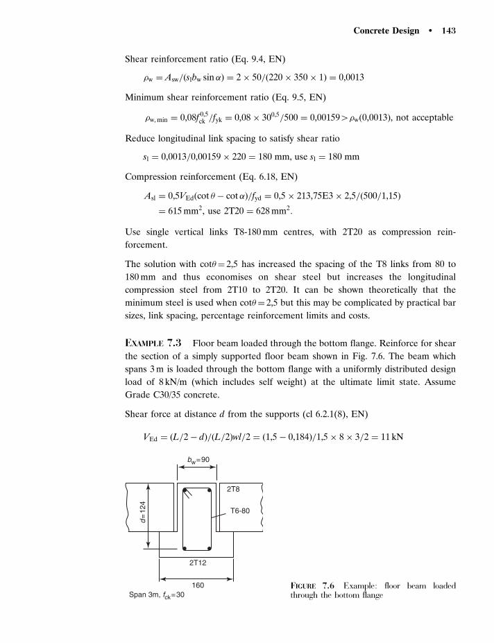
Shear reinforcement ratio (Eq. 9.4, EN)
w ¼ Asw=ðslbw sin �Þ ¼ 2 � 50=ð220 � 350 � 1Þ ¼ 0,0013
Minimum shear reinforcement ratio (Eq. 9.5, EN)
w, min ¼ 0,08f 0,5ck =fyk ¼ 0,08 � 300,5=500 ¼ 0,001594wð0,0013Þ, not acceptable
Reduce longitudinal link spacing to satisfy shear ratio
sl ¼ 0,0013=0,00159 � 220 ¼ 180 mm, use sl ¼ 180 mm
Compression reinforcement (Eq. 6.18, EN)
Asl ¼ 0,5VEdðcot � � cot�Þ=fyd ¼ 0,5 � 213,75E3 � 2,5=ð500=1,15Þ
¼ 615 mm2, use 2T20 ¼ 628 mm2:
Use single vertical links T8-180 mm centres, with 2T20 as compression rein-
forcement.
The solution with cot�¼ 2,5 has increased the spacing of the T8 links from 80 to
180 mm and thus economises on shear steel but increases the longitudinal
compression steel from 2T10 to 2T20. It can be shown theoretically that the
minimum steel is used when cot�¼ 2,5 but this may be complicated by practical bar
sizes, link spacing, percentage reinforcement limits and costs.
EXAMPLE 7.3 Floor beam loaded through the bottom flange. Reinforce for shear
the section of a simply supported floor beam shown in Fig. 7.6. The beam which
spans 3 m is loaded through the bottom flange with a uniformly distributed design
load of 8 kN/m (which includes self weight) at the ultimate limit state. Assume
Grade C30/35 concrete.
Shear force at distance d from the supports (cl 6.2.1(8), EN)
VEd ¼ ðL=2 � dÞ=ðL=2Þwl=2 ¼ ð1,5 � 0,184Þ=1,5 � 8 � 3=2 ¼ 11 kN
160
2T12
bw=90
d=
124
2T8
T6-80
Span 3m, fck=30FIGURE 7.6 Example: floor beam loadedthrough the bottom flange
Concrete Design � 143
Check shear force resistance as a singly reinforced beam (Eq. 6.2a, EN)
VRd,c ¼ ½CRd,ckð100l fckÞ1=3
þ0,15cp�bwd
¼ ½0,18=1,5�2ð100�0,02�30Þ1=3 þ0��90�124=1E3
¼ 10,475VEdð11ÞkN, unsatisfactory and links to resist all of the shear force:
Minimum shear resistance
vmin ¼ 0,035k1,5f 0,5ck ¼ 0,035 � 21,5 � 300,5 ¼ 0,542
Vmin ¼ ðvmin þ k1cpÞbwd
¼ ð0,542 þ 0Þ � 90 � 124=1E3 ¼ 6,055VRd,cð10,47Þ kN, satisfactory:
Depth factor
k ¼ 1 þ ð200=dÞ0,5¼ 1 þ ð200=124Þ0,5
¼ 2,274 2, use k ¼ 2
Longitudinal steel ratio (cl 6.2.2(1), EN)
l ¼ As=ðbwdÞ ¼ 226=ð90 � 124Þ ¼ 0,02, acceptable
Minimum longitudinal steel ratio (cl 9.2.1.1, EN)
l,min ¼ 0,26fctm=fyk ¼ 0,26 � 2,9=500 ¼ 0,00155lð0,02Þ, acceptable:
Shear reinforcement (�¼ 458 and �¼ 908) (Eq. 6.8, EN)
Asw=sl ¼ VEd=ðz fywdÞ ¼ 11E3=ð0,9 � 124 � 0,8 � 500Þ ¼ 0,246 mm
Assuming T6 vertical links, longitudinal spacing
sl ¼ Asw=0,246 ¼ 2 � 28=0,246 ¼ 227,2 mm
Maximum longitudinal spacing of vertical links (Eq. 9.6, EN)
sl, max ¼ 0,75dð1 þ cot �Þ ¼ 0,75 � 124ð1 þ 0Þ ¼ 93 mm, use s1 ¼ 80 mm:
Maximum shear resistance of the concrete (Eq. 6.9, EN)
VRd, max ¼ �cwbwz n fcd=ðcot � þ tan �Þ
¼ 1,0 � 90 � 0,9 � 124 � 0,6 � 30=1,5=ð1 þ 1Þ=1E3
¼ 60,34VEd, maxð12Þ kN acceptable:
Additional area of link required to support load on bottom flange ðsl ¼ 80 mmÞ
AswðextraÞ ¼ ðWs=LÞ=ð fyw=�sÞ ¼ ð24E3 � 80=3E3Þ=ð0,8 � 500Þ ¼ 1,6 mm2
144 � Chapter 7 / Shear and Torsion

Total area of link required (cl 6.2.1(9), EN)
¼ AswðshearÞ þ AswðextraÞ ¼ 0,246 � 80 þ 1,6 ¼ 21,3 mm2:
Single T6 links, Asw¼ 2� 28¼ 564 21,3 mm2, satisfactory.
Shear reinforcement ratio (Eq. 9.4, EN)
w ¼ Asw=ðsbw sin �Þ ¼ 2 � 28=ð80 � 90 � 1Þ ¼ 0,00778
Minimum shear reinforcement ratio (Eq. 9.5, EN)
w,min ¼ 0,08f 0,5ck =fyk ¼ 0,08 � 300,5=500 ¼ 0,00165 wð0,00778Þ, acceptable:
Compression streel required based on shear (Eq. 6.18, EN)
Asl ¼ 0,5VEdðcot � � cot �Þ=fyd ¼ 0,5 � 11E3 � 1=ð500=1,15Þ ¼ 12,65 mm2, use
2T8 ¼ 101 mm2:
Use single vertical links, T6-80, with 2T8 as compression reinforcement (Fig. 7.6).
7.3.5 Shear Resistance of Bent-up Bars
In situations where all the longitudinal tensile reinforcement is not required to resist
the bending moment at the ultimate limit state, some of the bars may be bent-up to
form shear reinforcement (Fig. 7.7). The tensile bars are shown at different levels for
ease in identification, but in practice they are all at the same level as shown in the
cross section. If the tensile reinforcement is used in this way it must be adequately
anchored at the top of the beam to prevent bond failure (See Chapter 8).
Generally, there are insufficient bent-up bars available to resist the total shear force
and vertical links are therefore added. Only a maximum of 50 per cent of the design
shear force (VEd) is allowed (cl 9.2.2(4), EN) to be resisted by the bent-up bars, the
other 50 per cent is to be provided by vertical links. When bent-up bars and vertical
Bent-up bars (b)
V
a abb
V
Two bars (a)
FIGURE 7.7 Bent-up bars
Concrete Design � 145

links are used together their effect is added (Evans, 1967 and Kong, 1978). It should
be appreciated that if tensile bars are bent-up then there is a reduction in tensile
steel, and as a consequence a reduction in bending and shear resistance of the beam.
EXAMPLE 7.4 Beam containing bent-up bars and vertical links. Determine the
shear resistance of the bent-up bars in the beam shown in Fig. 7.8 and add vertical
links to resist a design shear force of VEd ¼ 500 kN. Assume C30/35 Grade concrete.
Stage (1) Shear force resistance as a singly reinforced beam at a section with 2T25
bars (Eq. 6.2a, EN)
VRd,c ¼ ½CRd,ckð100l fckÞ1=3
þ 0,15cp�bwd
¼ ½0,18=1,5� 1,67ð100� 0,00727� 30Þ1=3 þ 0� � 300� 450=1E3
¼ 75,515VEdð500ÞkN, add shear reinforcement to resist all of the
shear force:
Minimum shear force resistance
Vmin ¼ ð0,035k1,5f 0,5ck þ k1cpÞbwd
¼ ð0,035 � 1,671,5 � 300,5 þ 0Þ � 300 � 450=1E3
¼ 55,855VRd,cð75,51Þ kN, acceptable:
Depth factor
k ¼ 1 þ ð200=dÞ0,5¼ 1 þ ð200=450Þ0,5
¼ 1,675 2, acceptable
Tensile reinforcement ratio (cl 6.2.2(1), EN)
1 ¼ As=ðbwdÞ ¼ 982=ð300 � 450Þ ¼ 0,007275 0,02, acceptable
Minimum ratio of longitudinal tensile steel (cl 9.2.1.1, EN)
l,min ¼ 0,26fctm=fyk ¼ 0,26 � 2,9=500 ¼ 0,001515lð0,00727Þ, acceptable:
bw=300
fck=30
2T25
6T25links T12-140
2T25
sb=540
V=500kN
45°
V 2T25
6T25
d=
450
FIGURE 7.8 Example: bent-up bars
146 � Chapter 7 / Shear and Torsion

Stage (2) For bent-up bars with �¼ �¼ 458.
Maximum longitudinal spacing of bent-up bars (Eq. 9.7, EN)
sb,max ¼ 0,6dð1 þ cot �Þ ¼ 0,6 � 450ð1 þ 1Þ ¼ 540 mm, use sb ¼ 540 mm:
Design shear resistance of 2T25 bent-up bars at 458 (Eq. 6.13, EN)
VRd,s ¼ ðAsw=sÞz fywdðcot � þ cot �Þ sin �
¼ ð982=540Þ � 0,9 � 450 � 0,8 � 500ð1 þ 1Þ � 0,707=1E3 ¼ 4174ðVEd=2Þ kN
Add vertical links to resist half of the shear force (Eq. 6.8, EN)
Asw=s ¼ ðVEd=2Þ=ðz fywdÞ ¼ ð500E3=2Þ=ð0,9 � 450 � 0,8 � 500Þ ¼ 1,54 mm
For single T12 vertical links the longitudinal spacing
sl ¼ Asw=1,54 ¼ 2 � 113=1,54 ¼ 147 mm, use sl ¼ 140 mm:
Maximum longitudinal spacing of vertical links (cl 9.2.2(6), EN)
sl,max ¼ 0,75dð1 þ cot �Þ ¼ 0,75 � 450ð1 þ 0Þ ¼ 2704sl ¼ 140 mm:
Check for maximum shear resistance (Eq. 6.9, EN)
VRd, max ¼ �cwbwznfcd=ðcot � þ cot �Þ
¼ 1 � 300 � 0,9 � 450 � 0,6 � ð30=1,5Þ=ð1 þ 1Þ=1E3
¼ 7294VEdð500Þ kN, therefore satisfactory:
Shear reinforcement ratio for vertical links (Eq. 9.4, EN)
w ¼ Asw=ðsbw sin �Þ ¼ 2 � 113=ð140 � 300 � 1Þ ¼ 0,00538
Shear reinforcement ratio for bent-up bars (Eq. 9.4, EN)
w ¼ Asw=ðsbw sin �Þ ¼ 2 � 491=ð540 � 300 � 0,707Þ ¼ 0,00857
Minimum shear reinforcement ratio (Eq. 9.5, EN)
w,min ¼ 0,08f 0,5ck =fyk ¼ 0,08 � 300,5=500 ¼ 0,001595wð0,00538Þ, acceptable:
Maximum effective area of vertical links (Eq. 6.12, EN)
Asw,max fywd=ðbwslÞ ¼ 2 � 113 � 0,8 � 500=ð300 � 140Þ ¼ 2,15 MPa
0,5�cnfcd ¼ 0,5 � 1 � 0,6 � 30=1,5 ¼ 642,15 MPa, therefore satisfactory:
Maximum effective area of inclined bars (Eq. 6.13, EN)
Asw,max fywdz=ðbdslÞðcot�þ cot�Þ sin�¼ 2� 491� 0,8� 500� 0,9=ð300� 540Þ
ð1þ 1Þ � 0,707 ¼ 3,09 MPa
0,5�cnfcdðz=dÞðcot �þ cot�Þ=ð1þ cot2 �Þ ¼ 0,5� 1� 0,6� 30=1,5� 0,9ð1þ 1Þ=ð1þ 1Þ
¼ 5,443,09 MPa, acceptable:
Concrete Design � 147

Compression reinforcement (Eq. 6.18, EN)
Asl ¼ 0,5VEdðcot � � cot�Þ=fyd
¼ 0,5ð500E3=2Þ � ð1 � 0Þ=ð500=1,15Þ
¼ 575 mm2, use 2T25 ¼ 982 mm2:
Balancing half of this longitudinal reinforcement is included in the tension steel.
For a complete design, check that the extra longitudinal steel does not exceed that
required for pure bending (Eq. 6.18, EN), check anchorage for the bent-up bars as
shown in Chapter 8, and check bar diameters and link spacing for control of crack
width.
Use 2T25-540 as bent-up bars, T12-140 mm centres as links with 2T25 as
compression reinforcement (Fig. 7.8).
7.3.6 Horizontal Shear Between Web and Flangefor a ‘T’ Beam (cl 6.2.4, EN)
If a ‘T’ beam is subjected to a change in bending moment along its length then this
produces shear stresses between the flange and the web at sections 1-1 and 1-2.
(Fig. 7.9).
Horizontal design shear stress (Eq. 6.20, EN)
vEd ¼ �Fd=ðhf�xÞ ð7:12Þ
where �Fd is the range in normal force over a distance �x
380
2 22T10
T8-240
100
T8-120
4T16
375
150 FIGURE 7.9 Example: horizontal and verticalshear stresses in a ‘T’ beam
148 � Chapter 7 / Shear and Torsion

A minimum amount of reinforcement must be provided in the form of vertical links.
The shear resistance per unit length of concrete is assumed to be resisted only by the
links and the cracked concrete resistance is zero (Eq. 6.21, EN)
Ast fyd=sf4vEdhf= cot �f ð7:13Þ
Maximum horizontal shear resistance per unit length of concrete reinforced with
links to prevent crushing of the compression struts in the flange (Eq. 6.22, EN)
vEd 5nfcd sin �f cos �f ð7:14Þ
Experiments (Saemann and Washa (1964), Loov and Patnaik (1994)) justify these
expressions.
EXAMPLE 7.5 Horizontal and vertical shear stresses in a ‘T’ beam. Determine the
size and spacing of links for the ‘T’ beam shown in Fig. 7.9. The beam is simply
supported over a span of 6 m and carries a uniformly distributed design load of
136 kN. Assume C30/35 Grade concrete.
Vertical design shear force at a distance d from the support (cl 6.2.1 (8), EN)
VEd ¼ ðL=2 � dÞ=ðL=2ÞVmax ¼ ð1 � 2d=LÞVmax ¼ ð1 � 2 � 375=3E3Þ136=2 ¼ 51 kN
Stage (1) Vertical shear force resistance as a singly reinforced T beam at a section
with 4T16 bars in tension (Eq. 6.2a, EN)
VRd,c ¼ ½CRd,ckð100l fckÞ1=3
þ 0,15cp�bwd
¼ ½0,18=1,5 � 1,73ð100 � 0,0143 � 30Þ1=3 þ 0� � 150 � 375=1E3
¼ 40,895VEd ð51Þ kN, add stirrups to resist all of the shear force:
Minimum shear force resistance
Vmin ¼ ð0,035k1,5f 0,5ck þ k1cpÞbwd
¼ ð0,035 � 1,731,5 � 300,5 þ 0Þ � 150 � 375=1E3
¼ 24,55VRd,cð40,89Þ kN, acceptable:
Depth factor
k ¼ 1 þ ð200=dÞ0,5¼ 1 þ ð200=375Þ0,5
¼ 1,735 2, acceptable
Tensile reinforcement ratio (cl 6.2.2(1), EN)
pl ¼ As=ðbwdÞ ¼ 804=ð150 � 375Þ ¼ 0,01435 0,02, acceptable:
Minimum ratio of longitudinal tensile steel (cl 9.2.1.1, EN)
l,min ¼ 0,26fctm=fyk ¼ 0,26 � 2,9=500 ¼ 0,00155 plð0,0143Þ, acceptable:
Concrete Design � 149

Stage (2) Combine reinforcement to resist vertical shear stress in the web and
horizontal shear stresses on plane 1-1 (Fig. 7.9)
Change in normal force in the flange over a distance L/4 at the end of the beam
(Eq. 6.20, EN)
�Fd ¼ ðwL2=8 � wL2=32Þ=d ¼ 3=4W
Shear stress on horizontal failure plane 1-1 (Fig. 7.9)
vEd ¼ ð3=4W Þ=ðbwzÞ ¼ ð3=4 � 136E3Þ=ð150 � 0,9 � 375Þ ¼ 2,01 MPa
Shear stress on the vertical plane
vEd ¼ VEd=ðbwdÞ ¼ 51E3=ð150 � 375Þ ¼ 0,907 MPa
Spacing of T8 single vertical links (�¼ 458 and �¼ 908) to resist horizontal shear
stresses
sl ¼ Asf fyd=ðvEdbwÞ
¼ 2 � 50 � 0,8 � 500=ð2,01 � 150Þ ¼ 133 mm, use sl ¼ 120 mm:
Check crushing of the compression strut in the flange, cot�f¼ 1 (Eq. 6.22, EN)
vEd5nfcd sin �f cos �f ¼ 0,6 � 30=1,5 � 0,707 � 0,707 ¼ 642,01 MPa, acceptable:
Maximum longitudinal spacing of vertical links (Eq. 9.6, EN)
sl,max ¼ 0,75dð1 þ cot�Þ ¼ 0,75 � 375 � ð1 þ 0Þ ¼ 2815 300 mm, use sl ¼ 120 mm:
Shear reinforcement ratio (Eq. 9.4, EN)
w ¼ Asw=ðs bw sin �Þ ¼ 2 � 50=ð120 � 150 � 1Þ ¼ 0,0056
Minimum shear reinforcement ratio (Eq. 9.5, EN)
w,min ¼ 0,08f 0,5ck =fyk ¼ 0,08 � 300,5=500 ¼ 0,001595 wð0,0056Þ, satisfactory:
Compression reinforcement (Eq. 6.18, EN)
Asl ¼ 0,5VEdðcot � � cot�Þ=fyd ¼ 0,5 � 51E3 � ð1 � 0Þ=ð500=1,15Þ
¼ 58,65 mm2, use 2T10 ¼ 157 mm2:
Stage (3) Consider the two vertical shear failure planes 1-2 (Fig. 7.9). The change in
normal force in the flange over a length L/4 at the end of the beam (cl 6.2.4(3), EN)
�Fd ¼ ðwL2=8 � wL2=32Þ=d
150 � Chapter 7 / Shear and Torsion
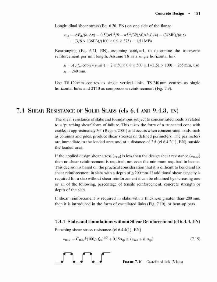
Longitudinal shear stress (Eq. 6.20, EN) on one side of the flange
vEd ¼ �Fd=ðhf�xÞ ¼ 0,5½ðwL2=8 � wL2=32Þ=d�=ðhfL=4Þ ¼ ð3=8W Þ=ðhfzÞ
¼ ð3=8 � 136E3Þ=ð100 � 0,9 � 375Þ ¼ 1,51 MPa
Rearranging (Eq. 6.21, EN), assuming cot�f¼ 1, to determine the transverse
reinforcement per unit length. Assume T8 as a single horizontal link
sf ¼ Asf fyd cot �f=ðvEdhfÞ ¼ 2 � 50 � 0,8 � 500 � 1=ð1,51 � 100Þ ¼ 265 mm, use
sf ¼ 240 mm:
Use T8-120 mm centres as single vertical links, T8-240 mm centres as single
horizontal links and 2T10 as compression reinforcement (Fig. 7.9).
7.4 SHEAR RESISTANCE OF SOLID SLABS (cls 6.4 AND 9.4.3, EN)
The shear resistance of slabs and foundations subject to concentrated loads is related
to a ‘punching shear’ form of failure. This takes the form of a truncated cone with
cracks at approximately 308 (Regan, 2004) and occurs when concentrated loads, such
as columns and piles, produce shear stresses on defined perimeters. The perimeters
are immediate to the loaded area and at a distance of 2 d (cl 6.4.2(1), EN) outside
the loaded area.
If the applied design shear stress (vEd) is less than the design shear resistance (vRd,c)
then no shear reinforcement is required, not even the minimum required in beams.
This decision is based on the practical consideration that it is difficult to bend and fix
shear reinforcement in slabs with a depth of� 200 mm. If additional shear capacity is
required for a slab without shear reinforcement it can be obtained by increasing one
or all of the following, percentage of tensile reinforcement, concrete strength or
depth of the slab.
If shear reinforcement is required in slabs with a thickness greater than 200 mm,
then it is introduced in the form of castellated links (Fig. 7.10), or bent-up bars.
7.4.1 Slabs and Foundations without Shear Reinforcement (cl 6.4.4, EN)
Punching shear stress resistance (cl 6.4.4(1), EN)
vRd,c ¼ CRd,ckð100l fckÞ1=3
þ 0,15cp � ðvmin þ k1cpÞ ð7:15Þ
FIGURE 7.10 Castellated link (5 legs)
Concrete Design � 151
where
CRd,c ¼ 0,18=�c
Minimum shear resistance
ðvmin þ k1cpÞ ¼ 0,035k1,5f 0,5ck þ k1cp
Depth factor
k ¼ 1 þ ð200=dÞ0,5� 2
Longitudinal tensile reinforcement ratio
l ¼ ðly lzÞ0,5
� 0,02
These expressions are similar to those for singly reinforced beams except for the
tensile reinforcement ratio, which is for steel in both directions.
7.4.2 Slabs or Foundations with Shear Reinforcement (cl 6.4.5, EN)
For slabs of thickness greater than 200 mm which are subject to concentrated loads,
where shear reinforcement is required, links are used in castellated form (Fig. 7.10),
or bent-up bars. The shear resistance is part concrete and part steel shear
reinforcement for a perimeter of length u1.
Shear stress resistance of a slab with shear reinforcement in the form of links
(Eq. 6.52, EN)
vRd,cs ¼ 0,75vRd,c þ 1,5ðd=srÞAswfywd,efð1=ðu1dÞÞ sin � ð7:16Þ
where
sr is the radial spacing of perimeters of shear reinforcement (mm) and
fywd,ef ¼ 250þ 0,25d� fywd MPa.
It should be noted that part of the applied design shear stress is resisted by the
concrete and part by the steel. This is in contrast to singly reinforced beams with
shear reinforcement where all of the applied design shear stress is resisted by the
shear reinforcement.
The design process for a concentrated column load consists of making checks for
shear resistance at a basic control perimeters (Fig. 7.11). The first perimeter
is around the loaded area, the second 2 d from the loaded area, and then usually
at successive perimeters at increments of 2 d until shear reinforcement is no
152 � Chapter 7 / Shear and Torsion

longer required. Critical second perimeters for various shapes of loaded areas are
shown in cl 6.4.2(1), EN.
EXAMPLE 7.6 Flat slab subjected to a concentrated load. Check the flat slab
shown in Fig. 7.12 for shear failure. The internal column design load N¼ 1000 kN
and the concrete slab is 300 mm deep, with d¼ 250 mm, and reinforced with T16-
200 mm centres in both directions at the top and bottom of the slab. Assume Grade
C30/35 concrete.
Stage (1) At the column face for an interior column, �¼ 1,15 (cl 6.4.3(6), EN), the
applied punching design shear stress in the slab (Eq. 6.53, EN)
vEd ¼ �VEd=ðuodÞ ¼ 1,5 � 1000E3=ð4 � 400 � 250Þ ¼ 2,88 MPa:
Maximum shear stress resistance allowed at the column face (Eq. 6.53, EN)
vRd, max ¼ 0,5nfcd ¼ 0,5 � 0,528 � 30=1,5 ¼ 5,284 vEdð2,88ÞMPa acceptable,
where strength reduction factor (Eq. 6.6, EN)
v ¼ 0,6ð1 � fck=250Þ ¼ 0,6ð1 � 30=250Þ ¼ 0,528:
2d 2d
FIGURE 7.11 Shear failure of a slab subjected to a concentrated column load
1400
400
Top and bottom reinf. T16-180fck = 30
FIGURE 7.12 Example: slab with aconcentrated load
Concrete Design � 153
Stage (2) Applied design shear stress in the slab for perimeter 2 d from the column
face
vEd ¼ �VEd=ðu1dÞ ¼ 1,15 � 1000E3=ð4 � ð400 þ 4 � 250Þ � 250Þ ¼ 0,821 MPa:
Shear stress resistance without shear reinforcement (Eq. 6.47, EN)
vRd,c ¼CRd,ckð100l fckÞ1=3
þ 0,15cp ¼ 0,18=1,5� 1,89� ð100� 0,00446� 30Þ1=3 þ 0
¼ 0,5385vEdð0,821ÞMPa,
therefore shear reinforcement required.
Minimum shear resistance
ðvmin þ k1cpÞ ¼ 0,035k1,5f 0,5ck þ k1cp ¼ 0,035 � 1,891,5 � 300,5 þ 0
¼ 0,365 vRd,cð0,538ÞMPa, acceptable:
Depth factor
k ¼ 1 þ ð200=dÞ0,5¼ 1 þ ð200=250Þ0,5
¼ 1,8952:
Tensile reinforcement ratio (cl 6.4.4, EN)
l ¼ ðly lzÞ0,5
¼ 1115=ð1E3 � 250Þ ¼ 0,0044650,02, acceptable:
Shear stress resistance with vertical links (T10-180) (Eq. 6.52, EN)
vRd,cs ¼ 0,75vRdc þ 1,5ðd=srÞ Aswfywd,efð1=ðu1dÞÞ sin �
¼ 0,75 � 0,538 þ 1,5 � ð250=180Þ � 12 � 79 � 312,5=
ð4 � ð400 þ 4 � 250Þ � 250Þ � 1
¼ 0,8464 vEdð0,821ÞMPa, acceptable
where
fywd,ef ¼ 250 þ 0,25d ¼ 250 þ 0,25 � 250 ¼ 312,55 fywdð0,8 � 500ÞMPa:
Minimum area of a link leg with sr ¼ st ¼ 180 mm (cl 9.4.3(2), EN)
Asw, minð1,5 sin �þ cos �Þ=ðsrstÞ ¼ 79 � ð1,5 � 1 þ 0Þ=ð180 � 180Þ ¼ 0,00366
0,08f 0,5ck =fyk ¼ 0,08 � 300,5=500 ¼ 0,0008255 0,00366, acceptable:
Repeat calculations at increasing radii until the control perimeter at which shear
reinforcement is not required (Eq. 6.54, EN). Details of punching shear
reinforcement are given in cl 9.4.3, EN.
uout,ef ¼ �VEd=ðvRd,cdÞ ¼ 1,15 � 1000E3=ð0,538 � 250Þ ¼ 8550 mm:
154 � Chapter 7 / Shear and Torsion

7.4.3 Shear Resistance of a Column Base without Shear Reinforcement(cl 6.4.4, EN)
The design of a pad foundation for shear is similar to that for concentrated loads on
slabs. Checks for punching shear resistance are made at control perimeters within 2d
from the column face (cl 6.4.4(2), EN). The lowest value controls the design. Similar
criteria are used to decide whether shear reinforcement is necessary. Often, in pad
foundations, the depth of the foundation is increased rather than introduce shear
reinforcement.
EXAMPLE 7.7 Shear resistance of pad foundation. Design for shear the pad
foundation shown in Fig. 7.13. The steel required to resist the bending moment is
shown. Assume C20/25 Grade of concrete.
Stage (1) Perimeter at the face of the column
Bending moment at the column face increases the shear stress factor (Eqs. 6.39 and
6.51, EN)
� ¼ 1 þ kMEdu1=ðVEd,redW1Þ
¼ 1 þ 0,6 � 3333E6 � 4E3=ð6500E3 � 81,67E6Þ ¼ 1,015
c1=c2 ¼ 1 and hence k ¼ 0,6 ðTable 6:1, ENÞ
From Eq. 6.41, EN
W1 ¼ c21=2 þ c1c2 þ 4c2dþ 16d2 þ 2 dc1
¼ 0,5 þ 1 þ 4 � 1 � 1,94 þ 16 � 1,942 þ 2 � 1,94 � 1 ¼ 81; 67 m2:
Applied design punching shear stress at the face of the column (Eq. 6.38, EN)
vEd ¼ �VEd=ðuidÞ ¼ 1,015 � 6500E3=ð4E3 � 1,94E3Þ ¼ 0,85 MPa:
10 m
90 150 170 kN/m2
N = 6500 kN
d =
1,9
4m
Mt = 3333 kNm
fck = 20 d1 m
a a
width 5 mT32-80 in both directions
FIGURE 7.13 Example: a padfoundation
Concrete Design � 155

Maximum shear stress allowed (Eq. 6.53, EN)
vRd, max ¼ 0,5vfcd ¼ 0,5 � 0,552 � 20=1,5 ¼ 3,684 vEdð0,85ÞMPa, acceptable,
where the strength reduction factor (Eq. 6.6, EN)
v ¼ 0,6ð1 � fck=250Þ ¼ 0,6ð1 � 20=250Þ ¼ 0,552
Stage (2) The 2 d perimeter lies outside the base. Check a section across the base
at a distance d from the face of the column.
Shear stress resistance of a singly reinforced base at a section distance d from the
face of the column (Eq. 6.50, EN).
vRd,c ¼ CRd,ckð100l fckÞ1=3
� 2d=a
¼ 0,18=1,5 � 1,32ð100 � 0,00518 � 20Þ1=3 � 2 ¼ 0,345 � 2 ¼ 0,69 MPa:
Minimum shear stress resistance
vminð2 d=aÞ ¼ 0,035k1,5f 0,5ck ð2d=aÞ
¼ 0,035 � 1,321,5 � 200,5 � 2 ¼ 0,3765vRd,cð0,69ÞMPa, acceptable:
Depth factor
k ¼ 1 þ ð200=dÞ0,5¼ 1 þ ð200=1940Þ0,5
¼ 1,3252:
Tensile reinforcement ratio (cl 6.4.4, EN)
l ¼ ðly lzÞ0,5
¼ 10053=ð1E3 � 1940Þ ¼ 0,005185 0,02, acceptable:
To determine the applied shear stress at a distance d from the column face use the
soil pressure diagram (Fig. 7.13).
Pressure on the ground at toes of foundation
p ¼ 6500=ð10 � 5Þ � 3333=ð5 � 102=6Þ ¼ 130 � 40 ¼ þ170 and þ 90 kN=m2:
Pressure at a distance d from the column face
p ¼ 90 þ ð5 þ B=2 þ dÞ=10 � ð170 � 90Þ ¼ 150 kN=m2:
Applied design shear force at the critical section across the full width of the base
VEd ¼ 2,5 � 5 � ð170 þ 150Þ=2 ¼ 2000 kN:
Design shear stress
vEd ¼ VEd=ðudÞ ¼ 2000E3=ð5E3 � 1,94E3Þ ¼ 0,2065 vRd,cð0,69Þ MPa acceptable:
156 � Chapter 7 / Shear and Torsion

Alternatively calculate the applied design shear stress from (Eq. 6.51, EN)
vEd ¼ VEd=ðudÞð1þ kMEdu=VEdW Þ
¼ 6500E3=ð2� 5E3� 1,94E3Þð1þ 0,6� 3333E6� 2� 5E3=ð6500E3� 81,67E6ÞÞ
¼ 0,335� ð1þ 0,0377Þ ¼ 0,3485vRd,cð0,69ÞMPa also satisfactory:
This applied design shear stress (0,348 MPa) is considerably higher than previously
(0,206 MPa) and is therefore more conservative.
Maximum punching shear stress resistance (Eq. 6.53, EN)
vRd, max ¼ 0,5nfcd ¼ 0,5 � 0,6ð1 � 20=250Þ � 20=1,5
¼ 3,684 vEdð0,206Þ MPa, satisfactory:
Stage (3) Check bond length (a-a) (Fig. 7.13) (cl 9.8.2.2, EN).
Force in the tensile reinforcement (Eq. 9.13, EN)
Fs ¼ R ze=zi ¼ 1600 � 3,847=ð0,9 � 1,94Þ ¼ 3195 kN
where
e ¼ M=N ¼ 3333=6500 ¼ 0,513 m
R ¼ 160 � 2 � 5 ¼ 1600 kN ðapprox:Þ
ze ¼ 5 � e� 1 ¼ 5 � 0,513 � 1 ¼ 3,487 m
sd ¼ Fs=As ¼ 3195E3=ð5E3=80 � 804Þ ¼ 63,6 MPa:
Bond length required (Eq. 8.3, EN)
lb,req ¼ ð�=4Þðsd=fbdÞ ¼ ð32=4Þ � ð63,6=2,25Þ ¼ 226 mm:
Design value of the bond stress (Eq. 8.2, EN)
fbd ¼ 2,25fctk,0,5=�c ¼ 2,25 � 1,5=1,5 ¼ 2,25 MPa:
Design anchorage length (Eq. 8.4, EN)
lbd ¼ �1�2�3�4lb,req ¼ 0,7 � 226 ¼ 158 mm:
Bond length available
¼ 2000 � cover ¼ 2000 � 50 ¼ 19504 lbdð158Þmm, acceptable:
The procedure should be repeated at other perimeters to check whether there is one
more critical. The magnitude of the applied shear stress (vEd¼ 0,206 MPa) could be
Concrete Design � 157
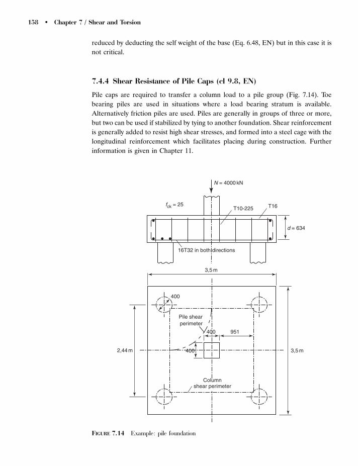
reduced by deducting the self weight of the base (Eq. 6.48, EN) but in this case it is
not critical.
7.4.4 Shear Resistance of Pile Caps (cl 9.8, EN)
Pile caps are required to transfer a column load to a pile group (Fig. 7.14). Toe
bearing piles are used in situations where a load bearing stratum is available.
Alternatively friction piles are used. Piles are generally in groups of three or more,
but two can be used if stabilized by tying to another foundation. Shear reinforcement
is generally added to resist high shear stresses, and formed into a steel cage with the
longitudinal reinforcement which facilitates placing during construction. Further
information is given in Chapter 11.
N = 4000 kN
fck = 25
d = 634
T10-225 T16
16T32 in both directions
3,5 m
3,5 m
400
400
400
Columnshear perimeter
951
2,44 m
Pile shearperimeter
FIGURE 7.14 Example: pile foundation
158 � Chapter 7 / Shear and Torsion

EXAMPLE 7.8 Shear resistance of a pile cap. Check the pile cap shown in Fig. 7.14
for shear resistance and reinforce if necessary. Assume an internal column and
Grade C25/30 concrete.
Stage (1) Check for punching shear failure round the column.
Applied shear stress at column perimeter (Eq. 6.53, EN)
vEd ¼ �VEd=ðuidÞ ¼ 1,15 � 4000E3=ð4 � 400 � 634Þ ¼ 4,53 MPa:
Maximum shear stress resistance (Eq. 6.5, EN)
vRd, max ¼ 0,5nfcd ¼ 0,5 � 0,6ð1 � 25=250Þ � 25=1,5 ¼ 4,554,53 MPa, acceptable:
Applied design shear stress round shear perimeter (Fig. 7.14)
vEd ¼ 4000E3=ð4 � ð2 � 951 þ 400Þ � 634Þ ¼ 0,685 MPa:
Shear stress resistance singly reinforced (Eq. 6.50, EN).
vRd,c ¼ CRd,ckð100l fckÞ1=3
� 2 d=a
¼ 0,18=1,5 � 1,56ð100 � 0,0058 � 25Þ1=3 � 2 � 634=951
¼ 0,6085 vEdð0,685Þ MPa,
therefore shear reinforcement required.
vmin ¼ 0,035k1,5f 0,5ck � 2d=a ¼ 0,035 � 1,561,5 � 200,5 � 1,33
¼ 0,4555vRd,cð0,608ÞMPa, satisfactory:
Depth factor
k ¼ 1 þ ð200=dÞ0,5¼ 1 þ ð200=634Þ0,5
¼ 1,565 2:
Reinforcement ratio (cl 6.4.4(1), EN)
l ¼ ðly lzÞ0,5
¼ 16 � 804=ð3500 � 634Þ ¼ 0,005185 0,02, satisfactory:
Shear stress resistance of T12 vertical links assuming a radial spacing sr ¼ 225 mm
(Eq. 6.52, EN)
vRd,cs ¼ 0,75VRd,c þ 1,5ðd=srÞ Aswfywd,efð1=ðu1dÞÞ sin �
¼ 0,75 � 0,608 þ 1,5 � ð634=225Þ � 4 � 3 � 113 � 400=
ð4ð400 þ 2 � 951Þ � 634Þ � 1
¼ 0,8494 vEdð0,685Þ MPa satisfactory:
fywd,ef ¼ 250 þ 0,25d ¼ 250 þ 0,25 � 634 ¼ 408,540,8 � 500 ¼ 400 MPa, use
fywd,ef ¼ 400 MPa:
Maximum longitudinal spacing of the vertical links (Eq. 9.6, EN)
sl, max ¼ 0,75dð1 þ cot�Þ ¼ 0,75 � 634 ¼ 475,54 225 mm, satisfactory:
Concrete Design � 159

Shear reinforcement ratio (Eq. 9.4, EN)
w ¼ Asw=ðs bw sin �Þ ¼ 4 � 3 � 113=ð225 � 4 � 400 � 1Þ ¼ 0,00377:
Minimum shear reinforcement ratio (Eq. 9.5, EN)
w, min ¼ 0,08f 0,5ck =fyk ¼ 0,08 � 250,5=408,5 ¼ 0,000985 wð0,00377Þ, acceptable
Stage (2) Check for shear resistance round a pile.
Applied punching shear stress round a pile at edge of slab (Eq. 6.53, EN)
vEd ¼ �VEd=ðu dÞ ¼ 1,5 � 1000E3=ð � 400 � 634Þ ¼ 1,88 MPa:
Maximum shear stress resistance (Eq. 6.5, EN)
vRd, max ¼ 0,5nfcd ¼ 0,5� 0,6ð1� 25=30Þ� 25=1,5 ¼ 4,54vEdð1,88Þ MPa acceptable:
Applied shear stress at the pile shear perimeter (Fig. 7.14)
vEd ¼ �VEd=ðu dÞ ¼ 1,5 � 1000E3=½ð2 � 530 þ =4 � 1220Þ � 634� ¼ 1,17 MPa:
Shear stress resistance (see previous calculations) vRd,c ¼ 0,6085vEdð1,17Þ MPa
therefore shear reinforcement required.
Shear stress resistance with link T12-225 (Eq. 6.52, EN)
vRd,cs ¼ 0,75VRdc þ1,5ðd=srÞAswfywd,efð1=ðu1dÞÞsin�
¼ 0,75�0,608þ1,5�ð634=225Þ�3�4�113�400=ð1220ð2þ =2Þ�634Þ�1
¼ 1,294vEdð1,17Þ MPa, acceptable:
7.4.5 Corbels (cl J3, Figs 6.4 (b) and 6.6, EN)
Corbels are brackets on columns supporting loads as shown in Fig. 7.15. Generally
the ratio ac/d5 2 and the shear resistance is enhanced. Design consists in checking
for combined shear force and bending moment, and bond lengths. See also
Section 8.4.7.
EXAMPLE 7.9 Design of a corbel. Reinforce the corbel (Fig. 7.15(a)) for the
design loads shown. Assume C30/40 Grade concrete.
Ratio
ac=hc ¼ 160=300 ¼ 0,5340,5, therefore use vertical links (see Fig. J6(b), EN).
160 � Chapter 7 / Shear and Torsion

Stage (1) Force in the tension steel from moments of forces about A
Fld ¼ bending þ horizontal force þ shear ¼ VEdac=zþHEd þ 0,5VEd
¼ 60 � 160=ð0,9 � 270Þ þ 0,2 � 60 þ 0,5 � 60 ¼ 81,5 kN:
Area of steel required to resist the force Fld
As ¼ Fld=fyd ¼ 81,5E3=ð500=1,15Þ ¼ 187,5 mm2, use 2T12 ¼ 226 mm2:
300
300
A
300
100
2T10
2T12
2T20
2T20
T8-50
Column reinforcement is not shown
lb
lb
bw = 200
ac=160
HEd=12 kN
VEd=60 kN
av
h c=
300
lb
50 50
d d
160
100
300
60
c c
b
25 60
160
100
b
(a)
(b)
(c)(d)
FIGURE 7.15 Example: design of a corbel
Concrete Design � 161

Minimum area of mild steel (cl 9.2.1.1, EN)
0,26ð fctm=fykÞbtd ¼ 0,26 � ð2,9=500Þ � 200 � 270 ¼ 81,55226 mm2
0,0013btd ¼ 0,0013 � 200 � 270 ¼ 705226 mm2, acceptable:
Stage (2) Reduced applied shear stress for small values of shear/span ratio
(cl 6.2.2(6), EN)
av=ð2dÞ ¼ ð160 � 50Þ=ð2 � 270Þ ¼ 0,204
vEd ¼ 60E3ð1 � av=ð2dÞÞ=ðb dÞ ¼ 60E3ð1 � ð160 � 50Þ=ð2 � 270ÞÞ=ð200 � 270Þ
¼ 0,885 MPa:
Shear stress resistance without shear reinforcement (Eq. 6.2a, EN)
vRd,c ¼CRd,ckð100l fckÞ1=3
þ 0,15cp
¼ 0,18=1,5� 1,86ð100� 0,00418� 30Þ1=3 � 0,15� 0,2 ¼ 0,4885vEdð0,885ÞMPa,
therefore links required.
Minimum shear stress resistance
ðvmin þ k1cpÞ ¼ 0,035k1,5f 0,5ck þ k1cp ¼ 0,035 � 1,561,5 � 250,5 � 0,15 � 0,2
¼ 0,3115 0,488 MPa, acceptable:
Depth factor
k ¼ 1 þ ð200=dÞ0,5¼ 1 þ ð200=270Þ0,5
¼ 1,865 2:
Tensile reinforcement ratio
1 ¼ As=ðbwdÞ ¼ 226=ð200 � 270Þ ¼ 0,00418
cp ¼ 12E3=ð200 � 300Þ ¼ 0,2 MPa
0,2fcd ¼ 0,2 � 30=1,5 ¼ 4 4 0,2 MPa, satisfactory:
Shear stress resistance with single T8-50 vertical links (Eq. 6.19, EN)
vRs ¼ Aswð0,75av=sÞfywd sin �=ðbwdÞ
¼ 2 � 50 � 0,75 � ðð160 � 50Þ=50Þ � 0,8 � 500=ð200 � 270Þ
¼ 1,224 vEdð0,885ÞMPa, acceptable:
Maximum shear stress resistance (Eq. 6.5, EN)
vRd, max ¼ 0,5nfcd ¼ 0,5 � 0,528 � 30=1,5 ¼ 5,284 vEd, max ð1,11Þ MPa, acceptable:
Strength reduction factor (Eq. 6.6, EN)
v ¼ 0,6ð1 � fck=250Þ ¼ 0,6ð1 � 30=250Þ ¼ 0,52840,5:
162 � Chapter 7 / Shear and Torsion

Shear reinforcement ratio (Eq. 9.4, EN)
w ¼ Asw=ðs bw sin �Þ ¼ 2 � 50=ð50 � 200 � 1Þ ¼ 0,01:
Minimum shear reinforcement (Eq. 9.5, EN)
w, min ¼ 0,08f 0,5ck =fyk ¼ 0,08 � 300,5=500 ¼ 0,000875wð0,01Þ, acceptable:
Maximum spacing of links (Eq. 9.6, EN)
smax ¼ 0,75dð1 þ 0Þ ¼ 0,75 � 270 ¼ 203 4 sð50Þmm, therefore satisfactory:
Compression reinforcement (Eq. 6.18, EN)
Asl ¼ 0,5VEdðcot � � cot�Þ=fyd ¼ 0,5 � 60E3 � 1=ð500=1,15Þ ¼ 16,6 mm2, use
2T10 ¼ 157 mm2:
Stage (3) Bond length (b-b) required for tension bars (2T20) end of beam
(Fig. 7.15(b)). Axial stress in reinforcement
sd ¼ ðHEd þ 0,5VEdÞ=As ¼ ð12E3 þ 0,5 � 60E3Þ=628 ¼ 67 MPa:
Basic anchorage length required (Eq. 8.3, EN)
lb,req ¼ ð�=4Þðsd=fbdÞ ¼ ð20=4Þ � ð67=3Þ ¼ 112 mm:
Design value of the bond stress (Eq. 8.2, EN)
fbd ¼ 2,25fctk,0,5=�c ¼ 2,25 � 2=1,5 ¼ 3 MPa:
Design anchorage length (Eq. 8.4, EN)
lbd ¼ �1�2�3�4lb,req ¼ 0,7 � 112 ¼ 78 mm:
Bond length available
ac þ 50� clearance� cover ¼ 160þ 50� 25� 60 ¼ 1254 lbdð78Þmm, acceptable:
Bond length (c-c) required for tension bars (2T12) at end of the bracket
(Fig. 7.15(c)). Axial stress in reinforcement
sd ¼ ðAs,req=AsÞfyd ¼ ð187,5=226Þ � ð500=1,5Þ ¼ 277 MPa:
Basic anchorage length required (Eq. 8.3, EN)
lb,req ¼ ð�=4Þðsd=fbdÞ ¼ ð12=4Þ � ð277=3Þ ¼ 277 mm:
Concrete Design � 163
Design value of the bond stress (Eq. 8.2, EN)
fbd ¼ 2,25fctk,0,5=�c ¼ 2,25 � 2=1,5 ¼ 3 MPa:
Design anchorage length (Eq. 8.4, EN)
lbd ¼ �1�2�3�4lb,req ¼ 0,7 � 277 ¼ 194 mm:
Bond length available¼ 300� 160þ 50¼ 190¼ lbd (194) mm approx. acceptable.
Bond length (d-d) required for tension bars (2T12) embedded in the column
(Fig. 7.15(d)). Axial stress in reinforcement
sd ¼ ðAs,req=AsÞfyd ¼ ð187,5=226Þ � ð500=1,5Þ ¼ 277 MPa:
Bond length required (Eq. 8.3, EN)
lb,req ¼ ð�=4Þðsd=fbdÞ ¼ ð12=4Þ � ð277=3Þ ¼ 277 mm:
Design value of the bond stress (Eq. 8.2, EN)
fbd ¼ 2,25fctk,0,5=�c ¼ 2,25 � 2=1,5 ¼ 3 MPa:
Design anchorage length (Eq. 8.4, EN)
lbd ¼ �1�2�3�4lb,req ¼ 0,7 � 277 ¼ 194 mm:
Bond length available
¼ h� 2 � cover ¼ 300 � 2 � 50 ¼ 2004 lbdð194Þ mm, acceptable:
An alternative method of design for corbels using a strut and tie model is given
in cl J3, EN.
7.5 SHEAR RESISTANCE OF PRESTRESSED CONCRETE BEAMS
(cls 6.2.2 AND 6.2.3 EN)
7.5.1 Introduction
The modes of shear failure and design requirements for prestressed beams are
similar to those for reinforced concrete. Prestressing and increased concrete strength
delays the formation of cracks and increases shear resistance. However the lower
percentage of tensile reinforcement reduces the shear resistance. There are two
situations to check. The first is as for a singly reinforced section at a section where
164 � Chapter 7 / Shear and Torsion

there are bending cracks. The second is where there are no bending cracks but the
principal tensile stress in the web is high.
EXAMPLE 7.10 Shear resistance of a pretensioned beam. Design for shear at the
ultimate limit state the pretensioned prestressed concrete beam shown in Fig. 7.16.
The beam is simply supported over a span of 10 m and carries a uniformly
distributed design load of 160 kN at the ultimate limit state. The beam has been
designed to meet the requirements for bending. Assume the prestressing force is
transferred when the concrete strength is Grade C30/40 and is mature at concrete
Grade C50/60. The area of prestressing steel is 645 mm2 with an initial prestressing
force of 1000 kN with 20 per cent losses, and 7 mm wires stressed to 1550 MPa.
Stage 1 Check as a cracked singly reinforced concrete beam.
Determine the section closest to the support at a distance x where cracking occurs
at the bottom of the beam.
Bending stress¼ effective prestressþ concrete tensile strength
0,5wL xð1 � x=LÞ=Z ¼ Pe=Aþ Pee=Zþ fctm=�c
0,5 � 16 � 10E3xð1 � x=10E3Þ=20,4E6
¼ 800E3=135E3 þ 800E3 � 160=20,4E6 þ 4,1=1,5
x2 � 16E3xþ 30464E3 ¼ 0
x ¼ 2209 mm from the support:
where
A ¼ BD� bd ¼ 400 � 600 � 300 � 350 ¼ 135E3 mm2
I ¼ BD3=12 � bd3=12 ¼ ð400 � 6003 � 300 � 3503Þ=12 ¼ 6128E6 mm4
Z ¼ I=ðD=2Þ ¼ 6128E6=300 ¼ 20,4E6 mm3
Design shear force at 2,209 m from the support
VEd ¼ ð5 � 2,209Þ=5 � 80 ¼ 44,66 kN
400
460
100
100
100
150 500
10 m
300
50
50P
CL
FIGURE 7.16 Example: shear resistance of a prestressed beam
Concrete Design � 165
and the design shear stress
vEd ¼ VEd=ðbwdÞ ¼ 44,66E3=ð100 � 460Þ ¼ 0,97 MPa:
Shear stress resistance of section without shear reinforcement (Eq. 6.2a, EN)
vRd,c ¼ CRd,ckð100l fckÞ1=3
þ 0,15cp
¼ 0,18=1,5 � 1,66ð100 � 0,014 � 50Þ1=3 þ 0,15 � 5,93 ¼ 1,714 vEdð0,97ÞMPa
where
cp ¼ NEd=Ac ¼ 800E3=135E3 ¼ 5,93 MPa
0,2fcd ¼ 0,2 � 50=1,5 ¼ 6,674cpð5,93Þ MPa satisfactory:
Depth factor
k ¼ 1 þ ð200=dÞ0,5¼ 1 þ ð200=460Þ0,5
¼ 1,6652:
Longitudinal tensile reinforcement ratio (cl 6.2.2(1), EN)
l ¼ 645=ð100 � 460Þ ¼ 0,01450,02, satisfactory:
Minimum shear stress resistance
ðvmin þ k1cpÞ ¼ 0,035k1,5f 0,5ck þ 0,15 � 5,93
¼ 0,035 � 1,661,5 � 500,5 þ 0,15 � 5,93
¼ 1,425 vRd,cð1,71ÞMPa, acceptable:
Add minimum shear reinforcement (cl 6.2.1(4), EN).
Minimum shear ratio (Eq. 9.5, EN)
w,min ¼ 0,08f 0,5ck =fyk ¼ 0,08 � 500,5=500 ¼ 0,00113:
Longitudinal spacing for single T8 vertical links (Eq. 9.4, EN)
sl ¼ Asw=ðw, minbwÞ ¼ 2 � 50=ð0,00113 � 100Þ ¼ 885 mm:
Maximum longitudinal spacing of vertical links (Eq. 9.6, EN)
sl,max ¼ 0,75dð1 þ cot�Þ ¼ 0,75 � 460ð1 þ 0Þ ¼ 345, use sl ¼ 340 mm
Maximum shear force resistance of T8-340 vertical links (Eq. 6.8, EN)
VRd,s ¼ ðAsw=sÞz fywd ¼ ð2 � 50=340Þ � 0,9 � 460 � 0,8 � 500=1E3
¼ 48,74VEdð44,66Þ kN, acceptable:
166 � Chapter 7 / Shear and Torsion
Maximum shear force resistance of the concrete (Eq. 6.9, EN)
05 cpð5,93Þ5 0,25fcdð8,33ÞMPa
�cw ¼ 1 þ cp=fcd ¼ 1 þ 5,93=ð50=1,5Þ ¼ 1,18
VRd, max ¼ �cwbwz n1fcd=ðcot � þ cot�Þ
¼ ð1,18 � 100 � 0,9 � 460 � 0,6 � 50=1,5Þ=ð1 þ 0Þ=1E3
¼ 9774VEd,maxð80Þ kN, acceptable:
Stage 2 Check shear resistance of the uncracked web 0,5 m from the support.
Design shear force 0,5 m from the support
VEd ¼ 80ð5 � 0,5Þ=0,5 ¼ 72 kN
Shear resistance of the web based on the principal tensile stress criterion
(Eq. 6.4, EN)
VRd,c ¼ Ibw=Sðf2ctd þ �1cpfctdÞ
0,5
¼ 6128E6 � 100=13,14E6ð2,732 þ 0,729 � 5,93 � 2,73Þ0,5=1E3
¼ 200,54VEdð72Þ kN, acceptable
where
s ¼ BðD=2ÞðD=4Þ þ ðB� bwÞðD� tf � 25Þ2=2
¼ 400 � 300 � 150 � 300ð300 � 100 � 25Þ2=2 ¼ 13,41E6 ðapprox:Þ
To find �1 ¼ lx=lpt2, lx¼ 650 mm (Fig. 7.16) and from Eq. 8.16, EN
lpt ¼ �1�2�pmo=fbpt ¼ 1,0 � 0,25 � 7 � 1550=3,65 ¼ 743 mm
where (Eq. 8.15, EN)
fbpt ¼ �p1�1 fctdðtÞ ¼ 2,7 � 1,0 � 1,35 ¼ 3,65 MPa
and from Eq. 8.18, EN
fctdðtÞ ¼ �ct0,7fctmðtÞ=�c ¼ 1,0 � 0,7 � 2,9=1,5 ¼ 1,35 MPa
lpt2 ¼ 1,2lpt ¼ 1,2 � 743 ¼ 892 mm
�1 ¼ lx=lpt2 ¼ 650=892 ¼ 0,729
Compression reinforcement to resist shear at the cracked section (Eq. 6.18, EN)
Asl ¼ 0,5VEdðcot � � cot �Þ=fyd ¼ 0,5 � 44,66E3 � ð1 � 0Þ=ð500=1,15Þ
¼ 51,4 mm2, use 2T12 ð226 mm2Þ:
Use vertical links T8-340 with 2T12 as compression reinforcement.
Concrete Design � 167

7.6 TORSIONAL RESISTANCE OF REINFORCED AND PRESTRESSED
CONCRETE (cl 6.3, EN)7.6.1 Introduction
Small torsional moments occur in many structures, e.g. corners of simply supported
slabs, but these are of minor importance and can be strengthened by adding
additional longitudinal steel. In a few situations however torsion is of major
importance, e.g. edge beams supporting built-in floor slabs and helical staircases.
Calculations are required to determine the additional reinforcement required to
resist the torsional moments.
In general, torsional moments occur in conjunction with bending moments and shear
forces. The section size is determined from consideration of resistance to the
bending moment and separate, apparently independent calculations, are made in
order to add reinforcement to resist the shear force and torsional moment. In reality
the moments and forces interact but it is convenient in design to consider them
separately.
Despite recent research the interaction of torsion, bending and shear is not fully
understood and design recommendations are therefore semi-empirical. The
torsional strength of prestressed members is greater than that of ordinary reinforced
concrete members, and the European Code recommends that the methods of
design use for ordinary reinforced concrete should also be applied to prestressed
concrete.
7.6.2 Modes of Failure in Torsion
The mode of failure in torsion depends on the arrangement of reinforcement and
the relative magnitudes of torsional moment, bending moment and shear force.
The action of a pure torsional moment on a plain concrete member is to produce
diagonal cracks at approximately 458 which spiral along the member and result in
failure on a skewed failure plane. Failure occurs as soon as major cracks form and
plain concrete is of little use for structural members.
The addition of longitudinal reinforcement strengthens the member when the ratio
of bending moment to torsional moment is high (M/T4 4), but has little
strengthening effect when the ratio is low.
The addition of closed stirrups to the longitudinal reinforcement however
strengthens the member for the full range of M/T ratios and it is this fact which
forms the basis for design recommendations in the European Code. There are three
main modes of torsional bending failure for members reinforced with longitudinal
steel and links (Lessig, 1959 and Walsh et al., 1966) as follows.
168 � Chapter 7 / Shear and Torsion
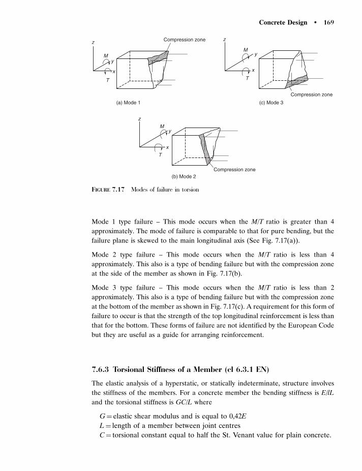
Mode 1 type failure – This mode occurs when the M/T ratio is greater than 4
approximately. The mode of failure is comparable to that for pure bending, but the
failure plane is skewed to the main longitudinal axis (See Fig. 7.17(a)).
Mode 2 type failure – This mode occurs when the M/T ratio is less than 4
approximately. This also is a type of bending failure but with the compression zone
at the side of the member as shown in Fig. 7.17(b).
Mode 3 type failure – This mode occurs when the M/T ratio is less than 2
approximately. This also is a type of bending failure but with the compression zone
at the bottom of the member as shown in Fig. 7.17(c). A requirement for this form of
failure to occur is that the strength of the top longitudinal reinforcement is less than
that for the bottom. These forms of failure are not identified by the European Code
but they are useful as a guide for arranging reinforcement.
7.6.3 Torsional Stiffness of a Member (cl 6.3.1 EN)
The elastic analysis of a hyperstatic, or statically indeterminate, structure involves
the stiffness of the members. For a concrete member the bending stiffness is E/lL
and the torsional stiffness is GC/L where
G¼ elastic shear modulus and is equal to 0,42E
L¼ length of a member between joint centres
C¼ torsional constant equal to half the St. Venant value for plain concrete.
Compression zone
Compression zone
Compression zone
(a) Mode 1
(b) Mode 2
(c) Mode 3
z
My
x
T
z
My
x
T
z
My
x
T
FIGURE 7.17 Modes of failure in torsion
Concrete Design � 169

The torsional constant C for a rectangular reinforced concrete section
C ¼ 0,5�h3minhmax
The factor of 0,5 incorporated in the value of C makes allowance for warping by
halving the polar second moment of area of the section.
The value of the St. Venant factor � is obtained from the following table:
The St. Venant torsional stiffness of a non-rectangular section may be obtained by
dividing the section into a series of rectangles and summing the torsional stiffness of
these rectangles (cl 6.3.1(5), EN). The division of the rectangles is arranged to
maximize the calculated stiffness. This will be generally achieved if the widest
rectangle is made as long as possible.
EXAMPLE 7.11 Torsional stiffness of a member. Determine the torsional stiffness
of a member with a rectangular cross section 150� 300 mm, length between joint
centres 4 m. Assume Grade C25/30 concrete.
Static modulus of elasticity of concrete (Table 3.1, EN)
Ecm ¼ 22½ð fcm þ 8Þ=10Þ0,3¼ 22½ð25 þ 8Þ=10�0,3
¼ 31,5 GPa:
Shear modulus
G ¼ 0,42Ecm ¼ 0,42 � 31,5 ¼ 13,2 GPa:
Torstional constant, �¼ 0,23 from Table 7.1
C ¼ 0,5�h3minhmax ¼ 0,5 � 0,23 � 1503 � 300 ¼ 116,4E6 mm4
Torstional stiffness of the member
GC=L ¼ 13,2 � 116,4E6=ð4E3 � 1E3Þ ¼ 384 kNm:
7.6.4 Equivalent Thin Walled Section (cl 6.3.1(3), EN)
In practice, there are solid and hollow sections which are reinforced to resist bending
and torsion. Experiments (Hsu, 1968 and Lampert, 1971) show that the core area
does not contribute significantly to the torsional resistance. For design purposes
TABLE 7.1 St. Venant torsional factors for plain concrete.
hmax/hmin 1 1,5 2 3 5 45
� 0,14 0,20 0,23 0,26 0,29 0,33
170 � Chapter 7 / Shear and Torsion

solid sections are replaced by thin walled sections (Fig. 7.18) where, for a rectangular
section, the effective wall thickness
tef,i ¼ total area/outer circumference
¼ A=u ¼ b h= ½2ðbþ hÞ�5 actual wall thickness: ð7:17Þ
The wall thickness should be at least twice the cover to the longitudinal
reinforcement plus the bar size.
Area enclosed by the centre lines of the connecting walls including the inner
hollow areas
Ak ¼ ðb� tÞðh� tÞ ð7:18Þ
7.6.5 Torsion Reinforcement (cl 9.2.3, EN)
Plain concrete is able to resist a small torsional moment, but because in practice
the concrete may crack the section is always reinforced. The torsional reinforcement
is generally in the form of closed links (Fig. 9.6, EN) similar in shape and additional
to those required for shear reinforcement.
The truss analogy, used to develop theory for shear resistance, can also be used for
torsional resistance. If each wall of a rectangular hollow section is considered as
shown in Fig. 7.4, then Eq. (7.3) can be modified to form an equation to express the
torsional resistance of the shear reinforcement about the longitudinal axis
TRd2 ¼ 2Fsw sin �Ak ¼ 2AswfywdðAC=sÞ sin �Ak
¼ 2Aswfywdðcot � þ cot�Þ sin �Ak ð7:19Þ
where Ak is the area enclosed by the centre lines of the connecting walls.
b
h
A = shaded areau = circumference of A
Ak = shaded area = (b−t )(h−t )uk = circumference of Ak = 2(b−t )(h−t )
tThickness = A/u= bh/[2(b+h)]
FIGURE 7.18 Equivalent thin walled section
Concrete Design � 171
For vertical links �¼ 908 and assuming �¼ 458 then this equation is equivalent to
Eq. 6.28, EN.
Similarly the torsional resistance of the concrete about the longitudinal axis
TRd1 ¼ 2Fcn sin �Ak ¼ 2tðAC sin �Þfcrushing sin �Ak
¼ 2tAknfcdðcot � þ cot �Þ sin2 � ð7:20Þ
For vertical stirrups �¼ 908 then this is comparable with Eq. 6.30, EN.
Equating total axial forces at section 2-2 (Fig. 7.4), where Asl is the total area of
axial steel to resist torsion
4Fc cos � ¼ Asl fyld ðiÞ
Resolving forces vertically at B
Fc sin � ¼ AswfywdðAC=sÞ sin � ðiiÞ
Equating values of Fc from Eqs (i) and (ii)
Fc ¼ Asl fyld= cos � ¼ ukðAsw=sÞfywdACsin�= sin �
Asl fyld ¼ uk cos �ðAsw=sÞfywdðcot � þ cot �Þ sin �= sin �
¼ uk cos �½TRd2=ð2Ak cot �Þ�ðcot � þ cot �Þ sin �= sin � ðiiiÞ
Asl fyld ¼ uk cot �½TRd2=ð2AkÞ� ð7:21Þ
From Eq. (iii) a relationship for tan� may be obtained
Asl fyld ¼ ukðAsw=sÞfywd cot2 �
tan2 � ¼ ukðAsv fywd=sÞ=ðAsl fyldÞ ð7:22Þ
Combining Eqs (7.21) and (7.22)
TRd2 ¼ 2Ak½ðAsvfywd=sÞðAsl fyld=ukÞ�0,5
ð7:23Þ
Recommended values of cot� vary between 1 and 2,5 (cl 6.3.2(2), EN) the same
range as for shear resistance. When considering combined actions, the angle � is the
same for torsion and shear design. Notice that than � is related to the ratio of links
to the longitudinal steel (Eq. 7.22).
7.6.6 Arrangement of Torsion Reinforcement(cl 9.2.3, EN)
Careful detailing of the torsion reinforcement is required if it is to be effective. To
intercept the diagonal cracks in the concrete the spacing of the links (s) is similar to
that for shear resistance.
The longitudinal torsional reinforcement must be distributed evenly round the
inside perimeter of the links to prevent a mode 3 type failure as shown in Fig. 7.17(c).
172 � Chapter 7 / Shear and Torsion

The distance between bars should not exceed 350 mm (cl 9.2.3(4), EN) and at least
four bars, one in each corner should be used.
The torsion reinforcement should extend a distance equal to the largest dimension
of the section beyond where it theoretically ceases to be required. This requirement
is because of additional axial stresses introduced due to torsion, cracks spiralling
for considerable lengths along a member, and to avoid abrupt changes of rein-
forcement.
EXAMPLE 7.12 Torsion reinforcement. A rectangular section of a beam is subject
to a design torsional moment TEd¼ 50 kNm (Fig. 7.19). The cross section is 600 mm
deep and 300 mm wide and made from C25/30 concrete. Determine the torsion
reinforcement required. Assume that the section has been designed for bending and
that the area of tensile reinforcement required from bending calculations is
Asl¼ 1200 mm2.
Equivalent wall thickness of the section (Fig. 7.18) from Eq. (7.17)
t ¼ bh=½2ðbþ hÞ� ¼ 300 � 600=½2ð300 þ 600Þ� ¼ 100 mm:
Area enclosed by the centre lines of enclosing walls
Ak ¼ ðb� tÞðh� tÞ ¼ ð300 � 100Þð600 � 100Þ ¼ 100E3 mm2
uk ¼ 2½ðb� tÞ þ ðh� tÞ� ¼ 2½ð300 � 100Þ þ ð600 � 100Þ� ¼ 1400 mm:
Shear stress in the longer wall of the section from torsion (Eq. 6.26, EN)
�t,itef,i ¼ TEd=ð2AkÞ ¼ 50E6=ð2 � 100E3Þ ¼ 250 MPa:
Shear force in the longer wall of the section (Eq. 6.27, EN)
VEd,i ¼ �t,itef,izi ¼ 250 � ð600 � 2 � 30Þ=1E3 ¼ 135 kN
Asw=s ¼ VEd,i=ðz fywdÞ ¼ 135E3=ð0,9 � 550 � 0,8 � 500Þ ¼ 0,682 mm:
Longitudinal spacing of T10 vertical links
sl ¼ 79=0,682 ¼ 115,8 mm, use sl ¼ 100 mm:
300
2T16
2 T16
T10-100
600
4T25 FIGURE 7.19 Example: torsion reinforcement
Concrete Design � 173

Maximum torsional moment of resistance (�¼ 458) (Eq. 6.30, EN)
TRd, max ¼ 2n�c fcdAktef,i sin � cos �
¼ ð2 � 0,54 � 25=1,5 � 100E3 � 100 � 0,707 � 0,707Þ=1E6
¼ 904TEdð50Þ kNm, satisfactory:
Strength reduction factor for concrete (Eq. 6.6, EN)
n ¼ 0,6ð1 � fck=250Þ ¼ 0,6ð1 � 25=250Þ ¼ 0,54:
Area of the longitudinal reinforcement (Eq. 6.28, EN)
�Asl ¼ TEd cot � uk=ð2AK fydÞ
¼ 50E6 � 1 � 1400=ð2 � 100E3 � 500=1,15Þ ¼ 805 mm2
Use 6 longitudinal bars. Two of these bars can be combined with the tension
reinforcement (cl 6.3.2(3), EN)
Asl¼ 1200þ 805/3¼ 1468 mm2. Tension reinforcement 4T25 (1964 mm2).
Area of other four bars¼ 2/3� 805¼ 537 mm2. Use 4T16¼ 804 mm2.
Maximum longitudinal spacing of links (Eq. 9.6, EN)
sl,max ¼ 0,75dð1 þ cot�Þ ¼ 0,75 � 540 � ð1 þ 0Þ ¼ 4054 slð100Þ mm:
Also (cl 9.2.3, EN)
sl, max ¼ u=8 ¼ 2ðbþ dÞ=8 ¼ 2 � ð300 þ 600Þ=8 ¼ 2255 bð300Þ mm, use
sl ¼ 100 mm:
Shear reinforcement ratio (Eq. 9.4, EN)
w ¼ Asv=ðs bw sin �Þ ¼ 2 � 79=ð100 � 300 � 1Þ ¼ 0,00527:
Minimum shear reinforcement ratio (Eq. 9.5, EN)
min ¼ 0,08f 0,5ck =fyk ¼ 0,08 � 250,5=500 ¼ 0,00085 wð0,00527Þ, acceptable:
REFERENCES AND FURTHER READING
ASCE-ACI Committee 445 (1998) Recent approaches to shear design of structural concrete,
Jnl Struct Eng 124, No 12, Dec, 1373–1417.
ASCE-ACI Committee 426 (1973) The shear strength of reinforced concrete structures, Proc.
ASCE, 99, NO ST6, 1091–1187.
174 � Chapter 7 / Shear and Torsion
Baumann, T. and Rusch, H. (1970) Tests studying the dowel action to the flexural tensile
reinforcement of reinforced concrete beams, Berlin, William Ernst und Sohn. Deutscher
Ausschuss fur Stahlbeton, Heft 210, 42–82.
Chana, P.S. (July 1981) Some aspects of modelling the behaviour of reinforced concrete under
shear loading, Cement and Concrete Association, Technical Report 543, 22.
Evans, R.H. and Kong, F.K. (1967) Shear design and British Code CP 114. Structural Engineer,
45(4), 153–187.
Hsu, T.T.C. (1968) Torsion of structural concrete - behaviour of reinforced rectangular members.
Special Publication, No 18-10, ACI, 261–306.
Kong, F.K. (1978) Bending, Shear and Torsion, Chapter 1, Developments in Prestressed Concrete.
Applied Science, London, Vol. 1, 1–68.
Lampert, P. (1971) Torsion and bending in reinforced and prestressed concrete beams. Proc. ICE,
Dec, Vol. 50, 487–505.
Lessig, N.N. (1959) The determination of the load bearing capacity of rectangular reinforced
concrete sections subject to combined torsion and bending. Study No 5, Concrete and Reinforced
Concrete Inst., Moscow, 5–28.
Loov, R.E. and Patnaik, A.K. (1994) Horizontal shear strength of composite concrete beams with a
rough interface. PCIJ, 39(1), 48–109.
Placas, A. and Regan, P.E. (1971) Shear failure of reinforced concrete beams. Proc. ACIJ. October,
763–773.
Reynolds, G.C., Clark, J.L. and Taylor, H.P.J. (1974) Shear provisions for prestressed concrete in
the unified code CP 110(1972). Technical Report 42.500, Cement and Concrete Association,
London, 16.
Regan, P.E. (2004) Punching of slabs under highly concentrated loads. Proc. ICE, Struct. and Bu.,
157, April, 165–171.
Ritter, W. (1899) Die bauweiser hennebique. Schweizerische Bauzeitung, 33(7), 59–61.
Saemann, J.C. and Washa, G.W. (1964) Horizontal shear connections between precast beams and
cast-in-place slabs. Proc. ACI, V61, 11, Nov, 1383–1408.
Shioya, T., Iguro, M., Nojiri, Y., Akiayma, H. and Okada, T. (1989) Shear strength of large concrete
beams, fracture mechanics: application to concrete. SP-118, ACI, Detroit, 259–279.
Taylor, H.P.J. (1974) The fundamental behaviour of reinforced concrete beams in bending
and shear. Proc. ACI - ASCE Shear Symposium, Ottawa, ACI Publication SP 42, ACIJ,
Detroit, 43–77.
Walraven, J.C., Vos, E. and Reinhardt, H.W. (1978) Experiments on shear and transfer in cracks in
concrete, Pt 1, description of results. Report 5-79-3, Stevin Laboratory, Delft University of
Technology, The Netherlands, 84.
Walsh, P.E., Collins, M.P., Archer, F.E. and Hall, A.S. (1966) The ultimate strength design of
rectangular reinforced concrete beams subjected to combined torsion, bending and shear.
Trans. ICE, Australia, 143–157.
Yoon Y.S., Cook W.D. and Mitchell D. (1996). Minimum shear reinforcement in normal, medium
and high strength concrete beams. ACIJ, 93(5), 576–584.
Concrete Design � 175
C h a p t e r 8 / Anchorage, Curtailment andMember Connections
8.1 ANCHORAGE (cl 8.4, EN)8.1.1 Introduction
Reinforcing bars are produced in stock lengths, e.g. approximately 6 m for 8 mm
diameter, and 12 m for 32 mm diameter. These stock lengths may be cut or
terminated for the following reasons:
(a) to fit the member,
(b) to economise in steel, e.g. curtailment of bars in order to use fewer bars where
the bending moment reduces along the length of a member and
(c) to make construction easier.
A bar may be terminated as straight, hook, bend or loop (Fig. 8.1, EN). Equivalent
anchorage lengths for design purposes are shown (Fig. 8.1).
A reinforcing bar must be adequately anchored to prevent withdrawal from the
concrete before it has reached its full tensile strength. The greater the angle change
at the end of the bar the more effective the anchorage, but this is offset by the
greater cost for shaping. Some situations in practice that require calculations for
bond length (shown as a heavy black line) are shown in Fig. 8.2.
8.1.2 Anchorage of Bars (cl 8.4, EN)
The withdrawal of straight bar, with adequate cover and embedded in concrete, is
prevented by the bond shear stresses parallel to the surface of the bar and the
concrete. Bond is due to the combined effects of adhesion, friction and, in the case of
deformed bars, the bearing of the projecting ribs. Plain bars withdraw from the
concrete, but ribbed bars introduce radial tensile stresses in the concrete which
generally produce splitting and cracking of the concrete.
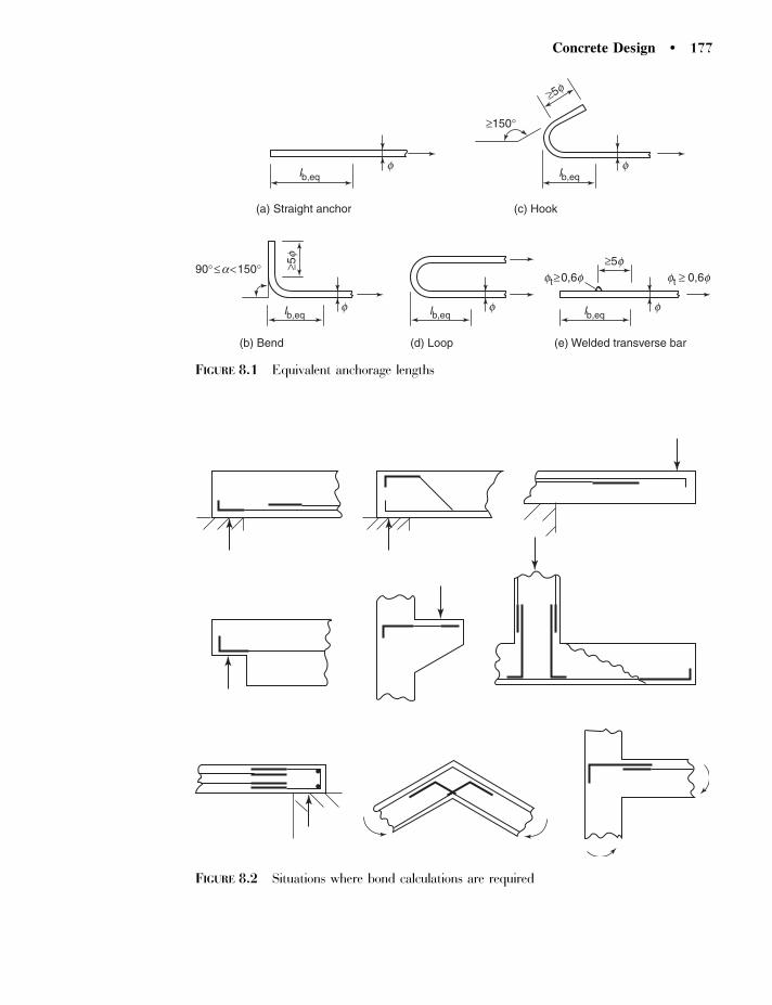
f f
f f f
lb,eq lb,eq
lb,eq lb,eq lb,eq
≥150°
90°≤a<150°ft≥0,6f ft ≥ 0,6f
≥5f
≥5f ≥5f
(a) Straight anchor
(b) Bend (d) Loop (e) Welded transverse bar
(c) Hook
FIGURE 8.1 Equivalent anchorage lengths
FIGURE 8.2 Situations where bond calculations are required
Concrete Design � 177

The factors that affect the bond are:
(a) concrete strength,
(b) axial stress in the bar,
(c) surface condition of the bar,
(d) straight or hooked bar,
(e) welding as anchorage,
(f) transverse reinforcement,
(g) pressure transverse to the bar,
(h) tension or compression in the bar and
(i) dowel forces at right angles to the reinforcement.
All these factors, except (i), are allowed for in Table 8.2, EN.
When a steel bar is pulled out of concrete bond stresses arise due to the differences
in the axial stresses in the steel bar. This results in varying bond stresses along the
length of the bar.
If for simplicity, the ultimate bond shear stresses are assumed to be uni-
formly distributed as shown in Fig. 8.3, then from the equilibrium of forces,
tensile force in bar¼ bond shear force
�2=4sd ¼ �lb fbd
Rearranging, the basic anchorage length (Eq. 8.3, EN)
lb,req ¼ ð�=4Þðsd=fbdÞ:
The design axial stress in the bar (sd) is at the position from where anchorage
is measured. The design bond stress (fbd) between the steel and the concrete
varies with the surface condition of the bar and tensile strength of the concrete
(Eq. 8.2, EN).
fbd ¼ 2,25n1n2fctd
n1 is related to bond position of the bar, n2 is related to bar diameter and the tensile
strength of the concrete (cl 8.4.2(2), EN)
fctd ¼ �ct fctk0,05=�c
Bond shear stresses
Bond length lb Steel bar
Diameter f
Tensile force
Concrete FIGURE 8.3 Anchorage of a straight bar
178 � Chapter 8 / Anchorage, Curtailment and Member Connections

The 5 per cent fractile tensile strengths of concrete ( fctk0,05) are obtained from
Table 3.1, EN (Annex A2).
Ribbed bars are more difficult to withdraw from concrete because their surfaces are
rougher (Fig. 8.4). At bond failure, a ribbed bar splits and cracks the surrounding
concrete producing a volume change in the concrete (Reynolds, 1982). Despite the
different failure mechanisms the ultimate bond strength is also related to the tensile
strength of the concrete, although as expected, the values are greater than for plain
bars.
Welded mesh reinforcement is difficult to withdraw from concrete because of the
strength of the weld(Fwd) to the transverse reinforcement (Eq. 8.9, EN).
Fbtd ¼ Fwd � 16As fcd�t=�l
The basic anchorage length (lb,req) is factored (Table 8.2, EN), to allow for practical
conditions e.g. hooks, concrete cover and confinement. The design anchorage length
(Eq. 8.4, EN)
lbd ¼ �1�2�3�4lb,req � lb, min
Where there is insufficient length available for anchorage of a straight bar then
bends, hooks or loops are used as shown in Fig. 8.1. To prevent overstraining and
cracking of the bar the radii of the bends should not be too small. This is controlled
by the mandrel diameter (Table 8.1, EN). For �� 16 mm the mandrel diameter
is 4�. For �4 16 mm the mandrel diameter is 7�.
In practice, the use of bends and hooks is kept to a minimum because of the cost
involved in their formation. Although improved bond characteristics of straight bars
has reduced the use of bends and hooks they are required where bond length is
restricted, e.g. supports for beams, starter bars in bases, links, bent-up shear
reinforcement and member connections.
8.2 BAR SPLICES
8.2.1 Introduction (cl 8.7, EN)
In reinforced concrete construction splices between the ends of bars are required to
extend their length or to facilitate construction. Splices transferring stress are
generally lapped, but may also be welded or joined with mechanical devices
(Paterson and Ravenshill, 1981). Splices should be placed, wherever possible, away
from points of high stress and preferably should be staggered. Laps in fabric may be
FIGURE 8.4 Deformed bar
Concrete Design � 179

layered or nested to maintain the lapped bars in one plane. Good detailing should
avoid spalling of the concrete in the neighbourhood of the splice and the width of the
cracks should not exceed allowable values. Various types of splices are shown in
Fig. 8.5.
8.2.2 Lap Splices (cl 8.7.2, EN)
The simplest, cheapest and most common type of splice is lapped as shown in
Fig. 8.5(a). The force in one bar is transferred to the other by bond between the steel
and the concrete. The design lap length (Eq. 8.10, EN),
lo ¼ �1�2�3�4�5�6lb,req � lo, min
The efficiency of splices depends on adequate cover and resistance to bursting of the
concrete for deformed bars. Where cover is inadequate the situation is improved by
transverse reinforcement, e.g. stirrups, which enclose the longitudinal reinforcement
and increase the tensile bursting strength of the concrete.
8.2.3 Mechanical Splices (cl 8.7.1, EN)
The suitability of the coupling sleeve shown in Fig. 8.5(b) should be demonstrated.
The sleeve is not in common use but is suitable for bars in compression provided that
the sawn square cut ends are held in concentric contact. The sleeves advantage is
that it saves on length of steel and reduces congestion of the bars. The disadvantages
are increased cost and reduction of concrete cover. This type of sleeve may be used
for bars in tension provided that it is demonstrated to be suitable.
8.2.4 Welded Splices (cls 3.2.5, 8.7.1, EN)
Welded splices are not often used on site because of the disadvantages of cost and
supervision required. Welding is capable of producing a full strength connection and
practical recommendations are:
(1) reinforcing steel must be suitable for welding (Pr EN 10080),
(2) welded joints should not occur at or near bends,
Lap length
(a) Lapped splice
(c) Butt weld
(b) Mechanical connection (or coupler)
(d) Lap welded diameter f
FIGURE 8.5 Bar splices
180 � Chapter 8 / Anchorage, Curtailment and Member Connections

(3) where possible, joints in parallel bars of the principal tensile reinforcement
should be staggered in the longitudinal direction,
(4) butt welded joints in compression resist 100 per cent of the design strength, but
joints in tension should be designed to resist 80 per cent of the design strength.
Fillet welded lap connections, as shown in Fig. 8.5(d), are used where prefabricated
cages of reinforcement, or mesh, are placed in a shutter and welded together in
place. Alternatively, they may be used for the steel connections for precast
reinforced concrete elements. The length and spacing of welds should be sufficient
to transmit the design load in the bar (cl 8.6. EN).
8.3 CURTAILMENT OF REINFORCING BARS
8.3.1 Introduction
Curtailment of reinforcing bars is the stopping of some of the reinforcing bars in
tension, or compression, where they are no longer needed for strength purposes.
Curtailment can be applied to simply supported beams but it is generally not
economic and the real advantages occur with repetitive multi-span beams and slabs.
It can also be used to facilitate construction by curtailing bars to practical lengths
which are easier to handle. However, the saving in steel is off-set by increased design
calculations, detailing and site supervision.
8.3.2 Theoretical Curtailment
A part of a beam subject to a bending moment, which varies along is length, is shown
in Fig. 8.6.
Bending moment diagram
0,5 M(approx.)
M
B
B
A
ATheoreticalcurtailment point
Practicalcurtailment point FIGURE 8.6 Theoretical curtailment
Concrete Design � 181
At section A, the bending moment is a maximum and four bars are required in
tension. Further along the beam at section B, the bending moment has reduced to
approximately half and only two bars are required. The bars are shown in Fig. 8.6 at
different levels in the elevation for purposes of illustration. Theoretically two bars
can be stopped, or curtailed, at this section. However, the bars must be anchored by
further extension. The shear force at this section also introduces an axial stress in the
bars and this must be taken into account (cl 6.2.3(7), EN).
8.3.3 Practical Curtailment (cl 9.2.1.3, EN)
A bar extends beyond the point at which it is theoretically no longer required for the
following reasons:
(a) Continuing bars are at the design strength.
(b) Large cracks may appear at the curtailment section because of the abrupt
change in section properties. This may reduce the shear strength of the member
and therefore it is advisable to stagger the curtailment points in heavily
reinforced members.
(c) To allow for inaccuracies in loading and theoretical analysis.
(d) To allow for inaccuracies in placing bars.
(e) To resist the shear force. The shear force at a section in bending introduces an
additional tensile force in the longitudinal steel. For singly reinforced beams this
is catered for by increasing the bond length by the effective depth (d) (cl 6.2.2,
EN). For beams with shear reinforcement (cl 9.2.1.3(2), EN), the additional
bond length is calculated from the additional tensile force in the longitudinal
reinforcement which is related to the shear force (cl 6.2.3(7), EN),
�Ftd ¼ 0,5VEdðcot � � cot�Þ
EXAMPLE 8.1 Curtailment of bars. Determine (a) the theoretical and (b) practical
curtailment point for 2T20 bars for the cantilever beam shown in Fig. 8.7. Assume
b¼ 300 mm, d¼ 700 mm, and C20/25 Grade concrete.
Stage (1) For a beam with shear reinforcement the theoretical curtailment point
occurs where the design bending moment plus shear force can be resisted by 2T20
reinforcing bars.
Equating moments of resistance at a distance x from the end of the cantilever
Mr ¼ MEd
Aszð fyd ��Ftd=AsÞ ¼ qx2=2
Aszð fyd � 0,5qx=AsÞ ¼ qx2=2
182 � Chapter 8 / Anchorage, Curtailment and Member Connections

Assuming that the steel stress is at the design strength, z¼ 0,9d¼ 630 mm, and
q¼ 20 kN/m¼ 20 N/mm, the value of
x ¼ �z=2 þ ð½z=2Þ2 þ 2As fydz=q�0,5
¼ �630=2 þ ½ð630=2Þ2 þ 2 � 628 � 500=1,15 � 630=20�0,5¼ 3,844E3 mm
The theoretical curtailment point for 2T20 bars in 3,84 m from the end of the
cantiliver.
Stage (2) Basic anchorage length (Eq. 8.3, EN)
lb,req ¼ ð�=4Þðsd=fbdÞ ¼ 20=4 � ð500=1,15Þ=2,25 ¼ 966 mm
where the design bond stress for high bond bars (Eq. 8.2, EN)
fbd ¼ 2,25n1n2 fctd ¼ 2,25 � 1 � 1 � 1,5=1,5 ¼ 2,25 MPa
Design bond length with 30 mm cover (Eq. 8.4, EN)
lbd ¼ �1�2�3�4�5�6lb,req ¼ 1 � 0,85 � 966 ¼ 821 mm
where
�2 ¼ 1 � 0,15 � ðcd � �Þ=� ¼ 1 � 0,15 � ð30 � 20Þ=20 ¼ 0,85:
Check if greater than the minimum anchor length in tension (cl 8.4.4, EN)
lb,min ¼ 0,3lb,req ¼ 0,3 � 966 ¼ 290; or 10� ¼ 10 � 20 ¼ 200; or 100 mm:
Stage (3) Distance of the practical curtailment point from the end of the
cantilever
x0 ¼ x� lbd ¼ 3,84 � 0,821 ¼ 3,02 m, Use x0 ¼ 3 m:
q=20kN/m
4T20 2T20 T8-240
d=700
5m
x ′=3m
FIGURE 8.7 Example: curtailmentof bars
Concrete Design � 183
8.4 MEMBER CONNECTIONS
8.4.1 Introduction
Connections and joints in a structure may be classified as follows:
(a) Construction joints introduced between concrete pours, sections or levels to
facilitate construction. These are particularly useful for in situ concrete work,
e.g. foundations can be concreted first and the columns later. In many cases,
these joints transmit forces but in other cases the requirements are that they
should resist fire, corrosion, and be durable and sound proof.
(b) Movement joints are required to allow free expansion and contraction to occur
in the structure due to temperature, shrinkage, creep, settlement, etc. and
prevent a build-up of stresses (Alexander and Lawson, 1981).
(c) Structural connections are required to transmit forces from one member to
another, or one part of a structure to another. It is these connections that
require calculations.
It is possible for a structural connection to be subject to any combination of axial
force, shear force and bending moment in relation to three perpendicular axes.
Generally in design the situation is simplified to forces in one plane. The distribution
of forces within the connection is generally complex and complete knowledge and
understanding is not available. In practice, simple conservative assumptions are
made in calculations as shown in the following examples.
The forces acting on a structural connection must be consistent with the structural
analysis of the whole structure. Connections are assumed to be either ‘rigid’, or
‘pinned’, or ‘on rollers’. In reality, such connections do not exist but some assumptions
must be made when analysing the complete structure. The analysis produces
moments and forces and the members and connections can then be designed.
8.4.2 Simple Beam Supports (cl 9.2.1.4, EN)
Beams which are described as simply supported are assumed in structural analysis to
be pin-ended. For real structures, the reaction is distributed on the bearing and there
is a frictional force acting between the bearing surfaces.
At the supports of simply supported beams there are special requirements to ensure
that the reinforcing bars are anchored (Fig. 9.3, EN). The bearing area and bearing
stresses also require detailed consideration. In general, the length of bearing in line
with the span (a1) should not be less than recommended minimum values (Table
10.2, EN) which range from 25 to 140 mm.
EXAMPLE 8.2 Direct beam support. Determine the bearing length for a simply
supported floor beam shown in Fig. 8.8. Design forces at the support VEd¼ 250 kN
184 � Chapter 8 / Anchorage, Curtailment and Member Connections
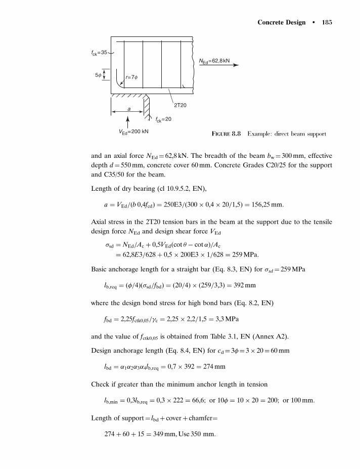
and an axial force NEd ¼ 62,8 kN. The breadth of the beam bw¼ 300 mm, effective
depth d¼ 550 mm, concrete cover 60 mm. Concrete Grades C20/25 for the support
and C35/50 for the beam.
Length of dry bearing (cl 10.9.5.2, EN),
a ¼ VEd=ðb 0,4fcdÞ ¼ 250E3=ð300 � 0,4 � 20=1,5Þ ¼ 156,25 mm:
Axial stress in the 2T20 tension bars in the beam at the support due to the tensile
design force NEd and design shear force VEd
sd ¼ NEd=Ac þ 0,5VEdðcot � � cot �Þ=Ac
¼ 62,8E3=628 þ 0,5 � 200E3 � 1=628 ¼ 259 MPa:
Basic anchorage length for a straight bar (Eq. 8.3, EN) for sd¼ 259 MPa
lb,req ¼ ð�=4Þðsd=fbdÞ ¼ ð20=4Þ � ð259=3,3Þ ¼ 392 mm
where the design bond stress for high bond bars (Eq. 8.2, EN)
fbd ¼ 2,25fctk0,05=�c ¼ 2,25 � 2,2=1,5 ¼ 3,3 MPa
and the value of fctk0,05 is obtained from Table 3.1, EN (Annex A2).
Design anchorage length (Eq. 8.4, EN) for cd¼ 3�¼ 3� 20¼ 60 mm
lbd ¼ �1�2�3�4lb,req ¼ 0,7 � 392 ¼ 274 mm
Check if greater than the minimum anchor length in tension
lb,min ¼ 0,3lb,req ¼ 0,3 � 222 ¼ 66,6; or 10� ¼ 10 � 20 ¼ 200; or 100 mm:
Length of support¼ lbd þ coverþ chamfer¼
274 þ 60 þ 15 ¼ 349 mm, Use 350 mm:
NEd=62,8kN
VEd=200 kN
2T20
r=7f5f
a
fck=35
fck=20
FIGURE 8.8 Example: direct beam support
Concrete Design � 185

Minimum length of bearing (Table 10.2, EN) for Ed/fcd¼ 0,4 for a floor, where
a1,min¼ 305 350 mm therefore satisfactory.
8.4.3 Beam-to-Beam Connections
Secondary beams of the same, or different, depths intersect main beams at right
angles as shown in Fig. 8.9. This connection is assumed to be a ‘rigid’ connection in
the structural analysis and therefore is designed to resist a bending moment, a shear
force and sometimes an axial force.
Where secondary beams intersect the main beam from both sides the practical
arrangement of steel is shown in Fig. 8.9. The lap lengths are the full design lengths.
Alternative arrangements are shown in Figs 9.1 and 9.4, EN. Where only one
secondary beam intersects the main beam the steel arrangement and design is more
complicated (Fig. 8.10).
Lap Lap
FIGURE 8.9 Beam-to-beam connection
M1=50kNm
150kNm
Main beam B
Solution (a)
Solution (b)
600
400
q=25kN/m at ultimate load
3T16 3T16
3T16
4T20
4T20 Secondarybeam A4 m
250350
400
1,51m 0,58m
+
−
CL
I
Note: links not shown
FIGURE 8.10 Example: beam-to-beam connection
186 � Chapter 8 / Anchorage, Curtailment and Member Connections
Similar arrangements can be used for the intersection of slabs and beams, except
that the loop bars in the design example are arranged horizontally because of the
reduced depth of slab.
EXAMPLE 8.3 Beam-to-beam connection. Design the connection between the
secondary beam A and the main beam B shown in Fig. 8.10. The loading and
bending moment diagram are shown above the diagram. Assume C30/35 Grade
concrete.
Solution (a) (Fig. 8.10a)
Area of bars required to resist the hogging bending moment and shear force at
point 1
As ¼ M=ð fydzÞ þ�Ftd=fyd ¼ ð1=fydÞðM=zþ 0,5VEdÞ
¼ ð1,15=500Þ½50E6=ð0,9 � 350Þ þ 0,5 � 100E3� ¼ 480 mm2:
Use 3T16 (603 mm2), and extended into the top of the beam with a 908 bend.
Area of steel (603 mm2) is greater than the minimum (480 mm2) therefore the
reduced axial steel stress
sd ¼ 480=603 � 500=1,15 ¼ 346 MPa:
Basic anchorage length (Eq. 8.3, EN)
lb,req ¼ ð�=4Þðsd=fbdÞ ¼ 16=4 � 346=3 ¼ 461 mm
where the design bond stress for high bond bars (Eq. 8.2, EN)
fbd ¼ 2,25 fctk0,05=�c ¼ 2,25 � 2=1,5 ¼ 3 MPa:
Design anchorage length (Eq. 8.4, EN) if cover cd¼ 50 mm
lbd ¼ �1�2�3�40,7lb,req ¼ 0,7 � 461 ¼ 323 mm
Design anchorage lengthþ cover¼ 323þ 50¼ 3735 b (400) mm, acceptable.
Solution (b) (Fig 8.10 (b))
The essence of this variation is the insertion of 3T16 mm loop bars at the end of
beam A as shown in Fig. 8.10(b).
Theoretical curtailment point of the 16 mm bars in the bottom of the secondary
beam A at a distance x from the inside face of the main beam B.
Moments of resistance in kNm (z¼ 0,9� 350¼ 315 mm),
Mr ¼ Aszð fyd ��Ftd=AsÞ ¼ Aszð fyd � 0,5VEd=AsÞ
¼ Asz½ fyd � 0,5=AsðV � qxÞ� ¼ Aszfyd � 0,5zðV � qxÞ�
¼ ½603 � 315 � 500=1,15 � 0,5 � 315 � 100 þ 0,5 � 315 � 25x�=1E6 ðiÞ
Concrete Design � 187

MEd ¼ R1x�M1 � wx2=2 ¼ 100x� 50 � 25x2=2 ðiiÞ
Equating (i) and (ii)
x2 � 7,685xþ 9,34 ¼ 0; hence x ¼ 1,51 m:
Basic required lap length for a fully stressed 16 mm diameter bar
lb,req ¼ ð�=4Þðsd=fbdÞ ¼ 16=4 � ð500=1,15Þ=3 ¼ 580 mm
where the design bond stress for high bond bars (Eq. 8.2, EN)
fbd ¼ 2,25fctk0,05=�c ¼ 2,25 � 2=1,5 ¼ 3 MPa:
Design lap length (Eq. 8.10, EN) assuming more than 30 per cent lapped in tension
lo ¼ �1�2�3�4�5�6lb,req � 1 � lb,req ¼ 580 mm
which is greater than (Eq. 8.11, EN)
lo, min4ð0,3�6lb,req; 15�; 200 mmÞ
¼ ð0,3 � 580; 15 � 16; 200Þ ¼ ð174; 240; 200Þmm:
The arrangement of reinforcement is shown in Fig. 8.10(b).
8.4.4 Beam-to-Column Connections
Beams and columns, of the same or different widths, intersect at right angles as
shown in Fig. 8.11. These connections are assumed to be ‘rigid’ in the theoretical
structural analysis and therefore are designed to resist a combination of bending
moment, shear force and axial force. The connections are most efficient when the
intersecting members contain approximately 1 per cent reinforcement.
The two member connection shown in Fig. 8.11(a) occurs at the top of frame and
may be subject to moments which open or close the connection. Loops are an
adequate form of reinforcement when the moments are closing the joint, and
additional diagonal reinforcement is required for opening moments arranged as
shown.
The three member connection (Fig. 8.11(b)) may be reinforced with bends or with
loops (Fig. 8.11(c)). Experiments (Taylor, 1974) have shown that the closing corner
(Fig. 8.11(b)) is stronger than an opening corner.
The four member connection (Fig. 8.11(d)) is straightforward and reinforced with
straight bars lapped at construction joints.
188 � Chapter 8 / Anchorage, Curtailment and Member Connections
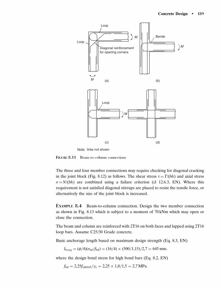
The three and four member connections may require checking for diagonal cracking
in the joint block (Fig. 8.12) as follows. The shear stress �¼T/(bh) and axial stress
¼N/(bh) are combined using a failure criterion (cl 12.6.3, EN). Where this
requirement is not satisfied diagonal stirrups are placed to resist the tensile force, or
alternatively the size of the joint block is increased.
EXAMPLE 8.4 Beam-to-column connection. Design the two member connection
as shown in Fig. 8.13 which is subject to a moment of 70 kNm which may open or
close the connection.
The beam and column are reinforced with 2T16 on both faces and lapped using 2T16
loop bars. Assume C25/30 Grade concrete.
Basic anchorage length based on maximum design strength (Eq. 8.3, EN)
lb,req ¼ ð�=4Þðsd=fbdÞ ¼ ð16=4Þ � ð500=1,15Þ=2,7 ¼ 645 mm:
where the design bond stress for high bond bars (Eq. 8.2, EN)
fbd ¼ 2,25fctk0,05=�c ¼ 2,25 � 1,8=1,5 ¼ 2,7 MPa:
Loop
Loop
Loop
BendsM
M
M
M
(a) (b)
(c) (d)
Diagonal reinforcementfor opening corners
Note: links not shown
FIGURE 8.11 Beam-to-column connections
Concrete Design � 189
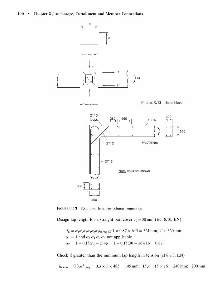
Design lap length for a straight bar, cover cd¼ 30 mm (Eq. 8.10, EN)
lo ¼ �1�2�3�4�5�6lb,req � 1 � 0,87 � 645 ¼ 561 mm, Use 560 mm:
�1 ¼ 1 and �3,�4,�5,�6 not applicable
�2 ¼ 1 � 0,15ðcd � �Þ=� ¼ 1 � 0,15ð30 � 16Þ=16 ¼ 0,87:
Check if greater than the minimum lap length in tension (cl 8.7.3, EN)
lb, min ¼ 0,3�6lb,req ¼ 0,3 � 1 � 483 ¼ 145 mm; 15� ¼ 15 � 16 ¼ 240 mm; 200 mm:
h
b
T
C
M
s
t
t
FIGURE 8.12 Joint block
2T16loops 2T16
2T16
2T12
380 560 300
300
400
500
M=70kNm
Note: links not shown
FIGURE 8.13 Example: beam-to-column connection
190 � Chapter 8 / Anchorage, Curtailment and Member Connections

The moment opens the connection therefore use diagonal bars. Area approximately
50 per cent of the main steel. Use 2T12.
Basic anchorage length based on maximum design strength (Eq. 8.3, EN)
lb,req ¼ ð�=4Þðsd=fbdÞ ¼ ð12=4Þ � ð500=1,15Þ=2,7 ¼ 483 mm
where the design bond stress for high bond bars (Eq. 8.2, EN)
fbd ¼ 2,25fctk0,05=�c ¼ 2,25 � 1,8=1,5 ¼ 2,7 MPa:
Design lap length for a straight bar (Eq. 8.10, EN)
lo ¼ �1�2�3�4�5�6lb,req � 1 � 0,775 � 483 ¼ 374 mm, Use 380 mm
�1 ¼ �3 ¼ �4 ¼ �5 ¼ �6 ¼ 1
�2 ¼ 1 � 0,15 ðcd � �Þ=� ¼ 1 � 0,15ð30 � 12Þ=12 ¼ 0,775:
The column and beam should be checked for axial load and shear forces and links
added. The arrangement of reinforcement to resist the moment is shown in Fig. 8.13
but the links are omitted for clarity.
8.4.5 Column-to-Base Connections
Columns generally intersect a base at right angles as shown in Fig. 8.14. This
connection is assumed to be a ‘rigid’ connection in structural analysis and therefore
is designed to resist a bending moment, a shear force and axial force.
The thickness of the base is related to the bond length required for the starter bars,
or the shear resistance of the base. The starter bars are hooked behind the
longitudinal bars in the base to reduce the design bond length. If the base is large
and the thickness of the base has to be increased, consideration should be given to a
pedestal base (Fig. 8.14). The lapped bars start approximately 75 mm above the top
surface of the base to provide a construction joint and provide a ‘kicker’ to locate the
column shuttering.
Pedestal
Starter bars
Note: links incolumn notshown
FIGURE 8.14 Column-to-baseconnection
Concrete Design � 191
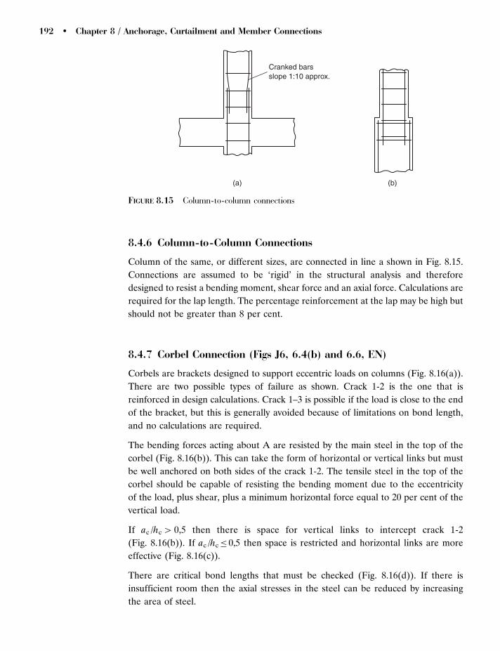
8.4.6 Column-to-Column Connections
Column of the same, or different sizes, are connected in line a shown in Fig. 8.15.
Connections are assumed to be ‘rigid’ in the structural analysis and therefore
designed to resist a bending moment, shear force and an axial force. Calculations are
required for the lap length. The percentage reinforcement at the lap may be high but
should not be greater than 8 per cent.
8.4.7 Corbel Connection (Figs J6, 6.4(b) and 6.6, EN)
Corbels are brackets designed to support eccentric loads on columns (Fig. 8.16(a)).
There are two possible types of failure as shown. Crack 1-2 is the one that is
reinforced in design calculations. Crack 1–3 is possible if the load is close to the end
of the bracket, but this is generally avoided because of limitations on bond length,
and no calculations are required.
The bending forces acting about A are resisted by the main steel in the top of the
corbel (Fig. 8.16(b)). This can take the form of horizontal or vertical links but must
be well anchored on both sides of the crack 1-2. The tensile steel in the top of the
corbel should be capable of resisting the bending moment due to the eccentricity
of the load, plus shear, plus a minimum horizontal force equal to 20 per cent of the
vertical load.
If ac /hc 4 0,5 then there is space for vertical links to intercept crack 1-2
(Fig. 8.16(b)). If ac /hc� 0,5 then space is restricted and horizontal links are more
effective (Fig. 8.16(c)).
There are critical bond lengths that must be checked (Fig. 8.16(d)). If there is
insufficient room then the axial stresses in the steel can be reduced by increasing
the area of steel.
Cranked barsslope 1:10 approx.
(a) (b)
FIGURE 8.15 Column-to-column connections
192 � Chapter 8 / Anchorage, Curtailment and Member Connections

Alternative shapes of corbels and arrangements of reinforcement are given in tests
(Somerville and Taylor, 1972).
The shear resistance is calculated as for a singly reinforced concrete cantilever with
an enhanced shear strength based on the effective depth/shear span ratio (cl 6.2.2(6),
EN). Shear reinforcement is added to resist all of the shear. Typical calculations are
shown in Example 7.10.
8.4.8 Half Joint (cl 10.9.4.6, EN)
This type of connection is useful when the construction depth is to be kept to a
minimum, e.g. a bean supported on cantilever beams in line. The general shape and
arrangement of reinforcement in a half joint is shown in Fig. 8.17.
The reinforcement is required to prevent the type of failure as shown in Fig. 8.17(a)
(Reynolds, 1969). The horizontal link, or loop, resists the moment and shear of VEd
Column
Corbel
ac
3
h c
2
1
Main steel to resistbending about A
Vertical linksto interceptcrack 1−2
Horizontal linksto interceptcrack 1−2
A
Column steel not shown
Critical bond lengths
(a) (b)
(c) (d)
ac/hc > 0,5
ac/hc < 0,5
FIGURE 8.16 Corbel connections
Concrete Design � 193

and the direct force HEd. The link must be securely anchored in the nib and beam.
The vertical end link resists the force VEd. The diagonal link also resists the moment
of forces about point A and duplicates the resistance of the horizontal and vertical
links. The prime function of the diagonal link is to strengthen an opening joint as in
beam to column connections.
EXAMPLE 8.5 Half joint. Design the connection as shown in Fig. 8.18(a). Assume
C25/30 concrete and design loads of VEd¼ 35 kN and HEd¼ 17,5 kN.
Tensile force in the horizontal link
Fs ¼ VEde=dþHEd þ 0,5VEd ¼ 35 � 165=250 þ 17,5 þ 0,5 � 35 ¼ 58,1 kN:
Area of steel required in a horizontal link to resist Fs
As ¼ Fs=fyd ¼ 58,1E3=ð500=1,15Þ ¼ 134 mm2
Use single horizontal link 2T12¼ 226 mm2
Reduced axial steel stress
sd ¼ 134=226 � 500=1,15 ¼ 258 MPa:
Basic anchorage length for the 12 mm link (Eq. 8.3, EN)
lb,req ¼ ð�=4Þðsd=fbdÞ ¼ ð12=4Þ � ð258=2,7Þ ¼ 287 mm
where the design bond stress for high bond bars (Eq. 8.2, EN)
fbd ¼ 2,25fctk0,05=�c ¼ 2,25 � 1,8=1,5 ¼ 2,7 MPa:
Design bond length of the horizontal link into the nib (Eq. 8.4, EN)
lbd ¼ �1�2�3�4lb,req ¼ 0,7 � 287 ¼ 201 mm:
Nib
A
B 45°
HEd = µ VEdVEd
ln
Diagonal link
End vertical link
Horizontal link
(a) (b)
FIGURE 8.17 Half-joint
194 � Chapter 8 / Anchorage, Curtailment and Member Connections

Minimum bond length in tension (cl 8.4.4, EN)
lb, min ¼ 0,3lb,req ¼ 0,3 � 287 ¼ 86 mm; 15� ¼ 15 � 12 ¼ 180 mm; 200 mm:
Bond length available for
nib ¼ eþ 210 � cover ¼ 165 þ 210 � 50 ¼ 3254lbdð201Þmm; acceptable:
Area of steel required in the end vertical single link to resist VEd
Asw ¼ VEd=ð fydÞ ¼ 35E3=ð500=1,15Þ ¼ 80,6 mm2
Use single end vertical T8 link Asw¼ 101 mm2
Area of steel required in a diagonal 458 link, ignoring the horizontal and vertical
links taking moments about A
Asw ¼ MA=ð fydzÞ ¼ 18,9E6=ð500=1,15 � 0,9 � 250 �ffiffiffi2
pÞ ¼ 137 mm2
Use single (2 legs) diagonal T10 link Asw¼ 157 mm2
Basic anchorage length for the 10 mm diagonal link (Eq. 8.3, EN)
lb,req ¼ ð�=4Þðsd=fbdÞ ¼ 10=4 � ð500=1,15Þ=2,7 ¼ 402 mm
where the design bond stress for high bond bars (Eq. 8.2, EN)
fbd ¼ 2,25fctk0,05=�c ¼ 2,25 � 1,8=1,5 ¼ 2,7 MPa:
Design bond length (Eq. 8.4, EN)
lbd ¼ �1�2�3�4lb,req ¼ 0,7 � 402 ¼ 281 mm:
Check if greater than the minimum bond length in tension (cl 8.4.4, EN)
lb,min ¼ 0,3lb,req ¼ 0,3 � 402 ¼ 121 mm; 10� ¼ 10 � 10 ¼ 100 mm; 100 mm:
A
B 45°
HEd =17,5kN
VEd = 35kN
Diagonal linkT10
Vertical linkT8
Horizontal linkT12
(a) (b)
300
300
d =
250
210 165
e 2T25 2T25
75
2T12 2T12
T8-180
b=400mm
FIGURE 8.18 Example: half-joint
Concrete Design � 195

Bond length available ¼ffiffiffi2
pd ¼
ffiffiffi2
p� 250 ¼ 3544 lbdð281Þmm, acceptable.
Design shear stress on nib
vEd ¼ VEd=ðbwzÞ ¼ 35E3=ð400 � 250Þ ¼ 0,35 MPa:
Design shear stress resistance of nib without links (Eq. 6.2a, EN)
vRd,c ¼CRd,ckð100l fckÞ1=3
þ0,15cp
¼ 0,18=1,5�1,89ð100�0,0026�25Þ1=3 �0,15�0,146¼ 0,404vEdð0,35ÞMPa
where
cp ¼ �HEd=Ac ¼ �17; 5E3=ð400 � 300Þ ¼ �0,146 MPa:
Minimum shear resistance
ðvmin þ k1cpÞ ¼ 0,035k1,5f 0,5ck þ k1cp ¼ 0,035 � 1; 891,5 � 250,5 � 0,15 � 0,146
¼ 0,4334VRd,cð0,40ÞMPa, add stirrups:
Depth factor
k ¼ 1 þ ð200=dÞ0,5¼ 1 þ ð200=250Þ0,5
¼ 1,89
Longitudinal steel ratio
1 ¼ 226=ð400 � 250Þ ¼ 0,0022650,02 ðcl 6:4:4, ENÞ, acceptable:
Minimum area of tensile steel (cl 9.2.1.1, EN)
pmin ¼ 0,26fctm=fyk ¼ 0,26 � 2,6=500 ¼ 0,001355 1ð0,00226Þ, acceptable:
Shear stress resistance (�¼ 458) with T8-180 links (Eq. 6.8, EN)
vRd,s ¼Asw=slz fywd cot�=ðbwdÞ
¼ 2� 50=180� 0:9� 250� 0,8� 500� 1=ð400� 250Þ ¼ 0,504vEdð0,35Þ MPa:
Maximum shear stress resistance (Eq. 6.9, EN)
vRd, max ¼ ½�cwbwzn1fcd=ðcot � þ tan �Þ�=ðbwdÞ
¼ ½1 � 400 � 0,9 � 250 � 0,6 � 25=1,5=ð1 þ 1Þ�=ð400 � 250Þ
¼ 4,54vEdð0,35ÞMPa, acceptable:
Maximum spacing of links (Eq. 9.6, EN)
sl, max ¼ 0,75dð1 þ cot �Þ ¼ 0,75 � 250 ¼ 187,54slð180Þmm, acceptable:
196 � Chapter 8 / Anchorage, Curtailment and Member Connections

Shear reinforcement ratio (Eq. 9.4, EN)
w ¼ Asw=ðslbw sin �Þ ¼ 2 � 50=ð180 � 400 � 1Þ ¼ 0,00139
Minimum shear reinforcement ratio (Eq. 9.5, EN)
min ¼ 0,08f 0,5ck =fywk ¼ 0,08 � 250,5=500 ¼ 0,00085wð0,00139Þ, acceptable:
Maximum effective area of shear reinforcement (Eq. 6.12, EN)
Asw, max fywd=ðbwslÞ ¼ 2 � 50 � 0,8 � 500=ð400 � 180Þ ¼ 0,555 MPa
0,5�cnfcd ¼ 0,5 � 1 � 0,6 � 25=1,5 ¼ 540,555 MPa, acceptable:
Compression reinforcement (Eq. 6.18, EN)
Asl ¼ 0,5VEdðcot � � cot�Þ=fyd
¼ 0,5 � 35E3 � ð1 � 0Þ=ð500=1,15Þ ¼ 40,3 mm2, Use 2T12 ¼ 226 mm2
REFERENCES AND FURTHER READING
Alexander, S.J. and Lawson, R.M. (1981) Movement design in buildings. Cons. Ind. Res. and Info.,
Technical Note 107.
Paterson, W.S. and Ravenshill, K.R. (1981) Reinforcement connectors and anchorage, Const. Ind.
Res. And Info. Ass. Pub, Report 92.
Reynolds, G.C. (1982) Bond strength of deformed bars in tension, C and C.A., Technical Report
548.
Reynolds G.C. (1969) The strength of half joints in reinforced concrete beams, C. and C.A.,
Report 42.415.
Somerville, G. and Taylor, H.P.J. (1972) The influence of reinforcement detailing on the strength of
concrete structures, Struct. Eng., 50(1), 7–19.
Taylor, H.J.P. (1974) The behaviour of in-situ concrete beam to column joints, C. and C.A,
Report 42.492, 188.
Williams, A. (1979) The bearing capacity of concrete loaded over a limited area, C. and C.A.
Technical Report 526.
Pr EN 10080 (2006) Steel for the reinforcement of concrete – weldable reinforcing steel – General.
Concrete Design � 197

C h a p t e r 9 / Reinforced ConcreteColumns
9.1 GENERAL DESCRIPTION
A reinforced column is a vertical member designed to resist an axial force and
bending moments about the two principal axes. Most reinforced concrete columns
are rectangular in section, but circular sections are not uncommon. This chapter
covers the design of columns with a rectangular cross section where the larger
dimension is not greater than four times the smaller dimension (cl 9.5.1, EN).
A typical arrangement of reinforcement for a column is shown in Fig. 9.1. Generally
the reinforcement in the cross section is symmetrical. The vertical steel bars are
placed near the outside faces to resist the bending moments which accompany the
axial force. The column in Fig. 9.1, for example, is designed to resist bending
moments about the Z-Z axis. Horizontal steel links at intervals along the length of
the column prevent cleavage failure of the concrete, and to prevent buckling of the
longitudinal steel bars as crushing of the concrete occurs at failure. Cover to the steel
is decided from consideration of durability, bond and fire resistance.
Most columns are designed to resist an axial load and a bending moment about the
major principal axis. However some columns, e.g. a corner column, are subject to
biaxial bending and the resultant bending occurs about an axis skewed to the
principal axes. In some cases, it is necessary to check the serviceability limit states of
deflection and cracking.
9.1.1 Reinforcement (cls 9.5.2 and 9.5.3, EN)
There are limits for percentage steel and spacing of reinforcement to facilitate
casting and to prevent premature failure. The minimum diameter of a longitudinal
bar is 8 mm.
Minimum area of longitudinal steel to be effective is (cl 9.5.2, EN) As,min¼
0,10 NEd/fyd or 0,002Ac whichever is the greater.

Maximum area of longitudinal steel
As,max¼ 0,04Ac with twice this value at laps.
Transverse reinforcement, greater than 6 mm diameter, should be spaced at the least
of the following distances (sci,max) (cl 9.5.3, EN)
(a) 20�minimum diameter of longitudinal bars,
(b) the lesser dimension of the column or
(c) 400 mm.
Additional detail requirements are given in cls 9.5.3 (4 to 6), EN.
9.2 THEORY FOR AXIALLY LOADED SHORT COLUMNS (cl 3.1.7, EN)An axially loaded short column fails when the concrete crushes or the steel yields, or
both. The ultimate axial load resistance
N ¼ ð�� fck=�cÞAc þ Asð fyk=�sÞ ð9:1Þ
where
Ac is the net cross-sectional area of the concrete,
As is the total area of the longitudinal reinforcement,
fck and fyk are the characteristic strengths of the concrete and steel.
� is the reduction factor for the depth of the rectangular stress block.
�¼ 0,8 for fck� 50 MPa
�¼ 0,8� ( fck� 50)/400 for 505 fck� 90 MPa
�¼ is the strength factor for a rectangular stress block.
�¼ 1,0 for fck� 50 MPa
�¼ 1,0� ( fck� 50)/200 for 505 fck� 90 MPa.
Mainreinforcement
links
YY
Z
Z FIGURE 9.1 Typical RC column
Concrete Design � 199

In practice, however there are few short axially loaded columns, i.e. where lo/h5 12
approximately, and a theory which includes the bending moment about a major axis
is required.
9.3 THEORY FOR A COLUMN SUBJECT TO AN AXIAL LOAD AND BENDING
MOMENT ABOUT ONE AXIS (cls 3.1.7 AND 6.1, EN)
Generally columns are subject to an axial load and a bending moment about one
axis. The assumptions made in the design of sections in pure flexure can also be
applied to column sections which are subject to a combination of flexure and axial
force (ACI-ASCE Committee 441, 1966). Consider the section in Fig. 9.2 which is
subject to an axial load and bending about the principal axis. Assuming
(a) a rectangular stress block,
(b) the neutral axis is within the section,
(c) both sets of reinforcement are in compression,
(d) compressive stress and strain are positive.
The section is subject to an axial force N acting along the centre line, and a bending
moment M acting about the centroidal axis (Fig. 9.2). The compressive force on the
concrete is (��fck/�c)bx. If f1 and f2 are the stresses (positive compression) in the
reinforcement, then resolving forces horizontally
N ¼ ð��fck=�cÞbxþ f1A1 þ f2A2 ð9:2Þ
Taking moments about the centre line,
M ¼ ð��fck=�cÞbxð0,5h� �=2 xÞ þ f1A1ð0,5h� d1Þ � f2A2ðd� 0,5hÞ ð9:3Þ
Section
A2
A1d1
d h
0,5 h
hfck/gc
f11
f2
M
Nx
Stress Strain
λx
2
FIGURE 9.2 Distribution of stress and strain for a column section
200 � Chapter 9 / Reinforced Concrete Columns

In the case of a symmetrical section, total reinforcement (As), the equations can be
simplified by putting A1¼A2¼As /2 and d1¼ h� d, as follows:
N ¼ ð�� fck=�cÞbxþ ð f1 þ f2ÞAs=2 ð9:4Þ
M ¼ ð�� fck=�cÞbxð0,5h� �=2 xÞ þ ðd� 0,5hÞð f2 � f1ÞAs=2 ð9:5Þ
In practice, the values of the axial force (N) and the bending moment (M) are known
and the problem is to determine the required area of steel (As) for an assumed size
of section and material strengths. The other unknowns in the equations are the
depth x of the neutral axis and the steel stresses f1 and f2. The latter values can be
expressed in terms of x by considering the strain diagram in Fig. 9.2. From similar
triangles,
"1=ðx� hþ dÞ ¼ 0,0035=x ¼ "2=ðx� dÞ:
If the stress is below the design strength, its value in MPa may be obtained by
multiplying the above strains by the modulus of elasticity of the steel (Es). Hence,
f1 ¼ 0,0035 � Esðx� dþ hÞ=x ð9:6Þ
f2 ¼ 0,0035 � Esðx� dÞ=x ð9:7Þ
When the stress is at the design strength, the right-hand sides of the above equations
become þ or � fyk/�s.
Eqs (9.4) to (9.7) can be solved to obtain the area of the steel (As) for particular
values of the axial load (N) and bending moment (M), but the solution is difficult
and requires a trial and error method. It is more convenient to use design graphs
derived from these equations. A typical graph where N/(bh fck) is plotted against M/
(bh2fck) for values of �¼As fyk/(bd fck) is provided in Annex B3. It should be noted
that the material factors for the concrete and steel are incorporated in the theory.
9.4 THEORY FOR COLUMNS SUBJECT TO AXIAL LOAD AND BIAXIAL
BENDING (cl 5.8.9, EN)Some columns are subject to an axial load and biaxial bending, e.g. a corner column.
The exact theory (Bresler, 1960) is complicated but graphs can be produced to
facilitate design. Alternatively, the solutions form an approximate quarter pear-
shaped relationship between the axial load and the biaxial bending moments
(Fig. 9.3). Horizontal sections of this diagram at each value of axial load can be
represented by (Eq. 5.39, EN)
ðMEdz=MRdzÞaþ ðMEdy=MRdyÞ
a� 1 ð9:8Þ
Concrete Design � 201
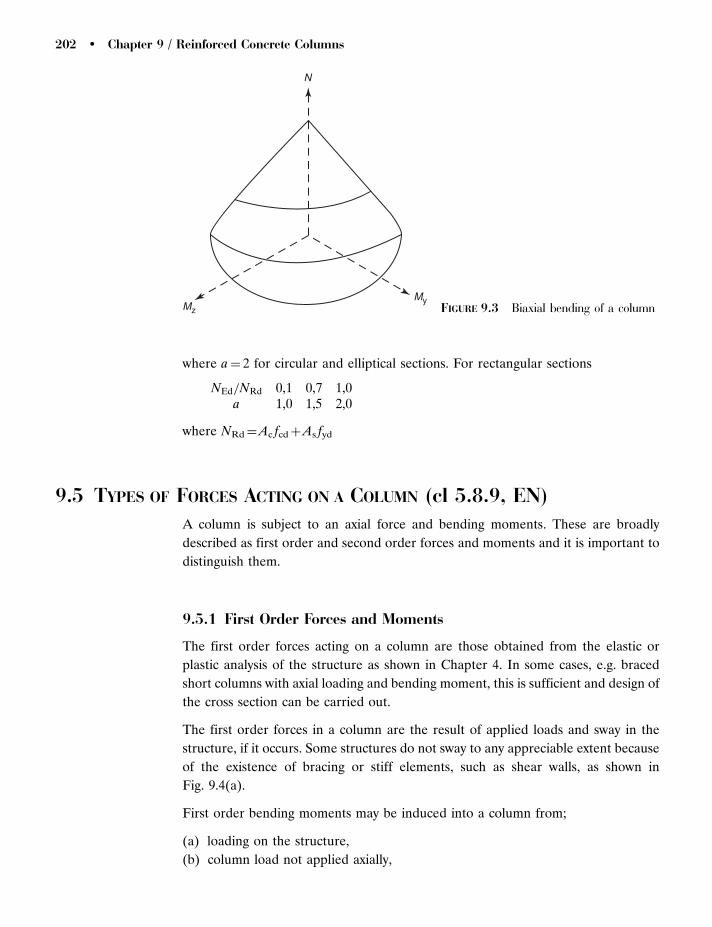
where a¼ 2 for circular and elliptical sections. For rectangular sections
NEd=NRd 0,1 0,7 1,0a 1,0 1,5 2,0
where NRd¼Ac fcdþAs fyd
9.5 TYPES OF FORCES ACTING ON A COLUMN (cl 5.8.9, EN)A column is subject to an axial force and bending moments. These are broadly
described as first order and second order forces and moments and it is important to
distinguish them.
9.5.1 First Order Forces and Moments
The first order forces acting on a column are those obtained from the elastic or
plastic analysis of the structure as shown in Chapter 4. In some cases, e.g. braced
short columns with axial loading and bending moment, this is sufficient and design of
the cross section can be carried out.
The first order forces in a column are the result of applied loads and sway in the
structure, if it occurs. Some structures do not sway to any appreciable extent because
of the existence of bracing or stiff elements, such as shear walls, as shown in
Fig. 9.4(a).
First order bending moments may be induced into a column from;
(a) loading on the structure,
(b) column load not applied axially,
N
Mz
MyFIGURE 9.3 Biaxial bending of a column
202 � Chapter 9 / Reinforced Concrete Columns
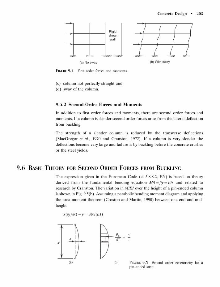
(c) column not perfectly straight and
(d) sway of the column.
9.5.2 Second Order Forces and Moments
In addition to first order forces and moments, there are second order forces and
moments. If a column is slender second order forces arise from the lateral deflection
from buckling.
The strength of a slender column is reduced by the transverse deflections
(MacGregor et al., 1970 and Cranston, 1972). If a column is very slender the
deflections become very large and failure is by buckling before the concrete crushes
or the steel yields.
9.6 BASIC THEORY FOR SECOND ORDER FORCES FROM BUCKLING
The expression given in the European Code (cl 5.8.8.2, EN) is based on theory
derived from the fundamental bending equation M/l¼ f/y¼E/r and related to
research by Cranston. The variation in M/EI over the height of a pin-ended column
is shown in Fig. 9.5(b). Assuming a parabolic bending moment diagram and applying
the area moment theorem (Croxton and Martin, 1990) between one end and mid-
height
xð�y=�xÞ � y ¼ Ax=ðEIÞ
Rigidshearwall
(a) No sway (b) With sway
FIGURE 9.4 First order forces and moments
(a) (b)
PeEI
=e
l o
1r
FIGURE 9.5 Second order eccentricity for apin-ended strut
Concrete Design � 203

hence the lateral deflection
e ¼ ð2=3Þðlo=2Þð1=rÞð5=8Þðlo=2Þ ¼ 5=48l2oð1=rÞ ð9:9Þ
The lateral deflection (e), which introduces a second order moment Ne, must be
taken into account when designing a slender column. The factor of 5/48 is
approximately the factor of 1/c¼ 1/10 in the European Code. The curvature
1/r¼ f/(Ey)¼ "/(h/2) are values given in the code (cl 5.8.8.2, EN). An additional
factor is introduced to allow for non-elastic behaviour such as creep and cracking.
9.6.1 Methods for Accounting for Second Order Forces
If second order effects are taken into account then there is a choice of methods.
(a) General method: This includes first and second order effects and is based on
non-linear analysis, including geometric non-linearity i.e. second order effects,
cracking and creep (cl 5.8.5, EN).
(b) Second order analysis based on nominal stiffness (cl 5.8.7, EN). Nominal values
of flexural stiffness are used, taking into account material non-linearity, cracking
and creep.
(c) Method based on nominal curvature (cl 5.8.8.1, EN). Suitable for isolated
members with constant normal force and effective lengths. The method gives a
second order moment (M2) based on deflection, which is related to effective
length and an estimated maximum curvature. The design moment
MEd¼MOEd þM2, where MOEd is the first order moment and M2 is the second
order moment.
9.6.2 Conditions for Ignoring Second Order Effects
If a column is short and the axial load and the first order moment are small then
second order effects can be ignored if, the
(a) second order moments are less than 10 per cent of the corresponding first order
effects (cl 5.8.2(6), EN),
(b) slenderness of a member (�) is less than a prescribed value (cl 5.8.3.1(1), EN).
(c) total vertical load is limited (cl 5.8.3.3(1), EN).
9.6.3 Columns Subject to Axial Load and Biaxial Bending (5.8.9, EN)
Some columns are subject to biaxial bending e.g. a corner column. For a complete
analysis the general method may be used. This includes first and second order
204 � Chapter 9 / Reinforced Concrete Columns
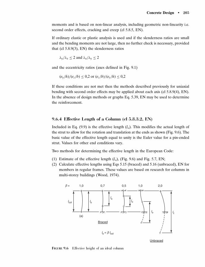
moments and is based on non-linear analysis, including geometric non-linearity i.e.
second order effects, cracking and creep (cl 5.8.5, EN).
If ordinary elastic or plastic analysis is used and if the slenderness ratios are small
and the bending moments are not large, then no further check is necessary, provided
that (cl 5.8.9(3), EN) the slenderness ratios
�y=�z � 2 and �z=�y � 2
and the eccentricity ratios (axes defined in Fig. 9.1)
ðey=hÞ=ðez=bÞ � 0,2 or ðez=bÞ=ðey=hÞ � 0,2
If these conditions are not met then the methods described previously for uniaxial
bending with second order effects may be applied about each axis (cl 5.8.9(4), EN).
In the absence of design methods or graphs Eq. 5.39, EN may be used to determine
the reinforcement.
9.6.4 Effective Length of a Column (cl 5.8.3.2, EN)
Included in Eq. (9.9) is the effective length (lo). This modifies the actual length of
the strut to allow for the rotation and translation at the ends as shown (Fig. 9.6). The
basic value of the effective length equal to unity is the Euler value for a pin-ended
strut. Values for other end conditions vary.
Two methods for determining the effective length in the European Code:
(1) Estimate of the effective length (lo), (Fig. 9.6) and Fig. 5.7, EN;
(2) Calculate effective lengths using Eqs 5.15 (braced) and 5.16 (unbraced), EN for
members in regular frames. These values are based on research for columns in
multi-storey buildings (Wood, 1974).
b =
lo = b lcol
1,0
lcol lo
lolo
lo lo
0,7 0,5 1,0
Braced
Unbraced
(a)
2,0
FIGURE 9.6 Effective height of an ideal column
Concrete Design � 205

9.6.5 Slenderness Ratio of a Column (cl 5.8.3.2, EN)
A better measure of the susceptibility to buckling is the slenderness ratio which
includes section properties of the column. The slenderness ratio
� ¼ ðeffective length)/(radius of gyration) ¼ lo=i ¼ lolðI=AÞ0,5
ð9:10Þ
For rectangular sections, cross-sectional area b� h, bending about the major axis,
ignoring the steel reinforcement, the radius of gyration
i ¼ ðI=AÞ0,5¼ ðbh3=12bhÞ0,5
¼ h=ð2 � 30,5Þ ð9:11Þ
9.7 SUMMARY OF THE DESIGN METHOD FOR COLUMNS SUBJECTTO AXIAL LOAD AND BENDING
Assuming that an elastic or plastic analysis of the structure has been carried out
which gives only primary moments.
(1) Assume a size of column and material strengths for concrete and steel.
(2) Determine the first order moment (MOEd) about the major axis based on the
plastic or elastic analysis, of part, or whole of the structure.
(3) Check if first order moment about the major axis and eccentricity can be
ignored.
(4) Assume area of longitudinal steel and calculate the second order buckling
moment about the major axis M2¼NEde2.
(5) Check if second order moment about the major axis can be ignored.
(6) Calculate the design moment about the major axis MEd¼MOEdþM2.
(7) Confirm, or revise, the assumed area of reinforcement from a column graph
(Annex B3) which relates NEd/(bh fck) and MEd/(bh2 fck).
(8) If biaxial bending, repeat bending calculations and checks about minor axis to
determine the design moment.
(9) If biaxial bending, check whether combined actions should be considered.
(10) If no biaxial graph, use biaxial equation (MEdz/MRdz)aþ (MEdy/MRdy)
a� 1.
(11) Check limits for maximum and minimum reinforcement.
EXAMPLE 9.1 Isolated column bending about the major axis in a non-sway
structure. Determine the steel reinforcement required in column in a non-sway
structure subject to first order actions of 1750 kN axial load and a bending moment
of 100 kNm. The height of the column is 3 m.
Following the steps in Section 9.7.
Step (1) Assume section 300� 300 mm, Grade C50/60 concrete and fyk¼ 500 MPa.
Step (2) Given the first order bending moment¼ 100 kNm.
206 � Chapter 9 / Reinforced Concrete Columns

Step (3) Check if the first order bending moment4minimum (cl 6.1(4), EN)
NEdh=30 ¼ 1750 � 0,3=30 ¼ 17,55M1 ¼ 100 kNm; Use 100 kNm:
Check if first order eccentricity greater than minimum (cl 6.1(4), EN)
e1 ¼ MEd=NEd ¼ 100E3=1750 ¼ 574min: ð20Þ4h=30ð10Þmm: Use e1 ¼ 57 mm:
Step (4) Assume 4T16 (804 mm2). Apply method (Eq. 5.33, EN) based on
nominal curvature to determine the additional buckling second order moment
M2 ¼ NEde2:
Calculate the following factors to obtain a value for the second order buckling
eccentricity (e2)
Curvature (Eq. 5.34, EN)
ð1=rÞ ¼ KrK�ð1=roÞ ¼ KrK�ð fyd=EsÞ=ð0,45dÞ
¼ 0,745 � 1,37 � ð500=1,15Þ=200E3=ð0,45 � 0,85 � 300Þ ¼ 19,4E�6
Kr ¼ ðnu � nÞ=ðnu � nbalÞ ðEq: 5 :36, ENÞ
¼ ð1,117 � 0,583Þ=ð1,117 � 0,4Þ ¼ 0,74551
nu ¼ 1 þ ! ¼ 1 þ 0,117 ¼ 1,117
n ¼ NEd=ðAc fcdÞ ¼ 1750E3=ð300 � 300 � 50=1,5Þ ¼ 0,583
! ¼ As fyd=ðAc fcdÞ ¼ 804 � ð500=1,15Þ=ð300 � 300 � 50=1,5Þ ¼ 0,117
Effective creep factor (Eq. 5.37, EN)
K� ¼ 1 þ ��ef ¼ 1 þ 0,427 � 0,867 ¼ 1,3741, satisfactory:
�ef ¼ �ð�,toÞMOEqp=MOEd ¼ 1,3 � 2=3 ¼ 0,867 ðcl 5:19, ENÞ
�ð�,toÞ ¼ 1,3 ðcl 3:1:4ð2Þ, ENÞ
� ¼ 0,35 þ fck=200 � �=150 ¼ 0,35 þ 50=200 � 26=150 ¼ 0,427
Slenderness ratio (cl 5.8.3.1, EN)
� ¼ lo=i ¼ 0,75 � 3E3=½300=ð2 � 30,5� ¼ 26
Second order buckling deflection of the column (cl 5.8.8.2(4), EN)
e2 ¼ ½ð1=rÞl2o=c� ¼ 19,4E-6 � ð0,75 � 3E3Þ2=10 ¼ 9,82 mm:
Second order moment (Eq. 5.33, EN)
M2 ¼ NEde2 ¼ 1750 � 9,82 � 1E-3 ¼ 17,2 kNm:
Concrete Design � 207

Step (5) Check if the second order moment can be ignored.
Method (a) (cl 5.8.2(6), EN)
M2/MOEd ¼ 17,2/100� 100¼ 17.2%4 10%, therefore second order moment cannot
be ignored.
Method (b) (cl 5.8.3.1, EN)
� ¼ 26
A ¼ 1=ð1 þ 0,2�efÞ ¼ 1=ð1 þ 0,2 � 0,867Þ ¼ 0,852
B ¼ ð1 þ 2!Þ0,5¼ ð1 þ 2 � 0,117Þ0,5
¼ 1,11
C ¼ 1,7 � rm ¼ 1,7 �M01=M02 ¼ 1,7 � 0,7 ¼ 1
n ¼ NEd=ðAc fcdÞ ¼ 1750E3=ð300 � 300 � 50=1,5Þ ¼ 0,583
�lim ¼ 20ABC=n0,5 ¼ 20 � 0,852 � 1,11 � 1=0,5830,5 ¼ 24,8
�(26)5 �lim(24,8), therefore second order effects cannot be ignored. Method(c)
(cl 5.8.3.3, EN) is not applicable to this structure.
Step (6) Design values.
NEd ¼ 1750 kN, and MEd ¼ M1 þM2 ¼ 100 þ 17,2 ¼ 117,2 kNm:
Step (7) Reinforcement is determined from the design graph (Annex B3)
MEd=ðhb2fckÞ ¼ 117,2E6=ð300 � 3002 � 50Þ ¼ 0,0868
NEd=ðbhfckÞ ¼ 1750E3=ð300 � 300 � 50Þ ¼ 0,389
d=h ¼ ð300 � 30 � 16=2Þ=300 ¼ 0,873:
From graph, for d/h¼ 0,85 and fck¼ 50 MPa
�¼Asc fy/(bhfck)¼ 0,5 and hence
Asc,req ¼ 0,05 � 3002 � 50=500 ¼ 4505ð4T16Þ804 mm2, acceptable.
Use 4T16 longitudinal corner bars (804 mm2).
Steps (8) to (10) Ignore because no biaxial bending.
Step (11) Check limits for reinforcement.
Maximum reinforcement ratio (cl 9.5.2(3), EN)
As ¼ 8045Asc, max ¼ 0,04 � 3002 ¼ 3600 mm2, satisfactory
Minimum reinforcement ratio (cl 9.5.2.(2), EN)
As, min ¼ 0,10NEd=fyd ¼ 0,10 � 1750E3=ð500=1,15Þ
¼ 402,55ð4T16Þ804 mm2, satisfactory
208 � Chapter 9 / Reinforced Concrete Columns

or
0,002Ac ¼ 0,002 � 3002 ¼ 1805ð4T16Þ804 mm2, satisfactory:
Transverse reinforcement (cl 9.5.3(3), EN)
�=4 ¼ 16=4 ¼ 456, use 6 mm:
Spacing of transverse reinforcement (cl 9.5.3(3), EN) the lesser value of
scl,tmax¼ 20�¼ 20� 16¼ 320 mm; or b¼ 300 mm; or 400 mm, Use s¼ 300 mm
EXAMPLE 9.2 Column subject to biaxial bending. A column in the bottom storey
of a building sways in bending about the z-z axis but shear walls prevent sway about
the y-y axis (Fig. 9.7).
Following the steps in section 9.7.
Step (1) Assume section 400� 800 mm, C50/60 Grade concrete and fyk ¼ 500 MPa.
Step (2) From an elastic analysis the axial load is 2000 kN and the first order
moments at the ends of the column are as shown (Fig. 9.7). This analysis does not
give second order bending moments.
Step (3) Check if the first order bending moment4minimum (cl 6.1(4), EN)
NEd h=30 ¼ 2000 � 0,8=30 ¼ 53,35M1 ¼ 150 kNm, Use 150 kNm:
Check if first order eccentricity is greater than minimum (cl 6.1(4), EN)
e1 ¼ MEd=NEd ¼ 150E3=2000 ¼ 754min: ð20Þ4h=30ð800=30 ¼ 26; 7Þmm,
Use e1 ¼ 75 mm
150
A
B
ZZ-Z axis Y-Y axis
Z
Y
First order bending moments
Y
125
4,5
m
15 kNm
9 kNm
FIGURE 9.7 Example: column in biaxial bending
Concrete Design � 209

Step (4) Assume 8T25 (3927 mm2). Determine the second order bending
(M2z¼NEde2z) about the z-z axis based on nominal curvature (Eq. 5.33, EN).
Calculate the following to obtain a value for the second order deflection of the
column (e2z).
Estimated effective length of column bending about the z-z axis (Fig. 9.4)
lo ¼ 1,5 � 4,5 ¼ 6,75 m
�z ¼ lo=iz ¼ 6,75E3=½800=ð2 � 30,5Þ� ¼ 29;2:
Curvature (Eq. 5.34, EN)
ð1=rÞ ¼ KrK�ð1=roÞ ¼ KrK�ð fyd=EsÞ=ð0,45dÞ
¼ 1 � 1,25 � ð500=1,15Þ=200E3=ð0,45 � 0,85 � 800Þ ¼ 8,88E-6
which necessitates calculating the following factors (Eq. 5.36, EN)
Kr ¼ ðnu � nÞ=ðnu � nbalÞ ¼ ð1,16 � 0,188Þ=ð1,16 � 0,4Þ
¼ 1,2841, use 1 ðEq: 5:36, ENÞ
nu ¼ 1 þ ! ¼ 1 þ 0,16 ¼ 1,16
n ¼ NEd=ðAc fcdÞ ¼ 2000E3=ð400 � 800 � 50=1,5Þ ¼ 0,188
assuming 8T25 (3927 mm2)
! ¼ As fyd=ðAc fcdÞ ¼ 3927 � ð500=1,15Þ=ð400 � 800 � 50=1,5Þ ¼ 0,16
Effective creep factor (Eq. 5.37, EN)
K� ¼ 1 þ ��ef ¼ 1 þ 0,405 � 0,867 ¼ 1,354 1, satisfactory:
�ef ¼ �ð�,toÞ MOEqp=MOEd ¼ 1,3 � 2=3 ¼ 0,867 ðEq: 5:19, ENÞ
�ð�,toÞ ¼ 1,3 ðcl 3:1:4ð2Þ, ENÞ
� ¼ 0,35 þ fck=200 � �=150 ¼ 0,35 þ 50=200 � 29,2=150 ¼ 0,405
Second order buckling deflection of column (cl 5.8.8.2(4), EN)
e2z ¼ ð1=rÞl2o=c ¼ 8,88E-6 � ð1,5 � 4,5E3Þ2=10 ¼ 40,5 mm:
Second order moment about the z-z axis (Eq. 5.33, EN)
M2z ¼ NEde2z ¼ 2000 � 40,5 � 1E-3 ¼ 81 kNm:
210 � Chapter 9 / Reinforced Concrete Columns
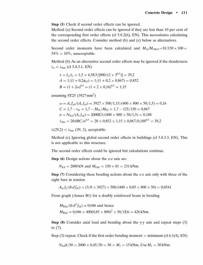
Step (5) Check if second order effects can be ignored.
Method (a) Second order effects can be ignored if they are less than 10 per cent of
the corresponding first order effects (cl 5.8.2(6), EN). This necessitates calculating
the second order effects. Consider method (b) and (c) below as alternatives.
Second order moments have been calculated and M2z/MOEd ¼ 81/150� 100¼
54%4 10%, unacceptable.
Method (b) As an alternative second order effects may be ignored if the slenderness
�z5 �lim (cl 5.8.3.1, EN)
� ¼ lo=iz ¼ 1,5 � 4,5E3=½800=ð2 � 30,5Þ� ¼ 29,2
A ¼ 1=ð1 þ 0,2�efÞ ¼ 1=ð1 þ 0,2 � 0,867Þ ¼ 0,852
B ¼ ð1 þ 2!Þ0,5¼ ð1 þ 2 � 0,16Þ0,5
¼ 1,15
assuming 8T25 (3927 mm2)
! ¼ As fyd=ðAc fcdÞ ¼ 3927 � 500=1,15=ð400 � 800 � 50=1,5Þ ¼ 0,16
C ¼ 1,7 � rm ¼ 1,7 �M01=M02 ¼ 1,7 � 125=150 ¼ 0,867
n ¼ NEd=ðAc fcdÞ ¼ 2000E3=ð400 � 800 � 50=1,5Þ ¼ 0,188
�lim ¼ 20ABC=n0,5 ¼ 20 � 0,852 � 1,15 � 0,867=0,1880,5 ¼ 39,2
�(29,2)5 �lim (39, 2), acceptable.
Method (c) Ignoring global second order effects in buildings (cl 5.8.3.3, EN). This
is not applicable to this structure.
The second order effects could be ignored but calculations continue.
Step (6) Design actions about the z-z axis are
NEd ¼ 2000 kN and MEdz ¼ 150 þ 81 ¼ 231 kNm:
Step (7) Considering these bending actions about the z-z axis only with three of the
eight bars in tension
Asc fy=ðb d fckÞ ¼ ð3=8 � 3927Þ � 500=ð400 � 0,85 � 800 � 50Þ ¼ 0,0541
From graph (Annex B1) for a doubly reinforced beam in bending
MRdz=ðb d2 fckÞ ¼ 0,046 and hence
MRdz ¼ 0,046 � 400ð0,85 � 800Þ2 � 50=1E6 ¼ 426 kNm:
Step (8) Consider axial load and bending about the y-y axis and repeat steps (3)
to (7).
Step (3) repeat. Check if the first order bending moment4minimum (cl 6.1(4), EN)
NEdh=30 ¼ 2000 � 0,45=30 ¼ 304M1 ¼ 15 kNm, UseM1 ¼ 30 kNm:
Concrete Design � 211

Check if first order eccentricity is greater than minimum (cl 6.1(4), EN)
e1 ¼ MEd=NEd ¼ 15E3=2000 ¼ 7,55h=30ð400=30 ¼ 13,3Þ5min: ð20Þmm, Use e1
¼ 20 mm and M1 ¼ 20 � 2E3 ¼ 40 kNm:
Estimated effective length of column bending about the y-y axis (Fig. 9.4)
lo¼ 0,75� 4,5¼ 3,375 m.
Slenderness ratio
�y ¼ lo=iy ¼ 3,375E3=½400=ð2 � 30,5Þ� ¼ 29,2:
Step (4) repeat. Determine the second order bending (M2¼NEde2y) about the y-y
axis based on nominal curvature (Eq. 5.33, EN). The following quantities need to be
calculated to obtain a value for the deflection of the column (e2y)
Curvature (Eq. 5.34, EN)
ð1=rÞ ¼ KrK�ð1=roÞ ¼ KrK�ð fyd=EsÞ=ð0,45dÞ
¼ 1 � 1,25 � ð500=1,15Þ=200E3=ð0,45 � 0,85 � 400Þ ¼ 17,8E� 6
which includes factors (Eq. 5.36, EN)
Kr ¼ ðnu � nÞ=ðnu � nbalÞ ¼ ð1,16 � 0,188Þ=ð1,16 � 0,4Þ ¼ 1,2841, Use 1
nu ¼ 1 þ ! ¼ 1 þ 0,16 ¼ 1,16
n ¼ NEd=ðAc fcdÞ ¼ 2000E3=ð400 � 800 � 50=1,5Þ ¼ 0,188
! ¼ As fyd=ðAc fcdÞ ¼ 3927 � ð500=1,15Þ=ð400 � 800 � 50=1,5Þ ¼ 0,16
Effective creep factor (Eq. 5.37, EN)
K� ¼ 1 þ ��ef ¼ 1 þ 0,405 � 0,867 ¼ 1,3541, satisfactory:
which includes
�ef ¼ �ð�,toÞMOEqp=MOEd ¼ 1,3 � 2=3 ¼ 0,867 ðEq: 5:19, ENÞ
�ð�,toÞ ¼ 1,3 ðcl 3:1:4ð2Þ, ENÞ
� ¼ 0,35 þ fck=200 � �=150 ¼ 0,35 þ 50=200 � 29,2=150 ¼ 0,405
Buckling deflection of strut (cl 5.8.8.2(4), EN)
e2y ¼ ð1=rÞl2o=c ¼ 17; 8E-6 � ð0,75 � 4,5E3Þ2=10 ¼ 20,3 mm:
Second order moment about the y-y axis (Eq. 5.33, EN)
M2y ¼ NEde2y ¼ 2000 � 20,3 � 1E-3 ¼ 40,6 kNm:
212 � Chapter 9 / Reinforced Concrete Columns
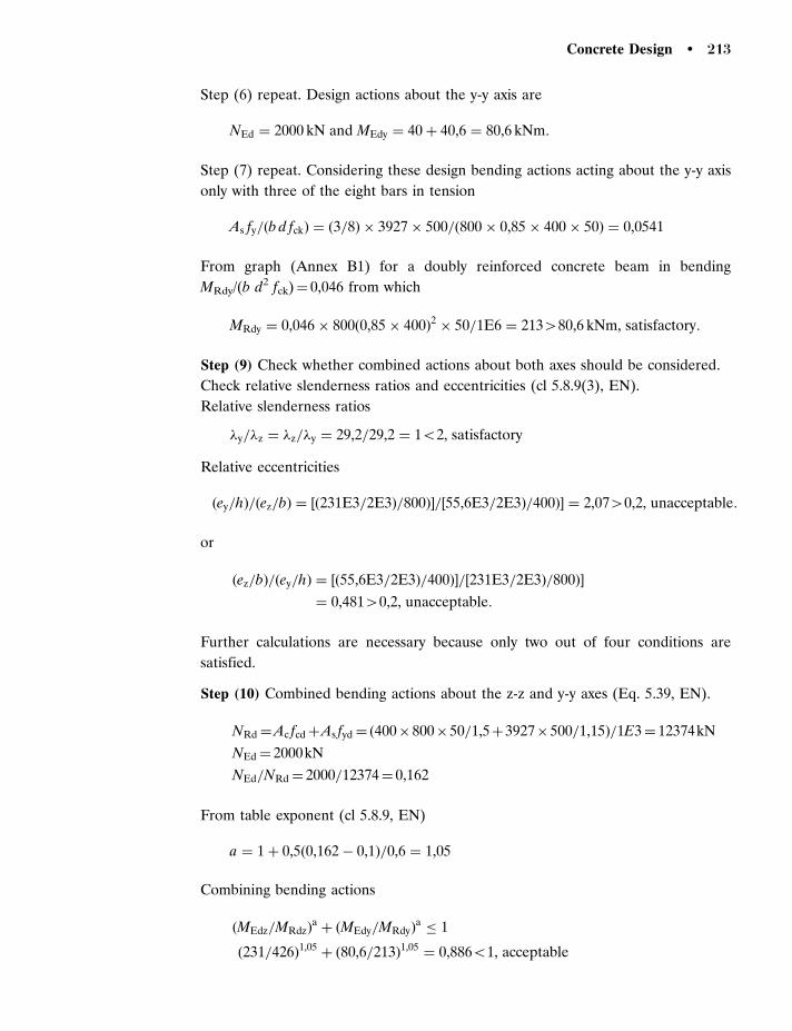
Step (6) repeat. Design actions about the y-y axis are
NEd ¼ 2000 kN and MEdy ¼ 40 þ 40,6 ¼ 80,6 kNm:
Step (7) repeat. Considering these design bending actions acting about the y-y axis
only with three of the eight bars in tension
As fy=ðb d fckÞ ¼ ð3=8Þ � 3927 � 500=ð800 � 0,85 � 400 � 50Þ ¼ 0,0541
From graph (Annex B1) for a doubly reinforced concrete beam in bending
MRdy/(b d2 fck)¼ 0,046 from which
MRdy ¼ 0,046 � 800ð0,85 � 400Þ2 � 50=1E6 ¼ 213480,6 kNm, satisfactory:
Step (9) Check whether combined actions about both axes should be considered.
Check relative slenderness ratios and eccentricities (cl 5.8.9(3), EN).
Relative slenderness ratios
�y=�z ¼ �z=�y ¼ 29,2=29,2 ¼ 152, satisfactory
Relative eccentricities
ðey=hÞ=ðez=bÞ ¼ ½ð231E3=2E3Þ=800Þ�=½55,6E3=2E3Þ=400Þ� ¼ 2,0740,2, unacceptable:
or
ðez=bÞ=ðey=hÞ ¼ ½ð55,6E3=2E3Þ=400Þ�=½231E3=2E3Þ=800Þ�
¼ 0,48140,2, unacceptable:
Further calculations are necessary because only two out of four conditions are
satisfied.
Step (10) Combined bending actions about the z-z and y-y axes (Eq. 5.39, EN).
NRd ¼Ac fcd þAs fyd ¼ ð400�800�50=1,5þ3927�500=1,15Þ=1E3¼ 12374kN
NEd ¼ 2000kN
NEd=NRd ¼ 2000=12374¼ 0,162
From table exponent (cl 5.8.9, EN)
a ¼ 1 þ 0,5ð0,162 � 0,1Þ=0,6 ¼ 1,05
Combining bending actions
ðMEdz=MRdzÞaþ ðMEdy=MRdyÞ
a� 1
ð231=426Þ1,05þ ð80,6=213Þ1,05
¼ 0,88651, acceptable
Concrete Design � 213
Use 8T25 (3927 mm2) longitudinal bars.
Step (11) Check limits for reinforcement
Check maximum reinforcement ratio (cl 9.5.2(3), EN)
As ¼ 39275As, max ¼ 0,04 � 400 � 800 ¼ 12800 mm2, satisfactory
Check minimum reinforcement ratio (cl 9.5.2(2), EN)
As, min ¼ 0,10NEd=fyd ¼ 0,10 � 2000E3=ð500=1,15Þ ¼ 46053927 mm2, acceptable
or
0,002Ac ¼ 0,002 � 400 � 800 ¼ 64053927 mm2, satisfactory:
Transverse reinforcement (cl 9.5.3(3), EN)
�=4 ¼ 25=4 ¼ 6,2546, use 8 mm:
Spacing of transverse reinforcement (cl 9.5.3(3), EN) the lesser value of
scl,tmax¼ 20�¼ 20� 25¼ 500 mm; or b¼ 400 mm; or 400 mm; use s¼ 400 mm.
REFERENCES AND FURTHER READING
ACI-ASCE Committee 441(1966). Reinforced concrete columns. ACI Pub. SP-13.
Bresler B. (1960). Design criteria for reinforced concrete columns under axial load and bending.
Proc. ACI, 57, No. 5, Nov.
Cranston, W.B. (1972). Analysis and design of reinforced concrete columns. C and C. Assoc.
Research Report No. 20.
Croxton, P.C.L. and Martin, L.H. (1990). Solving Problems in Structures. Longman Scientific and
Technical.
Furlong, R.W. (1961). Ultimate strength of square columns under biaxially eccentric loads.
Proc. ACI, 57, No. 9, March.
MacGregor, J.D., Breen, J.E. and Pfrang, E.O. (1970) Design of slender concrete columns.
Proc. ACI, 67, No. 1, January.
Pannel, F.N. (1963). Failure surfaces for members in compression and biaxial bending. ACI Jnl.,
Proc. Vol. 60, No. 1.
Warner, R.F. (1969). Biaxial Moment thrust curvature relations. Jnl. Struct. Div., ASCE, Vol. 95,
No. ST5.
Wood, R.H. (1974). Effective lengths of columns in multi-storey buildings. Struct. Eng., Vol. 52,
No. 7, July.
214 � Chapter 9 / Reinforced Concrete Columns

C h a p t e r 10 / Reinforced Concrete Slabs
This chapter covers design of slabs and provides an introduction to both Yield Line
and Hillerborg Strip Methods. The definition of a slab is when the panel width
is substantially greater than 5 times the overall slab thickness (cl 5.3.1 (4)). This
distinction is unimportant for flexural design except that it is customary to consider
unit widths in the calculations but becomes potentially critical for shear especially
punching shear around columns for flat slabs.
10.1 TYPES OF SLABThe various types of slab are illustrated in Fig. 10.1. The simplest type of slab is solid
and of uniform thickness. This type of slab is potentially uneconomic in terms of
efficient usage of materials owing to the inherent high ratio of permanent to variable
actions. It is however relatively simple to construct as it has a flat soffit.
For large areas of slab, it is necessary to consider ways in which the self weight of the
slab can be reduced without compromising its load carrying capacity. This reduction
can be achieved in one of the two ways. The first is to place voids in the soffit of slab
and thus creating a regular pattern of ribs in both directions. This type of slab is
known as a waffle or coffered slab. The portions round the columns are left solid to
counteract the effect of punching shear and to enhance resistance to hogging
moments. Such slabs are often left with exposed soffits. The second method is to
reduce the thickness of slab over most of the span where the shear is low but to keep
an increased thickness at the support. Such a system is called a flat slab with drop-
heads around the columns.

10.2 DESIGN PHILOSOPHIES
10.2.1 Ultimate Limit States (cl 2.5.3.5.2)
A series of methods are available to determine the internal stress resultants:
(1) The Principles in Cl 5.5 indicate that linear elastic analysis with or without
redistribution of moments, subject to limits on the neutral axis depths and the
ratio between lengths of adjacent spans must lie between 0,5 and 2 if no check
is to be made on rotation capacity.
(2) Section 5.6 indicates Upper or lower bound plastic methods may be used subject
to the conditions that xu is limited to 0,25 for concrete strength classes less
than C50/60 or 0,15 above this value, the reinforcement is Class B or C, and the
ratio of moments at intermediate supports to the span moments should lie
between 0,5 and 2, and
(3) Non-linear numerical approaches. In practice the most common methods are
the Johansen Yield Line approach which corresponds to an Upper Bound
plastic method, the Hillerborg Strip to a Lower Bound plastic method and
Finite Element Analysis (FEA). A linear elastic analysis may either be based on
longitudinal and transverse frames or FEA loaded at ultimate limit state and the
design then carried out on the resulting moments and shears. Non-linear
analysis will not be considered.
Beeby (2004) indicates that currently high yield reinforcement of sizes below 16 mm
may be Class A owing to their method of manufacture. Since smaller bar sizes than
this are more likely to be used in slabs, it is essential where plastic methods are used
for the analysis that Class B or C reinforcement is specified and that this is checked
(a) Solid slab
Colum centreline
(b) Ribbed slab
(c) Flat slab with drophead FIGURE 10.1 Types of slab
216 � Chapter 10 / Reinforced Concrete Slabs

on site before the reinforcement is fixed or concreting has commenced. It is
suggested that even for the Hillerborg Strip Method, Class B or C should specified.
10.2.2 Serviceability Limit States
As deemed to satisfy, clauses are normally used to design against excessive deflection
or cracking a full analysis is rarely necessary.
10.3 PLASTIC METHODS OF ANALYSISFor a plastic method of analysis to give the true collapse load the following three
criteria must, by the uniqueness theorem, be satisfied:
� Equilibrium
The internal forces, or stress resultants, must be in equilibrium with the applied
loading.
� Yield
The moments in any part of the structure must be less than or equal to the
ultimate, or yield, moment at that point in the structure.
� Mechanism Formation
In order that partial or total collapse can occur, a mechanism must occur.
For a frame structure comprising linear elements it is relatively easy to determine a
situation which satisfies all the three criteria. For slabs it is less easy, and therefore
acceptable methods which satisfy only two of the criteria have been developed. Each
of these methods must satisfy equilibrium. It is NOT permissible to generate
solutions which are not in equilibrium with the applied loading.
10.3.1 Lower Bound Solution
Here a set of moments are found which are in equilibrium with the applied loading
and satisfy the yield criterion. Such a set of moments will not cause collapse to occur.
An example of such a solution is the result of an elastic analysis under ultimate loads
with no redistribution. A design method was formulated by Hillerborg and is known
as the Hillerborg Strip Method (Wood and Armer, 1968).
10.3.2 Upper Bound Solution
A set of moments is found that are in equilibrium and form mechanisms but which
may violate the yield criterion. This type of solution was studied extensively by
Concrete Design � 217

Johansen and gave rise to the Johansen Yield Line Method (Johansen, 1972). Each
of these methods will be considered in turn.
10.4 JOHANSEN YIELD LINE METHOD
It has been observed in tests that when slabs are loaded to failure, large cracks occur
normal to the directions of maximum moments. These cracks are observed only on
the tension zones of the slab and are caused by the reinforcement yielding and large
ductile rotations occurring (similar to those in under-reinforced beams). The
sections between the yield lines undergo rigid body rotation (or displacement) and
thus the concept of a failure mechanism can be postulated. Although the yield line
approach is an upper bound solution in that a yield criterion is not checked, the
results from such an analysis are satisfactory since the analysis ignores both the
effects of strain hardening in the reinforcement as the reinforced concrete slab is
assumed to behave as a rigid, elastic, perfectly plastic material and any beneficial
effect generated by membrane action caused by in-plane forces in the slab. Both
these phenomena increase the load carrying capacity beyond the level calculated,
assuming the loading is carried by flexure to the extent that the calculated load
carrying capacity is below the actual. It is essential that all potential mechanisms are
checked especially where point loads occur or where a sagging yield line intersects
the angle between two hogging yield lines.
10.4.1 Methodology
A possible yield mechanism is proposed and the load that may be carried is
determined in terms of the moment capacity of the slab, or the moment field
required is calculated in terms of a predetermined loading. It is often necessary to
characterize the yield line pattern by a series of unknown dimensions. Symmetry and
the existence of point loads may fix some of the yield line patterns. The resultant
algebraic expressions involving the loading, moment field and unknown dimensions
may be solved by either explicit solutions in relatively simple cases or by numerical
techniques or spreadsheets where an explicit solution is not possible or difficult.
There are two methods of determining the inter-relations between the loading,
moments and yield line patterns: Virtual work approach or Nodal force approach.
10.4.2 Virtual Work Approach
In this method, the equilibrium equation is set up by imposing virtual deformations
to the yield lines and determining the (virtual) work done by the loads and the
moments.
218 � Chapter 10 / Reinforced Concrete Slabs
10.4.3 Nodal Force Approach
In this method, nodal forces due to internal shears are calculated at the points where
the yield lines intersect, other than under point loads or at supports. Equilibrium
equations are then formulated for each portion of the slab, the unknown dimensions
characterizing the yield lines eliminated and the resultant relationship between the
loads and moments determined.
Attention was drawn earlier to the situation where a sagging yield line intersects the
angle between two hogging yield lines. In this situation the yield criterion is auto-
matically violated and thus alternatives need to be sought. It should be noted that
such alternatives often involve the use of curved rather than straight yield lines. The
situation involving the intersection of hogging and sagging yield lines may however
often produce a solution which is still acceptable in terms of the needs of design.
10.4.4 Postulation of the Layout of Yield Line Mechanisms
A basic series of rules were laid out by Johansen (1972) for situations not involving
the formation of curved yield lines:
(i) Yield lines are normally straight and form axes of rotation.
(ii) Yield lines must terminate at a boundary unless parallel to a support.
(iii) Axes of rotation coincide with simply supported edges, cut free edges and pass
over column supports.
(iv) Axes of rotation of adjacent regions must either meet at a point or be parallel.
(v) Hogging yield lines will form along encastre supports.
The examples shown in Fig. 10.2 illustrate the application of these rules.
Note, in all the examples on yield line and Hillerborg strip, the conventional notation
of m with no subscripts has been retained for the moment per unit width.
Reinforcement is generally provided in an orthogonal pattern (unless the slab is a
very odd shape) and thus a yield line is likely to intersect the reinforcement at an
angle (Fig. 10.3).
If the reinforcement in a particular direction has a moment of resistance m per
unit width normal to the direction of the reinforcement, the moment across the
yield line mn1 can be obtained by resolving forces,
mn1 L ¼ mRdðL sin �Þ½ � sin � ð10:1Þ
or
mn1 ¼ mRd sin2 � ð10:2Þ
Concrete Design � 219

If there is an additional reinforcement orthogonal to the first with a moment of
resistance �mRd, then the contribution of this reinforcement to the moment across
the yield line mn2 is
mn2 ¼ �mRd sin2ð90 � �Þ ð10:3Þ
Total moment across the yield line mn is given by the sum of the contributions mn1
and mn2 from Eqs (10.2) and (10.3), or
mn ¼ mRd sin2 � þ �mRd sin2ð90 � �Þ ð10:4Þ
If as is usual, the reinforcement is isotropic (�¼ 1), then
mn ¼ mRd ð10:5Þ
Key
Axis of rotation
Free edge
Simply supported edge
Encastré edge
Yield line
Column support
FIGURE 10.2 Some typical yield linepatterns
220 � Chapter 10 / Reinforced Concrete Slabs

To determine the work done by the yield line consider the yield line xy in Fig. 10.4.
The work done may be stated as the moment times the rotation times the projected
length of the yield line on the axis of rotation, so for yield line xy, the work done is
m�(length x0y0)��. The alternative approach is to use the moment normal to the
yield line given by Eqs (10.4) or (10.5) and the work done calculated as the normal
moment times the length of the yield line times the total rotational angle.
To determine the angles of rotation, it is a general practice to impose (virtual)
displacements of unity on the yield line undergoing the maximum displacement.
The work done by the loads is simply calculated as load times (virtual) displacement
for a point load and the total load times the (virtual) displacement of the centroid of
the load for either uniform line loads (loads per unit length) or uniformly distributed
loads (loads per unit area). For uniformly distributed loads, the work done is also
Yield line
Reinforcement
(kNm/m width)
mL
x
y
C
A
O
OA
Section C - C
y ′
x ′
mn
z
z
q
C
L s
in q
f
FIGURE 10.3 Formation of yield lines inclined to the reinforcement
Axisof rotation
xx ′
y ′
m
mMomentfield
y
f
FIGURE 10.4 Work done by yield lines
Concrete Design � 221

given by the load times the volume between the original slab and its displaced shape.
For non-uniform loads, it will be necessary to carry out integration to determine
the work done.
A series of examples will now be undertaken. In all cases an encastre slab will be
analysed since the solution for a simply supported slab can be obtained by setting the
moment parameter i defining the encastre moment equal to zero.
EXAMPLE 10.1 Square slab. Consider a square slab of side L carrying a UDL at
ultimate limit state of n per unit area (Fig. 10.5(a)). The slab has isotropic orthogonal
reinforcement giving sagging moments of resistance m per unit run and hogging im.
The only possible configuration using simple straight yield lines is that shown in
Fig. 10.5(b). Owing to symmetry on a quarter of the slab need be considered.
A B
A B
O
O
O ′A B
D C
(a) Slab details
(b) Yield line pattern
Axis of
rotation
(c) Moments on section AOB
D C
L
im
im im
im
im
mm
m
n = load/unitarea
FIGURE 10.5 Yield line collapse foran encastre square slab
222 � Chapter 10 / Reinforced Concrete Slabs

Using virtual work and giving the centre of the slab O a displacement of unity, the
internal work done by the moments can be determined as follows:
Sagging yield Line:
Yield Line AO:
moment per unit run: m
Projected length of AO: AO0 ¼L/2
Rotation: �¼ 1/OO0 ¼ 1/(L/2)¼ 2/L
W :D: ¼ mL
2
1
L=2¼ m ð10:6Þ
Yield Line OB:
This is identical to yield line AO, so work done¼mRd
Thus total work done by sagging yield line
W :D: ¼ 2m ð10:7Þ
Hogging yield line:
moment: im
Projected length of AB: AB¼L
Rotation: �¼ 1/(L/2)¼ 2/L
W :D: ¼ imL1
L=2¼ 2im ð10:8Þ
Total work done by hogging and sagging yield lines from Eqs (10.7) and (10.8)
is given by
W :D: ¼ 2mþ 2im ¼ 2ðiþ 1Þm ð10:9Þ
Work done by loads:
Displaced volume between original and deflected slab for one-quarter of the slab is
(1/4)(1�L2/3)¼L2/12.
W :D: ¼ nL2
12ð10:10Þ
Equating internal and external work done from Eqs (10.9) and (10.10) gives
2ðiþ 1Þm ¼nL2
12ð10:11Þ
or
m ¼nL2
24ðiþ 1Þð10:12Þ
Concrete Design � 223

Note that this is a classic case where the yield criterion is violated at the corner
(Jones and Wood, 1967). Alternative solutions are given in Example 10.9.
EXAMPLE 10.2 Rectangular slab encastre on all edges under a UDL of n per unit
area. The geometry and collapse mechanism are given in Fig. 10.6(a) and (b). The
yield line position is characterized by the length �L and the yield line FG is displaced
by unity vertically downwards. Consider half the slab i.e. region ABFGD.
Work done by loads:
Volume displaced (for half the slab).
Volume under the pyramid in region AFB,
VI ¼1
3ð�L�LÞ � 1 ð10:13Þ
Volume under half the region between F and G
VII ¼1
2ð1 � 2�ÞL
�L
2
� �� 1 ð10:14Þ
B C
F G
DAbL bL
m
L
L4m
L1m
L3m
b1Lb2L
b 3L
L2m
im
aLL
/2
n
(a)
(c)
(b)
FIGURE 10.6 Yield line collapse for anencastre rectangular slab
224 � Chapter 10 / Reinforced Concrete Slabs
The total volume displaced is given by
V ¼ VI þ VII ¼ð3 � 2�Þ�L2
12ð10:15Þ
The work done is given by n�V, or
W :D: ¼ nð3 � 2�Þ�L2
12ð10:16Þ
Work done by moments:
Region ABF (I):
The length of the hogging yield line is AB (¼ �L), and the projected length of the
sagging yield line on the axis of rotation AB is also �L, so total work done is given by
W :D:I ¼ i m�L1
�Lþm�L
1
�L¼ mð1 þ iÞ
�
�ð10:17Þ
Region AFGD (II):
The length of the hogging yield line is L as is the projected length of the sagging
yield line, so work done is given by
W :D:II ¼ i mL1
�L=2þmL
1
�L=2¼ 2mð1 þ iÞ
1
�ð10:18Þ
Total work done by moments is given by summing Eqs (10.17) and (10.18), or
W :D: ¼ mð1 þ iÞ�
�þ
2
�
� �ð10:19Þ
Equating work done by the moments from Eq. (10.19) and the load from either
Eq. (10.14) or Eq. (10.15) gives
mð1 þ iÞ�
�þ
2
�
� �¼
nð3 � 2 �Þ� L2
12ð10:20Þ
or
12mð1 þ iÞ
n�L2¼
3 � 2�
�=�þ 2=�ð10:21Þ
The right-hand side of Eq. (10.21) still contains �.
There are two approaches that can be used to eliminate the effect of �. The first is to
substitute numerical values of � until the right-hand side of Eq. (10.21) attains a
stationary value (maximum or minimum). If the curve given by the right-hand side is
plotted, the curve is relatively flat and slight inaccuracies in the value of � are
Concrete Design � 225

unimportant. Note this is only recommended if numerical values of all geometric
parameters (or moment ratios i, if these vary on some of the edges) are given.
The alterative is to proceed to find an algebraic solution by differentiating the right-
hand side. There is an easy way to do this. From the basic quotient rule
d
dx
u
v
� �¼
vðdu=dxÞ � uðdv=dxÞ
v2ð10:22Þ
As a stationary value of Eq. (10.22) is required
d
dx
u
v
� �¼ 0 ð10:23Þ
or
u
v¼
du=dx
dv=dxð10:24Þ
The value of the variable determined from Eq. (10.24) may be back-substituted into
either side of Eq. (10.24) to determine m (or n).
So
3 � 2�
ð�=�Þ þ ð2=�Þ¼
�2
ð��= �2Þ¼
2�2
�ð10:25Þ
Multiplying out the extreme left- and right-hand sides of Eq. (10.25) gives
3�2 � 4��2 � 4�2 ¼ 0 ð10:26Þ
or, solving
� ¼��2
2��
2
ffiffiffiffiffiffiffiffiffiffiffiffi�2 þ3
pð10:27Þ
Note, the positive root must be taken as �4 0.
Back-substituting the value of � into Eq. (10.21) (or the right-hand side of
Eq. (10.25)) gives
m ¼nð�L Þ
2
24ð1 þ iÞ
ffiffiffiffiffiffiffiffiffiffiffiffiffi�2 þ 3
p� �
h i2ð10:28Þ
Where the support (hogging) moments have different moment ratios i then the
symmetry of the problem no longer exists and up to three different parameters are
then required to characterize the yield line pattern even though the central yield line
remains parallel to the supports (Fig. 10.6(c)). Although in this case an algebraic
226 � Chapter 10 / Reinforced Concrete Slabs

solution is possible, it will need the work equation to be (partially) differentiated
with respect to each of the variables and the resultant equations solved
simultaneously to obtain optimal values. This type of problem is best solved by
numerical techniques (or spreadsheet).
EXAMPLE 10.3 Rectangular slab supported on three sides. A rectangular slab of
sides L and �L (�� 1,0) is supported on the long side L and the two shorter sides �L
(Fig. 10.7(a)). There are two possible collapse mechanisms (Fig. 10.7(b) and (c)).
Mechanism I:
Work done by loads (EF is displaced by unity):
Volume under displaced surface is given by
V ¼1
3L�L þ
1
2Lð�� �ÞL ð10:29Þ
Work done is given by nV, or
W :D: ¼ nV ¼n L2
6ð3�� �Þ ð10:30Þ
Work done by moments:
Region I (Axis BC):
W :D:I ¼ mL1
�L¼
m
�ð10:31Þ
Region II (Axis AB or CD):
W :D:II ¼ m�L1
L=2¼ 2m� ð10:32Þ
The total work done for Region I and both regions II is given by
W :D: ¼ W :D:I þW :D:II ¼ m1
�þ 4�
� �ð10:33Þ
Equating work done from Eqs (10.30) and (10.33) gives
6m
nL2¼
3 �� �
ð1=�Þ þ 4�ð10:34Þ
Differentiating Eq. (10.34) with respect to � gives
3�� �
ð1=�Þ þ 4�¼
�1
�ð1= �2Þ¼ �2 ð10:35Þ
Concrete Design � 227

or
4��2 þ2�� 3� ¼ 0 ð10:36Þ
or
� ¼�1 �
ffiffiffiffiffiffiffiffiffiffiffiffiffiffiffiffiffiffiffi1 þ 12�2
p
4�ð10:37Þ
The plus sign must be taken in Eq. (10.37) as �4 0. Note, for �� 0,5, ���.
L
aLbL
(a)
(b) Mechanism I
(c) Mechanism II
B C
B
bL
L /2 L /2
bL
C
A D
F
F
E
E
A D
FIGURE 10.7 Yield line collapse for a rectangular slab simply supported on three sides
228 � Chapter 10 / Reinforced Concrete Slabs

Back-substituting � into Eq. (10.34) for �� 0,5 gives
m ¼nL2
24
ffiffiffiffiffiffiffiffiffiffiffiffiffiffiffiffi3 þ
1
4�2
r�
1
2�
" #2
ð10:38Þ
For �� 0,5 set �¼ �, and Eq. (10.34) then gives
m ¼nL2
3
�2
1 þ 4 �2ð10:39Þ
Mechanism II:
Work done by loads:
Region I (ABE or CDF):
W :D:I ¼1
3n�L
2�L ð10:40Þ
Region II:
W :D:II ¼ 21
3n�L
2�L
� �þ
1
2n �Lð1 � 2�ÞL ð10:41Þ
Total work done for Region II and both Regions I is given by
W :D: ¼ 2W :D:I þW :D:II ¼n � L2
63 � 2�ð Þ ð10:42Þ
Work done by moments:
Region I (Axis AB or CD):
W :D:I ¼ m�L1
�Lð10:43Þ
Region II (Axis BC):
W :D:II ¼ 2 m�L1
�L
� �ð10:44Þ
Total work done is given by
W :D: ¼ 2W :D:I þW :D:II ¼ 2m�
�þ�
�
� �ð10:45Þ
Equating work done from Eqs (10.42) and (10.45) gives
12m
n � L2¼
3 � 2 �
ð�=�Þ þ ð�=�Þð10:46Þ
Concrete Design � 229

Differentiate Eq. (10.46) with respect to � to give
3 � 2�
ð�=�Þ þ ð�=�Þ¼
�2
ð1=�Þ � ð�= �2Þð10:47Þ
or
3
��2 þ 4 ��� 3� ¼ 0 ð10:48Þ
Solving and taking the positive sign gives
� ¼2�
3
ffiffiffiffiffiffiffiffiffiffiffiffiffiffi�2 þ
9
4
r� �
!ð10:49Þ
Note that from Eq. (10.49) if �4 0,867, then � is greater than 0,5 which is
inadmissible. In this case the value of � must then be set equal to its geometrical
maximum, i.e. 0,5.
If �5 0,867, then back-substituting � into Eq. (10.46) gives
m ¼n L2
12
ffiffiffiffiffiffiffiffiffiffiffiffiffi�2 þ
9
4
r� �
" #ð10:50Þ
For the case when �4 0,867,
m ¼n�L2
3ð1 þ 4�2Þð10:51Þ
EXAMPLE 10.4 Triangular slab simply supported on two edges under a UDL of n.
The slab geometry is given in Fig. 10.8(a), with the collapse mechanism and
associated geometry in Fig. 10.8(b). The yield line position is characterized by the
angle �. For a general triangular shape any attempt to use the distance BX or CX as
the variable will produce horrendous algebra. An isosceles or equilateral triangle can
be solved either by use of an angle or a distance on the unsupported edge.
Work done by loads:
Region I (Triangle ABX):
W :D:I ¼1
3n Area ABX ð10:52Þ
Region II (Triangle ACX):
W :D :II ¼1
3n Area ACX ð10:53Þ
230 � Chapter 10 / Reinforced Concrete Slabs

Total work done is given by
W :D: ¼ W :D:I þW :D:II
¼1
3nðArea ABX þ Area ACXÞ
¼1
3n Area ABC ¼
1
3n
1
2L1 L2 sin � ð10:54Þ
Work done by Yield line:
Region I:
Projected length AB0; rotation 1/B0X
W :D:I ¼ mA0B1
B0X¼ m
A0B
B0X¼ m cot� ð10:55Þ
Region II:
Projected length AC0; rotation 1/C0X
W :D:II ¼ mA0C1
C0X¼ m
A0C
C0X¼ m cotð� � �Þ ð10:56Þ
Total work done is given by,
W :D: ¼ W :D:I þW :D:II ¼ m cot�þ cotð� � �Þð Þ ð10:57Þ
A
L 2
L1
q
B
C
C
X
C ′
A
BB ′
(a)
(b)
a
FIGURE 10.8 Yield line collapse for a triangular slabsimply supported on two sides
Concrete Design � 231
Equating Work Done by the loads and moments from Eqs (10.54) and (10.57),
respectively gives
nL1 L2 sin �
6m¼ cot�þ cotð� � �Þ
¼ cot�þcot � cot � þ 1
cot�� cot �ð10:58Þ
Differentiate the right-hand side of Eq. (10.58) with respect to cot� to give
0 ¼ 1 þðcot �� cot �Þ cot � � ðcot � cot �þ 1Þð1Þ
ðcot�� cot � Þ2ð10:59Þ
or
ðcot�� cot � Þ2 ¼ 1 þ cot2 � ð10:60Þ
or
cot2 �� 2 cot � cot � � 1 ¼ 0 ð10:61Þ
or
cot � ¼ cot � þffiffiffiffiffiffiffiffiffiffiffiffiffiffiffiffiffiffiffifficot2 � þ 1
p¼
1 þ cos �
sin �
¼1 þ ð2 cos2ð�=2Þ � 1Þ
2 sinð�=2Þ cosð�=2Þ¼ cot
�
2ð10:62Þ
or
� ¼�
2ð10:63Þ
Thus substituting Eq. (10.63) into Eq. (10.58) gives
nL1 L2 sin �
6m¼ 2 cot
�
2ð10:64Þ
or
m ¼nL1 L2
6sin2 �
2ð10:65Þ
232 � Chapter 10 / Reinforced Concrete Slabs
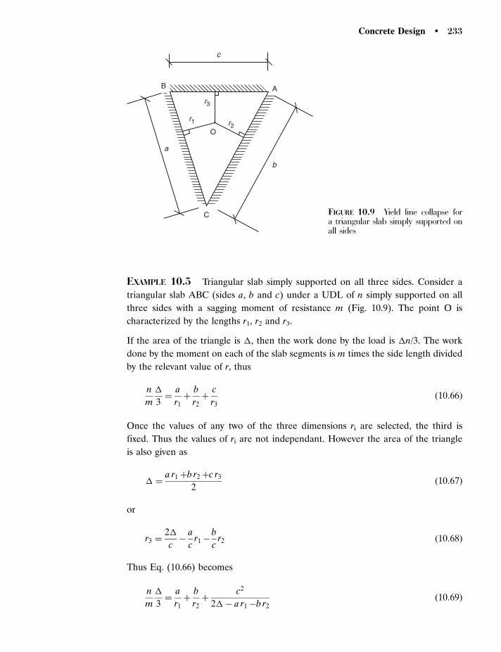
EXAMPLE 10.5 Triangular slab simply supported on all three sides. Consider a
triangular slab ABC (sides a, b and c) under a UDL of n simply supported on all
three sides with a sagging moment of resistance m (Fig. 10.9). The point O is
characterized by the lengths r1, r2 and r3.
If the area of the triangle is �, then the work done by the load is �n/3. The work
done by the moment on each of the slab segments is m times the side length divided
by the relevant value of r, thus
n
m
�
3¼
a
r1þ
b
r2þ
c
r3ð10:66Þ
Once the values of any two of the three dimensions ri are selected, the third is
fixed. Thus the values of ri are not independant. However the area of the triangle
is also given as
� ¼a r1 þb r2 þc r3
2ð10:67Þ
or
r3 ¼2�
c�a
cr1 �
b
cr2 ð10:68Þ
Thus Eq. (10.66) becomes
n
m
�
3¼
a
r1þ
b
r2þ
c2
2�� a r1 �b r2ð10:69Þ
B A
C
O
b
c
a
r1
r3
r2
FIGURE 10.9 Yield line collapse fora triangular slab simply supported onall sides
Concrete Design � 233
Equation (10.69) needs to be partially differentiated with respect to r1 and r2, thus
�a
r21
�ð�aÞ c2
ð2�� a r1 �b r2 Þ2¼ 0 ð10:70Þ
or
1
r21
¼c2
ð2�� a r1 �b r2 Þ2
ð10:71Þ
and, similarly
�b
r22
�ð�bÞ c2
ð2�� a r1 �b r2 Þ2¼ 0 ð10:72Þ
or
1
r22
¼c2
ð2�� a r1 �b r2 Þ2
ð10:73Þ
The right-hand sides of Eqs (10.71) and (10.73) are identical, thus
r1 ¼ r2 ¼ r ð10:74Þ
From either Eq. (10.71) or (10.73),
1
r2¼
c2
ð2�� ar � br Þ2ð10:75Þ
or
cr ¼ 2�� ar � br ð10:76Þ
or from Eq. (10.68),
r3 ¼ r ð10:77Þ
Thus, the point O is the centre of the inscribed circle of the triangle. Thus
n
3m
ðaþ bþ cÞr
2¼
aþ bþ c
rð10:78Þ
or
n ¼6m
r2ð10:79Þ
To determine r it should be noted that the area of a triangle � is given by
� ¼ffiffiffiffiffiffiffiffiffiffiffiffiffiffiffiffiffiffiffiffiffiffiffiffiffiffiffiffiffiffiffiffiffiffiffiffiffiffiffiffiffiffiffisðs� aÞ ðs� bÞ ðs� cÞ
p¼ sr ð10:80Þ
234 � Chapter 10 / Reinforced Concrete Slabs
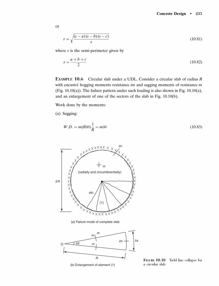
or
r ¼
ffiffiffiffiffiffiffiffiffiffiffiffiffiffiffiffiffiffiffiffiffiffiffiffiffiffiffiffiffiffiffiffiffiffiffiffiffiffiffiffiffiffiðs� aÞ ðs� bÞ ðs� cÞ
s
rð10:81Þ
where s is the semi-perimeter given by
s ¼aþ bþ c
2ð10:82Þ
EXAMPLE 10.6 Circular slab under a UDL. Consider a circular slab of radius R
with encastre hogging moments resistance im and sagging moments of resistance m
(Fig. 10.10(a)). The failure pattern under such loading is also shown in Fig. 10.10(a),
and an enlargement of one of the sectors of the slab in Fig. 10.10(b).
Work done by the moments:
(a) Sagging:
W :D: ¼ mðR��Þ1
R¼ m�� ð10:83Þ
m
etc.
O
R
mm
mim δs
δq
2R
(radially and circumferentially)
(a) Failure mode of complete slab
(b) Enlargement of element (1)
(1)
im
FIGURE 10.10 Yield line collapse fora circular slab
Concrete Design � 235
(b) Hogging:
W :D: ¼ imðR��Þ1
R¼ im�� ð10:84Þ
From Eqs (10.83) and (10.84) the total work done by the moments is
W :D: ¼ m�� þ im�� ¼ ð1 þ iÞm�� ð10:85Þ
Work done by loads:
The sector of a circle may be treated as a triangle as �� is small.
W :D: ¼1
3n
1
2R
2 ��
� �¼
nR2 ��
6ð10:86Þ
Equating Work done from Eqs (10.85) and (10.86) gives
m ¼nR2
6ð1 þ iÞð10:87Þ
EXAMPLE 10.7 Circular slab with a central point load P. Total Work done by the
moments is obtained by summing the incremental work done over a single sector
given by Eq. (10.85) over the whole slab
W :D: ¼X
mð1 þ iÞ�� ¼ 2 mð1 þ iÞ ð10:88Þ
Work done by load:
W :D: ¼ P� 1 ð10:89Þ
Equating work done from Eqs (10.88) and (10.89) gives
m ¼P
2 ð1 þ iÞð10:90Þ
It should be noted that the moment of resistance for a point load on a circular slab is
independent of the radius of the slab. This has the implication that a possible
collapse mechanism for a single point load on any shape slab is circular with the
radius such that the circle just touches the nearest point of the slab to the load.
Yield lines comprising circular portions occur in a number of possible instances,
namely situations where the yield criterion may be violated with straight yield lines,
around point supports (or columns) and under any instances of point loads.
236 � Chapter 10 / Reinforced Concrete Slabs

EXAMPLE 10.8 Point load at the corner of a cantilever slab (Fig. 10.11). The
overall collapse mechanism involving a hogging yield line at the encastre support
must be checked. This needs only simple statics and will not be considered further.
There are two further collapse mechanisms that must be considered.
The first is a straight yield line which requires top or hogging steel (Fig. 10.11(b)).
W.D. by moments:
W :D: ¼ imffiffiffi2
p�L
ffiffiffi2
p
�L¼ 2im ð10:91Þ
P
45°
CL
bLA
A
4 2
f
p f−
4 2
p f−
Corner A
(a) Basic layout
(b) Corner yield line
(c) Part fan
im
m
hogging
sagging
FIGURE 10.11 Yield line collapsefor a point load at the corner of acantilever slab
Concrete Design � 237
W.D. by loads:
W :D: ¼ P� 1 ð10:92Þ
So equating work done from Eqs (10.91) and (10.92) gives
m ¼P
2ið10:93Þ
An alternative pattern is where the yield line is in part circular and in part two
straight lines (Fig. 10.11(c)). Note a complete quarter circle cannot occur as this
would imply a moment could be generated normal to a free edge.
The work equation can be written as
P ¼ ð1 þ iÞm�þ 2im tan
4��
2
� �ð10:94Þ
Differentiating Eq. (10.94) with respect to � gives
� ¼1ffiffii
p ð10:95Þ
or, substituting Eq. (10.95) into Eq. (10.94) gives
m ¼P
ðiþ 1Þ ð =2Þ � 2 arctanð1=ffiffii
pÞ
�þ ð2=
ffiffii
pÞ
ð10:96Þ
Note that if the sagging and hogging yield moments are equal (i¼ 1), then the
second mechanism cannot form and reduces to the straight line mechanism above.
With the above mechanisms in mind, and the fact that the classical straight line
solution for the square slab can be shown to violate the yield criterion at the corners,
alternative mechanisms can be suggested.
EXAMPLE 10.9 Alternative approaches for a square slab. There are two possible
additional mechanisms for the failure of a square slab. To keep the algebra
reasonably simple, the hogging and sagging yield lines have equal moments of
resistance m, i.e. i¼ 1. The classic solutions for equal hogging and sagging
reinforcement are for a uniformly distributed load n, m¼ nL2/48, and for a central
point load P, m¼P/16.
The first solution involves partial collapse with straight lines leaving the corners
intact (known as corner levers), and the second involves fans.
Mechanism 1 (UDL):
This is illustrated in Fig. 10.12(a). Only one quarter of the slab need be considered.
First a little geometry:
XY ¼ffiffiffi2
px ð10:97Þ
238 � Chapter 10 / Reinforced Concrete Slabs
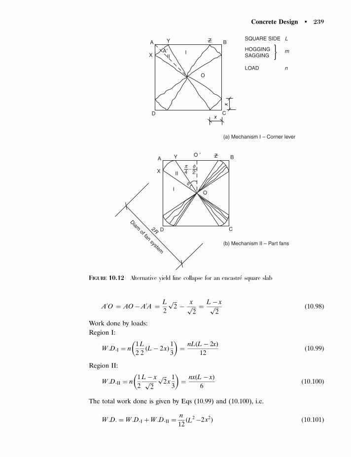
A0O ¼ AO� A0A ¼L
2
ffiffiffi2
p�
xffiffiffi2
p ¼L� xffiffiffi
2p ð10:98Þ
Work done by loads:
Region I:
W :D:I ¼ n1
2
L
2ðL� 2 xÞ
1
3
� �¼
nLðL� 2xÞ
12ð10:99Þ
Region II:
W :D:II ¼ n1
2
L� xffiffiffi2
pffiffiffi2
px
1
3
� �¼
nxðL� xÞ
6ð10:100Þ
The total work done is given by Eqs (10.99) and (10.100), i.e.
W :D: ¼ W :D:I þW :D:II ¼n
12ðL
2 �2 x2Þ ð10:101Þ
A
A′X
Y Z B
O
III
D
A
X
Y B
OI
4 2IIp − f
f
D2R
Diam of fan system
C
ZO ′
C
(a) Mechanism I – Corner lever
SQUARE SIDE L
LOAD
m
n
HOGGINGSAGGING
(b) Mechanism II – Part fans
x
x
FIGURE 10.12 Alternative yield line collapse for an encastre square slab
Concrete Design � 239
Work done by moments:
Region I:
W :D:I ¼ ðmþmÞðL� 2 xÞ1
L=2¼ 4m
L� 2 x
Lð10:102Þ
Region II:
W :D:II ¼ ðmþmÞffiffiffi2
px
1
ðL� xÞ=ffiffiffi2
p ¼ 4mx
L� xð10:103Þ
Total work done is given by Eqs (10.102) and (10.103), i.e.
W :D: ¼ W :D:I þW :D:II ¼4m
L
L2 � 2 xLþ 2 x2
L� xð10:104Þ
Equating work done by the loads from Eq. (10.101) and moments from Eq. (10.104)
gives
nL
48m¼
L2 � 2 xLþ 2 x2
ðL� xÞ ðL2 � 2 x2Þð10:105Þ
Differentiate the right-hand side of Eq. (10.105) with respect to x,
L2 � 2 xLþ 2 x2
ðL� xÞ ðL2 � 2 x2Þ¼
4x� 2L
ðL� xÞð�4xÞ þ ðL2 � 2 x2Þð�1Þ
¼4x� 2L
6 x2 � 4xL� L2ð10:106Þ
or, simplifying
4 x4 � 8L x3 þ 12L2 x2 � 8L3xþ L4 ¼ 0 ð10:107Þ
Solving Eq. (10.107) gives x/L¼ 0,1594; 0,8576; 0,5182� 1,249i.
The last three roots are inadmissible either because they are outside the limits of
0� x� 0,5 or are complex. The only acceptable solution is x/L¼ 0,1594.
Substituting this value into Eq. (10.105) gives
m ¼nL2
48 � 0,917¼
nL2
44,02ð10:108Þ
i.e. 9 per cent more reinforcement is required over the traditional solution.
Mechanism II:
This is illustrated in Fig. 10.12(b). Again only one quarter of the slab need be
considered.
240 � Chapter 10 / Reinforced Concrete Slabs

Again a little geometry:
YZ ¼ 2O0Y ¼ 2L
2tan
4��
2
� �¼ L tan
4��
2
� �ð10:109Þ
R ¼L
2 cos½ð =4Þ � ð�=2Þ�ð10:110Þ
The fans are treated as if each contained a large number of sectors subtending
small angles at the centroid with each incremental sector displacing by 1/3 (as
in the complete circular collapse).
Work done by loads:
Region I:
W :D:I ¼ n1
2
L
2L tan
4��
2
� �1
3
� �
¼nL2
12tan
4��
2
� �ð10:111Þ
Region II:
W :D:II ¼ nR2
2�
1
3
� �¼
nL2
12
�=2
cos2 ð =4Þ � ð�=2Þ½ �ð10:112Þ
The total work done is given by Eqs (10.111) and (10.112), i.e.
W :D: ¼ W :D:I þW :D:II
¼nL2
12
�=2
cos2 ð =4Þ � ð�=2Þ½ �þ tan
4��
2
� �� �ð10:113Þ
Work done by moments:
Region I:
W :D:I ¼ ðmþmÞL tan
4��
2
� �1
L=2¼ 4m tan
4��
2
� �ð10:114Þ
Region II:
W :D:II ¼ ðmþmÞ� ð10:115Þ
Total work done is given by Eqs (10.114) and (10.115), i.e.
W :D: ¼ W :D:I þW :D:II ¼ 4m�
2þ tan
4��
2
� �� �ð10:116Þ
Concrete Design � 241
Equating work done by the loads from Eq. (10.113) and moments from Eq. (10.116)
gives
nL2
48m¼
ð�=2Þ þ tan ð =4Þ � ð�=2Þ½ �
ð�=2Þ= cos2 ð =4Þ � ð�=2Þ½ � þ tan ð =4Þ � ð�=2Þ½ �ð10:117Þ
The RHS of Eq. (10.117) was optimized using a spread-sheet to give a value of
0,9055 with �¼ 0,488 rad (288) thus from Eq. (10.117),
m ¼nL2
48 � 0,9055¼
nL2
43,46ð10:118Þ
i.e. 10 per cent more reinforcement is required over the traditional solution.
Thus, it is observed that the classical straight yield line pattern overestimates the
carrying capacity of a square slab by around 10 per cent. In practice this error may
not be significant as detailing generally overprovides reinforcement (and must not
underprovide!). It does however indicate that care needs to be taken. It is also to be
noted that the correct solution is greater than either the straight yield line or the
case when the circular yield line forms the complete pattern, i.e. when ’¼ /2 and
R¼L/2. In the latter case,
m ¼nR2
6ðiþ 1Þ¼
n ðL=2Þ½ �2
6ð1 þ 1Þ¼
nL2
48ð10:119Þ
EXAMPLE 10.10 Central Point load, P. The mechanisms take exactly the same
form as in Example 10.9, hence the work done by the moments is unchanged.
In both mechanisms I and II, for one quarter of the slab, the work done by the
load is (P/4)�1.
Mechanism I:
The work done by the moments is given by Eq. (10.104), thus the complete work
equation may be written as
P
4¼
4m
L
L2 � 2 xLþ 2 x2
L� xð10:120Þ
or
PL
16m¼
L2 � 2 xLþ 2 x2
L� xð10:121Þ
Differentiate the right-hand side of Eq. (10.121) with respect to x to give
L2 � 2 xLþ 2 x2
L� x¼
4x� 2L
�1¼ 2L� 4x ð10:122Þ
242 � Chapter 10 / Reinforced Concrete Slabs

Simplifying gives
2 x2 � 4xLþ L2 ¼ 0 ð10:123Þ
or
x ¼Lffiffiffi
2p
ffiffiffi2
p� 1
� �ð10:124Þ
Back-substituting gives
m ¼P
32ffiffiffi2
p� 1
� ¼ P
13,25ð10:125Þ
This is around 17 per cent lower than the classical solution.
Mechanism II:
The work done by the moments is given by Eq. (10.116), thus the complete work
equation is given by
P
4¼ 4m
�
2þ tan
4��
2
� �� �ð10:126Þ
or
P
16m¼�
2þ tan
4��
2
� �ð10:127Þ
Differentiate the right-hand side of Eq. (10.127) with respect to � to give
1
2þ
�1
2
� �1
cos2 ð =4Þ � ð�=2Þ½ �¼ 0 ð10:128Þ
This gives �¼ /2, i.e. the fan becomes a complete circle with m given by
m ¼P
4 ¼
P
12,57ð10:129Þ
and is around 21 per cent lower than the classical solution. The results are
summarized in Table 10.1 for both the UDL and point load.
In conclusion, it may be observed that from the complete set of results substantially
larger errors are produced by not considering fans (or alternative straight line
patterns) for loading due to point loads (or column reactions) than for uniformly
distributed loads.
Concrete Design � 243

EXAMPLE 10.11 Slabs on column supports. Consider a square slab supported at
its corners by columns carrying a UDL (Fig. 10.13(a)).
Mechanism I:
The immediate response for a simple solution to the problem is to adopt that is
shown in Fig. 10.13(b). It can be readily shown that this gives
m ¼nL2
8ð10:130Þ
Mechanism II:
A possible alternative is that shown in Fig. 10.13(c) with diagonal yield lines. The
virtual work equation for this case may be written as,
4mðffiffiffi2
p�LÞ
ffiffiffi2
p
�L
!¼ n L
2 �4ð�L Þ
2
2
" #� 1 þ 4n
ð�L Þ2
2�
2
3ð10:131Þ
where the first term on the right-hand side is due to the centre of the slab deflecting
by unity and the second term is due to the four corner triangles, the centres of gravity
of which deflect by 2/3.
The work equation reduces to
m ¼nL2
81 �
2 �2
3
� �ð10:132Þ
The value of m tends to a maximum when � tends to zero. This maximum value
of m is again nL2/8.
An elastic solution to the problem of a slab supported on corner columns indicates
that there will be hogging and twisting moments over the columns. Neither yield
solution gives any indication of the existence of any such moments, nor any
mobilization of any top steel. It is thus necessary to consider the possibility of the
formation of fans. Although it has already been demonstrated that a complete
quarter circle yield line pattern cannot physically occur (Example 10.8), for this
exercise it will be assumed possible (Fig. 10.13(d)). It should also be noted that if this
TABLE 10.1 Comparison of failure moments of square slabs.
Type of failure UDL % Error Point load % Error
Classical 1/48 � 1/16 �
Corner lever 1/44,02 9 1/13,25 21Part Fans 1/43,46 10 1/12,57 27Complete circle 1/48 � 1/12,57 27
�nL2�P
Note: The percentage error is determined using the classical solution as the basis.
244 � Chapter 10 / Reinforced Concrete Slabs

slab were part of a multi-bay flat slab, circular yield lines around the column would
be possible, and would need considering.
The centroid of a quarter circle is at a distance of 4ffiffiffi2
pR=3 from the centre. Thus,
if the perimeter of the quarter circle undergoes a virtual displacement of unity,
the centroid is displaced by ð1=RÞ � ð4ffiffiffi2
pR=3 Þ ¼ 4
ffiffiffi2
p=3 . Thus, the equilibrium
equation can be written as,
2mð1 þ iÞ R1
R
� �¼ nðL
2 � R2Þ � 1 þ n R
2 4ffiffiffi2
p
3
!ð10:133Þ
Square slab of side
(a) Slab details
Radius R
(b) Mode 1
45°
45°
45°
(d) Mode 3
(c) Mode 2
(e) Mode 4(all corners identical)
Part circular fanRadius R, angle
L
L/2
bL
p / 2 − 2f
L/2
m
f
FIGURE 10.13 Collapse mechanisms for a square slab on corner columns
Concrete Design � 245
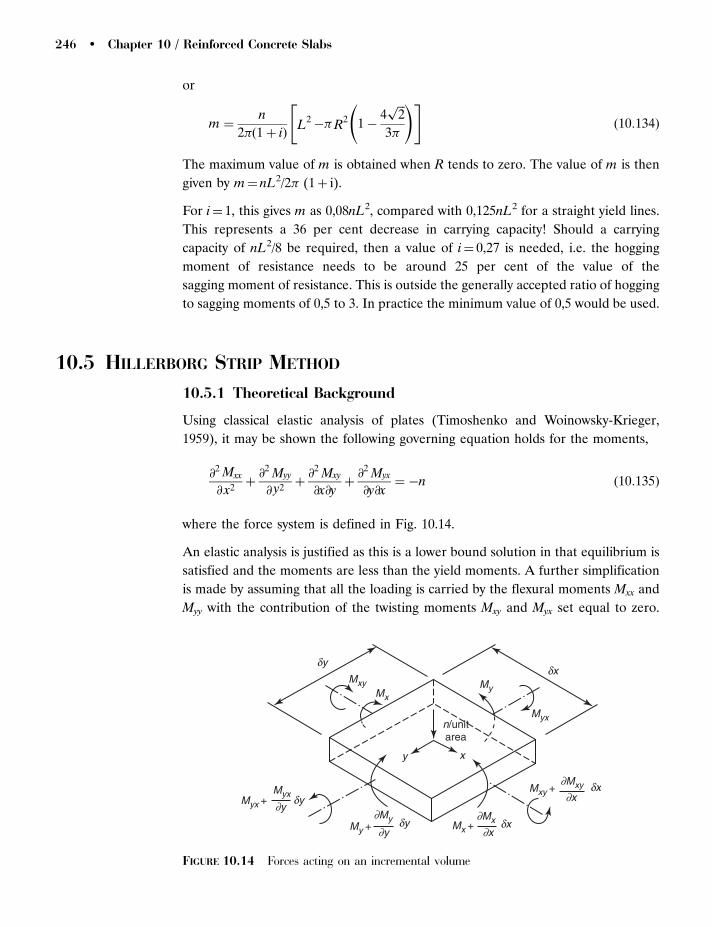
or
m ¼n
2 ð1 þ iÞL
2 � R2 1 �
4ffiffiffi2
p
3
!" #ð10:134Þ
The maximum value of m is obtained when R tends to zero. The value of m is then
given by m¼ nL2/2 (1þ i).
For i¼ 1, this gives m as 0,08nL2, compared with 0,125nL2 for a straight yield lines.
This represents a 36 per cent decrease in carrying capacity! Should a carrying
capacity of nL2/8 be required, then a value of i¼ 0,27 is needed, i.e. the hogging
moment of resistance needs to be around 25 per cent of the value of the
sagging moment of resistance. This is outside the generally accepted ratio of hogging
to sagging moments of 0,5 to 3. In practice the minimum value of 0,5 would be used.
10.5 HILLERBORG STRIP METHOD
10.5.1 Theoretical Background
Using classical elastic analysis of plates (Timoshenko and Woinowsky-Krieger,
1959), it may be shown the following governing equation holds for the moments,
@2 Mxx
@ x2þ@2 Myy
@ y2þ@2 Mxy
@x@yþ@2 Myx
@y@x¼ �n ð10:135Þ
where the force system is defined in Fig. 10.14.
An elastic analysis is justified as this is a lower bound solution in that equilibrium is
satisfied and the moments are less than the yield moments. A further simplification
is made by assuming that all the loading is carried by the flexural moments Mxx and
Myy with the contribution of the twisting moments Mxy and Myx set equal to zero.
dy
dy
dy∂y
∂y ∂x
∂My ∂Mx
∂x
∂Mxy dx
dx
dx
y
MxyMx
n/unitarea
Myx
My
Mxy +
Mx +
Myx +Myx
My +
x
FIGURE 10.14 Forces acting on an incremental volume
246 � Chapter 10 / Reinforced Concrete Slabs

Thus Eq. (10.135) becomes
@2 Mxx
@ x2þ@2 Myy
@ y2¼ �n ð10:136Þ
The load n may be considered to be partially resisted by xx axis flexure and partially
by yy axis flexure with a distribution coefficient � introduced such that
@2 Mxx
@ x2¼ ��n ð10:137Þ
and
@2 Myy
@ y2¼ �ð1 � �Þn ð10:138Þ
Equations (10.137) and (10.138) will be recognized as the equations governing
flexure of simple beam elements. Thus, a numerical approach to utilizing elastic
plate bending theory can be set up by dividing the slab into a series of strips in the
x and y directions and distributing the loading between these strips. It is normal
practice to use only two values of �, namely zero or unity with the resultant load
distribution being in either the x or the y directions. The exact pattern of load
distribution is at the designer’s discretion but clearly it is more economic to allow the
majority of the loading where possible to be taken on the shorter span. At slab
corners it is generally acceptable to use load dispersion lines at 458. The number of
load carrying strips should not be excessive as this may produce detailing problems
with continually changing bar spacing. Too small a number however will lead to
inefficient use of reinforcement. For background information on the Hillerborg Strip
Method and for advanced applications, reference should be made to Wood and
Armer (1968). Note the Hillerborg Strip Method does not impose compatibility of
deformations between individual strips.
EXAMPLE 10.12 Application of Hillerborg Strip Method. Consider the simply
supported rectangular slab shown in Fig. 10.15, taking load distribution lines at
458 from the corners. Fig. 10.15(b) shows a possible distribution of load carrying
strips.
Strip 1 (Fig. 10.15(c)):
The whole slab is under a UDL of n, hence
mSd,1 ¼nL2
y
8ð10:139Þ
Strip 2 (Fig. 10.15(d)):
The loading here comprises two triangular shaped load patches at the ends of the
slab. From Moy (1996), it may be shown that for this case
mRSd ¼ KnðL1 þ L2Þ
2
8ð10:140Þ
Concrete Design � 247

where in the general case (Fig. 10.15(e)) K is given by
K ¼4
31 �
1
2 þ ðL1=L2Þ þ ðL2=L1Þ
� �ð10:141Þ
Strip 3 (Fig. 10.15(f)):
This can be treated in a similar fashion to Strip 2.
Ly
Lx
(a) Slab geometryLoad dispersionlines
indicatesdirection inwhich loadspans
(b) Loaddispersion
Strip 1
Strip 3 Strip 3
Strip 2
Strip
(c) Strip 1 (d) Strip 2
(f) Strip 3
(e) Definition of L1 and L2
Lx / 2
Lx
L1
L1
L2
L2
Lx / 2
Lx / 2
Ly − Lx
2
45°
45°
Loadedarea
FIGURE 10.15 Hillerborg Strip Method
248 � Chapter 10 / Reinforced Concrete Slabs

10.6 SLAB DESIGN AND DETAILING
10.6.1. Ratio of Hogging and Sagging Moments of Resistance
The ratio of hogging to sagging moments of resistance i may according to cl 5.6.2 (2)
be taken between values of 0,5 and 2,0. It is suggested however that to avoid
problems with the serviceability limit states of deflection and cracking that the likely
distribution of moments corresponding to an elastic analysis be borne in mind and
that the value of i be taken between 1 and 2.
10.6.2 Design Considerations
The maximum value of xu/d should be 0,25 for concretes of strengths less than or
equal to C50, above C50 the limit is 0,15 (cl 5.6.2 (2)).
10.6.3 Detailing Requirements
In general these are the same as beams except that:
(1) The maximum spacing of bars smax,slabs is for the main reinforcement
3h� 400 mm (cl 9.3.1.1 (3)), and for secondary reinforcement 3,5h� 450 mm.
Provided these rules are complied with and h� 200 mm further measures (or
checks) on crack widths need not be made (cl 7.3.3 (1)).
(2) At least half the sagging reinforcement should continue to the support and
be fully anchored (cl 9.3.1.2 (1)). Where the slab has partial fixity not taken
into account in the analysis, then the hogging reinforcement should be
capable of resisting at least 25 per cent of the maximum moment in the
adjacent span and should extend for a length of 0,2 times the adjacent span
(cl 9.3.1.2 (2)).
(3) At a free edge, reinforcement should be detailed as in Fig. 10.16 to allow correct
placement and to resist any implicit twisting moments.
(4) Curtailment. This is in accordance with beams. Where, however, a full fire safety
engineering approach is adopted; it will be necessary to check the anchorage
Full tensionlap
Slab
'U' bar Mainreinforcement
FIGURE 10.16 Edge reinforcementfor torsion
Concrete Design � 249
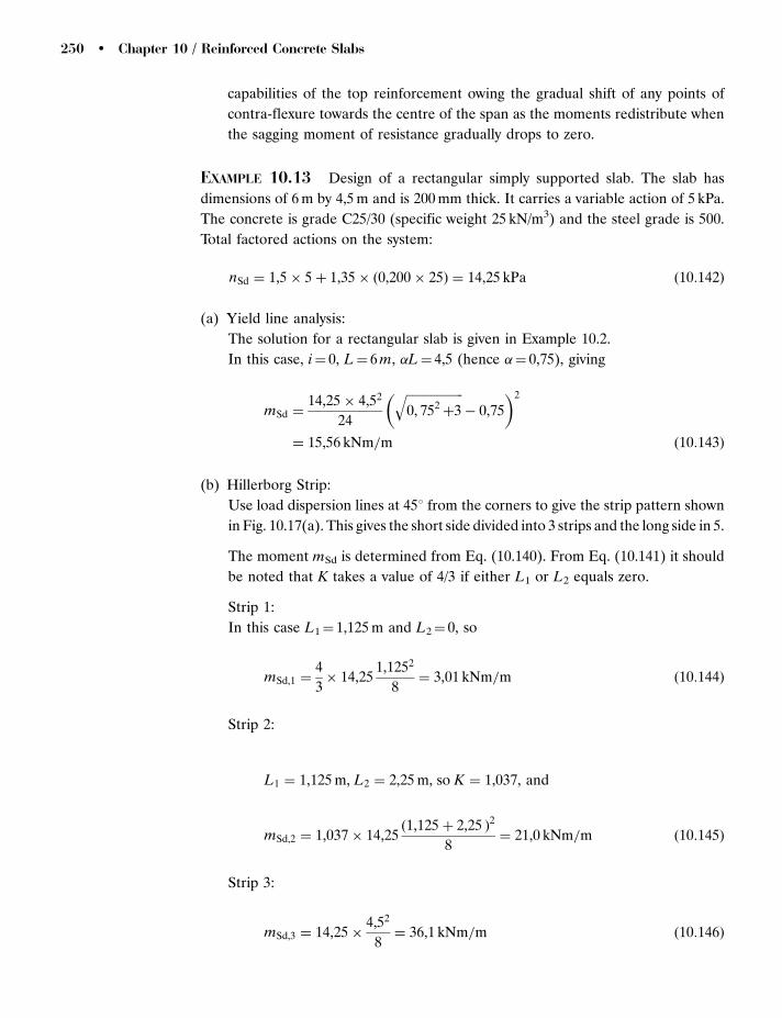
capabilities of the top reinforcement owing the gradual shift of any points of
contra-flexure towards the centre of the span as the moments redistribute when
the sagging moment of resistance gradually drops to zero.
EXAMPLE 10.13 Design of a rectangular simply supported slab. The slab has
dimensions of 6 m by 4,5 m and is 200 mm thick. It carries a variable action of 5 kPa.
The concrete is grade C25/30 (specific weight 25 kN/m3) and the steel grade is 500.
Total factored actions on the system:
nSd ¼ 1,5 � 5 þ 1,35 � ð0,200 � 25Þ ¼ 14,25 kPa ð10:142Þ
(a) Yield line analysis:
The solution for a rectangular slab is given in Example 10.2.
In this case, i¼ 0, L¼ 6m, �L¼ 4,5 (hence �¼ 0,75), giving
mSd ¼14,25 � 4,52
24
ffiffiffiffiffiffiffiffiffiffiffiffiffiffiffiffiffiffiffi0, 752
þ3
q� 0,75
� �2
¼ 15,56 kNm=m ð10:143Þ
(b) Hillerborg Strip:
Use load dispersion lines at 458 from the corners to give the strip pattern shown
in Fig. 10.17(a). This gives the short side divided into 3 strips and the long side in 5.
The moment mSd is determined from Eq. (10.140). From Eq. (10.141) it should
be noted that K takes a value of 4/3 if either L1 or L2 equals zero.
Strip 1:
In this case L1¼ 1,125 m and L2¼ 0, so
mSd,1 ¼4
3� 14,25
1,1252
8¼ 3,01 kNm=m ð10:144Þ
Strip 2:
L1 ¼ 1,125 m, L2 ¼ 2,25 m, so K ¼ 1,037, and
mSd,2 ¼ 1,037 � 14,25ð1,125 þ 2,25 Þ2
8¼ 21,0 kNm=m ð10:145Þ
Strip 3:
mSd,3 ¼ 14,25 �4,52
8¼ 36,1 kNm=m ð10:146Þ
250 � Chapter 10 / Reinforced Concrete Slabs

Strip 4:
L1 ¼ 0, L2 ¼ 1,5 m, K ¼ 4=3
mSd,4 ¼4
3� 14,25
1,52
8¼ 5,34 kNm=m ð10:147Þ
Strip 5:
In order to calculate K it should be noted that the strip is that symmetric about
its centre line, thus
L1 ¼ 2,25 m, L2 ¼ 1,50, K ¼ 1,013:
mSd,4 ¼ 1,013 � 14,25ð1,5 þ 2,25 Þ2
8¼ 25,4 kNm=m ð10:148Þ
Strip1
Strip2
Strip3
Strip2
Strip1
Strip 4
4.5
1.5
1.5
1.5
1.51.125 1.125 1.125
1.125
1.125 2.250 2.250
1.5
1.5
1.501.50
1.501.50 3.00
2.25 1.50 2.25
2.2501.1251.
125
1.125
1.125
6.0
45°
45°
Strip 5
Strip 4
(a) Strip details
(b) Strip 1
(d)Strip 4
(e)Strip 5
(c) Strip 2
FIGURE 10.17 Hillerborg Strip approach
Concrete Design � 251

Design of flexural reinforcement:
Assume cover to be 20 mm, and D12 bars, thus the mean effective depth for both
directions is d¼ 200� 20� 12¼ 168 mm.
Strictly d should be calculated for each direction, however using a mean value will
not induce significant errors.
(a) Yield line:
mSd ¼ 15,56 kNm=m
M=bd2fck ¼ 15,564 � 106=ð1000 � 1682 � 25Þ ¼ 0,0221
From Eq. (6.22)
As fyk=dbfck ¼ 0,652 �ffiffiffiffiffiffiffiffiffiffiffiffiffiffiffiffiffiffiffiffiffiffiffiffiffiffiffiffiffiffiffiffiffiffiffiffiffiffiffiffiffiffiffiffiffi0,425 � ð1,5M=bd2fckÞ
p¼ 0,026
xu=d ¼ 1,918As fyk=dbfck ¼ 1,918 � 0,026 ¼ 0,055 0,25
As ¼ 0,026 � 1000 � 168 � 25=500 ¼ 218 mm2=m:
Minimum longitudinal steel:
The greater of 0,0013btd or 0,26fctmbtd/fyk where bt is the mean width of the
tension zone (cl 9.2.1.1 (1)).
Calculation of As,min:
0,0013btd ¼ 0,0013 � 1000 � 168 ¼ 218 mm2=m:
fctm ¼ 0,3f ð2=3Þck ¼ 0,3 � 25ð2=3Þ ¼ 2,56 MPa
0,26fctmbtd=fyk ¼ 0,26 � 2,56 � 1000 � 168=500 ¼ 224 mm2
Actual required is less than As,min. Maximum spacing is lesser of 3 h or 400 mm.
Critical value is 400 mm.
Deflection check:
¼ 0,001ffiffiffiffiffifck
p¼ 0,001
ffiffiffiffiffi25
p¼ 5,0 � 10�3
¼ As=bd ¼ 262=ð1000 � 168Þ ¼ 1,56 � 10�3. Thus 5 0
Thus allowable l/d is given by
l
d¼ K 11 þ 1,5
ffiffiffiffiffifck
p 0
þ 3,2
ffiffiffiffiffifck
p 0
� 1
� �3=2" #
or
l
d¼ 1,0 11 þ 1,5
ffiffiffiffiffi25
p 0,00500
0,00156þ 3,2
ffiffiffiffiffi25
p 0,00500
0,00156� 1
� �3=2" #
¼ 87:43
252 � Chapter 10 / Reinforced Concrete Slabs
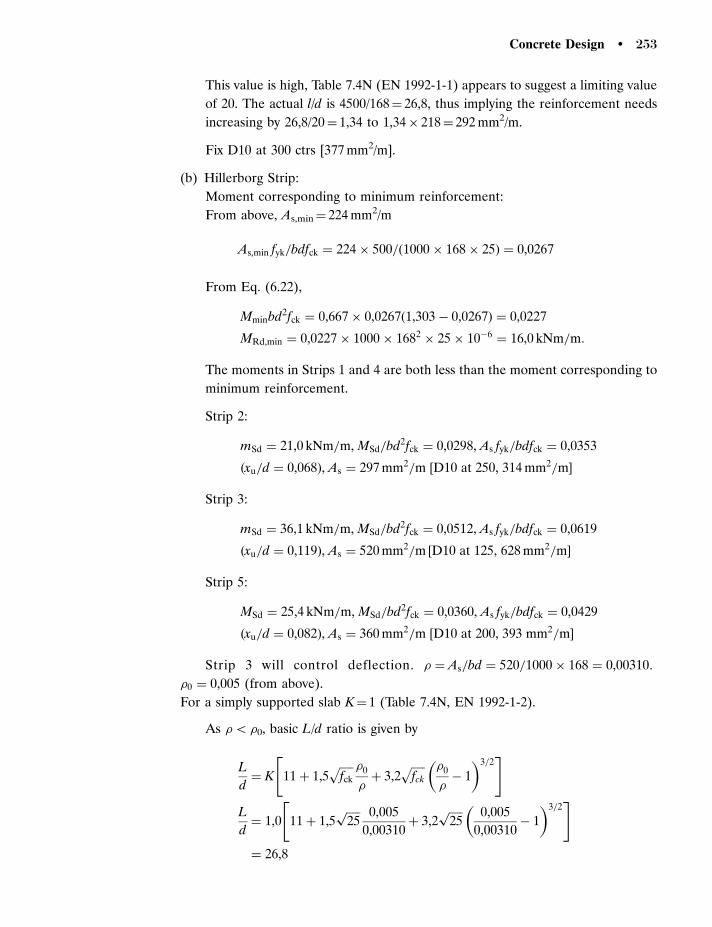
This value is high, Table 7.4N (EN 1992-1-1) appears to suggest a limiting value
of 20. The actual l/d is 4500/168¼ 26,8, thus implying the reinforcement needs
increasing by 26,8/20¼ 1,34 to 1,34� 218¼ 292 mm2/m.
Fix D10 at 300 ctrs [377 mm2/m].
(b) Hillerborg Strip:
Moment corresponding to minimum reinforcement:
From above, As,min¼ 224 mm2/m
As,min fyk=bdfck ¼ 224 � 500=ð1000 � 168 � 25Þ ¼ 0,0267
From Eq. (6.22),
Mminbd2fck ¼ 0,667 � 0,0267ð1,303 � 0,0267Þ ¼ 0,0227
MRd,min ¼ 0,0227 � 1000 � 1682 � 25 � 10�6 ¼ 16,0 kNm=m:
The moments in Strips 1 and 4 are both less than the moment corresponding to
minimum reinforcement.
Strip 2:
mSd ¼ 21,0 kNm=m, MSd=bd2fck ¼ 0,0298, As fyk=bdfck ¼ 0,0353
ðxu=d ¼ 0,068Þ, As ¼ 297 mm2=m ½D10 at 250, 314 mm2=m�
Strip 3:
mSd ¼ 36,1 kNm=m, MSd=bd2fck ¼ 0,0512, As fyk=bdfck ¼ 0,0619
ðxu=d ¼ 0,119Þ, As ¼ 520 mm2=m ½D10 at 125, 628 mm2=m�
Strip 5:
MSd ¼ 25,4 kNm=m, MSd=bd2fck ¼ 0,0360, As fyk=bdfck ¼ 0,0429
ðxu=d ¼ 0,082Þ, As ¼ 360 mm2=m ½D10 at 200, 393 mm2=m�
Strip 3 will control deflection. ¼ As=bd ¼ 520=1000 � 168 ¼ 0,00310:
0 ¼ 0,005 (from above).
For a simply supported slab K¼ 1 (Table 7.4N, EN 1992-1-2).
As 5 0, basic L/d ratio is given by
L
d¼ K 11 þ 1,5
ffiffiffiffiffifck
p 0
þ 3,2
ffiffiffiffiffifck
p 0
� 1
� �3=2" #
L
d¼ 1,0 11 þ 1,5
ffiffiffiffiffi25
p 0,005
0,00310þ 3,2
ffiffiffiffiffi25
p 0,005
0,00310� 1
� �3=2" #
¼ 26,8
Concrete Design � 253
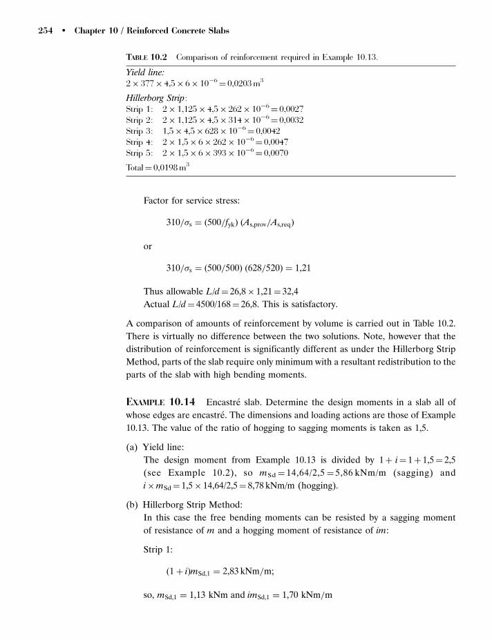
Factor for service stress:
310=s ¼ ð500=fykÞ ðAs,prov=As,reqÞ
or
310=s ¼ ð500=500Þ ð628=520Þ ¼ 1,21
Thus allowable L/d¼ 26,8� 1,21¼ 32,4
Actual L/d¼ 4500/168¼ 26,8. This is satisfactory.
A comparison of amounts of reinforcement by volume is carried out in Table 10.2.
There is virtually no difference between the two solutions. Note, however that the
distribution of reinforcement is significantly different as under the Hillerborg Strip
Method, parts of the slab require only minimum with a resultant redistribution to the
parts of the slab with high bending moments.
EXAMPLE 10.14 Encastre slab. Determine the design moments in a slab all of
whose edges are encastre. The dimensions and loading actions are those of Example
10.13. The value of the ratio of hogging to sagging moments is taken as 1,5.
(a) Yield line:
The design moment from Example 10.13 is divided by 1þ i¼ 1þ 1,5¼ 2,5
(see Example 10.2), so mSd ¼ 14,64/2,5 ¼ 5,86 kNm/m (sagging) and
i�mSd¼ 1,5� 14,64/2,5¼ 8,78 kNm/m (hogging).
(b) Hillerborg Strip Method:
In this case the free bending moments can be resisted by a sagging moment
of resistance of m and a hogging moment of resistance of im:
Strip 1:
ð1 þ iÞmSd,1 ¼ 2,83 kNm=m;
so, mSd,1 ¼ 1,13 kNm and imSd,1 ¼ 1,70 kNm=m
TABLE 10.2 Comparison of reinforcement required in Example 10.13.
Yield line:2� 377� 4,5� 6� 10�6
¼ 0,0203m3
Hillerborg Strip:Strip 1: 2� 1,125� 4,5� 262� 10�6
¼ 0,0027Strip 2: 2� 1,125� 4,5� 314� 10�6
¼ 0,0032Strip 3: 1,5� 4,5� 628� 10�6
¼ 0,0042Strip 4: 2� 1,5� 6� 262� 10�6
¼ 0,0047Strip 5: 2� 1,5� 6� 393� 10�6
¼ 0,0070
Total¼ 0,0198m3
254 � Chapter 10 / Reinforced Concrete Slabs

Strip 2:
ð1 þ iÞmSd,2 ¼ 19,80 kNm=m;
so, mSd,2 ¼ 7,92 kNm=m and imSd,2 ¼ 11,88 kNm=m
Strip 3:
ð1 þ iÞmSd,3 ¼ 33,94 kNm=m;
so, mSd,3 ¼ 13,58 kNm=m and imSd,3 ¼ 20,6 kNm=m
Strip 4:
ð1 þ iÞmSd,4 ¼ 5,03 kNm=m;
so, mSd,4 ¼ 2,01 kNm=m and imSd,4 ¼ 3,02 kNm=m
Strip 5:
ð1 þ iÞmSd,5 ¼ 23,88 kNm=m;
so, mSd,5 ¼ 9,55 kNm=m and imSd,5 ¼ 14,33 kNm=m.
The reinforcement may now be designed in the usual manner.
EXAMPLE 10.15 Slab with mixed supports. A slab is restrained on one long side
and one short side, but is simply supported on the others. The remainder of the data
is as Example 10.13.
(a) Yield line:
Without proceeding through the full solution, a convenient standard solution
exists for an isotropic slab with mixed supports (Jones and Wood, 1967)
(Fig. 10.18), so mSd is given by
m ¼na2
r
24
ffiffiffiffiffiffiffiffiffiffiffiffiffiffiffiffiffiffiffiffiffi3 þ
ar
br
� �2s
�ar
br
24
35
2
ð10:149Þ
i3m
i4m
i2m
i1mm
b
a
FIGURE 10.18 Notation for Eq. (10.149)
Concrete Design � 255

where
ar ¼2affiffiffiffiffiffiffiffiffiffiffiffi
1 þ i1p
þffiffiffiffiffiffiffiffiffiffiffiffi1 þ i4
p ð10:150Þ
and
br ¼2bffiffiffiffiffiffiffiffiffiffiffiffi
1 þ i1p
þffiffiffiffiffiffiffiffiffiffiffiffi1 þ i3
p ð10:151Þ
Note that for Eq. (10.149) to be valid br/ar4 1,0.
From Eq. (10.150),
ar ¼ 2 � 4,5=ðffiffiffiffiffiffiffiffiffiffiffiffiffiffiffiffiffiffið1 þ 1,5Þ
pþ 1Þ ¼ 3,487 m
From Eq. (10.151),
br ¼ 2 � 6,0=ðffiffiffiffiffiffiffiffiffiffiffiffiffiffiffiffiffiffið1 þ 1,5Þ
pþ 1Þ ¼ 4,649 m ðbr4arÞ
ar=br ¼ 3,487=4,649 ¼ 0,75
From Eq. (10.149),
mSd ¼13,41 � 3, 4872
24
ffiffiffiffiffiffiffiffiffiffiffiffiffiffiffiffiffiffiffiffi3 þ 0, 752
q� 0,75
� �2
¼ 8,79 kNm=m ð10:152Þ
imSd ¼ 1,5 � 8,79 ¼ 13,19 kNm=m:
(b) Hillerborg Strip Method:
For each strip, the moment at one end equals zero, the moment at the other
equals im. The free bending moment in any strip is given by Eq. (10.140), thus
assuming the maximum sagging moment occurs at the centre of a strip, the
sagging moment is given by the value from Eq. (10.140) less im/2. This is not
strictly correct as, of course, the maximum sagging moment occurs at the
point of zero shear. The above assumption will produce answers for m within
5 per cent. The values of free bending moments are those in Example 10.12.
Strip 1:
Free bending moment¼ 2,83 kNm/m
so
mSd,1 þ 0,5ð1,5mSd,1Þ ¼ 2,83 ð10:153Þ
or,
mSd,1 ¼ 1,62 kNm=m and imSd,1 ¼ 2,43 kNm=m:
256 � Chapter 10 / Reinforced Concrete Slabs

Strip 2:
Free bending moment¼ 19,8 kNm/m
so
mSd,2 þ 0,5ð1,5mSd,2Þ ¼ 19,8 ð10:154Þ
or
mSd,2 ¼ 11,3 kNm=m and imSd,2 ¼ 17,0 kNm=m:
Strip 3:
Free bending moment¼ 33,94 kNm/m
so
mSd,3 þ 0,5ð1,5mSd,3Þ ¼ 33,94 ð10:155Þ
or
mSd,3 ¼ 19,4 kNm=m and imSd,3 ¼ 29,1 kNm=m:
For strip 3, the exact solution for mSd is given by
mSd ¼ nL2 iþ 2 � 2ffiffiffiffiffiffiffiffiffiffiiþ 1
p
2i2ð10:156Þ
or
mSd ¼ 13,41 � 4,52 1,5 þ 2 � 2ffiffiffiffiffiffiffiffiffiffiffiffiffiffiffi1,5 þ 1
p
2 � 1,52¼ 20,38 kNm=m ð10:157Þ
and imSd,5 ¼ 1,5 � 20,38 ¼ 30,57 kNm=m:
The approximate solutions are within 5 per cent.
Strip 4:
Free bending moment¼ 5,03 kNm/m
so
mSd,4 þ 0,5ð1,5mSd,4Þ ¼ 5,03 ð10:158Þ
or
mSd,4 ¼ 2,88 kNm=m and imSd,4 ¼ 4,31 kNm=m:
Strip 5:
Free bending moment¼ 23,9 kNm/m
so
mSd,5 þ 0,5ð1,5mSd,5Þ ¼ 23,9 ð10:159Þ
or,
mSd,5 ¼ 13,7 kNm=m and imSd,5 ¼ 20,5 kNm=m:
Concrete Design � 257
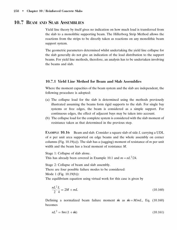
10.7 BEAM AND SLAB ASSEMBLIES
Yield line theory by itself gives no indication on how much load is transferred from
the slab to a monolithic supporting beam. The Hillerborg Strip Method allows the
reactions from the strips to be directly taken as reactions on any monolithic beam
support system.
The geometric parameters determined whilst undertaking the yield line collapse for
the slab generally do not give an indication of the load distribution to the support
beams. For yield line methods, therefore, an analysis has to be undertaken involving
the beams and slab.
10.7.1 Yield Line Method for Beam and Slab Assemblies
Where the moment capacities of the beam system and the slab are independent, the
following procedure is adopted:
(a) The collapse load for the slab is determined using the methods previously
illustrated assuming the beams form rigid supports to the slab. For single bay
systems or free edges, the beam is considered as a simple support. For
continuous edges, the effect of adjacent bays may be taken into account.
(b) The collapse load for the complete system is considered with the slab moment of
resistance taken as that determined in the previous step.
EXAMPLE 10.16 Beam and slab. Consider a square slab of side L carrying a UDL
of n per unit area supported on edge beams and the whole assembly on corner
columns (Fig. 10.19(a)). The slab has a (sagging) moment of resistance of m per unit
width and the beam has a local moment of resistance M.
Stage 1: Collapse of slab alone.
This has already been covered in Example 10.1 and m¼ nL2/24.
Stage 2: Collapse of beam and slab assembly.
There are four possible failure modes to be considered:
Mode 1 (Fig. 10.19(b)):
The equilibrium equation using virtual work for this case is given by
nL2
2
L
4¼ 2M þmL ð10:160Þ
Defining a normalized beam failure moment �mm as �mm¼M/mL, Eq. (10.160)
becomes
nL2 ¼ 8m ð1 þ �mmÞ ð10:161Þ
258 � Chapter 10 / Reinforced Concrete Slabs
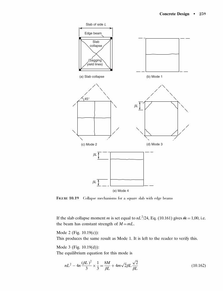
If the slab collapse moment m is set equal to nL2/24, Eq. (10.161) gives �mm¼ 1,00, i.e.
the beam has constant strength of M¼mL.
Mode 2 (Fig. 10.19(c)):
This produces the same result as Mode 1. It is left to the reader to verify this.
Mode 3 (Fig. 10.19(d)):
The equilibrium equation for this mode is
nL2 � 4nð�L Þ
2
3�
1
3¼
8M
�Lþ 4m
ffiffiffi2
p�L
ffiffiffi2
p
�Lð10:162Þ
Slab of side L
Edge beam
Slabcollapse
(Saggingyield lines)
(a) Slab collapse (b) Mode 1
(c) Mode 2 (d) Mode 3
(e) Mode 4
bL
bL
bL
45°
FIGURE 10.19 Collapse mechanisms for a square slab with edge beams
Concrete Design � 259

or
nL2
24m¼
1 þ ð �mm=�Þ
3 � 2�2ð10:163Þ
or with the slab collapse load as nL2/24,
�mm ¼ 2�ð1 � �2Þ ð10:164Þ
For �¼ 0, m¼ 0, and �¼ 0,5, m¼ 0,75. The reason why this mode gives a lower
collapse moment for the beam than Modes 1 or 2 is that with a collapse moment of
nL2/24 the slab is ‘overstrong’.
Mode 4 (Fig. 10.19(e)):
The equilibrium equation for this mode is
nL2ð1 � 2�Þ þ 2n�L2 1
2¼ 2ðmLþ 2MÞL
1
�Lð10:165Þ
or
nL2
m¼
2ð1 þ 2 �mmÞ
�ð1 � �Þð10:166Þ
Setting m¼ nL2/24 gives
�mm ¼ 6�ð1 � �Þ � 0,5 ð10:167Þ
At �¼ 0, Eq. (10.167) gives m¼ 0,50 and at �¼ 0,5, m¼ 1,00. The existence of the
need for an apparent hogging moment near the column is again due to the slab being
overstrong for a moment of nL2/24 and is also due to the neglect of the possibility
demonstrated by an elastic analysis of the existence of hogging moments in the slab
close to the support.
The values of m for Modes 1, 3 and 4 are plotted in Fig. 10.20. This figure shows that
although the assumption of a uniform moment is safe for the sagging moment of
resistance of the support beams, it would be prudent to consider that some
allowance should be made for possible hogging moments at the supports.
For the situation where the beam and slab assembly is multi-bay, consideration needs
to be given to both the collapse of a single bay and to the whole system (Fig. 10.21).
Equally the hogging moments across a beam have to be the same for the slabs
spanning from either side. It is not sufficient to use the same values of i (the ratio of
hogging to sagging moment), it is necessary to use the same absolute value of the
hogging moment. The easiest way to ensure this is to analyse the slabs with the most
free edges (i.e. slabs A in Fig. 10.21), then gradually work toward slabs with no free
260 � Chapter 10 / Reinforced Concrete Slabs

edges using the hogging moments already determined at the slab boundary and then
applying these as known moments when carrying out the analysis either by yield line
or Hillerborg Strip. This is demonstrated in the next example.
EXAMPLE 10.17 Two bay continuous slab. Consider the two bay slab shown in
Fig. 10.22 both loaded with a load of n with the common side continuous. The factor
i is initially considered as 4/3.
Yield line position
1.2
1
0.8
0.6
0.4
0.2
00 0.1 0.2 0.3 0.4 0.5 0.6
Series 1Series 2Series 3
−0.2
−0.4
−0.6
No
rmal
ized
bea
m m
om
ent
FIGURE 10.20 Variation of normalized beam moment with yield line position
Individualpanelfailure
AA
AA
Slab encastréinto wall orvery stiffedge beam andcolumns
Complete panel failure Alternative panel failureof encastré support
FIGURE 10.21 Multi-bay beam and slab collapse
Concrete Design � 261
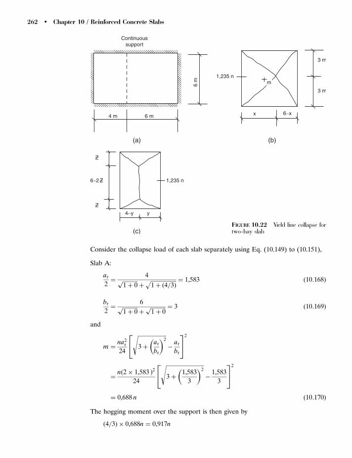
Consider the collapse load of each slab separately using Eq. (10.149) to (10.151),
Slab A:
ar
2¼
4ffiffiffiffiffiffiffiffiffiffiffi1 þ 0
pþ
ffiffiffiffiffiffiffiffiffiffiffiffiffiffiffiffiffiffiffi1 þ ð4=3Þ
p ¼ 1,583 ð10:168Þ
br
2¼
6ffiffiffiffiffiffiffiffiffiffiffi1 þ 0
pþ
ffiffiffiffiffiffiffiffiffiffiffi1 þ 0
p ¼ 3 ð10:169Þ
and
m ¼na2
r
24
ffiffiffiffiffiffiffiffiffiffiffiffiffiffiffiffiffiffiffiffiffi3 þ
ar
br
� �2s
�ar
br
24
35
2
¼nð2 � 1,583 Þ2
24
ffiffiffiffiffiffiffiffiffiffiffiffiffiffiffiffiffiffiffiffiffiffiffiffiffiffiffiffi3 þ
1,583
3
� �2s
�1,583
3
24
35
2
¼ 0,688 n ð10:170Þ
The hogging moment over the support is then given by
ð4=3Þ � 0,688n ¼ 0,917n
4 m 6 m
y4−y
Continuoussupport
6 m m
1,235 n
1,235 n
x 6−x
3 m
3 m
(a) (b)
(c)
Z
6−2 Z
Z
FIGURE 10.22 Yield line collapse fortwo-bay slab
262 � Chapter 10 / Reinforced Concrete Slabs

Slab B:
ar
2¼
6ffiffiffiffiffiffiffiffiffiffiffi1 þ 0
pþ
ffiffiffiffiffiffiffiffiffiffiffiffiffiffiffiffiffiffiffi1 þ ð4=3Þ
p ¼ 2,374 ð10:171Þ
br
2¼
6ffiffiffiffiffiffiffiffiffiffiffi1 þ 0
pþ
ffiffiffiffiffiffiffiffiffiffiffi1 þ 0
p ¼ 3 ð10:172Þ
and
m ¼na2
r
24
ffiffiffiffiffiffiffiffiffiffiffiffiffiffiffiffiffiffiffiffiffi3 þ
ar
br
� �2s
�ar
br
24
35
2
¼nð2 � 2,374 Þ2
24
ffiffiffiffiffiffiffiffiffiffiffiffiffiffiffiffiffiffiffiffiffiffiffiffiffiffiffiffi3 þ
2,374
3
� �2s
�2,374
3
24
35
2
¼ 1,164 n ð10:173Þ
The hogging moment over the support is then given by
ð4=3Þ � 1,164n ¼ 1,552n
There are three alternative approaches to handling the apparent mismatch of
hogging moments:
� Use the value from slab A and re-analyse slab B with a known hogging moment,
� Use the value from slab B and re-analyse slab A with a known hogging moment,
� Use a value lying between those determined and re-analyse both slabs.
In this example, the third approach will be adopted, use a hogging moment of
resistance equal to the mean of the two values determined, i.e. 1,235n.
Slab B:
Consider the yield line pattern in Fig. 10.22(b). This may not be completely correct
but it will give an answer close to the actual value.
Work equation:
n62
3¼
6 � 1,235 nþ 6m
xþ
6m
6 � xþ
2 � 6m
3ð10:174Þ
where the left-hand term is the work done by the load and the right-hand term the
work done by the sagging moment m and the hogging moment 1,235n.
Re-arranging Eq. (10.176) gives
n
m¼
ð6=6x� x2Þ þ ð4=6Þ
2 � ð1,235=xÞð10:175Þ
Concrete Design � 263
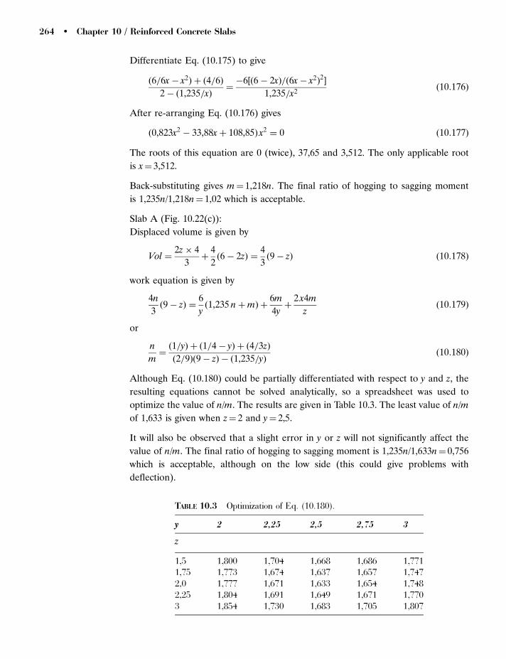
Differentiate Eq. (10.175) to give
ð6=6x� x2Þ þ ð4=6Þ
2 � ð1,235=xÞ¼
�6½ð6 � 2xÞ=ð6x� x2Þ2�
1,235=x2ð10:176Þ
After re-arranging Eq. (10.176) gives
ð0,823x2 � 33,88xþ 108,85Þ x2 ¼ 0 ð10:177Þ
The roots of this equation are 0 (twice), 37,65 and 3,512. The only applicable root
is x¼ 3,512.
Back-substituting gives m¼ 1,218n. The final ratio of hogging to sagging moment
is 1,235n/1,218n¼ 1,02 which is acceptable.
Slab A (Fig. 10.22(c)):
Displaced volume is given by
Vol ¼2z� 4
3þ
4
2ð6 � 2zÞ ¼
4
3ð9 � zÞ ð10:178Þ
work equation is given by
4n
3ð9 � zÞ ¼
6
yð1,235 nþmÞ þ
6m
4yþ
2 x4m
zð10:179Þ
or
n
m¼
ð1=yÞ þ ð1=4 � yÞ þ ð4=3zÞ
ð2=9Þð9 � zÞ � ð1,235=yÞð10:180Þ
Although Eq. (10.180) could be partially differentiated with respect to y and z, the
resulting equations cannot be solved analytically, so a spreadsheet was used to
optimize the value of n/m. The results are given in Table 10.3. The least value of n/m
of 1,633 is given when z¼ 2 and y¼ 2,5.
It will also be observed that a slight error in y or z will not significantly affect the
value of n/m. The final ratio of hogging to sagging moment is 1,235n/1,633n¼ 0,756
which is acceptable, although on the low side (this could give problems with
deflection).
TABLE 10.3 Optimization of Eq. (10.180).
y 2 2,25 2,5 2,75 3
z
1,5 1,800 1,704 1,668 1,686 1,7711,75 1,773 1,674 1,637 1,657 1,7472,0 1,777 1,671 1,633 1,654 1,7482,25 1,804 1,691 1,649 1,671 1,7703 1,854 1,730 1,683 1,705 1,807
264 � Chapter 10 / Reinforced Concrete Slabs

10.7.2 Load Dispersion on to Supporting Beams
An advantage of using the Hillerborg Strip approach is that the loads carried by the
supporting beams may be directly determined from the reactions from the loading
on the individual strips. Yield line analysis, unless combined beam and slab
mechanisms are considered, does not provide the reactions on to supporting
systems. The final yield line pattern does not necessarily provide the load
distribution onto supporting systems, although clearly in some cases it does, e.g.
simply supported square slab.
The need for calculation of beam support loads is often performed assuming the
existence as in the Hillerborg Strip Method of lines indicating load dispersion. It is
common to assume corner lines at 458. This is probably not unreasonable for a slab
with the same edge condition all round the slab, but it may need reassessing where
unequal edge conditions occur.
10.7.3 Shear in One- and Two-way Spanning Slabs
10.7.3.1 Shear Effects from Distributed Loads
The shear at the periphery of a slab is determined from the loading carried to
that support. The shear resistance is determined in the usual manner as for beams,
except that should problems arise with a deficiency in shear capacity, which is rare,
then it is made up by increasing the percentage of reinforcement effective at
the edge being considered. Shear links are never used in normal one or two spanning
slabs.
10.7.3.2 Concentrated Loads
The only loads that need to be considered under this heading are where high
concentrated loads are physically applied to a slab. There is no general need to check
the optional concentrated variable load. Where high concentrated loads are applied
then punching shear needs to be checked around the load. If high concentrated
loads are applied, it may be prudent to consider either a beam and slab assembly or
using the Hillerborg Strip approach to design whereby ‘strong’ strips can be
employed to resist flexure and shear from such loads.
10.8 FLAT SLABSThese will not be covered in any detail, as their flexural design generally follows the
principles above. The problems occur if drop heads are used as failure needs
considering both for the drop head and the slab surrounding the drop head.
Additionally, problems may arise with punching shear. These can be circumvented
Concrete Design � 265
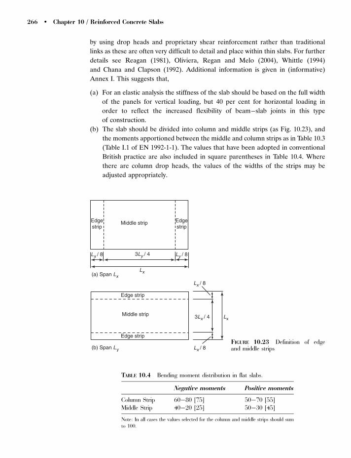
by using drop heads and proprietary shear reinforcement rather than traditional
links as these are often very difficult to detail and place within thin slabs. For further
details see Reagan (1981), Oliviera, Regan and Melo (2004), Whittle (1994)
and Chana and Clapson (1992). Additional information is given in (informative)
Annex I. This suggests that,
(a) For an elastic analysis the stiffness of the slab should be based on the full width
of the panels for vertical loading, but 40 per cent for horizontal loading in
order to reflect the increased flexibility of beam�slab joints in this type
of construction.
(b) The slab should be divided into column and middle strips (as Fig. 10.23), and
the moments apportioned between the middle and column strips as in Table 10.3
(Table I.1 of EN 1992-1-1). The values that have been adopted in conventional
British practice are also included in square parentheses in Table 10.4. Where
there are column drop heads, the values of the widths of the strips may be
adjusted appropriately.
Edgestrip
Edgestrip
Edge strip
Edge strip
Middle strip
(a) Span Lx
(b) Span Ly
Middle strip
Lx
Lx / 8
Lx / 8
Ly / 8
Lx / 8
3Ly / 4
3Lx / 4 Lx
FIGURE 10.23 Definition of edgeand middle strips
TABLE 10.4 Bending moment distribution in flat slabs.
Negative moments Positive moments
Column Strip 60�80 [75] 50�70 [55]Middle Strip 40�20 [25] 50�30 [45]
Note: In all cases the values selected for the column and middle strips should sumto 100.
266 � Chapter 10 / Reinforced Concrete Slabs
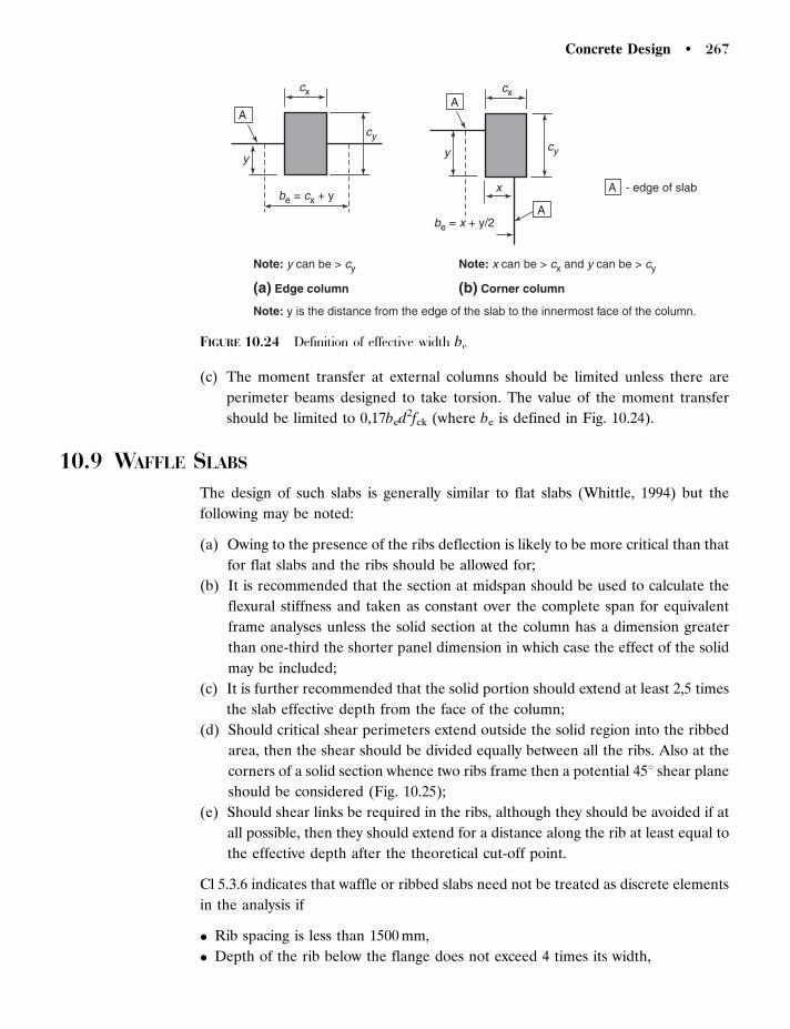
(c) The moment transfer at external columns should be limited unless there are
perimeter beams designed to take torsion. The value of the moment transfer
should be limited to 0,17bed2fck (where be is defined in Fig. 10.24).
10.9 WAFFLE SLABSThe design of such slabs is generally similar to flat slabs (Whittle, 1994) but the
following may be noted:
(a) Owing to the presence of the ribs deflection is likely to be more critical than that
for flat slabs and the ribs should be allowed for;
(b) It is recommended that the section at midspan should be used to calculate the
flexural stiffness and taken as constant over the complete span for equivalent
frame analyses unless the solid section at the column has a dimension greater
than one-third the shorter panel dimension in which case the effect of the solid
may be included;
(c) It is further recommended that the solid portion should extend at least 2,5 times
the slab effective depth from the face of the column;
(d) Should critical shear perimeters extend outside the solid region into the ribbed
area, then the shear should be divided equally between all the ribs. Also at the
corners of a solid section whence two ribs frame then a potential 458 shear plane
should be considered (Fig. 10.25);
(e) Should shear links be required in the ribs, although they should be avoided if at
all possible, then they should extend for a distance along the rib at least equal to
the effective depth after the theoretical cut-off point.
Cl 5.3.6 indicates that waffle or ribbed slabs need not be treated as discrete elements
in the analysis if
� Rib spacing is less than 1500 mm,
� Depth of the rib below the flange does not exceed 4 times its width,
cx cx
AA
A
A - edge of slab
Note: x can be > cx and y can be > cy
Note: y is the distance from the edge of the slab to the innermost face of the column.
Note: y can be > cy
(a) Edge column (b) Corner column
y y
xbe = cx + y
be = x + y/2
cycy
FIGURE 10.24 Definition of effective width be
Concrete Design � 267
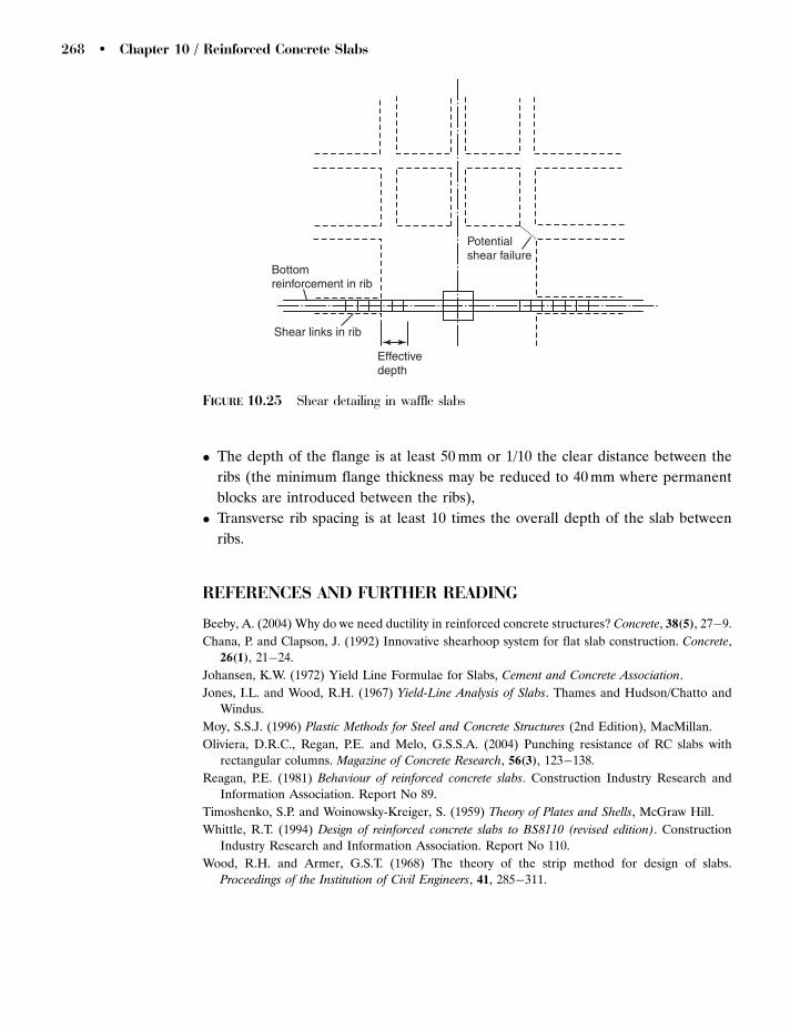
� The depth of the flange is at least 50 mm or 1/10 the clear distance between the
ribs (the minimum flange thickness may be reduced to 40 mm where permanent
blocks are introduced between the ribs),
� Transverse rib spacing is at least 10 times the overall depth of the slab between
ribs.
REFERENCES AND FURTHER READING
Beeby, A. (2004) Why do we need ductility in reinforced concrete structures? Concrete, 38(5), 27�9.
Chana, P. and Clapson, J. (1992) Innovative shearhoop system for flat slab construction. Concrete,
26(1), 21�24.
Johansen, K.W. (1972) Yield Line Formulae for Slabs, Cement and Concrete Association.
Jones, I.L. and Wood, R.H. (1967) Yield-Line Analysis of Slabs. Thames and Hudson/Chatto and
Windus.
Moy, S.S.J. (1996) Plastic Methods for Steel and Concrete Structures (2nd Edition), MacMillan.
Oliviera, D.R.C., Regan, P.E. and Melo, G.S.S.A. (2004) Punching resistance of RC slabs with
rectangular columns. Magazine of Concrete Research, 56(3), 123�138.
Reagan, P.E. (1981) Behaviour of reinforced concrete slabs. Construction Industry Research and
Information Association. Report No 89.
Timoshenko, S.P. and Woinowsky-Kreiger, S. (1959) Theory of Plates and Shells, McGraw Hill.
Whittle, R.T. (1994) Design of reinforced concrete slabs to BS8110 (revised edition). Construction
Industry Research and Information Association. Report No 110.
Wood, R.H. and Armer, G.S.T. (1968) The theory of the strip method for design of slabs.
Proceedings of the Institution of Civil Engineers, 41, 285�311.
Effectivedepth
Shear links in rib
Bottomreinforcement in rib
Potentialshear failure
FIGURE 10.25 Shear detailing in waffle slabs
268 � Chapter 10 / Reinforced Concrete Slabs

C h a p t e r 11 / Foundations andRetaining Walls
This chapter details design considerations for various types of foundations and
retaining walls. Retaining walls are required where it is necessary for part of a
structure to be below ground level, to retain earthworks in a cutting for a road, say,
where due to space full stable slopes are impossible, or may form part of the design
of other parts of structures such as bridge abutments. The function of a foundation is
to transmit the actions from a structure to the underlying ground in such a way that
the bearing strata taking the actions are not over-stressed and that undue defor-
mations occur neither in the structure nor in the ground. The section on foundation
design only considers some of the most common cases. For further information
reference should be made to Henry (1986).
11.1 TYPES OF FOUNDATIONThe type of foundation used in any given case is determined from consideration of
the functions of the foundation, load carrying capacity and minimal deformation,
and the type of load bearing strata available in a given case. Unfortunately, it is often
not possible to determine the details of ground conditions at the start of a design
when the new structure is to be built on the site of existing buildings. This means that
the design of the foundations is often not possible until the latter stages of the design
process. This may cause problems as the structure layout will already have
determined and that a more complex foundation detail will then be needed. It is
absolutely vital that in all cases a full geotechnical survey be carried out not only to
determine the bearing pressures at the level likely to be needed for the foundation
but also below this level where there is a potential likelihood of weak or soft strata
which will cause problems with long term settlement. A properly carried out
geotechnical survey is absolutely essential for any major project, since any long term
problems with the foundations may cause severe structural distress. The cost of
carrying out an appropriate geotechnical survey on any project is only a very small

proportion of the total cost, whereas remedial works to a structure and its environs,
if such a survey is either imperfectly carried out or worse, omitted, may cost many
times the original cost of the new structure.
Typical examples of commonly found structural foundations are illustrated in
Fig. 11.1 and are briefly described as follows.
11.1.1 Simple Unreinforced Strip or Pad Foundation (Fig. 11.1a)
This type of foundation is restricted to the case where the loading is relatively light
with reasonably high bearing pressures. The 458 load dispersion lines must intersect
the sides of the foundation whose width in the case of strip footings is generally
governed by the available widths of excavator buckets. For strip footings carrying
cavity walls it is essential to remember that it is the internal leaf that is the more
heavily loaded and that the centre line of the foundation must coincide with the
resultant load in the two leaves of the wall. It may also be prudent to consider
a nominal eccentricity of 50 to 100 mm for this resultant for consideration of
Loaddispersionlines
Width ≤ spread Width > spread
of dispersion lines
(a) Unreinforced or nominally reinforcedbase
Pile cap
Hard stratum
Friction piles Toe - bearingpiles
Main reinforcement
G.L.
(b) Reinforced base
(c) Combined foundation
(d) Piles
Laps
Kicker
Columnor wall
Columnstarter bars
45° 45°
FIGURE 11.1 Types of foundation
270 � Chapter 11 / Foundations and Retaining Walls
non-uniform bearing pressures due to construction tolerances. Also for long strip
footings nominal mesh reinforcement is often provided.
11.1.2 Pad Foundation (Fig. 11.1(b))
The principal use for a pad foundation is to resist the reaction from a single
concrete column or steel stanchion. Since the reactions are likely to be large then the
area of a pad foundation will be such that the 458 lines will fall within the base. This
means that the area of the base will need to be reinforced in order to carry such
reactions.
11.1.3 Combined Foundations and Raft Foundations (Fig. 11.1(c))
Combined foundations are used where either the column spacing is such that single
pads would overlap or the bearing capacity is low. To avoid differential movement it
is essential that the bearing pressure is uniform over the base. A raft foundation is
simply a combined foundation that extends over the whole of the structure allowing
the structure to behave as an entity. Because of the high loads in the lowest level of
columns in such structures a raft foundation will often be several metres thick in
order to avoid shear failure between the column face and the slab forming the raft.
11.1.4 Piles (Fig. 11.1(d))
These are required where any suitable bearing stratum is at too greater depth for
economic use of any above types owing to the potentially high costs of excavation.
Piles can be divided into two categories: end bearing piles where the load is
transferred to a suitable stratum by bearing on the end of the pile and friction piles
where skin friction between the shaft of the pile and clay strata is mobilized to
transfer the loading. A combination of end bearing and skin friction is also possible.
Piles may also be classified by their method of construction, whether driven or bored.
The possible method of construction must be taken into account when considering
load carrying capacity as bored piles can rarely mobilize skin friction. Pile design is
largely based on experience and empirical methods and will not be considered
further. The reader is referred to Tomlinson (1994) for further information.
11.2 BASIS OF DESIGN
The actual bearing pressure distribution below a foundation is complex as it depends
both upon the stiffness of the foundation (and the structure above) and the physical
properties and deformation characteristics of the strata below the foundation. Whilst
it is possible to determine a distribution using the elastic properties of the ground,
Concrete Design � 271

it is not generally considered necessary. The common simplification is to assume
a linear distribution of bearing pressures (EN 1992-1-1 cl G.1.2). The bearing
pressures or other strength parameters, used in a design should be cautious
estimates based on tests or experience (EN 1997-1 cl 2.4.5.2(3)P). All designs must
have a Geotechnical Design Report as an Annex to the main calculations (EN 1997-
1, cl 2.8). This report must contain details of the assumptions made in the foundation
design together with a summary of the relevant actions and design parameters. It
need not necessarily be a complex report if the foundation design is simple or
straightforward.
EN 1997-1 cl 2.4.7 recognizes five potential limit states:
EQU: This is concerned with equilibrium of the structure or ground
considered as a rigid body where strength of the materials are insignificant
in providing resistance. An example of where this limit state applies is
overturning of a retaining wall, it does not apply to normal foundations.
STR: This is concerned with internal failure or excessive deformation within
the structural materials.
GEO: This is concerned with excessive deformation or failure within the
soil mass.
UPL and HYD: These are concerned with failure due to uplift or hydraulic
heave, respectively.
To size foundations, the limit state STR or GEO is used. UPL and HYD will not be
further considered in this text.
The partial safety factors to be used on actions are given in Table 11.1 (from Table
A.1 and A.3 of EN 1997-1).
For soil parameters the values of the partial safety factors are given in Table 11.2
(from Table A.2 and A.4 of EN 1997-1).
Table 11.3 gives the partial safety factors to be applied to resistances for spread
foundations and earth retaining structures for STR and GEO (from Tables A.5 and
A.13 of EN 1997-1).
EN 1997-1 outlines the possible Design Approaches for STR and GEO that may be
used. These are summarized in Table 11.4.
In all cases partial safety factors are applied to the actions rather than the effects of
the actions. The eventual National Annex to EN 1997-1 may specify the use of one or
more of these Design Approaches (possibly by prohibiting the use of some). As the
National Annex had not been produced at the time of writing the text, the author has
felt it expedient to consider all three, thus making design examples slightly laborious.
272 � Chapter 11 / Foundations and Retaining Walls
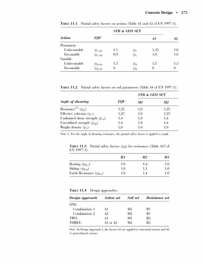
TABLE 11.1 Partial safety factors on actions (Table A1 and A3 of EN 1997-1).
Action EQU
STR & GEO SET
A1 A2
PermanentUnfavourable �G;dst 1,1 �G 1,35 1,0Favourable �G;stb 0,9 �G 1,0 1,0
VariableUnfavourable �Q;dst 1,5 �Q 1,5 1,3Favourable �Q;stb 0 �Q 0 0
TABLE 11.2 Partial safety factors on soil parameters (Table A4 of EN 1997-1).
Angle of shearing EQU
STR & GEO SET
M1 M2
Resistance(1) (��0) 1,25 1,0 1,25Effective cohesion (�c0) 1,25 1,0 1,25Undrained shear strength (�cu) 1,4 1,0 1,4Unconfined strength (�qu) 1,4 1,0 1,4Weight density (��) 1,0 1,0 1,0
Note 1: For the angle of shearing resistance, the partial safety factor is applied to tan�0.
TABLE 11.3 Partial safety factors (�R) for resistances (Table A13 ofEN 1997-1).
R1 R2 R3
Bearing (�R;v) 1,0 1,4 1,0Sliding (�R;h) 1,0 1,1 1,0Earth Resistance (�R;e) 1,0 1,4 1,0
TABLE 11.4 Design approaches.
Design approach Action set Soil set Resistance set
ONECombination 1 A1 M1 R1Combination 2 A2 M2 R1
TWO A1 M1 R2THREE A1 or A2 M2 R3
Note: In Design Approach 3, the factors A1 are applied to structural actions and A2to geotechnical actions.
Concrete Design � 273

11.3 BEARING PRESSURES UNDER FOUNDATIONSUnder no circumstances can tension occur between the ground and the underside of
the base. Further the bearing pressure distribution should be sensibly constant for
the combination of permanent and variable actions (excluding wind or other
accidental actions). Ideally the ratio of maximum to minimum bearing pressures
should not exceed around 1,5 to 2. For cases involving transient load effects such as
wind or other accidental actions this ratio can increase to around 2,5. For retaining
walls a slightly higher value is permissible as some movement must occur in order to
mobilize active or passive pressures (See Section 11.6.1).
Under no account should partial bearing be allowed as this will cause undue rotation
of the base and a possible deleterious redistribution of internal forces in the
structure above the foundation. It is generally accepted that a linear distribution of
bearing pressures may be taken. The moment applied to the base of the foundation
giving rise to the non-linear component of the bearing stress distribution must
include the effect of any horizontal reaction applied at the top face of the
foundation. Thus the total moment MSd,y.net is given by
MSd,y:net ¼ MSd,y þHSd,zh ð11:1Þ
where MSd,y is the moment about the y axis from the structural analysis, HSd,z is the
corresponding horizontal reaction and h is the overall depth of the foundation.
It should be noted that the effect of HSd,z may oppose the effect of MSd,y, in which
case it should probably be neglected.
11.3.1 Uniaxial Moments (Fig. 11.2)
Consider a base of dimensions length L and width B (B�L) with actions NSd and
MSd,y.net. The maximum bearing pressure 1 is given by
1 ¼NSd
AþMSd,y:net
Welð11:2Þ
s2s1
L
NSd
MSd,y,net
FIGURE 11.2 Bearing Pressures due touniaxial bending
274 � Chapter 11 / Foundations and Retaining Walls

where A is the area of the base (BL) and Wel is the elastic section modulus of the
base about the YY axis (BL2/6). The minimum bearing pressure 2 is given by
2 ¼NSd
A�MSd,y:net
Welð11:3Þ
The pressure can be taken as uniform across the width of the base.
11.3.2 Biaxial Bending (Fig. 11.3)
The actions are NSd, MSd, y.net and MSd, z.net and the bearing pressures at each corner
1 to 4 are given by
1 ¼NSd
Aþ
MSd,y:net
Wel,yþ
MSd,z:net
Wel,zð11:4Þ
2 ¼NSd
A�
MSd,y:net
Wel,yþ
MSd,z:net
Wel,zð11:5Þ
3 ¼NSd
A�
MSd,y:net
Wel,y�
MSd,z:net
Wel,zð11:6Þ
4 ¼NSd
Aþ
MSd,y:net
Wel,y�
MSd,z:net
Wel,zð11:7Þ
where Wel, y¼BL2/6 and Wel, z¼LB2/6. Note the maximum bearing stress is 1
and the minimum 3.
MSd,y,net
MSd,z,net
Nsd
y
z
B
s4
s1
s3
s2
L
FIGURE 11.3 Base subjected tobiaxial bending
Concrete Design � 275

The traditional British geotechnical sign convention has been used for bearing
pressures, i.e. compression has been taken as positive. Elsewhere, the stress analysis
sign convention is used, i.e. tension positive (compression negative).
11.3.3 Offset Columns
With high moments at the base of a column and relatively low axial forces the ratio
of the maximum to minimum bearing pressures may be unacceptable. One option
that can be considered is to offset the column from the centre line of the base
(Fig. 11.4).
The net moment applied to the base is then given by
MSd,y:net,1 ¼ MSd,y:net � NSdez1 ð11:8Þ
where ez1 is the displacement between the column and the base centre line.
Note, care must be taken while using this method to equalize bearing stresses, if
it is possible for the moments applied to the foundation to reverse their sense
of application.
EXAMPLE 11.1 Determination of base dimensions. The characteristic actions
applied to a foundation are 300 kN permanent and 350 kN variable together with a
net uniaxial moment. If the ground has a design ultimate bearing pressure of 250 kPa
and the ratio between maximum and minimum bearing pressures is not to exceed
1,5, determine
(a) the width of foundation, if the length is 3 m with characteristic moments of
40 kNm for both the permanent and variable actions, and
(b) suitable base dimensions, if the characteristic moments are 60 kNm permanent
and 80 kNm variable.
In each case, also determine the minimum and maximum design bearing stresses
using the final foundation size.
L /2 L /2
NSd
MSd,y,net
ez1
FIGURE 11.4 Base with offset column
276 � Chapter 11 / Foundations and Retaining Walls

(a) Rearranging Eq. (11.2) gives
B ¼1
1
NSd
Lþ
6MSd,y:net
L2
� �ð11:9Þ
and
B ¼1
2
NSd
L�
6MSd,y:net
L2
� �ð11:10Þ
The only case that needs to be considered is the limit state STR/GEO. In all
cases the load set M1 or M2 does not need considering.
Consider each of the Design Approaches:
Design Approach 1: Combination 1
Action set is A1,
so
NSd ¼ 1,35 � 300 þ 1,5 � 350 ¼ 930 kN
MSd ¼ 1,35 � 40 þ 1,5 � 40 ¼ 114 kNm:
Resistance set is R1, so �R; v¼ 1,0 and des ¼ 250=1,0 ¼ 250 kPa:
From Eq. (11.9)
B ¼ ð930=3 þ 6 � 114=32Þ=250 ¼ 1,544 m
From Eq. (11.10)
B ¼ ð930=3 � 6 � 114=32Þ=ð250=1,5Þ ¼ 1,404 m
Design Approach 1: Combination 2
Action set is A2,
so
NSd ¼ 1,0 � 300 þ 1,3 � 350 ¼ 755 kN
MSd ¼ 1,0 � 40 þ 1,3 � 40 ¼ 92 kNm:
Resistance set is R1, so �R; v¼ 1,0 and des ¼ 250=1,0 ¼ 250 kPa:
From Eq. (11.9)
B ¼ ð755=3 þ 6 � 92=32Þ=250 ¼ 1,252 m
From Eq. (11.10)
B ¼ ð755=3 � 6 � 92=32Þ=ð250=1,5Þ ¼ 1,142 m
Concrete Design � 277

For foundations where there are no actions due to the soil, Combination 1 will
always be critical.
From Combination 1, set B¼ 1,6 m, this will give 1¼ 241 kPa and 2¼ 146 kPa.
Design Approach 2:
Action set is A1,
soNSd ¼ 1,35 � 300 þ 1,5 � 350 ¼ 930 kN
MSd ¼ 1,35 � 40 þ 1,5 � 40 ¼ 114 kNm:
Resistance set is R2, so �R; v¼ 1,4 and des ¼ 250=1,4 ¼ 179 kPa:
From Eq. (11.9)
B ¼ ð930=3 þ 6 � 114=32Þ=179 ¼ 2,156 m
From Eq. (11.10)
B ¼ ð930=3 � 6 � 114=32Þ=ð179=1,5Þ ¼ 1,961 m
This Design Approach would require a base width of 2,2 m giving 1¼ 175 kPa
and 2¼ 106 kPa.
Design Approach 3:
Action set is A1,
soNSd ¼ 1,35 � 300 þ 1,5 � 350 ¼ 930 kN
MSd ¼ 1,35 � 40 þ 1,5 � 40 ¼ 114 kNm:
Resistance set is R3, so �R; v¼ 1,0 and des ¼ 250=1,0 ¼ 250 kPa: This gives the
same results as Design Approach 1: Combination 1.
It would appear that Design Approach 2 gives conservative results for design
of spread foundations.
(b) From Eqs (11.2) and (11.3) the following relationship may be derived
L ¼6MSd,y:net ð1=2Þ þ 1½ �
NSd ð1=2Þ � 1½ �ð11:11Þ
Consider Design Approach 1: Combination 1
Action set is A1,
soNSd ¼ 1,35 � 300 þ 1,5 � 350 ¼ 930 kN
MSd ¼ 1,35 � 60 þ 1,5 � 80 ¼ 201 kNm:
Resistance set is R1, so �R; v¼ 1,0 and des ¼ 250=1,0 ¼ 250 kPa:
278 � Chapter 11 / Foundations and Retaining Walls
From Eq. (11.11)
L ¼ 6 � 201 � ð1,5 þ 1Þ=ð930 � ð1,5 � 1ÞÞ ¼ 6,48 m:
This will give a base width of 0,69 m. This clearly is not an economic solution.
One approach is to offset the column from the base centre line by 100 mm.
From Eq. (11.8), MSd,y,net,1 ¼ 201 � 0,1 � 930 ¼ 108 kNm:
From Eq. (11.11), L¼ 3,48 m with a resultant width of 1,28 m.
Design Approach 1: Combination 2 will give
NSd ¼ 1,0 � 300 þ 1,3 � 350 ¼ 755 kN
MSd ¼ 1,0 � 60 þ 1,3 � 80 ¼ 164 kNm:
Reduced moment with an offset of 100 mm is 164 � 0,1 � 755 ¼ 88,5 kNm.
As these values of MSd and NSd are less than Combination 1, they will not
be critical.
Adopt L¼ 3,5 m and B¼ 1,3 m as practical values. These will give 1¼ 245 kPa
and 2¼ 164 kPa.
Design Approach 2 will not be checked for this particular example.
11.4 CALCULATION OF INTERNAL STRESS RESULTANTS IN PAD FOUNDATIONS
11.4.1 Flexure
11.4.1.1 Longitudinal Bending Moment
Although the critical section is that at the face of the column (EN 1991-1-1,
cl 5.3.2.2(3)), the effective span should be taken to the centre line of the column as
the base should be considered as a continuous cantilever (Fig. 6.13). This will be
slightly conservative when the base is thinner than the column size. Thus, for a
foundation with either no or uniaxially applied moments (Fig. 11.5), the design
moment MSd per unit width of base at the face of the column is
MSd ¼ðL� hc Þ
2
4851 þ 2 þ
hc
L1 � 2ð Þ
� �ð11:12Þ
where hc is the depth of the column.
11.4.1.2 Transverse Bending
The bending moment MSd per unit length is given by
MSd ¼1 þ 2
8B� bcð Þ
2ð11:13Þ
where bc is the width of the column.
Concrete Design � 279

For bases under biaxial bending, analytical expressions may be derived, but it is
sufficiently accurate to use the above expression with 1 taken as the mean of the two
largest adjacent bearing pressures and 2 taken as the mean of the remaining two.
11.4.2 Shear
11.4.2.1 Flexural Shear
This should be checked at a distance equal to the effective depth of the base d
from the face of the column (cl 6.2.1(8)). The value of the applied shear VSd is
given by
VSd ¼d
43 1 þ 2 þ
hc þ 2 d
L1 � 2ð Þ
� �ð11:14Þ
Only VRd, c and VEd, the shear capacities of the concrete alone and due to concrete
crushing, need be checked as it is not usual to supply shear reinforcement. In
addition punching shear may also need checking.
11.4.2.2 Punching Shear
� Column Face
The design shear VSd at the column face should not exceed VEd.
� Successive perimeters
These are at perimeters of 2 d out from the column face and the allowable
shear stress is determined as for normal shear cases except that the reinforcement
ratio, , used is the geometric mean of the reinforcement ratios in the two
orthogonal directions. Care should be taken when part of the critical perimeter
lies outside the area of the base, while only those parts of the perimeter lying
L Flexure
hc
d
d
Shear
s2
s1
FIGURE 11.5 Critical sections for flexuraland shear design
280 � Chapter 11 / Foundations and Retaining Walls

within the base should be considered. Since however the design shear force is
the applied axial force less the effect of the upward reaction on the base, this
case will not usually be critical except for very highly loaded columns on raft
foundations. Where the complete shear perimeter lies within the base, the design
shear force VSd is given by
VSd ¼ NSd �1 þ 2
2Ap ð11:15Þ
where Ap is the area contained within the shear perimeter.
For the purpose of determining shear resistance (and shear reinforcement, if
necessary) foundations are treated as slabs, i.e. if VRd, c is exceeded then 3⁄4VRd, c
may be used in determining the link requirement.
Where the ultimate shear strength VEd is exceeded the base will need thickening
(as the effect of increasing the concrete strength is only marginal and the column
size is generally predetermined).
If the strength VRd, c is exceeded then additional tension reinforcement will need to
be supplied or the base thickened. In general, shear links are not provided in column
bases unless the base is a long thin member supporting a series of column loads in
which case the foundation system will act closer to a beam than a slab. Generally
column bases should not be thinner than around 600 mm.
11.4.3 Anchorage (cl 9.8.2.2)
It is necessary to check the anchorage of tensile reinforcement to resist a force Fs
where Fs is given by
Fs ¼ Rze
zið11:16Þ
where R is the resultant force from the ground pressure, zi is the lever arm between
the centre of compression in the concrete and the tensile reinforcement which may
be taken as 0,9d and ze is the distance between the vertical load NSd and the resultant
R (Fig. 11.6).
The eccentricity e is determined as MSd/NSd subject to a minimum of 015hc. For
notionally straight bars, the critical section may be taken at a distance of x¼ h/2.
11.5 PILE CAPS
These are needed to distribute the loading from the structure or structural element
to the individual piles. Piles are rarely used singly and thus some form of structural
Concrete Design � 281
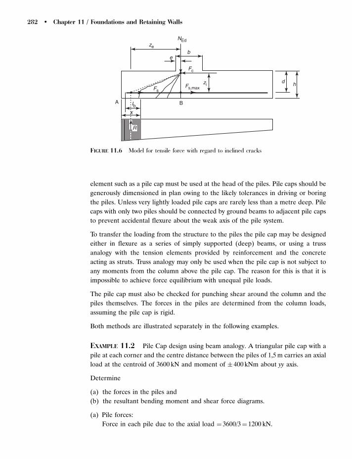
element such as a pile cap must be used at the head of the piles. Pile caps should be
generously dimensioned in plan owing to the likely tolerances in driving or boring
the piles. Unless very lightly loaded pile caps are rarely less than a metre deep. Pile
caps with only two piles should be connected by ground beams to adjacent pile caps
to prevent accidental flexure about the weak axis of the pile system.
To transfer the loading from the structure to the piles the pile cap may be designed
either in flexure as a series of simply supported (deep) beams, or using a truss
analogy with the tension elements provided by reinforcement and the concrete
acting as struts. Truss analogy may only be used when the pile cap is not subject to
any moments from the column above the pile cap. The reason for this is that it is
impossible to achieve force equilibrium with unequal pile loads.
The pile cap must also be checked for punching shear around the column and the
piles themselves. The forces in the piles are determined from the column loads,
assuming the pile cap is rigid.
Both methods are illustrated separately in the following examples.
EXAMPLE 11.2 Pile Cap design using beam analogy. A triangular pile cap with a
pile at each corner and the centre distance between the piles of 1,5 m carries an axial
load at the centroid of 3600 kN and moment of � 400 kNm about yy axis.
Determine
(a) the forces in the piles and
(b) the resultant bending moment and shear force diagrams.
(a) Pile forces:
Force in each pile due to the axial load ¼ 3600/3¼ 1200 kN.
ze
zi
Fc
Fs,maxFs
R
d h
Ibx
B
NEd
be
A
FIGURE 11.6 Model for tensile force with regard to inclined cracks
282 � Chapter 11 / Foundations and Retaining Walls

The force in each pile due to the moment is Mzi/�zi2 where zi is the distance of a
pile from the centroid of the pile cap.
For Pile 1 zi¼ 0,866 m and for Piles 2 and 3, zi¼ 0,433,
soP
z2i ¼ 2 � 0,4332
þ 0,8662¼ 1,125 m2:
Case 1: Moment giving compression in Pile 1
The force in Pile 1 is 400 � ð0,866=1,125Þ ¼ 308 kN (compression), and in piles 2
or 3, 400�(0,433/1,125) ¼ 154 kN (tension).
Total load in Pile 1 is 1200 þ 308 ¼ 1508 kN, and
Total load in Piles 2 or 3 is 1200 � 154 ¼ 1046 kN:
Case 2: Moment giving tension in Pile 1:
Total load in Pile 1 is 1200 � 308 ¼ 892 kN, and
Total load in Piles 2 or 3 is 1200 þ 154 ¼ 1354 kN:
(b) Determination of SFD and BMD
The loading on the pile cap is taken by two beams, the first of which (Beam A)
spans from Pile 1 to the mid-point of Beam B. Beam B spans between Piles 2
and 3.
The loading for both cases on Beam A is given in Fig. 11.7(a) and the resultant
SFD and BMD in Figs 11.7(b) and (c).
The reaction at X is now applied to the centre of Beam B to produce the loading,
SFD and BMD in Fig. 11.8(a) to (c).
Typical reinforcement details for this type of design are given in Fig. 11.9.
EXAMPLE 11.3 Pile Cap design using truss analogy. A triangular pile cap with
a pile at each corner and the centre distance between the piles of s carries an axial
load at the centroid of the pile cap of NSd. Determine the tension force if the
effective depth of the reinforcement is d (Fig. 11.10).
The force in each pile is NSd/3.
For convenience refer to pile 1.
The compression force in the strut between the pile and load point is Cp1, so
resolving vertically
Cp1 sin� ¼NSd
3ð11:17Þ
or
Cp1 ¼NSd
3 sin�ð11:18Þ
Concrete Design � 283

900 776
11641300
(a) Forces on Beam A
(b) SFD's (kN)
(c) BMD's (kNm)
1508
2092
892
2708
3600 kN
400 kNm
1508kN
1
892 kN
400 kNm
3600 kN
0,87 0,43 0,87 0,43
1
FIGURE 11.7 Forces and internal stress resultants on Beam ‘A’
680 880
1046
1046
1354
1354
(2092 kN) (2708 kN)
0,65 0,65 0,650,651046 1354 13541046
2 2 33
(a) Forces on Beam B
(b) SFD's (kN)
(c) BMD's (kNm)
FIGURE 11.8 Forces and internal stress resultants on Beam ‘B’
284 � Chapter 11 / Foundations and Retaining Walls

The tension forces are T12 and T13 and are equal. Resolving horizontally
T12 cos 30 þ T13 cos 30 ¼ Cp1 cos � ð11:19Þ
or
T12 ¼Cp1 cos �ffiffiffi
3p ð11:20Þ
Substitute Eq. (11.18) into Eq. (11.20) to give
T12 ¼NSd
3ffiffiffi3
ptan �
ð11:21Þ
The distance from the centroid to Pile 1 is s/ffiffiffi3
p, thus
tan � ¼d
ffiffiffi3
p
sð11:22Þ
Shearreinforcement
Secondaryreinforcement
Secondaryreinforcement
L
L /2 L /2
L
L
36
33
Mainreinforcement
Mainreinforcement
FIGURE 11.9 Detail of pile cap for three piles
Concrete Design � 285

Substitute Eq. (11.22) into Eq. (11.21) to give
T12 ¼NSd s
9 dð11:23Þ
The area of reinforcement is then determined using a design stress of fyk/�s. This
reinforcement must be anchored in the horizontal plane to ensure there is no
bursting at the top of the pile.
11.6 RETAINING WALLS
Earth Retaining walls are required where either the land take required for a road
cutting is less than that available if natural slope stability were relied on or where it
would be uneconomic to utilize such stability. Retaining walls can be mass concrete
or reinforced concrete (either as plain walls or counterfort walls where the walls are
high) (Fig. 11.11). To a certain extent traditional retaining walls which require a
substantial working area for their execution have been superseded by either
reinforced earth walls, including bridge abutments (Clayton, Milititsky and Woods,
1993) or diaphragm walling which can be executed within the width of a bentonite
slurry filled trench (Henry, 1986). The principles of design for retaining walls also
applies to situations such as water retaining systems for reservoirs.
T13
12
3T13
T12
CP1
s
NSd
NSd
3
NSd
3
NSd
3
f
FIGURE 11.10 Schematic diagram for three pile truss analogy
286 � Chapter 11 / Foundations and Retaining Walls

Only the structural aspects of design are covered and not overall geotechnical
stability such as in Fig. 11.12 which are covered in any standard geotechnics text
book.
11.6.1 Stability of Retaining Walls
Excluding the overall failure mode of Fig. 11.12 a retaining wall needs checking for
(a) Overturning using the limit state of EQU and
(b) Sliding and bearing pressures using the limit states of GEO or STR.
(a) Mass concrete
(b) Cantilever wall
(c) Counterfort retaining wall
Toe
Normally notgreater than2m fill
Height up toaround 7m
Stem
Heel
Counterfort at around2.5–3.5m spacing
Height over 7m
Gravity wall
FIGURE 11.11 Types of retaining wall
Slip planeFIGURE 11.12 Failure by slip insurrounding soil
Concrete Design � 287
Serviceability limits for total and differential settlement or movement may also need
checking. Additionally it is prudent to check cracks widths explicitly for retaining
wall stems.
It is important to note that where surcharge is an unfavourable action, then any
favourable effect should be ignored by not considering the vertical effect within the
zone where the action is favourable (see Examples 11.4 to 11.6).
Where passive pressure is needed to resist actions due to sliding, EN 1997 cl 9.3.2.2 (2)
indicates that the ground level should be lowered to an amount �a, where �a should
be taken as 10 per cent of the distance between the base and the lowest support if
the wall be propped. However, in no case should �a exceed 0,5 m.
To estimate settlement or movement, the following equations (Henry, 1986) may be
used. The settlement s is given by
s ¼2,12B 1 � v2
�Ev
av ð11:24Þ
and the tilt � by
� ¼ arctan5,1 1 � v2
�M0
Ev B2
� �ð11:25Þ
where Ev and v are the Young’s Modulus and Poisson’s ratio of the underlying soil
stratum, B is the width of the base, av the mean bearing pressure at serviceability
limit state beneath the foundation and M0 is moment of the resultant thrust at SLS
about the centre line of the foundation. Annex H of EN 1997-1 gives some guidance
on acceptable levels of displacement and tilt of 50 mm (Annex H cl (4)) and 1/500
(Annex H cl (2)). Clause (2) also suggests the limit on tilt to produce an Ultimate
Limit State is 1/150.
EN 1997 Annex C (cl 8.5.2) an indication of the levels of movement whether lateral
or rotational to develop active or passive earth pressures. The front of a wall
is frequently sloped at around 1 in 25 to mask any slight inevitable tilt. Values of Ev
and v are given in Table 11.5 (Martin, Croxton and Purkiss, 1989). Equations (11.24)
and (11.25) can only provide estimates, and should more exact information be
required, especially where the underlying strata are not able to be categorized by
a single type, then recourse must be made to more complex forms of analysis such
as finite element techniques.
11.6.2 Mass Concrete Retaining Walls
These are generally restricted for economic reasons to heights of around 2 to 3 m
if the section remains of constant thickness (other than any slight front face slope).
288 � Chapter 11 / Foundations and Retaining Walls

It is possible by using stepped walls where the thickness varies with height to exceed
3 m (Henry, 1986). Oliphant (1997) suggests that if the overall height of the wall
including the base is H then the width of the base is between 0,4H and 0,6H with the
wall having a vertical front face and sloping back face. The wall should have an equal
extension of the base from either face with a width at the top of around 300 mm.
EXAMPLE 11.4 Design of a mass concrete retaining wall. The design data for this
example are given in Fig. 11.13.
Overturning is checked using the EQU limit state.
For this case a partial safety factor ��0 is applied to tan�0, thus an effective angle of
friction �eff needs determining from
�eff ¼ arctantan �0
��0
� �ð11:26Þ
With �0 ¼ 308 and ��0 ¼ 1,25, Eq. (11.26) gives a value of �eff¼ 24,88.
The effect of the active earth pressure is given by 0,5Ka�h2, where Ka ¼
ð1 � sin �effÞ=ð1 þ sin�effÞ ¼ 0,409.
TABLE 11.5 Values of Young’s Modulus and Poisson’s ratio for soils(Martin, Croxton and Purkiss, 1989).
Soil type Ev (GPa) v
Dense sand 60�00 0,25Loose sand 15�50 0,30Clayey sands/silts 15�30 0,30Firm and stiff sand clays 2�20 0,35Firm and stiff clays 2�15 0,40Very stiff clays 30�55 0,20
2000
C600
550 550
B
GFED
1500
gc = 25
g = 17 kN/m3
f ′ = δ = 30°
kN /m3
A
100 300K L
J
FIGURE 11.13 Design data for a massconcrete retaining wall
Concrete Design � 289

Moment about point A (Fig. 11.13) due to the earth pressure is
Mearth ¼ 1=3 � 1=2 � Ka � �soil �H3 ¼ 1=3 � 1=2 � 0,409 � 17 � 2,63 ¼ 20,4 kNm=m:
The partial safety factor �G; dst ¼ 1,1, thus factored moment is 1,1 � 20,4 ¼
22,4 kNm=m:
Restoring (or favourable) moment about A is due to the concrete in the base and the
wall and the retained soil mass:
Concrete base:
1=2 � 25 � 0,6 � 1,52¼ 16,9 kNm=m
Concrete wall:
1=2 � 25 � 0,1ð0,55 þ 2=3 � 0,1Þ ¼ 1,5 kNm=m
25 � 2 � 0,3 � ð0,55 þ 0,1 þ 1=2 � 0,3Þ ¼ 12,0 kNm=m
Total due to the concrete¼ 30,4 kNm/m
Retained soil:
17 � 2 � 0,55 � ð1,5 � 1=2 � 0,55Þ ¼ 22,9 kNm=m
Total due to the concrete and earth¼ 53,3 kNm/m
A factor �G; stb of 0,9 must be applied to this, thus the restoring moment is given
by 0,9�53,3¼ 48,0 kNm/m. This is greater than the factored overturning moment
of 22,4 kNm/m, and is therefore satisfactory.
The Limit state of STR/GEO is used to determine sliding and bearing pressures.
Design Approach 1: Combination 1 [A1:M1:R1]
As there is no factor applied to tan�0, �0 ¼ 308 and Ka¼ 1=3.
Moment about centre line of the base due to soil pressure:
1=3 � 1=2 � Ka � �soil �H3 ¼ 1=3 � 1=3 � 1=2 � 17 � 2,63
¼ 16,6 kNm=m ½counterclockwise�
Moment about centre line of the base due to concrete and soil
Base ¼ 0
Wall: 1=2�25�0,1�2�ð0,75�0,55� 1=3�2�0,1Þ¼0,33kNm=m ½counterclockwise�
25�2�0,3�ð0,75�0,55�0,1�1=2�0,15Þ¼�0,75kNm=m ½clockwise�
290 � Chapter 11 / Foundations and Retaining Walls

Net moment due to the concrete is 0,42 kNm/m [clockwise]. The concrete wall can
only have a single partial safety factor attached as it is a single entity, the net effect
must be determined before its state of favourability or unfavourability is determined.
Retained soil:
17 � 2 � 0,55 � ð0,75 � 1=2 � 0,55Þ ¼ 8,88 kNm=m ½clockwise�:
Net moment due to the soil and concrete is 0,42 þ 8,88 ¼ 9,3 kNm=m:
As the higher moment is due to the earth pressure this is the unfavourable moment
and must be factored by �G; dst (¼ 1,35),
so net moment is 1,35 � 16,6 � 9,3 ¼ 13,1 kNm=m
Vertical effects:
Concrete:
Base: 25 � 0,6 � 1,5 ¼ 22,5 kN=m
Wall: 1=2 � 25 � 2 � ð0,3 þ 0,4Þ � 2 ¼ 17,5 kN=m
Total¼ 40,0 kN/m
Soil: 17 � 2 � 0,55 ¼ 18,7 kN=m
Overall Total¼ 58,7 kN/m
Bearing pressures:
For the bearing pressures the vertical action is unfavourable and must be factored by
�G;dst (¼ 1,35), so vertical load is 1,35 � 58,7 ¼ 79,3 kN=m:
1 ¼ 79,3=1,5 þ 6 � 13,1=1,52¼ 88 kPa,
2 ¼ 79,3=1,5 � 6 � 13,1=1,52¼ 18 kPa:
Sliding:
Force due to earth pressure ¼ 1=2KaH2 ¼ 1=2 � 1=3 � 17 � 2,62
¼ 19,2 kN=m:
Apply factor of �G;dst (¼ 1,35) to give 1,35 � 19,2 ¼ 25,9 kN=m
Total (unfactored) vertical load¼ 58,7 kN/m.
Friction force available is 58,7 tan � ¼ 58,7 tan 30 ¼ 33,9 kN=m: This is greater than
the unfavourable action, therefore satisfactory.
Design Approach 1: Combination 2 [A2:M2:R1]
A factor of ��0 is applied to tan�0, so Ka ¼ 0,409 (as in the EQU limit state).
Moment about centre line of the base due to soil pressure:
1=3 � 1=2 � Ka � �soil �H3 ¼ 1=3 � 1=2 � 0,409 � 17 � 2,63¼ 20,4 kNm=m
[counterclockwise]
Concrete Design � 291

Moment about centre line of the base due to concrete and soil:
Base ¼ 0
Wall: 1=2 � 25 � 0,1 � 2 � ð0,75 � 0,55 � 2=3 � 0,1Þ ¼ 0,33 kNm=m [counterclockwise]
25 � 2 � 0,3 � ð0,75 � 0,55 � 0,1 � 1=2 � 0,15Þ ¼ 0,75 kNm=m [clockwise]
Net moment due to the concrete is 0,42 kNm/m [clockwise].
Retained soil:
17 � 2 � 0,55 � ð0,75 � 1=2 � 0,55Þ ¼ 8,88 kNm=m [clockwise].
Net moment due to the soil and concrete is 0,42 þ 8,88 ¼ 9,3 kNm=m [clockwise]
The net moment is 20,4 � 9,3 ¼ 11,1 kNm=m.
Vertical effects:
Concrete:
Base: 25 � 0,6 � 1,5 ¼ 22,5 kN=m
Wall: 1=2 � 25 � 2 � ð0,3 þ 0,4Þ � 2 ¼ 17,5 kN=m
Total¼ 40,0 kN/m
Soil: 17 � 2 � 0,55 ¼ 18,7 kN=m
Overall Total¼ 58,7 kN/m
Bearing pressures:
1 ¼ 58,7=1,5 þ 6 � 11,1=1,52¼ 69 kPa
2 ¼ 58,7=1,5 � 6 � 11,1=1,52¼ 10 kPa:
Sliding:
Force due to earth pressure¼ 1=2KaH2 ¼ 1=2 � 0,409 � 17 � 2,62
¼ 23,5 kN=m:
Total (unfactored) vertical load¼ 58,7 kN/m.
Friction force available is 58,7 tan � ¼ 58,7 tan 30 ¼ 33,9 kN=m: This is greater than
the unfavourable action, therefore satisfactory.
Design Approach 2: [A1:M1:R2]
The action set is the same as Design Approach 1: Combination 1, but the resistance
set [R2] for bearing is 1,4 and sliding 1,1. Thus the maximum permissible bearing
pressure would need to 1,4 times that of Design Approach 1: Combination 1, i.e.
1,4 � 88 ¼ 123 kPa (or if the values in Design Approach 1: Combination were
critical, the base would need to be some 20 to 30 per cent larger).
Sliding: Unfavourable action is 25,9 kN/m (as Design Approach 1: Combination 1).
A factor �R;h (¼ 1,1) is applied to the favourable action, i.e. the available force is
33,89/1,1¼ 30,8 kN/m. This is still satisfactory.
292 � Chapter 11 / Foundations and Retaining Walls
Design Approach 3:
As there are no structural actions, the safety factors applied to the geotechnical
action is Set A2 and the resistance set R3 is equivalent to R1, this approach reduces
to Design Approach 1: Combination 2.
Although the wall has been described as mass concrete it will be prudent to reinforce
the front and back faces of the wall and the lower face of the base with mesh in order
to control cracking and any thermal movement.
11.6.3 Cantilever Retaining Wall
The stability calculations follow those for unreinforced mass retaining walls. The
thickness of the base should be such that no shear reinforcement is necessary. This is
also true of the stem of the wall, together with the requirement that the minimum
thickness of the wall is twice the cover plus the width of two layers (vertical and
horizontal) of reinforcement in both faces and a minimum clearance of 100 mm
between each reinforcement layer to allow full compaction of the concrete. This
generally gives a minimum width of at least 300 mm, although 400 mm may be
preferable. Given the nature of such walls the control of crack widths should be
performed using full calculations using limiting values appropriate to liquid retaining
structures. An allowance needs making for early thermal cracking in addition to
flexural cracking. Oliphant (1997) suggests that for a wall of overall height including
the base, then the base width should lie between 0,5H to 0,8H, the front face of the
wall set back by 0,25B from the front of the base whose thickness should be 0,1H. For
low to moderate heights of wall, the suggested base thickness may be too small as it
could give problems with flexural and shear design. It is therefore recommended that
the minimum base thickness should be around 600 mm.
Shear keys may be necessary to prevent sliding, but a longer heel may help avoid the
problem.
EXAMPLE 11.5 Cantilever retaining wall (Fig. 11.14). For EQU and STR/GEO
where a factor ��0 is applied to tan �0, a shearing angle �eff needs to be determined.
This is given by
�eff ¼ arctantan �0
1,25ð11:27Þ
With �0 ¼ 308, Eq. (11.27) gives �eff¼ 24,88, and
Ka ¼ ð1 � sin�effÞ=ð1 þ sin�effÞ ¼ 0,409:
Concrete Design � 293

EQU:
Overturning moment due to soil:
1=3 � 1=2 � Ka � � �H3 ¼ 1=3 � 1=2 � 0,409 � 17 � 4,33¼ 92,1 kNm=m
Overturning moment due to surcharge:
1=2 � q�H2 ¼ 1=2 � 10 � 4,32¼ 92,5 kNm=m
A factor of �G;dst (¼ 1,1) is applied to the earth pressure and a factor of �Q;dst (¼ 1,5)
is applied to the surcharge, thus the total factored moment is given by
1,1 � 92,1 þ 1,5 � 92,5 ¼ 240,6 kNm=m:
Taking moments about A:
Base: 1=2 � 25 � 0,6 � 3,82¼ 108,3 kNm=m
Wall: 25 � 3,7 � 0,4 � ð0,8 þ 1=2 � 0,4Þ ¼ 37,0 kNm=m
Total ¼ 145,3 kNm/m
Due to the soil:
17 � 3,7 � 2,6 � ð3,8 � 1=2 � 2,6Þ ¼ 408,9 kNm=m
Total ¼ 554,2 kNm/m
A factor �G;stb (¼ 0,9) is applied to the restoring moment, thus the factored restoring
moment is given as 0,9 � 554,2 ¼ 498,8 kNm=m:
This exceeds the factored overturning moment of 240,6 kNm/m, and is therefore
satisfactory.
The Limit state of STR/GEO is used to determine sliding and bearing pressures.
600
A 3800
3700
800
400q = 10 kN/m2
g = 17 kN/m3
gc = 25 kN/m3
f ′ = d = 30°
FIGURE 11.14 Design data for acantilever retaining wall
294 � Chapter 11 / Foundations and Retaining Walls

Design approach 1: Combination 1 [A1: M1: R1]
As there is no factor applied to tan�0, �0 ¼ 308 and Ka¼ 1=3.
Moment about centre line of the base:
due to soil pressure:
1=3 � 1=2 � Ka � �soil �H3 ¼ 1=3 � 1=3 � 1=2 � 17 � 4,33¼ 75,1 kNm=m
[counterclockwise],
due to surcharge:
1=2 � q�H2 ¼ 1=2 � 10 � 4,32¼ 92,5 kNm=m [counterclockwise]
Moment about centre line of the base due to concrete and soil
Base¼ 0
Wall: 1=2 � 25 � 0,4 � 3,7 � ð1=2 � 3,8 � 2=3 � 0,8 � 2=3 � 0,4Þ ¼ 16,7 kNm=m [counter-
clockwise]
Retained soil:
17 � 3,7 � 2,6 � ð1=2 � 3,8 � 1=2 � 2,6Þ ¼ 98,1 kNm=m [clockwise].
A factor of �G of 1,35 is applied to the permanent unfavourable and 1,0 to the
permanent favourable and a factor of �Q of 1,5 to the unfavourable variable.
Taking the counterclockwise direction as unfavourable, the net factored moment is
1,5 � 92,5 þ 1,35 � 75,1 þ 1,35 � 16,7 � 1,0 � 98,1 ¼ 164,6 kNm=m:
Vertical actions:
Concrete:
Base: 25 � 3,8 � 0,6 ¼ 57,0 kN=m
Wall: 25 � 3,7 � 0,4 ¼ 37,0 kN=m
Total due to the concrete¼ 94,0 kN/m
Soil: 17 � 3,7 � 2,6 ¼ 163,5 kN=m
Total vertical action¼ 257,5 kN/m
Sliding:
Factored action due to the surcharge:
�QqH ¼ 1,5 � 10 � 4,3 ¼ 64,5 kN=m
Factored action due to earth pressure:
�G1=2Ka�H
2 ¼ 1,35 � 1=2 � 1=3 � 17 � 4,32¼ 70,7 kN=m
Concrete Design � 295
Total¼ 135,2 kN/m
Available friction force is 257,5tan308¼ 148,7 kN/m. This exceeds the effect of the
surcharge and earth pressure and is therefore satisfactory.
Bearing pressures:
The vertical action being unfavourable needs factoring by �Q, to give
1,35 � 257,5 ¼ 347,6 kN=m:
1 ¼ 347,6=3,8 þ 6 � 164, 6=3, 82¼ 160 kPa,
2 ¼ 347,6=3,8 � 6 � 164, 6=3, 82¼ 23 kPa:
Design Approach 1: Combination 2 [A2:M2:R1]
As there is a factor of 1,25 is applied to tan�0, �eff ¼ 24,88 and Ka¼ 0,409.
Moment about centre line of the base:
due to soil pressure:
1=3 � 1=2 � Ka � �soil �H3 ¼ 1=3 � 1=2 � 0,409 � 17 � 4,33¼ 92,1 kNm=m
[counterclockwise],
due to surcharge:
1=2 � q�H2 ¼ 1=2 � 10 � 4,32¼ 92,5 kNm=m½counterclockwise�
Moment about centre line of the base due to concrete and soil
Base ¼ 0
Wall: 1=2�25�0,4�3,7�ð1=2�3,8�0,8�2=3�0,4Þ¼16,7kNm=m½counterclockwise�
Retained soil:
17 � 3,7 � 2,6 � ð1=2 � 3,8 � 1=2 � 2,6Þ ¼ 98,1 kNm=m [clockwise].
A factor of �G of 1,0 is applied to the permanent unfavourable and favourable
actions and a factor of �Q of 1,3 to the unfavourable variable.
Taking the counterclockwise direction as unfavourable, the net factored moment is
1,3 � 92,5 þ 1,0 � 92,1 þ 1,0 � 16,7 � 1,0 � 98,1 ¼ 131 kNm=m:
Vertical actions:
Concrete:
Base: 25 � 3,8 � 0,6 ¼ 57,0 kN=m
Wall: 25 � 3,7 � 0,4 ¼ 37,0 kN=m
Total due to the concrete¼ 94,0 kN/m
296 � Chapter 11 / Foundations and Retaining Walls

Soil: 17 � 3,7 � 2,6 ¼ 163,5 kN=m
Total vertical action¼ 257,5 kN/m
Sliding:
Factored action due to the surcharge:
�QqH ¼ 1,3 � 10 � 4,3 ¼ 55,9 kN=m
Factored action due to earth pressure:
�G1=2Ka�H
2 ¼ 1,0 � 1=2 � 0,409 � 17 � 4,32¼ 64,3 kN=m
Total ¼ 123,2 kN/m
Available friction force is 257,5tan308¼ 148,7 kN/m. This exceeds the effect of the
surcharge and earth pressure and is therefore satisfactory.
Bearing pressures:
The vertical action being unfavourable needs factoring by �Q, to give
1,0 � 257,5 ¼ 257,5 kN=m:
1 ¼ 257, 5=3, 8 þ 6 � 131=3, 82¼ 122 kPa,
2 ¼ 257, 5=3, 8 � 6 � 131=3, 82 ¼ 13 kPa:
Design Approach 2:
This essentially follows Design Approach 1: Combination 1, except that
(a) The available friction force of 148,7 kN/m needs to be factored by �R;h (¼ 1,1) to
give 148,7/1,1¼ 135,2 kN/m. This equals the unfavourable force due to earth
pressure and surcharge of 135,2 kN/m.
(b) The maximum allowable bearing pressure would need to be 1,4 (�R;v) higher.
Design Approach 3:
In this case the factors applied to geotechnical actions are Set A1 and to structural
actions A2. It is assumed the surcharge is a structural action. The soil set is M2 and
the Resistance set is R3 (equivalent to R1).
As there is a factor of 1,25 is applied to tan�0, �eff ¼ 24,88 and Ka¼ 0,409.
Moment about centre line of the base:
due to soil pressure:
1=3 � 1=2 � Ka � �soil �H3 ¼ 1=3 � 1=2 � 0,409 � 17 � 4,33¼ 92,1 kNm=m
[counterclockwise],
due to surcharge:
1=2 � q�H2 ¼ 1=2 � 10 � 4,32¼ 92,5 kNm=m [counterclockwise]
Concrete Design � 297
Moment about centre line of the base due to concrete and soil
Base¼ 0
Wall : 1=2 � 25 � 0,4 � 3,7 � ð1=2 � 3,8 � 0,8 � 2=3 � 0,4Þ ¼ 16,7 kNm=m
[counterclockwise]
Retained soil:
17 � 3,7 � 2,6 � ð1=2 � 3,8 � 1=2 � 2,6Þ ¼ 98,1 kNm=m ½clockwise�:
A factor of �G of 1,0 is applied to the permanent favourable actions and a factor of
�G of 1,0 to the permanent unfavourable (geotechnical) and a �G of 1,5 to the
unfavourable variable.
Taking the counterclockwise direction as unfavourable, the net factored moment is
1,5 � 92,5 þ 1,0 � 92,1 þ 1,0 � 16,7 � 1,0 � 98,1 ¼ 149,5 kNm=m:
Vertical actions:
Concrete:
Base: 25 � 3,8 � 0,6 ¼ 57,0 kN=m
Wall: 25 � 3,7 � 0,4 ¼ 37,0 kN=m
Total due to the concrete¼ 94,0 kN/m
Soil: 17 � 3,7 � 2,6 ¼ 163,5 kN=m
Total vertical action¼ 257,5 kN/m
Sliding:
Factored action due to the surcharge:
�QqH ¼ 1,5 � 10 � 4,3 ¼ 64,5 kN=m
Factored action due to earth pressure:
�G1=2Ka�H
2 ¼ 1,0 � 1=2 � 0,409 � 17 � 4,32¼ 64,3 kN=m
Total¼ 28,8 kN/m
Available friction force is 257,5 tan 308¼ 148,7 kN/m. This exceeds the effect of the
surcharge and earth pressure and is therefore satisfactory.
Bearing pressures:
The vertical action being unfavourable needs factoring by �Q [Set A1], to give
1,35 � 257,5 ¼ 347,6 kN=m:
1 ¼ 347,6=3,8 þ 6 � 149, 5=3, 82¼ 154 kPa,
2 ¼ 347,6=3,8 � 6 � 149, 5=3, 82¼ 29 kPa:
298 � Chapter 11 / Foundations and Retaining Walls

To summarize the results of the various design approaches it will be noted that
Design Approach 2 is the most conservative as the sliding calculations only just work
and would require a larger base (or higher permissable bearing pressures). There
would appear to be little to choose between the other design approaches except that
Design Approach 1 requires two combinations to be considered.
It is intended to use Design Approach 1 to determine the stress resultants to carry
out the structural design. Only combination 1 will be considered as this produces
higher forces.
This is used for the structural design.
With �¼ 308, Ka¼ 0,333
For exposure Class XC2 (Foundations) with a concrete strength of C40/50, structure
Class is SC3 (as the concrete strength reduces the basic class SC4 by 1), cmin,dur is
20 mm. The final design cover cnom is given by cmin þ�cdev ¼ 20 þ 10 ¼ 30 mm:
Design of stem:
Effective depth (assuming 25 mm bars):
d ¼ 400 � 30 � 25=2 ¼ 357,5 mm: Use d¼ 355 mm.
Flexural design:
At the base of the stem take the effective span as the length of the cantilever plus
half the base thickness, i.e.
3,7 þ 1=2 � 0,6 ¼ 4 m,
MSd ¼ 1,35 � 1=2 � 1=3 � 1=3 � 17 � 43Þ þ 1,5 � 1=2 � 10 � 42
¼ 201,6 kNm=m
MSd=bd2fck ¼ 201,6 � 103=ð40 � 3552
Þ ¼ 0,04
From Eq. (6.22),
As fyk
bd fck¼ 0,652 �
ffiffiffiffiffiffiffiffiffiffiffiffiffiffiffiffiffiffiffiffiffiffiffiffiffiffiffiffiffiffiffiffiffiffiffiffiffiffiffi0,425 � 1,5
MSd
b d2 fck
s
¼ 0,652 �ffiffiffiffiffiffiffiffiffiffiffiffiffiffiffiffiffiffiffiffiffiffiffiffiffiffiffiffiffiffiffiffiffiffiffiffiffi0,425 � 1,5 � 0,04
p¼ 0,048 ð11:28Þ
As ¼ 0,048 � 1000 � 355 � 40=500 ¼ 1363 mm2=m: Fix D20 at 200 mm spacing
[1572 mm2/m].
The maximum shear may be determined at d above the top of the base, i.e. at
4 � 0,355 ¼ 3,645 m:
VSd ¼ 1,35 � 1=2 � 1=3 � 17 � 3,6452 þ 1,5 � 10 � 3,645 ¼ 105,5 kN=m:
Concrete Design � 299

Shear:
VEd ¼ 0,5vfcdbwd
v ¼ 0,6ð1 � fck=250Þ ¼ 0,6ð1 � 40=250Þ ¼ 0,504
fcd ¼ fck=�c ¼ 40=1,5 ¼ 26,7 MPa:
VEd ¼ 0,5 � 0,504 � 26,7 � 1000 � 355Þ � 10�3¼ 2388 kN=m4VSd
With no axial force (ignoring self weight of the stem):
VRdc ¼ CRd,ckð1001fckÞ1=3bd
1 ¼ As=bd ¼ 1572=ð1000 � 355Þ ¼ 0,0044350,02
CRd,c ¼ 0,18=�c ¼ 0,18=1,5 ¼ 0,12
k ¼ 1 þffiffiffiffiffiffiffiffiffiffiffiffiffi200=d
p¼ 1 þ
ffiffiffiffiffiffiffiffiffiffiffiffiffiffiffiffiffi200=355
p¼ 1,7552,0
VRdc ¼ 0,12� 1,75� ð100� 0,00443� 40Þ1=3 � 355� 1000� 10�3¼194,4 kN=m4VSd,
Therefore no shear reinforcement required.
As there is the possibility of water, crack widths need explicit calculation Table 7.1N
of EN 1992-1-2 indicates that for exposure class XC2 the limiting crack width is
0,3 mm. Consider the surcharge always at its full value.
MSd ¼ 1=3 � 1=3 � 1=2 � 17 � 43þ 1=2 � 10 � 42 ¼ 140,4 kNm=m
Determine critical spacing from (Section 5.2.2.1):
5(c þ �/2) ¼ 5(30 þ 20/2) ¼ 200 mm. Actual spacing is 200 mm, therefore treat as
close spaced (cl 7.3.4 (3)).
sr,max ¼ 3,4cþ 0,425k1k2�=p,eff
k1 ¼ 0,8 ðhigh bond barsÞ
k2 ¼ 0,5 ðflexureÞ
Determine neutral axis depth x:
Ecm ¼ 22ðð fck þ 8Þ=10Þ0,3¼ 22ð40 þ 8Þ=10Þ0,3
¼ 32 GPa:
Es ¼ 200 GPa; �e ¼ Es=Ecm ¼ 200=32 ¼ 6,25
�e ¼ 0,00443 � 6,25 ¼ 0,0277:
From Eq. (5.25),
x
d¼ �e
ffiffiffiffiffiffiffiffiffiffiffiffiffiffiffiffiffi1 þ
2
�e
s� 1
" #
¼ 0,0277
ffiffiffiffiffiffiffiffiffiffiffiffiffiffiffiffiffiffiffiffiffiffi1 þ
2
0,0277
s� 1
" #¼ 0,209 ð11:29Þ
x¼ 0,209� 355¼ 74,2 mm.
300 � Chapter 11 / Foundations and Retaining Walls

Determine hc,ef:
2,5ðh� dÞ ¼ 2,5ð400 � 355Þ ¼ 112,5 mm; ðh� xÞ=3 ¼ ð400 � 74,2Þ=3 ¼ 108,6 mm;
h=2 ¼ 400=2 ¼ 200 mm
The least of these values is 108,6 mm.
Ac,eff ¼ 1000 � 108,6 ¼ 108600 mm2:
p,eff ¼ As=Ac,eff ¼ 1572=108600 ¼ 0,0145
sr,max ¼ 3,4 � 30 þ 0,425 � 0,8 � 0,5 � 20=0,0145 ¼ 366 mm:
Determine the crack width wk from Eq. (5.31)
wk ¼ sr,maxð"sm � "cmÞ
where "sm� "sm is given by Eq. (5.32),
"sm � "cm ¼s � ktð fct,eff=p,effÞ 1 þ �ep,eff
�Es
� 0,6s
Esð11:30Þ
Determine Icr from Eq. (5.24),
Icr
bd3¼
1
3
x
d
� �3þ�e 1 �
x
d
� �2
¼1
3� 0, 2093
þ0,0277ð1 � 0,209 Þ2 ¼ 0,204 ð11:31Þ
Icr ¼ 0,0204 � 1000 � 3553¼ 0,913 � 109 mm4
s ¼ �eMðd� xÞ=Icr ¼ 6,25 � 140,4 � 106� 355ð1 � 0,209Þ=0,913 � 109
¼ 270 MPa
Determine fct,eff:
This may be taken as fctm ¼ 0,3ð fckÞ2=3
¼ 0,3ð40Þ2=3 ¼ 3,5 MPa
The loading may be considered long term, thus kt¼ 0,4.
Thus "sm� "sm is
"sm � "cm ¼270 � 0,4ð3,5=0,0145Þ 1 þ 6,25 � 0,0145ð Þ
200 � 103
¼ 823,5 � 10�6 ð11:32Þ
Check limiting value of "sm� "sm:
0,6s=Es ¼ 0,6 � 270=200 � 103¼ 810 � 10�6:
Thus "sm� "sm is 823,5�10-6, and
wk ¼ sr,maxð"sm � "smÞ ¼ 366 � 823,5 � 10�6¼ 0,30 mm:
Concrete Design � 301

Wall deflection using span-effective depth ratio:
Steel ratio ¼ 1572=355 � 1000 ¼ 0,00443
0 ¼ 0,001ffiffiffiffiffifck
p¼ 0,001 �
ffiffiffiffiffi40
p¼ 0,00632
For a cantilever K¼ 0,4, as 5 0, so l/d is given by
l
d¼ K 11 þ 1,5
ffiffiffiffiffifck
p 0
þ 3,2
ffiffiffiffiffifck
p 0
� 1
� �3=2" #
¼ 0,4 11 þ 1,5ffiffiffiffiffi40
p 0,00636
0,00443þ 3,2
ffiffiffiffiffi40
p 0,00636
0,00443� 1
� �3=2" #
¼ 12,2 ð11:33Þ
Actual span/effective depth¼ 4000/355¼ 11,3. This is less than the allowable,
therefore satisfactory.
Longitudinal Reinforcement:
This is needed to prevent early thermal cracking. Use Anchor (1992), as a data
source for temperature rise. Anchor indicates that the crack width wk due to early
cracking may be calculated as
wk ¼ 0,5� �1 þ �2ð Þ sr,max ð11:34Þ
where sr,max is the maximum spacing of the cracks, � is the coefficient of thermal
expansion of the concrete (10�strain/8C (cl 3.1.2.5.4)), �1 is the temperature
generated due the dissipation of the heat of hydration of the cement and �2 is
temperature dependant upon the time of year in which the concreting took place.
The 0,5 factor appears in Eq. (11.34) as an indication that there is in normal practice
some restraint to free thermal expansion.
Determination of �1 and �2:
From Anchor (1992), �2 should be taken in the UK as 108C for winter concreting and
208C for summer. Take �2 as 208C (conservative).
From Table 5.3 (Anchor, 1992) �1 for a wall thickness of 400 mm, cement content of
350 kg/m3 and 18 mm plywood formwork may be taken as 378C (interpolating).
Use a design crack width of 0,3 mm to determine sr,max.
sr,max ¼ wk=0,5�ð�1 þ �2Þ ¼ 0,3=ð0,5 � 10 � 10�6� ð37 þ 20ÞÞ ¼ 1053 mm
Determination of steel:
Anchor gives the following equation for sr,max:
sr,max ¼fctm
fb
�
2cð11:35Þ
302 � Chapter 11 / Foundations and Retaining Walls

where � is the bar diameter, fctm is the tensile strength of the concrete, fbd is the bond
strength and c is the reinforcement area. Note that in Eq. (11.35) the partial safety
factor has been omitted from both fbd and fctm as only the ratio between the two
values is required.
From cl 8.4.5.2(2), fbd is given by fbd ¼ 2,25�1�2 fctd ¼ 2,25�1�2 fctm=�c:
Thus fctm=fb ¼ 1=ð2,25�1�2Þ
�1: Conservatively 0,7
�2: 1,0 (bar size less than 32)
fctm=fb ¼ 1 = ð2,25�1�2Þ ¼ 1 = ð2,25 � 0,7 � 1,0Þ ¼ 40=63: It should be noted that
this value closely agrees with the value of 2=3 for type 2 bars quoted in Table 5.2
of Anchor (1992).
Equation (11.35) becomes
sr,max ¼40
63
�
2 cð11:36Þ
For a thickness less than 500 mm, As should be calculated on the basis of an effective
concrete thickness of h/2 and for thicknesses greater than 500, an effective concrete
thickness of 250 mm (Anchor, 1992). In this case the wall is 400 thick at the top and
800 at the bottom. As the majority of the wall is thicker than 500 use 250 mm
effective thickness.
If the spacing of the reinforcement is s,
then As ¼ ð1000 = sÞ �2 = 4,
c ¼ As = ð250 � 1000Þ ¼ 4 � 10�6 As, therefore
c ¼ 4 � 10�6ð1000=sÞ �2=4 ¼ 0,00314�2=s: Thus �=c ¼ 318s=�:
From Eq. (11.36),
sr,max ¼40
63
�
2 c¼
40
63�
1
2� 318
s
�¼ 101
s
�ð11:37Þ
smax¼ 1052 mm (from above), so ðs=�Þreq ¼ 1052=101 ¼ 10,4 mm
Use D10 at 100 ctrs (As¼ 785 mm2/m) each face.
Base:
1 ¼ 154 kPa (at A) and 2 ¼ 29 kPa (at B)
Design of reinforcement:
Based on an estimate of 32 mm bars, d ¼ 600 � 30 � 16 ¼ 554 mm:
Concrete Design � 303

Use d¼ 550 mm.
Moment at front of wall due to bearing pressure (Fig. 11.15):
MSd ¼ 128 � 0,8ð1=2 � 0,8 þ 0,2Þ þ 1=2ð154 � 128Þ � 0,8ð2=3 � 0,8 þ 0,2Þ ¼ 69 kNm=m
Moment at rear of wall due to bearing pressure:
MSd ¼ 29� 2,6ð1=2� 2,6þ 0,2Þþ 1=2 ð115� 29Þ� 2,6ð1=3� 2,6þ 0,2Þ ¼ 232kNm=m
MSd=bd2fck ¼ 232� 103=ð5502
� 40Þ ¼ 0,0192:
From Eq. (6.22) As fyk=bdfck ¼ 0,0226;As ¼ 994 mm2=m:
Fix D16 at 200 mm spacing (to line up with vertical steel) [1005 mm2/m].
Shear at ‘d’ from either face of the wall.
Front face:
Vsd ¼ 1=2 � 0,25ð154 þ 148Þ ¼ 37,8 kN=m
Back face:
Vsd ¼ 1=2 � 2,05ð98 þ 29Þ ¼ 130,2 kN=m
Check shear capacity VRdc only.
VRdc ¼ CRd,ckð1001 fckÞ1=3bd
1 ¼ As=bd ¼ 1005=ð1000 � 550Þ ¼ 0,0018350,02
CRd,c ¼ 0,18=�c ¼ 0,18=1,5 ¼ 0,12
k ¼ 1 þffiffiffiffiffiffiffiffiffiffiffiffiffi200=d
p¼ 1 þ
ffiffiffiffiffiffiffiffiffiffiffiffiffiffiffiffiffi200=550
p¼ 1,6352,0
0,80,55
0,4
2,6
0,55
154 kPa29 kPa
148 128 115 98
FIGURE 11.15 Ultimate bearingpressure distribution
304 � Chapter 11 / Foundations and Retaining Walls

VRdc ¼ 0,12 � 1,63 � ð100 � 0,00183 � 40Þ1=3 � 550 � 1000 � 10�3 ¼ 209 kN=m4VSd,
Therefore no shear reinforcement required.
Anchorage (cl 9.8.2.2)
Front face:
Take x¼ h/2¼ 250 mm.
R ¼ 1=2ð154 þ 148Þ � 0,25 ¼ 37:8 kN=m
e ¼ 0,15b ¼ 0,15 � 400 ¼ 60 mm
ze ¼ 800 � x=2 þ e ¼ 800 � 1=2 � 250 þ 60 ¼ 735 mm
zi ¼ 0,9d ¼ 0,9 � 550 ¼ 495 mm
Fs ¼ Rze=zi ¼ 37,8 � 735=495 ¼ 56,1 kN=m:
There are five bars per metre, therefore force per bar¼ 56,1/5¼ 11,2 kN.
Bond strength ¼ 2,25 � 0,7 � 1,0 � 3,5=1,5 ¼ 3,68 MPa:
Perimeter of bar¼ 16 ¼ 50 mm.
Anchorage length ¼ 11200/(50�3,67)¼ 61 mm. This is less than x, therefore there
are no anchorage problems.
Back face:
Take x¼ h/2¼ 250 mm.
R ¼ 1=2ð29 þ 37Þ � 0,25 ¼ 8,25 kN=m
e ¼ 0,15b ¼ 0,15 � 400 ¼ 60 mm
ze ¼ 800 � x=2 þ e ¼ 2600 � 1=2 � 250 þ 60 ¼ 2535 mm
zi ¼ 0,9d ¼ 0,9 � 550 ¼ 495 mm
Fs ¼ R ze=zi ¼ 8,25 � 2535=495 ¼ 42,3 kN=m:
This is less than the figure for the front face.
Longitudinal steel:
From cl 9.3.1.1(2), the distribution reinforcement should be at least 20 per cent of
the main longitudinal reinforcement.
As ¼ 1005 mm2m; 0,2As ¼ 201 mm2=m: Minimum steel ¼ 0,0013bd ¼ 0,0013 � 550
�1000 ¼ 715 mm2: Maximum spacing 450 mm or 3,5h (¼ 1,75 m). Fix D12 at 150
centres (A¼ 754 mm2/m).
Settlement and tilt:
Assuming dense sand Ev¼ 80 MPa and v¼ 0,3.
Serviceability analysis:
Ka¼ 1=3.
Concrete Design � 305

Moment about centre line of the base:
due to soil pressure:
1=3� 1=2�Ka��soil�H3 ¼ 1=3� 1=3� 1=2�17�4,33¼75,1kNm=m ½counterclockwise�,
due to surcharge:
1=2 � q�H2 ¼ 1=2 � 10 � 4,32¼ 92,5 kNm=m ½counterclockwise�
Moment about centre line of the base due to concrete and soil
Base¼ 0
Wall: 1=2�25�0,4�3,7�ð1=2�3,8�0,8�2=3�0,4Þ¼16,7kNm=m [counterclockwise]
Retained soil:
17 � 3,7 � 2,6 � ð1=2 � 3,8 � 1=2 � 2,6Þ ¼ 98,1 kNm=m [clockwise].
Taking the counterclockwise direction as unfavourable, the net moment is
92,5 þ 75,1 þ 16,7 � 98,1 ¼ 86,2 kNm=m:
Vertical actions:
Concrete:
Base: 25 � 3,8 � 0,6 ¼ 57,0 kN=m
Wall: 25 � 3,7 � 0,4 ¼ 37,0 kN=m
Total due to the concrete:¼ 94,0 kN/m
Soil: 17 � 3,7 � 2,6 ¼ 163,5 kN=m
Total vertical action¼ 257,5 kN/m
Bearing pressures:
1 ¼ 257,5=3,8 þ 6 � 86,2=3,82¼ 104 kPa,
2 ¼ 257,5=3,8 � 6 � 86,2=3,82¼ 32 kPa:
The average bearing pressure is needed at serviceability together with the service out
of balance moment. Assuming dense sand Ev¼ 80 GPa (from Table 11.5).
The average bearing pressure av ¼ 0,5ð104 þ 32Þ ¼ 68 kPa:
B¼ 3,8 m, so from Eq. (11.24),
s ¼ 2,12 � 3,8 � ð1 � 0,32Þ � 68=80 ¼ 6,2 mm
Out of balance moment M0¼ 86,2 kNm/m, so from Eq. (11.25) the angle of tilt �
is given as
� ¼ arctan ð5,1 � ð1 � 0,32Þ � 86,2 � 103=ð80 � 38002
ÞÞ ¼ 0,0198:
306 � Chapter 11 / Foundations and Retaining Walls

Movement at top of wall¼ 400� tan0,0198¼ 1,4 mm (mov/h¼ 1/280)
EN 1997-1 Table C.1 suggests that a rotational movement of the order 0,004 to
0,005H is required for dense sand to mobilize active pressures. In this case the
rotational movement is around 0,0036H not including the effect of deflection of the
wall. Thus active pressures should be capable of being mobilized.
11.6.4 Counterfort Retaining Walls
These are needed when the height exceeds around 7 m, although an alternative
option is to use normal plain stem retaining walls with the addition of ground
anchors to resist part of the effects of the lateral thrust. Typical dimensions of a
counterfort retaining wall are given in Fig. 11.16. Full joints are usual at around 20 to
30 m. To carry out the initial stability and bearing pressure calculations the specific
Section A-A
Elevation Joint
S
S / 20
0.7S 0.7S A
A
S
Plan250 minimum
1m 25 batter Counterfort
FIGURE 11.16 General arrangement of a counterfort retaining wall
Concrete Design � 307
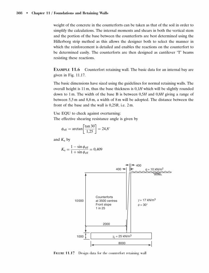
weight of the concrete in the counterforts can be taken as that of the soil in order to
simplify the calculations. The internal moments and shears in both the vertical stem
and the portion of the base between the counterforts are best determined using the
Hillerborg strip method as this allows the designer both to select the manner in
which the reinforcement is detailed and enables the reactions on the counterfort to
be determined easily. The counterforts are then designed as cantilever ‘T’ beams
resisting these reactions.
EXAMPLE 11.6 Counterfort retaining wall. The basic data for an internal bay are
given in Fig. 11.17.
The basic dimensions have sized using the guidelines for normal retaining walls. The
overall height is 11 m, thus the base thickness is 0,1H which will be slightly rounded
down to 1 m. The width of the base B is between 0,5H and 0,8H giving a range of
between 5,5 m and 8,8 m, a width of 8 m will be adopted. The distance between the
front of the base and the wall is 0,25B, i.e. 2 m.
Use EQU to check against overturning:
The effective shearing resistance angle is given by
�eff ¼ arctantan 30
1,25
� �¼ 24,8
and Ka by
Ka ¼1 � sin�eff
1 þ sin�eff¼ 0,409
400
10000
1000
2000
8000
gc = 25 kN/m3
g = 17 kN/m3
f = 30°
400q = 10 kN/m2
Counterfortsat 3500 centresFront slope1 in 25
FIGURE 11.17 Design data for the counterfort retaining wall
308 � Chapter 11 / Foundations and Retaining Walls

Moment about A due to earth pressure:
1=3 � 1=2 � Ka � � �H3 ¼ 1=3 � 1=2 � 0,409 � 17 � 113¼ 1542 kNm=m
due to surcharge:
1=2 � q�H2 ¼ 1=2 � 10 � 112¼ 605 kNm=m
Apply a factor �G;dst (¼ 1,1) to the earth pressure and �Q;dst (¼ 1,5) to the surcharge
to give a factored overturning moment of
1,1 � 1542 þ 1,5 � 605 ¼ 2604 kNm=m:
Restoring moment:
Concrete:
Base: 1=2 � 25 � 1,0 � 8,02 ¼ 800 kNm=m
Wall: 1=2 � 25 � 10 � 0,4 � ð2 þ 2=3 � 0,4Þ ¼ 113 kNm=m
25 � 10 � 0,4 � ð2 þ 0,4 þ 1=2 � 0,4Þ ¼ 260 kNm=m
Total¼ 1173 kNm/m
Retained earth:
17 � 10 � 5,2ð8 � 1=2 � 5,2Þ ¼ 4774 kNm=m
Total unfactored restoring moment¼ 5947 kNm/m
This takes a factor �G;dst (¼ 0,9) to give a net restoring moment of
0,9�5947¼ 5352 kNm/m. This is greater than the overturning moment and is
therefore satisfactory.
STR/GEO:
For this example only Load Case 1 Combination 1 will be considered. For this case
tan�0 is unfactored and Ka¼ 1=3.
Taking moments about the base centre line.
Earth pressure:
1=3 � 1=2 � Ka � � �H3 ¼ 1=3 � 1=3 � 1=2 � 17 � 113¼ 1257 kNm=m
due to surcharge:
1=2 � q�H2 ¼ 1=2 � 10 � 112¼ 605 kNm=m
Restoring moment:
Concrete:
Base: ¼ 0
Wall: 1=2 � 25 � 10 � 0,4 � ð4 � ð2 þ 2=3 � 0,4ÞÞ ¼ 87 kNm=m
25 � 10 � 0,4 � ð4 � ð2 þ 0,4 þ 1=2 � 0,4ÞÞ ¼ 227 kNm=m
Total¼ 227 kNm/m [counterclockwise]
Concrete Design � 309
Retained earth:
17 � 10 � 5,2 � ð4 � 1=2 � 5,2Þ ¼ 1238 kNm=m [clockwise]
Apply a factor of �G of 1,0 to the favourable permanent loads, a factor � of 1,35 to
the permanent unfavourable and �Q of 1,5 to unfavourable variable to give a net
factored unfavourable moment of 1,5 � 605 þ 1,35 � 1257 þ 1,35 � 227 � 1,0�
1238 ¼ 1673 kNm=m:
Vertical:
Concrete:
Base: 25 � 8 � 1 ¼ 200 kN=m
Wall: 1=2 � 25 � ð0,4 þ 0,8Þ � 10 ¼ 150 kNm=m
Total¼ 350 kN/m
Soil: 17 � 10 � 5,2 ¼ 884 kN=m
Total¼ 1234 kN/m
As this is unfavourable, apply a factor �G of 1,35 to give a factored vertical load of
1,35 � 1234 ¼ 1666 kN=m:
Earth pressures:
1 ¼ 1666=8 þ 6 � 1673=82¼ 365 kPa,
2 ¼ 1666=8 � 6 � 1673=82¼ 51 kPa:
Sliding:
Disturbing force due to
surcharge: qh¼ 10�11¼ 110 kN/m
retained earth: 1=2ka�h2 ¼ 1=2 � 1=3 � 17 � 112 ¼ 343 kN=m
Total factored disturbing force ¼ 1,5 � 110 þ 1,35 � 343 ¼ 628 kN=m:
Vertical force (unfactored) is 1234 kN/m, so available friction force is 1234 tan 308¼712 kN/m. This is greater than the disturbing force, therefore satisfactory.
Structural Design:
The loading is determined using Design Approach 1: Combination 1.
Wall:
The Hillerborg Strip Method will be used to determine the bending moments in
the wall. The distribution of loading is given in Fig. 11.18, where it will be noted
the distribution slightly varies from the traditional 458 dispersion for ease of
calculation.
(a) Horizontally spanning strips:
The wall is divided into 1 m wide strips and the load calculated at the middle of
each strip and assumed to be uniform over the width of the strip. The effective
depth is also calculated at the middle of each strip.
310 � Chapter 11 / Foundations and Retaining Walls

For each strip the uniformly distributed load qav,n (kPa) is given by
qav,n ¼ 1,5 qþ 1,35Ka� n�1
2
� �ð11:38Þ
where q is the surcharge (10 kPa), � the soil specific weight (17 kN/m3), Ka
the active pressure coefficient (1=3) and n the strip number from the top. Thus
Eq. (11.38) becomes
qav,n ¼ 15 þ 7,65 n�1
2
� �
As there is continuity across the counterforts, the hogging and sagging moments
will be taken as equal. Thus for
Strips 1 to 8,
MSd,n ¼qav,n 3,52
16
Strip 9,
Determine the load distribution factor K from Eq. (10.141) with L1¼ 1,75 m and
L2¼ 0,875 m,
K ¼4
31 �
1
2 þ L1=L2ð Þ þ L2=L1ð Þ
� �
¼4
31 �
1
2 þ 1,75=0,875ð Þ þ 0,875=1,75ð Þ
� �¼ 1,04
MSd,9 ¼ K qav,9ðL1 þ L2 Þ
2
16
8000
CL CL
2000
3500
q
A
q=tan−1(2/1.75)=49°
FIGURE 11.18 Load dispersion on front wall
Concrete Design � 311

Strip 10,
The load distribution factor K from Eq. (10.141) with L1¼ 0,875 m and L2¼ 0 is
4/3, so the design moment is given by
MSd,10 ¼ K qav,10ðL1 þ L2 Þ
2
16
The flexural design is carried out in Table 11.6 with fck¼ 50 MPa, fyk¼ 500 MPa,
and a cover of 30 mm. The effective depth d is calculated assuming a bar size of
16 mm, but the cover plus half bar size rounded to 40 mm.
Minimum reinforcement requirement (cl 9.2.1.1):
As,min ¼ 0,26ð fctm=fykÞbtd � 0,0013btd:
Determine ratio 0,26fctm/fyk:
fctm ¼ 0,3f1=3ck ¼ 0,3 � 401=3 ¼ 3,5 MPa:
0,26fctm=fyk ¼ 0,26 � 3,5=500 ¼ 0,00182, thus
As,min/btd¼ 0,00182 or As,min fyk/btdfck¼ 0,0228.
Use Eq. (6.21) to determine the value of MSd/bd2fck corresponding to
as,min fyk/bdkck. This gives a value of Msd/bd2fck of 0,019. This is greater than
any of the values of MSd/bd2fck in Table 11.6, thus supply minimum horizontal
reinforcement all the way up the wall in both faces. For convenience split the
wall into two zones using the value of d at the base of the zone:
5�10 m:
As,min ¼ 0,0228 � 1000 � 740 � 40=500 ¼ 1350 mm2=m: Fix D20 at 200 ctrs
[1572 mm2/m]
TABLE 11.6 Horizontal flexural design of wall.
Strip qav,n (kPa) MSd,n (kNm/m) d (mm) MSd,n /bd2fck
1 18,8 14,4 380 0,00252 26,5 20,3 420 0,00293 34,1 26,1 460 0,00314 41,8 32,0 500 0,00325 49,4 37,8 540 0,00326 57,1 43,7 580 0,00327 64,7 49,6 620 0,00328 72,4 55,5 660 0,00329 80,0 35,8 700 0,001810 87,7 5,6 740 0,0003
312 � Chapter 11 / Foundations and Retaining Walls

0�5 m:
As,min ¼ 0,0228 � 1000 � 540 � 40=500 ¼ 985 mm2=m: Fix D16 at 200 ctrs
[1005 mm2/m]
(b) Vertically spanning strips (Fig. 11.19)
From Strip 10,
MSd,10 ¼ 87,7½1=2 � 1,75 � 1,02þ 1=3 � 1,75 � 1,02
� ¼ 52,0 kNm
From Strip 9,
MSd,9 ¼ 1=2 � 80,0 � 1,0 � 1,75½1,0 þ 1=3 � 1,0� ¼ 93,3 kNm
Total moment, MSd¼ 145,3 kNm
At the base of the wall, d¼ 760 mm, so
MSd=bd2fck ¼ 145,3 � 106=3500 � 7602
� 40 ¼ 0,0018:
This will give minimum reinforcement, therefore fix D20 at 200 centres. This will
need to extend the whole height of the back face of wall (and will also be needed in
the front face to support the horizontal steel).
Shear:
(a) Horizontally spanning strips (Table 11.7):
The shear force VSd has been calculated as half the load on each strip. In all
cases the shear resistance VRd,c is greater than the applied shear VSd.
(b) Vertically spanning strips:
From Fig. 11.19, the total shear force VSd is given by
VSd ¼ 1=2 � 1,75 � 1,0 � 80 þ 1=2 � ð3,5 þ 1,75Þ � 1,0 � 87,7
¼ 300,2 kN ðor 300,2=3,5 ¼ 85,8 kN=m width of wallÞ:
Meanloading (kN/m)
1000
1000
1750 1750
80,0
87,7
FIGURE 11.19 Loading on area A (of Fig. 11.18)
Concrete Design � 313

As this figure is below the value of VRd,c for the 10th strip, then the shear is
satisfactory.
(c) Reactions:
The loading from the wall to the counterforts is tensile and must therefore be
transmitted through shear links acting at a design strength of fyk/� (i.e. 500/
1,15¼ 434,8 MPa).
Divide the wall into two bands 0�5 m and 5�10 m;
0�5 m:
From Table 11.7, the maximum shear is 126,7 kN [Strip 8], therefore the steel
area required is 126,7�103/434,8¼ 291 mm2/m. Using a spacing of 200 mm, the
area of the leg of the link is
291/5¼ 58 mm2, i.e. fix D10 [79 mm2/ per leg]
5�10 m:
From Table 11.7, the maximum shear is 86,5 kN, therefore the steel area
required is 86,5�103/434,8¼ 199 mm2/m. Using a spacing of 200 mm, the area of
the leg of the link is 199/5¼ 40 mm2, i.e. fix D10 [79 mm2/ per leg].
The shear links will need anchoring around the D40 bars in the sloping faces
of the back of the counterforts and additional 2D40 bars in the front sloping
face of the wall.
(d) Counterforts:
The loading on each counterfort is TWICE the shear VSd from Table 11.7. This
gives the resultant BMD (Fig. 11.20(a)) and SFD (Fig. 11.20(b)). It has been
assumed the load acts at the centre height of any strip.
TABLE 11.7 Shear design of wall.
Strip qav,n (kPa) VSd,n (kN/m) d (mm) As/bd VRd,c (kN/m)
1 18,8 32,9 380 0,0026 171,72 26,5 46,4 420 0,0024 181,03 34,1 59,7 460 0,0022 189,14 41,8 73,2 500 0,0020 195,95 49,4 86,5 540 0,0019 204,96 57,1 99,9 580 0,0027 244,27 64,7 113,2 620 0,0025 251,38 72,4 126,7 660 0,0024 261,09 80,0 105,0 700 0,0022 266,110 87,7 38,4 740 0,0021 274,3
314 � Chapter 11 / Foundations and Retaining Walls

Effective width of slab (cl 5.3.2.1) (Section 6.4):
The value of l0 is taken as the effective span (to centre line), i.e. 10,5 m.
The width b can be taken typically as s/20 (¼ 175 mm)(Fig. 11.11). This will be
too narrow to place two layers of reinforcement and compact the concrete. The
minimum width is given by twice the cover plus twice link size plus twice flexural
bar size place 75 mm spacing between the layers of the reinforcement cage,
i.e. 2 � 30 þ 2 � 10 þ 2 � 40 þ 75 ¼ 235: Use 300 mm.
beff,1 ¼ 0,2 b1 þ 0,1l0 ¼ 0,2ð1750 � 300Þ þ 0,1 � 10500 ¼ 1340 mm
limiting value ¼ 0,2l0 ¼ 0,2 � 10500 ¼ 2100 mm
Use limiting value of 1340 mm.
Thus beff ¼ 2 � 1340 þ 300 ¼ 2980 mm (this is less than the counterfort spacing of
3500 mm.
Assume two layers of 40 mm bars, so effective cover ¼ cover þ links þ bar diam
þ 1=2 spacing ¼ 30 þ 8 þ 40 þ 1=240 ¼ 100 mm:
Assuming the neutral axis to be in the flange, all the values of MSd/bd2fck given
in Table 11.8 are below those requiring minimum reinforcement, so using values
of d in the 5th and 10th strip.
Note, the minimum reinforcement requirement is based on the width of the web for
a ‘T’ where the flange is in compression.
5�10 m:
As,min ¼ 0,0228 � 300 � 7900 � 40=500 ¼ 4323 mm2:
776892
3984
5366
2833
1923
1226
715
363
145
33
0
1564
1277
1487
1024
797
597
424
278
159
66
0
210
253
226
200
173
146
119
93
66
Loadingfrom frontwall (kN) (a) BMD (kN m) (b) SFD (kN)
FIGURE 11.20 Bending moment and shear force diagrams for the counterforts
Concrete Design � 315

Fix 4D40 [5026 mm2]
0�5 m:
As,min ¼ 0,0228 � 300 � 3900 � 40=500 ¼ 2134 mm2:
Fix 2D40 [2513 mm2], i.e. curtail the inner layer of bars above 5 m up the wall.
Check position of neutral axis depth using Eq. (6.19)
x
d¼ 1,918
As fyk
b d fck
For 0�5 m:
As ¼ 2513 mm2, As fyk=bdfck ¼ 2513 � 500=2980d� 40 ¼ 10,54=d
x=d ¼ 1,918As fyk=bdfck ¼ 1,918 � 10,54=d ¼ 20=d or
x¼ 20 mm. In all cases the flange thickness tf exceeds the neutral axis depth.
For 5�10 m:
As ¼ 5026 mm2, As fyk=bdfck ¼ 5026 � 500=2980d� 40 ¼ 21,1=d
x=d ¼ 1,918As fyk=bdfck ¼ 1,918 � 21,1=d ¼ 40,5=d or
x¼ 40,5 mm. In all cases the flange thickness tf exceeds the neutral axis depth.
Shear:
As in all but the first 2 m down from the top, the concrete shear resistance is
inadequate (i.e. VSd4VRd,c), links must be provided.
Minimum shear links:
w,min ¼ 0,08ffiffiffiffiffiffiffiffiffiffiffiffiffifck=fyk
q¼ 0,08
ffiffiffiffiffiffiffiffiffiffiffiffiffiffiffi40=500
p¼ 1 � 10�3:
ðAs=sÞmin ¼ w,minbt ¼ 1 � 10�3� 300 ¼ 0,3:
Max spacing is 0,75d.
TABLE 11.8 Counterfort design data.
Strip MSd (kNm) h(mm) d(mm) MSd/bd2fck tf (mm)
1 33 800 700 0,0006 4202 145 1600 1500 0,0005 4603 363 2400 2300 0,0006 5004 715 3200 3100 0,0006 5405 1225 4000 3900 0,0007 5806 1923 4800 4700 0,0007 6207 2833 5600 5500 0,0008 6608 3984 6400 6300 0,0008 7009 5366 7200 7100 0,0009 74010 6892 8000 7900 0,0009 780
316 � Chapter 11 / Foundations and Retaining Walls

VRd,s corresponding to minimum link requirement is given by
VRd,s ¼ ðAsw=sÞzfyw=�:
Taking z¼ 0,9d and fywd as 500/1,15¼ 434,8 MPa, then Vrd,s corresponding to
minimum link requirement is given by
VRd,s ¼ 0,3 � 0,9d� 434,8 � 10�3¼ 0,117d kN:
Link requirement:
The design resistance of the shear links required is tabulated in the last column of
Table 11.9.
0�2 m: Minimum links.
2�5 m: D8 at 250 mm ctrs
VRd,s ¼ ðAsw=sÞ0,9fywd ¼ ð101=250Þ � 0,9d� 434,8 ¼ 0,158d kN
5�10 m: D10 at 250 mm ctrs
VRd,s ¼ ðAsw=sÞ0,9fywd ¼ ð157=250Þ � 0,9d� 434,8 ¼ 0,307d kN
Surface reinforcement (cl J.1):
As the bars are D40, then surface reinforcement is required.
Since the neutral axis is in the wall (i.e the flange of the ‘T’ section), take d� x as
being the whole of the web at its deepest, i.e. 800 � 8 � 30 � 40 � 1=240 ¼ 702 mm:
The surface of the concrete external to the links is
Act,ext ¼ 702ð30 þ 8Þ þ ð300 � 2 � ð30 þ 8ÞÞð32 þ 8Þ ¼ 35180 mm2:
TABLE 11.9 Shear design of counterforts.
Strip VSd (kN) d(mm) As /btd VRd,c (kN) VRd.s,min (kN) VRd,s (kN)
1 66 700 0,012 142 832 159 1500 0,0055 208 1773 278 2300 0,0036 262 270 3644 424 3100 0,0027 310 364 4915 597 3900 0,0021 351 457 6186 797 4700 0,0036 498 551 14467 1024 5500 0,0030 541 645 16918 1277 6300 0,0027 592 738 19379 1487 7100 0,0024 635 832 218310 1564 7900 0,0021 671 925 2428
Concrete Design � 317

It is recommended that the area of surface reinforcement As,surmin is taken as
0,01Act,ext ¼ 352 mm2 in each direction. Thus additional bars (or mesh) needs to be
provided. Note, longitudinal bending reinforcement and shear reinforcement may
contribute to As,surmin.
Base:
The bearing pressure distribution is given in Fig. 11.21.
Cover 30 mm, assumed bar size 32 mm, d ¼ 1000 � 30 � 16 ¼ 954 mm:
Use 950 mm.
Toe:
MSd ¼ 287 � 2ð1=22,0 þ 0,4Þ þ 1=2 � ð365 � 287Þ � 2 � ð2=3 � 2 þ 0,4Þ ¼ 939 kNm=m:
MSd=bd2fck ¼ 939 � 103=9502 � 40 ¼ 0,0260:
From Eq. (6.22) As fyk/bdck¼ 0,0307 and
As ¼ 0,0307 � 1000 � 950 � 40=500 ¼ 2333 mm2:
Fix D25 at 200 ctrs [2454 mm2/m]
Shear at d¼ 950 mm from face of wall:
VSd ¼ 1=2ð365 þ 324Þ � 1,05 ¼ 362 kN=m:
¼ 2454=1000 � 950 ¼ 0,0026
VRd,c ¼ 0,12½1 þffiffiffiffiffiffiffiffiffiffiffiffiffiffiffiffiffiffiffiffið200=950Þ
p�ð100 � 0,0026 � 40Þ
1=3 � 950 ¼ 363 kN=m:
VRd,c exceeds VSd and is therefore satisfactory.
324287
255
365kPa
0,95
2,0 5,2
0,8
51kPa
FIGURE 11.21 Ultimate bearingpressure distribution
318 � Chapter 11 / Foundations and Retaining Walls

Heel:
Use the Hillerborg Strip Method with the load dispersal pattern and associated
bearing pressure distribution given in Fig. 11.22.
Strip 1:
L1¼ 1,75 m; L2¼ 0, so from (10.141), K¼ 4/3
Mean load on the strip, q ¼ 1=2ð255 þ 186Þ ¼ 221 kPa:
Free bending moment,
M ¼ qKðL1 þ L2Þ2=8 ¼ 221 � ð4=3Þð1,75 þ 0Þ2=8 ¼ 113 kNm=m
The design bending moment is half this value as the slab is continuous over the
counterfort, so
MSd ¼ 66; 5 kNm=m and MSd=bd2fck ¼ 66,5 � 103=9502
� 40 ¼ 0,0018
This will require minimum reinforcement.
Strip 2:
Mean load on the strip, q ¼ 1=2ð51 þ 186Þ ¼ 119 kPa:
Free bending moment,
M ¼ qL2=8 ¼ 119 � 3,52=8 ¼ 182 kNm=m
The design bending moment is half this value as the slab is continuous over the
counterfort, so
MSd ¼ 91 kNm=m and MSd=bd2fck ¼ 91 � 103=9502
� 40 ¼ 0,0025
This will require minimum reinforcement.
backof wall
Edge ofbase
1,750 3,45
CL of counterfort
CL
1
1
3 2
FIGURE 11.22 Load dispersion on heel of base
Concrete Design � 319

Strip 3:
Total load:
1=2 � 186 � 1,75 � 3,5 þ � ð255 � 186Þ � 3,5 � 1,75 ¼ 570 þ 141 ¼ 711 kN:
Assume this acts at the centroid of the loaded area (this is true for the first
component of the load, but conservative for the second part). Thus the design
moment MSd is given by
MSd ¼ 1=3 � 1,75 � 711 ¼ 415 kNm:
MSd=bd2fck ¼ 415 � 106=3500 � 9502
� 40 ¼ 0,0033: This will require minimum
reinforcement.
Minimum reinforcement per metre width:
As,min ¼ 0,0228 � 1000 � 950 � 40=500 ¼ 1733 mm2:
Fix D25 at 200 ctrs [2454 mm2/m] in each direction in each face.
REFERENCES AND FURTHER READING
Anchor, R.D. (1992) Design of Liquid Retaining Concrete Structures (2nd Edition), Edward Arnold,
London.
BS EN 1997-1. Eurocode 7: Geotechnical Design- Part 1: General rules.
Clayton, C.R.I., Milititsky, J. and Woods, R.I. (1993) Earth Pressure and Earth Retaining Structures
(2nd Edition), Blackie, Academic & Professional, London.
Henry, F.D.C. (1986) The Design and Construction of Engineering Foundations (2nd Edition),
Chapman Hall, London.
Martin, L.H., Croxton, P.C.L. and Purkiss, J.A. (1989) Structural Design in Concrete to BS8110,
Edward Arnold, London.
Oliphant, J. (1997) The outline design of earth retaining walls. Ground Engineering, 30(8), 53�58.
Tomlinson, M.J. (1994) Pile Design and Construction Practice (4th Edition), E&F Spon, London.
320 � Chapter 11 / Foundations and Retaining Walls
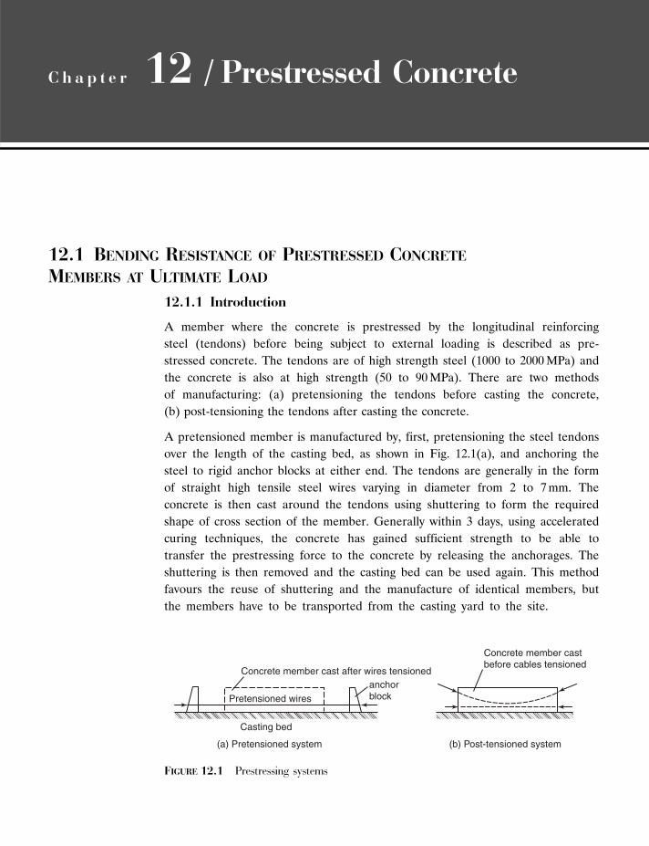
C h a p t e r 12 / Prestressed Concrete
12.1 BENDING RESISTANCE OF PRESTRESSED CONCRETE
MEMBERS AT ULTIMATE LOAD
12.1.1 Introduction
A member where the concrete is prestressed by the longitudinal reinforcing
steel (tendons) before being subject to external loading is described as pre-
stressed concrete. The tendons are of high strength steel (1000 to 2000 MPa) and
the concrete is also at high strength (50 to 90 MPa). There are two methods
of manufacturing: (a) pretensioning the tendons before casting the concrete,
(b) post-tensioning the tendons after casting the concrete.
A pretensioned member is manufactured by, first, pretensioning the steel tendons
over the length of the casting bed, as shown in Fig. 12.1(a), and anchoring the
steel to rigid anchor blocks at either end. The tendons are generally in the form
of straight high tensile steel wires varying in diameter from 2 to 7 mm. The
concrete is then cast around the tendons using shuttering to form the required
shape of cross section of the member. Generally within 3 days, using accelerated
curing techniques, the concrete has gained sufficient strength to be able to
transfer the prestressing force to the concrete by releasing the anchorages. The
shuttering is then removed and the casting bed can be used again. This method
favours the reuse of shuttering and the manufacture of identical members, but
the members have to be transported from the casting yard to the site.
Concrete member cast after wires tensioned
(a) Pretensioned system (b) Post-tensioned system
Casting bed
Pretensioned wiresanchorblock
Concrete member castbefore cables tensioned
FIGURE 12.1 Prestressing systems

A post-tensioned member is manufactured by first preparing the shuttering which
supports sheaths or ducts. The ducts contain unstressed tendons (see Fig. 12.1(b)) in
the form of straight or curved cables, or bars, which are free to move in the direction
of their length but are restrained to prevent movement transversely. The concrete
is then poured into the mould and allowed to gain strength. There is less urgency in
this method of manufacture and the shuttering is removed after a few days. Later,
when the concrete has matured the steel is stressed by jacking against the ends of
the beam and anchored using wedges for cables, or nuts on threaded rods for bars.
The method is suitable for members of different cross section and for members
which are cast in place on the construction sites where road access is difficult.
The advantages of prestressed concrete as compared with ordinary reinforced
concrete are:
(a) reduced self weight of members,
(b) no cracks at service load and consequently better durability,
(c) increased shear resistance.
The disadvantages of prestressed concrete as compared with ordinary reinforced
concrete are:
(a) increased cost of materials and shuttering,
(b) greater supervision required to ensure correct concrete strength and magnitude
of prestress forces,
(c) design calculations are more extensive.
12.1.2 Analysis of a Section in Bending at the Ultimate Limit State(cl 3.1.7, EN)
Analysis entails the determination of the moment of resistance of a section given
the size of the section and reinforcement. The behaviour of a prestressed concrete
member in bending at the ultimate limit state is similar to that of an ordinary
reinforced concrete member. The appearance of a beam element in bending is
shown in Fig. 12.2, where tensile cracks, commencing in the extreme tension fibres,
extend to the edge of the compression zone. The compressive force at the top of the
section is balanced by the tensile force in the steel at the bottom of the section.
In very simple terms the moment of resistance of a section in bending is therefore
the magnitude of the couple Cz or Tz.
The basic concepts are simple and the analysis of a section in bending at ultimate
load is based on the following assumptions (cl 3.1.7, EN).
(a) Plane sections remain plane,
(b) The strain in bonded reinforcement, whether in tension or compression, is
the same as that in the surrounding concrete.
322 � Chapter 12 / Prestressed Concrete

(c) The tensile strength of concrete is ignored.
(d) The stresses in the reinforcement or prestressing steel are derived from the
design curves (Fig. 3.10, EN).
(e) The initial prestrain in the prestressing tendons is taken into account when
assessing the stresses in the tendons at the ultimate limit state.
(f) For cross sections subject to pure longitudinal compression, the compressive
strain is limited to 0,002 and for bending 0,0035.
(g) The tensile strain in the steel is limited to 0,02.
Applying the assumptions listed above and assuming a rectangular stress block in
compression (Fig. 3.5, EN). The design resistance moment of a prestressed beam
containing bonded tendons at design strength, all of which are located in the
tension zone.
MRd ¼ ð fpk=�sÞApz ¼ fpd Apz ¼ fpd Apðd� lx=2Þ ð12:1Þ
where the factor defining the effective depth of the stress block (Eqs 3.19 and
3.20, EN)
l ¼ 0,8 for fck � 50 MPa
l ¼ 0,8 � ð fck � 50Þ=400 for 505fck � 90 MPa
The depth of the compression (x) is obtained by equating the force in the com-
pression zone to the balancing force in the tension zone
x=d ¼ fpd=ðl � fcdÞ ð12:2Þ
where the factor for defining the effective strength (Eqs 3.21 and 3.22, EN)
� ¼ 1,0 for fck � 50 MPa
� ¼ 1,0 � ð fck � 50Þ=200 for 505fck � 90 MPa
These equations assume that the steel and concrete reach their limiting values which
must be confirmed.
Compressionzone
M Mx
z
fp Ap
d
Strain
0,0035
lx
hfcd = hfck/gc
C
T
(a) (b) (c)
s
FIGURE 12.2 Bending resistance of a prestressed concrete beam at ultimate load
Concrete Design � 323

EXAMPLE 12.1 Analysis of a prestressed beam in bending at ultimate load.
Determine the ultimate moment of resistance for the prestressed beam section
shown in Fig. 12.3 from basic principles assuming bonded tendons.
From Eq. (12.2) for fck¼ 50 MPa and fpk¼ 1770 MPa, the ratio
x=d ¼ fpd=ðl� fcdÞ
¼ 846=ð400 � 600Þ � ð1770=1,15Þ=ð0,8 � 1,0 � 50=1,5Þ ¼ 0,203
Hence x¼ 0,203� 600¼ 122 mm which is less than the thickness of the 200 mm
top flange (Fig. 12.3), and is therefore satisfactory.
The moment of resistance of the section at the ultimate limit state
MRd ¼ fpdApðd� l x=2Þ
¼ ð1770=1,15Þ � 846 � ð600 � 0,4 � 0,203 � 600Þ=1E6 ¼ 717,8 kNm:
Check that the steel is at the ultimate design strength. For linear strain distribution
over the depth of the cross section the bending strain in the steel
"sb ¼ 0,0035ðd=x� 1Þ ¼ 0,0035 � ð600=122 � 1Þ ¼ 0,0137
For an initial stress of 0,75fpk in the steel and an estimated loss of prestress at service
load of 25 per cent
fpe=fpk ¼ 0,75 � 0,75 ¼ 0,563
Total strain in the steel is the sum of the bending and prestress strains ¼ "sb þ "sp ¼
"sb þ fpe=Es ¼ 0,0137 þ 0,563 � 1770=200E3 ¼ 0,0187:
If the steel is at the maximum design value of fpk/�s then from the stress–strain
relationship for steel the strain in the steel will be equal to, or greater than
fpd=Es ¼ ð1770=1,15Þ=200E3 ¼ 0,0077:
800
200
b = 400
fpk = 1700 MPa
Ap = 846 mm2
fck = 50 MPa
l = 20 m
d =
600
FIGURE 12.3 Example: analysis of a section inbending at ultimate load
324 � Chapter 12 / Prestressed Concrete
The total strain of 0,01874 0,0077, therefore the assumption that the steel is
at the maximum design stress of fpk/�s is justified. The total strain is also less than
the lim"ud¼ 0,02 (cl 3.3.6, EN).
12.1.3 Design of a Section in Bending at Ultimate Load
The design of a section in bending at ultimate load entails determining the size of
section and reinforcement given the magnitude of the bending moment. The design
can be carried out from first principles using the equations given in 12.1.2, but this
is tedious and can be avoided by using a graph (Annex B2). The design is based on
the rectangular concrete stress block in compression and is constructed as follows:
Moment of resistance related to the concrete compression zone
MRd ¼ fpd Apðd� l x=2Þ
This equation can be rearranged in non-dimensional form for the vertical axis of
the graph as
MRd=ðbd2fckÞ ¼ �ð fcd=fckÞl ðx=dÞð1 � lx=dÞ
Similarly equating the tensile force to the compression force the horizontal axis
of the graph
Apfpk=ðbd fckÞ ¼ �ð fpk=fpdÞð fcd=fckÞlðx=dÞ
A graph can be plotted by iterating values of (x/d) and checking for fpd5 yield
and "ud4 0,02 (cl 3.3.6, EN). A typical graph for fck¼ 50 MPa and fpk¼ 1170 MPa
is shown in Annex B2. Others are required for different concrete, steel strength
and material factors.
EXAMPLE 12.2 Design of a prestressed beam in bending at ultimate load.
Determine the size of a prestressed concrete section to support a uniformly
distributed design load of 125 kN at the ultimate limit state over a simply supported
span of 15 m. Assuming fpk¼ 1770 MPa, and Grade C50/60 concrete. Many similar
beams to be made and access to the sties is good therefore use pretensioned beams.
Design bending moment at ultimate load
MEd ¼ WL=8 ¼ 125 � 15=8 ¼ 234,4 kNm
The smallest depth of a simply supported beam, where deflection is not likely to
be a problem at service load, is approximately span/30. Try h¼ 15E3/30¼ 500 mm.
To optimize on the weight an ‘I’ cross section is generally used in prestressed
concrete but members should not be too slender because of instability. Assume
breadth b¼ 0,5 h¼ 250 mm. Web thickness is generally not less than 100 mm to resist
Concrete Design � 325

shear and should provide room for wires. Assume d¼ 425 mm (Fig. 12.4). Cover
should meet the requirements for durability and fire (Chapter 5).
Having decided on values of h, d and b calculate
MEd=ðbd2fckÞ ¼ 24,4E6=ð250 � 4252 � 50Þ ¼ 0,104
Assume fpe/fpk¼ 0,5. From a graph (Annex B2), Ap fpk/(bd fck)¼ 0,13 and hence
Aps ¼ 0,13 � 250 � 425 � 50=1770 ¼ 390 mm2, use 10�7 mm wires,
Aps ¼ 384; 8 mm2:
Minimum area of longitudinal steel (cl 9.2.1.1(1), EN)
As, min ¼ 0,26ð fcm=fykÞbtd ¼ 0,26 � ð4,1=1770Þ � 250 � 425
¼ 63,995Apsð384,8Þmm2, satisfactory
From a graph (Annex B2) x/d¼ 0,21 hence
x ¼ 0,21 � 425 ¼ 89,3 mm: Use top flange thickness of 150 mm:
The tension flange area must provide room for the wires with adequate spacing and
cover. Try all the wires on one row.
Width required¼ coverþ 9 spacesþ cover¼ 50þ 9� 50þ 50¼ 550 mm
This value is greater than the width of the section, therefore use two layers as shown
in Fig. 12.4.
Thickness of tension flange¼ coverþ spaceþ cover¼ 150 mm. Also make the com-
pression flange the same thickness to produce a symmetrical section which makes
Compressionflange
150
b = 250
h = 500d = 425
Tension flange
100
15050
50
40FIGURE 12.4 Example: design of asection in bending at ultimate load
326 � Chapter 12 / Prestressed Concrete

calculations easier at the service load conditions. The inside faces of the flanges
are generally sloped to aid in removing shuttering and to avoid cracks associated
with 908 angles.
12.2 BENDING RESISTANCE OF A PRESTRESSED CONCRETE BEAM
AT SERVICE LOAD
12.2.1 Introduction
Prestressed concrete members must satisfy two criteria at the serviceability limit
state in bending. The tensile stresses in the concrete must not produce cracks, except
in special circumstances, and the compressive stresses must not exceed the design
values. These two criteria of tensile stress and compressive stress form the basis
for analysis and design at the serviceability limit state in bending.
12.2.2 Analysis of a Section in Bending at the Serviceability Limit State
In Section 12.1.3 design formulae are developed with tensile and compressive
stress criteria, but because this is complicated it is initially instructive to analyse a
section in bending at the serviceability limit state and to identify the critical stresses.
EXAMPLE 12.3 Analysis of a section in bending at the serviceability limit state.
Determine the stresses due to prestress and applied service load for a beam of
uniform cross section shown in Fig. 12.5(a). The jacking force of 1600 kN is provided
by straight high tensile steel wires located as shown. The service load bending
moment, which includes the self-weight, is 550 kNm.
−9
−9 −15,79 −20,66
−16,5
+24,12
+1,5400
2001
2
(a) (b) (c)
100
Pt =1400kN
ft2 = +1,8 MPa
ft1 = −24,79 MPa fs1 = +3,46 MPa
fs2 = −15 MPa
e =
250
y =
475
Centroidal
Stresses at transfer after10% loss
Stresses at service load after25% loss
axis
200
400
800
200
+10,8
+ = + =
FIGURE 12.5 Example: analysis of a prestressed beam in bending at service load
Concrete Design � 327

If the section is not cracked and the compressive stresses are not greater than � fck/�c
then the elastic behaviour may be assumed. The percentage of steel is generally
small in relation to the concrete and therefore composite action is ignored.
The elastic section properties of the concrete are obtained as follows.
Cross-sectional area of the concrete
Ac ¼ ð80 þ 40 þ 40ÞE3 ¼ 160E3 mm2
Centroid of the cross section from moments of areas about the base
80E3 � 700 þ 40E3 � 400 þ 40E3 � 100 ¼ 160E3 � �yy
hence �yy ¼ 475 mm from the base.
Second moment of area of the cross section about the centroidal axis
I ¼ �ðbh3=3Þ
¼ ð400 � 3253 � 300 � 1253 þ 200 � 4753 � 100 � 2753Þ=3 ¼ 10,83E9 mm4
Elastic section moduli
Ze1 ¼ I=y1 ¼ 10,83E9=475 ¼ 22,80E6 mm3
Ze2 ¼ I=y2 ¼ 10,83E9=325 ¼ 33,32E6 mm3
The section properties are now used to determine the stresses in the extreme fibres
of the cross section. Subscript 1 denotes the bottom of the section and 2 the top of
the section. Compressive stresses are negative and tensile stresses are positive.
Critical stresses occur at transfer when the jacking force of 1600 kN is applied.
Loss of prestress of approximately 10 per cent occurs immediately because of the
elasticity of the concrete which reduces the length of the member. A more accurate
assessment of the loss is given in Section 12.3.
Prestressing force applied to the concrete at transfer Pt¼ 1400 kN.
Stress at the bottom of the section due to the prestressing force at transfer
ft1 ¼ �Pt=Ac � Pte=Ze1
¼ �1400E3=160E3 � 1400E3 � 250=22,80E6 ¼ �9 � 15,79 ¼ �24,79 MPa
Stress at the top of the section due to the prestressing force at transfer
ft2 ¼ �Pt=Ac þ Pte=Ze2
¼ �1400E3=160E3 þ 1400E3 � 250=33,32E6
¼ �9 þ 10,8 ¼ þ1,8 MPa
328 � Chapter 12 / Prestressed Concrete
The axial stresses can be added algebraically to the bending stresses because
the principal of superposition is valid for elastic behaviour. Diagrams can now be
drawn showing the stresses in the extreme fibres of the beam section at transfer
(Fig. 12.5(b)). The extreme fibre stresses can be joined by straight lines because they
vary linearly over the depth.
It is important to note that there is a tensile stress ofþ 1,8 MPa at the top of
the section and a compressive stress of � 24,79 MPa at the bottom of the section.
These stresses are critical and if they are too high in relation to the strength of the
concrete at that stage of loading, then cracking, or crushing, occurs. These stresses
occur at the supports for a straight member with a constant cross section and straight
wires. The stresses at the support for this type of beam are not modified by
the self-weight of the beam or the service load.
At midspan however the prestress stresses will be modified by the service load.
The critical stresses at the service load occur at midspan after further loss of
prestress due to creep in the steel and concrete occurs. The loss of prestress is
determined more accurately in Section 12.3, but at this stage it may be assumed that
the loss is 25 per cent of the jacking force.
Prestressing force at service load after losses, Ps ¼ 1200 kN.
The service load bending moment Ms, which includes self-weight, is 550 kNm. Stress
at the bottom of the section due to the prestressing force at service load and the
application of the service load bending moment
fs1 ¼ �Ps=Ac � Pse=Ze1 þMs=Ze1
¼ �1200E3=160E3 � 1200E3 � 250=22,80E6 þ 550E6=22,80E6
¼ �7,5 � 13,16 þ 24,12 ¼ þ3,46 MPa
Stress at the top of the section due to the prestressing force at service load and the
application of the service load bending moment
fs2 ¼ �Ps=Ac þ Pse=Ze2 �Ms=Ze2
¼ �1200E3=160E3 þ 1200E3 � 250=33,32E6 � 550E6=33,32E6
¼ �7,5 þ 9,0 � 16,50 ¼ �15,0 MPa:
These stresses can also be represented on diagrams as shown in Fig. 12.5(c). For
the service load condition it is important to notice that there is a tensile stress
ofþ3,46 MPa at the bottom of the section and a compressive stress of �15,0 MPa
at the top of the section. These stresses are critical and if they are too high in relation
to the strength of the concrete at this stage of loading then cracking, or crushing,
occurs.
Concrete Design � 329

The analysis of a beam is a good method for checking a section, but in practice
it is necessary to be able to determine the required size of a section to satisfy the
conditions at transfer and the serviceability limit state.
12.2.3 Design of a Section in Bending at the Serviceability Limit State
The critical bending stresses have been identified in the previous section and these
may be presented algebraically as follows.
The sign convention for stresses is negative compression and positive tension, with
the eccentricity positive below the centroidal axis and negative above. Subscript 1
denotes the bottom of the section and 2 the top of the section.
At transfer of the prestressing force Pt the stresses at the bottom and top of the
section
ft1 ¼ �Pt=Ac � Pte=Ze1 þMmin=Ze1 ð12:3Þ
ft2 ¼ �Pt=Ac þ Pte=Ze2 �Mmin=Ze2 ð12:4Þ
where Mmin is the bending moment that may act immediately the prestress is applied,
e.g. the self-weight bending moment.
Eqs (12.3) and (12.4) are applicable to a simply supported beam where the critical
section is at midspan e.g. the prestressing force is not parallel to the centroidal axis
of the section as shown in Fig. 12.6(a). However if the critical section is at the
support e.g. the prestressing force is parallel to the centroidal axis as shown in
Fig. 12.6(b), then the term containing Mmin is ignored.
Prestress force not parallel tothe centroidal axis
(a)
(b) Prestress force parallel tothe centroidal axis
FIGURE 12.6 Cable shapes for prestressed concrete beams
330 � Chapter 12 / Prestressed Concrete

After losses at the serviceability limit state the stresses at the bottom and top of the
section
fs1 ¼ �Ps=Ac � Pse=Ze1 þMs=Ze1 ð12:5Þ
fs2 ¼ �Ps=Ac þ Pse=Ze2 �Ms=Ze2 ð12:6Þ
where Ms is the service load bending moment and includes the minimum bending
moment Mmin.
If the extreme fibre stresses are now designated as serviceability design stresses
such that, ft1¼ ftc, ft2¼ ftt, fs1¼ fst, fs2¼ fsc, then combining Eqs (12.3) to (12.6) and
eliminating the eccentricity e, the optimum values of the section moduli can be
determined.
Combining Eqs (12.3) and (12.5)
Z0e1 ¼ ðMs � �MminÞ=ð fst � �ftcÞ ð12:7Þ
Combining Eqs (12.4) and (12.6)
Z0e2 ¼ ðMs � �MminÞ=ð� ftt � fscÞ ð12:8Þ
where
� ¼ Ps=Pt ¼ ðPs=PoÞ=ðPt=PoÞ ¼ �s=�t
These values of the section moduli are the minimum theoretical values and must
not be confused with the actual values which are written without the accent,
i.e. as Ze1 and Ze2. In the design process the actual values of the section moduli
are greater than the minimum values, and therefore it is impossible to satisfy all
the stress constraints simultaneously.
The minimum initial value of the jacking force Po(min) is obtained by satisfying
the tensile stress constraints ftt and fst, i.e. combining Eqs (12.4) and (12.5), and
dividing by �t.
PoðminÞ ¼ Acð fstZe1 þ � fttZe2 �Ms þ �MminÞ=½��sðZe1 þ Ze2Þ� ð12:9Þ
The maximum value of the eccentricity, emax is obtained by satisfying the tensile
stress constraints ftt and fst, i.e. combining Eqs (12.4) and (12.5)
emax ¼ Ze1Ze2ð fst � � fttÞ � �MminZe1 �MsZe2½ �=
Acð fstZe1 þ � fttZe2 �Ms þ �MminÞ½ �
ð12:10Þ
Concrete Design � 331

The maximum initial value of the jacking force Po(max) is obtained by satisfying the
compressive stress constraints ftc and fsc, i.e. combining Eqs (12.3) and (12.6) and
dividing by �t
PoðmaxÞ ¼ Acð fscZe2 þ � ftcZe1 þMs � �MminÞ=½��sðZe1 þ Ze2Þ� ð12:11Þ
The minimum value of the eccenticity emin is obtained by satisfying the compressive
stress constraints ftc and fsc, i.e. combining Eqs (12.3) and (12.6)
emin ¼ Ze1Ze2ð�fsc þ � ftcÞ � �MminZe2 �MsZe1½ �=
Acð fscZe2 þ � ftcZe1 þMs � �MminÞ½ �ð12:12Þ
For economy is steel reinforcement it would be ideal to adopt the minimum jacking
force and maximum eccentricity. However in design it is often not possible to
adopt the minimum value of the jacking force Po(min) because the force is expressed
in a discrete number of wires, or cables. Also the associated maximum value of
eccentricity emax may not be practical because it lies outside the section. In design
calculations therefore a practical magnitude of the practical jacking force, Pop,
is adopted expressed in number of wires, or cables, fully stressed to the design stress
such that
PoðmaxÞ4Pop4PoðminÞ
The eccentricity (e) which is consistent with the practical jacking force Pop is then
obtained from Eq. (12.13) which is a rearrangement of Eq. (12.5) and satisfies
the tensile stress constraint fst at service load.
e ¼ ðMs � Ze1fstÞ=ð�sPopÞ � Ze1=Ac ð12:13Þ
A practical value of the eccentricity ep is then calculated by trial and error such
that ep is approximately equal to e, and also
emax4ep4emin
If the critical values ftt, ftc, fst, fsc are related to the characteristic concrete strength
then Eqs (12.3) to (12.13) form the basis for a method of design.
In harsh environments where durability is a problem no tensile stress are recom-
mended. For normal use of prestressed concrete tensile stresses are accepted.
Cracking is accepted where corrosion or weathering is not a problem, for long span
beams where the self-weight is large and must be kept to a minimum, where deflec-
tions are not critical, or for temporary structures.
332 � Chapter 12 / Prestressed Concrete
EXAMPLE 12.4 Design of a section in bending at the serviceability limit state.
A beam is simply supported over a span of 15 m and supports an imposed service
load of 33 kN. The section shown in Fig. 12.4 is satisfactory at the ultimate limit
state in bending, check that it is suitable for service load conditions.
Estimate of self weight of member
Wsw ¼ 10L3 ¼ 10 � 153=1E3 ¼ 33,75 kN
Self-weight bending moment
Msw ¼ WswL=8 ¼ 33,75 � 15=8 ¼ 63,28 kNm
Imposed load bending moment
Mi ¼ WL=8 ¼ 33 � 15=8 ¼ 61,88 kNm
Total service load bending moment
Ms ¼ Msw þMi ¼ 63,28 þ 61,88 ¼ 125,2 kNm
The beam has straight wires and a constant cross section. The characteristic strength
for steel is 1570 MPa. Assume concrete Grade C30/40 at transfer and C40/50 after
28 days. Assume a jacking stress in a wire of 0,9fp0,1k, a loss of prestress of 10
per cent at transfer and 25 per cent at service load. Consequently �t¼ 0,8, �s¼ 0,75
and �¼ �s/�t¼ 0,75/0,8¼ 0,938. Maximum compressive stress 0,45fck and maximum
tensile stress 0,3fck2/3.
The design stresses are (tension þve, compression �ve)
ftc ¼ 0,45 � ð�30Þ ¼ �13,5 MPa
ftt ¼ þ0,3 � 302=3 ¼ þ2,90 MPa
fst ¼ þ0,3 � 402=3 ¼ þ3,51 MPa
fsc ¼ 0,45 � ð�40Þ ¼ �18,0 MPa
Theoretical optimum design values of the section moduli from Eqs (12.7) and (12.8)
Z0e1 ¼ ðMs � �MminÞ=ð fst � � ftcÞ
¼ ð125,16E6 � 0Þ=½3,51 � ð0,938 ��13,5Þ� ¼ 7,74E6 mm3
Z0e2 ¼ ðMs � �MminÞ=ð� ftt � fscÞ
¼ ð125,16E6 � 0Þ=½0,938 � 2,9 � ð�18Þ� ¼ 6,04E6 mm3
The value of Mmin is zero because the prestressing force is parallel to the centroidal
axis of the section and consequently the critical section is at the support.
Concrete Design � 333
Actual second moment of area for the section (Fig. 12.4)
I ¼ �bh3=12 ¼ 250 � 5003=12 � 150 � 2003=12 ¼ 2,504E9 mm4
Actual section moduli
Ze1 ¼ Ze2 ¼ I=y ¼ 2,504E9=250 ¼ 10,02E6 mm3
The actual values of Ze4Z0e which is satisfactory but conservative. The size of the
section could be reduced based on these calculations, but the estimated total loss
of prestress may be greater than 25 per cent and this would increase the values of Z0e.
The section must also satisfy deflection and ultimate load restraints.
The values of Z0e also show that the optimum section is not symmetrical about
the horizontal centroidal axis and ideally it should be closer to the bottom of the
section. The reason for this is that the strength of the concrete at transfer is not
as great as at service load conditions. If self-weight of the member is important, or
if a very large number of members are to be made, then an iterative process is
carried out to reduce the self-weight of the section. However, the more complicated
the cross section the more costly the shuttering, but this can be justified if there
are large numbers to be manufactured.
Values of the prestressing force and eccentricity at transfer are obtained from
Eqs (12.9) to (12.12). Note that in the following calculations actual values of section
moduli are used, i.e. Ze1¼Ze2¼ 10,016E6 mm3.
Cross-sectional area (Fig. 12.4)
Ac ¼ 250 � 500 � 150 � 200 ¼ 95E3 mm2
Maximum value of the eccentricity for minimum jacking force, Eq. (12.10)
emax ¼ Ze1Ze2ð fst � � fttÞ � �MminZe1 �MsZe2½ �= Acð fstZe1 þ � fttZe2 �Ms þ �MminÞ½ �
¼ ½10,02E6 � 10,02E6 � ð3,51 � 0,938 � 2,9Þ � 0 � 125,2E6 � 10,02E6�=
½95E3 � ð3,51 � 10,02E6 þ 0,938 � 2,9 � 10,02E6 � 125,2E6 þ 0Þ�
¼ þ196,7 mm
Minimum value of the eccentricity for maximum jacking force, Eq. (12.12)
emin ¼ Ze1Ze2½�fsc þ � ftc� � �MminZe2 �MsZe1
� =
Ac½fscZe2 þ �ftcZe1 þMs � �Mmin��
¼ f10,02E6 � 10,02E6 � ½�18 þ 0,938 � ð�13,5Þ� � 0 � 125,2E6 � 10,02E6g=
95E3 � ½ð�18Þ � 10,02E6 þ 0,938 � ð�13,5Þ � 10,02E6 þ 125,2E6 � 0��
¼ þ41,5 mm:
334 � Chapter 12 / Prestressed Concrete

Maximum value of the prestressing force before losses for minimum eccentricity,
Eq. (12.11)
PoðmaxÞ ¼ Acð fscZe2 þ �ftcZe1 þMs � �MminÞ=½��sðZe1 þ Ze2Þ�
¼ 95E3 � ð�18Þ � 10,02E6 þ 0,938 � ð�13,5Þ � 10,02E6 þ 125,2E6 � 0�=½
½�0,75 � ð10,02E6 þ 10,02E6Þ� ¼ 1150 kN:
Minimum value of the jacking force before losses for maximum eccentricity from
Eq. (12.9)
PoðminÞ ¼ Acð fstZe1 þ � fttZe2 �Ms þ �MminÞ=½��sðZe1 þ Ze2Þ�
¼ 95E3 � 3,51 � 10,02E6 þ 0,938 � 2,9 � 10,02E6 þ 125,2E6 � 0�=½
½�0,75 � ð10,02E6 þ 10,02E6Þ� ¼ 397 kN:
The different values of the jacking force and eccentricity show that more than
one solution is possible. This is because the actual section moduli, Ze1¼Ze2¼
10,02E6 mm3, are greater than the optimum values Z0e1 ¼ 7,74E6 mm3 and
Z0e2 ¼ 6,04E6 mm3.
A practical value of the prestressing force Pop is now chosen such that
PoðmaxÞð1150Þ4Pop4PoðminÞð397Þ kN:
Practically the number (nw) of 7 mm diameter wires of jacking force
Pw ¼ �2=4 � 0,9fp0,1k ¼ � 72=4 � 0,9 � 1570=1E3 ¼ 54,4 kN:
PoðmaxÞ=Pw4nw4PoðminÞ=Pw
1150=54,44nw4397=54,4
21,14nw47,3
The wires are required at ultimate load (Fig. 12.4) and two wires at the top of
the section to prevent bending failure if the beam is inadvertently turned upside
down. The two top wires are also useful for fixing shear reinforcement.
Pop ¼ nwPw ¼ 12 � 42,3 ¼ 652,8 kN
If Pop¼ 652,8 kN then the corresponding eccentricity from Eq. (12.13)
e ¼ ðMs � Ze1fstÞ=ð�sPopÞ � Ze1=Ac
¼ ð125,2E6 � 10,02E6 � 3,51Þ=ð0,75 � 652,8E3Þ � 10,02E6=95E3 ¼ 78,4 mm:
Concrete Design � 335
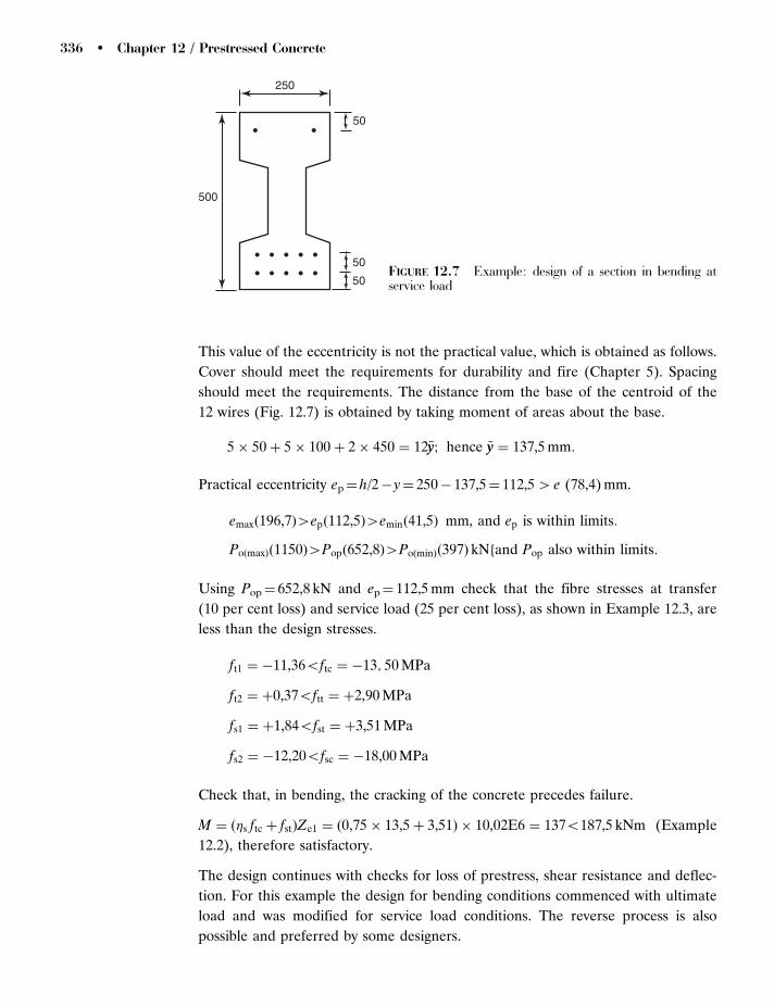
This value of the eccentricity is not the practical value, which is obtained as follows.
Cover should meet the requirements for durability and fire (Chapter 5). Spacing
should meet the requirements. The distance from the base of the centroid of the
12 wires (Fig. 12.7) is obtained by taking moment of areas about the base.
5 � 50 þ 5 � 100 þ 2 � 450 ¼ 12�yy; hence �yy ¼ 137,5 mm:
Practical eccentricity ep¼ h/2� y¼ 250� 137,5¼ 112,54 e (78,4) mm.
emaxð196,7Þ4epð112,5Þ4eminð41,5Þ mm, and ep is within limits:
PoðmaxÞð1150Þ4Popð652,8Þ4PoðminÞð397Þ kNfand Pop also within limits:
Using Pop¼ 652,8 kN and ep¼ 112,5 mm check that the fibre stresses at transfer
(10 per cent loss) and service load (25 per cent loss), as shown in Example 12.3, are
less than the design stresses.
ft1 ¼ �11,365ftc ¼ �13; 50 MPa
ft2 ¼ þ0,375ftt ¼ þ2,90 MPa
fs1 ¼ þ1,845fst ¼ þ3,51 MPa
fs2 ¼ �12,205fsc ¼ �18,00 MPa
Check that, in bending, the cracking of the concrete precedes failure.
M ¼ ð�s ftc þ fstÞZe1 ¼ ð0,75 � 13,5 þ 3,51Þ � 10,02E6 ¼ 1375187,5 kNm (Example
12.2), therefore satisfactory.
The design continues with checks for loss of prestress, shear resistance and deflec-
tion. For this example the design for bending conditions commenced with ultimate
load and was modified for service load conditions. The reverse process is also
possible and preferred by some designers.
50
50
500
250
50
FIGURE 12.7 Example: design of a section in bending atservice load
336 � Chapter 12 / Prestressed Concrete

12.2.4 Deflection Limits for Prestressed Concrete Members(cl 7.4, EN)
No definite limits are set for the deflections for prestressed concrete but as with
ordinary reinforced concrete the deformations of the structure, or part of it, should
not adversely affect its efficiency of appearance. Deflections should be compatible
with the degree of movement acceptable by other elements including finishes,
services, partitions, glazing and cladding.
The span/effective depth ratios for ordinary reinforced concrete are not appli-
cable to prestressed concrete because generally at service load the concrete
is not cracked, and also the prestressing force produces an upward camber of
the member. The deflections in prestressed concrete members may be described
as short term elastic deflections which occur immediately, and long term creep
and shrinkage deflections which occur after the member has been loaded for a
long time.
As a guide maximum downward and upward deflections should not exceed span/250.
This limit may cause excessive damage to contiguous elements, e.g. partitions, and
the limit is reduced to span/500 (cl 7.4.1, EN).
12.2.5 Short Term Elastic Deflections
These occur immediately when the prestressing force is applied at transfer, when
the self-weight and dead load act, and when the imposed load is applied. The
deflection due to the imposed load becomes zero when the imposed load is removed,
but the dead load and prestress deflections remain.
The elastic deformation for a beam of uniform section
ae ¼ ðL2=EcmðtÞÞ�kM ð12:14Þ
where
M is the maximum bending moment in the spank is a factor which depends on the shape of the bending moment diagram as shown
in Table 12.1Ecm(t) is the modulus of elasticity (cl 3.1.3, EN) for a particular concrete strength
derived from Ecm¼ 22(( fckþ 8)/10)0,3.
12.2.6 Long Term Creep Deflections
These are due to creep in the concrete which is dependent on the stress level and
the maturity of the concrete. The creep effect due to transient loads is very small
Concrete Design � 337

and only permanent loads need be considered, i.e. the dead load and permanent
imposed load.
Long term deflections can be calculated using an elastic analysis encorporating
the secant modulus of elasticity of the concrete (Ecm(t)) related to the elastic
modulus (Eq. 3.5, EN)
EcmðtÞ ¼ ð fcmðtÞ=fcmÞ0,3Ecm ð12:15Þ
where
fcm ¼ fck þ 8 MPa
EXAMPLE 12.5 Deflection of a prestressed beam.
Calculate the deflection of the simply supported prestressed beam which spans 15 m
designed in Example 12.4. Relevant details are I¼ 2,504E9 mm4, fck(3) ¼ 30,
fck(28)¼ 40 MPa, Pop¼ 652,8 kN, and ep ¼ 112,5 mm.
The calculated deflections which occur during the manufacture and loading of the
beam are as follows. Downwards deflections are postive.
TABLE 12.1 Deflection factors.
Load
w / unit length wL2 / 8
wL / 4
−Pe
P
P
Parabolic tendon
P
Pe
e
−Pe
L / 2 L / 2
548
112
18
5 48
Bending moment diagram k
L
W
338 � Chapter 12 / Prestressed Concrete
Deflections at transfer
Elastic modulus at 3 days (Table 3.1, EN)
Ecmð3Þ ¼ 22ðð fck þ 8Þ=10Þ0,3¼ 22 � ðð30 þ 8Þ=10Þ0,3
¼ 32,8 GPa
Elastic modulus at 28 days
Ecmð28Þ ¼ 22ðð fck þ 8Þ=10Þ0,3¼ 22 � ðð40 þ 8Þ=10Þ0,3
¼ 35,2 GPa
Elastic deflection (upwards) due to prestress at transfer at three days after 10
per cent loss.
ae ¼ L2=ðEcmð3ÞlÞ�kM ¼ L2=ðEcmð3ÞlÞð1=8Þð��tPopepÞ
¼ 15E32=ð32,8E3 � 2,504E9Þ � ð1=8Þ � ð � 0,8 � 652,8E3 � 112,5Þ
¼ �20,2 mm ðupwardsÞ:
Elastic deflection (downwards) from self-weight (33,75 kN) at transfer when the
beam is lifted from the casting bed
ae ¼ L2=ðEcmð3ÞlÞ�kM ¼ L2=ðEcmð3ÞlÞð5=48ÞðWL=8Þ
¼ 15E32=ð32,8E3 � 2,504E9Þ � ð5=48Þ � ð33,75E3 � 15E3=8Þ
¼ 18,0 mm ðdownwardsÞ
The net deflection at transfer (3 days)¼� 20,2þ 18,0¼� 2,2 mm (upwards). This
value is of interest but generally of little practical importance.
Long term deflections (cl 7.4.3(5), EN) Effective creep modulus of elasticity
related to the 3 day concrete strength. National size of section
¼ 2Ac=u ¼ 2 � ð500 � 250 � 200 � 150Þ=½2 � ð500 þ 250 þ 150Þ� ¼ 106 mm
Ec,eff ¼ Ecmð3Þ=ð1 þ �ð�,3ÞÞ ¼ 32,8E3=ð1 þ 3,3Þ ¼ 7,63 GPa
Final creep coefficient �(�,3)¼ 3,3 is interpolated from Fig. 3.1, EN for humid
outside conditions.
Long term creep deflection due to eccentricity of prestress after 25 per cent loss
ac ¼ L2=ðEc,eff lÞ�kM ¼ ðL2=Ec,eff lÞð1=8Þð��sPopepÞ
¼ 15E32=ð7,63E3 � 2,504E9Þ � ð1=8Þ � ð � 0,75 � 652,8E3 � 112,5Þ
¼ �81,2 mm ðupwardsÞ
Concrete Design � 339

Long term creep deflection due to self-weight (33,75 kN) bending
ac ¼ L2=ðEc,eff lÞ�kM ¼ L2=ðEc,eff lÞð5=48ÞðWL=8Þ
¼ 15E32=ð7,63E3 � 2,504E9Þ � ð5=48Þ � ð33,75E3 � 15E3=8Þ
¼ 77,6 mm ðdownwardsÞ:
Short term deflections Elastic deflection (downwards) from imposed load (33 kN)
related to the 28 day concrete strength
ae ¼ L2=ðEcmð28ÞlÞ�kM ¼ L2=ðEcmð28ÞlÞð5=48ÞðWL=8Þ
¼ 15E32=ð35,2E3 � 2,504E9Þ � ð5=48Þ � ð33E3 � 15E3=8Þ
¼ 16,4 mm ðdownwardsÞ
Net long term creep deflection¼� 81,2þ 77,6¼� 3,6 mm (upwards).
Short term elastic deflection from imposed load¼þ 16,4 mm (downwards).
As a guide if these deflections are compared with span/250¼ 15E3/500¼ 60 mm
then the previous calculations are within this limit. The limit of span/500¼ 15E3/
500¼ 30 mm, which is to prevent damage to partitions, is also satisfied.
12.3 LOSS OF PRESTRESS (cl 5.10, EN)12.3.1 Introduction
Loss of prestresses is the difference between the jacking force in the tendon at the
prestressing stage and the force after losses have occurred. Some of the losses occur
immediately when the force is transferred to the concrete, e.g. elastic shortening of
the member. Other losses occur with time, e.g. creep of the concrete. The jacking
force does not exceed 90 per cent of the characteristic strength of the tendon and
is generally not less than 75 per cent (cl 5.10.3(2), EN). In practice total losses of
the jacking force are within the range of 15 to 40 per cent. If large losses of prestress
occur then the advantages of prestressed concrete, e.g. no cracks at service load, are
lost. It is therefore advantageous to minimize the loss of prestress.
Losses of prestress are related to the jacking stress and expressed as: per cent loss of
prestress¼ 100 (jacking stress� final stress)/(jacking stress)
In general, losses can occur because of shortening of the concrete member, or
shortening of the tendon or because of friction acting along the length of the tendon.
The following factors affect the loss of prestress:
(a) relaxation of the steel (1�12%),
(b) elastic deformation of the concrete (1�10%),
340 � Chapter 12 / Prestressed Concrete
(c) shrinkage of the concrete (1�6%),
(d) creep of the concrete (5�15%),
(e) draw-in during anchorage (0�5%),
(f) friction in the ducts and at anchorages (3�7%).
The previous list considers each less separately but an alternative is to use Eq. 5.46,
EN which calculates time dependent losses in a single formula.
Initially, in design calculations, the loss of prestress is estimated from past
experience and later, when the section shape and size has been determined, a more
accurate calculation is made. A reasonably accurate estimation of the loss of pre-
stress is required because it affects service load conditions, e.g. the bending moment
at which bending cracks occur and also the shear force at which diagonal shear
cracks appear.
12.3.2 Relaxation of Steel (cl 5.10.4, EN)
If a steel tendon is stressed to 80 per cent of its characteristic strength and anchored
over a fixed length, then after 1000 h the stress will reduce. This phenomena, which
is not fully understood, is called relaxation, and may be defined as a loss of stress
at constant strain. In prestressed concrete the fixed length is the concrete member,
although in reality this does change slightly.
For design calculations the value adopted for the loss should be the 1000 h relaxa-
tion value taken from certificates accompanying the consignment.
12.3.3 Elastic Deformation of the Concrete (cl 5.10.4, EN)
If a jacking force from a prestressing tendon is transferred to a concrete member
then, because the concrete behaves elastically, the member immediately reduces in
length. If the steel and concrete are bonded together, as in pretensioned prestressed
concrete, then the reduction in length is the same for the concrete and the steel
and is unavoidable. In post-tensioned concrete, because the tendon is not bonded
to the concrete during stressing operations, the elastic reduction in length of the
concrete can be allowed for when jacking and the loss can be reduced to a very
small value.
The simplest method of calculating the loss of prestress due to elastic
shortening is as follows. Assuming elastic behaviour for a pretensioned
member where the steel is bonded to the concrete before the jacking force is
transferred to the concrete. If f 0s is the loss of stress in the steel and fc is the stress
Concrete Design � 341

in the concrete adjacent to the steel at transfer strain in the concrete¼ strain in
the steel
cp=Ec ¼ f 0s=Es
Percentage loss of prestress, if fpi is the jacking stress in the steel
¼ 100ð f 0s=fpiÞ ¼ 100ðEs=EcÞcp=fpi ð12:16Þ
Modulus of elasticity (cl 3.1.3, EN)
Ecm ¼ 22ðð fck þ 8Þ=10Þ0,3 GPa
where fck in MPa is the strength of the concrete at transfer.
The value of the modulus of elasticity for wires and bars is 200 GPa and for strand
190 GPa (cl 3.3.6(3), EN).
Eq. (12.16) can also be applied to a post-tensioned beam but if the elastic shorten-
ing is allowed for in the jacking process then the loss will be very small. Losses for
elastic shortening can therefore vary between 1 per cent for some post-tensioned
beams and 10 per cent for highly prestressed pretensioned members.
12.3.4 Shrinkage of Concrete (cl 3.1.4, EN)
Shrinkage of concrete is a reduction in dimensions of a concrete member and
when related to loss of prestress it is the shrinkage in length which is important.
The more important factors which influence shrinkage in concrete are:
(a) aggregate used,
(b) original water content,
(c) effective age at transfer,
(d) effective section thickness,
(e) ambient relative humidity.
In the absence of experimental evidence values of shrinkage strain ("c) are given in
Table 3.2, EN. These values are incorporated in the following theory. Assuming
elastic behaviour the loss of prestress in the prestressing steel
fs ¼ Es"s
Assuming equal strains in the steel and concrete
"s ¼ "c
and the percentage loss of prestress related to the jacking stress
¼ 100ð fs=fpiÞ ¼ 100Es"c=fpi ð12:17Þ
342 � Chapter 12 / Prestressed Concrete

12.3.5 Creep of Concrete (cl 3.1.4, EN)
Creep is the change in strain which occurs very slowly after the immediate elastic
strain has taken place. The creep coefficient depends on the following:
(a) original water content,
(b) effective age at transfer,
(c) effective section thickness,
(d) ambient relative humidity,
(e) ambient temperature.
Creep strain in concrete is stress dependent and values are obtained from Fig. 3.1,
EN. Expressed as the elastic strain multiplied by the final creep coefficient �4 1
"ccð�,toÞ ¼ ðc=EcÞ�ð�,toÞ
Assuming elastic behaviour, then loss of prestress in the steel
fs ¼ Es"s
Assuming the strain in the steel equals the creep strain in the concrete
"s ¼ "ccð�,toÞ ¼ ðc=EcÞ�ð�,toÞ
and the percentage loss of prestress related to the jacking stress
¼ 100ð fs=fpiÞ ¼ 100ðEs=EcÞ�ð�,toÞc=fpi ð12:18Þ
12.3.6 Anchorage Slip (cl 5.10.4, EN)
Anchorage slip reduces the stress in the wires or tendon and results in a loss of
prestress.
When the wires for pretensioned prestressed concrete members are being stressed
the wires are fixed to a single cross-head and the slip can be allowed for and
consequently the loss of prestress is small.
In post-tensioning systems allowance should be made for any slip of the
tendon at the anchorage when the prestressing force is transferred from the
tensioning equipment to the anchorage. This loss may be large for short members.
In practice the slip at the anchorage @L is known and the strain @L=L can be
calculated.
Percentage loss of prestress related to the jacking stress
¼ 100ð fs=fpiÞ ¼ 100ð@L=LÞEs=fpi ð12:19Þ
Concrete Design � 343
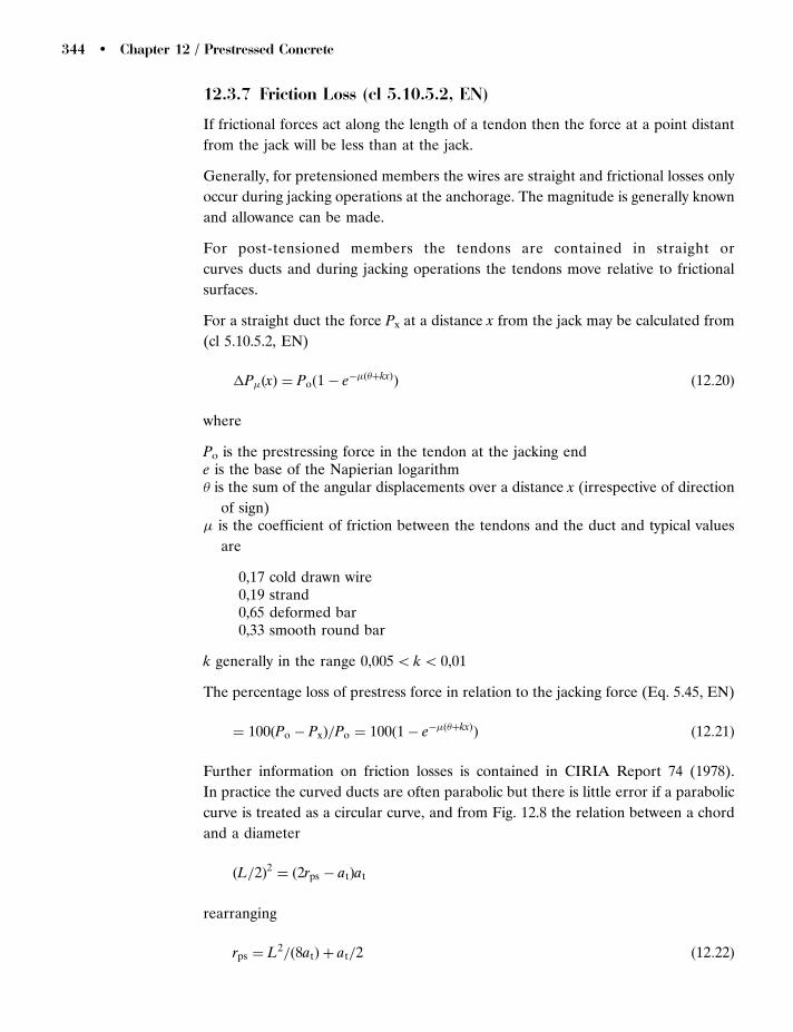
12.3.7 Friction Loss (cl 5.10.5.2, EN)
If frictional forces act along the length of a tendon then the force at a point distant
from the jack will be less than at the jack.
Generally, for pretensioned members the wires are straight and frictional losses only
occur during jacking operations at the anchorage. The magnitude is generally known
and allowance can be made.
For post-tensioned members the tendons are contained in straight or
curves ducts and during jacking operations the tendons move relative to frictional
surfaces.
For a straight duct the force Px at a distance x from the jack may be calculated from
(cl 5.10.5.2, EN)
�P�ðxÞ ¼ Poð1 � e��ð�þkxÞÞ ð12:20Þ
where
Po is the prestressing force in the tendon at the jacking ende is the base of the Napierian logarithm� is the sum of the angular displacements over a distance x (irrespective of direction
of sign)� is the coefficient of friction between the tendons and the duct and typical values
are
0,17 cold drawn wire0,19 strand0,65 deformed bar0,33 smooth round bar
k generally in the range 0,0055 k5 0,01
The percentage loss of prestress force in relation to the jacking force (Eq. 5.45, EN)
¼ 100ðPo � PxÞ=Po ¼ 100ð1 � e��ð�þkxÞÞ ð12:21Þ
Further information on friction losses is contained in CIRIA Report 74 (1978).
In practice the curved ducts are often parabolic but there is little error if a parabolic
curve is treated as a circular curve, and from Fig. 12.8 the relation between a chord
and a diameter
ðL=2Þ2 ¼ ð2rps � atÞat
rearranging
rps ¼ L2=ð8atÞ þ at=2 ð12:22Þ
344 � Chapter 12 / Prestressed Concrete
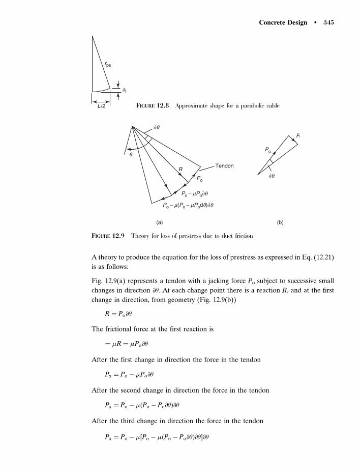
A theory to produce the equation for the loss of prestress as expressed in Eq. (12.21)
is as follows:
Fig. 12.9(a) represents a tendon with a jacking force Po subject to successive small
changes in direction @�. At each change point there is a reaction R, and at the first
change in direction, from geometry (Fig. 12.9(b))
R ¼ Po@�
The frictional force at the first reaction is
¼ �R ¼ �Po@�
After the first change in direction the force in the tendon
Px ¼ Po � �Po@�
After the second change in direction the force in the tendon
Px ¼ Po � �ðPo � Po@�Þ@�
After the third change in direction the force in the tendon
Px ¼ Po � �½Po � �ðPo � Po@�Þ@��@�
at
rps
L /2 FIGURE 12.8 Approximate shape for a parabolic cable
Tendon
(a) (b)
R
R
Po
Po − mPo∂q
Po − m(Po − mPodq)∂q
Po
∂q
∂q
q
FIGURE 12.9 Theory for loss of prestress due to duct friction
Concrete Design � 345
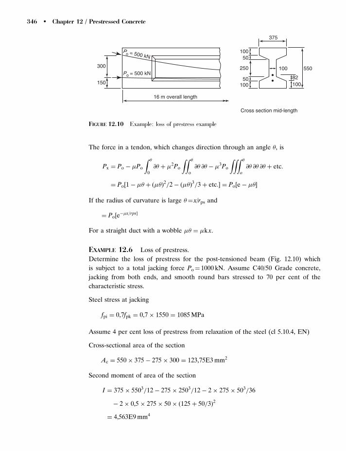
The force in a tendon, which changes direction through an angle �, is
Px ¼ Po � �Po
Z �
0
@� þ �2Po
ZZ �
o
@� @� � �3Po
ZZZ �
o
@� @� @� þ etc:
¼ Po½1 � �� þ ð��Þ2=2 � ð��Þ3=3 þ etc:� ¼ Po½e � ���
If the radius of curvature is large �¼ x/rps and
¼ Po½e��x=rps�
For a straight duct with a wobble �� ¼ �k x.
EXAMPLE 12.6 Loss of prestress.
Determine the loss of prestress for the post-tensioned beam (Fig. 12.10) which
is subject to a total jacking force Po¼ 1000 kN. Assume C40/50 Grade concrete,
jacking from both ends, and smooth round bars stressed to 70 per cent of the
characteristic stress.
Steel stress at jacking
fpi ¼ 0,7fpk ¼ 0,7 � 1550 ¼ 1085 MPa
Assume 4 per cent loss of prestress from relaxation of the steel (cl 5.10.4, EN)
Cross-sectional area of the section
Ac ¼ 550 � 375 � 275 � 300 ¼ 123,75E3 mm2
Second moment of area of the section
I ¼ 375 � 5503=12 � 275 � 2503=12 � 2 � 275 � 503=36
� 2 � 0,5 � 275 � 50 � ð125 þ 50=3Þ2
¼ 4,563E9 mm4
16 m overall length
Cross section mid-length
10050
250
50100
375
100 550
10082
300
Po = 500 kN
Po = 500 kN
150
FIGURE 12.10 Example: loss of prestress example
346 � Chapter 12 / Prestressed Concrete

Elastic section modulus of the section
Z ¼ I=y ¼ 4,563E9=275 ¼ 16,594E6 mm3
Prestress at the centroid of the prestressing steel
c ¼ �Po=Ac � Poey=I
¼ �1000E3=123,75E3 � 1000E3 � 134 2=4,563E9 ¼ �12,0 MPa
Elastic modulus of the concrete at 28 days (cl 3.1.3, EN)
Ecmð28Þ ¼ 22 � ðð fckð28Þ þ 8Þ=10Þ0,3¼ 22ðð40 þ 8Þ=10Þ0,3
¼ 35,2 GPa
Elastic modulus at transfer at three days
Ecmð3Þ ¼ 22 � ðð fckð3Þ þ 8Þ=10Þ0,3¼ 22ðð25 þ 8Þ=10Þ0,3
¼ 31,5 GPa
Percentage loss of prestress from elastic deformation of the concrete from
Eq. (12.16)
¼ 100ðEs=Ecmð3ÞÞcp=fpi ¼ 100 � ð200E3=31,5E3Þ � 12=1085 ¼ 7,02%
This value can be halved to 3,51 per cent for a post-tensioned beam.
Percentage loss of prestress from drying shrinkage of the concrete (Table 3.2, EN)
from Eq. (12.17) for outdoor conditions 80 per cent humidity (2Ac/u¼ 111 mm)
¼ 100Es"cd=fpi ¼ 100 � 200E3 � 310E � 6=1085 ¼ 5,71%
Percentage loss of prestress from creep of the concrete (Section 2.6.2), transfer at
3 days for outdoor exposure (Fig. 3.1, EN). From Eq. (12.18)
¼ 100ðEs=Ecmð3ÞÞ�c=fpi ¼ 100 � ð200E3=31,5E3Þ � 2,5 � 12=1085 ¼ 17,56%
Percentage loss of prestress from slip of 1 mm for half the length of beam during
anchorage from Eq. (12.19)
¼ 100ð@L=LÞEs=fpi ¼ 100 � ð1=8E3Þ � 200E3=1085 ¼ 2,30%
Radius of curvature for bottom cable from Eq. (12.23) assuming the curve approx-
imates to a circle (at¼ 150� 100¼ 50 mm)
rps ¼ L2=ð8atÞ þ at=2 ¼ 162=ð8 � 0,05Þ þ 0,05=2 ¼ 640 m
Percentage loss of prestress from friction for the bottom approximately straight
duct (cl 5.10.5.2, EN) jacked from both ends from Eq. (12.21)
¼ 100ð1 � e��ð�þkxÞÞ ¼ 100 � ð1 � e�0,25�ð8=640þ0,0075�8ÞÞ ¼ 1,79%
Concrete Design � 347

Radius of curvature for the top curved duct from Eq. (12.22) assuming the curve
approximates to a circle (at¼ 450� 182¼ 268 mm)
rps ¼ L2=ð8atÞ þ at=2 ¼ 162=ð8 � 0,268Þ þ 0,268=2 ¼ 119,5 m
Percentage loss of prestress from friction for top cable jacked from both ends from
Eq. (12.21)
¼ 100ð1 � e��ð�þk xÞÞ ¼ 100 � ð1 � e�0,25�ð8=119,5þ 0,0075�8ÞÞ ¼ 3,12%
Total loss of prestress
¼ relax:þ elastic conc:þ shrink conc:þ creep conc:þ slip þ friction
¼ 4 þ 3,51 þ 5,71 þ 17,56 þ 2,3 þ ð1,79 þ 3,12Þ=2 ¼ 35,5%
The total loss can be reduced by rejacking to reduce the concrete elastic loss,
or increasing the concrete strength.
The European Code gives an alternative method of calculating the time-dependent
losses (cl 5.10.6, EN). These include shrinkage of concrete, relaxation of the steel
and creep of concrete. Loss of stress in the tendons
�p,cþ sþ r ¼ ð"csEp þ 0,8�pr þ Ep=Ecm�ðt,toÞc,QPÞ=
ð1 þ Ep=EcmAp=Acð1 þ Ac=Iz2cpÞð1 þ 0,8�ðt,toÞÞ
�p,cþsþr ¼ ð310=1E6 � 200E3 þ 0,8 � 0,04 � 1085 þ 200E3=35E3 � 2,5 � 12Þ=
ð1 þ 200E3=35E3 � 645,3=123,75E3ð1 þ 123,75E3=4563E9 � 1342Þ
� ð1 þ 0,8 � 2,5Þ
¼ ð62 þ 34,72 þ 171,4Þ=ð1 þ 0,0298ð1 þ 0,487Þ � 3Þ ¼ 236,7 MPa:
Percentage loss¼ 236,7/1085� 100¼ 21,8
Compare with previous calculation, per cent loss¼ 4þ 5,71þ 17,56¼ 27,274 21,8.
12.4 ANCHORAGE OF TENDONS
12.4.1 Anchorage for Post-tensioned Tendons (cl 8.10.3, EN)
When a force from a post-tensioned cable is transferred to a small area, or zone,
at the end of a beam, high localized stresses are produced. These localized stresses
do not extend the full length of the member but are confined to the anchor
block. The tensile stresses are of particular concern because they can produce
cracks in the concrete which need to be controlled by the use of reinforcing steel.
348 � Chapter 12 / Prestressed Concrete

The cross section of the another blocks is generally rectangular in order to reduce
the magnitude of the stresses.
The exact distribution of stresses in an anchor block is complex and is not fully
understood theoretically nor has the subject been thoroughly investigated experi-
mentally (CIRIA Guide 1, 1976). The distribution of principal compressive and
tensile stresses in a simple rectangular anchor block subject to a single force
are shown in Fig. 12.11(a). The distribution of stress along the centre line of the
block is shown in Fig. 12.11(b), and this is of particular concern in structural design
because reinforcement is required to resist the tensile stresses. These stresses are
three-dimensional and consequently tensile stresses are also present at right angles
to those shown in Fig. 12.11(b).
In addition to the stresses described previously, where there is more than one jacking
force there are stresses close to the loaded face which may cause cracking and
spalling of the surface concrete between the anchor forces. These spalling stresses
are greatest with unsymmetrical loading of the end block.
When several forces are applied to an end block similar distribution to those
described for a single force occur local to each force, and also over the complete
end block. It is this fact which is used in design calculations to simplify a complex
problem by subdividing the complete end block into simple individual cubic
end blocks associated with each anchor force. Examples are shown in Fig. 12.12.
The size of each individual cubic end block is based on a controlling dimension yo
Tensile
Tension
PCL
Compressive
Compression
0,2y0 2y0
(a) Simplified stress trajectories
(b) Distribution of stress along CL of blockFIGURE 12.11 Stress distribution in a post-tensioned end block
Concrete Design � 349

which may be a vertical edge distance as in Fig. 12.12(a), or a horizontal edge
distance as in Fig. 12.12(b), or distance between anchor forces as in Fig. 12.12(c).
The minimum dimension is then used to determine the minimum size of cubic end
block, 2yo.
Tensile force (Eqs 6.58 and 6.59, and Fig. 6.25, EN)
for b � H=2; T ¼ 1=4 � ð1 � a=bÞF
for b4H=2; T ¼ 1=4 � ð1 � 0,7a=hÞF
Circular bearing plates should be treated as square plates of equivalent area. This
bursting force (T) will be distributed in a region extending from 0,2yo to 2yo from
the loaded face, and should be resisted by reinforcement in the form of spirals or
closed links, uniformly distributed throughout this region, and acting at a stress
of 300 MPa.
When large blocks contain several anchorages it should be divided into a series
of symmetrically loaded prisms and each prism treated in the above manner.
However, additional reinforcement will be required around groups of anchorages
to ensure overall equilibrium of the end block.
Special attention should also be paid to end blocks having a cross-sectional shape
different from that of the general cross section of the beam. Information is given
in CIRIA Guide 1 (1976).
The size and spacing of links to resist the bursting force is obtained from equating
the bursting force to the resistance of the links stresses to 300 MPa
T ¼ ðAsv300=svÞH ð12:23Þ
The same reinforcement should be provided in two directions at right angles.
EXAMPLE 12.7 Post-tensioned end block.
Determine the spacing of 8 mm diameter double links to reinforce the end block
shown in Fig. 12.13 which is subject to two tendon jacking forces.
Width of the bearing plate a¼ 150 mm.
(a) (b)
y0
y0 y0
(c) FIGURE 12.12 Critical values of y0for post-tensioned end blocks
350 � Chapter 12 / Prestressed Concrete
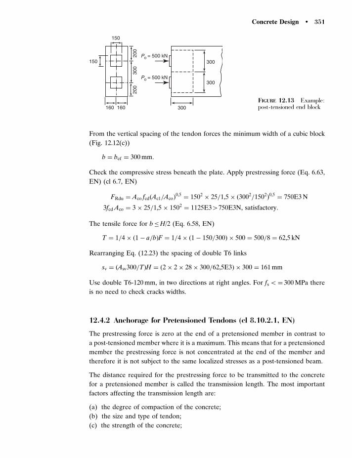
From the vertical spacing of the tendon forces the minimum width of a cubic block
(Fig. 12.12(c))
b ¼ bef ¼ 300 mm:
Check the compressive stress beneath the plate. Apply prestressing force (Eq. 6.63,
EN) (cl 6.7, EN)
FRdu ¼ Aco fcdðAc1=AcoÞ0,5
¼ 1502 � 25=1,5 � ð3002=1502Þ0,5
¼ 750E3 N
3fcd Aco ¼ 3 � 25=1,5 � 1502 ¼ 1125E34750E3N, satisfactory:
The tensile force for b�H/2 (Eq. 6.58, EN)
T ¼ 1=4 � ð1 � a=bÞF ¼ 1=4 � ð1 � 150=300Þ � 500 ¼ 500=8 ¼ 62,5 kN
Rearranging Eq. (12.23) the spacing of double T6 links
sv ¼ ðAsv300=TÞH ¼ ð2 � 2 � 28 � 300=62,5E3Þ � 300 ¼ 161 mm
Use double T6-120 mm, in two directions at right angles. For fs5¼ 300 MPa there
is no need to check cracks widths.
12.4.2 Anchorage for Pretensioned Tendons (cl 8.10.2.1, EN)
The prestressing force is zero at the end of a pretensioned member in contrast to
a post-tensioned member where it is a maximum. This means that for a pretensioned
member the prestressing force is not concentrated at the end of the member and
therefore it is not subject to the same localized stresses as a post-tensioned beam.
The distance required for the prestressing force to be transmitted to the concrete
for a pretensioned member is called the transmission length. The most important
factors affecting the transmission length are:
(a) the degree of compaction of the concrete;
(b) the size and type of tendon;
(c) the strength of the concrete;
300
Po = 500 kN
Po = 500 kN
160160
150
150
200
300
200
300
300
FIGURE 12.13 Example:post-tensioned end block
Concrete Design � 351

(d) the deformation and surface condition of the steel;
(e) sudden release of the tendon when the force is transferred to the concrete which
in practice is to be avoided.
At release the prestress may be assumed to be transferred to the concrete by a
constant bond stress (Eq. 8.15, EN)
fbpt ¼ �p1�1 fctdðtÞ
It is important to distinguish the following lengths.
(1) The transmission length (lpt) over which the prestressing force (Po) from a
pretensioned tendon is fully transmitted to the concrete, which is related to
the type and diameter of tendon and concrete strength (Eq. 8.16, EN)
lpt ¼ �1�2�pmo=fbpt ð12:24Þ
The design value is either 0,8lpt or 1,2lpt whichever is less favorable for the
effect considered.
(2) The dispersion length (ldisp) over which the concrete stresses gradually disperse
to a linear distribution across the concrete section. For rectangular cross
sections and straight tendons, situated near the bottom of a section, the
dispersion length (Eq. 8.19, EN)
ldisp ¼ ðl2pt þ d2Þ0,5
ð12:25Þ
(3) The anchorage length (lba) over which the ultimate tendon force (Fpu) in
pretensioned members is fully transmitted to the concrete.
The start of the effective bond should take account of tendons purposely debonded
at the ends and a neutralized zone in the case of sudden release. The existence
of a transmission length in a pretensioned member means that the full prestressing
force is not developed until the end of the transmission length, and consequently,
over the transmission length, the bending and shear resistances are reduced.
Example 12.8 Anchorage for pretensioned tendons.
Design the pretensioned prestressed concrete beam shown in Fig. 12.14. The beam is
simply supported over a span of 8 m and carries a uniformly distributed design load
of 375 kN at the ultimate limit state. The beam has been designed to meet the
requirements for bending. At transfer the concrete Grade is C25/30.
The critical section is at the end of the dispersion length.
Basic transmission length (Eq. 8.16, EN)
lpt ¼ �1�2�pmo=fbpt ¼ 1,0 � 0,25 � 5 � 1085=1,2 ¼ 1130 mm
352 � Chapter 12 / Prestressed Concrete

where (Eq. 8.15, EN)
fbpt ¼ �p1�2 fcdtðtÞ ¼ 2,7 � 1,0 � 0,7 � 2,57=1,5 ¼ 1,2 MPa:
Design transmission length (Eq. 8.18, EN)
lpt ¼ 1,2 � 1130 ¼ 1356 mm:
Dispersion length (Eq. 8.19, EN)
ldisp ¼ ðl2pt þ d2Þ0,5
¼ ð13562 þ 4452Þ0,5
¼ 1427 mm:
Maximum shear force at the supports Vmax¼W/2¼ 375/2¼ 187,5 kN
Reduced design shear stress at d¼ 445 mm from end of beam where bw¼ 80 mm
thickness (cl 6.2.1(8), EN)
vEd ¼ ðL=2 � dÞ=ðL=2ÞVmaxlðbwdÞ
¼ ð8E3=2 � 445Þ=ð8E3=2Þ � 187,5E3=ð80 � 445Þ ¼ 4,68 MPa
Area of cross section
Ac ¼ 600 � 300 � 220 � 325 ¼ 108,5E3 mm2
udl = 375 kN at ultimate load
8m
375 300
155
40−5 mm f wiresfck = 40
15 MPa(after losses)
600
250
7510
075
100
80
300
8m span
(b) Beam at support (c) Cross section (d) Prestress
187,5 kN
(a) Shear force diagram
−
+
°
scp
FIGURE 12.14 Example: end block for a pretensioned member
Concrete Design � 353

From the build-up of prestress (Fig. 12.14) at the neutral axis 445 mm from the end
of the beam
cp ¼ ð15=2Þd=lpt ¼ 7,5 � 445=1356 ¼ 2,46 MPa
Shear stress resistance without shear reinforcement (Eq. 6.2a, EN)
vRd,c ¼ CRd,ckð100 l fckÞ1=3
þ 0,15cp
¼ 0,18=1,5 � 1,204ð100 � 0,02 � 40Þ1=3 þ 0,15 � 2,46
¼ 0,9915VEdð4,68ÞMPa, therefore shear reinforcement required:
Depth factor
k ¼ 1 þ ð200=dÞ0,5¼ 1 þ ð200=ð600 � 155ÞÞ0,5
¼ 1,20452
Longitudinal steel ratio (cl 6.2.2(1), EN)
l ¼ 785=ð80 � 445Þ ¼ 0,02240,02: Usel ¼ 0,02:
Minimum area of longitudinal steel (cl 9.2.1.1, EN)
l,min ¼ 0,26fctm=fyk ¼ 0,26 � 3,5=1770 ¼ 0,0005145lð0,02Þ, acceptable:
Minimum shear resistance Eq. (6.2b, EN)
ðvmin þ k1cpÞ ¼ 0,035k1,5f 0,5ck þ 0,15cp
¼ 0,035 � 1,2041,5 � 400,5 þ 0,15 � 2,46
¼ 0,6615vRd,cð0,991ÞMPa, acceptable:
Shear reinforcement to resist all of the shear force using T10 single vertical stirrups
Asw=sl ¼ ðvEdbwdÞ=ð0,9d fywdÞ ¼ 4,68 � 80=ð0,9 � 0,8 � 500Þ ¼ 1,04
sl ¼ 2 � 79=1,04 ¼ 151,9 mm: Use sl ¼ 140 mm:
Maximum shear resistance (Eq. 6.9, EN)
vRd,max ¼ �cwbw0,9d v1fcd=½ðcot � þ tan �Þbwd�
¼ 1,09 � 0,9 � 0,6 � ð40=1,5Þ=2 ¼ 7,854vEdð4,68ÞMPa, acceptable:
where
04cpð2,46Þ50,25fcdð6,67ÞMPa
�cw ¼ 1 þ cp=fcd ¼ 1 þ 2,46=ð40=1,5Þ ¼ 1,09
354 � Chapter 12 / Prestressed Concrete

Shear reinforcement ratio of single T10 vertical stirrups (Eq. 9.4, EN)
w ¼ Asw=ðs1bw sin �Þ ¼ 2 � 79=ð140 � 80 � 1Þ ¼ 0,0141
Minimum shear reinforcement (Eq. 9.5, EN)
w, min ¼ 0,08f 0,5ck =fyk ¼ 0,08 � 400,5=500 ¼ 0,0015wð0,0141Þ, acceptable:
Maximum longitudinal spacing of stirrups (Eq. 9.6, EN)
sl,max ¼ 0,75dð1 þ cot �Þ ¼ 0,75 � 445 � 1 ¼ 3344slð140Þmm, acceptable:
Check shear stress failure in web (cl 12.6.3, EN)
�cp � fcvd
Check which equation from the European Code is applicable
cp ¼ 2,46 MPa
c,lim ¼ fcd � 2½ fctdð fctd þ fcdÞ�0,5
¼ 40=1,5 � 2½ð3,5=1,5Þð3,5=1,5 þ 40=1,5Þ�0,5¼ 10,2 MPa
cp(2,46)5c,lim(10,2) MPa, therefore use principal tensile stress criterion
(Eq. 12.5, EN).
Concrete design stress in shear and compression
fcvd ¼ ð f 2ctd þ cpfctdÞ
0,5¼ ðð3,5=1,5Þ2 þ 2,46 � ð3,5=1,5ÞÞ0,5
¼ 3,35 MPa
Shear stress in web of beam (Eq. 12.4, EN)
�cp ¼ 1,5ðL=2 � dÞ=ðL=2ÞVmax=Ac
¼ 1,5ð8E3=2 � 445Þ=ð8E3=2Þ � 187,5E3=108,5E3
¼ 2,305fcvdð3,35ÞMPa, acceptable:
Compression reinforcement (Eq. 6.18, EN)
Asl ¼ 0,5vEdbwdðcot � � cot�Þ=fyd
¼ 0,5 � 4,68 � 80 � 445=ð500=1,15Þ ¼ 191,6 mm2: Use 2T12 ¼ 226 mm2:
12.4.3 Uneven Distribution of Prestress
Cracks sometimes occur in the ends of pretensioned members, which are not
rectangular in cross section, as shown in Fig. 12.15. This defect is likely to occur
Concrete Design � 355
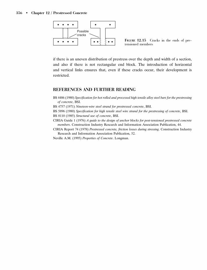
if there is an uneven distribution of prestress over the depth and width of a section,
and also if there is not rectangular end block. The introduction of horizontal
and vertical links ensures that, even if these cracks occur, their development is
restricted.
REFERENCES AND FURTHER READING
BS 4486 (1980) Specification for hot rolled and processed high tensile alloy steel bars for the prestressing
of concrete, BSI.
BS 4757 (1971) Nineteen-wire steel strand for prestressed concrete, BSI.
BS 5896 (1980) Specification for high tensile steel wire strand for the prestressing of concrete, BSI.
BS 8110 (1985) Structural use of concrete, BSI.
CIRIA Guide 1 (1976) A guide to the design of anchor blocks for post-tensioned prestressed concrete
members. Construction Industry Research and Information Association Publication, 44.
CIRIA Report 74 (1978) Prestressed concrete, friction losses during stressing. Construction Industry
Research and Information Association Publication, 52.
Neville A.M. (1995) Properties of Concrete. Longman.
Possiblecracks
FIGURE 12.15 Cracks in the ends of pre-tensioned members
356 � Chapter 12 / Prestressed Concrete
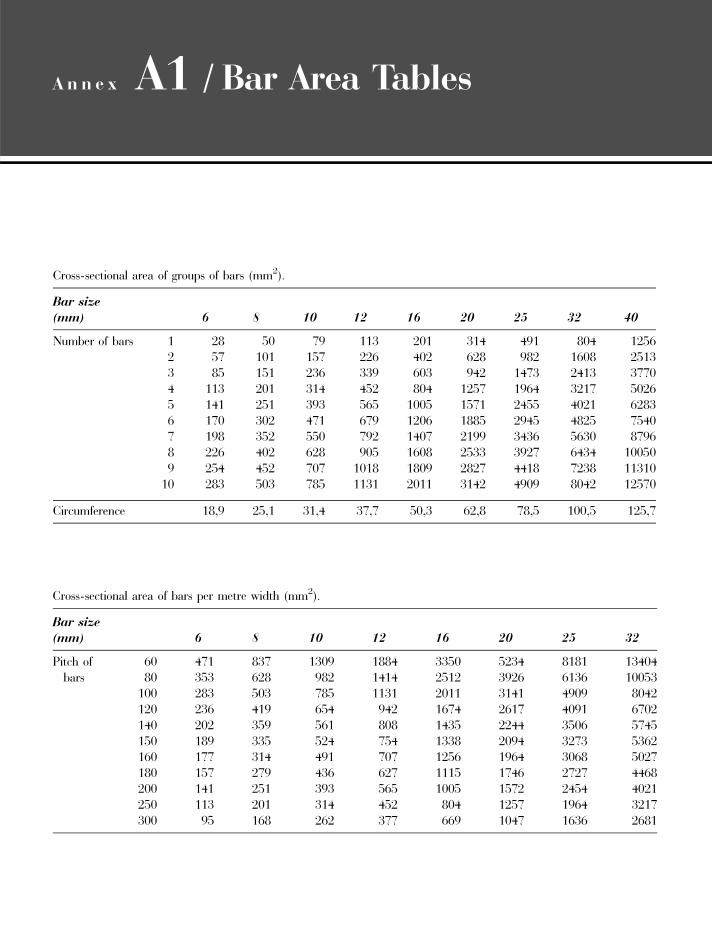
A n n e x A1 / Bar Area Tables
Cross-sectional area of bars per metre width (mm2).
Bar size(mm) 6 8 10 12 16 20 25 32
Pitch ofbars
60 471 837 1309 1884 3350 5234 8181 1340480 353 628 982 1414 2512 3926 6136 10053100 283 503 785 1131 2011 3141 4909 8042120 236 419 654 942 1674 2617 4091 6702140 202 359 561 808 1435 2244 3506 5745150 189 335 524 754 1338 2094 3273 5362160 177 314 491 707 1256 1964 3068 5027180 157 279 436 627 1115 1746 2727 4468200 141 251 393 565 1005 1572 2454 4021250 113 201 314 452 804 1257 1964 3217300 95 168 262 377 669 1047 1636 2681
Cross-sectional area of groups of bars (mm2).
Bar size(mm) 6 8 10 12 16 20 25 32 40
Number of bars 1 28 50 79 113 201 314 491 804 12562 57 101 157 226 402 628 982 1608 25133 85 151 236 339 603 942 1473 2413 37704 113 201 314 452 804 1257 1964 3217 50265 141 251 393 565 1005 1571 2455 4021 62836 170 302 471 679 1206 1885 2945 4825 75407 198 352 550 792 1407 2199 3436 5630 87968 226 402 628 905 1608 2533 3927 6434 100509 254 452 707 1018 1809 2827 4418 7238 1131010 283 503 785 1131 2011 3142 4909 8042 12570
Circumference 18,9 25,1 31,4 37,7 50,3 62,8 78,5 100,5 125,7

A n n e x A2 / Extract fromEN 1992-1-1:2003(E)
Strength and deformation characteristics for concrete.
Strength classes for concreteAnalytical relation/Explanation
fck (MPa) 12 16 20 25 30 35 40 45 50 55 60 70 80 90
fck,cube (MPa) 15 20 25 30 37 45 50 55 60 67 75 85 95 105
fcm (MPa) 20 24 28 33 38 43 48 53 58 63 68 78 88 98 fcm¼ fckþ 8 (MPa)
fctm (MPa) 1,6 1,9 2,2 2,6 2,9 3,2 3,5 3,8 4,1 4,2 4,4 4,6 4,8 5,0 fctm¼ 0,30� fck(2/3)
�C50/60
fctm¼ 2,12
ln(1þ ( fcm /10))4C50/60
fctk,0,05(MPa)
1,1 1,3 1,5 1,8 2,0 2,2 2,5 2,7 2,9 3,0 3,1 3,2 3,4 3,5 fctk;0,05¼ 0,7� fctm5% fractile
fclk,0.95(MPa)
2,0 2,5 2,9 3,3 3,8 4,2 4,6 4,9 5,3 5,5 5,7 6,0 6,3 6,6 fclk;0,95¼ 1,3� fctm95% fractile
Ecm (GPa) 27 29 30 31 33 34 35 36 37 38 39 41 42 44 Ecm¼ 22[( fcm)/10]0,3
( fcm inMPa)
"c1 (ø) 1,8 1,9 2,0 2,1 2,2 2,25 2,3 2,4 2,45 2,5 2,6 2,7 2,8 2,8 see Figure 3.2
"c1(ø)¼ 0,7 f 0;31cm 5 2,8
"cu1 (ø) 3,5 3,2 3,0 2,8 2,8 2,8 see Figure 3.2 for fck� 50MPa
"cu1(ø)¼ 2,8þ 27
[(98� fcm)/100]4
"c2 (ø) 2,0 2.2 2,3 2,4 2,5 2,6 see Figure 3.3 for fck� 50MPa
"c2(ø)¼ 2,0þ 0,085
( fck� 50)0,53
"cu2 (ø) 3,5 3,1 2,9 2,7 2,6 2,6 see Figure 3.3 for fck� 50MPa
"cu2(ø)¼ 2,6þ 35
[(90� fck)/100]4
n 2,0 1,75 1,6 1,45 1,4 1,4 for fck� 50MPa
n¼ 1,4þ 23,4
[(90� fck)/100]4
"c3 (ø) 1,75 1,8 1,9 2,0 2,2 2,3 see Figure 3.4 for fck� 50MPa
"c3(ø)¼ 1,75þ 0,55
[( fck� 50)/40]
"cu3 (ø) 3,5 3,1 2,9 2,7 2,6 2,6 see Figure 3.4 for fck� 50MPa
"cu3(ø)¼ 2,6þ 35
[(90� fck)/100]4

A n n e x B1 / Design Graph for DoublyReinforced Beams
0,3
0,2
0,1
00,010,1
0,020,2
0,030,3
0,040,4 0,5
0,20
0,10
0,05
0,00
M/bd 2fck
A′ s
f yk/
bdf c
kAsfyk/bdfck
p = As/bd
fck = 50
fyk = 500
d/h = 0,85
Design graph for doubly reinforced beams
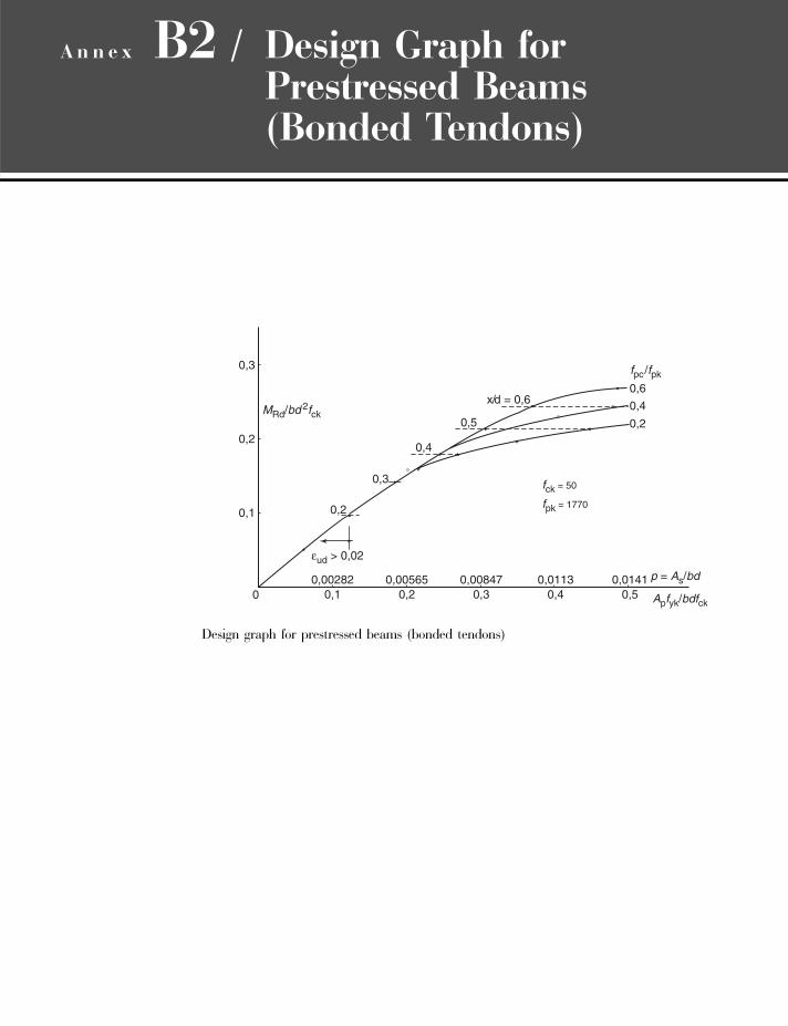
A n n e x B2 / Design Graph forPrestressed Beams(Bonded Tendons)
0,3
0,2
0,1
00,00282
0,10,00565
0,20,00847
0,30,0113
0,40,0141
0,5
MRd/bd 2fck
fpc/fpk
fpk = 1770
fck = 50
Apfyk/bdfck
p = As/bd
0,6
0,4
0,2
0,2
0,3
0,4
0,5
x/d = 0,6
εud > 0,02
Design graph for prestressed beams (bonded tendons)

A n n e x B3 / Design Graph for aRectangular Column
0 0,1 0,2 0,3 0,4 0,5
0,5
1,0
1,5
2,0
α = 0 α = 0,2 α = 0,4 α = 0,6 α = 0,8 α = 1,0 α = 1,2 α = 1,4
N/bhfck
M/bh2fck
d/h = 0,85
b
dh
As2
As2
fyk = 500
fck = 50α = Asfyk/bdfck
Design graph for a rectangular column
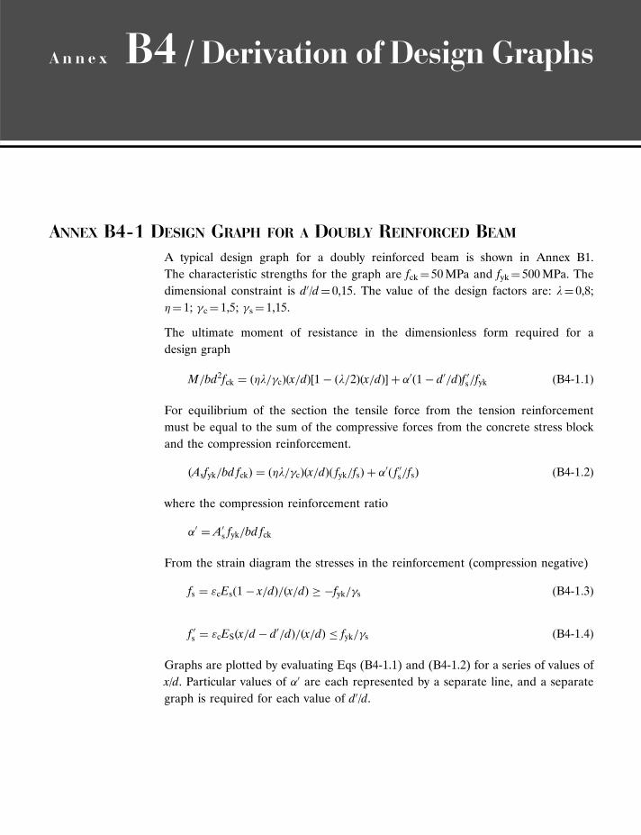
A n n e x B4 / Derivation of Design Graphs
ANNEX B4-1 DESIGN GRAPH FOR A DOUBLY REINFORCED BEAM
A typical design graph for a doubly reinforced beam is shown in Annex B1.
The characteristic strengths for the graph are fck¼ 50 MPa and fyk¼ 500 MPa. The
dimensional constraint is d0/d¼ 0,15. The value of the design factors are: l¼ 0,8;
�¼ 1; �c¼ 1,5; �s ¼ 1,15.
The ultimate moment of resistance in the dimensionless form required for a
design graph
M=bd2fck ¼ ð�l=�cÞðx=dÞ½1 � ðl=2Þðx=dÞ� þ �0ð1 � d0=dÞf 0s=fyk ðB4-1:1Þ
For equilibrium of the section the tensile force from the tension reinforcement
must be equal to the sum of the compressive forces from the concrete stress block
and the compression reinforcement.
ðAsfyk=bd fckÞ ¼ ð�l=�cÞðx=dÞð fyk=fsÞ þ �0ð f 0s=fsÞ ðB4-1:2Þ
where the compression reinforcement ratio
�0 ¼ A0s fyk=bd fck
From the strain diagram the stresses in the reinforcement (compression negative)
fs ¼ "cEsð1 � x=dÞ=ðx=dÞ � �fyk=�s ðB4-1:3Þ
f 0s ¼ "cESðx=d� d0=dÞ=ðx=dÞ � fyk=�s ðB4-1:4Þ
Graphs are plotted by evaluating Eqs (B4-1.1) and (B4-1.2) for a series of values of
x/d. Particular values of �0 are each represented by a separate line, and a separate
graph is required for each value of d0/d.

ANNEX B4-2 DESIGN GRAPH FOR A PRESTRESSED BEAM
The equations for a doubly reinforced beam can be modified for prestressed
concrete beams with �0 ¼ 0. The steel stress is increased by the prestress and limited
to fpk/�c¼ 1770/1,15 MPa. The steel strain is also increased by the prestress and
limited to 0,02.
ANNEX B4-3 DESIGN GRAPH FOR A RECTANGULAR COLUMN
A typical design graph for a column is shown in Annex B3. The characteristic
strength for the column graph are fck¼ 50 MPa and fyk¼ 500 MPa. The dimensional
constraint is d/h¼ 0,85 and the values of the design factors are: l¼ 0,8; �¼ 1;
�c¼ 1,5; �s¼ 1,15.
From equilibrium of axial forces on a column in dimensionless form
N=bh fck ¼ ð�l=�cÞðx=hÞ þ n� ðB4-3:1Þ
From equilibrium of bending moments acting about an axis at mid-height of the
section
M=bh2fck ¼ ð�l=�cÞðx=hÞ½0,5 � ðl=2Þ x=h� þm� ðB4-3:2Þ
where
n ¼ ð f1 þ f2Þ=ð2fykÞ
m ¼ ð2d=h� 1Þð f1 � f2Þ=ð4fykÞ
� ¼ Asc fyk=bhfck
Stresses in the steel
f1 ¼ "cEsðx=h� 1 þ d=hÞ=ðx=hÞ � �fyk=�s ðB4-3:3Þ
f2 ¼ "cEsðx=h� d=hÞ=ðx=hÞ � �fyk=�s ðB4-3:4Þ
The case when l x� h, i.e. when the concrete stress block covers the whole section,
must also be considered. In this case f1 is equal to the design strength in compression
and there is no moment from the stress block and hence Eqs (B4-3.1) and (B4-3.2)
become
N=bhfck ¼ �=�c þ n� ðB4-3:5Þ
M=bh2fck ¼ m� ðB4-3:6Þ
where
n ¼ ð1 þ �2 f2=fykÞ=ð2�sÞ
m ¼ ð2d=h� 1Þð1 � �s f2=fykÞ=ð4�sÞ
Concrete Design � 363

A n n e x C / Subframes
This annex details analysis results from simple subframes which may used for pre-
liminary analyses of frame structures. They are now less used for the final analysis
owing to the widespread availability of commercial software. Also it should be
noted that they take no account of the co-existent horizontal forces that must be
applied as part of the load cases involving vertical loads.
The results given here have been obtained using slope-deflection with the follow-
ing sign convention: clockwise positive for moments and rotations. Settlement of
supports has not been considered.
For both ends fixed, the moments at either end MAB and MBA are given by
MAB ¼2EI
LAB2�A þ �Bð Þ þM12 ðC1Þ
and
MBA ¼2EI
LAB2�B þ �Að Þ þM21 ðC2Þ
where EI/L is the stiffness of the member, �A and �B are the rotations at either
end and M12 and M21 are the fixed end moments at ends A and B, respectively due
to the loading applied to the member. The fixed end moments for a partial UDL,
a point load and equal end triangular loading are given in Fig. C1.
If one end is pinned (for example, end B, then MBA¼ 0), then MAB becomes,
MAB ¼3EI
LAB�A þM12 �
M12
2ðC3Þ
A similar expression can be derived for end A pinned.
For convenience, the stiffness EI/L has been denoted as k (the full value of k has
been used in all the derivations).
Subframe 1: Single beam and column (Fig. C2):
a) End F fixed
MAB ¼ �MAF ¼ �kCL
kB1 þ kCLM11 ðC4Þ
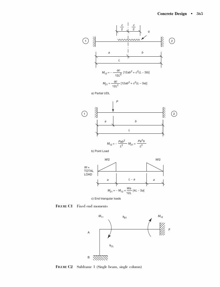
a
M12 = −
M21 =
M12 = −Pab2
Wa
12L[4L − 3a]
Pa2b
L2
W/2W/2
L − aa
W =TOTALLOAD
a
L2M21 =
M21 = − M12 =
a) Partial UDL
b) Point Load
c) End triangular loads
q
c2
b
L
P
a b
L
qc
qc
12L2
12L2
[12ab2 + c2(L − 3b)]
[12ab2 + c2(L − 3a)]
1 2
1 2
c2
FIGURE C1 Fixed end moments
AF
M11 M12kB1
kCL
B
FIGURE C2 Subframe 1 (Single beam, single column)
Concrete Design � 365

MFA ¼2kCLM12 þ kB1ð2M12 �M11Þ
2ðkB1 þ kCLÞðC5Þ
MBA ¼MAB
2ðC6Þ
b) End F pinned:
MAB ¼ �MAF ¼ �4kCL
3kB1 þ 4kCLM11 �
M12
2
� �ðC7Þ
MBA ¼MAB
2ðC8Þ
Subframe 2: Two beams and single column (Fig. C3):
a) Ends A and L of beam fixed:
MFA ¼ M12 �kb1
kB1 þ kB2 þ kCLðM12 þM21Þ ðC9Þ
MAF ¼ M11 �kB1
2ðkB1 þ kB2 þ kCLÞðM12 þM21Þ ðC10Þ
MFL ¼ M21 �kB2
kB1 þ kB2 þ kCLðM12 þM21Þ ðC11Þ
MLF ¼ M22 �kB2
2ðkB1 þ kB2 þ kCLÞðM12 þM21Þ ðC12Þ
MFG ¼ 2MGF ¼ �kCL
kB1 þ kB2 þ kCLðM12 þM21Þ ðC13Þ
b) Ends A and L pinned:
MFL ¼ð3kB1 þ 4kCLÞ½M21 � ðM22=2Þ� � 3kB2½M12 � ðM11=2Þ�
3kB1 þ 3kB2 þ 4kCLðC14Þ
MFA ¼ð3kB2 þ 4kCLÞ½M12 � ðM11=2Þ� � 3kB1½M21 � ðM22=2Þ�
3kB1 þ 3kB2 þ 4kCLðC15Þ
A
M11M12 M21 M22
F
kB1 kB2
kCL
L
FIGURE C3 Subframe 2 (Two beams,single column)
366 � Annex C / Subframes

MFG ¼ 2MGF ¼4 kCL
3kb1 þ 3kB2 þ 4kCL
M22 þM11
2�M21 �M12
� �ðC16Þ
Subframe 3: Column above aand below beam either side (Fig. C4):
a) Ends C and N fixed:
MHC ¼ �kB1
kB1 þ kB2 þ kCL þ kCUðM12 þM21Þ þM12 ðC17Þ
MCH ¼ �kB1
2ðkB1 þ kB2 þ kCL þ kCUÞðM12 þM21Þ þM11 ðC18Þ
MHN ¼ �kB2
kB1 þ kB2 þ kCL þ kCUðM12 þM21Þ þM21 ðC19Þ
MNH ¼ �kB2
2ðkB1 þ kB2 þ kCL þ kCUÞðM12 þM21Þ þM12 ðC20Þ
MHG ¼ 2MGH ¼ �kCU
kB1 þ kB2 þ kCL þ kCUðM12 þM21Þ ðC21Þ
MHJ ¼ 2MJH ¼ �kCL
kB1 þ kB2 þ kCL þ kCUðM12 þM21Þ ðC22Þ
b) Ends C and N pinned:
MHN ¼ð3kB1 þ 4kCL þ 4kCUÞ½M21 � ðM22=2Þ� � 3kB2½M12 � ðM11=2Þ�
3kB1 þ 3kB2 þ 4kCL þ 4kCUðC23Þ
MHC ¼ð3kB2 þ 4kCL þ 4kCUÞ½M12 � ðM11=2Þ� � 3kB1½M21 � ðM22=2Þ�
3kB1 þ 3kB2 þ 4kCL þ 4kCUðC24Þ
C NH
J
G
M11M12 M21
kCL
kB2kB1
kCUM22
FIGURE C4 Subframe 3 (Twobeams, two columns)
Concrete Design � 367

MHG ¼ 2MGH ¼4kCU
3kB1 þ3kB2 þ4kCU þ4kCL
M22 þM11
2�M21 �M12
� �ðC25Þ
MHJ ¼ 2MJH ¼4kCL
3kB1 þ 3kB2 þ 4kCU þ 4kCL
M22 þM11
2�M21 �M12
� �ðC26Þ
Subframe 4: Single beam column above and below (Fig. C5):
a) End H fixed:
MCH ¼kCL þ kCU
kB1 þ kCL þ kCUM11 ðC27Þ
MCH ¼ M12 �kB1
2ðkB1 þ kCL þ kCUÞM11 ðC28Þ
MCD ¼ 2MDC ¼ �kCL
kB1 þ kCL þ kCUM11 ðC29Þ
MCB ¼ 2MBC ¼ �kCU
kB1 þ kCL þ kCUM11 ðC30Þ
b) End H pinned:
MCH ¼4kCL þ 4kCU
3kB1 þ 4kCL þ 4kCUM11 �
M12
2
� �ðC31Þ
MCD ¼ 2MDC ¼ �4kCL
3kB1 þ 4kCL þ 4kCUM11 �
M12
2
� �ðC32Þ
MCB ¼ 2MBC ¼ �4kCU
3kB1 þ 4kCL þ 4kCUM11 �
M12
2
� �ðC33Þ
B
kCU
kCL
kB1
M11M12
C H
D
FIGURE C5 Subframe 4 (single beam, twocolumns)
368 � Annex C / Subframes
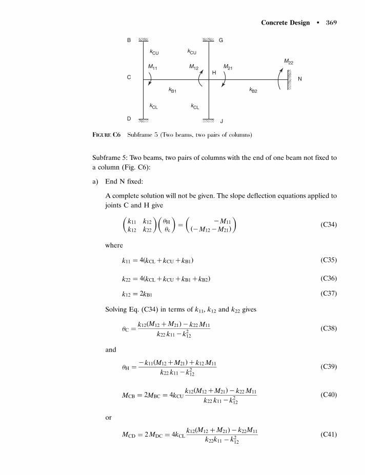
Subframe 5: Two beams, two pairs of columns with the end of one beam not fixed to
a column (Fig. C6):
a) End N fixed:
A complete solution will not be given. The slope deflection equations applied to
joints C and H give
k11 k12
k12 k22
� ��H
�c
� �¼
�M11
ð�M12 �M21Þ
� �ðC34Þ
where
k11 ¼ 4ðkCL þ kCU þ kB1Þ ðC35Þ
k22 ¼ 4ðkCL þ kCU þ kB1 þ kB2Þ ðC36Þ
k12 ¼ 2kB1 ðC37Þ
Solving Eq. (C34) in terms of k11, k12 and k22 gives
�C ¼k12ðM12 þM21Þ � k22 M11
k22 k11 � k212
ðC38Þ
and
�H ¼� k11ðM12 þM21Þ þ k12 M11
k22 k11 � k212
ðC39Þ
MCB ¼ 2MBC ¼ 4kCUk12ðM12 þM21Þ � k22 M11
k22 k11 � k212
ðC40Þ
or
MCD ¼ 2MDC ¼ 4kCLk12ðM12 þM21Þ � k22M11
k22k11 � k212
ðC41Þ
D
C
B
M11 M12 M21
M22
kCL
kB1 kB2
kCU
kCL
kCU
G
H
J
N
FIGURE C6 Subframe 5 (Two beams, two pairs of columns)
Concrete Design � 369

MHG ¼ 2MGH ¼ 4kCU� k11ðM12 þM21Þ þ k12M11
k22k11 � k212
ðC42Þ
MHJ ¼ 2MJH ¼ 4kCL� k11ðM12 þM21Þ þ k12M11
k22k11 � k212
ðC43Þ
MHN ¼ M21 þ 4kB2� k11ðM12 þM21Þ þ k12M11
k22k11 � k212
ðC44Þ
MNH ¼ M22 þ 2kB2� k11ðM12 þM21Þ þ k12M11
k22k11 � k212
ðC45Þ
MCH ¼ M11 þ 2kB1M11ðk12 �2k22Þ þ ðM12 þM21Þð2k12 � k11Þ
k22k11 � k212
ðC46Þ
MHC ¼ M12 þ 2kB1M11ð2k12 �k22Þ þ ðM12 þM21Þðk12 � 2k11Þ
k22k11 � k212
ðC47Þ
b) End N pinned:
k11 k12
k12 K22
� ��C
�H
� �¼
�M11
ð�M12 �M21 þ ðM22=2ÞÞ
� �ðC48Þ
where
k11 ¼ 4ðkCL þ kCU þ kB1Þ ðC49Þ
k22 ¼ 4kCL þ 4kCU þ 4kB1 þ 3kB2 ðC50Þ
k12 ¼ 2kB1 ðC51Þ
Solving Eq. (C48) gives
�C ¼k12ðM12 þM21 � ðM22=2ÞÞ � k22M11
k22k11 � k212
ðC52Þ
and
�H ¼�k11ðM12 þM21 � ðM22=2ÞÞ þ k12M11
k22k11 � k212
ðC53Þ
or
MCB ¼ 2MBC ¼ 4kCUk12ðM12 þM21 � ðM22=2ÞÞ � k22M11
k22k11 � k212
ðC54Þ
370 � Annex C / Subframes
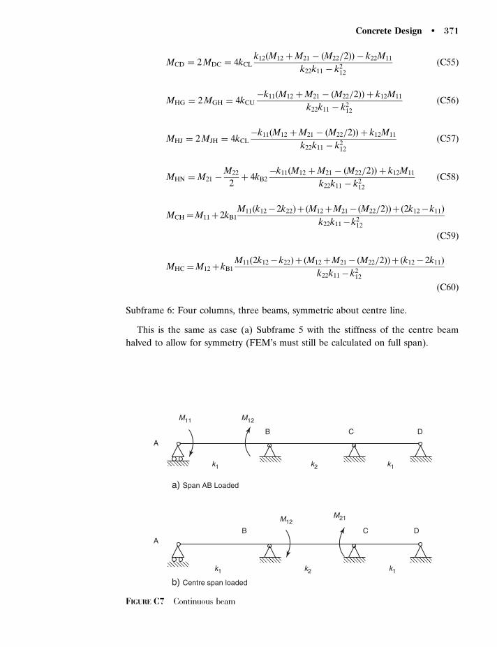
MCD ¼ 2MDC ¼ 4kCLk12ðM12 þM21 � ðM22=2ÞÞ � k22M11
k22k11 � k212
ðC55Þ
MHG ¼ 2MGH ¼ 4kCU�k11ðM12 þM21 � ðM22=2ÞÞ þ k12M11
k22k11 � k212
ðC56Þ
MHJ ¼ 2MJH ¼ 4kCL�k11ðM12 þM21 � ðM22=2ÞÞ þ k12M11
k22k11 � k212
ðC57Þ
MHN ¼ M21 �M22
2þ 4kB2
�k11ðM12 þM21 � ðM22=2ÞÞ þ k12M11
k22k11 � k212
ðC58Þ
MCH ¼M11 þ2kB1M11ðk12 �2k22Þþ ðM12 þM21 �ðM22=2ÞÞþ ð2k12 �k11Þ
k22k11 �k212
ðC59Þ
MHC ¼M12 þ kB1M11ð2k12 � k22Þþ ðM12 þM21 �ðM22=2ÞÞþ ðk12 � 2k11Þ
k22k11 � k212
ðC60Þ
Subframe 6: Four columns, three beams, symmetric about centre line.
This is the same as case (a) Subframe 5 with the stiffness of the centre beam
halved to allow for symmetry (FEM’s must still be calculated on full span).
A
B
B C D
C D
M11
M12
k1
k1
k2
k2
k1
k1
M12
M21
a) Span AB Loaded
b) Centre span loaded
A
FIGURE C7 Continuous beam
Concrete Design � 371

Subframe 7: Continuous beam.
The only case which will be considered here is a three span continuous beam with
the end spans having stiffness k1 and the centre span having stiffness k2.
Case 1: Span AB loaded (Fig. C7 (a)):
MCB ¼ �MCD ¼6k1k2
ð4k2 þ 3k1Þ2� 4k2
2
½ðM11=2Þ �M12� ðC61Þ
MBC ¼ �MBA ¼12k2ðk1 þ k2Þ
ð4k2 þ 3k1Þ2� 4k2
2
½ðM11=2Þ �M12� ðC62Þ
Case 2: Centre span loaded (Fig. C7 (b)):
MBA ¼ MCB ¼ �MBC ¼ �MCD ¼3k1
ð4k2 þ 3k1Þ2� 4k2
2
½2M22k2 �M21ð4k2 þ 3k1Þ�
ðC63Þ
372 � Annex C / Subframes

Index
Actions 1, 2, 32–40, 49, 55, 56, 70, 90,172, 206, 211, 213, 215, 250, 254,269, 272–276, 278, 288, 293,295–298, 306
accidental loading 21alkali-aggregate reaction 65, 69anchorage
bars 176curtailment 181prestressed members 348
analysisserviceability limit state 42, 217, 249,
288, 327, 330ultimate limit state 39, 216, 322, 324
area of bars 187, 357
Balanced section 107bar
area 357bending schedules 15mark 12, 14, 15splices 179, 180
beamscontinuous 50, 51, 53, 58, 59, 63, 72,
77, 97, 109, 121, 371crack widths 91, 93, 136deflection 24, 77, 338derivation of design graphs 362design graph 359, 360, 362, 363flanged 54, 119, 120, 123prestressed 2, 29, 164, 165, 323–325,
327, 338, 360, 363shear strength 29slenderness limit 47torsion 45, 266ultimate moment of resistance 324,
362bearing stresses at supports 184bending
moment envelope 37, 60resistance for prestressed concrete
321, 323, 327bends in reinforcement 15, 26, 188bent-up bars 105, 134, 140, 145–148,
151, 152biaxial bending 198, 201, 202, 204, 206,
209, 275, 280bond length 140, 157, 160, 163,
164, 176, 178, 179, 182, 183,191–196
bracing 10, 46–50, 102, 202buckling of columns 203
Carbonation 66, 67, 69characteristic action (load) 32, 33, 59characteristic strength 18–20, 72–74,
116–118, 129, 199, 333, 340, 341,362, 363
chloride attack 66, 69columns
axially load and bending moment 200biaxial bending 198, 201, 202, 204,
206, 209design graph 361, 363design method 205, 206, 210effective length 205load reduction factors 55reinforcement 161, 198second order moments 204, 211short 199, 202slender 46, 203, 204supporting flat slabs 72
concretecover 16, 66, 179, 180, 185design strength 21failure criteria 28high strength 97, 98, 101, 127manufacture 3strength tables 358
connectionsbeam-to-beam 186, 187beam-to-column 188–190, 194column-to-base 191corbel 192, 193half joint 193, 194simple beam 247
contraflexure, points of 35, 37, 59, 121corrosion of reinforcement 65, 66counterfort retaining wall 287, 307, 308cover to reinforcement 16crack
control 140width 2, 40, 70, 87, 88, 90, 91, 93, 102, 136,
148, 249, 293, 300–302parallel to reinforcement 68, 69
cracking, early thermal 70, 88, 89,293, 302
creep of concrete 343, 348curtailment of bars 176, 182, 183
Deflectionreinforced beams 72, 73
designenvelope 35, 36graphs 201, 205, 208, 362

design (continued)limit state 9, 10, 39statistical basis 7strength 9, 20, 21
detailing 12, 14, 56, 65, 68, 90, 100, 114,172, 180, 181, 242, 247, 249, 268
doubly reinforced beams 115, 117, 129,211, 362, 363
drawings 6, 11, 12, 14, 16
Early thermal cracking 88, 89, 293, 302effective
depth 39, 65, 71–74, 108, 113, 114,116–118, 124, 126, 127, 129, 132, 182, 185,193, 252, 267, 268, 280, 283, 299, 302,310, 312,323, 337
length of a column 205width of flange 54, 73, 120, 121, 123spans 132
elastic analysisdeformation of concrete 341prestressed beams 40
end blocks 349, 350envelope
bending moment 37, 53, 60shear force 53, 62
errors 10, 11, 243, 252
Failure criteria 27–29fans, yield line 238–242fatigue 11, 21, 26, 27fire
beams and slabs 97calculation methods 97columns 95high strength concrete 97tabular data 94spalling 98whole building behaviour 101
flangebeams 54, 119effective width 54, 73, 120, 121, 123, 124
flat slabs 40, 54, 73, 215, 265–267foundations 1, 37, 68, 70, 151, 152, 155,
184, 269–272, 274, 278, 279, 281, 299frame classification 48frame imperfections 46friction loss 344
Grade of concrete 155
Hillerborg strip method 40, 120, 215,217, 246–248, 254, 256, 258, 265, 308,310, 319
Isotropic orthogonal reinforcement 222
Johansen yield line method 40, 216, 218
Lateral torsional buckling 45limit state design 9, 10, 39links – see stirrups 13–15, 105, 107, 134,
135, 137–152, 154, 159, 160, 162, 163,166–168, 171–174, 179, 186, 189–196,198, 199, 265, 267, 268, 281, 314–317,350, 351, 356
loads (see actions) 32–37lower bound solution 39, 40, 56, 217, 246
Membrane action 218modulus of elasticity
concrete 23, 170, 338steel 21, 201
moment–curvature 107, 108moment of resistance
reinforced concrete beams 110, 113,114, 127
prestressed concrete beams 322, 324
Neutral axis depth 39, 56, 57, 108, 109, 111,117, 127, 216, 300, 316
non-sway frame 2, 47, 48
Optimum section 334orthogonal reinforcement 222over-reinforced section 107overturning 10, 34, 35, 43–45, 272, 287, 289,
290, 294, 308, 309
Pad foundation 155, 270, 271, 279partial safety factors 9, 43, 272, 273pile foundations 158prestressed concrete
analysis 322anchorage 348deflection 337–340derivation of design graphs 362, 363design 330design graphs 360loss of prestress 340–348
progressive collapse 10, 41punching shear 41, 43, 134, 151, 154, 155,
157, 159, 160, 215, 265, 280, 282
Redistribution 39, 40, 55, 56–63, 94, 97,109, 116–118, 124, 128–130, 132, 216,217, 254, 274
reinforcementbar area tables 357strength 73, 97, 168curtailment 181design strength 48
retaining wallbase 287–299, 303, 306, 308–310, 312,
313, 315, 318, 319counterfort 287, 307, 308gravity (mass) 287overturning 287, 289, 290, 294, 308, 309
374 � Index

partial safety factor 289, 290, 291, 303settlement 288, 305sized 308sliding 287, 288, 290–295, 297–299, 310stability 286, 287, 293, 307stem 287, 288, 293, 299, 300, 307, 308surcharge 288, 294–298, 300, 306, 309–311tilt 288, 305, 306
robust 4
St.Venant torsional factors 170serviceability limit state 10, 26, 34, 37,
42, 70, 198, 217, 249, 288, 327,330, 331, 333
crack spacing 88, 89crack width 87, 88, 90, 91, 93deflection 70–73, 77, 78, 85–87fire 71
shearbase 155, 156, 158bent-up bars 134, 140, 145–148, 151, 152corbels 160, 164failure 133, 134, 150, 153, 159, 164flange for a ‘T’ beam 148links 134, 140pad foundation 155pile caps 158prestressed beams 164, 165reinforcement 132, 134, 135, 137, 139,
142, 143, 145–147, 150–152, 154, 155,158–160, 162, 163, 166, 171, 174
‘T’ beams 148, 149resistance of flat slabs 151theory 171torsion 168–174
shrinkage of concrete 342, 348site conditions 16, 21slabs
cantilever 237circular 235, 236concentrated loads 265curtailment 249deflection 217, 249, 252, 253, 264, 267detailing 249edge beams 258, 259elastic analysis 266encastre 222, 254flat 40, 265–267Hillerborg strip method 215, 217,
246–248, 254, 256, 258, 265Johansen yield line 216, 218lower bound solution 217, 246nodal force approach 218, 219rectangular 224, 227, 228, 247, 250shear resistance 265square 222, 238, 239, 242, 244, 245, 258,
259, 265support beams 258, 260torsion 249, 267
triangular 230, 231, 233types 215, 216upper bound solution 217, 218virtual work approach 218waffle 215, 267, 268
slenderness ratio 47, 96, 205–207, 212, 213stability
columns 46manufacture of steel 5members 45structure 43
standard deviation 8, 18, 19stress–strain relationships 22strip method, Hillerborg 40, 120, 215,
217, 246–248, 254, 256, 258, 265,308, 310, 319
subframecontinuous beam 371one end 364
sulfate attack 65, 70
Taumasite attack 70testing of reinforced concrete materials 30thermal
strain 26cracking 88, 89, 293, 302
ties 42, 43tolerances 11, 12, 16, 271, 282torsion
constant 169, 170equivalent thin walled section 170, 171modes of failure 168, 169plain concrete 168–171reinforcement 171–173stiffness 169, 170
transmission length 351–353
Ultimate limit statecolumns 199reinforced beams 106prestressed beams 322
under-reinforced beam 56, 218upper bound theorem, slabs 216–218
Vibration 10, 33, 34, 70
Waffle slab 55, 267, 268wind loading 27, 45, 70
Yield line analysisconcentrated load 265isotropic orthogonal reinforcement 222Johansen 216, 218, 219lower bound solution 217, 246orthogonal reinforcement 222part fan 237, 239, 244upper bound solution 217, 218virtual work method 218
Index � 375


![How to Design Concrete Structures Using Eurocode 2[1]](https://img.dokumen.tips/doc/110x75/577cdd1a1a28ab9e78ac38c6/how-to-design-concrete-structures-using-eurocode-21.jpg)