Embed Size (px)
Citation preview


2
Concept Specifications/Prerequisites for DeepWind Deliverable D8.1 Uwe Schmidt Paulsen, Signe Schløer, Xiaoli Larsén, Andrea Hahmann, Søren Larsen, Torben Larsen, Ole Svenstrup Petersen(DHI) DTU Wind Energy E0059(EN) July 2014
PP129
Dep
artm
ent
of
Win
d E
ner
gy
E R
epo
rt 2
014
Concept Specifications/Prerequisites for DeepWind Deliverable D8.1
Uwe Schmidt Paulsen, Signe Schløer, Xiaoli Larsén, Andrea Hahmann, Søren Larsen, Torben Larsen, Ole
Svenstrup Petersen(DHI)
DTU Wind Energy E0059(EN)
July 2014

Authors: Uwe Schmidt Paulsen, Signe Schløer, Xiaoli Larsén, Andrea
Hahmann, Søren Larsen, Torben Larsen, Ole Svenstrup Petersen(DHI)
Title: Deliverable D8.1
Department: DTU WE
DTU Wind Energy E0059(EN)
July 2014
ISBN 978-87-92896-98-8
Summary (max 2000 characters):
The work is a result of the contributions within the DeepWind project which is
supported by the European Commission, Grant 256769 FP7 Energy 2010-
Future emerging technologies, and by the DeepWind beneficiaries: DTU(DK),
AAU(DK), TUDELFT(NL), TUTRENTO(I), DHI(DK), SINTEF(N), MARINTEK(N),
MARIN(NL), NREL(USA), STATOIL(N), VESTAS(DK) and NENUPHAR(F).
The report discuss the design considerations for offshore wind turbines , both in
general and specifically for Darrieus-type floating turbines, as is the focus of
the DeepWind project. The project is considered in a North Sea environment,
notably close to the Norwegian South West coast, at the site of the Hywind
demonstration project.
The report summarises standard characteristics for the North Sea and the
Baltic, formulated by earlier EU projects, and compare these to the conditions
met at the project site. Comparison s with existing measured met-ocean data
are carried out.
Similarly scaling considerations from the earlier projects are presented and
seen in relation to and contrasted to the needs of the current project.
Contract no.:
256769
Project no.:
43057
Sponsorship:
European Commission-FP7
under contract 256769
Front page:
DeepWind Baseline 5MW
conceptual design
Pages: 129
Tables: 19
Referencer: 84
Technical University of Denmark Department of Wind Energy Frederiksborgvej 399 Building 118 4000 Roskilde Denmark Telephone 21329405 [email protected] www.vindenergi.dtu.dk


Preface
The hypothesis of DeepWind is that this concept is developed specifically for offshore application and has potentials for better cost efficiency than existing offshore technology. Based on this hypothesis the objectives are:
i. to explore the technologies needed for development of a new and simple floating offshore concept with a vertical axis rotor and a floating and rotating foundation,
ii. to develop calculation and design tools for development and evaluation of very large wind turbines based on this concept and
iii. evaluation of the overall concept with floating offshore horizontal axis wind turbines. Upscaling of large rotors beyond 5MW has been expressed to have more cost potentials for vertical axis wind turbines than for horizontal axis wind turbines due to less influence of cyclic gravity loads. However, the technology behind the proposed concept presents extensive challenges needing explicit research, especially: • dynamics of the system, • pultruded blades with better material properties, • sub-sea generator, • mooring and torque absorption system, and • torque, lift and drag on the rotating and floating haft foundation.
In order to be able in detail to evaluate the technologies behind the concept the project comprises: 1. numerical tools for prediction of energy production, dynamics, loads and fatigue, 2. tools for design and production of blades 3. tools for design of generator and controls, 4. design of mooring and torque absorption systems, and 5. knowledge of friction torque and lift and drag on rotating tube.
The technologies need verification, and in the project verification is made by: 6. proof-of concept testing of a small, kW sized technology demonstrator, partly under real
conditions, partly under controlled laboratory conditions, 7. integration of all technologies in demonstration of the possibility of building a 5 MW wind
turbine based on the concept, and an evaluation of the perspectives for the concept. The results of WP01, WP02, WP03, WP04, WP05, and WP06 are integrated into a conceptual study of a new 5 MW design for comparison and evaluation against existing 5MW offshore horizontal axis wind turbine technology. Upscaling is explored against scaling trends from a 5 MW prototype towards a final 20 MW ‘exercise’. Cost elements affecting the distribution of cost are surveyed, and effects with cost advantage potential are considered and the exercise accentuates differences of the concept compared to a 5 MW/ 20 MW offshore horizontal – axis turbine technologies. The results from the technical work packages are readdressed in terms of capitalised knowledge in the new technology field embracing compliance, safety and standards for offshore wind energy converters and the cost projections for upscaling are estimated by different levels of complexity. The conditions at site are discussed and explained for the final design layout calculations in WP01, Task 1.2. Applications of code, standards and regulations as well as decommissioning are surveyed into the calculations of the 5 MW design layout. This report describes site conditions which are relevant to apply for the present design.
Risø, July 2014 Uwe Schmidt Paulsen
Project manager and Co-ordinator of DeepWind
Deliverable D8.1

- 6 - Deliverable D8.1
Contents
Summary ........................................................................................................................................ 9
1. INTRODUCTION................................................................................................................ 11
2. CHARACTERISTICS OF SHALLOW TO MEDIUM DEEP SEA OFFSHORE WIND
–WAVE CLIMATE .............................................................................................................. 11 2.1 Sources of Data ............................................................................................................................... 12 2.2 Parameters for wind and wave specification .................................................................................... 13 2.3 One –parameter climate based on wind speed. ............................................................................... 14 2.4 Standard offshore conditions for testing and modelling ................................................................... 26
3. DEEP SEA OFFSHORE MET-OCEAN CONDITIONS-THE SITE OF DEEPWIND
(SITE KARMØY) ................................................................................................................ 34 3.1 General considerations .................................................................................................................... 34 3.2 Deep Sea Ocean waves characteristics ........................................................................................... 35 3.3 Currents ........................................................................................................................................... 43 3.4 Wind assessment, wind distribution assessment and extreme wind estimation ............................... 49 3.5 Comparison between the parameters in section 2.4 and from the project site in section 3.4. .......... 58
4. SCALING OF WIND AND WAVE CONDITIONS FOR PHYSICAL MODEL TEST ........... 59 4.1 Review of existing scaling studies and relevant non-dimensional numbers ..................................... 59 4.2 Recommended scaling method ........................................................................................................ 64 4.3 Scaling of wind and wave climate parameters ................................................................................. 68 4.4 Example: Scaled experiment of a floating wind turbine .................................................................... 68 4.5 Discussion ........................................................................................................................................ 78 4.6 The DeepWind model equations ...................................................................................................... 78 4.7 Example of DeepWind Demonstrator testing. .................................................................................. 81
5. FOUNDATIONS FOR DEEPWIND 5 MW SIMULATION .................................................. 92 5.1 Site specification .............................................................................................................................. 92 5.2 Installation and O&M aspects .......................................................................................................... 95 5.3 Floater sensitivity analysis results for 5 and 20 MW ...................................................................... 104
6. CERTIFICATION ASPECTS ............................................................................................113 6.1 Overview of existing standards ...................................................................................................... 113 6.2 IEC 61400-1 ed. 3. Wind turbines part 1. Design requirements ..................................................... 113 6.3 IEC 61400-3. Wind turbines part 3. Design requirements for offshore wind turbines ..................... 115 6.4 IEC 61400-3-2. Design requirements for floating offshore wind turbines ....................................... 119 6.5 Experiences from previous VAWT projects .................................................................................... 120 6.6 Recommendations for load cases relevant for the DeepWind turbine ........................................... 121
7. CONCLUSIONS and RECOMMENDATIONS .................................................................121
References .................................................................................................................................123
Deliverable D8.1

Acknowledgements ....................................................................................................................128
- 8 - Deliverable D8.1
Summary
Typical wind and wave climates for five offshore wind sites in the North Sea and the Baltic Sea have been presented in terms of probability distributions for wind speed along with a series of lumped sea states and
turbulence intensity values, parameterised with respect to the wind speed. Further, extreme values for wind speed and significant wave height have been provided. Further to the wind distributions and lumped characteristics, the Weibull parameters for the wind distribution
and explicit formulas for the turbulence intensity and significant wave height are provided. For the correlation of wave peak period and significant wave height, a standard formula from the IEC-61400-3 code have been found to cover the scatter in the data, although one coefficient in this formula must be decided upon by the
user. Further, the value of γ, the JONSWAP peak enhancement parameter must be chosen by the user. This can be done either from an explicit formula or by the standard choices of γ=1.0 or γ=3.3. Hereby a full description of a unidirectional wind-wave climate can be constructed. If needed, this climate can be
supplemented by the user with the combined directional distribution of wind and waves, either based on data or in terms of parametric studies. The scaling method proposed is the dynamic-elastic scaling, which maintains the ratios between
hydrodynamic, aerodynamic, stiffness-induced and gravitational forces. This scaling preserves the Froude number for the water phase and the tip speed ratio for the rotor. The Reynolds numbers for air and water, however, are not conserved. A redesign of the model-scale blades will therefore be needed. Here the scaled
thrust-curve must be matched. Further, if possible, the torque from the airfoil should be matched. This requirement, however, is difficult to achieve due to the change in lift/drag ratio at low Reynolds number. It is therefore foreseen, that the aerodynamic torque and thus produced power will not be scaled correctly. As a
consequence, roll-forcing induced by the dynamic change in generator moment will not scale correctly. However, the correct scaling of rotor thrust is found to have higher priority and thus justifies the scaling choice.
An example of down-scaling of wind and wave conditions has been supplied. The example also demonstrates how the structure (a floating wind turbine) should be scaled. It is demonstrated that the proposed scaling yields model-scale results for thrust- and wave- induced motion that can be up-scaled to
prototype scale with a perfect match. As a particular case available information from the HYWIND site(Karmøy) have been provided as an
possible site for the DeepWind concept, with the proper depth and infrastructure for the power transmission. The met-ocean conditions are described as on the specific aspects of wind conditions with shear and veer in for MW size DeepWind rotor.
The conditions are analysed with respect to Coriolis forcing in the upper water laminae and the observed water movement deep down to 200 m at Utsira Fyr nearby Karmøy. It is demonstrated that site specifications are important for load predictions, and that the deep sea conditions at Karmøy are different to the shallow
and medium deep waters of the North Sea. Experiences are transferred to the case of a vertical-axis floating wind turbine and this concept is modelled with i) an analytical-numerical approach for dynamic motion of a rigid floater and mooring line system,
ii)scaling of the system and discussion on a proof-of-principle wind turbine, and iii)an example of simulation results in comparison with wave tank tests. As an example of down-scaling the analysis of a simplified 3DOF model DeepWind has been provided and
discussed form the point of scaling. Further the analysis is accompanied by a discussion of the results for the 1 kW proof-in-principle wind turbine, being tested in Roskilde fjord, in the ocean laboratory of MARIN and in
Deliverable D8.1 - 9 -

the wind tunnel of MILAN for aerodynamic investigation of the tilt and of start behaviour. Finally a short comparison of the 1 kW simulations with measured results obtained in the tank is presented. A discussion of the conditions for the 5 MW simulations and load cases are carried out, complemented by a
presentation on installation, O&M aspects for the concept A discussion on the applicability of using the IEC 61400 standard for the DeepWind concept is carried out and summarized. It is found that the standards can be applied for floating vertical-axis wind turbines.
- 10 - Deliverable D8.1
1. INTRODUCTION
The aim of this report is to constitute a protocol manual to ensure harmonisation of offshore wind and wave simulation at facilities within the DeepWind project. Since this concept of a floating vertical-axis-wind turbine
for offshore conditions is new to the wind sector and oil &gas industry, also the standards are not able to give answers to requirements that are described for horizontal-axis wind turbines. Basically, the presentation is organised into parts:
In section 2, we present a review the information that is available in international standards, reports and papers describing data sets, information and procedures regarding environmental parameters that must be
specified for offshore wind turbines. In section 2.4 the review is condensed into a recommendation for a set of standard wind and wave climates, which are suitable for generic use. It is emphasised that these climates are not intended to form a design basis for any real structure.
Section 3 contains, as a particular case- available information from the HYWIND site(Karmøy) as the site for DeepWind. The data from here are compared to the data compilation in section 2.4. Section 4, a review is presented, of the scaling necessary for physical model tests with simultaneous wind
and waves. Necessary considerations for dynamic-elastic scaling is introduced and applied to the wind and wave fields for a floating wind turbine. An example of down-scaling a wind-wave climate to model scale and up-scaling of the model-results to prototype scale horizontal axis wind turbine is given. The results and
implications are extended for a DeepWind model being of the vertical axis type, with freedom for rigid body rotation, heave and surge, and discussed with respect to the DeepWind demonstrator. In section 5 the concept is described to document for simulation performed( with HAWC2) The results are
discussed with reference to the simulations described in section 4: Notably discussing the additional parameters that must be included, relative to the examples in section 4. Implications on upscaling of the floater for a 20 MW is discussed on the basis of sensitivity analyses carried out in the 1st iteration of finding a
floater design. Finally aspects of installation of floating turbines(Hywind and DeepWind) are presented, and maintenance aspects are discussed on their contribution to loads simulations. In section 6 certification and codes are reviewed and commented in comparison, as they are a priory not
written exclusively for floating VAWTs. There are two review contents in sections 2 and 4, on the environmental parameters and their characteristic values for the North Sea area, and scaling approaches for up-and down scaling of offshore wind turbine
structures. Information has been extracted from the MARINET project, Bredmose et al., 2012 [46] that precisely have sought to aggregate those aspects from numerous recent EU- projects and other available data and supplemented with the studies relevant for floating offshore spar platform with a vertical axis wind
turbine for deep sea conditions. Finally the overall conclusion and the references are found at the end of the report.
2. CHARACTERISTICS OF SHALLOW TO MEDIUM DEEP SEA OFFSHORE WIND –WAVE CLIMATE
In the present section, we consider the current specification of the offshore wind and wave climate for design
purposes. We mention other parameters that would be part of an offshore observation system, but would only rarely enter into tests in laboratory facilities due to modelling difficulties. Finally, the climate specifications from five specific sites are compared and a generic description is devised.
Deliverable D8.1 - 11 -

2.1 Sources of Data The main data sources for this report are the design basis from the EU-UpWind project [1]. The report gives
met-ocean data from two sites in the North Sea. One site, IJmuiden Munitiestort, is a shallow water site with 21 meter water depth. The other site, K13 of 25 m depth is also denoted a shallow water site. After suitable supplement of data from an additional wave buoy at 50 m depth, the K13 data are further argued to reflect a
nominal depth of 50 m, since the larger depth will mainly be important for the extreme wave heights [1].In the following we shall shorten IJmuiden Munitiestort to simply Ijmuiden.
The UpWind site locations are shown in Figure 2.1.1.
Figure 2.1.1 UpWind sites for the data sampling for design basis studies. Left: K13, serving both as deep
water and shallow water site. Right: IJmuiden Munitiestort shallow water site. From [1]. Additional to the data from the UpWind the present report draws from a number of standards developed for
the offshore wind energy industry, notably IEC-61400-3 [2], DNV:OJ-J101 [3] and ABS [4]. Further, additional data are added from other EU-projects, notably the EU-DOWNVInD (with the Beatrice and the Södra Midsjöbanken)[10,11] and the EU-NORSEWIND[13,14] projects. The positions of the four associated
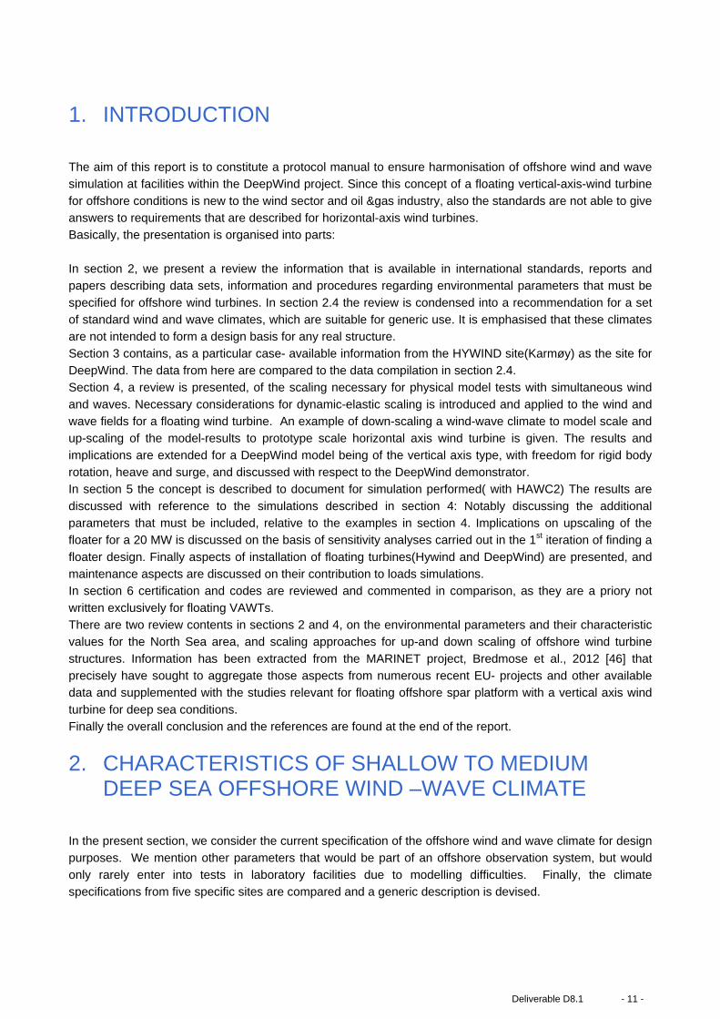
locations are shown in Figure 2.1.2.
- 12 - Deliverable D8.1
Figure 2.1.2. Full overview of locations referred to in this report, The sites are: IJmuiden:1, K13:2, Beatrice:3 and Södra Midsjöbanke: 4. For the two first see the more detailed figure 2.1.1.
The wind and wave data presented in this study thus provide examples from sites in the North Sea and Baltic Sea and further illustrate the variability between the locations. For some parameters and relations, notable similarities are observed and might thus represent general climate characteristics with wider
applicability. Here, however, it must be emphasized that the applicability of such general relations are only valid to the extent that no explicit and implicit assumptions of the applied models are violated. Examples of such violating aspects could be depth limitations, wave refraction, fetch conditions for wind generation of
waves and inadequate wind shear description. The discussion follows to a wide extent the guidelines from the EU-MARINET-project[[46.] ].
With the above in mind, for full design basis activities, the importance of site specific data cannot be over-stated. In this context, an obvious miss in the data sets from a European climate point of view, are data from the Atlantic West coast, and from the Mediterranean, as well as the Baltic Sea with ice probabilities.
Both because of the different wind and wave climate ruling there and because of the practical needs for considerations about drift ice and icing due to spray. Additional sites outside Europe would also make out a relevant extension of the study, as many European entrepreneurs are active players in the now worldwide
expansion of offshore wind energy. Specifically in connection with the DeepWind project data from the Norwegian west coast would have been useful, see 3.
In spite of these reservations, we have still chosen the UpWind design basis [[1.] ] as the basic illustrative data for this report, because it is a recent, large, comprehensive and accessible data base.
2.2 Parameters for wind and wave specification
The core part of the design basis for an offshore wind farm consists of data for the wind and wave climate. The wind characteristics of a given site can be determined from multiyear measurements of wind speed and
Deliverable D8.1 - 13 -

wind direction, preferably at several heights. Similar and simultaneous time series for the height and direction of the surface waves must be established.
The wind climate is characterised by
• mean speed • wind direction • wind shear • turbulence standard deviation and turbulence intensity • turbulence frequency spectrum • extreme wind speed with 1 year and 50 year return period.
The wind measurements must be accompanied by measuring height, z, averaging time, often 10 min averages, sampling time, often 10min)
The wave climate is characterised by • significant wave height, Hs ( standard derived on basis of 3 hours data) • peak period, Tp. • wave direction • frequency spectrum • directional distribution • misalignment (relative to the wind direction) distribution • extreme value of Hs with Tp, and the derived heights, HSmax, and HSred ( with 1 and 50 year return
period)
The multi-dimensional distribution function for these parameters must be considered to evaluate the design.
Normally one can simplify the approach considerably, using physical and statistical knowledge. This is illustrated below; we discuss the climate conditions as function of one parameter only, the wind speed. The basis for this approach is that the mean wind speed is the most important parameter to characterise both the
wind turbulence and the wave field. Additional information like water depth, tides, currents and temperature in air and water must be monitored at
the measuring site too. This information is available in the data of the UpWind design basis [1] project along with information on marine growth and bottom soil features. Finally we note that the occurrence of water ice and icing, with associated loads, should be considered in relevant regions. This was not relevant, however,
for the UpWind sites. Our approach is to seek for robust correlations between the wind and wave parameters important for the
evaluation of both fatigue and extreme loads on offshore wind turbine structures. In order to do so, we start by summarising a simplified offshore climate driven by the wind speed in the next section.
2.3 One –parameter climate based on wind speed.
In this section we seek to describe the design and load parameters for offshore wind turbines, both with respect to wind and other atmospheric parameters and with respect to the surface waves and other characteristic water parameters. A one-parameter approach is presented, where the wind speed is
considered a free parameter and all the other quantities are described conditionally to the wind speed. In the following, the parameters of this description and their typical distributions are summarized.
- 14 - Deliverable D8.1
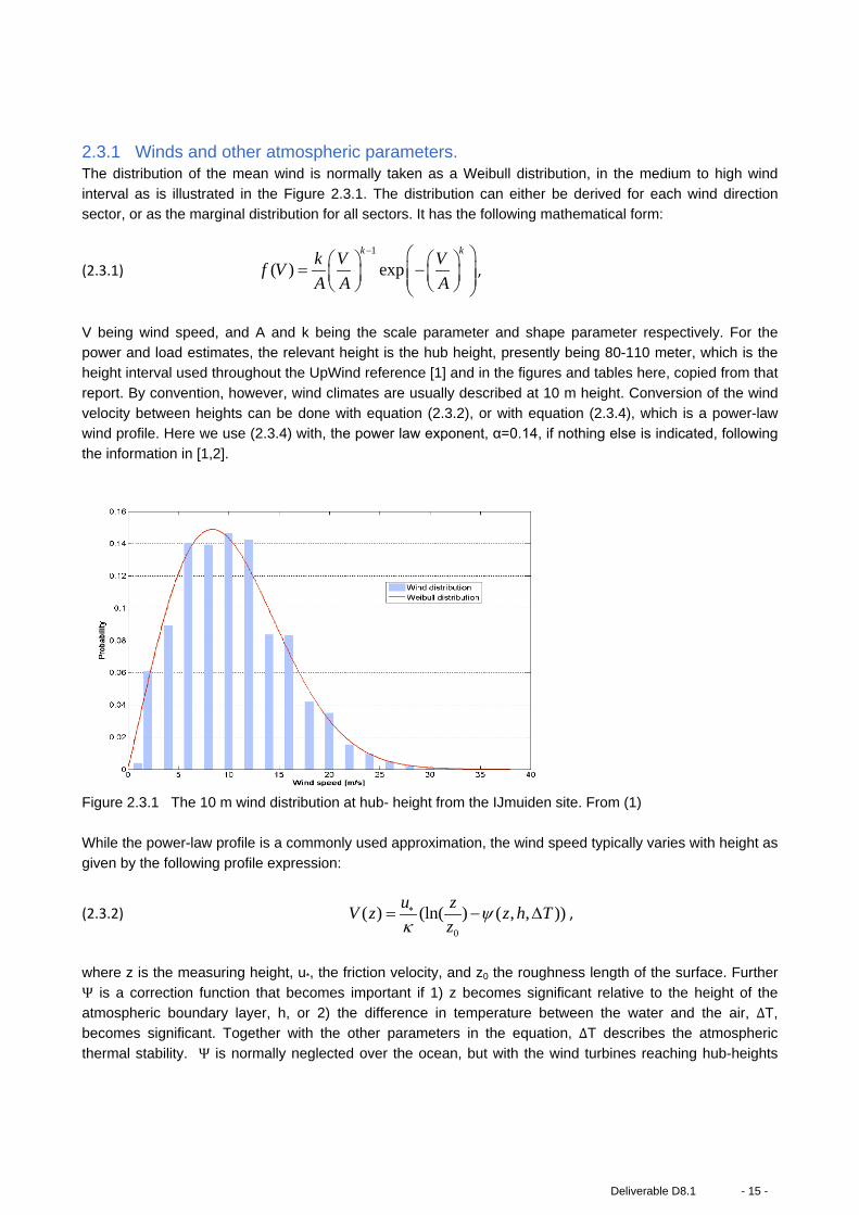
2.3.1 Winds and other atmospheric parameters. The distribution of the mean wind is normally taken as a Weibull distribution, in the medium to high wind
interval as is illustrated in the Figure 2.3.1. The distribution can either be derived for each wind direction sector, or as the marginal distribution for all sectors. It has the following mathematical form:
(2.3.1) 1
( ) expk kk V Vf V
A A A
− = − ,
V being wind speed, and A and k being the scale parameter and shape parameter respectively. For the power and load estimates, the relevant height is the hub height, presently being 80-110 meter, which is the height interval used throughout the UpWind reference [1] and in the figures and tables here, copied from that
report. By convention, however, wind climates are usually described at 10 m height. Conversion of the wind velocity between heights can be done with equation (2.3.2), or with equation (2.3.4), which is a power-law wind profile. Here we use (2.3.4) with, the power law exponent, α=0.14, if nothing else is indicated, following
the information in [1,2].
Figure 2.3.1 The 10 m wind distribution at hub- height from the IJmuiden site. From (1) While the power-law profile is a commonly used approximation, the wind speed typically varies with height as
given by the following profile expression:
(2.3.2) 0
( ) (ln( ) ( , , ))u zV z z h T
zψ
κ∗= − ∆ ,
where z is the measuring height, u*, the friction velocity, and z0 the roughness length of the surface. Further
Ψ is a correction function that becomes important if 1) z becomes significant relative to the height of the atmospheric boundary layer, h, or 2) the difference in temperature between the water and the air, ∆T, becomes significant. Together with the other parameters in the equation, ∆T describes the atmospheric
thermal stability. Ψ is normally neglected over the ocean, but with the wind turbines reaching hub-heights
Deliverable D8.1 - 15 -
larger than 100m, it may not be defensible anymore. As this subject is still under active research and is not yet included in the design standards, Ψ= 0 is assumed throughout the present report.
The roughness height z0 can be determined from Charnock’s relation: (2.3.3) 2
0 /z Cu g∗= ,
where C is a coefficient between 0.01 and 0.015, dependent on the nearness of a coast (and to some extent also on wind and wave history), and g is the acceleration due to gravity. Over water, z0 is a small quantity, of the order of 0.1-0.3 mm.
As an alternative to the log-law above one can use the so called power law profile given by (2.3.4) 10 10( ) ( )( / )V z V z z z α= ,
The power law coefficient α is taken as 0.14 in the UpWind design basis [1], which is also recommended in [2], but by comparison with the log-expression (2.3.2) it is seen that it will vary with z0 and ∆T and also the z-
interval used. This variation is neglected in most guideline and standard literature. Here it will show up together with the statistical scatter around the average behaviour. However, from both (2.3.2) and (2.3.4 with variable α), it is seen that the Weibull distribution must change both A and k with height, not only A, as would
be the case with a constant α. Indeed closer studies show that typically k will increase from its value at 10m with height up to around 80m followed by a gradual decrease further up [16], showing a maximum variation of 0.5 across the boundary layer, However, this is presently under research. In the present simplified
description, the Weibull k parameter is therefore taken to be independent with height, consistent with the choice of a constant value of α.
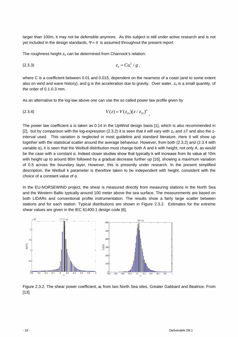
In the EU-NORSEWIND project, the shear is measured directly from measuring stations in the North Sea and the Western Baltic typically around 100 meter above the sea surface. The measurements are based on both LIDARs and conventional profile instrumentation. The results show a fairly large scatter between
stations and for each station. Typical distributions are shown in Figure 2.3.2. Estimates for the extreme shear values are given in the IEC 61400-1 design code [6].
Figure 2.3.2. The shear power coefficient, 𝛂𝛂, from two North Sea sites, Greater Gabbard and Beatrice. From [13].
- 16 - Deliverable D8.1
Using the expressions of (2.3.2) or (2.3.4) one can refer the 10-meter wind speed to hub-height, which is the speed normally used in connection with design studies. As seen from the figure a good deal of variability in the extrapolation must be expected due to the variability of the power coefficient. Equation (2.3.2) illustrates
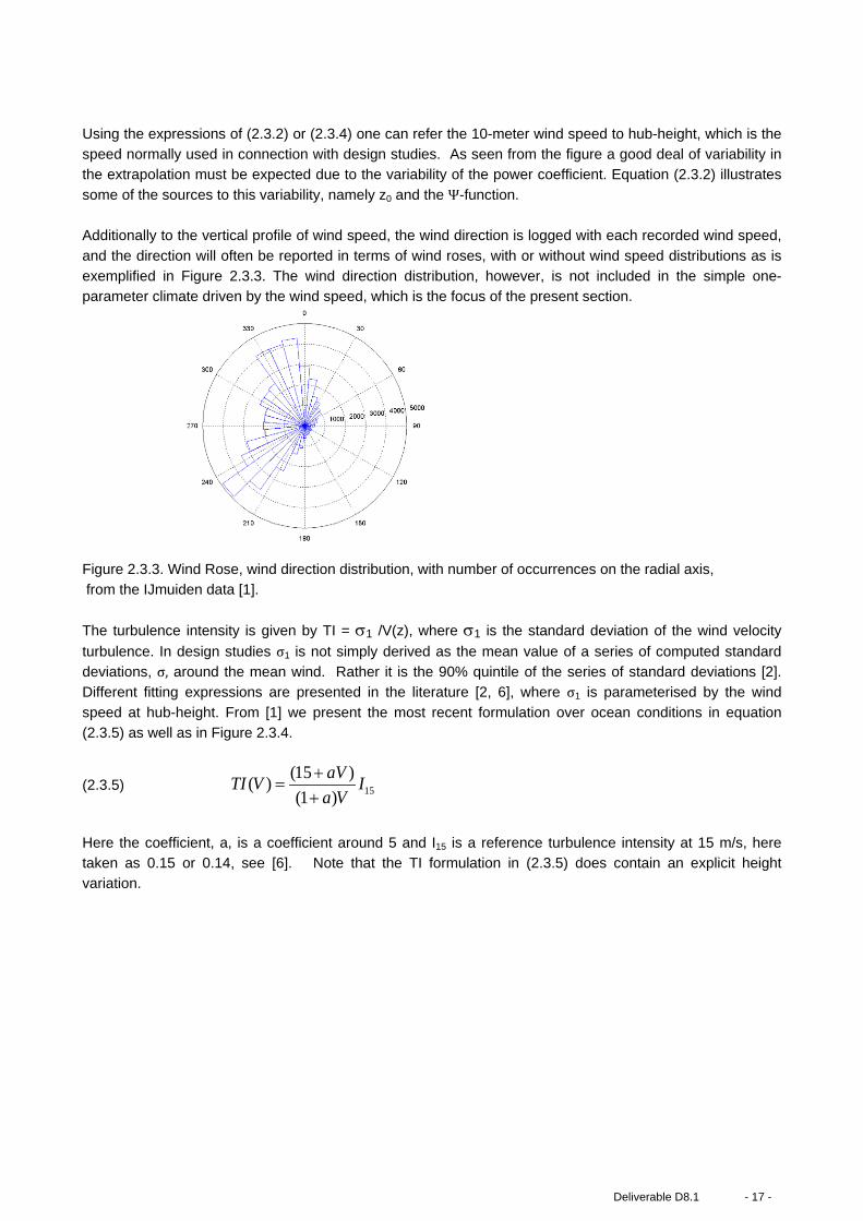
some of the sources to this variability, namely z0 and the Ψ-function. Additionally to the vertical profile of wind speed, the wind direction is logged with each recorded wind speed,
and the direction will often be reported in terms of wind roses, with or without wind speed distributions as is exemplified in Figure 2.3.3. The wind direction distribution, however, is not included in the simple one-parameter climate driven by the wind speed, which is the focus of the present section.
Figure 2.3.3. Wind Rose, wind direction distribution, with number of occurrences on the radial axis, from the IJmuiden data [1].
The turbulence intensity is given by TI = σ1 /V(z), where σ1 is the standard deviation of the wind velocity
turbulence. In design studies σ1 is not simply derived as the mean value of a series of computed standard deviations, σ, around the mean wind. Rather it is the 90% quintile of the series of standard deviations [2]. Different fitting expressions are presented in the literature [2, 6], where σ1 is parameterised by the wind
speed at hub-height. From [1] we present the most recent formulation over ocean conditions in equation (2.3.5) as well as in Figure 2.3.4.
(2.3.5)
15
(15 )( )
(1 )
aVTI V Ia V+
=+
Here the coefficient, a, is a coefficient around 5 and I15 is a reference turbulence intensity at 15 m/s, here taken as 0.15 or 0.14, see [6]. Note that the TI formulation in (2.3.5) does contain an explicit height variation.
Deliverable D8.1 - 17 -

Figure 2.3.4. Turbulence Intensity at hub-height according UpWind, IEC (1,2,6). From [1]. For lower wind speeds, σ and σ1 (the 90% quantile) do not decrease as fast as V(z) for decreasing wind and
TI increases for decreasing wind. For larger winds TI reaches a limit value, or does actually increase a little , due to an increasing z0 with u* as given by the Charnock relation (2.3.3). Although we have here specified both the wind shear and the turbulence intensity as analytical functions of V, they will appear with statistical scatter around these expected values, when they are based on direct measurements. Further to the normal turbulence defined by (2.3.5) one can also specify an extreme turbulence intensity for certain load studies, see Figure 2.3.4. Turbulence can be characterised by the frequency spectrum, S(f), of the horizontal wind speed, scaling with
the turbulence standard deviation, σ, and it’s spatial and temporal scales. The literature shows several forms that have a great deal of overlap as they all represent the same atmospheric physics, with similar combinations of data fitting and theory. Here we cite the Kaimal form as presented in [3]:
(2.3.6) 2 10
5/3
10
4
( )(1 6 )
LfVfS f LfV
σ=+
,
where f is frequency (Hz), σ is the standard deviation of the turbulence and L is the characteristic turbulence
length scale, taken as:
(2.3.7) 5.67 60
340.2 60
z for z mLfor z m
<= >
The turbulence spectrum above describes the frequency distribution as well the wave number spectrum,
because the atmospheric turbulence to a good approximation obey Taylors hypothesis of frozen turbulence, meaning that f= VkV/2π, where kV is the wave number along the mean wind direction.
- 18 - Deliverable D8.1
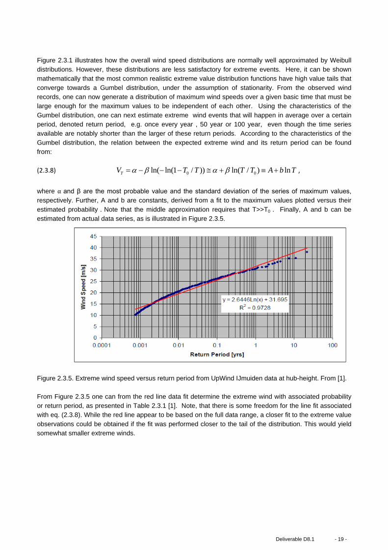
Figure 2.3.1 illustrates how the overall wind speed distributions are normally well approximated by Weibull distributions. However, these distributions are less satisfactory for extreme events. Here, it can be shown mathematically that the most common realistic extreme value distribution functions have high value tails that
converge towards a Gumbel distribution, under the assumption of stationarity. From the observed wind records, one can now generate a distribution of maximum wind speeds over a given basic time that must be large enough for the maximum values to be independent of each other. Using the characteristics of the
Gumbel distribution, one can next estimate extreme wind events that will happen in average over a certain period, denoted return period, e.g. once every year , 50 year or 100 year, even though the time series available are notably shorter than the larger of these return periods. According to the characteristics of the
Gumbel distribution, the relation between the expected extreme wind and its return period can be found from:
(2.3.8) 0 0ln( ln(1 / )) ln( / ) lnTV T T T T A b Tα β α β= − − − ≅ + ≡ + ,
where α and β are the most probable value and the standard deviation of the series of maximum values, respectively. Further, A and b are constants, derived from a fit to the maximum values plotted versus their
estimated probability . Note that the middle approximation requires that T>>T0 . Finally, A and b can be estimated from actual data series, as is illustrated in Figure 2.3.5.
Figure 2.3.5. Extreme wind speed versus return period from UpWind IJmuiden data at hub-height. From [1].
From Figure 2.3.5 one can from the red line data fit determine the extreme wind with associated probability or return period, as presented in Table 2.3.1 [1]. Note, that there is some freedom for the line fit associated with eq. (2.3.8). While the red line appear to be based on the full data range, a closer fit to the extreme value
observations could be obtained if the fit was performed closer to the tail of the distribution. This would yield somewhat smaller extreme winds.
Deliverable D8.1 - 19 -
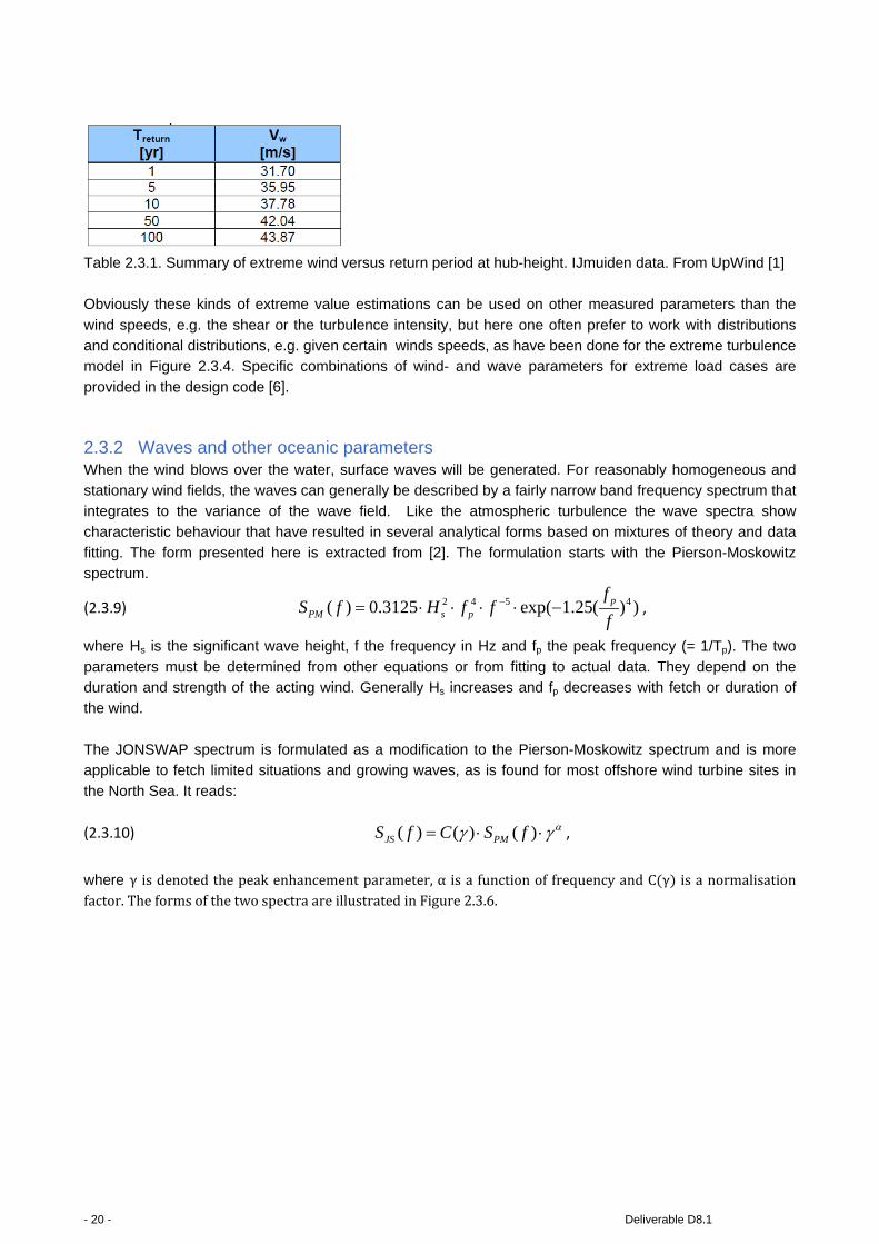
Table 2.3.1. Summary of extreme wind versus return period at hub-height. IJmuiden data. From UpWind [1] Obviously these kinds of extreme value estimations can be used on other measured parameters than the
wind speeds, e.g. the shear or the turbulence intensity, but here one often prefer to work with distributions and conditional distributions, e.g. given certain winds speeds, as have been done for the extreme turbulence model in Figure 2.3.4. Specific combinations of wind- and wave parameters for extreme load cases are
provided in the design code [6]. 2.3.2 Waves and other oceanic parameters When the wind blows over the water, surface waves will be generated. For reasonably homogeneous and stationary wind fields, the waves can generally be described by a fairly narrow band frequency spectrum that
integrates to the variance of the wave field. Like the atmospheric turbulence the wave spectra show characteristic behaviour that have resulted in several analytical forms based on mixtures of theory and data fitting. The form presented here is extracted from [2]. The formulation starts with the Pierson-Moskowitz
spectrum.
(2.3.9) 2 4 5 4( ) 0.3125 exp( 1.25( ) )pPM s p
fS f H f f
f−= ⋅ ⋅ ⋅ ⋅ − ,
where Hs is the significant wave height, f the frequency in Hz and fp the peak frequency (= 1/Tp). The two
parameters must be determined from other equations or from fitting to actual data. They depend on the duration and strength of the acting wind. Generally Hs increases and fp decreases with fetch or duration of the wind.
The JONSWAP spectrum is formulated as a modification to the Pierson-Moskowitz spectrum and is more applicable to fetch limited situations and growing waves, as is found for most offshore wind turbine sites in
the North Sea. It reads: (2.3.10) ( ) ( ) ( )JS PMS f C S f αγ γ= ⋅ ⋅ ,
where γ is denoted the peak enhancement parameter, α is a function of frequency and C(γ) is a normalisation factor. The forms of the two spectra are illustrated in Figure 2.3.6.
- 20 - Deliverable D8.1

Figure 2.3.6. Sketch of the wave spectrum according to the Pierson-Moskowitz spectrum and according to the JONSWAP spectrum. From [9]. For γ →1 the Pierson-Moskowitz spectrum is recovered. Formulas for α and C are provided in [2]. The value of γ is often taken to be γ =3.3 for storm waves and γ=1.0 for fatigue calculations. It can also be estimated with basis in the spectral parameters [6] where Hs must be inserted in metres and Tp in seconds: (2.3.11) Even for a constant wind speed of wind direction θ0, all waves do not propagate along the wind direction, but in an angle interval around θ0. This is normally expressed by a directional wave spectrum [2,15] , for example the ‘cosine 2s spectrum’
(2.3.12) 0( , ) ( ) ( , ), ( , ) cos ( )sS f S f D f with D fθ θ θ θ θ= ⋅ ≈ − .
Here D(f,θ) normalises to 1 by integration over θ, and s is described by a complex function of f and the
characteristics of the spectral function in (2.3.11), see [15]. Another reason for waves propagating in different directions from the local wind is that the wind is neither
homogenous nor stationary, and waves generated at other times and places may propagate across the measuring site following the direction of the wind, when and where they were formed. They will typically appear at the lower frequency end of the locally generated SJS(f) spectrum, because long waves dissipate
slower than short waves. They are denoted swells, and will at some sites be significant.
Deliverable D8.1 - 21 -
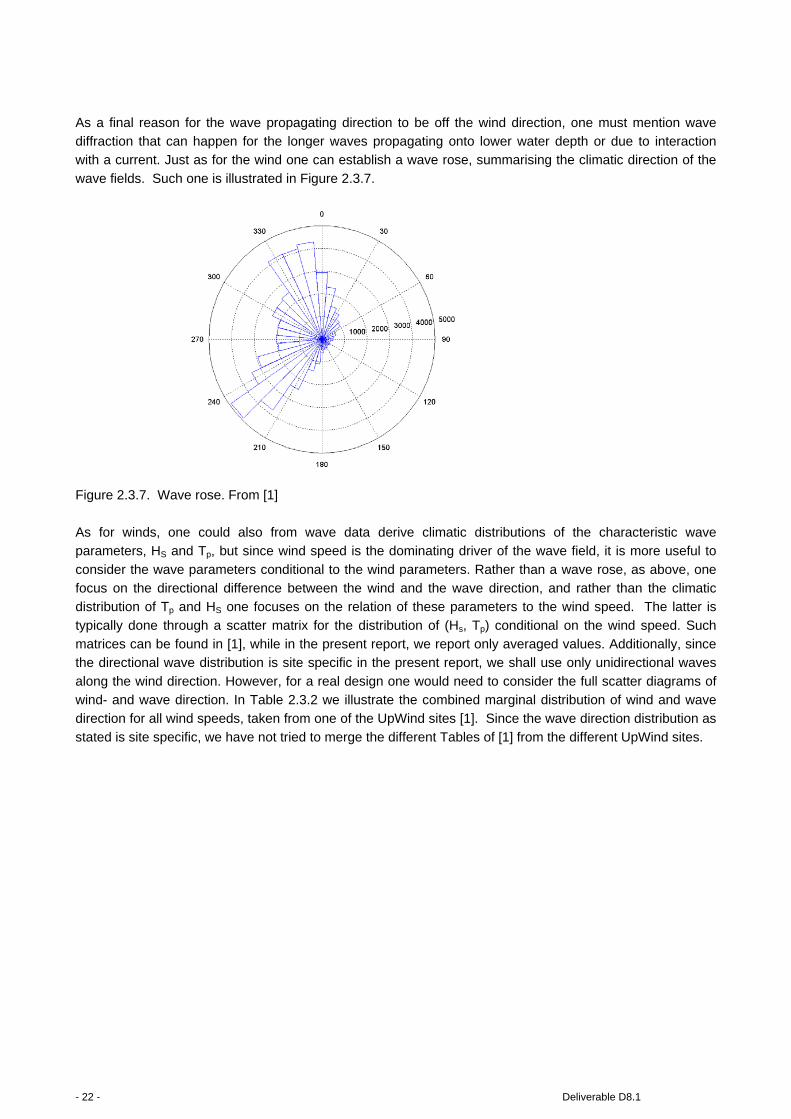
As a final reason for the wave propagating direction to be off the wind direction, one must mention wave diffraction that can happen for the longer waves propagating onto lower water depth or due to interaction with a current. Just as for the wind one can establish a wave rose, summarising the climatic direction of the
wave fields. Such one is illustrated in Figure 2.3.7.
Figure 2.3.7. Wave rose. From [1]
As for winds, one could also from wave data derive climatic distributions of the characteristic wave parameters, HS and Tp, but since wind speed is the dominating driver of the wave field, it is more useful to
consider the wave parameters conditional to the wind parameters. Rather than a wave rose, as above, one focus on the directional difference between the wind and the wave direction, and rather than the climatic distribution of Tp and HS one focuses on the relation of these parameters to the wind speed. The latter is
typically done through a scatter matrix for the distribution of (Hs, Tp) conditional on the wind speed. Such matrices can be found in [1], while in the present report, we report only averaged values. Additionally, since the directional wave distribution is site specific in the present report, we shall use only unidirectional waves
along the wind direction. However, for a real design one would need to consider the full scatter diagrams of wind- and wave direction. In Table 2.3.2 we illustrate the combined marginal distribution of wind and wave direction for all wind speeds, taken from one of the UpWind sites [1]. Since the wave direction distribution as
stated is site specific, we have not tried to merge the different Tables of [1] from the different UpWind sites.
- 22 - Deliverable D8.1

Table 2.3.2. Distribution of simultaneous propagation directions for wind and waves, taken from the K13 site in UpWind. Taken from [1].
2.3.3 Lumped wind-wave climate for fatigue calculation While the full wind-wave climate at a site is a multi-dimensional parameter space with a multi-dimensional
statistical distribution function, it can be practically expressed in terms of a one-parameter climate conditional to the wind speed. In this approach, central values of all other parameters are determined by suitable averaging through the parameter space. The overall purpose of such a simpler climate description is to
simplify the fatigue calculations for the structure. Therefore, the averaging of the climate parameters is done with respect to fatigue contribution and not simply with respect to probability of occurrence. An example of such a lumped wind-wave climate is given in Table 2.3.3 which shows the wave and wind parameters as
function of mean wind speed at hub height together with the frequency of occurrence for each wind speed bin. The statistics in the table are lumped according to the method of Kühn [1, 43]. Two turbulence intensity values are shown, namely those associated with the normal and extreme turbulence models, see [1]. It
should be emphasized that the estimates of turbulence intensity are derived from the normal turbulence model used also in Figure 2.3.4 and in (2.3.4), based on assumptions about the distribution of TI for a given wind speed.
The two γ-values of 1.0 and 3.3 are quite usual, and we shall return to this in section 2.4. Finally, we point out that HS and Tp values are weighted values for a given wind speed. Individual values will scatter statistical
around these averages. It should be mentioned that the fatigue-weighting of the wave data cited here was done for bottom fixed wind
turbines. Hence, for a floating wind turbine, the weighting is likely to be different and might thus lead to other weighted values of Hs and Tp. Currently an extensive study is conducted by NREL, University of
Deliverable D8.1 - 23 -

Massachusetts, and University of Stuttgart to address this question. A numerous set of aero-elastic simulations (1-2 million of 10min duration) has been made and will be used to establish a recommendation for simplifying load cases for extreme and fatigue calculations for floating wind turbines. First results from the
study were presented at OMAE 2013: “L. Haid, G. Stewart, Jason Jonkman, Matthew Lackner, Denis Matha, Amy Robertson ‘Simulation-Length Requirements in the Loads Analysis of Offshore Floating Wind Turbines’ ”.
Table 2.3.3. Lumped wind-wave climate conditional to wind speed at hub height (here 85 meter above mean sea level). The table provides turbulence intensities, significant wave height, period of the peak frequency,
and peaked-ness for the wave spectrum, probability of occurrence, or correspondingly duration of occurrence per year. Data are from the K13 site from the UpWind project [1]. 2.3.4 Extreme values for wave climate The lumped statistics of data in the table above is very suitable for fatigue load studies. For the extreme loads one must use the extreme values of both winds and wave heights as estimated by the Gumbel
statistics in the text above, corresponding to a 1 year and 50 year return period. This is illustrated in figure 2.3.8, also taken from the K13 site in the UpWind report [1].
- 24 - Deliverable D8.1

Figure 2.3.8. Extreme HS versus return period by the Gumbel method for the K13 shallow depth site of UpWind. From [1].
From Figure (2.3.8), we can summarise the extreme waves as function of the return period:
Table 2.3.4. Extreme significant wave heights as derived from the Gumbel corresponding to the UpWind K13 shallow depth site. From [1].
The HS- value is taken directly from the Gumbel fit method of the Figure 2.3.8. Similar remarks as for Figure 2.3.5 on the range of line-fitting and the implication for the extreme values of Table 2.3.4 apply. Hmax is based on that HS is derived from an average over 3 hours and that the waves are Rayleigh distributed, giving
rise to a maximum value being ~ 1.86 times HS [2]. The peak period corresponding to the extreme wind speeds must be bounded by the following formula criterion, [2]:
(2.3.12) 11.1 ( ) / 14.3 ( ) /S SH U g T H U g≤ ≤ ,
where one should select the peak period that results in the strongest loads.
Deliverable D8.1 - 25 -

2.4 Standard offshore conditions for testing and modelling In this section we extract a set of offshore standard conditions for test and modelling. The extraction is made
from data of the UpWind design basis and from the Beatrice and Södra Midsjöbank sites. 2.4.1 Wind climate parameters in the extended North Sea and Baltic Sea The wind conditions over the extended North Sea and Baltic Sea is illustrated in Figure 2.4.1 and 2.4.2 taken from the EU-NORTHWIND reporting [13, 14] on the marine winds of NW Europe. Figure 2.4.1 shows the mesoscale modelling result of the average 100 meter wind speed 2006-11, while the four plots of Figure
2.4.2 depicts the marine wind climate at 10 meter height measured by radar from 10 year satellite measurements [14]. The figures illustrate the variability of wind parameters in the extended North Sea and Baltic Sea.
Figure 2.4.1 The variation of the 100 m mean wind across the NorthWestern European waters, as modelled by mesoscale modelling, Norsewind. From [13].
- 26 - Deliverable D8.1

Figure 2.4.2 The 10 meter marine wind climate across the North Western European seas. The white areas correspond to lack of data, mainly due to precipitation. From [14].
The figures indicate that one should expect a fairly gradual change in the wind characteristic of the North Western European waters, with exception of the quite close to coastal areas. At 10 m above the surface, a typical Weibull A parameter is seen to be about 9 m/s, with a k-value about 2. The A and k--value seems of
the order of the ones derived from the 10m distributions in Figure 2.4.3 and presented in Table 2.4.1. 2.4.2 Wind and wave climate for five specific sites We now compare the wind and wave climate parameters for five sites, namely the three sites of the UpWind design basis, the Beatrice site and Södra Midsjöbanken. The UpWind data are extracted from [1], while the Beatrice and Södra Midsjöbanken results are taken from [10,11]. It should be noted that the wave data from
Södra Midsjöbanken are not based on measurements but have been calculated with closed-form wave growth models. The analysis is taken from[[46.] ]
A first summary is provided in Table 2.4.3 which lists the Weibull wind distribution parameters, the extreme (1,50)-year wind speed and significant wave heights, the water depth and the lumped wave climate parameters for V10= 20m/s. Given the difference in geographical location, the similarity between the wind and
Deliverable D8.1 - 27 -

wave parameters is quite remarkable. Further, the 10 meter A and k values of the table compare quite well with the satellite data of Figure 2.4.2.
Table 2.4.1 Summary of parameters from the 5 sites considered. Note that the wave parameters from Södra Midsjöbanken are modelled and not based on measurements. On the K13 Deep site, the depth is indicated by “50”, because of the way the K13 Deep data set is made, see section 2.1. The HS and Tp data from
Södra Midsjöbanken are marked with “ “ also, because they are based on wave growth models not data. At Beatrice and Södra Midsjöbanken no other extreme values than the 50-year wind speed were determined
Site A10 K HS
V10= 20m/s
Tp,
V10= 20m/s
V50
m/s
V1
m/s
HS,50
m
HS,1
M
Depth
m
IJmuiden 7.9 2.1 4.2 8.7 31.5 23.8 7.6 5.7 21
K13 shallow 9.3 2.0 3.5 8.0 34.1 25.9 8.2 6.1 25
K13 Deep 9.3 2.1 3.5 8.0 34.1 25.9 9.4 7.1 50
Beatrice 8.7 1,9 3.8 6.5 38.5 - - - 44
Södra Midsjöbanken 8.2 2.1 3.3 7.5 35.2 - - - 15
Next, two tables of lumped wind-wave climates are provided in Table 2.4.2 and 2.4.3, pertaining to the
IJmuiden shallow water site and the K13 shallow water site. The similar table for the K13 deep water site (not shown here) is identical to the one of the K13 shallow water side except for 1) the probabilities, which are associated with the difference in the Weibull parameters for the wind speed distribution at the two sites;
and 2) the extreme wave data, which are not listed in these tables. Table 2.4.2 Lumped statistics from the IJjmuiden site. The wind speed refers to the hub height (83.9 m).
From [1].
- 28 - Deliverable D8.1

Table 2.4.3 Lumped statistics from the K13 shallow site. The wind speed refers to the hub height (85.2 m). From [1]
The similarity and differences between the different sites are now analysed in terms of graphical comparison. Figure 2.4.3 shows the wind distributions together with raw data and the fitted Weibull distributions. The Weibull parameters are those of Table 2.4.1. In general a reasonable match to the Weibull curve is
observed. Further, as is also reflected by the similarity of the Weibull parameters in Table 2.4.1, the wind distributions from the different sites are fairly similar.
Figure 2.4.3 The 10 m wind speed distribution at the 5 sites considered, compared to a each other and an
analytical Weibull function.
Deliverable D8.1 - 29 -
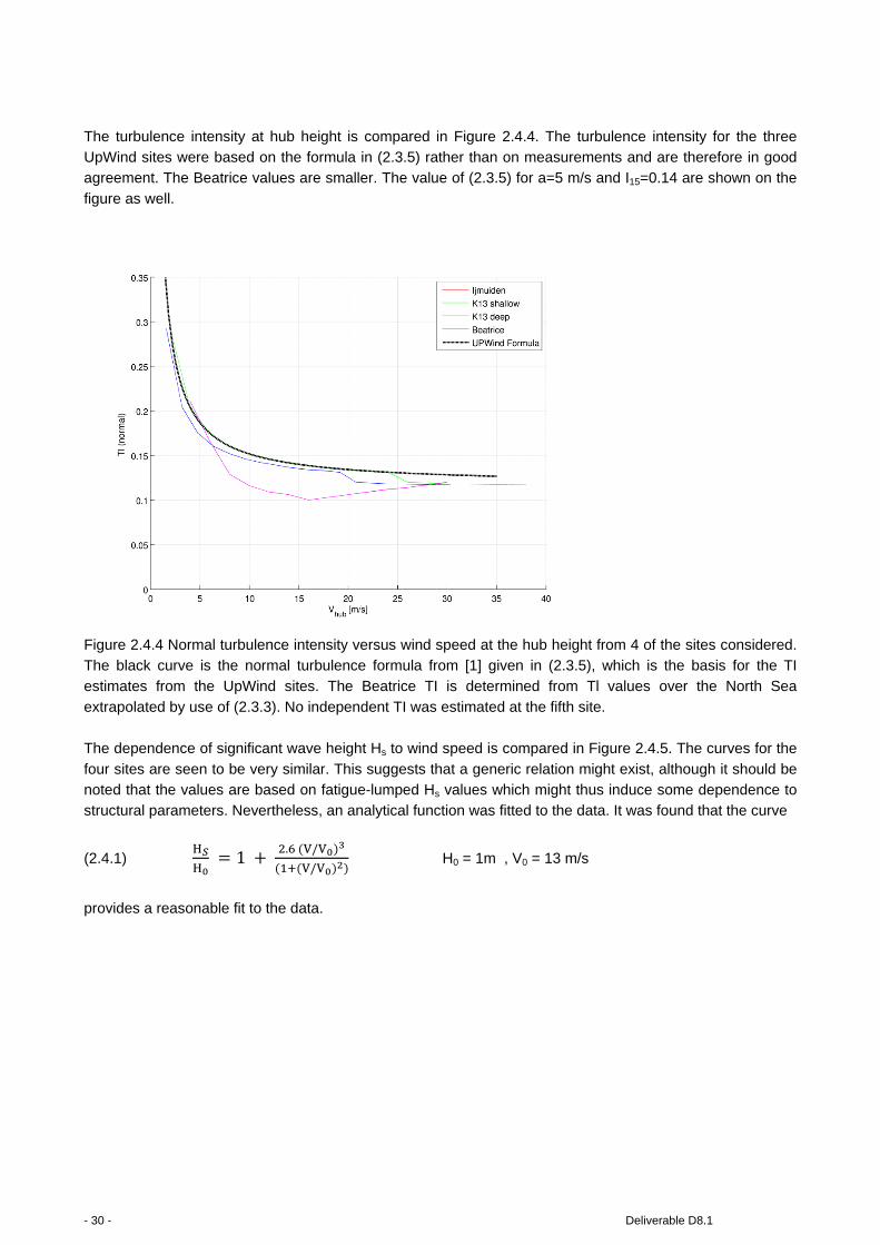
The turbulence intensity at hub height is compared in Figure 2.4.4. The turbulence intensity for the three UpWind sites were based on the formula in (2.3.5) rather than on measurements and are therefore in good agreement. The Beatrice values are smaller. The value of (2.3.5) for a=5 m/s and I15=0.14 are shown on the
figure as well.
Figure 2.4.4 Normal turbulence intensity versus wind speed at the hub height from 4 of the sites considered. The black curve is the normal turbulence formula from [1] given in (2.3.5), which is the basis for the TI estimates from the UpWind sites. The Beatrice TI is determined from Tl values over the North Sea
extrapolated by use of (2.3.3). No independent TI was estimated at the fifth site. The dependence of significant wave height Hs to wind speed is compared in Figure 2.4.5. The curves for the
four sites are seen to be very similar. This suggests that a generic relation might exist, although it should be noted that the values are based on fatigue-lumped Hs values which might thus induce some dependence to structural parameters. Nevertheless, an analytical function was fitted to the data. It was found that the curve
(2.4.1) H𝑆H0
= 1 + 2.6 (V/V0)3
(1+(V/V0)2) H0 = 1m , V0 = 13 m/s
provides a reasonable fit to the data.
- 30 - Deliverable D8.1
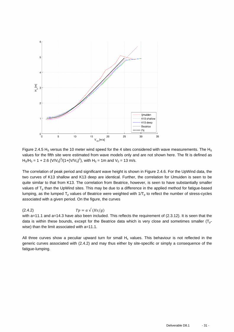
Figure 2.4.5 HS versus the 10 meter wind speed for the 4 sites considered with wave measurements. The HS values for the fifth site were estimated from wave models only and are not shown here. The fit is defined as HS/H0 = 1 + 2.6 (V/V0)
3/(1+(V/V0)2), with H0 = 1m and V0 = 13 m/s.
The correlation of peak period and significant wave height is shown in Figure 2.4.6. For the UpWind data, the two curves of K13 shallow and K13 deep are identical. Further, the correlation for IJmuiden is seen to be
quite similar to that from K13. The correlation from Beatrice, however, is seen to have substantially smaller values of Tp than the UpWind sites. This may be due to a difference in the applied method for fatigue-based lumping, as the lumped Tp values of Beatrice were weighted with 1/Tp to reflect the number of stress-cycles
associated with a given period. On the figure, the curves (2.4.2) 𝑇𝑝 = 𝑎 √ (𝐻𝑠/𝑔)
with a=11.1 and a=14.3 have also been included. This reflects the requirement of (2.3.12). It is seen that the data is within these bounds, except for the Beatrice data which is very close and sometimes smaller (Tp-wise) than the limit associated with a=11.1.
All three curves show a peculiar upward turn for small Hs values. This behaviour is not reflected in the generic curves associated with (2.4.2) and may thus either by site-specific or simply a consequence of the
fatigue-lumping.
Deliverable D8.1 - 31 -

Figure 2.4.6 Tp versus HS, estimated from data at the four sites considered. For the UpWind sites (2), the data are tabulated in section 2.3. The Beatrice curve is from [10] and is on the lower bound, which may reflect the nearness of the coast at this site. The two analytical curves reflect bounds for Tp in (2.3.12).
The JONSWAP peak enhancement parameter, γ, is determined from (2.3.11) and depicted in figure 2.4.7. It is seen that the UpWind sea states show a general increase in γ for increasing wind speed, towards a
maximum value of approximately 2.5. The Beatrice values grow readily to a value of γ=5, which is very large. This may be explained by the relatively small Tp values, which again might be a consequence of the fatigue-lumping method rather than the actual sites wave climate.
- 32 - Deliverable D8.1
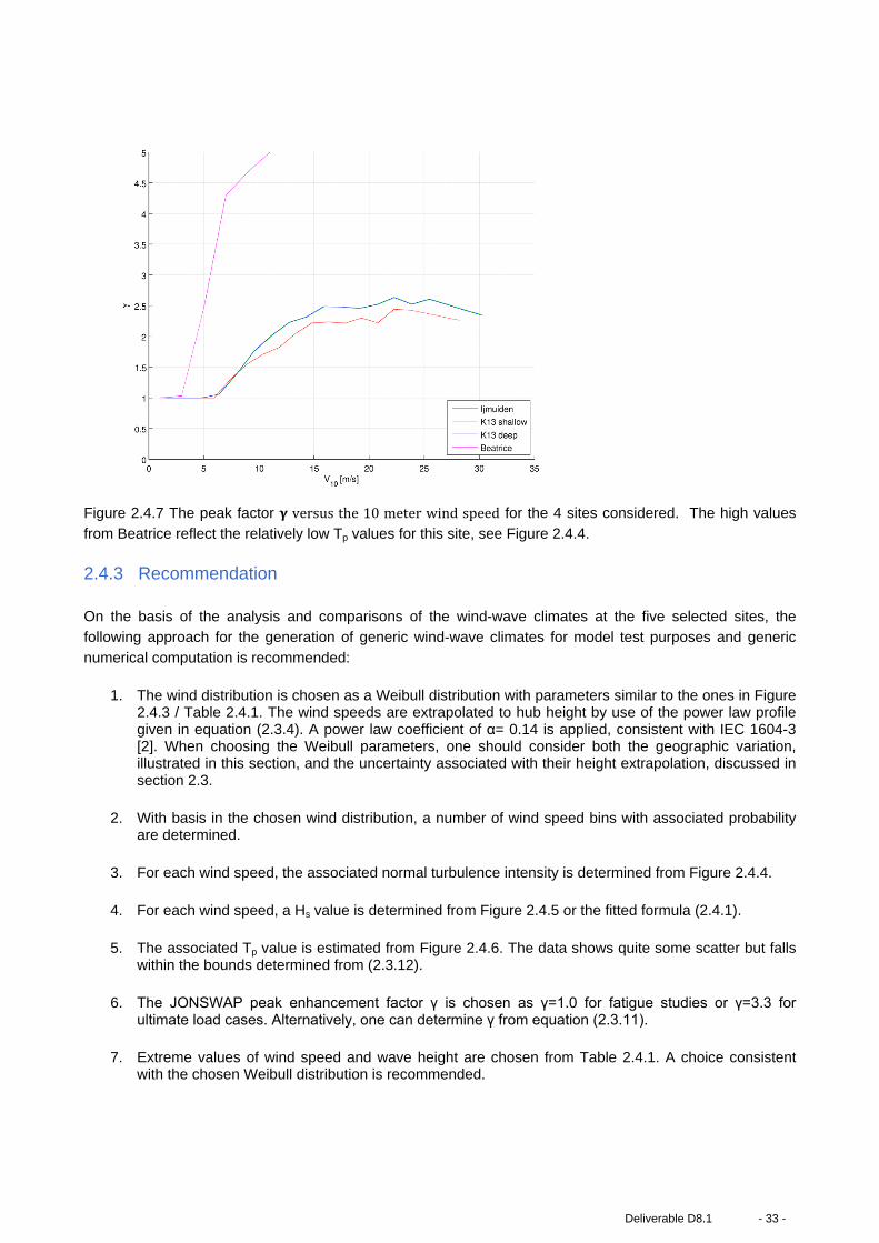
Figure 2.4.7 The peak factor 𝛄𝛄 versus the 10 meter wind speed for the 4 sites considered. The high values from Beatrice reflect the relatively low Tp values for this site, see Figure 2.4.4. 2.4.3 Recommendation On the basis of the analysis and comparisons of the wind-wave climates at the five selected sites, the
following approach for the generation of generic wind-wave climates for model test purposes and generic numerical computation is recommended:
1. The wind distribution is chosen as a Weibull distribution with parameters similar to the ones in Figure 2.4.3 / Table 2.4.1. The wind speeds are extrapolated to hub height by use of the power law profile given in equation (2.3.4). A power law coefficient of α= 0.14 is applied, consistent with IEC 1604-3 [2]. When choosing the Weibull parameters, one should consider both the geographic variation, illustrated in this section, and the uncertainty associated with their height extrapolation, discussed in section 2.3.
2. With basis in the chosen wind distribution, a number of wind speed bins with associated probability
are determined.
3. For each wind speed, the associated normal turbulence intensity is determined from Figure 2.4.4.
4. For each wind speed, a Hs value is determined from Figure 2.4.5 or the fitted formula (2.4.1).
5. The associated Tp value is estimated from Figure 2.4.6. The data shows quite some scatter but falls
within the bounds determined from (2.3.12).
6. The JONSWAP peak enhancement factor γ is chosen as γ=1.0 for fatigue studies or γ=3.3 for
ultimate load cases. Alternatively, one can determine γ from equation (2.3.11).
7. Extreme values of wind speed and wave height are chosen from Table 2.4.1. A choice consistent with the chosen Weibull distribution is recommended.
Deliverable D8.1 - 33 -
Hereby a lumped wind-wave climate is established along with extreme values for wind speed and wave height. The climates are not intended as a replacement of any real data for a specific site. But with no data available the procedure can serve to exemplify the relevant parameters and their correlation with wind
speed.
3. DEEP SEA OFFSHORE MET-OCEAN CONDITIONS-THE SITE OF DEEPWIND (SITE KARMØY)
3.1 General considerations In addition of what has been said about the wind and wave conditions, they are- inclusive currents at the Karmøy site(NO) difficult to describe quantitatively without the foundations from measurements. There are
existing forecast models of wind and waves available, which needs validation, and there are existing STATOIL proprietary measurements, for which we have given no permit to access. Through the free access to the met-ocean data from Norwegian Meteorological Institute, we downloaded standard measurements of
wind speed and direction at 10 m, and current speeds at different depths from the auto station at Utsira Fyr for the period 2010 – 2011. The values are hourly. For the information on currents and the link between waves and wind, the data are used to roughly indicate trends. For the wind part in chapter 3.4, the
measurement for the period 2009-2013 will be used to roughly validate the modeled data.
The waves are driven partially by wind shear forces in combination with forces based on oceanic effects, in particular the water laminas below the SWL is influenced by the Coriolis forces at the site. For the underwater part temperature effects plays a role, and the waves effect decay with depth, so the wind driven
Coriolis forcing, and will reduce and be taken over by particular currents affected by underwater orography, climatic forcing and a underwater Coriolis force. How strong this effect is for currents depends on the site and is not known in detail at the moment.
The SWL is the dividing line in exchange of properties between the two environments and therefore the boundary condition at SWL is common for the water surface part and the area above sea.
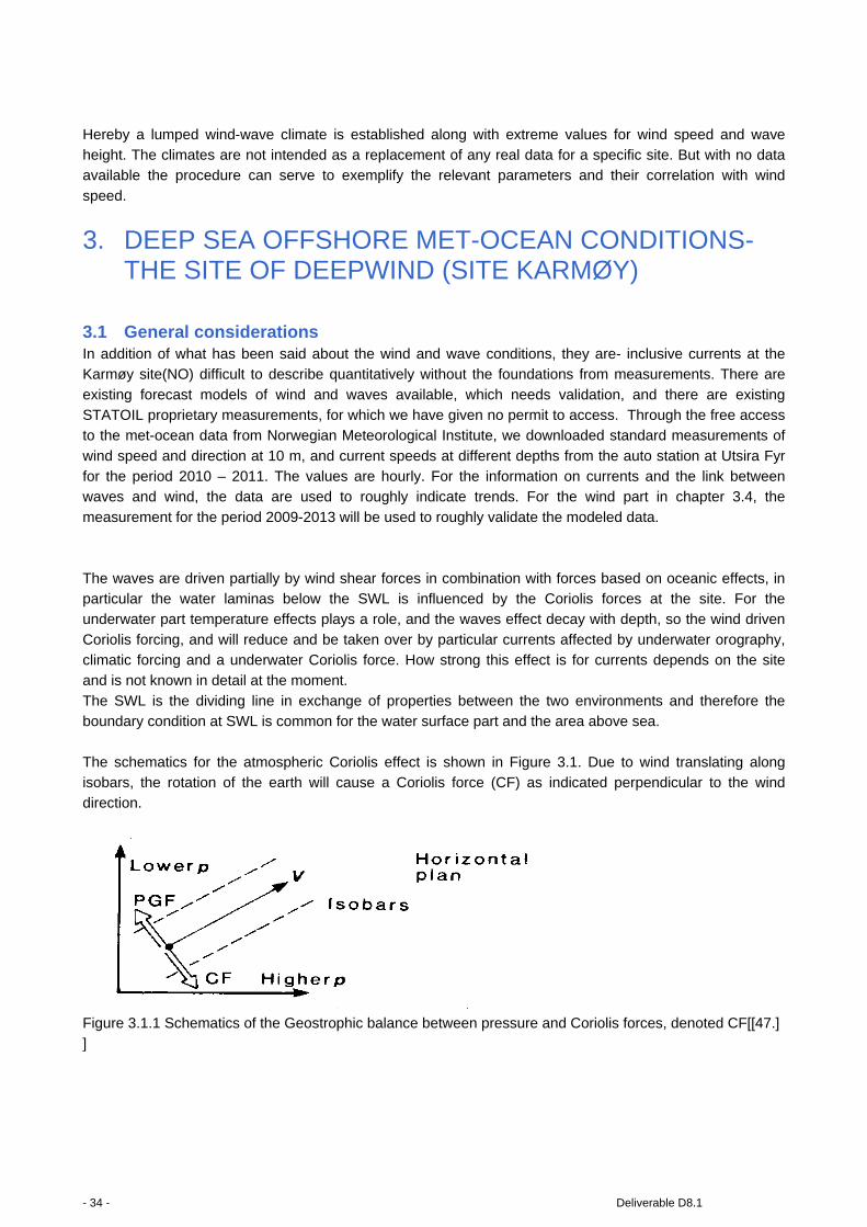
The schematics for the atmospheric Coriolis effect is shown in Figure 3.1. Due to wind translating along isobars, the rotation of the earth will cause a Coriolis force (CF) as indicated perpendicular to the wind direction.
Figure 3.1.1 Schematics of the Geostrophic balance between pressure and Coriolis forces, denoted CF[[47.] ]
- 34 - Deliverable D8.1
For the Ocean current Ekman spiral, the atmospheric Ekman layer above an ocean surface drives an ocean Ekman layer below the water line. Applying the boundary constraints between air and water, surface lamina speeds are described by the mean temporal components[[47.] ]:
(3.1)
/
/
( ) cos( / ),
( ) sin( / );
Ew
Ew
z ha EEw
w Ew
z ha EEw
w Ew
hu z Ge z h
hh
v z Ge z hh
ρρρρ
=
=
Where hEw accounts to approximately hE (air)/30. hE (air) is proportional to u*/f .( f= Coriolis parameter. G= Geostrophic wind speed.ρa =density air. ρw =density water. hEw and hE are Ekman depth in water and Ekman
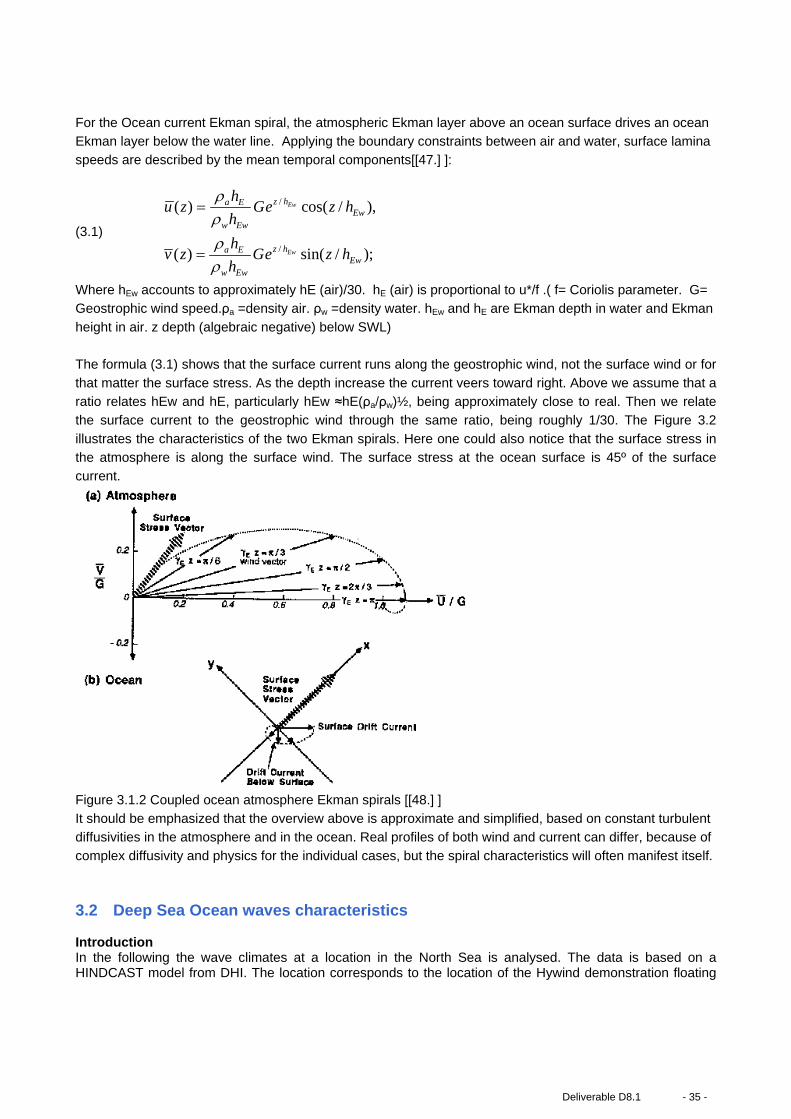
height in air. z depth (algebraic negative) below SWL) The formula (3.1) shows that the surface current runs along the geostrophic wind, not the surface wind or for
that matter the surface stress. As the depth increase the current veers toward right. Above we assume that a ratio relates hEw and hE, particularly hEw ≈hE(ρa/ρw)½, being approximately close to real. Then we relate the surface current to the geostrophic wind through the same ratio, being roughly 1/30. The Figure 3.2
illustrates the characteristics of the two Ekman spirals. Here one could also notice that the surface stress in the atmosphere is along the surface wind. The surface stress at the ocean surface is 45º of the surface current.
Figure 3.1.2 Coupled ocean atmosphere Ekman spirals [[48.] ] It should be emphasized that the overview above is approximate and simplified, based on constant turbulent diffusivities in the atmosphere and in the ocean. Real profiles of both wind and current can differ, because of
complex diffusivity and physics for the individual cases, but the spiral characteristics will often manifest itself. 3.2 Deep Sea Ocean waves characteristics Introduction In the following the wave climates at a location in the North Sea is analysed. The data is based on a HINDCAST model from DHI. The location corresponds to the location of the Hywind demonstration floating
Deliverable D8.1 - 35 -

wind turbine. It is placed 11 km from the Norwegian Shore in a water depth of 220 m as shown in Figure 3.2.11.
Figure 3.2.1 Location of the Hywind demonstration floating wind turbine, where the wave climates are
calculated. As explained, waves in real seas are irregular. In its most simple form a wave realization can be seen as a sum of sinusoidal waves with different amplitude, wave period and phase. The significant wave height, Hs, is the average of the highest one-third of all waves in the wave realization. The mean wave period, Tz, is the mean wave period of all zero down-crossing wave periods and the peak wave period, Tp, is the wave period with the highest energy. For a Pierson–Moskowitz spectrum the relationship between the mean wave period and peak wave period is (3.2.1) 𝑇𝑝 = 1.41𝑇𝑧. To determine the design wave climate often hind cast modelling is used. In the HINDCAST modelling, measured data are used to predict how waves, currents and water levels will be in the future. The HINDCAST modelling is driven by atmospheric pressure and wind from meteorological data. To do proper HINDCAST modelling, information about the bathymetry and tidal level are also necessary. The models are calibrated and validated against measured data. Since the models cover a large area the long-term calibration can be made for areas with available long measurement data. The HINDCAST study are used to establish a data base of environmental data of wind speeds, significant wave height, wave peak periods, maximum wave heights and periods, current velocities and water depths. In the design basis for the fatigue analysis the wave climate for each wind speed is gathered in a Tp-Hs matrix or Tz-Hs matrix, where the probability of occurrence for each combination of the significant wave height and wave period is stated. The wind and wave data are gathered in bins, the bins of the wind speed cover often 2 m/s, the bins of the significant wave height cover 0.5 m and the bins of the peak wave periods 1 s. In case of misalignment between wind and wave directions a fourth dimension is included in the scatter diagrams. All these combinations of wind speed, wave height and wave period cannot be included in the design. A lumping of the wave and wind parameters is therefore carried out to reduce the number of load cases. One method to do the lumping is described in [[43.] ]. Kühn uses that the wave loads on offshore wind turbines on monopile foundations are inertia dominated (depend on the acceleration). For inertia dominated structures the stress range is roughly proportional to the significant wave height and the damage is therefore proportional to Hs. Further Kühn states that the damage is proportional to the number of cycles which roughly can be assumed to be equal to 1/Tz2
1 The figure is from the homepage http://www.4coffshore.com/windfarms/hywind-norway-no04.html 2 Strictly valid for monopole structures-for floating wind turbines this might be different
- 36 - Deliverable D8.1

(3.2.2) 𝐻𝑠 = 𝐻𝑠𝑚𝑃𝐻𝑠
∑ 𝑃𝐻𝑠𝑇𝑧
(3.2.3) 1𝑇𝑧
=∑
𝑃𝑇𝑧𝑇𝑧
∑ 𝑃𝐻𝑠𝑇𝑧.
Here 𝑃𝐻𝑠 and 𝑃𝑇𝑧 is the probability that the given wave height or wave period occurs together with a given wind speed and 𝑃𝐻𝑠𝑇𝑧 is the joint probability of wave height and wave period occurs together with a given wind speed. The equivalent load based on 𝐻𝑠 and 𝑇𝑧 and a given wind speed may not result in the same equivalent load when based on the full scatter diagram and can therefore be adjusted by a scaling factor 𝜈 (3.2.4) 𝐻𝑠,𝑠𝑐𝑎𝑙𝑒𝑑 = 𝜈𝐻𝑠
(3.2.5) 𝑇𝑧,𝑠𝑐𝑎𝑙𝑒𝑑 = 𝑇𝑧𝜈
.
However, this scaling is sometimes disregarded and the fatigue analysis is instead based on the unscaled values. To find the extreme design data, methods such as peak over threshold are most often used. The extreme events are fitted to an extreme value distribution (often Weibull distributions are used), and extrapolated to the probability of occurrence level, which is used in the design. It is important to be careful in the choice of distribution and the data fitting, because the results may be sensitive to for example a change of the threshold value.
The wave period corresponding to the extreme wave height from DNV-OS-J101 [[3.] ]3 is repeated here
(2.3.12) 11.1𝐻𝑠𝑔
≤ 𝑇 ≤ 14.3𝐻𝑠𝑔
.
The wave period inside this region which results in the largest wave force should be used. With these extreme waves it is necessary to use a nonlinear wave theory in order to describe the waves properly. Often
stream function wave theory is used. The wave climate The present wave climates are based on a HINDCAST model from DHI where they used measured wave and wind data from the last 33 years from 1980 to 2013. Based on the hind cast model they have made a scatter diagram with the mean wave period and peak wave periods as function of the significant wave height and each sea states probability of occurrence. Also the wave direction is given as function of the significant wave height and each directions probability of occurrence is stated. Further the extreme wave heights exceedance probabilities are given. In the present analysis the wind is not considered. The data therefore only give the probabilities of occurrence of the significant wave heights. In Figure 3.2.2 the probabilities of occurrence of each sea state are stated. The wave height and wave period are gathered in bins of 1 m and 1 s respectively.
3 As per standard (3.1.6) is valid also for deep sea conditions
Deliverable D8.1 - 37 -

Figure 3.2.2 Probability of occurrence of the significant wave height (Hm0 in figure) and mean wave period (T02 in figure) The probabilities of occurrence of the significant wave heights are also shown in a probability plot in Figure 3.2.3. The mean wave periods occurring for each significant wave height can be lumped by use of equation (3.2.3). The lumping result in one mean wave period for each significant wave height as shown in Figure 3.2.4, where the total Hs - Tz scatter also is shown. The lumped peak wave periods based on the relationship in equation (3.2.1) are also shown in Figure 3.2.4 with blue stars. The relation between Hs and Tp given in equation (2.3.12) are also shown in the figure. It is seen that the predicted Tp values are larger than the maximum limit with α =14.3 despite that the site considered are deep water. In order to describe the relation between Hs and Tp then α has to be around 16 also shown in Figure 3.2.4. This comparison clearly shows that equation 2.3.12 only can be used as a guideline and is not representative for all sites in the North Sea.
Figure 3.2.3 The probabilities of occurrence of the significant wave height.
- 38 - Deliverable D8.1
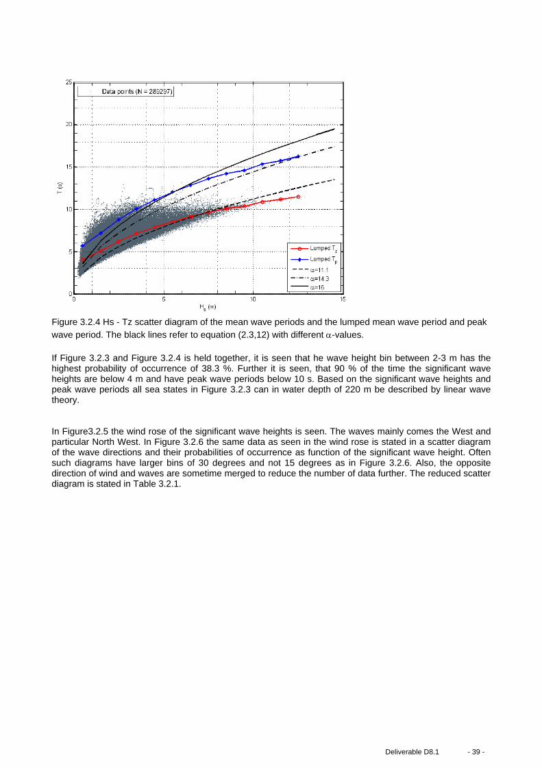
Figure 3.2.4 Hs - Tz scatter diagram of the mean wave periods and the lumped mean wave period and peak wave period. The black lines refer to equation (2.3,12) with different α-values. If Figure 3.2.3 and Figure 3.2.4 is held together, it is seen that he wave height bin between 2-3 m has the highest probability of occurrence of 38.3 %. Further it is seen, that 90 % of the time the significant wave heights are below 4 m and have peak wave periods below 10 s. Based on the significant wave heights and peak wave periods all sea states in Figure 3.2.3 can in water depth of 220 m be described by linear wave theory. In Figure3.2.5 the wind rose of the significant wave heights is seen. The waves mainly comes the West and particular North West. In Figure 3.2.6 the same data as seen in the wind rose is stated in a scatter diagram of the wave directions and their probabilities of occurrence as function of the significant wave height. Often such diagrams have larger bins of 30 degrees and not 15 degrees as in Figure 3.2.6. Also, the opposite direction of wind and waves are sometime merged to reduce the number of data further. The reduced scatter diagram is stated in Table 3.2.1.
Deliverable D8.1 - 39 -

Figure3.2.5 Wind rose of the wave directions and the directions probabilities of occurrence as function of the significant wave height (Hm0 in the figure).
Figure 3.2.6 Scatter diagram of the wave directions and the directions probabilities of occurrence as function of the significant wave height (Hm0 in the figure).
Table 3.2.1 The reduced wave directions and the directions probabilities of occurrence. The bins are 30 degrees and the opposite direction of the waves is merged.
Dir/Hs 0.5 1.5 2.5 3.5 4.5 5.5 6.5 7.5 8.5 9.5 10.5 11.5 12.5 Total
[352.5-22.5] [172.5-202.5[
4.3 9.4 4.2 1.6 0.70 0.35 0.16 0.072 0.027 0.006 0.002 0.001 0.001 20.9
[22.5-52.5] [202.5-232.5[
6.5 7.6 3.4 1.4 0.71 0.37 0.19 0.087 0.038 0.021 0.004 0.001 0.001 20.4
[52.5-82.5[ [232.5-262.5[
3.4 5.3 3.3 1.8 0.84 0.49 0.23 0.090 0.049 0.023 0.007 0 0 15.6
[82.5-112.5[ [262.5-292.5[
2.5 3.6 2.6 1.4 0.63 0.31 0.13 0.054 0.025 0.009 0 0 0 11.4
- 40 - Deliverable D8.1

[112.5-142.5[ [292.5-322.5[
2.6 4.6 3.0 1.5 0.80 0.39 0.16 0.038 0.011 0.002 0.001 0 0 13.1
[142.5-172.5[ [322.5-352.5[
2.96 7.6 4.8 2.1 0.77 0.26 0.076 0.021 0.002 0 0 0 0 18.6
Total 22.3 38.3 21.3 9.9 4.4 2.2 0.95 0.36 0.15 0.06 0.01 0.002 0.002 100
Extreme data For the extreme design load cases the wave heights for different return periods are calculate as shown in Figure 3.2.4. Following equation (2.3.12), the corresponding wave periods should be in the range stated in Figure 3.2.4 If the significant wave height is based on a 3 hours record and the waves are Rayleigh distributed the maximum wave height can be assumed to be according to DNV-OS-J101 [[3.] ] be found from the significant wave height formula: (3.1.6) 𝐻𝑚𝑎𝑥 = 1.86𝐻𝑠. The maximum wave heights are stated in Table 3.2.2. The corresponding maximum wave periods are found from equation (2.3.12) and are stated in Table 3.2.2.
Figure 3.2.7 The extreme significant wave height (Hm0 in figure) for different return periods, TR.
Table 3.2.2 The extreme wave height and wave period for different return periods
TR (year) 1 10 50 100
Hs (m) 8.9 11.4 13.1 13.6
T (s) 10.6-13.6 13.0-15.4 12.8-16.5 13.1-16.8
Hmax (m) 16.6 21.2 24.4 25.3
Tmax (s) 14.4-18.6 16.3-21.0 17.5-22.6 17.8-23.0
Deliverable D8.1 - 41 -

For a 50 year return period the expected largest wave height is 24.4 m and the wave period between 17.5-22.6 s.
Measurements The data have been measured and provided by DHI for this section. Another set of data has kindly been provided by the Norwegian Meteorological Institutte4. Limited measured data based on 1-hour intervals was
available for the site Utsira close to Hywind site, with only a number of limited time periods: August 2009 – May 2010, January 2011 – March 2011, and August 2011 – September 2011. To confidently characterise the site on met-ocean conditions, longer and more homogenous measurement series would be required, and
hence statistical results cannot be presented here on the basis of these short discontinuous measurement periods. For example, wave scatter diagrams generated for the different measurement periods are significantly different from one another, indicating that suitable conditions cannot be selected for the design
of the floating wind turbine based on these data. The same applies for the wind data, where dependable wind speed probability distributions and subsequently joint wind-wave distributions cannot be derived.
However, the deterministic part of the correlation between wave height and wind speed at 10 m height is less influenced by missing data and is therefore analysed for comparison with previous data. The quadratic fit is shown in Figure 3.2.8, together with the function used in Figure 2.4.5.
Figure 3.2.8 Hs versus the 10 meter wind speed for the Demo-site considered with wave measurements. The HS values for the site are fitted with a quadratic fit as shown in the plot. Also the function presented (2.4.1) and used in Figure 2.4.5 is shown for comparison and us.
The two functions presented on Figure 3.2.8 are obviously different in the wind interval with most data. An additional difference is that that Figure 2.4.5 is based on lumped statistics, while the scatterplot in Figure
3.2.8 is based on raw data2.
- 42 - Deliverable D8.1
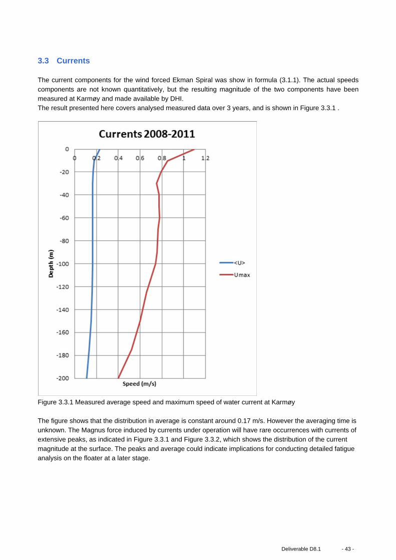
3.3 Currents The current components for the wind forced Ekman Spiral was show in formula (3.1.1). The actual speeds
components are not known quantitatively, but the resulting magnitude of the two components have been measured at Karmøy and made available by DHI. The result presented here covers analysed measured data over 3 years, and is shown in Figure 3.3.1 .
Figure 3.3.1 Measured average speed and maximum speed of water current at Karmøy
The figure shows that the distribution in average is constant around 0.17 m/s. However the averaging time is unknown. The Magnus force induced by currents under operation will have rare occurrences with currents of extensive peaks, as indicated in Figure 3.3.1 and Figure 3.3.2, which shows the distribution of the current
magnitude at the surface. The peaks and average could indicate implications for conducting detailed fatigue analysis on the floater at a later stage.
Deliverable D8.1 - 43 -

Figure 3.3.2 Occurrence of currents at surface To get an indication of the order of magnitudes of the Coriolis action on the water particles, the met-ocean
data from Furewik4 have been analysed for different water depths. The met-ocean data analysed show a variation which depends on whether conditions predominantly consisting at this site close to Western coast of Norway. The analysis of a long time series has to be
analysed in terms of probabilities under a certain conditions, which for this dataset as explained on the basis of limited data would provide false probabilistic results. Instead some typical one-hour sequences of the current at various depths are presented along with the resulting Magnus transverse lift force for the 5MW
DeepWind rotating cylinder considered in a fixed position. The polar plots in Figure 3.3.3 show that over an arbitrary period of 6 hours, the current directions and magnitudes at a number of water depths vary significantly. In particular in some cases the current magnitude
does not monotonically decrease with water depth, with increases in current magnitude between intermediary water depths, which does not follow the mathematical relations set out in eq. 3.1. For example, in the top right polar plot in Figure 3.3.3 the current velocity at 20 metres is around 0.1 m/s whilst at 50
meters and 70 metres the current velocities are 0.22 m/s and 0.17 m/s, respectively. The subsequent impact of these observations is that the Magnus forces experienced by the rotating cylinder will vary temporally in both magnitude and direction along the length of the submerged cylinder that operates through these
laminae of different sea currents. To illustrate this, Figure 3.3.4 to 3.3.6 provide polar plots of the local currents and corresponding generated
Magnus forces at three points along the spar for 3 1-hour periods: 0, 54 and 108 metres depth (corresponding to top, middle and bottom of the spar). For each polar plot, the current is normalised by the maximum value for that time period and the same is done for the Magnus force, thus providing the relative
magnitudes at the different water depths. As is evident from the plots, the predicted Magnus force varies significantly in both magnitude and direction along the length of the cylinder, and in some cases (Figures 3.3.4 and 3.3.6) the Magnus force at the bottom of the cylinder is significantly larger than that at the middle
of the cylinder. Figures 3.3.7 to 3.3.9 present polar plots of the normalised of the mean current and total Magnus force experienced by the whole cylinder for the same 3 1-hour time periods. The figures also illustrate the position of the centroid of the Magnus transverse force along the length of the cylinder. As can
be seen from the latter two figures, the global Magnus transverse force does not necessarily coincide with a direction perpendicular to the mean current direction. Furthermore due to the nonlinear variation of current
- 44 - Deliverable D8.1

magnitudes along the length of the cylinder, the Magnus force centroid is not located at the geometrical centroid of the cylinder and also moves along the length of the cylinder over time.
The implications of these observations are that due to the varying current directions, Magnus force components along the cylinder would partially cancel out each other and/or induce additional inclining moments on the floating cylinder. Subsequently this would have an significantly impact on simulations and
deriving wind turbine structural loads and fatigue; so far steady, unidirectional currents were applied in aeroelastic simulations which would result in significantly different hydrodynamic loads than what is presented here, potentially having an adverse impact on the final structural design and cost of the floating
wind turbine. The emphasis of this section is to demonstrate the importance of including the described current characteristics in numerical simulations to more appropriately predict structural and fatigue loads, leading to a more optimal floating wind turbine design.
Figure 3.3.3 Series of polar plots depicting depth and temporal variation of current with water depth over six hours, from 1400-1900. Measurement from Utsira. The depths are indicated by colour in the 3-100 meter interval.
Deliverable D8.1 - 45 -
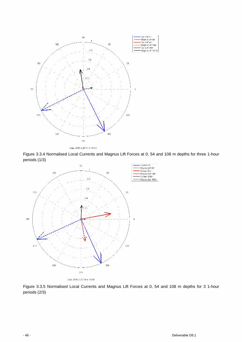
Figure 3.3.4 Normalised Local Currents and Magnus Lift Forces at 0, 54 and 108 m depths for three 1-hour
periods (1/3)
Figure 3.3.5 Normalised Local Currents and Magnus Lift Forces at 0, 54 and 108 m depths for 3 1-hour
periods (2/3)
- 46 - Deliverable D8.1
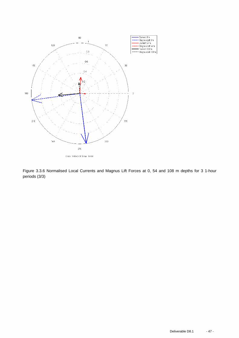
Figure 3.3.6 Normalised Local Currents and Magnus Lift Forces at 0, 54 and 108 m depths for 3 1-hour
periods (3/3)
Deliverable D8.1 - 47 -

Figure 3.3.7 Normalised Mean Currents and Global Magnus Lift Force for 3 1-hour periods, averaged over
the depth (0-108m) of the rotating cylinder (1/3)
Figure 3.3.8 Normalised Mean Currents and Global Magnus Lift Force for 3 1-hour periods(2/3)
- 48 - Deliverable D8.1
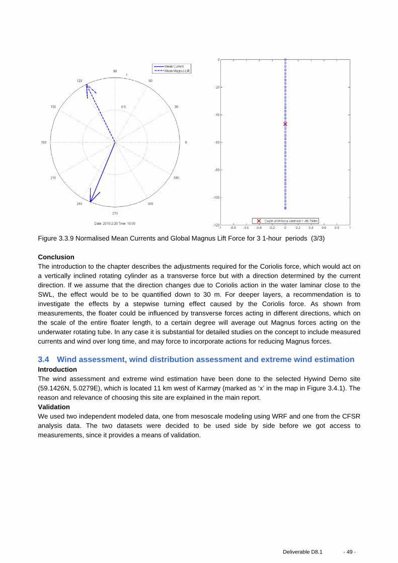
Figure 3.3.9 Normalised Mean Currents and Global Magnus Lift Force for 3 1-hour periods (3/3)
Conclusion The introduction to the chapter describes the adjustments required for the Coriolis force, which would act on a vertically inclined rotating cylinder as a transverse force but with a direction determined by the current direction. If we assume that the direction changes due to Coriolis action in the water laminar close to the
SWL, the effect would be to be quantified down to 30 m. For deeper layers, a recommendation is to investigate the effects by a stepwise turning effect caused by the Coriolis force. As shown from measurements, the floater could be influenced by transverse forces acting in different directions, which on
the scale of the entire floater length, to a certain degree will average out Magnus forces acting on the underwater rotating tube. In any case it is substantial for detailed studies on the concept to include measured currents and wind over long time, and may force to incorporate actions for reducing Magnus forces.
3.4 Wind assessment, wind distribution assessment and extreme wind estimation Introduction The wind assessment and extreme wind estimation have been done to the selected Hywind Demo site (59.1426N, 5.0279E), which is located 11 km west of Karmøy (marked as ‘x’ in the map in Figure 3.4.1). The reason and relevance of choosing this site are explained in the main report.
Validation We used two independent modeled data, one from mesoscale modeling using WRF and one from the CFSR analysis data. The two datasets were decided to be used side by side before we got access to
measurements, since it provides a means of validation.
Deliverable D8.1 - 49 -
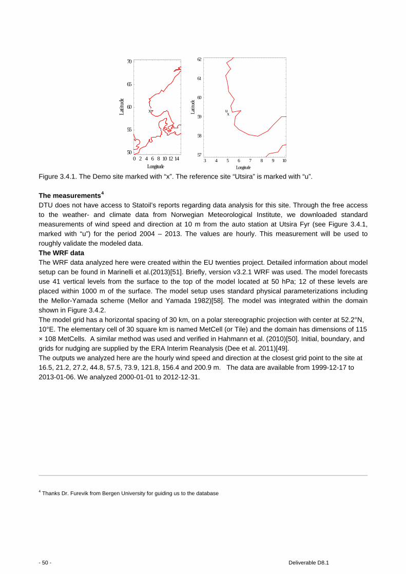
Figure 3.4.1. The Demo site marked with “x”. The reference site “Utsira” is marked with “u”.
The measurements4 DTU does not have access to Statoil’s reports regarding data analysis for this site. Through the free access to the weather- and climate data from Norwegian Meteorological Institute, we downloaded standard measurements of wind speed and direction at 10 m from the auto station at Utsira Fyr (see Figure 3.4.1,
marked with “u”) for the period 2004 – 2013. The values are hourly. This measurement will be used to roughly validate the modeled data.
The WRF data The WRF data analyzed here were created within the EU twenties project. Detailed information about model setup can be found in Marinelli et al.(2013)[51]. Briefly, version v3.2.1 WRF was used. The model forecasts use 41 vertical levels from the surface to the top of the model located at 50 hPa; 12 of these levels are
placed within 1000 m of the surface. The model setup uses standard physical parameterizations including the Mellor-Yamada scheme (Mellor and Yamada 1982)[58]. The model was integrated within the domain shown in Figure 3.4.2.
The model grid has a horizontal spacing of 30 km, on a polar stereographic projection with center at 52.2°N, 10°E. The elementary cell of 30 square km is named MetCell (or Tile) and the domain has dimensions of 115 × 108 MetCells. A similar method was used and verified in Hahmann et al. (2010)[50]. Initial, boundary, and
grids for nudging are supplied by the ERA Interim Reanalysis (Dee et al. 2011)[49]. The outputs we analyzed here are the hourly wind speed and direction at the closest grid point to the site at 16.5, 21.2, 27.2, 44.8, 57.5, 73.9, 121.8, 156.4 and 200.9 m. The data are available from 1999-12-17 to
2013-01-06. We analyzed 2000-01-01 to 2012-12-31.
4 Thanks Dr. Furevik from Bergen University for guiding us to the database
0 2 4 6 8 10 12 1450
55
60
65
70
Longitude
Latit
ude
x
3 4 5 6 7 8 9 1057
58
59
60
61
62
Longitude
Latit
ude
xu
- 50 - Deliverable D8.1
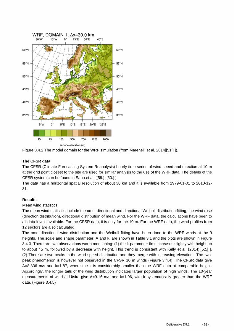
Figure 3.4.2 The model domain for the WRF simulation (from Marenelli et al. 2014[[51.] ]).
The CFSR data The CFSR (Climate Forecasting System Reanalysis) hourly time series of wind speed and direction at 10 m at the grid point closest to the site are used for similar analysis to the use of the WRF data. The details of the CFSR system can be found in Saha et al. [[59.] ,[60.] ]
The data has a horizontal spatial resolution of about 38 km and it is available from 1979-01-01 to 2010-12-31.
Results Mean wind statistics The mean wind statistics include the omni-directional and directional Weibull distribution fitting, the wind rose
(direction distribution), directional distribution of mean wind. For the WRF data, the calculations have been to all data levels available. For the CFSR data, it is only for the 10 m. For the WRF data, the wind profiles from 12 sectors are also calculated.
The omni-directional wind distribution and the Weibull fitting have been done to the WRF winds at the 9 heights. The scale and shape parameter, A and k, are shown in Table 3.1 and the plots are shown in Figure 3.4.3. There are two observations worth mentioning: (1) the k-parameter first increases slightly with height up
to about 45 m, followed by a decrease with height. This trend is consistent with Kelly et al. (2014)[[52.] ]. (2) There are two peaks in the wind speed distribution and they merge with increasing elevation. The two-peak phenomenon is however not observed in the CFSR 10 m winds (Figure 3.4.4). The CFSR data give
A=8.836 m/s and k=1.87, where the k is considerably smaller than the WRF data at comparable height. Accordingly, the longer tails of the wind distribution indicates larger population of high winds. The 10-year measurements of wind at Utsira give A=9.16 m/s and k=1.96, with k systematically greater than the WRF
data. (Figure 3.4.5)
Deliverable D8.1 - 51 -
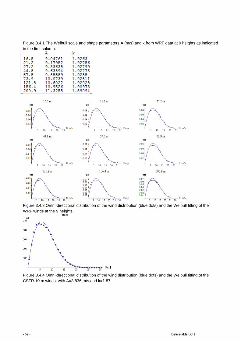
Figure 3.4.1 The Weibull scale and shape parameters A (m/s) and k from WRF data at 9 heights as indicated in the first column.
Figure 3.4.3 Omni-directional distribution of the wind distribution (blue dots) and the Weibull fitting of the WRF winds at the 9 heights.
Figure 3.4.4 Omni-directional distribution of the wind distribution (blue dots) and the Weibull fitting of the CSFR 10 m winds, with A=8.836 m/s and k=1.87
5 10 15 20 25 30Ums0.02
0.04
0.06
0.08
0.10pdf
10 m
- 52 - Deliverable D8.1

Figure3.4.5. Omni-directional distribution of the wind distribution (blue dots) at Utsira and the Weibull fitting
of the measured 10 m winds, with A=9.16 m/s and k=1.96. The WRF and CFSR data have shown good agreement in the wind direction distribution, both showing
dominant winds from the south and north sectors (Figure 3.4.6). Good agreement is also observed for the directional distribution for the mean wind speed, A and k parameters. In general, the distributions of these parameters are in agreement with that of the measurements from Utsira.
Figure 3.4.6. Wind direction distribution in 12 sectors. The black-gray lines are the WRF data (black at 16.7 m and gray at high level, grayer at higher level). The blue curve is the CFSR data. The red curve is the
measurements from Utsira.
5 10 15 20 25 30Ums0.02
0.04
0.06
0.08
pdfOBS 10 m
0 50 100 150 200 250 3000
5
10
15
20
dirsector
perc
enta
ge
all levels
Deliverable D8.1 - 53 -
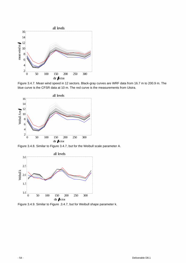
Figure 3.4.7. Mean wind speed in 12 sectors. Black-gray curves are WRF data from 16.7 m to 200.9 m. The blue curve is the CFSR data at 10 m. The red curve is the measurements from Utsira.
Figure 3.4.8. Similar to Figure 3.4.7, but for the Weibull scale parameter A.
Figure 3.4.9. Similar to Figure .3.4.7, but for Weibull shape parameter k.
0 50 100 150 200 250 3002
4
6
8
10
12
14
16
dirsector
mea
nw
ind
ms
all levels
0 50 100 150 200 250 3002
4
6
8
10
12
14
16
dirsector
Wei
bull
Ams
all levels
0 50 100 150 200 250 3001.0
1.5
2.0
2.5
3.0
dirsector
Weib
ullk
all levels
- 54 - Deliverable D8.1

Figure3.4.10. Vertical wind profiles from 12 sectors (sector 1 from north), WRF data (blue dots) and fitting (blue curves).
The wind profiles from 12 sectors have been calculated using the WRF data. This is expected to be useful for the calculation of shear at given heights. But, the calculation of shear is recommended to be done with guidance of measurements.
Veering The WRF data suggest a slight turning of wind (mean direction) to the right of about 3 degrees from the surface to 200 m and the median wind corresponds to a veering of about 5 degrees from surface to 200 m.
This can however not be validated for this site. Offshore lidar measurements from Horn Sea site in the North Sea (at about 59.79N and 5W) have shown a veering of 6 degrees from 75 m to 235 m (Larsén 2013a)[54]. The geostrophic wind direction deviates from the surface wind direction by φ, following approximately:
−= −
1
10
*
1
)ln(
tan180
B
Afzu
πφ ,
Where A1 and B1 are the geostrophic drag law coefficients, u* is the friction velocity and z0 is the roughness length.
Deliverable D8.1 - 55 -

Figure 3.4.11. Vertical distribution of mean wind direction up to 200 m (left) and median wind direction (right), data are from the WRF simulation.
Extreme wind estimation The 50-year return wind has been calculated from the 13-year record of the WRF data as described in section 2.2, from the 32-year CFSR data and from 9-year measurements at Utsira (there are too much
missing data from 2004). We used the Periodic Maximum Method (PMM) in obtaining the 50-year wind (Larsén et al. 2014)[57]. The smoothing effect caused by numerical modeling as discussed in Larsén et al. (2012)[53] is also
observed here for both the WRF and CFSR data. Figure 3.4.12 shows the power spectrum from the WRF wind time series at 16.7 m (red dots) and the spectrum from the CFSR 10 m winds (green curve). The smoothing effect is shown as the tapered out spectrum for f > 1 day-1, as compared to the expected energy
level (the blue line). The spectral correction method as developed in Larsén et al. (2012)[53] is applied to the calculation of the 50-year winds using the two modeled datasets, in which a “corrected spectrum” – the blue curve in Figure 3.4.12 which is a combination of the spectrum from the modeled data for f < 1 day-1 and a
spectral model S(f)=a f-5/3 for f > 1 day-1 is used to obtain the zero and second order spectral moments when calculating the peak factor. An equivalent 1 hour value is obtained when the spectral correction is done to a resolution of 12 day-1 , and an equivalent 10 min value is obtained when the correction is done to 72 day-1.
Figure 3.4.12. The power spectrum from WRF wind at 16.7 m (red), CFSR winds at 10 m (green) and a spectral model S(f)=a f-5/3 for f>1 day-1(blue) and measurements from Utsira (black).
In order to make direct comparison with the measurements, the hourly 50-year wind at 10 m were calculated. Using PMM with a basis period of 6 months, the measurements from Utsira give the hourly 50-year wind at
204 206 208 210 2120
50
100
150
200
meandirdeg
heig
htm
186 188 190 192 194 196 198 2000
50
100
150
200
mediandirdeghe
ightm
0.001 0.01 0.1 1 10
0.01
1
100
f 1day
Sf
- 56 - Deliverable D8.1

10 m of 36 ± 9 m/s (Figure3.4.13). Using the spectral correction method, the 10 min 50-year wind at 10 m is obtained as 40 m/s. This corresponds to 10 min 50-year wind at 100 m of 51 m/s using the roughness length as described in Donelan et al. (2004)[76] with an assumption of a logarithmic wind profile.
In Table 2, the 50-year wind at 100 m and 10 m are calculated at a temporal resolution of 1 h and 10 min, using four different datasets and four different methods, denoted as a, b, c and d. Data-a corresponds to the WRF data as described in section 2.2. Data-b corresponds to the CFSR data described in section 2.3. Data-
c corresponds to the storm simulation made in Larsén (2013b)[55] and Data-d are measurements from Utsira. Obviously, all modeled data underestimate the extreme wind estimation; given the measurements from
Utsira can represent the extreme wind at the Demo site. This is of course related to the challenges in storm modeling in coastal areas. Regarding the data in Larsén et al 2013a.[54] this Demo site seems too close to their model boundary where the uncertainty is expected
to be large.
Figure 3.4.13. T-year return wind distribution from 10 -m measurements from Utsira. The basis period of 6 months was used, so that 100 on the x-axis corresponds to 50-year.
Discussion The estimates in this report can only be treated as reference before data validation takes place.
For the wind resource assessment, the independence data sources, WRF climate runs from the TWENTIES project and the CFSR data have shown some consistent statistics while there are also some discrepancies. The 50-year wind has been obtained here using the WRF climate modelling output, as well as from a
commercial project Larsén 2013b[[55.] ]. There is a quite large difference between the estimates from the three methods.
0.5 1.0 5.0 10.0 50.0 100.010
15
20
25
30
35
40
2 times Return Years
U Tms1
Deliverable D8.1 - 57 -

Table 3.4.1 The 50-year wind at 100 m and 10 m from four data sets with different methods for the Demo site.
DATA a. WRF climate (1h, 30 km)
2000 – 2012
b. CFSR (1h, 38 km)
1979 – 2010
c. WRF storm episodes (10min, 5
km)
1999 – 2012
d. OBS from Utsira (1 hour)
2005 – 2013
U50 at 100 m
(m/s)
1h 32.8 39.0 37.4 46
10min 36.5 44.0 39.1 51
U50 at 10 m 1h 31 29 36
10min 35 31 40
U50 at 16 m 1h 28 36
31
Possible uncertainties sources
Too coarse resolution
for a coastal site.
The distribution of max
wind and mean as
produced from the
model does not follow
Gaussian.
No coupling of wind
and waves
Too coarse resolution for a coastal site.
The Demo site is too close to the model domain
boundary. The dynamics of
wind and wave need to be coupled in the
modeling.
Too short time series.
A bit away from the Demo site – which might matter
because it is the coastal site.
3.5 Comparison between the parameters in section 2.4 and from the project site in
section 3.4. As expected both the wind and the wave direction at the demo site are influenced by the nearness of the Norwegian coast.
However, the wind distributions of Figures 3.4.3-3.4.5 and section 2.4 are within the same envelope, see Table 2.4.1. As discussed in section 3.4 the methods for assessing the 50 year wind are uncertain for all the methods and data applied. However, it is worth noting that the 10 meter V50 from Table 2.4.1, ranges in the
interval 31-39 m/s, which is largely the same interval coming out in Table 3.4.2. The Hs and Tp values in Table 3.2.2 for Hs and Tp for 50 years and 1 year are significantly larger at the demo-site than from the sites in section 2.4. Additionally, the scatter gram in Figure 3.2.4 for Tp versus Hs is show a
relation that is largely outside the interval for similar curves in Figure 2.4.6. Indeed it is outside the standard interval, given in (2.3.12). The relation between Hs and V10 depicted in Figure 2.4.5 is compared to the scatter plot obtained from
somewhat insufficiently homogeneous measurements at Utsira, and shown in Figure 3.2.8. As seen the Utsira data are significantly above the data from section 2.4. Comparing the extreme wave heights, HS1 and HS50, for 1 year and 50 years, from Table 2.4.1 and Table
3.2.2, we see that they are both significantly larger at the DeepWind demo-site, than found for the sites in section 2.4. In summary, we conclude that the wind conditions at found in section 2.4 and at the demo-site are quite
similar as far as can be judged from the respective analyses. The wave climate on the other hand seems
- 58 - Deliverable D8.1

more severe at the DeepWind site, especially with respect to more extreme events, which is probably to be expected, given the greater water depth and the large fetch possibilities for this site.
4. SCALING OF WIND AND WAVE CONDITIONS FOR PHYSICAL MODEL TEST
In this section, following [[46.] ] we review the relevant scaling considerations for offshore wind turbines that
are subject to simultaneous loads from waves and wind. A recent study for a floating wind turbine is reviewed too. Next, the suggested scaling methodology is derived and a scaling method for structural parameters and wind/wave climate parameters are devised. The scaling method is applied to a simple
numerical model for a floating TLP (Tension Leg Platform) wind turbine, subjected to an external climate of section 2.4. It is demonstrated that a perfect reproduction of structural response at model scale can be achieved, provided that the structural loads are reproduced correctly. This requirement implies a re-design of
the blades due to the smaller Reynolds number at model scale and assumes insensitivity of the hydrodynamic load coefficients to the hydrodynamic Reynolds number. The limitations of the scaling procedure are discussed. In section 4.6 elements to a similar testing of the DeepWind demonstrator is
presented and discussed. 4.1 Review of existing scaling studies and relevant non-dimensional numbers Although offshore wind turbines are predominantly bottom fixed, most of the existing studies of simultaneous wind and wave loads in offshore wind energy are concerned with floating wind turbines. This is attributed to the larger response of the support structure compared to bottom fixed structures.
Until now, only little material has been published regarding FOWT (Floating Offshore Wind Turbine) scale model testing. The scale testing efforts related to prototypes of FOWT (e.g. Statoil’s Hywind prototype or EDP’s WindFloat) have not been published. The most comprehensive published FOWT scale test was
performed in the United States by collaboration between the National Renewable Energy Laboratory, NREL, and the University of Maine, UMaine. Experiences from this test are reviewed in the following. Further, a review of relevant scaling laws and a list of relevant publications addressing this issue are provided.
The FOWT study on DeepWind demonstrator was carried out partly under test conditions in the fjord at DTU campus Risø, and in the ocean laboratory of MARIN(NL). The rotor diameter is 2 meter, and the overall
length of the tube is 5 m. 4.1.1 List of Symbols for the review cs = speed of sound C = wave celerity Fr = Froude number
g = acceleration of gravity l = characteristic length KC = Keulegan-Carpenter number
Ma = Mach number Ω = rotor angular velocity [radians/sec] ρ = fluid density
R = blade radius Re = Reynolds number
Deliverable D8.1 - 59 -

St = Strouhal number TSR = tip speed ratio μ = fluid dynamic viscosity
U = free stream fluid velocity 4.1.2 Important Non-Dimensional Numbers Non-dimensional numbers are dimensionless fractions or products resulting from relations between parameters defined by the fundamental quantities L, M, and T (length, mass, and time, respectively). The two most important non-dimensional numbers to conserve when modelling a scaled rotor system are the
Lock Number and the Reynolds Number [27,28]. These reflect the most important parameters involved with aerodynamic and elastic forces. The Froude Number is the most important non dimensional number to preserve when modelling floating structures for hydrodynamic similarity [29,30].
Geometric Scaling Factor (λ) The geometric scaling factor describes the ratio of the physical length between the full scale turbine and the
scaled test model. The value of λ is constrained by the size of the testing facility, feasibility of model construction, scaling law similitude requirements, and the project’s budget.
Froude Number (Fr) The Froude number is a dimensionless number that defines the ratio of inertial forces to gravitational forces in a fluid. When a free surface wave propagates within a fluid, the Froude number can be defined in the
following way [29]: (4.1.1) Frwave= C/(gl)½
In wind-wave basin model tests, the Froude number is the most frequently conserved dimensionless number
to ensure hydrodynamic similitude. While viscous effects do affect FOWT platform hydrodynamics, they are considered small in comparison to inertial effects at both test and model scales. Viscous effects are mostly manifested in the thin boundary layer around floating bodies [31].
Reynolds Number (Re) The Reynolds number is defined as the ratio of inertial forces to viscous forces in a flow. For a cylinder
exposed to a fluid with velocity u, the Reynolds number is
(4.1.2) Re=ρDU/μ
The Reynolds number is important in fluid systems because qualitatively, flow over a body acts similarly for
identical Reynolds numbers. Hereby e.g. lift and drag coefficients can be paramterized in terms of the Reynolds number [33]. Because of the small length scales at which models are tested, there is almost always Reynolds number mismatch between model and full scales that cannot be resolved unless there is a
change in the fluid of the system (i.e. viscosity or density) [27,32]. Although this has been done successfully in the helicopter industry, we believe it is out of the scope of existing wind-wave basin test facilities. This mismatch is often combated by using airfoils that have coefficients of lift and drag with minimal dependence
on Reynolds number. This is especially important in the low Reynolds number regimes encountered in model testing [27].
- 60 - Deliverable D8.1

Keuligan-Carpenter number (KC) The Keuligan-Carpenter number is a characteristic number for planar oscillatory flows defined as
(4.1.3) KC=Um Tw / D, where Um is the maximum velocity in the outer flow, Tw is the period of the flow and D is the cylinder
diameter. It provides a measure for the length of a horizontal particle path in the outer flow relative to the cylinder diameter. For small KC numbers, there will be no flow separation around the cylinder, where for large KC numbers, vortex shedding will occur during the flow cycle. As a rule of thumb, the balance between
inertia and viscous forces is equal to 20/KC [15]. Small KC numbers thus implies dominant inertial loading, while large KC numbers are associated with dominant viscous loading.
Tip Speed Ratio (TSR) The tip speed ratio is the ratio of the rotor’s velocity to the wind’s free stream velocity:
(4.1.4) TSR=ΩR/U Maintaining a constant TSR is one of the most basic procedures used to preserve similarity in scaling a wind
turbine system [34]. If the TSR and the geometry of the blades are scaled similarly, the flow geometry over the blades will be preserved. This statement is only an approximation because the Reynolds number will vary as the scale of the blade changes, therefore causing flow dissimilarity. However, TSR consistency
should still be realized in model testing, and is compatible with Froude similitude when used to constrain rotational frequencies and wind speed [29].
Mach Number (Ma) The Mach number is the ratio of the flow velocity to the speed of sound, and is an influential parameter in gas dynamics [35] :
(4.1.5) Ma=U/cs
The conservation of the Mach number is often employed in aerodynamic model scaling because it characterizes compressibility effects [30]. At Mach numbers below 0.3, flow can be considered incompressible [35]. Figure 3.1.1 depicts the Mach number for a full size and model size (1:45) NREL 5 MW
reference rotor. It is seen that compressibility effects can be ignored at both scales because the Mach number remains below 0.3. This means that conserving the Mach number’s exact value between scales is not necessary for aerodynamic similitude [29].
Deliverable D8.1 - 61 -

Figure 3.1.1. Mach number calculation for a full scale NREL 5 MW reference turbine and its 1/45th scale model (calculated using BEM theory) [29]. The Mach numbers in both systems are below 0.3, which validates the assumption of incompressible flow at full and model scales. This data was generated in a
simulation where the wind speed was 11.4 m/s and the rotor TSR was 6.958.
Strouhal Number (St) The Strouhal number is the dimensionless vortex shedding frequency for a body emerged in a viscous fluid (4.1.6) St=f D / V
If Froude scaling is employed, the Strouhal number cannot always be maintained because of its dependence on the Reynolds number. However, the Strouhal number stays at a value of 0.2 for a range of Reynolds
number and its effects have been neglected in past experiments [29]. The Strouhal number is typically conserved to ensure similitude in vortex induced vibration (VIV) driven effects, which may not be important for FOWT (specifically TLP) model testing.
4.1.3 Dominant scaling methodologies for FOWT
Geometric Scaling The simplest method of creating a scale model is to scale the full turbine’s geometry by a factor of λ, thereby creating a miniature turbine that preserves all relative length dimensions. However, the performance of turbines at different length scales depends on more than their geometry and crucial dissimilarities will exist if
this is the only scaling method chosen. For instance, every non-dimensional number (except λ) in the previous section depends on environmental parameters independent of the model’s geometry, meaning that the dynamic and kinematic effects described by such non-dimensional numbers will differ between the model
and full scale turbines unless efforts are made to equate the values of these numbers at all scales.
- 62 - Deliverable D8.1

Dynamic and Elastic Scaling In order for model size turbines to act dynamically similar to full size turbines, one must ensure that the model’s aerodynamics and hydrodynamics match those of the full scale system [31]. Additionally, dynamic
similarity requires that natural frequencies and gyroscopic moments are properly scaled from the full to model scale [36]. It has been well established by the oil and gas industry that Froude number equality between the model scale and full scale is most effective in achieving hydrodynamic similarity. Froude scaling
has been succesfully applied in several model studies of floating wind turbines including those of NREL and UMAINE.
Froude scaling has further been validated by NREL FAST simulations [36]. However, these tests assume that Reynolds number dependent aerodynamic parameters (airfoil Cl, Cd, and viscous damping) were kept constant between model and full scales, an assumption that is difficult to realize in physical modelling. In
addition to Froude scaling, the TSR should be held constant at different scales in order to yield consistency in FOWT kinematics and flow geometries. This will be further detailed in this report.
The scaling methodology proposed in this report is the dynamic and elastic scaling, based on preservation of the Froude number and tip speed ratio. This will be detailed in section 4.2. 4.1.4 UMAINE scaled FOWT testing review The University of Maine designed their tower to mimic the dynamic behaviour of the OC3 Hywind tower by scaling the lowest frequency modes and center of gravity according to Froude similarity [29]. The mass of the
tower failed to directly follow Froude scaling, because a mass-scaled tower construction was impractical and difficult in initial designs. UMaine justified and compensated for this dissimilarity by scaling the combined mass of the tower, nacelle, and rotor. The nacelle was overweight, and the lightweight tower would help
compensate. The tower had a fore aft fundamental bending frequency that was only 5.4% lower than desired and the center of gravity for the model was 3.3% higher than desired [29]. The model tower diameter was 3.7 times smaller than a Froude scaled diameter, and UMaine considered this to be advantageous because it
decreased aerodynamic interaction between the tower and the turbine, something the available NREL software could not simulate [37,29].
University of Maine’s goal when designing blades was to keep them lightweight and to have the airfoil cross sections to remain as consistent as possible with the full scale model. Priority was given to gathering information about the global responses of the FOWT system, not the “blade deformation, rotor dynamics,
and higher order aero-elastic effects” [29]. Geometric redesign was also avoided. Blades were constructed out of carbon fiber to eliminate as much
blade flexibility as possible and reduce the number of variables in testing. This made blade tip deflections negligible and limited the chances of blade failure during experiments. The low weight of carbon fiber was advantageous because of the small blade mass required for Froude consistency in rotor mass and
gyroscopic moments. A mold and bladder process was used to fabricate 15 blades with a mass of 0.130 kg. This was .010 kg
lower than Froude scaled mass, which benefited UMaine by making up for the overweight nacelle and testing wires [29].
The blade deflections were only 2% of theoretical maximum blade deflections, which satisfied UMaine because of the blade’s near-rigid nature. The rotor was unable to produce Froude scaled thrust when the
Deliverable D8.1 - 63 -

testing wind speed was constrained by the wind speed to wave celerity ratio (α), so tests were run in faster winds. Doing so eliminated the possibility of testing at TSR’s higher than five, because the rotor had not been designed for such high angular velocities [36].
Besides the scaling issues described above, UMAINE used a cable to collect the data from the FOWT, that might have influenced the floater motions during the test. Therefore it is recommended, that a lightweight
cable or a wireless data acquisition system is used in future tests. 4.2 Recommended scaling method The proposed scaling method is derived in this section. It is consistent with the one desribed by Martin [29]
apart from the inclusion of a different water density at prototype scale and model scale in the present scaling. Such a difference will often occur due to the use of fresh water in model tests, opposed to the sea water at prototype scale.
For model tests with combined wind and wave forcing, the main interest is the global motion of the structure subject to the aero- and hydro-dynamic loads plus the loads from mooring and gravity. The ratio of these
loads must therefore be preserved between prototype scale and model scale. Further, as the loads are dynamic in time, the frequencies of the loads, the structural frequencies and the rotor frequency must scale consistently. These requirements define the scaling of all relevant quantities and are derived in the following.
The scaling can be applied to e.g. model tests of floating wind turbines, as illustrated in Figure 3.2.1. The proposed scaling preserves the Froude number and KC number for the hydrodynamic motion and the tip speed ratio for the rotor. The Reynolds number for water and air, however, are not preserved. This leads to
the requirement of a re-design of the blades to achieve the correct thrust force. Further, the invariance of the hydrodynamic force coefficients (inertia and drag coefficients) to the hydrodynamic Reynolds number should be checked and significant differences be compensated, see e.g. [44]. Also, but of less practical impact, the
Weber number for water (surface tension) and Mach number for air (compressibility) are not preserved. It should also be noted that while the proposed scaling leads to a consistent thrust force from the rotor, the
re-designed blades at the model scale Reynolds number might not reproduce a consistent rotor torque. This will lead to an inconsistent power production and an inconsistent dynamic generator moment. The latter moment contributes to the roll-forcing of the platform. Hence, to avoid this imperfection, a reproduction of the
aerodynamic torque of the re-designed blades should be pursued. Most important, as already mentioned, however, is a correct thrust-reproduction. 4.2.1 Scaling of geometric length and mass properties The geometric length scale ratio is defined by
(4.2.1) For a correct dynamic scaling the ratio of structural mass and displaced water mass must be preserved:
(4.2.2)
As the volume scales like λ3 this yields
- 64 - Deliverable D8.1

(4.2.3)
Figure 3.2.1: A floating wind turbine in a wave flume with open jet wind tunnel at DTU (Hansen & Laugesen
[38]). The sketch to the right shows the forces involved. The circled quantities are dimensionless numbers that characterises the environment and the motion.
This defines the scaling of the mass moment of inertia J
(4.2.4)
and the scaling of the area moment of inertia for a structural cross section I
(4.2.5) 4.2.2 Froude scaling of hydrodynamic forces A correct dynamic scaling requires that the ratio of inertial force to gravitational force is preserved
(4.2.6)
Deliverable D8.1 - 65 -

Further, the travelled distance of a water particle over a given time must scale with the geometric length:
(4.2.7)
which defines the global time scale. This constitutes the classical Froude scaling of the hydrodynamic forces and motion. 4.2.3 Aerodynamic scaling For dynamic similarity, the ratio of the aerodynamic thrust force to the gravity force on the structure must be preserved
(4.2.8)
It is desirable that the relative velocity between the structure and air is preserved. Therefore the air velocities must scale like λ1/2. It is therefore necessary to scale the CT values with the density ratio to obtain. (4.2.8)
Hereby, however, the proposed scaling will not preserve the Reynolds number in the air or water. For this
reason a re-design of the blades will be needed to obtain the desired value of CTm. The chosen scaling, however, preserves the tip speed ratio (TSR)
(4.2.9)
as the rotor frequency scales inversely with time Ωp /Ωm = λ−1/2. 4.2.4 Scaling of structural stiffness The structural stiffness must be scaled such that the natural frequencies scale consistently with time. Further the structural deflection must scale directly with the length scale. The appropriate scaling can be derived
from the dynamic beam equation
(4.2.10) Here ρsA is the structural mass per length, x transverse deflection, z the spatial coordinate along the beam
axis, E Young’s modulus, I area moment of inertia and p the transverse load per unit length. It is observed that the first term on the left hand side and the transverse load term scale like (ρwp/ρwm)λ2 while the middle term scales like Eλ. A consistent scaling of the equation of motion is therefore obtained for
- 66 - Deliverable D8.1

(4.2.11)
4.2.5 Check of natural frequency and gyroscopic force The above derivation defines the necessary scaling. A check on the natural frequency and gyroscopic force
is provided. The natural frequency of a cantilever beam of length L is given by
(4.2.12)
Application of the above scaling yields
(4.2.12)
which is consistent with the time scaling t~ λ1/2. The gyroscopic moment from the change of the orientation of the rotor is
where is ω is the rotational vector and J is the mass moment of inertia. The gyroscopic moments scales according to
(4.2.13)
which is consistent with the scaling of force times length. 4.2.6 Properties that may not scale consistently It has already been mentioned that certain properties will not scale consistently with the proposed scaling. These are
1. the aero- and hydro-dynamic Reynolds numbers. 2. the hydrodynamic Weber number 3. the aerodynamic Strouhal number 4. the aerodynamic Mach number 5. the aerodynamic torque 6. the aerodynamic power 7. the generator torque and its contribution to roll-forcing
While (1) is compensated by a re-design of the blades and a check of the hydrodynamic drag and inertia
coefficients, (2-6) are considered of small significance for the global planar motion of the wind turbine. The scaling thus ensures a consistent in-plane motion of the floating wind turbine. For the out-of-plane motion (sway, roll, yaw) the gyroscopic moments will scale correctly, while the roll-forcing from a dynamic generator
torque (7) will not necessarily scale correctly. A correction of this effect is open for future research.
Deliverable D8.1 - 67 -
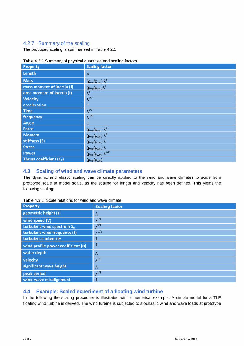
4.2.7 Summary of the scaling The proposed scaling is summarised in Table 4.2.1
Table 4.2.1 Summary of physical quantities and scaling factors Property Scaling factor Length Λ
Mass (ρwp/ρwm) λ3
mass moment of inertia (J) (ρwp/ρwm)λ5
area moment of inertia (I) λ4
Velocity λ1/2
acceleration 1 Time λ1/2
frequency λ-1/2
Angle 1 Force (ρwp/ρwm) λ3
Moment (ρwp/ρwm) λ4
stiffness (E) (ρwp/ρwm) λ Stress (ρwp/ρwm) λ Power (ρwp/ρwm) λ7/2
Thrust coefficient (CT) (ρwp/ρwm)
4.3 Scaling of wind and wave climate parameters The dynamic and elastic scaling can be directly applied to the wind and wave climates to scale from prototype scale to model scale, as the scaling for length and velocity has been defined. This yields the following scaling:
Table 4.3.1 Scale relations for wind and wave climate. Property Scaling factor
geometric height (z) Λ
wind speed (V) λ1/2
turbulent wind spectrum Sw λ3/2
turbulent wind frequency (f) λ-1/2
turbulence intensity 1
wind profile power coefficient (α) 1
water depth Λ
velocity λ1/2 significant wave height Λ
peak period λ1/2
wind-wave misalignment 1 4.4 Example: Scaled experiment of a floating wind turbine In the following the scaling procedure is illustrated with a numerical example. A simple model for a TLP
floating wind turbine is derived. The wind turbine is subjected to stochastic wind and wave loads at prototype
- 68 - Deliverable D8.1

scale. Next, the wind climate, wave climate and wind turbine are scaled to scale 1:50 and the small-scale response is computed in the numerical model. The prototype-scale and small scale responses moment are compared. It is demonstrated that a perfect scaling can be achieved if the aerodynamic thrust and
hydrodynamic loads are reproduced correctly at model scale. Imperfections due to incomplete aerodynamic scaling are discussed. 4.4.1 The TLP wind turbine The wind turbine is the NREL 5 MW reference turbine (Jonkman et al [39]) placed on the NREL-MIT TLP platform (Matha [40]). A sketch of the structure is shown in Figure 3.4.1. The purpose of the example is to
illustrate the scaling in a simplified setting that includes hydrodynamic forces from a wave climate, aerodynamic forces from a wind climate, gravitational forces and structural elasticity. Only two degrees of freedom are retained and several simplifying assumptions are made. These are listed below
• only two degrees of freedom are considered: platform surge and tower flexibility • the tower is considered mass-less and with uniform stiffness. The original tower mass is distributed
onto the top mass and the floater mass. • small deflections for the platform is assumed • the tethers are assumed mass-less and stiff • the rotor mass, nacelle mass are considered as a point mass, placed on top of the tower. Half of the
original tower mass is included. • the floater is considered slender (D/L<0.2) • the waves are considered small to allow application of linear wave theory • spatially coherent turbulence is assumed
Figure 3.4.1. Model sketch for simple model of a TLP wind turbine.
Deliverable D8.1 - 69 -

The structural parameters are listed in Table 4.4.1. Table 4.4.1 Parameters for floating wind turbine at full scale and model scale. Property Symbol Value prototype scale Scaling Value, model scale
(1:50) Floater mass m1 8.774x10⁶ kg (ρwp/ρwm) λ3 68.48 kg Top mass m2 518.5x10³ kg (ρwp/ρwm) λ3 4.047 kg Tower stiffness EI 300x109 Pa (ρwp/ρwm) λ5 936.6 Pa Hub height HH 90m Λ 1.80 m Floater diameter Df 18m Λ 0.36 m Floater draft df 47.89m Λ 0.958 m Water depth h 200m Λ 4.00 m Tether length LT 152.11m Λ 3.04 m Rotor diameter DR 126m λ2 2.52 m Density of air ρa
1.29 kg/m3 1 1.29 kg/m3
Density of water ρw 1025 kg/m3 ρwp/ρwm 1000 kg/m3
4.4.2 Equations of motion The equations of motion consist of Newton’s second law for the floater and the top mass. The displacement of the masses relatively to an earth-fixed reference point is denoted x1 and x2, respectively, as shown in
Figure 3.4.1. The restoring force from the mooring system can be derived by calculation of the excess buoyancy force FBE
(4.4.1) which constitutes the vertical component of the total tether force T. Next, the force triangle for the tether
force, excess buoyancy force and horizontal tether force Fx gives
(4.4.2) where θ is the tether angle with vertical, measured positive in the counter-clockwise direction. Under the
assumption of small deflection angles, this is approximated by -x1/LT whereby
(4.4.3) The elastic bending of the tower constitutes the connection force between the tower and floater, tower and
top mass, respectively. The tower is considered mass-less and no dynamic loads are thus associated with the tower. From standard Euler-Bernoulli beam theory, the force needed to displace the end point of a cantilever beam by a distance x is F=3 EI x/L3, where EI is the stiffness and L is the length. The equations of
motion can thereby be expressed as (4.4.4a)
(4.4.4b)
- 70 - Deliverable D8.1
where FH is the hydrodynamic excitation force, A11 is the hydrodynamic added mass for the floater (derived in next paragraph) and FW is the aerodynamic thrust force from the wind. 4.4.3 Hydrodynamic force The hydrodynamic loading is derived from simple linear wave theory under the assumption of small wave
steepness. The free surface elevation η is expressed as a Fourier series
(4.4.5)
where the amplitudes ap are related to the wave spectrum by
(4.4.6)
and the radian frequency ωp and wave number kp are related through the dispersion relation
(4.4.7)
and further ξp is a set of random phases, uniformly distributed on the interval [0;2]π.
The horizontal fluid velocities are given by
(4.4.8)
and allows computation of the hydrodynamic force on a horizontal cross-section of height dz through the
Morison equation [45] under the assumption of small floater diameter to wave length:
(4.4.9) Here Cm is the hydrodynamic added mass coefficient, CD is the drag coefficient and Af is the cross-sectional
area of the floater. Still under the approximation of linear wave theory, the hydrodynamic forcing is integrated from the bottom of the floater to the still water level. Further, the contribution from x1,tt is moved to the left hand side where it forms the A11 term of the mass matrix:
(4.4.10)
(4.4.11)
Deliverable D8.1 - 71 -

The hydrodynamic coefficients are chosen based on the Reynolds number and KC number to be CD=0.7 and Cm=0.8. 4.4.4 Aerodynamic force The wind force is based on a time series of horizontal wind velocity at hub height
(4.4.12)
where Vhub is the mean wind speed at the hub and the Fourier amplitudes are based on the wind spectrum Sf
(4.4.13)
and further εm is a set of random phases, uniformly distributed on the interval [0;2]π. The instantaneous
thrust can then be expressed by: (4.4.14)
where CT is the thrust coefficient. Under the approximation of steady wind speed, CT can be obtained from a steady BEM model as function of wind speed, see e.g. Hansen [41]. The curve applied in the present
example is shown in Figure 3.4.2 and resembles the one for the NREL 5MW reference rotor. In the same figure, also the thrust force Fwind is plotted. It is seen how the thrust force increases up to the rated speed of 11.4 m/s, where the rated power of 5MW is obtained. Beyond the rated wind speed, the thrust force
decreases due to the active blade pitch system, which pitches the blades to reduce the aerodynamic torque in order to maintain the rated power.
Figure 3.4.2. Thrust coefficient and thrust as function of inflow speed V.
The pitching of the blades is controlled by an active control system. It has been shown by Larsen and Hanson [42] that the standard on-shore control algorithm can lead to instability for the platform pitch motion.
The control system therefore needs to be modified. In the present simplistic model, a simple P-control is
- 72 - Deliverable D8.1

used to model the reaction time of the blade-pitching, based on the instantaneous difference between the current CT value and the target CT value for the instantaneous relative wind speed V-x2,t. 4.4.5 Wind and wave climate Based on the generic wave and wind climates of section 2.4, a set of prototype wind and wave conditions
are now chosen. Next, the climate parameters are scaled to model scale. The Weibull distributions for wind height at z=10m of Figure 2.4.1 can be transformed to the hub height by a
scaling of the A parameter by the assumed power-law profile. It is further assumed that the shape parameter, k, does not change with height. The approximation associated with this is discussed in section 2.
(4.4.15)
The adjusted Weibull parameters provide a complete probability distribution for the mean wind speed at hub height. For the present example, we choose a single climate for a single realization with the numerical
model. We choose a hub wind speed of Vhub=18m/s. Next, the turbulence intensity is found by the formula (2.3.5) which with a=5 and I15=0.14 yields
(4.4.16)
The standard deviation to be used in combination with the Kaimal spectrum is then σ=TI V = 2.45 m/s. Next
the significant wave height is chosen with basis in Figure 2.4.3. We choose the fitted curve for the relation between Vhub and Hs (2.4.1) and obtain
(4.4.18)
The peak period is chosen based on Figure 2.4.4 which shows quite some scatter. Rather arbitrarily a value of a=12 for the coefficient in formula (2.4.2) is chosen to yield
(4.4.19)
Finally, for the Jonswap spectrum, γ needs to be determined. Here formula (2.3.11) suggests γ = 3.83 which seems unrealistic as it exceeds the standardized value of 3.3. For this reason γ = 3.3 is chosen. It should be noted here that for a floating wind turbine, the depth will usually be large such that the Pierson Moscowitz spectrum is likely to be more realistic. This is recovered with reason γ = 1.0. However, for the present example γ = 3.3 is applied.
Deliverable D8.1 - 73 -

Once the wind- and wave climate parameters are determined, they can be scaled to model scale according to Table 4.4.1. The result is listed in Table 4.4.2 along with the prototype values and the scale relation.
- 74 - Deliverable D8.1

Table 4.4.2 Wind and wave climate. Prototype scale and model scale. Property Symbol Value
prototype scale Scaling Value, model
scale (1:50) hub height zhub 90 m Λ 1.8 m wind speed 10m height V10 13.2 m/s λ1/2 1.87 m/s hub wind speed V 18 m/s λ1/2 2.55 m/s power law coefficient α 0.14 1 0.14
turbulence intensity TI 0.136 1 0.136 standard deviation for turbulence σ 2.45 m/s λ1/2 0.347 m/s
length scale for Kaimal spectrum L 340.2m Λ 6.80 m Wind velocity Fourier amplitude b From
eq (4.4.13) λ1/2 From
eq (4.4.13) significant wave height Hs 3.37 m Λ 0.0674 m peak period Tp 7.03 s λ1/2 0.994 s Jonswap peak enhancement parameter γ 3.3 1 3.3 4.4.6 Results for perfect aerodynamic scaling Results for the realization at prototype scale are shown in Figure 3.4.3. The left column shows time series of wind speed at hub height, free surface elevation for the waves, floater displacement and nacelle displacement. The right column shows the corresponding power spectra. It can be seen that the wind signal
has spectral energy in the full frequency interval shown, while the wave signal does not have any energy for frequencies below 0.1 Hz. Further, the floater surge signal is dominated by the response to the wind at the first natural frequency of 0.017 Hz (60 s) which is associated with the restoring force of the tethers.
Response to the wave forcing is evident both from the time series and the power spectrum. For the nacelle displacement, a similar response can be seen, although with a larger content of tower-vibration. This is due to the winds forcing of the tower natural frequency at 0.25 Hz (4s).
Deliverable D8.1 - 75 -

Figure 3.4.3. Response at prototype scale for simultaneous wind and wave loading.
Next, the numerical model was re-run at model scale. All the model parameters and external climate parameters were scaled according to Tables 3.2.1 and 3.3.1. The scaled parameter values are listed in Tables 3.4.1 and 3.4.2. The numerical time series are shown in Figure 3.4.4, plotted on top of the full-scale
values. Prior to the comparison, the model-scale results were scaled up again to prototype scale. The model scale results are shown as black dots on top of the prototype scale results (red line). A perfect match is seen. In hindsight, this is not a surprise, since the scaling is consistent with the governing equations. The
example thus illustrates that it is possible to scale down the wind and wave climates and scale back the model response to full scale. The good match, however, relies on the models ability to reproduce the aerodynamic (and hydrodynamic) loads at model scale. For both of them, the Reynolds number dependence
is likely to induce scale effects. As already stated, a re-design of the blades will be thus necessary to maintain the thrust-curve at the reduced Reynolds number.
- 76 - Deliverable D8.1

Figure 3.4.4. Comparison of prototype scale results (red line) and model scale results (black dots). The
model scale results have been scaled up to prototype scale before plotting. 4.4.7 Consequences of imperfect aerodynamic scaling To illustrate the consequences of an imperfect reproduction of the aerodynamic loads at model scale, a complementary computation was carried out, with a thrust-curve that deferred from the target curve. The
modified thrust curve is shown in Figure 3.4.5 in prototype scale. Further, the response at prototype scale (with correct thrust-curve) and model scale (with imperfect thrust-curve) are compared in the figure. Again, for this comparison, the model-scale results were scaled back to full scale. It is seen how the reduction in the
aerodynamic thrust affects the floater and nacelle responses.
Deliverable D8.1 - 77 -

Figure 3.4.5. Consequences of imperfect aerodynamic scaling: Left: Imperfect aerodynamic thrust curve and target thrust curve. Right: Comparison of prototype scale response and model scale response. The model-scale response was produced with the imperfect thrust curve and scaled back to proto-type scale.
4.5 Discussion Through the example it has been demonstrated that the devised scaling method allows for a perfect
reproduction of model response at model scale, provided that the structural loads can be reproduced correctly. This implies a re-design of the blades to the lowered Reynolds number at model scale. The redesigned blades must be able to reproduce the thrust curve of the full scale blades. While the above
example only covers the plane motion of the wind turbine, a real wind turbine will also have response in the out-of-plane direction. These can be induced by transverse waves, gyroscopic effects, the dynamic change of rotor moment and through interaction with the mooring system. A true reproduction of these features
requires a correct reproduction of the rotor torque as well. This may be difficult to achieve simultaneously with the fulfilment of correct tip speed ratio and thrust curve. In such cases, where a perfect reproduction of the full-scale behaviour at lab scale is not possible, the physical model is of course still valid and ‘true’ in its
own right. It can thus be used to validate a numerical response model, which can later be applied at full scale. 4.6 The DeepWind model equations The following section is a simplified study of the floater, and overall structure as described in 5.3. In comparison with the previous section on scaling and analysis of the TLP, this analysis deviates on
significant differences: • the DeepWind wind turbine has a vertical-axis shaft, with a rotor fixed on top of this. The mass
distribution is non-homogeneous and the centre of gravity is relative low due to the rotor-blade shape
• the DeepWind floater is a spar type, which is rotating in the entire length. From the point of classical mechanics, the Inertia of the vertical-axis rotor and rotating rotor is significant and will contribute to a likely stable system
• aerodynamic scaling for rotor and Froude scaling for floater are the same as described above for VAWT • VAWT aerodynamic loads more complex than described above; they are varying cyclically and with
azimuth variation of the relative wind. Wind load input can be as described above.
- 78 - Deliverable D8.1

A sketch of a simplified model of the system is shown in Figure 4.6.1. The fairleads are connected at the torque arm at points D and F, and the anchor line is fixed to the sea floor at A and B. The rigid structure and elastic strings have the kinematic freedom for heave, sway and pitch motion. Here it is assumed that pitch
and roll are uncoupled and identical. The water part is identified as ii, whereas above SWL with i. With active forces of thrust T, buoyancy B and weight W and cable forces SA and SB from the linear springs the equation of motions can be set up and linearized. The equations of motions are:
(4.6.1)
The static equilibrium of the floater as function of deflection/rotation is obtained by solving (4.6.1) for the equations substituting the lefthand side with nil.
Figure 4.6.1 3-DOF Model of the DeepWind rotor, floater and mooring system
The stiffness matrix [k] and mass matrix [M](added mass incorporated) are:
(4.6.2)
Deliverable D8.1 - 79 -

(4.6.3)
Solving the eigenvalue problem determines ω1 <ω2 <ω3, with ω1 as the lowest frequency: (4.6.4)
or with m as ballast, water density ρw and steel density ρ. The corresponding frequencies ω2 and ω3 are rational functions of additional spring stiffness kA and kM, too complex to replicate. The equation (4.6.4) tells that this lowest frequency dominates the design as the
matching number with the wave characteristic period Tp (the lowest frequency, of the characteristic wave period at the site with the most significant spectral energy content). The exercise demonstrates that the floater design is partly determined by equilibrium of forces, partly
determined from the condition not to be identical with the characteristic wave period( should be 10 % lesser or higher than ω1 ) and that the frequency is dependent on floater length L, ballast m, diameter D and material density in comparison with that of saline water.
The exercise is also valuable in terms of understanding scaling, since there are no assumptions yet. Doing so and taking the length D of the model(m) in comparison with the real(r) as the scaling parameter, the scaling parameter λ is unchanged in (Dm/Lm)/(Dr/(Lr) =[1]. Similarly the mass is scaled with the linear scaling
of the geometrical determinate mass. In conclusion this shows that this frequency is identical in case of linear scaling. However, the volumetric mass part is not homogenous in comparison with m, there are differences in zM and zG introduced, changing the property of the floater stability.
The result using different ballast sizes on the heave frequency for a corresponding 5MW is shown in the Figure 4.6.2. Sensitivity on heave frequency by changing the hull diameter is shown in Figure 4.6.3 .
- 80 - Deliverable D8.1
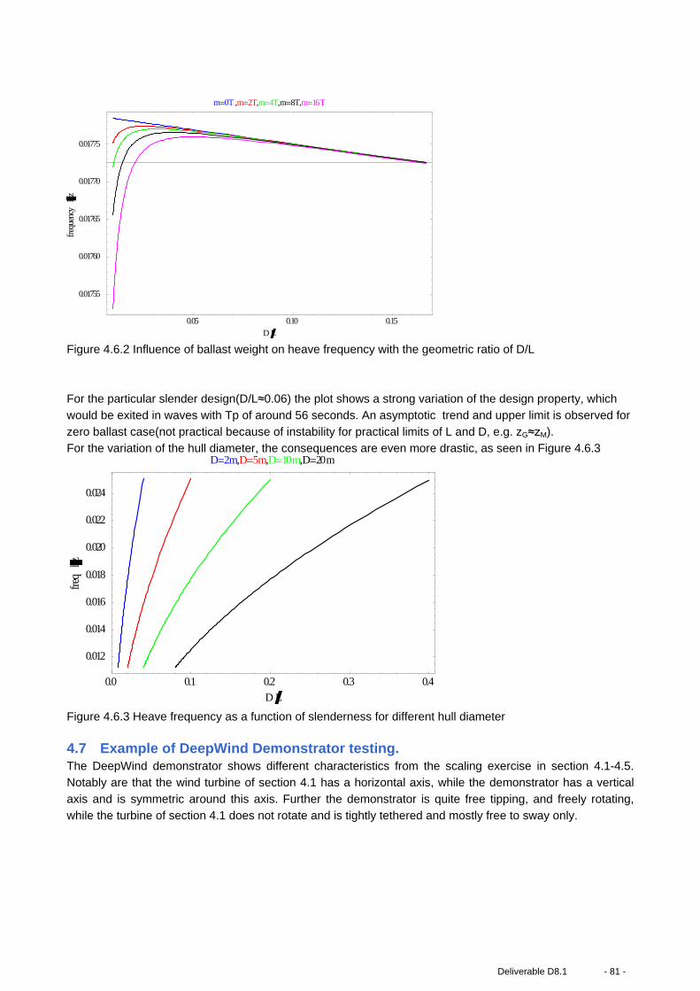
Figure 4.6.2 Influence of ballast weight on heave frequency with the geometric ratio of D/L
For the particular slender design(D/L≈0.06) the plot shows a strong variation of the design property, which
would be exited in waves with Tp of around 56 seconds. An asymptotic trend and upper limit is observed for zero ballast case(not practical because of instability for practical limits of L and D, e.g. zG≈zM). For the variation of the hull diameter, the consequences are even more drastic, as seen in Figure 4.6.3
Figure 4.6.3 Heave frequency as a function of slenderness for different hull diameter 4.7 Example of DeepWind Demonstrator testing. The DeepWind demonstrator shows different characteristics from the scaling exercise in section 4.1-4.5. Notably are that the wind turbine of section 4.1 has a horizontal axis, while the demonstrator has a vertical
axis and is symmetric around this axis. Further the demonstrator is quite free tipping, and freely rotating, while the turbine of section 4.1 does not rotate and is tightly tethered and mostly free to sway only.
0.05 0.10 0.15
0.01755
0.01760
0.01765
0.01770
0.01775
DL
frequ
encyHz
m0T ,m2T,m4T,m8T,m16T
0.0 0.1 0.2 0.3 0.4
0.012
0.014
0.016
0.018
0.020
0.022
0.024
DL
freqhz
D2m,D5m,D10m,D20m
Deliverable D8.1 - 81 -

The demonstrator is a 1 kW wind turbine as shown in Figure 4.7.1, and the properties to translate in surge and sway is not built in as a possibility for the demonstrator testing.
Figure 4.7.1 Left: Demonstrator heave, pitch, roll and yaw properties. Right: DOFs
The demonstrator has been tested in near to real conditions in Roskilde fjord[78.] (see Figure 4.7.2), and in the ocean laboratory of MARIN(NL)( see Figure 4.7.2.), with controlled waves, current and wind.
Figure 4.7.2 Left: Ocean lab testing of demonstrator at MARIN(NL). Right: Near to real tests in Roskilde
fjord(DK)[78.]
To conclude on scaling in section 4: for the testing it was important to simulate the motions and loads of the floating wind turbine correctly; the performance characteristics, but more important the thrust, of the wind turbine in the basin should be in-line with full scale. While for the underwater loads Froude scaling laws(see
simple scaling below) are used successfully in the offshore industry, the same could not be accomplished for the turbine blades. A particular deviation preventing ideal Froude scaling was that the demonstrator had to be equipped with a annular cap, enclosing the upper part of the tube(the conical part on the photo) for
being able to carry the rotor-floater.
- 82 - Deliverable D8.1
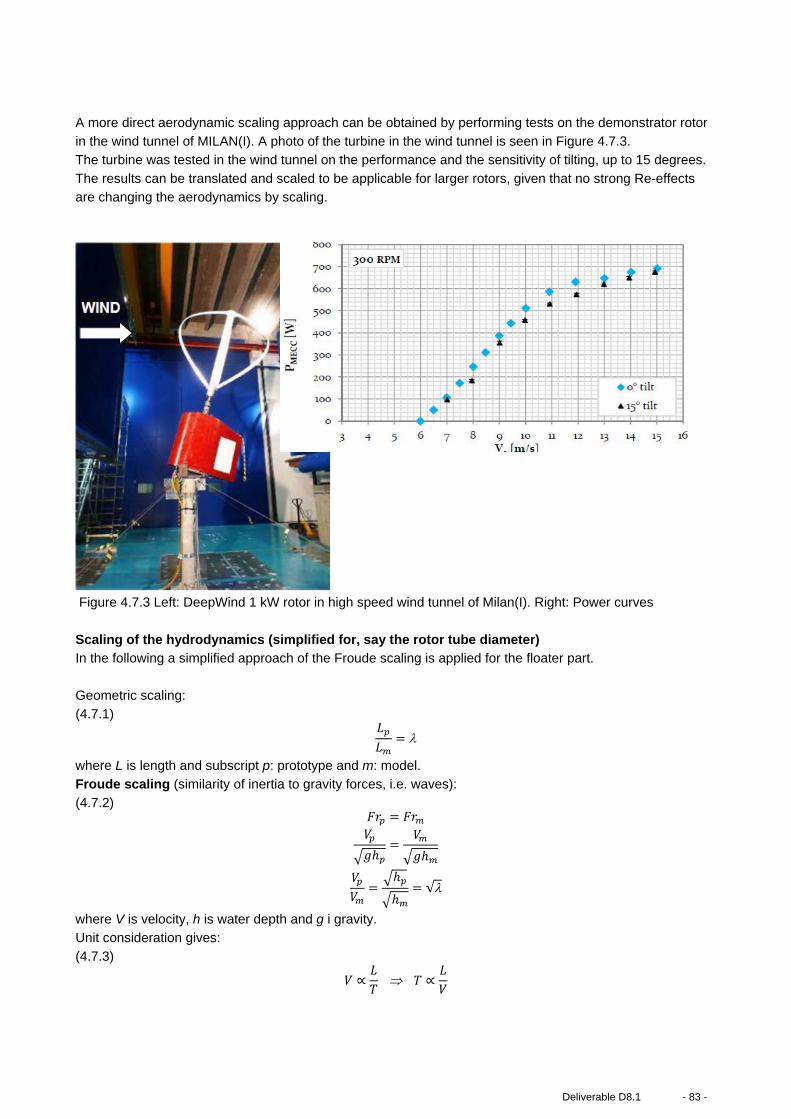
A more direct aerodynamic scaling approach can be obtained by performing tests on the demonstrator rotor in the wind tunnel of MILAN(I). A photo of the turbine in the wind tunnel is seen in Figure 4.7.3. The turbine was tested in the wind tunnel on the performance and the sensitivity of tilting, up to 15 degrees.
The results can be translated and scaled to be applicable for larger rotors, given that no strong Re-effects are changing the aerodynamics by scaling.
Figure 4.7.3 Left: DeepWind 1 kW rotor in high speed wind tunnel of Milan(I). Right: Power curves
Scaling of the hydrodynamics (simplified for, say the rotor tube diameter) In the following a simplified approach of the Froude scaling is applied for the floater part.
Geometric scaling:
(4.7.1) 𝐿𝑝
𝐿𝑚= λ
where L is length and subscript p: prototype and m: model. Froude scaling (similarity of inertia to gravity forces, i.e. waves):
(4.7.2) 𝐹𝑟𝑝 = 𝐹𝑟𝑚
𝑉𝑝
𝑔ℎ𝑝=
𝑉𝑚
𝑔ℎ𝑚
𝑉𝑝
𝑉𝑚=
ℎ𝑝
ℎ𝑚= √λ
where V is velocity, h is water depth and g i gravity. Unit consideration gives:
(4.7.3)
𝑉 ∝𝐿𝑇
⇒ 𝑇 ∝𝐿𝑉
Deliverable D8.1 - 83 -
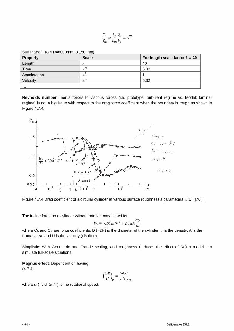
𝑇𝑝
𝑇𝑚∝
𝐿𝑝
𝐿𝑚
𝑉𝑚
𝑉𝑝= √λ
Summary:( From D=6000mm to 150 mm)
Property Scale For length scale factor λ = 40
Length λ 40
Time λ½ 6.32
Acceleration λ0 1
Velocity λ½ 6.32
…
Reynolds number: Inertia forces to viscous forces (i.e. prototype: turbulent regime vs. Model: laminar
regime) is not a big issue with respect to the drag force coefficient when the boundary is rough as shown in Figure 4.7.4.
Figure 4.7.4 Drag coefficient of a circular cylinder at various surface roughness’s parameters ks/D. [[76.] ]
The in-line force on a cylinder without rotation may be written
𝐹𝐷 = ½𝜌𝐶𝐷𝐷𝑈2 + 𝜌𝐶𝑀𝐴𝑑𝑈𝑑𝑡
where CD and CM are force coefficients, D (=2R) is the diameter of the cylinder, ρ is the density, A is the frontal area, and U is the velocity (t is time).
Simplistic: With Geometric and Froude scaling, and roughness (reduces the effect of Re) a model can simulate full-scale situations.
Magnus effect: Dependent on having
(4.7.4)
𝜔𝑅𝑈
𝑝
= 𝜔𝑅𝑈
𝑚
where ω (=2πf=2π/T) is the rotational speed.
- 84 - Deliverable D8.1

Note! This is similar to the tip-speed-ratio (TSR) applied in the aerodynamics. If Geometric and Froude scaling is applied then the Magnus effect should be identical in model and full-scale (prototype).
Issues: Scaling of the aerodynamics may require the rotational speed to be increased.
If the rotational speed is not scaled according to Froude scaling then R can be adjusted (Geometric scaling may be relaxed) to have the Magnus effect correct (at least in steady current). However, this affects the in-line force (and lift force without rotation), which means that the ratio between the Magnus effect and other
forces may not be correctly modelled. Also the buoyancy may be problematic. CD and CM also depend on a parameter known as the Keulegan-Carpenter number (KC = 2πa/D) where a is the amplitude of the wave motion (Figure 4.7.6). As seen scaling of the hydrodynamics without Geometric and Froude similarity is
challenging. A curiosity exists with the demonstrator, being manufactured with an aluminium tube diameter of 150mm. The Froude scaling suggests a diameter of this tube, e.g. the floater(at least if downscaled from 5 MW tube) of 150 mm. The tube was fitted with a 400 mm annular foam structure(see Figure 4.7.5) , and
mounted on the metallic part approximately 1/3 of the length of the underwater tube.
Figure 4.7.5 Photo of the tube and foam part
Deliverable D8.1 - 85 -
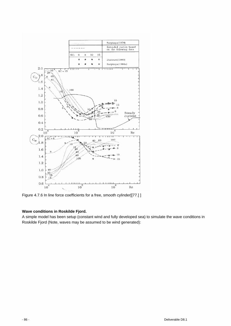
Figure 4.7.6 In line force coefficients for a free, smooth cylinder[[77.] ]
Wave conditions in Roskilde Fjord. A simple model has been setup (constant wind and fully developed sea) to simulate the wave conditions in
Roskilde Fjord (Note, waves may be assumed to be wind generated):
- 86 - Deliverable D8.1

Figure 4.7.7 Bathymetry The results suggest a significant wave height, Hs of up to 1m at RISØ with wind (20m/s) from 300°N
(direction with longest fetch)
Figure 4.7.8 Wave height for wind speed of 20m/s from 300 deg N
At the site (star in Figure 4.7.8) the significant wave height was measured to be Hs = 0.9m and Tp = 3.2 (describes the wave conditions assuming JONSWAP spectra (wind generated))
Deliverable D8.1 - 87 -

The shore protection manual5 gives simplified formulation to predict the wave height
Figure 4.7.9 Extract from Shore Protection Manual.
Equation (3-39) and (3-40) for h = 5m (water depth), wind speed = 20m/s and a fetch of 6 km (corresponding to a wind direction of 300°N) gives H = 0.9m and T = 3.1s. As seen these equation may be used to have a first estimate of the wave conditions in Roskilde Fjord for a given wind speed and direction.
By determining the fetch for each wind direction wave conditions can be forecasted. For now, the formulation in the Shore Protection Manual is expected to be sufficient, but the modern version may give a better estimate. However, this is also more cumbersome to implement.
Concluding remarks on scaling In spite of the similarities between the concepts of HAWTs and VAWTs with regards to similarity there are
obvious dis-similarities. Despite of this we can draw a number of conclusions:
• Scaling floating wind turbines for Reynolds and Froude effects is not achievable-practical considerations
are implemented such as floater scaling and Rotor scaling
• Magnus force is shown to be scaled properly via Froude scaling • The lowest eigenmode of DeepWind is dependent on ballast m, hull diameter D, draught L and ratio of
water density ρw and tubel density ρ.
5 http://www.archive.org/details/shoreprotectionm01unit, and modern version: http://chl.erdc.usace.army.mil/cemtoc
- 88 - Deliverable D8.1

Simulation results from comparison with measurements at MARIN The demonstrator has been tried implemented in the aeroelastic code Hawc2, to repeat the tests conducted in MARIN. In this first approach a simplified model has been implemented where all parts consist of beams with a given diameter, thickness and structural properties.
The water depth are not reported in [79.] or [80.] but is assumed to be h = 4.5m and therefore similar to the tests in Roskilde Fjord. A sketch of the demonstrator in HAWC2 is shown inFigure 4.7.10.
Figure 4.7.10 Sketch of demonstrator model in HAWC2.In the model the fork arm at P is modelled with a
simple hinge. The demonstrator has three degrees of freedom; heave, pitch and roll. Further the shaft can rotate with and defined rotational speed.
Deliverable D8.1 - 89 -
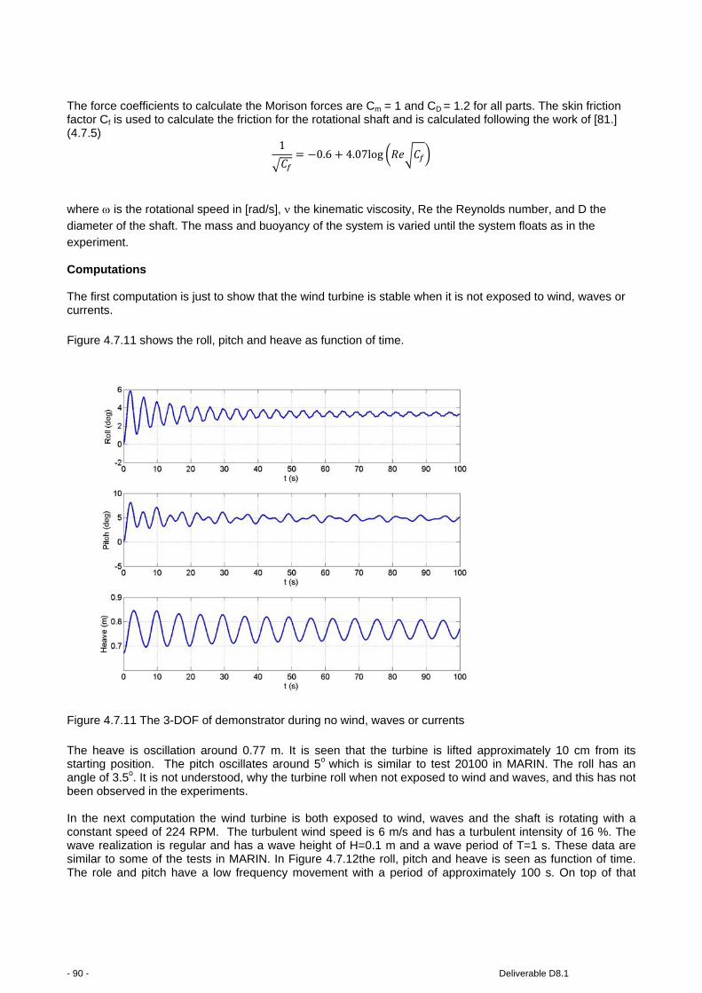
The force coefficients to calculate the Morison forces are Cm = 1 and CD = 1.2 for all parts. The skin friction factor Cf is used to calculate the friction for the rotational shaft and is calculated following the work of [81.] (4.7.5)
1𝐶𝑓
= −0.6 + 4.07log 𝑅𝑒𝐶𝑓
where ω is the rotational speed in [rad/s], ν the kinematic viscosity, Re the Reynolds number, and D the
diameter of the shaft. The mass and buoyancy of the system is varied until the system floats as in the experiment. Computations The first computation is just to show that the wind turbine is stable when it is not exposed to wind, waves or currents. Figure 4.7.11 shows the roll, pitch and heave as function of time.
Figure 4.7.11 The 3-DOF of demonstrator during no wind, waves or currents The heave is oscillation around 0.77 m. It is seen that the turbine is lifted approximately 10 cm from its starting position. The pitch oscillates around 5o
which is similar to test 20100 in MARIN. The roll has an angle of 3.5o. It is not understood, why the turbine roll when not exposed to wind and waves, and this has not been observed in the experiments. In the next computation the wind turbine is both exposed to wind, waves and the shaft is rotating with a constant speed of 224 RPM. The turbulent wind speed is 6 m/s and has a turbulent intensity of 16 %. The wave realization is regular and has a wave height of H=0.1 m and a wave period of T=1 s. These data are similar to some of the tests in MARIN. In Figure 4.7.12the roll, pitch and heave is seen as function of time. The role and pitch have a low frequency movement with a period of approximately 100 s. On top of that
- 90 - Deliverable D8.1

some high frequency oscillations are observed and also an oscillation with a period of approximately 6 s. This oscillation is also recognized in the heave motion. If the three motions are considered in frequency domain as in Figure 4.7.13 it is seen that the pitch and roll contains a little amount of energy at the wave frequency of 1 Hz. The energy at 0.16 Hz can be structural eigenfrequency, however this do not corresponds to the structural eigenfrequencies of the real demonstrator. Also the motions do not contain energy at 3.7 Hz which corresponds to the rotational speed of the shaft. This is different from what was seen in the tests in MARIN, where the forward and backward whirling also is seen. A more detailed set-up of the demonstrator in HAWC2 is therefore necessary to capture the same responses in the computations as in the tests.
Figure 4.7.12 The three degrees of freedom of the demonstrator as function of
time. Wind and waves are present and the shaft is rotation
Deliverable D8.1 - 91 -
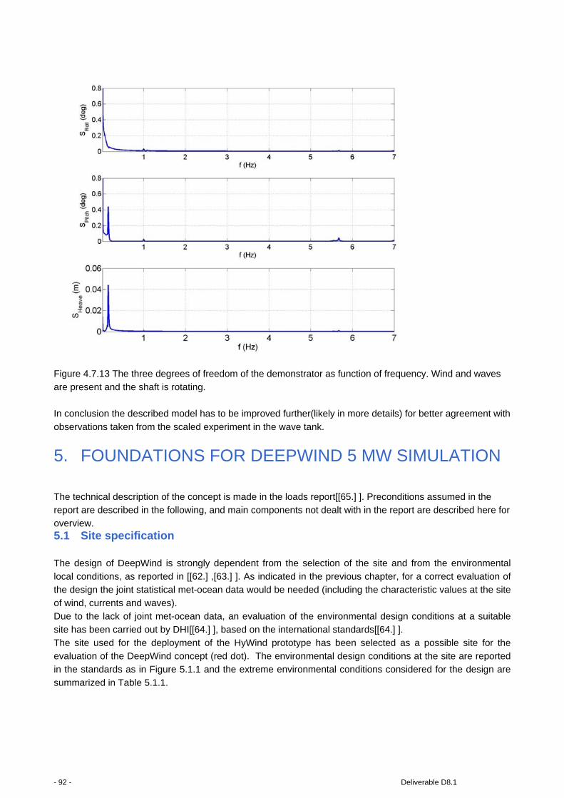
Figure 4.7.13 The three degrees of freedom of the demonstrator as function of frequency. Wind and waves
are present and the shaft is rotating. In conclusion the described model has to be improved further(likely in more details) for better agreement with
observations taken from the scaled experiment in the wave tank.
5. FOUNDATIONS FOR DEEPWIND 5 MW SIMULATION
The technical description of the concept is made in the loads report[[65.] ]. Preconditions assumed in the report are described in the following, and main components not dealt with in the report are described here for
overview. 5.1 Site specification
The design of DeepWind is strongly dependent from the selection of the site and from the environmental local conditions, as reported in [[62.] ,[63.] ]. As indicated in the previous chapter, for a correct evaluation of the design the joint statistical met-ocean data would be needed (including the characteristic values at the site
of wind, currents and waves). Due to the lack of joint met-ocean data, an evaluation of the environmental design conditions at a suitable site has been carried out by DHI[[64.] ], based on the international standards[[64.] ].
The site used for the deployment of the HyWind prototype has been selected as a possible site for the evaluation of the DeepWind concept (red dot). The environmental design conditions at the site are reported in the standards as in Figure 5.1.1 and the extreme environmental conditions considered for the design are
summarized in Table 5.1.1.
- 92 - Deliverable D8.1

Figure 5.1.1 Maximum 100 year tidal surface current [m/s](left). Significant wave height Hs and related
maximum peak period TP with annual probability of exceedance of 10-2 for sea-states of 3 h duration. ISO-curves for wave heights are indicated with solid lines while wave period lines are dotted, maps from [[64.] ].
Table 5.1.1 Most critical environmental conditions considered for the selected site, compare also the analysis of section 3, specifically 3.5. Note the limit wind speed is somewhat less than the 50 year find found in section 3.5.
Most critical environmental conditions at the site
Velocity of the water currents at the surface [m/s] 0.7
Maximum significant wave height Hs [m] 14
Maximum peak wave period TP [s] 16
Wind speed (limit wind speed of the design) [m/s] <25
For the simulation of the 5MW concept the above conditions have been applied and the details are reported in [[65.] ] with main components as i)rotor and column supporting the blades ii)floater, iii)generator and
torque absorption module, iv)mooring line system. The part iii) is equipped with buoyancy/ballast device that can be flooded and emptied by means of pressurized air contained as reservoir in the lower compartment of the floater. A sketch of the concept is shown in Figure 5.1.2 and in Figure 5.1.3. A power cable (inclusive
proper take off device-not shown), a standard naval solution for assisting buoys to distress the cable and the enclosure for the controls of the floating turbine are shown.
Also the low wind and wave situations as well as their duration are important, because these statistics influence the installation, maintenance &service, and the decommission expenses [e.g. 75]. With the relevant meteorological and oceanographic data such statics is fairly easy to compute, when eventually also the
conditions for offshore work and transport has been established for a specific wind turbine.
Deliverable D8.1 - 93 -

Figure 5.1.2 SolidWorks sketch of the 5 WM Baseline turbine©DTUWE
- 94 - Deliverable D8.1
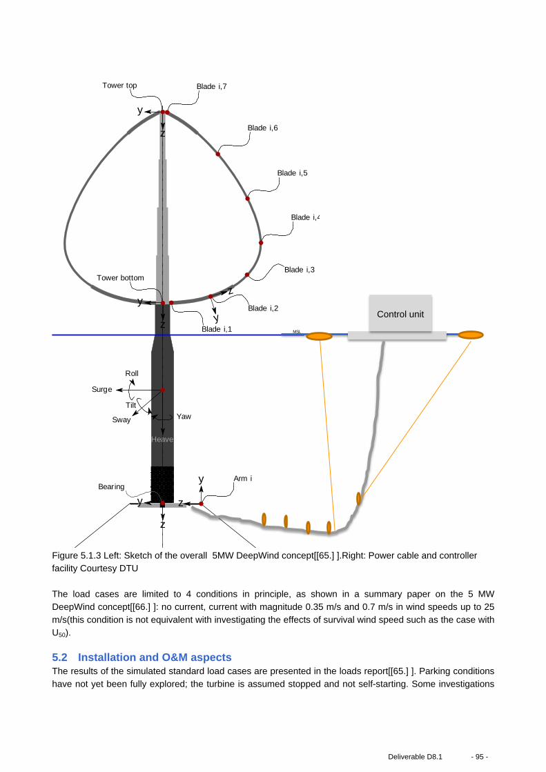
Figure 5.1.3 Left: Sketch of the overall 5MW DeepWind concept[[65.] ].Right: Power cable and controller facility Courtesy DTU
The load cases are limited to 4 conditions in principle, as shown in a summary paper on the 5 MW DeepWind concept[[66.] ]: no current, current with magnitude 0.35 m/s and 0.7 m/s in wind speeds up to 25
m/s(this condition is not equivalent with investigating the effects of survival wind speed such as the case with U50). 5.2 Installation and O&M aspects The results of the simulated standard load cases are presented in the loads report[[65.] ]. Parking conditions have not yet been fully explored; the turbine is assumed stopped and not self-starting. Some investigations
MSL
z
y
z
y
z
y z
y
z
y
Tower top Blade i,7
Blade i,6
Blade i,5
Blade i,4
Blade i,3
Blade i,2
Blade i,1
Tower bottom
BearingArm i
Heave
Surge
Sway
Roll
Yaw
Tilt
Control unit
Deliverable D8.1 - 95 -
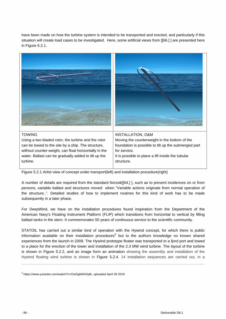
have been made on how the turbine system is intended to be transported and erected, and particularly if this situation will create load cases to be investigated. Here, some artificial views from [[66.] ] are presented here in Figure 5.2.1.
TOWING Using a two bladed rotor, the turbine and the rotor
can be towed to the site by a ship. The structure, without counter-weight, can float horizontally in the water. Ballast can be gradually added to tilt up the
turbine.
INSTALLATION, O&M Moving the counterweight in the bottom of the
foundation is possible to tilt up the submerged part for service. It is possible to place a lift inside the tubular
structure.
Figure 5.2.1 Artist view of concept under transport(left) and installation procedure(right) A number of details are required from the standard Norsok[[64.] ], such as to prevent incidences on or from
persons, variable ballast and structures moved when “Variable actions originate from normal operation of the structure..”. Detailed studies of how to implement routines for this kind of work has to be made subsequently in a later phase.
For DeepWind, we have on the installation procedures found inspiration from the Department of the American Navy's Floating Instrument Platform (FLIP) which transitions from horizontal to vertical by filling
ballast tanks in the stern. It commemorates 50 years of continuous service to the scientific community. STATOIL has carried out a similar kind of operation with the Hywind concept, for which there is public
information available on their installation procedures6 but to the authors knowledge no known shared experiences from the launch in 2009. The Hywind prototype floater was transported to a fjord port and towed to a place for the erection of the tower and installation of the 2.3 MW wind turbine. The layout of the turbine
is shown in Figure 5.2.2, and an image form an animation showing the assembly and installation of the
Hywind floating wind turbine is shown in Figure 5.2.4. 14 installation sequences are carried out, in a
6 https://www.youtube.com/watch?v=OwSgbW4Xptk, uploaded April 28 2010
- 96 - Deliverable D8.1

procedure of A-H steps involving crane equipment capable to erect and install heavy mass (rotor, turbine
tower section and nacelle) in heights.
Procedure for installation
In the following section we describe, how the DeepWind concept is supposed to be installed in 3 major
steps. To carry out the DeepWind installation, we do – in contrary to Hywind not intend to use a crane which
lifts the rotor and parts like nacelle into hub height, but rely on small vessels support with towing capacity
and a standard aft winding drum. There will be likely a need to have 1 small tugboat (probably one or two
extra for assisting), for towing of the floating system to the site from a port. It is supposed that the parts have
been built and assembled at the port.
At the intended site the wind and wave conditions have to be such that the floating wind turbine can be
erected by means of a procedure that controls the sinking of the device.
The Generator and torque absorption module is supposed to be assembled at the yard as well. The
complete structure is transported with a barge as indicated in Figure 5.2.5, and as indicated pontoons
connecting the cables( cable ends positioned on sea bed) are then positioned (the third assisting vessel is
possibly required). This procedure is required to be clearer in detail and execution because there is a need
to have control of the cables which in the end of the process needs to be tightened. It is not clear whether it
is better to have the turbine completely floating, or the end with the generator torque absorption module is
elevated on the barge as indicated in the figure. For this situation a boat crane or similar is used to lift the
end, or even the barge can be lowered in the water to release the turbine (part 2).The auxiliary equipment of
an assisting tugboat is supposed to tighten the cable sufficiently controlled in the process of erecting the
turbine. In the procedure, water ballast is added in a controlled way into the lowest part at the generator and
torque absorption module. During the procedures, camera assisted ROV’s are monitoring the process.
Divers equipped with deep sea diving gear and maintenance possibilities can assist the installation process
in situations where the control of the procedure has become critical.
Figure 5.2.2 Left: Hywind concept , Siemens 2.3 MW-82 turbine on a 65 m base ©Statoil .Right: Turbine at site in various wind conditions
Deliverable D8.1 - 97 -

In the loads report [[65.] ] simplified assumptions have been made for the installation procedure in order to
simulate the flipping from horizontal to vertical as a load case, which is to investigate if the structure is well
dimensioned against failure during erection? An example of the result from the stability investigation is
shown in Figure 5.2.3. It is seen from the figure, that the floater needs control during erection (moment
changes sign), and the static analysis recommends analysing the situation for the erection simulated in real
time. However this study has to be carried out in a future study of the design.
Figure 5.2.3 Moment of stability to counteract, for use of different sets of ballast to maintain a tilt angle.
- 98 - Deliverable D8.1

A
B
Deliverable D8.1 - 99 -

C
D
E
- 100 - Deliverable D8.1
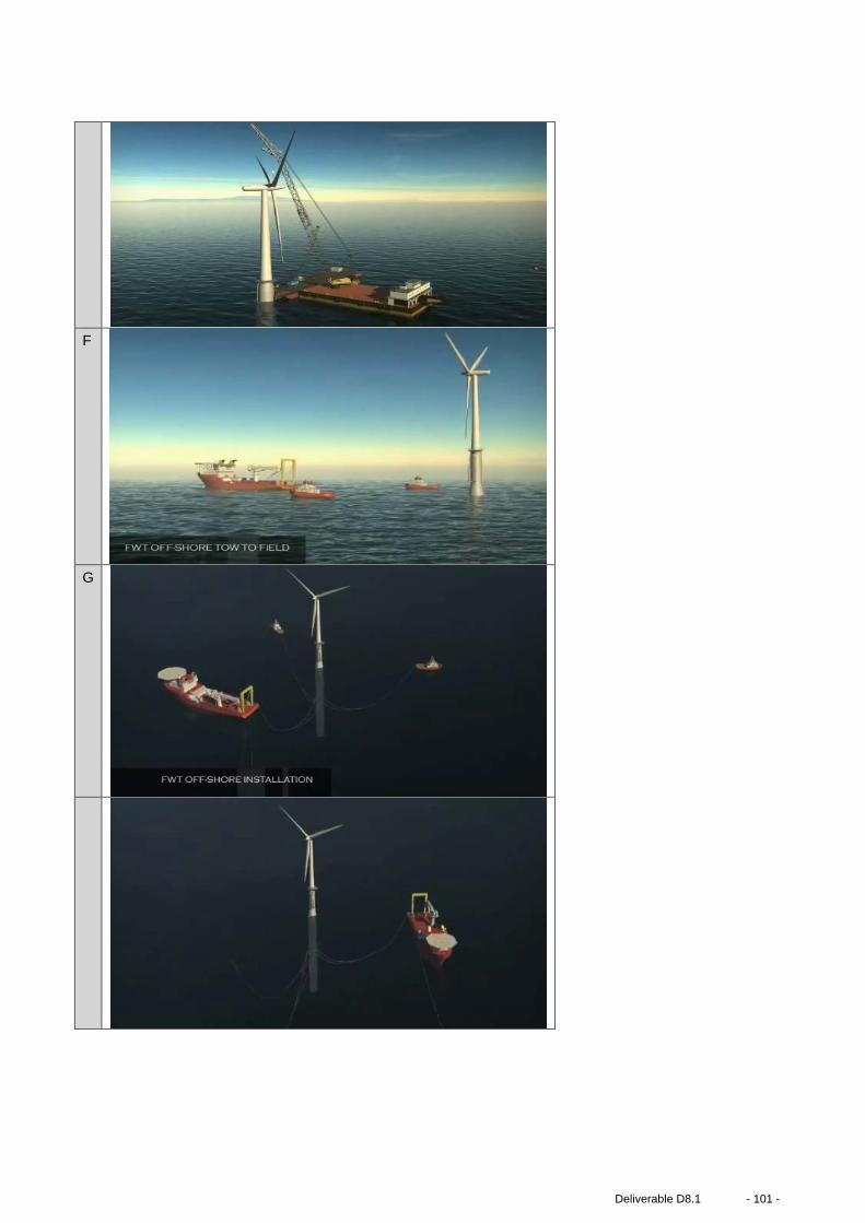
F
G
Deliverable D8.1 - 101 -
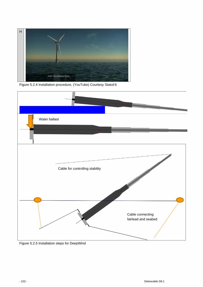
H
Figure 5.2.4 Installation procedure, (YouTube) Courtesy Statoil 6
Figure 5.2.5 Installation steps for DeepWind
Cable for controlling stability
Cable connecting fairlead and seabed
Water ballast
- 102 - Deliverable D8.1

O&M aspects The following suggestions are in nature theoretical and needs validation for improvement and progress. DeepWind is intended to provide as little as possible need for complicated equipment. This implies that
logistics are simplified with respect to volumes and masses that have to be dealt with in comparison with existing offshore wind turbine installation, operation and maintenance procedures. The modules are intended to be tolerant for failure, and underwater components will intentionally not need
replacement, since electronic equipment is placed in the controls enclose. However one or several Remotely Operated underwater Vehicles (ROVs) will be needed to carry out the acquisition part of the maintenance aspects. The ROV could be controlled remotely.
In case of maintenance- such as cleaning of marine growth developed at shallow depths of the rotating tube part, specialized tools (for example pressurized water jet) are needed as an attachment to the ROV. Workers can reside on a vessel during the maintenance.
In case of the failure of the power module, the reverse of the installation procedure is suggested. Lift bags are easily deployed and are intended to provide the necessary controls of the reverse process of installation.
Figure 5.2.6 Left: ROV type of operating environment. Right: ROV for deep sea remote assisted operations
Marine growth Marine growth (biofouling) leads to increased wave loading on structure due to increased effective diameter, as well as higher drag coefficient due to increased surface roughness. Other potential effects include
reduction in structural frequencies caused by additional non-structural mass and increased flow instability and vortex shedding (Schoefs & Boukinda 2004[[69.] ], Shi et al. 2012[[71.] ]). The type and severity of marine growth vary with geographic location, depth, salinity, temperature, current regime, nutrient and food
availability and oxygen concentration in water, as well as the structural design, its surface properties and type of installation (Whomersley & Pickens 2003[[73.] ], Shi et al. 2012[[71.] ]). In the North Sea mainly “hard growth” (mussels, barnacles) dominate in the upper 15-25 m of the water column, while “soft” growth (sea
squirts, sea anemones, sponges) tend to dominate at larger depth. Depending on water transparency macroalgae (soft growth) may populate surfaces from 5 m below surface to 30 m depth (Whomersley & Pickens 2003[[73.] ], Bruijs 2010[[70.] ]). Thickness in matured (after 6-10 years) marine growth may extend
up to 10-15 cm. Various methods are used to control marine growth including biocides (often Cu-based paint), enzyme-based coatings, mechanical (manual or automatic) removal of growth. Because of the potential fuel savings in the shipping industry new patents and products emerge every year. According to the
ISO-DIS-19901-1 standard[[74.] ], the Norwegian Sea has marine growth shown as in Table 5.2.1.
Deliverable D8.1 - 103 -

Other environmental impacts influencing drag may occur in parallel with marine growth, such as super-cooled water drops on the blades and tower structure.
Table 5.2.1 Marine Growth in the Norwegian Sea
Ports and logistics Providing capacity for the installation and O&M represents a part of the planning which requires investment. Offshore financing takes this action to be undertaken into consideration when the siting and power plant
project is planned as well. Establishment of yard site facilities and docks, warehouse, manpower and societal constraints are to be looked/planned for, changed/built or dealt with. It will depend on an actual case how to implement this, and such an implementation will be for study in future phases of the project.
5.3 Floater sensitivity analysis results for 5 and 20 MW Results from a sensitivity analysis carried out in the project [[68.] ] provide possibilities to look at variations from the base design in order to investigate the influence on the static and dynamic properties of the spar buoy, by varying some key parameters. The information is interpreted as a means to evaluate the 20 MW design, made from the point of scaling. The parameter variations are carried out on a 5 MW base design[[63.] ], varying one variable while keeping the other ones fixed. The following parameters were varied:
• Centre of gravity of the blades • Mass of blades • Mass of tower section above still water sea level
• Mass of generator • Water plane diameter • Main hull diameter
• Draught of spar hull
- 104 - Deliverable D8.1
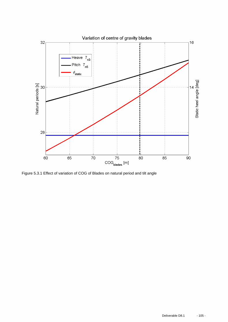
Figure 5.3.1 Effect of variation of COG of Blades on natural period and tilt angle
Deliverable D8.1 - 105 -

Figure 5.3.2 Effect of variation of blade mass on natural period and tilt angle
- 106 - Deliverable D8.1

Figure 5.3.3 Effect of variation of tower mass on natural period and tilt angle
Deliverable D8.1 - 107 -

Figure 5.3.4 Effect of variation of generator mass on natural period and tilt angle
- 108 - Deliverable D8.1

Figure 5.3.5 Effect of variation of diameter at SWL on natural period and tilt angle
Deliverable D8.1 - 109 -

Figure 5.3.6 Effect of variation of main hull diameter on natural period and tilt angle
- 110 - Deliverable D8.1

Figure 5.3.7 Effect of variation of floater draught on natural period and tilt angle
From the parametric variations, we may observe from Figure 5.3.8 that: 1. Increasing the centre of mass for the blades , say from 30 m(50%) increases the pitch stiffness period
by1.8 seconds( 6%) and increases the static heel(tilt) angle) with 4 degrees(36%). The changes are
most striking for the effect on the tilt angle 2. Increasing the blade mass from 100 T to 150 T(50%) or tower mass from 200 to 700 T(250%) increases
the pitch stiffness 8%and 33%, respectively and increases the pitch natural period by 8% and 33%,
respectively and for tilt with 33% and 400%, respectively. The most striking change happens for the tower tilt being highly progressive with tower mass parameter change. A fivefold increase of the blade mass provides approximate increases as for the tower, except for the tilt.
3. Increasing the generator mass with a factor of 9 from 50 T decreases the pitch stiffness 3% and reduces the pitch natural period by 1% and the tilt reduces 18%. In conclusion the floater is mostly affected on the tilt, and the result is similar as result showed for case 2). Increasing the water plane diameter
increases the pitch stiffness, and decreases the natural periods in heave 16.4 seconds, pitch by 2.5 seconds and tilt angle with 6 degrees, respectively.
4. Increasing the diameter at SWL from 4.5m with nearly 80%,a reduction of the heave period occurs with
43%, and lowering the pitch stiffness with 7%and reducing the tilt angle by almost 40%. The change has a significant influence on the natural periods and the tilt stability. A well-proportioned value of D1 will impact much on the floater cost and- capacity.
5. Increasing the main hull diameter from 7.5 m diameter by almost 50% increases the pitch stiffness, increases the heave natural period 10.4 seconds(≈40%) and decreases the pitch natural period by 7.7
Deliverable D8.1 - 111 -

seconds(24%) and the tilt angle with 22 degrees(≈80%), respectively. Again, here D2 has a significant influence on the floater cost and-capacity.
6. Increasing the spar draught from 95m with ≈40% the change will decrease the pitch stiffness by 5.7
seconds (≈20%) and increases the heave natural period by 4.2 seconds(≈20%) and decreases the tilt angle with ≈21 degrees(≈76%).
Figure 5.3.8 Sensibility analysis result
To avoid resonance motions of the spar buoy, the natural periods should be tuned to be larger than the wave
periods with significant energy. Increasing the pitch natural periods can be done by either increasing the mass moment of inertia (and added mass moment of inertia) or decreasing the stiffness. Decreasing the stiffness may have adverse effect on restoring the ”stability” of the system, e.g. it may result in excessive
heeling(tilt) of the platform. Lowering the centre of gravity would increase stability, and this can be achieved by (re)moving mass from the upper sections and add mass to the lower sections, below zG. The mass moment of inertia can be
increased by moving bulk of mass to the outer ends of the spar buoy, further away from zG. In particular, the results show that decreasing (or lowering) mass above zG and/or increasing mass below zG
increases the static pitch stability, but tends to decrease the pitch natural period. For the given parameter ranges, it appears that changes in moment of inertia does not compensate for the increased pitch stiffness which cause the pitch natural periods to decrease.
The report recommends that the natural period in heave is only affected by changes in total mass (mass and added mass) or water plane area.
From a point of increasing the power from 5 MW to 20 MW, the linear upscaling would provide a hull diameter around 16m, and a draught of 216m. A closer look up into the numbers from a estimation of the
buoyancy-weight stability vs pitch stability it seems more appropriate with a hull diameter of 10-11m. From
Case Variability From-to
% change Variability
Heave natural period Sec
Increase Sec(%)
Pitch natural period Sec
Increase Sec(%)
Tilt angle Deg
Increase Deg(%)
Centre of
gravity cogB[m]
60→90 50 29.4 1.8(6.1) 11.2 4(35.7)
Blade mass
mB[T]
100→150 50 29.8 2.4(8.1) 11.5 3.7(31.8)
Tower mass
mT[T]
200→700 250 25.6 8.4(32.8) 8.0 31.5(394.5)
Generator mass
mg[T]
50→500 900 31.4 -0.4(-1.3) 13.9 -2.4(-17.5)
Water plane
area diameter
D1[m]
4.5→8 78 38.5 -16.5(-
42.9)
32.5 -2.3(-7.1) 17.0 -6.0(-35.2)
Main hull
diameter D2[m]
7.5→11 47 25.6 10.4(40.6) 32.2 -7.7(-23.9) 26.4 -21.7(-
82.2)
Spar draught
L[m]
95→130 37 26.3 4.2(16.0) 33.7 -5.7(-16.9) 28.1 -21.4(-
76.2)
- 112 - Deliverable D8.1

the sensitivity analysis it appears that at least the hull diameter is within the range of synthesis from the figures(Figure 5.3.6), which shows that the pitch period decrease from 32 s to about 26 s. The detailed impacts from upscaling and the discussion of upscaling the concept from 5 to 20 MW is presented in a
different report, “Technological limits and possibility of upscaling to 20 MW (R)”.
6. CERTIFICATION ASPECTS
6.1 Overview of existing standards One could with good reason assume that the DeepWind concept might not be covered by any wind turbine standard since the design differs significantly from more traditional offshore wind turbines. However, the
standard normally used for design of horizontal axis turbines can to a large degree also be used for this particular concept with proper interpretation. Since the concept addresses a floating wind turbine, there are as a base point three important load simulation standards that can and shall be used for design specification
of the DeepWind concept. This consist of the IEC 61400-1 used for onshore turbines, IEC 61400-3 used for bottom fixed offshore turbines and IEC 61400-3-2 used for floating offshore turbines. The last standard is still at a draft stage and may very well be changed before fully finalized. Even though the standards cover all
kinds of wind turbines it is clear that the chosen load cases has been based on important situations for horizontal axis wind turbines (HAWT)’s and at least needs a special interpretation for application of vertical wind turbines.
Recently DNV has released their standard on floating offshore wind turbines, DNV-OS-J103(June 2013), and the IEC has launched a version(July 2014) for commenting on the same matter, IEV 61400-3-2 TS wind turbines-part 3-2: Design requirements for floating offshore wind turbines. There are also attempts to include
structural loads measurement requirements for vertical-axis wind turbines(VAWT)’s, in the IEC technical standard replacing IEC 61400-13 TS. Here, a short overview of the three common standards mentioned is given below with special emphasis on the load simulation requirements.
6.2 IEC 61400-1 ed. 3. Wind turbines part 1. Design requirements This standard has the purpose of establishing the overall safety level for onshore wind turbines with special
focus of environmental conditions, load cases needed to model 20years of operation loads and ensure that the turbine can withstand a storm with a recurrence period of 50years. Furthermore there are requirements to the general level of safety factors for the load and material as well as reference to other standard for the
detailed components used in a wind turbine e.g. generator or gearbox. The standard is the basis for load simulations of onshore wind turbines. In the standard a set of different
standardizes site conditions are set up mainly classified by a 50year storm wind speed and a turbulence class. When turbines are erected at a certain site it has to be demonstrated that the environmental conditions a more peaceful than the values used for the approved standard site. If some parameters exceed
the standard site conditions it has to be demonstrated that the load levels does not exceed the approved loads – this means a site specific approval.
A full set of load simulations requires both simulation of normal operation of the turbine in the wind speed range from cut-in to cut-out, start and stop situations, extreme wind conditions for both operation and stand still situations and fault condition on the turbine. Loads related to installation and service is also included. As
the standard is mainly intended for horizontal axis wind turbines, a significant part of the load case is devoted to different type of wind conditions with different levels of turbulence intensity and gusts of various kinds, whereas the loads related to e.g. installation and service is less specific specified.
Deliverable D8.1 - 113 -

The load cases covered by the IEC61400-1 are listed in Table 6.2.1. Simulations used for fatigue load analysis consists of normal power production combined with normal turbulent wind speed conditions (DLC
1.2), electrical fault situation combined with power operation in normal turbulent wind conditions (DLC 2.4) as well as normal start up, shut down and parked configuration. In DLC 2.4 all fault situations which does not cause a shut-down of the turbine should be included and the specific type of simulation therefore depends
on the actual turbine design. It could be a malfunctioning sensor causing a large yaw error, pitch error unless the probability of such failure is very low. As the simulations used for fatigue analysis includes stochastic turbulent wind conditions it is necessary to use a sufficient number of stochastic independent load simulation
for each wind speed, typically 6x10min simulations combined with yaw error to each side. The remaining load cases are used for extreme loads. This could be normal operation of the turbine in
extreme wind conditions (DLC 1.3, DLC 1.4, DLC 1.5), abnormal operation with a fault situation combined with either normal wind (DLC 2.1, DLC 2.2) or an extreme wind situation (DLC 2.3). Also start up, shut down, emergency shutdown and parked situations are investigated for extreme loads during extreme wind
conditions. There are also requirements for simulation of installation and service cases (DLC 8.1 and 8.2). For a typical
horizontal axis turbine the installation loads are assumed to be much less than for the remaining load cases, however it has to be documented that vortex induced vibration during installation (before the nacelle and rotor is installed) cannot occur or similar standstill vibrations when not all blades are mounted.
In general the number of load simulations for an onshore turbine is in the size of 1000 10min simulations, which requires quite fast simulation methods to be practically applicable.
- 114 - Deliverable D8.1

Table 6.2.1: Overview of load cases for an IEC61400-1 onshore certification
6.3 IEC 61400-3. Wind turbines part 3. Design requirements for offshore wind
turbines This standard consists of requirement to turbines and their substructures when used on offshore sites. This means that the turbine it-self first has to be certified with respect to the load cases and safety levels specified in IEC61400-1 and then also for the additional load cases and requirements specified in IEC61400-3.
Deliverable D8.1 - 115 -
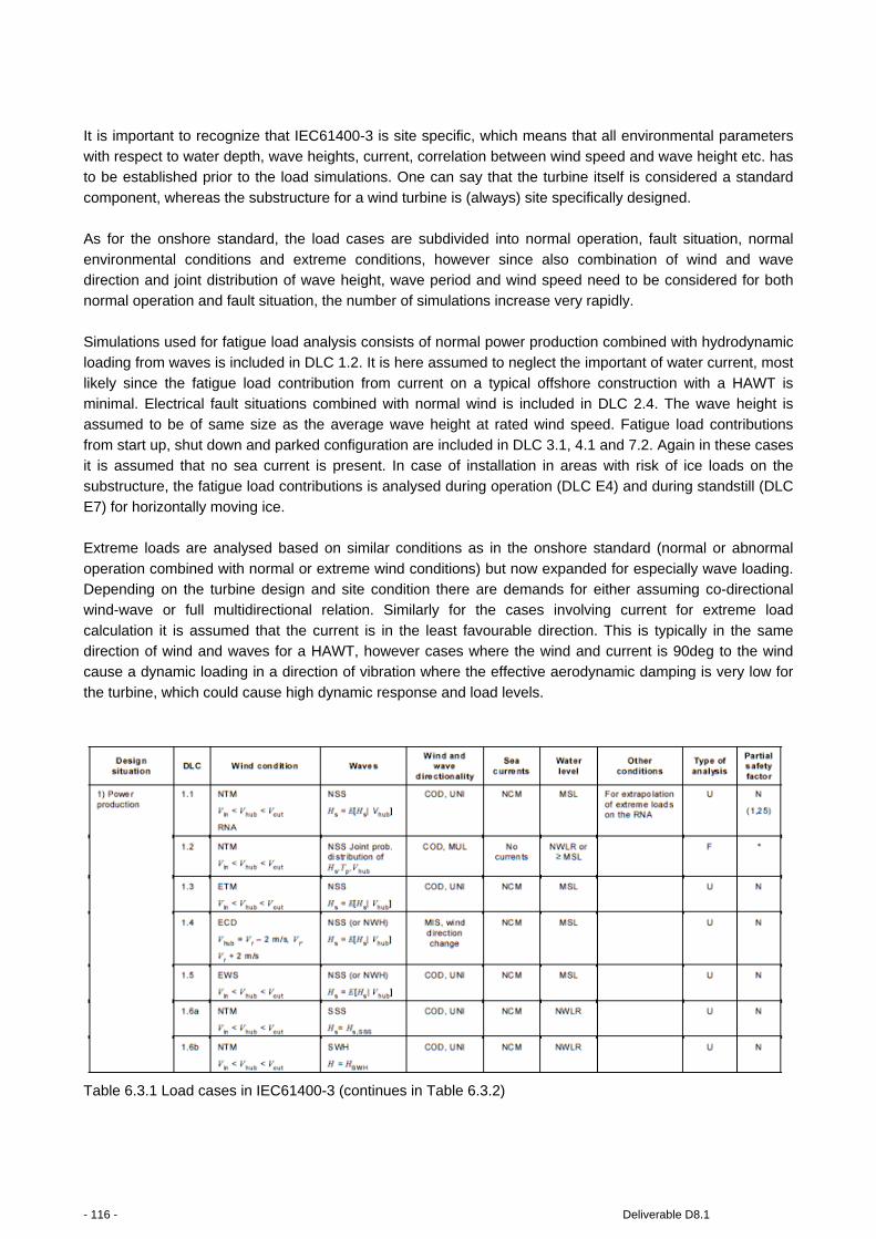
It is important to recognize that IEC61400-3 is site specific, which means that all environmental parameters with respect to water depth, wave heights, current, correlation between wind speed and wave height etc. has to be established prior to the load simulations. One can say that the turbine itself is considered a standard
component, whereas the substructure for a wind turbine is (always) site specifically designed. As for the onshore standard, the load cases are subdivided into normal operation, fault situation, normal
environmental conditions and extreme conditions, however since also combination of wind and wave direction and joint distribution of wave height, wave period and wind speed need to be considered for both normal operation and fault situation, the number of simulations increase very rapidly.
Simulations used for fatigue load analysis consists of normal power production combined with hydrodynamic loading from waves is included in DLC 1.2. It is here assumed to neglect the important of water current, most
likely since the fatigue load contribution from current on a typical offshore construction with a HAWT is minimal. Electrical fault situations combined with normal wind is included in DLC 2.4. The wave height is assumed to be of same size as the average wave height at rated wind speed. Fatigue load contributions
from start up, shut down and parked configuration are included in DLC 3.1, 4.1 and 7.2. Again in these cases it is assumed that no sea current is present. In case of installation in areas with risk of ice loads on the substructure, the fatigue load contributions is analysed during operation (DLC E4) and during standstill (DLC
E7) for horizontally moving ice. Extreme loads are analysed based on similar conditions as in the onshore standard (normal or abnormal
operation combined with normal or extreme wind conditions) but now expanded for especially wave loading. Depending on the turbine design and site condition there are demands for either assuming co-directional wind-wave or full multidirectional relation. Similarly for the cases involving current for extreme load
calculation it is assumed that the current is in the least favourable direction. This is typically in the same direction of wind and waves for a HAWT, however cases where the wind and current is 90deg to the wind cause a dynamic loading in a direction of vibration where the effective aerodynamic damping is very low for
the turbine, which could cause high dynamic response and load levels.
Table 6.3.1 Load cases in IEC61400-3 (continues in Table 6.3.2)
- 116 - Deliverable D8.1

Table 6.3.2 Load cases in IEC61400-3 (continues in Table 6.3.3)
Table 6.3.3 Load cases in IEC61400-3 (continues in Table 6.3.4)
Deliverable D8.1 - 117 -

Table 6.3.4 Ice load cases in IEC61400-3
- 118 - Deliverable D8.1
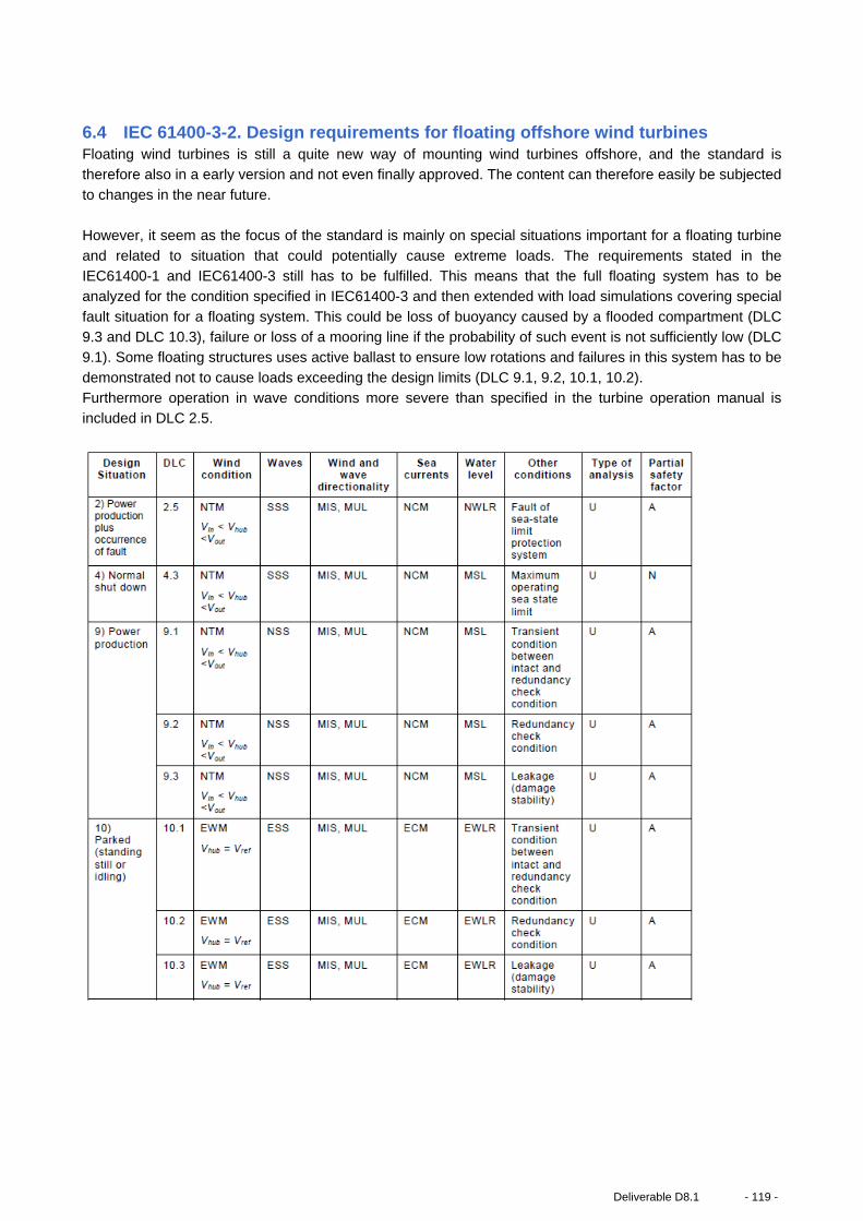
6.4 IEC 61400-3-2. Design requirements for floating offshore wind turbines Floating wind turbines is still a quite new way of mounting wind turbines offshore, and the standard is therefore also in a early version and not even finally approved. The content can therefore easily be subjected
to changes in the near future. However, it seem as the focus of the standard is mainly on special situations important for a floating turbine
and related to situation that could potentially cause extreme loads. The requirements stated in the IEC61400-1 and IEC61400-3 still has to be fulfilled. This means that the full floating system has to be analyzed for the condition specified in IEC61400-3 and then extended with load simulations covering special
fault situation for a floating system. This could be loss of buoyancy caused by a flooded compartment (DLC 9.3 and DLC 10.3), failure or loss of a mooring line if the probability of such event is not sufficiently low (DLC 9.1). Some floating structures uses active ballast to ensure low rotations and failures in this system has to be
demonstrated not to cause loads exceeding the design limits (DLC 9.1, 9.2, 10.1, 10.2). Furthermore operation in wave conditions more severe than specified in the turbine operation manual is included in DLC 2.5.
Deliverable D8.1 - 119 -

6.5 Experiences from previous VAWT projects Less sensitive to external wind conditions since the angle of attack variation caused by the rotor rotation is significantly larger than the perturbations caused by external gusts and turbulence. During operation the wind direction is also of no importance, which is however not the case during stand still. Since less VAWT turbines exist compared to HAWT turbines, there is less experience with the type of fault situations which could lead to extreme loads. In one report from Sandia [[84.] ] the experiences and lessons learned has been summarised. From this report it can be found that in some cases a Darrieus turbine (especially with a Troposkiien blade shape) experienced “the highest loads on the blades occurred during installation when the blades were lifted from the ground (before being bent into shape)”. Another experience was related to the stop situation of the wind turbine, which seems to have been problematic for most prototypes so far. “Many brake systems can provide time-varying torques between full off and full on. Stopping loads can be minimized by gradually applying the brakes. However, the braking schedule must be chosen very carefully to ensure that the brake pads do not overheat and lose their ability to stop the turbine. High blade loads can be experienced as the blades “ring” (at their natural frequency) back-and-forth about the tower when the tower first stops turning in a shutdown sequence. These loads can be minimized by releasing the brakes for a moment when the torque tube first stops, allowing the tower to turn with the blades, and then reapplying the brakes. Thus, programmable service brakes have a significant potential for reducing loads, but, again, the high capital costs and high maintenance of the brake system may preclude the inclusion of variable-torque braking system in future designs. The emergency brake set is usually overdesigned to ensure that it can stop the rotor in an over-speed event. The high torque loads on the rotor that are produced by such a full application of the emergency brakes can damage the rotor and power train, if they are not controlled properly.”
- 120 - Deliverable D8.1

6.6 Recommendations for load cases relevant for the DeepWind turbine In general it is concluded that the combination of load cases in IEC61400-1, IEC61400-3 and IEC61400-3-2 covers also design as the DeepWind concept. Special choices need to be taken for the specific concept
especially with respect to different fail situations that could occur. As the DeepWind concept is not equipped with any aerodynamic brake system, stop and emergency stop
situations is most likely the most important situation to investigate. A run-away situation will be fatal as for HAWT’s and severe dynamic transient loading may occur.
Normal operation is also a very important condition to simulate as these conditions are dimensioning for fatigue loads in general, especially the rotating tower and generator experience large loads during operation, whereas the impact on the blades may not be that critical due to the special load alleviating modified
Tropoidan shape. In general it is likely that many of the load cases including different kinds of extreme turbulence or gust are actually less important for the DeepWind than for the traditional HAWT design since the aerodynamic load variation caused by the rotation of the turbine itself is much higher that the additional
loads from turbulence and gusts. On the contrary, loads related to installation and service conditions may be way more important for the DeepWind concept than traditional HAWT’s. Here is especially thought of the turbine tilting during installation and generator service/repair and the installation of blades where they are
bend into place. Since one of the difficult issues with VAWT has been to predict the dynamic amplification of loads and
ensure that no resonance situations occurs, it is advisable that such a study is carried out prior to any load simulations. Especially if a variable speed concept is used it may not be trivial to ensure that no critical resonance occurs.
The IEC61400-1 has recently been extended regarding applicable methods for wake effects from neighbouring wind farms. Since the wake of a VAWT differs from a HAWT, the recommended methods may,
however, not be valid for VAWT wind farm configuration. The DeepWind concept is more sensitive to occurrence of water current that more traditional offshore
turbines seen so far; the IEC61400-3 may be conservative in its default recommendation of normal current profile, where the current is one-dimensional. However, it is stated in the standard that “Where appropriate and reliable measurements exist, site-specific current profiles may, however, be assessed as the basis of design and/or design verification of an offshore wind turbine”. This means that site specific current profiles may be used for the certification, which, however requires that these profiles are established on similar terms as the other site specific external conditions.
7. CONCLUSIONS and RECOMMENDATIONS
A description of the deep water conditions for the DeepWind site at the Western Coast of Norway, Karmøy has been provided and compared to the shallow and medium deep water conditions summarized in the Marinet report [46]. In particular the local current as part of local met-ocean conditions are compulsory
information for the loads determination and for cost studies. Real measurements exploring met-ocean data were not provided by Statoil for the project, and were replaced by model estimates and real data from a nearby site, Utsira Lighthouse .The scaling method proposed and demonstrated for HAWT is the dynamic-
Deliverable D8.1 - 121 -

elastic scaling, which maintains the ratios between hydrodynamic, aerodynamic, stiffness-induced and gravitational forces. This scaling preserves the Froude number for the water phase and the tip speed ratio for the rotor. The Reynolds numbers for air and water, however, are not conserved. A redesign of the model-
scale blades will therefore be needed. Here the scaled thrust-curve must be matched. Further, if possible, the torque from the airfoil should be matched. This requirement, however, is difficult to achieve due to the change in lift/drag ratio at low Reynolds number. It is therefore foreseen, that the aerodynamic torque and
thus produced power will not be scaled correctly. As a consequence, roll-forcing induced by the dynamic change in generator moment will not scale correctly. However, the correct scaling of rotor thrust is found to have higher priority and thus justifies the scaling choice.
An example of down-scaling of wind and wave conditions has been supplied. The example also demonstrates how the structure (a floating wind turbine) should be scaled. It is demonstrated that the
proposed scaling yields model-scale results for thrust- and wave- induced motion that can be up-scaled to prototype scale with a perfect match.
In summary, we conclude that the wind conditions as found in section 2.4 and at the demo-site are quite similar as far as can be judged from the respective analyses. The wave climate on the other hand seems more severe at the DeepWind site, especially with respect to more extreme events, which is probably to be
expected, given the greater water depth and the large fetch possibilities for this site. A DeepWind model is presented with capacity to model heave, surge and pitch of the rigid body system with
an elastic mooring line system. With the model the connection with the scaling is shown for a rigid body motion.
A comparison with a 1 kW proof-of-principle demonstrator is shown as an example of performing exercises in to validate simulations and measurements carried out in the oceanic laboratory(and under near-to-real conditions in Roskilde Fjord) and to describe the progress for simulating a small floating offshore wind
turbine subjected to certain test conditions. The DeepWind concept is described in terms of what inputs and constraints there have emerged and some
illustration of how installation, O&M will affect loads and logistics, and cost. Standards and codes, mainly IEC codes on offshore wind turbines have been surveyed and commented on
the use for VAWTs. In conclusion, recommendations for load case investigation are provided.
- 122 - Deliverable D8.1

References
[1.] UpWind: Fisher, T., W. deVries and B. Schmidt: UpWind deliverable, Design Basis WP4: Offshore Foundations and Support Structures - UpWind Project. Universität Stuttgart, 2010.
[2.] IEC 61400-3: Wind turbines- Part 3: Design of offshore wind turbines, 2009
[3.] DNV-OJ-J101. OFF SHORE STANDARD: Design of offshore wind turbine structures. DNV,
2007.
[4.] ABS(American Bureau of Shipping), Offshore Wind Turbine Installation, American Bureau of
Shipping, 2010
[5.] ABS(American Bureau of Shipping), Design Standards for offshore wind farms, American
Bureau of Shipping, 2011
[6.] IEC 61400-1, Design requirements, 2008.
[7.] IEC 61400-1, Design requirements-amendment1, 2010
[8.] DS/EN 61400-3, Wind turbines-Part 3: Design requirements for offshore wind turbines, 2009.
[9.] J.Mann, Wind field simulation, Prob. Engng. Mech. Volume 14, no 4, 269-282, 1998
[10.] E.R. Jørgensen, S.E. Larsen, S. Frandsen, N.J. Tarp-Johansen and Jenny Trumars, Beatrice Environmental data, Risø-I-2354- FP6 Integrated project DOWNVInd- contract 503202.
[11.] S. E. Larsen, N. E. Tarp-Johansen, S. Frandsen and E. R. Jørgensen, Södra Midsjöbanken
Environmental Data-Initial analysis, Risø-I-2505. FP6 Integrated project DOWNVInd- contract 503202
[12.] Pena, T. Mikkelsen, S.E. Gryning, C.B. Hasager, A.N. Hahmann, M. Badger, I. Karagali and M.
Coutney, Offshore vertical wind shear. Final report NORSEWIND work task 3,1, DTU Wind Energy reort 0005 (EN), 2012
[13.] N. Hahmann, Julia Lange, Alfredo Peña and Charlotte B. Hasager: The NORSEWInD numerical
wind atlas for the South Baltic, DTU Wind Energy-E-Report-0011(EN).
[14.] Karagali, A. Pena, M. Badger and C.B. Hasager, Wind characteristics of the North Sea and the
Baltic Seas from QuickScatt satellite. Wind Energy. 2012
[15.] B M Sumer and J Fredsøe "Hydrodynamics around cylindrical structures". World Scientific 2006.
[16.] Wierings, J.” Shapes of annual frequency distributions of wind speed observed on high
meteorological masts. Bound-Layer Meteorol,1988,47,85
[17.] M.K. Ochi. Ocean waves: the stochastic approach. Cambridge Ocean Technology Series, 2005.
[18.] Y. Goda. Random Seas and Design Of Maritime Structures. Advanced Series On Ocean Engineering, Volume 15 - World Scientific Publishing Company, 2000.
Deliverable D8.1 123
[19.] O. Ditlevsen. Stochastic model for joint wave and wind loads on offshore structures. Structural Safety, 24:139163, 2002.
[20.] P.W. Cheng, G.J.W. van Bussel, G.A.M. van Kuik, and J.H. Vugts. Reliability-based design
methods to determine the extreme response distribution of offshore wind turbines. Wind Energy, 6:122, 2003.
[21.] K. Johannessen. Joint distribution for wind and waves in the northern north sea. In Proceedings
of the Eleventh International Offshore and Polar Engineering Conference, 2001.
[22.] P. Agarwal, L. Manuel. Simulation of offshore wind turbine response for long-term extreme load
prediction. Engineering Structures, Volume 31, Issue 10, October 2009, Pages 2236-2246
[23.] Hildebrant and T. Schlurmann: Breaking wave kinematics, local pressure, and forces on a tripod support structure. Coastal Engineering,1-14, 2012.
[24.] O. J. Andersen and J. Løvseth: The Frøya database and maritime boundary layer wind
description. Science Direct Marine Structures, 173-192. 2006.
[25.] O. J. Andersen and J. Løvseth: Stability modifications of the Frøya wind spectrum. Journ. Wind
Engeneering Industrial Aerodynamics, 236-242, 2010.
[26.] O. J. Andersen and J. Løvseth: Gale force maritime wind. The Frøya data base. Part1: Sites and instrumentation. Review of the data base. Jour. Wind Engeneering Industrial Aerodynamics, 97-109, 1995
[27.] Bottasso, Carlo. "Development of a Wind Tunnel Model for Supporting Research on Aero-Servo-
Elasticity and Control of Wind Turbines." Diss. Politecnico di Milano, 2011.
[28.] Wolowicz , Chester, James Bowman, and William Gilbert. United States of America. NASA. Similitude Requirements and Scaling Relationships as Applied to Model Testing (NASA Technical Paper 1435). Hampton, Virginia: Langley Research Center, 1979.
[29.] Martin, Heather. METHODOLOGY FOR WINDin/WAVE BASIN TESTING OF FLOATING
OFFSHORE WIND TURBINES. University of Maine, June 10-15 2012.
[30.] Singleton, Jeffrey. "IMPORTANT SCALING PARAMETERS FOR TESTING MODEL-SCALE
HELICOPTER ROTORS." Diss. U.S. Army Research Laboratories, Vehicle Technology Center NASA Langley Research Center.
[31.] Newman, John Nicholas. Marine Hydrodynamics. 1. Cambridge: MIT Press, 1977.
[32.] Dagher, Habib. "Floating Offshore Wind". University of Maine, DeepCwind Consortium. 27 Apr.
2011. Advanced Structures & Composites Center. 25 June 2012.
[33.] Hall, Stephen. "Dynamic Modelling." Sport Aviatioin. July 1987: 288 - 298.
[34.] Jameson, Peter. Innovation on Wind Turbine Design. Sussex: John Wiley and Sons Ltd., 2011.
78.
[35.] Anderson, John. Fundamentals of Aerodynamics. 4th. Singapore: McGraw-Hill, 2007. 41, 499.
[36.] Jain, Anant, Amy Robertson, Jason Jonkman, Andrew Goupee, Richard Kimball, and Andrew
Swift. United States of America. U.S Department of Energy. FAST Code Verification of Scaling
124 Deliverable D8.1

Laws for DeepCwind Floating Wind System Tests. Oak Ridge, TN: Office of Scientific and Technical Information, 2012.
[37.] Jonkman, J.M. "Dynamics Modelling and Loads Analysis of an Offshore Floating Wind Turbine."
Diss. National Renewable Energy Laboratory, 2007.
[38.] Hansen, AM and Laugesen R “Experimental study of the dynamic response of a TLP wind turbine”. BSc thesis, DTU Mechanical Engineering. Lyngby, Denmark, June 2012.
[39.] Jonkman, J, Butterfield, S, Musial, W, Scott, G. “Definition of a 5 MW reference wind turbine for
offshore system development”. NREL, US, 2009.
[40.] Matha, D. “Model development and loads analysis of an offshore wind turbine on a tension leg
platform with a comparison to other floating wind turbine concepts”. MSc thesis. Univ. Colorado, US. April 2009.
[41.] Hansen, MOL “Aerodynamics of wind turbines”. Earthscan, London, UK, 2008.
[42.] Larsen, TJ and Hanson, TD “A method to avoid negative damped low frequency tower vibrations
for a floating pitch controlled wind turbine”, Proc. Science Torque Wind. 2007.
[43.] M Kühn, "Dynamics and design optimisation of offshore wind energy conversion systems," PhD
Thesis, Delft University of Technology, Delft, The Netherlands. 2001.
[44.] J.N. Newman, Marine Hydrodynamics, 1977, MIT Press
[45.] Morison JR, O’Brien MP, Johnson JW and Schaaf SA “The forces exerted by surface waves on piles”. J. Petrol. Techn., Petroleum Transactions, AIME 189 pp 149-154. 1950
[46.] Bredmose,H., Larsen.S.E.,Matha,D.,Rettenmeier,A.Mosino,E.Saetrau,L.Collation of offshore
wind-wave dynamics. MARINET report ,50p.2012.
[47.] Søren Larsen: Micro Scale Meteorology-Lecture notes, Wind Energy I Report 1850(En). DTU Wind Energy.
[48.] R. Stull.: An Introduction to Boundary Layer Meteorology (Atmospheric Sciences Library) 1991
[49.] Dee D. P., et al., “The ERA-Interim reanalysis: configuration and performance of the data
assimilation system,” Quarterly Journal of the Royal Meteorological Society, vol.137, Issue 656,
pp.553–597, Apr. 2011.
[50.] Hahmann A. N., D. Rostkier-Edelstein, T.T. Warner, F. Vandenberghe, Y. Liu, R. Babarsky and
S.P. Swerdlin, “A reanalysis system for the generation of mesoscale climatographies,” Journal of Applied Meteorology and Climatology, vol.49, no.5, pp.954-972, May 2010.
[51.] Marinelli, M,, P. Maule, A. Hahmann, O. Gehrke, P. B. Nørgård, N. Cutululis, Wind and Photovoltaic Large –scale regional models for hourly production evaluation. Paper TSTE-00523-2013.R1, to appear IEEE Transaction on Sustainable Energy, 2014
[52.] Mark Kelly · Ib Troen · Hans E. Jørgensen, Weibull-k Revisited: “Tall” Profiles and Height
Variation of Wind Statistics, Boundary-Layer Meteorology, 152:107–124, DOI 10.1007/s10546-
014-9915-5, 2014
Deliverable D8.1 125

[53.] Larsén X. G., Ott S, Badger J., Hahmann A. H. and Mann J. Recipes for correcting the impact of
effective mesoscale resolution on the estimation of extreme winds. J. Appl. Meteorol. Climat., 51(3):521–533, 2012.
[54.] Larsén X. G., Extreme wind mapping for Hornsea wind farm, Wind Energy Report-I-0040. 2013a
[55.] Larsén X. G., Extreme wind mapping over the North Sea, Wind Energy Report-I-0047. 2013b
[56.] Larsén X., Badger J., Hahmann A. N. and Mortensen N.G. 2013: The selective dynamical downscaling method for extreme wind atlases, Wind Energy 16:1167-1182, DOI:10.1002/we.1544.
[57.] Larsén X.; Mann, J.; Rathmann, O.; Jørgensen, H. 2014: Uncertainties of the 50-year wind from
short time series using generalized extreme value distribution and generalized Pareto
distribution, Wind Energy (ISSN: 1095-4244) (DOI: http://dx.doi.org/10.1002/we.1683), published online.
[58.] Mellor G. L. and T. Yamada, “Development of a turbulence closure model for geophysical fluid problems,” Reviews of Geophysics, vol.20, no.4, pp. 851-875, Nov. 1982.
[59.] Saha S. and Co-authors. The NCEP climate forecast system reanalysis. American Meteorological Society, BAMS, pages ES9–ES25, 2010a.
[60.] Saha S. and Co-authors. Supplement to the NCEP climate forecast system reanalysis. American Meteorological Society, BAMS, pages 1015–1057, 2010b.
[61.] Wang W., C. Bruyere, M. Duda, J. Dudhia, D. Gill, H-C. Lin, J. Michaelakes, S. Rizvi and X.
Zhang, “WRF-ARW Version 3 Modelling System User’s Guide,” Mesoscale & Microscale Meteorology Division, National Center for Atmospheric Research, Boulder, USA, 2009.
[62.] Luca Vita, "Offshore floating vertical axis wind turbines with rotating platform," Risø DTU,
Roskilde, Denmark, PhD dissertation PhD-80, 2011.
[63.] L. Vita et al., "A novel concept for floating offshore wind turbines: recent developments in the
concept and investigations on fluid interaction with the rotating foundation," in Proceedings of the International Conference on Ocean Offshore and Arctic Engineering (OMAE), Shanghai, China, 2010.
[64.] S. Carstensen, "DeepWind test plan (Milestone 11)," DHI (Danish Hydraulic Institute), 256769-
DeepWind, 2011.
[65.] Norsok standard N-003 Ed.2, "Actions and action effects," 2007.
[66.] Knud A. Kragh, Helge Aagaard Madsen, and David R.S. Verelst “2nd Iteration Design Loads for
the DeepWind 5MW Turbine” Draft version 16/4 2014 DTU Wind Energy Report-XXXX(EN)
[67.] U. S. Paulsen et al.:”The 5 MW DeepWind floating offshore vertical wind turbine concept design-status and perspective” Paper EWEA2014, Barcelona Spain Schoefs F & Boukinda M. (2004)
126 Deliverable D8.1
[68.] Sizing of a Spar-type floating support structure., D5.1 report for the European Commission, DeepWind. 82 pages. 2014
[69.] Modeling of marine growth effect on offshore structures loading using kinematics field of water
particle. Proceedings of the International Offshore and Polar Engineering Conference, pp. 419-426
[70.] Bruijs, MCM (2010) Survey of marine fouling on turbine support structures of the offshore
windfarm Egmond aan Zee (Prepared for Noordzeewind by KEMA Technical & Operational Services), p.36.
[71.] W Shi, H-C Park, J-H Baek, C-W Kim, Y-C Kim and H-K Shin (2012) Study on the marine growth
effect on the dynamic response of offshore wind turbines. Internat. J Precision Eng. & Manufac. 13: 1167-1176.
[72.] Dürr S and JC Thomason (2010) Biofouling. Blackwell Publishing Ltd.
[73.] Whomersley P & GP Pickens (2003) Long-term dynamics of fouling communities found on
offshore installations in the North Sea. J Mar Biol Ass UK 83: 897-901
[74.] Olsen SM, Pedersen LT, Laursen MH, Kiil S & K Dam-Johansen (2007) Enzyme-based antifouling coatings: a review. Biofouling 23: 369-383
[75.] Petroleum and natural gas industries — Specific requirements for offshore structures —Part 1:
Metocean design and operating considerations. ISO/DIS 19901-1 2013
[76.] Achenbach,E. and Heinecke, E. On vortex shedding from smooth and rough cylinders in the
range of Reynolds numbers 6 ×10³ to 5 ×10⁶ . Journal of Fluid Mechanics, 109:239-251,1981.
[77.] B.M.Sumer and J. Fredsøe (1999) “Hydrodynamics around cylindrical structures”, Advanced Series on Coastal Engineering – Volume 12
[78.] DeepWind 1 kW Demonstrator Tests in Roskilde Fjord. DTU Wind Energy E-0053 August 2014
49 pp
[79.] MARIN. FP7 program deepwind - model test vertical wind turbine. data report. Technical Report 24662-1-OB Volume II, MARIN, March 2013.
[80.] A. Tesauro, T.F. Pedersen, and C. B. M Pedersen. Deepwind demonstrator testing at Marin
facility,8-12 March 2013 - data report. Technical Report E-0034, DTU Wind Energy, August 2013.
[81.] Theodore Theodorsen and Arthur Regier. Experiments on drag of revolving disks, cylinders, and
streamline rods at high speeds. Technical Report NACA-TR-793, National Advisory Committee for Aeronautics. Langley Aeronautical Lab.; Langley Field, VA, United States, 2044
[82.] BVG associates, 2012: Offshore wind cost reduction pathways: Technology work stream, May
2012, 232 p
[83.] Donelan M. A. et al (2004) On the limiting aerodynamic roughness of the ocean in very strong
winds Geophysical Research Letters, vol. 31, L18306.
[84.] Sutherland, H.J., Berg, D.E., and Ashwill, T.D., “A Retrospective of VAWT Technology,” Sandia
National Laboratories Technical Report, SAND2012-0304, January 2012.
Deliverable D8.1 127

Acknowledgements
Ole Svenstrup Pedersen, Dr., MSc. in Environmental Engineering. Head of Research in Coastal and Estuarine Engineering, Danish Hydraulic Institute (DHI) Denmark’s DHI Head Office. Ole has kindly provided
the HINDCAST data and information for the DeepWind site, has reviewed the section and kindly contributed on marine growth in the report.
Henrik Bredmose, Dr. Associate professor in Offshore Wind Energy at DTU Wind Energy at the Technical University of Denmark. Henrik has kindly suggested the chapters for the literature survey and foundations for the shallow offshore met-ocean part, and collecting the information about scaling.
Birgitte Furevik, Dr. Associate professor in the department of Research and Development at the Norwegian Meteorological Institute. Birgitte has kindly provided us with the met-ocean data obtained at Utsira Fyr
nearby Karmøy. Lorenzo Battisti, Dr Associate Professor at the University of Trento, Mechanical and Civil Engineering
Department . Lorenzo and his team(Alessandra Brighenti, Enrico Benini) have contributed with wind tunnel measurements to additional understanding of the aerodynamics of the VAWT rotor and with vortex and BEM codes on the calculation of VAWT rotors.
I will also like to thank DTU for support and colleagues in DTU Wind Energy for constructive feedback, discussions and technical help wherever needed. A special thanks to Dr. Søren Larsen for constructive
discussions and response implementations in the report. The material being released is based on reports provided for the DeepWind, MARINet, NorseWind,
DOWNVInD , Twenties, and UpWind projects all provided under EU actions.
128 Deliverable D8.1

DTU Wind Energy is a department of the Technical University of Denmark with a unique integration of research, education, innovation and public/private sector consulting in the field of wind energy. Our activities develop new opportunities and technology for the global and Danish exploitation of wind energy. Research focuses on key technical-scientific fields, which are central for the development, innovation and use of wind energy and provides the basis for advanced education at the education. We have more than 240 staff members of which approximately 60 are PhD students. Research is conducted within nine research programmes organized into three main topics: Wind energy systems, Wind turbine technology and Basics for wind energy.
Technical University of Denmark
Department of Wind Energy
Frederiksborgvej 399
Building 118
4000 Roskilde
Denmark
Telephone 46 77 50 85
www.vindenergi.dtu.dk