Computing the Stereo Matching Cost with aConvolutional Neural Network

Seminar Recent Trends in 3D Computer Vision

Markus HerbSupervisor: Benjamin Busam

Chair for Computer Aided Medical ProceduresTechnische Universitat Munchen

Abstract. This paper presents a novel approach to the problem of com-puting the matching-cost for stereo vision. The approach is based upona Convolutional Neural Network that is used to compute the similarityof input patches from stereo image pairs. In combination with state-of-the-art stereo pipeline steps, the method achieves top results in majorstereo benchmarks. The paper introduces the problem of stereo match-ing, discusses the proposed method and shows results from recent stereodatasets.

1 Introduction

3D depth perception has been a long term goal within computer vision withstereo vision in particular being an area of research for several decades [1,2].The objective in stereo vision is to reconstruct the 3D depth information ofa scene from the input images of two cameras at different viewpoints and theknown camera geometry.

Despite the fact that great progress has been made over the years in thisfield, the topic continues to be an active area of research. This is largely dueto the great number of potential applications, especially in robotics, such asautonomous driving, but also for medical applications including surgical roboticsor X-ray imaging. While there exist alternative approaches to depth-perception,such as RGB-D cameras including the Microsoft Kinect, stereo vision is especiallyappealing since it only depends on passive camera sensors, making it well suitedfor outdoor-use and large ranges.

This paper presents a novel approach to the problem of stereo matching, i.e.the finding of matching points in corresponding stereo image pairs, proposedby Zbontar and LeCun [3]. The method is based upon a Convolutional NeuralNetwork (CNN), a machine learning technique used with great success in recentyears to tackle challenging computer vision problems.

The rest of this paper is structured as follows. In section 2, a brief introduc-tion into the underlying theory of general stereo vision techniques will be given.Section 3 contains a concise overview over the general concept of ConvolutionalNeural Networks. In section 4, a compact review of current state-of-the-art stereo

pipelines in general and matching cost computation in particular is given. Fol-lowing that, the methodology of the approach is presented in section 5 withresults following in section 6.

2 Stereo Vision

2.1 Epipolar geometry

In order to understand how the 3D scene structure can be reconstructed froma pair of stereo images, it is sensible to examine the special geometry of sucha multi-view camera system first, also known as epipolar geometry. Figure 1schematically depicts a stereo camera setup and the involved epipolar con-straints.

C C /

π

x x

X

epipolar plane

/

(a) Projection of a 3D point Xonto x and x′ for distinct camerasC and C′

x

e

X ?

X

X ?

l

e

epipolar linefor x

/

/

(b) For a known projection x,search for a corresponding x′ is re-stricted to the epipolar line l′

Fig. 1: Epipolar geometry [4].

The system is built from the two cameras denoted by their respective cameracenters C and C ′. A 3D scene point X will be projected onto the image-planesat points x and x′ respectively. Conversely, having a known pair of projectionsx and x′ recovered solely from the captured images, one can then compute thecoordinates of the original point X by finding the intersection of the two rayspassing through C and x as well as C ′ and x′ respectively, a method knownas triangulation. Hence it is sufficient to have a pair of projections x and x′

of a single point in space in order to recover the 3D coordinates of that point,assuming the interior and exterior camera parameters are known. Such a pair ofprojected points in both images is also known as a stereo correspondence.

The key challenge within stereoscopic vision thus is to find stereo correspon-dences in the images. While the search for such correspondences is fairly hardin general, epipolar geometry imposes certain constraints regarding where in theimages such correspondences can occur.

For a given x in one image, it is known that the corresponding x′ must lieon the other image plane as well as on the same epipolar plane π, which isspanned by C, C ′ and X. The only points that fullfil both constraints lie onthe intersection of both planes, which is a line known as epipolar line l′. Hencethe search-space for potentially matching correspondences in the other image isreduced to a single line.

For a more in-depth introduction to epipolar geometry, the interested readeris referred to [4].

2.2 Rectification, Disparity & Matching

Generally, the epipolar lines within an image may occur in arbitrary directions,i.e. they are not aligned to a specific axis and not parallel [5].

To make the search along epipolar lines less cumbersome, a rectification canbe applied to the stereo image pairs. This transforms the images in such a waythat all epipolar lines are parallel to the horizontal axis and vertically alignedwith the corresponding epipolar lines of the other image [5]. The rationale forworking with rectified images is that search for correspondences can be per-formed within each scanline of the image, as all pixels within one horizontalrow of pixels lie on the same epipolar line. Thus the computational effort forsearching correspondences along epipolar lines is greatly reduced.

Another benefit gained from using rectified images is that matching pointscan be specified by three parameters only. Instead of specifying the full imagecoordinates of the corresponding points in both images, it is sufficient to indicatethe horizontal offset of the projections between both images, since the verticalcoordinates are ensured to be identical due to the vertical alignment of corre-sponding epipolar lines. Hence a pair of point correspondences can be definedusing the pixel location in one image x = (u, v) and a corresponding horizontaloffset, the disparity d, to the corresponding projection x′ = (u + sd, v) in theother image, with s ∈ {−1, 1} chosen to ensure d is always positive [2].

From the disparity of a pair of projections, the distance or depth of theoriginal scene point can be reconstructed using

z =f ·Bd

where z denotes the depth, f the focal length, B the distance between the cameracenters and d the disparity [3]. Thus, the depth is inversely proportional to thedisparity, which leads to the fact that it is sufficient to recover the disparityvalue for each point in the image in order to be able to reconstruct the depth.

3 Convolutional Neural Networks

The concept of Convolutinal Neural Networks (CNNs) has been proposed byLeCun et al. [6,7] and can be considered an extension to classical Neural Net-works. In addition to these, CNNs also contain convolutional layers and mayhave additional sub-sampling layers.

In contrast to fully-connected neural network layers, where each neuron of onelayer is connected to all neurons of the previous layer, each convolutional layerneuron is connected to a spatially connected subset of neurons in the previouslayer. By sharing the connection-weights among sets of neurons and arrangingthem spatially to form feature-maps, the network effectively learns the filters usedfor a convolution operation, hence the name Convolutional Neural Network. Dueto their convolutional nature, CNNs are well suited for image processing tasks.The interested reader is referred to [7] for a deeper introduction to the conceptof CNNs.

With the advent of powerful GPUs for general purpose computations, Con-volutional Neural Networks have gained a lot of traction within the computervision community. CNNs have since been used with great success for tasks suchas image classification [8] and more recently also for segmentation [9] or to pre-dict optical flow [10].

4 Related Work

4.1 Stereo Pipeline

According to Scharstein and Szeliski [2], a stereo pipeline can usually be decom-posed into four steps, namely (1) matching cost computation, (2) cost aggrega-tion, (3) disparity computation and finally (4) disparity refinement.

In the matching-cost step, for each pixel (x, y) and each disparity d underconsideration, a matching cost is computed to measure the similarity of the point(x, y) in one image and (x+ sd, y) in the other. This cost is then stored in a 3Dcost volume C(x, y, d), which is also known as Disparity Space Image (DSI) [11].

After that, the cost in the DSI is usually aggregated within small supportwindows around each pixel in order to make the cost computation more robust.

In the third step, the DSI is then reduced to a single disparity estimatefor each pixel. Depending on the method, there may be some optimization ofthe whole cost volume first, in order to enforce a smooth disparity and eliminateerrors. Following that, for each pixel (x, y), one looks for the disparity d at whichthe cost C(x, y, d) is minimized and stores that disparity in the disparity mapat D(x, y).

Step 4 refines the computed disparity estimate, for instance through addi-tional consistency checks and filtering. The refined disparity map then containsthe most likely disparity for each pixel in the image, i.e. the disparity map rep-resents the estimated mapping from points in one image to corresponding pointsin the other image.

Most recent works in the area of stereo vision focused on novel methods fordisparity calculation, optimization and refinement, rather than the computationof the matching cost itself. In contrast to that, the MC-CNN approach specif-ically focuses on the matching-cost step, while state-of-the-art techniques areused for the rest of the pipeline.

4.2 Matching Cost Computation

The goal of the matching-cost computation step is to measure the similarity oftwo points in the images, hence a similarity measure is needed in order to com-pute the cost. Common similarity measures that can also be used for matchingcost computation are absolute intensity differences (AD) or squared intensitydifferences (SD) [12], as well as Normalized cross-correlation (NCC) [13]. Othercost-computation methods include the census-transform [14] or the probabilisticMutual Information approach [15]. Recent approaches also use a weighted com-bination of different measures, such as absolute differences and census-transform[16] or gradient and census-transform [17].

5 MC-CNN

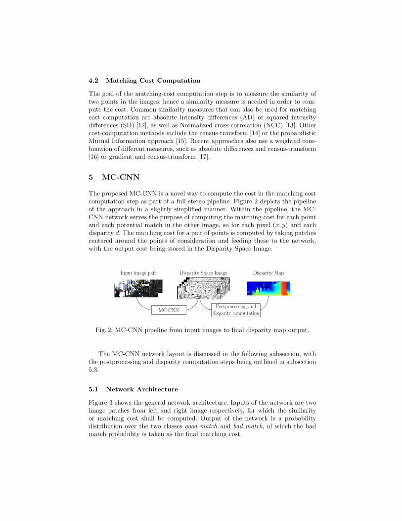
The proposed MC-CNN is a novel way to compute the cost in the matching costcomputation step as part of a full stereo pipeline. Figure 2 depicts the pipelineof the approach in a slightly simplified manner. Within the pipeline, the MC-CNN network serves the purpose of computing the matching cost for each pointand each potential match in the other image, so for each pixel (x, y) and eachdisparity d. The matching cost for a pair of points is computed by taking patchescentered around the points of consideration and feeding these to the network,with the output cost being stored in the Disparity Space Image.

Input image pair

MC-CNN

Disparity Space Image

Postprocessing and

disparity computation

Disparity Map

Fig. 2: MC-CNN pipeline from input images to final disparity map output.

The MC-CNN network layout is discussed in the following subsection, withthe postprocessing and disparity computation steps being outlined in subsection5.3.

5.1 Network Architecture

Figure 3 shows the general network architecture. Inputs of the network are twoimage patches from left and right image respectively, for which the similarityor matching cost shall be computed. Output of the network is a probabilitydistribution over the two classes good match and bad match, of which the badmatch probability is taken as the final matching cost.

Right

input patch

9

95

5

32

5

5

200 200

Left

input patch

9

95

5

32

5

5

200 200

feature concatenation400

300 300 300 300

2

Fig. 3: MC-CNN network architecture [3].

The network is divided into two major parts. The first stage up to the concate-nation layer makes up the feature extraction part, where features are extractedfrom the left and right patch. Each image patch is handled by an independentpath containing first a convolutional layer with two fully-connected layers follow-ing afterwards. It is important to note that the layer-weights in both paths aretied, meaning that the weights are the same in both paths, hence the identicalfeature extraction takes place in both paths, but for different input data.

After the feature-extraction part, the computed feature vectors are concate-nated to a combined feature-vector twice the size. This combined vector is thenpassed into the second network stage containing four fully-connected networklayers ending up in a softmax-classifier output layer. The second part is respon-sible for computing the similarity of the feature vectors of the individual patches.After all layers in the first and second stage, except for the softmax output, arectified linear activation function [18] is applied.

5.2 Network Training

As the used Convolutional Neural Network is a supervised machine learningtechnique, it is necessary to train the network before use. Ground-truth data toteach the network what comprises a good match versus a bad match is obtainedfrom recent stereo datasets such as the KITTI 2012 [19] dataset.

From the ground-truth disparities, positive and negative training examplesare generated, where each example consists of a pair of patches. Positive exam-ples are computed by taking patches at the true disparity and adding a slightrandom horizontal offset to increase robustness. Negative examples are obtainedsimilarly, but using a larger random offset such that the patches are still roughlyfrom the same area, but do not match directly anymore.

5.3 Post-processing and Disparity Computation

While the Disparity Space Image generated by the CNN could be used directlyto predict the disparity map by minimizing the cost along the disparity direc-tion in the DSI, a number of post-processing steps are applied in order to im-prove the results. All of these post-processing steps are state-of-the-art and are

not a particular contribution of the paper. The postprocessing pipeline is verymuch inspired by the approach presented by Mei et al. [16] including cross-basedcost-aggregation (CBCA) [20] and semi-global matching (SGM) [21]. Additionalchecks and refinements such as a left-right consistency check are also applied.

6 Results

An example for the disparity prediction obtained using the MC-CNN method isshown in figure 4. Figure 4b shows the resulting disparity map computed directlyfrom the DSI-output of the CNN. In this intermediate result, a large amount ofartifacts and mismatches is visible, especially in the overexposed areas on the left(street, building) due to low texture in these regions. Nevertheless the disparityestimate is already quite accurate in many areas.

(a) Left input image from dataset.

(b) Disparity map D(x, y) directly after CNN (without post-processing).

(c) Final disparity map D(x, y) after all post-processing.

Fig. 4: Disparity results for an example image pair from KITTI 2015 dataset [22].Results have been computed using the slightly revised MC-CNN-acrt journalarchitecture [23].

The final and improved result after all post-processing steps is depicted infigure 4c. The disparity estimate is heavily smoothed and practically all mis-matches have been removed, resulting in an excellent disparity estimate whereall foreground objects are clearly distinguishable.

Table 1: KITTI 2012 [19] benchmark results (Top 5) as of November 5, 2015

Rank Method Out-Noc Avg-Noc Runtime Environment

1 MC-CNN-acrt [23] 2.43 % 0.7 px 67 s Nvidia GTX Titan X2 Displets [24] 2.47 % 0.7 px 265 s >8 cores @ 3.0 Ghz3 MC-CNN [3] 2.61 % 0.8 px 100 s Nvidia GTX Titan4 PRSM [25] 2.78 % 0.7 px 300 s 1 core @ 2.5 Ghz5 SPS-StFl [26] 2.83 % 0.8 px 35 s 1 core @ 3.5 Ghz

In addition to the good subjective visual results, the method has been sub-mitted to a number of state-of-the-art stereo vision benchmarks and ranks verywell in them. As displayed in table 1, MC-CNN currently ranks third in theKITTI 2012 benchmark with an error of more than 3px in 2.65% of the pix-els in non-occluded areas. It is important to note that the second-best methodDisplets also uses the MC-CNN cost computation, but applies a specialized post-processing to increase the accuracy. Finally, the top-ranking method is currentlyMC-CNN-acrt, which is an improved journal version of MC-CNN by the sameauthors. At the time of writing, this method also ranks first in the KITTI 2015[22] and Middlebury 2014 [27] benchmarks.

7 Conclusions

The presented paper proposes an entirely new approach for matching cost com-putation in a stereo vision pipeline. It is the first method to take an existingstereo vision pipeline and replace one step thereof with a Convolutional NeuralNetwork. While the network achieves stunning results as-is, additional state-of-the-art pipeline steps are still needed as post-processing steps in order toachieve competitive results. Including this post-processing, the method achievestop-results in all recent major stereo vision benchmark suites.

One of largest disadvantages of the proposed method is the fairly high com-putational effort required to compute the cost, taking up to minutes on recenthigh-end GPUs. This issue has already been addressed in a revised journal ver-sion of the presented paper, which features an improved feature extraction andan additional fast network variant that reduces the computation time to therange of seconds while achieving almost the same accuracy.

Despite the great success in current benchmarks, there are various oppor-tunities to increase the accuracy even further. An approach could be to usemulti-scale CNNs [28] to incorporate more global information into the cost com-putation. As also suggested by the authors, using larger training sets might bebeneficial. This could be done by using synthetically generated ground-truth datain order to pre-train the network first and subsequently fine-tune the weights onreal-world training data.

References

1. Barnard, S.T., Fischler, M.A.: Computational stereo. ACM Comput. Surv. 14(4)(December 1982) 553–572

2. Scharstein, D., Szeliski, R., Zabih, R.: A taxonomy and evaluation of dense two-frame stereo correspondence algorithms. In: Stereo and Multi-Baseline Vision,2001. (SMBV 2001). Proceedings. IEEE Workshop on. (2001) 131–140

3. Zbontar, J., LeCun, Y.: Computing the stereo matching cost with a convolutionalneural network. In: The IEEE Conference on Computer Vision and Pattern Recog-nition (CVPR). (June 2015)

4. Hartley, R., Zisserman, A.: Multiple View Geometry in Computer Vision. Secondedn. Cambridge University Press (2003)

5. Loop, C., Zhang, Z.: Computing rectifying homographies for stereo vision. In:Computer Vision and Pattern Recognition, 1999. IEEE Computer Society Confer-ence on. Volume 1. (1999) 131 Vol. 1

6. LeCun, Y., Boser, B., Denker, J.S., Henderson, D., Howard, R.E., Hubbard, W.,Jackel, L.D.: Backpropagation applied to handwritten zip code recognition. NeuralComput. 1(4) (December 1989) 541–551

7. Lecun, Y., Bottou, L., Bengio, Y., Haffner, P.: Gradient-based learning applied todocument recognition. In: Proceedings of the IEEE. (1998) 2278–2324

8. Krizhevsky, A., Sutskever, I., Hinton, G.E.: Imagenet classification with deep con-volutional neural networks. In Pereira, F., Burges, C., Bottou, L., Weinberger, K.,eds.: Advances in Neural Information Processing Systems 25. Curran Associates,Inc. (2012) 1097–1105

9. Long, J., Shelhamer, E., Darrell, T.: Fully convolutional networks for semanticsegmentation. CVPR (to appear) (November 2015)

10. Fischer, P., Dosovitskiy, A., Ilg, E., Hausser, P., Hazırbas, C., Golkov, V., van derSmagt, P., Cremers, D., Brox, T.: FlowNet: Learning Optical Flow with Convolu-tional Networks. In: IEEE International Conference on Computer Vision (ICCV).(December 2015)

11. Intille, S., Bobick, A.: Disparity-space images and large occlusion stereo. In Ek-lundh, J.O., ed.: Computer Vision — ECCV ’94. Volume 801 of Lecture Notes inComputer Science. Springer Berlin Heidelberg (1994) 179–186

12. Hirschmuller, H., Scharstein, D.: Evaluation of cost functions for stereo matching.In: Computer Vision and Pattern Recognition, 2007. CVPR ’07. IEEE Conferenceon. (June 2007) 1–8

13. Sinha, S.N., Scharstein, D., Szeliski, R.: Efficient high-resolution stereo matchingusing local plane sweeps. In: Proceedings of the 2014 IEEE Conference on Com-puter Vision and Pattern Recognition. CVPR ’14, Washington, DC, USA, IEEEComputer Society (2014) 1582–1589

14. Zabih, R., Woodfill, J.: Non-parametric local transforms for computing visualcorrespondence. In Eklundh, J.O., ed.: Computer Vision — ECCV ’94. Volume801 of Lecture Notes in Computer Science. Springer Berlin Heidelberg (1994)151–158

15. Kim, J., Kolmogorov, V., Zabih, R.: Visual correspondence using energy mini-mization and mutual information. In: Computer Vision, 2003. Proceedings. NinthIEEE International Conference on. (Oct 2003) 1033–1040 vol.2

16. Mei, X., Sun, X., Zhou, M., shaohui Jiao, Wang, H., Zhang, X.: On building an ac-curate stereo matching system on graphics hardware. In: Computer Vision Work-shops (ICCV Workshops), 2011 IEEE International Conference on. (Nov 2011)467–474

17. Zhang, C., Li, Z., Cheng, Y., Cai, R., Chao, H., Rui, Y.: Meshstereo: A globalstereo model with mesh alignment regularization for view interpolation. In: IEEEInternational Conference on Computer Vision (ICCV). (2015)

18. Nair, V., Hinton, G.E.: Rectified linear units improve restricted boltzmann ma-chines. In Furnkranz, J., Joachims, T., eds.: Proceedings of the 27th InternationalConference on Machine Learning (ICML-10), Omnipress (2010) 807–814

19. Geiger, A., Lenz, P., Urtasun, R.: Are we ready for autonomous driving? thekitti vision benchmark suite. In: Conference on Computer Vision and PatternRecognition (CVPR). (2012)

20. Zhang, K., Lu, J., Lafruit, G.: Cross-based local stereo matching using orthogonalintegral images. Circuits and Systems for Video Technology, IEEE Transactionson 19(7) (July 2009) 1073–1079

21. Hirschmuller, H.: Stereo processing by semiglobal matching and mutual informa-tion. Pattern Analysis and Machine Intelligence, IEEE Transactions on 30(2) (Feb2008) 328–341

22. Menze, M., Geiger, A.: Object scene flow for autonomous vehicles. In: Conferenceon Computer Vision and Pattern Recognition (CVPR). (2015)

23. Zbontar, J., LeCun, Y.: Stereo matching by training a convolutional neural networkto compare image patches. arXiv preprint arXiv:1510.05970 (2015)

24. Guney, F., Geiger, A.: Displets: Resolving stereo ambiguities using object knowl-edge. In: Proceedings of the IEEE Conference on Computer Vision and PatternRecognition. (2015) 4165–4175

25. Vogel, C., Schindler, K., Roth, S.: 3d scene flow estimation with a piecewise rigidscene model. International Journal of Computer Vision (2015) 1–28

26. Yamaguchi, K., McAllester, D., Urtasun, R.: Efficient joint segmentation, occlusionlabeling, stereo and flow estimation. In Fleet, D., Pajdla, T., Schiele, B., Tuyte-laars, T., eds.: Computer Vision – ECCV 2014. Volume 8693 of Lecture Notes inComputer Science. Springer International Publishing (2014) 756–771

27. Scharstein, D., Hirschmuller, H., Kitajima, Y., Krathwohl, G., Nesic, N., Wang,X., Westling, P.: High-resolution stereo datasets with subpixel-accurate groundtruth. In: 36th German Conference on Pattern Recognition (GCPR). (September2014)

28. Eigen, D., Puhrsch, C., Fergus, R.: Depth map prediction from a single imageusing a multi-scale deep network. CoRR abs/1406.2283 (2014)