University of Groningen

Efficient binocular stereo correspondence matching with 1-D Max-TreesBrandt, Rafaël; Strisciuglio, Nicola; Petkov, Nicolai; Wilkinson, Michael H. F.

Published in:Pattern Recognition Letters

DOI:10.1016/j.patrec.2020.02.019

IMPORTANT NOTE: You are advised to consult the publisher's version (publisher's PDF) if you wish to cite fromit. Please check the document version below.

Document VersionPublisher's PDF, also known as Version of record

Publication date:2020

Link to publication in University of Groningen/UMCG research database

Citation for published version (APA):Brandt, R., Strisciuglio, N., Petkov, N., & Wilkinson, M. H. F. (2020). Efficient binocular stereocorrespondence matching with 1-D Max-Trees. Pattern Recognition Letters, 135, 402-408.https://doi.org/10.1016/j.patrec.2020.02.019

CopyrightOther than for strictly personal use, it is not permitted to download or to forward/distribute the text or part of it without the consent of theauthor(s) and/or copyright holder(s), unless the work is under an open content license (like Creative Commons).

The publication may also be distributed here under the terms of Article 25fa of the Dutch Copyright Act, indicated by the “Taverne” license.More information can be found on the University of Groningen website: https://www.rug.nl/library/open-access/self-archiving-pure/taverne-amendment.

Take-down policyIf you believe that this document breaches copyright please contact us providing details, and we will remove access to the work immediatelyand investigate your claim.

Downloaded from the University of Groningen/UMCG research database (Pure): http://www.rug.nl/research/portal. For technical reasons thenumber of authors shown on this cover page is limited to 10 maximum.

Download date: 15-03-2022

Pattern Recognition Letters 135 (2020) 402–408

Contents lists available at ScienceDirect

Pattern Recognition Letters

journal homepage: www.elsevier.com/locate/patrec

Efficient binocular stereo correspondence matching with 1-D

Max-Trees

Rafaël Brandt, Nicola Strisciuglio, Nicolai Petkov, Michael H.F. Wilkinson

∗

Bernoulli Institute, University of Groningen, P.O. Box 407, AK Groningen 9700, the Netherlands

a r t i c l e i n f o

Article history:

Received 14 June 2019

Revised 4 December 2019

Accepted 19 February 2020

Available online 20 February 2020

MSC:

41A05

41A10

65D05

65D17

Keywords:

Stereo matching

Mathematical morphology

Tree structures

a b s t r a c t

Extraction of depth from images is of great importance for various computer vision applications. Meth-

ods based on convolutional neural networks are very accurate but have high computation requirements,

which can be achieved with GPUs. However, GPUs are difficult to use on devices with low power require-

ments like robots and embedded systems. In this light, we propose a stereo matching method appropri-

ate for applications in which limited computational and energy resources are available. The algorithm is

based on a hierarchical representation of image pairs which is used to restrict disparity search range.

We propose a cost function that takes into account region contextual information and a cost aggregation

method that preserves disparity borders. We tested the proposed method on the Middlebury and KITTI

benchmark data sets and on the TrimBot2020 synthetic data. We achieved accuracy and time efficiency

results that show that the method is suitable to be deployed on embedded and robotics systems.

© 2020 The Authors. Published by Elsevier B.V.

This is an open access article under the CC BY-NC-ND license.

( http://creativecommons.org/licenses/by-nc-nd/4.0/ )

p

i

m

a

i

d

i

p

i

a

t

p

s

l

h

[

i

n

m

p

p

1. Introduction

Extraction of depth from images is of great importance for com-

puter vision applications, such as autonomous car driving [19] , ob-

stacle avoidance for robots [16] , 3D reconstruction [24] , Simultane-

ous Localization and Mapping [5] , among others. Given a pair of

rectified images recorded by calibrated cameras, a typical pipeline

for binocular stereo matching exploits epipolar geometry to find

corresponding pixels between the left and right image and create

a map of their horizontal displacement, i.e. a disparity map. For a

pixel ( x , y ) in the left image, its corresponding pixel (x − d, y ) is

searched for in the right image and a matching cost is associated

with it. If a corresponding pixel is found, the perceived depth is

computed as Bf / d where B is the baseline, f the camera focal length

and d is the measured disparity. The match with the lowest cost is

used to select the best disparity value and construct the disparity

map.

In the literature, various approaches to compute the matching

cost have been proposed. The similarity between two pixels has of-

ten been expressed as their absolute image gradient or gray-level

difference [23] . In regions with repeating patterns or without tex-

ture, the matching cost of a pixel can be very low at multiple dis-

∗ Corresponding author.

E-mail address: m.h.f.wilkinson@rug.nl (M.H.F. Wilkinson).

a

i

p

A

https://doi.org/10.1016/j.patrec.2020.02.019

0167-8655/© 2020 The Authors. Published by Elsevier B.V. This is an open access article u

arities. To reduce such ambiguity, the similarity of the surround-

ng region of the concerned pixels can be measured instead. The

atching cost of a pixel pair is computed as the (weighted) aver-

ge of the matching cost of corresponding pixels in the surround-

ng regions. Therefore, the disparity predictions near disparity bor-

ers are unreliable when surrounding pixels with different dispar-

ty than the considered pixel pair have a non-zero weight [17] . Dis-

arity borders have been estimated, for instance, using color sim-

larity and proximity to weigh the contribution of a pixel to an

verage of another pixel by Yoon and Kweon [33] . A scheme which

akes into account the strength of image boundaries in between

ixels has been proposed by Chen et al. [1] . Zhang et al. [35] con-

tructed horizontal and vertical line segments based on color simi-

arity and spatial distance of pixels, and costs were aggregated over

orizontal and then over vertical line segments.

The creation of large stereo data-sets with ground-truths

22] has facilitated the development of methods that learn a sim-

larity measure between (two) image patches using convolutional

eural networks (CNNs). One of the first CNN stereo matching

ethods, based on a siamese network architecture, has been pro-

osed by Zbontar et al. [34] . An efficient variation has been pro-

osed by Luo et al. [11] that formulated the disparity computation

s a multi-class problem, in which each class is a possible dispar-

ty value. These two approaches are restricted to small patch in-

uts. Using larger patches may produce blurred boundaries [17] .

pproaches to increase the receptive field while keeping details

nder the CC BY-NC-ND license. ( http://creativecommons.org/licenses/by-nc-nd/4.0/ )

R. Brandt, N. Strisciuglio and N. Petkov et al. / Pattern Recognition Letters 135 (2020) 402–408 403

h

w

A

c

m

e

c

p

n

p

[

i

s

i

v

r

b

[

t

a

r

M

b

b

r

c

p

a

i

a

c

a

w

i

[

t

a

t

b

o

e

p

2

3

a

2

o

l

t

s

a

t

r

m

2

s

n

a

r

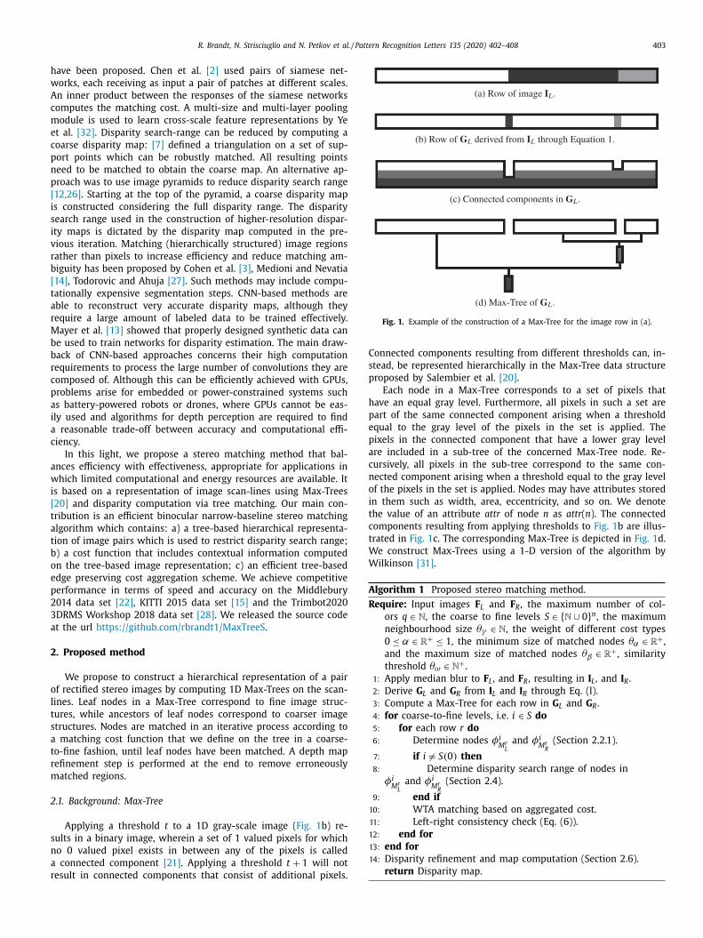
Fig. 1. Example of the construction of a Max-Tree for the image row in (a).

C

s

p

h

p

e

p

a

c

n

o

i

t

c

t

W

W

A

R

ave been proposed. Chen et al. [2] used pairs of siamese net-

orks, each receiving as input a pair of patches at different scales.

n inner product between the responses of the siamese networks

omputes the matching cost. A multi-size and multi-layer pooling

odule is used to learn cross-scale feature representations by Ye

t al. [32] . Disparity search-range can be reduced by computing a

oarse disparity map: [7] defined a triangulation on a set of sup-

ort points which can be robustly matched. All resulting points

eed to be matched to obtain the coarse map. An alternative ap-

roach was to use image pyramids to reduce disparity search range

12,26] . Starting at the top of the pyramid, a coarse disparity map

s constructed considering the full disparity range. The disparity

earch range used in the construction of higher-resolution dispar-

ty maps is dictated by the disparity map computed in the pre-

ious iteration. Matching (hierarchically structured) image regions

ather than pixels to increase efficiency and reduce matching am-

iguity has been proposed by Cohen et al. [3] , Medioni and Nevatia

14] , Todorovic and Ahuja [27] . Such methods may include compu-

ationally expensive segmentation steps. CNN-based methods are

ble to reconstruct very accurate disparity maps, although they

equire a large amount of labeled data to be trained effectively.

ayer et al. [13] showed that properly designed synthetic data can

e used to train networks for disparity estimation. The main draw-

ack of CNN-based approaches concerns their high computation

equirements to process the large number of convolutions they are

omposed of. Although this can be efficiently achieved with GPUs,

roblems arise for embedded or power-constrained systems such

s battery-powered robots or drones, where GPUs cannot be eas-

ly used and algorithms for depth perception are required to find

reasonable trade-off between accuracy and computational effi-

iency.

In this light, we propose a stereo matching method that bal-

nces efficiency with effectiveness, appropriate for applications in

hich limited computational and energy resources are available. It

s based on a representation of image scan-lines using Max-Trees

20] and disparity computation via tree matching. Our main con-

ribution is an efficient binocular narrow-baseline stereo matching

lgorithm which contains: a) a tree-based hierarchical representa-

ion of image pairs which is used to restrict disparity search range;

) a cost function that includes contextual information computed

n the tree-based image representation; c) an efficient tree-based

dge preserving cost aggregation scheme. We achieve competitive

erformance in terms of speed and accuracy on the Middlebury

014 data set [22] , KITTI 2015 data set [15] and the Trimbot2020

DRMS Workshop 2018 data set [28] . We released the source code

t the url https://github.com/rbrandt1/MaxTreeS .

. Proposed method

We propose to construct a hierarchical representation of a pair

f rectified stereo images by computing 1D Max-Trees on the scan-

ines. Leaf nodes in a Max-Tree correspond to fine image struc-

ures, while ancestors of leaf nodes correspond to coarser image

tructures. Nodes are matched in an iterative process according to

matching cost function that we define on the tree in a coarse-

o-fine fashion, until leaf nodes have been matched. A depth map

efinement step is performed at the end to remove erroneously

atched regions.

.1. Background: Max-Tree

Applying a threshold t to a 1D gray-scale image ( Fig. 1 b) re-

ults in a binary image, wherein a set of 1 valued pixels for which

o 0 valued pixel exists in between any of the pixels is called

connected component [21] . Applying a threshold t + 1 will not

esult in connected components that consist of additional pixels.

onnected components resulting from different thresholds can, in-

tead, be represented hierarchically in the Max-Tree data structure

roposed by Salembier et al. [20] .

Each node in a Max-Tree corresponds to a set of pixels that

ave an equal gray level. Furthermore, all pixels in such a set are

art of the same connected component arising when a threshold

qual to the gray level of the pixels in the set is applied. The

ixels in the connected component that have a lower gray level

re included in a sub-tree of the concerned Max-Tree node. Re-

ursively, all pixels in the sub-tree correspond to the same con-

ected component arising when a threshold equal to the gray level

f the pixels in the set is applied. Nodes may have attributes stored

n them such as width, area, eccentricity, and so on. We denote

he value of an attribute attr of node n as attr ( n ). The connected

omponents resulting from applying thresholds to Fig. 1 b are illus-

rated in Fig. 1 c. The corresponding Max-Tree is depicted in Fig. 1 d.

e construct Max-Trees using a 1-D version of the algorithm by

ilkinson [31] .

lgorithm 1 Proposed stereo matching method.

equire: Input images F L and F R , the maximum number of col-

ors q ∈ N , the coarse to fine levels S ∈ { N ∪ 0 } n , the maximum

neighbourhood size θγ ∈ N , the weight of different cost types

0 ≤ α ∈ R

+ ≤ 1 , the minimum size of matched nodes θα ∈ R

+ ,and the maximum size of matched nodes θβ ∈ R

+ , similarity

threshold θω ∈ N

+ . 1: Apply median blur to F L , and F R , resulting in I L , and I R .

2: Derive G L and G R from I L and I R through Eq. (l).

3: Compute a Max-Tree for each row in G L and G R .

4: for coarse-to-fine levels, i.e. i ∈ S do

5: for each row r do

6: Determine nodes φi M

r L

and φi M

r R

(Section 2.2.1).

7: if i � = S(0) then

8: Determine disparity search range of nodes in

φi M

r L

and φi M

r R

(Section 2.4).

9: end if

10: WTA matching based on aggregated cost.

11: Left-right consistency check (Eq. (6)).

12: end for

13: end for

14: Disparity refinement and map computation (Section 2.6).

return Disparity map.

404 R. Brandt, N. Strisciuglio and N. Petkov et al. / Pattern Recognition Letters 135 (2020) 402–408

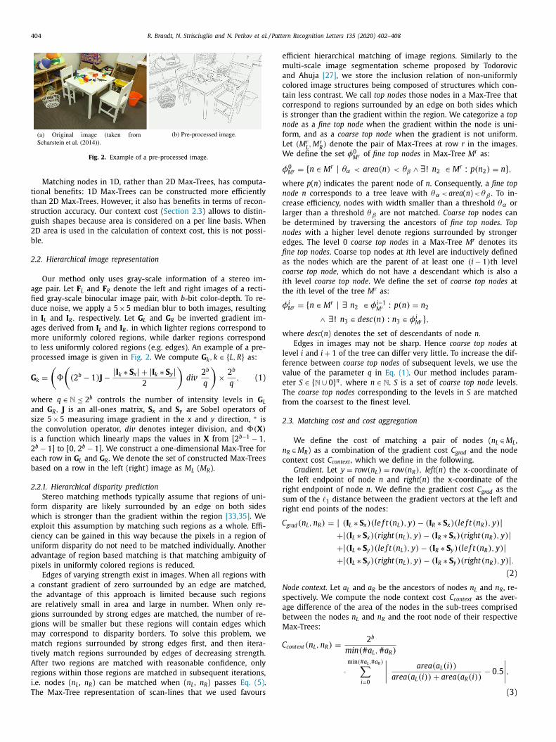
Fig. 2. Example of a pre-processed image.

e

m

a

c

t

c

i

n

f

L

W

φ

w

n

c

l

b

n

e

fi

a

c

i

t

φ

w

l

f

v

e

T

f

2

n

c

t

r

s

r

C

N

s

a

b

M

C

Matching nodes in 1D, rather than 2D Max-Trees, has computa-

tional benefits: 1D Max-Trees can be constructed more efficiently

than 2D Max-Trees. However, it also has benefits in terms of recon-

struction accuracy. Our context cost ( Section 2.3 ) allows to distin-

guish shapes because area is considered on a per line basis. When

2D area is used in the calculation of context cost, this is not possi-

ble.

2.2. Hierarchical image representation

Our method only uses gray-scale information of a stereo im-

age pair. Let F L and F R denote the left and right images of a recti-

fied gray-scale binocular image pair, with b -bit color-depth. To re-

duce noise, we apply a 5 × 5 median blur to both images, resulting

in I L and I R , respectively. Let G L and G R be inverted gradient im-

ages derived from I L and I R , in which lighter regions correspond to

more uniformly colored regions, while darker regions correspond

to less uniformly colored regions (e.g. edges). An example of a pre-

processed image is given in Fig. 2 . We compute G k , k ∈ { L, R } as:

G k =

(�

((2

b − 1) J − | I k ∗ S x | + | I k ∗ S y | 2

)di v

2

b

q

)× 2

b

q , (1)

where q ∈ N ≤ 2 b controls the number of intensity levels in G L

and G R , J is an all-ones matrix, S x and S y are Sobel operators of

size 5 × 5 measuring image gradient in the x and y direction, ∗ is

the convolution operator, di v denotes integer division, and �( X )

is a function which linearly maps the values in X from [ 2 b−1 − 1 ,

2 b − 1 ] to [0, 2 b − 1 ]. We construct a one-dimensional Max-Tree for

each row in G L and G R . We denote the set of constructed Max-Trees

based on a row in the left (right) image as M L ( M R ).

2.2.1. Hierarchical disparity prediction

Stereo matching methods typically assume that regions of uni-

form disparity are likely surrounded by an edge on both sides

which is stronger than the gradient within the region [33,35] . We

exploit this assumption by matching such regions as a whole. Effi-

ciency can be gained in this way because the pixels in a region of

uniform disparity do not need to be matched individually. Another

advantage of region based matching is that matching ambiguity of

pixels in uniformly colored regions is reduced.

Edges of varying strength exist in images. When all regions with

a constant gradient of zero surrounded by an edge are matched,

the advantage of this approach is limited because such regions

are relatively small in area and large in number. When only re-

gions surrounded by strong edges are matched, the number of re-

gions will be smaller but these regions will contain edges which

may correspond to disparity borders. To solve this problem, we

match regions surrounded by strong edges first, and then itera-

tively match regions surrounded by edges of decreasing strength.

After two regions are matched with reasonable confidence, only

regions within those regions are matched in subsequent iterations,

i.e. nodes ( n L , n R ) can be matched when ( n L , n R ) passes Eq. (5) .

The Max-Tree representation of scan-lines that we used favours

fficient hierarchical matching of image regions. Similarly to the

ulti-scale image segmentation scheme proposed by Todorovic

nd Ahuja [27] , we store the inclusion relation of non-uniformly

olored image structures being composed of structures which con-

ain less contrast. We call top nodes those nodes in a Max-Tree that

orrespond to regions surrounded by an edge on both sides which

s stronger than the gradient within the region. We categorize a top

ode as a fine top node when the gradient within the node is uni-

orm, and as a coarse top node when the gradient is not uniform.

et (M

r L , M

r R ) denote the pair of Max-Trees at row r in the images.

e define the set φ0 M

r of fine top nodes in Max-Tree M

r as:

0 M

r = { n ∈ M

r | θα < area (n ) < θβ ∧ ∃ ! n 2 ∈ M

r : p(n 2 ) = n } , here p ( n ) indicates the parent node of n . Consequently, a fine top

ode n corresponds to a tree leave with θα < area ( n ) < θβ . To in-

rease efficiency, nodes with width smaller than a threshold θα or

arger than a threshold θβ are not matched. Coarse top nodes can

e determined by traversing the ancestors of fine top nodes . Top

odes with a higher level denote regions surrounded by stronger

dges. The level 0 coarse top nodes in a Max-Tree M

r denotes its

ne top nodes . Coarse top nodes at i th level are inductively defined

s the nodes which are the parent of at least one (i − 1) th level

oarse top node , which do not have a descendant which is also a

th level coarse top node . We define the set of coarse top nodes at

he i th level of the tree M

r as:

i M

r = { n ∈ M

r | ∃ n 2 ∈ φi −1 M

r : p(n ) = n 2

∧ ∃ ! n 3 ∈ desc(n ) : n 3 ∈ φi M

r } , here desc ( n ) denotes the set of descendants of node n .

Edges in images may not be sharp. Hence coarse top nodes at

evel i and i + 1 of the tree can differ very little. To increase the dif-

erence between coarse top nodes of subsequent levels, we use the

alue of the parameter q in Eq. (1) . Our method includes param-

ter S ∈ { N ∪ 0 } n , where n ∈ N . S is a set of coarse top node levels.

he coarse top nodes corresponding to the levels in S are matched

rom the coarsest to the finest level.

.3. Matching cost and cost aggregation

We define the cost of matching a pair of nodes ( n L ∈ M L ,

R ∈ M R ) as a combination of the gradient cost C grad and the node

ontext cost C context , which we define in the following.

Gradient. Let y = row (n L ) = row (n R ) , left ( n ) the x-coordinate of

he left endpoint of node n and right ( n ) the x-coordinate of the

ight endpoint of node n . We define the gradient cost C grad as the

um of the 1 distance between the gradient vectors at the left and

ight end points of the nodes:

grad (n L , n R ) = | ( I L ∗ S x )(le f t(n L ) , y ) − ( I R ∗ S x )(le f t(n R ) , y ) | + | ( I L ∗ S x )(right(n L ) , y ) − ( I R ∗ S x )(right(n R ) , y ) | + | ( I L ∗ S y )(le f t(n L ) , y ) − ( I R ∗ S y )(le f t(n R ) , y ) | + | ( I L ∗ S y )(right(n L ) , y ) − ( I R ∗ S y )(right(n R ) , y ) | .

(2)

ode context. Let a L and a R be the ancestors of nodes n L and n R , re-

pectively. We compute the node context cost C context as the aver-

ge difference of the area of the nodes in the sub-trees comprised

etween the nodes n L and n R and the root node of their respective

ax-Trees:

context (n L , n R ) =

2

b

min (# a L , # a R )

·min (# a L , # a R ) ∑

i =0

∣∣∣∣ area (a L (i ))

area (a L (i )) + area (a R (i )) − 0 . 5

∣∣∣∣, (3)

R. Brandt, N. Strisciuglio and N. Petkov et al. / Pattern Recognition Letters 135 (2020) 402–408 405

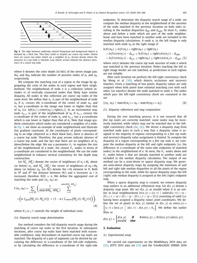
Fig. 3. The edge between uniformly colored foreground and background objects is

denoted by a thick line. Thin lines (solid or striped) are coarse top nodes. Dotted

lines are coarse top nodes which are a neighbor of n 0 . Arrows denote where the

presence of a top node is checked. Gray (black) arrows indicate the absence (pres-

ence) of a coarse top node.

w

#

r

g

b

c

d

s

n

n

o

n

x

w

d

I

t

i

a

a

a

o

y

n

c

(

a

i

i

m

C

w

2

m

i

a

m

c

o

e

c

o

s

a

h

m

m

l

w

w

r

a

b

m

a

o

w

s

{2

fi

r

r

m

s

a

d

p

d

n

θ

i

m

a

l

c

(

o

m

d

l

2

h

fi {

fi

d

3

3

[

here b denotes the color depth (in bits) of the stereo image pair,

a L and # a R indicate the number of ancestor nodes of n L and n R ,

espectively.

We compute the matching cost of a region in the image by ag-

regating the costs of the nodes in such region and their neigh-

orhood. The neighborhood of node n is a collection (which in-

ludes n ) of vertically connected nodes that likely have similar

isparity. All nodes in this collection are coarse top nodes of the

ame level. We define that n 1 is part of the neighborhood of node

0 if n 1 crosses the x-coordinate of the center of node n 0 , and

1 has y-coordinate in the image one lower or higher than that

f n 0 (i.e. left ( n 1 ) ≤ center ( n 0 ) ≤ right ( n 1 )). In an incremental way,

ode n j+1 is part of the neighborhood of n 0 if n j+1 crosses the

-coordinate of the center of node n j , and n j+1 has a y-coordinate

hich is one lower or higher than that of n j . Note that image gra-

ient constraints which nodes are considered a neighbor of a node.

n Fig. 3 , we show an example of node neighborhood and illustrate

his gradient constraint. At the coordinates of pixels correspond-

ng to an edge (depicted as a thick black line), there is absence of

coarse top node. Therefore, the gray arrows indicate absence of

coarse top node, and the fact that there are no neighbors of n 0 bove/below the edge. We use a parameter θγ to regulate the size

f the neighborhood of a node: the closest θγ nodes in terms of

-coordinate are considered in the neighborhood. We use the node

eighborhood to enhance vertical consistency for the depth map

onstruction.

Let N

T n L

( N

B n L

) denote the vector of neighbours of n L ∈ M L above

or below) n L , and N

T n R

( N

B n R

) the vector of neighbours of n R ∈ M R

bove (or below) n R . Let N ( i ) denote the i -th element in N . Both

n N

B and N

T the distance between N ( i ) and n increases as i is

ncreased, therefore N (0) = n . We define the aggregated cost of

atching the node pair ( n L , n R ) as:

(n L , n R ) =

∑

s = { T,B }

(1

min (# N

s n L

, # N

s n R

)

min (# N s n L , # N s n R

) ∑

i =0

×(α C grad

(N

s n L

(i ) , N

s n R

(i ) )

+ (1 − α) C context

(N

s n L

(i ) , N

s n R

(i ) )))

,

(4)

here 0 ≤α ≤ 1 controls the weight of individual costs.

.4. Disparity search range determination

Our method considers the full disparity search range during the

atching of coarse top nodes in the first iteration. In subsequent

terations, after coarse top nodes have been matched with reason-

ble confidence, only descendants of matched coarse top nodes are

atched. The disparity of a pair of segments can be derived by cal-

ulating the difference in x-coordinate of the left-side endpoints,

r by calculating the difference in x-coordinate of the right-side

ndpoints. To determine the disparity search range of a node, we

ompute the median disparity in the neighborhood of the ancestor

f the node matched in the previous iteration on both sides re-

ulting in the median disparities d left and d right . At most θγ nodes

bove and below a node which are part of the node neighbor-

ood, and have been matched to another node are included in the

edian disparity calculations. A node n L in the left image is only

atched with node n R in the right image if:

e f t(n R ) ≤ le f t(n L ) ∧ right(n R ) ≤ right(n L )

∧ le f t (ct n (n L )) − d le f t ≤ le f t(n R ) ≤ right (ct n (n L )) − d right

∧ le f t (ct n (n L )) − d le f t ≤ right(n R ) ≤ right (ct n (n L )) − d right , (5)

here ctn ( n ) denotes the coarse top node ancestor of node n which

as matched in the previous iteration. Nodes touching the left or

ight image border are not matched, as predictions in such regions

re not reliable.

After each iteration we perform the left-right consistency check

y Weng et al. [30] , which detects occlusions and incorrect

atches. Given a matching of two pixels, disparity values are only

ssigned when both pixels have minimal matching cost with each

ther. Let match ( n ) denote the node matched to node n . The nodes

hich pass the left-right consistency check are contained in the

et:

(n L , n R ) | match (n L ) = n R ∧ match (n R ) = n L } . (6)

.5. Disparity refinement and map computation

During the tree matching process, it is not ensured that all

ne top nodes are correctly matched: some nodes may be incor-

ectly matched, while others may not be matched due to the left-

ight consistency check ( Eq. (6) ). We derive a disparity map from

atched node pairs in such a way that a disparity value is as-

igned in the majority of regions corresponding to a fine top node ,

nd incorrect disparity value assignment is limited. To compute the

isparity of a region corresponding to a fine top node n , we com-

ute the median disparity at the left and right endpoints (i.e. the

ifference in x-coordinate of the same-side endpoints of matched

odes) in the neighborhood of n . At most, the θγ nodes above and

γ nodes below n that are already matched to another node are

ncluded in the median disparity calculation. The output of our

ethod can be a semi-dense or sparse disparity map. We gener-

te semi-dense disparity maps by assigning the minimum of said

eft and right side median disparities to all the pixels of the region

orresponding to the node, while for sparse disparity maps the left

right) side median disparity is assigned at the left (right) endpoint

nly.

When a sparse disparity map is created, we remove disparity

ap outliers in an additional refinement step. Let d ( x , y ) denote a

isparity map pixel. We set d ( x , y ) as invalid when it is an out-

ier in local neighbourhood ln (x, y ) = { (c, r) | v alid (d (c, r)) ∧ (x −1) ≤ c < (x + 21) ∧ (y − 21) ≤ r < (y + 21) } consisting of valid (i.e.

aving been assigned a disparity value) pixel coordinates. We de-

ne the set of pixels in ln ( x , y ) similar to d ( x , y ) as sim (x, y ) =

(c, r) ∈ ln (x, y )

∣∣∣ | d(c, r) − d(x, y ) | ≤ θω

}

. We define the outlier

lter as

(x, y ) =

{d(x, y ) if # sim (x, y ) ≥ #(ln (x, y ) \ sim (x, y )) in v alid else

.

. Evaluation

.1. Experimental setup

We carried out experiments on the Middlebury 2014 data set

22] , KITTI 2015 data set [15] and the TrimBot2020 3DRMS 2018

406 R. Brandt, N. Strisciuglio and N. Petkov et al. / Pattern Recognition Letters 135 (2020) 402–408

o

2

t

S

K

b

3

s

t

t

s

d

t

i

g

p

s

F

a

a

r

w

r

b

e

w

t

data set of synthetic garden images [28] . We evaluate the perfor-

mance of our algorithm in terms of computational efficiency and

accuracy of computed disparity maps.

The Middlebury training data set contains 15 high resolution

natural stereo pairs of indoor scenes and ground truth disparity

maps. The KITTI 2015 training data set contains 200 natural stereo

pairs of outdoor road scenes and ground truth disparity maps.

The Trimbot2020 training data set contains 5 × 4 sets of 100 low-

resolution synthetic stereo pairs of outdoor garden scenes with

ground truth depth maps. They were rendered from 3D synthetic

models of gardens, with different illumination and weather condi-

tions (i.e. clear, cloudy, overcast, sunset and twilight), in the con-

text of the TrimBot2020 project [25] . The (vcam_0, vcam_1) stereo

pairs of the Trimbot2020 training data set were used for evalua-

tion.

For the Middlebury and KITTI data sets, we compute the aver-

age absolute error in pixels (avgerr) with respect to ground truth

disparity maps. Only non-occluded pixels which were assigned a

disparity value (i.e. have both been assigned a disparity value by

the evaluated method and contain a disparity value in the ground

truth) are considered. For the Trimbot2020 data set, we compute

the average absolute error in meters (avgerr m

) with respect to

ground truth depth maps. Only pixels which were assigned a depth

value (i.e. have been assigned a depth value by our method and

contain a non-zero depth value in the ground truth) are consid-

ered. Furthermore, we measure the algorithm processing time in

seconds normalized by the number of megapixels (sec/MP) in the

input image. We do not resize the original images in the datasets.

For all data sets, we compute the average density (i.e. percentage

of pixels with a disparity estimation w.r.t. total number of image

pixels) of the disparity maps computed by the considered meth-

o

Fig. 4. Example images from the Middlebury (a), TrimBot2020 (e), and KITTI 2015 (i,m) d

semi-dense results are shown in (c,g,k,o) and (d,h,lp), respectively. Morphological dilation

ds (d%). We performed the experiments on an Intel® Core TM i7-

600K CPU running at 3.40GHz with 8GB DDR3 memory. For all

he experiments we set the value of the parameters as q = 5 ,

= { 1 , 0 } , θγ = 6 , α = 0 . 8 , θα = 3, θω = 3 . For the Middlebury and

ITTI data sets, θβ is 1/3 of the input image width. For the Trim-

ot2020 data set, θβ is 1/15 of the input image width.

.2. Results and comparison

In Fig. 4 , we show example images from the Middlebury (a),

ynthetic TrimBot2020 (e), and KITTI (i,m) data sets, together with

heir ground truth depth images ((b), (f) and (j,n), respectively). In

he third column of Fig. 4 , we show the output of our sparse recon-

truction approach, while in the fourth column that of the semi-

ense reconstruction algorithm. Our semi-dense method makes

he assumption that regions with little texture are flat because

nformation can not be extracted from a uniformly colored re-

ion which allows to recover its disparity. We observed that the

roposed method estimates disparity in texture-less regions with

atisfying robustness (e.g. the table top and the chair surface in

ig. 4 d). When semi-dense reconstruction is applied, in the case of

n object containing a hole, the foreground disparity is sometimes

ssigned to the background when the background is a texture-less

egion. This is seen in the semi-dense output shown in Fig. 4 h. In

hat way our method behaves when faced with uniformly colored

egions can be altered through parameter θβ . Due to inherent am-

iguity, this parameter should be set based on high level knowl-

dge about the dataset. A dataset containing more (less) objects

ith a hole that are in front of a uniformly colored background

han objects that do not contain a hole but have a uniformly col-

red region on their surface should use a smaller (larger) θβ value.

ata sets, with corresponding (b,f,j,n) ground truth disparity images. The sparse and

was applied to disparity map estimates for visualization purposes only.

R. Brandt, N. Strisciuglio and N. Petkov et al. / Pattern Recognition Letters 135 (2020) 402–408 407

Table 1

Comparison of the processing time (sec/MP) achieved on the Middlebury data set. Methods are ordered on avgtime. Our methods are rendered bold.

Method avgtime Adiron ArtL Jadepl Motor MotorE Piano PianoL Pipes Playrm Playt PlaytP Recye Shelvs Teddy Vintge

r200high 0.01 0.01 0.03 0.01 0.01 0.01 0.01 0.01 0.01 0.01 0.01 0.01 0.01 0.01 0.01 0.01

MotionStereo 0.09 0.07 0.26 0.08 0.07 0.07 0.07 0.07 0.07 0.08 0.08 0.08 0.07 0.07 0.15 0.07

ELAS_ROB 0.36 0.37 0.34 0.37 0.37 0.37 0.37 0.36 0.34 0.38 0.39 0.37 0.36 0.37 0.34 0.37

LS-ELAS 0.50 0.50 0.51 0.48 0.52 0.50 0.49 0.47 0.48 0.49 0.50 0.48 0.49 0.51 0.51 0.50

Semi-Dense 0.52 0.33 0.41 0.43 0.46 0.49 0.45 0.47 0.57 0.35 1 0.92 0.92 0.33 0.27 0.44

SED 0.52 0.48 0.40 0.72 0.62 0.62 0.58 0.53 0.64 0.54 0.46 0.34 0.43 0.34 0.48 0.57

Sparse 0.54 0.37 0.47 0.49 0.51 0.48 0.44 0.43 0.58 0.36 1 0.92 0.92 0.36 0.27 0.5

ELAS 0.56 0.54 0.49 0.61 0.57 0.57 0.54 0.56 0.55 0.58 0.64 0.57 0.59 0.54 0.51 0.57

SGBM1 0.56 0.61 0.46 0.89 0.52 0.52 0.51 0.50 0.52 0.60 0.51 0.51 0.52 0.46 0.46 1.03

SNCC 0.77 0.72 0.62 1.27 0.71 0.74 0.60 0.60 0.75 0.81 0.71 0.72 0.68 0.64 0.62 1.49

SGBM2 0.91 0.84 0.74 1.55 0.82 0.82 0.82 0.82 0.82 1.03 0.85 0.82 0.83 0.74 0.74 1.81

Glstereo 0.98 0.90 1.17 1.40 0.84 0.84 0.84 1.01 0.90 0.96 0.93 0.92 0.84 0.78 0.92 1.53

Table 2

Comparison of the average error achieved on the Middlebury data set. Methods are ordered on avgerr. Our methods are rendered bold.

Method avgerr d% Adiron ArtL Jadepl Motor MotorE Piano PianoL Pipes Playrm Playt PlaytP Recye Shelvs Teddy Vintge

MotionStereo 1.25 48 0.95 1.48 1.69 1.15 1.09 0.90 0.95 1.27 1.30 4.61 0.90 0.70 1.77 0.77 0.90

SNCC 2.44 64 1.95 1.96 4.28 1.51 1.38 1.07 1.24 2.05 2.17 17.9 1.55 1.06 2.75 0.89 1.40

Sparse 3.17 2 2.31 3.65 4.53 2.36 4.07 1.88 7.19 3.88 3.23 3.87 1.5 3.65 2.84 1.24 3.95

LS-ELAS 3.30 61 3.26 1.66 5.58 2.22 2.08 2.65 4.42 2.11 3.41 8.34 1.64 3.03 6.55 1.16 8.98

ELAS 3.71 73 3.92 1.65 7.38 1.80 2.21 3.63 6.07 2.70 3.44 5.50 2.05 4.44 10.1 1.74 4.57

SED 3.82 2 4.51 5.28 5.88 4.22 3.97 2.54 5.26 4.20 3.72 3.53 2.78 4.23 3.40 1.35 1.75

SGBM2 4.97 83 2.90 6.37 11.7 2.54 6.26 3.59 13.0 4.55 4.03 3.24 2.63 2.07 8.32 2.30 5.76

SGBM1 5.35 68 3.56 5.57 12.4 2.78 4.45 5.50 15.5 5.04 4.55 3.55 3.17 2.31 8.35 2.85 6.61

ELAS_ROB 7.19 100 3.09 4.72 29.7 3.28 3.31 4.37 8.46 5.62 6.10 21.8 2.84 3.10 8.94 2.36 9.69

Glstereo 7.36 100 3.33 4.28 36.9 4.48 4.92 2.73 4.67 9.60 5.95 7.19 3.82 3.15 8.63 1.36 8.30

r200high 12.90 23 10.7 11.9 16.0 12.9 10.8 7.29 11.8 5.52 17.3 35.5 11.6 13.3 12.2 7.45 31.7

Semi-Dense 13.8 58 11.3 10.8 34.9 9.3 12.6 9.97 20.4 16.9 12.3 11.7 7.3 18.2 8.31 5.11 18.9

O

e

r

n

h

a

s

o

a

E

[

r

D

a

s

c

o

e

t

d

o

c

l

o

c

t

b

O

c

d

T

Table 3

Processing time (sec/MP) of our method on the Trimbot2020 data set.

Method avgtime Clear Cloudy Overcast Sunset Twilight

Semi-Dense 0.33 0.31 0.29 0.33 0.35 0.37

Sparse 0.38 0.35 0.33 0.38 0.40 0.42

Table 4

Average error of our method on the Trimbot2020 data set.

Method avgerr m d% Clear Cloudy Overcast Sunset Twilight

Sparse 0.34 2 0.35 0.38 0.39 0.30 0.30

Semi-Dense 0.64 14 0.67 0.70 0.73 0.55 0.54

t

t

b

w

h

m

a

t

m

a

T

p

a

w

o

f

i

s

ur approach makes errors in the case of very small repetitive tex-

ls which are not surrounded by a strong edge. The sparse stereo

econstruction output shown in Fig. 4 g demonstrates the effective-

ess of the proposed method on garden images, which contain

ighly textured regions: disparity is computed for sparse pixels

nd disparity borders are well-preserved.

We compare our algorithm on the Middlebury (evaluation - ver-

ion 3) data set directly with those of existing methods that run

n low average time/MP and do not use a GPU. These methods

re r200high [10] , MotionStereo [29] , ELAS and ELAS_ROB [7] , LS-

LAS [9] , SED [18] , SGBM1 and SGBM2 [8] , SNCC [4] and Glstereo

6] . The reported processing time for these methods, however, was

egistered on different CPUs than that used for our experiments.

etails are reported on the Middlebury benchmark website. 1

In Tables 1 and 2 , we report the average processing time

nd average error (avgerr), respectively, achieved by the proposed

parse and semi-dense methods on the Middlebury data set in

omparison with those achieved by existing methods. The meth-

ds are listed in the order of the average processing time (av-

rage error) in Table 1 ( Table 2 ). We considered in the evalua-

ion the best performing algorithms that run on CPU or embed-

ed systems. We do not aim at comparing with approaches based

n deep and convolutional networks that need a GPU to be exe-

uted. These methods, indeed, achieve very high accuracy but have

arge computational requirements which are not usually available

n embedded systems, mobile robots or unmanned aerial vehi-

les. Among existing methods, MotionStereo is the only method

hat performs better than our approach, while SNCC and ELAS-

ased methods achieve comparable accuracy-efficiency trade-off.

ther approaches, instead, achieve much lower results and effi-

iency than that of our algorithm. The average error of our semi-

ense method is relatively higher than that of the sparse version.

his is mostly caused by the assignment of a single disparity value

1 http://vision.middlebury.edu/stereo/eval3 .

a

c

o entire fine top nodes. By design, the disparity values in-between

he endpoints of fine top nodes are frequently in error, although not

y large margin. Our Semi-Dense method generates disparity maps

ith competitive density. Our sparse method generates, by design,

ighly accurate disparity maps with a density that is sufficient for

any applications.

In Tables 3 and 4 we report the average processing time and

verage error (avgerr m

) that we achieved on the TrimBot2020 syn-

hetic garden data set. The sparse reconstruction version of our

ethod obtains a generally higher accuracy, although it requires

slightly longer processing time than the semi-dense version.

he computational requirements of our method do not strictly de-

end on the resolution of input images as we match top nodes

s a whole. This is in contrast with patch-based match methods

hich make extensive use of sliding-windows. The efficiency gain

btained by our approach is particularly evident for scenes with

ewer edges. This is due to the assumption on which our approach

s based, i.e. the top nodes represent regions comprised between

trong edges.

In Table 5 , we report the average error (avgerr), density (d%)

nd processing time (sec/MP) achieved on the KITTI data set. We

ompare our algorithm with the methods listed in Tables 1 and 2

408 R. Brandt, N. Strisciuglio and N. Petkov et al. / Pattern Recognition Letters 135 (2020) 402–408

Table 5

Comparison of the average error (avgerr), density (d%) and processing time

(sec/MP) achieved on the Kitti2015 data set.

Semi-dense Sparse SGBM1 SGBM2 ELAS_ROB SED

avgerr 4.4 1.53 1.36 1.20 1.46 1.22

d% 44 2 84 82 99 4

sec/MP 0.36 0.39 1.47 2.45 0.57 1.28

[

[

[

[

[

[

[

of which an official implementation is publicly available. We used

the same parameters of the experiments on the Middlebury data

set. Existing methods achieve slightly higher accuracy, while our

method achieves competitive results with lower processing time.

3.3. Resolution independence

We evaluated the effect of image resolution on the runtime

of our methods, compared with that of a patch match method.

This method computes a cost volume and aggregates cost using

2D Gaussian blur. To highlight the efficiency of our method, we

kept the same blurring kernels although we changed the input im-

age resolution, and no disparity refinement is performed. We re-

sized the images in the Middlebury data set. We measured the un-

weighted average processing time of our methods and Patch match

when given an image with specific width. We used the same set of

parameters as for other experiments on the Middlebury data set.

The average running time, in seconds, of our semi-dense (sparse)

method divided by the running time of the patch match method

for the images with a resolution of 20 0 0px to 750px, in steps of

250px was 0.14 (0.16), 0.15 (0.18), 0.17 (0.19), 0.17 (0.2), 0.2 (0.24),

0.26 (0.31).

4. Conclusion

We proposed a stereo matching method based on a Max-Tree

representation of stereo image pair scan-lines, which balances ef-

ficiency with accuracy. The Max-Tree representation allows us to

restrict the disparity search range. We introduced a cost function

that considers contextual information of image regions computed

on node sub-trees. The results that we achieved on the Middlebury

and KITTI benchmark data sets, and on the TrimBot2020 synthetic

data set for stereo disparity computation demonstrate the effec-

tiveness of the proposed approach. The low computational load re-

quired by the proposed algorithm and its accuracy make it suitable

to be deployed on embedded and robotics systems.

Declaration of Competing Interest

On behalf of all authors, Michael H.F. Wilkinson certify that

there are no conflicts of interest.

Acknowledgements

This research received support from the EU H2020 programme,

TrimBot2020 project (grant no. 688007 ).

References

[1] D. Chen , M. Ardabilian , X. Wang , L. Chen , An improved non-local cost aggre-gation method for stereo matching based on color and boundary cue, in: IEEE

ICME, 2013, pp. 1–6 .

[2] Z. Chen , X. Sun , L. Wang , Y. Yu , C. Huang , A deep visual correspondence em-bedding model for stereo matching costs, in: IEEE ICCV, 2015, pp. 972–980 .

[3] L. Cohen , L. Vinet , P.T. Sander , A. Gagalowicz , Hierarchical region based stereomatching, in: IEEE CVPR, 1989, pp. 416–421 .

[4] N. Einecke , J. Eggert , A two-stage correlation method for stereoscopic depthestimation, in: DICTA, IEEE, 2010, pp. 227–234 .

[5] J. Engel , J. Stückler , D. Cremers , Large-scale direct slam with stereo cameras,in: IEEE/RSJ IROS, IEEE, 2015, pp. 1935–1942 .

[6] Z. Ge. , A global stereo matching algorithm with iterative optimization, China

CAD & CG 2016 (2016) . [7] A. Geiger , M. Roser , R. Urtasun , Efficient large-scale stereo matching, in: Asian

conference on computer vision, Springer, 2010, pp. 25–38 . [8] H. Hirschmuller , Stereo processing by semiglobal matching and mutual infor-

mation, IEEE Trans. Pattern Anal. Mach. Intell. 30 (2) (2008) 328–341 . [9] R.A. Jellal , M. Lange , B. Wassermann , A. Schilling , A. Zell , Ls-elas: Line seg-

ment based efficient large scale stereo matching, in: IEEE ICRA, IEEE, 2017,

pp. 146–152 . [10] L. Keselman , J. Iselin Woodfill , A. Grunnet-Jepsen , A. Bhowmik , Intel realsense

stereoscopic depth cameras, in: IEEE CVPRW, 2017, pp. 1–10 . [11] W. Luo , A.G. Schwing , R. Urtasun , Efficient deep learning for stereo matching,

in: IEEE CVPR, 2016, pp. 5695–5703 . [12] X. Luo , X. Bai , S. Li , H. Lu , S.-i. Kamata , Fast non-local stereo matching based

on hierarchical disparity prediction, arXiv preprint arXiv:1509.08197 (2015) .

[13] N. Mayer , E. Ilg , P. Häusser , P. Fischer , D. Cremers , A. Dosovitskiy , T. Brox , Alarge dataset to train convolutional networks for disparity, optical flow, and

scene flow estimation, in: IEEE CVPR, 2016, pp. 4040–4048 . ArXiv:1512.02134 [14] G. Medioni , R. Nevatia , Segment-based stereo matching, Comput. Vision Graph.

Image Process. 31 (1) (1985) 2–18 . [15] M. Menze , C. Heipke , A. Geiger , Joint 3d estimation of vehicles and scene flow,

ISPRS Workshop on Image Sequence Analysis (ISA), 2015 .

[16] H. Oleynikova , D. Honegger , M. Pollefeys , Reactive avoidance using embeddedstereo vision for mav flight, in: IEEE ICRA, IEEE, 2015, pp. 50–56 .

[17] H. Park , K.M. Lee , Look wider to match image patches with convolutional neu-ral networks, IEEE Signal Process. Lett. 24 (12) (2017) 1788–1792 .

[18] D. Peña , A. Sutherland , Disparity estimation by simultaneous edge drawing, in:ACCV 2016 Workshops, 2017, pp. 124–135 .

[19] G. Ros , S. Ramos , M. Granados , A. Bakhtiary , D. Vazquez , A.M. Lopez , Vi-

sion-based offline-online perception paradigm for autonomous driving, in:IEEE WCACV, IEEE, 2015, pp. 231–238 .

[20] P. Salembier , A. Oliveras , L. Garrido , Antiextensive connected operators for im-age and sequence processing, IEEE Trans. Image Process. 7 (4) (1998) 555–570 .

[21] P. Salembier , M.H.F. Wilkinson , Connected operators, IEEE Signal Process. Mag.26 (6) (2009) 136–157 .

22] D. Scharstein , H. Hirschmüller , Y. Kitajima , G. Krathwohl , N. Neši ́c , X. Wang ,

P. Westling , High-resolution stereo datasets with subpixel-accurate groundtruth, in: GCPR, Springer, 2014, pp. 31–42 .

23] D. Scharstein , R. Szeliski , A taxonomy and evaluation of dense two-framestereo correspondence algorithms, Int. J. Comput. Vis. 47 (1–3) (2002) 7–42 .

[24] S. Sengupta , E. Greveson , A. Shahrokni , P.H. Torr , Urban 3d semantic modellingusing stereo vision, in: IEEE ICRA, IEEE, 2013, pp. 580–585 .

25] N. Strisciuglio , R. Tylecek , M. Blaich , N. Petkov , P. Biber , J. Hemming , E. v. Hen-ten , T. Sattler , M. Pollefeys , T. Gevers , T. Brox , R.B. Fisher , Trimbot2020: an out-

door robot for automatic gardening, in: ISR 2018; 50th International Sympo-

sium on Robotics, 2018, pp. 1–6 . 26] C. Sun , A fast stereo matching method, in: DICTA, Citeseer, 1997, pp. 95–100 .

[27] S. Todorovic , N. Ahuja , Region-based hierarchical image matching, Int. J. Com-put. Vis. 78 (1) (2008) 47–66 .

28] R. Tylecek , T. Sattler , H.-A. Le , T. Brox , M. Pollefeys , R.B. Fisher , T. Gevers , Thesecond workshop on 3d reconstruction meets semantics: Challenge results dis-

cussion, in: ECCV 2018 Workshops, 2019, pp. 631–644 .

29] J. Valentin , A. Kowdle , J.T. Barron , N. Wadhwa , M. Dzitsiuk , M. Schoenberg ,V. Verma , A. Csaszar , E. Turner , I. Dryanovski , et al. , Depth from motion for

smartphone ar, in: SIGGRAPH Asia, ACM, 2018, p. 193 . [30] J. Weng , N. Ahuja , T.S. Huang , et al. , Two-view matching., in: ICCV, 88, 1988,

pp. 64–73 . [31] M.H.F. Wilkinson , A fast component-tree algorithm for high dynamic-range im-

ages and second generation connectivity, in: IEEE ICIP, 2011, pp. 1021–1024 .

32] X. Ye , J. Li , H. Wang , H. Huang , X. Zhang , Efficient stereo matching leveragingdeep local and context information, IEEE Access 5 (2017) 18745–18755 .

[33] K.-J. Yoon , I.S. Kweon , Adaptive support-weight approach for correspondencesearch, IEEE Trans. Pattern Anal. Mach. Intell (4) (2006) 650–656 .

[34] J. Zbontar , Y. LeCun , et al. , Stereo matching by training a convolutional neuralnetwork to compare image patches., J. Mach. Learn. Res. 17 (1–32) (2016) 2 .

[35] K. Zhang , J. Lu , G. Lafruit , Cross-based local stereo matching using orthog-

onal integral images, IEEE Trans. Circuits Syst. Video Technol. 19 (7) (2009)1073–1079 .