Computing Text Semantic Relatedness using the Contents and Links of aHypertext Encyclopedia

Majid Yazdania,b, Andrei Popescu-Belisa

aIdiap Research Institute1920 Martigny, Switzerland

bEPFL, Ecole Polytechnique Federale de Lausanne1015 Lausanne, Switzerland

Abstract

We propose a method for computing semantic relatedness between words or texts by using knowledge from hypertextencyclopedias such as Wikipedia. A network of concepts is built by filtering the encyclopedia’s articles, each conceptcorresponding to an article. Two types of weighted links between concepts are considered: one based on hyperlinksbetween the texts of the articles, and another one based on the lexical similarity between them. We propose and imple-ment an efficient random walk algorithm that computes the distance between nodes, and then between sets of nodes,using the visiting probability from one (set of) node(s) to another. Moreover, to make the algorithm tractable, wepropose and validate empirically two truncation methods, and then use an embedding space to learn an approximationof visiting probability. To evaluate the proposed distance, we apply our method to four important tasks in naturallanguage processing: word similarity, document similarity, document clustering and classification, and ranking in in-formation retrieval. The performance of the method is state-of-the-art or close to it for each task, thus demonstratingthe generality of the knowledge resource. Moreover, using both hyperlinks and lexical similarity links improves thescores with respect to a method using only one of them, because hyperlinks bring additional real-world knowledgenot captured by lexical similarity.

Keywords: Text semantic relatedness, Distance metric learning, Learning to rank, Random walk, Text classification,Text similarity, Document clustering, Information retrieval, Word similarity

1. Introduction

Estimating the semantic relatedness of two text fragments – such as words, sentences, or entire documents – isimportant for many natural language processing or information retrieval applications. For instance, semantic related-ness has been used for spelling correction [1], word sense disambiguation [2, 3], or coreference resolution [4]. It hasalso been shown to help inducing information extraction patterns [5], performing semantic indexing for informationretrieval [6], or assessing topic coherence [7].

Existing measures of semantic relatedness based on lexical overlap, though widely used, are of little help whentext similarity is not based on identical words. Moreover, they assume that words are independent, which is generallynot the case. Other measures, such as PLSA or LDA, attempt to model in a probabilistic way the relations betweenwords and topics as they occur in texts, but do not make use of structured knowledge, now available on a large scale, togo beyond word distribution properties. Therefore, computing text semantic relatedness based on concepts and theirrelations, which have linguistic as well as extra-linguistic dimensions, remains a challenge especially in the generaldomain and/or over noisy texts.

In this paper, we propose to compute semantic relatedness between sets of words using the knowledge enclosed ina large hypertext encyclopedia, with specific reference to the English version of Wikipedia used in the experimental

Email addresses: majid.yazdani@epfl.ch, majid.yazdani@idiap.ch (Majid Yazdani),andrei.popescu-belis@idiap.ch (Andrei Popescu-Belis)

Preprint to appear in Artificial Intelligence November 19, 2012

part. We propose a method to exploit this knowledge for estimating conceptual relatedness (defined in Section 2)following a statistical, unsupervised approach, which improves over past attempts (reviewed in Section 3) by makinguse of the large-scale, weakly structured knowledge embodied in the links between concepts. The method starts bybuilding a network of concepts under the assumption that every encyclopedia article corresponds to a concept node inthe network. Two types of links between nodes are constructed: one by using the original hyperlinks between articles,and the other one by using lexical similarity between the articles’ content (Section 4).

This resource is used for estimating the semantic relatedness of two text fragments (or sets of words), as follows.Each fragment is first projected onto the concept network (Section 5). Then, the two resulting weighted sets ofconcepts are compared using a graph-based distance, which is computed based on the distance between two concepts.This is estimated using the visiting probability (VP) of a random walk over the network from one concept to another,following the two types of links (Section 6). Visiting probability integrates ‘density of connectivity’ and ‘length ofpath’ factors for computing a relevant measure of conceptual relatedness in the network. Several approximationsbased on truncation of paths are proposed (Section 7) and justified (Section 8) in order to make the computationstractable over a very large network, with 1.2 million concepts and 35 million links. Moreover, a method to learn anapproximation of visiting probability using an embedding space (Section 9) is shown to be another solution to thetractability problem.

To demonstrate the practical relevance of the proposed resources – the network, the distance over it, and theapproximations – we apply them to four natural language processing problems that should benefit from an accuratesemantic distance: word similarity (Section 10), document similarity (Section 11), document clustering and classifica-tion (Sections 12 and 13 respectively), and information retrieval (Section 14), including learning to rank (Section 15).The results of our method are competitive on all four tasks, and demonstrate that the method provides a unified androbust answer to measuring semantic relatedness.

2. Semantic Relatedness: Definitions and Issues

Two samples of language are said to be semantically related if they are about things that are associated in theworld, i.e. bearing some influence one upon the other, or being evoked together, in speech or thought, more oftenthan other things. Semantic relatedness is a multi-faceted notion, as it depends on the scale of the language samples(words vs. texts) and on what exactly counts as a relation. In any case, the adjective ‘semantic’ indicates that we areconcerned with relation between the senses or denotations, and not, e.g., surface forms or etymology.

2.1. Nature of Semantic Relations for Words and TextsSemantic relations between words, or rather between their senses, have been well studied and categorized in lin-

guistics. They include classical relations such as synonymy (identity of senses, e.g. ‘freedom’ and ‘liberty’), antonymy(opposition of senses such as ‘increase’ vs. ‘decrease’), hypernymy or hyponymy (e.g. ‘vehicle’ and ‘car’ ), andmeronymy or holonymy (part-whole relation such as ‘wheel’ and ‘car’). From this point of view, semantic similarityis more specific than semantic relatedness. For instance, antonyms are related, but not similar. Or, following Resnik[8], ‘car’ and ‘bicycle’ are more similar (as hyponyms of ‘vehicle’) than ‘car’ and ‘gasoline’, though the latter pairmay seem more related in the world. Classical semantic relations are listed in hand-crafted lexical or ontologicalresources, such as WordNet [9] or Cyc [10], or implicitly in Roget’s Thesaurus (as used by Jarmasz [11]), or they canbe inferred from distributional data as discussed below.

Additional types of lexical relations have been described as ‘non-classical’ by Morris and Hirst [12], for instancebased on membership in similar classes (e.g. positive qualities), or on association by location, or due to stereotypes –but these relations do not qualify as similarity ones, and are generally not listed in lexical resources. Budanitsky andHirst [1] point out that semantic ‘distance’ can be seen as the contrary of either similarity or relatedness. In this paper,our use of ‘distance’ will refer to our measure of semantic relatedness as defined below.

At the sentence level, semantic relatedness can subsume notions such as paraphrase or logical relations (e.g.,entailment or contradiction). More generally, two sentences can be related by a similarity of topic, a notion that appliesto multi-sentence texts as well, even though the notion of ‘topic’ is difficult to define. Topicality is often expressedin terms of the continuity of themes, i.e. referents or entities about which something is predicated, which ensuresthe coherence of texts. Linguists have analyzed coherence as being maintained by cohesive devices [13, 14], whichinclude identity-of-reference, lexical cohesion, and similarity chains based on classical lexical relations [15, 16].

2

A key relation between the semantic relatedness of words and their occurrence in texts has long been exploitedby researchers in natural language processing (NLP) under the form of distributional measures [17], despite certainlimitations pointed out by Budanitsky and Hirst [1, Section 6.2]. The assumption that sentences and texts formcoherent units makes it indeed possible to infer word meanings and lexical relations from distributional similarity [18],using vector-based models such as Latent Semantic Analysis [19], possibly enhanced with syntactic information [20].In return, the hidden topical parameters that govern the occurrences of words can be modeled probabilistically (e.g.using PLSA [21] or LDA [22]), thus providing measures of text similarity.

2.2. Use of Encyclopedic Knowledge for Semantic Relatedness

Semantic relatedness has been mainly considered from the perspective of repertoires of semantic relations (oftenhand-crafted), or from the perspective of relations inferred from the distributional properties of words in collectionsof texts. However, the computation and use of relations founded on real-world knowledge has been considerablyless explored, as it was made possible only recently by the emergence of large-scale hypertext encyclopedias such asWikipedia. We believe that the use of encyclopedic knowledge may significantly complement semantic relatednessmeasures based on word distributions only: in the remainder of this section we briefly frame encyclopedic knowledge,outline our proposal, and discuss its task-based validation.

Encyclopedias are lists of general concepts and named entities, accompanied by descriptions in natural language.They differ from dictionaries as they describe concepts or entities, rather than define words, and provide significantfactual knowledge for grounding them in the real world, rather than linguistic information only. While printed en-cyclopedias already include certain references from one entry to another, the linking mechanism is used much moreextensively within hypertext encyclopedias such as Wikipedia. As a result, hypertext encyclopedias seem quite adeptat capturing semantic relations between concepts, which range from culture-specific to universal ones, including clas-sical and non-classical relations mentioned above.

To measure the extent to which two text fragments are semantically related according to an encyclopedia, twomain operations are necessary. First, the concepts related to the texts must be identified. These can be either conceptsdirectly mentioned in the texts, or otherwise related to it, in a sense that will be specified in Section 5 below. Second,the relatedness or proximity of the two sets of concepts thus identified must be measured. This presupposes the capac-ity to measure the relatedness of two concepts in the first place, taking advantage of the contents of the correspondingarticles, and of the hyperlinks between them (see Section 6).

Empirical evidence should support the definition of relatedness and demonstrate its relevance to NLP applicationssuch as those cited at the beginning of this paper. The measure proposed here will be judged and compared toothers based on its performance over a variety of tasks, following an empirical stance similar to those expressed inthe introductions to their articles by Budanitsky and Hirst [1] and Pado and Lapata [20], to cite only two examples.Our proposal will be applied to word similarity, document similarity, document clustering and classification, andinformation retrieval (Sections 10 to 15).

3. Related Work

This paper puts forward a new method for computing semantic relatedness, which makes use of a graph structureover Wikipedia to solve several NLP problems. Therefore, related work spans a large number of domains and ap-proaches, and can be divided mainly into: (1) previous methods for computing semantic relatedness, including usesof Wikipedia or other networked resources, for one or more tasks in common with this paper; (2) previous algorithmsfor computing distances within graphs; and (3) state-of-the-art methods and scores for each of the targeted tasks. Infact, many combinations of tasks, methods and resources may share one or more elements with our proposal. Thissection will focus on the first two categories of previous work, while for the third one, performance comparisons withstate-of-the-art methods will be made in each of the application sections. A synthetic view of previous work appearsin Table 1 at the end of this section, with resources, algorithms, tasks, and data sets used for testing.

3.1. Word Semantic Relatedness: WordNet and Wikipedia

Many attempts have been made in the past to define word and text similarity distances based on word overlap,for various applications to language technology. One approach is to construct – manually or semi-automatically – a

3

taxonomy of word senses or of concepts, with various types of relations, and to map the text fragments to be comparedonto the taxonomy. For instance, WordNet [9] and Cyc [10] are two well-known knowledge bases, respectively ofword senses and concepts, which can be used for overcoming the strong limitations of pure lexical matching. Athesaurus such as Roget’s can also be used for similar purposes [11, 23]. This approach makes use of explicit sensesor concepts that humans can understand and reason about, but the granularity of knowledge representation is limitedby the taxonomy. Building and maintaining these knowledge bases requires a lot of time and effort from experts.Moreover, they may cover only a fraction of the vocabulary of a language, and usually include few proper names,conversational words, or technical terms.

Several methods for computing lexical semantic relatedness exploit the paths in semantic networks or in WordNet,as surveyed by Budanitsky and Hirst [1, Section 2]. Distance in the network is one of the obvious criteria for similarity,which can be modulated by the type of links [24] or by local context, when applied to word sense identification [25].Resnik [8, 26] improved over distance-based similarity by defining the information content of a concept as a measureof its specificity, and applied the measure to word sense disambiguation in short phrases. An information-theoreticdefinition of similarity, applicable to any entities that can be framed into a probabilistic model, was proposed by Lin[27] and was applied to word and concept similarity. This work and ours share a similar concern – the quest fora generic similarity or relatedness measure – albeit in different conceptual frameworks – probabilistic vs. hypertextencyclopedia.

Other approaches make use of unsupervised methods to construct a semantic representation of words or of doc-uments by analyzing mainly co-occurrence relationships between words in a corpus (see e.g. Chappelier [28] for areview). Latent Semantic Analysis [19] offers a vector-space representation of words, which is grounded statisti-cally and is applied to document representation in terms of topics using Probabilistic LSA [21] or Latent DirichletAllocation [22]. These unsupervised methods construct a low-dimensional feature representation, or concept space,in which words are no longer supposed to be independent. The methods offer large vocabulary coverage, but theresulting “concepts” are difficult for humans to interpret [29].

Mihalcea et al. [30] compared several knowledge-based and corpus-based methods (including for instance [25])and then used word similarity and word specificity to define one general measure of text semantic similarity. Resultsof several methods and combinations are reported in their paper. Because it computes word similarity values betweenall word pairs, the proposed measure appears to be suitable mainly for computing similarity between short fragments– otherwise, the computation becomes quickly intractable.

One of the first methods to use a graph-based approach to compute word relatedness was proposed by Hughes andRamage [31], using Personalized PageRank (PPR) [32] over a graph built from WordNet, with about 400,000 nodesand 5 million links. Their goal (as ours) was to exploit all possible links between two words in the graph, and not onlythe shortest path. They illustrated the merits of this approach on three frequently-used data sets of word pairs – whichwill be also used in this paper, see Section 10 – using several standard correlation metrics as well as an original one.Their method reaches “the limit of human inter-annotator agreement and is one of the strongest measures of semanticrelatedness that uses only WordNet.”

In recent years, Wikipedia has appeared as a promising conceptual network, in which the relative noise andincompleteness due to its collaborative origin is compensated for by its large size and a certain redundancy, alongwith availability and alignment in several languages. Several large semantic resources were derived from it, such as arelational knowledge base (DBpedia [33]), two concept networks (BabelNet [34] and WikiNet [35]) and an ontologyderived from both Wikipedia and WordNet (Yago [36]).

WikiRelate! [37] is a method for computing semantic relatedness between two words by using Wikipedia. Eachword is mapped to the corresponding Wikipedia article by using the titles. To compute relatedness, several methods areproposed, namely, using paths in the Wikipedia category structure, or using the contents of the articles. Our method,by comparison, also uses the knowledge embedded in the hyperlinks between articles, along with the entire contents ofarticles. Recently, the category structure exploited by WikiRelate! was also applied to computing semantic similaritybetween words [38]. Overall, however, WikiRelate! measures relatedness between two words and is not applicableto similarity of longer fragments, unlike our method. Another method to compute word similarity was proposed byMilne and Witten [39] using similarity of hyperlinks between Wikipedia pages.

4

3.2. Text Semantic Relatedness

Several studies have measured relatedness of sentences or entire texts. In a study by Syed et al. [40], Wikipediawas used as an ontology in three different ways to associate keywords or topic names to input documents: either (1) bycosine similarity retrieval of Wikipedia pages, or (2) by spreading activation through the Wikipedia categories of thesepages, or (3) by spreading activation through the pages hyperlinked with them. The evaluation was first performedon three articles for which related Wikipedia pages could be validated by hand, and then on 100 Wikipedia pages, forwhich the task was to restore links and categories (similarly to [41]). The use of a private test set makes comparisonswith other work uneasy. In another text labeling task, Coursey et al. [42] have used the entire English Wikipedia asa graph (5.8 million nodes, 65 million edges) with a version of Personalized PageRank [32] that was initialized withthe Wikipedia pages found to be related to the input text using Wikify! [43]. The method was tested on a randomselection of 150 Wikipedia pages, with the goal of retrieving automatically their manually-assigned categories.

Ramage et al. [44] have used Personalized PageRank over a WordNet-based graph to detect paraphrases andtextual entailment. They formulated a theoretical assumption similar to ours: “the stationary distribution of the graph[random] walk forms a ‘semantic signature’ that can be compared to another such distribution to get a relatednessscore for texts.” Our proposal includes a novel method for comparing such distributions, and is applied to differenttasks (we tested paraphrases in a previous paper [45]).

Explicit Semantic Analysis (ESA), proposed by Gabrilovich and Markovitch [46, 47], instead of mapping a textto a node or a small group of nodes in a taxonomy, maps the text to the entire collection of available concepts, bycomputing the degree of affinity of each concept to the input text. ESA uses Wikipedia articles as a collection ofconcepts, and maps texts to this collection of concepts using a term/document affinity matrix. Similarity is measuredin the new concept space. Unlike our method, ESA does not use the link structure or other structured knowledge fromWikipedia. Our method, by walking over a content similarity graph, benefits in addition from a non-linear distancemeasure according to word co-occurrences.

ESA has been used as a semantic representation (sometimes with modifications) in other studies of word similarity,such as a cross-lingual experiment with several Wikipedias by Hassan and Mihalcea [48], evaluated over translatedversions of English data sets (see Section 10 below). In a study by Zesch et al. [49], concept vectors akin to ESA andpath length were evaluated for WordNet, Wikipedia and the Wiktionary, showing that the Wiktionary improved overprevious methods. ESA also provided semantic representations for a higher-end application to cross-lingual questionanswering [50], and was used by Yeh et al. [51], to which we now turn.

Probably the closest antecedent to our study is the WikiWalk approach [51]. A graph of documents and hyperlinkswas constructed from Wikipedia, then the Personalized PageRank (PPR) [32] was computed for each text fragment,with the teleport vector being the one resulting from ESA. A dictionary-based initialization of the PPR algorithm wasstudied as well. To compute semantic similarity between two texts, Yeh et al. simply compared their PPR vectors.Their scores for word similarity were slightly higher than those obtained by ESA [47], while the scores on documentsimilarity (Lee data set, see Section 11 below) were “well below state of the art, and show that initializing the randomwalk with all words in the document does not characterize the documents well.” By comparison, in our method, wealso consider in addition to hyperlinks the effect of word co-occurrence between article contents, and use a differ-ent random walk and initialization methods. In particular, we have previously shown [45] that visiting probabilityimproves over PPR, likely because it captures different properties of the network.

Mihalcea and Csomai [43] and Milne and Witten [41] discussed enriching a document with Wikipedia articles.Their methods can be used to add explanatory links to news stories or educational documents, and more generally toenrich any unstructured text fragment (or bag-of-words) with structured knowledge from Wikipedia. Both performdisambiguation for all n-grams, which requires a time-consuming computation of relatedness of all senses to thecontext articles. The first method detects linkable phrases and then associates them to the relevant article, using aprobabilistic approach. The second one learns the associations and then uses the results to search for linkable phrases.

3.3. Distances between Nodes in Graphs

We now turn to abstract methods for measuring distances between vertices in a graph. Many graph-based methodshave been applied to NLP problems (see for instance the proceedings of the TextGraphs workshops) and were recentlysurveyed by Navigli and Lapata [55] with an application to word sense disambiguation. A similar attempt was madeby Ion and Stefanescu [56], while Navigli [57] defined a method for truncating a graph of WordNet senses built

5

Article Resource Algorithm Task Data setJarmasz [11], Jarmasz andSzpakowicz [23]

Roget Shortest path Word sim. M&C, R&G, Syn-onyms

Mihalcea et al. [30], corpus-based

Web / BNC PMI-IR / LSA Paraphrase Microsoft

Mihalcea et al. [30], sixknowledge-based

WordNet Shortest path, IC,etc.

= =

Hughes and Ramage [31] WordNet PPR Word sim. M&C, R&G, WS-353

Gabrilovich and Markovitch[46]

Wikipedia ESA: TF-IDF +Cosine sim.

Word sim., Doc.sim.

WS-353, Lee

Agirre and Soroa [52] ∼WordNet PPR WSD Senseval-2, 3Zesch et al. [49] WordNet, Wi-

kipedia, Wik-tionary

Path length, con-cept vectors

Word sim. M&C, R&G, WS-353 + German

Strube and Ponzetto [37] Wikipedia Shortest path,categories, textoverlap

Word sim., coref-erence resolution

M&C, R&G, WS-353

Milne and Witten [39] Wikipedia Similarity of hy-perlinks

Word sim. M&C, R&G, WS-353

Hassan and Mihalcea [48] Wikipedia Modified ESA Cross-lingualword sim.

Translated M&C,WS-353

Syed et al. [40] Wikipedia Cosine sim.,spreading activa-tion

Doc. classif. 3–100 handpickeddocs

Coursey et al. [42] Wikipedia PPR Doc. classif. 150 WP articlesRamage et al. [44] WordNet PPR Paraphrase,

entailmentMicrosoft, RTE

Gabrilovich and Markovitch[47]

Wikipedia ESA: TF-IDF +Cosine sim.

Doc. clustering Reuters, 20NG,OHSUMED, shortdocs

Yeh et al. [51] Wikipedia PPR Word sim., Doc.sim.

M&C, WS-353, Lee

Present proposal Wikipedia Visiting Probabil-ity (VP)

Word sim.,Doc. sim. andclustering, IR

See Sections 10–14.

Table 1: Comparison of the present proposal (last line) with previous work cited in this section, in terms of resources, algorithms, NLP tasks,and data sets. The abbreviations for the data sets in the rightmost column are explained in Section 10 on page 17. The methods are abbreviatedas follows: ESA for Explicit Semantic Analysis [46, 47], LSA for Latent Semantic Analysis [19], IC for Information Content [8, 26], PMI-IRpointwise mutual information using data collected by information retrieval [53, 30], and PPR for the Personalized PageRank algorithm [32, 54].

from input text. Navigli and Lapata [55] focussed on measures of connectivity and centrality of a graph built onpurpose from the sentences to disambiguate, and are therefore close in spirit to the ones used to analyze our largeWikipedia-based network in Section 4.3.

Two measures of node distance which have a similar goal as the visiting probability (VP) proposed in this paperare hitting time, a standard notion in graph theory, and Personalized PageRank (PPR) [32], surveyed by Berkhin [54].Hitting time from vertex si to s j is the number of steps a random walker takes on average to visit s j for the firsttime when it starts from si. The difference between hitting time and visiting probability will be discussed at the end ofSection 6.2 below, once our proposal is properly introduced. Hitting time has been used in several studies as a distancemeasure in graphs, e.g. for dimensionality reduction [58] or for collaborative filtering in a recommender system [59].Hitting time has also been used for link prediction in social networks along with other graph-based distances [60], orfor semantic query suggestion using a query/URL bipartite graph [61]. A branch and bound approximation algorithmhas been proposed to compute a node neighborhood for hitting time in large graphs [62]. PageRank has been used forword sense disambiguation over a graph derived from the candidate text by Navigli and Lapata [55]. As for PPR, themeasure has been used for word sense disambiguation by Agirre and Soroa [52] over a graph derived from WordNet,with up to 120,000 nodes and 650,000 edges. PPR has also been used for measuring lexical relatedness of words in agraph built from WordNet by Hughes and Ramage [31], as mentioned above.

6

4. Wikipedia as a Network of Concepts

4.1. Concepts = Nodes = VerticesWe built our concept network from Wikipedia by using the Freebase Wikipedia Extraction (WEX) dataset [63]

(version dated 2009-06-16). Not all Wikipedia articles were considered appropriate to include in the network ofconcepts, for reasons related to their nature and reliability, but also to the tractability of the overall method, given thevery large number of pages in the English Wikipedia. Therefore, we removed all Wikipedia articles that belongedto the following name spaces: Talk, File, Image, Template, Category, Portal, and List, because these articles do notdescribe concepts, but contain auxiliary media and information that do not belong into the concept network. Also,disambiguation pages were removed as well, as they only point to different meanings of the title or of its variants.

As noted by Yeh et al. [51], short articles are often not appropriate candidates to include in the concept network,for several reasons: they often describe very specific concepts which have little chances to occur in texts; they mightcorrespond to incomplete articles (stubs); they contain an unreliable selection of hyperlinks; and their number con-siderably slows down computation in the network. In previous work, Yeh et al. [51] set a size limit of 2,000 non-stopwords below which entries were pruned, and this limit decreased considerably the size of their network. As our goal isto minimize the risk of removing potentially useful concepts, and to respect as much as possible the original contentsof Wikipedia, we set a cut-off limit of 100 non-stop words, thus pruning only very minor articles. This value is thusmuch lower than the value used by Yeh et al. [51], and is similar to the one used by Gabrilovich and Markovitch [47].Out of an initial set of 4,327,482 articles in WEX, filtering removed about 70% of all articles based on namespacesand length cut-off, yielding a resulting set of 1,264,611 concepts.

Each concept has a main Wikipedia name, which is the title of the main page describing the concept. However,in many cases, other words or phrases can be used as well to refer to the concept. One such type of words can bedetermined by examining Wikipedia redirects, i.e. articles that have no content but point the user to a proper articlewith an alternative title. The titles of redirect pages were added as secondary titles to the titles of the articles theyredirect to. In addition, for every hyperlink from one article to another, we extracted the corresponding anchor textand considered it as another possible secondary title for the linked article, thus capturing a significant part of theterminological variation of concept names (with some noise due to variability in linking practice). Therefore, eachconcept has three types of titles (see summary of data structure in Table 2): the original one, the anchor texts of thehyperlinks targeting it, and the variants provided by redirect pages, each specific title being listed only once.

4.2. Relations = Links = EdgesRelations between concepts can be determined in several ways. In a previous study [45], we considered four types

of links between concepts: hyperlinks and links computed from similarity of content, of category, and of template.While each type of links captures some form of relatedness, we focus in the present study on the first two types, whichare the most complementary. However, the proposed computational framework is general enough to accommodatemore than two types of links, in particular if an optimal combination can be learned from training data.

The use of hyperlinks between Wikipedia articles embodies the somewhat evident observation that every hyperlinkfrom the content of an article towards another one indicates a certain relation between the two articles. These areencyclopedic or pragmatic relations, i.e. between concepts in the world, and subsume semantic relatedness. In otherwords, if article A contains a hyperlink towards article B, then B helps to understand A, and B is considered to berelated to A. Such links represent a substantial amount of human knowledge that is embodied in the Wikipediastructure. It must be noted that these links are essentially asymmetric, and we decided to keep them as such, i.e. tolist for a given page only its outgoing links and not the incoming ones. Indeed, observations showed that while thetarget page of a link helps understanding the source one, the contrary is not always true or the relation is not specificenough. For each article, the XML text from WEX was parsed to extract hyperlinks, resulting in a total of 35,214,537hyperlinks – a time-consuming operation that required also the ability to handle instances of ill-formed XML input.

The second type of links is based on similarity of lexical content between articles of Wikipedia, computed fromword co-occurrence. If two articles have many words in common, then a topic-similarity relation holds between them.To capture content similarity, we computed the lexical similarity between articles as the cosine similarity between thevectors derived from the articles’ texts, after stopword removal and stemming using Snowball.1 We then linked every

1From the Apache Lucene indexing system available at http://lucene.apache.org/.

7

article to its k most similar articles, with a weight according to the normalized lexical similarity score (for non-zeroweights). In the experiments described below, k was set to 10, so that each node has ten outgoing links to other nodes,based on lexical similarity.2 The value of k = 10 was chosen to ensure computational tractability, and is slightly lowerthan the average number of hyperlinks per concept, which is about 28. As the Wikipedia articles are scattered in thespace of words, tuning k does not seem to bring crucial changes. If k is very small then the neighborhood containslittle information, whereas a large k makes computation time-consuming.

Concept ID IntegerNames of the concept Name of article in the encyclopedia

Alternative names redirecting to the articleAnchor texts of incoming hyperlinks

Description of the concept TextRelations to other concepts (out-going links)

Hyperlinks from the description towards other con-cepts (no weights)Lexical similarity links to the ten closest concepts(weights from cosine similarity)

Table 2: Logical structure of each node in the network resulting from the English Wikipedia.

4.3. Properties of the Resulting NetworkThe processing of the English Wikipedia resulted in a very large network of concepts, each of them having the

logical structure represented in Table 2. The network has more than 1.2 million nodes (i.e. vertices), with an averageof 28 outgoing hyperlinks per node and 10 outgoing content links per node.

A natural question arising at this point is: how can the structure of the network be characterized, apart from puttingit to work? It is not possible to visualize the entire network due to its size, and displaying only a small part, as done forinstance by Coursey et al. [42, Figure 1], might not be representative of the entire network.3 A number of quantitativeparameters have been proposed in graph theory and social network analysis, and some have for instance been used toanalyze WordNet (and an enhanced version of it) by Navigli and Lapata [55]. We compute below some well-knownparameters for our network, and add a new, more informative characterization.

A first characteristic of graphs is their degree distribution, i.e. the distribution of the number of direct neighborsper node. For the original Wikipedia with hyperlinks, a representation [64] suggests that the distribution follows apower law. A more relevant property here is the network clustering coefficient, which is the average of clusteringcoefficients per node, defined as the size of the immediate neighborhood of the node divided by the maximum numberof links that could connect all pairs of neighbors [65]. For our hyperlink graph, the value of this coefficient is 0.16,while for the content link graph it is 0.26.4 This shows that the hyperlink graph is less clustered than the content linkone, i.e. the distribution of nodes and links is more homogeneous, and that overall the two graphs have rather lowclustering.5

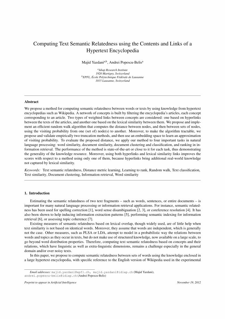
We propose an ad-hoc measure offering a better illustration of the network’s topology, aimed at finding out whetherthe graph is clustered or not – i.e., whether the communities of nodes based on neighborhoods have a preferred size,or are uniformly distributed. We consider a sample of 1000 nodes. For each node of the graph, the PersonalizedPageRank algorithm [32] is initialized from that node and run, thus resulting into a proximity coefficient for eachnode in the graph to the initial node. This is first done using hyperlinks, and then using the content links. The

2Therefore, the outdegree of all nodes is 10, but as the indegree may vary (the number of incoming links), the graph is not strictly speaking a10-regular graph.

3An example of neighborhood according to our relatedness measure is however shown in Section 6.3.4For the content links, the coefficient was computed regardless of their weights. A recent proposal for computing it for weighted graphs could

be applied too [66].5The observed values, together with the power law degree distribution, suggest that our graph is a scale-free network – characterized by the

presence of “hub” nodes – or a small-world network [65]. However, it is not clear what impact these properties defined mainly for social networkswould have here.

8

community size for the node is computed by sorting all nodes with respect to their proximity and counting how manynodes contribute to 99% of the mass.

0 200 400 600 800 1000 12000

1

2

3

4

5

6

7

8

Size of community

Num

ber

of N

odes

(a) Hyperlink graph

0 10 20 30 40 50 60 70 800

10

20

30

40

50

60

70

80

Size of community

Num

ber

of N

odes

(b) Content link graph

Figure 1: Distribution of community sizes for a sample of 1000 nodes (see text for the definition of a community). For each community size(x-axis) the graphs show the number of nodes (y-axis) having a community of that size, for each of the two graphs built from Wikipedia. Bothgraphs have a tendency towards clustering, i.e. a non-uniform distribution of links, with an average cluster size of 150–400 for hyperlinks and 7–14for content links.

The results shown in Figure 1 show that the distribution is neither flat nor uniformly decreasing, but has a peak,which provides an indication of the average size of clusters. This size is around 150–400 nodes for the hyperlinkgraph, without a sharp maximum, showing less clustering than for content links, for which this average is around7–14 nodes. The latter value is partly related to the 10-link limit set for content links, but is not entirely due to it, asthe limit concerns only outgoing links. The use of hyperlinks thus avoids local clusters and extends considerably theconnectivity of the network in comparison to content similarity ones.

5. Mapping Text Fragments to Concepts in the Network

In order to use the concept network for similarity judgments between two text fragments, two operations arenecessary, as explained at the end of Section 2.2. The first one, mapping each text fragment to a set of vertices of thenetwork, is explained in this section, while Sections 6 and 7 define the distance between two weighted sets of vertices.For mapping, two cases must be considered, according to whether the text matches exactly the title of a Wikipediapage or not. Exact matching is likely to occur with individual words or short phrases, but not with entire sentences orlonger texts.

If a text fragment consists of a single word or a phrase that matches exactly the title of a Wikipedia page, thenit is simply mapped to that concept. In the case of words or phrases that may refer to several concepts in Wikipe-dia, we simply assign to them the same page as the one assigned by the Wikipedia contributors as the most salientor preferred sense or denotation. For instance, ‘mouse’ directs to the page about the animal, which contains anindication that the ‘mouse (computing)’ page describes the pointing device, and that other senses are listed on the‘mouse (disambiguation)’ page. So, here, we simply map ‘mouse’ to the animal concept. However, for other words,no sense or denotation is preferred by the Wikipedia contributors, e.g. for the word ‘plate’. In such cases, a disam-biguation page is associated to that word or phrase. We chose not to include such pages in our network, as they do notcorrespond to individual concepts. So, in order to select the referent page for such words, we simply use the lexicalsimilarity approach described in the next paragraph.

When a fragment (a word, phrase, sentence, or text) does not match exactly the Wikipedia title of a vertex inour network, it is mapped to the network by computing its lexical similarity with the text content of the vertices inthe network, using cosine distance over stemmed words, stopwords being removed. Concept names (principal and

9

secondary ones) are given twice as much weight as the words found in the description of the concept. The textfragment is mapped to the k most similar articles according to this similarity score, resulting in a set of at most kweighted concepts. The weights are normalized, summing up to one, therefore the text representation in the networkis a probability distribution over at most k concepts. Finding the k closest articles according to lexical similarity canbe done efficiently using the Apache Lucene search engine (see note 1).

For example, consider the following text fragment to be mapped to our network: “Facebook: you have someserious privacy and security problems.” When this fragment is mapped to the k = 10 most similar Wikipedia ar-ticles, the resulting probability distribution is the following one: ‘Facebook’ (0.180), ‘Facebook Beacon’ (0.119),‘Facebook history’ (0.116), ‘Criticism of Facebook’ (0.116), ‘Facebook features’ (0.116), ‘Privacy’ (0.084), ‘PrivacyInternational’ (0.080), ‘Internet privacy’ (0.080), ‘Privacy policy’ (0.054), ‘Privacy Lost’ (0.054).

This mapping algorithm has an important role in the performance of the final system, in combination with thenetwork distance described hereafter. It must however be noted that the effects of wrong mappings at this stage arecountered later on. For instance, when large sets of concepts related to two text fragments are compared, a fewindividual mistakes are not likely to alter the overall relatedness scores. Alternatively, when comparing individualwords, wrong mappings are less likely to occur because the test sets for word similarity described in Section 10,page 17, also consider implicitly the most salient sense of each word, just as described above for Wikipedia.

6. Semantic Relatedness using Visiting Probability

In this section, we describe our framework for computing relatedness between two texts, represented as sets ofconcepts in a network. Although this is applied here to Wikipedia, the model is general enough to be applied toother networks too. The goal is to estimate a distance between two concepts or two sets of concepts that capturestheir relatedness by taking into account the global connectivity of the network, and without being biased by localproperties. Indeed, the use of individual links and paths, e.g. when estimating conceptual relatedness as the length ofshortest path, does not take into account their relative importance with respect to the overall properties of the network,such as the number and length of all possible paths between two nodes. Moreover, the length of the shortest pathis quite sensitive to spurious links, which are frequent in Wikipedia. Therefore, a number of aggregated proximitymeasures have been proposed, including PageRank and hitting time, as reviewed in Section 3 above.

Our proposal uses a random walk approach, and defines the relatedness of concept sets as the visiting probability,in the long run, of a random walker going from one set of nodes to the other one. The walker can use either type ofdirected links between concepts described in Section 4.2, i.e. hyperlinks or lexical similarity ones. This algorithm isindependent from the mapping algorithm introduced in the previous section.

6.1. Notations

Let S = {si|1 ≤ i ≤ n} be the set of n concepts or vertices in the network. Any two concepts si and s j can beconnected by one or more directed and weighted links, which can be of L different types (L = 2 in our case: hyperlinksand lexical similarity links). The structure of links of type l (1 ≤ l ≤ L) is fully described by the matrix Al of size n×n,where Al(i, j) is the weight of the link of type l between si and s j, with possible weights being 0 or 1 for the hyperlinkmatrix, and actual lexical similarity scores (or 0) for the content similarity matrix. The transition matrix Cl gives theprobability of a direct (one step) transition between concepts si and s j, using only links of type l. This matrix can bebuilt from the Al matrix as follows:

Cl(i, j) =Al(i, j)∑n

k=1 Al(i, k)

In the random walk process using all link types (1 ≤ l ≤ L), let the weight wl denote the importance of link typel. Then, the overall transition matrix C which gives the transition probability Ci, j between any concepts si and s j isC =∑L

l=1 wlCl.Finally, let ~r be the n-dimensional vector resulting from mapping a text fragment to the concepts of the network

(Section 5), which indicates the probabilities of concepts in the network given a text, or the relevance of concepts tothe text’s words. The sum of its elements is 1.

10

6.2. Definition of Visiting ProbabilityGiven a probability distribution ~r over concepts (i.e. a weighted set of concepts), and a concept s j in the network,

we first compute the probability of visiting s j for the first time when a random walker starts from ~r in the network,i.e. from any of the concepts in ~r that have a non-zero probability.6 To compute visiting probability, the followingprocedure provides a model of the state S t of the random walker, i.e. the concept in which the random walker ispositioned. Executing the procedure until termination gives the visiting probability VP.

Step 0: Choose the initial state of the walker with probability P(S 0 = si|~r) = ri. In other words, position the randomwalker on any of the concepts of ~r with the probability stated in ~r.

Step t: Assuming S t−1 is determined, if S t−1 = s j then return ‘success’ and finish the procedure. Otherwise, withprobability α, choose a value for the next concept S t according to the transition matrix C, and with probability1 − α, return ‘fail’. The possibility of ‘failing’, or absorption probability, introduces a penalty over long pathsthat makes them less probable.

We introduce C′ as being equal to the transition matrix C, except that in row j, C′( j, k) = 0 for all k. This indicatesthe fact that when the random walker visits s j for the first time, it can not exit from it and its probability mass drops tozero in the next step. This modified transition matrix was defined to account for the definition of visiting probabilityas the probability of first visit of s j (a similar idea has been proposed by Sarkar and Moore [62]).

To compute the probability of success in the above process, we introduce the probability of success at step t,pt(success), which is pt(success) = αt(~rC′t) j. In this formula, (~rC′t) j is the jth element of the vector ~rC′t, and C′t

is the power t of matrix C′. Then, the probability of success in the process, i.e. the probability of visiting s j startingfrom ~r, is the sum over all probabilities of success with different lengths:

p(success) =∞∑

t=0

pt(success) =∞∑

t=0

αt(~rC′t) j.

The visiting probability of s j starting from the distribution ~r, as computed above, is different from the probabilityassigned to s j after running Personalized PageRank (PPR) with a teleport vector equal to ~r. In the computation of VP,the loops starting from s j and ending to s j do not have any effect on the final score, unlike the computation of PPR,for which such loops boost the probability of s j. If some pages have this type of loops (typically “popular” pages),then after using PPR they will have high probability although they might not be very close to the teleport vector ~r.

The visiting probability of s j is also different from the hitting time to s j, defined as the average number of steps arandom walker would take to visit s j for the first time in the graph. If we use the same notations, the hitting time from~r to s j is H(~r, s j) =

∑∞t=0 t(~rC′t) j. Hitting time is more sensitive to long paths in comparison to VP (t in comparison

with αt in the formula), which might introduce more noise, while VP reduces the effect of long paths sooner in thewalk. We have compared the performance of these three algorithms in a previous paper [45] and concluded that VPoutperformed PPR and hitting time, which will not be used here.

6.3. Visiting Probability to Weighted Sets of Concepts and to TextsTo compute the VP from a weighted set of concepts to another set, i.e. from distribution ~r1 to distribution ~r2,

we construct a virtual node representing ~r2 in the network, noted sR(~r2). We then connect all concepts si to sR(~r2)according to the weights in ~r2. We now create the transition matrix C′ by adding a new row (numbered nR) to thetransition matrix C with all elements zero to indicate sR(~r2), then adding a new column with the weights in sR(~r2), andupdating all the other rows of C as follows (Ci j is an element of C):

C′i j = Ci j(1 − (~r2)i) for i, j , nR

C′inR= (~r2)i for all i

C′nR j = 0 for all j.

6A simpler derivation could first be given for the visiting probability to s j starting from another concept si, but to avoid duplication of equations,we provide directly the formula for a weighted set of concepts.

11

These modifications to the graph are local and can be done at run time, with the possibility to undo them for subsequenttext fragments to be compared.

To compute relatedness between two texts, we average between the visiting probability of ~r1 given ~r2 (notedVP(~r2,~r1)) and the visiting probability of ~r2 given ~r1 (noted VP(~r1,~r2)). A larger value of the measure indicates closerrelatedness. It is worth mentioning that (2− (VP(~r1,~r2)+VP(~r2,~r1)) is a metric distance, as it satisfies four properties:non-negativity, identity of indiscernible, symmetry, and triangle inequality, as it can be shown using the definition ofVP.

6.4. Illustration of Visiting Probability ‘to’ vs. ‘from’ a TextTo illustrate the difference between VP to and from a text fragment, we consider the following example. Though

any text fragment could be used, we took the definition of ‘jaguar’ (animal) from the corresponding Wikipedia article.Although the word ‘jaguar’ is polysemous, the topic of this particular text fragment is not ambiguous to a humanreader. The text was first mapped to Wikipedia as described above. Then, using VP with equal weights on hyperlinksand content links, the ten closest concepts (i.e. Wikipedia pages) in terms of VP from the text, and respectively to it,were found to be the following ones:

• Original text: “The jaguar is a big cat, a feline in the Panthera genus, and is the only Panthera species found inthe Americas. The jaguar is the third-largest feline after the tiger and the lion, and the largest in the WesternHemisphere.”

• Ten closest concepts according to their VP to the text: ‘John Varty’, ‘European Jaguar’, ‘Congolese SpottedLion’, ‘Lionhead rabbit’, ‘Panthera leo fossilis’, ‘Tigon’, ‘Panthera hybrid’, ‘Parc des Felins’, ‘Marozi’, ‘CraigBusch’.

• Ten closest concepts according to their VP from the text: ‘Felidae’, ‘Kodkod’, ‘North Africa’, ‘Jaguar’, ‘Pan-thera’, ‘Algeria’, ‘Tiger’, ‘Lion’, ‘Panthera hybrid’, ‘Djemila’.

The closest concepts according to VP from a text tend to be more general than closest concepts according to VPto the text. For instance, the second list above includes the genus and family of the jaguar species (Panthera andFelidae), while the first one includes six hybrid or extinct species related to the jaguar. Concepts close to a text thusbring detailed information related to the topics of the text, while concepts close from a text are more popular and moregeneral Wikipedia articles. Note also that none of the closest concepts above is related to the Jaguar car brand, asfound by examining each page, including the lesser-known ones (both persons cited are wildlife film makers and parkfounders). However, not all concepts are related in an obvious way (e.g. ‘Algeria’ is likely retrieved through ‘WesternHemisphere’).

The behavior illustrated on this example is expected given the definition of VP. A concept that is close to a text hasmore paths in the network towards the text with respect to other concepts in the network, which means that the conceptis quite specific in relation to the topics in the text, as in the above example. Conversely, a concept that is close from atext (in terms of VP from a text) is typically related by many paths from the text to the concept, in comparison to otherconcepts. This generally means that it is likely that the article is a general and popular article around the topics of thetext. If we consider the hierarchy between concepts from more general to more specific ones, then concepts close toa text are generally lower in the hierarchy with respect to the text, and concepts close from a text are generally higher.

7. Approximations: T-Truncated and ε-Truncated Visiting Probability

The above definition of the random walk procedure has one direct consequence: computation can be done iter-atively and can be truncated after T steps when needed, especially to maintain computation time within acceptablelimits. Truncation makes sense as higher order terms (for longer paths) get smaller with larger values of t becauseof the αt factor. Moreover, besides making computation tractable, truncation reduces the effect of longer (hence lessreliable) paths on the computed value of p(success). Indeed, VP to popular vertices (i.e. to which many links point)might be quite high even when they are not really close to the starting distribution ~r, due to the high number of longpaths toward them, and truncation conveniently reduces the importance of such vertices. We propose in this sectiontwo methods for truncating VP, and justify empirically the level of approximation chosen for our tasks.

12

T-truncated Visiting Probability. The simplest method, called T -truncated VP, truncates the computation for all thepaths longer than T . To compute an upper bound on the error of this truncation, we start by considering the possiblestate of the random walk at time T : either a success, or a failure, or a particular node. The sum of the probabilitiesof these three states equals 1, while the third value, i.e. the probability of returning neither success nor failure in thefirst t steps, can be computed as

∑ni, j α

t(~rC′t)i – this is in fact the probability mass at time t at all nodes except s j,the targeted node. If pT (success) denotes the probability of success considering paths of length at most T , and εT theerror made by truncating after step T , then by replacing pT (success) with the value we just computed, and noting thatp(success) + pT ( f ailure) ≤ 1, we obtain the following upper bound for εT :

εT = p(success) − pT (success) ≤n∑

i, j

αT (~rC′T )i.

So, if pT (success) is used as an approximation for p(success) then an upper bound for this approximation error εT isthe right term of the above inequality. This term decreases over time because αT and

∑ni, j(rC′T )i are both decreasing

over time, therefore εT decreases when T increases.

ε-truncated Visiting Probability. A second approach, referred to as ε-truncated VP, truncates paths with lower prob-abilities in earlier steps and lets paths with higher probabilities continue more steps. Given that the probability ofbeing at si at time step t is αt(rC′t)i, if this is neglected and set to zero, then the error caused by this approximationis αt(rC′t)i. Setting this term to zero means exactly that paths that are at si at time step t are no longer followedafterwards. So, in ε-truncation, paths with a probability less than ε are not followed, i.e. when αt(rC′t)i ≤ ε. Thisapproach is faster to compute than the previous one, but no upper bound of the error could be established. We use theε-truncated VP in some of our experiments below, leading to competitive results in an acceptable computation time.

T-Truncated Visiting Probability from all Vertices to a Vertex. Given a dataset of N documents, some tasks suchas document clustering (Section 12) require to compute the average VP between all N documents. Similarly, forinformation retrieval (Section 14), it is necessary to sort all the documents in a repository according to their relatednessto a given query. It is not tractable to compute exact VP values for all concepts, but we provide here a way to computeT -truncated VP from/to a distribution ~r for all concepts in the network, which is faster than repeating the computationfor each concept in part.

As in Section 6.3 above, we consider the virtual concept sR(~r) representing ~r in the network (noted simply sR). Itis then possible to compute VP from all concepts towards sR at the same time, using the following recursive procedureto compute the T -truncated visiting probability VPT . This procedure follows from the recursive definition of VP givenin Section 6.2, which states that VP(si, sR) = α

∑k C′(si, sk)VP(sk, sR). Therefore,

VPT (si, sR) = α∑

k C′(si, sk)VPT−1(sk, sR) for i , nR

VPT (si, sR) = 1 for i = nR

VP0(si, sR) = 0.

Using dynamic programming, it is possible to compute T -truncated VP from all concepts to sR in O(ET ) steps, whereE is the number of edges of the network.

T-Truncated Visiting Probability from a Vertex to all Vertices. Conversely, to compute VPT from ~r to all conceptsin the network, the total computation time is O(NET), where N is the number of concepts and E the number ofedges, because VPT must be computed for each concept. With our current network, this is very time consuming:therefore, we propose the following sampling method to approximate T -truncated VP. The sampling involves runningM independent T -length random walks from ~r. To approximate VPT to concept s j from ~r, if s j has been visited forthe first time at {tk1 , · · · , tkm } time steps in the M samples, then the T -truncated VP to s j can be approximated by thefollowing average: ˆVPT (~r, s j) = (

∑l α

tkl )/M.According to the proposed method, it is possible to approximate truncated VP from~r to all concepts in the network

in O(MT) time, where M is number of samples. It remains to find out how many samples should be used to obtainthe desired approximation level, a question that is answered by the following theorem. For any vertex, the estimatedtruncated VP approximates the exact truncated VPT to that vertex within ε with a probability larger than 1 − δ if thenumber of samples M is larger than α

2 ln(2n/δ)2ε2 . The proof of this result is given in Appendix A.

13

8. Empirical Analyses of VP and Approximations

We now analyze the convergence of the two approximation methods proposed above, i.e. the variation of themargin of error with T or ε. In the case of T -truncated approximation, when T increases to infinity, the T -truncatedapproximated VP converges towards the exact value, but computation time increases linearly with T . In the case ofε-truncation, when ε tends to zero the approximated value converges towards the real one, but again computation timeincreases. Therefore, we need to find the proper values for T and ε as a compromise between the estimated error andthe computing time.

8.1. Convergence of the T-Truncated VP over WikipediaThe value of T required for a certain level of convergence (upper bound on the approximation error) depends on

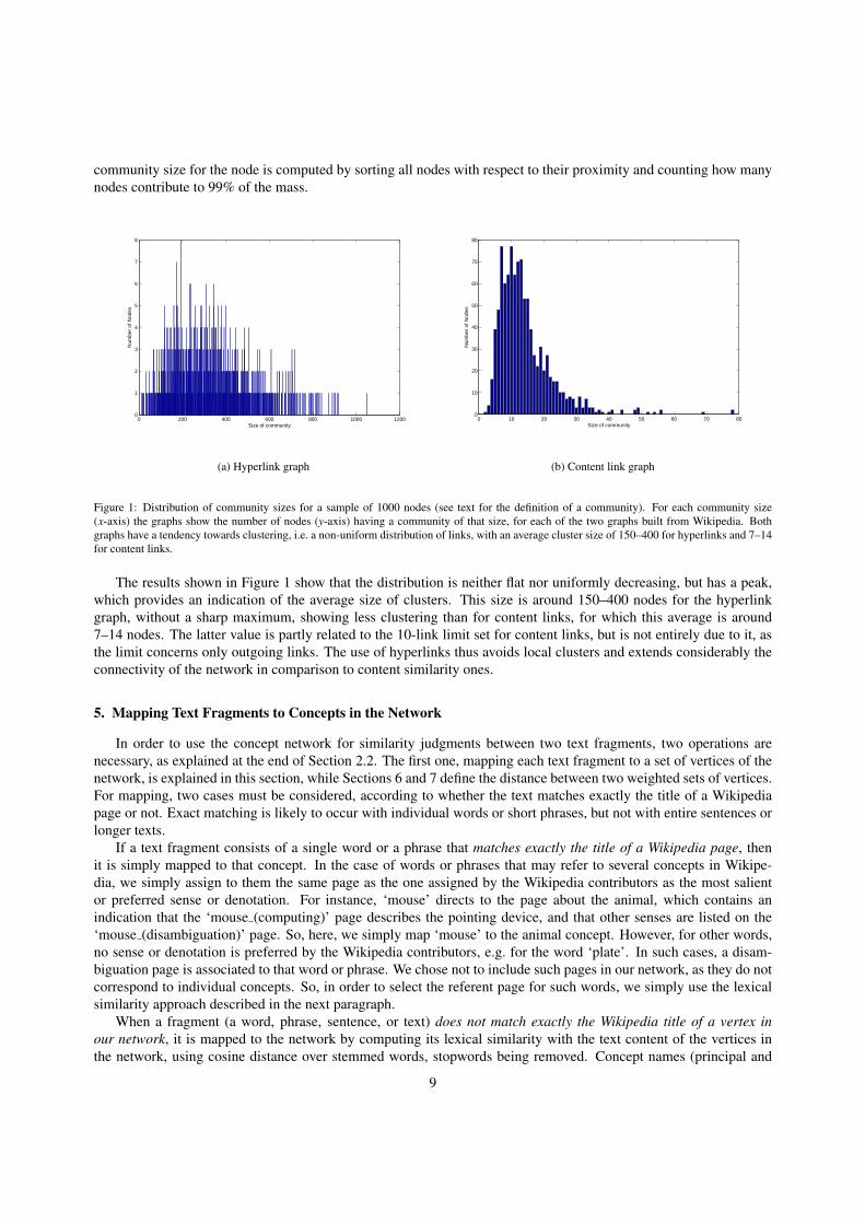
the transition matrix of the graph. It was not possible to find a convenient theoretical upper bound, so we analyzedthe relation between T and the approximation error empirically, by a sampling method. We chose randomly a set Sof 1000 nodes in the graph, and computed the T -truncated VP from all nodes in the graph to each of the nodes inS . Then we computed the average of the values of T -truncated VP from all nodes to the nodes in S : VPsum(T ) =∑

j∈S∑

i, j VPT (i, j)/|S |.Given that S is a large random sample, we consider that the evolution of VPsum(T ) with T is representative of the

evolution of an “average” VPT with T . Figure 2(a) shows the values of VPsum(T ) depending on T for the Wikipediagraph with the lexical similarity (content) links, for various values of α. Figure 2(b) shows the same curves for theWikipedia graph with hyperlinks. Both analyses show, as expected, that larger values of α correspond to a slowerconvergence in terms of T , because a larger α requires the random walker to explore longer paths for the same levelof approximation. (The exact value toward which VPsum(T ) converges is not important here.) The figures give someindication, for each given α, of the extent to which the paths should be explored for an acceptable approximation ofthe non-truncated VP value. In our experiments, we chose α = 0.8 and T = 10 as a compromise between computationtime and accuracy – the approximation error is less than 10% in Figures 2(a) and 2(b).

0 2 4 6 8 10 12 14 16 18 201

1.5

2

2.5

3

3.5

4

4.5

T

Sum

of V

P

alpha = 0.4

alpha = 0.5

alpha = 0.6

alpha = 0.7

alpha = 0.8

alpha = 0.9

(a) Content link graph

0 2 4 6 8 10 12 14 16 18 201

2

3

4

5

6

7

T

sum

of V

P

alpha = 0.4

alpha = 0.5

alpha = 0.6

alpha = 0.7

alpha = 0.8

alpha = 0.9

(b) Hyperlink graph

Figure 2: VPsum(T ) as an “average VP” for content links (a) and hyperlinks (b) over the Wikipedia graph, depending on T , for α varying from 0.4to 0.9 (by 0.1, bottom to top). The shape of the curves indicates the values of T leading to an acceptable approximation of the exact, non-truncatedvalue: α = 0.8 and T = 10 were chosen in the subsequent experiments.

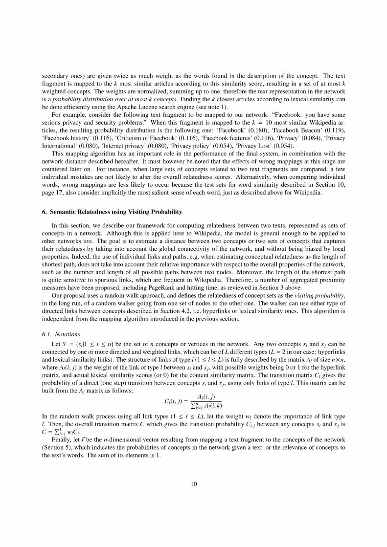
8.2. Convergence of ε-Truncated VP over WikipediaTo analyze the error induced by ε-truncation when computing VP over the Wikipedia graph, we proceeded in a

similar way. We chose 5000 random pairs of nodes and computed the sum of ε-truncated VP between each pair.Figure 3(a) shows the values of the sum depending on 1/ε for the Wikipedia graph with content links, and Figure 3(b)for the Wikipedia graph with the hyperlinks. Again, it appears from the curves that for a larger α, smaller values ofε are needed to reach the same level of approximation error, because for a larger α longer paths must be explored toreach the same approximation level. The ε-truncation is used for word similarity and document similarity below, witha value of ε = 10−5, and a value of α = 0.8 as above.

14

0 1 2 3 4 5 6 7 8 9 10

x 105

0

0.002

0.004

0.006

0.008

0.01

0.012

0.014

0.016

1/epsilon

alpha = 0.6alpha = 0.7alpha = 0.8alpha = 0.9

(a) Content link graph

0 1 2 3 4 5 6 7 8 9 10

x 105

0.025

0.03

0.035

0.04

0.045

0.05

0.055

0.06

1/epsilon

alpha = 0.6alpha = 0.7alpha = 0.8alpha = 0.9

(b) Hyperlink graph

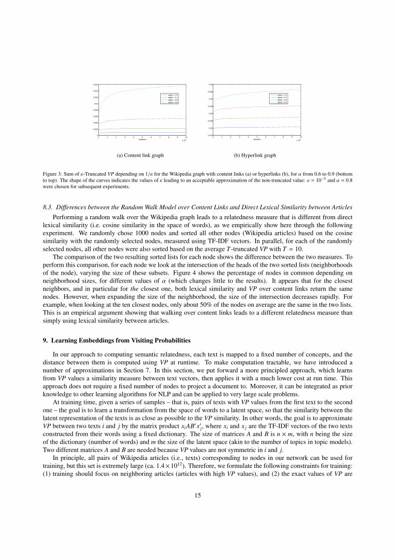
Figure 3: Sum of ε-Truncated VP depending on 1/ε for the Wikipedia graph with content links (a) or hyperlinks (b), for α from 0.6 to 0.9 (bottomto top). The shape of the curves indicates the values of ε leading to an acceptable approximation of the non-truncated value: ε = 10−5 and α = 0.8were chosen for subsequent experiments.

8.3. Differences between the Random Walk Model over Content Links and Direct Lexical Similarity between Articles

Performing a random walk over the Wikipedia graph leads to a relatedness measure that is different from directlexical similarity (i.e. cosine similarity in the space of words), as we empirically show here through the followingexperiment. We randomly chose 1000 nodes and sorted all other nodes (Wikipedia articles) based on the cosinesimilarity with the randomly selected nodes, measured using TF-IDF vectors. In parallel, for each of the randomlyselected nodes, all other nodes were also sorted based on the average T -truncated VP with T = 10.

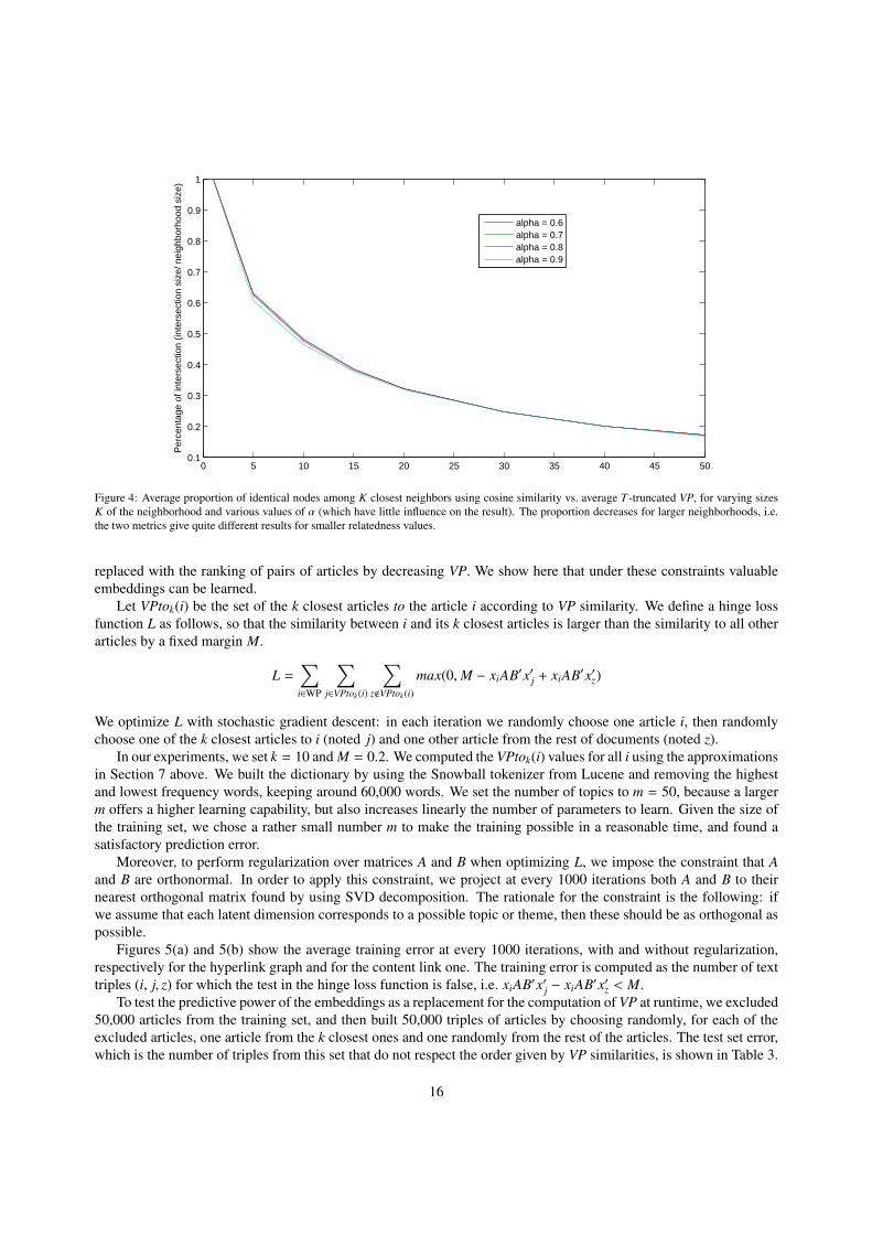
The comparison of the two resulting sorted lists for each node shows the difference between the two measures. Toperform this comparison, for each node we look at the intersection of the heads of the two sorted lists (neighborhoodsof the node), varying the size of these subsets. Figure 4 shows the percentage of nodes in common depending onneighborhood sizes, for different values of α (which changes little to the results). It appears that for the closestneighbors, and in particular for the closest one, both lexical similarity and VP over content links return the samenodes. However, when expanding the size of the neighborhood, the size of the intersection decreases rapidly. Forexample, when looking at the ten closest nodes, only about 50% of the nodes on average are the same in the two lists.This is an empirical argument showing that walking over content links leads to a different relatedness measure thansimply using lexical similarity between articles.

9. Learning Embeddings from Visiting Probabilities

In our approach to computing semantic relatedness, each text is mapped to a fixed number of concepts, and thedistance between them is computed using VP at runtime. To make computation tractable, we have introduced anumber of approximations in Section 7. In this section, we put forward a more principled approach, which learnsfrom VP values a similarity measure between text vectors, then applies it with a much lower cost at run time. Thisapproach does not require a fixed number of nodes to project a document to. Moreover, it can be integrated as priorknowledge to other learning algorithms for NLP and can be applied to very large scale problems.

At training time, given a series of samples – that is, pairs of texts with VP values from the first text to the secondone – the goal is to learn a transformation from the space of words to a latent space, so that the similarity between thelatent representation of the texts is as close as possible to the VP similarity. In other words, the goal is to approximateVP between two texts i and j by the matrix product xiAB′x′j, where xi and x j are the TF-IDF vectors of the two textsconstructed from their words using a fixed dictionary. The size of matrices A and B is n × m, with n being the sizeof the dictionary (number of words) and m the size of the latent space (akin to the number of topics in topic models).Two different matrices A and B are needed because VP values are not symmetric in i and j.

In principle, all pairs of Wikipedia articles (i.e., texts) corresponding to nodes in our network can be used fortraining, but this set is extremely large (ca. 1.4× 1012). Therefore, we formulate the following constraints for training:(1) training should focus on neighboring articles (articles with high VP values), and (2) the exact values of VP are

15

0 5 10 15 20 25 30 35 40 45 500.1

0.2

0.3

0.4

0.5

0.6

0.7

0.8

0.9

1

K closest

Per

cent

age

of in

ters

ectio

n (in

ters

ectio

n si

ze/ n

eigh

borh

ood

size

)

alpha = 0.6alpha = 0.7alpha = 0.8alpha = 0.9

Figure 4: Average proportion of identical nodes among K closest neighbors using cosine similarity vs. average T -truncated VP, for varying sizesK of the neighborhood and various values of α (which have little influence on the result). The proportion decreases for larger neighborhoods, i.e.the two metrics give quite different results for smaller relatedness values.

replaced with the ranking of pairs of articles by decreasing VP. We show here that under these constraints valuableembeddings can be learned.

Let VPtok(i) be the set of the k closest articles to the article i according to VP similarity. We define a hinge lossfunction L as follows, so that the similarity between i and its k closest articles is larger than the similarity to all otherarticles by a fixed margin M.

L =∑i∈WP

∑j∈VPtok(i)

∑z<VPtok(i)

max(0,M − xiAB′x′j + xiAB′x′z)

We optimize L with stochastic gradient descent: in each iteration we randomly choose one article i, then randomlychoose one of the k closest articles to i (noted j) and one other article from the rest of documents (noted z).

In our experiments, we set k = 10 and M = 0.2. We computed the VPtok(i) values for all i using the approximationsin Section 7 above. We built the dictionary by using the Snowball tokenizer from Lucene and removing the highestand lowest frequency words, keeping around 60,000 words. We set the number of topics to m = 50, because a largerm offers a higher learning capability, but also increases linearly the number of parameters to learn. Given the size ofthe training set, we chose a rather small number m to make the training possible in a reasonable time, and found asatisfactory prediction error.

Moreover, to perform regularization over matrices A and B when optimizing L, we impose the constraint that Aand B are orthonormal. In order to apply this constraint, we project at every 1000 iterations both A and B to theirnearest orthogonal matrix found by using SVD decomposition. The rationale for the constraint is the following: ifwe assume that each latent dimension corresponds to a possible topic or theme, then these should be as orthogonal aspossible.

Figures 5(a) and 5(b) show the average training error at every 1000 iterations, with and without regularization,respectively for the hyperlink graph and for the content link one. The training error is computed as the number of texttriples (i, j, z) for which the test in the hinge loss function is false, i.e. xiAB′x′j − xiAB′x′z < M.

To test the predictive power of the embeddings as a replacement for the computation of VP at runtime, we excluded50,000 articles from the training set, and then built 50,000 triples of articles by choosing randomly, for each of theexcluded articles, one article from the k closest ones and one randomly from the rest of the articles. The test set error,which is the number of triples from this set that do not respect the order given by VP similarities, is shown in Table 3.

16

0 500 1000 1500 2000 25000.1

0.2

0.3

0.4

0.5

0.6

0.7

0.8

0.9

1

HyperErrorHyperErrorReg

(a) Hyperlink graph

0 500 1000 1500 2000 25000.1

0.2

0.3

0.4

0.5

0.6

0.7

0.8

0.9

1

LexErrorLexErrorReg

(b) Content link graph

Figure 5: Average training error for learning embeddings, measured every 1000 iterations, with and without using regularization.

Training set for embedding Error (%)Hyperlinks 9.8Hyperlinks with Regularization 13.5Content Links 5.4Content Links with Regularization 5.9

Table 3: Accuracy of embeddings learned over four different training sets. The error (percentage) is computed for 50,000 triples of articles from aseparate test set, as the number of triples that do not respect the ordering of VP similarities.

The two main findings are the following. First, VP over the hyperlinks graph is harder to learn, which may bedue to the fact that hyperlinks are defined by users in a manner that is not totally predictable. Second, regularizationdecreases the prediction ability. However, if regularization traded prediction power for more generality, in otherwords if it reduced overfitting to this problem and made the distance more general, then it would still constitute auseful operation. This will be checked in the experiments in Sections 12, 13 and 15. Moreover, these experimentswill show that the embeddings can be plugged into state-of-the-art learning algorithms as prior knowledge, improvingtheir performance.

10. Word Similarity

In the following sections, we assess the effectiveness of visiting probability by applying it to four language pro-cessing tasks. In particular, for each task, we examine each type of link separately and then compare the results withthose obtained for combinations of links, in the attempt to single out the optimal combinations.

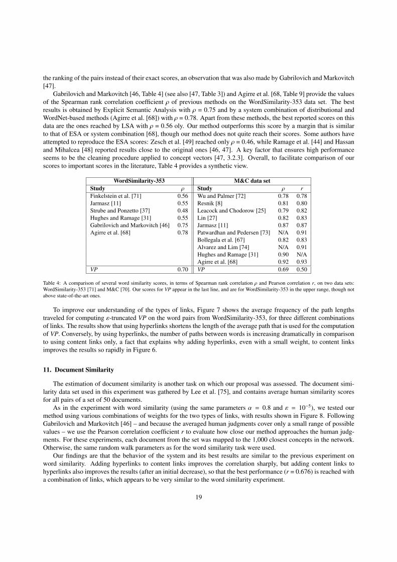
The word similarity task has been heavily researched using a variety of methods and resources – such as WordNet,Roget’s Thesaurus, the English Wikipedia or Wiktionary – starting for instance with Resnik’s seminal paper [8] andeven earlier. We have reviewed in Section 3 some of the recent work on word similarity, focusing mainly on graph-based methods over Wikipedia but also WordNet. Recent studies, including also references to previous scores andseveral baselines, have been made by Bollegala et al. [67], Gabrilovich and Markovitch [46] (see also [47, Tables 2and 3]), Zesch et al. [49], Agirre et al. [68], and Ramage et al. [44], among others.

Three test sets for the English word similarity task have been extensively used in the past. They consist ofpairs of words accompanied by average similarity scores assigned by human subjects to each pair. Depending onthe instructions given to the subjects, the notion of ‘similarity’ was sometimes rather interpreted as ‘relatedness’, asdiscussed for instance by Hughes and Ramage [31, Section 5]. The three sets, all of them reproduced in Jarmasz’sthesis [11] for instance, were designed respectively by Rubenstein and Goodenough [69] (henceforth, R&G, 65 pairs,

17

51 judges), by Miller and Charles [70] (M&C, 30 pairs), and by Finkelstein et al. [71] (WordSimilarity-353, with 353pairs).

We estimate the relatedness between words by mapping them to concepts and computing the ε-truncated VPdistance between them with ε = 10−5. We set the value of α = 0.8 as explained in Section 8.2 above. The correlationwith human judgments of relatedness is measured using the Spearman rank correlation coefficient ρ as well as thePearson correlation coefficient r between the VP values for each pair and the human judgments.

Figure 6: Spearman rank correlation ρ between automatic and human judgments of word similarity on the WordSimilarity-353 data set, dependingon the weight of content links in the random walk (the weight of hyperlinks is the complement to 1). The best scores, ρ = 0.70, are reached whencontent links have more weight than hyperlinks (0.7–0.8 vs. 0.3–0.2). The result of LSA, ρ = 0.56, is quoted from [46], and is outperformed byother scores in the literature.

The values of the Spearman rank correlation coefficient ρ on the WordSimilarity-353 data set, for varying relativeweights of content links vs. hyperlinks in the random walk, are shown in Figure 6. The best scores reach ρ = 0.70 for acombination of hyperlinks and content links, weighted between 0.3/0.7 and 0.2/0.8. As shown in the figure, results im-prove by combining links in comparison with using a single type. Results improve rapidly when hyperlinks are addedto content ones (right end of the curve), even with a small weight, which shows that adding encyclopedic knowledgerepresented by hyperlinks to word co-occurrence information can improve significantly the performance. Conversely,adding content links to hyperlinks also improves the results, likely because the effect of spurious hyperlinks is reducedafter adding content links.

To find out whether the two types of links encode similar relations or not, we examined to what extent resultsusing VP with hyperlinks only are correlated with results using content links only. The Spearman rank correlationcoefficient between these scores is ρ = 0.71, which shows that there is some independence between scores.

We also tested our method on the R&G and M&C data sets. The values of the Pearson correlation coefficient r forprevious algorithms using lexical resources are given by Jarmasz [11, Section 4.3.2], by Gabrilovich and Markovitch[47, Table 3] and by Agirre et al. [68, Table 7], showing again that for word similarity, using lexical resources is verysuccessful, reaching a correlation of 0.70–0.85 with human judgments. For our own algorithm, correlation r withhuman judgments on R&G and M&C is, respectively, 0.38–0.42 and 0.46–0.50, depending on the combination oflinks that is used. Lexically-based techniques are thus more successful on these data sets, for which only the lexicalsimilarity relation is important, while our method, which considers linguistic as well as extra-linguistic relations, isless efficient.

However, if we examine the Spearman rank correlation ρ on the R&G and M&C data sets, considering thereforeonly the ranking between pairs of words and not the exact values of the relatedness scores, then our method reaches0.67–0.69. Our scores are thus still lower than the best lexically-based techniques, which have a ρ between 0.74–0.81and 0.69–0.86 on R&G and M&C, but the difference is now smaller. Our method is thus more suitable for capturing

18

the ranking of the pairs instead of their exact scores, an observation that was also made by Gabrilovich and Markovitch[47].

Gabrilovich and Markovitch [46, Table 4] (see also [47, Table 3]) and Agirre et al. [68, Table 9] provide the valuesof the Spearman rank correlation coefficient ρ of previous methods on the WordSimilarity-353 data set. The bestresults is obtained by Explicit Semantic Analysis with ρ = 0.75 and by a system combination of distributional andWordNet-based methods (Agirre et al. [68]) with ρ = 0.78. Apart from these methods, the best reported scores on thisdata are the ones reached by LSA with ρ = 0.56 oly. Our method outperforms this score by a margin that is similarto that of ESA or system combination [68], though our method does not quite reach their scores. Some authors haveattempted to reproduce the ESA scores: Zesch et al. [49] reached only ρ = 0.46, while Ramage et al. [44] and Hassanand Mihalcea [48] reported results close to the original ones [46, 47]. A key factor that ensures high performanceseems to be the cleaning procedure applied to concept vectors [47, 3.2.3]. Overall, to facilitate comparison of ourscores to important scores in the literature, Table 4 provides a synthetic view.

WordSimilarity-353 M&C data setStudy ρ Study ρ rFinkelstein et al. [71] 0.56 Wu and Palmer [72] 0.78 0.78Jarmasz [11] 0.55 Resnik [8] 0.81 0.80Strube and Ponzetto [37] 0.48 Leacock and Chodorow [25] 0.79 0.82Hughes and Ramage [31] 0.55 Lin [27] 0.82 0.83Gabrilovich and Markovitch [46] 0.75 Jarmasz [11] 0.87 0.87Agirre et al. [68] 0.78 Patwardhan and Pedersen [73] N/A 0.91

Bollegala et al. [67] 0.82 0.83Alvarez and Lim [74] N/A 0.91Hughes and Ramage [31] 0.90 N/AAgirre et al. [68] 0.92 0.93

VP 0.70 VP 0.69 0.50

Table 4: A comparison of several word similarity scores, in terms of Spearman rank correlation ρ and Pearson correlation r, on two data sets:WordSimilarity-353 [71] and M&C [70]. Our scores for VP appear in the last line, and are for WordSimilarity-353 in the upper range, though notabove state-of-the-art ones.

To improve our understanding of the types of links, Figure 7 shows the average frequency of the path lengthstraveled for computing ε-truncated VP on the word pairs from WordSimilarity-353, for three different combinationsof links. The results show that using hyperlinks shortens the length of the average path that is used for the computationof VP. Conversely, by using hyperlinks, the number of paths between words is increasing dramatically in comparisonto using content links only, a fact that explains why adding hyperlinks, even with a small weight, to content linksimproves the results so rapidly in Figure 6.

11. Document Similarity

The estimation of document similarity is another task on which our proposal was assessed. The document simi-larity data set used in this experiment was gathered by Lee et al. [75], and contains average human similarity scoresfor all pairs of a set of 50 documents.

As in the experiment with word similarity (using the same parameters α = 0.8 and ε = 10−5), we tested ourmethod using various combinations of weights for the two types of links, with results shown in Figure 8. FollowingGabrilovich and Markovitch [46] – and because the averaged human judgments cover only a small range of possiblevalues – we use the Pearson correlation coefficient r to evaluate how close our method approaches the human judg-ments. For these experiments, each document from the set was mapped to the 1,000 closest concepts in the network.Otherwise, the same random walk parameters as for the word similarity task were used.

Our findings are that the behavior of the system and its best results are similar to the previous experiment onword similarity. Adding hyperlinks to content links improves the correlation sharply, but adding content links tohyperlinks also improves the results (after an initial decrease), so that the best performance (r = 0.676) is reached witha combination of links, which appears to be very similar to the word similarity experiment.

19

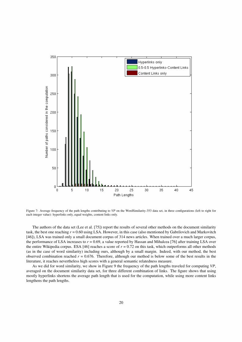
Figure 7: Average frequency of the path lengths contributing to VP on the WordSimilarity-353 data set, in three configurations (left to right foreach integer value): hyperlinks only, equal weights, content links only.

The authors of the data set (Lee et al. [75]) report the results of several other methods on the document similaritytask, the best one reaching r = 0.60 using LSA. However, in this case (also mentioned by Gabrilovich and Markovitch[46]), LSA was trained only a small document corpus of 314 news articles. When trained over a much larger corpus,the performance of LSA increases to r = 0.69, a value reported by Hassan and Mihalcea [76] after training LSA overthe entire Wikipedia corpus. ESA [46] reaches a score of r = 0.72 on this task, which outperforms all other methods(as in the case of word similarity) including ours, although by a small margin. Indeed, with our method, the bestobserved combination reached r = 0.676. Therefore, although our method is below some of the best results in theliterature, it reaches nevertheless high scores with a general semantic relatedness measure.

As we did for word similarity, we show in Figure 9 the frequency of the path lengths traveled for computing VP,averaged on the document similarity data set, for three different combination of links. The figure shows that usingmostly hyperlinks shortens the average path length that is used for the computation, while using more content linkslengthens the path lengths.

20

Figure 8: Pearson correlation coefficient r between VP results and human judgments on document similarity, depending on the weight of thehyperlinks in the combination (the weight of the content links is the complement to 1). The best score of r = 0.676 is reached when hyperlinks haveless weight than content links, but are still used. The result of LSA, r = 0.60, is quoted from Lee et al. [75].

12. Document Clustering

This section describes the experimental setting and the results of applying the text relatedness measure definedabove to the problem of document clustering over the 20 Newsgroups dataset.7 The dataset contains about 20,000postings to 20 news groups, hence 20 document classes with about 1,000 documents per class. We aim here at findingthese classes automatically, using for testing the entire data set without using any part of it as a training set. Theknowledge of our system comes entirely from the Wikipedia network and the techniques described in Sections 6–7for computing distances between two texts projected onto the network. We also experimented with the embeddingstrained over VP similarities described in Section 9.

12.1. Setup of Experiment on 20 NewsgroupsWe first compute a similarity matrix for the entire 20 Newsgroups data set, with the relatedness score between

any two documents being VPT . For tractability, we fixed T = 10, a value that gives sufficient precision, as studiedempirically in Section 8 above. Similarly, we empirically set the absorption probability of the random walk at 1−α =0.2. Based on α and T , the results in Section 7 allowed us to compute the error bound of the truncation. So, thechoice of α and T was also guided by the fact that for a smaller α, fewer steps (T ) are needed to achieve the sameapproximation precision because of the penalty set to longer paths. In this application, instead of computing VPT

between all possible pairs separately, we filled one row of the matrix at a time using the approximations we proposed.To use the embeddings we simply transform all the documents by the embeddings matrices and then run the clusteringalgorithm over the transformed documents in the projection space. We trained two matrices, A and B, for eachWikipedia graph. The qualitative behavior of the results by using A and B is very similar. Here we report only theresults of the transformation by A to help readability of the results.

Clustering is performed using a k-means algorithm over each of the similarity matrices and feature representations.The similarity metric between two representation vectors is cosine similarity. Given the randomized initialization ofthe algorithm, the final clusterings are different in each run of the algorithm.

The quality of the clustering is measured using the Rand Index (RI), which counts the proportion of pairs ofdocuments that are similarly grouped, i.e. either in the same, or in different clusters, in the reference vs. candidateclusterings. RI tends to penalize the smaller clusters, for example if the algorithm clusters together two classes and

7The dataset is distributed at http://www.cs.cmu.edu/afs/cs.cmu.edu/project/theo-20/www/data/news20.html, see also [77, Chapter 6].

21

Figure 9: Frequencies of the path lengths contributing to VP, averaged over the document similarity data set, in three configurations of the system(left to right for each integer value): hyperlinks only, content links only, and equal weights for both types.

splits another class, it will receive a high penalty from RI. This happens often in 20 Newsgroups data set, given thatsome classes are very similar and some other classes are more general and potentially suitable for splitting. As aconsequence, the RI values vary largely from one run to another run, making significance testing quite difficult. Togain more information about the quality of the clustering, we consider precision, recall and F-score.

Table 5 shows average results (over ten runs) of the clustering algorithm using various relatedness measures. Therandom walk model significantly outperforms the baseline cosine similarity between TF-IDF vectors for documentclustering, and it also outperforms LSA in terms of F-score, with most of the relatedness measures. The RI scores donot allow conclusions as their variation does not allow significance judgments. The comparison with previous workis uneasy, as no systematic comparison of clustering methods on the 20 Newsgroups datasets was known to us. Ina recent paper, Hu et al. [78] found an F-score of 14.8% for a baseline word vector method, improved to 19.6% bytheir use of Wikipedia, for agglomerative clustering. However, for partitional clustering with K-means, both scoresincreased more than twice (to 38.2% for the baseline and 41.8% for their best method), a result that could not beconfirmed independently.

For our approach, the combination of hyperlinks and content links improves the results over using either of themalone. Using the embeddings of the content links reduces the performance in comparison to the computation of the

22

Distance Metric Precision Recall F-score RICosine similarity of TF-IDF vectors 9.29 19.04 12.49 86.67LSA 19.10 20.64 19.84 91.67VP on content links 24.13 37.15 29.13 90.94VP on hyperlinks 18.36 39.22 24.72 87.78VPComb (0.6 content links) 24.26 36.91 29.23 91.03Embedding from content links (ECL) 21.30 26.13 23.47 91.48Embedding from hyperlinks (EHL) 22.63 28.40 25.17 91.56ECL with regularization 22.74 27.67 24.95 91.68EHL with regularization 24.08 29.64 26.56 91.80

Table 5: Rand Index (RI), precision, recall and F-score of different clustering methods. VPComb stands for VP over a combination of content links(weighted 0.6) and hyperlinks (0.4). Scores in bold are significantly higher than LSA, the one in italics significantly lower (t-test, p < 0.001).

VP values over the graph. On the contrary, using embeddings of the hyperlinks improves the results in comparison tousing the VP values over the hyperlinks graph.

The embedding learned on VP similarities over the hyperlinks appears to provide a more general similarity mea-sure, with does not overfit to the Hyperlinks graph of Wikipedia. The high recall it obtains is related to the largerextension of paths computed with hyperlinks, which can connect many documents together and attach them to thesame class, while the high precision obtained using content links is due to their tendency to cluster into smallerneighborhoods.

Although the regularization imposed on the embeddings reduced their predictive power for the VP similarities, butit improves the performance on this task.

Computation time using embeddings is (as expected) greatly reduced, as computations are performed in the low-dimensional latent space. Moreover, other unsupervised clustering algorithms can be applied to the documents trans-formed by the embeddings, e.g. the state-of-the-art clustering algorithm proposed by Bordogna and Pasi [79].

12.2. Comparison of VP and Cosine Similarity

To find out in which cases the proposed method improves over a simple cosine similarity measure, we considereda linear combination of the cosine similarity and VPComb (VP over content links weighed 0.6 and hyperlinks weighed0.4), namely w × VPComb + (1 − w) × LS, and varied the weight w from 0 to 1. Considering the k-nearest neighborsof every document according to this combined similarity, we define k-purity as the number of documents with thecorrect label over the total number of documents k in the computed neighborhood. The variation of k-purity with w,for several sample values of k, is shown in Figure 10.

The best purity appears to be obtained for a combination of the two methods, for all values of k that were tested.This shows that VPComb brings valuable additional information about document relatedness that cannot be found in LSonly. Furthermore, when the size of the examined neighborhood k increases (lower curves in Figure 10), the effect ofVPComb becomes more important, i.e. its weight in the optimal combination increases. For very small neighborhoods,LS is almost sufficient to ensure optimal purity, but for larger ones (k = 10 or 15), VPComb used alone (w = 1)outperforms LS used alone (w = 0). Their optimal combination leads to scores that are higher than those obtainedfor each of them used separately, and, as noted, the weight of VPComb in the optimal combination increases for largerneighborhoods.

These results can be explained as follows. For very small neighborhoods, the cosine lexical similarity score withthe nearest 1–5 documents is very high, as they have many words in common, so LS is a good measure of textrelatedness. However, when looking at larger neighborhoods, for which relatedness is less based on identical words,then VPComb becomes more effective, and LS performs poorly. Therefore, we can predict that VPComb will be mostrelevant when looking for larger neighborhoods, or in order to increase recall. VPComb should also be relevant whenthere is low diversity among document words, for instance when all documents are very short.

23

0 0.2 0.4 0.6 0.8 1 1.20

0.1

0.2

0.3

0.4

0.5

0.6

0.7

0.8

0.9

Weight of VP vs. Cosine Similarity

Ave

rage

pur

ity o

f nei

ghbo

rhoo

ds

1 nearest neighbor, max at w = 0.65 nearest neighbors, max at w = 0.710 nearest neighbors, max at w = 0.815 nearest neighbors, max at w=0.9

Figure 10: Values of k-purity (vertical axis) averaged over all documents, for neighborhoods of different sizes k. The horizontal axis indicates theweight w of visiting probability vs. cosine lexical similarity in the formula: w × VPComb + (1 − w) × LS.

13. Text Classification

We showed in the previous section that using the VP similarities over Wikipedia hyperlinks and content linksgraphs improved text clustering. Although text clustering is an important application, there have been more studies ontext classification, i.e. when labeled examples are available for learning. In this section, we investigate this problem byusing the embeddings that were learned over VP similarities in Section 9 above. Embeddings can easily be integratedwith any distance learning algorithm as prior knowledge or as an initial state. We thus designed a distance learningalgorithm for this purpose, which we compared (using various embeddings) to an SVM text classifier, outperformingits score when few training examples are available.

13.1. Distance Learning ClassifierWe built a distance learning classifier which learns, given a training set, a similarity measure so that for each

data point in the training set, its similarity to data points with the same label (or class) is higher than data pointswith different labels. This classifier is essentially very similar to a large margin nearest neighbor classifier [80], withsome changes that make it applicable to large scale text classification problems with a large number of features (here,words).

We define the similarity between two documents i and j represented by TF-IDF vectors xi and x j as xiAA′x′j ,where A is a matrix n × m, n being the size of the feature dictionary and m size of the latent space. If C(i) denotes theclass (label) of document i, then we define the following loss function L over the training set:

L =∑

i

∑C( j)=C(i)

∑C(z),C(i)

max(0,M − xiAA′x′j + xiAA′x′z)

M is a margin which is set to 0.2 in our experiments. We performed the optimization of L by stochastic gradient de-scent. At testing time, we proceeded similarly to the k-nearest neighbors algorithm: we chose the k closest documentsfrom the training set according to the learned distance and then returned the class (label) resulting from the majorityvote.

24

Our goal here is to show that starting from the prior knowledge obtained from VP similarities over Wikipediagraphs in the forms of the embeddings can improve the performance of the classification, especially when a smallnumber of training samples is available.

13.2. 20 Newsgroups Classification

We applied the above method to classify texts from the 20 Newsgroups data set. We compared the results ofthe distance learning algorithm, with various initial points, to a linear SVM method (LIBSVM implementation [81]),which is a state-of-the-art text classifier. The classification accuracy is given in Table 6 for various sizes of the trainingset. We have trained two matrices over VP similarities, A and B, because VP similarity is not symmetric. We haveexperimented with initialization by either A or B, which gives similar results, therefore we show only the results usingmatrix A. The distance learning classifier with random initialization of the parameters performed poorly, so it is notreported here.

Method Size of the training set40 100 200 500 800 1000 1500

DL + CL embedding 21.13 32.93 42.79 56.57 62.54 65.90 70.57DL + CL emb. + REG 22.54 34.14 44.32 57.12 63.82 66.43 71.10DL + HL embedding 21.40 34.31 44.09 57.18 63.09 66.31 70.65DL + HL emb. + REG 22.50 35.29 46.17 58.64 64.08 66.84 71.14SVM 7.90 15.93 28.48 52.40 61.76 65.67 70.83

Table 6: Classification accuracy for different sizes of the training set over the 20 Newsgroups data set. The accuracy is the average of 10 timesrun on a randomly divided data set. ‘DL’ is distance learning classifier, ‘CL’ is the embedding learned over the content links graph and ‘HL’ theembedding learned over hyperlinks, ‘REG’ stands for regularization of the matrix. The numbers in italics are significantly better than the accuracyof the SVM (t-test, p < 0.001)

.

The first important observation is that, when the training set is small, the distance learning classifier initialized withthe embeddings from VP similarities over Wikipedia graphs outperforms the baseline SVM classifier significantly. Byadding more and more labeled data, the importance of prior knowledge appears to decrease, presumably because thedistance learning algorithm can infer reliable decisions based only on the training data. A similar effect was shownfor a method based on deep learning by Ranzato and Szummer [82], with their method and a TF-IDF/SVM methodboth reaching 65% accuracy for more than 50 samples per class (corresponding to 1000 total samples) in the trainingdata.

The second observation is that the orthonormality regularization that we imposed on the embeddings again im-proved the performance. The generalization ability was improved at the price of decreasing slightly the precision inthe approximation of the VP values. A third observation is that the accuracy using hyperlinks was slightly higher thanusing content links.

14. Information Retrieval

In this section, we apply the proposed distance to information retrieval data from TREC-7 and TREC-8 [83]. Theapplication of our method to a large scale information retrieval task requires the computation of VP between a queryand the representation of all the documents in the repository. By using the approximations proposed in Section 7, wecan compute T -truncated VP between every query and documents in an acceptable amount of time. Firstly, we mapall documents in the data set to the Wikipedia graph; then, at query time, each query is mapped to the graph; finally,for each query, VPT is computed to and from all documents in the data set by using the proposed approximations.In this section, we use α = 0.8 , T = 10 and a combination of hyperlinks and content links in VP weighted 0.2/0.8,following observations from previous sections. The time-consuming operation is the first one – viz., mapping a largecollection of documents to the Wikipedia graph – but this is done only once, before query time.

25

We used the TREC-7 and TREC-8 Ad-hoc Test Collections.8 The data set includes a repository of 530,000 doc-uments and two sets of 50 queries. For each query, the data set also provides relevance judgments for a subset ofdocuments considered to be related to the query, as they were retrieved by a pool of search methods, a method thatis intended to maximize recall. To study the effect of VP in comparison to lexical similarity and TF-IDF scoring ina single retrieval operation, we compute for each document and query a linear combination of VPT with weight wand of lexical similarity with weight 1 − w. The weight w thus sets the relative importance of conceptual relatednessvs. lexical similarity, and will serve to illustrate their respective contributions. We will refer to this as the Combinedsimilarity. We measure the IR performance through the average precision of the first 10 returned documents (10 is thetypical size of the first result page of Web search engines).

We computed all the scores for w = 0 to w = 1 with increments of 0.1, and found out that the highest scorewas reached for w = 0.1 for the TREC-7 data set. This optimized value was then tested over the TREC-8 query set(50 topics), leading to an average precision for Combined of 0.515 , which improves (+15.4 %) over the precisionof lexical similarity alone (w = 0), which is 0.446. Egozi et al. [84] reported precision at 10 on TREC-8 data forvarious bag-of-words information retrieval systems (Xapian, Okapi, LM-KL-DIR) along with improved results (upto 14%) obtained by using a new retrieval algorithm, which integrates ESA [47] semantic similarity to the previoussystems.9 Here, we reported the mean average precision at 10, which is the lower bound of precision at 10, but ismore informative than it. Direct comparison between our scores and the scores reported in [84] is not possible, as theyused different base retrieval systems.

We also examined the precision score for every query separately. In particular, we counted the proportion ofqueries for which the Combined similarity returned more relevant documents than lexical similarity alone. Combinedsimilarity outperformed the lexical one on 14 queries, while the reverse was true for 5 queries only, and the scoreswere identical on the remaining 31 queries. The average score difference between Combined and lexical similarity is0.018 (maximum is 1). This value is not significantly above 0 at the usual levels (e.g. p < 0.01), but we found usinga normal distribution that the probability of the true difference being zero, given the observations, is only p = 0.11.While this does not ensure that the Combined similarity is “significantly” better than the lexical one, it still provideencouraging evidence for the utility of VP on the TREC-8 test set.

The precision scores of both methods vary considerably across queries. We therefore examined separately the“difficult” queries, defined here as the queries on which lexical similarity had a score of 0.3 or less (meaning itreturned between 0 and 3 relevant documents). There are 21 such queries out of 50 on the TREC-8 test set. Overthese queries, the Combined similarity outperforms the lexical one on 7, while the reverse is true for only one, and13 queries are a tie. Of course, it might seem unsurprising to see this difference as these queries are “difficult” forthe lexical similarity by definition. However, when examining the 20 queries that are “difficult” for the Combinedsimilarity, this measure still outperforms the lexical one on 5, while the reverse is true for only two, and 13 are a tie.These results show that VP provides complementary information that can improve the results of lexical similarity forIR, especially for queries on which lexical similarity performs less well.

15. Learning to Rank by Using VP Similarities

We have seen in the previous section that the linear combination of the VP and lexical similarities improved onlyslightly the retrieval results, although VP provides additional information. This motivated us to integrate the VPsimilarity to a learning to rank system [85], instead of a linear combination with lexical similarity. We have chosenan approach similar to the discriminative projection learning algorithm introduced by Yih et al. [86] which exhibitsgood performance. We have reimplemented the algorithm for the experiments in this section, and we first describe itbriefly, then discuss the results.

Assume that for a query q, a document dr is relevant and dnr is not relevant. The algorithm learns a projectionA from TF-IDF vectors of the articles to a latent space such that the similarity between the projections of q and dr

8These are available at http://trec.nist.gov, and we used more specifically the test queries (topics) numbers 351–400 and 401–450, with theassociated relevance judgments. The documents are available from the Linguistic Data Consortium.

9Precision at 10 was improved as follows: for Xapian from 0.472 to 0.478 (+1.3%), for Okapi from 0.488 to 0.522 (+7.0%), and for LM-KL-DIRfrom 0.442 to 0.506 (+14.4%).

26

is higher than the similarity between those of q and dr. Given a training set consisting of (qi, dri , dnri ), the algorithmminimizes the following loss function L over the training set:

L =∑

i

max(0,M − qiAA′d′ri+ qiAA′d′nri

)

We will show that using the embeddings learned from VP as a starting point for minimizing L can help to improve theranking performance.

To build the training and test sets, we used the 50 queries from TREC-8 and considered for each query thedocuments labeled as relevant (4728 documents), while unlabeled documents were considered as irrelevant. Wedivided evenly and randomly the pairs of queries and relevant documents into a training and a test set. The possiblenumber of triples in the training set is very large due to the large number of irrelevant documents. We performstochastic gradient descent over the training set by choosing at each iteration a query and a relevant document, withan irrelevant document chosen randomly from the rest of the documents. We stop when the training error is lowerthan a fixed threshold. To test the performance, we report average precision at 10. This is computed over the numberof relevant documents that are not used for training. Therefore, when using a larger training set, fewer documents areleft for testing and the precision at 10 scores necessarily decrease; however, our interest is in comparing scores fordifferent methods on the same training set.

Method Size of the training set500 1000 1500 2000 3000

RL + CL embeddings 13.62 14.40 12.62 11.24 5.54RL + CL emb. + REG 17.48 17.84 14.02 12.08 5.56RL + HL embeddings 15.74 15.98 13.10 11.28 5.36RL + HL emb. + REG 19.44 18.60 14.34 12.46 5.70

RL + random start 16.3 15.16 13.56 12.48 5.34Cosine between TF-IDF vectors 21.16 14.74 9.62 7.98 2.70

Table 7: Precision at 10 for different ranking algorithms when training size varies. As in Table 6, ‘RL’ is the ranking learner, ‘CL’ is the embeddinglearned over the content links graph and ‘HL’ the embedding learned over hyperlinks, and ‘REG’ stands for regularization of the matrix.

Table 7 shows the precision at 10 of various algorithms by using different initial states and different number oftraining samples. The first observation is that only when the training size is very small, 10 documents on averagefor each query, the cosine similarity outperforms the learning to rank algorithms. Otherwise, the performance of thelearning to rank algorithms is always better than the cosine similarity.

The second result is that when the number of training examples is small, the learning algorithm initialized withthe regularized embeddings outperforms the random initialization. Gradually, when adding more training examples, itbecomes less useful to leverage the prior knowledge, as the learning algorithm can solve the problem better simply bylooking at training samples. Similarly to the classification experiments, the embeddings learned over the hyperlinksare more useful than the ones learned over the content links.

16. Perspectives

In addition to the above experiments, we examined two-stage random walks, in which at the first stage, the networkis built using one set of weights on the links, and in the second stage using a different set. The hypothesis here is thatsome links might be more useful when explored first, while some others might be more useful when explored later, asdiscussed by Collins-Thompson and Callan [87].

For the word similarity task, we focused on ε-truncated two-stage walks in which one combination of links is usedfor the first three steps of the random walker, and a different combination from the fourth to the last steps. The choiceof three steps was empirical, by looking at the average length of single-stage ε-truncated walks. We report the ρ scoresof three significant combinations of weights for this scenario in Table 8, including the best we found, which reachedρ = 0.714, higher than the one-stage walks (see Section 10). As the optimization took place on the test data, this is

27

not a competitive score, but intends to show that two-stage walks are a promising approach, in particular exploringthe hyperlinks first and then the content links.

A similar analysis to the one shown in Figure 7 explains why scores improve in the two-stage random walk inTable 8, which travels hyperlinks first (thus expanding the possible paths), and then content links (following preciseneighborhoods). In the case of exploring hyperlinks first and content links second, there are longer paths in comparisonto using only hyperlinks. In the case of exploring hyperlinks in the second stage, there are many long paths incomparison to other scenarios.

(Hyperlink weight, Content link weight) ρ

(1.0, 0.0) for 3 steps, then (0.0, 1.0) .684(0.0, 1.0) for 3 steps, then (1.0, 0.0) .652(0.7, 0.3) for 3 steps, then (0.0, 1.0) .714

Table 8: Spearman rank correlation coefficient ρ between automatic and human word similarity when two-stage random walk is used for VP. Inparentheses the respective weights of hyperlinks and content links. The best result, ρ = 0.714 is found when both hyperlinks and content links areused for the first three stages (with weights 0.7 vs. 0.3), but only content links are used for latter stages.

The results of VP following two-stage random walks with several meaningful combinations of links are given inTable 9 for document similarity data set. The scores on document similarity can be slightly improved to r = 0.680 ifhyperlinks are mostly explored in the first steps, and then only content links are followed which is congruent with ourfinding about two stage random walk for word similarities.

(Hyperlink weight, Content link weight) r(1.0, 0.0) for 3 steps, then (0.0, 1.0) .667(0.0, 1.0) for 3 steps, then (1.0, 0.0) .635(0.8, 0.2) for 3 steps, then (0.0, 1.0) .680

Table 9: Pearson correlation coefficient r between two-stage VP results and human judgments on document similarity. The best result (0.680) isfound when for the first three stages both hyperlinks (0.8) and content links (0.2) are used, but only content links are used for latter stages.

17. Conclusion

We have proposed a general framework for text semantic similarity based on knowledge extracted from Wikipedia.We have constructed a graph including Wikipedia articles and two different link structures between them. Our hypoth-esis was that using both word co-occurrence information and user-defined hyperlinks between articles could improvethe resulting textual distance for application to a variety of tasks: word similarity; document similarity, clustering, andclassification; information retrieval, and learning to rank.

We tested our approach on four different benchmark tasks, and found that results were often competitive comparedto state-of-the-art results obtained by task-specific methods. Our experimental results supported the hypothesis thatboth types of links are useful, as the improvement of performance was higher when both were used together ratherthan separately.

We have introduced visiting probability (VP) to measure proximity between weighted sets of concepts, and pro-posed approximation algorithms to compute it efficiently for large graphs. One advantage of our approach is thatthe training phase (building the network of concepts) is not computationally demanding, as all the computation isdone at query time. Therefore, the update of the data set and related network does not imply an additional cost ofre-computation. At run time, we have shown how to make computation possible, using a k-nearest-neighbors graphin the random walk framework, for a large resource such as the English Wikipedia. The truncation of VP did not onlyspeed up computation, but also improved the accuracy of results by reducing the importance of very popular vertices.To speed up computation at run time even more, we showed that it was possible to train embeddings to learn the pro-posed similarity measures. In addition to the gain in speed, we were able to integrate the proposed distance as priorknowledge, in the form of embeddings, to several learning algorithms: document clustering, document classification,and learning to rank.

28

Acknowledgments

This work has been supported by the Swiss National Science Foundation through the National Center of Compe-tence in Research (NCCR) on Interactive Multimodal Information Management (IM2), http://www.im2.ch. We arevery much indebted to the AI Journal reviewers and special issue editors for their numerous and insightful suggestionson previous versions of the paper. We would like to thank Michael D. Lee for access to the textual similarity dataset,as well as Ronan Collobert and Jean-Cedric Chappelier for helpful discussions on several issues related to the paper.

Appendix A. Estimate of Truncated VP to any Vertex

In Section 7, we have announced a formal probabilistic bound for the differences between the estimated truncatedVP, noted ˆVPT , and the exact truncated VPT to any vertex. The complete proof of the result, inspired by the proofin [88], is given below.

Let us note the estimation of a variable X by X, and suppose that concept s j has been visited for the first timeat {tk1 , · · · , tkM } time steps in the M samples. We define the random variable Xl by αtkl /M, where tkl indicates thetime step at which s j was visited for the first time in lth sampling. If s j was not visited at all, then Xl = 0 byconvention. The l random variables Xl (k1 ≤ l ≤ kM) are independent and bounded by 0 and 1 (0 ≤ Xl ≤ 1). We have

ˆVPT (~r, s j) =∑

l Xl = (∑

l αtkl )/M and E( ˆVPT (~r, s j)) = VPT (~r, s j). So, by applying Hoeffding’s inequality, we have:

P(| ˆVPT (~r, s j) − E( ˆVPT (~r, s j))| ≥ ε) ≤ 2exp(−2Mε2

α2 )

If the probability of error must be at most δ, then setting the right side lower than δ gives the bound for M that is statedin our theorem.

As a consequence, we have the following lower bound for M if we look for an ε-approximation for all possible s j

with probability at least 1 − δ. We use the union bound and Hoeffding’s inequality to prove that:

P(∃ j ∈ {1 · · · n}, | ˆVPT (r, s j) − E( ˆVPT (r, s j))| ≥ ε) ≤ 2n × exp(−2Mε2

α2 )

which gives the desired lower bound M ≥ α2 ln(2n/δ)2ε2 .

References

References

[1] A. Budanitsky, G. Hirst, Evaluating WordNet-based measures of semantic distance, Computational Linguistics 32 (2006) 13–47.[2] S. Patwardhan, S. Banerjee, T. Pedersen, Using measures of semantic relatedness for word sense disambiguation, in: Proceedings of CICLing

2003 (4th International Conference on Computational Linguistics and Intelligent Text Processing), LNCS 2588, Mexico City, Mexico, pp.241–257.

[3] U. S. Kohomban, W. S. Lee, Learning semantic classes for word sense disambiguation, in: Proceedings of ACL 2005 (43rd Annual Meetingof the Association for Computational Linguistics), Ann Arbor, MI, pp. 34–41.

[4] S. P. Ponzetto, M. Strube, Knowledge derived from Wikipedia for computing semantic relatedness, Journal of Artificial Intelligence Research30 (2007) 181–212.

[5] M. Stevenson, M. Greenwood, A semantic approach to IE pattern induction, in: Proceedings of ACL 2005 (43rd Annual Meeting of theAssociation for Computational Linguistics), Ann Arbor, MI, pp. 379–386.

[6] M. Baziz, M. Boughanem, N. Aussenac-Gilles, C. Chrisment, Semantic cores for representing documents in IR, in: Proceedings of SAC2005 (ACM Symposium on Applied Computing), Santa Fe, NM, pp. 1011–1017.

[7] D. Newman, J. H. Lau, K. Grieser, T. Baldwin, Automatic evaluation of topic coherence, in: Proceedings of HLT-NAACL 2010 (AnnualConference of the North American Chapter of the Association for Computational Linguistics), Los Angeles, CA, pp. 100–108.

[8] P. Resnik, Using information content to evaluate semantic similarity in a taxonomy, in: Proceedings of IJCAI 1995 (14th International JointConference on Artificial Intelligence), Montreal, pp. 448–453.

[9] C. Fellbaum (Ed.), WordNet: An electronic lexical database, The MIT Press, Cambridge, MA, 1998.[10] D. B. Lenat, CYC: A large-scale investment in knowledge infrastructure, Communications of the ACM 38 (1995) 33–38.[11] M. Jarmasz, Roget’s Thesaurus as a Lexical Resource for Natural Language Processing, Master’s thesis, University of Ottawa, 2003.[12] J. Morris, G. Hirst, Non-classical lexical semantic relations, in: Proceedings of the HLT-NAACL 2006 Workshop on Computational Lexical

Semantics, Boston, MA, pp. 46–51.

29

[13] M. Halliday, R. Hasan, Cohesion in English, Longman, London, 1976.[14] J. Hobbs, Why is discourse coherent?, in: F. Neubauer (Ed.), Coherence in natural language texts, Buske, Hamburg, 1983, pp. 29–70.[15] R. Hasan, Coherence and cohesive harmony, in: J. Flood (Ed.), Understanding reading comprehension: Cognition, language and the structure

of prose, International Reading Association, Newark, DE, 1984, pp. 181–219.[16] M. Halliday, R. Hasan, Language, context, and text: aspects of language in a social-semiotic perspective, Oxford University Press, London,

2nd edition, 1989.[17] S. Mohammad, G. Hirst, Distributional measures as proxies for semantic distance: A survey, Available online (consulted on April 15, 2012)

at: http://www.cs.toronto.edu/pub/gh/Mohammad+Hirst-2005.pdf, 2005.[18] J. E. Weeds, Measures and applications of lexical distributional similarity, PhD thesis, University of Sussex, 2003.[19] S. Deerwester, S. T. Dumais, G. W. Furnas, T. K. Landauer, R. Harshman, Indexing by Latent Semantic Analysis, Journal of the American

Society for Information Science 41 (1990) 391–407.[20] S. Pado, M. Lapata, Dependency-based construction of semantic space models, Computational Linguistics 33 (2007) 161–199.[21] T. Hofmann, Probabilistic Latent Semantic Indexing, in: Proceedings of SIGIR 1999 (22nd ACM SIGIR Conference on Research and

Development in Information Retrieval), Berkeley, CA, pp. 50–57.[22] D. M. Blei, A. Y. Ng, M. I. Jordan, Latent Dirichlet Allocation, Journal of Machine Learning Research 3 (2003) 993–1022.[23] M. Jarmasz, S. Szpakowicz, Roget’s thesaurus and semantic similarity, in: Proceedings of RANLP 2003 (Conference on Recent Advances

in Natural Language Processing), Borovetz, Bulgaria, pp. 111–120.[24] R. Rada, H. Mili, E. Bicknell, M. Blettner, Development and application of a metric to semantic nets, IEEE Transactions on Systems, Man

and Cybernetics 19 (1989) 17–30.[25] C. Leacock, M. Chodorow, Combining local context and WordNet similarity for word sense identification, in: C. Fellbaum (Ed.), WordNet:

An electronic lexical database, The MIT Press, Cambridge, MA, 1998, pp. 265–283.[26] P. Resnik, Semantic similarity in a taxonomy: An information-based measure and its application to problems of ambiguity in natural language,

Journal of Artificial Intelligence Research 11 (1999) 95–130.[27] D. Lin, An information-theoretic definition of similarity, in: Proceedings of ICML 1998 (15th International Conference on Machine

Learning), Madison, WI, pp. 296–304.[28] J.-C. Chappelier, Topic-based generative models for text information access, in: E. Gaussier, F. Yvon (Eds.), Textual Information Access:

Statistical Models, ISTE / Wiley, London, UK, 2012, pp. 129–178.[29] J. Chang, J. Boyd-Graber, S. Gerrish, C. Wang, D. M. Blei, Reading tea leaves: How humans interpret topic models, in: Y. Bengio,

D. Schuurmans, J. Lafferty, C. K. I. Williams, A. Culotta (Eds.), Advances in Neural Information Processing Systems 22, The MIT Press,Cambridge, MA, 2009, pp. 288–296.

[30] R. Mihalcea, C. Corley, C. Strapparava, Corpus-based and knowledge-based measures of text semantic similarity, in: Proceedings of AAAI2006 (21st National Conference on Artificial Intelligence), Boston, MA, pp. 775–782.

[31] T. Hughes, D. Ramage, Lexical semantic relatedness with random graph walks, in: Proceedings of EMNLP-CoNLL 2007 (Conference onEmpirical Methods in Natural Language Processing and Conference on Computational Natural Language Learning), Prague, Czech Republic,pp. 581–589.

[32] T. H. Haveliwala, Topic-sensitive PageRank: A context-sensitive ranking algorithm for web search, IEEE Transactions on Knowledge andData Engineering 15 (2003) 784–796.

[33] C. Bizer, J. Lehmann, G. Kobilarov, S. Auer, C. Becker, R. Cyganiak, S. Hellmann, DBpedia – a crystallization point for the web of data,Journal of Web Semantics 7 (2009) 154–165.

[34] R. Navigli, S. P. Ponzetto, BabelNet: Building a very large multilingual semantic network, in: Proceedings of ACL 2010 (48th AnnualMeeting of the Association for Computational Linguistics), Uppsala, Sweden, pp. 216–225.

[35] V. Nastase, M. Strube, B. Boerschinger, C. Zirn, A. Elghafari, WikiNet: A very large scale multi-lingual concept network, in: Proceedingsof LREC 2010 (7th International Conference on Language Resources and Evaluation), Valletta, Malta.

[36] F. Suchanek, G. Kasneci, G. Weikum, Yago: A large ontology from Wikipedia and WordNet, Journal of Web Semantics 6 (2008) 203–217.[37] M. Strube, S. P. Ponzetto, WikiRelate! Computing semantic relatedness using Wikipedia, in: Proceedings of AAAI 2006 (21st National

Conference on Artificial Intelligence), Boston, MA, pp. 1419–1424.[38] S. P. Ponzetto, M. Strube, Taxonomy induction based on a collaboratively built knowledge repository, Artificial Intelligence 175 (2011)

1737–1756.[39] D. Milne, I. H. Witten, An effective, low-cost measure of semantic relatedness obtained from Wikipedia links, in: Proceedings of WIKIAI

2008 (1st AAAI Workshop on Wikipedia and Artificial Intelligence), Chicago, IL, pp. 25–30.[40] Z. S. Syed, T. Finin, A. Joshi, Wikipedia as an ontology for describing documents, in: Proceedings of the Second International Conference

on Weblogs and Social Media, Seattle, WA, pp. 136–144.[41] D. Milne, I. H. Witten, Learning to link with Wikipedia, in: Proceedings of CIKM 2008 (17th ACM Conference on Information and

Knowledge Management), Napa Valley, CA, pp. 509–518.[42] K. Coursey, R. Mihalcea, W. Moen, Using encyclopedic knowledge for automatic topic identification, in: Proceedings of CoNLL 2009 (13th

Conference on Computational Natural Language Learning), Boulder, CO, pp. 210–218.[43] R. Mihalcea, A. Csomai, Wikify!: Linking documents to encyclopedic knowledge, in: Proceedings of ACM CIKM 2007 (16th ACM

Conference on Information and Knowledge Management), Lisbon, Portugal, pp. 233–242.[44] D. Ramage, A. N. Rafferty, C. D. Manning, Random walks for text semantic similarity, in: Proceedings of TextGraphs-4 (4th Workshop on

Graph-based Methods for Natural Language Processing), Singapore, pp. 23–31.[45] M. Yazdani, A. Popescu-Belis, A random walk framework to compute textual semantic similarity: a unified model for three benchmark tasks,

in: Proceedings of IEEE ICSC 2010 (4th IEEE International Conference on Semantic Computing), Pittsburgh, PA, pp. 424–429.[46] E. Gabrilovich, S. Markovitch, Computing semantic relatedness using Wikipedia-based explicit semantic analysis, in: Proceedings of IJCAI

2007 (20th International Joint Conference on Artificial Intelligence), Hyderabad, India, pp. 6–12.[47] E. Gabrilovich, S. Markovitch, Wikipedia-based semantic interpretation for natural language processing, Journal of Artificial Intelligence

30

Research 34 (2009) 443–498.[48] S. Hassan, R. Mihalcea, Cross-lingual semantic relatedness using encyclopedic knowledge, in: Proceedings of EMNLP 2009 (Conference

on Empirical Methods in Natural Language Processing), Singapore, pp. 1192–1201.[49] T. Zesch, C. Muller, I. Gurevych, Using Wiktionary for computing semantic relatedness, in: Proceedings of AAAI 2008 (23rd National

Conference on Artificial Intelligence), volume 2, Chicago, IL, pp. 861–866.[50] P. Cimiano, A. Schultz, S. Sizov, P. Sorg, S. Staab, Explicit vs. latent concept models for cross-language information retrieval, in: Proceedings

of IJCAI 2009 (21st International Joint Conference on Artificial Intelligence), Pasadena, CA, pp. 1513–1518.[51] E. Yeh, D. Ramage, C. D. Manning, E. Agirre, A. Soroa, WikiWalk: random walks on Wikipedia for semantic relatedness, in: Proceedings

of TextGraphs-4 (4th Workshop on Graph-based Methods for Natural Language Processing), Singapore, pp. 41–49.[52] E. Agirre, A. Soroa, Personalizing PageRank for word sense disambiguation, in: Proceedings of EACL 2009 (12th Conference of the

European Chapter of the Association for Computational Linguistics), Athens, Greece, pp. 33–41.[53] P. Turney, Mining the web for synonyms: PMI-IR versus LSA on TOEFL, in: Proceedings of ECML 2001 (12th European Conference on

Machine Learning), Freiburg, Germany, pp. 491–502.[54] P. Berkhin, A survey on PageRank computing, Internet Mathematics 2 (2005) 73120.[55] R. Navigli, M. Lapata, An experimental study of graph connectivity for unsupervised word sense disambiguation, IEEE Transactions on

Pattern Analysis and Machine Intelligence 32 (2010) 678–692.[56] R. Ion, D. Stefanescu, Unsupervised word sense disambiguation with lexical chains and graph-based context formalization, in: Proceedings

of LTC 2009 (4th Language and Technology Conference), LNAI 6562, Poznan, Poland, pp. 435–443.[57] R. Navigli, A structural approach to the automatic adjudication of word sense disagreements, Natural Language Engineering 14 (2008)

547573.[58] M. Saerens, F. Fouss, L. Yen, P. Dupont, The principal components analysis of a graph, and its relationships to spectral clustering, in:

Proceedings of ECML 2004 (15th European Conference on Machine Learning), Pisa, Italy, pp. 371–383.[59] M. Brand, A random walks perspective on maximizing satisfaction and profit, in: Proceedings of the 2005 SIAM International Conference

on Data Mining, Newport Beach, CA, pp. 12–19.[60] D. Liben-Nowell, J. Kleinberg, The link prediction problem for social networks, in: Proceedings of CIKM 2003 (12th ACM International

Conference on Information and Knowledge Management), New Orleans, LA, pp. 556–559.[61] Q. Mei, D. Zhou, K. Church, Query suggestion using hitting time, in: Proceeding of CIKM 2008 (17th ACM International Conference on

Information and Knowledge Management), Napa Valley, CA, pp. 469–478.[62] P. Sarkar, A. Moore, A tractable approach to finding closest truncated-commute-time neighbors in large graphs, in: Proceedings of UAI 2007

(23rd Conference on Uncertainty in Artificial Intelligence), Vancouver, BC, pp. 335–343.[63] Metaweb Technologies, Freebase Wikipedia Extraction (WEX), http://download.freebase.com/wex/, 2010.[64] V. Grishchenko, Wikipedia as an ant-hill, Web page consulted on April 15, 2012: http://no-gritzko-here.livejournal.com/22900.html, 2008.[65] D. J. Watts, S. H. Strogatz, Collective dynamics of ‘small-world’ networks, Nature 393 (1998) 440–442.[66] T. Opsahl, P. Panzarasa, Clustering in weighted networks, Social Networks 31 (2009) 155–163.[67] D. Bollegala, Y. Matsuo, M. Ishizuka, Measuring semantic similarity between words using web search engines, in: Proceedings of WWW

2007 (16th International Conference on World Wide Web), Banff, Alberta, pp. 757–766.[68] E. Agirre, E. Alfonseca, K. Hall, J. Kravalova, M. Pasca, A. Soroa, A study on similarity and relatedness using distributional and WordNet-

based approaches, in: Proceedings of HLT-NAACL 2009 (Human Language Technologies: the 2009 Annual Conference of the NorthAmerican Chapter of the ACL), Boulder, CO, pp. 19–27.

[69] H. Rubenstein, J. B. Goodenough, Contextual correlates of synonymy, Communications of the ACM 8 (1965) 627–633.[70] G. A. Miller, W. G. Charles, Contextual correlates of semantic similarity, Language and Cognitive Processes 6 (1991) 1–28.[71] L. Finkelstein, E. Gabrilovich, Y. Matias, E. Rivlin, Z. Solan, G. Wolfman, E. Ruppin, Placing search in context: The concept revisited, ACM

Transactions on Information Systems (TOIS) 20 (2002) 116–131.[72] Z. Wu, M. Palmer, Verb semantics and lexical selection, in: Proceedings of ACL 1994 (32nd Annual Meeting of Association for Computa-

tional Linguistics), Las Cruces, NM, pp. 133–138.[73] S. Patwardhan, T. Pedersen, Using WordNet-based context vectors to estimate the semantic relatedness of concepts, in: Proceedings of the

EACL 2006 Workshop on Making Sense of Sense, Trento, Italy, pp. 1–8.[74] M. A. Alvarez, S. J. Lim, A graph modeling of semantic similarity between words, in: Proceedings of ICSC 2007 (1st International

Conference on Semantic Computing), Irvine, CA, pp. 355–362.[75] M. D. Lee, B. Pincombe, M. Welsh, An empirical evaluation of models of text document similarity, in: Proceedings of CogSci 2005 (27th

Annual Conference of the Cognitive Science Society), Stresa, Italy, pp. 1254–1259.[76] S. Hassan, R. Mihalcea, Semantic relatedness using salient semantic analysis, in: Proceedings of AAAI 2011 (25th AAAI Conference on

Artificial Intelligence), San Francisco, CA, pp. 884–889.[77] T. M. Mitchell, Machine Learning, McGraw-Hill, New York, NY, 1997.[78] X. Hu, X. Zhang, C. Lu, E. Park, X. Zhou, Exploiting Wikipedia as external knowledge for document clustering, in: Proceedings of KDD

2009 (15th ACM SIGKDD International Conference on Knowledge Discovery and Data Mining), Paris, France, pp. 389–396.[79] G. Bordogna, G. Pasi, Hierarchical-hyperspherical divisive fuzzy C-means (H2D-FCM) clustering for information retrieval, in: Proceedings

of WI-IAT 2009 (IEEE/WIC/ACM International Joint Conference on Web Intelligence and Intelligent Agent Technology), volume 1, Milan,Italy, pp. 614–621.

[80] K. Weinberger, J. Blitzer, L. Saul, Distance metric learning for large margin nearest neighbor classification, in: Y. Weiss, B. Scholkopf,J. Platt (Eds.), Advances in Neural Information Processing Systems 18, The MIT Press, Cambridge, MA, 2006, pp. 1473–1480.

[81] C.-C. Chang, C.-J. Lin, LIBSVM: A library for support vector machines, ACM Transactions on Intelligent Systems and Technology 2 (2011)article n. 27.

[82] M. Ranzato, M. Szummer, Semi-supervised learning of compact document representations with deep networks, in: Proceedings of ICML2008 (25th International Conference on Machine Learning), Helsinki, Finland, pp. 792–799.

31

[83] E. M. Voorhees, D. Harman, Overview of the Eighth Text REtrieval Conference (TREC-8), in: Proceedings of TREC-8, Gaithersburg, MD,pp. 1–24.

[84] O. Egozi, S. Markovitch, E. Gabrilovich, Concept-based information retrieval using explicit semantic analysis, ACM Transactions onInformation Systems (TOIS) 29 (2011) article n. 8.

[85] H. Li, Learning to Rank for Information Retrieval and Natural Language Processing, Morgan and Claypool, San Rafael, CA, 2011.[86] W.-T. Yih, K. Toutanova, J. C. Platt, C. Meek, Learning discriminative projections for text similarity measures, in: Proceedings of CoNLL

2011 (15th Conference on Computational Natural Language Learning), Portland, OR, pp. 247–256.[87] K. Collins-Thompson, J. Callan, Query expansion using random walk models, in: Proceedings of CIKM 2005 (14th ACM Conference on

Information and Knowledge Management), Bremen, Germany, pp. 704–711.[88] P. Sarkar, A. W. Moore, A. Prakash, Fast incremental proximity search in large graphs, in: Proceedings of ICML 2008 (25th International

Conference on Machine Learning), Helsinki, Finland, pp. 896–903.

32