Ag

Ra

Fb

a

ARR1AA

KPABTPG

1

sataoTRatacfips{

0h

Computers and Chemical Engineering 50 (2013) 139– 151

Contents lists available at SciVerse ScienceDirect

Computers and Chemical Engineering

jo u rn al hom epa ge : www.elsev ier .com/ locate /compchemeng

simple and unified algorithm to solve fluid phase equilibria using either theamma–phi or the phi–phi approach for binary and ternary mixtures

omain Privata,∗, Jean-Noël Jauberta, Yannick Privatb

École Nationale Supérieure des Industries Chimiques, Université de Lorraine, Laboratoire Réactions et Génie des Procédés – UPR 3349, 1 rue Grandville, BP 20451, Nancy Cedex 9,ranceENS Cachan, Antenne de Bretagne – Avenue Robert Schumann, 35170 Bruz, France

r t i c l e i n f o

rticle history:eceived 21 September 2012eceived in revised form5 November 2012ccepted 16 November 2012vailable online 5 December 2012

a b s t r a c t

A new algorithm is proposed for calculating phase equilibria in binary systems at a fixed temperatureand pressure. This algorithm is then extended to ternary systems (in which case, the mole fraction of oneconstituent in a given phase must be fixed in order to satisfy the Gibbs’ phase rule). The algorithm hasthe advantage of being very simple to implement and insensitive to the procedure used to initialize theunknowns. Most significantly, the algorithm allows the same solution procedure to be used regardlessof the thermodynamic approach considered (�–ϕ or ϕ–ϕ), the type of phase equilibrium (VLE, LLE, etc.)and the existence of singularities (azeotropy, criticality and so on).

eywords:hase-equilibrium calculationlgorithminary mixturesernary mixtureshi–phi

© 2012 Elsevier Ltd. All rights reserved.

amma–phi

. Introduction

Several industrially important chemical applications such asingle- and multi-stage processes (including flash, distillation,bsorption, extraction, etc.) bring two fluid phases into contact (e.g.wo liquid phases or a liquid phase and a vapor phase). Simulationnd optimization of these processes require that the propertiesf the equilibrium states be calculated, mainly, the temperature, the pressure P and the compositions of the coexisting phases.obust and efficient algorithms for phase-equilibrium calculationsre therefore needed. The Gibbs’ phase rule states that calculatingwo-phase equilibrium in a binary system requires two intensivend independent process variables to be specified which are typi-ally chosen from T, P, x′

i(the mole fraction of component i in the

rst phase) and x′′i

(the mole fraction of component i in the secondhase). The phase-equilibrium problem then consists of solving aet of two equilibrium equations with respect to two unknowns:

�′1(T, P, x′

1) = �′′1(T, P, x

′′1)

�′2(T, P, x′

1) = �′′2(T, P, x

′′1)

(1)

∗ Corresponding author. Tel.: +33 383175128; fax: +33 383175152.E-mail address: romain.privat@univ-lorraine.fr (R. Privat).

098-1354/$ – see front matter © 2012 Elsevier Ltd. All rights reserved.ttp://dx.doi.org/10.1016/j.compchemeng.2012.11.006

where �i denotes the chemical potential of component i in a givenphase. The superscripts ′ and ′′ denote the first and second equi-librium phases, respectively. The procedure for solving the twoequilibrium equations is strongly related to (i) the choice of thetwo specified variables and to (ii) the nature of the equilibrium(liquid–liquid or liquid–vapor) involved. There are six possiblecombinations of two variables among the four aforementionedones (T, P, x′

iand x

′′i). Four of them are often acknowledged to

be of practical interest since they can be easily generalized top-component systems with p > 2. This is why many papers and text-books propose solution procedures for only the following four cases(Michelsen, 1985; Sandler, 2006; Smith & Van Ness, 1975):

• Calculation of x′i

(or x′′i) and P, given x

′′i

(or x′i) and T. For

vapor–liquid equilibrium (VLE), these kinds of calculations arecalled bubble-point pressure and dew-point pressure calculations.

• Calculation of x′i

(or x′′i) and T, given x

′′i

(or x′i) and P. For VLE,

these kinds of calculations are called bubble-point temperatureand dew-point temperature calculations.

The two remaining combinations which are scarcely – if ever –considered are:

• Calculation of T and P, given x′iand x

′′i.

• Calculation of x′iand x

′′i, given T and P.

1 emica

tiia

icdss

cnitaea

•

•

•

•

xscaat

–

–

esacurepiuac

ts

40 R. Privat et al. / Computers and Ch

The first calculation which requires that the mole fractions in thewo phases be specified, is clearly of no practical interest. Indeed,n this case, temperature and pressure which are certainly the eas-est process variables to work with, are not specified but becomeccessible after solving the phase-equilibrium problem.

The second combination (where the variables T and P are spec-fied) appears to be particularly convenient. To give an example,alculation of the complete isothermal or isobaric binary phaseiagrams is straightforward using an algorithm with T and P aspecified variables, as opposed to an algorithm using x′

iand x

′′i

aspecified variables.

At this point, it is important to highlight that calculating theompositions of two phases in equilibrium at a fixed T and P differsotably from the classical (P, T)-flash calculation. Indeed, calculat-

ng x′iand x

′′i

at given T and P only involves phase variables (T, P andhe mole fractions in the two phases) but does not involve any over-ll variable (the proportion of the phases, overall mole fractions,tc.). In contrast, a flash algorithm involves both phase variablesnd overall variables. More specifically:

in a (P, T)-flash algorithm, the variables T and P are specified alongwith the overall composition (by comparison, the calculation ofx′

iand x

′′i

at a given T and P only requires T and P to be specified),in a (P, T)-flash algorithm, the two phase-equilibrium equationsare coupled with material balances (whereas the calculation ofx′

iand x

′′i

at a given T and P only involves the phase-equilibriumequations),in a (P, T)-flash algorithm, the unknowns are x′

iand x

′′i

as well as �,the molar proportion of a given phase (whereas for the calculationof x′

iand x

′′i

at a given T and P, x′iand x

′′i

are the sole unknowns).At a given T and P, depending on the overall composition, a (P,T)-flash algorithm can indicate whether the system is made up ofa single phase (molar proportions of the phases < 0 or > 1) or twophases (molar proportions ∈[0;1]). The calculation of x′

iand x

′′i

isthen only performed in the latter case.

In summary, a (P, T)-flash algorithm and the calculation of x′iand

′′i

at a given T and P do not involve the same input variables, theame unknowns and the same set of equations to solve. In addition,ontrary to a (P, T)-flash algorithm, the calculation of x′

iand x

′′i

at given T and P allows uncoupling the phase-equilibrium problemnd the resolution of the mass-balance equations which may havewo interests:

the dimension of the system of equations to solve becomessmaller which may facilitate its resolution;

the phase-equilibrium problem takes the advantageous form ofa pseudo-linear system, as will be proved in the next sections.

In this paper, a new algorithm is proposed to calculate phasequilibria in binary systems at a specified T and P. As will behown, the algorithm can be used either with the �–ϕ or the ϕ–ϕpproach and allows VLE or LLE (liquid–liquid equilibria) to be cal-ulated as well. This procedure is considered to be universal, as itnifies the various approaches and kinds of fluid-phase equilib-ium calculations. The great simplicity of the algorithm facilitatesasy implementation. The algorithm can be used to calculate com-lex phase diagrams exhibiting azeotropy or criticality, and is thus

ntended for audiences in academic or industrial environments whose phase-equilibrium thermodynamics as a tool and wish to havet their disposal a unique algorithm to perform either VLE or LLE

alculations.

Therefore, the algorithm can be used to model, e.g. a distilla-ion column, a stripping process, a liquid–liquid extraction or anyeparation unit involving fluid–fluid phase equilibria.

l Engineering 50 (2013) 139– 151

The final section of the paper shows how this algorithm can besimply extended to ternary systems by specifying a third variable.

2. General formalism of the two-phase equilibriumproblem in binary systems at specified temperature andpressure

2.1. The �–ϕ approach

In the present case, a liquid-activity-coefficient model (alsoknown as molar excess Gibbs energy model) is used to evaluatethe thermodynamic properties of the liquid phase. An equation ofstate (EoS) is used for the gaseous phase.

• For a binary system in liquid–liquid equilibrium at a fixed tem-perature T and pressure P, Eq. (1) may be written as follows:{

x′1 · �1(x′

1) = x′′1 · �1(x

′′1)

(1 − x′1) · �2(x′

1) = (1 − x′′1) · �2(x

′′1)

(2)

where x′1 and x

′′1 are the mole fractions of component 1 in each

of the two liquid phases in equilibrium and � i denotes the activ-ity coefficient of component i in a liquid phase. � i is classicallyderived from an excess Gibbs energy model, such that: RT ln �i =(∂GE/∂ni)T,P,nj /= i

where GE is the total molar Gibbs energy of theliquid phase and ni, the amount of component i in the liquidphase. These kinds of model are pressure-independent so that,the liquid-activity coefficients depend only on the mole frac-tions and the temperature. For the sake of clarity, only the twounknowns x′

1 and x′′1 in the phase-equilibrium problem at fixed T

and P appear within parentheses, in Eq. (2).• For liquid–vapor equilibrium at a fixed temperature T and pres-

sure P, Eq. (1) is equivalent to:{P · y1 · C1(y1) = Psat

1 · x1 · �1(x1)

P · (1 − y1) · C2(y1) = Psat2 · (1 − x1) · �2(x1)

(3)

where x1 and y1 are the mole fractions of component 1 in theliquid and vapor phases, respectively; Psat

iis the vapor pressure

of the pure component i; the coefficient Ci is defined as:

Ci(y1) = ϕgasi

(y1)

ϕsati

· FP,i (4)

where ϕgasi

is the fugacity coefficient of component i in the gasphase, ϕsat

iis the fugacity coefficient of pure i at its vapor pressure

at temperature T and FP,i is the classical Poynting correction factorfor component i at T and P (often set to 1 at low to moderatepressures). Eq. (3) can be alternatively written as follows:{

x1 · �1(x1) = y1 · [P · C1(y1)/Psat1 ]

(1 − x1) · �2(x1) = (1 − y1) · [P · C2(y1)/Psat2 ]

(5)

As before, only the two unknowns (x1 and y1) in the phase-equilibrium problem at a fixed T and P appear within parenthesesin Eq. (5).

2.2. The ϕ–ϕ approach

This approach requires the use of a pressure-explicitEoS to model both phases in equilibrium. The methodoffers the undeniable advantage of a unique formalism for

emica

le{

wtc

ptpfdT

iavϕptfita

To⎧⎪⎪⎪⎪⎨⎪⎪⎪⎪⎩p

2f

{

ap

TE

R. Privat et al. / Computers and Ch

iquid–liquid, liquid–vapor and more generally fluid–fluid phasequilibria. Eq. (1) is then written as follows:

x′1 · ϕ′

1 = x′′1 · ϕ

′′1

(1 − x′1) · ϕ′

2 = (1 − x′′1) · ϕ

′′2

(6)

here x′1 and x

′′1 are the mole fractions of component 1 in the

wo fluid phases in equilibrium; ϕ′i

and ϕ′′i

denote the fugacityoefficients of component i in each fluid phase.

For a binary system, the pressure-explicit EoS expresses theressure of a phase as a function of the temperature T of the phase,he mole fraction z1 of component 1 and the molar volume v of thehase. Henceforth, the pressure-explicit EoS will be denoted by theunction: PEoS(T, v, z1). Expressions for the fugacity coefficients areerived from the EoS and are thus natural functions of the variables, v and z1: ϕi(T, v, z1).

Consequently, the fugacity coefficients ϕ′iand ϕ

′′i

of component in the two phases in equilibrium are accessible at a fixed temper-ture T0 and pressure P0, provided that the molar volumes (v′ and′′) and the mole fractions of component 1 (x′

1 and x′′1) are known:

ˆ ′i= ϕi(T0, v′, x′

1) and ϕ′′i

= ϕi(T0, v′′, x′′1). The molar volume of a fluid

hase can be calculated by solving the EoS, given the tempera-ure, the pressure and the composition of the phase. Therefore, atxed T0 and P0, the unknowns v′ and v′′ are obtained by solvinghe two equations: P0 = PEoS(T0, v′, x′

1) and P0 = PEoS(T0, v′′, x′′1) (by

ssuming known values of mole fractions x′1 and x

′′1).

Finally, the phase-equilibrium problem at a fixed temperature0 and pressure P0 using a ϕ–ϕ approach, is reduced to solving a setf four equations with respect to four unknowns (v′, x′

1, v′′, x′′1):

x′1 · ϕ1(v′, x′

1) = x′′1 · ϕ1(v′′, x

′′1)

(1 − x′1) · ϕ2(v′, x′

1) = (1 − x′′1) · ϕ2(v′′, x

′′1)

P0 = PEoS(v′, x′1)

P0 = PEoS(v′′, x′′1)

(7)

Once again, only the unknowns in the problem appear withinarentheses.

.3. Writing of the phase-equilibrium problem using a uniqueormalism

Eqs. (2), (5) and (6) can be written in the following unified form:

x′1 · F ′

1 = x′′1 · F

′′1

(1 − x′1) · F ′

2 = (1 − x′′1) · F

′′2

(8)

Expressions for the functions F ′1, F

′′1, F ′

2 and F′′2 are given in Table 1

nd are selected based on the chosen approach and the kind ofhase-equilibrium calculation (VLE, LLE, etc.) being considered.

able 1xpressions of functions F1 and F2 appearing in Eq. (8).

Approach: �–ϕ approach ϕ–ϕ approach

Type of phase-equilibriumcalculation:

VLE LLE Fluid–fluidequilibrium

F ′1 �1 � ′

1 ϕ′1

F′′1 P · C1/Psat

1 �′′1 ϕ

′′1

F ′2 �2 � ′

2 ϕ′2

F′′2 P · C2/Psat

2 �′′2 ϕ

′′2

l Engineering 50 (2013) 139– 151 141

3. Derivation of a unique algorithm for phase-equilibriumcalculation in binary systems at a fixed temperature andpressure

3.1. General solution procedure

Eq. (8) can be equivalently written as:{x′

1 · F ′1 − x

′′1 · F

′′1 = 0

−x′1 · F ′

2 + x′′1 · F

′′2 = F

′′2 − F ′

2

(9)

Such a system is highly nonlinear and the coefficients F ′1, F

′′1, F ′

2and F

′′2 depend on x′

1 and x′′1. Using matrix notations, Eq. (9) can be

alternatively written as:(F ′

1 −F′′1

−F ′2 F

′′2

)︸ ︷︷ ︸

A(X)

(x′

1

x′′1

)︸ ︷︷ ︸

X

=(

0

F′′2 − F ′

2

)︸ ︷︷ ︸

B(X)

(10)

or equivalently, providing matrix A can be inverted:

X = [A(X)]−1B(X) (11)

with:

A−1 = 1det(A)

(F

′′2 F

′′1

F ′2 F ′

1

)(12)

Consequently, the values of the mole fractions x′1 and x

′′1 at iter-

ation (k + 1) can be deduced from the values of the quantities F ′1, F

′′1,

F ′2 and F

′′2 at iteration k as follows:⎧⎪⎪⎪⎨

⎪⎪⎪⎩x′

1(k+1) =

[F

′′1 (F

′′2 − F ′

2)

F ′1 F

′′2 − F

′′1 F ′

2

](k)

x′′1

(k+1) =[

F ′1 (F

′′2 − F ′

2)

F ′1 F

′′2 − F

′′1 F ′

2

](k)

= x′1

(k+1)

(F ′

1

F′′1

)(k)(13)

This iterative scheme represents the main result of this paperand is actually an application of the classical direct-substitutionmethod to the two-phase equilibrium problem. Algorithms basedon the following procedure can be used to calculate phase equilib-ria:

1 Provide initial estimates for the unknowns x′1 and x

′′1. Set the

iteration counter to k = 0.2 Calculate the coefficients F ′

1, F ′2, F

′′1 and F

′′2 for the current iteration

k.3 Define a convergence criterion ı as follows:

ı = [|x′′1F

′′1 − x′

1F ′1| + |(1 − x

′′1)F

′′2 − (1 − x′

1)F ′2|](k) (14)

If ı is low enough, then convergence is reached and the procedureis terminated.

4 Update the unknowns x′1 and x

′′1 using Eq. (13); update the itera-

tion counter to (k = k + 1) and return to step 2.

The subsequent sections illustrate the efficiency of the iterativescheme and discuss its range of applicability.

3.2. Preliminary remarks regarding the convergence of theprocedure for the general solution

Next sections are intended to convince the reader that the pro-posed formulation of the two-phase equilibrium problem coupledwith the solution procedure can deal with complex scenarios effi-ciently and has a wide range of applicability. However, it is clearly

1 emica

nkmstpitffApg

3e

bu(p(

g

TL

�

Tt

1

2

3

TI

42 R. Privat et al. / Computers and Ch

ot possible to guaranty convergence in all cases. It is indeed wellnown that fixed-point methods – including direct-substitutionethods – can potentially fail due to the existence of diverging

equences that depend on the nature of the equation to solve andhe initial guesses to the solution. In this regard, Lucia et al. haveointed out that even chaotic and periodic behaviors can be exhib-

ted by fixed-point methods (Lucia, Guo, Richey & Derebail, 1990),hus emphasizing the complexity of a convergence study. There-ore, it seems very difficult, if not impossible, to determine a priorior which cases, the method will converge or diverge. In Appendices

and B, some mathematical results on the convergence of fixed-oint methods are applied to two-phase equilibrium problems; aeneral methodology for studying failed cases is also provided.

.3. Numerical example 1: calculation of liquid–liquid phasequilibrium using an activity-coefficient model

In order to illustrate the simplicity of the iterative scheme giveny Eq. (13), let us calculate the compositions x′

1 and x′′1 of two liq-

id phases in equilibrium at T = 300 K for a fictitious binary system1) + (2), using the �–ϕ approach. The non-ideality of the liquidhase is accounted for by a Van-Laar type activity-coefficient modelSmith & Van Ness, 1975):

E(x1) = A12A21x1x2

A12x1 + A21x2, with

⎧⎪⎨⎪⎩

x2 = 1 − x1

A12 = 9000 J mol−1

A21 = 7000 J mol−1

(15)

he activity coefficients of the two species are derived from the Vanaar gE model:

i = exp

[Aij

RT

(Ajixj

Aijxi + Ajixj

)2]

, with

{i /= j and (i, j) ∈ {1; 2}2

R = 8.314472 J mol−1 K−1

(16)

he algorithm proposed for the LLE calculation at a fixed tempera-ure using the �–ϕ approach is as follows:

Provide initial estimates for the unknowns, for instance: x′1

(0) =0.01 and x

′′1

(0) = 0.99. Set the iteration counter to: k = 0.

Calculate

⎧⎪⎪⎨⎪⎪⎩

� ′1

(k) = �1(x′1

(k))

�′′1

(k) = �1(x′′1

(k))

� ′2

(k) = �2(x′1

(k))′′ (k) ′′ (k)

from Eq. (16).

�2 = �2(x1 )

Define ı = [|x′1� ′

1 − x′′1�

′′1 | + |(1 − x′

1)� ′2 − (1 − x

′′1)�

′′2 |](k).

If ı < � (where � is the precision afforded, e.g. � = 10−6), then asolution is reached and the procedure is terminated.

able 2teration details of the LLE calculation performed in Section 3.3.

Iteration x′1 x

′′1 � ′

1

0.01000 0.990001 0.02789 0.93862 28.67378

2 0.03248 0.92352 27.54304

3 0.03379 0.91845 27.23057

4 0.03417 0.91668 27.13949

5 0.03429 0.91605 27.11251

6 0.03432 0.91583 27.10447

7 0.03433 0.91575 27.10207

8 0.03434 0.91572 27.10135

9 0.03434 0.91571 27.10114

10 0.03434 0.91571 27.10107

11 0.03434 0.91571 27.10105

12 0.03434 0.91571 27.10105

13 0.03434 0.91571 27.10105

l Engineering 50 (2013) 139– 151

4 Update unknowns x′1 and x

′′1 using Eq. (13) and Table 1 (calcula-

tion of a LLE using a �–ϕ approach). The iterative scheme can bewritten as:⎧⎪⎪⎪⎨⎪⎪⎪⎩

x′1

(k+1) =[

�′′1 · (�

′′2 − � ′

2)

� ′1 · �

′′2 − �

′′1 · � ′

2

](k)

x′′1

(k+1) =[

� ′1 · (�

′′2 − � ′

2)

� ′1 · �

′′2 − �

′′1 · � ′

2

](k)

= x′1

(k+1)

(� ′

1

�′′1

)(k)(17)

5 Set k = k + 1. Return to step 2.

The iterations for the LLE calculation at T = 300 K are detailed inTable 2. The proposed algorithm can be used to construct theentire LLE phase diagram, which exhibits an upper critical solu-tion temperature (UCST). To do so, the algorithm has to be run atintermediate temperatures between Tmin = 300 K (for instance) andTmax = UCST. The same initial estimates for x′

1 and x′′1 can be used

for all the LLE calculations (following the first step of the proposedLLE calculation algorithm). Alternatively, in order to increase thespeed of convergence, the initial estimates for a given LLE calcu-lation at temperature T can be made at a temperature close to thetemperature under consideration.

For the binary system (1)+(2), the coordinates of theupper liquid–liquid critical point are analytically found to be:UCST � 482.95K and x1,crit � 0.4073. The complete LLE diagram,from low temperatures to the UCST and calculated using the pro-posed algorithm, is shown in Fig. 1(a).

Speed of convergence of the proposed algorithm:The proposed algorithm is a zeroth-order method since deriva-

tives of the model do not update the mole fractions within theiterative process (see Eq. (13)). A major drawback of this kindof method is the slow convergence that is observed. This featureis illustrated in Fig. 1(b) showing that for temperatures far fromthe UCST, several dozens of iterations are needed for convergence.When approaching the UCST, convergence is eventually reachedafter a very large number of iterations. At the critical temperature,this number becomes nearly infinite.

In addition, despite of very poor initial estimates, the proposedalgorithm is observed to be remarkably robust and facilitates accu-rate determination of the compositions of the two liquid phases inequilibrium, even at temperatures close to the UCST. Furthermore,the calculation procedure requires quite a reasonable computa-tion time: the Fortran 90 program used to calculate the entireLLE diagram in Fig. 1(a) runs in less than 1/10 s, using an IntelXeon E5345© CPU. Note however that strongly inadequate ini-

tial estimates may lead in some rare cases, to the so-called trivialsolution, producing fluid phases of identical compositions. Whenconstructing the entire phase diagram, such situations can be eas-ily avoided by performing a series of LLE calculations at increasing

�′′1 � ′

2 �′′2 log ı

1.00849 1.00356 12.69554 −0.461.01330 1.00482 11.90531 −0.991.01517 1.00521 11.65221 −1.481.01585 1.00533 11.56517 −1.951.01610 1.00536 11.53453 −2.431.01619 1.00537 11.52365 −2.891.01622 1.00538 11.51977 −3.361.01623 1.00538 11.51839 −3.821.01623 1.00538 11.51790 −4.281.01624 1.00538 11.51772 −4.741.01624 1.00538 11.51766 −5.191.01624 1.00538 11.51764 −5.651.01624 1.00538 11.51763 −6.10

emical Engineering 50 (2013) 139– 151 143

tctsnab

3ep

tnct

a

�

{

t

1

2

3

4

5

6

Fig. 1. (a) Composition-temperature LLE diagram calculated with Van Laar’s activity

R. Privat et al. / Computers and Ch

emperatures where the initial estimates for a LLE calculation at aertain temperature are given by the compositions x′

1 and x′′1 from

he LLE calculation at the temperature immediately below the pre-cribed temperature. These efficient initial estimates reduce theumber of iterations required for the convergence (see Fig. 1(b))nd more important, generally prevent the trivial solution fromeing reached, even in the vicinity of the critical temperature.

.4. Numerical example 2: calculation of liquid–vapor phasequilibrium using an activity-coefficient model for the liquidhase and the ideal gas equation of state for the vapor phase

As an illustration of this case, we consider the binary sys-em acetone (1) + chloroform (2) which is known to exhibit aegative azeotrope. The NRTL (Non-Random Two-Liquid) activity-oefficient model (Renon & Prausnitz, 1968) is used to representhe non-ideality of the liquid phase:

gE(x1)RT

= x1x2

[�21 exp(−˛�21)

x1 + x2 exp(−˛�21)+ �12 exp(−˛�12)

x2 + x1 exp(−˛�12)

],

with

⎧⎪⎪⎪⎪⎪⎪⎪⎪⎪⎨⎪⎪⎪⎪⎪⎪⎪⎪⎪⎩

x2 = 1 − x1

�12 = b12/T

�21 = b21/T

b12 = 209.38 K

b21 = −431.47 K

= 0.1831

(18)

The activity coefficients of the two species in the liquid mixturere then given by:

i = exp

[x2

j

[�ji exp(−2˛�ji)

[xi + xj exp(−˛�ji)]2

+ �ij exp(−˛�ij)

[xj + xi exp(−˛�ij)]2

]],

with

{i /= j

(i, j) ∈ {1; 2}2 (19)

The vapor pressures of the pure compounds are given by:

log[Psat1 (t)/bar] = 4.2184 − 1197.01/[(t/◦C) + 228.06]

log[Psat2 (t)/bar] = 3.9629 − 1106.90/[(t/◦C) + 218.55]

(20)

The pressure of the system is set to P = 1 atm. From Section 3.1,he proposed algorithm can be written as follows:

Provide initial estimates for the unknowns x1 and y1. Set theiteration counter to: k = 0.

Calculate Psat1 (T) and Psat

2 (T) using Eq. (20).

Calculate

{� (k)

1 = �1(x(k)1 )

� (k)2 = �2(x(k)

1 )from Eq. (19). Calculate the

coefficients C(k)1 and C(k)

2 using Eq. (4), the pure componentliquid molar volume correlations, the pure component vaporpressures correlations and an appropriate EoS for the gas phase.

Define ı=[|Py1C1/Psat1 −x1�1|+|P(1 − y1)C2/Psat

2 − (1 − x1)�2|](k).If ı < � (where �, is the precision afforded, e.g. � = 10−6), then asolution is reached and the procedure is terminated.

Update the unknowns x1 and y1:⎧⎪⎨ x(k+1)1 =

[C1 (PC2 − Psat

2 �2)sat sat

](k)

⎪⎩ P1 �1C2 − P2 �2C1

y(k+1)1 = x(k+1)

1 × [Psat1 �1/(PC1)](k)

(21)

Set k = k + 1. Return to step 3.

coefficient model. (b) Representation of the number of iterations of the proposedLLE calculation algorithm that are necessary to reach convergence (convergencecriterion: ı < 10−6) with respect to the temperature.

At low pressures, the coefficients Ci defined in Eq. (4) are gen-erally assumed to be equal to 1 (the Poynting factor correction isassumed to be equal to 1 and the ideal-gas EoS is used to model thegas-phase behavior). The iterative scheme then reduces to:⎧⎪⎨⎪⎩

x(k+1)1 =

[P − Psat

2 �2

Psat1 �1 − Psat

2 �2

](k)

y(k+1)1 = x(k+1)

1 ×[Psat

1 �1/P](k)

(22)

It appears that the two equations in the system given by Eq. (22)can be solved separately and successively (i.e. the two equationscan be decoupled). The upper equation only involves the unknownx1 whereas the lower equation directly yields y1 as a function of x1.As a result, the initial estimate for y1 does not affect the iterativescheme.

Such a situation, which is a particular case of the general solutionprocedure previously presented, arises because the VLE calcu-lation in binary systems at a specified T and P using the �–ϕapproach at low pressures, reduces to the resolution of a uniqueequation (P − Psat

1 x1�1 − Psat2 (1 − x1)�2 = 0) with respect to a sin-

gle unknown (x1). The iterative scheme takes the form of a classical

1-dimensional direct-substitution method.

This algorithm was applied at t = 64 ◦C (T = 337.15 K). At this tem-perature and atmospheric pressure, the azeotropic system acetone(1) + chloroform (2) exhibits two distinct VLE. The solution that the

144 R. Privat et al. / Computers and Chemica

Table 3Iteration details for the two VLE calculations performed in Section 3.4 using twodifferent initial estimates for unknown x1.

Iteration x1 y1 log ı

0.010001 0.20795 0.00636 −0.672 0.23475 0.16184 −1.463 0.23003 0.18760 −2.204 0.23115 0.18298 −2.835 0.23090 0.18407 −3.476 0.23095 0.18382 −4.117 0.23094 0.18388 −4.768 0.23094 0.18386 −5.409 0.23094 0.18387 −6.04

0.990001 0.66050 1.28752 −0.142 0.60094 0.75855 −0.943 0.62039 0.66233 −1.444 0.61130 0.69334 −1.775 0.61513 0.67879 −2.156 0.61343 0.68491 −2.507 0.61417 0.68219 −2.868 0.61384 0.68337 −3.229 0.61398 0.68286 −3.58

10 0.61392 0.68308 −3.9411 0.61395 0.68298 −4.3012 0.61394 0.68303 −4.6613 0.61394 0.68301 −5.0214 0.61394 0.68301 −5.3815 0.61394 0.68301 −5.74

per

Foacxodtmep

Fta

16 0.61394 0.68301 −6.10

roposed algorithm converges to, depends on the chosen initialstimate for the unknown x1. As an illustration, Table 3 shows theesults respectively obtained using x(0)

1 = 0.01 and x(0)1 = 0.99.

To plot the complete isobaric phase diagram presented inig. 2(a), it was thus necessary to proceed in two steps: the portionf the phase diagram located on the left hand side (lhs) of the neg-tive azeotrope was obtained by performing a succession of VLEalculations at increasing temperatures, using the initial estimate(0)1 = 0.01 systematically. The portion of the phase diagram locatedn the right hand side (rhs) was obtained using a similar proce-ure with x(0)

1 = 0.99. Also note that an accurate determination of

he azeotrope requires that the temperature step �t be efficiently

anaged when calculating each part of the phase diagram. As anxample, the temperature can be increased using a constant tem-erature step (e.g. �t = 0.1 K), until a trivial solution (i.e. x1 = y1)

ig. 2. (a) Isobaric phase diagram of the acetone (1) + chloroform (2) system plotted at P

he proposed VLE calculation algorithm that are necessary to reach convergence (convergre respectively associated with the calculation of the left hand side (lhs) and right hand

l Engineering 50 (2013) 139– 151

is reached (meaning that the current temperature is above theazeotropic temperature). The temperature is thus returned to itsprevious value and then increased by using a smaller temperaturestep (e.g. �t = �t/10). The procedure is repeated until �t < �tmin(e.g. �tmin = 10−4 K).

It is interesting to note that the proposed algorithm can also beeasily used to calculate VLE when the mole fractions of the com-pounds in the two phases are greater than 1 or less than zero,although this is not relevant for engineering calculations. This fea-ture shows that the algorithm does not necessarily diverge at thespecified temperature and pressure when no physically meaning-ful VLE exists. Fig. 2(b) shows that convergence is reached afterquite a reasonable number of iterations for each VLE calculation.When the phase diagram does not exhibit criticality, a few dozensof iterations are generally required. Note that this number reachesa minimum at the pure-component VLE point.

On the choice of initial estimates for x1:Since the VLE calculation reduces to solve one equation with

respect to x1 when using the �–ϕ approach with Ci = 1, an initialvalue is not needed for the unknown y1 and an initial estimate maybe easily chosen for x1, as explained below.

First of all, note that it is simple to choose the initial estimatein most of the cases where the liquid–vapor phase diagram doesnot exhibit azeotropy or a three-phase line (or any combination ofboth). In such cases and if a VLE exists at the specified temperatureand pressure, then any value of x1 ∈]0 ; 1[ leads to a correct solution(divergence problems are quite scarce).

As previously mentioned, phase diagrams exhibiting azeotropyare trickier to deal with since two VLE may exist at a fixed tem-perature and pressure. The case of the binary system acetone(1) + chloroform (2) at atmospheric pressure is reconsidered as anillustration. Three different situations may occur:

• the calculation converges to a solution such that x1 > y1 which islocated in the left hand side (lhs) of the phase diagram shown inFig. 2(a)

• the calculation converges to a solution such that x1 < y1 which islocated in the right hand side (rhs) of the phase diagram shownin Fig. 2(a)

• or the calculation diverges.

The three domains associated with each of these three situa-tions are shown in Fig. 3. The domain of divergence is large at lowtemperatures, narrows with increasing temperature and reducesto a single point at the azeotropic temperature. This figure also

= 1 atm using the �–ϕ approach. (b) Representation of the number of iterations forence criterion: ı < 10−6) with respect to the temperature. The full and dotted lines

side (rhs) of the phase equilibrium diagram.

R. Privat et al. / Computers and Chemical Engineering 50 (2013) 139– 151 145

Fe

ibdmc

i

3e

itT

P

wiizt

a

va

TP

Table 5Physical properties of pure components.

Tc/K Pc/MPa ω

CO2 304.2 7.383 0.2236n-Hexane 507.6 3.025 0.3013N2 126.2 3.400 0.0377Methane 190.6 4.599 0.0120Ethane 305.3 4.872 0.0990

·

ig. 3. Influence on the convergence of the proposed algorithm, of the chosen initialstimate for x1.

llustrates why the initial estimates x(0)1 = 0.01 and x(0)

1 = 0.99 cane used to construct the phase diagram at all temperatures withoutifficulty. Since the domain of divergence generally occurs in theiddle of the composition range, it is advisable to systematically

hoose initial x1 estimates close to zero and one.More details on the fixed point method and convergence-related

ssues can be found in Appendix A.

.5. Numerical example 3: calculation of a fluid–fluid phasequilibrium using an equation of state

In this section, the Peng–Robinson EoS (Peng & Robinson, 1976)s used to model the liquid–vapor phase behavior of the binary sys-em carbon dioxide (1) + n-hexane (2) at T = 393.15 K and P = 40 bar.he Peng–Robinson EoS is given by:

EoS(T, v, zi) = RT

v − bm− am

v(v + bm) + bm(v − bm)(23)

here PEoS is the pressure of the mixture calculated from the EoS, vs the molar volume of the fluid; zi is the mole fraction of component

in the fluid phase under consideration (zi = xi for a liquid phase andi = yi for a gas phase); and am and bm are the two EoS parameters forhe mixture, which follow the classical mixing rules given below:

m =2∑

i=1

2∑j=1

zizj

√aiaj (1 − kij) and bm =

2∑i=1

zibi (24)

Expressions for the pure-component quantities ai and bi are pro-ided in Table 4. The critical temperatures, critical pressures andcentric factors of the pure components that are needed to evaluate

able 4arametrization of the Peng–Robinson EoS.

Quantity Expression

Critical compacity c13

(−1 + 3√

6√

2 + 8 − 3√

6√

2 − 8

)Universal constant ˝a 8(5c + 1)/(49 − 37c)Universal constant ˝b c/(c + 1)Shape function mi 0.37464 + 1.54226ωi − 0.26992ω2

iac,i ˝aR2T2

c,i/Pc,i

bi ˝bRTc,i/Pc,i

˛i(T)

[1 + mi

(1 −√

T/Tc,i

)]2

ai(T) ac,i ˛i(T)

Propane 369.8 4.248 0.1520

the coefficients ai and bi, are given in Table 5. The binary interac-tion parameters are estimated using the PPR78 group-contributionmethod (Jaubert & Mutelet, 2004; Jaubert, Privat & Mutelet, 2010):k12 = k21 = 0.1178 and k11 = k22 = 0. As explained in Section 2.2, apressure-explicit EoS for mixtures that can represent both a liq-uid and a vapor phase, as opposed to a volume-explicit EoS, usesthe temperature T, the molar volume v and the composition as vari-ables. Consequently, the fluid–fluid equilibrium problem at a fixedT and P involves solving four equations (see Eq. (7)) with respectto four unknowns: the molar volumes and compositions of thetwo phases in equilibrium. In the Peng–Robinson EoS, the fuga-city coefficient of a given compound i in a phase characterized bythe temperature T, the molar volume v, the mole fractions zi of thecompounds and the pressure P = PEoS(T, v, zi), is given by:⎧⎪⎪⎪⎪⎪⎪⎪⎨⎪⎪⎪⎪⎪⎪⎪⎩

ln ϕi = bi

bm

(Pv

RT− 1)

− ln[

P(v − bm)R · T

]− am

2√

2 RTbm

(ıi − bi

bm

)ln

[v + bm(1 +

√2)

v + bm(1 −√

2)

]

with : ıi = 2√

ai

am

nc∑j=1

zj

√aj (1 − kij)

(25)

The following algorithm is proposed for solving a liquid–vaporequilibrium at a specified T and P, modeled with an EoS:

1 Provide initial estimates for the unknown mole fractions, forinstance: [x1](0) = 0.01 and [y1](0) = 0.99. Set the iteration counterto: k = 0.

2 Calculate the molar volumes of the liquid and gas phases at thecurrent iteration k (denoted by v(k)

L and v(k)G ) by solving the EoS at

a fixed T, P and composition:{v(k)

L is the solution of the equation: P = PEoS(T, v(k)L , x(k)

1 )

v(k)G is the solution of the equation: P = PEoS(T, v(k)

G , y(k)1 )

(26)

Note that the resolution of an EoS is a recurring thermody-namic issue, addressed many times (Deiters, 2002; Privat, Gani& Jaubert, 2010). For a cubic EoS, a simple Cardano-type methodcan be used. In addition, the solution of the EoS may produceeither one or three roots. When the EoS has three roots, the liq-uid root has the smallest molar volume whereas the vapor roothas the highest molar volume.

3 Calculate the fugacity coefficients of all components in all phases:

∀i ∈ {1; 2}{

ϕ(k)i,L

= ϕi(T, v(k)L , x(k)

1 )

ϕ(k)i,G

= ϕi(T, v(k)G , y(k)

1 )(27)

(k)

4 Define ı = [|x1ϕ1,L − y1ϕ1,G| + |(1 − x1) ϕ2,L − (1 − y1) ϕ2,G|] .If ı < � (where � is the afforded precision, e.g. � = 10−6), then a

solution is reached and the procedure is terminated.

1 emica

5

6

tihfltcpo(ePrHcfd

1234

5

r

TI

46 R. Privat et al. / Computers and Ch

Update the unknowns x1 and y1: from Eq. (13) and Table 1 (calcu-lation of a VLE using a ϕ–ϕ approach), the iterative scheme maybe written as:⎧⎪⎪⎪⎨⎪⎪⎪⎩

x(k+1)1 =

[ϕ1,G · ( ϕ2,G − ϕ2,L)

ϕ1,L · ϕ2,G − ϕ1,G · ϕ2,L

](k)

y(k+1)1 =

[ϕ1,L · ( ϕ2,G − ϕ2,L)

ϕ1,L · ϕ2,G − ϕ1,G · ϕ2,L

](k)

= x(k+1)1

(ϕ1,L

ϕ1,G

)(k)(28)

Set k = k + 1. Return to step 2.

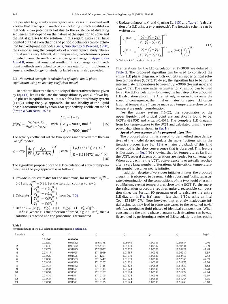
Details of the calculation of the liquid–vapor equilibrium forhe binary system CO2 + n-hexane at 393.15 K and 40 bar are givenn Table 6. Repeating this procedure at different pressures whileolding the temperature constant allows generating the completeuid phase diagram at 393.15 K, as shown in Fig. 4(a). Note thathis diagram culminates in a liquid–vapor critical point. More pre-isely, the phase diagram is constructed simply by solving thehase equilibrium equations at gradually increasing pressures. Thenly difficulty is found in the vicinity of the critical point: at P > Pc

where Pc denotes the critical pressure of the mixture), no phasequilibrium exists and the algorithm finds a trivial solution; at

< Pc, the solution of the phase-equilibrium problem is easily foundegardless of the initial estimates for the mole fractions x1 and y1.owever, the nearer the pressure is to the critical pressure, theloser are the compositions of both the equilibrium phases. There-ore, the following procedure is recommended for obtaining a phaseiagram that accurately captures the critical region:

Specify T and set P to Pinit (e.g. Pinit = 1 bar).Specify the pressure step, e.g. �P = 1 bar.

Set the initial values: k = 0, x(k)1 = 0.01 and y(k)

1 = 0.99. Solve the VLE problem at the current values of T and P usingthe algorithm presented above. A tolerance of � = 10−10 is rec-ommended.

If |x1 − y1| > �′ (e.g. �′ = 10−5), then a non-trivial solutionis found which is acceptable. A new value of P is specified suchthat P = P + �P; return to step 3.Else, a trivial solution is found which is rejected: the currentpressure is thus above the critical pressure. The pressure is thendecreased to the pressure of the last successful VLE calculation:P = P − �P. The pressure is then increased again with a smallerstep: �P = �P/10 and P = P + �P.

If �P < �Pmin (e.g. �Pmin = 10−4 bar), then the procedureis terminated;

Else, return to step 3.

Note that the values chosen for �, �′ and �Pmin are all inter-elated and must be adjusted depending on the case study under

able 6teration details of the VLE calculation performed in Section 3.5.

Iteration k x1 y1

0.01000 0.990001 0.19632 0.86966

2 0.21851 0.84785

3 0.22219 0.84312

4 0.22285 0.84206

5 0.22296 0.84182

6 0.22298 0.84177

7 0.22299 0.84175

8 0.22299 0.84175

9 0.22299 0.84175

10 0.22299 0.84175

l Engineering 50 (2013) 139– 151

consideration. The proposed values are the ones that were used tocalculate the phase diagram shown in Fig. 4(a).

Fig. 4(b) shows that few iterations are needed for calculations farfrom the critical point whereas the number of iterations approachesinfinity in the vicinity of the critical point. As previously noted, theproposed algorithm easily calculates fictitious equilibria character-ized by mole fractions greater than one or less than zero in domainsof temperatures and pressures when the binary system is in a sin-gle phase. In addition, the minimum number of iterations is foundat the pure-component VLE point.

Mathematical details on the convergence of two-dimensionaldirect-substitution methods can be found in Appendix B.

4. Derivation of a new algorithm for phase-equilibriumcalculation in ternary systems at a fixed temperature andpressure

4.1. General solution procedure

Following Eq. (8), the general form of the phase equilibriumrelations in a ternary system may be written as follows:

x′iF

′i = x

′′i F

′′i , ∀i ∈ �1; 3� (29)

The form of the Fi functions depends on the selected approach (�–ϕor ϕ–ϕ) and sometimes (as for the �–ϕ approach) on the nature ofthe phase equilibrium (VLE or LLE) involved, as shown in Table 1.At a fixed temperature and pressure, four variables are associatedwith the two-phase equilibrium problem: x′

1, x′2, x

′′1 and x

′′2; note that

the two remaining composition variables, x′3 and x

′′3, are not consid-

ered since they can be directly obtained from the two summationrelationships: x′

3 = 1 − x′1 − x′

2 and x′′3 = 1 − x

′′1 − x

′′2. In summary,

at fixed T and P, there are three phase-equilibrium equations andfour variables, leaving one degree of freedom. One variable amongthe four must be specified to solve the problem, with the threeremaining variables making up the set of unknowns. The phaseequilibrium problem in ternary systems at a fixed temperature andpressure then involves solving the following set of four equationswith respect to the four aforementioned unknowns:⎧⎪⎪⎪⎪⎨⎪⎪⎪⎪⎩

x′1F ′

1 = x′′1F

′′1

x′2F ′

2 = x′′2F

′′2

(1 − x′1 − x′

2)F ′3 = (1 − x

′′1 − x

′′2)F

′′3

Specification equation

(30)

The specification equation may apply to any of the six compositionvariables, e.g. x′

1 = s (where s denotes the value of the specified vari-′′ ′ ′ ′

able), or x2 = s, or x3 = s ⇔ 1 − x1 − x2 = s. As in binary systems, the

system of Eq. (30) can be equivalently expressed by matrix notationin the following form:

A X = B (31)

vL/(dm3 mol−1) vG/(dm3 mol−1) log ı

0.14930 0.74349 −0.020.13997 0.70000 −0.940.13917 0.68982 −1.690.13905 0.68751 −2.410.13903 0.68699 −3.110.13902 0.68687 −3.810.13902 0.68685 −4.500.13902 0.68684 −5.190.13902 0.68684 −5.870.13902 0.68684 −6.55

R. Privat et al. / Computers and Chemical Engineering 50 (2013) 139– 151 147

F T = 39r rgence

w

X

Tos

A

Oe

A

Adpcaf⎛⎜⎜⎜⎜⎝︸4u

T

)

ig. 4. (a) Isothermal phase diagram of the CO2 (1) + n-hexane (2) system plotted atespect to the number of iterations that are necessary to reach convergence (conve

here X represents the vector of unknowns:

=

⎛⎜⎜⎜⎜⎝

x′1

x′2

x′′1

x′′2

⎞⎟⎟⎟⎟⎠ (32)

he last line of the matrix A and the vector B depends on the choicef the specification equation. For instance, choosing x′

2 = s as apecification equation, one obtains:

=

⎛⎜⎜⎜⎜⎝

F ′1 0 −F

′′1 0

0 F ′2 0 −F

′′2

−F ′3 −F ′

3 F′′3 F

′′3

0 1 0 0

⎞⎟⎟⎟⎟⎠ and B =

⎛⎜⎜⎝

0

0

F′′3 − F ′

3

s

⎞⎟⎟⎠ (33)

therwise, choosing x′′3 = s ⇔ x

′′1 + x

′′2 = 1 − s as a specification

quation produces:

=

⎛⎜⎜⎜⎜⎝

F ′1 0 −F

′′1 0

0 F ′2 0 −F

′′2

−F ′3 −F ′

3 F′′3 F

′′3

0 0 1 1

⎞⎟⎟⎟⎟⎠ and B =

⎛⎜⎜⎝

0

0

F′′3 − F ′

3

1 − s

⎞⎟⎟⎠ (34)

n iterative scheme can be deduced from Eq. (31) similar to thateveloped for binary systems, by solving the phase equilibriumroblem for ternary systems at a fixed T, P for a given value of oneomposition variable. The mole fraction values at iteration (k + 1)re thus deduced from the mole fraction values at iteration k asollows:

x′1

x′2

x′′1

x′′2

⎞⎟⎟⎟⎟⎠

(k+1)

︷︷ ︸X(k+1)

=[A(X(k))

]−1B(X(k)) (35)

.2. Calculation of isothermal isobaric ternary phase diagrams

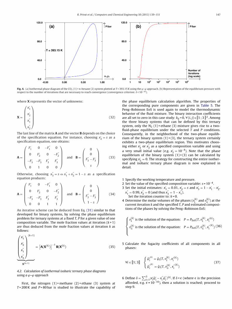
sing a ϕ–ϕ approach

First, the nitrogen (1) + methane (2) + ethane (3) system at = 200 K and P = 80 bar is studied to illustrate the capability of

3.15 K using the ϕ–ϕ approach. (b) Representation of the equilibrium pressure with criterion: ı < 10−10).

the phase equilibrium calculation algorithm. The properties ofthe corresponding pure components are given in Table 5. ThePeng–Robinson EoS is used again to model the thermodynamicbehavior of the fluid mixture. The binary interaction coefficientsare all set to zero in this case study: kij = 0, ∀ (i, j) ∈ �1 ; 3 � 2. Amongthe three binary systems that can be defined by this ternarysystem, only the N2 (1) + ethane (3) mixture gives rise to a two-fluid-phase equilibrium under the selected T and P conditions.Consequently, in the neighborhood of the two-phase equilib-rium of the binary system (1) + (3), the ternary system certainlyexhibits a two-phase equilibrium region. This motivates choos-ing either x′

2 or x′′2 as a specified composition variable and using

a very small initial value (e.g. x′2 = 10−4). Note that the phase

equilibrium of the binary system (1) + (3) can be calculated byspecifying x′

2 = 0. The strategy for constructing the entire isother-mal and isobaric ternary phase diagram is now explained indetail.

1 Specify the working temperature and pressure.2 Set the value of the specified composition variable: s = 10−4.3 Set the initial estimates: x′

1 = 0.01, x′2 = s and x′

3 = 1 − x′1 − x′

2.x

′′1 = 0.99, x

′′2 = 0 (and thus x

′′3 = 1 − x

′′1).

Set the iteration counter to: k = 0.4 Determine the molar volumes of the phases (v(k)

L and v(k)G ) at the

current iteration k and the specified T, P and estimated composi-tions of the phases by solving the Peng–Robinson EoS:

⎧⎪⎪⎨⎪⎪⎩

v(k)L is the solution of the equation: P = PEoS(T, v(k)

L , x′i(k))

v(k)G is the solution of the equation: P = PEoS(T, v(k)

G , x′′i

(k)) (36

5 Calculate the fugacity coefficients of all components in allphases:

∀i ∈ �1; 3�

{ϕ′(k)

i= ϕi(T, v(k)

L , x′i(k))

ϕ′′(k)

i= ϕi(T, v(k)

G , x′′i

(k))

(37)

6 Define ı =∑3

i=1|x′iϕ′

i− x

′′iϕ

′′i|(k). If ı < � (where � is the precision

afforded, e.g. � = 10−10), then a solution is reached; proceed tostep 9.

148 R. Privat et al. / Computers and Chemical Engineering 50 (2013) 139– 151

F ane (2a n of th

7

8

9

Fl

ig. 5. Left hand side: fluid phase behavior of the ternary system nitrogen (1) + methre tie lines. Right hand side: representation of the number of iterations as a functio

Calculate the matrix A and the vector B at the current iterationk:

A(k) =

⎛⎜⎜⎜⎜⎝

ϕ′1 0 − ϕ

′′1 0

0 ϕ′2 0 − ϕ

′′2

− ϕ′3 − ϕ′

3 ϕ′′3 ϕ

′′3

0 1 0 0

⎞⎟⎟⎟⎟⎠

(k)

and B(k) =

⎛⎜⎜⎝

0

0

ϕ′′3 − ϕ′

3

s

⎞⎟⎟⎠

(k)

(38)

Update the unknowns x′iand x

′′i

using Eq. (35). Note that the 4 × 4matrix A can be inverted using the so-called LU decompositionmethod, for instance. Proceed to step 4.

Increase the value for the specified variable: s = s + �s (e.g.�s = 10−3) and return to step 4.

If x′i

> 1 or x′i

< 0 or x′′i

> 1 or x′′i

< 0 (∀i∈ �1 ; 3 �), then the phasediagram is complete and the procedure is terminated.

If a critical point arises in the phase diagram (which is the casefor the N2 + methane + ethane system at 200 K and 80 bar), thentrivial solutions may be obtained. These trivial solutions are dealtwith exactly as for the binary systems (see Sections 3.3 and 3.5).

ig. 6. Left hand side: fluid phase behavior of the ternary system carbon dioxide (1) + propines are tie lines. Right hand side: representation of the number of iterations as a function

) + ethane (3) at 200 K and 80 bar represented in a triangular diagram. Dashed linese specified variable x′

2.

The left hand side of Fig. 5 shows the fluid-phase behavior of theaforementioned system in a triangular diagram calculated usingthe algorithm above. The shape of a liquid–liquid phase diagramis observed, culminating in a liquid–liquid critical point. The righthand side of Fig. 5 shows the number of iterations required for eachphase-equilibrium calculation, plotted as a function of the specifiedvariable x′

2. This number is once more observed to approach infinityin the vicinity of the critical point.

As another illustration, Fig. 6 shows the phase diagram of theternary system CO2 (1) + propane (2) + ethane (3) at 230 K and11 bar calculated using the Peng–Robinson EoS. Binary interac-tion coefficients were considered for CO2 + alkane binary mixtures:kCO2/alkane = 0.15.

For this system and because of the banana shape of thetwo-phase region, the most convenient variables to specify areeither x3 or y3. The variable y3 was chosen for the presentcase and fixed at s = 0.237 for the first ternary phase equilib-rium calculation (note that this value was deduced from thecalculation of the two-phase equilibrium of the binary system

(1) + (3) at 230 K and 11 bar). The matrix A is then given by Eq.(34). The ‘Iteration number’ versus y3 diagram given in Fig. 6shows that several dozen iterations are systematically needed forconvergence.

ane (2) + ethane (3) at 230 K and 11 bar represented in a triangular diagram. Dashed of the specified variable y3.

emical Engineering 50 (2013) 139– 151 149

5

calvptv

acogata

ptn

rbawtsfe

pporr&p

Amu

A

3p

q

ttbcfimrtap

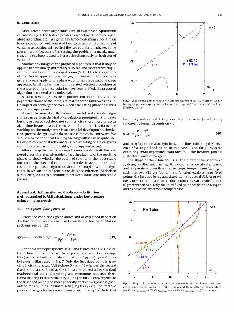
Fig. 7. Shape of the q function for a non-azeotropic system at t = 63 ◦C and P = 1.5 bar,

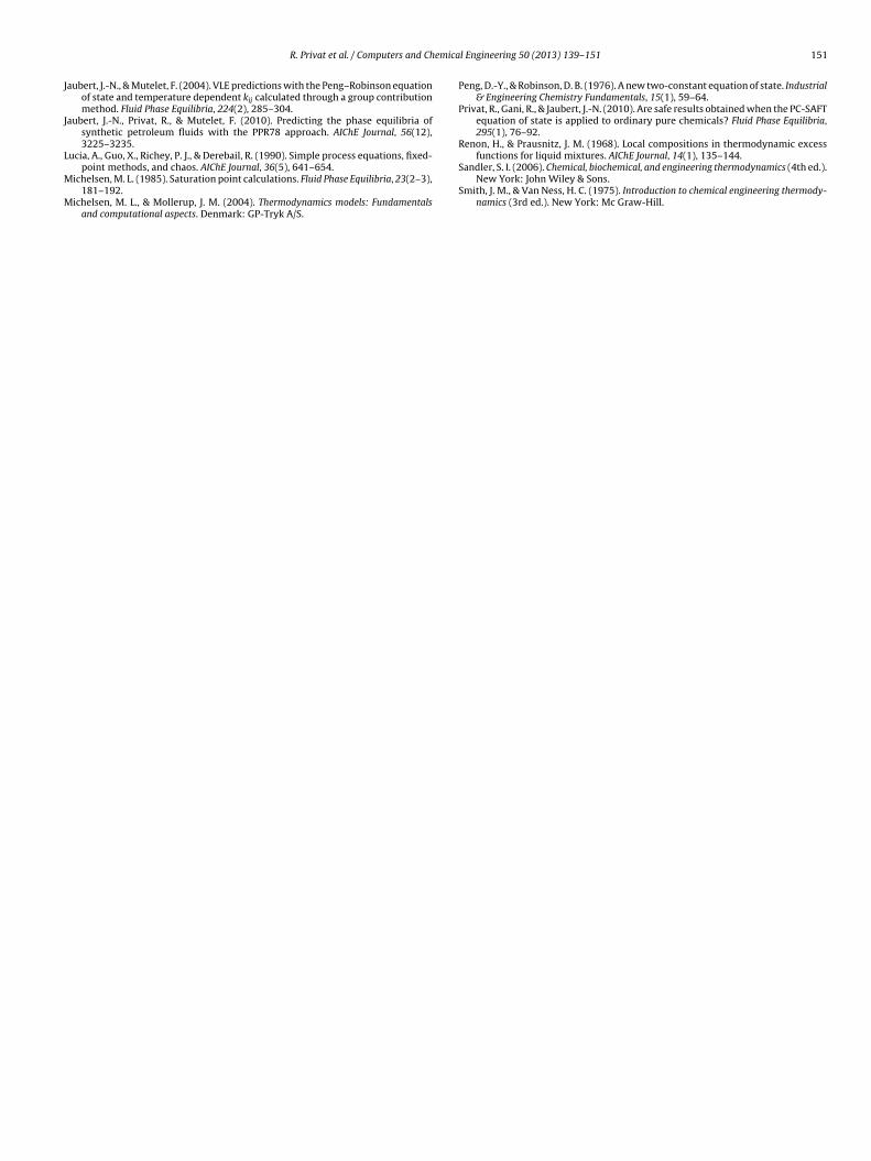
x* greater than one. Only the third fixed point persists at a temper-ature above the azeotropic temperature.

R. Privat et al. / Computers and Ch

. Conclusion

Most zeroth-order algorithms used in two-phase equilibriumalculations (e.g. the bubble pressure algorithm, the dew temper-ture algorithm, etc.) are generally time-consuming since a mainoop is combined with a nested loop to iterate on the two sets ofariables associated with each of the two equilibrium phases. In theresent work, because of re-casting the problem in matrix nota-ion, only one loop is used to iterate simultaneously on both sets ofariables.

Another advantage of the proposed algorithm is that it may bepplied to both binary and ternary systems, and more interestingly,an treat any kind of phase equilibrium (VLE, LLE, etc.) regardlessf the chosen approach (ϕ–ϕ or �–ϕ) whereas other algorithmsenerally only apply to one phase-equilibrium type and one givenpproach. As all the formalisms and related solution procedures inhe phase-equilibrium calculation have been unified, the proposedlgorithm is claimed to be universal.

A third advantage has been pointed out in the body of theaper: the choice of the initial estimates for the unknowns has lit-le impact on convergence even when calculating phase equilibriaear azeotropic points.

It could be remarked that more powerful and complex algo-ithms can perform the kind of calculations presented in this paperut the proposed tool does not conflict with these more complexlgorithms by any means. The current tool is appropriate for peopleorking on thermodynamic issues (model development, simula-

ion, process design...) who do not use commercial softwares. Wehould also mention that the proposed algorithm can be quite use-ul where commercial software fails in calculating phase diagramsxhibiting singularities (criticality, azeotropy and so on).

After solving the two-phase equilibrium problem with the pro-osed algorithm, it is advisable to test the stability of the resultinghases to check whether the obtained solution is the most stablene under the specified conditions. In order to avoid undesirableesults, the proposed algorithm should be coupled with an algo-ithm based on the tangent plane distance criterion (Michelsen

Mollerup, 2004) to discriminate between stable and non-stablehases.

ppendix A. Information on the direct-substitutionethod applied to VLE calculations under low pressure

sing a �–ϕ approach

.1. Description of the q function

Under the conditions given above and as explained in Section.4, the VLE problem at a fixed T and P results in a direct-substitutionroblem (see Eq. (22)):

(x1) = x1 with : q(x1) = P − Psat2 �2

Psat1 �1 − Psat

2 �2(39)

For non-azeotropic systems at a T and P such that a VLE exists,he q function exhibits two fixed points and a vertical asymp-ote (associated with a null denominator: Psat

1 �1 − Psat2 �2 = 0). This

ehavior is illustrated in Fig. 7. Only the first fixed point is asso-iated with the actual VLE (where 0 ≤ x1 ≤ 1) whereas the secondxed point can be found at x* > 1. It can be proved using standardathematical tools (alternating and monotone sequence theo-

ems) that any initial estimate x1 ∈ [0 ; 1] results in convergence tohe first fixed point (and more generally, that convergence is guar-nteed for any initial estimate satisfying 0 < x1 < x*). The iterativerocess diverges for an initial estimate such that x1 > x*. Note that

having the properties presented in Section 3.4 excepted Psat1 = 3 bar and Psat

2 = 1 bar.(©) fixed points.

for binary systems exhibiting ideal liquid behavior (� i = 1), the qfunction no longer depends on x1:

q(x1) = P − Psat2

Psat1 − Psat

2

(40)

and the q function is a straight horizontal line, indicating the exist-ence of a single fixed point. In this case – and for all systemsexhibiting small departures from ideality – the iterative processis strictly always convergent.

The shape of the q function is a little different for azeotropicsystems, as illustrated in Fig. 8. Indeed, at a specified pressureand temperature lower than the azeotropic temperature (tazeotrope),such that two VLE are found, the q function exhibits three fixedpoints, the first two being associated with the actual VLE. As previ-ously mentioned, an additional fixed point exists at a mole fraction

Fig. 8. Shape of the q function for an azeotropic system having the prop-erties presented in Section 3.4, at P = 1 atm and three different temperatures(t = 63 ◦C < tazeotrope, t = 65 ◦C < tazeotrope and t = 66 ◦C > tazeotrope). (©) fixed points.

150 R. Privat et al. / Computers and Chemical Engineering 50 (2013) 139– 151

Fig. 9. Derivative of the q function for an azeotropic system at P = 1 atm andt = 63 ◦C < tazeotrope, having the properties presented in Section 3.4. (©) fixed points.

A

gq

•

•

References

.2. On the convergence and divergence of iterative processes

Let us recall that essentially two factors impact the conver-ence of a fixed-point algorithm for solving an equation of the type(x1) = x1:

the value of the derivative |q′(xfp)|, where xfp is the coordinate ofthe fixed point. Then,– if |q′(xfp)| < 1, the fixed-point method will converge to the fixed

point with coordinates (xfp, xfp) assuming an appropriate initialestimate for x1. The fixed point is then called attractive.

– if |q′(xfp)| > 1, the fixed-point method will diverge. The corre-sponding fixed point is called repulsive.

– if |q′(xfp)| = 1, the fixed-point iterative process will be eitherdivergent or convergent (more detailed analysis is needed todraw a conclusion).Fig. 9 illustrates this instance. The first two fixed points are

associated with a derivative |q′(xfp)| < 1 and are thus attractive.The third fixed point is associated with a derivative q′(xfp) > 1 andis thus repulsive.the quality of the initial estimate.

For |q′(xfp)| < 1, the fixed-point method converges in the vicinityof the fixed point. It thus becomes possible to define a basin ofattraction that contains all the initial estimate values that lead toa converging iterative process.

The sensitivity of the fixed-point method with respect to theinitial estimates was discussed in Section 3.4 and illustrated inFig. 3 where the basins of attraction (i.e. the domains of conver-gence) are shown. At a fixed T and P such that two VLE exist, oneobserves that a domain of divergence (denoted by [xlim,1, xlim,2]) inthe composition range [0 ; 1], systematically exists (i.e. any initialvalue of x1 within this domain will cause the fixed-point methodto diverge).

Graphical construction shows that for any x1 ∈ [xlim,1, xlim,2],the fixed-point method almost immediately produces x1 valuesgreater than x*, the coordinate of the repulsive fixed point, thusexplaining the diverging process. By using the borderline valuesxlim,1 and xlim,2 as initial estimates, the fixed-point method con-verges exactly to the repulsive fixed point (x*, x*), as shown in

Fig. 10.

Fig. 10. Illustration that the fixed-point method initialized to xlim,1 or xlim,2, con-verges to the repulsive fixed point (x*, x*), for an azeotropic system at P = 1 atm andt = 63 ◦C < tazeotrope, having the properties presented in Section 3.4. (©) fixed points.

Appendix B. On the convergence of the direct-substitutionmethod as applied to two-dimensional problems

This section shows how the conclusions presented in AppendixA (which dealt with the convergence of the one-dimensional direct-substitution method) can be generalized to two-dimensionalproblems.

As shown in the body of the paper, the two-phase equilibriumproblem for binary systems at fixed temperature and pressure, canbe expressed by the following general form:{

q1(X) = X1

q2(X) = X2(41)

with X1 = x′1, the mole fraction of component 1 in one phase, and

X2 = x′′1 the mole fraction of component 1 in the other phase.

Let us denote a fixed point by Xfp and the Jacobian matrix asso-ciated with the q function by q′

ij= ∂qi/∂Xj . The two eigenvalues of

q′ are denoted �1 and �2 (�i ∈ C); they are not necessarily distinct.The convergence of the two-dimensional direct-substitution

process obeys the following rules:

• if q′(Xfp) has at least one eigenvalue satisfying |�i| > 1, initial esti-mates can be found that are arbitrarily close to the fixed pointsuch that the method is divergent.

• if all the eigenvalues of q′(Xfp) satisfy |�i| < 1, an open set con-taining Xfp exists such that any initial estimate chosen withinthis open set makes the method convergent.

• if there is one eigenvalue such that |�i| = 1 (and the other eigen-value satisfies |�i| ≤ 1) then the iterative process will be eitherdivergent or convergent (and more detailed analysis is needed todraw a conclusion).

Remark: the convergence of the direct-substitution method canbe accelerated by using Aitken’s delta-squared process, for instance.

Deiters, U. K. (2002). Calculation of densities from cubic equations of state. AIChEJournal, 48(4), 882–886.

emica

J

J

L

M

M

functions for liquid mixtures. AIChE Journal, 14(1), 135–144.

R. Privat et al. / Computers and Ch

aubert, J.-N., & Mutelet, F. (2004). VLE predictions with the Peng–Robinson equationof state and temperature dependent kij calculated through a group contributionmethod. Fluid Phase Equilibria, 224(2), 285–304.

aubert, J.-N., Privat, R., & Mutelet, F. (2010). Predicting the phase equilibria ofsynthetic petroleum fluids with the PPR78 approach. AIChE Journal, 56(12),3225–3235.

ucia, A., Guo, X., Richey, P. J., & Derebail, R. (1990). Simple process equations, fixed-

point methods, and chaos. AIChE Journal, 36(5), 641–654.

ichelsen, M. L. (1985). Saturation point calculations. Fluid Phase Equilibria, 23(2–3),181–192.

ichelsen, M. L., & Mollerup, J. M. (2004). Thermodynamics models: Fundamentalsand computational aspects. Denmark: GP-Tryk A/S.

l Engineering 50 (2013) 139– 151 151

Peng, D.-Y., & Robinson, D. B. (1976). A new two-constant equation of state. Industrial& Engineering Chemistry Fundamentals, 15(1), 59–64.

Privat, R., Gani, R., & Jaubert, J.-N. (2010). Are safe results obtained when the PC-SAFTequation of state is applied to ordinary pure chemicals? Fluid Phase Equilibria,295(1), 76–92.

Renon, H., & Prausnitz, J. M. (1968). Local compositions in thermodynamic excess

Sandler, S. I. (2006). Chemical, biochemical, and engineering thermodynamics (4th ed.).New York: John Wiley & Sons.

Smith, J. M., & Van Ness, H. C. (1975). Introduction to chemical engineering thermody-namics (3rd ed.). New York: Mc Graw-Hill.