Computers & Industrial Engineering

Contents lists available at ScienceDirect

Computers & Industrial Engineering

journal homepage: www.elsevier.com/locate/caie

A Branch-and-Cut algorithm for the Capacitated Multi-Failure SurvivableNetwork Design problem

S. Bornea, E. Gourdinb, O. Klopfensteinc, A.R. Mahjoubd,⁎

a Laboratoire LIPN, UMR CNRS 7030, Universit_e Paris 13, Sorbonne Paris Cité, 99 Avenue J-B. Clément, 93430 Villetaneuse, FrancebOrange Labs, 44 avenue de la République CS 50010, 92326 Chatillon Cedex Francec EDF – R&D, 1 av. du Général de Gaulle, 92141 Clamart, FrancedUniversité Paris-Dauphine, PSL Research University, CNRS, UMR [7243], LAMSADE, Place du Maréchal de Lattre de Tassigny, 75775 Paris Cedex 16, France

A R T I C L E I N F O

Keywords:IP-over-optical networkSurvivabilityCapacitiesPolytopeFacetBranch-and-Cut-and-Price algorithms

A B S T R A C T

Telecommunication networks can be seen as the stacking of several layers like, for instance, IP-over-Opticalnetworks. This infrastructure should have sufficient capacities to route some demands between their origin-destination nodes. In this paper we consider the Capacitated Multi-Failure Survivable Network Design problem.We study two variants of this problem with simple and multiple capacities. We give two multicommodity flowformulations for each variant of this problem and describe some valid inequalities. In particular, we characterizevalid inequalities obtained using Chvatal-Gomory procedure from the well known Cutset inequalities. We showthat some of these inequalities are facet defining. We discuss separation routines for all the valid inequalities.Using these results, we develop a Branch-and-Cut algorithm and a Branch-and-Cut-and-Price algorithm for eachvariant and present extensive computational results.

1. Introduction

In the past years, telecommunication networks have seen an im-portant development with the advances in optical technologies and theexplosive growth of the Internet. Also the data traffic has increaseddramatically and has now surpassed voice traffic in volume. Using thenew optical technologies, different systems allow a very large increaseof data transportation capacity and the transfer of almost illimitatedquantities of information. Hence, in the event of a failure, a big amountof traffic may be lost. As a consequence, telecommunication networksmust have a survivable topology, that is to say a configuration of theirnodes and the links between the nodes that permits the communicationto be restored and the network to remain functional in the event of afailure. For this, network survivability has become a major objective inthe design of telecommunication networks.

Data networks have always been analyzed, described and managedin a multilayer structure. Indeed, it is quite natural to assume that themore elaborate functionalities of a network rely on a set of simple onesprovided by some lower layer. This is in particular the case of moderntelecommunication networks where different technologies (SDH/SONET, WDM, Gigabit Ethernet, IP, …) are combined in various wayson successive layers. From a practical point of view, this means that, inorder to carry its traffic on some layer, the network may need to use a

lower-level technology. Then several layers can be piled up in order tohave an operational network offering a variety of services. The ad-vantage of this is that each technology can be used for its most favor-able features. Moreover, each technology is characterized by a certainrange of traffic rates. The drawback, however, is that each technology,and hence each layer, manages its own routing control scheme in-dependently from the others, and addresses its own survivability issues.Ghani et al. (2008) present a survey of the various new and hetero-geneous infrastructures in telecommunication networks and address thechallenges on these new technologies in the area of survivability. InPacharintanakul and Tipper (2009), Pacharintanakul and Tipper in-vestigate survivability strategies for IP-over-WDM networks in a mul-tilayer framework where traffic originates at each layer. They presentoptimization models and experimental results using Cplex.

The capacities of a given layer correspond to the (worst-case) trafficdemands that must be routed on the layer just below. The process ofdetermining the capacities to install on the different layers of a net-work, usually called dimensioning, often reduces to a succession ofmulticommodity flow problems (A multicommodity flow is a super-position of different flows between origine-destination pairs). Usuallythere is an empirical relation between these problems, and the wholedimensioning problem is never treated in an optimal way. As a con-sequence, in a network design problem, reliability is considered layer

https://doi.org/10.1016/j.cie.2018.05.043

⁎ Corresponding author.E-mail address: [email protected] (A.R. Mahjoub).

Computers & Industrial Engineering 124 (2018) 582–603

Available online 30 May 20180360-8352/ © 2018 Elsevier Ltd. All rights reserved.

T

http://www.sciencedirect.com/science/journal/03608352

https://www.elsevier.com/locate/caie



mailto:[email protected]


http://crossmark.crossref.org/dialog/?doi=10.1016/j.cie.2018.05.043&domain=pdf

by layer without tackling the redundancy and the non-optimalityyielded by the multilayer structure. Moreover, a failure in the networkcan be handled by several successive layers. This results in a potentialhuge global over-provisioning of resources, each layer protecting inturn the ones above. However the relation between technologies used inthe different layers is usually complex, and does not permit to effi-ciently correlate the control of the successive layers. In consequence,the solution provided for this multilayer survivability problem usuallyconsists of an over protection of the whole network. But this may bevery costly and sometimes not efficient.

The introduction of new protocols in telecommunication (like MPLSand GMPLS) (Zouganeli, 2001) gives a new trend for multilayer datanetworks. These new systems provide a common signaling and routingframework between the different layers, and they do not restrict theway these layers work together. This evolution is yielding new survi-vability issues in multilayer networks. In Voge (2006), Voge studiesdifferent problems about the multilayer telecommunication networksbased on MPLS and GMPLS. Bigos, Cousin, Gosselin, Foll, and Nakajima(2007) study different options for the survivability implementation inMPLS over Optical Transport Networks. They give an integer linearprogramming formulation for the underlaying optimization problem.

In this paper we introduce a multilayer capacitated survivablenetwork design problem that may be of practical interest for the designand the dimensioning of IP-over-optical networks. These networks,based on the GMPLS technology, consist of two layers, the IP (client)layer and the optical (transport) layer. The two layers are representedby two graphs G1 and G2, respectively. If a link e in the optical networkis cut, a set of edges Fe of the IP network may be affected. We supposethat a set of traffic demands must be routed in the IP network betweensome origin-destination pairs. We also suppose that two types of ca-pacities can be installed in the IP network in order to route the de-mands. If a cost is associated with each type of capacity, the problem isto determine the minimum cost set of capacities to be installed in the IPnetwork so that the traffic demands can be routed in the event of anyfailure in the IP network, that is to say in any subgraph ⧹G Fe1 obtainedfrom G1, by deleting Fe, for all edge e of G2. We provide mixed integerprogramming formulations for this problem and discuss Branch-and-Cut and Branch-and-Cut-and-Price algorithms.

Survivability and dimensioning have already been studied in theliterature for multilayer networks. In particular, heuristic approacheshave been proposed. In Gouveia, Patrício, de Sousa, and Valadas (2003)and Gouveia, Patrício, and de Sousa (2008), Gouveia and Patrício studythe design of MPLS-over-WDM networks. They address the di-mensioning subject to some path constraints in the WDM layer and hopconstraints in the MPLS layer. They give an integer programming for-mulation and devise a heuristic technique based on that formulation. InRicciato, Salsano, Belmonte, and Listanti (2002), Ricciato et al. considerthe problem of off-line configuration of MPLS-over-WDM networksunder time-varying offered traffic. They present a mixed integer pro-gramming formulation for the problem and discuss heuristic ap-proaches. Binh and Ly (2012) propose a genetic algorithm for solving amultilayer survivable optical network design problem. A genetic basedalgorithm is also proposed by Ruiz et al. (2011) for survivable IP/MPLS-over-WSON multilayer network optimization. There are also some re-cent works carried out on two-layered network design with or withoutdimensioning. Orlowski and Wessäly (2004) describe a general integerlinear programming model for the design of multilayer tele-communication network design problem which integrates hardware,capacity, routing and grooming decisions. They give also a sketch of analgorithmic approach. Orlowski, Koster, Raak, and Wessäly (2006)develop three primal heuristics to be called in a Branch-and-Cut algo-rithm to solve the problem with two layers. Koster, Orlowski, Raack,Baier, and Engel (2008) consider a planning problem arising in SDH/WDM multilayer telecommunication network design. They present amixed-integer programming formulation and a Branch-and-Cut ap-proach with cutting planes based on either of the two layers. Knippel

and Lardeux (2007) study heuristic and exact algorithms based onmetric inequalities for a multilayer network design problem (see alsoLardeux, 2005). Mattia (2013) considers this problem from a poly-hedral point of view. She presents valid inequalities and describesconditions for theses inequalities to be facet defining. Fortz and Poss(2009) develop a Branch-and-Cut algorithm to solve the Benders de-composition of the problem. As a consequence, they improve the con-straints generation method used by Knippel and Lardeux (2007). Borne,Gabrel, Mahjoub, and Taktak (2011) study a survivability problem inmultilayer IP-over-optical networks. They formulate the problem interms of 0–1 linear program based on path variables and propose aBranch-and-Price algorithm.

The first major survivability requirement used in telecommunica-tion networks is the so-called 2-connectivity. That is there must exist atleast two edge-disjoint paths between every pair of nodes in the net-work. This implies that the network remains connected in the event ofany single edge failure. The problem of finding a minimum cost 2-edgeconnected subgraph has been extensively investigated in the past dec-ades (Barahona & Mahjoub, 1995; Grötschel, Monma, & Stoer, 1995;Kerivin, 2000; Kerivin & Mahjoub, 2005; Mahjoub, 1994; Stoer, 1992).

Dahl and Stoer (1998) present a cutting plane approach for solvingthe MULTIcommodity SUrvivable Network design problem (MULTISUNproblem). This consists, given point-to-point traffic demands in a net-work, in finding minimum cost capacities that permit the routing of thegiven demands. The possible capacity choices on each edge give rise toa discrete cost function. Another problem called the Network LoadingProblem (NLP) plays a central role in the design of telecommunicationnetworks. It is a special case of the MULTISUN problem. For the NLP, asingle type of capacitated facility is considered, and each link can beassigned one or several types of capacities in such a way that the net-work can carry given point-to-point demands at minimum cost.Barahona (1996) studies this problem in the both unsplittable andsplittable cases that is when the flow of each commodity is carried by asingle path or when it could use several paths. He proposes a separationalgorithm for the so-called cut inequalities, which seem to play a centralrole for solving the problem. In Magnanti, Mirchandani, and Vachani(1993) Magnanti et al. study the polyhedral structure of two coresubproblems of the NLP. And in Magnanti, Mirchandani, and Vachani(1995) they discuss a further problem, called the Two-Facility capaci-tated network Loading Problem (TFLP), in which two types of capa-cities are considered.

The paper is organized as follows. In the following section we dis-cuss the IP-over-optical networks and the interaction between the dif-ferent layers. We present a multilayer survivable network design pro-blem with capacity constraints, called the multilayer capacitatedsurvivable IP network design problem. We describe two versions of thisproblem: with and without multiple edges. We give mixed integerprogramming formulations for this problem. In Section 3, we study theassociated polytopes. We identify a few classes of valid inequalities anddescribe conditions for theses inequalities to be facet defining. In Sec-tion 4, we describe the Branch-and-Cut algorithms and Branch-and-Cut-and-Price algorithms for the problem. Our computational results arepresented and discussed in Section 5. In Section 6, we give some con-cluding remarks.

2. The Capacitated Multi-Failure Survivable Network DesignProblem

2.1. Multilayer telecommunication networks

Telecommunication networks are now moving toward a model ofhigh-speed routers interconnected by intelligent optical core networks.Moreover, there is a general consensus that the control plan of theoptical networks should utilize IP-based protocols for dynamic provi-sioning and restoration of lightpaths (Bradner, 1995; Jensen, 2001;Postel, 1981a, 1981b, 1981c).

S. Borne et al. Computers & Industrial Engineering 124 (2018) 582–603

583

The optical network consists of multiple switches (also calledOptical Cross-Connects (OXC)) interconnected by optical links. The IPand optical networks communicate through logical control interfacescalled User-Network-Interfaces (UNI). The optical network essentiallyprovides point-to-point connectivity between routers in the form offixed bandwidth paths called lightpaths. These lightpaths define thetopology (the structure of the network given by the nodes and thepossible links between the nodes) of the IP network.

Each router in the IP network is connected to at least one of theoptical switches. Moreover to each link between two routers in the IPnetwork corresponds a routing path in the optical one between twoswitches corresponding to these routers. This routing path is used forrouting the traffic between the two switches. The set of routing paths isalso referred to as the routing of the network. Fig. 1 shows an IP-over-optical network. The IP network has four routers …R R, ,1 4 and theoptical network has seven switches …S S, ,1 7. Only the optical switches

…S S, ,1 4 communicate with one router through the UNI.Using this infrastructure of telecommunication networks give rise to

survivability issues. For example consider the IP-over-optical networkgiven in Fig. 1. Suppose that the link −R R1 2 of the IP network corre-sponds to the optical path −S S1 2, and the link −R R1 3 corresponds to thepath − − −S S S S1 2 6 3. Here, the network is not survivable to single linkfailures. For instance, if the optical link −S S1 2 fails, then the links in theIP network −R R1 2 and −R R1 3 are cut, and therefore the router R1 is nomore connected to the rest of the routers. As a consequence, surviva-bility strategies have to be considered. If the transport network is fixed,one has to determine the suitable client network topology for the net-work to be survivable.

In addition to the survivability aspect, it is sometimes necessary toinstall capacities on the IP network in order to route commodities be-tween some routers. In this paper we shall discuss this problem whichconsiders simultaneously both the survivability and the dimensioningof the IP network when the transport network is fixed.

2.2. The problem

The first major survivability requirement used in telecommunica-tion networks is the 2-connectivity. That is there must exist at least twoedge-disjoint paths between every pair of nodes in the network. Thisassumption, that only one edge may fail at a time, is based on the naiveidea that the links in the network are independent and no equipmentcan be commonly used by two distinct links. However, this is not thecase, for instance, for the IP-over-optical networks, when the opticallayer is taken into account in the management of the IP network.

Indeed, an edge of the optical network may appear in several pathssupporting distinct edges. In consequence, the failure of an edge in theoptical network may affect several optical paths, and hence the edges ofthe client network corresponding to these paths. As a result, severaledges may fail at the same time in the IP layer (such a group of links is

usually referred to as a Shared Risk Link Group, or SRLG).The multilayer survivable IP network design problem (MSIPND

problem) introduced by Borne, Gourdin, Liau, and Mahjoub (2006)consists in finding the set of links to be installed in the IP network sothat if a failure occurs on an optical link, the IP subnetwork obtained byremoving the corresponding edges is connected.

In our problem, we can install capacities of 2.5 Gbits or 10 Gbits onany link of the IP network. Moreover, we consider that each time acertain capacity is installed from a router R1 to a router R2, one has toinstall the same capacity from R2 to R1.

Consequently, a more realistic model which has to be investigated,would consist in setting up capacities with a minimum cost to the clientnetwork that allows a multicommodity flow which satisfies the capa-cities for any simple edge failure in the transport network.

In this paper we consider this problem. More precisely, we considerthe overlay model where the IP and the optical networks are separated.We suppose that the topology and the routing of the optical network arefixed and satisfy some survivability requirements. Here the routing isthe way the traffic is routed in the network. It corresponds to a set ofpaths between the origin-destinations which carry the traffic. We alsosuppose that the optical network is already dimensioned and has en-ough capacity to convey the network traffic. So here, we will focus onthe management of the logical layer. We suppose that a set of IP routers(resp. optical switches) is given as well as the possible links between therouters (resp. switches). As the routing of the optical network is known,one can determine for each optical link e, the set of edges of the IPnetwork that may be affected if e is cut. We also suppose that sometraffic demands, also called commodities, have to be routed betweensome pairs of origin-destination nodes. Each demand is of a certainamount. If a certain cost is associated with each type of capacity oneach edge of the IP network, the Capacitated Multi-Failure SurvivableNetwork Design problem (SND-MF problem) is to find the minimum costset of links to be installed in the IP network and the capacities to beinstalled on these links so that if a failure occurs on an optical link, theIP subnetwork obtained by removing the corresponding edges allows arouting of the demands which satisfies the capacities. In the rest of thepaper we will also use the term facility to designate either the capacity2.5 Gbits or 10 Gbits that will be used in the network.

We consider two variants of the problem: the multiple SND-MF(denoted by SND-MFm) which allows multiple links, and the simpleSND-MF (denoted by SND-MFs) where only one link of one type ofcapacity can be loaded between two routers. Throughout the paper, ifno confusion, we will write SND-MF for the two problems SND-MFm andSND-MFs.

In what follows we give mixed integer programming formulationsfor the SND-MF problem. To this end, we first introduce some defini-tions and notations.

2.3. Definitions and notations

We consider undirected graphs. We denote a graph by =G V E( , )where V is the node set and E the edge set of G. If ∈e E is an edgebetween two nodes u and v, then we also write =e uv to denote e. Wedenote also by =D V A( , ) the bidirected graph associated with G suchthat each edge = ∈e uv E is replaced by two arcs u v( , ) and v u( , ), re-spectively from u to v and from v to u, in the arc set A of D. For an edgesubset ⊆F E we denote by

⎯→⎯⊆F A the associated arc subset. For ⊆F E

we let ⧹G F denote the subgraph of G obtained by removing the edges of

F and ⧹⎯→⎯

D F the associated subgraph obtain from D by removing the

arcs of⎯→⎯F . Throughout the paper we will consider simple graphs.

Let =G V E( , ) be a graph. For ⊆W V , we denote by G W( ) thesubgraph of G induced byW that is the subgraph havingW as a node setand all the edges whose both endnodes are in W. If ⊂W V W, denotes⧹V W . If U and W are two node subsets such that ∩ = ∅U W , then we

denote by U W[ , ] the set of edges having one node in U and the other in

Fig. 1. An IP-over-optical network.


584

W. If …V V, , p1 is a partition of V, we let …δ V V( , , )G p1 denote the set ofedges of G between the elements of the partition. If =p 2 and =V W1 ,we write δ W( )G for δ V V( , )G 1 2 . In this case δ W( )G is called a cut.

Given a graph =G V E( , ), a path P in =G V E( , ) is an alternatesequence of nodes and edges … +v e v e v e v( , , , , , , , )p p p1 1 2 2 1 such that= +e v vi i i 1 for = …i p1, , and ≠v vi j for = … + = … +i p j p1, , 1, 1, , 1.

Nodes +v v, p1 1 are the endpoints of P and we will say that P goes from v1to +vp 1 or P is between v1 and +vp 1.

Given a vector ∈x IRE and ⊆F E , we let = ∑ ∈x F x e( ) ( )e F .Throughout the paper, given an IP-over-optical network, we sup-

pose that to each router of the IP layer corresponds exactly one opticalswitch. We will represent an IP-over-optical network by two graphs

=G V E( , )1 1 1 and =G V E( , )2 2 2 , that represent the IP and optical net-works, respectively. The nodes of G1 (resp. G2) correspond to the routersof the IP layer (resp. the optical switches), and the edges represent thepossible links between the routers (resp. switches). A vertex ∈w Vi

2 isassociated with a vertex ∈v Vi

1. For an edge ∈f E1, we denote by Pf thepath in G2 corresponding to f. Fig. 2 shows graphs G1 and G2 corre-sponding to the IP-over-optical network of Fig. 1. In G2, are indicatedtwo paths Pe and Pf which correspond to the edges e and f of G1.

2.4. Formulations

In terms of graphs, the SND-MF problem can be presented as fol-lows.

For an edge e of graph =G V E( , )2 2 2 corresponding to the opticalnetwork, let ***Fe be the set of edges of the IP network that may beaffected by a failure of e, that is = ∈ ∈F f E e P{ | }e f

1 . We let� = ∈F e E{ , }e

2 . Also we denote by D1 the directed graph associated

with G1 and � �⎯→⎯

=⎯→⎯

∈F F{ | }e e . We denote by K the set of commodities.For each commodity ∈k K , we know the origin ok, the destination dkand the amount ωk of the demand k.

Let = =μ μ 2.51 Gbit/s and = =μ μ4 102 Gbit/s be the possiblecapacities. For each ∈ij E1, let cij

l be the cost of installing a capacity μl

on ij for =l 1, 2. Then, the SND-MFm problem consists in finding aminimum cost subgraph H of G1 such that for every edge ∈e E2, thegraph obtained from H by removing the edges of Fe has enough capacityto route the commodities of K with respect to the capacity of the re-maining edges.

In what follows we give two different formulations for the SND-MFproblem: the node-arc or conventional formulation and the path orcolumn-generation formulation.

2.4.1. Node-arc formulationIn order to give a node-arc formulation for the SND-MF problem, let

us denote by fuvk e, the value of the flow of commodity ∈k K on arc

∈u v A( , ) 1, in case of failure of edge ∈e E2 (i.e., when the arcs of⎯→⎯Fe are

removed in D1). For an edge ∈uv E1, let xuvl be the number of facilities

μl installed on uv, for =l 1, 2. Set

=⎧

⎨⎩

− =≠=

∈ ∈bω v o

v o dω v d

v V k Kif ,

0 if , ,if ,

for all , for all .kv

k k

k k

k k

1

Hence the multiple SND-MF problem is equivalent to the followinginteger programming problem.

Minimize ∑ ∑= ∈ c xl uv E uvl

uvl

1,2 1

∑ ∑− = ∈ ∈∈∈ ⧹

⎯→⎯∈ ⧹

⎯→⎯f f b v V k K

e Efor all , for all ,for all ,u u v A F

uvk e

u v u A Fvuk e

kv

:( , )

,

:( , )

, 1

2e e

1 1

(1)

∑ ⩽ + ∈∈∈

f μ x μ x uv Ee E

for all ,for all ,k K

uvk e

uv uv, 1 1 2 2 1

2 (2)

∑ ⩽ + ∈∈∈

f μ x μ x uv Ee E

for all ,for all ,k K

vuk e

uv uv, 1 1 2 2 1

2 (3)

⩾ ∈ =x uv E l0and integerfor all , 1, 2,uvl 1 (4)

⩾ ∈∈ ∈

f f uv Ek K e E

, 0 for all ,for all , for all .uv

k evuk e, ,

1

2 (5)

Inequalities (1) are called flow conservation constraints. Inequalities(2) and (3) express the fact that the sum of the flows of all commodities∈k K on an edge has to be less than or equal to the capacity of this

edge. They will be called capacity constraints. Inequalities (4) and (5)are called trivial inequalities.

By adding the following inequalities

+ ⩽ ∈x x uv E1 for all ,uv uv1 2 1 (6)

and by replacing inequalities (4) by

∈ ∈ =x uv E l{0, 1} for all , 1, 2,uvl 1 (7)

we obtain a valid formulation for the simple SND-MF problem.Inequalities (6) express the fact that only one link can be used be-

tween two given nodes. Then we have only one type of capacity on anedge. Constraints (7) are the integrality constraints that express the factthat =x 1uv

l if capacity =μ l, 1, 2l , is installed on uv and 0 otherwise.Note that the following inequalities

+ ⩽ ∈ ∈ ∈f f ω uv E k K e Efor all , for all , for all ,uvk e

vuk e

k, , 1 2

(8)

are valid for the SND-MF problem. They are called bound inequalities.

2.4.2. Path formulationAs in the node-arc formulation, for an edge ∈uv E1 we denote by xuv

l

the number of facilities μl installed on uv for =l 1, 2. For an edge ∈e E2

and a commodity k we denote by � ke the set of paths from ok to dk in the

graph ⧹⎯→⎯

D Fe1 (i.e., when the edge ∈e E2 fails). For a path P of � k

e , lety P( )k

e be the amount of flow of commodity k on P in case of failure of e.Let

= ⎧⎨⎩

τ Pu v P

( )1 if the arc( , )belongs to path ,0 otherwise,uv

for all ∈uv E1. Hence we notice that for all ∈ ∈uv E k K,1 , and ∈e E2,

� �

∑ ∑= =∈ ∈ ∈

f τ P y P y P( ) ( ) ( ).uvk e

Puv k

e

P u v Pke,

| ( , )ke

ke

By substituting the path variables in the node-arc formulation, weobtain the following mixed integer programming formulation which isvalid for the multiple SND-MF problem.

Minimize ∑ ∑= ∈ c xl uv E uvl

uvl

1,2 1

�

∑ = ∈ ∈∈

y P ω k K e E( ) for all , for all ,P

ke

k2

ke (9)

Fig. 2. Graphs of an IP-over-optical network.


585

�

∑ ∑ ⩽ + ∈ ∈∈ ∈ ∈

y P μ x μ x uv E e E( ) for all , for all ,k K P u v P

ke

uv uv| ( , )

1 1 2 2 1 2

ke

(10)

�

∑ ∑ ⩽ + ∈ ∈∈ ∈ ∈

y P μ x μ x uv E e E( ) for all , for all ,k K P v u P

ke

uv uv| ( , )

1 1 2 2 1 2

ke

(11)

�⩾ ∈ ∈

∈y P e E k K

P( ) 0 for all , for all ,

for all ,ke

ke

2

(12)

⩾ ∈ =x uv E l0 and integerfor all , 1, 2.uvl 1 (13)

This formulation has a collection of K| | demand constraints (9) thatrepresent the flow of each path P in � ∈k K,k

e for each failure ∈e E2

and (�

∑ ∈ y P( )P ke

ke represents the amount of flow of commodity k passing

through the set of paths from ok to dk). This flow has to be equal to theamount ωk between ok and dk. Inequalities (10) and (11) are calledcapacity constraints. The flow through the edge uv has to be less than thecapacity of this edge from u to v (constraints (10)) and from v to u(constraints (11)). Inequalities (12) and (13) are the trivial constraints.

By adding inequalities (6) and replacing inequalities (13) by in-equalities (7), we obtain a valid formulation for the simple SND-MFproblem.

The linear relaxation of the node-arc SND-MF formulation containsa large number of constraints and a large number of variables. Thelinear relaxation of the path formulation, however, contains a moderatenumber of constraints (for each failure, one for each commodity andone for each arc) and a huge number of variables (one for each path foreach commodity for each failure). An appropriate method to solve thissecond type of formulation would be the column generation approach.In Section 4, we discuss this approach.

3. Valid inequalities and facets

The SND-MF problem can be presented using a single graph=G V E( , ) representing the logical layer (i.e., G2 is omitted) and the

edge subsets ∈F e E,e , correspond to a family � = …F F{ , , }t1 of edgesubsets of G. In what follows we consider this presentation for a poly-hedral analysis of the problem.

Throughout the following sections we consider a graph =G V E( , )and the associated digraph =D V A( , ) obtained from G by substitutingeach edge of E by two arcs. We consider also a family� = … ⊆ ⩾F F t{ , , } 2 , 2t

E1 of edge subsets of E and the family

�⎯→⎯

=⎯→⎯

…⎯→⎯

⊆F F{ , , } 2tA

1 of arc subsets associated with � . Let K be a set ofdemands. For an arc ∈u v A( , ) , a commodity ∈k K and ∈ …i t{1, , }, letus denote by fuv

k i, the flow of k on u v( , ) from u to v when the arcs of⎯→⎯Fi

are removed in D1. For ∈ …i t{1, , }, we will denote by =G V E( , )i i (resp.=D V A( , )i i ) the subgraph of G (resp. D) obtained by removing the

edges of Fi (resp.⎯→⎯Fi ). Hence = ⧹E E Fi i (resp. = ⧹

⎯→⎯A A Fi i ).

Now, consider the following inequalities:

∑ ∑− = ∈∈ = …∈ ⧹

⎯→⎯∈ ⧹

⎯→⎯f f b v V

k K i tfor all ,for all , 1, , ,u u v A F

uvk i

u v u A Fvuk i

kv

:( , )

,

:( , )

,

i i (14)

∑ ⩽ + ∈ = …∈

f μx μx uv E i t4 for all , 1, , ,k K

uvk i

uv uv, 1 2

(15)

∑ ⩽ + ∈ = …∈

f μx μx uv E i t4 for all , 1, , ,k K

vuk i

uv uv, 1 2

(16)

⩾ ∈ =x uv E l0for all , 1, 2,uvl (17)

⩾ ∈∈ = …

f f uv Ek K i t

, 0 for all ,for all , 1, , ,uv

k ivuk i, ,

(18)

+ ⩽ ∈x x uv E1for all .uv uv1 2 (19)

Let �G KSND-MF ( , , )mna and �G KSND-MF ( , , )s

na be the polytopesassociated with the SND-MFm problem and the SND-MFs problem i.e.,

� �= ∈G K conv x f x fSND-MF ( , , ) {( , ) | and satisfy(14)–(18)},mna

mna

� �= ∈G K conv x f x fSND-MF ( , , ) {( , ) | and satisfy(14)–(19)}sna

sna

with ��= ∈ ∈ × ×x IN f IR{ , }m

na E E K2| | 2| | | | | | , and ��= ∈ ∈ × ×x f IR{ {0, 1} , }s

na E E K2| | 2| | | | | | .Let � k

i be the set of paths between ok and dk in the graph ⧹⎯→⎯

D Fi for∈ …i t{1, , }. Let SND-MFm

p ( �G K, , ) denote the convex hull of the in-teger solutions of the system

�

∑ = ∈ = …∈

y P ω k K i t( ) for all , 1, , ,P

ki

k

ki (20)

�

∑ ∑ ⩽ + ∈ = …∈ ∈ ∈

y P μx μx uv E i t( ) 4 for all , 1, , ,k K P u v P

ki

uv uv| ( , )

1 2

ki (21)

�

∑ ∑ ⩽ + ∈ = …∈ ∈ ∈

y P μx μx uv E i t( ) 4 for all , 1, , ,k K P v u P

ki

uv uv| ( , )

1 2

ki (22)

⩾ ∈ =x uv E l0for all , 1, 2,uvl (23)

⩾ ∈ = …y P k K i t( ) 0for all , 1, , ,ki

(24)

�∈Pfor all .ki

By adding constraints (19) to SND-MFmp ( �G K, , ), we obtain SND-

MFsp( �G K, , ).We can remark that if =G G1 and � = ∈F e E{ , }e

2 , SND-MFm

p ( �G K, , ) (resp. SND-MFsp( �G K, , )) is nothing but the polytope

associated with the SND-MFm (resp. SND-MFs) problem.If no confusion may arise, we will sometimes write SND-

MFm( �G K, , ) for the two polytopes SND-MFmna( �G K, , ) and SND-

MFmp ( �G K, , ). Similarly the polytope SND-MFs( �G K, , ) will corre-

spond indifferently to the polytopes SND-MFsna( �G K, , ) and SND-

MFsp( �G K, , ). We will also sometimes write SND-MF( �G K, , ) for both

polytopes SND-MFm( �G K, , ) and SND-MFs( �G K, , ).The following theorem gives the dimension of the polytope SND-

MFmna( �G K, , ).

Lemma 1. � � �= + × − − ×dim G K E K V K(SND-MF ( , , )) 2| | 2| | | | (| | 1)| | | |mna .

Proof. The node-arc formulation of the SND-MFm problem contains�+ × ×E E K2| | 2| | | | | | variables and �− ×V K(| | 1)| | | | nonredundant

equality constraints. Hence

� � �⩽ + × × − − ×dim G K E E K V K(SND-MF ( , , )) 2| | 2| | | | | | (| | 1)| | | |mna .

The proof of � � �⩾ + × × − − ×dim G K E E K V K(SND-MF ( , , )) 2| | 2| | | | | | (| | 1)| | | |mna

uses arguments similar to those used in Theorem 6 and we, therefore,omit it.

In what follows, we will show that� � �⩾ + × × − − ×dim G K E E K V K(SND-MF ( , , )) 2| | 2| | | | | | (| | 1)| | | |m

na .For this we may suppose that there is at least one path Pi

k between okand dk for all ∈k K in Gi for = …i t1, , . Otherwise, the problem has asolution. Also suppose that there is an hyperplane

+ + =a x a x λf α21 (25)

which contains SND-MFmna( �G K, , ). It suffices to show

= = = −a a λ λ0, uvk j

vuk j1 2 , , for all ∈ ∈uv E k K, and = …j t1, , , and

∑ ∑ +∈ ∈ λ f λ f( )k K uv E uvk j

uvk j

vuk j

vuk j, , , , is a constant for all failure = …j t1, , .

This implies that any hyperplane containing SND-MFmna( �G K, , ) is

given by an equation which is a linear combination of Eqs. (14). As thesystem given by Eqs. (14) is of rank �− ×V K(| | 1)| | | |, it will follow that

� � �⩾ + × − − ×dim G K E K V K(SND-MF ( , , )) 2| | 2| | | | (| | 1)| | | |mna .

To this end, we first construct a feasible solution of SND-MFmna. We

can install on each edge ∈uv E a sufficiently large capacity =x cuv2 . We

may suppose > ∑ ⎡⎢

⎤⎥∈c k K

ωμ4k . And consider the solution x x f( , , )1 2 given

by


586

= ∈= ∈

= ∈ = …∈

=

x uv Ex c uv E

f ω k K i t uvP uv u v

P

f

0 for all ,for all ,

for all , 1, , ,, and traversed from to

in ,

0 otherwise.

uv

uv

uvk i

k

ik

ik

uvk i

1

2

,

,

Let ∈u v E1 1 . Consider the solution ∼ ∼ ∼x x f( , , )1 2 such that

= +

= ∈ ⧹

==

∼

∼

∼∼

x x

x x uv E u v

x xf f

1,

for all { },

,.

u v u v

uv uv

1 1

1 11 1

2 2

1 1 1 1

Clearly ∼ ∼ ∼x x f( , , )1 2 is a solution of SND-MFmna( �G K, , ). As both solutions

x x f( , , )1 2 and ∼ ∼ ∼x x f( , , )1 2 satisfy (25), we obtain that =a 0u v11 1

. As u v1 1 isan arbitrary edge of E, we have that =a 0uv

1 for all ∈uv E . Along thesame line, we can show that =a 0uv

2 for all ∈uv E .Next we show that = −λ λuv

k jvuk j, , for all ∈ ∈uv E k K, and = …j t1, , .

Let ∈u v E1 1 . Let x x f( , , )1 2 be the solution given by

==

= + ∊

= + ∊

= ∈ ⧹ ∈ = …

x xx x

f f

f f

f f uv E u v k K j t

,,

,

,

for all { }, and 1, , .

u vk j

u vk j

v uk j

v uk j

uvk j

uvk j

1 1

2 2

, ,

, ,

, ,1 1

1 1 1 1

1 1 1 1

As the capacity of every edge is sufficiently large, we have enough re-sidual capacity to carry more flow. In consequence, x x f( , , )1 2 is fea-sible, and thus satisfies (25). This implies that = −λ λu v

k jv uk j, ,

1 1 1 1. As u v1 1 is

arbitrary choosen, it follows that = −λ λuvk j

vuk j, , for all ∈ ∈uv E k K, and

= …j t1, , .Now we will show that ∑ ∑ +∈ ∈ λ f λ f( )k K uv E uv

k juvk j

vuk j

vuk j, , , , is a constant

for all failure = …j t1, , , by showing that the sum of the coefficients,corresponding to any circuit in the network, equals zero. Let � be acircuit in =D V A( , ) Let ∈k K and ∈ …j t{1, , }. Consider the solutionx x f( ˇ , ˇ , ˇ )1 2 such that

�

�

==

= + ∈

= ¬ ∈

= ∈ ∈ … ⧹

x xx x

f f u v

f f u v

f f u v A h t j

ˇ ,ˇ ,ˇ 1 for all( , ) ,

ˇ for all( , ) ,

ˇ for all( , ) , for all {1, , } { }.

uvk j

uvk j

uvk j

uvk j

uvk h

uvk h

1 1

2 2

, ,

, ,

, ,

As we have large capacities, x x f( ˇ , ˇ , ˇ )1 2 is a solution of SND-MFm

na( �G K, , ). Hence x x f( ˇ , ˇ , ˇ )1 2 satisfies (25), and in consequence weobtain that

�

∑ − =∈

λ f λ f( ˇ ) 0.u v

uvk j

uvk j

uvk j

uvk j

( , )

, , , ,

This implies that�

∑ =∈ λ 0u v uvk j

( , ), . Consequently, we have that

∑ ∑ +∈ ∈ λ f λ f( )k K uv E uvk j

uvk j

vuk j

vuk j, , , , is a constant, say λj for any failure

∈ …j t{1, , }. Thus, it follows that ∑ == λ αjt

j1 , and (25), which can bewritten as =λf α , is nothing but a linear combination of Eq. (14). □

In the following, we introduce several classes of valid inequalities.We also give necessary conditions and sufficient conditions for one ofthese inequalities to be facet defining. We assume that the reader isfamiliar with polyhedral combinatorics. For more details see (Schrijver,

2003).

3.1. Cut inequalities

For ⊆W V , we denote by ⊆+γ W K( ) (resp. ⊆−γ W K( ) ) the set ofdemands which have their origin (resp. destination) in W and theirdestination (resp. origin) in ⧹V W . We denote also by γ W( ) the set

∪+ −γ W γ W( ) ( ).• Design cut inequalitiesWe first give this theorem which is easily seen to be true.

Theorem 2. Let �∈Fi be an edge subset of E and ⊆ ∅ ≠ ≠W V W V,such that ≠ ∅γ W( ) . Then the inequality

+ ⩾x δ W x δ W( ( )) ( ( )) 1G G1 2

i i (26)

is valid for SND-MF( �G K, , ).

Inequalities of type (26) will be called design cut inequalities. Thesesinequalities express the fact that the graph G keeps connectivity be-tween the origin and the destination of each demand after removing theedges of Fi, for all �∈Fi .

• Aggregate capacity inequalitiesGiven a set of nodes ⊆ ∅ ≠ ≠W V W V, , let

=⎡

⎢⎢⎢

⎧⎨⎩

∑ ∑ ⎫⎬⎭

⎤

⎥⎥⎥

∈ ∈+ −D

ω

μ

ω

μmax , .W

k γ W k k γ W k( ) ( )

Let �∈Fi be an edge subset of E and ⊆ ∅ ≠ ≠W V W V, . Considerthe inequality

+ ⩾x δ W x δ W D( ( )) 4 ( ( )) .G G W1 2

i i (27)

We have the following.

Theorem 3. Inequality (27) is valid for SND-MF( �G K, , ).

Proof. The aggregate capacity across δ W( )Gimust be no less than the

demand across the cut from W to ⧹V W and from ⧹V W to W. Thus oneshould have

∑ ∑+ ⩾⎧⎨⎩

⎫⎬⎭∈ ∈+ −

μx δ W μx δ W ω ω( ( )) 4 ( ( )) max , .G Gk γ W

kk γ W

k1 2

( ) ( )i i

Dividing by μ and rounding up the right hand side yields (27). □

• Capacity demand cut inequalities

Theorem 4. Let �∈Fi be an edge subset of E and ⊆ ∅ ≠ ≠W V W V, .Then the inequalities

+ ⩾ ⎡⎢⎢

⎤⎥⎥

x δ W x δ WD

1. ( ( )) 2 ( ( ))2

,G GW1 2

i i (28)

+ ⩾ ⎡⎢⎢

⎤⎥⎥

x δ W x δ WD

2. ( ( )) ( ( ))4

,G GW1 2

i i (29)

+ ⩾ ⎡⎢⎢

⎤⎥⎥

x δ W x δ WD

3. ( ( )) 3 ( ( ))3

4,G G

W1 2i i (30)

+ ⩾⎧⎨⎩

⌈ ⌉ + =

⌈ ⌉x δ W x δ W

D4. ( ( )) 2 ( ( ))

1 if mod 4 2,

otherwise,G G

DW

D1 2 2

2i i

W

W(31)

are valid for SND-MF( �G K, , ).

Proof.

1. The following inequalities are valid for SND-MF( �G K, , ),


587

+ ⩾

⩾ ∈

x δ W x δ W D

x uv δ W

( ( )) 4 ( ( )) ,

0 for all ( ).G G W

uv G

1 2

1i i

i

By summing these inequalities, we obtain+ ⩾x δ W x δ W D2 ( ( )) 4 ( ( ))G G W

1 2i i .Dividing by 2 and rounding up the

right hand side yields inequality (28).2. By adding the inequalities ⩾ ∈x uv δ W0 for all ( )uv G

1i

to inequality(28), we get

+ ⩾ ⎡⎢⎢

⎤⎥⎥

x δ W x δ WD

2 ( ( )) 2 ( ( ))2

.G GW1 2

i i

Dividing by 2 and rounding up the right hand side yields

+ ⩾⎡

⎢⎢⎢

⌈ ⌉ ⎤

⎥⎥⎥

x δ W x δ W( ( )) ( ( ))2

.G G

D1 2 2

i i

W

As⎡

⎢⎢⎢

⎤

⎥⎥⎥= ⌈ ⌉

⎡⎢

⎤⎥ D

2 4

DWW2 , we get inequality (29).

3. The following inequalities are valid for SND-MF( �G K, , ),

+ ⩾

+ ⩾⌈ ⌉

x δ W x δ W D

x δ W x δ W

( ( )) 4 ( ( )) ,

( ( )) 2 ( ( )) .

G G W

G GD

1 2

1 22

i i

i iW

By summing these inequalities, dividing by 2 and rounding up theright hand side, we obtain

+ ⩾⎡

⎢⎢⎢

⌈ ⌉ ⎤

⎥⎥⎥

x δ W x δ W( ( )) 3 ( ( ))2

.G G

D1 2

32

i i

W

As⎡

⎢⎢⎢

⎤

⎥⎥⎥= ⌈ ⌉

⎡⎢

⎤⎥ D

23

4

DWW

32 , we get inequality (30).

4. By summing inequalities (29) and (30) which are valid by 2 and 3,dividing by 2, and rounding up the right hand side, we obtain theinequality

+ ⩾⎡

⎢⎢⎢

⌈ ⌉ + ⌈ ⌉ ⎤

⎥⎥⎥

x δ W x δ W( ( )) 2 ( ( ))2

.G G

D D1 2

34 4

i i

W W

As⎡

⎢⎢⎢

⎤

⎥⎥⎥=

⎧⎨⎩

⌈ ⌉ + =

⌈ ⌉

⎡⎢

⎤⎥+ ⎡⎢

⎤⎥

D1 if mod 4 2,

otherwise,

DW

D22

2

DW DW W

W

34 4 the result follows.

□

Inequalities (27)–(31) will be called capacity demand cut inequalities.One may generate further cut based valid inequalities by combining

inequalities of type (27)–(31) and trivial inequalities. However all in-equalities obtained this way are redundant with respect to the capacitydemand cut inequalities (see (Borne, 2006)).

In the following, we give necessary conditions and sufficient con-ditions for inequality (27) to be facet defining for SND- �G KMF ( , , )m

na .

Theorem 5. Inequality (27) defines a facet of SND-MFmna( �G K, , ) only if

1. G W( )i and G W( )i are connected,2. there is no ∈ … ⧹j t i{1, , } { } such that ∩ ⊂ ∩F δ W F δ W( ) ( )i G j G ,3. G W( ) and G W( ) are � -connected, if ∩ = ∅δ W F( )G i ,

4. >∑ ∑∈ + ∈ −{ }D max ,W

ω

μ

ω

μk γ W k k γ W k( ) ( ) ,

5. ⩾D 4W .

Proof.

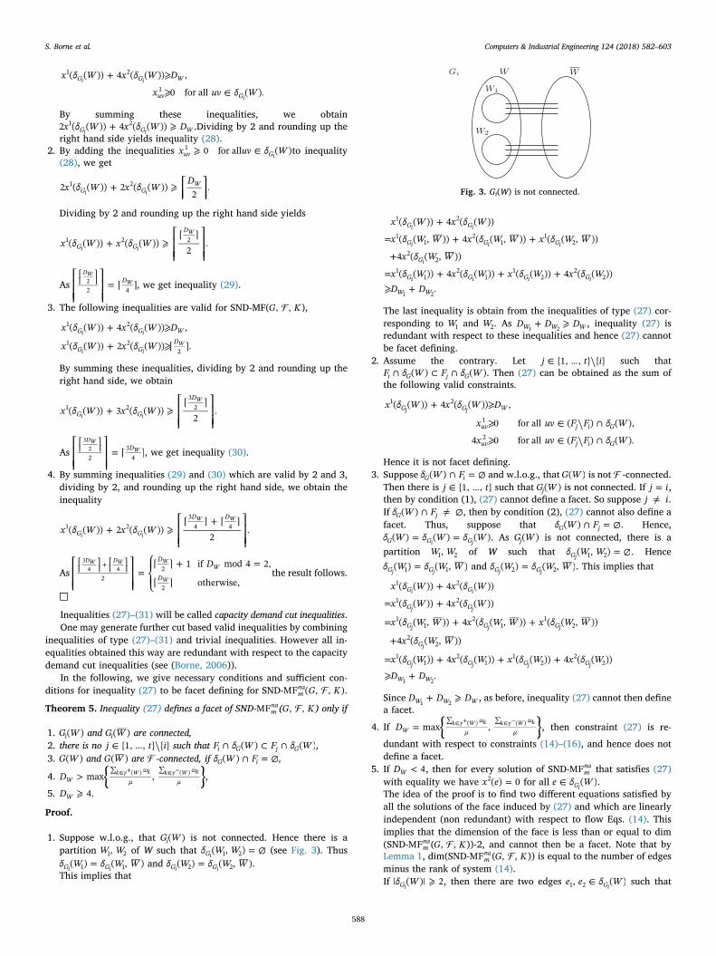
1. Suppose w.l.o.g., that G W( )i is not connected. Hence there is apartition W W,1 2 of W such that = ∅δ W W( , )G 1 2i (see Fig. 3). Thus

=δ W δ W W( ) ( , )G G1 1i iand =δ W δ W W( ) ( , )G G2 2i i

.This implies that

+

= + +

+

= + + +⩾ +

x δ W x δ W

x δ W W x δ W W x δ W W

x δ W W

x δ W x δ W x δ W x δ WD D

( ( )) 4 ( ( ))

( ( , )) 4 ( ( , )) ( ( , ))

4 ( ( , ))

( ( )) 4 ( ( )) ( ( )) 4 ( ( )).

G G

G G G

G

G G G G

W W

1 2

11

21

12

22

11

21

12

22

i i

i i i

i

i i i i

1 2

The last inequality is obtain from the inequalities of type (27) cor-responding to W1 and W2. As + ⩾D D DW W W1 2

, inequality (27) isredundant with respect to these inequalities and hence (27) cannotbe facet defining.

2. Assume the contrary. Let ∈ … ⧹j t i{1, , } { } such that∩ ⊂ ∩F δ W F δ W( ) ( )i G j G . Then (27) can be obtained as the sum of

the following valid constraints.

+ ⩾

⩾ ∈ ⧹ ∩

⩾ ∈ ⧹ ∩

x δ W x δ W D

x uv F F δ W

x uv F F δ W

( ( )) 4 ( ( )) ,

0 for all ( ) ( ),

4 0 for all ( ) ( ).

G G W

uv j i G

uv j i G

1 2

1

2

j j

Hence it is not facet defining.3. Suppose ∩ = ∅δ W F( )G i and w.l.o.g., that G W( ) is not � -connected.

Then there is ∈ …j t{1, , } such that G W( )j is not connected. If =j i,then by condition (1), (27) cannot define a facet. So suppose ≠j i.If ∩ ≠ ∅δ W F( )G j , then by condition (2), (27) cannot also define afacet. Thus, suppose that ∩ = ∅δ W F( )G j . Hence,

= =δ W δ W δ W( ) ( ) ( )G G Gi j . As G W( )j is not connected, there is apartition W W,1 2 of W such that = ∅δ W W( , )G 1 2j

. Hence=δ W δ W W( ) ( , )G G1 1j j

and =δ W δ W W( ) ( , )G G2 2j j. This implies that

+

= +

= + +

+

= + + +

⩾ +

x δ W x δ W

x δ W x δ W

x δ W W x δ W W x δ W W

x δ W W

x δ W x δ W x δ W x δ W

D D

( ( )) 4 ( ( ))

( ( )) 4 ( ( ))

( ( , )) 4 ( ( , )) ( ( , ))

4 ( ( , ))

( ( )) 4 ( ( )) ( ( )) 4 ( ( ))

.

G G

G G

G G G

G

G G G G

W W

1 2

1 2

11

21

12

22

11

21

12

22

i i

j j

j j j

j

j j j j

1 2

Since + ⩾D D DW W W1 2, as before, inequality (27) cannot then define

a facet.

4. If =∑ ∑∈ + ∈ −{ }D max ,W

ω

μ

ω

μk γ W k k γ W k( ) ( ) , then constraint (27) is re-

dundant with respect to constraints (14)–(16), and hence does notdefine a facet.

5. If <D 4W , then for every solution of SND-MFmna that satisfies (27)

with equality we have =x e( ) 02 for all ∈e δ W( )Gi .The idea of the proof is to find two different equations satisfied byall the solutions of the face induced by (27) and which are linearlyindependent (non redundant) with respect to flow Eqs. (14). Thisimplies that the dimension of the face is less than or equal to dim(SND-MFm

na( �G K, , ))-2, and cannot then be a facet. Note that byLemma 1, dim(SND-MFm

na( �G K, , )) is equal to the number of edgesminus the rank of system (14).If ⩾δ W| ( )| 2Gi

, then there are two edges ∈e e δ W, ( )G1 2 isuch that

Fig. 3. Gi(W) is not connected.


588

= =x e x e( ) ( ) 021

22 in every solution satisfying (27) with equality. If,

say, =δ W e( ) { }Gi, then in every solution satisfying (27) with

equality, one should have =x e D( ) W1 and =x e( ) 02 . In both cases,

the two equations are non redundant with respect to (14), and hence(27) cannot define a facet. □

As in Borne et al. (2006), a subgraph =H W F( , ) of =G V E( , ) issaid to be � -connected with respect to � = …F F{ , , }t1 if for all∈ …i t{1, , }, the graph ⧹H Fi is connected.

Theorem 6. Inequality (27) defines a facet of SND-MFmna( �G K, , ) if

1. condition (1), (2), (3), (4) of Theorem 5 are satisfied,2. G W( ) and G W( ) are � -connected.

Proof. See Appendix. □

In Magnanti et al. (1995) introduce cutset inequalities valid for theTwo-Facility Capacitated Network Loading Problem (TFLP). These canbe easily extended to the SND-MFm and the SND-MFs problems. Theextended ones are special cases of the capacity demand cut inequalities.

Corollary 7. Let �∈Fi be an edge subset of ⊆ ∅ ≠ ≠E W V W V, , ,

and let = ⎧⎨⎩

=r

DD4 if mod 4 0,

mod 4 otherwise.WW

WThen the inequality

∑ + ⩾ ⎡⎢⎢

⎤⎥⎥∈

x r x rD

( )4e δ W

e W e WW

( )

1 2

Gi (32)

is valid for both SND-MFm( �G K, , ) and SND-MFs( �G K, , ).

Proof.

• If =r 1W , inequality (32) is nothing but inequality (29).

• If =r 2W , as ⌈ ⌉ = ⌈ ⌉ +2 1D D4 2W W , inequality (32) is nothing but in-

equality (31).

• If =r 3W , as ⌈ ⌉ = ⌈ ⌉3 D D4

34

W W , inequality (32) is nothing but inequality(30).

• If =r 4W , as ⌈ ⌉ = D4 DW4

W , inequality (32) is nothing but inequality(27). □

3.2. Saturation inequalities

In this section we introduce a further class of inequalities which areonly valid for the polytope SND-MFs( �G K, , ). These inequalities arealso induced by cuts in the graph Gi. In these inequalities only the x2

variables, associated with the links with big capacity ( =μ4 10 Gbits),are involved. In fact, the idea behind these inequalities is that if thedemand cannot be routed on the links of a cut with small capacity( =μ 2.5 Gbits), then at least one big capacity must be installed on oneof the links of the cut.

Theorem 8. Let �∈Fi and ⊆ ∅ ≠ ≠W V W V, . Then inequality

⩾⎡

⎢

⎢⎢

∑ ∑ − × ⎤

⎥

⎥⎥

∈ ∈+ −{ }x δ W

ω ω δ W μ

μ( ( ))

max , | ( )|

3Gk γ W k k γ W k G2 ( ) ( )

i

i

(33)

is valid for SND-MFs( �G K, , ).

Proof. By (6) and (27), the following inequalities are valid for SND-MFs( �G K, , )

∑ ∑+ ⩾⎧⎨⎩

⎫⎬⎭∈ ∈+ −

μx δ W μx δ W ω ω( ( )) 4 ( ( )) max , ,G Gk γ W

kk γ W

k1 2

( ) ( )i i

(34)

− − ⩾ − ∈μx e μx e μ e δ W( ) ( ) , for all ( ).G1 2

i (35)

By summing these inequalities, dividing by μ3 and rounding up the

right hand side, we obtain inequality (33). □

In the two following sections we present further classes of validinequalities which are extensions of valid inequalities introduced inBorne et al. (2006) for the problem without capacities.

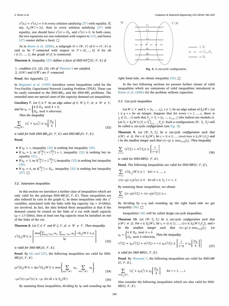
3.3. Cut-cycle inequalities

Let ⊂W V and = … ⩾T e e s{ , , }, 3s1 1 , be an edge subset of δ W( )G . Let⩽ <q s1 be an integer. Suppose that for every = …i s1, , , there is∈ …j t{1, }i such that ∩ = … + −F T e e{ , , }j i i q1 1i

(the indices are modulo s).Let = ⧹ ∪ ⋂= …T δ W T F( ) ( ( ))G i s j2 1 1, , i

. Such a configuration W T T( , , )1 2 willbe called a cut-cycle configuration (see Fig. 4).

Theorem 9. Let W T T( , , )1 2 be a cut-cycle configuration such that≠ ∅γ W( ) . For ∈e δ W( )G , let = ∈ … ∈ ⧹r i s e δ W F|{ {1, , }such that ( ) }|e G ji

andr be the smallest integer such that − ⩾ ∈r s q r( ) max { }e T e2

. Then inequality

∑ + ⩾ ⎡⎢⎢ −

⎤⎥⎥=

x T rx T ss q

( ( ) ( ))l

l l

1,21 2

(36)


Proof. The following inequalities are valid for SND-MF( �G K, , ),

∑ ⩾ = …

− − ⩾ ∈ ==

x δ W i s

r s q r x e e T l

( ( )) 1 for 1, , ,

( ( ) ) ( ) 0 for all , 1, 2.l

lG

el

1,2

2

ji

By summing these inequalities, we obtain

∑ − + − ⩾=

s q x T r s q x T s(( ) ( ) ( ) ( )) .l

l l

1,21 2

By dividing by −s q and rounding up the right hand side we getinequality (36). □

Inequalities (36) will be called design cut-cycle inequalities.

Theorem 10. Let W T T( , , )1 2 be a cut-cycle configuration such that≠ ∅γ W( ) . For ∈e δ W( )G , let = ∈ … ∈ ⧹r i s e δ W F|{ {1, , } | ( ) }|e G ji

, and rbe the smallest integer such that − ⩾ ∈r s q r( ) max { }e T e2

. Let

= ⎧⎨⎩

=r

DD4 if mod 4 0

mod 4 otherwise.WW

WThen the inequality

+ + + × ⩾ ⎡⎢⎢ −

× ⎡⎢⎢

⎤⎥⎥⎤⎥⎥

x T r x T rx T r r x T ss q

rD

( ) ( ) ( ) ( )4W W WW1

12

11

22

2(37)


Proof. By Theorem 7, the following inequalities are valid for SND-MF( �G K, , ),

∑ + ⩾ ⎡⎢⎢

⎤⎥⎥

= …∈

x r x rD

i s( )4

for 1, , .e δ W

e W e WW

( )

1 2

G ji

Also consider the following inequalities which are also valid for SND-MF( �G K, , ).

Fig. 4. A cut-cycle configuration.


589

− − ⩾ ∈− − ⩾ ∈r s q r x e e T

r s q r r x e e T( ( ) ) ( ) 0for all ,

( ( ) ) ( ) 0for all .e

e W

12

22

By summing these inequalities we obtain

∑ ∑− + − + − + − ⩾

× ⎡⎢⎢

⎤⎥⎥

∈ ∈s q x s q r x r s q x r s q r x

s rD

[( ) ( ) ] [ ( ) ( ) ]

4.

e Te W e

e Te W e

WW

1 2 1 2

1 2

By dividing this inequality by −s q and rounding up the right hand sidewe get inequality (37). □

Inequalities (37) will be called capacity cut-cycle inequalities. We canremark that if =r 1W and ⌈ ⌉ = 1D

4W we then obtain the design cut-cycle

inequalities (36).

3.4. Star-partition inequalities

Let =G V E( , ) be a graph and � = …F F{ , , }t1 , with ⩾t 2, a family ofedge subsets of E. Let …V V V, , , p0 1 be a partition of V with p odd.Suppose that for every = …i p1, , , there is ∈ …j t{1, , }i such that

∩ ≠ ∅F V V[ , ]j i 0i. Let = ∈ ∈ ∩ ∩e E e V V F FΛ { | [ , ]k l j jk l

, for some∈ …k l p, {1, , }}. Let = ⋃ ∩ ∪=F F V V( [ , ]) Λi

pj i1 0i

. Such a configurationwill be called a star-partition configuration (see Fig. 5).

Theorem 11. Let …V V V F( , , , , )p0 1 be a star-partition configuration with podd such that ≠ ∅γ W( ) . Then the inequality

∑ … ⧹ ⩾ ⎡⎢⎢

⎤⎥⎥=

x δ V V Fp

( ( , , ) )2l

lG p

1,20

(38)


Proof. It is clear that the following inequalities are valid for SND-MF( �G K, , ).

∑ ⩾ = …

⩾ ∈ ⧹ =

⩾∈ ∩ ⧹

= … = … ≠ =

=⧹x δ V i p

x e e δ V F l

x ee δ V V F F

k p m p k m l

( ( )) 1 for 1, , ,

( ) 0 for all ( ) , 1, 2,

( ) 0for all ( ( , ) ) ,

1, , , 1, , , , 1, 2.

l

lG F i

l

l G k m j j

1,2

0

ji

k m

By summing these inequalities, we obtain inequality

∑ … ⧹ ⩾=

x δ V V F p2 ( ( , , ) ) .l

lp

1,20

By dividing by 2 and rounding up the right hand side, we obtaininequality (38). □

Inequalities (38) will be called design star-partition inequalities.

Theorem 12. Let …V V V F( , , , , )p0 1 be a star-partition configuration.Let

= ⎧⎨⎩

=r

DD4 if mod 4 0,

mod 4 otherwise,VV

Vi

i

i

for = …i p1, , . Set = ∑ = …∈ ⧹

r rei pe δ V

V1, , :

( )G F ji iiand

= ⎧⎨⎩ +

∈ … ⧹λr rr

e δ V V Fif is even,

1 otherwise,( , , )e

e e

eG p0 . Then inequality

∑ ⎜ ⎟⎛⎝

+ ⎞⎠⩾

⎡

⎢

⎢⎢⎢

∑ ⎡⎢

⎤⎥⎤

⎥

⎥⎥⎥∈ … ⧹

=x

λx

r

2 2e δ V V Fe

ee

ip

VD

( , , )

1 2 1 4

G p

iVi

0 (39)


Proof. The following inequalities are valid for SND-MF( �G K, , ).

∑ + ⩾ ⎡⎢⎢

⎤⎥⎥

= …∈ ⧹

x r x rD

i p( )4

for 1, , ,e δ V

e V e VV

( )

1 2

G F ji ii i

i

⩾ ∈ … ⧹

⩾ = … ∈ ⧹

⩾∈ ⧹ ∩

= … = … ≠

⩾∈ ∩ ⧹ = …

= … ≠

⩾∈ ∩ ⧹

= … = … ≠

x e δ V V F

x i p e δ V V F r

xe δ V V F F r

k p m p k m

xe δ V V F F k p

m p k m

xe δ V V F F r

k p m p k m

0 for all ( , , ) ,

0 for 1, , , for all ( , ) , such that is odd,

0for all ( , ) ( ), such that is odd,

1, , , 1, , , ,

0for all ( ( , ) ) , 1, , ,

1, , , ,

0for all ( ( , ) ) , such that is odd,

1, , , 1, , , .

e G p

e G i V

eG k m j j e

eG k m j j

eG k m j j V

10

20

2

1

2

i

k m

k m

k m m

By summing these inequalities we get

∑ + ⩾ ∑ ⎡⎢

⎤⎥∈ … ⧹ =x λ x r(2 )e δ V V F e e e i

sV

D( , , )

1 21 4G p i

Vi0

.

As λe’s, ∈ … ⧹e δ V V F( , , )G p0 are all even, by dividing this inequalityby 2 and rounding up the right hand side we get the inequality

∑ ⎜ ⎟⎛⎝

+ ⎞⎠⩾

⎡

⎢

⎢⎢⎢

∑ ⎡⎢

⎤⎥⎤

⎥

⎥⎥⎥

□∈ … ⧹

=x

λx

r

2 2.

e δ V V Fe

ee

is

VD

( , , )

1 2 1 4

G p

iVi

0

Inequalities (39) are called capacity star-partition inequalities.

3.5. Other valid inequalities

The Arc Residual Capacity inequalities have been introduced inMagnanti et al. (1993) for the Network Loading Problem and used forthe Two-Facility capacitated network loading Problem (Magnanti et al.,1995). In the following we extend these inequalities for our problem.

Theorem 13. Let ⊆L K . Set

∑= = ⎡

⎢⎢⎤⎥⎥

= ⎧⎨⎩

=∈Qω

μσ

Qs

QQ

,4

and4 if mod 4 0,

mod 4 otherwise.Lk L

k

LL

LL

L

Then we have = − +Q σ s4( 1)L L L. Let ∈u v V, 1 and ∈e E2, then theinequality

∑ + − − × ⩽ − −∈μ

f f x s x σ s1 ( ) 2 2 ( 1)(4 )k L

uvk e

vuk e

uv L uv L L, , 1 2

(40)


Proof. Inequality (40) can be written as

∑ + ⩽ − − +∈μ

f f Q s σ x x1 ( ) ( 2 ) 2k L

uvk e

vuk e

L L L uv uv, , 2 1

for ⊆ ∈L K u v V, , 1 and ∈e E2 because − − = −σ s Q σ s( 1)(4 )L L L L L.

• If ⩾x σ2 uv L2 then − − + ⩾Q s σ x x Q( 2 ) 2L L L uv uv L

2 1 .Fig. 5. A star-partition configuration.


590

We know that inequalities (8) are valid for the problem. By sum-ming these inequalities, we obtain

∑ ∑+ ⩽∈ ∈

f f ω( ) .k L

uvk e

vuk e

k Lk

, ,

Then

∑ + ⩽∈μ

f f Q1 ( ) ,k L

uvk e

vuk e

L, ,

which implies that inequality (40) is valid.

• If ⩽ −x σ2 1uv L2 , then

− − + = − + − − +

= − + − − +

Q s σ x x σ s s σ x x

σ s x σ x

( 2 ) 2 4( 1) ( 2 ) 2

4( 1) (2 ( 1)) 2 .L L L uv uv L L L L uv uv

L L uv L uv

2 1 2 1

2 1

Let = −s t4L with ⩽ <t0 4, we obtain.

− − + = − + − − − +

= + + − + −

Q s σ x x σ t x σ x

x x t x σ

( 2 ) 2 4( 1) (4 )(2 ( 1)) 2

8 2 ( 2 ( 1)).L L L uv uv L uv L uv

uv uv uv L

2 1 2 1

2 1 2

Then

− − + ⩾ +Q s σ x x x x( 2 ) 2 8 2 ,L L L uv uv uv uv2 1 2 1 (41)

because ⩾t 0 and ⩽ −x σ2 1uv L2 . As

∑ ∑⩽ + ⩽ +∈ ∈

f μx μx f μx μx4 and 4 ,k K

uvk e

uv uvk K

vuk e

uv uv, 1 2 , 1 2

then ∑ + ⩽ +∈ f f x x( ) 2 8μ k K uvk e

vuk e

uv uv1 , , 1 2 , and hence

∑ + ⩽ +∈μ

f f x x1 ( ) 2 8 .k L

uvk e

vuk e

uv uv, , 1 2

(42)

By (41) and (42), it follows that inequality (40) is valid. □

4. Branch-and-Cut and Branch-and-Cut-and-Price algorithms

In this section, we describe four algorithms for the SND-MF pro-blem. We consider the two variants of the problem (simple and mul-tiple) and for each variant we propose a Branch-and-Cut algorithmbased on the node-arc formulation and a Branch-and-Cut-and-Price al-gorithm based on the path formulation. Our aim is to address the al-gorithmic applications of the previous results.

We now describe the framework of our algorithms. For the Branch-and-Cut algorithms based on the node-arc formulation, we start theoptimization with the linear relaxations of the considered formulations.The optimal solutions x x f( , , )1 2 of theses relaxations are feasible for theSND-MF problems if x1 and x2 are integral.

For the Branch-and-Cut-and-Price algorithms, we start the optimi-zation by solving the linear relaxation of the path formulations. For thiswe use a standard column generation algorithm.

4.1. Column generation

This approach has been extensively used for modeling and solvinglarge scale multicommodity flow problems (Ahuja, Magnanti, & Orlin,1993; Barnhart, Johnson, Nemhauser, Savelsbergh, & Vance, 1998;Lübbecke & Desrosiers, 2004). The general idea of column generation isto solve a restricted linear program (called the master problem) with asmall number of variables (columns) in order to determine an optimalsolution for the master problem. In fact a limited number of variablesmay induce an optimal basic solution for the master problem. So thecolumn generation algorithm solves the linear relaxation of the masterproblem by solving the linear relaxations of several restricted masterproblems. After determining the solution of the linear relaxation of arestricted master problem, we use the pricing problem which consists infinding whether there are any columns not yet in the restricted masterproblem with negative reduced cost. If none can be found, then the

current solution of the restricted master problem is optimal for thelinear relaxation of the master problem. However, if one or more suchcolumns do exist, then they are added to the restricted master problemand the process is repeated until no variable with negative reduced costexists. This approach can be combined with row generation to obtain avery strong method to solve the linear relaxations (see Barnhart, Hane,& Vance, 2000).

To start the column generation scheme, an initial restricted masterproblem has to be provided. This initial problem must have a feasiblesolution to ensure that correct information is passed to the pricingproblem.

For the version of the SND-MF problem with multiple edges (SND-MFm problem), finding an initial feasible solution is very easy. Indeedwe look for shortest paths between the origin-destinations of all com-modities. These paths are then used to carry the flow for each com-modity. As we can install as much capacity as we want, this multi-commodity flow is feasible.

For the SND-MFs problem, we consider an auxiliary master problemwhere =x 0uv

1 and =x 1uv2 for all edge ∈uv E1 (that is to say, we fix the

capacity of each edge to the highest possible value, i.e., = =μ μ4 102Gbits), and the objective is to minimize the maximum excess of flow onany edge (amount of flow exceeding the capacity), denoted ε. If theoptimal solution for this linear program is such that >ε 0, we concludethat the SND-MFs problem has no solution. On the other hand, if =ε 0,then the set of variables used in the column generation permits to havean initial feasible solution for the restricted master problem.

For any restricted master problem, let γ , ϑke

u ve( , ) and ϑ v u

e( , ) be the dual

variables associated with constraints (9)–(11), respectively. The re-duced cost associated with the variable of a path �∈P k

e is= ∑ −∈R γϑP

k eu v P u v

eke,

( , ) ( , ) .The pricing problem can then be reduced to theresolution of several shortest path problems with non-negative costs.Indeed the pricing problem consist in finding for each commodity ∈k Kand each edge ∈e E2, a path P in � k

e such that =RPk e,

�′∈ ′RminP Pk e,

ke and

<R 0Pk e, . Therefore, we can identify columns which have to be added to

the restricted master problem by solving one shortest path problem foreach commodity ∈k K and each edge ∈e E2 in the graph with arc costsequal to ϑ u v

e( , ) for each ∈ ⧹

⎯→⎯u v A F( , ) e

1 . If one or more paths have non-positive reduced cost, then they are added in the restricted masterproblem. Otherwise, the master problem has been solved to optimality.

Combining column and row generation can yield a very stronglinear relaxation. In the next section, we describe some valid inequal-ities. These will be used as cutting planes in our Branch-and-Cut-and-Price algorithm for the two variants of the problem. We introduce someinequalities which are valid for the problem with or without multipleedges.

A solution x x f( , , )1 2 obtained after a column generation phase isfeasible for the SND-MF problems only if x1 and x2 are integral. Usually,such a solution is not feasible, and thus, in each iteration of the Branch-and-Cut and the Branch-and-Cut-and-Price algorithms, it is necessary togenerate further inequalities that are valid for the SND-MF problem butviolated by the current solution x x f( , , )1 2 . For this, one has to solve theso-called separation problem.

4.2. Separation algorithms

Given a class of inequalities, the separation problem associated withthese inequalities consists in deciding whether a solution x x f( , , )1 2

satisfies the inequalities, and if not, in finding an inequality that isviolated by x x f( , , )1 2 . An algorithm which solves this problem is calleda separation algorithm. The inequalities given above are all valid for thefour polytopes SND-MFm

na, SND-MFmp , SND-MFs

na and SND-MFsp except

the saturation inequalities which are valid only for the simple version ofthe problem. Hence these inequalities are used in our algorithms. Theseparation is performed in the following order:

1. arc residual capacity constraints (40) (for the Branch-and-Cut


591

algorithms only),2. design cut constraints (26) and capacity demand cut constraints

(27)–(31),3. saturation constraints (33) (for SND-MFs only),4. design cut-cycle constraints (36),5. capacity cut-cycle constraints (37),6. design star-partition constraints (38),7. capacity star-partition constraints (39).

We remark that all the inequalities are global (i.e., valid in all theBranch-and-Cut tree and the Branch-and-Cut-and-Price tree) and sev-eral constraints may be added at each iteration. Moreover, we go to thenext class of inequalities only if the separation of the previous class ofinequalities does not generate any violated inequality. Our strategy is totry to detect violated constraints at each node of the Branch-and-Cuttree in order to obtain the best possible lower bound and thus limit thenumber of generated nodes. Generated inequalities are added by sets ofat most 200 inequalities at a time.

Now we describe the separation procedures used in our algorithms.All our separation algorithms are applied on =G V E( , )x x x x( , ) ( , )1 2 1 2 wherex x( , )1 2 is the restriction on x1 and x2 of the current LP solution, and

E x x( , )1 2 contains all the edges uv of E such that + ≠x x 0uv uv1 2 .

To separate the design cut inequalities (26) and the capacity de-mand cut inequalities (27)–(31), we have developed a fast heuristic. Wefirst check whether a degree cut ∈δ v v V( ),G x x( 1, 2)

, is violated. Then we

start contracting edges uv with high value+ −∑ ∈ ∪μx μx ω4uv uv k γ u γ v k

1 2({ }) ({ }) until we get a graph on two nodes. In

each iteration we check if the cut associated with the node arising fromthe contraction, induces a violated constraint of type (27), (29), (30) or(31). This runs in O mlogm( ) time where m is the number of edges of G.

When this heuristic does not find any violated inequalities, wecompute the so-called Gomory-Hu tree (Gomory & Hu, 1961) on thegraph G x x( , )1 2 with the weight +x xuv uv

1 2 for each edge uv. This tree hasthe property that for all pairs of nodes ∈s t V, , the minimum (s t, )-cutin the tree is also a minimum (s t, )-cut in G x x( , )1 2 . Actually, we use thealgorithm developed by Gusfield (1990) which requires −V| | 1 max-imum flow computations. The maximum flow computations are han-dled by the efficient Goldberg and Tarjan algorithm (Goldberg &

Tarjan, 1988) that runs inO mn( log )nm

2. Here n is the number of nodes of

G. Then we calculate the right hand side for all the cuts in the Gomory-Hu tree and check if the found constraints are violated.

During the separation of the saturation constraints (33), we considerthe cuts ∈δ v v V( ),G x x( 1, 2)

. We test if these inequalities are violated and

if so we add them to the program. We don’t consider the other cuts ofthe graph G x x( , )1 2 induced by at least two nodes which seem almostnever be violated.

Now we turn our attention to the separation of the cut-cycle in-equalities (36) and (37). For more efficiency, we have used these con-straints only when =q 1. In fact we remarked that the design cut-cycleinequalities and the capacity cut-cycle inequalities which are violatedare usually of this type.

To separate the design cut-cycle constraints with =q 1, we computethe Gomory-Hu tree of the graph G x x( , )1 2 with the weight for each edgeuv equal to the sum +x xuv uv

1 2 . Then for each cut given by the Gomory-Hu tree, with value less than 2, we test if the cut intersects at least onedemand. If this is the case, then it yields a design cut-cycle inequality(36) violated by x x( , )1 2 . Then sets T1 and T2 are determined so that T1 ismaximal, using the following greedy procedure (Algorithm 1). Since theGomory-Hu algorithm runs with a large complexity, in order to accel-erate our separation for the cut-cycle inequalities, we first consider thedegree cuts ∈δ v v V( ),G x x( 1, 2)

. The computation of the Gomory-Hu tree

is considered only if no cuts of this type of value less than 2 are found.

Thus the separation of the cut-cycle inequalities runs in O mn( log )nm

2

time.

Algorithm 1. Algorithm 1

�← ∅ ← ∅ ← ∅T T; ;1 2 ;for =i 1 to m do

if ∈f Fi j0for some ∈ …j t{1, , }0 and ¬ ∈f Fi j for all �∈Fj

then← ∪T T f{ }i1 1 ;

� �← ∪ F{ }j0;

else← ∪T T f{ }i2 2 ;

end ifend forfor all ∈f Ti 2

if ∈f Fi j for all �∈Fj then

← ⧹T T f{ }i2 2 ;end if

end for

For the separation of the capacity cut-cycle constraints, we firstconsider the degree cuts ∈δ v v V( ),G x x( 1, 2)

. We calculate the right hand

side. If the associated constraint is violated, we then determine the setsT1 and T2 using Algorithm 1. Then we start contracting edges until weget a graph on two nodes. In each iteration we contract an edge uv withthe biggest value for + −∑ ∈ ∪μx μx ω4uv uv k γ u γ v k

1 2({ }) ({ }) and check whether

the new node obtained by contraction together with T1 and T2 induces aviolated capacity cut-cycle inequality. This heuristic runs in O m( log m)time.

We now discuss our separation routine for the star-partition in-equalities (38) and (39). We use a linear greedy heuristic which consistsin determining fractional cycles in the supporting graph, satisfyingsome conditions. These cycles have to be odd, in order to have a chanceto find a violated design star-partition inequality. Thus, for each de-tected cycle ( …v v, , p1 ) we try to find edge subsets

∈ … = …F j t i p, {1, , }, 1, ,j iiamong the edges of ⧹ …v V v v[ , { , , }]i p1 in such

a way that either the design star-partition inequality or the capacitystar-partition induced by ⧹ … …V v v v v{ , , }, { }, , { }p p1 1 , and = …F i p, 1, ,ji

is

violated by x x( , )1 2 .To store the generated inequalities, we created a pool whose size

increases dynamically. All the generated inequalities are put in the pooland are dynamic, i.e., they are removed from the current LP when theyare not active. We first separate inequalities from the pool. If all theinequalities in the pool are satisfied by the current LP-solution, then weseparate the classes of inequalities in the order given above.

In the following section, we give some computational results ob-tained with the algorithms presented above for random instances andfor real instances provided by Orange Labs.

5. Computational results

The Branch-and-Cut and Branch-and-Cut-and-Price algorithms de-scribed in the previous section have been implemented in C++, usingABACUS1 (A Branch-And-CUt System) 2.4 alpha (Elf, Gutwenger,Jünger, & Rinaldi, 2001; Thienel et al., 1995) to manage the Branch-and-Cut tree and Cplex 9.02 as LP-solver. It was tested on a Pentium IV2,4 GHz with 1 Gb RAM, running under Linux. We fixed the maximumCPU time to 5 h.

Results are presented here for instances coming from real applica-tions and instances obtained from problems of the TSP Library (Reinelt,1991) by randomly generating the node set, the edge sets Fe and the set

1 http://www.informatik.uni-koeln.de/abacus/.2 www.ibm.com/software/commerce/optimization/cplex-optimizer/.


592

http://www.informatik.uni-koeln.de/abacus/

http://www.ibm.com/software/commerce/optimization/cplex-optimizer/

of demands K. For all the instances, the graph G1, representing the IPnetwork, is considered complete.

These instances were generated with 6, 8 and 10 nodes, � =| | 10, 20and =K| | 5, 10, 20. Five instances of each size, each �| | and each K| |were tested. We will consider the average results obtained for theseinstances.

The real instances are extracted from operational networks and havebeen provided by the french telecommunications operator FranceTélécom. These instances have 6 to 18 nodes and � with 11 to 32 edgesets. Actually France Télécom has provided the optical network and therouting between every pair of nodes in this network. With an edge f ofthe IP network, we associate the routing path of the optical networkbetween the switches corresponding to the IP router endpoints of f.Using these paths, we have computed � = ⊆ ∈F E e E{ , }e

1 2 where Fe isthe set of edges f of E1 such that e belongs to the path associated with f.

The number of commodities is between 5 and 20. We randomlygenerated the endpoints of the commodities. The amount of eachcommodity is calculated with the gravity model. This model, in-troduced by Reilly (1931) and inspired from Newton’s law of gravita-tion, permits to predict the movement of people and commodities be-tween cities and continents. The model uses the distance and thepopulation of both, the origin and destination cities. The general ex-pression of the gravity model for a commodity o d v( , , )k k k of K is

=vkP P

dokα

dkβ

ok dk,where Pok

and Pdkare the populations of the origin and des-

tination cities, respectively, and do d,k krepresents the euclidean distance

between ok and dk. The amount of traffic we consider is rvk where r is aconstant. We fix =r 1.2 and =r 0.8 in order to have different amounts

of traffic between two cities in the two directions, and then break thesymmetry.

Usually the cost associated with a link in the client network is re-lated to the corresponding routing path in the optical network, and thendepends on the cost of this path. Actually, the cost c f( ) of link f in the IPnetwork is given by

= +c f c κ f( ) ( ),

where c is a fixed cost representing the equipments of the extremityports on the routers of f in the IP layer, and κ f( ) is a cost depending onthe length of the path Pf corresponding to f in the optical network.

The installation of an optical link usually yields a fixed cost on eachextremity of this link. Hence a first estimation of the optical cost κ f( ) isthe sum of the fixed costs of the optical links on Pf . As these fixed costscan be considered the same in the optical network, a good approachwould be to consider a cost κ f( ) proportional to the number of theoptical links on Pf . So, a first natural function κ f( ) consists of thenumber of links (hops) in the optical path between the switching nodescorresponding to the endpoints of f. Here we assume that there is a fixedcost associated with each optical link. This cost is considered once thecorresponding link is used. Then the cost c f( ) is given in this case by+c P| |f .In the various tables, the entries are:

V| |1 : the number of nodes of G1,�| | : the number of sets Fe,K| | : the number of demands,FV :

Table 1Results for random instances for the SND-MFm problem.

�V K(| |, | |, | |)1 FV NC NRC NCC NSP NT o/p Gap TT

Algorithm based on the node-arcs formulation(6,10,5) 1500 85.67 78.00 0.67 0.67 132.33 3/3 9.47 0:00:14(6,10,10) 3000 80.00 89.00 0.00 0.00 109.67 3/3 5.86 0:00:40(6,10,20) 6000 71.33 201.00 0.33 0.00 123.00 3/3 6.39 0:02:23(6,20,5) 3000 105.00 226.33 2.00 0.67 220.33 3/3 10.74 0:01:38(6,20,10) 6000 125.67 427.67 2.67 0.00 214.33 3/3 8.41 0:04:28(6,20,20) 12,000 153.33 641.00 0.33 0.00 347.00 3/3 7.46 0:33:30(8,10,5) 2800 104.00 84.00 0.67 0.33 115.00 3/3 12.09 0:00:38(8,10,10) 5600 304.33 449.67 2.00 1.00 771.00 3/3 10.68 0:16:58(8,10,20) 11,200 381.33 1290.00 0.00 0.00 2585.00 1/3 9.60 4:13:52(8,20,5) 5600 282.67 1102.33 2.00 0.67 1041.00 3/3 14.84 0:30:23(8,20,10) 11,200 281.00 1524.67 2.00 0.67 2454.00 0/3 25.13 5:00:00(8,20,20) 22,400 283.00 3726.00 1.00 0.00 1266.33 0/3 15.30 5:00:00(10,10,5) 4500 819.67 519.33 0.33 0.33 2282.33 3/3 13.58 0:34:05(10,10,10) 9000 846.33 1188.67 1.00 0.00 1773.67 3/3 9.81 1:39:04(10,10,20) 18,000 524.67 1325.33 0.33 0.67 1144.00 2/3 33.42 3:22:06(10,20,5) 9000 199.33 2140.00 0.67 0.00 2653.00 1/3 38.60 4:05:10(10,20,10) 18,000 378.33 5020.00 0.67 0.00 1523.67 0/3 33.59 5:00:00(10,20,20) 36,000 491.00 4169.33 0.67 0.00 457.00 0/3 45.39 5:00:00

Algorithm based on the path formulation(6,10,5) 590.67 93.33 – 0.33 0.67 112.33 3/3 9.40 0:00:07(6,10,10) 899.33 92.67 – 0.00 0.00 95.00 3/3 5.24 0:00:08(6,10,20) 1363.33 124.67 – 0.00 0.00 157.00 3/3 5.96 0:00:15(6,20,5) 813.33 118.33 – 1.67 0.00 237.67 3/3 10.71 0:00:34(6,20,10) 1490.00 156.67 – 1.00 0.00 165.67 3/3 8.29 0:00:39(6,20,20) 2326.00 156.33 – 0.33 0.00 297.00 3/3 7.38 0:01:46(8,10,5) 1094.00 91.67 – 0.33 0.33 121.67 3/3 11.35 0:00:23(8,10,10) 2769.33 457.00 – 0.67 0.00 876.33 3/3 10.31 0:04:58(8,10,20) 4100.00 2083.00 – 1.33 0.00 3334.33 3/3 9.48 0:23:00(8,20,5) 3324.67 246.33 – 2.67 1.00 1223.67 3/3 11.89 0:21:40(8,20,10) 5937.33 5472.00 – 1.67 2.00 9515.67 2/3 13.63 3:12:00(8,20,20) 5619.00 1733.33 – 0.67 0.00 5004.67 2/3 10.64 1:57:35(10,10,5) 7192.67 1271.33 – 0.33 0.00 2159.00 3/3 11.49 0:52:43(10,10,10) 8197.33 2775.00 – 0.67 0.00 3378.33 3/3 9.98 1:45:52(10,10,20) 12500.00 2773.67 – 1.00 0.00 11246.67 0/3 12.38 5:00:00(10,20,5) 6991.00 1249.33 – 3.67 5.00 3978.33 1/3 33.94 3:59:40(10,20,10) 11784.00 5659.67 – 2.67 2.33 3953.00 1/3 26.08 4:33:09(10,20,20) 14427.33 3986.67 – 1.00 0.67 3665.00 0/3 33.98 5:00:00


593

the number of flow variables for the node-arc formulationand thenumber of generated paths for the path formulation,

NC : the number of generated cut inequalities,NRC : the number of generated arc residual capacity inequalities,NS : the number of generated saturation inequalities (only for

SND-MFs problem),NCC : the number of generated cut-cycle inequalities,NSP : the number of generated star-partition inequalities,NT : the number of generated nodes in the Branch-and-Cut tree,o/p : the number of problems solved to optimality over the

numberof instances tested (only for random instances),

Copt : the value of the optimal solution,Gap : the relative error between the best upper bound (the optimal

value if the problem has been solved to optimality) and thelower bound achieved by the cutting plane phase (beforebranching),

TT : the total CPU time in h:mm:ss.Our first series of experiments concerns the problem SND-MFm (with

multiple links) for the random instances. In these experiments, we haveconsidered three instances for each size. Table 1 reports the averageresults obtained for these instances with both algorithms based on the

node-arc and the path formulations.As we can observe, all the instances with 6 nodes have been solved

to optimality. Moreover, they have been solved in less than 5min (andin less than 2min using the path formulation based algorithm), exceptthose with � =| | 20 and =K| | 20. These needed around 33min to besolved to optimality using the node-arc formulation based algorithm.We also remark that for the instances with a reduced number of com-modities, the problem seems to be much easier to solve. In fact, for allthe instances with 5 commodities, less than one hour was needed to getthe optimal solution except for the instances with 10 nodes and� =| | 20.

The instances with 10 and 20 commodities and � =| | 20 seem to beharder to solve. In fact, none of these instances could be solved to op-timality with the node-arc formulation within the time limit, when thenumber of nodes exceeds 8. The results are more promising with thepath formulation where 5 instances among 12 have nevertheless beensolved in an average time sometimes less than two hours.

Among the 54 tested instances, 17 could not be solved within thetime limit of five hours using the node-arc formulation based algorithm,and only 12 instances with that based on the path formulation. So, thiswould imply that the latter algorithm is more efficient. However for 10nodes, � =| | 10 and =K| | 20, two instances have been solved with thefirst algorithm but they did not with the second one.

Table 2Results for real instances for the SND-MFm problem.

�V K(| |, | |, | |)1 FV NC NRC NCC NSP NT Copt Gap TT

Algorithm based on the node-arcs formulation(6,11,5) 1650 10 10 0 1 3 57 0.00 0:00:01(6,11,10) 3300 56 111 2 3 65 99 8.08 0:00:27(6,11,15) 4950 99 779 1 0 157 105 7.62 0:02:42(6,11,20) 6600 199 1194 1 0 375 115 9.57 0:13:34(8,17,5) 4760 173 114 2 0 115 81 11.11 0:02:37(8,17,10) 9520 191 717 2 7 567 109 15.60 0:50:00(8,17,15) 14,280 512 815 4 2 621 123 13.01 2:12:27(8,17,20) 19,040 666 9743 7 5 709 160 33.75 5:00:00(10,25,5) 11,250 71 157 4 0 113 129 7.75 0:16:28(10,25,10) 23,400 262 279 4 2 369 156 3.21 2:45:11(10,25,15) 33,750 772 1616 6 0 473 231 18.18 5:00:00(10,25,20) 45,000 447 2754 6 1 247 297 34.34 5:00:00(12,32,5) 21,120 85 180 5 0 99 129 8.53 0:54:34(12,32,10) 42,240 333 777 5 1 303 194 12.37 5:00:00(12,32,15) 63,360 251 1129 8 0 127 300 32.67 5:00:00(12,32,20) 84,480 357 2001 7 0 89 392 41.58 5:00:00(14,27,5) 24,570 55 22 0 0 73 150 8.00 0:34:17(14,27,10) 49,140 342 298 2 0 175 198 6.06 4:56:12(16,29,5) 34,800 315 208 3 0 323 153 11.76 5:00:00(16,29,10) 69,600 88 206 1 0 67 185 4.32 4:21:11(18,30,5) 45,900 87 234 2 0 229 218 17.43 5:00:00

Algorithm based on the path formulation(6,11,5) 137 15 – 0 0 3 57 0.00 0:00:01(6,11,10) 628 59 – 2 1 81 99 8.08 0:00:07(6,11,15) 1071 88 – 1 0 147 105 7.62 0:00:18(6,11,20) 1778 233 – 1 0 451 115 9.57 0:01:38(8,17,5) 1693 178 – 1 0 93 81 11.11 0:00:55(8,17,10) 3452 180 – 2 5 449 109 15.60 0:07:13(8,17,15) 4717 511 – 4 2 1155 123 14.63 0:18:48(8,17,20) 8230 2570 – 5 19 5655 131 19.08 3:34:26(10,25,5) 4011 99 – 2 0 151 129 8.53 0:08:16(10,25,10) 5594 318 – 2 4 373 156 3.21 0:43:36(10,25,15) 8673 5497 – 5 0 3993 213 11.27 5:00:00(10,25,20) 8966 4038 – 9 3 3317 261 24.90 5:00:00(12,32,5) 7188 100 – 2 0 153 129 8.53 0:34:49(12,32,10) 15,120 572 – 4 1 559 182 6.59 5:00:00(12,32,15) 8852 262 – 5 2 127 285 28.77 5:00:00(12,32,20) 13,988 1109 – 7 0 681 378 39.15 5:00:00(14,27,5) 4081 44 – 0 0 49 150 8.00 0:10:56(14,27,10) 17,610 608 – 1 0 205 198 6.06 5:00:00(16,29,5) 15,910 294 – 3 0 177 159 15.09 5:00:00(16,29,10) 19,934 114 – 2 0 77 185 4.32 3:26:08(18,30,5) 21,494 47 – 0 0 63 220 18.64 5:00:00


594

The number of flow variables of the node-arc formulation is fixedand only depends on �V| |, | |1 and K| |. This is not however the case forthe flow variables of the path formulation. We remark that the numberof the flow variables generated, using this formulation, is generallysmaller than that of the node-arc formulation. For example if we con-sider the instance with 8 nodes, 20 commodities and � =| | 10, we havethat the number of flow variables is 11200 whereas the number ofgenerated paths is 4100. This may explain the fact that some instancescould be solved to optimality using the path formulation whereas theycould not using the node-arc one. Moreover the CPU times obtainedwith the path formulation based algorithm are less than those obtainedwith the node-arc formulation based algorithm except for the instanceswith 10 nodes and � =| | 10. The difference of time is sometimes big. Forexample, for the instances with 6 nodes, � =| | 20 and =K| | 20, the timegoes from less than 2min to more than 30min and for 8 nodes, � =| | 10and =K| | 20, it goes from 20min to more than 4 h. Therefore the pathformulation seems to give better results than the node-arc formulation.

We can also remark that for most of the instances, a significantnumber of cut and arc residual capacity inequalities (for the node-arcformulation) have been generated. This implies that these inequalitiesare useful for the random problems. However the cut-cycle and star-partition inequalities do not seem to play an important role for this typeof instances.

Table 2 presents the results for the SND-MFm problem for the realinstances with both path and node-arc formulation based algorithms.Here the cost function represents, for each link of the IP network, thenumber of links of the optical network used in the associated path. Thiscost function is then integral.

It appears from the table that the difficulty to solve the instancesincreases with the number of nodes and the number of commodities inthe network. All the instances with 5 commodities and up to 14 nodeshave been solved in less than one hour. Also for the instances with 10commodities, we have obtained an optimal solution for all the instanceswith no more than 10 nodes in less than 3 h with the node-arc for-mulation and in less than 45min with the path formulation. The in-stance with 16 nodes and 10 commodities has also been solved to op-timality.

In addition, we remark that for the instances with 15 and 20 com-modities only those with no more than 8 nodes could be solved tooptimality. For all the instances which have not been solved in the timelimit, we have nevertheless obtained feasible solutions (given in italic).Also, we can remark that for some instances, we have obtained a re-latively small gap. This is for example the case for the instance with 12nodes and 10 commodities where the gap is 6%. For the larger in-stances, the gap does not exceed 18%.

Moreover we notice that all the instances solved with the algorithmbased on the node-arc formulation have also been solved with the onebased on the path formulation, except that with 14 nodes and 10commodities. Furthermore, the time needed was much lower. In fact, asit can be observed, for the instance with 8 nodes and 15 commodities,the time passes from 2 h 12min to 18min and for that with 10 nodesand 10 commodities, it passes from 2 h 45min to 43min. As regards theinstances which have not been solved with the two algorithms in thetime limit, we can remark that the value of the best feasible solution wehave found with the path formulation is cheaper than that obtainedwith the node-arc one and this is for most of the instances.

Table 3Results for random instances for the SND-MFs problem.

�V K| |, | |, | |1 FV NC NRC NS NCC NSP NT o/p Gap TT

Algorithm based on the node-arcs formulation(6,10,5) 1500 58.67 49.67 3.67 0.33 0.00 46.33 3/3 14.04 0:00:08(6,10,10) 3000 43.67 47.33 4.67 0.00 0.00 23.67 3/3 4.48 0:00:15(6,10,20) 6000 48.67 96.67 3.33 0.00 0.00 36.33 3/3 6.63 0:01:17(6,20,5) 3000 75.67 151.00 3.00 1.67 0.33 106.33 3/3 16.16 0:01:05(6,20,10) 6000 70.67 187.33 9.67 1.00 0.00 41.00 3/3 9.93 0:01:29(6,20,20) 12,000 44.67 94.33 2.67 0.00 0.00 24.33 3/3 6.22 0:03:12(8,10,5) 2800 81.67 97.33 0.67 0.33 0.33 85.00 3/3 13.16 0:00:46(8,10,10) 5600 215.33 293.00 2.33 0.67 0.00 296.33 3/3 10.02 0:06:35(8,10,20) 11,200 277.00 773.33 4.33 0.00 0.00 373.67 3/3 9.02 0:30:53(8,20,5) 5600 177.33 570.33 1.00 1.67 0.67 118.33 3/3 13.43 0:05:30(8,20,10) 11,200 381.00 1140.00 11.00 0.67 0.67 772.33 3/3 14.34 1:38:42(8,20,20) 22,400 305.67 1988.00 13.00 0.33 0.00 639.67 1/3 12.44 3:50:49(10,10,5) 4500 189.67 510.00 0.00 0.00 0.00 412.00 3/3 18.06 0:06:53(10,10,10) 9000 171.33 610.00 2.00 0.00 0.00 1379.00 3/3 11.49 1:39:01(10,10,20) 18,000 176.67 823.33 0.00 1.00 0.33 1214.00 2/3 15.42 2:54:21(10,20,5) 9000 314.00 1293.00 0.00 3.00 0.00 507.00 1/3 22.14 3:29:34(10,20,10) 18,000 740.00 5198.00 0.00 1.00 0.00 1463.00 0/3 34.28 5:00:00(10,20,20) 36,000 448.67 4156.33 1.67 0.67 0.00 464.33 0/3 27.72 5:00:00

Algorithm based on the path formulation(6,10,5) 550.67 85.00 – 3.33 0.33 0.33 52.33 3/3 13.93 0:00:05(6,10,10) 776.67 39.57 – 4.67 0.33 0.00 29.67 3/3 4.54 0:00:03(6,10,20) 836.67 21.00 – 1.33 0.00 0.00 17.00 3/3 4.93 0:00:02(6,20,5) 812.00 55.67 – 3.00 2.00 0.00 93.67 3/3 15.82 0:00:16(6,20,10) 1194.33 49.33 – 8.67 2.00 0.00 50.33 3/3 9.02 0:00:11(6,20,20) 1532.33 44.33 – 3.67 0.00 0.00 24.33 3/3 7.58 0:00:08(8,10,5) 1225.33 90.67 – 1.00 1.00 0.67 81.67 3/3 12.42 0:00:20(8,10,10) 1910.67 259.00 – 2.33 2.33 0.00 270.33 3/3 9.16 0:01:15(8,10,20) 2912.00 328.67 – 4.33 0.00 0.00 309.67 3/3 8.76 0:02:02(8,20,5) 2514.67 164.67 – 1.33 3.00 0.33 135.67 3/3 12.71 0:02:31(8,20,10) 4944.00 623.67 – 10.00 1.00 0.33 1890.33 3/3 14.12 0:53:32(8,20,20) 5373.00 425.00 – 17.33 0.33 0.00 1000.33 3/3 10.79 0:32:18(10,10,5) 7362.00 1036.33 – 0.00 0.33 0.00 2625.00 2/3 15.75 1:47:00(10,10,10) 8874.00 873.00 – 0.33 2.00 0.00 2756.33 3/3 12.60 2:02:10(10,10,20) 12624.00 1534.33 – 0.67 1.33 0.00 7562.67 1/3 11.87 2:41:08(10,20,5) 10438.67 722.67 – 1.33 6.67 1.33 2799.67 1/3 22.90 3:29:29(10,20,10) 13042.00 2816.67 – 0.00 4.33 2.00 3395.67 0/3 15.92 5:00:00(10,20,20) 14828.00 3292.33 – 3.33 1.33 0.00 3321.00 0/3 17.82 5:00:00


595

As for the random problems, for most of the real instances, a sig-nificant number of cut inequalities have been generated. It also appearsthat the cut-cycle inequalities and star-partition inequalities are moreeffective for this type of instances. This can be explained by the fact thatthe way the sets Fe’s are built, it is easier to find cut-cycle and star-partition configurations. It seems that the node-arc formulation permitsto generate more cut-cycle inequalities (72 constraints generated for allthe instances against 58 with the path formulation) and the path for-mulation privileges rather the star-partition inequalities (37 constraintsgenerated against only 22 with the node-arc formulation).

For these instances, we can also observe that the number of flowvariables generated for the path formulation is much lower than the oneused in the node-arc one. For example, the instance with 16 nodes and10 commodities has used 69600 flow variables for the first formulationand only 19934 flow variables in the second one.

Tables 3 and 4 report the results for the SND-MFs problem (singleversion). As in the previous experiments related to the SND-MFm pro-blem, we have considered random and real instances. We have testedour two algorithms on the same instances. Table 3 reports the results forthe random instances. As for the multiple case, we have tested threeinstances for each size, Table 3 gives the average results. Also here wehave used the saturation constraints (33) which are valid for this var-iant of the problem.

We can note that all the instances with 6 and 8 nodes have beensolved to optimality with at least one of the algorithms. This is also thecase for all the instances with � =| | 10 except that with 10 nodes and 20commodities, and for the instances with =K| | 5, except two of the in-stances with 10 nodes and � =| | 20.

Among the 9 instances with 10 nodes and � =| | 20, only one hasbeen solved in the time limit of 5 h. The gap obtained is generally notvery high (less than 18%). Also here both algorithms seem to have si-milar performance. In fact most of the instances solved by one have alsobeen solved by the other.

The saturation constraints appear in a small proportion with respectto the cut and arc residual capacity inequalities. This does not implythat these inequalities are not necessary for this variant of the problem.On the contrary, they have been quite utile for solving the randominstances. Also we notice that for the multiple variant of the problem,the number of generated cut-cycle and star-partition inequalities is alsonot very significant in this case.

Table 4 presents the results obtained for the SND-MFs problem forthe real instances. We can remark that in general, the results based onthe path formulation, obtained with the Branch-and-Cut-and-Price al-gorithm, are better than those based on the node-arc formulation. Infact, several instances which have not been solved in the time limit withthe latter formulation, have been solved with the former one, and even

Table 4Results for real instances for the SND-MFs problem.

�V K(| |, | |, | |)1 FV NC NRC NS NCC NSP NT Copt Gap TT

Algorithm based on the node-arcs formulation(6,11,5) 1650 12 21 0 0 1 3 57 0.00 0:00:06(6,11,10) 3300 46 137 1 2 0 79 104 10.58 0:00:58(6,11,15) 4950 71 389 1 1 0 75 109 11.01 0:01:39(6,11,20) 6600 72 705 1 1 0 191 122 9.84 0:09:39(8,17,5) 4760 187 101 1 1 0 97 82 12.20 0:01:46(8,17,10) 9520 165 955 4 5 4 777 115 20.00 1:23:37(8,17,15) 14,280 320 3983 3 8 0 981 129 22.48 4:00:52(8,17,20) 19,040 550 8849 3 10 3 771 143 25.87 5:00:00(10,25,5) 11,250 44 135 2 4 0 31 129 8.53 0:04:04(10,25,10) 23,400 82 47 1 0 0 17 157 3.82 0:05:30(10,25,15) 33,750 553 1743 2 4 0 485 223 13.90 5:00:00(10,25,20) 4500 336 3346 2 6 0 227 261 24.52 5:00:00(12,32,5) 21,120 49 215 1 4 0 37 129 7.75 0:21:12(12,32,10) 42,240 233 485 1 4 0 291 186 8.60 5:00:00(12,32,15) 63,360 211 1125 1 4 0 139 247 18.22 5:00:00(12,32,20) 84,480 224 1087 1 7 0 79 317 27.44 5:00:00(14,27,5) 24,570 57 33 0 0 0 41 150 4.67 0:19:09(14,27,10) 49,140 512 387 0 0 0 231 226 17.26 5:00:00(16,29,5) 34,800 343 316 0 1 0 265 158 13.92 5:00:00(16,29,10) 69,600 85 171 0 1 0 45 191 5.76 2:16:09(18,30,5) 45,900 68 262 1 3 0 229 211 14.69 5:00:00

Algorithm based on the path formulation(6,11,5) 103 4 – 2 4 0 1 57 0.00 0:00:01(6,11,10) 618 31 – 1 3 0 89 104 10.58 0:00:06(6,11,15) 931 48 – 1 2 0 57 109 10.09 0:00:07(6,11,20) 1496 47 – 1 3 0 173 122 9.84 0:00:28(8,17,5) 1549 109 – 1 2 0 61 82 12.20 0:00:28(8,17,10) 2950 118 – 2 6 6 1069 115 20.00 0:12:14(8,17,15) 4267 226 – 3 12 1 777 129 19.38 0:17:21(8,17,20) 5856 391 – 3 12 7 731 135 20.74 0:25:56(10,25,5) 3043 37 – 2 5 0 73 129 6.98 0:02:59(10,25,10) 1316 69 – 1 1 0 15 157 3.82 0:00:09(10,25,15) 8220 1484 – 2 8 0 2015 207 7.25 2:42:47(10,25,20) 10,380 1105 – 2 8 0 1457 243 18.93 5:00:00(12,32,5) 6497 84 – 1 4 0 97 129 8.53 0:17:26(12,32,10) 13,723 421 – 1 4 0 851 182 6.59 5:00:00(12,32,15) 15,291 512 – 1 10 6 813 224 9.82 5:00:00(12,32,20) 12,114 615 – 1 12 0 823 292 20.55 5:00:00(14,27,5) 4326 53 – 0 0 0 27 150 5.33 0:07:45(14,27,10) 18,212 652 – 1 4 0 281 208 10.10 5:00:00(16,29,5) 18,949 338 – 0 3 0 119 158 13.92 5:00:00(16,29,10) 13,563 80 – 0 3 0 23 191 5.76 0:17:14(18,30,5) 23,332 43 – 1 3 0 77 231 22.08 5:00:00


596

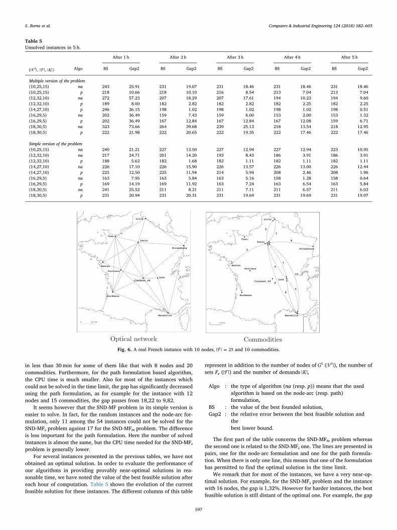
in less than 30min for some of them like that with 8 nodes and 20commodities. Furthermore, for the path formulation based algorithm,the CPU time is much smaller. Also for most of the instances whichcould not be solved in the time limit, the gap has significantly decreasedusing the path formulation, as for example for the instance with 12nodes and 15 commodities, the gap passes from 18,22 to 9,82.

It seems however that the SND-MF problem in its simple version iseasier to solve. In fact, for the random instances and the node-arc for-mulation, only 11 among the 54 instances could not be solved for theSND-MFs problem against 17 for the SND-MFm problem. The differenceis less important for the path formulation. Here the number of solvedinstances is almost the same, but the CPU time needed for the SND-MFsproblem is generally lower.

For several instances presented in the previous tables, we have notobtained an optimal solution. In order to evaluate the performance ofour algorithms in providing provably near-optimal solutions in rea-sonable time, we have noted the value of the best feasible solution aftereach hour of computation. Table 5 shows the evolution of the currentfeasible solution for these instances. The different columns of this table

represent in addition to the number of nodes of G1 (V| |1 ), the number ofsets Fe (�| |) and the number of demands K| |,

Algo : the type of algorithm (na (resp. p)) means that the usedalgorithm is based on the node-arc (resp. path)formulation,

BS : the value of the best founded solution,Gap2 : the relative error between the best feasible solution and

thebest lower bound.

The first part of the table concerns the SND-MFm problem whereasthe second one is related to the SND-MFs one. The lines are presented inpairs, one for the node-arc formulation and one for the path formula-tion. When there is only one line, this means that one of the formulationhas permitted to find the optimal solution in the time limit.

We remark that for most of the instances, we have a very near-op-timal solution. For example, for the SND-MFs problem and the instancewith 16 nodes, the gap is 1,32%. However for harder instances, the bestfeasible solution is still distant of the optimal one. For example, the gap

Table 5Unsolved instances in 5 h.

After 1 h After 2 h After 3 h After 4 h After 5 h

�V K(| |, | |, | |)1 Algo BS Gap2 BS Gap2 BS Gap2 BS Gap2 BS Gap2

Multiple version of the problem(10,25,15) na 243 25.91 231 19.07 231 18.46 231 18.46 231 18.46(10,25,15) p 218 10.66 218 10.10 216 8.54 213 7.04 213 7.04(12,32,10) na 272 57.23 207 18.29 207 17.61 194 10.23 194 9.60(12,32,10) p 189 8.00 182 2.82 182 2.82 182 2.25 182 2.25(14,27,10) p 246 26.15 198 1.02 198 1.02 198 1.02 198 0.51(16,29,5) na 202 36.49 159 7.43 159 6.00 153 2.00 153 1.32(16,29,5) p 202 36.49 167 12.84 167 12.84 167 12.08 159 6.71(18,30,5) na 323 73.66 264 39.68 239 25.13 218 13.54 218 12.95(18,30,5) p 222 21.98 222 20.65 222 19.35 222 17.46 222 17.46

Simple version of the problem(10,25,15) na 240 21.21 227 13.50 227 12.94 227 12.94 223 10.95(12,32,10) na 217 24.71 201 14.20 193 8.43 186 3.91 186 3.91(12,32,10) p 188 5.62 182 1.68 182 1.11 182 1.11 182 1.11(14,27,10) na 226 17.10 226 15.90 226 13.57 226 13.00 226 12.44(14,27,10) p 225 12.50 225 11.94 214 5.94 208 2.46 208 1.96(16,29,5) na 163 7.95 163 5.84 163 5.16 158 1.28 158 0.64(16,29,5) p 169 14.19 169 11.92 163 7.24 163 6.54 163 5.84(18,30,5) na 241 25.52 211 8.21 211 7.11 211 6.57 211 6.03(18,30,5) p 231 20.94 231 20.31 231 19.69 231 19.69 231 19.07

Fig. 6. A real French instance with 10 nodes, � =| | 25 and 10 commodities.


597

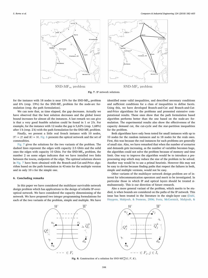
for the instance with 18 nodes is near 15% for the SND-MFm problemand 6% (resp. 19%) for the SND-MFs problem for the node-arc for-mulation (resp. the path formulation).

We can note that, as time elapsed, the gap decreases. Actually wehave observed that the best solution decreases and the global lowerbound increases for almost all the instances. A last remark we can giveis that a very good feasible solution could be found in 1 or 2 h. Forexample, for the instance with 12 nodes the gap is 5,62% (resp. 1,68%)after 1 h (resp. 2 h) with the path formulation for the SND-MFs problem.

Finally, we present a little real french instance with 10 nodes,� =| | 25 and =K| | 10. Fig. 6 presents the optical network and the set ofcommodities.

Fig. 7 gives the solutions for the two variants of the problem. Thedashed lines represent the edges with capacity 2.5 Gbits and the solidones the edges with capacity 10 Gbits. For the SND-MFm problem, thenumber 2 on some edges indicates that we have installed two linksbetween the towns, endpoints of the edge. The optimal solutions shownin Fig. 7 have been obtained with the Branch-and-Cut-and-Price algo-rithm based on the path formulation in 43min for the multiple versionand in only 10 s for the simple one.

6. Concluding remarks

In this paper we have considered the multilayer survivable networkdesign problem which has applications to the design of reliable IP-over-optical network. We have considered the capacity dimensioning of thenetwork. We have proposed two integer programming formulations foreach of the two variants of the problem, simple and multiple. We have

identified some valid inequalities, and described necessary conditionsand sufficient conditions for a class of inequalities to define facets.Using this, we have developed Branch-and-Cut and Branch-and-Cut-and-Price algorithms for the problems and presented extensive com-putational results. These ones show that the path formulation basedalgorithm performs better than the one based on the node-arc for-mulation. The experimental results also show the effectiveness of thecapacity demand cut, the cut-cycle and the star-partition inequalitiesfor the problem.

Both algorithms have only been tested for small instances with up to10 nodes for the random instances and to 18 nodes for the reals ones.First, this was because the real instances for such problems are generallyof small size. Also, we have remarked that when the number of scenariosand demands gets increasing, as the number of variables becomes huge,the algorithm could not solve the problem because of memory and timelimit. One way to improve the algorithm would be to introduce a pre-processing step which may reduce the size of the problem to be solved.Another way would be to use a primal heuristic. However this may notbe easy to devise because finding paths that respect the failures in both,simple and multiple versions, would not be easy.

Other variants of the multilayer network design problem are of in-terest for telecommunication operators and merit to be investigated. Inparticular those in which IP and optical layers should be treated si-multaneously. This is our direction of future research.

Also a more general variant of the problem, which merits to be stu-died, is when bounds are considered on the paths of the IP network. Thisissue has been treated in the literature in the single-layer case (Dahl,Huygens, Mahjoub, & Pesneau, 2006; Fortz, McCormick, Mahjoub, &

Fig. 7. IP network solutions.

Fig. 8. Construction of a solution for �G KSND-MF ( , , )mna .


598

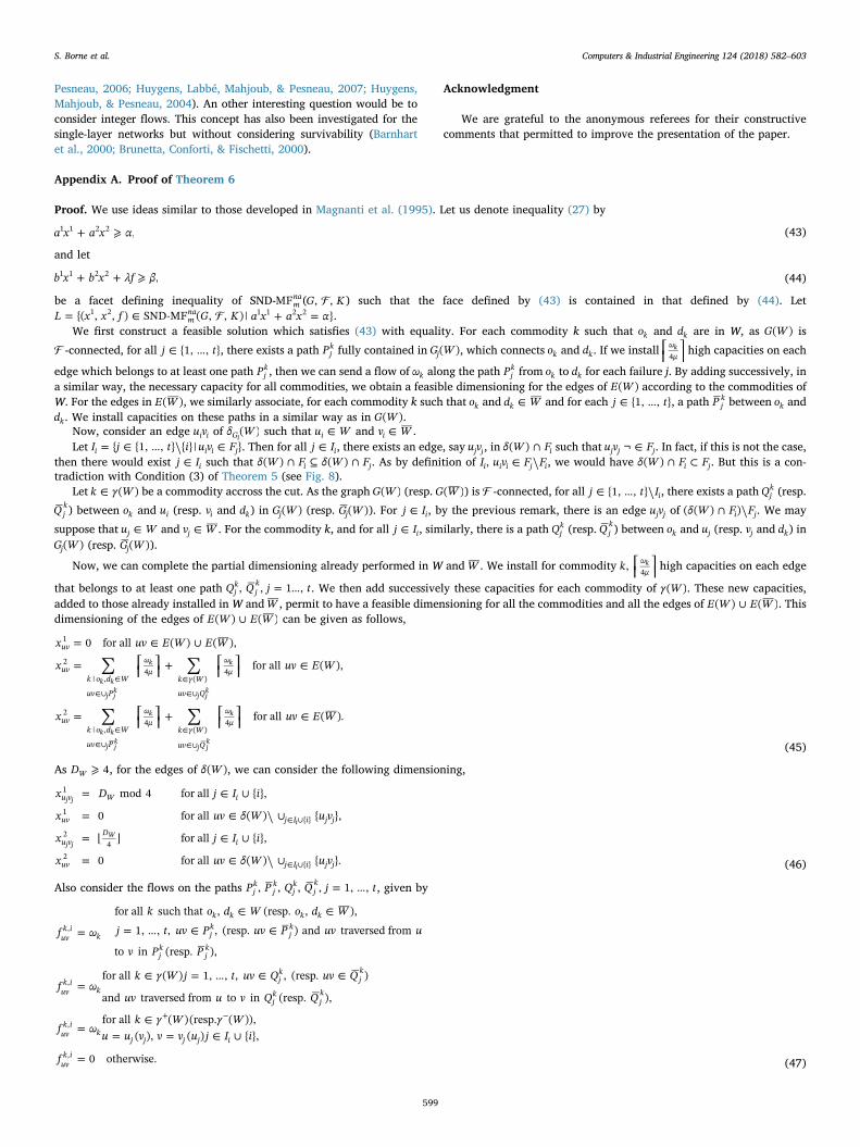
Pesneau, 2006; Huygens, Labbé, Mahjoub, & Pesneau, 2007; Huygens,Mahjoub, & Pesneau, 2004). An other interesting question would be toconsider integer flows. This concept has also been investigated for thesingle-layer networks but without considering survivability (Barnhartet al., 2000; Brunetta, Conforti, & Fischetti, 2000).

Acknowledgment

We are grateful to the anonymous referees for their constructivecomments that permitted to improve the presentation of the paper.

Appendix A. Proof of Theorem 6

Proof. We use ideas similar to those developed in Magnanti et al. (1995). Let us denote inequality (27) by

+ ⩾a x a x α,1 1 2 2 (43)

and let

+ + ⩾b x b x λf β,1 1 2 2 (44)

be a facet defining inequality of SND-MFmna( �G K, , ) such that the face defined by (43) is contained in that defined by (44). Let

�= ∈L x x f G K{( , , ) SND-MF ( , , ) |mna1 2 + =a x a x α}1 1 2 2 .

We first construct a feasible solution which satisfies (43) with equality. For each commodity k such that ok and dk are in W, as G W( ) is

� -connected, for all ∈ …j t{1, , }, there exists a path Pjk fully contained in G W( )j , which connects ok and dk. If we install⎡

⎢⎤⎥

ωμ4k high capacities on each

edge which belongs to at least one path Pjk, then we can send a flow of ωk along the path Pj

k from ok to dk for each failure j. By adding successively, ina similar way, the necessary capacity for all commodities, we obtain a feasible dimensioning for the edges of E W( ) according to the commodities ofW. For the edges in E W( ), we similarly associate, for each commodity k such that ok and ∈d Wk and for each ∈ …j t{1, , }, a path P j

k between ok anddk. We install capacities on these paths in a similar way as in G W( ).

Now, consider an edge u vi i of δ W( )Gi such that ∈u Wi and ∈v Wi .Let = ∈ … ⧹ ∈I j t i u v F{ {1, , } { } | }i i i j . Then for all ∈j Ii, there exists an edge, say u vj j, in ∩δ W F( ) i such that ¬ ∈u v Fj j j. In fact, if this is not the case,

then there would exist ∈j Ii such that ∩ ⊆ ∩δ W F δ W F( ) ( )i j. As by definition of ∈ ⧹I u v F F,i i i j i, we would have ∩ ⊂δ W F F( ) i j. But this is a con-tradiction with Condition (3) of Theorem 5 (see Fig. 8).

Let ∈k γ W( ) be a commodity accross the cut. As the graph G W( ) (resp. G W( )) is � -connected, for all ∈ … ⧹j t I{1, , } i, there exists a path Qjk (resp.

Q jk) between ok and ui (resp. vi and dk) in G W( )j (resp. G W( )j ). For ∈j Ii, by the previous remark, there is an edge u vj j of ∩ ⧹δ W F F( ( ) )i j. We may

suppose that ∈u Wj and ∈v Wj . For the commodity k, and for all ∈j Ii, similarly, there is a path Qjk (resp. Q j

k) between ok and uj (resp. vj and dk) inG W( )j (resp. G W( )j ).

Now, we can complete the partial dimensioning already performed in W and W . We install for commodity ⎡⎢

⎤⎥

k, ωμ4k high capacities on each edge

that belongs to at least one path = …Q Q j t, , 1 ,jk

jk . We then add successively these capacities for each commodity of γ W( ). These new capacities,

added to those already installed in W and W , permit to have a feasible dimensioning for all the commodities and all the edges of ∪E W E W( ) ( ). Thisdimensioning of the edges of ∪E W E W( ) ( ) can be given as follows,

∑ ∑

∑ ∑

= ∈ ∪

= ⎡⎢

⎤⎥+ ⎡

⎢⎤⎥

∈

= ⎡⎢

⎤⎥+ ⎡

⎢⎤⎥

∈

∈

∈∪

∈

∈∪

∈

∈∪

∈

∈∪

x uv E W E W

x uv E W

x uv E W

0 for all ( ) ( ),

for all ( ),

for all ( ).

uv

uvk o d W

uv P

ωμ

k γ W

uv Q

ωμ

uvk o d W

uv P

ωμ

k γ W

uv Q

ωμ

1

2

| ,4

( )4

2

| ,4

( )4

k k

j jk

k

j jk

k

k k

j jk

k

j jk

k

(45)

As ⩾D 4W , for the edges of δ W( ), we can consider the following dimensioning,

= ∈ ∪

= ∈ ⧹ ∪

= ⌊ ⌋ ∈ ∪

= ∈ ⧹ ∪

∈ ∪

∈ ∪

x D j I i

x uv δ W u v

x j I i

x uv δ W u v

mod 4 for all { },

0 for all ( ) { },

for all { },

0 for all ( ) { }.

u v W i

uv j I i j j

u vD

i

uv j I i j j

1

1{ }

24

2{ }

j j

i

j jW

i (46)

Also consider the flows on the paths = …P P Q Q j t, , , , 1, ,jk

jk

jk

jk , given by

=

∈ ∈

= … ∈ ∈

=∈ = … ∈ ∈

=∈

= = ∈ ∪

=

+ −

f ω

k o d W o d W

j t uv P uv P uv u

v P P

f ωk γ W j t uv Q uv Q

uv u v Q Q

f ωk γ W γ W

u u v v v u j I i

f

for all such that , (resp. , ),

1, , , , (resp. ) and traversed from

to in (resp. ),

for all ( ) 1, , , , (resp. )

and traversed from to in (resp. ),

for all ( ) (resp. ( )),( ), ( ) { },

0 otherwise.

uvk i

k

k k k k

jk

jk

jk

jk

uvk i

kjk

jk

jk

jk

uvk i

kj j j j i

uvk i

,

,

,

,(47)


599

The solution x x f( , , )1 2 given by (45)–(47) is feasible for SND- �G KMF ( , , )mna .

Let ∈ ∪ ∪ ∩pq E W E W F δ W( ) ( ) ( ( ))i . And let ′ ′ ′x x f( , , )1 2 be the solution such that

′ = ≠′ = +

′ =′ =

x x uv pqx x

x xf f

for all ,1,

,.

uv uv

pq pq

1 1

1 1

2 2

Clearly, ′ ′ ′x x f( , , )1 2 is feasible for SND- �G KMF ( , , )mna . Furthermore, x x f( , , )1 2 and ′ ′ ′x x f( , , )1 2 satisfy inequality (43) with equality. In consequences,

both solutions satisfy inequality (44) with equality. This yields =b 0pq1 . Similarly, one can show that =b 0pq

2 . As pq is an arbitrary edge of∪ ∪ ∩E W E W F δ W( ) ( ) ( ( ))i , we then have = =b b 0uv uv

1 2 for all ∈ ∪ ∪ ∩uv E W E W F δ W( ) ( ) ( ( ))i .Now, consider the edge u vi i (introduced above) and the solution ∼ ∼ ∼x x f( , , )1 2 such that

= +

= ∈ ≠= −

= ∈ ≠

=

∼

∼∼

∼∼

x x

x x uv E uv u vx x

x x uv E uv u v

f f

4,

for all such that ,1,

for all such that ,

.

u v u v

uv uv i i

u v u v

uv uv i i

1 1

1 1

2 2

2 2

i i i i

i i i i

The solution ∼ ∼ ∼x x f( , , )1 2 is defined from x x f( , , )1 2 by replacing a high capacity on u vi i by 4 small ones. Hence, this solution is feasible. Furthermore, as∼ ∼ ∼x x f( , , )1 2 satisfies (43) with equality, it also satisfies (44) with equality. This implies that =b b4 u v u v

1 2i i i i

. As u vi i is an arbitrary edge of δ W( )Gi, we then

get

= ∈ ⧹b b uv δ W F4 for all ( ) .uv uv i2 1

Consider again an edge ∈ ∪ ∪pq E W E W F( ) ( ) i and the solution x x f( , , )1 2 introduced above. Let ′ ∈k K be a commodity and ′ ∈ …j t{1, , } afailure. Consider x x f( , , )1 2 given by

==

= +

= +

= ∈ ⧹ ∈ ∈ …

′ ′ ′ ′

′ ′ ′ ′

x xx x

f f ε

f f ε

f f uv E pq k K j t

,,

,

,

for all { }, for all , for all {1, , },

pqk j

pqk j

qpk j

qpk j

uvk j

uvk j

1 1

2 2

, ,

, ,

, ,

where < <ε0 12 . Note that as the capacity of edge pq is sufficiently big, we have a residual capacity to carry more flow. In consequences, x x f( , , )1 2 is

feasible. Moreover, this solution satisfies inequality (43), and hence (44), with equality. As x x f( , , )1 2 also satisfies (44) with equality, we obtain+ =′ ′ ′ ′λ ε λ ε 0pq

k jqpk j, , implying that = −′ ′ ′ ′λ λpq

k jqpk j, , . As pq is an arbitrary edge of ∪ ∪E W E W F( ) ( ) i, and ′k and ′j are arbitrary in K and … t{1, , }, re-

spectively, we obtain

= − ∈ ∪ ∪ ∈ ∈ …λ λ uv E W E W F k K j tfor all ( ) ( ) , for all and all {1, , }.uvk j

vuk j

i, ,

Now consider again the edge u vi i of ⧹δ W F( ) i. By Condition (5) of Theorem 5, if we consider the solution x x f( , , )1 2 , as u vi i has a sufficiently bigcapacity, we can add more flow on this edge. In a similar way we can show that = −′ ′ ′ ′λ λu v

k jv uk j, ,

i i i i. And as u vi i is chosen arbitrarly in δ W( )Gi , like ′k and ′j

in K and … t{1, , }, we obtain

= − ∈ ∈ ∈ …λ λ uv δ W k K j tfor all ( ), for all and all {1, , }.uvk j

vuk j

G, ,

i

We have then shown that

= − ∈ ∈ ∈ …λ λ uv E k K j tfor all , for all and all {1, , }.uvk i

vuk i, , (48)

We now show that ∑ ∑ +∈ ∈ λ f λ f( )k K uv E uvk j

uvk j

vuk j

vuk j, , , , is a constant for all failure = …j t1, , , by showing that the sum of the coefficients, corre-

sponding to any cycle in the network, equals zero. Let Δ denote the set of cycles in =D V A( , ). Consider a failure ∈ …j t{1, , } and a particular cycle∈ξ Δ. Let = ∑ ∈λ λξ

k ju v ξ uv

k j,( , )

, . We will show that =λ 0ξk j, for all cycle ∈ξ Δ. Call ξ an s-intersection cycle with respect to the cut δ W( )G if ξ contains

exactly s arcs of δ W( )G . Note that s must be even as ξ is a cycle.If ξ is a 0-intersection cycle, then ξ is completely contained inW orW . We suppose w.l.o.g., that ξ is inW. Let ∈k K and x x f( ˇ , ˇ , ˇ )1 2 be the solution

given by

= + ∈ ∈= ∈ ¬ ∈= ∈

= + ∈

= ¬ ∈

= ∈ ∈ … ⧹

x x uv E W u v v u ξx x uv E W u v v u ξx x uv E

f f u v ξ

f f u v ξ

f f u v A h t j

ˇ 1 for all ( ) such that ( , ) ou ( , ) ,ˇ for all ( ) such that ( , ) ou ( , ) ,ˇ for all ,

ˇ 1 for all ( , ) ,

ˇ for all ( , ) ,

ˇ for all ( , ) , for all {1, , } { }.

uv uv

uv uv

uv uv

uvk j

uvk j

uvk j

uvk j

uvk h

uvk h

1 1

1 1

2 2

, ,

, ,

, ,


600

Here, we construct solution x x f( ˇ , ˇ , ˇ )1 2 from solution x x f( , , )1 2 by installing a small capacity on all the edges in ξ and by sending an additional unit offlow on ξ . Solution x x f( ˇ , ˇ , ˇ )1 2 is still feasible and satisfies (43) with equality. Hence x x f( ˇ , ˇ , ˇ )1 2 satisfies (44) with equality, and in consequence we get

∑ ∑ ∑− + − =∈ ∈ ∈

b x b x λ f λ fˇ ( ) 0.uv E W

uv uvuv E W

uv uvu v ξ

uvk j

uvk j

vuk j

vuk j

( )

1 1

( )

1 1

( , )

, , , ,

As =b 0uv1 for all ∈uv E W( ), we obtain∑ − =∈ λ 0u v ξ uv

k j( , )

, , and then =λ 0ξk j, . As cycle ξ , the commodity k and the failure j are arbitrary, we have then

shown that

= ∈ ∈

∈ …

λ ξ k K

j t

0 for all 0-intersection cycle Δ, for all

and for all {1, , }.ξk j,

(49)

Now suppose that ξ is a 2-intersection cycle. Assume that p p( , ) and q q( , ) are the cutset arcs belonging to ∩δ W ξ( )G with ∈p q W, and∈p q W, .

If =p q and =p q , then ξ can be decomposed into three cycles: a 0-intersection cycle denoted by ξ1 contained in W, a 0-intersection cycledenoted by ξ2 contained in W and a cycle formed by the arcs p p( , ) and =p p q q( , ) ( , ). We then have = + + +λ λ λ λ λξ

k jξk j

ξk j

ppk j

p pk j, , , , ,

1 2. As ξ1 and ξ2 are

0-intersection cycles, = =λ λ 0ξk j

ξk j, ,

1 2and by (48), we have = −λ λpp

k jp pk j, , . Thus =λ 0ξ

k j, .Now suppose that ≠pp qq and one of the two edges pp or qq belongs to Fi. We suppose, w.l.o.g., that ∈qq Fi and ¬ ∈pp Fi. Let pp be the edge

which belongs to δ W( )Gi. One can construct a feasible solution x x f( , , )1 2 in a similar way as x x f( , , )1 2 (given above for the edge u vi i). Remark that

=x Dpp W1 mod 4 and = ⌊ ⌋xpp

D24W . Consider the solution obtained from x x f( , , )1 2 by installing a small capacity on all the edges of

∩ ∪ ∪ξ E W E W F( ( ) ( ) )i , and by sending ε units of flow on ξ (for a certain >ε 0). The additional flow is possible since by Condition (5) of Theorem 5,there is a positive residual capacity on the edge pp . This new solution is feasible. As both solutions satisfy (43) with equality and hence (44), we get

=λ 0ξk j, .

If =pp qq and ¬ ∈pp qq F, i, we define a solution x x f( , , )1 2 by considering for the edges of the cut δ W( )Gi the following values

=

= ∈

= ⌊ ⌋−

=

= ∈ ⧹

x D

x uv δ W

x

x

x uv δ W pp qq

mod 4,

0 for all ( ),

1,

1,

0 for all ( ) { , }.

pp W

uv G

ppD

qq

uv G

1

1

24

2

2

i

W

i

For the dimensioning of E W( ) and E W( ), we suppose that we have installed a sufficient capacity which permits to carry the flows of the commoditiesin W and W on the paths fully contained in G W( ) and G W( ). These capacities can be taken as big as we want. So, by Condition (5) of Theorem 5, thecommodities of γ W( ) can be routed in such a way that pp and qq contain at least ε (for a certain ε >0) units of residual capacity. This solution isfeasible and satisfies (43) and then (44) with equality. Using the residual capacity ε on pp and qq , one can obtain a new feasible solution fromx x f( , , )1 2 by adding an additional flow ε along ξ for commodity k, and installing a small capacity on the edges of ξ not in δ W( )Gi . This new solution isalso feasible and satisfies (43) and (44) as equalities. As commodity ∈k K , the failure ∈ …j t{1, , } and the 2-intersection cycle ∈ξ Δ are arbitrary,we have that

= ∈ ∈

∈ …

λ ξ k K

j t

0 for all 2-intersection cycle Δ, for all


(50)

Now consider an arbitrary s-intersection cycle ξ . Let k be a commodity and j be a failure. Let ξ be the cycle given by …s s s s s s{( , ), ( , ), , ( , )}T1 2 2 3 1 with∈s W1 . Let s s( , )t t1 2

be the first arc of the cycle ξ that crosses δ W( ) and s s( , )t t3 4the first subsequent arc that re-enters set W. Note that cycle

′ = …ξ s s s s s s{( , ), , ( , ), ( , )}t t t t t t1 2 3 4 4 1is a 2-intersection cycle. We then have =′⧹λ λξ s s

k js sk j

( , ), ,

t t t t1 4 1 4. So, we can replace the path ′⧹ξ s s( , )t t1 4

by the arc s s( , )t t1 4.

Repeating this argument, one can construct a 0-intersection cycle ψ that satisfies =λ λξk j

ψk j, , . As k and j are arbitrary, we obtain that

= ∈ ∈

∈ …

λ ξ k K

j t

0 for all cycle Δ, for all


(51)

We have shown that ∑ ∑ +∈ ∈ λ f λ f( )k K uv E uvk j

uvk j

vuk j

vuk j, , , , is a constant, say λj, for any failure ∈ …j t{1, , }.

We can now show that =b ρuv1 1 and =b ρuv

2 2 for all ∈uv δ W( )Gi . Consider the solution x x f( , , )1 2 given in the beginning of the proof, an edge∈pq δ W( )Gi

such that ≠pq u vi i, a commodity ′ ∈k K and a failure ∈ …j t{1, , }. Let P u p( , )i be a path from node ui to p fully contained in W andP q v( , )i a path from q to vi in W . Consider the solution x x f(¨ , ¨ , ¨)1 2 such that

= − = −

=

= ∈ ⧹

= + ∈ ∪= ∈ ∪ ⧹ ∪

= ∈

x x D

x

x x uv δ W u v pq

x x u v P u p P q vx x u v E W E W P u p P q v

x x uv E

¨ 1 mod 4 1,

¨ 1,

¨ for all ( ) { , },

¨ 1 for all ( , ) ( , ) ( , ),¨ for all ( , ) ( ) ( ) ( ( , ) ( , )),

¨ for all .

u v u v W

pq

uv uv G i i

uv uv i i

uv uv i i

uv uv

1 1

1

1 1

1 1

1 1

2 2

i i i i

Define the flows as follows.


601

= + ∈ ∪

= −

=

= ∈ ⧹ ∪ ∪

= ∈ ∈ ⧹ ′ ∈ … ⧹

′ ′

′ ′

′

′ ′

f f u v P u p P q v

f f

f

f f uv E P u p P q v u v pq

f f uv E k K k h t j

¨ 1 for all ( , ) ( , ) ( , ),

¨ 1,

¨ 1,

¨ for all ( ( , ) ( , ) { , }),

¨ for all , for all { }, for all {1, , } { }.

uvk j

uvk j

i i

u vk j

u vk j

pqk j

uvk j

uvk j

i i i i

uvk h

uvk h

, ,

, ,

,

, ,

, ,

i i i i

Solutions x x f( , , )1 2 and x x f(¨ , ¨ , ¨)1 2 are feasible and satisfy constraint (43) with equality. In consequence, they also satisfy (44) with equality. Thisimplies that

∑ ∑ ∑− − − − + − =∈ ∪ ∈

′

∈

′ ′ ′b b ρ λ λ λ λ 0.u v pquv P u p P q v

uvu v P u p

uvk j

u v P q vuvk j

u vk j

pqk j1 1

( , ) ( , )

1

( , ) ( , )

,

( , ) ( , )

, , ,i i

i i i ii i

As =b 0uv1 for all ∈ ∪uv E W E w( ) ( ) and by (48) = −′ ′λ λu v

k jv uk j, ,

i i i i, we have

∑ ∑− − − − − =∈

′ ′

∈

′ ′b b λ λ λ λ 0.u v pqu v P u p

uvk j

pqk j

u v P q vuvk j

v uk j1 1

( , ) ( , )

, ,

( , ) ( , )

, ,i i

i ii i

As P u p pq P q v( , ), , ( , )i i and v ui i form a cycle, we have − =b b 0u v pq1 1i i

. As pq was chosen arbitrarily, we obtain =b ρuv1 1 for all ∈uv δ W( )Gi

for ∈ρ IR1 .Since =b b4uv uv

2 1 for all ∈uv δ W( )Gi, we have also =b ρ4uv

2 1 for all ∈uv δ W( )Gi.

Thus, inequality (44) is equivalent to

∑+ + ==

ρ x δ W ρ x δ W λ λ( ( )) 4 ( ( )) ,G Gj

t

j1 1 1 2

1i i

which implies that

+ = ′ρ x δ W ρ x δ W λ( ( )) 4 ( ( ))G G1 1 1 2

i i

where ′ = −∑ =λ λ λjt

j1 . As the face defined by inequality (44) is not empty, ≠ρ 01 and we obtain that

+ =′= □x δ W x δ W λ

ρD( ( )) 4 ( ( )) .G G W

1 21i i

References

Ahuja, R. K., Magnanti, T. L., & Orlin, J. (1993). Network flows: Theory, algorithms, andapplications. Englewood Cliffs, NJ: Prentice Hall.

Barahona, F. (1996). Network design using cut inequalities. SIAM Journal of Optimization,6, 823–837.

Barahona, F., & Mahjoub, A. R. (1995). On two-connected subgraph polytopes. DiscreteMathematics, 147, 19–34.

Barnhart, C., Hane, C. A., & Vance, P. (2000). Using branch-and-price-and-cut to solveorigin-destination integer multicommodity flow problem. Operations Research, 48,318–326.

Barnhart, C., Johnson, E. L., Nemhauser, G. L., Savelsbergh, M. W. P., & Vance, P. H.(1998). Branch-and-Price: Column generation for solving huge integer programs.Operations Research, 46, 316–329.

Bigos, W., Cousin, B., Gosselin, S., Foll, M. L., Nakajima, H. (2007). Survivable MPLS overoptical transport networks: Cost and resource usage analysis. IEEE Journal on SelectedAreas in Communications.

Binh, H. T. T., & Ly, H. D. (2012). Genetic algorithm for solving multilayer survivableoptical network design problem. International Journal of Machine Learning andComputing, 2(6), 812–816.

Borne, S. (2006). Sécurisation et dimensionnement de réseaux multicouches: modèles etpolyèdres. Ph.D. thesis. Clermont-Ferrand, France: Université Blaise Pascal.

Borne, S., Gabrel, V., Mahjoub, A. R., Taktak, R. (2011). Multilayer survivable opticalnetwork design. In Proceedings of INOC 2011, Lecture Notes in Computer Science (Vo.6701, pp. 170–175).

Borne, S., Gourdin, E., Liau, B., & Mahjoub, A. R. (2006). Design of survivable IP-over-Optical networks. Annals of Operation Research, 146, 41–73.

Bradner, S. (1995). The Recommendation for the IP Next Generation Protocol, IETF(RFC1752).

Brunetta, L., Conforti, M., & Fischetti, M. (2000). A polyhedral approach to an integermulticommodity flow problem. Discrete Applied Mathematics, 101, 13–36.

Dahl, G., Huygens, D., Mahjoub, A. R., & Pesneau, P. (2006). On the k -edge-disjoint 2-hop-constrained paths polytope. Operations Research Letters, 34, 577–582.

Dahl, G., & Stoer, M. (1998). A cutting plane algorithm for multicommodity survivablenetwork design problems. SIAM Journal on Computing, 10, 1–11.

Elf, M., Gutwenger, C., Jünger, M., Rinaldi, G. (2001). Branch-and-Cut Algorithms forCombinatorial Optimization and Their Implementation in ABACUS. In M. Jünger, D.Naddef (Eds.), Computational Combinatorial Optimization, Lecture Notes in ComputerScience (vol. 2241, pp. 157–222).

Fortz, B., McCormick, T., Mahjoub, A. R., & Pesneau, P. (2006). Two-edge connectedsubgraphs with bounded rings: Polyhedral results and Branch-and-Cut. MathematicalProgramming, 105, 85–111.

Fortz, B., & Poss, M. (2009). An improved Benders decomposition applied to a multi-layernetwork design problem. Operations Research Letters, 37(5), 359–364.

Ghani, N., Liu, Q., Gumaste, A., Benhaddou, D., Rao, N. S. V., & Lehman, T. (2008).Control plane design in multi-domain/multi-granularity optical networks. IEEECommunications Magazine, 46(6), 78–87.

Goldberg, A. V., & Tarjan, R. E. (1988). A new approach to the maximum-flow problem.Journal of the Association for Computing Machinery, 35, 921–940.

Gomory, R. E., & Hu, T. C. (1961). Multi-terminal network flows. SIAM Journal on AppliedMathematics, 9, 551–570.

Gouveia, L., Patrício, P., de Sousa, A., Valadas, R. (2003). MPLS over WDM networkdesign with packet level QoS constraints based on ILP models. In Proceedings IEEEINFOCOM 2003San Francisco.

Gouveia, L., Patrício, P., & de Sousa, A. (2008). Hop-constrained node survivable networkdesign: An application to MPLS over WDM. Networks and Spatial Economics, 8, 3–21.

Grötschel, M., Monma, C. L., & Stoer, M. (1995). Design of survivable networks.Handbooks in OR & MS, 7, 617–671 Ball MO et al. (Eds.).

Gusfield, D. (1990). Very simple methods for all pairs network flow analysis. SIAMJournal on Computing, 19, 143–155.

Huygens, D., Labbé, M., Mahjoub, A. R., & Pesneau, P. (2007). Two edge-disjoint hop-constrained paths: Valid inequalities and branch-and-cut. Networks, 49, 116–133.

Huygens, D., Mahjoub, A. R., & Pesneau, P. (2004). Two edge hop-constrained paths andpolyhedra. SIAM Journal on Discrete Mathematics, 18, 287–312.

Jensen, T. (2001). Internet protocol and transport protocols. Telektronikk, 97, 20–38.Kerivin, H. (2000). Réseaux fiables et polyèdres. Ph.D. thesis. Clermont-Ferrand, France:

Université Blaise Pascal.Kerivin, H., & Mahjoub, A. R. (2005). Design of survivable networks: A survey. Networks,

46, 1–21.Knippel, A., & Lardeux, B. (2007). The multi-layered network design problem. European

Journal of Operations Research, 183, 87–99.Koster, A. M. C. A., Orlowski, S., Raack, C., Baier, G., & Engel, T. (2008). Single-layer cuts

for multi-layer network design problems, telecommunications modeling, policy, andtechnology. Operations Research/Computer Science Interfaces Series, 44, 1–24Raghavan S, Golden Bruce L, Wasil Edward A (Eds.).

Lardeux, B. (2005). Conception de réseaux de Télécommunications Multicouches etEvolutifs. Ph.D. thesis. France: Université Technologique de Compiègne.

Lübbecke, M. E., Desrosiers, J. (2004). Selected topics in column generation, TechnicalReport G-2002-64 GERAD.


602

http://refhub.elsevier.com/S0360-8352(18)30252-3/h0005






















































Magnanti, T. L., Mirchandani, P., & Vachani, R. (1993). The convex hull of two corecapacitated network design problems. Mathematical Programming, 60, 233–250.

Magnanti, T. L., Mirchandani, P., & Vachani, R. (1995). Modeling and solving the two-facility capacitated network loading problem. Operations Research, 43, 142–157.

Mahjoub, A. R. (1994). Two-edge connected spanning subgraphs and polyhedra.Mathematical Programming, 64, 199–208.

Mattia, S. (2013). A polyhedral study of the capacity formulation of the multilayer net-work design problem. Networks, 62, 17–26.

Orlowski, S., Wessäly, R. (2004). An integer programming model for multi-layer networkdesign, ZIP report ZR-04-49.

Orlowski, S., Koster, A. M. C. A., Raak, C., Wessäly, R. (2006). Two-layer network designby branch-and-cut featuring mip-based heuristics, ZIP report ZR-06-47.

Pacharintanakul, P., Tipper, D. (2009). The Effects of Multi-Layer Traffic on theSurvivability of IP-over-WDM Networks. In Proc. of IEEE ICC ’09. International con-ference on communications Germany.

Postel, J. (1981a). Internet Control Message Protocol. DARPA Internet Program ProtocolSpecification, IETF (RFC792).

Postel, J. (1981b) Internet Protocol. DARPA Internet Program Protocol Specification,IETF (RFC791).

Postel, J. (1981c). Transmission Control Protocol. DARPA Internet Program Protocol

Specification, IETF (RFC793).Reilly, W. J. (1931). The law of retail gravitation. New York: Knickerbocker Press.Reinelt, G. (1991). TSPLIB – a traveling salesman problem library. ORSA Journal on

Computing, 3, 376–384.Ricciato, F., Salsano, S., Belmonte, A., Listanti, M. (2002). Off-line configuration of a

MPLS over WDM network under time-varying offered traffic. In Proceedings IEEEINFOCOM.

Ruiz, M., Pedrola, O., Velasco, L., Careglio, D., Fernández-Palacios, J., & Junyent, G.(2011). Survivable IP/MPLS-Over-WSON multilayer network optimization. IEEE/OSAJournal of Optical Communications and Networking, 3, 629–640.

Schrijver, A. (2003). Combinatorial optimization: Polyhedra and efficiency, algorithms andcombinatorics, vol. 24. Springer.

Stoer, M. (1992). Design of survivable networks. Lectures Notes in Mathematics, 1531.Thienel, S. (1995). ABACUS – A Branch-And-CUt System. Ph.D. thesis. Universität zu

Köln.Voge, M.E. (2006). Optimisation des réseaux de télécommunications: Réseaux multi-

niveaux, Tolérance aux pannes et surveillance de traffic, Ph.D. thesis. France:Université de Sophia-Antipolis.

Zouganeli, E. (2001). Optical network functionality: From “Dumb Fat Pipes” to brightnetworking. Telektronikk, 97, 346–354.


603




















Documents

Computers & Industrial Engineering