Embed Size (px)
Citation preview

APPROVED: Vijay Vaidyanathan, Major Advisor Ram Dantu, Committee Member Joao Cangussu, Committee Member Kasturi Narayanan, Committee Member Albert B Grubbs, Committee Member and Chair of
the Department of Engineering Technology Oscar N. Garcia, Dean of the College of
Engineering Sandra L. Terrell, Dean of the Robert B. Toulouse
School of Graduate Studies
COMPUTER VIRUS SPREAD CONTAINMENT USING FEEDBACK CONTROL
Arun Yelimeli Guruprasad, B.E.
Thesis Prepared for the Degree of
MASTER OF SCIENCE
UNIVERSITY OF NORTH TEXAS
December 2004

Yelimeli Guruprasad, Arun. Computer virus spread containment using feedback control. Master
of Science (Engineering Technology), December 2004, 53 pp., 1 table, 25 figures, references, 31
titles.
In this research, a security architecture based on the feedback control theory has been
proposed. The first loop has been designed, developed and tested. The architecture proposes a
feedback model with many controllers located at different stages of network. The controller at each
stage gives feedback to the one at higher level and a decision about network security is taken.
The first loop implemented in this thesis detects one important anomaly of virus attack, rate of
outgoing connection. Though there are other anomalies of a virus attack, rate of outgoing connection
is an important one to contain the spread. Based on the feedback model, this symptom is fed back and
a state model using queuing theory is developed to delay the connections and slow down the rate of
outgoing connections. Upon implementation of this model, whenever an infected machine tries to
make connections at a speed not considered safe, the controller kicks in and sends those connections
to a delay queue. Because of delaying connections, rate of outgoing connections decrease. Also
because of delaying, many connections timeout and get dropped, reducing the spread.
PID controller is implemented to decide the number of connections going to safe or suspected
queue. Multiple controllers can be implemented to control the parameters like delay and timeout.
Control theory analysis is performed on the system to test for stability, controllability, observability.
Sensitivity analysis is done to find out the sensitivity of the controller to the delay parameter.
The first loop implemented gives feedback to the architecture proposed about symptoms of an
attack at the node level. A controller needs to be developed to receive information from different
controllers and decision about quarantining needs to be made. This research gives the basic
information needed for the controller about what is going on at individual nodes of the network. This
information can also be used to increase sensitivity of other loops to increase the effectiveness of
feedback architecture.
ii
Copyright 2004
by
Arun Yelimeli Guruprasad
iii
ACKNOWLEDGMENTS
I express my gratitude and thanks to my advisor and major professor Dr. Vijay
Vaidyanathan for his support, confidence, encouragement and guidance throughout my graduate
program and in completing this thesis.
I thank my supervisor Dr. Ram Dantu for his ideas, encouragement, attention to detail,
and excellent guidance that have been necessary for this thesis.
I thank my committee member Dr. Joao Cangussu for his supply of knowledge, technical
support and friendly guidance.
I thank the Dr. Albert B. Grubbs, Chair of Engineering Technology Department,
University of North Texas, for his support and encouragement all along my graduate studies.
I express my gratitude to my Industrial representative Mr. Kasturi Narayanan for his time
and support.
I thank my parents Mr. Guruprasad Yelimeli and Mrs. Rathna Prasad for their love,
patience and support throughout my graduate studies and also like to thank my brother Mr. Kiran
Yelimeli and Sister-in-law Sindhu KiranKumar for their support and encouragement.
I would also like to thank my friends Sriteja Tarigopula, Anand Ale, Mehul Baxi and
Umashankar Baburajan for their help, suggestions and their valuable time.
iv
TABLE OF CONTENTS Page
ACKNOWLEDGMENTS ............................................................................................................. iii LIST OF TABLES AND FIGURES.............................................................................................. vi INTRODUCTION .......................................................................................................................... 1
Existing Defenses........................................................................................................................ 2
Intrusion Detection Systems ................................................................................................... 2
Firewalls.................................................................................................................................. 2
Honey Pots .............................................................................................................................. 3
Statement of the Problem............................................................................................................ 3
Purpose of the Study ................................................................................................................... 3 REVIEW OF LITERATURE ......................................................................................................... 5
Recent Worms and Techniques Used to Spread Them............................................................... 5
Code Red 1.............................................................................................................................. 5
Code Red II ............................................................................................................................. 5
Nimda...................................................................................................................................... 5
Slammer/Sapphire................................................................................................................... 6
How Slammer Works.......................................................................................................... 6
Response to Sapphire’s Spread........................................................................................... 7
Distributed Denial of Service Attacks .................................................................................... 9
“Better” Worms - Theory............................................................................................................ 9
Hit List Scanning .................................................................................................................. 10
Permutation Scanning ........................................................................................................... 10
Topological Scanning ........................................................................................................... 10
Flash Worms ......................................................................................................................... 11
Control Systems ........................................................................................................................ 11
Open Loop Control System .................................................................................................. 12
Closed Loop Control System................................................................................................ 13
The Three-Term Controller................................................................................................... 13
The Characteristics of P, I, and D Controllers ...................................................................... 15
Previous Work .......................................................................................................................... 15
v
EXPERIMENTAL SETUP AND PROCEDURE ........................................................................ 17
System Architecture.................................................................................................................. 17
Model Description .................................................................................................................... 20
Experimental Setup................................................................................................................... 23
LabVIEW Model ...................................................................................................................... 23
Time to Synchronize Different Loops .................................................................................. 25
Generation and Queuing ....................................................................................................... 27
Safe Connections .................................................................................................................. 29
Delaying Suspected Connections.......................................................................................... 30
PID Controller....................................................................................................................... 31
Simulink Validation.............................................................................................................. 33 RESULTS AND DISCUSSIONS................................................................................................. 34
Total Connections ..................................................................................................................... 34
Acceleration .............................................................................................................................. 35
Total Input Connections............................................................................................................ 36
Delay ......................................................................................................................................... 37
LabVIEW Implementation........................................................................................................ 38
Controllability & Observability ................................................................................................ 41
Settling Time............................................................................................................................. 42
Sensitivity Analysis .................................................................................................................. 44
Limitations ................................................................................................................................ 45 CONCLUSIONS........................................................................................................................... 47 FUTURE WORK.......................................................................................................................... 49 REFERENCES ............................................................................................................................. 51

vi
LIST OF TABLES AND FIGURES
Table 1 Relationship between different PID gains, rise time, overshoot, settling time and steady state error. (Source: 1997, Regents of the University of Michigan, CTM tutorial, PID tutorial, reprinted with permission.) ..................................................... 15
Figure 1 Aggregate scans per second in first 5 minutes (Sapphire) [4] ..................................... 8
Figure 2 Aggregate scans per second in first 12 hours (Sapphire) [4]....................................... 8
Figure 3 State Model................................................................................................................ 12
Figure 4 Open loop control system .......................................................................................... 13
Figure 5 Closed loop control system........................................................................................ 13
Figure 6 Feedback controller ................................................................................................... 14
Figure 7 Controller architecture for end-to-end security engineering ..................................... 18
Figure 8 Model for connections accepted, delayed and rejected for parametric control ......... 20
Figure 9 Front panel of LabVIEW client ................................................................................. 24
Figure 10 Timer Loop for synchronous operation of all the loops ............................................ 25
Figure 11 Simulation of attack and queuing .............................................................................. 27
Figure 12 Makes outgoing connections from safe queue........................................................... 29
Figure 13 Delaying suspected connections and adding them back to safe queue; also dropping timed out connections ................................................................................................ 30
Figure 14 Feedback loop with PID controller............................................................................ 31
Figure 15 Simulink model with a PID controller and the State Variable model ....................... 33
Figure 16 Behavior of the state model for the control of the number of connections on the presence of a worm spreading according to an S-shape function. (a) Shows the total number of connections with and without feedback ................................................... 34
Figure 17 Acceleration of outgoing connections for better detection times .............................. 35
Figure 18 Number of connections on the delayed queue........................................................... 36
Figure 19 Result of application of the feedback loop approach at the host and at the firewall level............................................................................................................................ 37
Figure 20 State model implemented .......................................................................................... 38
Figure 21 Experimental result for Kp= 1, Ti = 0.01, Td = 0 & set point = 20, where time is in seconds and y-axis is number of connections per second.......................................... 40
Figure 22 Experimental result for Kp = 1.5, Ti = 0 & Td = 5 ................................................... 41
Figure 23 Relation between Integral time constant and settling time........................................ 43
Figure 24 Graph showing relation between proportional constant and settling time ................ 43
Figure 25 Sensitivity of the number of connections sent directly to the safe queue as the delay parameter changes ..................................................................................................... 45

1
INTRODUCTION
Computer virus is a software program, which harms a computer when infected [1].
General tendency observed over the period is that a person who writes such programs would like
to harm as many systems as possible. In early days (before computer networks) virus
programmers used disk media (ex: floppy) to spread the virus to as many systems as possible.
Computer virus is defined as “A parasitic program written intentionally to enter a
computer without the user's permission or knowledge. The word parasitic is used because a virus
attaches to files or boot sectors and replicates itself, thus continuing to spread. Though some
viruses do little but replicate, others can cause serious damage or affect program and system
performance. A virus should never be assumed harmless and left on a system." [31].
Research has been going on to reduce the spread of viruses to minimize the destruction
caused by them. Viruses can be broadly categorized into the following categories:
• Viruses - A virus is a small piece of software that attaches to real programs. For example, a virus might attach itself to a program such as a spreadsheet program. Each time the spreadsheet program runs, the virus runs, too, and it has the chance to reproduce (by attaching to other programs) or wreak havoc [28].
• E-mail viruses - e-mail virus moves around in e-mail messages, and usually replicates itself by mailing itself to dozens of people in the victim's e-mail address book [28].
• Worms - A worm is a small piece of software that uses computer networks and security holes to replicate itself. A copy of the worm scans the network for another machine that has a specific security hole. It copies itself to the new machine using the security hole, and then starts replicating from there, as well [28].
• Trojan horses - A Trojan horse is simply a computer program. The program claims to do one thing (it may claim to be a game) but instead does damage when you run it (it may erase your hard disk). Trojan horses have no way to replicate automatically [28].
In the past active worms have taken hours if not days to spread effectively. This gives
sufficient time for humans to recognize the threat and limit the potential damage. This is not the
case anymore. Modern viruses spread very quickly. Damage caused by modern computer viruses

2
(example - Code Red, Sapphire and Nimda) is greatly enhanced by the rate at which they spread.
Most of these viruses have an exponential spreading pattern. Future worms will exploit
vulnerabilities in software systems that are not known prior to the attack. Neither the worm nor
the vulnerabilities they exploit will be known before the attack and thus spread of these viruses
cannot be prevented by software patches or antiviral signatures [1].
Existing Defenses
There are a variety of network components in the market today that protect machines
from different kinds of worms. Network perimeter is primary concern for security managers.
Security managers have focused on multiple security components to keep their networks safe.
Examples are: Antivirus, Firewalls, Intrusion Detection Systems, and Honey Pots.
Intrusion Detection Systems
Network Intrusion Detection Systems examine the network traffic and host intrusion
systems detect outsider infiltration as well as unauthorized access by users who are trusted
insiders. Intrusions are characterized into network traffic patterns that are suspicious and these
are called signatures. These signatures are compared against the network traffic patterns and
deviation generates security alerts. But these alerts can be false alarms. Due to nature of the
signatures, these systems can be as accurate as the signatures themselves. Moreover, these
systems are reactive and cannot prevent the attacks [5].
Firewalls
Firewalls often only have the packet filter rules applied or are used to protect just one
server, such as external Web server. Hence most of these firewall rules are static and cannot
respond to dynamic changes [5].

3
Honey Pots
Honey pots lure attackers by presenting a more visible and apparently vulnerable
resource than the enterprise network itself. These are also useful for forensics. But these can be
vulnerable themselves because they attract attackers’ special attention. Also if they are
incorrectly configured, they make network more vulnerable [5].
Thus, firewalls, routers, Intrusion Detection Systems, and Honey Pots can be very useful
as elements for network defense but they can not protect the network by themselves. But by
careful integration and engineering of these devices, security level can be increased [5].
Statement of the Problem
It is difficult to control or stop the unknown computer worms that spread very fast.
Modern day viruses spread in milliseconds. They cannot be controlled with existing technologies
which are either signature based or too slow to control the spread and damage caused by
unknown fast spreading worms, such as Slammer, Code Red, Nimda etc.
Purpose of the Study
Purpose of the study is to
• Develop and simulate a state model to contain the rate of outgoing connections made by a compromised system.
• Implement and test the state model using LabVIEW® (National Instrument Corporation, Austin, Texas, www.ni.com).and implement feedback control using PID (Proportional Integral Derivative) controller
• Perform stability, controllability, observability and sensitivity analysis on the implemented control system.
Objectives of this research are to design an architecture based on classical feedback
control to: (1) detect worm-based threats; (2) dynamically quarantine infections to localized
sectors to prevent propagation of infection; and (3) develop technologies to automatically and

4
dynamically quarantine these fast spreading worms to a peak infection portion of 1% of
vulnerable machines that would otherwise infect approximately 100% of vulnerable machines.

5
REVIEW OF LITERATURE
The model developed is based on the analysis of some popular worms that spread very
fast and caused havoc in the recent history. Below is a brief description of these worms, their
spreading pattern and some of the techniques these worm authors’ use to increase the spread rate.
Recent Worms and Techniques Used to Spread Them
Code Red 1
On July 12, 2001, this worm began to exploit the buffer-overflow vulnerability in
Microsoft® IIS Web servers (Microsoft Corporation, www.microsoft.com). Upon infecting a
machine, the worm checks to see if the date (as kept by the system clock) is between the first and
the nineteenth of the month. If so, the worm generates a random list of IP addresses and probes
each machine on the list in an attempt to infect as many computers as possible [3].
Code Red II
This worm also used the same Microsoft IIS Web server’s buffer overflow vulnerability
as Code Red I. This worm had single stage scanning technique and used a localized scanning
strategy, which made it successful in infecting addresses close to it [3].
Nimda
This worm used multiple ways to spread through the network. This worm is believed to
have used the following five different strategies to spread itself
• Infecting Web servers from infected client machines via active probing for Microsoft IIS vulnerability.
• Bulk emailing of itself as an attachment based on email addresses determined from the infected machine.
• Copying itself across open network shares.
• Adding exploit code to Web pages on compromised servers in order to infect clients that browse the page.

6
• Scanning for the backdoors left behind by Code Red II and also the “sadmind” worm” [3]
Slammer/Sapphire
Slammer's attack was hundreds of times faster than the Code Red virus or Nimda worm.
It started with a single packet. The worm hit its first victim at 12:30 am (January 25 2003)
Eastern standard time. The machine - a server running Microsoft SQL (Structured Query
Language) - instantly sent out millions of Slammer clones, targeting computers at random. By
12:33 am, the number of slave servers in Slammer's replicant army was doubling every 8.5
seconds [28].
How Slammer Works
Slammer owes its speed to UDP (Unreliable Datagram Protocol), an Internet protocol
that's lighter and quicker than the TCP (Transmission Control Protocol used for Web sites, email,
and file downloads). TCP requires sender and receiver to acknowledge each other in a handshake
before exchanging information; UDP can carry a message in a single, one-way packet. Microsoft
SQL Server 2000 software has a UDP-powered directory service that lets applications
automatically find the right database. Moreover, SQL code comes built into other programs the
company sells. Many Slammer victims didn't even realize they were running SQL [28].
The worm takes advantage of a common software bug called a buffer overflow. Buffers
overflow when a data string is written into memory without its length being checked by the
program. If the string is too long, the tail end of the data overwrites the program's own code [28].
The unique intelligent feature of Slammer is how it uses an attack on just one type of
software as leverage for a general attack on the Web itself. Machines infected by the worm
swiftly spam the Network with randomly addressed traffic, hitting other vulnerable servers. As
the number of computers spewing Slammer packets rises, the situation reaches critical mass,

7
potentially creating a denial of service attack on all 4 billion IP (Internet Protocol) addresses on
the Net [28].
Below is a brief description of how Slammer worked and how it could achieve such high
speed spreading, as described in an article from Wired [28].
Get inside: Slammer is a single UDP packet, one that would normally be a harmless request to find a specific database service. The first byte in the string - 04 - tells SQL Server that the data following it is the name of the online database being sought. Microsoft specifies that this name be at most 16 bytes long and end in 00. But in the Slammer packet, the bytes run on, so there is no 00 among them. As a result, the SQL software pastes the whole thing into memory.
Reprogram the machine: The initial string of 01 character spills past the 128 bytes of memory reserved for the SQL Server request and into the computer's stack. The first thing the computer does after opening Slammer's UDP "request" is overwrite its own stack with new instructions that Slammer has disguised as a routine query. The computer reprograms itself without realizing it.
Choose victims at random: Slammer generates a random IP address, targeting another computer that could be anywhere on the Internet. To randomize: It looks up the number of milliseconds that have elapsed on the CPU's system clock since it was booted and interprets the number as an IP address.
Replicate: The envelope is addressed, now it just needs to be stuffed. Slammer points to its own code as the data to send. The infected computer writes out a new copy of the worm and sends the UDP packet.
Repeat: After sending off the first packet, Slammer loops around immediately to send another to a different computer without wasting a single millisecond. Instead of making another call to the system clock to get the time, it just shuffles the bits of the IP address already in memory to create a new one. A home Personal Computer could send a couple hundred copies onto its broadband link every second. Corporate data centers started launching tens of thousands of worms per second. Because it replicated so fast, the worm was able to take down millions more, kicking them offline with a flood of meaningless traffic.
Response to Sapphire’s Spread
Most accurate data was obtained from the University of Wisconsin Advanced Internet
Lab, where all packets into an otherwise unused network (a “tarpit” network) is logged. Many
sites began filtering all the UDP packets with a destination port of 1434. Though filtering
reduced the bandwidth consumed by the infected hosts, it did nothing to limit the spread of the
worm.

8
Figure 1 Aggregate scans per second in first 5 minutes (Sapphire) [4]
Note: Break in the graph above shows transient failure in the data collection approximately 2 minutes and 40 seconds after Sapphire began to spread.
Figure 2 Aggregate scans per second in first 12 hours (Sapphire) [4].

9
The response was so slow that by the time filtering was implemented; the worm had
infected almost all the susceptible hosts [4]. Figure 1 & 2 shows the scanning rate of this virus in
the first five minutes and first twelve hours after the launch of the worm.
Distributed Denial of Service Attacks
This can be described as attempt by an attacker to prevent legitimate users from using
resources. An attacker usually floods the network and steals the bandwidth available to the user.
Some well-known examples of denial of service attacks include
• Attempts to “flood” a network, thereby preventing legitimate network traffic
• Attempts to disrupt connections between two machines, thereby preventing access to a service.
• Attempts to prevent a particular individual from accessing a service
• Attempts to disrupt service to a specific system or person” [2]
Some of the techniques which could be used by the worm authors to enhance the spread
rate of worms are described below.
“Better” Worms - Theory
There are several ways a worm spreads through the network. Some of the common
techniques employed by the worms are discovering more widespread security holes and
increasing the scanning rate. Apart from these some of the strategies that a worm author could
adopt are [3]
• Hit list scanning
• Permutation scanning
• Topologically aware worms
• Internet scale hit lists.
The ultimate goal of all these strategies is to spread the worm as fast as possible.

10
Hit List Scanning
Though most of the worms propagate exponentially, it is the initial take off time that is
difficult. It takes more time to infect the first 1000 machines. The strategy to overcome this
problem is called hit list scanning. In this strategy the worm author collects a list of 10,000 to
50,000 potentially vulnerable machines.
Some of the ways the worm author collects these list of vulnerable machines are
• Stealthy scans – it can be obtained by scanning the entire Internet.
• Distributed scanning – Using this strategy the attacker can scan a few dozen to few thousand already-compromised “zombies”.
• DNS (Domain Name Server) searches – A list of domain names can be obtained and then their IP addresses from domain names.
• Spiders – Use of Web-crawling techniques similar to search engines to get a list of most interconnected Web sites.
• Public surveys - there are surveys to a get a list of potential targets.
• Just listen – Some applications like peer-to-peer networks advertise their servers, also previously effective worms broadcast the vulnerable machines [3].
Permutation Scanning
One of the main problems faced by random scanning was that many infected machines
were scanned many times wasting time. This problem was overcome in permutation scanning
In permutation scan, all worms share a common pseudo random permutation of the IP
address space. This is done by encrypting an index to get the corresponding address in the
permutation, and decrypt an address to get its index [3].
Topological Scanning
This is an alternative approach to obtain a set of vulnerable IP addresses. This method
uses information contained in the victim’s machine [3].

11
Flash Worms
This is an alternative to hit-list scanning discussed. Using an OC12 connection all the
Web servers can be scanned within 2 hours. The list is divided into ‘n’ blocks. After infecting a
host, the worm hands over the list to a child worm, which goes on and infects that particular
block. Thus parallel spreading can be achieved and hence faster worms [3].
Control Systems
Control systems is based on the foundations of feedback theory and linear system
analysis, it also integrates the concepts of network theory and communication theory. It is
interconnection of various components forming a system configuration that will provide desired
system response.
With the availability of digital computers, it is convenient to consider the time-domain
formulation of the equations representing control systems. If one or more parameters of a system
vary with time, then it is considered time-varying control system. A multivariable system is one
in which many parameters vary with respect to time.
“The state of a system is a set of variables such that the knowledge of these variables and
the input functions will, with the equations describing the dynamics, provide the future state and
output of the system” [27]. The figure belowFigure 3 State Mmodel.
shows state model representation, all the inputs and outputs in the figure can be single or
multivariable.

12
X(0) Initialconditions
u(t) input
Dynamic system
State x(t) Y(t)
Output
Figure 3 State model.
The state model is described by
• State differential equation
x Ax Bu•
= +
• Output equation
y Cx Du= +
Where
X is column matrix consisting of state variables.
•
x is derivative of the state vector with respect to time.
A is system matrix of size n*n.
B is input matrix of size n*m.
C is output matrix of size n*m.
D is feedforward matrix of size n*m.
Y is the set of output signals expressed in column vector form.
Open Loop Control System
In control systems, each block represents a component or process. An open loop system
utilizes an actuating device to achieve control. It has no feedback. It can be generally represented
as shown in Figure 4 below [27]:

13
Figure 4 Open loop control system.
Closed Loop Control System
In contrast to an open loop control system, a closed-loop control system shown below in
Figure 5 uses the actual output from the process to compare with the desired response and give
out control signals [27].
Desired output response
Output Actuating device
Process Comparison
Measurement
Figure 5 Closed loop control system.
Below is a brief description of proportional (P), the integral (I), and the derivative (D)
controls, and how to use them to obtain a desired response.
The Three-Term Controller
The transfer function of the PID controller is as shown in equation 1:
SKsKsKsK
sKK IPD
DI
p++
=++2
(1)
• Kp = Proportional gain
Desired output response
Output Actuating device
Process

14
• Ki = Integral gain
• Kd = Derivative gain
PID controller in the closed-loop system is as shown in Figure 6. Advantages of feedback
control are: (i) System (e.g., group of security components in a network) output can be made to
follow the specified function in an automatic fashion; (ii) System performance is less sensitive to
variations of parameter values; and (iii) Use of feedback makes it easier to achieve the desired
transient and steady-state response.
y u e R
_ +
Controller
Plant
Figure 6 Feedback controller.
The variable (e) represents the tracking error, the difference between the desired input
value (R) and the actual output (Y). This error signal (e) is sent to the PID controller, and the
controller computes both the derivative and the integral of this error signal. The signal (u) past
the controller is equal to the proportional gain (Kp) times the magnitude of the error plus the
integral gain (Ki) times the integral of the error plus the derivative gain (Kd) times the derivative
of the error.
∫ ++=dtdeKedtKeKu DIP (2)

15
This signal (u) is sent to the plant, and the new output (Y) will be obtained. This new output (Y)
is sent back to the sensor again to find the new error signal (e). The controller takes this new
error signal and computes its derivative and integral again. The process continues.
The Characteristics of P, I, and D Controllers
A proportional controller (Kp) has the effect of reducing the rise time and reduces, but
never eliminates, the steady-state error. An integral control (Ki) has the effect of eliminating the
steady-state error, but it makes the transient response worse. A derivative control (Kd) has the
effect of increasing the stability of the system, reduces the overshoot, and improves the transient
response. Effects of each of controllers Kp, Kd, and Ki on a closed-loop system are summarized
in the table shown below.
CL RESPONSE RISE TIME OVERSHOOT SETTLING TIME S-S ERROR
Kp Decrease Increase Small Change Decrease
Ki Decrease Increase Increase Eliminate
Kd Small Change Decrease Decrease Small Change
Table 1 Relationship between different PID gains, rise time, overshoot, settling time and steady state error. (Source: 1997, Regents of the University of Michigan, CTM tutorial, PID tutorial, reprinted with permission.)
Previous Work
Modern day viruses spread incredibly fast. One of the main difference between an
infected system and an uninfected system is that an infected system tries to make connection to
as many different machines as fast as possible. Uninfected machines make connections at a
lower rate and are locally correlated (repeat connections to recently accessed machines are
likely) [1].

16
These computer viruses are so fast that automatic control is needed to contain their
spread. One of the main drawbacks of automatic control of such viruses is false positive. If the
system responds to every false positive, then the performance of such a system will be very low.
Therefore one of the techniques is to use benign processes. This method uses slowing down the
spread rather than stopping the virus. Slowing down an infection earns valuable time for human
mediated response in case of fast spreading worms [1].
There is a need to control the spread of above mentioned, fast spreading viruses
automatically. They spread very fast for human initiated control. Some of the automatic
approaches like quarantining the systems and shutting them down reduce the performance of the
network. False positives are one more area of concern [1] [15].
This situation can be improved a lot by using “benign” responses, those that slow but do
not stop the virus [1]. The main idea is to delay the virus by so long as to earn time for human
mediated responses [1] [15]. Feedback control strategy is desirable in such systems because well-
established techniques exist to handle and control such a system [14].
This technique is based on the fact that an infected machine tries to make connections at a
faster rate than the machine that is not infected. The idea is to implement a filter, which restricts
the rate at which a computer makes connection to other machines in the network. The delay
introduced by such an approach for normal traffic is very low (0.5 –1 Hz). This rate can severely
restrict the spread of high-speed worm spreading at rates of at least 200 Hz [1] [15].
In this research the idea of delaying the virus and not stopping it is used. The established
concepts of control theory and queuing theory are applied for a better model. Instead of just
comparisons, the idea of delaying the connections in separate dedicated queues in incorporated
and a state model is developed to implement feedback control theory. The idea, model and
implementation are explained in the next chapter.
17
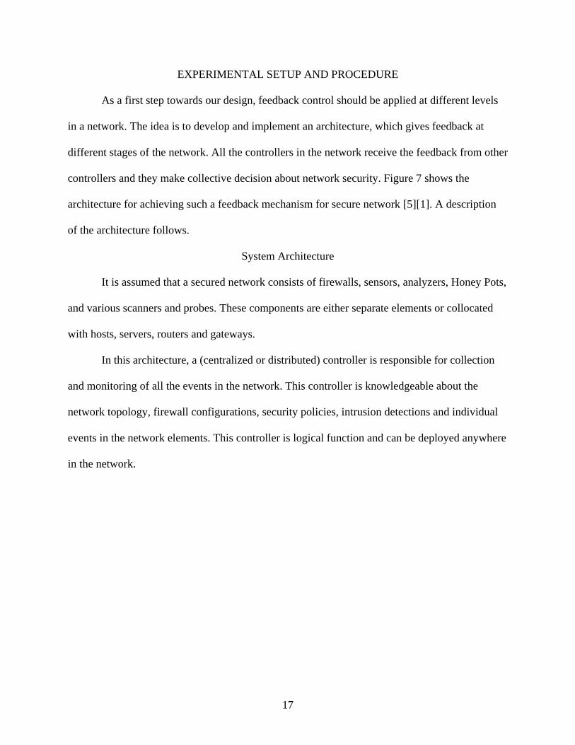
EXPERIMENTAL SETUP AND PROCEDURE
As a first step towards our design, feedback control should be applied at different levels
in a network. The idea is to develop and implement an architecture, which gives feedback at
different stages of the network. All the controllers in the network receive the feedback from other
controllers and they make collective decision about network security. Figure 7 shows the
architecture for achieving such a feedback mechanism for secure network [5][1]. A description
of the architecture follows.
System Architecture
It is assumed that a secured network consists of firewalls, sensors, analyzers, Honey Pots,
and various scanners and probes. These components are either separate elements or collocated
with hosts, servers, routers and gateways.
In this architecture, a (centralized or distributed) controller is responsible for collection
and monitoring of all the events in the network. This controller is knowledgeable about the
network topology, firewall configurations, security policies, intrusion detections and individual
events in the network elements. This controller is logical function and can be deployed anywhere
in the network.

18
Figure 7 Controller architecture for end-to-end security engineering.

19
Figure 7 shows the controller communicating with clients located in different network
elements. Clients are responsible for detection and collection of the events in the node and
communicate to the controller. Subsequently, controller will run through the algorithms, rules,
policies and mathematical formulas (transfer functions) for next course of action. These actions
are communicated to the clients.
As described in Figure 7, the architecture evolves from a concept of closed loop control.
Changes regarding the security behavior are captured and mixed with the incoming network
signals. This piece of information is used to formulate the next course of action. The final result
is an outcome from multiple loops and integration of multiple actions. The response times within
each loop are indicated in Figure 7. Response time varies from few milliseconds to several tens
of minutes. For example, nodal events like buffer overflows, performance degradation can be
detected in matter of milliseconds. On the other hand, it may take several seconds to detect
failed logins, changes to system privileges and improper file access.
The architecture explained above is for any network consisting firewalls, routers,
Intrusion Detection Systems etc. These are general elements used commonly in almost all
computer networks today. At different stages in the network different anomalies are detected and
decisions about required patches for the network are made. First step towards the development of
this architecture is to develop the first loop of the architecture explained which is the objective of
this thesis. At the first loop of the architecture nodal anomalies are detected. One of the
important anomalies detected on the infection of a system is; the system tries to make many
connections per second to spread the virus to as many systems as possible before any protection
against the virus can be applied. The model described below was developed to detect such an
anomaly, give the feedback and achieve control (reduce the rate of outgoing connections).

20
Model Description
Figure 8 shows the model at the nodal level. At this stage, the anomaly being observed is the
rate of outgoing connections. Connection requests block in Figure 8 represents any computer that
is connected to the network. As any other computer on the internet, it generates connection
requests. Connection requests generated are split into three categories.
• Connections to machines that are considered safe (a queue is maintained for safe list connections).
• Connections that are delayed (All the connection not present in the safe list but can go through).
• Connections that are dropped for other reasons (naturally).
Threshold
α
α
Suspect (Delay) queue
Safe Queue Connections requests
dβ
1- 2α
D
Connections not accepted
Figure 8 Model for connections accepted, delayed and rejected for parametric control.
If the system is not infected, then the system will make fewer outgoing connections per
second (less than 20 connections per second). All the connections generated should go out of the
system without delay. Therefore all the connections enter the safe queue and establish outside
connection. System makes more than 20 connections per second (set point) when infected. Set
point was chosen based on observing different worms explained in the previous section. Though
each worm has different value associated with it, average value is 20. This value can be tuned for
individual implemented. At this stage the controller should send signal to push more connections

21
to the delay queue to slow down the rate of outgoing connections. Connections after getting
processed by the delay queue are appended back to the safe queue and leave the system. Some
connections after staying in the delay queue for time specified by the user get dropped on
timeout. Timeout is application level timeout and not the protocol level timeout. Parameters
related to the size of the delay queue and the number of dropped connections is used to control
the total number of connections resulting in a slow down of spreading worm.
Sapphire worm spreading is taken as an example to show the applicability of this
approach. The goal of the example is to slow down the spreading velocity of a worm by
controlling the rate of connections (C(t)) detected by the host. A model capturing the behavior of
the system, i.e., how the number of total connections is changing is needed to achieve this goal
[6][7].
The rate of change of the number of connections (dc/dt) is proportional to the number of
dropped connections (-dc, where d is the specified drop rate) plus the number of connections
removed from the delayed queue (βD, where β is delay parameter and D is the number of
delayed connections on the queue) and the new successful connections (αu, where α is the
percentage of not delayed connections). This result in equation (3)
c dc D uβ α= − + +o
(3)
Differentiating Equation. 3 gives
[ ]c d c= −oo o
(4)
Substituting for co
gives
2c d c d D d uβ α= − + − +oo
(5)

22
The rate of change in the size of the delayed queue (dD/dt) is proportional to the new incoming
successful connections send to the queue (αu) minus the connections removed from the queue -
βd. This results in equation 6 below.
D D uβ α= − +o
(6)
Where D is the size of the delay queue; d is the drop rate; β is the delay parameter; u is the total
connections arriving; and α is the success rate
Combining equations for dC/dt and dD/dt in state variable format leads to Eqs. 7 and 8.
[ ]2
00
0 0
c cdc d d c d u
DD
β αβ αβ α
⎡ ⎤ ⎡ ⎤⎢ ⎥ −⎡ ⎤ ⎡ ⎤⎢ ⎥⎢ ⎥ ⎢ ⎥ ⎢ ⎥⎢ ⎥= − + −⎢ ⎥ ⎢ ⎥ ⎢ ⎥⎢ ⎥⎢ ⎥ ⎢ ⎥ ⎢ ⎥−⎣ ⎦ ⎣ ⎦⎢ ⎥⎢ ⎥ ⎣ ⎦⎣ ⎦
o
oo o
o
(7)
[ ]2
0 1 0 01 0 0 0
00 0 1 0
C cC
c ud d dC D
D
β α
⎡ ⎤ ⎡ ⎤ ⎡ ⎤⎡ ⎤⎢ ⎥ ⎢ ⎥ ⎢ ⎥⎢ ⎥⎢ ⎥ ⎢ ⎥ ⎢ ⎥⎢ ⎥= +⎢ ⎥ ⎢ ⎥ ⎢ ⎥− −⎢ ⎥⎢ ⎥ ⎢ ⎥ ⎢ ⎥⎢ ⎥⎢ ⎥ ⎣ ⎦⎣ ⎦ ⎣ ⎦⎢ ⎥⎣ ⎦
o
o
oo
(8)
Equations 7 and 8 represent state of output equations of the state model. Using these equations
the state model is simulated. Figure 9 shows the MATLAB® (MathWorks, Inc., Natick, MA)
simulation results of the state model.
As shown in the graph the system was tested to check the behavior by applying control at
different stages on spreading. Next stage after obtaining simulation results from MATLAB was
to implement the model in real computers, test the model and perform analysis on it. Below is

23
the description how the system was implemented using LabVIEW® (National Instrument
Corporation, Austin, Texas, www.ni.com).
Experimental Setup
Experimental setup consists of the first loop explained in the architecture of the previous
section. Any network consists of computers (hosts) at the bottom level. Bridges, switches,
firewall, Intrusion Detection Systems, routers etc form the higher layers of any computer
network. The objective of this thesis is to build and test the model at the host level (between two
computers). One important future works includes building similar controllers at different layers
of network and make them communicates with each other to make accurate decisions about the
network traffic patterns. The experimental setup of research consists of computers (hosts)
communicating with other computers using LabVIEW clients and server running UDP.
Implementing and testing the model require software which supports networking as well
as control system technology. LabVIEW 7.0 was found to be best suited for testing the model.
LabVIEW also has very useful tools for visual outputs. Data could be observed live and
modifications done online.
LabVIEW Model
LabVIEW user interface screen for the model is shown in Figure 9 below. It consists of
many numeric controls and indicators. It also has graphical interface to observe variations
graphically. The interface can be used to make connection to any system by changing the IP
address or a range of IP addresses can be given in a loop to make connection to many systems.
User can also set some other important parameters like timeout, delay for suspected queue, PID
gains and set point.

24
Figure 9 Front panel of LabVIEW client.

25
Connections are generated using LabVIEW’s graphical programming. Virus attack is
simulated mathematical equation for S-curve [3]. Disturbance is given to the system using
mathematical equation, simulating an attack. The user enters set point manually. Set point refers
to the number of connections per second any computer is allowed to make and is considered
safe. Acting by the mathematically simulated attack the computer increases its outgoing
connection rate. PID controller takes this as feedback and switches the connections between safe
and suspected queue (delay queue) to maintain a steady outgoing connection rate.
Timeout has been implemented at the application level. If the computer is infected and
makes very high rate of outgoing connections, then suspected queue builds up and many
connections timeout thereby avoiding many more infections. Below is description of some
important loops used in LabVIEW to implement the model.
Time to Synchronize Different Loops
Figure 10 Timer Loop for synchronous operation of all the loops.

26
The above block of the LabVIEW program shows the while loop which synchronizes
time between various blocks of the model. It runs at the speed of the processor. One of the clock
records the time at the start of the run and the other increments at the speed of the processor.
Difference between the two gives the time to synchronize all the loops.

27
Generation and Queuing
Figure 11 Simulation of attack and queuing.
The block shown above generates 5000 connections. This while loop uses UDP open connections to open ports from 60000 to
65000. The port number range was selected randomly to avoid conflicts with the already used ones. Random number block is used to
generate random numbers between 0 and 1. A numeric control is used to compare with the generated random

28
number and based on its output “safe” or “suspected” queue is selected. The program
implements a timeout independent of protocol timeout. To achieve this, the present time from the
clock loop is inserted into the queue along with the connections after converting both of them
into string data type as queue structure supports conversion of anything to string and back. The
connections are generated in S-shape to simulate an attack. The equation used to generate S-
function is given by
y = 200 - ((165*0.007)/((0.007+(165-0.007)*exp(-0.09*t)))+5);
The above mentioned exponential equation determines the delay between generating each
connection. Initially connections are generated at a rate of 5 connections per second, which is
considered safe. At the end of execution of the loop the number of connections per second will
increase to 33. LabVIEW takes 30 milliseconds to make a UDP connection. Therefore limitation
on the upper limit for the number of connections exists in LabVIEW.

29
Safe Connections
Figure 12 Makes outgoing connections from safe queue.
This loop makes connections, which are considered safe. At this stage in this research,
there is not enough intelligence in the system to decide which connections should be send to safe
queue and which ones should go to suspected queue. As mentioned before in the present
implementation random number or controller decides which queue the connections should go to.
Whatever connections go to safe queue are considered harmless and they need to be serviced
immediately without delay. This loop performs the required action and makes connections to the
client or server based on the IP address and port number specified as shown in the diagram. This
loop just de-queues the safe queue and makes the connection.

30
Delaying Suspected Connections
Figure 13 Delaying suspected connections and adding them back to safe queue; also dropping timed out connections.

31
Suspected connections are connections, which are considered harmful, which spreads
worm. These connections are sent to the suspected queue when queuing. These connections are
sent back to the safe queue after delaying, if they have not timed out. This loop processes
suspected queue at the specified rate. It separates the time string and connection string from the
element. Checks the time with the present time, if the difference is greater than the timeout
specified then drop the connection. If the connection is not timed out, the connection is pushed
into safe queue.
If the connection is timed out, then timed out connections should not be processes with
delay. Here the program logic resets the loop processing speed and timed out connections get
dropped without any delay.
PID Controller
Figure 14 Feedback loop with PID controller.
This loop performs feedback action using shift register. It shifts the old values of the
outgoing connection rate (dc/dt). PID gains (Kp, Ti and Td), set point and output range for the

32
controller can be modified. It gives output to the “ratio for each queue” (α). Ratio for each queue
determines the number of connections going to safe or suspected queue. As the number of
connections per second increases more than the set point controller increases/decreases the value
for “ratio for each queue” and sends more connections to the delay queue, thus reducing the
actual number of outgoing connections. Number of connections in the delay queue increases as
time progresses and also due to the slow processing speed of the delay loop.
At this stage in the research model for containment has been developed and tested real
time using LabVIEW. There are some differences in the MATLAB simulation of the model and
the LabVIEW implementation. Percentage values of the MATLAB model have been
implemented as time factors in LabVIEW. There fore the next step is to develop a relation
between them. This is done empirically. LabVIEW implementation is run many times and for the
time values set by the user, percentage of connections going to safe queue, suspected queue,
percentage of connections getting timed out and going back to safe queue from suspected queue
are calculated. To validate the system, values are used in Simulink® (MathWorks, Inc., Natick,
MA) model and validated. Simulink model is described below

33
Simulink Validation
Figure 15 Simulink model with a PID controller and the state variable model.
In Figure 15, the system represents the complete state space model. Constant (20)
represents the set point for the system (the maximum desired outgoing connections per second).
The PID controller controls the values for parameter α. A constant outgoing rate of 20
connections per seconds is achieved by the control system in Figure 15.

34
RESULTS AND DISCUSSIONS
First step in the implementation of this thesis is to implement the state model represented
by equations 7 and 8. Figures 16, 17, 18 and 19 shows the simulation result for feedback applied
to total number of connections, acceleration of outgoing connections and effect of applying to
different parts of the network.
Total Connections
Figure 16 Behavior of the state model for the control of the number of connections on the presence of a worm spreading according to an S-shape function. (a) Shows the total number of
connections with and without feedback.

35
The input in Eq. (8) represents the number of requested new connections per time unit. In
the case of a normal traffic the average number of requests can be considered constant over a
period of time. However, an S-shape form is expected for the spread function of a worm and
dU/dt=U (1-U) is used to generate the input. The solid line in Figure 16 represents the behavior
of the system with drop rate and delay parameters under “regular” conditions. The dashed lines
in Figure 16 represent the results for different detection times of the application of feedback
control for the scenario described above. As shown in the figure, control can be achieved at
different stages of attack and total number of connections being made still remains the same. As
expected, the sooner the infection is detected the faster the reduction of the spreading velocity.
Acceleration
Figure 17 Acceleration of outgoing connections for better detection times.
The acceleration of outgoing connections is used here as a detection mechanism to achieve
earlier detection because of second derivative. That is, when the acceleration reaches a certain
36
threshold the drop rate and the delayed parameters on the model in Equation (6) are adjusted to
slow down the spreading of the worm.
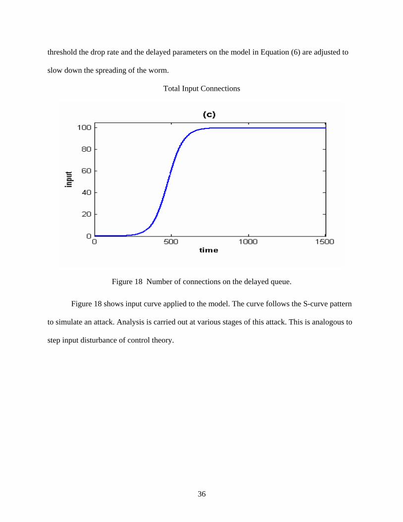
Total Input Connections
Figure 18 Number of connections on the delayed queue.
Figure 18 shows input curve applied to the model. The curve follows the S-curve pattern
to simulate an attack. Analysis is carried out at various stages of this attack. This is analogous to
step input disturbance of control theory.

37
Delay
Figure 19 Result of application of the feedback loop approach at the host and at the firewall
level.
Now, consider a scenario where hosts are connected to the firewall and a controller is
available at the hosts and at the firewall. The control can be done at the host level, at the firewall
level, or at both levels.
Figure 19 shows the results of applying or firewall converges to the same results though a
larger overshoot is observed at the firewall level. Regarding detection time, the acceleration at
the firewall level increases faster than at the host level and consequently an earlier detection time
is expected at the firewall level. As observed from
Figure 19, a double feedback loop has the advantage of the early detection time at the
firewall level and a more effective result in slowing down the infection.

38
LabVIEW Implementation
Next step after simulation of state model is to implement it in real time with feedback
PID controller. LabVIEW® (National Instrument Corporation, Austin, Texas, www.ni.com)
provides convenient toolsets to implement, test and observe the results.
After running the experiment more than twenty five times and finding the percentage of
connections going to each queue (α) and number of connections removed from suspected queue
and appended to safe queue was found to be
α = 0.5, β = 0.2 and Time out (θ) = 0.21
In the final model, outgoing rate of connections was taken for feedback and another
parameter timeout was introduced into the model. Therefore the model can be modified to
include timeout as shown in Figure 20 below
Safe QueueSafe Queue
Suspected Queue
Threshold β
θ
1-α
α
Delay queue
Accepted connections
D
Figure 20 State model implemented.

39
Important difference between the previous model is the introduction of timout. As can be
seen in equation (9) system matix A changes in the model implemented.
00 ( ) 1
C CN
DD
β αβ θ α
•
•
⎡ ⎤ ⎡ ⎤ ⎡ ⎤ ⎡ ⎤⎢ ⎥ = +⎢ ⎥ ⎢ ⎥ ⎢ ⎥⎢ ⎥ − + −⎣ ⎦ ⎣ ⎦ ⎣ ⎦⎣ ⎦
(9)
The final state model matrices were found to be
0 0.20 0.41
A⎡ ⎤
= ⎢ ⎥−⎣ ⎦
0.20.8
B⎡ ⎤
= ⎢ ⎥⎣ ⎦
[ ]0 0.2C =
[ ]0.2D =
So the state equations for the system are
0 0.2 0.20 0.41 0.8
C CN
DD
•
•
⎡ ⎤ ⎡ ⎤ ⎡ ⎤ ⎡ ⎤⎢ ⎥ = +⎢ ⎥ ⎢ ⎥ ⎢ ⎥⎢ ⎥ −⎣ ⎦ ⎣ ⎦ ⎣ ⎦⎣ ⎦
(10)
Where
N is the number of new connections
And the output equation is
[ ] [ ]0 0.2 0.2C C N• •⎡ ⎤ ⎡ ⎤= +⎢ ⎥ ⎢ ⎥⎣ ⎦ ⎣ ⎦
(11)
Transfer function of the system was found to be (sys = ss(a,b,c,d);)
x = tf(sys)
Transfer function:

40
0.2 0.2420.41
sTFs+
=+
(12)
Therefore, characteristics equation of the system is
S + 0.41 = 0 (13)
Finding poles of the system [y = eig(x)]
y = -0.4100
The system has a zero and a pole. The pole is located on the left side of y-axis. So the system is
stable.
Some of the experimental data appears in Figures 8 and 9. The red line in the plots shows
the rate of input connections to the system and the black line shows the outgoing rate. Where,
Ti is the reset time which is the inverse of reset rate, or how often the controller resets it output.
Td is the derivative time that defines the rate at which derivative action is taken.
Figure 21 Experimental result for Kp= 1, Ti = 0.01, Td = 0 & set point = 20, where time is in seconds and y-axis is number of connections per second.
The set point for the controller was set to 20. This means that no more than
approximately 20 connections should go through a host at any instant of time. Application and

41
protocol timeout is checked before en-queuing the delayed connections to the safe queue. In
Figure 21 a large overshoot and settling time is observed. This can be reduced by varying Ti
(Integration constant) as shown in Figure 22. The controller was set to Kp = 1.5, Ti = 0 & Td = 5
for the graph of the experiment below.
Figure 22 Experimental result for Kp = 1.5, Ti = 0 & Td = 5
Controllability & Observability
In state space model, one of the important concerns is whether we can steer the state via
the control input to certain locations in the state space. This property is called controllability or
reachability [10].
“The issue of controllability concerns whether a given initial state x0 can be steered to the
origin in finite time using input u(t)” [10].
If one can say something about the state of the system by observing the output, this
property is called observabiltity[10].
“Observability is concerned with the issue of what can be said about the state when one is
given measurements of the plant output” [10].

42
MATLAB® (MathWorks, Inc., Natick, MA) simulations showed that the system is
completely controllable. A rank of 3 was obtained. The system was also tested for observability
and rank of 3 was found.
Sample Results obtained for drop rate of five percent and delay of 1ms is shown below. The
controllability matrix is given by:
1.0000 0 -0.0500 0.0010 0.0025 -0.0001 -0.0500 0 0.0025 0.0005 -0.0001 0.0000 0 1.0000 0 -0.0010 0 0.0000
Observability matrix is given by:
0 1.0000 0 1.0000 0 0 0.0025 0 0.0005 0 0 1.0000 0.0025 0 0.0005 -0.0500 0 0.0010 -0.0001 0 0.0000 0 0 -0.0010 -0.0001 0 0.0000 0.0025 0 -0.0001 0.0000 0 -0.0000 0 0 0.0000
Rank for both controllability and observability were found to be 3. The results proves that the
system is both controllable as wells as observable.
Settling Time
Settling time is a very important parameter for the control system described above. It
signifies the time in which a worm can be controlled in our discussion. Figure 23 shows the
relation between settling time and period of integration. Smaller periods of integration are better
but it increases the steady state error as shown in Figure 24.
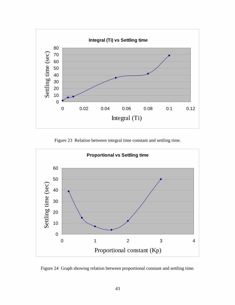
43
Integral (Ti) vs Settling time
01020304050607080
0 0.02 0.04 0.06 0.08 0.1 0.12
Integral (Ti)
Settl
ing
time
(sec
)
Figure 23 Relation between integral time constant and settling time.
Proportional vs Settling time
0
10
20
30
40
50
60
0 1 2 3 4
Proportional constant (Kp)
Settl
ing
time
(sec
)
Figure 24 Graph showing relation between proportional constant and settling time.

44
Figure 23 shows the relation between proportional constant and settling time. It can be
observed that the optimal value for the proportional gain is around 1.5. With the values obtained
from the analysis, controller can be tuned and containment can be achieved in very short span of
time.
Sensitivity Analysis
It is important to understand how changes in the parameters of the system affect its
results. For example, the effect of the delay parameter with respect to the steady state error and
the number of connections sent directly to the safe queue are of interest. The number of
connections sent directly to the safe queue is used here to exemplify the results of the analysis. A
simulation based sensitivity analysis, as shown in Eq. 14 is used to achieve these goals [18].
)()()(
xVxVxxVS
ρρ −+
= (14)
The value of V(x+ρx) represents the output of the system when parameter x is increased by a
certain value ρ. V(x) is the output of the system with no changes in the specified parameter.

45
Sensitivity Analysis
0246
81012
0 20 40 60 80 100 120
Delay
Sens
itivi
ty
Series1
Figure 25 Sensitivity of the number of connections sent directly to the safe queue as the delay parameter changes.
As seen in Figure 25, the sensitivity of the system with respect to the number of
connections that are directly sent to the save queue decreases as the value of the delay parameter
increases. It is expected that higher the value of the delay parameter, higher the number of
connections that will time out. If the delay is too large, all the connections in the delayed queue
will be eventually dropped. Therefore, as the delay increases the number of connections to be
sent to the safe queue converges to the set point (20 in this case). Consequently the sensitivity of
the referred parameter decreases as can be observed in Figure 25. This analysis is an indication
of the proper functioning of the system.
Limitations
This study is limited to communication between two computers. The experiment was
limited to two computers because at the node level any computer tries to communicate with
another machine one at a time and the scope can be extrapolated to bigger networks.

46
The implementation has been done using LabVIEW 7.0. LabVIEW is an excellent tool
for designing and analysis of such models where as its performance needs to be tested with
performance when same code is executed using other languages. Since time is such an important
issue in this study, it is a very important concern. Also LabVIEW can generate only 33
connections per second because it takes a minimum of 30 ms to generate each connection. The
model has been tested for set points of 10 or 20 connections per second.
The study is also limited by the protocol (UDP) used, the model and the system needs to
be tested for other protocols as TCP/IP. It also needs to take into consideration other anomalies
of virus attack such as CPU usage and memory overflow.
This research has been completely done on windows operating systems. Though other
operating systems such as UNIX, Linux and Java are also vulnerable, they have been built for
networking. Windows on the other hand is not built for networking from the onset.
Implementation, if done at the perimeter just by considering protocol connections then the kind
of operating system should not be a major concern [30].

47
CONCLUSIONS
In this research, a security architecture based on the feedback control theory has been
proposed. The first loop has been designed, developed and tested. The architecture proposes a
feedback model with many controllers located at different stages of network. The controller at
each stage gives feedback to the one at higher level and a decision about network security is
taken.
The first loop implemented in this thesis detects one important anomaly of virus attack,
rate of outgoing connection. Though there are other anomalies of a virus attack, rate of outgoing
connection is an important one to contain the spread. Based on the feedback model, this
symptom is fed back and a state model using queuing theory is developed to delay the
connections and slow down the rate of outgoing connections. Upon implementation of this
model, whenever an infected machine tries to make connections at a speed not considered safe,
the controller kicks in and sends those connections to a delay queue. Because of delaying
connections, rate of outgoing connections decrease. Also because of delaying, many connections
timeout and get dropped, reducing the spread.
PID controller has been implemented to decide the number of connections going to safe
or suspected queue. Multiple controllers can be implemented to control the parameters like delay
and timeout. Control theory analysis is performed on the system to test for stability,
controllability, observability. Sensitivity analysis is done to find out the sensitivity of the
controller to the delay parameter.
The first loop implemented gives feedback to the architecture proposed about symptoms
of an attack at the node level. A controller needs to be developed to receive information from
different controllers and decision about quarantining needs to be made. This research gives the

48
basic information needed for the controller about what is going on at individual nodes of the
network. This information can also be used to increase sensitivity of other loops to increase the
effectiveness of feedback architecture.
49
FUTURE WORK
LabVIEW® 7.0 (National Instrument Corporation, Austin, Texas, www.ni.com) has been
used as a tool to develop and test the model on Microsoft® Windows® operating systems
(www.microsoft.com). LabVIEW provides toolkits needed to develop and test the model. Visual
controllers and indicators provided by LabVIEW are suitable for developing and testing a model
because of the excellent user interface and real time monitoring capabilities, but they might
degrade the performance at the time of implementation. Alternative implementation technologies
needs to be explored and developed (for example developing the model in hardware or
implementing more efficient hardware oriented or less memory consuming software).
A major issue in the proposed model is how to identify if the new connection is a safe or
a suspect one. The solution depends on the domain knowledge and learning from the traffic
patterns. Also, currently there is limited number of hosts (i.e., 2) and it can be extended to large
number of hosts for large-scale analysis.
The model should be implemented at various stages of the network architecture. Each
controller should be able to interact with other controllers in the architecture and make decisions
based on the kind of traffic pattern. The whole architecture should be self-learning. Over a period
of time it should have a blacklist and white list patterns of the network traffic. This study has
been done on UDP traffic; future work would involve testing this architecture on different
networks and different protocols.
The entire architecture needs to be tested for false positives and performance. Delaying
traffic can be a major bottleneck in high-speed networks of today. Quarantining the infected
systems is one more area where more work can be done. Single system or part of a network can

50
be quarantined in case of infection. Architecture for performing such an action needs to be
developed.
To satisfy the feedback control loop, a specification and requirements for expected output
need to be specified. Also, certain measurements, benchmarks, and metrics are specified for
satisfying these requirements. Likewise, certain buffer size, CPU utilizations can also be
specified. Further work involves specification of requirements, and benchmarks, and deriving
transfer functions for each module in the feedback loop.
51
REFERENCES
1. Williamson, M.M, “Throttling viruses: Restricting propagation to defeat malicious mobile code.” Computer Security Applications Conference, December 2002. Proceedings. pp. 61 –68.
2. Lau, F.; Rubin, S.H.; Smith, M.H.; Trajkovic, L.; “Distributed denial of service attacks.” Systems, Man, and Cybernetics, 2000 IEEE International Conference, October 2000, vol. 3, pp. 2275 -2280
3. S. Staniford, V. Paxson, and N. Weaver. “How to own Internet in your spare time.” In Proceedings of the USENIX Security Symposium, August 2002, pp. 149-167.
4. David Moore, Vern Paxson, Stefan Savage, Colleen Shannon, Stuart Staniford, Nicholas Weaver, “The spread of the Sapphire worm.” Retrieved September 2004 from http://www.cs.berkeley.edu/~nweaver/sapphire/.
5. R.V. Dantu, “An architecture of security engineering.” ACSA Workshop on Application of Engineering Principles for Security System Design, November 2002.
6. R.V. Dantu “Feedback control for network security engineering.” 18th Annual ACSCA Conference on practical solutions to security engineering, December 2002.
7. João W. Cangussu, Ray A. DeCarlo, and Aditya P. Mathur, “A formal model of the software test process.” IEEE Transactions on Software Engineering, vol. 28, no. 8, pp. 782-796, August, 2002.
8. Somayaji, A., and Forrest, S., “Automated response using system-call-delays.”, Proceedings of the 9th USENIX security symposium, 2000.
9. João W. Cangussu, Ray A. DeCarlo, and Aditya P. Mathur, “Using sensitivity analysis to validate a state variable model of the software test process.” IEEE Transactions on Software Engineering, vol. 29, no. 5, pp. 782-796, May, 2003.
10. Graham C. Goodwin, Stefan F. Graebe and Mario S. Salgado, “Control system design.” Prentice Hall, 2001.
11. João W. Cangussu, Ray A. DeCarlo, and Aditya P. Mathur, “A state model for the software test process with automated parameter identification.” Proceeding of the 2001 IEEE systems, man, and cybernetics. Tucson, Arizona, pp. 706-711.
12. João W. Cangussu, Ray A. DeCarlo, and Aditya P. Mathur, “Feedback control of the software test process through measurements of software reliability.” Proceedings of the 12th IEEE international symposium on software reliability engineering, pp. 232-241, Hong Kong.
13. David Moore, Colleen Shannon, Geoffrey M. Voelker, Stefan Savage, “Internet quarantine: requirements for containing self-propagating code.” INFOCOM, 2003.

52
14. Feng-Li Lian, James Moyne, and Dawn Tilbury, “Network design consideration for distributed control systems.” IEEE transactions on control system technology, Vol. 10, No.2, March, 2002.
15. N. Gandhi, D.M. Tilbury, Y. Diao, J. Hellerstein and S. Parekh, “MIMO control of an apache Web server: modeling and controller design.” Proceedings of the American control conference, Anchorage, AK May 8-10, 2002.
16. N. Gandhi, D.M. Tilbury, J. Hellerstein and S. Parekh, “Feedback control of a Lotus notes server: modeling and control design.” Proceedings of the American control conference, Arlington, June 25-27, 2001.
17. David A. Nash, and Daniel J. Ragsdale, “Simulation of self-similarity in network utilization patterns as a precursor to automated testing of Intrusion Detection Systems.” IEEE transactions on systems, man, and cybernetics, Vol. 31, No. 4, July 2001.
18. Nong Yo, Xiangyang Li, Qing Chen, Syed Masum Emran and Mingming Xu, “Probabilistic techniques for intrusion detection based on computer audit data.” IEEE transactions on systems, man, and cybernetics, Vol. 31, No. 4, July 2001.
19. G.A. Fink, B.L. Chappell, T.G. Turner, and K.F. Donoghue, “A metric-based approach to Intrusion Detection Systems evaluation for distributed real-time systems.”
20. Richard A. Kemmerer and Giovanni Vigna, “Intrusion detection: A brief history and overview.” IEEE symposium on security and privacy, pages 27-30, 2002.
21. Joseph S. Sherif, Tommy G. Dearmond, “Intrusion detection: systems and models.” IEEE International workshops on enabling technologies: Infrastructure for collaborative enterprises (WETICE’02), 2002.
22. Christopher Kruegel, Fredrik Valeur, Giovanni Vigna, and Ricahrd Kemmerer, “Stateful intrusion detection for high-speed networks.” IEEE symposium on security and privacy, 2002.
23. Steven Bellovin, Jeffrey Schiller, “Security mechanisms for the internet.” IETF draft, draft-iab-secmech-01.txt, June 2002.
24. Dantu, R.; Cangussu, J.; Yelimeli, A.;”Dynamic control of worm propagation.” International conference on information technology: coding and computing, 2004. Proceedings. ITCC 2004. Volume: 1, April 5-7, 2004 Pages: 419 – 423.
25. Dantu, R.; Loper, K.; Kolan, P.;”Risk management using behavior based attack graphs.” International conference on information technology: coding and computing, 2004. Proceedings. ITCC 2004., Volume: 1, April 5-7, 2004 Pages: 445 – 449.
53
26. Andrea Saltelli, K. Chan, and E. M. Scott, “Sensitivity analysis.”, John Wiley & Sons, 2000.
27. Richard C. Dorf, Robert H. Bishop, Modern control systems, Ninth Edition, Prentice Hall –2001.
28. Wired, “Slammed! An inside view of the worm that crashed the internet in 15 minutes.” 2003, http://www.wired.com/wired/archive/11.07/slammer.html. (08/27/2004)
29. University of Michigan, control tutorials for MATLAB, “PID tutorial.” 1997, http://www.engin.umich.edu/group/ctm/PID/PID.html. (08/27/2004)
30. Paul Thurrott, “Windows uniquely vulnerable to viruses.” 1999, http://www.winnetmag.com/Article/ArticleID/18746/18746.html. (08/27/2004)
31. Symantec, “Norton Antivirus 2001 7.0 knowledge base.” 2004, http://service1.symantec.com/SUPPORT/nav.nsf/aab56492973adccd8825694500552355/024c927836400f528825675100593eb2?OpenDocument&src=sec_web_nam. (08/27/2004)