Computer modelling and geometric construction for four ...Computer modelling and geometric construction for four-point synthesis of 4R spherical linkages Kourosh H. Shirazi * Department

Applied Mathematical Modelling 31 (2007) 1874–1888

www.elsevier.com/locate/apm

Computer modelling and geometric constructionfor four-point synthesis of 4R spherical linkages

Kourosh H. Shirazi *

Department of Mechanical Engineering, Faculty of Engineering, Chamran University of Ahvaz, Ahvaz, Iran

Received 1 May 2005; received in revised form 1 May 2006; accepted 27 June 2006Available online 28 August 2006

Abstract

In this paper, computer modelling and geometric construction of Burmester curve for synthesis of spherical mechanismsis presented. Rigid shell guidance in four specified positions on a sphere is performed by a 4R spherical linkage. The syn-thesis of such a linkage requires obtaining the associated Burmester curves on the reference sphere. Based on the Burmestertheory and beside the computational and modelling abilities of the symbolic mathematical software namely Maple, anaccurate as well as fast procedure for geometric construction of Burmester curve is developed. In the first part, the conceptsof orientation and position on the sphere, pole of the motion and the related parameters are extended for modelling by theMaple. In the second part, the concepts of complementary axis quadrilateral and its imaginary motion, the center and cir-cle axis cones and Burmester curve are derived. In the final part, using the prepared procedure and through a numericalexample, a 4R spherical linkage for guiding an antenna to meet four specified postures in a three-dimensional workingspace is synthesized.� 2006 Elsevier Inc. All rights reserved.

Keywords: Rigid body guidance; Complementary axis quadrilateral; Burmester curve; Four-point synthesis; Spherical mechanism; Maple;Space antenna

1. Introduction

Beside the spatial mechanisms, the spherical linkages can be employed for doing the complex mechanicaltasks e.g., rigid body guidance and function generation in three-dimensional work spaces. The kinematic andgeometric properties of the spherical linkages can be intuitively understood by an analogy between the motionon a sphere and motion on a plane. In the spherical linkages every link rotates about the same fixed points.Thus, trajectories of points in each link lie on concentric sphere with this point as the center or referencesphere. Only the revolute joint (R-type joint) is compatible with this rotational movement and its axis mustpass through the fixed point which is the center point of the reference sphere. So, one of the simplest possibleclosed chain configurations is 4R linkage. In our problem coupler of a 4R linkage should meets four specified

0307-904X/$ - see front matter � 2006 Elsevier Inc. All rights reserved.

doi:10.1016/j.apm.2006.06.013

* Tel.: +98 6113 360428; fax: +98 6113 337010.E-mail address: [email protected]

mailto:[email protected]

K.H. Shirazi / Applied Mathematical Modelling 31 (2007) 1874–1888 1875

positions on the same sphere. This problem has been considered before [1,2]. Several approaches have beenproposed with the aim of finding the solution of this problem, including algebraic methods, complex numbers,CAD based method and matrix methods [3–7]. The first spherical mechanism computer-aided design programwas written by Larochelle et al. [4] also Ruth and McCarthy [5] used the fundamental Burmester geometricalsynthesis theory for describing a computer-aided design system namely SPHINX package for synthesis ofspherical four-bar linkages. Al-Widyan and Angeles [6] described the analytical description of the motionon the sphere for synthesis of spherical mechanism. They assigned that the analytical description of the motionis not as simple as geometrical one. The analytical based method for five points of accuracy synthesis of 4Rspherical linkages has been studied by Alizade and Kilit [7]. Also McCarthy [8] described the analytical andgraphical aspects of planar, spherical and spatial synthesis of linkages. In spite of simplicity of the graphicaland the geometrical understanding of motion on the sphere, the implementation of the geometrical construc-tion always accompanies the associated complexities and lack of accuracy. Modelling of the problem by themicrocomputers can be a possible method to overcome the geometrical and computational complexities. Butemployed computer software should possess abilities of both geometrical and computational modelling. TheMaple software among the symbolic mathematical software has both the capabilities. The abilities of this soft-ware in synthesis of planar 4R linkages with four points of accuracy have been explained by Shirazi [9]. In thiswork, the geometric tools of this software are employed to explain and analyze the kinematic concepts of rigidbody motion such as transformation and rotation of objects in three-dimensional workspaces. Thus conceptsof poles of motion, complementary axis quadrilateral and the center-circle point and Burmester curves in thespherical geometry and . . .are modeled and developed. Using the prepared procedure a sample numericalproblem in the category of motion generation for four specified postures on the sphere is solved. The illus-trated problem is synthesis of a mechanism for the accurate positioning of an antenna dipole of a radio tele-scope. The simplicity aroused by the modelling and solution procedure can open new horizons for applicationof spherical linkages.

2. Position and attitude of a shell on the sphere

The problem is defined as design of a spherical 4R linkage that its coupler which is a spherical shell meetsfour specified positions. To model the problem the position of the coupler shell should be defined. Fig. 1depicts spherical arc AB and the reference sphere centered at point Q with radius equal to unity. To definethe shape, position and orientation of AB four angles a, b, q and f are used. The position of point A is definedwith azimuth-elevation set of angles namely q and f. The shape of the arc AB is defined by angle a. It should benoted that the arc AB is a geodesic arc (grate circle of the sphere). The orientation of the arc AB is defined by

Fig. 1. Definition of position and attitude of spherical arc AB.

Fig. 2. Geometric configuration of the geodesic arc AB.

1876 K.H. Shirazi / Applied Mathematical Modelling 31 (2007) 1874–1888

meridional angle b. This definition of a geodesic arc on the unity sphere can be used for a spherical shell in thesame manner. In other words, definition of the position and orientation of a spherical shell can be accom-plished by position and orientation of a specified geodesic arc belonging to the shell.

A Maple program has been prepared to accomplish all stages of the modelling and construction. The Maplecodes are mentioned in Appendix I. Beside the description of the modelling and construction procedure, theassociated Maple codes are indicated and explained. Suppose the posture of geodesic arc AB should be definedon the reference sphere (which is posture of any shell contains AB). In the beginning of the program the mem-ory is refreshed using the command ‘restart’ (line 1). The related packages for performing the program areopened using the command ‘with’ (lines 2–4).

The origin of the coordinate system namely point Q and the reference sphere namely RS, are defined usingthe commands ‘point’ and ‘sphere’, respectively (lines 5 and 6). Through the lines 7–8 a procedure for defini-tion of the first point of any spherical arc using the azimuth-elevation coordinates is provided, the angles q andf are denoted by ‘_theta’ and ‘_phi’, respectively. Through the lines 8–9 a procedure is provided for obtainingthe end point of any spherical arc starting at point ‘_FirstPoint’, with the arc shape angle a equal to ‘_Arc-Angle’ and the meridional angle b equal to ‘_MeridionalAngle’. In this procedure which is named as ‘Final_point()’ as depicted in Fig. 2 the vector ~QA rotates about vector k � ~QA through angle a then the new vector~QA0 rotates about ~QA through angle b and therefore the final point of the arc namely point B is obtained. In

the procedure ‘Final_point()’, the command ‘crossprod(Z_axis,_QA)’ provides the cross product of two vec-tors ‘Z_axis’ and ‘_QA’, command ‘rotation’ rotates the considered object ‘_SecondPoint’ about the rotationaxis ‘L_QA’ through the desired angle ‘_MeridionalAngle’. In lines 9–10 a procedure namely ‘Arc(E,F)’ is pre-pared to draw a geodesic arc between two arbitrary points ‘E’ and ‘F’ on the same sphere. In lines 10–13 usingthe defined procedures four postures of arc AB are defined and displayed.

3. Central axis and pole

Let consider Fig. 3. In this figure spherical shell ABC is shown in its two successive positions. The cen-tral axis of motion of the shell is a hypothetical axis namely Q–Q for rotation of the shell from its initialposition A1B1C1 to the final position A2B2C2. In the planar motion the pole is defined rather than thecentral axis. Comparing two postures of the shell ABC, it is seen that two positions of each point of the shellare in the same distance of the central axis. It may lead us to find a method for construction of the centralaxis.

Fig. 3. Central axis and pole of spherical motion of shell ABC.


Lemma. Suppose plane PA and PB (Fig. 3) denote the loci of all points with the same distance to the points A1,

A2 and B1, B2, respectively. The intersection of these two planes (line Q–Q), is the central axis of shell ABC in

rotation from the initial state A1B1C1 to the final state A2B2C2.

Proof. Let assume the spherical triangle (or the considered shell) ABC has been fixed to the reference sphere,also assume the reference sphere have enough mobility to rotate about its center. The axis of rotation of thesphere from its initial state that triangle ABC is in the A1B1C1 position to its final position that triangle ABC isin the A2B2C2 position, is the central axis of the sphere and the triangle ABC. Now let the central axis beanother line as L–L, instead of Q–Q. Since the sphere rotates about the L–L, all of sphere’s points rotate aboutL–L so the distance of every point on the sphere to the line L–L before and after rotation are the same. Thismeans that we have

A1H A ¼ A2H A; B1HB ¼ B2H B and C1H C ¼ C2H C;

where HA, HB and HC are projection points of A, B and C, respectively. Because HA on the line L–L, belongsto plane PA also O belongs to both L–L and PA the line L–L is coincided with plane PA. By the same reason itone can say that line L–L belongs to plane PB and PC, too. Therefore line L–L lies on the intersection ofplanes PA, PB and PC. This means that L–L is the line Q–Q. h

Now let consider points of intersection of the line Q–Q and the sphere, using the geometry on the sphere,the motion of shell ABC can be expressed in another way. In Fig. 3 two points namely P12, are called pole ofmotion of the shell ABC in the spherical geometry.

The geometric construction for obtaining the central axis and poles of motion of a shell can be simply doneby a few commands in Maple. Through lines 14–15 a procedure namely ‘Ce_Ax()’ is prepared to obtain thecentral axis as well as poles of the motion of an object with initial posture defining by its two points ‘_A1’ and‘_B1’ to the final posture defining with two point ‘_A2’ and ‘_B2’. The final result for central axis and pole aredenoted by names ‘_CentralAxes’ and ‘_Pole’, respectively.

In this procedure using command ‘dsegment’ two vectors ‘_A12’ and ‘_B12’ are defined such that the for-mer starts from ‘_A1’ and ends in ‘_A2’ and the latter starts from ‘_B1’ and ends in ‘_B2’. Then the plane PA

and PB (Fig. 3) are defined using command ‘plane’ and are denoted by ‘PlaneA’ and ‘PlaneB’. By command‘plane’ two planes ‘PlaneA’ and ‘PlaneB’ are defined by one point such as ‘Q’ in the planes and the normalvector at the plane which are the vectors ‘_A12’ and ‘_B12’, respectively. Command ‘intersection’ finds theintersection line of the two planes and is denoted by the name ‘_CentralAxis’. One more time using command‘intersection’ the pole is found with intersecting the central axis ‘_CentralAxis’ with the reference sphere ‘RS’and is denoted by name ‘_Pole’.


4. Four successive postures and complementary axis quadrilateral

Now four specified postures of a shell are considered. For each two positions one central axis can bedefined. Thus, six central axes are obtained. Through lines 15–16 six poles P12, P13, P14, P23, P24 and P34

and the associated central axes are found through two ‘for do’ loops. The ith and ith poles and central axesare denoted by the names ‘Polekikj’ and ‘Cpkikj’, respectively. Using symbol ‘ki’ after a parameter in Maple,points to the ith element of that parameter.

In our problem we are looking for a 4R linkage which is capable to move the coupler shell such that meetsfour specified postures defined on the reference sphere. The linkage possesses two fixed and two moving jointsall laying on the reference sphere. A moving joint is the point of the coupler shell that when the coupler meetsfour specified positions it places on the equal distance of a fixed joint.

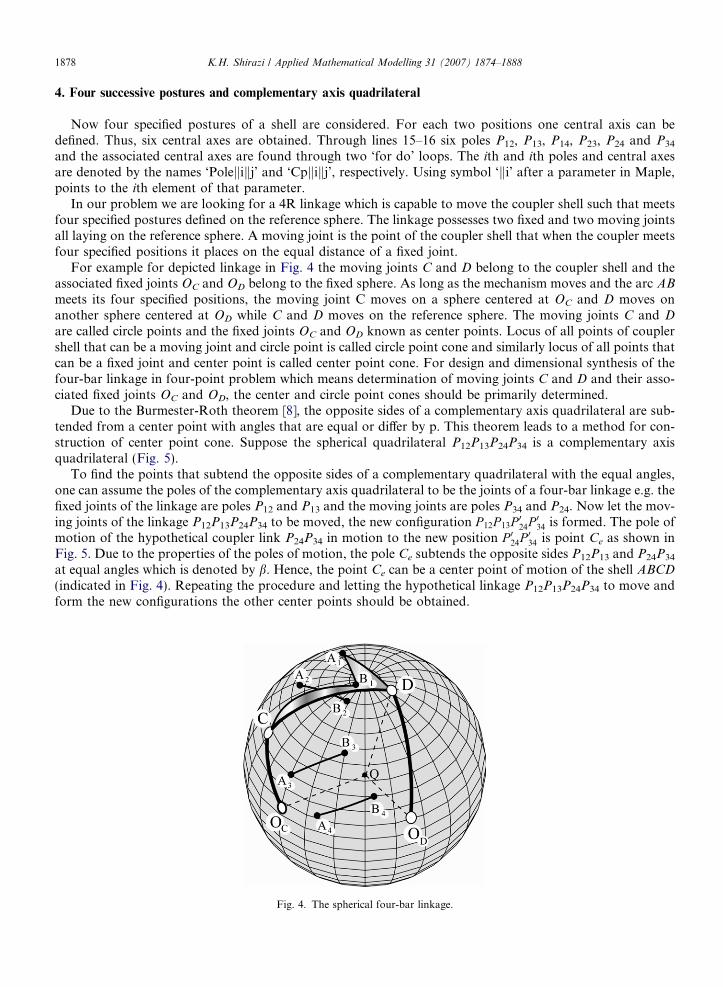
For example for depicted linkage in Fig. 4 the moving joints C and D belong to the coupler shell and theassociated fixed joints OC and OD belong to the fixed sphere. As long as the mechanism moves and the arc AB

meets its four specified positions, the moving joint C moves on a sphere centered at OC and D moves onanother sphere centered at OD while C and D moves on the reference sphere. The moving joints C and D

are called circle points and the fixed joints OC and OD known as center points. Locus of all points of couplershell that can be a moving joint and circle point is called circle point cone and similarly locus of all points thatcan be a fixed joint and center point is called center point cone. For design and dimensional synthesis of thefour-bar linkage in four-point problem which means determination of moving joints C and D and their asso-ciated fixed joints OC and OD, the center and circle point cones should be primarily determined.

Due to the Burmester-Roth theorem [8], the opposite sides of a complementary axis quadrilateral are sub-tended from a center point with angles that are equal or differ by p. This theorem leads to a method for con-struction of center point cone. Suppose the spherical quadrilateral P12P13P24P34 is a complementary axisquadrilateral (Fig. 5).

To find the points that subtend the opposite sides of a complementary quadrilateral with the equal angles,one can assume the poles of the complementary axis quadrilateral to be the joints of a four-bar linkage e.g. thefixed joints of the linkage are poles P12 and P13 and the moving joints are poles P34 and P24. Now let the mov-ing joints of the linkage P12P13P24P34 to be moved, the new configuration P 12P 13P 024P 034 is formed. The pole ofmotion of the hypothetical coupler link P24P34 in motion to the new position P 024P 034 is point Ce as shown inFig. 5. Due to the properties of the poles of motion, the pole Ce subtends the opposite sides P12P13 and P24P34

at equal angles which is denoted by b. Hence, the point Ce can be a center point of motion of the shell ABCD

(indicated in Fig. 4). Repeating the procedure and letting the hypothetical linkage P12P13P24P34 to move andform the new configurations the other center points should be obtained.

Fig. 4. The spherical four-bar linkage.

Fig. 5. Complementary axis quadrilateral and obtaining center point Ce.


Using the same construction the circle points can be obtained. The main difference in generating the circlepoints is in the selection of the complementary axis quadrilateral. A circle point is a point that subtends theopposite sides of a image quadrilateral. This quadrilateral consists of four vertexes including the image polesof motion. Suppose the shell is assumed as the fixed body and let the reference sphere to rotate about the ori-gin Q. In this case six poles can be found for the motion of the sphere with respect to the first position of theshell. These poles are called the image poles and the associated axes of rotation are called the image centralaxes [1]. The image poles are named by P 1

23, P 124, P 1

34, P12, P13 and P14. It should be noted that since the shell isfixed in the 1st position the poles and image poles with subscript 1 are placed in the same place. However theimage poles without subscript 1 as pole P 1

nm can be obtained by reflecting the pole Pnm relative to the planepassing through three points P1n, P1m and Q.

Referring to the Maple program in Appendix I, through line 16 all required planes to define the image polesare defined using command ‘plane’. The names of the planes are selected such that remind the three includingpoints, for example name ‘Plane_QP12P13’ means the plane passing through three points Q, P12 and P13. Nowusing command ‘reflection’ all the required image poles are obtained through the line 17. Command ‘reflec-tion(P24_1, P24, Plane_QP12P14)’, reflects the point ‘P24’ with respect to the plane ‘Plane_QP12P14’ andis denoted by ‘P24_1’. Now to form the image quadrilateral through line 18 two fixed joints ‘FixedJoint_A’and ‘FixedJoint_B’ are selected laying on poles P12 and P13, respectively. The two moving joints ‘Moving-Joint_E0’ and ‘MovingJoint_F0’ are selected laying on image poles ‘P34_1’ and ‘P24_1’, respectively. Throughlines 20 and 21 two spheres are define one centered at fixed joint A and radius AF0 and the other centered atfixed joint B and with radius BE0. For better imagination consider Fig. 6.

After selection of image quadrilateral P 12P 13P 124P 1

34, let the hypothetical four-bar moves to achieve new con-figuration P 12P 13P 10

24P 1034. Then as it was previously explained, the pole of motion of link P 1

24P 134 which is shown

as Ci is the circle point. The procedure showing in Fig. 6 can be implemented by Maple commands. Lines21–29 contains a ‘for do’ loop to automatic generation of circle points. The input link AF0 rotates about A

through angle b. Command ‘rotation’ in line 22 finds the new position of point F0 (Fig. 6) and is denotedby ‘MovingJoint_Fki’. To find the new place of moving joint E0 (Fig. 6) through the lines 23 and 24 usingthe command ‘solve’ the intersection of the three spheres including the reference spheres ‘RS’, the sphere‘Sphere_Fki’ (centered at ‘MovingJoint_Fki’ with the radius equal to distance of two points ‘MovingJoint_F0’and ‘MovingJoint_E0’) and ‘Sphere_B’ (centered at ‘FixedJoint_B’ with the radius equal to distance of twopoints ‘FixedJoint_B’ to ‘MovinJoint_E0’) is found. The three spheres are intersecting in two points whichboth are circle points. In Fig. 6 one of these two points is shown as point P 10

24. Using the old and new config-urations the circle point is found. This is done through line 26 and for the other solution the circle point isobtained through line 28. Repeating the loop, all the circle points are obtained. To obtain more circle

Fig. 6. Image quadrilateral and obtaining circle point Ci.


points and as a result a smoother locus, increments of angle b (in line 21) should be assumed as the smallervalues.

Although according to the above mentioned descriptions the circle and center point curves can be derivedseparately using the associated opposite quadrilaterals, since for each circle point there is just one central axisand two center points it is prefer to obtain the circle point curve then finding the associated center point foreach circle point. This method not only makes the derivation of center point curve to be simpler, it is moreefficient during the design and synthesis.

5. The corresponding center point for a circle point

To describe the method of determination of center point associated to a specified circle point let considerFig. 7. As is indicated in this figure the associated center point (OC) of the circle point C1 is considered to befound. The point OC is center point of point C1 when this point is placed on its four positions C1, C2, C3 andC4 during its motion. So if the four positions of the point C1 are found, the intersection of three perpendicularbisector planes of C1–C2, C1–C3 and C1–C4 would be the point OC. Using the procedure similar to the planarcase [9] to obtain point C2 first reflecting point C1 with respect to the plane PQP 12P 13

which is passing through

Fig. 7. The cardinal points and center point associated to the circle point C1.

Fig. 8. The center and the circle points.


three points Q, P12 and P13, the cardinal point associated to the point C1 and related to the spherical triangleP12P13P23 can be found. This point is denoted by L123.

Now reflecting the cardinal point L123 with respect to the planes PQP 12P 23and PQP 13P 23

, C2 and C3 are found,respectively. Using the same procedure after determination of cardinal point L124 (which is derived by reflec-tion of point C1 with respect to the plane PQP 12P 14

Þ point C4 can be found with reflection of cardinal point L124

with respect to the plane PQP 14P 24.

The Maple procedure for determining the center points associated to each circle point C1 is presentedthrough the lines 30–38. In line 30 a procedure which is named ‘Cen_Four’ is defined by which the center pointof four specified points such as ‘Mov-Pin1’, ‘Mov-Pin2’, ‘Mov-Pin3’and ‘Mov-Pin4’ can be found. The derivedcenter point is denoted by ‘Fix-Pin1’. As it was explained the essence of deriving procedure is based on thedetermination of intersection points of the three perpendicular bisector planes. These planes are defined usingtheir normal vectors ‘dm12’, ‘dm13’ and ‘dm14’ and one point belonging to the plane as point ‘Q’. The planesare denoted by local variables ‘pm12’, ‘pm13’ and ‘pm14’. Using a ‘for do’ loop starting at line 31 and endingat line 38 all the corresponding center points of the circle points are found. In lines 32 and 33 the cardinalpoints of the considered circle point with respect to the spherical triangles P12P13P23 and P12P14P24 whichare denoted by ‘Cardinal_point_123’ and ‘Cardinal_point_124’, respectively are found. Through the lines34–37 three positions associated to the point ‘Position_C1ki’ are found and denoted by ‘Position_C2ki’,‘Position_C3ki’ and ‘Position_C4ki’ respectively. Fig. 8 shows the plot of center and the circle points.

To display the results on the same sphere, two commands ‘draw’ and ‘display’ are used via lines 39–41.It should be noted that despite the obtained solutions mathematically satisfy the condition of generation of

four specified postures by the desired linkage, in some cases the solution due to the branching problem, thecoupler cannot meet the four postures smoothly and successively by continuous motion of the linkage. Thisproblem can be suppressed by rectification of solution. The rectification of solution for function generationsynthesis of planar linkages has been considered by Filemon [10] and Waldron [11] and has been generalizedfor spherical linkages by McCarthy [8]. Since the problem here is synthesis of motion generation instead offunction generation, to be sure that the selected linkage generates a rectified solution, one can simply animatethe linkage by a three-dimensional modelling software such as ADAMS VIEW, VISUAL NASTRAN orCOSMOS MOTION after selecting a possible solution among all solutions.

6. Design of platform for a space radio-telescope antenna

To show the capabilities of the Maple program in design of the 4R spherical mechanisms, let consider theproblem of design of platform for a space radio-telescope antenna. The antenna should be able to trackthe emitted radio signals from a specified star. Due to the rotational motion of the earth the orientation ofthe polarization plane of the receiving signals are continuously changed therefore, the antenna collector dipole

Fig. 9. Space radio-telescope antenna in the four specified positions.

Table 1The information of the dipole position and orientation during the motion

i hi (deg) /i (deg) bi (deg)

1 90 65 52 70 40 163 40 20 254 10 15 40


(A 0B 0 in Fig. 9) during the tracking should be oriented and rotated to be coincided with the polarization planeof the receiving signals. The schematic figure of the system is depicted in Fig. 9. We decided to employ a 4Rspherical mechanism to move support of the antenna to the specified proper positions as well as orientations.

The platform is the coupler shell of the linkage. To solve the problem the fixed and moving joints of thelinkage should be found. The corresponding values to the four specified positions and orientation of the dipolehave been defined by the cosmological information. The typical values for position and orientation are men-tioned in Table 1.

The arc length is assumed to be a = 30�. Using the above values and the program in Appendix I the centerand circle point curves are obtained. The center and circle point curves and four specified postures of an asso-ciated arc to the dipole AB on the reference sphere (arc AB) are shown in Fig. 10. After deriving the circle andcenter point curves to select the fixed and moving joints of the linkage two points of the center point curve areselected to be the fixed joints OC and OD. From the mathematical point of view all the solutions derived as thecenter point can be used as the mechanism’s fixed joint. But in the engineering applications it should be notedthat the designer could examine that how the selected mechanism performs the defined task. The range ofrocking motion of the input and output links and also motion of the coupler of the mechanism based onthe specified sequence can be some criteria that the designer may be considered to select the better set of fixedor moving joints. The associated circle points C and D are obtained easily, e.g. if the fixed joint OC is selectedas ‘Center_pointkJ1’ the associated moving joint namely C simply would be ‘Circle_pointkJ1’ and vice versa.The designed linkage is depicted in Fig. 11. It is seen that the mechanism can place its coupler shell ABCD suchthat the arc AB meets the four specified postures.

Fig. 10. The circle and the center point curves and four postures of AB.

Fig. 11. The solution mechanism places AB in the four specified postures.


7. Concluding remarks

In the present work the geometrical procedure of four-point synthesis of the spherical linkages wasdescribed. Using the geometrical capabilities of the symbolic mathematical software namely Maple, the


procedure is implemented by computer. This program not only directly uses the geometrical concepts as rota-tion, reflection, plane and direct segments it uses the benefits of accurate and fast computation of thecomputers.

The program according to the four specified positions of a shell finds the corresponding complementaryaxis quadrilateral. Then constructing the equivalent four-bar linkage which coincided with on the complemen-tary axis quadrilateral and determining the various configuration of the linkage, all circle points are found.The center points are obtained using the circle points and the associated cardinal points. Selecting two centerpoints as the fixed joints and finding the associated circle points as the moving joints the desired four-bar link-age is designed. It should be noted that since the circle and center point curves are obtained, the designer dueto the fitness of the solution with the practical limitations can select the best linkage among all the availablesolutions. These limitations can be available working space, range of rocking motion of the input and the out-put links and avoiding the branching problem. To show the capabilities of the program in design of the 4Rspherical linkages a spherical mechanism for positioning the antenna dipole of a radio telescope is designed.

Appendix I

> # Refresh the memory.line1: restart:

> # Opening the standard packages.line2: with(geom3d,line,rotation,sphere,point,dsegment,xcoord,ycoord,

zcoord,draw,midpoint,plane,intersection,Equation,detail,

coordinates,distance,rotation,reflection,center,radius,

FindAngle,AreCoplanar):

line3: with(linalg,vector,matrix,crossprod,angle):

line4: with(plots,display,spacecurve,implicitplot3d,pointplot3d):

> # Definition of the reference sphere.line5: point(Q,[0,0,0]):

line6: sphere(RS,[Q,1.]):

> # Procedure of definition of position of a point on the shell.line7: Initial_point:¼proc(dtheta,dphi)::point;

local _SphPoi,theta,phi;theta:¼evalf(Pi/180.*dtheta):phi:¼evalf(Pi/180.*dphi):point(_SphPoi,[cos(phi)*cos(theta),cos(phi)*sin(theta), sin(phi)]);end proc:

> # Procedure of definition of position of another point.> line8: Final_point:¼proc(_FirstPoint,_ArcAngle,_MeridionalAngle)::point;

local _Final,_SecondPoint,_Normal,L_QA,Z_axis,_QA;global Q;

_QA:¼[xcoord(_FirstPoint),ycoord(_FirstPoint),zcoord(_FirstPoint)]:Z_axis:¼[0,0,1]:_Normal:¼crossprod(Z_axis,_QA):line(L_Normal,[Q,_Normal]);rotation(_SecondPoint,_FirstPoint,evalf(_ArcAngle*Pi/180.),L_Normal);line(L_QA,[Q,_QA]):rotation(_Final,_SecondPoint,evalf(_MeridionalAngle*Pi/180.),L_QA):end proc:

> # Procedure of drawing of a geodesic arc between points E and F.line9: Arc:¼proc(E,F)::list;

local nEF,vE,vF,LEF,aEF,poa,ii,M;

global Q;

vE:¼[xcoord(E),ycoord(E),zcoord(E)]:


vF:¼[xcoord(F),ycoord(F),zcoord(F)]:nEF:¼crossprod(vE,vF):line(LEF,[Q,nEF]):

aEF:¼angle(vE,vF):M:¼5:for ii from 0 to M do

rotation(poakii,E,aEF*ii/M,LEF):od:

spacecurve([seq([xcoord(poakjj),ycoord(poakjj),zcoord(poakjj)], jj=0� � �M)],style=LINE,color=BLACK);

end proc:

> # Definition of four positions of point A.line10: A1:¼Initial_point(0,85.):

A2:¼Initial_point(10.,75.):A3:¼Initial_point(30.,50.):A4:¼Initial_point(50,30.):

> # Definition of four positions of point B.line11: B1:¼Final_point(A1,30.,�120.):

B2:¼Final_point(A2,30.,�90.):B3:¼Final_point(A3,30.,�60.):B4:¼Final_point(A4,30.,�70.):

> # Drawing four arc AB in its four positions and the sphere.line12: Draw_arc1:¼Arc(A1,B1):

Draw_arc2:¼Arc(A2,B2):Draw_arc3:¼Arc(A3,B3):Draw_arc4:¼Arc(A4,B4):Draw_sphere:¼draw(RS,color=gray,style=WIREFRAME):Draw_point:¼draw([A1,A2,A3,A4,B1,B2,B3,B4],view=[�1.2� � �1.2,

�1.2� � �1.2,�1.2� � �1.2], symbol=circle,color=black):> # Display of the drawings.line13: display({Draw_point,Draw_sphere,seq(Draw_arcki,i=1� � �4)}, color=black);

> # Procedure for finding the central axis and pole.Line14: Ce_Ax:¼proc(_CetralAxis,_Pole,_A1,_A2,_B1,_B2)

global Q,RS;

local _A12,_B12,_PlaneA,_PlaneB,_Poles;


unassign(_Poles);dsegment(_A12,[_A1,_A2]):dsegment(_B12,[_B1,_B2]):plane(_PlaneA,[Q,_A12]):plane(_PlaneB,[Q,_B12]):intersection(_CetralAxis,_PlaneA,_PlaneB):intersection(_Poles,_CetralAxis,RS):if evalf(zcoord(_Poles[1])) > 0

then point(_Pole,coordinates(_Poles[1]));else point(_Pole,coordinates(_Poles[2]));fi;

end proc:

> # Obtaining the six poles related to the four postures.Line15: for i from 1 to 3 do

for j from i + 1 to 4 do

Ce_Ax(CPkikj,Polekikj,Aki,Akj, Bki,Bkj):od:

od:

> # Definition of the necessary plane to obtain image poles.line16: plane(Plane_QP12P13, [Q, Pole12, Pole13]):

plane(Plane_QP12P14, [Q, Pole12, Pole14]):plane(Plane_QP12P23, [Q, Pole12, Pole23]):plane(Plane_QP12P24, [Q, Pole12, Pole24]):plane(Plane_QP13P23, [Q, Pole13, Pole23]):plane(Plane_QP13P14, [Q, Pole13, Pole14]):plane(Plane_QP14P24, [Q, Pole14, Pole24]):plane(Plane_QP23P34, [Q, Pole23, Pole34]):plane(Plane_QP24P34, [Q, Pole24, Pole34]):plane(Plane_QP13P34, [Q, Pole13, Pole34]):

> # Obtaining the image poles.line17: reflection(Pole24_1, Pole24, Plane_QP12P14):

reflection(Pole34_1, Pole34, Plane_QP13P14):> # Definition of image quadrilateral.line18: FixedJoint_A :¼Pole12:

FixedJoint_B :¼Pole13:MovingJoint_E0:¼Pole34_1:MovingJoint_F0:¼Pole24_1:

> # Definition of the necessary lines to move the image quadrilateral.Line19: line(Line_QA, [Q, FixedJoint_A]):

line(Line_QB, [Q, FixedJoint_B]):line(Line_QE, [Q, MovingJoint_E0]):line(Line_QF, [Q, MovingJoint_F0]):

> # For do loop to obtain the circle points.line20: i:¼0:sphere(Sphere_A,[FixedJoint_A,distance(FixedJoint_A, MovingJoint_F0)]):sphere(Sphere_B,[FixedJoint_B,distance(FixedJoint_B, MovingJoint_E0)]):Distance_EF:¼distance(MovingJoint_E0,MovingJoint_F0):line21: for beta from 1. by 1. to 360. do

i:¼i+1:line22: rotation(MovingJoint_Fki, MovingJoint_F0, beta, Line_QA):line23: sphere(Sphere_Fki,[MovingJoint_Fki,Distance_EF]):line24: UM:¼solve({Equation(RS,[x,y,z]),Equation(Sphere_Fki,[x,y,z]),


Equation(Sphere_B,[x,y,z])},{x,y,z}):line25: point(MovingJoint_Eki,[subs(UM[1],x),subs(UM[1],y), subs(UM[1],z)]):line26: Ce_Ax(Line_QCki, Circle_pointki, MovingJoint_Eki,

MovingJoint_E0, MovingJoint_Fki, MovingJoint_F0);i:¼i+1:reflection(Circle_pointki,Circle_pointk(i-1),Q):i:¼i+1:

line27: point(MovingJoint_Eki,[subs(UM[2],x),subs(UM[2],y),subs(UM[2], z)]):line28: Ce_Ax(Line_QCki,Circle_pointki,MovingJoint_Eki,

MovingJoint_E0,MovingJoint_Fk(i-2),MovingJoint_F0);i:¼i+1:reflection(Circle_pointki,Circle_pointk(i-1),Q):

line29: od:

k_circ_dis:¼i-1:> # A procedure for determination of the center of four specified points.line30: Cen_Four:¼proc(Fix_Pin1,Mov_Pin1,Mov_Pin2,Mov_Pin3,Mov_Pin4)

global RS,Q:local Fix_P,dm12,dm13,dm14,pm12,pm13,pm14,lm124;unassign(Fix_P,lm124):dsegment(dm12,[Mov_Pin1,Mov_Pin2]):dsegment(dm13,[Mov_Pin1,Mov_Pin3]):dsegment(dm14,[Mov_Pin1,Mov_Pin4]):plane(pm12,[Q,dm12]):

plane(pm13,[Q,dm13]):

plane(pm14,[Q,dm14]):

intersection(lm124,pm12,pm14):

intersection(Fix_P,RS,lm124):point(Fix_Pin1,coordinates(Fix_P[1])); end proc:

> # For do loop to obtain the associated center point of each circle point.i:¼0:

line31: for j from 1 by 2 to k_circ_dis do

i:¼i+1:Position_C1ki:¼Circle_pointkj:

line32: reflection(Cardinal_point_123ki,Position_C1ki, Plane_QP12P13):line33: reflection(Cardinal_point_124ki,Position_C1ki, Plane_QP12P14):line34: reflection(Position_C2ki,Cardinal_point_123ki, Plane_QP12P23):line35: reflection(Position_C3ki,Cardinal_point_123ki, Plane_QP13P23):line36: reflection(Position_C4ki,Cardinal_point_124ki, Plane_QP14P24):line37: Cen_Four(Center_pointki,Position_C1ki, Position_C2ki,

Position_C3ki,Position_C4ki):i:¼i+1:reflection(Center_pointki,Center_pointk(i-1),Q):

line38: od:

k_cent_dis:¼i-1:> # Displaying the results on the same sphere.line39: Draw_Centers:¼display(draw([seq(Center_pointkj,j=1� � �k_cent_dis)]),color=red,symbol=CROSS, symbolsize=12):

line40: Draw_Circles:¼display(draw([seq(Circle_pointkj,j=1� � �k_circ_dis)]),color=blue,symbol=CIRCLE, symbolsize=12, light=[�90, �180, 1, 1,

1],view=�1.2� � �1.2, ambientlight=[.4, .4, .4],orientation=[175,40]):line41: Draw_sphere:¼display(draw(sphere(RS_,[Q,.99])),color=gray,style=WIREFRAME):

line42: display({Draw_Centers,Draw_Circles,Draw_sphere});


References

[1] O. Bottema, B. Roth, Theoretical Kinematics, North-Holland Publishing Company, New York, 1979.[2] C. Chiang, Kinematics of Spherical Mechanisms, Cambridge University Press, New York, 1988.[3] J. Angeles, Rational Kinematics, Springer-Verlag, Berlin, 1988.[4] P. Larochelle, J. Dooley, P. Murray, M. McCarthy, SPHINX: Software for synthesizing spherical 4R mechanisms, in: Proceedings of

the NSF Design and Manufacturing Systems Conference, University of North Carolina at Charlotte, NC, vol. 1, 1993, pp. 607–611.[5] A. Ruth, M. McCarthy, The design of spherical 4R linkages for four specified orientations, Mech. Mach. Theory 34 (1999) 677–692.[6] K. Al-Widyan, J. Angeles, A robust solution to the spherical rigid-body guidance problem, in: Proceedings of DETC’03, ASME 2003

Design Engineering Technical Conference and Computers and Information in Engineering Conference, Chicago, IL, USA, September2–6, 2003, pp. 1–8.

[7] R.I. Alizade, O. Kilit, Analytical synthesis of function generating spherical four-bar mechanism for the five precision points, Mech.Mach. Theory 40 (7) (2005) 863–878.

[8] J.M. McCarthy, Geometric Design of Linkages, Springer-Verlag, New York, 2000, pp. 176–177.[9] K.H. Shirazi, Synthesis of Linkages with four points of accuracy using Maple-V, Appl. Math. Comput. 164 (2005) 731–755.

[10] E. Filemon, Useful ranges of center-point curves for design of crank and rocker linkages, Mech. Mach. Theory 7 (1972) 47–53.[11] K.J. Waldron, Elimination of branch problem in graphical Burmester mechanisms synthesis for four finitely separated positions,

ASME J. Eng. Ind. 98B (1976) 176–182.

Documents

Computer modelling and geometric construction for four ...Computer modelling and geometric construction for four-point synthesis of 4R spherical linkages Kourosh H. Shirazi * Department