Computer Image Analysis of Malarial Plasmodium …photos.imageevent.com/slo007/miscellaneous/projects/...Computer Image Analysis of Malarial Plasmodium Vivax in Human Red Blood Cells

CCoommppuutteerr IImmaaggee AAnnaallyyssiiss ooff MMaallaarriiaall PPllaassmmooddiiuumm VViivvaaxx iinn

HHuummaann RReedd BBlloooodd CCeellllss

A Master’s Thesis

Presented to

the Faculty of California Polytechnic State University

San Luis Obispo

In Partial Fulfillment

of the Requirements for the Degree

Master of Science in Industrial Engineering

By

André von Mühlen

June 2004

ii

Authorization for Reproduction of Master’s Thesis

Title: Computer Image Analysis of Malarial Plasmodium Vivax in Human Red Blood Cells Author: André von Mühlen I grant permission for the reproduction of this thesis in its entirety or any of its parts, without further authorization from me. ________________________________ Signature ________________________________ Date

iii

Approval Page Title: Computer Image Analysis of Malarial Plasmodium Vivax in Human Red Blood Cells Author: André von Mühlen Date Submitted: _______________ __________________________ _________________ Dr. Jose Macedo Committee Chair __________________________ _________________ Dr. Robert Crockett Committee Member __________________________ _________________ Dr. Tali Freed Committee Member

iv

Abstract Title: Computer Image Analysis of Malarial Plasmodium Vivax in Human Red Blood Cells Author: André von Mühlen This work describes a computer image analysis algorithm that counts the number

of cells in a digital image, in addition to finding and counting cells with the malarial P.

vivax parasite. The process is based on morphological operators using flat, disk-shaped,

structuring elements to count the number of cells. A morphological operation top-hat

filter is used to detect parasites in human red blood cells. The output is 100% sensitive

and 83.3% specific to malarial parasites; valuable of a good diagnosis tool for malaria.

v

Acknowledgements

I would like to thank Dr. Sema Alptekin for encouraging me to pursue a master’s

degree in Industrial Engineering, Dr. Jose Macedo for guiding me in writing my thesis,

and Dr. Tali Freed for helping me in many of the endeavors that affected my education.

I would also like to thank Carol Peebles at INOVA Diagnostics in San Diego for

showing me what a malaria parasite looks like for the first time, Dr. Elena Levine at the

Cal Poly Biology Department for assisting me in learning how to use the microscope and

digital camera, and the following universities in Brazil that provided the necessary blood

smears for analysis: University of Campinas, São Paulo, and PUC in Porto Alegre, Rio

Grande do Sul.

Most valuable was the encouragement my parents, Carlos and Denise von

Mühlen, gave me to pursue this project, their expertise in the medical field, and

assistance in verifying I wrote an accurate description of the malaria disease.

vi

Table of Contents List of Figures vii

List of Tables viii

1. Introduction 1

Malaria Life Cycle 1

Diagnosis 3

Literature Review 4

Project Goal 5

2. Methodology 6

Collection of Materials 6

Algorithm Design 7

3. Results 19

4. Discussion and Conclusions 21

5. Recommendations for Future Research 23

6. Appendixes

A — Equipment Specifications 25

B — Matlab Algorithm 26

C — Images and Processing 27

D — Mathematical Algorithms 53

E — Ratio of Sick and Healthy Cells per Algorithm Output 54

F — Ratio of Algorithm Cell Count and Actual Cell Count 56

G — Definition of Algorithm Commands 57

7. References 64

vii

List of Figures

Figure 1. Prevalence of malaria around the world 1

Figure 2. Blood smear infected with P. vivax 2

Figure 3. Blood smear with mature schizont 2

Figure 4. Blood smear with gametocytes 3

Figure 5. Thick blood smear at 400X magnification 7

Figure 6. Thin blood smear at 1000X magnification 7

Figure 7. Matlab algorithm overview 8

Figure 8. Dust particles in images of blood smear 9

Figure 9. Dust particles removed from images of blood smear 9

Figure 10. Sample image analyzed by algorithm 9

Figure 11. Inverse of sample image 9

Figure 12. Binary of sample image 10

Figure 13. Presence of holes within cells 11

Figure 14. Image after holes were filled 11

Figure 15. Small elements in sample image 12

Figure 16. Original image (i.e. one cell) 12

Figure 17. Erosion of cell in image 12

Figure 18. Dilation of cell in image 12

Figure 19. Sample image after morphological operation open 13

Figure 20. Sample image after morphological operation open a with radius 13

of 40 pixels

Figure 21. Sample image after morphological operation open with a radius 13

of 60 pixels

Figure 22. Sample image after clear border command 14

Figure 23. Sample image after top-hat filter 16

Figure 24. Binary of sample image with parasite 16

Figure 25. Sample image with parasite and holes filled 17

Figure 26. Sample image with parasite after morphological operation open 17

viii

List of Tables

Table 1. Results of actual count and algorithm output 19

Table 2. Total number of cells and parasites, and pertaining algorithm count total 20

Table 3. Actual presence of parasite vs. algorithm detection 22

Table 4. Sensitivity, specificity and accuracy of algorithm 23

1. Introduction This project aims to study computer image analysis of malarial parasites using

morphological operators as its main method of approach. Malaria is a life-threatening

parasitic disease transmitted through female Anopheles mosquitoes (1). It is found

throughout the tropical and subtropical regions of the world (figure 1), and affects over

300 million people annually. As globalization, ease and frequency of travel increase,

malaria cases may occur in any country (2). Over one million people die due to malaria

every year (3).

Figure 1. Prevalence of malaria around the world (Roll Back Malaria. Online. 28 March, 2004)

Malaria Life Cycle

Four different species of the parasite of the genus Plasmodium cause human

malaria: P. falciparum, P. vivax, P. malariae, and P. ovale (4). All four have a similar life

cycle. An Anopheles mosquito feeds on an infected human host and obtains male and

female sex cells of the malaria parasite. In the mosquito, these gametocytes mature, and

fertilization occurs. An oocyst forms in the stomach of the mosquito and numerous

spindle-shaped sporozoites are formed inside. The mature oocyst breaches the stomach

wall and spreads throughout the mosquito’s body. When the mosquito feeds, parasites in

1

the salivary glands are injected into the blood flow of its prey. The sporozoites injected

into a human host reach the hepatic parenchymal cells in the liver, where they proliferate.

The parasites then leave the liver and infect red cells. In the red cells, the cycle has three

stages: trophozoites (growing forms), schizonts (dividing forms), and gametocytes

(sexual forms). These stages are described next for the P. vivax — the parasite found in

the blood films tested for this project.

The youngest trophozoite starts as a ring form with a central vacuole, a red

chromatin mass and blue cytoplasm (figure 2, arrow 1). Growing trophozoites beyond the

ring stage have more abundant cytoplasm, yet have still one single chromatin mass and

may be irregular or compact. Mature trophozoites are usually compact, yet still have only

one chromatin mass. Immature schizonts have two or more chromatin masses and an

undivided cytoplasm, and mature schizonts have both cytoplasm and chromatin

completely divided, so individual merozoites (new parasites) are evident (figure 3). The

mature schizont ruptures the cell wall and infects additional red cells.

1

Figure 2. Blood sme vivax 1. Young Trophozoite 2. Healthy Red Cells

Gametocytes dev

characterized by a comp

more dispersed. Figure 4

1

2

ar i

elo

act

ha

nfected with P. Figure 3. Blood smear with mature schizont 1. Merozoites

p directly from merozoites. Female gametocytes are

chromatin mass, and male gametocytes have chromatin that is

s such infected red cells (left and low center with dispersed

2

red chromatin and blue cytoplasm), healthy red cells (brownish color), and a white cell

(large and squiggly in the center). A developing gametocyte is more compact than

growing trophozoites; and those of the P. vivax have a rounded form.

Figure

3

Diagnosis

Malaria is a curable dise

this infection have access to ear

standard” for diagnosis involves

smears under a microscope by a

parasites (4-5). This procedure i

level parasitemia and mixed infe

detection limit of microscopy at

Additional methods exis

assays (similar to a pregnancy te

is present). The main benefits of

interpret, and they require no ele

However, many negative issues

expensive (relative to blood film

1 A stain that colors DNA only.

1

3

4. Blood smear wi 1. Female gamet 2. Male gametoc 3. White cell

2

ase and is not an in

ly diagnosis and pr

examination of G

n expert in examin

s neither 100% sen

ctions are frequen

approximately 50

t to diagnose mala

st, a color bar sho

rapid tests are tha

ctrical equipment

regarding chroma

s), do not quantify

th gametocytes ocyte yte

evitable burden if those suffering from

ompt treatment (3). The “gold

iemsa-stained1 thick and thin blood

ation of blood smears for malaria

sitive nor 100% specific, since low-

tly not detected. One study put the

parasites/µl (6).

ria, mainly rapid chromatographic

ws up on the testing kit if the parasite

t they are quick to perform and easy to

or specialized laboratory facilities (7).

tographic tests are of concern: they are

parasite load, have a delayed return to

4

negative due to persistent antigenemia following successful treatment, most products

cannot detect or differentiate between different plasmodia apart from P. falciparum, and

they are not sufficiently sensitive at low parasitic densities (8).

Literature Review

The development of easy, rapid, and accurate tests for detecting malaria is highly

desirable. Using the computer as a diagnostic tool, studies have shown that cancer

causing skin lesions are identified reliably by image analysis algorithms, and have the

potential to become a useful tool for clinicians (9-11). Counting cells and finding foreign

bodies (i.e. bacteria and parasites) in human blood is often challenging, especially if

many experiments are involved. Thus, studies have evaluated a variety of methods for

algorithms to evaluate sick cells (12-15). To my knowledge, only one paper describing

the analysis of images with malarial parasites is found in the literature. The study by Di

Ruberto et al. (2002) provides an excellent roadmap into the identification of malaria

parasites in red blood, and the three stages the parasites have upon analysis (trophozoites,

schizonts, and gametocytes). The authors detect parasites by means of an automatic

thresholding based on a morphological approach (15), and propose a morphological

method to cell image segmentation based on gray scale granulometries and openings with

disk-shaped elements, flat and hemispherical, that they claim is more accurate than the

classical watershed-based algorithm (based on segmentation of different elements in an

image) (16). Furthermore, they classify the three stages of the parasites by morphological

skeleton (i.e. physical differences between each stage of the parasite).

Three other papers were found under image analysis and malaria; however they

have different objectives than this project. One study uses malaria images as an example

of how a homomorphic filter has valuable properties; thus proving the author’s claim of

5

simultaneous dynamic range compression and balanced contrast enhancement of

computer images (17). The study is strictly about image filters, not malaria.

The second study analyzes computer images of Chondroitin Sulfate A (CSA)

expression in placentas with P. falciparum. The authors found that the presence of

malaria parasite was significantly correlated with immunostaining of CSA (12). This

study did not analyze images of the parasites alone.

The third paper analyzes the calcium content of cells infected with malaria

parasites (18). The study used digital image analysis of a fluorescent indicator that has

different visible properties according to the amount of calcium concentrations inside the

cells. Based on the indicator fluorescence and the aid of a calibration of the calcium

response, the study concluded that free calcium concentrations in the intact parasite are

maintained at a predetermined level, regardless of the free calcium in the surrounding

area. Again, this study did not use the technology to look for parasites.

Project Goal

This project sets out to develop and test a software algorithm that counts the

number of healthy and sick cells in a set of images. Unlike microscopy and rapid

chromatographic assays, the software should be able to find parasites in any number or

quantity of blood; and the results should come out within minutes. Nonetheless, there are

factors that influence the algorithm design that are not critical issues in the diagnosis

methods described earlier: lighting, cell size in images, spacing between cells, and

physical properties of parasites and white cells. The method of approach to counting cells

is similar to Di Ruberto and collaborators (2002), using a structural disk-shaped element

and morphological operations to outline red cells; however, the method to finding the

parasites is unique to a filter that delineates the morphology of the physical elements that

make up the parasite inside a red cell.

6

2. Methodology

This project was divided in seven parts: literature review, collection of materials,

algorithm design, collection of data, discussion of results, conclusions and suggestions

for future research.

Collection of Materials

A set of Giemsa-stained blood films was obtained from Brazilian universities for

analysis. Six slides had malaria-infected blood smears, and eleven slides had healthy

blood smears, which were used as a reference.

Digital photographs were taken at the Cal Poly Biology Department, under the

supervision of Dr. Elena Levine, with an Olympus microscope BX60 and digital camera

DEI-760D (see appendix A for specifications). Magnification was set at 1,000X and light

settings varied between slides and individual photographs due to the number of cells in

each shot, and the amount of lighting coming through the blood plasma from the

microscope.

Most of the images were taken in the Portable Network Graphics (PNG) format

(very high resolution and no loss in quality when saving, restoring and re-saving an

image) (19), while the remaining were taken in the Joint Photographic Experts Group

(JPEG) format (same resolution yet compressed more). The JPEGs were formatted to

PNG before analysis to maintain consistency in how Matlab 6.5 and its Image Processing

Toolbox module handles images, fills holes, converts to binary, etc. All images had

1280x1024 pixels.

All infected blood films except two were thick blood smears. These are good for

microscopy diagnosis since many cells are visible. However, cells are also clustered

together; which makes it very difficult for the computer to differentiate. Figures 5 and 6

illustrate the difference between thick and thin blood smears.

Figure 5. Thick blood smear at 400X magnification

Figure 6. Thin blood smear at 1000X magnification

Of the remaining two, one was in very poor shape (few cells present) and was

discarded. The other had a large number of cells present, with good spacing between

each. The last blood film was used to obtain the 32 images used for analysis — 16 with

parasites and 16 without parasites in the image.

The set of healthy blood slides was used exclusively for comparison of sick and

healthy cells. No images were taken.

Algorithm Design

The algorithm for this project has to consider a number of factors that affect both

the overall cell count, and the parasite count. All cells in the images have a physical

border around them; however they may not always be clear in digital images, since a

large amount of light passes through their bodies. Furthermore, the cells in the pictures

are not flat on the slide, but floating in plasma; hence some cells are actually on their

side. Due to their 3-dimensional state, some portions of cells will not look as round as

one might expect to see. The lack of uniform physical shape means the size of cells varies

from 30-100 pixels.

7

The amount of magnification also has an effect on the algorithm. Since some cells

are deeper in blood plasma than others, and the depth of focus of the microscope is very

small at 1000X (0.69 µm), some cells are out of focus on the images.

Figure 7 provides an overview of the algorithm created to process the number of

cells and parasites.

8

Figure 7. Matlab algorithm overview

Inverse of Image

The original digital images had a few dust particles from the lenses in the

microscope. Since these were present in the exact same place in every image, and could

cause errors in the cell count, they were removed prior to processing. Photoshop’s Clone

Stamp tool was used for this task, which stamps nearby pixels onto the space in question

(figures 8 and 9). This process was done manually.

Figure 8. Dust particles in images of blood smear

Figure 9. Dust particles removed from images of blood smear

After the dust particles were removed, the inverse of all images was taken (i.e.

black turns to white, red turns to blue, etc.). This step is required so that points of interest

(i.e. cells) are offset from the background prior to converting the image to binary (figures

10 and 11).

Figure 10. Sample image analyzed by algorithm

Figure 11. Inverse of sample image

After reading the images into Matlab, the algorithm can process the cell and

parasite count. For additional information on each command used, see appendix G; which

contains a verbatim description of each command by the software company, MathWorks.

Level Threshold

This step precedes turning the image to binary, as it provides the global threshold

level information needed for the command to highlight bright pixels as white, and dark

pixels as black (20). Since the cells are lighter than the background, they receive a value

9

of 1. The dark background receives a value of 0. There is no output for this command.

Matlab keeps the information in the computer’s memory, under the name level.

The line command is level = graythresh(I). The term I stands for the inverse

image.

One limitation of this command is that a cell exceptionally out of focus may not

be bright enough, and therefore not discernible from the background. When the image is

turned to binary, the cell is dropped.

Color to Binary

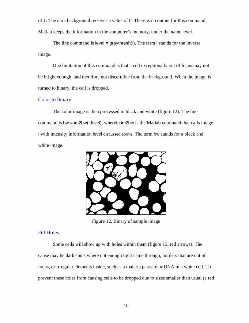
The color image is then processed to black and white (figure 12). The line

command is bw = im2bw(I,level), wherein im2bw is the Matlab command that calls image

I with intensity information level discussed above. The term bw stands for a black and

white image.

Figure 12. Binary of sample image

Fill Holes Some cells will show up with holes within them (figure 13, red arrows). The

cause may be dark spots where not enough light came through, borders that are out of

focus, or irregular elements inside, such as a malaria parasite or DNA in a white cell. To

prevent these holes from causing cells to be dropped due to sizes smaller than usual (a red

10

cell has approximately 40-60 pixels in these images; white cells are larger), a command is

used to fill them.

The line command is bw2 = imfill(bw,’holes’), wherein imfill is the Matlab command,

bw is the binary image, ‘holes’ tells Matlab to look for openings, cracks or fissures within bodies

(versus filling the entire image), and bw2 is the output (figure 14).

Figure 13. Presence of holes within cells Figure 14. Image after holes were filled

Open

11

The image at this point still has a few elements that are not relevant, including

parts of cells on the periphery of the image (figure 15, arrow 1), and other small elements

unknown to the author (arrows 2 and 3). To eliminate these items, a morphological

opening is performed, consisting of an erosion and a dilation of the elements on the

image (21-22). An essential part of these two operations is the structuring element

(named strel in the code) used to probe the input image (23). A two-dimensional, or flat,

structuring element consists of a matrix of 0's and 1's. The center pixel of the structuring

element, called the origin, identifies the pixel of interest — the pixel being processed.

The pixels in the structuring element containing 1's define the neighborhood of the

structuring element. These pixels are also considered in erosion or dilation processing. A

disk function is used to outline the shape of the cells — what the software is supposed to

examine, and a radius (number of pixels) is input as the minimum size of the

neighborhood. Anything smaller is eliminated.

3

2 1

Figure 15. Small elements in sample image 1. Part of a cell 2-3. Unknown elements After the neighborhood of pixels is defined, an erosion operation is performed

that modifies all pixels set as 1’s with the value 0, per the radius set by the user. See the

illustration in figures 16 and 17.

12

Figure 16. Original image (i.e. one cell)

Figure 17. Erosion of cell in image The next step of the open is a dilation of the image. See illustration in figure 18.

Figure 18. Dilation of cell in image

The command line is background = imopen(bw2,strel(‘disk’,20));

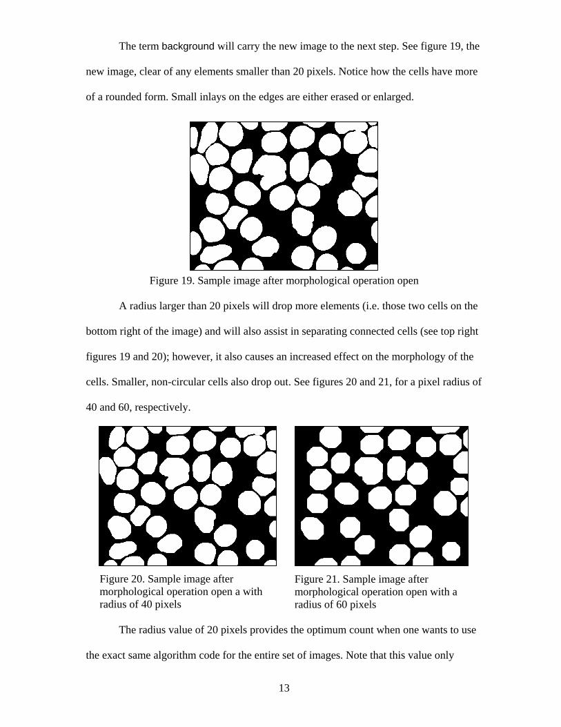
The term background will carry the new image to the next step. See figure 19, the

new image, clear of any elements smaller than 20 pixels. Notice how the cells have more

of a rounded form. Small inlays on the edges are either erased or enlarged.

Figure 19. Sample image after morphological operation open

A radius larger than 20 pixels will drop more elements (i.e. those two cells on the

bottom right of the image) and will also assist in separating connected cells (see top right

figures 19 and 20); however, it also causes an increased effect on the morphology of the

cells. Smaller, non-circular cells also drop out. See figures 20 and 21, for a pixel radius of

40 and 60, respectively.

Figure 20. Sample image after morphological operation open a with radius of 40 pixels

Figure 21. Sample image after morphological operation open with a radius of 60 pixels

The radius value of 20 pixels provides the optimum count when one wants to use

the exact same algorithm code for the entire set of images. Note that this value only

13

applies for the images analyzed for this project. Images taken with a different blood film

preparation, magnification, microscope, camera, set of lenses, etc. may have cells of

different sizes which require a different radius value.

Drop Cells on Borders Since it is often difficult to differentiate which type of cell is present on the

periphery of an image, the algorithm removes them.

The command line is nobrd = imclearborder(background,26). The largest distance

from the border that Matlab allows for analysis is 26 pixels; hence some cells stay in the

output (figure 22). Another limitation is observed in figures 19 and 22: cells away from

the border which are interconnected to cells on the border are also dropped.

Figure 22. Sample image after clear border command A third limitation involves the equipment used to take the images. One can notice

a thin black slit between the left side of the image above and the cells next to it. Since the

cells are not actually connected to the border (due to a lapse by the Olympus

hardware/software), they are never analyzed by the clear border command.

Count Cells

The Euler number command is used to count the number of cells. It functions by

considering patterns of convexity and concavity in local 2-by-2 pixel neighborhoods (20).

14

15

The command line is eul = bweuler(nobrd). The output for the image above is the eul

value 28. A manual count of the image indicates there are in fact 28 cells present.

A pre-count of each image was performed manually where only the cells not

touching the periphery of the image were considered. The sum for the image above

(number four in appendix C) was 28. Hence, while the algorithm erred in keeping certain

cells on the borders and dropping other interconnected cells, it still returned the true

count for this image. The implications of this output are detailed in the results and

discussion portion of the project.

Morphological Structuring This step involves creating a structuring element with a 25-pixel disk-shaped

radius of the inverse image. The command line is structure = strel(‘disk’,25);

The information structure will be used on the next step.

Two types of cells were found in the images: red and white cells. Red cells carry

oxygen from the lungs to the tissues around the body, and carbon dioxide from the tissues

to the lungs. White cells are responsible for protecting the body from germs or infections

(24-25). They do so by releasing protective antibodies that overpowers the germ, or

surround and devour the bacteria. The computer algorithm has to differentiate between

these two types of cells, since both infected red cells and white cells have DNA; which,

when stained, have the same color. Healthy red cells do not have DNA (figure 4). The

algorithm takes into account the different physical shapes of each cell by performing a

morphological top-hat filter on the inverse image using the structuring element structure

above.

Top-Hat Filtering

As the open removes narrow protrusions or spikes on the contour of cells, and

tiny elements altogether, the top-hat filter reveals exactly these residues that the

structuring element does not fit (26); hence, all the small elements inside sick red cells

come up stronger in the output than healthy red cells (figure 23), or the edges of white

cells (see appendix C, images 13 and 14).

Figure 23. Sample image after top-hat filter

The line command is Itop = imtophat(I,structure);

Level Threshold

At this point, the algorithm needs the global threshold value discussed earlier to

convert to binary. The line command is level = graythresh(Itop);

Color to Binary

Using the same method discussed earlier, the image is converted to binary (figure

24).

Figure 24. Binary of sample image with parasite

16

The line command is bw = im2bw(Itop,level);

Fill Holes

The holes are then filled to prevent the parasite from being dropped along with

other smaller elements during the open (figure 25).

17

Figure 25. Sample image with parasite and holes filled The line command is bw2 = imfill(bw,’holes’) This command also has limitations. Depending on the thickness of the edge of a

red cell, the fill hole command fills a healthy cell’s outline. Image 10 in appendix C

shows how a healthy cell out of focus can be counted as sick.

Open Figure 26 illustrates the result of an open with a pixel radius of 26.

Figure 26. Sample image with parasite after morphological operation open

18

A smaller radius will not drop enough of the remnant elements on the image;

while a larger radius will drop the smaller sick cells found in some images (see image 12

in appendix C).

The command line is background2 = imopen(bw2,strel(‘disk’,26);

Count Parasites Last step in the algorithm is an Euler number command. The command line is

eul = bweuler(background2). The output is 1; which is correct.

See appendix B for the entire algorithm code, and an index for each image in

appendix C. Appendix D has mathematical algorithms for the morphological operations

open and top-hat filter.

19

3. Results

Table 1 shows the number of cells in each image per a manual count by the author

(where only cells within the image boundaries are considered), whether there is a parasite

or not in each image, the algorithm output for the total number of cells (includes white

cells, and healthy and sick red cells), the actual number of sick cells, and the algorithm

output for the number of sick cells.

Photo Number

Sick (YES/NO)

Actual Count: Total

Number of Cells

Algorithm Count: Total

Number of Cells

Actual Number of Sick Cells

Algorithm Count of

Sick Cells

1 NO 25 24 0 0 2 YES 25 27 1 1 3 YES 24 24 1 1 4 YES 28 28 1 1 5 YES 24 30 1 1 6 NO 20 20 0 0 7 NO 15 15 0 0 8 NO 25 24 0 0 9 YES 13 14 1 1 10 YES 23 25 1 2 11 YES 30 30 1 1 12 YES 25 22 2 2 13 NO 21 17 0 0 14 NO 20 17 0 0 15 YES 34 37 2 2 16 YES 28 29 1 1 17 NO 16 16 0 0 18 NO 21 21 0 1 19 NO 19 19 0 0 20 NO 15 17 0 2 21 YES 23 28 0 0 22 NO 22 20 0 0 23 YES 18 18 1 1 24 YES 18 14 2 2 25 YES 27 28 1 1 26 YES 25 25 1 2

Table 1. Results of actual count and algorithm output

20

From the initial 32 images taken, only 26 were analyzed. Six images were

dropped because the algorithm could not process them, leading to inconclusive results.

There are three groups of reason that influenced this decision: blood film preparation,

quality of images, and algorithm design.

Blood film preparation considers lack of spacing between cells, and other

elements in the images the author could not identify. The better the spacing, the more

accurate the count.

Quality of images considers focus, and too much or too little lighting through

cells; hence they blend with the background. A set of images where every cell is in focus

provides for better results.

Algorithm design considers limitations by the algorithm that should be worked

out in future research.

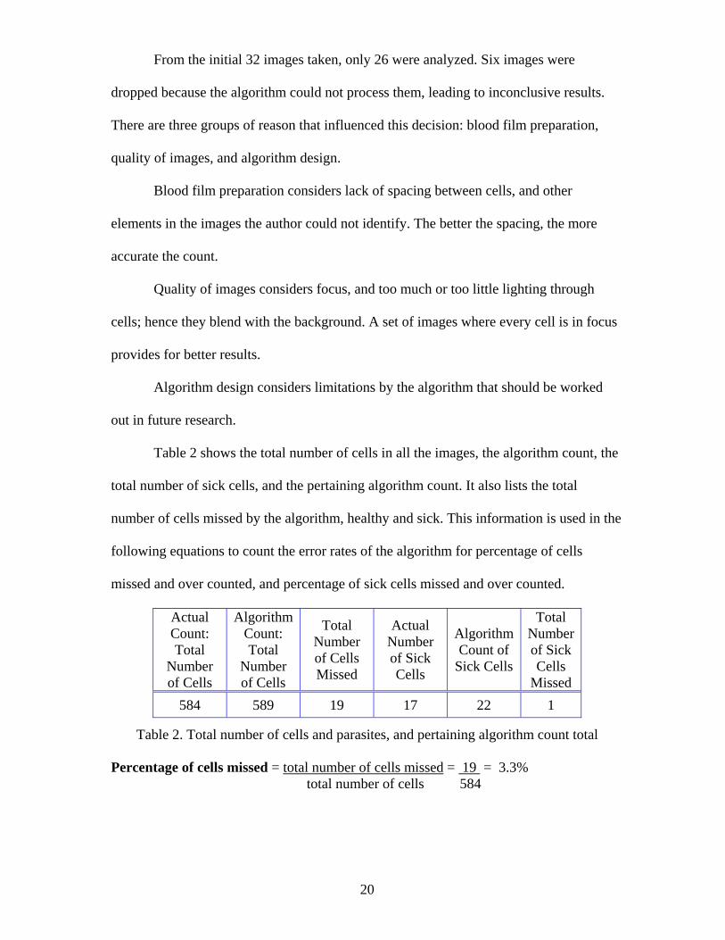
Table 2 shows the total number of cells in all the images, the algorithm count, the

total number of sick cells, and the pertaining algorithm count. It also lists the total

number of cells missed by the algorithm, healthy and sick. This information is used in the

following equations to count the error rates of the algorithm for percentage of cells

missed and over counted, and percentage of sick cells missed and over counted.

Actual Count: Total

Number of Cells

Algorithm Count: Total

Number of Cells

Total Number of Cells Missed

Actual Number of Sick Cells

Algorithm Count of

Sick Cells

Total Number of Sick Cells

Missed 584 589 19 17 22 1

Table 2. Total number of cells and parasites, and pertaining algorithm count total Percentage of cells missed = total number of cells missed = 19 = 3.3% total number of cells 584

21

The algorithm missed 3.3% of the cells due to physical contact between cells. A

lack of discernible separation between two cells is counted as one cell by the software.

The border drop command also dropped whole cells touching partial cells on the border.

Percentage of cells over counted = number of cells over counted = 77 = 13.2% total number of cells 584

Cells over counted came from the border of the images and small unidentified

elements. These were not counted in the manual count, hence the disparity of 13.2%.

Percentage of sick cell cells missed = total number of sick cells missed = 1 = 5.9% total number of cells 17

The algorithm missed one parasite in image number 12. The cell had very

dispersed elements and its binary cell image did not fill with the fill-hole command,

hence it was dropped after the open. Note that another healthy cell was recognized as sick

in the same image; thus, the correct count output for this image in table 1.

Percentage of sick cells over counted = number of sick cells over counted = 5 = 29.4% total number of sick cells 17

The algorithm erred in the count of sick cells by almost 30% over the actual

number. The use of blood smears prepared for computer image analysis would decrease

this number, due to overall better image quality. The blood smears available for this study

were prepared solely for visual microscopy by an expert in malarial analysis. More

emphasis on spacing between cells and an overall flat state by cells against the glass on

the background would diminish errors.

Appendix E has a table that quantifies the extent of the disease in each image with

a ratio of sick cells and the total number of cells; and appendix F has a table that provides

a quality analysis of the cell count with a ratio of the algorithm count and the actual cell

count by the author.

4. Discussion and Conclusions This study found that the use of computer image analysis of digital images to

count the number of cells and detect parasites in blood smears provides a valid diagnosis

tool for malaria. Di Ruberto and collaborators were the first researchers to use computer

image vision to detect malaria parasites. They used Matlab to count the number of cells

by use of gray scale granulometries, and detected parasites by means of an automatic

thresholding based on a morphological approach. In similar manner, this project uses

morphological operators to count the number of cells; however, it uses a top-hat filter to

detect parasites within cells. Both methods seem to provide similar results.

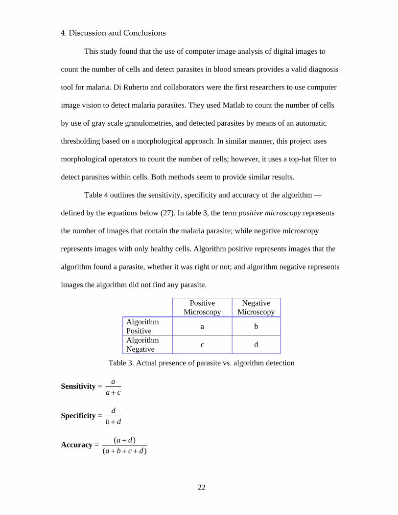
Table 4 outlines the sensitivity, specificity and accuracy of the algorithm —

defined by the equations below (27). In table 3, the term positive microscopy represents

the number of images that contain the malaria parasite; while negative microscopy

represents images with only healthy cells. Algorithm positive represents images that the

algorithm found a parasite, whether it was right or not; and algorithm negative represents

images the algorithm did not find any parasite.

Positive Microscopy

Negative Microscopy

Algorithm Positive a b

Algorithm Negative c d

Table 3. Actual presence of parasite vs. algorithm detection

Sensitivity = ca

a+

Specificity = db

d+

Accuracy = )(

)(dcba

da+++

+

22

23

Positive Microscopy Negative Microscopy

Parasite Algorithm Positive

Algorithm Negative

Algorithm Positive

Algorithm Negative

Sensitivity (%)

Specificity (%)

Accuracy (%)

P. vivax 14 0 2 10 100.0 83.3 92.3

Table 4. Sensitivity, specificity and accuracy of algorithm The algorithm has high sensitivity, which is desirable since one would like a test

of high success rate of detecting positive cases. Inability of the test to correctly identify a

true positive might result in missing potential cases of the disease. Conversely, the test is

not highly specific at 83.3%, hence there are false positives. Overall, the algorithm had an

accuracy of 92.3%, which is considered good under clinical parameters.

The algorithm developed to find and count parasites is a novel alternative to

current diagnostic methods. The software is able to find parasites in low quantities and

quantify the extent of infection, all in less than five minutes. However, the use of

computer image vision requires expensive equipment not available in many countries,

mainly those affected by the epidemics. Microscopy continues to be the gold standard for

the diagnosis of malaria.

24

5. Recommendations for Future Research As outlined in table 1, the algorithm over counted and under counted the number

of cells in certain images. It also counted some healthy red and white cells as sick with

parasites. To increase the accuracy of the output, and diminish type I and II errors, the

author suggests an algorithm that collects an array of results based on a large number of

cycles. The algorithm would adjust one factor per cycle, and compare the output with all

the previous runs until the results maintained some consistency; hence it would stop only

when it reached a pre-determined consensus value (i.e. ten equal cell counts). Factors

would include image brightness and contrast, open radius, structuring element radius for

the top-hat filter, and perhaps a color overlay for the inverse image. Shades of blue, as

seen in figure 11, might not provide the best basis for collection of thresholding

information to binary.

Furthermore, the preparation of the blood smears needs to take into account the

purpose of the sample. The better the spacing between cells, the less likely the chance of

type I and II errors; where multiple cells were counted as one, and one or more cells were

dropped. Images out of focus should be discarded; and either the imaging equipment

should not leave gaps on the border of images, or the gap between cells and the border

should be automatically shortened.

25

Appendix A — Equipment Specifications System Microscope Olympus BX60 Lenses: Olympus 10X, 20X, 40X, 100X Optical Characteristics:

Eyepiece WH10X

Magnification Resolution (µm) Total Magnification

Depth of Focus (µm)

Field of View

10X 1.34 100X 28.0 2.2 20X 0.84 200X 6.09 1.1 40X 0.52 400X 3.04 0.55 100X 0.27 1000X 0.69 0.22

Digital Camera Olympus DEI-750D Digital Output Model 60660 Image Sensor: 3 x ½” CCD-chip, one per color channel Picture Format: 6.4 mm x 4.8 mm Internal lens: f 1.4, primary color (RGB) Picture Elements (NTSC): 768 x 582 pixels per chip, 1,138,176 in total Software Adobe Photoshop 6.5 (for dust removal and image inverse) Microsoft Excel 2003 The MathWorks Matlab 6.5.0.1924 Release 13 Image Processing Toolbox 4.1

26

Appendix B — Matlab Algorithm

Code Image Output (see appendix C)

Count Output (see appendix C)

clear I = imread('filename.png'); level = graythresh(I); bw = im2bw(I,level); figure, imshow(bw) bw2 = imfill(bw,'holes') figure, imshow(bw2) background = imopen(bw2,strel('disk',20)); figure, imshow(background) nobrd = imclearborder(background,26) figure, imshow(nobrd) eul = bweuler(nobrd) structure = strel('disk', 25); Itop = imtophat(I, structure); figure, imshow(Itop, []) level = graythresh(Itop); bw = im2bw(Itop,level); figure, imshow(bw) bw2 = imfill(bw,'holes') figure, imshow(bw2) background2 = imopen(bw2,strel('disk',26)); figure, imshow(background2) eul = bweuler(background2)

1 2 3 4 5 6 7 8

Cell Count

Parasites Count

27

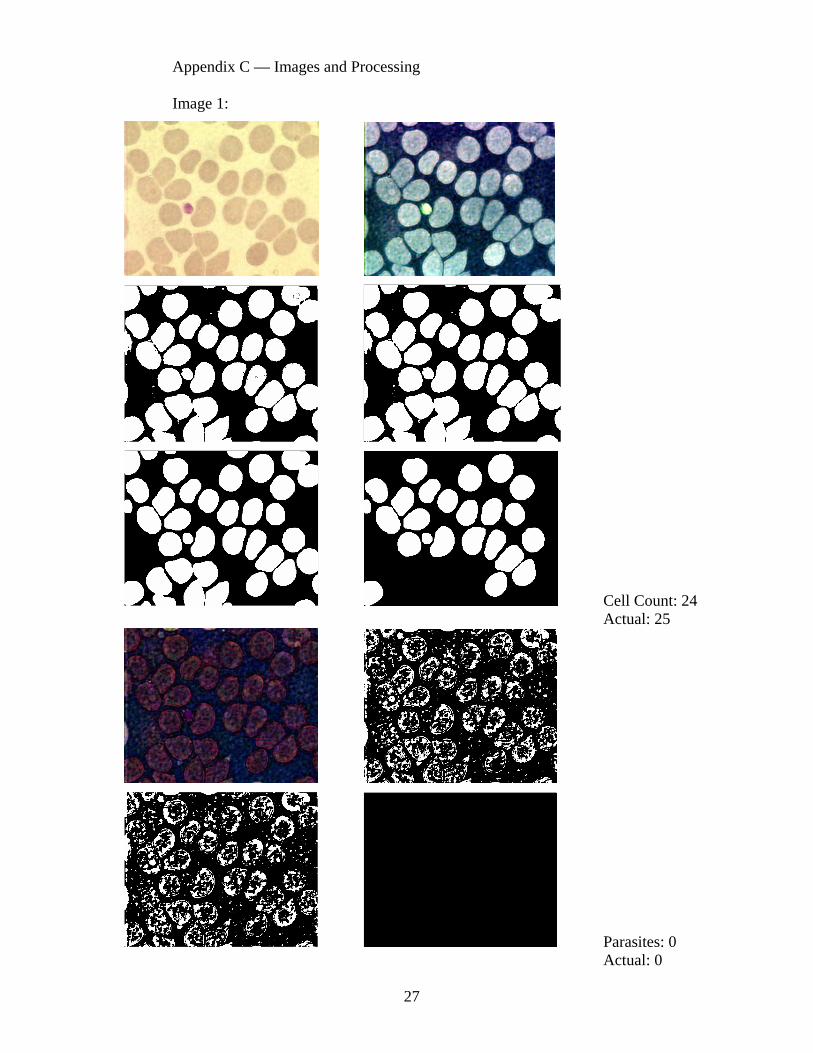
Appendix C — Images and Processing Image 1:

Cell Count: 24 Actual: 25

Parasites: 0 Actual: 0

28

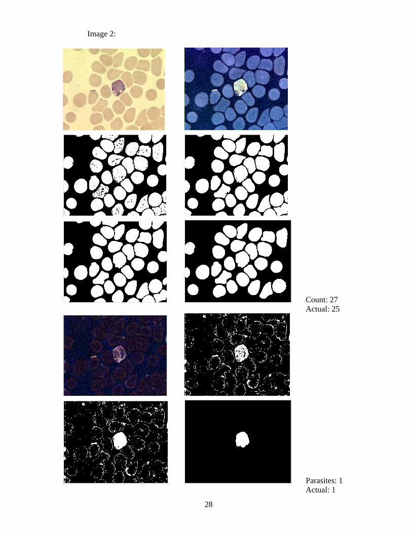
Image 2:

Count: 27 Actual: 25


29

Image 3:



30

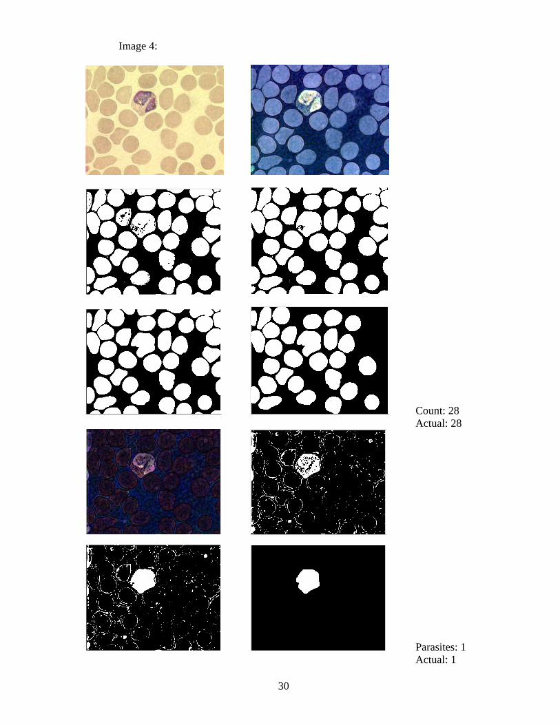
Image 4:



31

Image 5:



32

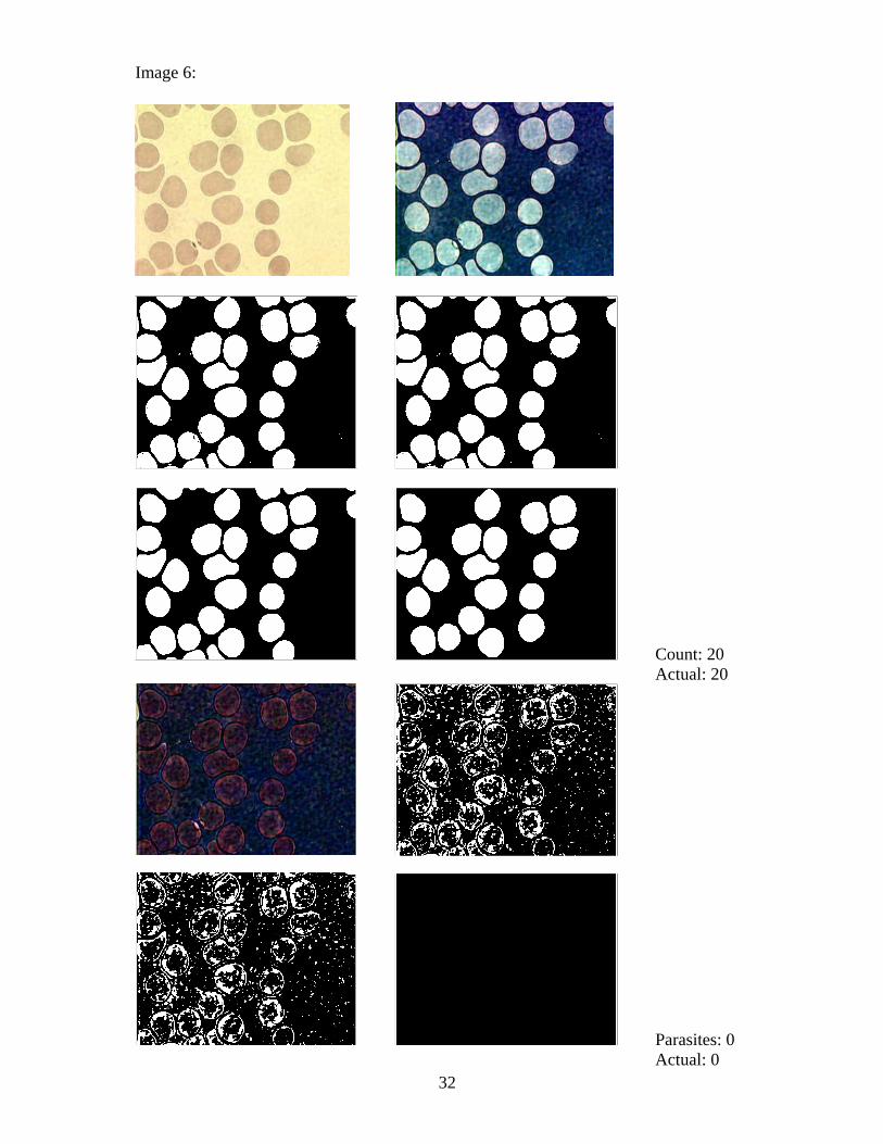
Image 6:



33

Image 7:



34

Image 8:



35

Image 9:


Parasite: 1 Actual: 1

36

Image 10:



37

Image 11:



38

Image 12:


Parasite: 2 Actual: 2

39

Image 13:



40

Image 14:


Count: 0 Actual: 0

41

Image 15:



42

Image 16:



43

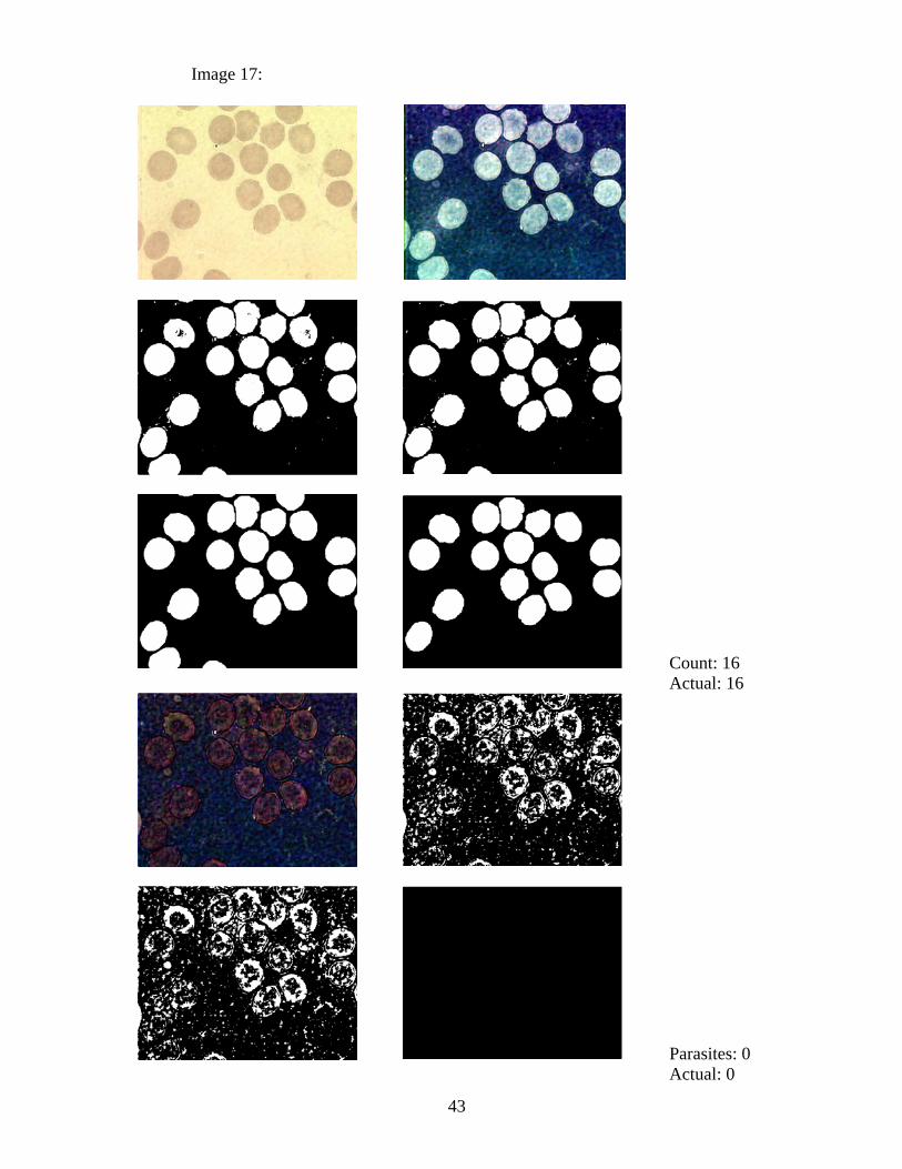
Image 17:



44

Image 18:



45

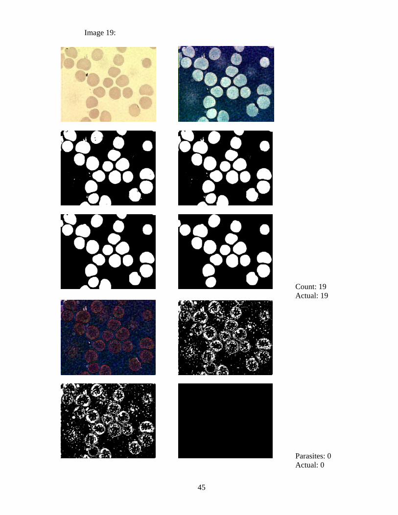
Image 19:



46

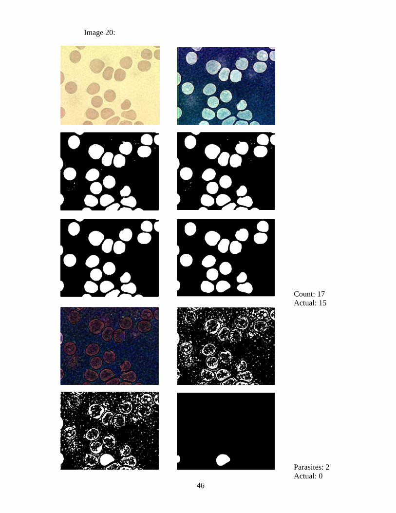
Image 20:



47

Image 21:



48

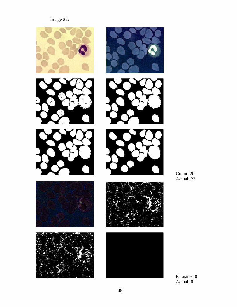
Image 22:



49

Image 23:



50

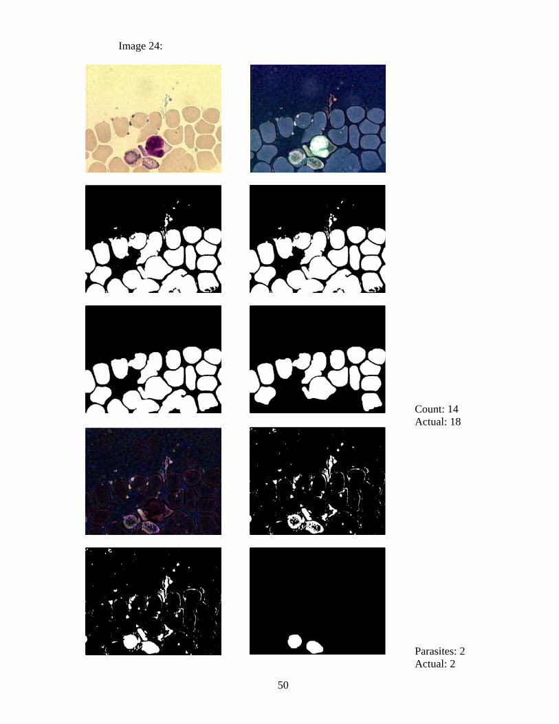
Image 24:



51

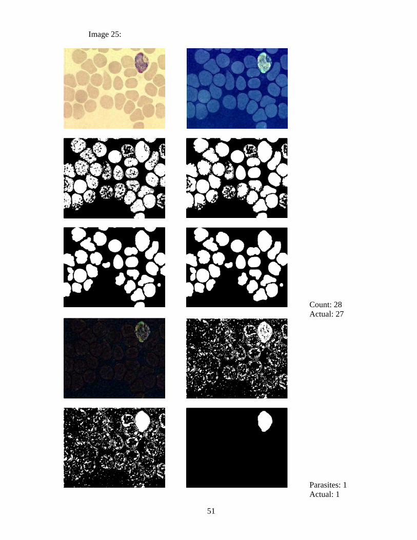
Image 25:



52

Image 26:



53

Appendix D — Mathematical Algorithms

Open

The eroded image of an object O with respect to a structuring element S with a reference point R, , is the set of all reference points for which S is completely contained in O.

The dilated image of an object O with respect to a structuring element S with a reference point R, , is the set of all reference points for which O and S have at least one common point.

Opening is defined as an erosion, followed by a dilation: .

Closing is defined as a dilation, followed by an erosion: .

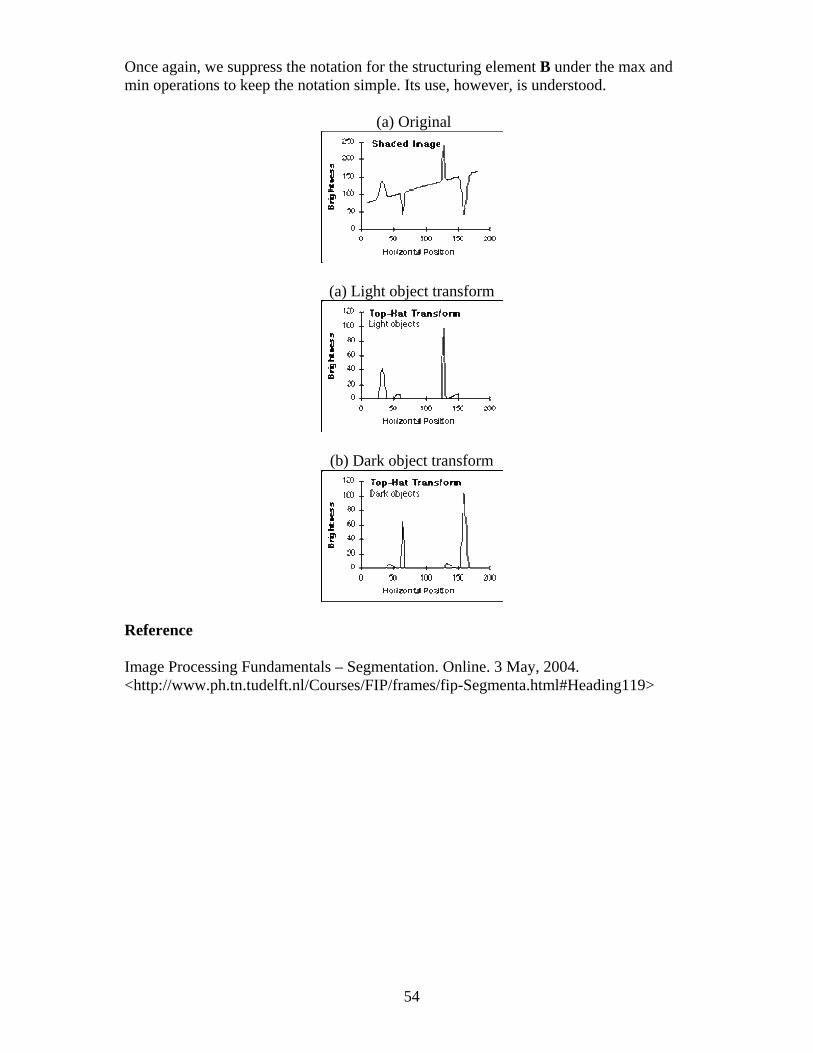
Reference Morphological Operators. Online. 3 May 2004. < http://rkb.home.cern.ch/rkb/AN16pp/node178.html> Top-Hat Filter The isolation of gray-value objects that are convex can be accomplished with the top-hat transform. Depending upon whether we are dealing with light objects on a dark background or dark objects on a light background, the transform is defined as: Light objects - Dark objects - where the structuring element B is chosen to be bigger than the objects in question and, if possible, to have a convex shape. Because of the properties given in equations and, TopHat(A,B) > 0. An example of this technique is shown in the following figure. The original image including shading is processed by a 15 x 1 structuring element as described in eqs. and to produce the desired result. Note that the transform for dark objects has been defined in such a way as to yield "positive" objects as opposed to "negative" objects. Other definitions are, of course, possible. Thresholding A simple estimate of a locally-varying threshold surface can be derived from morphological processing as follows: Threshold surface -

54

Once again, we suppress the notation for the structuring element B under the max and min operations to keep the notation simple. Its use, however, is understood.

(a) Original

(a) Light object transform

(b) Dark object transform

Reference Image Processing Fundamentals – Segmentation. Online. 3 May, 2004. <http://www.ph.tn.tudelft.nl/Courses/FIP/frames/fip-Segmenta.html#Heading119>

55

Appendix E — Ratio of Algorithm Cell Count and Actual Sick Cell Count

Photo Number

Sick (YES/NO)

Algorithm Count of Total Number of Cells

Algorithm Count of Sick Cells

Extent of Disease Ratio

1 NO 24 0 NA 2 YES 27 1 3.70% 3 YES 24 1 4.17% 4 YES 28 1 3.57% 5 YES 30 1 3.33% 6 NO 20 0 NA 7 NO 15 0 NA 8 NO 24 0 NA 9 YES 14 1 7.14% 10 YES 25 2 8.00% 11 YES 30 1 3.33% 12 YES 22 2 9.09% 13 NO 17 0 NA 14 NO 17 0 NA 15 YES 37 2 5.41% 16 YES 29 1 3.45% 17 NO 16 0 NA 18 NO 21 1 4.76% 19 NO 19 0 NA 20 NO 17 2 11.76% 21 YES 28 0 NA 22 NO 20 0 NA 23 YES 18 1 5.56% 24 YES 14 2 14.29% 25 YES 28 1 3.57% 26 YES 25 2 8.00%

The ratio is wrong for images 18 and 20; since there are, in fact, no parasites in

those images.

Extent of Disease Ratio = Algorithm Count of Sick Cells Algorithm Count

56

Appendix F — Ratio of Algorithm Count and Actual Cell Count

Photo Number

Sick (YES/NO)

Actual Count

Algorithm Count Cell Count Ratio

1 NO 25 24 96.00% 2 YES 25 27 108.00% 3 YES 24 24 100.00% 4 YES 28 28 100.00% 5 YES 24 30 125.00% 6 NO 20 20 100.00% 7 NO 15 15 100.00% 8 NO 25 24 96.00% 9 YES 13 14 107.69% 10 YES 23 25 108.70% 11 YES 30 30 100.00% 12 YES 25 22 88.00% 13 NO 21 17 80.95% 14 NO 20 17 85.00% 15 YES 34 37 108.82% 16 YES 28 29 103.57% 17 NO 16 16 100.00% 18 NO 21 21 100.00% 19 NO 19 19 100.00% 20 NO 15 17 113.33% 21 YES 23 28 121.74% 22 NO 22 20 90.91% 23 YES 18 18 100.00% 24 YES 18 14 77.78% 25 YES 27 28 103.70% 26 YES 25 25 100.00%

Cell Count Ratio = Algorithm Count Actual Count

57

Appendix G — Definition of Algorithm Commands

The following command descriptions come from MathWorks’ web site: < http://www.mathworks.com > graythresh

Compute global image threshold using Otsu's method

Syntax

• level = graythresh(I) Description

level = graythresh(I) computes a global threshold (level) that can be used to convert an intensity image to a binary image with im2bw.

The graythresh function uses Otsu's method, which chooses the threshold to minimize the intraclass variance of the black and white pixels.

Class Support

The input image I can be of class uint8, uint16, or double and it must be nonsparse. The return value level is a double scalar.

Reference

Otsu, N., "A Threshold Selection Method from Gray-Level Histograms," IEEE Transactions on Systems, Man, and Cybernetics, Vol. 9, No. 1, 1979, pp. 62-66.

im2bw

Convert an image to a binary image, based on threshold

Syntax

• BW = im2bw(I,level) Description

im2bw produces binary images from indexed, intensity, or RGB images. To do this, it converts the input image to grayscale format (if it is not already an intensity image), and then uses thresholding to convert this grayscale image to binary. The output binary image BW has values of 0 (black) for all pixels in the input image with luminance less than level and 1 (white) for all other pixels. (Note that you specify level in the range [0,1], regardless of the class of the input image.)

BW = im2bw(I,level) converts the intensity image I to black and white.

Note The function graythresh can be used to compute the level argument automatically.

58

Class Support

The input image can be of class uint8, uint16, or double and it must be nonsparse. The output image, BW, is of class logical.

imfill

Fill image regions

Syntax

• BW2 = imfill(BW,locations) • BW2 = imfill(BW,'holes') • I2 = imfill(I)

Description

BW2 = imfill(BW,locations) performs a flood-fill operation on background pixels of the binary image BW, starting from the points specified in locations. If locations is a P-by-1 vector, it contains the linear indices of the starting locations. If locations is a P-by-ndims(BW) matrix, each row contains the array indices of one of the starting locations.

BW2 = imfill(BW,'holes') fills holes in the binary image BW. A hole is a set of background pixels that cannot be reached by filling in the background from the edge of the image.

I2 = imfill(I) fills holes in the intensity image I. In this case, a hole is an area of dark pixels surrounded by lighter pixels.

Class Support

The input image can be numeric or logical, and it must be real and nonsparse. It can have any dimension. The output image has the same class as the input image.

Algorithm

imfill uses an algorithm based on morphological reconstruction.

Reference

Soille, P., Morphological Image Analysis: Principles and Applications, Springer-Verlag, 1999, pp. 173-174.

imopen

Open an image

Syntax

• IM2 = imopen(IM,SE) • IM2 = imopen(IM,NHOOD)

59

Description

IM2 = imopen(IM,SE) performs morphological opening on the grayscale or binary image IM with the structuring element SE. The argument SE must be a single structuring element object, as opposed to an array of objects.

IM2 = imopen(IM,NHOOD) performs opening with the structuring element strel(NHOOD), where NHOOD is an array of 0's and 1's that specifies the structuring element neighborhood.

Class Support

IM can be any numeric or logical class and any dimension, and must be nonsparse. If IM is logical, then SE must be flat. IM2 has the same class as IM.

imclearborder

Suppress light structures connected to image border

Syntax

• IM2 = imclearborder(IM) Description

IM2 = imclearborder(IM) suppresses structures that are lighter than their surroundings and that are connected to the image border. IM can be an intensity or binary image. The output image, IM2, is intensity or binary, respectively. The default connectivity is 8 for two dimensions, 26 for three dimensions, and conndef(ndims(BW),'maximal') for higher dimensions.

Note For intensity images, imclearborder tends to reduce the overall intensity level in addition to suppressing border structures.

Class Support

IM can be a numeric or logical array of any dimension, and it must be nonsparse and real. IM2 has the same class as IM.

Algorithm

imclearborder uses morphological reconstruction where

• Mask image is the input image. • Marker image is zero everywhere except along the border, where it equals the mask

image.

Reference

Soille, P., Morphological Image Analysis: Principles and Applications, Springer, 1999, pp. 164-165.

60

bweuler

Compute the Euler number of a binary image

Syntax

• eul = bweuler(BW,n) Description

eul = bweuler(BW,n) returns the Euler number for the binary image BW. The return value eul is a scalar whose value is the total number of objects in the image minus the total number of holes in those objects. The argument n can have a value of either 4 or 8, where 4 specifies 4-connected objects and 8 specifies 8-connected objects; if the argument is omitted, it defaults to 8.

Class Support

BW can be numeric or logical and it must be real, nonsparse, and two-dimensional. The return value eul is of class double.

Algorithm

bweuler computes the Euler number by considering patterns of convexity and concavity in local 2-by-2 neighborhoods. See ¥ for a discussion of the algorithm used.

References

Horn, Berthold P. K., Robot Vision, New York, McGraw-Hill, 1986, pp. 73-77.

¥ Pratt, William K., Digital Image Processing, New York, John Wiley & Sons, Inc., 1991, p. 633.

strel

Create morphological structuring element

Syntax

• SE = strel(shape,parameters) Description

SE = strel(shape,parameters) creates a structuring element, SE, of the type specified by shape. This table lists all the supported shapes. Depending on shape, strel can take additional parameters. See the syntax descriptions that follow for details about creating each type of structuring element.

Flat Structuring Elements

'arbitrary' 'pair'

'diamond' 'periodicline'

'disk' 'rectangle'

61

'line' 'square'

'octagon'

SE = strel('diamond',R) creates a flat, diamond-shaped structuring element, where R specifies the distance from the structuring element origin to the points of the diamond. R must be a nonnegative integer scalar.

SE = strel('disk',R,N) creates a flat, disk-shaped structuring element, where R specifies the radius. R must be a nonnegative integer. N must be 0, 4, 6, or 8. When N is greater than 0, the disk-shaped structuring element is approximated by a sequence of N periodic-line structuring elements. When N equals 0, no approximation is used, and the structuring element members consist of all pixels whose centers are no greater than R away from the origin. If N is not specified, the default value is 4.

Note Morphological operations run much faster when the structuring element uses approximations (N > 0) than when it does not (N = 0). However, structuring elements that do not use approximations (N = 0) are not suitable for computing granulometries. Sometimes it is necessary for strel to use two extra line structuring elements in the approximation, in which case the number of decomposed structuring elements used is N + 2.

SE = strel('line',LEN,DEG) creates a flat, linear structuring element, where LEN specifies the length, and DEG specifies the angle (in degrees) of the line, as measured in a counterclockwise direction from the horizontal axis. LEN is approximately the distance between the centers of the structuring element members at opposite ends of the line.

62

SE = strel('octagon',R) creates a flat, octagonal structuring element, where R specifies the distance from the structuring element origin to the sides of the octagon, as measured along the horizontal and vertical axes. R must be a nonnegative multiple of 3.

Notes

For all shapes except 'arbitrary', structuring elements are constructed using a family of techniques known collectively as structuring element decomposition. The principle is that dilation by some large structuring elements can be computed faster by dilation with a sequence of smaller structuring elements. For example, dilation by an 11-by-11 square structuring element can be accomplished by dilating first with a 1-by-11 structuring element and then with an 11-by-1 structuring element. This results in a theoretical performance improvement of a factor of 5.5, although in practice the actual performance improvement is somewhat less. Structuring element decompositions used for the 'disk' and 'ball' shapes are approximations; all other decompositions are exact.

Algorithm

The method used to decompose diamond-shaped structuring elements is known as "logarithmic decomposition" [1].

The method used to decompose disk structuring elements is based on the technique called "radial decomposition using periodic lines" [2], [3]. For details, see the MakeDiskStrel subfunction in toolbox/images/images/@strel/strel.m.

The method used to decompose ball structuring elements is the technique called "radial decomposition of sphere" [2].

63

References

[1] van den Boomgard, Rein, and Richard van Balen, "Methods for Fast Morphological Image Transforms Using Bitmapped Images," Computer Vision, Graphics, and Image Processing: Graphical Models and Image Processing, Vol. 54, No. 3, May 1992, pp. 252-254.

[2] Adams, Rolf, "Radial Decomposition of Discs and Spheres," Computer Vision, Graphics, and Image Processing: Graphical Models and Image Processing, Vol. 55, No. 5, September 1993, pp. 325-332.

[3] Jones, Ronald, and Pierre Soille, "Periodic lines: Definition, cascades, and application to granulometrie," Pattern Recognition Letters, Vol. 17, 1996, pp. 1057-1063.

imtophat

Perform top-hat filtering

Syntax

• IM2 = imtophat(IM,SE) • IM2 = imtophat(IM,NHOOD)

Description

IM2 = imtophat(IM,SE) performs morphological top-hat filtering on the grayscale or binary input image IM using the structuring element SE, where SE is returned by strel. SE must be a single structuring element object, not an array containing multiple structuring element objects.

IM2 = imtophat(IM,NHOOD), where NHOOD is an array of 0's and 1's that specifies the size and shape of the structuring element, is the same as imptophat(IM,strel(NHOOD)).

Class Support

IM can be numeric or logical and must be nonsparse. The output image IM2 has the same class as the input image. If the input is binary (logical), the structuring element must be flat.

64

7. References

1. What is Malaria? Roll Back Malaria. Online. 26 December 2003. <http://www.rbm.who.int>

2. Malaria: Laboratory Diagnosis. Online. 25 December 2003. <http://www.rph.wa.gov.au>

3. World Health Organization. A rapid dipstick antigen capture assay for the diagnosis of falciparum malaria. 74.11 (1996) 47-54

4. Bernard Henry, John. Clinical Diagnosis & Management, by Laboratory Methods. W.B. Saunders Company. Philadelphia (1991) 1168-1172

5. CJ Palmer, JA Bonilla, DA Bruckner, NS Miller, MA Haseeb, JR Masci, WM Stauffer. Multicenter study to evaluate the OptiMAL test for rapid diagnosis of malaria in U.S. Hospitals. Journal of Clinical Microbiology. 41.11 (November 2003) 5178-5182

6. J Iqbal, N Khalid, PR Hira. Comparison of two commercial assays with expert microscopy for confirmation of symptomatically diagnosed malaria. Journal of Clinical Microbiology. 40.12 (December 2002) 4675-4678

7. MH Craig, BL Bredenkamp, CH Vuaghan William, EJ Rossouw, VJ Kelly, I Kleinschmidt, A Martineau, and GFJ Henry. Field and laboratory comparative evaluation of ten rapid malaria diagnostic tests. Transactions of the Royal Society of Tropical Medicine and Hygiene. 96 (2002) 258-265

8. RE Coleman, N Maneechai, A Ponlawat, C. Kumptitak, N Rachapaew, RS Miller, and J Sattabongkot. Short report: failure of the OptiMAL rapid malaria test as a tool for the detection of asymptomatic malaria in an area of Thailand endemic for plasmodium falciparum and p. vivax. American Society of Tropical Medicine and Hygiene. 67.6 (2002) 563-565

9. H Voigt, and Classen R. Topodermatographic Image Analysis for Melanoma Screening and the Quantitative Assessment of Tumor Dimension Parameters of the Skin. Cancer. 75.4 (15 February, 1995) 981-988

10. JF Aitken, J Pfitzner, D Battistutta, PK O’Rourke, AC Green, NG Martin. Reliability of computer image analysis of pigmented skin lesions of Australian adolescents. Cancer. 78.2 (15 July, 1996) 252-257

11. TW Nattkemper, T Twellmann, H Ritter, W Schubert. Human vs. Machine: Evaluation of Fluorescence Micrographs. Computer in Biology and Medicine. 33 (2003) 31-43

12. H Satelet, O Garraud, M Lorenzato, C Rogier, I Milko-Sartelet, M Huerre, and D Gaillard. Quantitative Computer Image Analysis of Chondroitin Sulfate A Expression in Placentas Infected with Plasmodium Falciparum. The Journal of Histochemistry & Cytochemistry. 47.6 (1999) 751-756

13. Mohamed Sammouda, Rachid Sammouda, Noboru Niki, Kiyoshi Mukai. Liver cancer detection system based on the analysis of digitized color images of tissue samples obtained using needle biopsy. Information Visualization. 1.2 (Jun 2002) 130

14. R. Barthelson, C Hopkins, and A Mobasseria. Quantitation of bacterial adherence by image analysis. American Journal of Microbiological Methods. 38.1-2 (October 1999) 17-23

15. C Di Ruberto, A Dempster, S Khan, B Jarra. Analysis of Infected Blood Cell Images using Morphological Operators. Image and Vision Computing. 20 (2002) 20133-20146

65

16. Watershed Algorithm. Online. 10 April, 2004. <http://rsb.info.nih.gov/ij/plugins/watershed.html>

17. G. Adelmann, Holger. Butterworth Equations for Homorphic Filtering of Images. Computers in Biology and Medicine. 28 (1998) 169-181

18. CR Garcia, AR Dluzewski, LH Catalani, R Burting, J Hoyland, and WT Mason. Calcium Homestasic in Intraerythrocytic Malaria Parasites. European Journal of Cell Biology. 71.4 (December 1996) 409-13

19. Intro to PNG Features. Online. 29 March, 2004. <http://www.libpng.org/pub/png/pngintro.html>

20. Matlab 6.5 Help Reference. Software. 21. Morphological Operations. Online. 26 March 2004.

<http://rkb.home.cern.ch/rkb/AN16pp/node178.html> 22. What Are Morphological Operations? Online. 26 March 2004.

<http://developer.apple.com/documentation/Performance/Conceptual/vImage/ Chapter5/>

23. Structuring Elements :: Morphological Operations (Image Processing Toolbox). Online. 19 April, 2004. <http://www.mathworks.com/access/helpdesk/help/toolbox/images/morph5.ht ml#22581>

24. Battling Blood Cells. Online. 28 March, 2004. <http://sln.fi.edu/biosci/blood/white.html>

25. Blood Cells. Online. 28 March, 2004. <http://www.drhull.com/EncyMaster/B/blood_cells.html>

26. Residues. Online. 30 April 2004. <http:www.mmorph.com/mmtutor1.0/html/mmtutor/mm045residues.html>

27. Sensitivity and Specificity. Online. 2 May 2004. <http://www.poems.msu.edu/InfoMastery/Diagnosis/SensSpec.htm>

Documents

Computer Image Analysis of Malarial Plasmodium …photos.imageevent.com/slo007/miscellaneous/projects/...Computer Image Analysis of Malarial Plasmodium Vivax in Human Red Blood Cells