Embed Size (px)
Citation preview

Computational
Model Order Reduction
of
Linear and Nonlinear
Dynamical Systems
- An Introduction -
Marcus Meyer
February 28, 2006

Contents
1 Introduction 11.1 The idea of computational model order reduction . . . . . . . . . . . . . . 11.2 Application examples . . . . . . . . . . . . . . . . . . . . . . . . . . . . . . 3
1.2.1 Fatigue simulation of wind turbines . . . . . . . . . . . . . . . . . . 31.2.2 NVH analysis of automobiles . . . . . . . . . . . . . . . . . . . . . . 31.2.3 Simulation of MEMS . . . . . . . . . . . . . . . . . . . . . . . . . . 3
2 Basic Mathematical Concepts 42.1 The Row/Column Picture of Linear Systems . . . . . . . . . . . . . . . . . 42.2 Least Squares Approximation . . . . . . . . . . . . . . . . . . . . . . . . . 52.3 The Singular Value Decomposition . . . . . . . . . . . . . . . . . . . . . . 8
2.3.1 Image approximation using the SVD . . . . . . . . . . . . . . . . . 102.3.2 SVD and Covariances . . . . . . . . . . . . . . . . . . . . . . . . . . 11
2.4 Problems . . . . . . . . . . . . . . . . . . . . . . . . . . . . . . . . . . . . . 13
3 Model order reduction techniques 153.1 Projection-based model reduction . . . . . . . . . . . . . . . . . . . . . . . 15
3.1.1 Example 1: CMOR of a linear system of 2nd order . . . . . . . . . 173.1.2 Example 2:CMOR of a nonlinear system . . . . . . . . . . . . . . . 183.1.3 Model reduction in variational form . . . . . . . . . . . . . . . . . . 18
3.2 Choices for the basis . . . . . . . . . . . . . . . . . . . . . . . . . . . . . . 203.2.1 Modal basis . . . . . . . . . . . . . . . . . . . . . . . . . . . . . . . 213.2.2 Lanczos basis . . . . . . . . . . . . . . . . . . . . . . . . . . . . . . 243.2.3 Proper Orthogonal Decomposition . . . . . . . . . . . . . . . . . . . 253.2.4 The recipe for the POD basis . . . . . . . . . . . . . . . . . . . . . 26
3.3 Problems . . . . . . . . . . . . . . . . . . . . . . . . . . . . . . . . . . . . . 27
4 Time discretization of the reduced model 294.1 Explicit Euler Time Integration . . . . . . . . . . . . . . . . . . . . . . . . 304.2 Implicit Euler Time Integration . . . . . . . . . . . . . . . . . . . . . . . . 304.3 Newmark method for 2nd order systems . . . . . . . . . . . . . . . . . . . 314.4 cG(q) time discretization . . . . . . . . . . . . . . . . . . . . . . . . . . . . 34
I

5 Improving the accuracy of the reduced model 365.1 Static Correction Method . . . . . . . . . . . . . . . . . . . . . . . . . . . 365.2 Nonlinear and Postprocessed Galerkin method . . . . . . . . . . . . . . . . 38
5.2.1 Invariant manifolds . . . . . . . . . . . . . . . . . . . . . . . . . . . 395.2.2 The center manifold . . . . . . . . . . . . . . . . . . . . . . . . . . 405.2.3 Inertial manifolds and the nonlinear Galerkin method . . . . . . . . 405.2.4 The nonlinear Galerkin method . . . . . . . . . . . . . . . . . . . . 425.2.5 Postprocessed Galerkin method . . . . . . . . . . . . . . . . . . . . 435.2.6 Approximate inertial manifolds . . . . . . . . . . . . . . . . . . . . 435.2.7 Nonlinear Galerkin method and Newmark time integration . . . . . 44
6 Error Estimation 466.1 The dual-weighted-residual method . . . . . . . . . . . . . . . . . . . . . . 486.2 Approximation of a linear equation . . . . . . . . . . . . . . . . . . . . . . 486.3 DWR for nonlinear functionals . . . . . . . . . . . . . . . . . . . . . . . . . 506.4 DWR for nonlinear systems . . . . . . . . . . . . . . . . . . . . . . . . . . 506.5 DWR for dynamical systems . . . . . . . . . . . . . . . . . . . . . . . . . . 51
6.5.1 Linear dynamical systems . . . . . . . . . . . . . . . . . . . . . . . 516.5.2 Nonlinear dynamical system . . . . . . . . . . . . . . . . . . . . . . 53
6.6 Approximation of model reduction and time discretization errors . . . . . . 536.7 Choice of proper basis vectors . . . . . . . . . . . . . . . . . . . . . . . . . 54
A A Short Linear Algebra Refresher 56A.1 Vector Spaces and Bases . . . . . . . . . . . . . . . . . . . . . . . . . . . . 56A.2 Norms, Inner Products and Orthogonality . . . . . . . . . . . . . . . . . . 57A.3 Linear Transformations . . . . . . . . . . . . . . . . . . . . . . . . . . . . . 59A.4 Useful Matrix Decompositions . . . . . . . . . . . . . . . . . . . . . . . . . 59
A.4.1 Eigendecomposition of A . . . . . . . . . . . . . . . . . . . . . . . . 59A.4.2 Singular value decomposition . . . . . . . . . . . . . . . . . . . . . 60
II

Chapter 1Introduction
Modeling and simulation of dynamical systems is a very important task in the engineeringsciences - and differential equations have proven to be one of the most sucessful means ofmodeling such systems. If the modeling is based on a first-principles approach, for examplewhen using the Finite Element or Finite Volume Method, the resulting mathematicalmodel is often too complicated or too time-consuming to compute, and thus not veryuseful in many practical applications. To obtain a simpler model, we basically have twochoices:
• The use of experience and engineering intuition to generate a simpler and thus moretractable model, or
• to employ approximation procedures based on mathematics to perform the modelreduction.
This course will exclusively deal with the second approach: The field of computationalmodel order reduction (CMOR) is concerned with the automatic model reduction ofdynamical systems described by ordinary differential equations or ordinary differential-algebraic equations.
1.1 The idea of computational model order reduction
Model reduction has a long history in the systems and control as well as the structuraldynamics community. Starting from a system of partial differential equations (PDE),which adequately describes the physical behaviour of the system under consideration, thespatial discretization of the PDE yields a system of ordinary differential equations (ODE).The dimension of this ODE system is governed by the spatial mesh size. Thus the finerthe mesh, the larger will be the dimension of the resulting system of ODEs, i.e. the morevariables occur that have to be solved in time. Depending on the dimension of the originalPDE and the desired spatial accuracy, the number of variables can extend from hundredsto several millions. If the interest lies in the time response of the system, as in the fieldsof structural and fluid dynamics, now this large system of ODEs has to be integrated intime to obtain the solution of the system: Solving for the time response of the systemmeans tracking the time evolution of the very many variables of the system of ODEs.This can be a large, sometimes prohibitive computational effort, even today.
1

1. Choosingthe basis
2. Projecting 3. Deforming thesubspace
subspaceon "flat"
time integration
PDEof ODEs
large system small system
of ODEs
approximated
solution
model reduction
spatial discretization
Figure 1.1: Projection-based model reduction.
Now model order reduction comes into the picture: Starting point for the modelreduction process will be the large system of ODEs
x = f(x, t), x ∈ RN , (1.1)
that results from the spatial discretization of the PDE, which we want to approximatewith a simpler (smaller) model of the form
ξ = g(ξ, t), ξ ∈ Rm. (1.2)
The first requirement of model order reduction is that the number of states m, i.e. thenumber of differential equations of the reduced model given by eq. (1.2), is much smalleras the number of states N of the original model in eq. (1.1),
m N. (1.3)
In the absense of additional requirements, this would be easy to satisfy by just eliminatingequations and state variables - the difficulty arises by imposing additional constraints, suchas:
1. The approximation error should be small, a global error bound should exist.
2. The procedure of model reduction should be computationally efficient.
3. The procedure of model reduction should be automatic, based on the error tolerance.
4. Important system properties like stability and passivity should be preserved.
In the following chapters we will describe methods which automatically generate asmaller (reduced) model of the large system of ODEs, which approximates the original
2

dynamical system in an adequate way. By a reduced model we mean a model that hasfewer states (inner or free variables) than the original model, i.e. a reduced model order.The secret lies in the transformation from the original to the reduced model: If you takea look a structural dynamics or fuid dynamics, you will see that often only a few largescale structures dominate the system response. These can be eigenmodes of a vibratingstructure or the eddies seen in a turbulent flow. These are also called coherent structures,mainly in the fluid dynamics literature [31]. The idea of model order reduction is now touse suitable large scale spatial structures to describe the system response. In other words:We use the temporal participation of these large scale structures in the time response ofthe system as new variables for a reduced model. Because often only very few of theseare enough to approximate the system response with high accuracy, the resulting reducedmodel has surprisingly few (new) variables that have to be integrated in time.
1.2 Application examples
Models of dynamical systems are useful primarily for two reasons: (i) simulation and(ii) control. In both application areas one can find many examples of the application ofCMOR. The main reasons for generating reduced models can be grouped as follows:
1. Low order models reduce the computational effort to obtain the solution in time:The reduced model evaluates faster.
2. Low order models facilitate or ease controller design: The resulting controller has asimpler structure and is easier to understand and parameterize.
3. The solution of low order models shows a more numerically robust behaviour: Thereduced model is more reliable.
4. Low order models facilitate or at least simplify the understanding of a system Thereduced model is simpler to understand.
Application areas where model order reduction is useful comprise for example thefollowing areas:
• Simulation and optimization of complex systems
• Controller design
• Monte-Carlo simulations and uncertainty quantification
• Real-time or Interactive simulations (i.e. hardware-in-the-loop)
1.2.1 Fatigue simulation of wind turbines
1.2.2 NVH analysis of automobiles
1.2.3 Simulation of MEMS
3

Chapter 2Basic Mathematical Concepts
In this chapter we will introduce three important mathematical concepts, which are afundamental part of the foundation for computational model reduction:
• Subspaces spanned by columns of a matrix,
• Projection onto these subspaces, and the
• Singular Value Decomposition for the approximation of matrices by means of ma-trices of lower rank.
2.1 The Row/Column Picture of Linear Systems
The familiar equation Ax = b, representing a system of linear equations, with the vectorx of unkowns, the system matrix A and the right-hand-side b, can be seen in two differentways: (a) row by row or (b) column by column. Let us explain this using an example intwo dimensions:
Ax = b (2.1)
with
A =
[2 44 11
], x =
[x1
x2
], and b =
[21
]. (2.2)
Now the row picture writes this system row by row:
2x1 + 4x2 = 2 (2.3)
4x1 + 11x2 = 1 (2.4)
Each equation represents a straight line and the solution x to our system is the pointwhere these two lines intersect. In higher dimensions the lines become hyperplanes, butthe rest stays the same: The solution is the intersection of the given hyperplanes. Bythe way, the property that hyperplanes are flat emphasizes that we are considering linearproblems here!
In contrast to the above the column picture sees the solution of the system as thesum of the columns of matrix A:[
24
]x1 +
[411
]x2 =
[21
](2.5)
4

The solution to our system is found as the right combination of the columns of matrix Athat yields the right-hand-side. This column view of Ax = b is the starting point for theprojection-based model reduction approach described in the next chapter.
Suppose that A is the matrix of a linear transformation. Recall that the range R(A)of the matrix A is the set of vectors Ax, x ∈ RN. If there is a solution of Ax = b,then b must be in the range of A. This means that b must lie in the column space of A- as we learned from the column picture view. The set of vectors x such that Ax = 0 isthe null space N (A). A basic result states that Ax = b has a unique solution if and onlyif Ay = 0 implies y = 0. This means that R(A) = RN if and only if N (A) = 0. Therange of A and the null space of AT are related by the fact that they form a decompositionof RN in the sense that any vector z ∈ RN can be written uniquely in the form
z = x + y (2.6)
where x ∈ R(A) and y ∈ N (AT ). In particular, dimR(A) + dimN (AT ) = N .
2.2 Least Squares Approximation
To introduce two basic concepts of model order reduction, i.e. subspaces and the projectiononto them, consider the following task: We are given N points (xi, yi), i = 1 . . . N , andeach yi is a measurement taken for the input xi. These measurements are disturbed bynoise, but we think that the relationship between x and y is linear, i.e. given by
y = p1x + p2. (2.7)
Figure 2.1: Four points and their approximation with a straight line.
5

We need to find the linear function that approximates the measured pairs (xi, yi) asbest as possible - and this means to calculate the values of the two parameters p1 and p2.The predicted value yi for the input xi will be
yi = p1xi + p2 (2.8)
and there will in general be an error ei for each measurement,
ei = yi − yi = p1xi + p2 − yi. (2.9)
One possible approach to find the desired linear function is given by the least squaresmethod: We minimize the sum of the squared errors, with the free parameters p1 and p2:
min J =N∑
i=1
e2i = min
N∑i=1
(p1xi + p2 − yi)2 (2.10)
Thus we need to take the derivatives of J w.r.t. p1 and p2 and set these to zero to findthe minimum.
But let us first write the system above with matrices - this makes it easier to understandand to generalize: We change from the form
p1x1 + p2 = y1
p1x2 + p2 = y2
p1x3 + p2 = y3 (2.11)
p1x4 + p2 = y4
. . .
p1xN + p2 = yN
toAp = b (2.12)
with
A =
x1 1x2 1x3 1x4 1. . . . . .xN 1
, b =
y1
y2
y3
y4
. . .yN
, and p =
(p1
p2
). (2.13)
We see that we have more equations (N) than unkowns (n=2): The N equations can besolved only if the N points happen to lie on a line. It is easy to describe the right handsides for which Ap = b can be solved: The equation requires b to be a combination ofthe columns of A, since the matrix-vector multiplication Ap column-wise reads
p1 · (column 1) + p2 · (column 2) = b
The different right-hand-sides bi that can be obtained this way form a 2-dimensionalsubspace - this is the column space of A. Thus Ap = b has a solution only if b lies in this2-dimensional subspace of N-dimensional space, and with 2 < N , this is very unlikely: A
6

subspace is very thin!
Thus, when the points do not lie on a line, there will be an error, which now reads invector form
e =
e1
e2
e3
e4
. . .eN
= Ap− b. (2.14)
Such overdetermined systems constantly appear in applications, and the unknown vectorp has to be determined in a suitable way - we use the least squares method: We calculatethe solution p that makes ||e||2 as small as possible:
min J = ||e||2 = ||Ap− b||2 (2.15)
= (Ap− b)T (Ap− b) (2.16)
= (pT AT Ap− pT AT b− bT Ap + bT b) (2.17)
The cross term bT Ap is the same as the term pT AT b, since for real vectors like b and Apthe order in the inner product is irrelevant. We ignore the term bT b (it is a constant),divide the remaining terms by 2 and get
Minimize J = 12pT AT Ap− pT AT b.
The minimum p is then given by the following equation
∂J
∂p= AT Ap−AT b = 0. (2.18)
These equations are called the normal equations. We solve for the vector p of our param-eters:
p = (AT A)−1AT b, (2.19)
this is the least squares solution to the overdetermined system Ap = b!The error e = b−Ap will not be zero, but its inner product with every column of A
is zero:AT e = 0 or AT Ap = AT b (2.20)
The error e is thus perpendicular to the column space of A, and b can be decomposedinto
b = Ap + (b−Ap) (2.21)
= closest point in column space + error (2.22)
This geometric interpretation above shows: If Ap is the closest point to b in thecolumn space of A, then the line from b to Ap (the error) is perpendicular to that space.Thus it is natural to call Ap the projection of b onto the column space of A.
7

b
projection
v1
v2
Ap
e
Figure 2.2: Projection of the right-hand-side onto the subspace.
2.3 The Singular Value Decomposition
The singuar value decomposition (SVD) of a matrix A is a very useful matrix decomposi-tion in the context of model order reduction - and it is also very well suited for numericallystable computations! The SVD of a matrix X of size m× n is given by
X = UΣV T , (2.23)
where U and V are m×m and n×n orthonormal matrices. Σ is an m×n diagonal matrixwith the nonnegative singular values σj, j = 1 . . . min(m, n), arranged in nonincreasingorder along the diagonal. The columns of U and V are denoted by the vectors uj, j =1 . . . m and vj, j = 1 . . . n. A geometrical interpretation of the SVD is given in Figure 2.3for m = n = 2: The image of the unit sphere ander any m × n matrix multiplication isan ellipse. Considering the three factors of the SVD separately, note that V T is a purerotation of the circle. Figure 2.3 shows how the axes v1 and v2 are first rotated by V T tocoincide with the coordinate axes. Second, the circle is stretched by Σ in the directionsof the coordinate axes to form an ellipse. The third step rotates the ellipse by U intoits final orientation. Note how v1 and v2 are rotated to end up as u1 and u2, the firstprincipal axes of the final ellipse. A direct calculation shows that Xvj = σjuj. Thusvj is first rotated to coinside with the j-th coordinate axis, stretched by a factor σj, andthen rotated to point in the direction of uj.
8

Figure 2.3: A geometrical interpretation of the SVD.
A direct consequence of the geometric interpretation is that the largest singular value,σ1, measures the magnitude of X (its 2-norm):
||X||2 = sup||x||2=1
||Xx||2 = σ1. (2.24)
This means that ||X||2 is the length of the longest principal semiaxis of the ellipse.Expressions for U , V , and Σ follow readily from (2.23),
XXT U = UΣΣT and XT XT V = V ΣTΣ, (2.25)
demonstrating that the colmns of U are the eigenvectors of XXT and the columns of Vare the eigenvectors of XT X.
The rank of X is the number of its non-zero singular values. Thus if rank(X) = r, itis possible to rewrite the SVD in its reduced form,
X = U+Σ+V T+, (2.26)
where Σ+ is the r × r diagonal matrix with the r non-zero singular values of X, andU+ and V + consist of the first r columns of U and V respectively. It is straightforwardto prove that the first r columns of U form an orthonormal basis for the column space
9

of X, the first r columns of V form an orthonormal basis for the row space of X, theremaining m − r columns of U form an orthonormal basis for the left null space of Xand the remaining n − r columns of V form an orthonormal basis for the null space ofX. Thus we arrive at the following important result:
1. The column and row spaces of X both have dimension r. The null space of X hasdimension n− r, and the left null space of X has dimension m− r.
2. The null space of X is the orthogonal complement of the row space in Rn. The leftnull space of X is the orthogonal complement of the column space in Rm.
Note that X can be written as a sum of r rank-1 matrices:
X =r∑
j=1
σjujvTj . (2.27)
This implies that the zero singular values may be ignored since they do not carry anyinformation. What about the singular values close to zero? Again the answer can bebased on a geometric description: If one wants to approximate a hyperellipsoid with aline segment, the best one can do is to take the line segment as the longest axis of theellipsoid. If one takes the longest and second longest axes of the ellipsoid, on gets the bestapproximation by a 2D ellipse, and so on. More precisely, let us approximate X with theν-dimensional ellipsoid,
Xν =ν∑
j=1
σjujvTj . (2.28)
Each term is associated with one of the principal directions uj of the hyperellipsoid. Sincethe difference X −Xν is a matrix with singular values σν+1, . . . , σr, the 2-norm is againgiven by the largest singular value,
||X −Xν ||2 = σν+1 (2.29)
In this expression σν+1 = 0 if ν > r. Indeed, it can be shown that Xν is the bestapproximation of X in the 2-norm sense over all matrices with rank ≤ ν. If σν+1 issufficiently small, it is safe to keep only ν singular values. In this case we say that theeffective rank of X is ν. What is meant by the term sufficiently small is problem-specific.
2.3.1 Image approximation using the SVD
Consider the following task: A satellite takes a picture of a planet and has to send thisimage back to earth. Assume the size of the picture is 1000×1000 pixels, then the satellitehas to send 1.000.000 numbers. It would be advantageous to (a) only send the essentialinformation in the 1000× 1000 picture, or (b) to send this essential information first andthe remaining small details later. One possible way of doing this employs the SVD of theimage. The image can be written as a matrix X of size 1000 × 1000. (This is correct ifthe picture is in grayscale - if it is a color picture, we will need three matrices Xr, Xg andXb for the three colours red, green,and blue or the chosen color space.) Now we computethe SVD of X. The key to the solution lies in the singular values on the diagonal of Σ.Typically some are significant (large) and others are extremely small. Let us assume that
10

the first 60 singular values are significantly larger than the rest - thus we keep only 60and throw away 940 of the singular values (i.e. set them to zero). Then we send only thecorresponding 60 columns of U and V , and the other 940 columns are ignored. In fact,we can do the matrix multiplication as columns times rows :
A = UΣV T = u1σ1vT1 + u2σ2v
T2 + ... + urσrv
Tr (2.30)
where U = [u1, ...,ur] and V = [v1, ...,vr]. This means the original picture can we writtenas a sum of rank-1 matrices. The first matrices contain the large scale information andthe very last matrices only contribute small details, and often only noise.
Figure 2.4: Comparison of original image and 10-rank approximation.
2.3.2 SVD and Covariances
We now take a look at the SVD again, but from a slightly different point of view: Assumethat we are given n vectors xj, j = 1, . . . , n, each of dimension m, and zero average,a = 1
n
∑nj=1 xj = 0. (If the average is not zero, we can always subtract the average a
from all the vectors to center the ensemble.)Before, we were primarily interested in finding an orthonormal basis for the subspace
spanned by these vectors. Instead, let us now investigate the correlation between these
11

vectors. Geometrically, we ask for the direction that best approximates the distribution ofthe vectors. If we imagine a cloud of points inside a region of the space RN (including theorigin, since we assume a zero average), we look for the direction of maximum variation.Mathematically, we are searching for the direction u such that
µ = max||u||2=1
1
n
n∑j=1
(uT xj
)2. (2.31)
Introducing the covariance matrix
C =1
n
n∑j=1
xjxTj , (2.32)
it is possible to rewrite (2.31) as
µ = max||u||2=1
(uT Cu
). (2.33)
Since C is real and symmetric, it can be diagonalized with an orthonormal matrix UC ,
C = UCΣCUTC . (2.34)
Here ΣC = diag(λ1, . . . , λm), with the λj in decreasing order. Thus,
µ = max||u||2=1
(uT UCΣCUT
Cu)
= max||y||2=1
yTΣCy (2.35)
Since UC is orthonormal and y = UTCu, we know that ||y||2 = ||u||2 = 1. Thus we must
calculate
µ = max||u||2=1
m∑j=1
λj|yj|2 (2.36)
subject tom∑
j=1
|yj|2 = 1. (2.37)
Hence µ = λ1 and y = e1 = [1, 0, 0, · · · , 0]T , i.e. the first unit vector. Since u =UCy = UCe1, the direction of maximum variation u is exactly the eigenvector u1 ofthe covariance matrix C, belonging to the largest eigenvalue λ1. Moreover, λ1 measuresthe variation in the direction of u1. Thus we conclude that the first eigenvector of thecovariance matrix points in the direction of maximum variation, and the correspondingeigenvalue measures the variation in this direction, i.e. it is the variance in this direction.The subsequent eigenvectors point in the directions of maximum variation orthogonal tothe previous directions, and the eigenvalues again measure the variations. To come backto the SVD, note that the same results are obtained by calculating the SVD of the matrix
X =1√n
[x1, . . . ,xn]. (2.38)
The directions of maximum variation are then given by the columns of U and the variances(eigenvalues) λj of C are given by the square of the singular values, i.e. λj = σ2
j . Inprobability theory the singular values are known as standard deviations.
12

2.4 Problems
1. You are given the four points (x,y) = (0, 0), (1, 8), (3, 8), and (4, 20). Which linearfunction y=f(x) approximates these points best in the least squares sense ? Plotthe points together with your function f(x) for x = [−3 . . . 5] in MATLAB to checkyour solution.
2. Plot the following (x,y) pairs (5,5), (5,3), (4,4), (3,2), (1,2), (0,2), (-2,2), (-2,1),(-3,1), (-3,-1), (-4,-1), (-4,-2), (-5,-3) and make a guess for the underlying function y= f(x). Then determine the free parameters of f(x) using the least squares method.Plot the points together with f(x) over x=[-6 ... 6] to check if your initial guess forf(x) was a good guess!
3. The least squares method can be employed to calculate a smoothed approximationand the derivatives of a noisy signal, called Savitzky-Golay filtering. Read the articleSavitzky-Golay Smoothing Filters in Press et al.: Numerical Recipes. Then apply alinear Savitzky-Golay smoothing filter to the noisy engine speed signal
engine_rpm.mat (download from course homepage)
with (nL,nR) = (10,10) and (20,0). Plot the noisy signal together with bothsmoothed approximations and compare the results.
4. What is the difference between the least squares method and the method calledTotal Least Squares ? Read the article An Introduction to Total Least Squares byP. de Groen and write a short summary.
5. Load the file
pointcloud.mat (download from course homepage)
into MATLAB. Calculate the direction of maximum variation using the SVD. Plotthe points (x,y,z) together with this direction. Add also the direction with thesecond largest variation to the figure. Finally, add the ellipse defined by the twolargest variances and the corresponding directions to the plot.
6. Use the Singular Value Decomposition to calculate a low rank approximation to thepicture given in the file
image.jpg (download from course homepage)
You can load and display the picture in MATLAB using
X = imread(’image.jpg’,’jpg’);
figure(1); image(A); title(’Original image’);
13

The image is given in the RGB color space. To separate the three colors into threematrices, use the commands
[n,m,p]=size(X);
X_r=zeros(n,m);
X_g=zeros(n,m);
X_b=zeros(n,m);
X_r=double(X(:,:,1)); % red part
X_g=double(X(:,:,2)); % green part
X_b=double(X(:,:,3)); % blue part
(a) Use the command svd to calculate the singular value decomposition of thematrices Xr, Xg, and Xb.
(b) Plot the singular values of Xr, ordered by their magnitude from highest tolowest. Use logarithmic scale for the y axis.
(c) Calculate the percentage of information
sum(sigma(1:n)/sum(sigma)*100
that is contained in the first n singular values of matrix Xr. How many singularvalues do you need to capture 95% of the information of the original image?
(d) Calculate the rank 10 approximations Xr, Xg, and Xb of the matrices Xr,Xg, and Xb and combine the three aproximations to one image using thecommands
% Combine to one image:
X_hat = uint8(zeros(n,m,p));
X_hat(:,:,1)=uint8(X_r_hat);
X_hat(:,:,2)=uint8(X_g_hat);
X_hat(:,:,3)=uint8(X_b_hat);
and plot the approximated image.
7. Read the article Singular Value Decomposition, Eigenfaces, and 3D Reconstructionsby Neil Muller et al. to learn more about other applications of the SVD.
14

Chapter 3Model order reduction techniques
In the literature one can find essentially two approaches to model reduction: The firstutilizes the projection of the original high-dimensional dynamical system onto a suitablelow-dimensional subspace. This approach originated mainly in the field of structuraldynamics, often using the concept of modal reduction. The second approach has mainlybeen developed in the control community. Here one tries to approximate the transferfunction of the dynamical system in a suitable way. Although developed in two separatecommunities, both approaches share similar and sometimes even identical concepts.
3.1 Projection-based model reduction
First we will describe the structural dynamics point-of-view of model reduction: Themodel reduction methods orginating in the structural dynamics community project theequations of motion, may these be linear or nonlinear, onto a small-dimensional subspace.The basis vectors of this subspace are often the modal eigenforms of the structure, or thevectors of the Krylov subspace, and, more recently, also vectors calculated by employinga method that uses the SVD.
After the spatial discretization, the equations of a dynamical system can be writtenas a system of first order differential equations,
x + g(x, t) = 0,
x(0) = x0. (3.1)
The dimension of this system is N , i.e. x ∈ RN . To obtain a reduced model, we have togo through the following 3 steps:
Step 1
Starting point of the model reduction process is the choice of the ansatz
x(t) ≈ xm =m∑
j=1
vjξj(t) = V mξ(t). (3.2)
The matrix V m = [v1, . . . ,vm] in the equation above is formed by m vectors, arrangedcolumnwise. These vectors vi have to be linearly independent, so that they span a sub-space Vm of dimension m, ξ ∈ Rm, Vm = spanv1, . . . ,vm. This subspace is called theansatz space for the reduced model.
15

The secret of the transformation lies in the choice of Vm. If V m is N × N (andnot singular), we only have accomplished a transformation into new coordinates ξ, butwithout any model reduction. Since we want a reduced model with less degrees of freedom,we have to form a matrix V m with only m N columns. The most important part ofthe model reduction procedure is the choice of the columns of V m: If we choose the rightV m, a significant reduction is possible without deteriorating the accuracy of the solution.If we want to sucessfully reduce the number of variables, we should somehow incorporateinformation on the system 3.1 into the columns of the matrix V m. How we accomplishthis will be explained in the next section.
Step 2
Now we insert the ansatz (3.2) for x and its time derivative in eq. (3.1). Since we havemany more equations now than unkowns (N equations and m unkowns), the residual ρwill in general not be zero:
ρ = V mξ + g(V mξ, t) 6= 0. (3.3)
Note the 6= sign: We have the same situation as in the Least-Squares problem - a lot moreequations (N) than unknowns (m). To obtain a solution to this overdetermined system,we do the same as in the Least Squares approach: We form the normal equations, i.e. weproject the whole system onto the column space of V m in the next step.
Step 3
In the last step of the model reduction process we project the residual onto the subspaceVm spanned by the columns of matrix V m by multiplying the equation with V T
m from theleft and set this projected residual to zero. Thus we seek that solution to the overdeter-mined system of equations which is optimal in the least square sense, also called Galerkincondition. As the result we get our reduced system of dimension m,
V Tm V mξ + V T
m g(V mξ, t) = 0. (3.4)
It is in general not necessary that the ansatz
x = V mξ
and the test space for the projection step
V Tmρ = 0
use the same matrix V m. We have the two choices:
1. Bubnov - Galerkin method: This approach uses the same matrices for ansatzand projection. It is also called orthogonal projection.
2. Petrov - Galerkin method: Here different choices for ansatz and projectionmatrices are used:ansatz : x = V m ξprojection : W T
m % = 0But the two matrices must satisfy the condition, that W T
mV m is nonsingular. W m
are also called the weighting factors, and we perform an oblique projection.
16

Error
The error e between the approximation xm and the solution x to the original system,
e = x− xm. (3.5)
is orthogonal to the subspace Vm, see fig. 3.1, which is the well known Galerkin orthogo-nality. The norm of the residual ||ρ(xm)|| before projection can be used as an indicatorfor the quality of the approximation xm, but to estimate the error e, we need to resort toother methods, as shown in chapter 6.
x e
x m
Projektion
Figure 3.1: Decomposition of x into xm and e.
3.1.1 Example 1: CMOR of a linear system of 2nd order
In the following we will demonstrate the model reduction process applied to a linear time-invariant 2nd order system of ODEs with N degrees of freedom. These systems typicallyarise in structural dynamics:
Mu + Cu + Ku = f , (3.6)
where M is the mass matrix, C the damping and K the stiffness matrix, all of sizeN ×N , u is the vector of unknowns, and f the applied force, both are N × 1 vectors. Wewant to reduce this system to only m N degrees of freedom. As the first step we selecta transformation matrix V , with which we define a relationship between old variables uand new variables ξ. This yields the ansatz
u = V · ξ =
1......N
1 . . . m V
· ξ
1...m (3.7)
This transformation matrix is not dependent on time, thus
u = V · ξ and u = V · ξ (3.8)
17

The linearly independent columns of the matrix V span a (small) subspace Rm of theoriginal high-dimensional space RN . To improve the numerical robustness we shouldorthonormalize the columns of V .
We substitute 3.7 into 3.6 and get
MV ξ + CV ξ + KV ξ 6= f (3.9)
Next we project onto the column space of V :
V T (MV ξ + CV ξ + KV ξ)!= V T f (3.10)
This now defines the reduced model
M redξ + Credξ + Kredξ = f red (3.11)
with M red = V T MV , Cred = V T CV , Kred = V T KV and f red = V T f , which hasonly m degrees of freedom:
1...m
1 . . . N
V T
1......N
1 . . . . . . n M
1 . . . m
V
1...N
=
1...m
1 . . . m
M red
(3.12)
3.1.2 Example 2:CMOR of a nonlinear system
The reduction process as described above also applies to a general nonlinear system. Westart with
f(u, u, t) = 0, u, f ∈ RN (3.13)
which can be nonlinear in u and u. We use the same ansatz as before,
u = V ξ, (3.14)
substitute this ansatz and project the resulting equations on the subspace V :
V T f(V ξ, V ξ, t) = 0 (3.15)
Note one important difference when comparing 3.11 with 3.15: In the linear case we canreduce once and, after that, use only the new coordinates ξ and the reduced matrices.In the nonlinear case, we have to evaluate all N components of f using u = V ξ andu = V ξ and, after that, reduce by projecting with V T .
3.1.3 Model reduction in variational form
The model reduction process described above can also be written in abstract variationalform. To see this, we compare it with the variational Galerkin procedure of the FiniteElement Method:
18
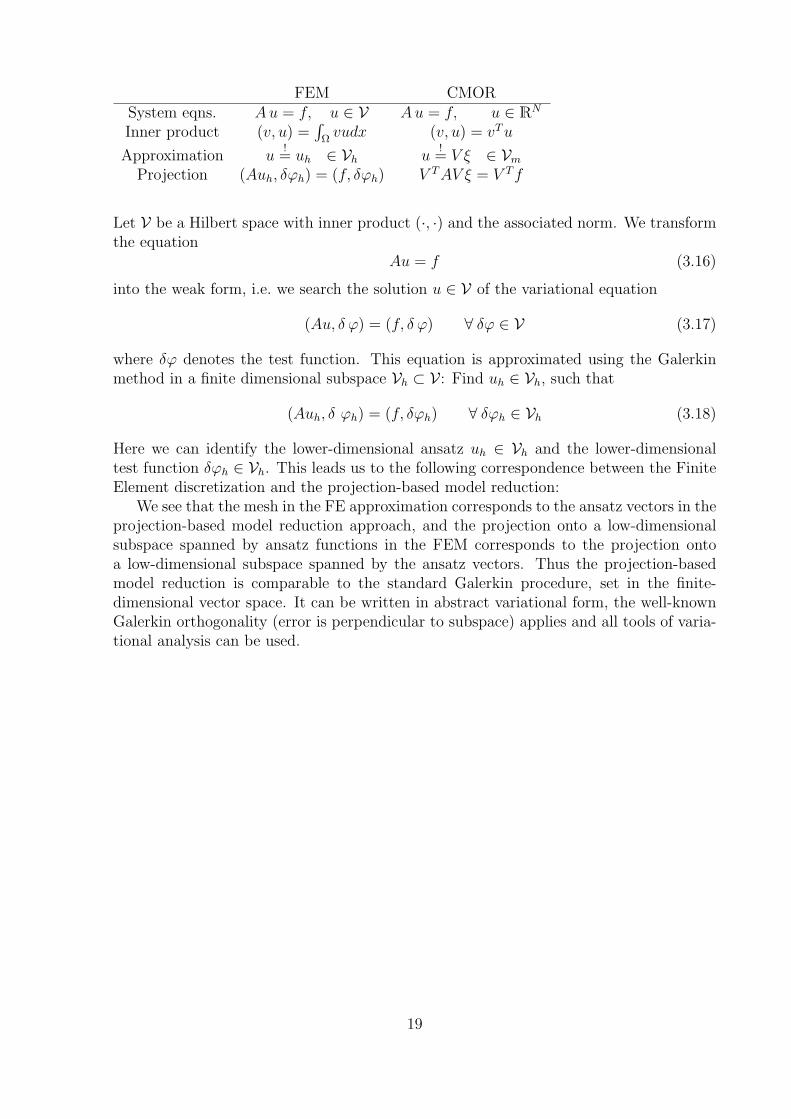
FEM CMORSystem eqns. A u = f, u ∈ V A u = f, u ∈ RN
Inner product (v, u) =∫
Ωvudx (v, u) = vT u
Approximation u!= uh ∈ Vh u
!= V ξ ∈ Vm
Projection (Auh, δϕh) = (f, δϕh) V T AV ξ = V T f
Let V be a Hilbert space with inner product (·, ·) and the associated norm. We transformthe equation
Au = f (3.16)
into the weak form, i.e. we search the solution u ∈ V of the variational equation
(Au, δ ϕ) = (f, δ ϕ) ∀ δϕ ∈ V (3.17)
where δϕ denotes the test function. This equation is approximated using the Galerkinmethod in a finite dimensional subspace Vh ⊂ V: Find uh ∈ Vh, such that
(Auh, δ ϕh) = (f, δϕh) ∀ δϕh ∈ Vh (3.18)
Here we can identify the lower-dimensional ansatz uh ∈ Vh and the lower-dimensionaltest function δϕh ∈ Vh. This leads us to the following correspondence between the FiniteElement discretization and the projection-based model reduction:
We see that the mesh in the FE approximation corresponds to the ansatz vectors in theprojection-based model reduction approach, and the projection onto a low-dimensionalsubspace spanned by ansatz functions in the FEM corresponds to the projection ontoa low-dimensional subspace spanned by the ansatz vectors. Thus the projection-basedmodel reduction is comparable to the standard Galerkin procedure, set in the finite-dimensional vector space. It can be written in abstract variational form, the well-knownGalerkin orthogonality (error is perpendicular to subspace) applies and all tools of varia-tional analysis can be used.
19

3.2 Choices for the basis
The choice of the subspace (and of the basis vectors spanning this subspace) is responsiblefor the quality of the reduced model. Note the difference between basis and subspace:One subspace can be spanned by many different bases, but the choice of basis vectors isresponsible for the numerical behaviour when computing a solution. From the numericalpoint of view it is in general the best choice to use an orthonormal basis for ansatz andtest space, then the resulting system of equations will be well conditioned [16].
In the literature we can find a large number of different bases which have been usedsuccessfully to calculate reduced order systems. For an overview consult Dinkler [15],Noor [56], Leger and Dussault [47]. In the following we will only describe the basesthat are used most frequently.
In the field of linear structural vibrations often the eigenmodes of the structure (alsocalled modes of vibration) are used to form a reduced basis. The method is then calledmodal reduction and, in the case of linear equations, results in a set of decoupled dif-ferential equations. Additionally the physical meaning of the basis vectors leads to theformulation of quantitative criteria for the selection of appropriate basis vectors, for ex-ample based on the comparison of frequency content in the external forcing and theeigenfrequencies of the individual modes of vibration. The first who uses the concept ofmodal reduction for nonlinear systems is Nickell [55]: At each discrete time instant thenonlinear system is linearized and the resulting generalized eigenvalue problem is solved.This repeated solution of an eigenvalue problem leads to a high computational cost, andone can show that frequent changes of the basis can be compared with the introductionof a time-variant constraint, which firstly changes the dynamical behaviour of the systemand secondly leads to numerical problems [34]. The reason for this problematic behaviourlies in the repeated projection of the results of the last time step onto the newly calculatedsubspace.
A second choice for the basis is to use the Lanczos algorithm to generate basis vectors,see for example Nour-Omid and Clough [58] or Wilson et al. [76]. Those Lanczosvectors are the orthonormal vectors that span the Krylov subspace of a certain matrix.The advantage of this approach is that no eigenvalue problem has to be solved. Anotheradvantage in the field of structural dynamics is that this method includes the spatialdistribution of the applied force.
There are several other ideas to extend the bases described above: Almroth et al.[1] propose to use the displacement increment of the first iteration in the solution of thenonlinear system of algebraic equations and Noor and Peters [57] use time derivativesof the solution to enhance the current basis. Noor [56] and Hnle et al. [30] use a mixtureof linear vibrational modes and Lanczos vectors as a basis. Idelson and Cardona [34]use eigenmodes of the linearized equations and also their approximated time derivatives.Chan and Hsiao [10] calculate orthogonalized displacement vectors as the basis for anonlinear static analysis. Chang and Engblom [11] use Lanczos vectors together witha criterium of participation of the individual vectors at a given time instant.
Another basis, which has gained significant attention in the recent history, can befound in the literature under several different names: Karhunen-Loeve expansion [38, 48],principal component analysis [32], empirical orthogonal eigenvectors [51], factor analysis[29], proper orthogonal decomposition (POD)[52] and total least squares [25]. Thereare many applications of this basis, which we call POD basis in the following, in the
20

engineering and scientific sciences, for example in the fields of turbulence research, imageanalysis, or data compression. Additional information can be found in Holmes et al. [31]or Sirovitch and Everson [69]. The POD basis has also proven to be very useful formodel reduction of nonlinear and complex systems: It has been successfully applied tononlinear structural dynamics, fluid dynamics, and fluid-structure interaction problems.By using the POD basis we project the spatio-temporal dynamics on a subspace, in whichthe dominant dynamics takes place. The eigenvectors spanning the POD basis representthe dominant spatial features found in the solution of the dynamical system. Non-typicalfeatures such as noise in the responce are therefore eliminated from the dynamics in thereduced subspace. To use the POD basis we do not need any a-priori information on thesystem under consideration: The POD basis is generated from a given response of thesystem. This can be the solution of the unreduced system (which means we have to beable to solve the original system of equations at least once and for a short amount of time)or a measurement of the real physical system under consideration. The first to use thePOD basis in the field of structural dynamics were Kreuzer and Kust [43], followed byKrysl et al. [44] and Sansour [66]. Especially for nonlinear systems or systems withcomplicated forcing functions, such as random forcing or aeroelastic systems, the PODbasis yields a very efficient basis for the model reduction.
In the following we will take a closer look a the three most important bases for theprojection-based model reduction of dynamical systems, namely the modal basis, theLanczos basis and the POD basis.
3.2.1 Modal basis
To compute the modal basis, we search for a simple linear system of ODEs, for example
Mu + Ku = 0 (3.19)
orAu + Bu = 0, (3.20)
which is in some sene close to our original system. In the case of Mu + Cu + Ku = f wecan for example simply ignore Cu, and in the case of a nonlinear system f(u, u, t) = 0 wehave to calculate the linearization
A =∂f
∂u
∣∣∣∣u0
B =∂f
∂u
∣∣∣∣u0
at a suitable point u0.Then we solve the (generalized) eigenproblem
λ2Mv + Kv = 0
orλAv + Bv = 0 (3.21)
to obtain the eigenvalues λi and eigenvectors vi.
21

In structural dynamics the eigenvectors represent the modes of vibration of the system(or the linearized system at the point u0). The imaginary part of the correspondingeigenvalue describes the frequency of vibration and the real part of the eigenvalue themagnitude of the damping. We then fill the matrix V with some (carefully selected)eigenvectors:
V = [v1, . . . ,vm] . (3.22)
The question concerning the choice of eigenvectors will be answered in the next section.When we substitue the ansatz xm = V mξ, using the eigenvectors of the linear part A,into the original system, for example a nonlinear system in the form
x + Ax + h(x, t) = 0, (3.23)
we obtain for a symmetric matrix A and the normalization of the eigenvectors accordingto vT
i vi = 1 a diagonalization of matrix A,
V TmAV m = diag(αi), (3.24)
and the system reads
ξi + αiξi + hi(V mξ, t) = 0, i = 1 . . . m. (3.25)
Here hi denotes the i-th entry in the vector V Tmh. If the matrix A is non-symmetric, a
diagonalization of the linear part of the equation is only possible when we additionallysolve the adjoint eigenvalue problem [73],
wT A = λw, which is equal to AT w = λw, (3.26)
where wi are called the left eigenvectors, and then we can diagonalize the matrix,
W T AV = diag(αi). (3.27)
But since decoupling of the linear part of the system of equations is not our priority,we always us the same subspace for ansatz and projection. The modal basis is able todescribe the structure’s motion exactly if only the chosen modes v1, . . . , vm are excited bythe external load. There are also some disadvantages of the modal basis:
• Eigenvectors of large matrices are expensive to compute.
• In the case of a nonlinear system
1. a linearization is necessary around u0
2. the eigenvectors are only a good representation of the motion in the vicinityof u0. If the system moves away from u0, the calculated eigenvectors may notdescribe the system behaviour very well and a change of basis vectors might benecessary. But it has been shown that the change of the basis vectors duringtime integration leads to severe numerical problems and thus a change of basisshould be performed as infrequently as possible!
22

Which eigenvectors should be choosen ?
The eigenfrequencies of the eigenvectors can be used as a criterium for the proper se-lection of important eigenvectors for the subspace of the reduced model: We neglectthose eigenvectors with eigenvalues that have a high imaginary part, since these belongto high-frequency vibrations which are firstly non-physical due to the inherent materialdamping and secondly, also very inaccurate due to the comparatively large size of thespatial discretization. In the literature we can find several other criteria, for example
1. Frequency content of the external force: By performing a FFT analysis (Fourieranalysis) of the external forcing function, we get an impression of the frequenciesthat are present in the loading. Then we choose those eigenvectors, which haveeigenfrequencies in the vicinity of the important frequencies of the external force.If the external force has the form
f = f · sin(Ωt), (3.28)
we can calculate the normalized modal amplitudes
ζω,j =1√
(1− η2j )
2·
vTj f√
(vTj vj)(fT f)
where η is the normalized frequency η =
external frequency
Ω
ωj
internal frequency of eigenvector j
2. Calculation of so-called participation factors:
ζx0,j =vT
j Ax0
xT0 Ax0
< ε (3.29)
or
ζv0,j =vT
j Av0
vT0 Av0
< ε (3.30)
where ε describes the desired threshold, matrix A can be M , K, or I, x0 is theinitial deflection and v0 the initial velocity. These participation factors are propermeasures for natural modes vj excited by initial deflection x0 or initial velocitiesv0.
3. When it is important to represent the real mass inertia of the complete model,the efficient mass of the reduced model should nearly equal the total mass. Thiscriterion is important, if free-forced vibrations or vibrations with an activation ofall modes as in case of viscous damping or nonlinearities are considered. The vector
me,j = M · vj
describes the efficient mass of mode vj, that acts in the direction of all unknownsof the complete model. So the normalized efficient mass
%m,j =
√mT
e,jme,j
mtotal
< ε < 1 (3.31)
23

gives an indication which eigenvectors should be chosen. Here mtotal denotes thetotal mass.
3.2.2 Lanczos basis
If it is important to include the steady-state static solution in the reduced basis and ifinner variables like stresses have to be computed accurately by the reduced model, thefollowing basis, called Lanczos basis, is a good choice. It employs the Krylov subspace asthe reduced space: The Krylov subspace Km of dimension m is defined as the subspacespanned by the following vectors
Km = spanv1, Av1, A2v1, . . . A
m−1v1. (3.32)
This subspace is used for the iterative solution of large eigenvalue problems [65], in itera-tive methods for the solution of large linear systems of equations [39], and it can equallywell be used as a basis for model reduction, as shown for example in [76].
This Krylov subspace is a very good subspace for several applications, but the sequenceabove is a very bad basis! Why? The vectors Amv1 will look alike very soon, since it isnot wise numerically to use matrix exponentials. Remember: The subspace defines theapproximation quality in general, whereas the actual basis is responsible for stability androbust numerical behaviour.
To calculate an orthogonal basis, i.e. one with good numerical properties, that spansthe Krylov subspace, one uses the Arnoldi Modified Gram-Schmidt algorithm [65]: As thestarting point we choose an initial vector v1, ||v1|| = 1:
1. Choose v1 with ||v1|| = 1
2. Iterate : For j = 1, 2, ...,m do :
(a) w := Avj
(b) For i = 1, 2, ..., j do
hij = (wivi)
w := w − hijvi
(c) hj+1,j = ‖w‖2(d) vj+1 =
w
hj+1,j
In [65] it is shown that the multiplication of A with V m = v1, . . . ,vm transforms thematrix to upper Hessenberg form,
V TmAV m = Hm. (3.33)
In an Upper-Hessenberg matrix we have hij = 0 for all pairs (i, j) with i > j + 1. Thismeans that we do not obtain a diagonalization of the linear part of the system, even inthe case of a symmetric matrix A, as we obtained when using the modal basis.
In structural dynamics the matrix A is in general formed by the mass matrix M andthe stiffness matrix K,
A = K−1M . (3.34)
The initial vector v1 is chosen to be the static deflection of the system under a represen-tative external load f ext,
v1 = K−1f ext. (3.35)
24

3.2.3 Proper Orthogonal Decomposition
This basis has its roots in the Singular Value Decomposition, i.e. the approximation ofmatrices by means of matrices of lower rank, which are optimal in the 2-norm. Thequestion that arises is whether this result can be applied or extended to the case ofdynamical systems. One straightforward way of applying it to a dynamical system is asfollows: Choose an input function and compute the resulting trajectory. Collect samplesof this trajectory at different times and compute the SVD of the resulting collection ofsamples. This is a method which is widely used in computations involving PDEs, it isknown as the Proper Orthogonal Decomposition (POD). The problem however in thiscase is that the resulting simplification heavily depends on the inital excitation functionchosen, and the time instances at which the measurements are taken. Consequently, thesingular values obtained are not system invariants. The advantage of this method is thatit can be applied to highly complex linear as well as nonlinear systems in a straighforwardmanner. Let us start with a given set of snapshots xi ∈ RN of the system dynamics atdifferent time instants ti:
xi = snapshots of system dynamics of g(x, x, t) = 0 (3.36)
at times ti = t0 + i∆t with i = 0 . . . M . We are looking for a set of orthonormal basisvectors vj, j = 1...N such that
xi =∑
i
αijvj i = 1, ...,M
defines a transformation into the new basis spanned by the vectors vj. This equation isknown as the proper orthogonal decomposition of the family xi. In addition, we requirethat the truncated elements
xk :=k∑
i=1
αijvj reduced basis (since k n) (3.37)
approximate the elements in the family xi optimally, in some average sense. Usuallythis average is defined by means of the autocorrelation matrix
C =1
M
M∑1=1
xixTi . (3.38)
The optimization problem can now be formulated as a matrix approximation prob-lem, namely, find
C :=1
M
M∑i=1
xixTi (3.39)
such that ‖C − C‖2 is minimized.We know that any m×N matrix A can be factored into
A = UΣV T (3.40)
using the Singular Value Decomposition. The column of U are the eigenvectors of AAT
and the column of V are the eigenvectors of AT A. The r singular values on the diag-onal of Σ are the square roots of the nonzero eigenvalues of both AT A and AAT . Forpositive definite matrices this factorization is identical to the eigenvalue decompositionA = QΛQT .
25

3.2.4 The recipe for the POD basis
One way to calculate the POD basis vectors is to perform a SVD of the matrix X =[x1, ...,xM ],
X = [x1, ...,xM ] = UΣV T (3.41)
The first columns of U are the POD basis vectors corresponding to the highest singularvalues. Those are also the eigenvectors of the matrix XXT . But this matrix is a N ×Nmatrix, since x ∈ RN , and if N is very large, it might be prohibitive to use this approach.Here another method can be used, called the Method of Sirovitch, see Sirovitch [68].In this approach we replace the spatial average with the time average, i.e. we replace thecorrelation matrix C with the matrix
B =1
MXT X
which is only M ×M . Note that this change is only valid for ergodic systems. Then thecalculation of the POD vectors is done by performing the following steps:
Method of Sirovitch
1. Calculate or gather snapshots x1, ...,xM
2. Center snapshot ensemble by subtracting the mean value x = 1M
∑Mi xi
xi = xi − x
3. Form the matrix of snapshots
X = [x1|...|xM ]
4. Calculate the temporal covariance matrix of sizeM ×M
B =1
MXT X (3.42)
5. Solve the eigenvalue problemBy = λy
6. Use those eigenvectors yi with the highest eigenvalues λi and calculate the PODbasis vectors according to
vi = Xyi
This means that the POD basis vectors calculated using the method of Sirovitchare linear combinations of the snapshots.
Two other remarks concerning the POD basis:
• Remark 1 : It is often stated to first center the point cloud [x1, ...,xM ]by subtracting the mean x = 1
M
∑xi
X = [x1 − x, ...,xM − x]
26
and use the ansatz
x ≈ xm = x + V ξi
where vi are POD vectors of X. But if you do not center the snapshots, the firstPOD vector will be the mean x.
• Remark 2 : If you have collected variables with very different physical meaning inx (for example pressure and velocity) it is better to normalize the snapshots usingthe standard deviation vector
s =
√√√√ 1
M − 1
M∑i=1
(xi − x)2 = std(X) (3.43)
The normalised snapshots are then given by
X = X./s (3.44)
calculated by element-wise division.
3.3 Problems
1. Write an m-function
[V] = modalBasis(M,K,m)
that calculates the m eigenvectors of the generalized eigenvalue problem
λ2Mv + Kv = λv (3.45)
with the lowest eigenfrequencies and returns the matrix V = [v1, . . . ,vm].
2. Write an m-function
[V] = lanczosBasis(A,v1,m)
that calculates the first m vectors of the Krylov subspace
Km = spany1, Av1, A2v1, . . . A
m−1v1. (3.46)
using the Arnoldi Modified Gram-Schmidt algorithm and returns the matrix V =[v1, . . . ,vm].
3. Write an m-function
27

[V] = podBasisSVD(X,m)
that calculates the m first vectors vi of the POD basis of the snapshots in matrixX, employing the SVD of X, and returns the matrix V = [v1, . . . ,vm].
4. Write an m-function
[V] = podBasisSIR(X,m)
that calculates the m first vectors vi of the POD basis of the snapshots in matrixX, employing the method of Sirovitch, and returns the matrix V = [v1, . . . ,vm].
5. Download the linear FEM solver
linearFEM.tgz
and extract it into a subdirectory.
(a) Use the provided mass and stiffness matrices to calculate the first m modalbasis vectors with the lowest eigenfrequencies.
(b) Use the external force together with the mass and stiffness matrices to calculatethe first m Lanczos basis vectors.
(c) Solve the system for the first 2 seconds and save the snapshots at ∆t = 0.2 sec.Calculate the POD basis (SVD) and the POD basis (Sirovitch) using m=10.
(d) Display the first and second basis vectors of each basis. What are the differ-ences?
28

Chapter 4Time discretization of the reduced model
After the spatial discretization of the PDE we have to perform the temporal discretizationof the resulting system of ODEs to obtain the solution. In general we have two possibilitiesto integrate a system of ODEs in time:
1. Explicit methods, and
2. Implicit methods.
Using an explicit method has the following advantages and disadvantages:
+ If the system of ODEs is given in explicit form,
x = f(x, t)
we do not have to solve any system of algebraic equations during the integration intime, even if the problem is nonlinear.
– The maximal time step size for a stable integration is restricted by the highest fre-quency that occurs in the system. This criterium can severely limit the stepsize andneccessitate many small time steps, which would not be needed from the accuracypoint-of-view.
Using an implicit method has the following advantages and disadvantages
+ The time step size for a stable integration is not restricted by the highest frequencyin the system, it is only determined by the accuracy needed for the solution.
– In every time step we have to solve a linear or nonlinear system of algearic equations(AEs). This can be very costly, if the dimension of the system of ODEs is large.
For both explicit and implicit time discretization methods the model reduction yieldsbenefits:
1. When using explicit methods, the stable time step length will often increase signif-icantly for the reduced model, since the highest frequencies, which limit the stabletime step and are often only present due to the fine spatial discretization, are notpresent in the reduced model, as shown for example in Bucher [7].
2. When using an implicit time discretization, the size of the system of linear or non-linear equations that has to be solved in each time step is reduced significantly, seefor example Krysl et al. [44] or Remke and Rothert [62] for an evaluation of theefficiency gain when using reduced models.
29
4.1 Explicit Euler Time Integration
Let us start with the simplest possible setup to explain the differences between the timeintegration of original and reduced model: To solve the linear system
x = g(x, t) = Ax + f(t) (4.1)
x(t = 0) = x0.
in time, we use the Explit Euler time integration, given by
xn+1 = xn + ∆t g(xn, tn). (4.2)
This yieldsxn+1 = xn + ∆tAxn + ∆tf(tn) (4.3)
for the original system. Now we use the Ansatz x = V ξ, substitute and project to obtainthe reduced system
V T V ξ = V T g(V ξ, t) = V T AV ξ + V T f(t) (4.4)
In addition we have to project the initial conditions onto the subspace:
V T V ξ(t = 0) = V T x0 (4.5)
which yieldsξ(t = 0) = (V T V )−1V T x0. (4.6)
The reduced system that we have to solve in time now reads as follows, assuming that Vis orthonormal, i.e. V T V = I,
ξn+1 = ξn + ∆tV T AV ξn + ∆tV T f(tn). (4.7)
This means that we have to calculate the reduced matrix Ared = V T AV once at thebeginning together with ξ(t = 0) and, during the integration, project the external forcingfunction f onto the subspace at each time step. This clearly shows that the quality of thereduced model compared to the original model will be better if the projection fm = V T fcaptures as much of the original vector f as possible. The benefit of using the reducedmodel lies in the increase of the stable time step length, we need less steps than whenintegrating the original system.
4.2 Implicit Euler Time Integration
As a second example, let us apply the Implicit Euler method
xn+1 = xn + ∆tg(xn+1, tn+1) (4.8)
to the system above. For the original system this yields
xn+1 = xn + ∆t (Axn+1 + f(tn+1)) (4.9)
30

which we have to solve for xn+1:
(I −∆tA)xn+1 = xn + ∆tf(tn+1) (4.10)
xn+1 = (I −∆tA)−1 (xn + ∆tf(tn+1)) . (4.11)
Applying the Implict Euler method to the reduced order model, we obtain
ξn+1 = ξn + ∆t(V T AV ξn+1 + V T f(tn+1)
)(4.12)
ξn+1 = (I −∆tV T AV )−1(ξn + ∆tV T f(tn+1)
). (4.13)
If you compare eq. (4.11) with eq. (4.13), you see that instead of having to solve a systemof dimension N , we only have to solve a system of dimension m (since x ∈ RN , ξ ∈ RM)when integrating the reduced system. This will typically be done by LU decomposition atthe beginning (and whenever the time step changes) and one forward and one backwardsubstitution in each time step.
4.3 Newmark method for 2nd order systems
As a final example let us consider the time integration of a nonlinear system of ODEsof 2nd order, which often arises in the field of structural dynamics, by employing theNewmark method. At time instant tn+1 the following system of ODEs has to be satisfied:
F (an+1, vn+1, dn+1, tn+1) = 0. (4.14)
Here dn+1, vn+1,and an+1 are the approximations of d, d and d at time tn+1. Those arethe vectors of displacements, velocities and accelerations, respectively. The values of dn,vn and an of the previous time instant are known. We need two additional equations tobe able to solve this system. Those are the Newmark equations
dn+1 = dn + dt vn +dt2
2[(1− 2β)an+1 + 2βan] , (4.15)
vn+1 = vn + dt [(1− γ)an + γan+1] . (4.16)
If we choose γ = 12
and β = 14, we obtain the so-called trapezoidal rule. This method has
second order accuracy and is A-stable for linear systems.If we solve the Newmark equations for an+1 and vn+1, and substitute those into the
equations of motion F , we obtain a nonlinear system of equations in the variables dn+1.This nonlinear system is often solved with the Newton method or a variant of it likeQuasi-Newton, etc. [63, 39]. We will employ the standard Newton method for solving thenonlinear system g(x) = 0. We first write the Taylor series expansion of g(x) at the pointx0,
g(x) = g(x0) + J(x0)(x− x0) + · · · (4.17)
with the Jacobian matrix
J(x0) =∂g
∂x
∣∣∣∣x0
(4.18)
and ignore terms of higher order.
g(x) = 0 = g(x0) + J(x0) ·∆x (4.19)
31

where ∆x = (x− x0). Then we solve the remaining system for x
∆x = −J−1(x0) · g(x0) (4.20)
x = x + ∆x. (4.21)
(4.22)
Since we ignored the terms of higher order, we have to iterate this to obtain the solutionto the nonlinear system of equations.
We finally get the following algorithm for the time integration of nonlinear systems ofsecond order with the Newmark method:
i← 0
d(i)n+1 = dn
a(i)n+1 = − 1
βdtvn +
(1− 1
2β
)an
v(i)n+1 = vn + dt
[(1− γ)an + γa
(i)n+1
] predictor=initial guess
Iterate : i← i + 1
K(i)eff = 1
βdt2M + γ
βdtC + K effective stiffness matrix
%(i) = F (a(i)n+1, v
(i)n+1, d
(i)n+1, tn+1) residual
∆d(i) = −(K(i)eff )
−1%(i) displacement increment
d(i)n+1 = d(i−1)
n + ∆d(i)
v(i)n+1 = v
(i−1)n + γ
βdt∆d(i)
a(i)n+1 = a
(i−1)n + 1
βdt2∆d(i)
corrector
If ||%(i)|| > ε||%(0)|| repeat iteration,else set t← t + dt and start from above.
(4.23)
Here Keff is the Jakobian of the system, which is often called effective stiffness matrixin the structural dynamics literature,
Keff =∂F
∂an+1
∂an+1
∂dn+1
+∂F
∂vn+1
∂vn+1
∂dn+1
+∂F
∂dn+1
= M1
βh2+ C
γ
βh+ K (4.24)
with the matrices
M =∂F
∂an+1
(4.25)
C =∂F
∂vn+1
(4.26)
K =∂F
∂dn+1
. (4.27)
32

Now we apply the Newmark method to the reduced order model. Here the integrationalgorithm reads:
i← 0
d(i)n+1 = dn
a(i)n+1 = − 1
βdtvn +
(1− 1
2β
)an
v(i)n+1 = vn + dt
[(1− γ)an + γa
(i)n+1
] predictor
Iterate : i← i + 1
K(i)eff,red = 1
βdt2M red + γ
βdtCred + Kred reduced effective stiffness matrix
%(i)red = V T F (a
(i)n+1, v
(i)n+1, d
(i)n+1, tn+1) reduced residual
∆ξ(i) = −(K(i)eff,red)
−1%(i)red reduced displacement increment
∆d(i) = V ∆ξ(i) displacement increment
d(i)n+1 = d(i−1)
n + ∆d(i)
v(i)n+1 = v
(i−1)n + γ
βdt∆d(i)
a(i)n+1 = a
(i−1)n + 1
βdt2∆d(i)
corrector
If ||%(i)red|| > ε||%(0)
red|| repeat iteration,else set t← t + dt and start from above.
(4.28)
The reduced stiffness matrix above includes the terms
M red = V T ∂F
∂an+1
V (4.29)
Cred = V T ∂F
∂vn+1
V (4.30)
Kred = V T ∂F
∂dn+1
V . (4.31)
Also we have to project the initial conditions for displacement and velocity onto thesubspace of the reduced model:
d0,red = (V T V )−1V T d0, (4.32)
v0,red = (V T V )−1V T v0. (4.33)
If we compare the algorithms for original and reduced system, we see surprisingly fewdifferences. We only assemble the reduced stiffness matrix instead of the original oneand project the residual onto the chosen subspace. Then we solve for the intermediatevariables ξ, but immediately change back to the original variables d = V ξ. Since westart with initial conditions that have been projected onto the subspace and during thetime integration only add components that also lie on this subspace, we can be sure thatalthough we keep using the original variables, they do not drift away from the subspace ofthe reduced model. Note that we can not reduce once at the beginning as it was the casewith the linear system. We have to keep evaluating the residual of the full, unreduced
33

system and project this afterwards. The only benefit of using the reduced model is themuch smaller size of the reduced effective stiffness matrix, which is only m×m, if ξ ∈ Rm
instead of N × N , when d ∈ RN . Thus, if the computational cost of evaluating theresidual is low in comparison to solving the large system of equations, it is beneficial touse reduced order models to speed up the integration in the case of nonlinear systems.
4.4 cG(q) time discretization
We can also use the finite element approach for the time discretization of the systemsof ODEs. The resulting methods are sometimes called variational integrators. A goodoverview on this approach can be found in Eriksson et al. [16]. The name cG(q) tellsus that we use the continuous Galerkin method with the order q. This means thatthe temporal behaviour of the variabls is approximated with continuous functions thathave derivatives of up to the order q. In contrast to the cG(q) method the dG(q) usesdiscontinuous functions that can have jumps at a certain point in time tn. (Those tn arethe boundaries of the time finite elements.)
To derive the cG(q) method, we write the system of 1st order
x + g(x, t) = 0, 0 < t ≤ T,
x(0) = x0, x ∈ Rd. (4.34)
in variational (weak) form: We search for the vector-valued funktion x ∈ C(q)([0, T ]), sothat ∫ T
0
〈x + g(x(t), t), δϕ(t)〉dt = 0, x(0) = x0, ∀ δϕ ∈ C(q)([0, T ]), (4.35)
where C(q)([0, T ]) denotes the set of all functions with continuous derivatives up to theorder q on [0, T ]. Now we construct a piecewise polynomial approximation xk for x bysubdividing the interval [0, T ] into
0 := t0 < t1 < · · · < tN := T (4.36)
We define the time step sizes ∆tn := tn − tn−1 and the time intervals In := [tn−1, tn].Ansatz space for the finite time elements is the space C(q) = C(q)([0, T ]), i.e. the space ofcontinuous polynomials of order q on each interval In,
C(q) :=U ∈ C0([0, T ]) : U |In ∈ P(q)(In), 1 ≤ n ≤ N
. (4.37)
Here P(q)(In) denotes the polynomials in Rd with order q in In. Since we want continuityfrom time interval to time interval, a function in C(q) has only q degrees of freedom ineach interval. As test space we use
D(q−1) = D(q−1)([0, T ]) :=U : U |In ∈ P(q−1)(In), 1 ≤ n ≤ N
. (4.38)
Those functions are not necessarily continuous: U+,−n denotes the left (resp. right) limit
of U ∈ D(q−1) at time tn and [U ]n := U+n − U−
n denotes the jump at tn. For 1 ≤ n ≤ Nthe cG(q) method calculates the approximation xk ∈ C(q) of the equation
n∑n=1
∫In
〈xk + g(xk, t), δϕk〉dt = 0, xk(0) = x0, ∀ δϕk ∈ D(q−1). (4.39)
34

If q = 1, then xk is the piecewise linear function
xk|In= xk,n−1
(t− tn)
−∆tn+ xk,n
(t− tn−1)
∆tn, (4.40)
where the coefficient xk,n is the solution of the equation
xk,n +
∫In
g(xk(t), t)dt = xk,n−1. (4.41)
If we use the trapezoidal rule to calculate the value of this integral,∫In
g(xk(t), t) dt ≈ ∆tn2
[g(xk,n−1, tn−1) + g(xk,n, tn)] , (4.42)
we recover the classical trapezoidal method for 1st order ODE systems, which is the sameas the Newmark method for second order systems if β = 1/4 and γ = 1/2, see also [2].Thus those two methods are variational methods - they can be written in variational formand all tools of variational analysis apply.
35

Chapter 5Improving the accuracy of the reduced model
One obvious choice to improve the accuracy of the reduced model is to use more basisvectors in the reduced basis. But there are also other, more elaborate methods to obtaina reduced model with a higher accuracy: In this chapter we will present three methodsthat can be employed to improve the approximation quality of the reduced model:
(a) The static correction method [28, 33], also called mode acceleration method, forlinear systems, and the
(b) Nonlinear Galerkin method [54, 14, 46] and
(c) Postprocessed Galerkin method [23, 45], both applicable to nonlinear systems.
5.1 Static Correction Method
When comparing the solution of reduced and unreduced model for linear structural vi-brations, often the dynamics of the system are well captured by the reduced system. Butderived quantities like inner forces and moments often are not approximated very well[40]. The static correction method tries to alleviate this shortcoming.
If the spatial distribution of the forcing function is such that the higher modes aresignificantly excited, these modes must be included in the analysis. At the same time, ifthe frequency of the eigenmodes is much larger than the highest frequency content of theexternal loading, the response in the higher-frequency modes is essentially static. Thus,if we include all available modes in the analysis, but assume that for the modes v[m+1,...,n]
the response is static, we can come up with a method to improve the accuracy of thesolution of the reduced model, called the static correction method: We want to reducethe following linear system,
Mu + Ku = ff(t) (5.1)
where the forcing function can be decomposed into a spatial part, given by the vector fand a scalar temporal part f(t). As usual we calculate the eigenmodes of the generalizedeigenvalue problem to obtain the modal ansatz vectors for the model reduction. Now weput the first m eigenvectors with the lowest frequencies in V = [v1, . . . ,vm] and use theansatz
u ≈ V ξ. (5.2)
36

The trick of the static correction method now is to improve the ansatz above with anotherterm:
u ≈ V ξ + urest · f(t) (5.3)
This means that only the modes in V contribute dynamically, every other mode which weignored previously, i.e. [vm+1, . . . ,vn] contributes only statically with the time functiongiven by the forcing f(t). In other words: The structure follows the load f ·f(t) statically inthe subspace spanned by the modes [vm+1, . . . ,vn]. Now we have to answer the question:What exactly is urest? To calculate this quantity, let us first calculate the static solutionustat, which is given by
ustat = K−1 · f (5.4)
Now we have to take into account that a part of the static solution ustat is already includedin the term V ξ, i.e.
um,stat = V (V T KV )−1V T ff(t), (5.5)
thus we have the relationship
urest = ustat − um,stat. (5.6)
This leads to the final equation
u ≈ V ξ + [ustat − um,rest] (5.7)
≈ V ξ +[K−1 f − V (V T KV )−1V T f
]· f(t) (5.8)
where ξ is the solution of the reduced model
V T MV ξ + V T KV ξ = V T ff(t) (5.9)
In this derivation we have assumed a special form of the external loading,
f = f · f(t) (5.10)
If this is not the case, we can still use the same idea. We start with
Mu + Ku = f(t), (5.11)
where the right hand side f(t) does not have any special form, and solve again for theeigenvectors. Then we use an extended ansatz
um =[
V W]·[ξη
]= V ξ︸︷︷︸
old ansatz
+ Wη︸︷︷︸new part
(5.12)
This means that we calculate some more eigenmodes and put those into the matrix W .The matrix V is the same as above. Now we substitute and project twice:
1. firstly on the space spanned by the vectors in V , and
2. secondly on the space spanned by the vectors in W .
37

As result we get the following two systems
V T M(V ξ + Wη) + V T K(V ξ + W η) = V T f (5.13)
W T M(V ξ + Wη) + W T K(V ξ + Wη) = W T f (5.14)
If we take a closer look at the two systems above, we can simplify them considerably,because all vi are M and K orthogonal to the vectors wj. This means that we have
V T MW = 0 V T KW = 0 (5.15)
W T MV = 0 W T KV = 0. (5.16)
Finally we arrive at the following two systems of equations,
V T MV ξ + V T KV ξ = V T f (5.17)
W T MWη + W T KWη = W T f (5.18)
Now we make the assumption of the static correction method, that η ≡ 0. This meansthat the second system behaves quasi-static, i.e. it follows the load W T f immediatelywithout inertia effects. This leaves us with the following two systems:
V T MV ξ + V T KV ξ = V T f (5.19)
W T KWη = W T f (5.20)
Now we solve the system given by eq. (5.19) in time as before. In every time step whereoutput is needed, we also solve eq. (5.20) and improve the solution using the static cor-rection Wη:
uimproved = V ξ + Wη (5.21)
5.2 Nonlinear and Postprocessed Galerkin method
The static correction method described in the previous section is only applicable to linearsystems. Now the questions arises: Can we extend the idea of the static correction methodto nonlinear systems? The answer is yes and the resulting numerical methods are calledthe Nonlinear Galerkin method and the Postprocessed Galerkin method: The projection-based model reduction, which we have decribed in the previous chapters, projects theoriginal equations onto a linear, i.e. flat subspace - thus this method is also known asthe flat Galerkin method. Nonlinear extensions of the flat Galerkin method, thereforecalled Nonlinear Galerkin methods [54, 14, 46], rely on the assumption that the long-termdynamics of dissipative dynamical systems will converge to a low-dimensional subspace[71], the so-called attractor. If we want to describe the long-term dynamic behaviourefficiently, we have to approximate this attractor, which is hopefully living in a small-dimensional subspace. The underlying theory for this approach is based on the InertialManifold Theory (IM) [22, 71], which is a global extension of the (local) Center ManifoldTheory (CM) [9]. Before we describe the nonlinear Galerkin method, we repeat theconcepts of invariant manifolds and the center manifold theory. A good introduction to thetheory of nonlinear dynamical systems can be found in Wiggins [75], Guckenheimerand Holmes [26] and Temam [71].
38

5.2.1 Invariant manifolds
Invariant manifolds, especially the stable, instable and center manifolds, play an impor-tant role in the analysis of dynamical systems. Let us consider the following nonlineardynamical system: x∗ ∈ RN is a fixed point of
x = g(x). (5.22)
For a local stability analysis we have to analyse the linear system
w = Aw, A =∂g
∂x
∣∣∣∣x∗
, w = x− x∗. (5.23)
The solution of this linear system with the initial conditions w(0) = w0 is given by
w(t) = eAtw0. (5.24)
A very useful basis for this solution is spanned by the eigenvectors of the matrix A. Thisspace can be separated into three subspaces:
RN = Es × Eu × Ec. (5.25)
Here
• Es is spanned by the eigenvectors of A that belong to those eigevalues with a negativereal part, called stable manifold with dimension ds,
• Eu is spanned by the eigenvectors of A that belong to those eigevalues with a positivereal part, called instable manifold with dimension du, and
• Ec is spanned by the eigenvectors of A that belong to those eigevalues with a zeroreal part, called center manifold with dimension dc.
The dimensions of the three subspaces sum up to N , N = ds + du + dc. Es, Eu und Ec
are called the invariant subspaces of the linear dynamical system, because solutions of eq.(5.23), whose initial conditions lie completely in one of these invariant subspaces, stay inthis subspace forever. Also for nonlinear systems like eq. (5.22) there exist stable, instableand center manifolds. Those are nonlinear subspaces, which we can locally describe inRN .
Back to our stability analysis - we wanted to know the stability of solutions of thenonlinear system (5.22) close to the fixed point. Let us translate the system into the fixedpoint,
w = x− x∗ (5.26)
and perform a Taylor expansion around x∗. Then we obtain the following system fromeq. (5.22):
w = Aw + h(w), (5.27)
where h(w) = O(||w||2). Now we transform matrix A to diagonal form:
Aw =
As 0 00 Au 00 0 Ac
ws
wu
wc
, (5.28)
39

where X−1w ≡ (wTs , wT
u , wTc )T ∈ Rds ×Rdu ×Rdc defines the transformation. Here As is
a ds× ds matrix with eigenvalues with negative real parts, Au is a du× du matrix, whoseeigenvalues have positive real parts, and Ac is a dc×dc matrix with eigenvalues with zeroreal part. This leads us to the following three coupled systems of equations, called thenormal form of eq. (5.22):
ws = Asws + hs(ws, wu, wc),
wu = Auwu + hu(ws, wu, wc), (5.29)
wc = Acwc + hc(us, wu, wc),
where hs (hu, hc) denotes the first ds (du, dc) components of the vector X−1h(w) .
5.2.2 The center manifold
If the instable manifold is empty, every trajectory that lives in the subspace Es will beattracted by the center manifold in an exponential rate - its components in the stablemanifold decay exponentially. This leads us to the conclusion that for the analysis of thelong-term behaviour of the system it is sufficient to look at the dynamics of the systemrestricted to the center manifold. The main application area of the center manifold theory,see for example Carr [9], is the bifurcation analysis of nonlinear dynamical systems. Butit can also be used for the dimension reduction of dynamical systems, if some assumptionshold true. Let us consider the following system in normal form:
ws = Asws + hs(ws, wc)
wc = Acwc + hc(ws, wc), (ws, wc) ∈ Rds × Rdc , (5.30)
where hs and hc as well as their derivatives at zero have to be zero. In Carr [9] wefind the proof that if those assumptions hold true, the system (5.30) has a local centermanifold of the form
ws = Φ(wc) fr ||ws|| < ε. (5.31)
Geometrically this is a (often nonlinear) hyper-surface in the space Ec×Es, which is givenby the function Φ(wc) = ws. The reduction principle of the center manifold theory tellsus that the asymptotic (i.e. long-term) dynamics of the original system is confined to thecenter manifold. Thus we have
wc = Acwc + hc(wc,Φ(wc)), wc ∈ Rdc . (5.32)
A proof can be found in [9]. This system now has only the dimension dc and describesthe long-term behaviour of (5.30). The center manifold theory can also be applied tonon-autonomous systems and PDEs. A detailed description of the procedure to calculatethe function Φ and several examples can be found in [9].
5.2.3 Inertial manifolds and the nonlinear Galerkin method
The inertial manifold can be seen as the global analogon of the center manifold of theprevious section for dissipative ODEs or PDEs [12]. A set M is an inertial manifold, ifthe following points are true:
40
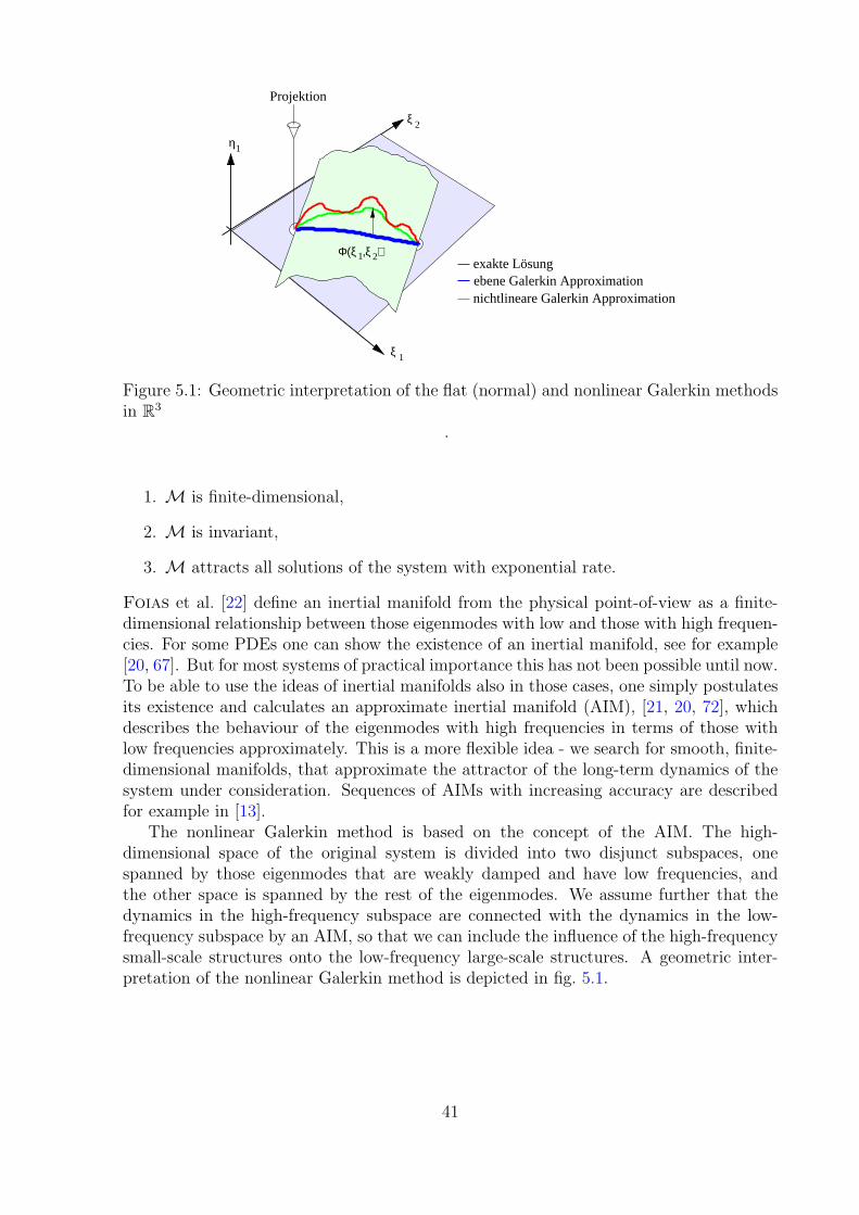
Projektion
ξ 1
ξ 2
1
nichtlineare Galerkin Approximationebene Galerkin Approximationexakte Lösung
η
2Φ(ξ ,ξ )1
Figure 5.1: Geometric interpretation of the flat (normal) and nonlinear Galerkin methodsin R3
.
1. M is finite-dimensional,
2. M is invariant,
3. M attracts all solutions of the system with exponential rate.
Foias et al. [22] define an inertial manifold from the physical point-of-view as a finite-dimensional relationship between those eigenmodes with low and those with high frequen-cies. For some PDEs one can show the existence of an inertial manifold, see for example[20, 67]. But for most systems of practical importance this has not been possible until now.To be able to use the ideas of inertial manifolds also in those cases, one simply postulatesits existence and calculates an approximate inertial manifold (AIM), [21, 20, 72], whichdescribes the behaviour of the eigenmodes with high frequencies in terms of those withlow frequencies approximately. This is a more flexible idea - we search for smooth, finite-dimensional manifolds, that approximate the attractor of the long-term dynamics of thesystem under consideration. Sequences of AIMs with increasing accuracy are describedfor example in [13].
The nonlinear Galerkin method is based on the concept of the AIM. The high-dimensional space of the original system is divided into two disjunct subspaces, onespanned by those eigenmodes that are weakly damped and have low frequencies, andthe other space is spanned by the rest of the eigenmodes. We assume further that thedynamics in the high-frequency subspace are connected with the dynamics in the low-frequency subspace by an AIM, so that we can include the influence of the high-frequencysmall-scale structures onto the low-frequency large-scale structures. A geometric inter-pretation of the nonlinear Galerkin method is depicted in fig. 5.1.
41

5.2.4 The nonlinear Galerkin method
Let us descibe the nonlinear Galerkin method applied to a nonlinear system of first order,
x + Ax + h(x, t) = 0, x ∈ RN (5.33)
where Ax is the linear and h the nonlinear part. We calculate the eigenvectors y of thematrix A,
Ayj = λjyj. (5.34)
The first m eigenvectors, sorted by frequency and damping - remember, we want thelow-frequency and little-damped eigenmodes - are put into the matrix Y m. These vec-tors span the m-dimensional subspace Ym = spany1, . . . ,ym. Into the matrix ZN−m
we put the rest of the eigenvectors, those span the complementary subspace Zd−m =spanym+1, . . . ,yd to the subspace Ym. Let the eigenvectors also be orthonormal, sothat we have yT
i yj = δij. Since Rd = Ym ×Zm, the following equation is not an approxi-mation, but a transformation into another basis:
x = Y mξ + ZN−mη. (5.35)
We substitute eq. (5.35) into eq. (5.33) and project by multiplication with Y Tm and ZT
d−m
from the left onto the mutually orthogonal subspaces Ym and Zd−m, we obtain the twocoupled systems of ODEs,
ξ + Y TmAY mξ + Y T
mh(Y mξ + ZN−mη, t) = 0, (5.36)
η + ZTN−mAZN−mη + ZT
d−mh(Y mξ + ZN−mη, t) = 0. (5.37)
The flat Galerkin method now sets η = 0 in eq. (5.36) and integrates the resulting finite-dimensional system
ξ + Y TmAY ξ + Y T
mh(Y mξ, t) = 0 (5.38)
in time. The true solution of eq. (5.33) is approximated by x ≈ Y mξ.Under the assumption that the atrractor of eq. (5.33) can be described by a small
number of variables, it is a good idea to postulate that for a certain value of m and thecorrect separation of the basis vectors into Y m and ZN−m there exists a relationshipbetween ξ and η, so that we have
η = Φ(ξ) (5.39)
on the attractor. Physically this means that on the attractor of the system the behaviourof all high-frequency highly-damped eigenmodes is governed by the behaviour of the low-frequency little-damped eigenmodes. In the field of Synergetics, see for example Haken[27], this characteristic of the system is called the enslavement-principle. By substitutingeq. (5.39) into eq. (5.36) and integrating the resulting m-dimensional system
ξ + Y TmAY mξ + Y T
mh(Y mξ + ZN−mΦ(ξ), t) = 0 (5.40)
in time, we can reconstruct the solution x = Y mξ + ZN−mΦ(ξ) without any approxima-tion error, although we only solve a system of degree m instead of N .
Since one cannot prove the existence of an inertial manifold for most systems of prac-tical importance, we instead postulate the existence of an approximate inertial manifold
42

Φapp. This function shall approximate the behaviour of the high-frequency modes bythose with low frequencies. Then we integrate the equation
ξ + Y TmAY mξ + Y T
mh(Y mξ + ZN−mΦapp(ξ), t) = 0 (5.41)
in time and the solution is approximated as x ≈ Y mξ + ZN−mΦapp(ξ). This approxima-tion will not describe the system dynamics on the attractor exactly, but we hope that theaccuracy of the solution is better that the solution without using the AIM relationship,i.e. the solution of the flat Galerkin method.
5.2.5 Postprocessed Galerkin method
One drawback may be the computational cost of calculating Φapp, and if this computa-tional cost is not small, it might be better to use the flat Galerkin method with more basisvectors m > m instead of solving eq. (5.41). Here the postprocessed Galerkin Method ofGarcıa-Archilla et al. [23] comes into play: They show that often we can reach theaccuracy of the system given by eq. (5.41), but only with a computational cost that iscomparable to the cost of the traditional m-dimensional Galerkin projection. The idea ofthe postprocessed Galerkin method is to integrate eq. (5.38) in time, and to calculate theAIM only at those instants in time where output values are needed. In other words: Atoutput time instants we lift the solution of the flat Galerkin method onto the approximateinertial manifold:
x(tn) ≈ Y mξ(tn) + ZN−mΦapp(ξ(tn)). (5.42)
This approach has been shown to be successful when applied to certain structural dy-namics problems, see for example Laing et al. [45], where the postprocessed Galerkinmethod has a similar accuracy as the nonlinear Galerkin method, but a computationalcost comparable to the flat Galerkin method,
5.2.6 Approximate inertial manifolds
Finally we have to answer the question of how to calculate an AIM Φapp. A nice overviewcan be found in Russel et al. [64]: Starting from eq. (5.37) we try to find an approxi-mation for the relationship η = Φapp(ξ). This means we have to solve the equation
η + ZTN−mAZN−mη + ZT
N−mh(Y mξ + ZN−mη, t) = 0 (5.43)
in time. This could be done for example using simple methods of low order: The so-calledEuler-Galerkin AIM [20] uses the implicit Euler discretization. Using the time step τ andthe initial condition η = 0 we get the following relationship,
η = Φapp(ξ) = −τ(I + τZTN−mAZN−m)−1ZT
N−mh(Y mξ, t). (5.44)
where we have used one fixed-point iteration to solve the nonlinear system of equations.The question on how to choose the size of τ is difficult to answer. Using a small value willyield a high accuracy, but only if η = 0 is a good initial guess for the solution. The choiceτ ≈ 1/λm+1, i.e. proportional to the reciprocal value of the first neglected eigenvalue, isrecommended in [20].
Another approach to arrive at the AIM is shown in Titi [72] and can be seen as thestatic correction approach applied to nonlinear systems. We make the assumption that
43

the time derivative η can be neglected and calculate a quasi-stationary AIM. This meansthat the variables η follow the variables ξ without inertia effects. Then we have to solvethe algebraic equation
g(η) := ZTN−mAZN−mη + ZT
N−mh(Y mξ + ZN−mη, t) = 0 (5.45)
Thus we replace the system given by eqns. (5.36,5.37) of ODEs by a system of differential-algebraic equations (DAEs), given by eqns. (5.36,5.45). Often the algebraic system issolved with fixed-point iteration and one or two iteration cycles. As alternative we canalso use the Newton-Raphson method. But since the computational cost to evaluate Φapp
should be as small as possible, often the fixed-point iteration is used in applications [45].For the initial guess of the iterative solution of the nonlinear system we can choose eitherη = 0 or the value of η of the last time step.
5.2.7 Nonlinear Galerkin method and Newmark time integra-tion
Here we need an easier example.To summarize, the Newmark algorithm with the nonlinear Galerkin method reads as
follows:
Set iteration counter i = 0, calculate initial guess d(i)n+1, v
(i)n+1, a
(i)n+1
Calculate residual ρ(i)
redStart iteration, i = i + 1
Evaluate AIM(d(i−1)n+1 , v
(i−1)n+1 , a
(i−1)n+1 )
Calculate correction d(i−1)n+1 = d
(i−1)n+1 +AIM
Calculate residual ρ(i−1)
red and K(i−1)
eff,red
Solve ∆d(i) = −Y Tm(K
(i−1)
eff,red)−1ρ(i−1)
redUpdate variables d
(i)n+1, v
(i)n+1, a
(i)n+1
Calculate ρ(i)
redIf ||ρ(i)
red|| ≤ ε||ρ(0)
red|| → end iterationStart next time step.
In grey we have the changes to the normal Galerkin method: Since we use the AIMwe need an additional evaluation of the residual per iteration. This might lead to anunacceptable increase in computing time, if this residual evaluation is costly.
Let us therefore consider the Postprocessed Galerkin method with the quasi-staticAIM:
Set i = 0, calculate initial guesses d(i)n+1, v
(i)n+1, a
(i)n+1
Calculate ρ(i)
red and K(i)
eff,redStart iteration, i = i + 1
Solve ∆d(i) = −Y Tm(K
(i−1)
eff,red)−1ρ(i−1)
redUpdate variables d
(i)n+1, v
(i)n+1, a
(i)n+1
Calculate ρ(i)
red und K(i)
eff,redIf ||ρ(i)
red|| ≤ ε||ρ(0)
red|| → end iteration
44

Evaluate AIM(d(i)n+1, v
(i)n+1, a
(i)n+1)
Calculate d(i)
n+1 = d(i)n+1+AIM
Start next time step.
The additional calculations involve only on matrix-vector multiplication, which we haveto do at most once per time step.
45

Chapter 6Error Estimation
Approximation, like all modeling, in general leads to the classical dilemma: Accuracyor simplicity? The engineer has to evaluate how important accuracy is compared tosimplicity. Indeed, it is very important to know the measure of the error introduced inthe approximation for a fixed set of signals, and it is therefore important to establishsome criteria of approximation in such a way as to give some guaranteed error bounds, ifpossible.
As error e that arises due to the model reduction process we define the differencebetween the original and approximated solution,
||e(t)|| = ||x− xm|| (6.1)
or the error in a derived scalar functional of the solution,
||J(x)− J(xm)||, (6.2)
where || · || usually denotes the L2 norm. This definition applied to both linear andnonlinear systems. For a linear system we can also use the difference of the transferfunctions G of original and approximated system,
||G−Gm|| = supω∈R|G(jω)−Gm(jω)| (6.3)
to assess the magnitude of the error. The total error e can be split into two components,one component ep,
ep = x− x, (6.4)
that is causes by the projection onto the low-dimensional subspace S, also called thesubspace approximation error, and a second component ei, that is introduced by theintegration in the subspace S,
ei = x− xm. (6.5)
Thus the total error is
e(t) = ep + ei = (x− x) + (x− xm). (6.6)
The error component ep is orthogonal to the subspace S, while the component ei isparallel to S.
46

Figure 6.1: Subspace approximation and time integration error.
In the literature we can find some work on error estimation for linear systems: Kline[42] analyses the approximation error caused by model reduction for systems, that areapproximated by a combination of modal and Lanczos basis. He shows that the erroris composed of two parts, the first due to the projection of the external force onto thereduced subspace, the second due to inability of the reduced model to reproduce the exactvibrations of the full model - those two parts are exactly the errors parallel and orthogonalto the subspace described above.
Joo, Wilson and Leger [37] describe criteria for the needed dimension of the Lanc-zos basis based on an analysis of the approximation error. They also show the importanceof the orthogonal error component.
In contrast to the two papers above, Cabos [8] calculates a-posteriori error bounds forlinear vibration problems, that are approximated in the Krylov subspace. He considersboth the norm of the total error and the norm of a certain functional of the solution.
For nonlinear systems the error estimation and the derivation of error bounds is muchmore difficult. Fink and Rheinboldt [19, 18] give an estimate of the model reductionerror of nonlinear static systems and show, that this error becomes smaller with increasingdimension of the subspace. Utku et al. [74] derive error estimates for the model reductionerror of general nonlinear systems of 1st order, that are discretized with the explicit Euleralgorithm.
In the following we will describe a method to calculate an error estimate of the reducedmodel, that is applicable to both linear and nonlinear systems, called the dual-weightedresidual (DWR) method, in the following section.
47
6.1 The dual-weighted-residual method
The idea of the DWR method is based on the solution of an additional problem, calledthe adjoint or dual problem. The variables of the dual problem, often denoted by λ,are called often called the sensitivities. This approach has been successfully employedin the efficient calculation of parameter sensitivities, see for example [3, 35, 41], and thesubsequent parameter optimization tasks. Also for the estimation of discretization errorsin Finite Element and Finite Volume methods the adjoint solution has proven sucessful,especially for adaptive grid refinement, see for example [61, 5, 4, 2, 60, 6]. Anotherintersting application area of the DWR method is the error control and adaptive timestep control for time integration of ODEs, see [17, 50, 49]. Furthermore the dual solutioncan be used for the subsequent accuracy improvement of a functional of the solution, asshown in [70, 24, 59] for Finite Volume discretization of fluid dynamics problems. In thefollowing we will present the DWR method using a simple example from linear algebra.Additional explanations can be found in Rannacher [60], for an introduction into theadjoint method consult Kleiber [41] and Marchuk [53].
6.2 Approximation of a linear equation
Let us develop the DWR-method using the simplest example possible: We have to solvethe following linear system
Ax = b, x ∈ Rd. (6.7)
But we will try to approximate the system with a reduced model: A and b denote anapproximation of A and b of the systen (6.7). Then x is an approximation of the truesolution, and is given by
Ax = b. (6.8)
We now want to find a relationship between the residual ρ = b − Ax, which is easyto evaluate by simply substituting the approximation x into the original system (6.7),and the unkown error e = x − x. This relation is necessary since a small residual notnecessarily means that the error is small as well. The simplest approach would be to solvethe equation
Ae = ρ (6.9)
for e. But then we could also solve the original problem and stop bothering about reducedmodels - thus we have to find another way. This other way is based on the observation, thatin applications often not the whole solution, but only a certain functional of the solutionis of interest: Examples are the lift or drag of a wing or bending moments at certainpoints in the structure. Mathematically speaking we are interested in the functional J(x)of the solution x. Our reduced model now returns only J(x), which will have an errorcompared to J(x). Let us assume that J is linear, then we can write it as
J(x) = pT x. (6.10)
Here the vector p ∈ Rd defines the functional, which has the following error between trueand reduced solution,
J(x)− J(x) = J(e) = 〈e, p〉. (6.11)
48

〈·, ·〉 denotes the scalar product, in our case it is simply 〈u, v〉 = uT v. Now we introducethe dual or adjoint system
A∗λ = p (6.12)
with the variables, also called sensitivities, λ ∈ Rd. The dual operator A∗ is defined viathe so-called Lagrange identity
〈v, Au〉 = 〈A∗v, u〉. (6.13)
This leads toJ(e) = 〈e, p〉 = 〈e, A∗λ〉 = 〈Ae, λ〉 = 〈ρ, λ〉. (6.14)
Thus we obtain the following a posteriori error bound
|J(e)| ≤d∑
i=1
|ρi| |λi| (6.15)
with the local residual ρi, which is weighted by the local dual solution λi. Now you seewhy the method obtained its name - the dual-weighted residual method!
The adjoint variables λ can be interpreted in different ways, for example as the influ-ence of the local residual of the original system onto the global error of the residual, or asthe value of the functional, that corresponds to the Green’s function: If we define 1(i) asa vector with zeros everywhere and a 1 at position i, then the ith column of A−1 is givenby the solution x(i) of
Ax(i) = 1(i) (6.16)
and this is the discrete equivalent of Green’s function. When we evaluate the functional,we get
J(x(i)) = pT x(i) = (A∗λ)T x(i) = λT Ax(i) = λT1(i) = λi. (6.17)
This shows that the ith component of the adjoint solution is the value of the functional,when the solution x(i) is the ith Green’s function.
Some remarks concerning the solution of the dual system: The error in the functionalis the inner product of dual solution and residual. The residual is easy to evaluate. Butwe also need the dual solution λ of
AT λ = p (6.18)
This has the same size as our original problem and we do not want to solve it, because ifwe did, we also could have solved Ax = b without using a reduced system at all. Thuswe also should approximate the dual problem and solve only a reduced dual system,
Akη = pk (6.19)
with Ak = V Tk AT V k and pk = V T
k p. This gives us the approximated dual solution
λ ≈ λk = V kη (6.20)
Now we approximate the error using
J(x)− J(xm) ≈ r, λk). (6.21)
49

What happens when Vm = Vk ? Then
(r, λk) = (r, λm) = (r, V mη) (6.22)
and since λm lives in the column space of V m the above inner product is exactly zero:We have the Galerkin orthogonality that the error e = x − xm and thus the residual isorthogonal to the column space spanned by V m, i.e.
(r, V mη) = 0 (6.23)
We learn: The dual problem has to be approximated more accurately than the originalsystem by using more or better basis vectors.
6.3 DWR for nonlinear functionals
If J(x) is nonlinear, we can use a linearization of J(x) around xm:
J(x) = J(xm) +
(∂J
∂x
∣∣∣∣xm
)T
(x− xm) + O(‖x− xm‖)
→ J(x)− J(xm) ≈ pT (x− xm)
where p =∂J
∂x
∣∣∣∣xm
Now we can proceed as before, but we have to be aware of the fact that we make anadditional approximation error here.
Note: Big O means that if f(z) = O(g(z)), then |f(z)| ≤ ci|g(z)| as z → 0 and little o
means that if f(z) = o(g(z)), thenf(z)
g(z)→z→0
0
6.4 DWR for nonlinear systems
Let us consider the nonlinear system
f(x) = 0 (6.24)
instead of Ax = b. The residual is given by
r = f(x)− f(xm). (6.25)
We take the derivative
r =∂f
∂x
∣∣∣∣xm︸ ︷︷ ︸
↓
(x− xm) + O(‖x− xm‖)
so r ≈ Q(x− xm) is a first order approximation around xm
r = Q(x− xm) = Qe e = Q−1r
→ J(x)− J(xm) = (r, e) ≈ (p, Q−1r) = (Q−T p, r)
= (λ, r))
where QT λ = p is the dual problem.
50

6.5 DWR for dynamical systems
6.5.1 Linear dynamical systems
Cx + Ax = f(t) x = x(t) ∈ Rn (6.26)
The reduced system with ansatz x ≈ xm = V ξ is
V T CV ξ + V T AV ξ = V T f (6.27)
The residual isrm = CV ξ + AV ξ − f 6= 0 (6.28)
where rm is perpendicular to the subspace V . We are interested in the following functionalof the solution:
J(x) =
∫ T
0
pT xdt (6.29)
The error in the functional is
J(x)− J(xm) =
∫ T
0
(p, x− xm)dt (6.30)
How can we find the dual (adjoint) equation ? Our operator is
L = C∂
∂t+ A
The definition of the adjoint operator via the Lagrange equality is given by
(u,Lv) = (L∗u, v)
Our inner product is defined as
(u, v) =
∫ T
0
uT vdt
Now we simply insert and transform:
(u,Lv) =∫ T
0uT (C ∂
∂tv + Av)dt (6.31)
=∫ T
0uT Cv + uT Avdt (6.32)
=∫ T
0(
CT
xu, Cv) + (
AT
xu, Av)dt (6.33)
We know that
(u, Av) = (AT u, v) (6.34)
(ut(Av))T = (Av)T u (6.35)
= vT AT u (6.36)
= uT AT v (6.37)
uT Av = vT AT u (6.38)
= (v, AT u)! (6.39)
= (Av)T u (6.40)
51

Now integration by parts of the first term gives
=
∫ T
0
−(d
dtCT u, v) + (AT u, v)dt
+ (CT u, v)∣∣T0
We get the boundary term
B = (CT u(T ), v(T ))− (CT u(0), v(0)) (6.41)
and the adjoint operator is given by
L∗ = −CT d
dt+ AT (if C 6= f(t) (6.42)
Thus the adjoint system is given by
−CT λ + AT λ = p
λ(T ) = 0
and we have to solve the adjoint system backwards in time! Now back to the error in thefunctional:
J(x)− J(xm) =
∫ T
0
(p, x− xm) dt
=
∫ T
0
(−CT λ + AT λ, x− xm) dt
=
∫ T
0
(λ, C(x− xm) + A(x− xm)−B
B = (CT λ(T ),(x(t)− xm(t))− (CT λ(0), x(0)− xm(0))
We get
J(x)− J(xm) =
∫ T
0
(λ, C(x− xm) + A(x− xm) dt
+ (CT λ(0), x(0)− xm(0))
=
∫ T
0
(λ, C(x + Ax)− (Cxm + Axm)︸ ︷︷ ︸−rm
dt
+ (CT λ(0), x(0)− xm(0))
=
∫ T
0
(λ,−rm) dt + (CT λ(0), x(0)− xm(0))
(6.43)
52

6.5.2 Nonlinear dynamical system
Consider the system given byx + f(x, t) = 0 (6.44)
and also a nonlinear functional J(x). The dual system is given by
− λ + AT λ = p A =∂f
∂xAT = AT (x) linearization along previ-
ously computed solutiontrajectory
p =∂J
∂x
6.6 Approximation of model reduction and time dis-
cretization errors
In the following we use the DWR method to calculate and estimate of both the modelreduction and the time discretization of the reduced model. For the presentation we usethe cG(1 method for time discretization, which is equivalent to the Newmark method (thetrapezoidal rule) under certain parameter choices.
The derivation follows Johnson [36], who considers the time discretization error ofnonlinear but unreduced ODE systems. We start with the large system of ODEs
x + g(x, t) = 0, 0 < t ≤ T,
x(0) = x0, x ∈ Rd. (6.45)
With the model reduction using the ansatz x ≈ xm = Y mξ we obtain the reduced model(with Y T
mY m = I) as
ξ + Y Tmg(Y mξ, t) = ξ + gm(ξ, t) = 0,
ξ(0) = Y Tmx(0). (6.46)
We discretize the system in time with the cG(1) method. Thus we search for the approx-imation ξk of ξ, that is continuous and piecewise linear and satisfies the equation∫
In
[ξk + gm(ξk, t)
]dt = 0 (6.47)
for every time interval In, n = 1 . . . N . To completely discretize this equation, we have tochoose a quadrature formula for the integral of gm. With the trapezoidal rule we get theequation
ξk,n − ξk,n−1 +∆tn2
[gm(ξk,n−1, tn−1) + gm(ξk,n, tn)
]= 0 (6.48)
with ξk,0 = ξ(0), that we have to solve for each time interval. With the approximatedsolution xm,k = Y mξk the residual is given by
ρ(t) = −[Y mξk + g(Y mξk, t)
]. (6.49)
53

Let now λ be the solution of the adjoint equation
−λ + [A(t)]T λ = p, T > t ≥ 0
λ(T ) = 0, (6.50)
for a linear functional of the form J(x) =∫ T
0〈p, x〉dt. (If the functional is nonlinear,
we have to use its linearization, which introduces another source of error to the errorestimate.) There A(t) denotes the Jacobian
A(t) =
∫ 1
0
∂g(sx + (1− s)Y mξk)
∂xds. (6.51)
This leads us to the equation
A(t) [x− xm,k] = g(x, t)− g(xm,k, t), (6.52)
which we will need for the error estimate. The error of the functional of the solution isthen
J(x)− J(xm,k) =
∫ T
0
〈p, x− xm,k〉dt (6.53)
=
∫ T
0
〈−λ + [A(t)]T λ, x− xm,k〉dt (6.54)
=
∫ T
0
〈ρ, λ〉dt + 〈λ(0), x(0)− xm,k(0)〉 (6.55)
=N∑
n=1
∫In
〈ρ, λ〉dt + 〈λ(0), x(0)− xm,k(0)〉 (6.56)
=N∑
n=1
d∑j=1
∫In
ρjλjdt + 〈λ(0), x(0)− xm,k(0)〉 (6.57)
≤N∑
n=1
d∑j=1
supt∈In
|ρj|∫
In
λjdt
+〈λ(0), x(0)− xm,k(0)〉. (6.58)
We see the parts that result from model reduction and from time discretization as wellas the part that comes from projecting the initial condition onto the low-dimensionalsubspace. We need to approximate the solution λ of the dual problem - here we caneither use a solution in time with smaller time steps or an interpolation on time steppatches with higher ansatz functions.
6.7 Choice of proper basis vectors
Another possibility of the DWR error estimate is using it to choose the best basis vectorsof a given set for the functional under consideration: Starting from
J(x− xm,k) =
∫ T
0
〈ρ, λ〉dt + 〈λ(0), x(0)− xm,k(0)〉 (6.59)
54

we can also write this equation component-wise,
J(x− xm,k) =d∑
i=1
ji, (6.60)
where the vector j = (j1, . . . , jd)T is defined as
j =
∫ T
0
Λρ dt + Λ(0)[x(0)− xm,k(0)] (6.61)
with the matrix Λ = diag(λ). If we now write j in components in the subspace Vm, weobtain
Y Tmj =
∫ T
0
Y TmΛρ dt + Y T
mΛ(0)[x(0)− xm,k(0)]. (6.62)
The components of this vector can serve as an indicator for the error in the direction of theindividual basis vectors. This approach is analoguous to the adaptive mesh refinement,where we evaluate the error of each element: In our case the basis vectors of the modelreduction ansatz correspond to the elements of a finite element ansatz. But in contrastto the finite elements, we can not subdivide our basis vectors - we can only use the errorcomponents to exclude certain vectors with a particularly small error component fromthe reduced ansatz. This way we obtain a particularly efficient basis for the functionalunder consideration.
55

Appendix AA Short Linear Algebra Refresher
A.1 Vector Spaces and Bases
A set V is called a vector space, if there are two operations defined on the elements (i.e.vectors) in V , namely addition of vectors (+) and multiplication of a vector by a scalar αso
x, y ∈ V implies x + y ∈ Vand αx ∈ V ∀α ∈ R
A subspace of a vector space is a subset with the same properties, so that it forms avector space in its own right. The examples
( x1
x2
0
)∈ R3 : xi ∈ R i = 1, 2
(A.1)
and ( x1
x2
x3
)∈ R3 : x1 − 2x2 + x3 = 0
(A.2)
are subspaces of R3
A linear combination of a set of vectors v1, . . . ,vm is a sum of the form
m∑i=1
αivi. (A.3)
If v1, . . . ,vm is a set of vectors in a vector space V , then the set of all possible linearcombinations of the vi
S =
w : w =
m∑i=1
αivi αi ∈ R
(A.4)
is a subspace of the vector space. A set of vectors v1, . . . ,vm is said to be linearly in-dependent if the only linear combination of the vectors that sums to zero has coefficients
56

equal to zero, i.e. ifm∑
i=1
αivi = 0 implies αi = 0∀i (A.5)
A basis for a vector space V is a set of linearly independent vectors vi, i = 1...m suchthat any vector w ∈ V can be written as a linear combination of the basis vectors vi, i.e.
w =m∑
i=1
αivi (A.6)
where αi are called the coordinates of w w.r.t. the basis viThe requirement that the vectors in a basis have to be linearly independent means thatthe coordinates of a given vector are unique. The set of vectors in Rd
100...0
010...0
...
000...1
(A.7)
often denoted by e1, . . . , ed is the standard basis for Rd
A vector x can be written as x =∑d
i=1 xiei. The dimension of a vector space is thenumber of vectors in any basis for the space (this number is the same for all bases).Remember: A vector space has many different possible bases, if the dimension d > 1, andthe coordinates of a vector w.r.t. one basis are not equal to the coordinates w.r.t. anotherbasis.
A.2 Norms, Inner Products and Orthogonality
A norm || · || is a real-valued function of vectors with the following properties :
(i) ||x|| ≥ 0 ∀ vectors x and ||x|| = 0⇔ x = 0
(ii) ||αx|| = |α|||x|| ∀ scalars α and all vectors x
(iii) ||x + y|| ≤ ||x||+ ||y|| ∀x, y
where (iii) is referred to as the triangle inequality. A norm is used to measure the size ofa vector. The most familiar norm is the Euclidean norm
||x|| = ||x||2 or length of a vector (A.8)
defined by
||x||2 =√
x21 + ... + x2
m (A.9)
The Euclidean norm is closely related to the Euclidean inner product (x, y)2 of twovectors, also denoted by x · y or xT y (the dot product)
(x, y)2 = x · y = xT y =m∑
i=1
xiyi (A.10)
57

The relation between the norm and the inner product is
||x||2 =√
(x, x)2. (A.11)
The Euclidean norm is called the l2 norm. There are other ways of defining a norm of a
vector space x =
x1...
xm
, such as the l1 and l∞ norms
||x||1 = |x1|+ ... + |xm| (A.12)
||x||∞ = max1≤i≤m
|xi| (A.13)
Recall that an inner product (or scalar product) is a real-valued function of pairs ofvectors denoted by (·, ·) with the following properties :if x, y, z are vectors and α, β ∈ R, then
(αx + βy, z) = α(x, z) + β(y, z) (A.14)
(x, αy + βz) = α(x, y) + β(x, z) (A.15)
(x, y) = (y, x) (A.16)
These rules can be summarized in saying that the inner product is bilinear and sym-metric. An inner product also satisfies the Cauchy-Schwarz inequality
|(x, y)| ≤ ||x|| ||y|| (A.17)
If x and y are two vectors, the projection of x in the direction of y is the vector αy,
where α =(x, y)
||y||2. This vector has the property that
(x− αy, y) = 0. (A.18)
Two vectors x and y are orthogonal if
(x, y) = 0. (A.19)
Two non-zero orthogonal vectors are necessarily linearly independent. Hence if the dimen-sion of a vector space V is m and v1, . . . ,vm are an orthogonal set of vectors (i.e. theyare pairwise orthogonal) then they form a basis. Alternatively, it is possible, starting fromany basis for a vector space V , to produce an orthogonal basis by successive substractionof projections following the Gram-Schmidt algorithm. The concept of orthogonality alsoextends to subspaces. A vector x in a vector space V is orthogonal to a subspace S ⊂ Vif x is orthogonal to all vector s ∈ S. For example (0, 0, 1)T is orthogonal to the planegenerated by (1, 0, 0)T and (0, 1, 0)T
The orthogonal complement of a subspace, denoted by S⊥, is a set of vectors in V thatare orthogonal to S.Similarly, the projection of a vector v onto a subspace S is the vector vs ∈ S such that
(v − vs, s) = 0 ∀s ∈ S (A.20)
58
The projection of a vector v is the best approximation of v in S in the following sense:Let vs denote the projection of v into the subspace S of a vector space. Then
||v − vs|| ≤ ||v − s|| ∀s ∈ S (A.21)
Proof: Using the orthogonality relation A.20, we have for any s ∈ S
(v − vs, v − vs) = (v − vs, v − s) + (v − vs, s− vs) (A.22)
= (v − vs, v − s) (A.23)
since s− vs ∈ S. Taking absolute values and using the Cauchy-Schwarz inequality gives
||v − vs||2 ≤ ||v − vs|| ||v − s|| (A.24)
The above applies to the Euclidean inner product, but directly generalizes to an arbitraryscalar product.
A.3 Linear Transformations
A transformation or map f(x) from Rd to Rd is a function that associates a vectory = f(x) ∈ Rd to each vector x ∈ Rd. In component form in the standard basis, thetransformation can be written as yi = fi(x), i = 1, ..., d, where each coordinate functionfi is a map from Rd to R. The transformation y = f(x) is a linear transformation iff has the property that
f(αx + z) = αf(x) + f(z) (A.25)
A linear transformation y = f(x) can be written in component form
y1 = a11x1 + . . . + a1dxd...
.... . .
...yd = an1x1 + . . . + addxd
(A.26)
This we can write asy = Ax, (A.27)
where A is the d× d matrix with entries aij. The matrix of a transformation depends onthe choice of the basis. Recall that the transpose AT = aji satisfies
(Ax, y) = (x, AT y) (A.28)
A.4 Useful Matrix Decompositions
A.4.1 Eigendecomposition of A
Given an n× n matrix A, the solutions (v, λ), v 6= 0 to the nonlinear equation
Av = λv (A.29)
are known as eigenpairs, the scalar λ is known as an eigenvalue and the vector v as aneigenvector of matrix A and the problem itself is called an eigenproblem. Geometrically
59

spoken: If one applies the matrix A to an eigenvector v, the transformation only changesthe length of the eigenvector v by λ, but does not change its direction! These eigenvectorsof the matrix A will prove to be very important for the model reduction - they createvery useful subspaces for the approximation.
As αv is also an eigenvector for any α 6= 0, it is common to normalize eigenvectors sothat ||v|| = 1. There are many related definitions of eigenvalues, the best known mightbe that the eigenvalues satisfy the equation det(A − λI) = 0. This immediately impliesthat the eigenvalues satisfy a polynomial of degree n, and thus that A has n eigenvalues.Notice, however, that the eigenvalues need not be real, although any complex ones mustappear as conjugate pairs. The set of eigenvalues of a matrix is known as its spectrum.
We shall be concerned only with real matrices. However, even given this restriction,there are significant differences between the eigenpairs of symmetric and unsymmetricmatrices. The eigenvalues of a symmetric matrix are necessarily real, and it is possible tofind a complete set of n orthonormal eigenvectors. Using the superscript T to denote thematrix transpose, we may thus write
A = UΛUT (A.30)
for any real symmetric A, where the entries of the diagonal matrix Λ are the eigenvaluesof A and the columns of the orthonormal matrix U are the associated eigenvectors - therelationship (A.30) is sometimes known as the eigendecomposition or spectral decomposi-tion of A. Real symmetric matrices with strictly positive eigenvalues are known as positivedefinite matrices. If the eigenvalues of a real symmetric matrix are nonnegative, it is apositive semidefinite matrix, and finally, if it has both positive and negative eigenvalues,it is called an indefinite matrix. Note that it follows directly that a real symmetric matrixA is positive semidefinite if
(x, Ax) ≥ 0 ∀ x 6= 0 (A.31)
and positive definite if(x, Ax) > 0 ∀ x 6= 0. (A.32)
We can record the inertia of A, In(A) = (h+, h−, h0), where h+, h−, and h0 are, respec-tively, the numbers of positive, negative, and zero eigenvalues of A. Clearly, h++h−+h0 =d.
A.4.2 Singular value decomposition
Unsymmetric matrices, on the other hand, may have complex-conjugate pairs of eigenval-ues, and, more significantly, may not even have a complete set of eigenvectors. There is,however, a decomposition related to (A.30) in the unsymmetric, and even nonsquare case,called the singular value decomposition (SVD) of A. The SVD of a real m× n matrix Bis a factorization of the form
B = UΣV T (A.33)
where U and V are, respectively, m by m and n by n orthonormal matrices, and Σ isa real m by n diagonal matrix with nonnegative entries; the columns of U and V areknown as the left and right singular vectors of B, while the diagonal entries of Σ are itssingular values. The singular values/vectors of B are related to the eigenpairs of BBT
and BT B. Specifically, the squares of the nonzero singular values of B are the eigenvalues
60

of BBT and BT B, while the left and right singular vectors are the eigenvectors of BBT
and BT B, respectively. This can be seen immediately from the relationships
BBT = U (ΣΣT )UT and BT B = V (ΣΣT )V T , (A.34)
which follow from the definition (A.33). The singular value decomposition reveals therank of a matrix B, rank(B), which is simply the number of nonzero singular values of B- it is also the maximum number of linearly independent rows (and columns) of B. Thematrix is said to be of full rank if rank(B) = min[m, n], and is otherwise rank deficient.If A is symmetric and the vector x 6= 0, the scalar
(x, Ax)
(x, x)(A.35)
is known as the Raleigh quotient of x. The Raleigh quotient is important because it liesbetween the left- and rightmost eigenvalues of A
The problem (A.29) is a special case of the generalized eigenproblem
Av = λBv (A.36)
where A and B are both n × n matrices. A solution (v, λ) with v 6= 0 is a generalizedeigenpair of (A, B), while its components are the generalized eigenvector and eigenvalue.Determining the existence of nonzero solutions to (A.36) is often difficult. In the specialcase, however, when A is symmetric and B symmetric positive definite, it is straightfor-ward in principle to reduce the generalized eigenproblem (A, B) to an ordinary symmetricproblem.
61

Bibliography
[1] B.O. Almroth, P. Stern, and F.A. Brogan. Automatic choice of global shape functionsin structural analysis. AIAA Journal, 16(5):525–528, 1978.
[2] W. Bangert and R. Rannacher. Finite element approximation of the acoustic waveequation: Error control and mesh adaptation. East-West Journal of Numerical Math-ematics, 7(4):263–282, 1999.
[3] O. Baysal and M.E. Eleshaky. Aerodynamic sensitivity analysis methods for thecompressible Euler equations. Journal of Fluids Engineering, 113:681–688, 1991.
[4] R. Becker and R. Rannacher. A feed-back approach to error control in finite elementmethods: Basic analysis and examples. East-West Journal for Numerical Mathemat-ics, 4:237–264, 1996.
[5] R. Becker and R. Rannacher. Weighted a posteriori error control in finite elementmethods. Technical Report 96-1, Universitt Heidelberg, 1996.
[6] R. Becker and Rolf Rannacher. An optimal control approach to a posteriori errorestimation in finite elements. Acta Numerica, pages 1–102, 2001.
[7] C. Bucher. Stabilization of explicit time integration by modal reduction. In Trendsin Computational Structural Mechanics. CIMNE Barcelona, 2001.
[8] C. Cabos. Error bounds for dynamic responses in forced vibration problems. SIAMJournal of Scientific Computing, 15(1):1–15, 1994.
[9] J. Carr. Applications of Centre Manifold Theory. Springer Verlag, 1981.
[10] A.S. Chan and K.M. Hsiao. Nonlinear analysis using a reduced number of variables.Computer Methods in Applied Mechanics and Engineering, 52:899–913, 1985.
[11] C. Chang and J.J. Engblom. Nonlinear dynamical response of impulsively loadedstructures: A reduced basis approach. AIAA Journal, 29(4):613–618, 1991.
[12] P. Constantin, C. Foias, B. Nicolaenko, and R. Temam. Integral manifolds andinertial manifolds for dissipative partial differential equations. Springer Verlag, 1989.
[13] A. Debussche and M. Marion. On the construction of families of approximate inertialmanifolds. Journal of Differential Equations, 100:173–201, 1992.
62

[14] C. Devulder and M. Marion. A class of numerical algorithms for large time inte-gration: The nonlinear Galerkin methods. SIAM Journal of Numerical Analysis,29/2:462–483, 1992.
[15] D. Dinkler. Reduction methods in structural dynamics. In K. Meskouris and U. Wit-tek, editors, Aspects in Modern Computational Structural Analysis, pages 19–31.Balkema, 1997.
[16] K. Eriksson, D. Estep, P. Hansbo, and C. Johnson. Computational Differential Equa-tions. Cambridge University Press, 1996.
[17] D. Estep. A posteriori error bounds and global error control for approximations ofordinary differential equations. SIAM Journal for Numerical Analysis, 32:1–48, 1995.
[18] J.P. Fink and W.C. Rheinboldt. On the discretization error of parametrized nonlinearequations. Siam Journal of Numerical Analysis, 20/4:732–746, 1983.
[19] J.P. Fink and W.C. Rheinboldt. On the error behaviour of the reduced basis techniquefor nonlinear finite element approximations. ZAMM, 63:21–28, 1983.
[20] C. Foias, M.S. Jolly, I.G. Kevrekidis, G.R. Sell, and E.S. Titi. On the computationof inertial manifolds. Physics Letters A, 131(7,8):433–436, 1988.
[21] C. Foias, O. Manley, and R. Temam. Modelling of the interaction of small and largeeddies in two-dimensional turbulent flows. Mathematical Modelling and NumericalAnalysis, 22(1):93–114, 1988.
[22] C. Foias, G.R. Sell, and R. Temam. Inertial manifolds for nonlinear evolutionaryequations. Journal of Differential Equations, 73:309–353, 1988.
[23] B. Garchia-Archilla, J. Novo, and E.S. Titi. Postprocessing the Galerkin method:A novel approach to approximate inertial manifolds. SIAM Journal of NumericalAnalysis, 35/3:941–972, 1998.
[24] M.B. Giles. On adjoint equations for error analysis and optimal grid adaptation inCFD. Technical Report 97/11, Oxford University, 1997.
[25] G.H. Golub and C.F. van Loan. Matrix Computations, 3rd Ed. Johns HopkinsUniversity Press, 1996.
[26] J. Guckenheimer and P. Holmes. Nonlinear Oscillations, Dynamical Systems, andBifurcation of Vector Fields. Springer Verlag, 1983.
[27] H. Haken. Advanced Synergetics. Springer Verlag, 1983.
[28] O.E. Hansen and K. Bell. On the accuracy of mode superposition analysis in struc-tural dynamics. Journal of Earthquake Engineering, 7:405–411, 1979.
[29] H. Harman. Modern Factor Analysis. University of Chicago Press, 1960.
[30] U. Hhnle, D. Dinkler, and B. Krplin. Interaction of local and global nonlinearities ofelastic rotating structures. AIAA Journal, 33, 1995.
63

[31] P. Holmes, J.L. Lumley, and G. Berkooz. Turbulence, Coherent Structures, Dynam-ical Systems and Symmetry. Cambridge University Press, 1996.
[32] H. Hotelling. Analysis of complex statistical variables in principal components. Jour-nal of experimental psychology, 24:417, 1953.
[33] J.L. Humar. Dynamics of Structures. Prentice Hall, 1990.
[34] S.R. Idelson and A. Cardona. A reduction method for nonlinear structural dynamicanalysis. Computer Methods in Applied Mechanics and Engineering, 49:253–279,1985.
[35] A. Jameson. Aerodynamic design via control theory. Journal of Scientific Computing,3:233–260, 1988.
[36] C. Johnson. Adaptive computational methods for differential equations. In J.M. Balland J.C.R. Hunt, editors, ICIAM, Edinburgh, 1999.
[37] K.J. Joo, E.L. Wilson, and P. Leger. Ritz vectors and generation criteria for modesuperposition analysis. Earthquake Engineering and Structural Dynamics, 18:149–167, 1989.
[38] K. Karhunen. Zur Spektraltheorie stochastischer Prozesse. Annales Academiae Sci-entarum Fennicae, 37, 1946.
[39] C.T. Kelley. Iterative methods for linear and nonlinear equations. SIAM, 1995.
[40] M. Khn. Dynamics and Design Optimisation of Offshore Wind Energy ConversionSystems. DUWIND Delft University, 2001.
[41] M. Kleiber. Parameter Sensitivity in Nonlinear Mechanics. John Wiley and Sons,1997.
[42] K.A. Kline. Dynamic analysis using a reduced basis of exact modes and Ritz vectors.AIAA Journal, 24(12):2022–2029, 1986.
[43] E. Kreuzer and O. Kust. Analysis of long torsional springs by proper orthogonaldecomposition. Archive of Applied Mechanics, 67:68–80, 1996.
[44] P. Krysl, S. Lall, and J.E. Marsden. Dimensional model reduction in non-linearfinite element dynamics of solids and structures. International Journal for NumericalMethods in Engineering, 51:479–504, 2001.
[45] C.R. Laing, A. McRobie, and J.M.T. Thompson. The post-processed Galerkinmethod applied to non-linear shell vibrations. Dynamics and Stability of Systems,14/2:163–181, 1999.
[46] J. Laminie, F. Pascal, and R. Temam. Implementation and numerical analysis of thenonlinear Galerkin methods with finite element discretization. Applied NumericalMathematics, 15:219–246, 1994.
64

[47] P. Leger and S. Dussault. Non-linear seismic response analysis using vector super-position methods. Earthquake Engineering and Structural Dynamics, 21:163–176,1992.
[48] M.M. Loeve. Probability Theory. Van Nostrand, New Jersey, 1955.
[49] A. Logg. Multi-adaptive error control for ODEs. Preprint 2000-003, Chalmers FiniteElement Center, 2000.
[50] A. Logg. A multiadaptive ODE-solver. Preprint 2000-002, Chalmers Finite ElementCenter, 2000.
[51] E.N. Lorenz. Empirical orthogonal eigenfunctions and statistical weather prediction.MIT Report, Department of Meteorology, 1956.
[52] J.L. Lumley. The structure of inhomogeneous turbulent flows. In A.M. Yaglom andV.I. Tatarski, editors, Atmospheric Turbulence and Radio Wave Propagation, 1967.
[53] G.I. Marchuk. Adjoint Equations and Analysis of Complex Systems. Kluwer Aca-demic Publishers, 1995.
[54] M. Marion and R. Temam. Nonlinear Galerkin methods. SIAM Journal of NumericalAnalysis, 26(5):1139–1157, 1989.
[55] R.E. Nickell. Nonlinear dynamics by mode superposition. Computer Methods inApplied Mechanics and Engineering, 7:107–129, 1976.
[56] A.K. Noor. Recent advances and applications of reduction methods. Appl. Mech.Rev., 47/5:125–145, 1994.
[57] A.K. Noor and J.M. Peters. Reduced basis technique for nonlinear analysis of struc-tures. AIAA Journal, 18(4):455–462, 1980.
[58] B. Nour-Omid and R.W. Clough. Dynamic analysis of structures using Lanczosco-ordinates. Earthquake Engineering and Structural Dynamics, 12:565–577, 1984.
[59] N.A. Pierce and M.B. Giles. Adjoint recovery of superconvergent functionals fromPDE approximations. SIAM Review, 42/2:247–264, 2000.
[60] R. Rannacher. The dual-weighted-residual method for error control and mesh adap-tation in finite element methods. In J.R. Whiteman, editor, MAFELEAP 99, pages97–115. Elsevier, 2000.
[61] R. Rannacher and C. Johnson. On error control in computational fluid mechanics.Technical Report 94-13, Universitt Heidelberg, 1994.
[62] J. Remke and H. Rothert. Eine modale Reduktionsmethode zur geometrisch nichtlin-earen statischen und dynamischen Finite-Element-Berechnung. Archieve of AppliedMechanics, 63:101–115, 1993.
[63] W.C. Rheinboldt. Methods for solving systems of nonlinear equations. SIAM, 1974.
65

[64] R.D. Russell, D.M. Sloan, and M.R. Trummer. Some numerical aspects of computinginertial manifolds. SIAM Journal of Scientific Computing, 14/1:19–43, 1993.
[65] Y. Saad. Numerical Methods for Large Eigenvalue Problems. Manchester UniversityPress, 1992.
[66] C. Sansour, P. Wriggers, and J. Sansour. Time integration and reduction methodsin nonlinear dynamics of solids. In GAMM 2001, Zrich, 2001.
[67] G.R. Sell and Y. You. Inertial manifolds: The non-self-adjoint case. Journal ofDifferential Equations, 96:203–255, 1992.
[68] L. Sirovitch. Turbulence and the dynamics of coherent structures, Part I-II. Quarterlyof Applied Mathematics, 45:561–590, 1987.
[69] L Sirovitch and R. Everson. Management and analysis of large scientific datasets.International Journal of Supercomputer Applications, 6(1):50–68, 1992.
[70] E. Sli and P. Houston. Finite element methods for hyperbolic problems: A posteriorierror analysis and adaptivity. In I.S. Duff and G.A. Watson, editors, State of the Artin Numerical Analysis. Oxford University Press, 1996.
[71] R. Temam. Infinite Dimensional Dynamical Systems in Mechanics and Physics.Springer Verlag, 1997.
[72] E.S. Titi. On approximate inertial manifolds to the Navier-Stokes equations. Journalof mathematical analysis and applications, 149:540–557, 1990.
[73] H. Troger and A. Steindl. Nonlinear Stability and Bifurcation Theory. SpringerVerlag Wien New York, 1991.
[74] S. Utku, L.M. Clemente, and S. Moktar. Errors in reduction methods. Computersand Structures, 21/6:1153–1157, 1985.
[75] S. Wiggins. Introduction to Applied Nonlinear Dynamical Systems and Chaos.Springer Verlag, 1990.
[76] E.L. Wilson, M. Yuan, and J.M. Dickens. Dynamic analysis by direct superpositionof Ritz vectors. Earthquake Engineering and Structural Dynamics, 10:813–821, 1982.
66