1

Computational Biology: Towards Deciphering Gene Regulatory Information in

Mammalian Genomes

Hongkai Ji1,* and Wing Hung Wong2,**

1Department of Statistics, Harvard University, 1 Oxford Street, Cambridge,

Massachusetts 02138, U.S.A.

2Department of Statistics, Stanford University, 390 Serra Mall, Stanford,

California 94305, U.S.A.

*email: ji@fas.harvard.edu

**email: whwong@stanford.edu

SUMMARY

Computational biology is a rapidly evolving area where methodologies from computer

science, mathematics and statistics are applied to address fundamental problems in biology.

The study of gene regulatory information is a central problem in current computational

biology. This paper reviews recent development of statistical methods related to this field.

Starting from microarray gene selection, we examine methods for finding transcription factor

binding motifs and cis-regulatory modules in co-regulated genes, and methods for utilizing

information from cross-species comparisons and ChIP-chip experiments. The ultimate

understanding of cis-regulatory logic in mammalian genomes may require the integration of

information collected from all these steps.

KEY WORDS: Cis-regulatory module; ChIP-chip; Comparative genomics; Gene expression;

Microarray; Motif discovery; Transcription factor.

2

1. Introduction

The human genome is composed of about 3 billion letters (A, C, G, or T) arranged in

linear molecules called DNA. Distributed within the DNA are about 30,000 coding regions

(genes) that encode proteins (International Human Genome Sequencing Consortium, 2001,

2004). These genes serve as blueprints for the synthesis of mRNAs (i.e., transcription of the

gene) that in turn are used as templates for the production of the proteins (i.e., translation the

mRNA). A more detailed depiction of these processes is presented in Figure 1, and a list of

common terminology is given in Table 1.

[Figure 1 about here]

[Table 1 about here]

Both transcription and translation are tightly regulated temporally and spatially. For

example, a gene may be transcribed only during one or more specific stages of embryonic

development and only in specific cell lineages during those stages. The precise control of

when and where to transcribe a gene depends on the interaction among trans-acting protein

factors and cis-acting sequence elements. Trans-acting proteins, often transcription factors,

are protein products of certain genes that serve as regulators of the expression of other genes.

These proteins diffuse in the cell, recognize and bind to certain sequence segments in DNA.

Upon binding, they can induce changes of chromatin structure or interact with basal

transcriptional machinery, and thereby initiate, repress or modulate transcription of genes

close to the binding site. The loci on the DNA where trans-acting proteins bind to are called

cis-acting elements, also referred to as cis-regulatory elements or cis-elements. A given

transcription factor typically recognizes a specific though not totally conserved sequence

pattern called a binding motif. A binding motif is usually 6~30 base pairs in length. In the

motif, some nucleotides (e.g., A, C, G or T) tend to occur more often than the others in

specific positions (Figure 2). Different transcription factors may have different binding motifs,

3

and multiple transcription factors can bind cooperatively to a cis-element that contains

several different binding motifs that are closely clustered together. At any time, the particular

composition of transcription factors active in the nucleus of a cell determines which subset of

cis-elements is bound and activated in this cell. This combinatorial binding allows a few

hundred transcription factors to control the spatial and temporal expression patterns of tens of

thousands of genes. In a very real sense, cis-regulatory sequences are the hardwired “control

logic” in the genome. The development of a fertilized egg to an advanced embryo with

complex body plans and organs may be, to a first approximation, regarded as the successful

implementation of the transcription programs encoded in these cis-elements by successive

lineages of cells during development (Davidson, 2001).

[Figure 2 about here]

Although most genes (coding-regions) in the human genome have been identified and

annotated, the cis-elements that control their expression are largely unknown. These elements

can be very far away from the coding regions, e.g., 10,000 bps away from the transcription

start site. The identification of such elements in the non-coding regions, which account for

more than 95% of the genome, is thus a challenging problem whose solution requires not

only new experimental data but also new statistical and computational methods.

2. Sources of Information and Outline of Review

In this section we introduce the sources of information that could be used for the

prediction of cis-regulatory elements, as a preparation for the review in subsequent sections

of statistical methods for such predictions.

The first type of information is based on sets of co-regulated genes. Such gene sets

may be compiled based on existing biological knowledge. Alternatively, they may be

obtained through analysis of data from global gene expression profiling experiments. In

section 3 we review statistical methods for the selection of co-regulated genes. Such co-

4

regulated gene sets are important for cis-regulatory analysis because, compared to random

sequences, the sites bound by a transcription factor are enriched in the set of genes that are

co-regulated by this factor. Thus one way to identify the motif is to look for over-represented

sequence patterns in the genomic regions near these genes. Section 4 reviews statistical

models and algorithms for motif discovery in such genomic sequences.

The second type of information arises from the observation that transcription factor

binding sites tend to be clustered together. This clustering facilitates the synergistic

interactions of the transcription factors to elevate or decrease the level of transcription.

Therefore, if a predicted site is found to be in the vicinity of other binding sites, it is more

likely to be real. Thus, the power for cis-element prediction can be enhanced by

incorporating the combinatorial patterns of DNA motifs (i.e., cis-regulatory modules, CRM)

into the statistical methods. Methods for CRM discovery are treated in section 5.

A third source of information is provided by evolution. Cis-regulatory elements with

essential gene regulatory roles are under selection pressure and are likely to be conserved

across related species. Hence, even if our primary interest is in human (or mouse), the use of

sequence information from multiple mammalian or vertebrate species will enhance the

reliability of our predictions. The use of multiple genomes in cis-regulatory analyses is

reviewed in section 6.

The recent development of the technology of chromatin immunoprecipitation on

microrarray (ChIP-chip) provides the fourth source of information for cis-regulatory analysis.

This technology enables large-scale screening for the binding regions of specific transcription

factors. At a resolution of ~1-2 kb, such experiments can identify regions in the genome

where a given transcription factor may bind. Thus ChIP-chip experiments have the potential

to greatly reduce the search space for motif discovery. Section 7 examines methods for the

analysis of this new type of data.

5

The availability of these different sources of information poses the statistical

challenge of how to simultaneously employ them to make predictions of mammalian cis-

elements a reality. It is our hope that this review will stimulate interest in the statistics

community on this central problem in computational biology.

3. Gene Selection from Microarray Experiments

3.1 Gene Selection by Cluster Analysis

After a decade of development, microarray technology (Schena et al., 1995; Lockhart

et al., 1996) has reached a very high degree of throughput and capacity. Each single

microrarray profile can provide measurements on the expression level of almost all known

human genes (say G=35,000 genes) for a particular sample. Low-level analyses including

expression index computation and array normalization are important for conducting a solid

downstream study. These issues were described in Li and Wong (2001), Yang et al. (2002),

Bolstad et al. (2003), Irizarry et al. (2003) and Speed (2003) and are not discussed here.

Suppose we have N samples collected under N biological conditions (some of them could be

biological replicates), the resulting data is represented as a G by N data matrix (Figure 3a).

How could one select sets of co-regulated genes based on this data? If the collection of

samples (i.e., conditions) is large and diverse, then conceptually the simplest approach is to

apply cluster analysis to group genes into clusters (Figure 3b). Each gene is represented by a

vector in N-dimensional space and a similarity metric is defined. The clusters are constructed

so that a gene vector is more similar to those within its cluster than those outside. Visual

inspection of the clustering results by the heat map (Eisen et al., 1998) often reveals further

information about the clusters. The most commonly used clustering algorithms are

hierarchical clustering and k-means clustering. We will not review these classic methods

further, as excellent coverage of them can be found in many books (Hastie, Tibshirani, and

Friedman, 2001, pp 453-484; Speed, 2003, pp 159-199).

6

[Figure 3 about here]

An issue of special importance for cis-regulatory analysis is the handling of “scattered

genes”. In most biological experiments, a gene not relevant to the biological processes under

study may nonetheless show substantial variation. By chance, the expression pattern of such a

scattered gene may be loosely similar to the pattern shared by a group of tightly co-regulated

genes. As a result, the scattered gene may be incorrectly clustered with this group of co-

regulated genes and reduce the signal to noise ratio in subsequent cis-regulatory analysis. To

handle scattered genes, Tseng and Wong (2005) considered the probability for two genes to

be co-clustered by k-means on a random subsample of the genes. A group of genes is said to

form a “tight cluster” if all the pair-wise, within-group co-clustering probabilities are

sufficiently high. The tight clusters are sequentially extracted until no further subset of genes

satisfies the tightness criterion. The resulting tight clusters are good starting points for cis-

regulatory analysis. We note that random subsampling was used earlier by Tibshirani et al.

(2001) and Dudoit and Fridlyand (2002) to determine the optimal number of clusters in

cluster analysis.

In analyzing microarrays collected from different series of experiments with possibly

different array types, it is sometimes desirable to summarize the similarity of gene expression

within each series by a similarity index and then analyze the similarity indexes across the

different series of experiments. For example, if there are 20 different series of experiments

then for each pair of genes we will have a 20-dimensional vector for the 20 within-series

correlations (called first-order correlation indexes). One may perform cluster analysis on

these first-order indexes to identify clusters of gene pairs with high “second-order”

correlations. A group of genes linked through this analysis may be involved in a process that

is activated in some but not all of the series of experiments. Zhou et al. (2005) developed this

7

approach for the analysis of transcriptional programs in yeast based on 618 yeast arrays from

39 different series of experiments.

Finally, we note that a recent and promising development of clustering algorithms is

to formulate a parametric model and to perform fully Bayesian analysis (Fraley and Raftery,

1998). When the model is a mixture of Gaussian distributions, the resulting algorithm is

closely related to the k-means algorithm. The advantage of modeling is that one can modify

the model to handle complications such as different correlation structures in the different

clusters. For example, scattered genes can be handled by specifying a very large scaling

parameter for one of the components in the mixture. The number of clusters can also be

inferred by considering the Bayes factors. Perhaps due to its computational complexity, this

promising approach has not yet been used widely in large scale gene expression studies.

3.2 Gene Selection by Comparative Analysis

3.2.1 Introduction, Multiple Testing, and False Discovery Rate

Comparative analysis is another widely used method to select genes. This analysis

compares gene expression levels between different experimental conditions and aims to find

genes that show desired variation in expression. Often, the analysis is driven by hypothesis

testing. A simple example is to find genes that are differentially expressed between wild type

mice and mutant mice where a transcription factor is knocked out. Thus, for each gene, one

wishes to test the null hypothesis H0: “the gene’s mean expression level does not depend on

genetic background” against the alternative H1: “the gene’s mean expression levels are

different between wild type and mutant mice”. Genes for which H0 is rejected are the

potential targets of the transcription factor.

The detection of differentially expressed genes is an extensively studied topic (e.g.,

Kerr, Martin, and Churchill, 2000; Baldi and Long, 2001; Efron et al., 2001; Newton et al.,

2001; Tseng et al., 2001; Tusher, Tibshirani, and Chu, 2001; Dudoit et al., 2002; Lönnstedt

8

and Speed, 2002; Pan, Lin, and Le, 2003). Readers are referred to Cui and Churchill (2003)

for a review of early efforts. A special issue here is the adjustment for multiple hypothesis

testing (Dudoit et al., 2002). If for each of 1000 genes, we conduct a canonical t-test at level

0.05, on average 50 false rejections will be made. Thus, even if none of the alternative

hypotheses is true, we may get some “significant” results, all of which are false positives. To

prevent these misleading results, Benjamini and Hochberg (1995) proposed to control the

false discovery rate (FDR) in the context of multiple testing. The FDR error measure is

defined to be the expected fraction of rejections that are false positives. Intuitively,

controlling FDR at level 0.05 means that among all rejections, the percentage of false

positives is 5% or less on average. Since controlling FDR may allow a few false positives in

the rejections, it is less conservative than controlling the family-wise error rate (FWER),

which controls the probability of at least one false positive. The FDR concept has been

adopted and further developed for applications in microarray analysis (e.g., Efron et al., 2001;

Tusher et al., 2001; Reiner, Yekutieli, and Benjamini, 2003; Storey and Tibshirani, 2003).

This development has impacted the routine analysis by biologists and has been incorporated

into many software packages (e.g., SAM: Tusher et al., 2001). Readers are referred to

Benjamini and Hochberg (1995), Benjamini and Yekutieli (2001), Storey (2002, 2003),

Storey, Taylor, and Siegmund (2004) for statistical procedures that control or estimate FDR,

and to Dudoit, Shaffer, and Boldrick (2003) for a comprehensive review of multiple testing in

microarray experiments.

3.2.2 Increasing Power of Multiple Testing by Pooling Information

The introduction of FDR to microarray analysis does not completely address the issue

of power, i.e., the probability of selecting truly differentially expressed genes. Although at the

same nominal error rate level, say 0.05, a procedure that controls FDR tends to have higher

power than a procedure that controls FWER, this is only because the FDR procedure has

9

adopted a different error rate measure and a relaxed rejection cutoff. To make this clear, one

can compare the Bonferroni adjustment that controls FWER and the BH procedure

(Benjamini and Hochberg, 1995) that controls FDR. In both cases, a raw p-value is computed

for each individual test, and a null hypothesis is rejected if its p-value is less than c. If both

methods compute the raw p-values in the same way, the only difference between the two is

the way the cutoff c is chosen. BH usually chooses a larger cutoff and therefore rejects more

often than Bonferroni. However, if one is only interested in top 100 genes with the smallest

p-values, the two methods will provide exactly the same list of genes since they are all based

on the same set of test statistics. In this sense, BH does not represent a gain in power. To

increase the real power, one needs to change the order of test statistics so that among, say, the

top 100 genes, the number of truly interesting genes will be increased. This can only be

achieved through constructing a set of test statistics with higher discriminating ability.

In microarray experiments, the concern about power mainly arises from the fact that

due to cost constraint, the number of replicates is typically small. Given the large number of

genes involved and the small number of replicates available, it is not unusual to find genes

with very small within-group sample variance just by chance. Much of the noise in gene

selection stems from this small variance problem which, for example, can result in extremely

large t-statistics in two sample comparisons. Borrowing information from multiple genes to

stabilize the variance estimates for individual genes provides a good solution to this problem

(Figure 3c).

The most general approach to this problem is based on Bayesian or Empirical Bayes

analysis. Let gcry denote the log-expression value of gene g (∈{1, … ,G}) under condition

c(∈{1,2}) and replicate r (∈{1, … ,Rgc}), gcµ and 22 ggc σσ ≡ denote the mean and variance

of gcry for fixed g and c, gcy and 2gcs denote the corresponding sample mean and sample

10

variance. Define 221 −+= ggg RRd , 21 11 ggg RRv += , 21 ggg µµβ −= , 21 ggg yy −=β ,

and gggggg dsRsRs })1()1{( 222

211

2 −+−= . Following Lönnstedt and Speed (2002) and Smyth

(2004), one may assume:

),(~,| 22 gggggg vN σβσββ (1)

)(~| 22

22g

g

ggg d

ds χ

σσ (2)

{ pprobwithpprobwithv gg .0

1.0,| 20 ≠−=σβ (3)

),0(~0,,| 2020 gggg vNv σβσβ ≠ (4)

)(1~,|102

200

2002 dsdsd

gχ

σ (5)

In this model, the parameters ),( 2gg σβ are assumed to be i.i.d. realizations from a prior

distribution specified by formula (3)~(5); gβ and 2gs are assumed to be independent given

),( 2gg σβ . A full Bayesian analysis of the model would introduce a joint prior for

hyperparameters 0v , 0d and 20s , and make inference based on the joint posterior of all

unknowns. Considerations about computational efficiency usually lead to the use of empirical

Bayes approaches, where hyperparameters are replaced by their point estimates obtained

from matching observed data to their marginal distributions (e.g., Wright and Simon, 2003;

Smyth, 2004). Given hyperparameters, the detection of differentially expressed genes can be

based on log posterior odds gB = }),|0(),|0(log{ 22 gggggg spsp ββββ =≠ (Lönnstedt and

Speed, 2002). From the fact that =),,|1( 020

22 dssE ggσ )()( 22000 ggg sdsddd ++ , Smyth (2004)

proposed to use another statistic, a moderated t-statistic, to rank genes:

11

g

ggg

gg

ddsdsd

v

t

+

+=

0

2200

β (6)

The moderated t-statistic can be viewed as a modified version of the canonical t-statistic

( 2ggg svβ ) where 2gs in the denominator is replaced by a shrinkage estimator

)()( 02200 ggg ddsdsd ++ of the variance 2

gσ . When gd and gv do not vary across genes, the log

posterior odds gB is a monotonic increasing function of || gt . Given 0d and 20s , gt follows a

t-distribution with degrees of freedom gdd +0 when gβ =0 (H0), and it follows a scaled t-

distribution gddg tvv ++ 02/10 )1( when 0≠gβ (H1). Thus, the information borrowed from other

genes allows one to learn what values 2gσ usually take. This information introduces additional

degrees of freedom to individual tests which can be used to stabilize the variance estimate

and to better separate the distributions of the test statistics under H0 and H1. This explains

why pooling information results in a better ordering of genes (compared to the canonical t)

and increases power. Notice that in the model above, once gt is given, changes in 0v

(shrinking the mean component) may change gB but will not change the relative order of

genes as long as gd and gv do not vary across genes. Although this property may not hold in

other models (e.g., hierarchical models without assuming a conjugate prior), real microarray

data analysis suggested that the gain from mean shrinkage is small compared to variance

shrinkage (Ji and Wong, 2005a). Since 0d and 20s are estimated from data in real applications,

the null distribution of gt that is required for FDR control is not readily available. If the

model assumptions hold and 0d and 20s can be estimated accurately, then this distribution can

be approximated by gddt +0 . When the model assumptions do not hold, one may still use gt but

other techniques (e.g., permutations) may be required to establish the null distribution.

12

The idea of improving inference by pooling information can be traced back to the

James-Stein estimator (James and Stein, 1961). Early applications of this idea to differential

gene selection include Baldi and Long (2001), Newton et al. (2001), Tseng et al. (2001),

Lönnstedt and Speed (2002), etc. In the context of microarray gene selection, the idea of

replacing 2gs in canonical t-statistics by a variance shrinkage estimator was proposed earlier

by Baldi and Long (2001), but their work used an ad hoc method to choose hyperparameters.

The same idea was also reported in Wright and Simon (2003), Cui et al. (2005) and Ji and

Wong (2005a). Compared to Baldi and Long (2001), more principled ways to estimate

hyperparameters or construct variance shrinkage estimators were derived in Wright and

Simon (2003), Smyth (2004) and Ji and Wong (2005a) using empirical hierarchical Bayes

approaches. Cui et al. (2005) proposed a variance shrinkage estimator directly from a James-

Stein type estimator. We note that Tusher et al. (2001) and Efron et al. (2001) handled the

small replicate problem by adding a constant to the denominator of the canonical t-statistics.

Their methods are in principle similar to the methods discussed here. The idea of pooling

information was generalized to ANOVA with the proposal of modified F-statistics with an

augmented degree of freedom (Wright and Simon, 2003; Smyth, 2004; Cui et al., 2005).

Parallel to the normal hierarchical models, information pooling via Gamma and inverse

Gamma models were also developed by Newton et al. (2001) and Newton et al. (2004).

Although different methods may differ in terms of the details of how information was pooled,

their applications to microarray gene selection all conveyed a consistent message, that is, that

the power of multiple testing can be increased by pooling information across individual tests.

3.2.3 Comparative Analysis with Sophisticated Criterion Matching

Very often biologists have specific subject matter knowledge that they want to

incorporate into the comparative analysis. A study of the sonic hedgehog (Shh) signaling

pathway in our own group (in collaboration with McMahon lab at Harvard) provides a good

13

example. In this study, two types of loss-of-function mutant mice – ptc and smo – were

examined. In normal wild type mice, Smo (smoothened) is a gene that turns on the

transcription factor Gli. Ptc (patched) is another gene that represses Smo. In the presence of

the signal molecule Shh, Ptc is inactivated, Smo becomes active and turns on Gli. On the

other hand, if Shh does not exist, Ptc represses Smo, and Gli is turned off. Therefore, when

the gene expression profiles were obtained for mutant (ptc, smo) as well as wild type (wt)

mice, genes that are activated by Gli were expected to show a pattern “ptc>wt>smo”, whereas

genes that are repressed by Gli would show “ptc<wt<smo”. Correspondingly, the null

hypothesis here is a complex composite null H0: “Not {ptc>wt>smo or ptc<wt<smo}”. Our

actual study also involves several different developmental stages and tissue types. Hence

criteria such as “ptc<wt<smo and (limb bud>wt or head>wt)” are frequently used to screen

for genes. Statistical tools that detect general differential expression are not directly

applicable. For example, one challenge is controlling FDR for a complex composite null

hypothesis. Although permutation tests may be used to obtain the distribution for a null

hypothesis of the form “ptc=wt=smo”, it is not clear how these tests can be used to obtain the

null distribution for H0 in this case, which contains not only “ptc=wt=smo” but also

components such as “ptc<wt=smo”, “ptc<wt>smo”, etc. As for the construction of test

statistics, although ANOVA F-tests were proposed to detect differentially expressed genes

across multiple conditions, they were mainly used to find genes with any differential

expression patterns, and were not used to find a specific pattern as in the present case. If we

were to decompose the problem into individual two sample tests (i.e., testing “ptc>wt” and

“wt>smo”), we would be faced with the challenge of adjusting for multiple correlated tests

resulting from use of the common wt data. Thus, comparative analysis with sophisticated

criterion matching poses new challenges for computational biologists. A few early efforts

towards this direction include Kendziorski et al. (2003) and Ji and Wong (2005a). In Ji and

14

Wong (2005a), for example, the sonic hedgehog problem was handled using an empirical

hierarchical Bayes approach. Log-expressions were described via a normal hierarchical

model. Information from all genes was pooled to estimate the model’s variance components

which were then fixed, and for each gene, the posterior probability that an expression pattern

is satisfied was estimated via Monte Carlo. This posterior probability was used as a statistic

to order the genes. The use of posterior probabilities provided the flexibility to handle

complex patterns in comparative analysis. It was observed in both simulations and real

applications that this combined strategy of information pooling and criterion matching

significantly increased the power of gene selection.

4. Transcription Factor Binding Site and Motif Discovery

4.1 Motif Representation

After a group of co-regulated genes is available, we may wish to look for their

common regulatory mechanisms. If co-regulation is induced by the binding of a common set

of transcription factors, one would expect that transcription factor binding sites (TFBS) will

be enriched in these genes’ surrounding DNA sequences. By searching for overrepresented

sequence patterns within the group of co-regulated genes (selected as differentially expressed

genes, genes clustered according to their transcriptional profiles, etc.), one can infer both the

motifs and their positions. This strategy was proven to be successful in studying gene

regulation of lower organisms such as E. coli (e.g., Stormo and Hartzell, 1989) and yeast (e.g.,

Roth et al., 1998; Hughes et al., 2000). An appropriate representation of the motif is

necessary for any motif or TFBS finding algorithm. A motif is usually described in one of

two ways: as a consensus sequence or as a position specific weight matrix (PWM) (Stormo,

2000). The consensus sequence characterizes a motif by the most frequent base at each

position. To allow for degeneracy, the characters that are used to describe a motif can be

extended from {A, C, G, T} to IUPAC characters (IUPAC, 1986), e.g., “TATRNT” is a

15

consensus where “R” stands for a purine (A or G) and “N” stands for a base of any type. The

PWM characterizes a motif by a matrix, counting the occurrence frequencies of each type of

nucleotide at each position (Figure 2). The frequencies in a PWM can be summarized in

different ways, either by counting the number of A, C, G, T at each position from a set of

known TFBSs (alignment matrix or count matrix), by computing their observed frequencies

(frequency matrix), or by taking the logarithm of the likelihood ratio between the observed

frequency and the background frequency (weight matrix). Here the background frequency is

the frequency of observing a nucleotide in the bulk of non-regulatory genomic sequences. If

the positions within a TFBS are assumed to be independent, the alignment matrix can be

modeled as a product multinomial, i.e., the observed counts for each position are assumed to

follow a separate multinomial distribution )( iM , where i = TiTiGiCiA ),,,( θθθθ is the

probability that each of the four types of bases occur in the ith position of a TFBS. The weight

matrix is only a first order approximation of what is happening in reality. Different positions

within a TFBS can be correlated, and examples exist for which incorporating this correlation

into the model may increase the performance of downstream analysis (e.g., Zhou and Liu,

2004).

If the binding motif of a transcription factor is known from experiments, we can use it

to score sequence patterns and hence to predict TFBSs by scanning genomic DNA sequences

(e.g., Quandt et al., 1995; Frith, Hansen, and Weng, 2001). This problem is called known

motif mapping. Efficient algorithms for computing the exact probability for a sequence

pattern to exceed a given score were given in Staden (1989) in the case of independent

background sequence models and in Huang et al. (2004) in the case of Markov background

models. A more challenging problem is de novo motif discovery, i.e., the problem of finding

previously unknown motifs and their corresponding TFBSs. This problem is reviewed in the

next section.

16

4.2 De novo Motif Discovery: Word Enumeration and Weight Matrix Updating

One approach to de novo motif discovery is based on word enumeration. This

technique systematically checks all possible words (i.e., sequence patterns like “TATAAT”)

in co-regulated genes. Word frequencies are evaluated, and overrepresented words whose

occurrence is unlikely due to chance are selected as candidate motifs. Methods in this

category include van Helden, Andre, and Collado-Vides (1998), Sinha and Tompa (2000,

2002), Hampson, Kibler, and Baldi (2002), etc. For example, in Yeast Motif Finder (YMF)

(Sinha and Tompa, 2000, 2002), a third order Markov chain is used to model the random

background. The expected number of occurrences of each word and the corresponding

variances are computed. Words with high z-scores are then selected and filtered according to

additional criteria.

An extension of the word enumeration method is the dictionary model (Bussemaker,

Li, and Siggia, 2000), implemented in an algorithm called MobyDick. In this model,

frequently used words are compiled into a dictionary, and a sequence is modeled as generated

by concatenating words sampled from the dictionary. Each word in the dictionary has a usage

probability. The problem of motif finding is transformed into the problems of (i) building the

dictionary and (ii) determining the parsing of DNA sequences using the words in the

dictionary. To build up the dictionary, MobyDick starts with a set of single-letter words (e.g.,

A, C, G, T). These words are concatenated to form longer words whose significance is judged

by statistical tests based on their predicted frequencies from the current dictionary. Longer

words that are significantly overrepresented are added to the dictionary. Given the updated

dictionary, sequences are then partitioned probabilistically, and a Newton-Raphson procedure

is used to get MLE for word usage frequencies. The procedure is repeated until no new words

can be added. Due to the introduction of heuristics to build up the dictionary, MobyDick does

17

not check all possible words exhaustively, and can be used to parse large scale genome

sequences.

In word enumeration methods, since the number of all possible words increases

exponentially with word length and the size of the character set used to construct words, brute

force enumeration is unrealistic for longer motifs. The MobyDick strategy that concatenates

overrepresented words into longer words provides one solution to handle this problem,

although there exists the possibility of missing some important motifs. Another possible

strategy one can use is to check all words that appear in the sequences rather than all possible

words (e.g., Liu, Brutlag, and Liu, 2002). This will change the computational complexity to

be linear in sequence length and is more appropriate when total sequence length is much

smaller than the size of word space. Like microarray gene selection, word enumeration is a

multiple testing problem with special correlation structure (e.g., occurrences of ATTTGCAT

and TTTGCATA are not completely independent) for which FDR control is a relevant issue.

Besides word counting, an alternative and perhaps more widely used approach for

motif discovery is PWM updating. In this approach, an initial PWM is iteratively refined by

alternating steps of TFBS prediction and PWM updating. The logic behind this approach is

that, if a motif is enriched in a set of sequences, the alignment of its TFBSs will emerge as a

non-randomly conserved pattern as compared to alignments of random segments. Unlike

word enumeration methods which mainly report their results as consensus sequences, PWM

updating methods report motifs as PWMs which could be easily converted into consensus

sequences.

One of the earliest PWM updating methods is based on progressive alignment,

exemplified by CONSENSUS (Stormo and Hartzell, 1989; Hertz, Hartzell, and Stormo, 1990;

Hertz and Stormo, 1999). To find motifs, CONSENSUS first uses each k-word (word of

length k) from the first sequence to construct an alignment matrix. The initial matrices are

18

used to scan the second sequence and are updated using the best match (or matches) from the

scan. Next, updated matrices with lower information content are discarded. The preserved

matrices with high information content are the seeds for the next round of scanning and

updating which will subsequently be applied to the third sequence. The algorithm continues

until all sequences in question are included. As a greedy algorithm, the performance of

CONSENSUS will be affected by the order in which sequences are included into the analysis.

Multiple runs with different starting points are needed to avoid trapping in local modes.

Another class of PWM updating methods is based on explicit sequence modeling.

These types of methods include EM based algorithms such as MEME (Bailey and Elkan,

1994, 1995) and Gibbs sampler based algorithms such as Gibbs Motif Sampler (Lawrence et

al., 1993; Liu, 1994; Liu, Neuwald, and Lawrence, 1995; Neuwald, Liu, and Lawrence, 1995),

AlignACE (Roth et al., 1998) and BioProspector (Liu, Brutlag, and Liu, 2001), etc. In these

methods, sequences are viewed as generated from two models – a background model and a

motif model. Unknown to us, there is an indicator for each position in the sequence which

tells us whether that position is a start of a TFBS or not. Motif discovery is then formulated

as a problem of inferring model parameters and the status of unknown motif indicators. By

treating the unknown motif indicators as missing data, the problem can be solved in an

iterative manner: (i) given the current status of motif indicators, estimate the parameters of

the background and motif models; (ii) given current model parameters, re-estimate physical

locations of TFBSs and update the status of motif indicators. The next section will provide

more details about this approach.

4.3 De novo Motif Discovery: Explicit Sequence Modeling

4.3.1 Model and Likelihood Function

Using the same notations as Jensen et al. (2004), we let S = )( ijS denote the full set of

sequences of total length L, where ijS is the jth nucleotide of sequence i (i ∈ {1, …, I}). In the

19

simplest case, there is only one motif with fixed length W . Each position ijS in the sequence

has a prior probability q of initiating a TFBS. If ijS is the start of a TFBS, its associated

motif indicator is given by ijA =1, otherwise ijA =0. A = )( ijA is the full set of unknown motif

indicators. Assume that different positions in the sequences are independent, and that any

base from the background is drawn from a multinomial distribution M(1; 0 ), and that bases

within a TFBS are drawn from a product multinomial PM(1,…,1; ). Here, “1” stands for

the sample size of the multinomial distribution, = ),,( W1 K , i = TiTiA ),...,( θθ , and ikθ is

the probability that base k occurs in the background (when i=0) or at the ith position of a

TFBS (when i ≠ 0). We further let || A denote the total number of TFBSs, )(AS denote the

set of bases in all TFBSs, )( )( jAS denote the set of bases in the jth position of all TFBSs, and

)( cAS be the set of background bases. Define (.)N = TTA nn (.)),(.),( K to be a counting

function which counts how many times each type of base occurs in its argument, e.g., )(SN

is a vector with four components which counts the occurrence of A, C, G and T in S . For

convenience, we use )( cAN as a shorthand notation for ))(( cASN which counts the

occurrence of each type of base in the background sequence. Similarly, )( )( jAN is a vector

that counts bases in the jth position of all TFBSs. Given the vectors TK ),...,( 1 υυ=v and

= TK ),...( 1 θθ , define T

KK ),...,( 11 θυθυ ++=+v , || v = || 1υ +…+ || Kυ ,

TKK ),...,( 11 θυθυ=v , K

Kυυ θθ L1

1=v and )()()( 1 Kυυ ΓΓ=Γ Lv .

Based on the assumptions and notations above, the complete likelihood function of

model parameters 0 , and q given motif indicators A and the observed sequence S is:

),|)((),|)(()|(),,|,( AASAASAAS 0c

0 ppqpqp = (7)

∏=

−−∝W

jj

Lqq1

)()(|||| )1( (j)c ANAN

0AA

20

If one further assumes a prior distribution for , 0 and q as ),,( q0π , then the

joint posterior distribution of the unknown model parameters and motif indicators can be

written down explicitly up to a normalizing constant. Typically, , 0 and q are assumed to

be independent a priori, where follows a Product Dirichlet distribution PD( ) where

= TW ),,( 1 K , 0 follows a Dirichlet distribution D( 0 ), and q follows Beta(a, b)

distribution. Under these assumptions,

),,(),|)((),|)(()|()|,,,( qppqpqp 00c

0 AASAASASA π∝ (8)

∏=

−+−+−+−−+ −∝W

jjbLa jqq

1

1)(1)(1||1|| )1( ANAN0AA (j)0c

Given the likelihood function or the posterior distribution, the problem of de novo

motif discovery can then be translated into a problem of finding maximum likelihood

estimates or obtaining posterior samples for unknown parameters.

4.3.2 Search Strategy: EM and Gibbs Sampling

Both EM and Gibbs sampling based algorithms were proposed to solve the above

inference problem. Treating A as missing data and formulating de novo motif discovery as a

missing data problem, EM can be used to get MLE estimates of , 0 and q for the

likelihood function ),,|( qp 0S . Given the estimates for , 0 and q , one can then infer

the status of A based on its posterior probability. The use of EM in de novo motif discovery

was introduced by Lawrence and Reilly (1990). Later development includes Cardon and

Stormo (1992) who extended the method to allow gaps with variable lengths within a TFBS,

and Bailey and Elkan (1994, 1995) who developed the MEME algorithm (Mutiple EM for

Motif Elicitation). Multiple motif discovery can be conducted by repeatedly masking motifs

found in early iterations in a probabilistic manner. A parallelized version of MEME,

ParaMEME, was also proposed (Grundy, Beiley and Elkan, 1996).

21

Parallel to EM, Gibbs sampling and other Markov Chain Monte Carlo techniques

were also proposed to estimate , 0 , q and A (Lawrence et al., 1993; Liu, 1994; Liu et al.,

1995; Neuwald et al., 1995). Gibbs sampling iteratively samples from two conditional

distributions:

(i) Given A , sample , 0 and q from ),|,,( AS0 qp ;

(ii) Given , 0 and q , sample A from ),,,|( qp 0SA .

Samples drawn in this way form a Markov chain. Theoretically, after running enough

iterations to ensure a sufficient burn-in period, the chain reaches stationarity and the samples

drawn at each step will follow the joint posterior distribution given by formula (8) (Geman

and Geman, 1984; Tanner and Wong, 1987; Gelfand and Smith, 1990). In reality, however,

since the chain can be trapped by local maxima in the posterior distributions, the Gibbs

sampler is often used to search for good alignments of TFBSs rather than to obtain posterior

samples.

The local maxima problem exists for both the EM algorithm and the Gibbs sampler.

To alleviate this problem, these algorithms are typically run from multiple starting points.

More advanced sampling methods such as parallel tempering (Geyer, 1991) and equi-energy

sampling (Kou, Zhou, and Wong, 2005) have also been used for this problem.

4.3.3 Examples of Gibbs Sampling

The first Gibbs sampling algorithm for de novo motif discovery is a Gibbs site

sampler (Lawrence et al., 1993; Liu, 1994). In the site sampler, each sequence is assumed to

have exactly one TFBS, q is irrelevant and formula (8) becomes

∏=

−+−+∝W

jj

)( jp1

1)(10)|,,( ANAN00

(j)c

SA (9)

Gibbs site sampling first collapses and 0 by integrating them out, resulting in

22

∏= +Γ

+Γ

+Γ+Γ

∝W

j jj

jjp1 )(

)(

0

0

|)||)((|))((

|)||)((|))((

)|(ANAN

ANANSA c

c

(10)

Since there is only one site within each sequence, A can be reduced to a vector TIaa )~,...,~( 1 ,

where ia~ is the starting position of the TFBS in sequence i. The site sampler then proceeds to

update ia~ iteratively. Given ][ i−A ( Iaa ~,...,~1 except for ia~ , i.e., the positions of TFBSs in all

sequences except for the ith sequence), ia~ is drawn iteratively from its conditional

distribution ),|~( ][ iiap −AS , which can be approximated by

∏=

−

−+

∝=

W

j

S

jii

jxi

xap1

)(

0][

1,

),|~(N

AS (11)

j is the posterior mean of j conditional on S and ][ i−A . It can be computed as

jkθ = |)|1())(( ][ jjkijk In A +−+− β , where )( ][ ijkn −A is the number of bases of type k at the

jth position of all TFBSs specified by ][ i−A . 0 is the posterior mean of 0 conditional on S

and ][ i−A . It can be computed in a similar way. Intuitively, given TFBSs in all other

sequences, the Gibbs site sampler will infer the motif pattern and use it to update the TFBS in

sequence i. Such updating will be done for each sequence, and the procedure will be repeated

many times until convergence. The reason for collapsing and 0 is that marginalization

can reduce autocorrelation between successive samples of MCMC and can speed up the

convergence of the sampler (Liu, Wong, and Kong, 1994).

The model used by the Gibbs site sampler does not consider the situation where one

sequence has zero or multiple sites. To overcome this drawback, Liu et al. (1995) and

Neuwald et al. (1995) proposed to concatenate all sequences into a single long sequence and

use formula (8) to formulate the sequence model. Based on the model, Gibbs Motif Sampler

(GMS) was developed. GMS is also a collapsed sampler. , 0 and q are integrated out

23

before A is sampled. The sampling of A is quite similar to the site sampler, with only a

minor modification:

∏=−

−

−+

−∝

=

= W

j

S

j

ii

iiji

qq

apap

1

)(

0][

][1

1),|0(),|1(

N

ASAS

(12)

][ i−A is now the set of motif indictors for all positions except for the current position i, and

q = )1()|(| ][ −+++− baLaiA is the predictive probability that position i is the start of a

TFBS.

GMS was used as a basis to develop other Gibbs sampling based algorithms,

examples include AlignACE (Roth et al., 1998) and BioProspector (Liu et al., 2001).

AlignACE allows multiple types of motifs to be found. This is done by iteratively masking

TFBSs that correspond to motifs already found. BioProspector introduces ad hoc heuristics

and devises a threshold sampler to help the Gibbs sampler achieve better performance. In the

threshold sampler, a position with a score higher than a certain threshold is classified as a

motif site with probability one, whereas a position with a score lower than another threshold

is not considered as a potential motif site. The two thresholds are adjusted iteratively during

the sampling, much like the method of simulated annealing. Other characteristics of

BioProspector include: (i) a Markov model which helps to reduce noise from simple repeats,

and is used to describe the background sequences; (ii) handling of gapped motifs and motifs

with palindromic patterns.

4.3.4 Various Issues in Gibbs Motif Sampling

The model in 4.3.1 does not consider gaps within motifs. It is not unusual to observe

certain positions within a motif which are not conserved (e.g., a motif with palindromic

pattern “CGGNNNNCCG”). To allow gaps in a motif, Liu et al. (1995) and Neuwald et al.

(1995) proposed a fragmentation model. A fragmentation indicator ∆ = ),,( 1 Wδδ K is

introduced to indicate whether a position should be regarded as part of a motif or as a gap.

24

The gap is modeled using the background probability 0 . ∆ can be treated as missing data,

and its sampling strategies were discussed in detail in Liu et al. (1995).

Another issue that needs to be addressed is how to choose the motif width W . One

way to handle this question is to set a large W and use the fragmentation model to choose a

subset of the most conserved positions. Another way is to treat W as a random variable, set a

prior for it and infer it from the joint posterior distribution of ( , 0 , q , W ) given the

sequences. Examples include Gupta and Liu (2003), and Zhou and Wong (2004). Both put a

Poisson prior on W and use a Metropolis move to update it.

It is not unusual for the Gibbs sampler to become trapped in local modes. One such

case occurs with phase shift, e.g., the true motif might be “GATCAT”, but once the sampler

encounters “ATCATA”, it may remain in this local mode. To avoid this problem, Liu (1994)

proposed a “shift modes” method. This method adds an extra sampling step to the Gibbs

sampler, in which “ATCATA” is shifted δ bps to the left or right, and the move is accepted

or rejected by the Metropolis rule.

A good background model can increase the sensitivity and specificity of the sampler.

A Markov model can partially take into account effects from simple repeats and low

complexity sequences (such as “AAAA”) which frequently occur in the genome but usually

are not real signals. Liu et al. (2001) showed that using a 3rd order Markov model can provide

better separation between signal and noise than using a background model that assumes

independence between neighboring positions. Although a higher order Markov chain may

provide a better background model, the amount of data available puts constraints on the

number of parameters one can use. Therefore, one must take into consideration this

compromise when choosing the order of the Markov model. Another way to account for

simple repeats and low complexity sequences was discussed in Gupta and Liu (2003), where

they generalized the dictionary model. Simple repeats and low complexity sequences were

25

compiled into the dictionary. When calling motifs, these trivial words will not be treated as

signals. Since the dictionary does not intend to cover all possible words, the words it

compiles can be very long. Therefore, this method can be used to handle higher-order repeats,

situations in which the effectiveness of the Markov background model may be limited.

Usually, there is more than one type of motif involved in the co-regulation of genes.

Jointly finding those motifs enables one to combine information to improve inference.

Multiple types of motifs can be found by iteratively masking TFBSs found previously, such

as in AlignACE (Roth et al., 1998). A more principled way is to generalize the model in 4.3.1

directly to multiple motifs and sample motifs simultaneously, such as Liu, Neuwald, and

Lawrence (1999) and Thompson, Rouchka, and Lawrence (2003). A related issue is to

determine how many motifs exist in the sequences, which is typically handled as a Bayesian

model selection problem (Gupta and Liu, 2003; Zhou and Wong, 2004).

In the canonical Gibbs sampler, sampling switches between the two conditional

distributions ),|,,( AS0 qp and ),,,|( qp 0SA . To speed up the convergence, one can

integrate out , 0 and q first and only sample A . This strategy is called “collapsing”.

Another strategy is “grouping”, i.e., sample a group of unknowns jointly (e.g., one can

sample an unknown parameter first, then sample the second parameter conditional on the first

one, next sample the third parameter conditional on the first two, etc.). Such a strategy was

discussed in detail in Liu et al. (1999) in which the block-motif model and HMM was

combined to develop a propagation model which adopts a forward summation and backward

sampling approach to sample TFBSs. Given TFBSs in other sequences (or given , 0 and

q ), a grouping strategy samples all A in a single sequence jointly, a procedure closely

related to dynamic programming in traditional HMM (Durbin et al., 1998). This method can

be easily applied to handle multiple TFBSs of multiple types of motifs in one sequence.

26

Collapsing and grouping have all been shown to be capable of increasing the efficiency of the

Gibbs sampler (Liu et al., 1994).

Inference of Gibbs sampling is based on a large number of posterior draws. These

posterior samples need to be summarized in order to be useful for biologists. Reporting a

PWM and TFBSs according to, say, the last draw, will result in considerable variation of the

results. To provide a better summary, posterior samples need to be averaged. For example,

one can infer the most likely motif width and number of motifs first from the posterior draws,

and then report a PWM and TFBSs accordingly. The posterior probability that a position falls

within a motif site can be used to determine whether the position should be reported as a

TFBS. Recently, Jensen et al. (2004) also proposed a Bayesian scoring function approach to

improve the results reported by current algorithms (e.g., BioProspector, CONSENSUS). This

approach, implemented in BioOptimizer (Jensen and Liu, 2004), triggers a local hill-climbing

which moves the result reported by the sampling algorithm towards its neighboring local

mode.

4.4 Combining Word Enumeration and Weight Matrix Updating

Although word enumeration and PWM updating are discussed as two different

strategies, in many cases there is no clear cut difference between these two. For example, if

we treat PWMs as stochastic words, then GMS can be thought as some kind of PWM

enumeration, which looks for overrepresented PWMs. The only difference is that GMS

replaces exhaustive enumeration by probabilistic sampling. Using this idea, Gupta and Liu

(2003) generalized Bussemaker’s dictionary model to a stochastic dictionary model, and

proposed Stochastic Dictionary-based Data Augmentation (SDDA) to build up a stochastic

dictionary to infer TFBSs. SDDA adopts a grouping strategy within Gibbs sampling. The

main difference between SDDA and the original dictionary model is that (i) PWMs are used

as stochastic words; (ii) the new words are not constructed from concatenating existing words

27

in the dictionary, therefore no assumption is made that a meaningful longer word is always

generated from shorter words that are used frequently; (iii) low-complexity words are treated

as words in a stochastic dictionary model, although it may have no meaning. By including

these trivial words, SDDA discounts repeats from the motif signal. In contrast, over-

representation of low complexity words was used to build longer words in Bussermaker’s

method, and these words were considered as part of the signal.

MDScan (Liu et al., 2002) represents another effort to combine word enumeration

with PWM updating. In MDScan, sequences are ranked by using additional information from

ChIP-chip experiments (refer to section 7). Sequences with stronger ChIP-chip signals are

more likely to contain the desired TFBSs, and these sequences will receive higher priority for

downstream processing. MDScan first enumerates all w-mers (words of length w) in the top t

sequences and treats them as seeds. For each seed, all w-mers in the top t sequences which

match the seed with at least m positions will be collected. These m-matches and the seed will

be used to construct a PWM. The PWM is then assigned an approximate maximum a

posteriori (MAP) score proposed by Liu et al. (1995), and the PWMs with the highest scores

are kept as candidate motifs. The candidate motifs are then used to search against all the

remaining sequences. Matches which can improve motif scores will be added to the PWMs to

enhance those motifs. MDScan refines motifs further by checking w-mers already included in

a PWM. If excluding a match can increase the motif score, the match will be removed from a

PWM. This updating procedure is repeated until convergence. By taking advantage of the

external ranking information, MDScan can be more accurate than uninformed de novo motif

discoveries such as CONSENSUS, BioProspector and AlignACE. Since no sampling is

involved, MDScan is usually faster than the Gibbs sampler.

4.5 Information from Negative Samples

28

The algorithms discussed up to now mainly rely on a set of sequences in which

TFBSs are enriched. In some situations, such as when ChIP-chip data (section 7) is available,

we may have sequences where the motif is expected to be enriched (positive sequences) and

sequences where the motif is expected to be depleted (negative sequences). This may help to

discriminate between true and false TFBSs. By incorporating information from negative

sequences, one can eliminate predicted TFBSs that are enriched in both positive and negative

sequences, which are very likely to be false positives. One good example that uses both

positive and negative information is REDUCE (Bussermaker, Li, and Siggia, 2001). In

REDUCE, upstream occurrences of motifs are assumed to contribute additively to the log

fold changes in a gene’s expression obtained from a microarray experiment. The algorithm

systematically checks all oligomers (up to a specified length) and dimers (two oligomers with

a fixed spacing). In each case, a linear regression is fitted to test the association between the

occurrences and changes in expression. The one that can most effectively explain the

variations in gene expression is then picked up as a potential motif. Additional motifs can be

selected in the same way, using residuals from earlier regressions as response variables. Since

the regression is fit using all genes in the array, the algorithm uses both positive and negative

information from sequences to find motifs. A similar idea was used by Conlon et al. (2003) to

develop an algorithm called Motif Regressor. Motif Regressor uses MDScan to generate a

candidate list of motifs based on genes with the highest expression fold changes. It then

computes a motif-matching score for each gene that takes into account both the number of

sites in the sequence and how well each site matches the motif PWM. A regression based on

all genes is then fitted to test the association between a gene’s upstream sequence motif-

matching score and the gene’s expression variation measure, and a stepwise variable

selection procedure is applied to select candidate motifs. Experimental results showed that

the inclusion of low ranking genes (in terms of changes of expression levels) in motif

29

discovery improves the sensitivity and specificity. For example, when applied to analyze

yeast data, Motif Regressor outperformed MDScan, MEME and AlignACE. Although it is

not yet clear how the strategy performs in mammalian genomes, the results do suggest that

negative information is useful in motif discovery.

Negative sequences can also be used to define the fine structures of motifs. One

recent example is DMotifs (Hong et al., 2005). Based on the predictions made by Motif

Regressor, DMotifs applies a boosting method to learn multiple motif models by comparing

positive and negative sequences. The learning is done in a successive manner. Each new

motif model aims to classify samples misclassified by existing models, and the final TFBS

prediction is based on the combined decisions of all trained models. In some sense, the PWM

method is equivalent to a linear classifier for motif and non-motif sites. By combining

multiple different PWMs, DMotifs indeed obtains a non-linear classifier which can capture

subtle correlation structures between different positions within a single motif.

5. Module Discovery

The methods in section 4 have proved to be very useful when applied to lower

organisms whose genome size is relatively small and whose genome structure is relatively

simple (e.g., Roth et al., 1998; Liu et al., 2002; Conlon et al., 2003). However, for

mammalian genomes, they are of limited utility. In a mammalian genome with 3 billion base

pairs in length, an exact match of a 7-mer, i.e., seven nucleotides in succession, is expected to

occur every 16,384 bps, resulting in ~180,000 sites in total. If we allow one mismatch, this

number will increase to ~5 million. Degeneracy at multiple positions will further increase the

number of matches. Given that human genome has about 20,000-25,000 protein-coding genes

(International Human Genome Sequencing Consortium, 2004), we would expect most of the

sites to be false positives. For a motif finding algorithm to be practically useful, we need

additional ways to reduce false positives.

30

For most eukaryotic genes, the binding of an individual transcription factor is not

sufficient to drive the context-specific transcription. Rather, interaction and cooperation of

several transcription factors are needed to affect gene expressions at specific time and

locations (Yuh, Bolouri, and Davidson, 1998; Wasserman and Fickett, 1998; Loots et al.,

2000; Berman et al., 2002; Banerjee and Zhang, 2003). A cis-regulatory module (CRM) is a

DNA segment, typically a few hundred base pairs in length containing multiple binding sites,

that recruits several cooperating factors to a particular genomic location (Figure 4a). The

incorporation of the CRM structure into the search strategy can increase the sensitivity and

specificity for cis-element discovery. This was first demonstrated by Wasserman and Fickett

(1998) in their study of a group of muscle-specific genes. They proposed a Logistic

Regression Analysis (LRA) method for classifying regions of fixed length into regulatory

modules and non-regulatory backgrounds. In LRA, a set of given PWMs is matched to the

sequences in question. The two best hits of every PWM are recorded for each sequence. The

scores of all such hits for a sequence are then used as predictors in a logistic regression to

predict the regulatory status of the sequence. The model can be fitted using some training

data, and then applied to predict the status of unclassified sequences. LRA was applied to

analyze a set of muscle-specific genes, and it showed improvement both in sensitivity and in

specificity over the simple method where the PWMs were matched to the sequence.

[Figure 4 about here]

The work by Wasserman and Fickett has stimulated several subsequent efforts on

CRM discovery (e.g., Krivan and Wasserman, 2001; Frith et al., 2001; Sinha, van Nimwegen,

and Siggia, 2003). As an example, the Cister algorithm (Frith et al., 2001) uses a HMM

model that treats a sequence as generated from a mixture model. Each nucleotide in the

sequence is either drawn from an inter-cluster background or from a CRM. A CRM may

contain one or more TFBSs. A nucleotide in a CRM is generated either from a TFBS or from

31

the intra-cluster background. Inter- and intra-background and the TFBSs evolve as a Markov

chain according to some transition probability, and each hidden state has its own emission

probabilities to generate nucleotides. The inference of whether a site belongs to a CRM is

then based on the posterior probability given the observed sequence, which can be obtained

through decoding the HMM.

Both logistic regression and HMM based methods require prior knowledge of the

binding motifs (i.e., the PWMs). However, this knowledge is often unavailable. In the latter

scenario, the search for a CRM has to rely on de novo motif discovery, and the two tasks are

tightly coupled – on one hand determination of TFBSs and motifs are essential for CRM

detection, while on the other hand knowledge of the CRM will improve the specificity of the

TFBS and motif finding. Early attempts to combine de novo motif discovery with CRM

prediction include Zhou and Wong (2004), Thompson et al. (2004), and Gupta and Liu

(2005). In CisModule, developed by Zhou and Wong (2004), a two-level hierarchical mixture

(HMx) model is used to model sequences from a group of co-regulated genes. At the first

level, the sequences are viewed as a mixture of CRMs, each of length l, and pure background

sequences outside the modules; at the second level, modules are modeled as a mixture of

motifs and within-module background. Each motif is represented as a PWM. The background

sequences – both the regions outside modules and the non-site segments within modules – are

modeled by a first order Markov chain. A Gibbs sampler algorithm is used to perform

Bayesian inference based on the HMx model (Figure 4b). With random initiation, CisModule

iteratively cycles through the steps of parameter updating and module-motif detection: (1)

Given current modules and motif sites, it updates all the model parameters including PWMs

by sampling from their conditional posterior distributions; (2) Given current values of the

parameters, it samples modules and motif sites from the conditional distribution. When tested

on the 29 skeleton-muscle-specific genes (Wasserman and Fickett, 1998), CisModule found

32

significantly more experimentally reported sites and fewer false positive sites compared with

non-module based motif discovery methods.

Another module sampler, Gibbs Module Sampler (Thompson et al., 2004), introduces

the module structure into the de novo motif sampler by restricting distances between

neighboring TFBSs. It models dependencies between neighboring sites using a Markov

transition probability matrix. This allows the ordering preferences of TFBSs to be captured

which can then be used to reflect the preferences of protein-protein interactions. Based on a

model similar to Thompson et al. (2004), Gupta and Liu (2005) proposed a two stage module

elicitation algorithm, EMCMODULE. It first uses existing databases or de novo motif

discovery methods such as BioProspector, MEME or SDDA to generate a list of putative

motifs. An evolutionary Monte Carlo (EMC) method is then used to decide which motifs

should be included in the CRM, and then updates the corresponding sites and parameters.

Like CisModule, both Gibbs Module Sampler and EMCMODULE showed improved

performance over the traditional motif sampler in finding clustered TFBSs.

6. Information from Cross-species Comparison

6.1 Comparative Genomics as a Tool for Identifying Regulatory Elements

Even with the availability of co-regulated genes and TFBS co-localization

information, current methods are still far from being able to predict CRMs and TFBSs

precisely. Usually, de novo motif discovery is only capable of locating CRMs and TFBSs in

sequences of 1-2 kb in length. The typical size of a mammalian gene, however, ranges from

less than 10kb to over 100kb (International Human Genome Sequencing Consortium, 2001).

This range includes exons, introns and a gene’s proximal promoters. CRMs can be located

anywhere in this region except for exons. What is worse, CRMs can also be found in

enhancers far away from the gene, and we usually do not have any prior knowledge of the

locations of those enhancers. If motif discovery algorithms were applied to all regions that

33

potentially contain CRMs, most of the time the programs would report false predictions.

Extra experimental information is thus needed to narrow down the candidate regions before

motif discovery algorithms can be confidently applied.

One such experiment has already been performed by nature during the long course of

evolution. Functional genomic sequences are subject to selection. Harmful changes in

important coding and regulatory regions are eliminated by negative (purifying) selection, and

beneficial modifications are propagated via positive selection. Sequences under negative

selection evolve slower than non-functional sequences that are shaped by neutral mutations,

whereas sequences under positive selection evolve faster. This leaves footprints in the

genomes during their long evolutionary history, and comparing genomes from different

species allows us to detect functional regions that have undergone negative or positive

selection (Miller et al., 2004).

Important cis-regulatory elements that share similar functions among different species

are usually under negative selection. Conserved non-coding sequences can serve as a guide to

identifying such regulatory elements (Hardison, Oeltjen, and Miller, 1997; Hardison, 2000;

Pennacchio and Rubin, 2001) (Figure 5a). Comparisons between human and mouse suggest

that about 5% of the mammalian genome is under purifying selection (Mouse Genome

Sequencing Consortium, 2002). Among them, ~1.5% is estimated to be protein-coding exons,

and ~1% is untranslated regions of genes. This leaves ~2.5% uncharacterized, which are

potential candidates for conserved regulatory elements as well as other important functional

elements such as microRNAs. For CRM study, these numbers have at least two implications.

On one hand, the 2.5% of mammalian genome means that there is still a lot of work to do to

characterize the regulation of mammalian genomes; on the other hand, the reduction to 2.5%

can help greatly to narrow the search space for CRM discovery. By focusing on conserved

non-coding regions, we can study subsets of the genome which are most likely to have

34

important functions. The relatively high signal-to-noise ratio increases our chance of finding

important players in gene regulatory networks. This strategy, today known as phylogenetic

footprinting (Tagle et al., 1988; Gumucio et al., 1992), was successfully applied to identify

regulatory elements in a number of studies (e.g., Emorine et al., 1983; Gumucio et al., 1993;

Aparicio et al., 1995; Gumucio et al., 1996; Loots et al., 2000; Göttgens et al., 2000). Other

cis-regulatory elements may change rapidly in the course of evolution (Ludwig, Patel, and

Kreitman, 1998; Dermitzakis and Clark, 2002). To characterize those elements, comparisons

of a set of closely related species, termed phylogenetic shadowing (Boffelli et al., 2003), or

comparisons among individuals within a single species, termed population shadowing

(Makova et al., 2001), are needed. Phylogenetic shadowing can be used to identify lineage

specific elements, while population shadowing is used to elucidate species-specific elements.

In what follows, we will mainly focus on phylogenetic footprinting.

The power of comparative genomics will be greatly enhanced by the complete

sequencing of multiple mammalian and vertebrate genomes. At the time of this writing, the

finished or draft vertebrate genome sequences include human, chimpanzee, mouse, rat, dog,

chicken and fish (http://www.ncbi.nlm.nih.gov/Genomes/index.html). Additional species

such as rhesus, cow and opossum will become available in the near future. The extensive

experimental and computational study of a few selected regions such as those covered in the

ENCODE project (Collins et al., 2003) will provide detailed annotations for a small subset of

the genome. This will provide training and test data crucial for improving CRM finding

algorithms. In order to find mammalian CRMs, different types of cross-species comparisons

are needed. Comparisons between human and fish which diverged ~450 million years ago

mainly identify coding regions (Aparicio et al., 2002). Comparing human and mouse which

are diverged ~75 million years ago reveals conservation of both coding and non-coding

regions (Mouse Genome Sequencing Consortium, 2002). Utilizing these comparisons,

35

putative CRMs can be identified as conserved non-coding elements. Human and chimpanzee

diverged 5-7 million years ago (Chimpanzee Genome Sequencing Consortium, 2005).

Comparisons between these two species can be used to identify regions under positive

selection and lineage specific regulatory elements. A recent study of the human CFTR region

compared to orthologous regions from 12 vertebrates (Thomas et al., 2003) showed that

including other mammalian and vertebrate genomes will promise to further increase the

resolving power.

[Figure 5 about here]

6.2 Aligning Genomes and Calibrating Conservation

Aligning sequences from different species is the first step to identify evolutionary

footprints. In an alignment, sequences are put into a two-dimensional matrix (Figure 5b).

Each row of the matrix corresponds to a sequence (e.g., from different species), and bases in

the same column ideally would share the same common ancestor. Conserved regions can be

identified as contiguous columns in the alignment where bases in different rows share higher

similarity compared to neutral background. After defining a scoring scheme to measure base

similarities, an alignment algorithm tries to find the optimal construction of the matrix so that

the total score of the alignment is maximized. Traditionally, dynamic programming (DP) was

used to solve this problem in both global alignment (Needleman and Wunsch, 1970) and

local alignment (Smith and Waterman, 1981). The search space for DP is proportional to the

products of the lengths of the sequences and grows exponentially as the number of sequences

increases. To facilitate the search within large databases and the alignment of multiple

sequences, heuristics can be introduced into the DP algorithms. Examples include the most

popular tool BLAST (Altschul et al., 1990; Altschul et al., 1997) for searching databases and

CLUSTALW (Thompson, Higgins, and Gibson, 1994; Thompson et al., 1997) for

constructing multiple sequence alignment. Comparing large genomic sequences, however,

36

presents new challenges for alignment. This is not only due to the requirement of efficient

processing of millions to billions of base pairs at one time, but also due to the difficulty of

unambiguously aligning orthologous sequences in multiple species in the presence of repeats

and changes in gene order, gene number and gene orientation that are the result of

chromosome rearrangements, duplications, deletions and inversions. Moreover, the alignment

of neutrally evolving regions from species with moderate or long phylogenetic distance

requires algorithms to have high sensitivity in order to put orthologs together; for

downstream functional element detection, high specificity is also desired to minimize the

adverse effects of misalignment. Specialized alignment tools are needed to handle genome

alignment. Currently, both local alignment and global alignment tools exist for aligning long

genomic sequences. Examples of the former include BLASTZ (Schwartz et al., 2003a) and

SSAHA (Ning, Cox, and Mullikin, 2001). Examples of the latter include MUMmer (Delcher

et al., 1999; Delcher et al., 2002), GLASS (Batzoglou et al., 2000), WABA (Kent and Zahler,

2000), AVID (Bray, Dubchak, and Pachter, 2003), and LAGAN (Brudno et al., 2003).

Another tool, BLAT (Kent, 2002), allows fast mRNA/DNA and cross-species protein

alignment, and the BLAT server in the UCSC genome browser (Kent et al., 2002) links

alignment results to detailed genomic annotations. Visualization tools such as PipMaker

(Schwartz et al., 2000), VISTA (Dubchak et al., 2000; Mayor et al., 2000), and zPicture

(Ovcharenko et al., 2004) are also available to summarize and display alignment conservation.

For aligning multiple sequences, MultiPipMaker (Schwartz et al., 2003b), MAVID (Bray and

Pachter, 2003), and MLAGAN (Brudno et al., 2003) are available. More detailed discussions

of the strategies of alignment can be found in Frazer et al. (2003), Couronne et al. (2003) and

Miller et al. (2004). Despite the long list of choices, however, the problem of constructing

alignments specifically to support CRM discovery is not completely solved. Because of its

short length, a binding site may be misaligned without affecting the overall alignment score

37

significantly. Therefore standard alignment tools are likely to misalign a significant

percentage of conserved binding sites. It is likely that approaches that simultaneously

perform alignment and motif discovery may provide better performance.

After the alignment is constructed, the degree of cross-species conservation can be

evaluated. The simplest way to do this is to calculate percent identities in a moving window

(e.g., Schwartz et al., 2000; Liu et al., 2004). This approach, however, does not take into

account variations of genomic features. Comparisons of different species suggested that the

neutral mutation rate shows significant variations across the genome (Mouse Genome

Sequencing Consortium, 2002; Hardison et al., 2003), and such variations are correlated with

variations of GC content, recombination rates and other genomic features. This implies that

the same similarity level between multiple species may have higher significance in rapidly

changing regions and lower significance in slowly changing regions. By carefully modeling

this genome-wide variation, one may increase the sensitivity of conservation-based CRM

discovery (Kolbe et al., 2004). Therefore, a conservation measure that takes into account

regional variation of evolutionary rate is desired. Li and Miller (2003) provide an example of

how this can be done. They first use HMMs to model regional variations. Based on the extent

to which two genomes can be aligned, genomic regions are classified according to several

different conservation levels. The significance of local gap-free alignments is then evaluated

in the context of the broad conservation level of surrounding regions. When evaluating

conservation across multiple species, one also needs to consider species’ evolutionary

relationships. 98% sequence identity between human and chimpanzee, for example, is less

significant than the same similarity level between human and mouse. To account for this

effect, one can further integrate phylogenetic trees into conservation computations. One

example is phylogenetic HMM (Siepel and Haussler, 2004) which computes the “phastCons”

score available from the UCSC genome browser (Siepel et al., 2005).

38

General conservation score calculations detect conservation both in coding regions

and non-coding regions. The calculations do not intend to directly discriminate regulatory

regions from neutral backgrounds. Since coding regions tend to be more conserved than non-

coding regulatory elements, and since these two broad classes may have intrinsic differences,

conservation calculations that specifically aim to characterize regulatory DNA may provide

more power for CRM discovery. In one such effort (Elnitski et al., 2003), a regulatory

potential was calculated based on the human-mouse alignment. The columns of the

alignment were first converted into a 5-symbol string (match between A and T, match

between C and G, transition, transversion and gap). Next, two 5th order Markov models were

fit for two training datasets separately. The first training dataset was composed of known

regulatory DNA, and the second dataset consisted of neutral DNA (ancestral repeats). Based

on the trained model, a log-odds ratio can then be computed for the classification of each new

segment. The resulting ratio represents the segment’s regulatory potential. When compared

with simple percent identity based methods, this specifically trained model performs better in

identifying regulatory DNA. Later, the idea was generalized to three-species comparisons

(Kolbe et al., 2004), where a systematic method was used to collapse the three-way alignment

to a string with a few symbols; this was then followed by training a model similar to Elnitski

et al. (2003). A way to incorporate local variations of the evolutionary rate was also devised

in Kolbe et al. (2004). This local adjustment was shown to be able to sharpen the regulatory

potential signal. These initial results are promising but are still far from optimal. For example,

both methods rely on training data, which may be biased to those well-studied elements or

may not be always available. The generalization to more species may introduce additional

complications. Both methods first collapse columns into a reduced set of symbols. For two

species, such a reduction involves only 24 symbols (pairs between A, C, G, T and gap minus

the pair of gap-gap); for three species, the number increases to 124. The number increases

39

exponentially, making the state space reduction more and more difficult when more species

are added into the analysis. Both methods rely on the quality of alignment, and it is not clear

how their performance will be affected by the choice of alignment strategies. With further

exploration, cross-species comparisons have the potential to provide a good start for

incorporating multiple species information into CRM discovery.

6.3 Incorporating Cross-Species Comparison into Cis-regulatory Module Discovery

Cross-species conservation has been used both for known motif mapping and for de

novo motif discovery. An example of known motif mapping is rVISTA – Regulatory VISTA

(Loots et al., 2002). For finding TFBSs, rVISTA first identifies all matches of a set of given

motifs in sequences from several species. Based on AVID (Bray et al., 2003) alignment of

these sequences, it then identifies putative TFBSs that are aligned across species. For each

aligned site, a conservation score based on neighboring local alignment is computed. The

putative sites are then displayed and clustered into groups by user-specified criteria.

Examples of de novo motif discovery which incorporate multiple species information

include Wasserman et al. (2000), PhyloCon (Wang and Stormo, 2003), EMnEM (Moses,

Chiang, and Eisen, 2004), OrthoMEME (Prakash et al., 2004), PhyME (Sinha, Blanchette,

and Tompa, 2004), CompareProspector (Liu et al., 2004), PhyloGibbs (Siddharthan, Siggia,

and van Nimwegen, 2005), Ortholog sampler (Li and Wong, 2005) and MultiModule (Zhou

and Wong, 2005), etc. Many of them are extensions of the de novo motif discovery methods

discussed in section 4. For example, PhyloCon generalizes CONSENSUS, EMnEM,

OrthoMEME and PhyME generalize MEME (EM-based Motif Finding), CompareProspector

generalizes BioProspector (Gibbs Motif Sampler), and MultiModule generalizes CisModule

(Module Sampler).

To integrate cross-species conservation with de novo motif discovery, different

strategies have been proposed. In PhyloCon, conserved regions of orthologous sequences are

40

first aligned into profiles; profiles from non-orthologous sequences are then compared, and

common patterns in these profiles are identified as motifs. This method replaces the sequence

progressive alignment in CONSENSUS with a profile progressive alignment strategy.

Wasserman et al. (2000) and CompareProspector (Liu et al., 2004) represent another

strategy where cross-species information is passed on to motif discovery via conservation

scores. In both methods, a cross-species alignment is constructed, a conservation measure is

computed from the alignment, and the measure is then used to guide the motif discovery in

the reference species. In Wasserman et al. (2000), a threshold method is used. Regions whose

conservation level is below a certain threshold are filtered out, and motif finding algorithms

are applied to the remaining sequences. CompareProspector, on the other hand, uses a sliding

window percent identity measure to modulate the likelihood ratio that distinguishes motifs

from background. In this way, the search for motifs is biased towards conserved regions.

Unlike Wasserman et al. (2000) and CompareProspector, where the summary of

cross-species conservation and motif discovery are conducted in two separate steps, EMnEM

(Moses et al., 2004), PhyME (Sinha et al., 2004) and PhyloGibbs (Siddharthan et al., 2005)

represent a third class of methods where these two steps are combined into an integrated

model. In these methods, evolution models are introduced to describe orthologous sequence

alignments across species. A group of orthologous sequences are viewed as generated from

an ancestral sequence. The ancestral sequence is a mixture of background and motifs, and it

evolves into observed sequences under restrictions of phylogenic structure and certain

mutation models. Compared to Wasserman et al. (2000) and CompareProspector, the

integrated model makes more efficient use of multiple species information, since all

sequences from all species are now contributing to the motif discovery. The use of evolution

models has the additional advantage of handling species with different lengths of divergence.

If all sequences were treated equally in de novo motif discovery, the highly similar

41

orthologous sequences collected from closely related species may have unduly high weight in

choosing motifs. By taking into account the structure of phylogenetic trees, evolution models

can properly handle this problem. In theory, evolution models can also be incorporated into

PhyloCon and CompareProspector, although currently these two methods do not take

advantage of this information.

Most methods discussed so far rely on a pre-computed cross-species alignment. Since

it is still unclear how well functional sites with only 6-8 bps in length can be aligned by

current alignment algorithms, a potential problem one may encounter in these methods is that

incorrect alignment may misguide the finding of true TFBSs. To reduce the possible effects

of misalignment, one may further integrate the alignment procedure into motif discovery

models. One effort in this direction is Zhou and Wong (2005). In their MultiModule

algorithm, sequence alignment is modeled through a HMM. Given the alignment, evolution

models are then introduced to describe aligned nucleotides from different species. The

ancestral sequences are modeled as mixtures of background and CRMs. This method

combines alignment procedure, cross-species comparisons and module discovery into a

single model. A Gibbs sampler is proposed to infer parameters from the model. The sampler

iterates through three steps: (1) given alignments and all other missing data, update motif

parameters; (2) given motif parameters, update alignments for each ortholog group; (3) given

alignments and motif parameters, update module and motif locations, ancestral sequences and

evolutionary bonds. Despite these efforts here, whether or not modeling alignment and de

novo motif discovery simultaneously is significantly advantageous rather than modeling them

separately has not yet been definitely settled. Objective comparisons between these two

strategies are of great interest. Currently, arguments exist both in favor and against each of

these strategies. For the first strategy, since alignment is constructed during motif discovery,

information about putative motifs can be used to guide correct alignments. This may allow

42

sites that are less conserved to be detected. The disadvantage is that by coupling the

alignment with iterative procedures such as EM or the Gibbs Sampler, the computational

complexity will be increased. Advantages of doing alignment and de novo motif discovery

separately include the ease of combining tools developed by different labs (e.g., LAGAN can

be easily pipelined with BioProspector), and the lower computational complexity, although it

may suffer from the misalignment problems. Finally, when a set of distant species (e.g.,

species that diverged ~250 million years ago) are used in motif discovery, no method which

depends on alignments to pin down locations of TFBSs may be efficient enough due to the

rapid change of CRM structures, TFBS duplications, inversions and translocations. Methods

that sample motifs directly across the phylogenetic tree could be a more appropriate choice

(e.g., Li and Wong, 2005).

7. Information from ChIP-chip Experiments

Although cross-species conservation can help to narrow down the search space, it

does not provide direct evidence that a conserved non-coding region is indeed a CRM.

Furthermore, some lineage-specific CRMs may be missed by cross-species conservation.

Thus, increasingly, researchers are conducting experiments, such as ChIP-chip assays, that

provide direct information on the binding locations of specific transcription factors. In a

ChIP-chip experiment (Ren et al., 2000; Harbison et al., 2004; Boyer et al., 2005), a

transcription factor of interest is cross-linked to DNA (Chromatin). The chromatin is

fragmented into small pieces by a sonicator, and the pieces bound by the transcription factor

are precipitated using antibodies for the transcription factor. This step is called the Chromatin

Immuno-precipitation step (ChIP step). After dissociating the transcription factors from the

chromatin fragments and amplifying the DNA by PCR, the ChIP sample is hybridized to a

microarray, and a comparison between the ChIP sample and a control sample then allows the

identification of candidate genomic regions that may be bound by the transcription factor.

43

This second step is called the “chip step” as it relies on the use of a microarray that tiles the

relevant genomic regions. In a tiling array (Kapranov et al., 2002; Kapranov et al., 2003;

Cawley et al., 2004; Kampa et al., 2004), short DNA segments (probes) are selected from

target genomic regions at a density of one probe for every 10 to 100 bps. These probes are

printed in the array. By hybridizing ChIP/control samples to these probes, one can detect

which part of the genome shows enrichment in ChIP samples as compared to control (Figure

6). Such a ChIP-chip experiment can localize the binding location to within 1-2 kb. Therefore,

ChIP-chip experiments can provide valuable information for high-throughput computational

methods to eventually locate important cis-regulatory elements in the genome.

[Figure 6 about here]

ChIP-chip experiments have already been shown in various studies to be useful for

locating TFBSs. Examples include MDScan (Liu et al., 2002) and DMotifs (Hong et al.,

2005). To incorporate ChIP-chip information, one needs to glean it first from raw

hybridization data. This is a problem very similar to the gene selection problem with the

exception that an additional spatial correlation structure can be used to improve inference.

Since the precipitated DNA fragments bound by transcription factors are usually 1-2kb in

length, they will bind to multiple probes that are close to each other in the genome. The

signals provided by all those probes can be used collectively to determine if a region is bound

by a TF. Current methods to call binding regions include GTRANS (Kampa et al., 2004;

http://www.affymetrix.com/support/developer/downloads/TilingArrayTools/index.affx),

Keles et al. (2004), Li, Meyer, and Liu (2005), TileMap (Ji and Wong, 2005b), etc. They can

be roughly divided into two classes: window-based methods and HMM-based methods.

Window-based methods usually set a window around a probe, and then construct test

statistics using all probes within the window. Examples include GTRANS where statistics are

constructed based on Wilcoxon signed-rank and rank sum tests, and Keles et al. (2004) where

44

t-statistics are averaged in a sliding window. As in gene selection, the detection of “binding”

windows from tiling array data is a large-scale multiple testing problem. Principles discussed

in section 3 are also useful here. An example is the improvement of Keles’ method by

introducing a variance shrinkage estimator to the test statistics (Ji and Wong, 2005b). In

HMM-based methods, two distributions are constructed to characterize binding and non-

binding probe intensities. The HMM model is then applied to detect the binding region.

Examples include Li et al. (2005) and TileMap. All these methods provide a good start for

using information from ChIP-chip experiments. However, much remains to be done. Many

important problems such as how to combine ChIP-chip experiments with motif/CRM

discovery and cross-species conservation, are awaiting careful investigation. More

importantly, ChIP-chip experiments provide a potential way for us to really understand the

temporal and spatial patterns of DNA binding by transcription factors. Locations and

combinatorial patterns of TFBSs will be eventually translated into their functional

annotations. There is an urgent need for the development of statistical tools that can address

these related issues.

8. Discussion

In the past few years, we have witnessed tremendous progress in the computational

analysis of gene regulation. A large effort was made to collect multiple genomes and

microarray gene expression data. Much knowledge about transcription factors and their

weight matrices has been accumulated. New tools for processing and utilizing different types

of data were added to our toolbox. Information from ChIP-chip experiments is becoming

available. These results have provided a good infrastructure for the study of complex

mammalian gene regulation. For computational biologists, however, the work has just begun.

8.1 Additional Questions that need to be answered

45

The methods we discussed in this paper mainly aim to characterize the genomic

locations of cis-regulatory elements. They do not directly tell us the functions of these cis-

elements. A necessary step to delineate functions of a CRM is to learn which transcription

factor binds to which site in a CRM. Although in studies such as ChIP-chip experiments the

identities of the key transcription factors are known, in many other studies (e.g., many

microarray studies where clustering is followed by CRM discovery), it is common that a list

of TFBSs is predicted without knowing exactly which transcription factors bind to them.

Even in ChIP-chip experiments, collaborating motifs that do not correspond to key

transcription factors may be found, and auxiliary factors that bind to these new motifs need to

be identified. Computational methods that can help fill this gap warrant further investigation.

To fully characterize functions of CRMs, we have to answer when and where each

CRM is activated or inactivated. Development of methods that correlate combinatorial TFBS

patterns back to the temporal and spatial patterns of transcription factor binding and gene

expression is still in its infant stage.

Finally, it is a common theme that a complex biological process is initiated by a few

master transcription factors. These master regulators turn on secondary transcription factors

which in turn pass the regulatory commands to downstream genes. Reconstruction of these

regulatory cascades based on the CRM information obtained from expression, sequence and

ChIP-chip analysis is another important topic for future study.

8.2 Additional Information that can be incorporated to Transcriptional Regulation Study

Methods discussed in this paper mainly rely on information collected from DNA

sequences and measurements of RNA abundance. Information contained in protein sequences

and the three dimensional structure of proteins are seldom used. Potentially, this type of

information can be used to answer the question, “What confers the binding specificity of

transcription factors?”, which could be especially helpful for linking cis-regulatory elements

46

to their corresponding transcription factors (e.g., Kaplan, Friedman, and Margalit, 2005;

Morozov et al., 2005).

The binding of transcription factors to TFBSs is not the only way to modulate gene

expression. Transcriptional activities are also regulated by other mechanisms. One example is

epigenetic control which involves DNA methylation and histone modifications, etc. Histone

acetylations are correlated with active transcription, and DNA methylation helps to establish

a silent chromatin state (Jaenish and Bird, 2003; Verdone, Caserta, and Di Mauro, 2005).

Knowledge about epigenetic regulation thus can help us to identify CRMs which have the

same structure but different activation status. With the application of high-throughput

technologies such as ChIP-chip, epigenetic control can now be studied at the genome level

(van Steensel, 2005). This offers another layer of information we could use to define the

temporal and spatial events of CRM activation.

Just as systematic mutations can be used to dissect biological processes in model

organisms such as fruitfly, genetic variations among individuals provide invaluable sources

of information to study our own genome. Large scale human variation studies such as

HapMap project (The International HapMap Consortium, 2003, 2005), when combined with

structural information of CRMs, may also shed light on the gene regulation study that is

closely related to human evolution and disease.

8.3 Towards Validation

One bottleneck we are now facing is the validation of the results generated by various

computational analyses. Many experimental assays (e.g., reporter assay for predicted

enhancers) are time-consuming and costly. Therefore, at the current stage, cross-validation

using different sources of information is important (e.g., Parmigiani et al., 2004).

Without large scale experimental validations, the comparisons of different methods

are extremely difficult. For example, most motif discovery methods judge their performance

47

based on a few known motifs and TFBSs, and the majority of new predictions are hard to

assess. We thus have limited ability to tell which methods are really good in predicting new

motifs from mammalian genomes. Systematic comparisons of various methods are of great

interest. Ideally, such comparisons should also compare computational efficiencies of

different methods which we did not pursue here due to our limited knowledge of their

implementation details. Similar validation and comparison issues exist for the problem of

microarray gene selection. Some valuable initial efforts towards this direction was made by

several groups, e.g., Tompa et al. (2005) compared different de novo motif discovery

methods (mainly those in section 4), and Irizarry et al. (2005) compared gene selection results

from different labs based on the same set of RNA samples (to test platform and lab effects in

microarray studies). However, it is fair to say that at present we still lack large-scale,

systematic studies that would ground statistical methodologies, suggest how to improve

various methods, and identify caveats in each step of data analysis.

8.4 Toward Integration

Owing to the complex nature of the problem, the eventual elucidation of the

regulation program in mammalian genomes would require us to assemble different pieces of

information together to form a global picture. Table 2 summarizes several motif and CRM

discovery methods discussed in the paper. It is clear that even for the most recent tools that

make the most extensive use of the available data, not all information from microarray

transcriptional profiling, clustering of TFBSs, cross-species conservation and ChIP-chip

binding is used, let alone information from protein sequences, epigenetic control, etc. CRM

discovery methods that integrate all types of information still remain to be developed.

Integration does not simply mean the use of all pieces of information; it also means that the

information should be used in an efficient way. For example, current CRM discovery

methods often rely on clusters of co-regulated genes constructed from transcriptional

48

profiling. A natural question is whether CRMs can also be used to refine the clusters of co-

regulated genes. If so, whether an iterative procedure that switches between clustering and

CRM discovery can help to get better predictions of CRMs? Clear answers to these questions

are still not available, though research efforts in this direction have been initiated (e.g., Wang

et al., 2005).

[Table 2 about here]

Ideally, in the future, different methods will be pipelined (a conceptual framework is

shown in Figure 7). Information from DNA sequences, microarrays, cross-species

comparisons and ChIP-chip experiments, etc., will be used together to infer locations and

combinatorial patterns of CRMs, information on CRMs will then be used to explain

observations from microarray experiments, comparative genomics and ChIP-chip data. It is

our belief that statistics will continue to play a central role in the computational analyses of

gene regulation. We have already seen how statistical tools such as multiple testing,

hierarchical modeling, Markov chain Monte Carlo are successfully used in answering

different questions at different stages of our study, and how problems in biology promoted

the development of statistics (e.g., FDR and power). We are optimistic that the synergic

progress made in statistics, mathematics, computer science and biology will eventually allow

us to decipher the secrets of the genome.

[Figure 7 about here]

ACKNOWLEDGEMENTS

We thank the associate editor and five anonymous reviewers for their insightful

comments. The authors also thank Qing Zhou and Karen Kapur for helpful discussions.

REFERENCES

49

Altschul S. F., Gish W., Miller W., Meyers, E. W., and Lipman D. J. (1990). Basic local

alignment search tool. Journal of Molecular Biology 215, 403-410.

Altschul S. F., Madden T. L., Schäffer A. A., Zhang, J., Zhang, Z., Miller, W., and Lipman,

D. J. (1997). Gapped BLAST and PSI-BLAST: a new generation of protein database

search programs. Nucleic Acids Research 25, 3389-3402.

Aparicio, S., Morrison, A., Gould, A., Gilthorpe, J., Chaudhuri, C., Rigby, P., Krumlauf, R.,

and Brenner, S. (1995). Detecting conserved regulatory elements with the model genome

of the Japanese puffer fish, Fugu rubripes. Proceedings of the National Academy of

Sciences of the United States of America 92, 1684-1688.

Aparicio, S., Chapman, J., Stupka, E., Putnam, N., Chia, J. M., et al. (2002). Whole-genome

shotgun assembly and analysis of the genome of Fugu rubripes. Science 297, 1301-1310.

Bailey, T. L. and Elkan, C. (1994). Fitting a mixture model by expectation maximization to

discover motifs in biopolymers. In Proceedings of the Second International Conference

on Intelligent Systems for Molecular Biology, 28-36. AAAI Press, Menlo Park, California

Bailey, T. L. and Elkan, C. (1995). Unsupervised learning of multiple motifs in biopolymers

using expectation maximization. Machine Learning 21, 51-80.

Baldi, P. and Long, A. D. (2001). A Bayesian framework for the analysis of microarray

expression data: regularized t-test and statistical inferences of gene changes.

Bioinformatics 17, 509-519.

Banerjee, N. and Zhang, M. Q. (2003). Identifying cooperativity among transcription factors

controlling the cell cycle in yeast. Nucleic Acids Research 31, 7024-7031.

Batzoglou, S., Pachter, L., Mesirov, J. P., Berger, B., and Lander, E. S. (2000). Human and

mouse gene structure: comparative analysis and application to exon prediction. Genome

Research 10, 950-958.

50

Benjamini, Y. and Hochberg, Y. (1995). Controlling the false discovery rate: a practical and

powerful approach to multiple testing. Journal of Royal Statistical Society, Series B 57,

289-300.

Benjamini, Y. and Yekutieli, D. (2001). The control of the false discovery rate in multiple

testing under dependency. Annals of Statistics 29, 1165-1188.

Berman, B. P., Nibu, Y., Pfeiffer, B. D., Tomancak, P., Celniker, S. E., Levine, M., Rubin, G.

M., and Eisen M. B. (2002). Exploiting transcription factor binding site clustering to

identify cis-regulatory modules involved in pattern formation in the Drosophila genome.

Proceedings of the National Academy of Sciences of the United States of America 99,

757-762.

Boffelli, D., McAuliffe, J., Ovcharenko, D., Lewis, K. D., Ovcharenko, I., Pachter, L., and

Rubin, E. M. (2003). Phylogenetic shadowing of primate sequences to find functional

regions of the human genome. Science 299, 1391-1394.

Bolstad, B. M., Irizarry, R. A., Astrand, M., and Speed, T. P. (2003). A comparison of

normalization methods for high density oligonucleotide array data based on variance and

bias. Bioinformatics 19, 185-193.

Boyer, L. A., Lee, T. I., Cole, M. F., Johnstone, S. E., Levine, S. S., et al. (2005). Core

transcriptional regulatory circuitry in human embryonic stem cells. Cell 122, 947-956.

Bray, N., Dubchak, I., and Pachter, L. (2003). AVID: A global alignment program. Genome

Research 13, 97-102.

Bray, N. and Pachter, L. (2003). MAVID multiple alignment server. Nucleic Acids Research

31, 3525-3526.

Brudno, M., Do, C. B., Cooper, G. M., Kim, M. F., Davydov, E., NISC Comparative

Sequencing Program, Green, E. D., Sidow, A., and Batzoglou, S. (2003). LAGAN and

51

Multi-LAGAN: efficient tools for large-scale multiple alignment of genomic DNA.

Genome Research 13, 721-731.

Bussemaker, H. J., Li, H., and Siggia, E. D. (2000). Building a dictionary for genomes:

identification of presumptive regulatory sites by statistical analysis. Proceedings of the

National Academy of Sciences of the United States of America 97, 10096-10100.

Bussermaker, H. J., Li, H., and Siggia, E. D. (2001). Regulatory element detection using

correlation with expression. Nature Genetics 27, 167-171.

Cardon, L. R. and Stormo, G. D. (1992). Expectation maximization algorithm for identifying

protein-binding sites with variable lengths from unaligned DNA fragments. Journal of

Molecular Biology 223, 159-170.

Cawley, S., Bekiranov, S., Ng, H. H., Kapranov, P., Sekinger, E. A., et al. (2004). Unbiased

mapping of transcription factor binding sites along human chromosomes 21 and 22 points

to widespread regulation of noncoding RNAs. Cell 116, 499-509.

Chimpanzee Sequencing and Analysis Consortium (2005). Initial sequence of the

chimpanzee genome and comparison with the human genome. Nature 437, 69-87.

Collins F. S., Green, E. D., Guttmacher, A. E., and Guyer M. S. (2003). A vision for the

future of genomics research. Nature 422, 835-847.

Conlon, E. M., Liu, X. S., Lieb, J. D., and Liu, J. S. (2003). Integrating regulatory motif

discovery and genome-wide expression analysis. Proceedings of the National Academy of

Sciences of the United States of America 100, 3339-3344.

Couronne, O., Poliakov, A., Bray, N., Ishkhanov, T., Ryaboy, D., Rubin, E., Pachter, L., and

Dubchak, I. (2003). Strategies and tools for whole-genome alignments. Genome Research

13, 73-80.

Crooks G. E., Hon, G., Chandonia, J. M., and Brenner, S. E. (2004). WebLogo: A sequence

logo generator. Genome Research 14, 1188-1190.

52

Cui, X. and Churchill, G. A. (2003). Statistical tests for differential expression in cDNA

microarray experiments. Genome Biology 4, 210.

Cui, X., Hwang, J. T., Qiu, J., Blades, N. J., and Churchill, G.A. (2005). Improved statistical

tests for differential gene expression by shrinking variance components estimates.

Biostatistics 6, 59-75.

Davidson, E. H. (2001). Genomic Regulatory Systems. Academic Press, San Diego.

Delcher, A. L., Kasif, S., Fleischmann, R. D., Peterson, J., White, O., and Salzberg, S. L.

(1999). Alignment of whole genomes. Nucleic Acids Research 27, 2369-2376.

Delcher, A. L., Phillippy, A., Carlton, J., and Salzberg, S. L. (2002). Fast algorithms for

large-scale genome alignment and comparison. Nucleic Acids Research 30, 2478-2483.

Dermitzakis, E. T. and Clark, A. G. (2002). Evolution of transcription factor binding sites in

mammalian gene regulatory regions: conservation and turnover. Molecular Biology and

Evolution 19, 1114-1121.

Dubchak, I., Brudno, M., Loots, G. G., Pachter, L., Mayor, C., Rubin, E. M., and Frazer, K.

A. (2000). Active conservation of noncoding sequences revealed by three-way species

comparisons. Genome Research 10, 1304-1306.

Dudoit, S. and Fridlyand, J. (2002). A prediction-based resampling method for estimating the

number of clusters in a data set. Genome Biology 3, research0036.

Dudoit, S., Yang, Y. H., Callow, M. J., and Speed, T. P. (2002). Statistical methods for

identifying differentially expressed genes in replicated cDNA microarray experiments.

Statistica Sinica 12, 111-139.

Dudoit, S., Shaffer, J. P., and Boldrick, J. C. (2003). Multiple hypothesis testing in

microarray experiments. Statistical Science 18, 71-103.

53

Durbin, R., Eddy, S. R., Krogh A., and Mitchison, G. (1998). Biological sequence analysis:

probabilistic models of proteins and nucleic acids. Cambridge, UK: Cambridge

University Press, 1998.

Efron, B., Tibshirani, R., Storey, J. D., and Tusher V. (2001). Empirical Bayes analysis of a

microarray experiment. Journal of the American Statistical Association 96, 1151-1160.

Eisen, M. B., Spellman, P. T., Brown, P. O., and Botstein, D. (1998). Cluster analysis and

display of genome-wide expression patterns. Proceedings of the National Academy of

Sciences of the United States of America 98, 14863-14868.

Elnitski, L., Hardison, R. C., Li, J., Yang, S., Kolbe, D., et al. (2003). Distinguishing

regulatory DNA from neutral sites. Genome Research 13, 64-72.

Emorine, L., Kuehl, M., Weir, L., Leder, P., and Max, E. E. (1983). A conserved sequence in

the immunoglobulin J -C intron: possible enhancer element. Nature 304, 447-449.

Fraley, C. and Raftery, A. E. (1998). How many clusters? Which clustering methods?

Answers via model-based cluster analysis. The Computer Journal 41, 578-588.

Frazer, K. A., Elnitski, L., Church, D. M., Dubchak, I., and Hardison R. C. (2003). Cross-

species sequence comparisons: a review of methods and available resources. Genome

Research, 13, 1–12.

Frith, M. C., Hansen, U., and Weng Z. (2001). Detection of cis-element clusters in higher

eukaryotic DNA. Bioinformatics 17, 878-889.

Gelfand, A. E. and Smith, A. F. M. (1990). Sampling-based approaches to calculating

marginal densities. Journal of the American Statistical Association 85, 398-409.

Geman, S. and Geman D. (1984). Stochastic relaxation, Gibbs distributions, and the Bayesian

restoration of images. IEEE Transactions on Pattern Analysis and Machine Intelligence 6,

721-741.

54

Geyer, C. J. (1991). Markov chain Monte Carlo Maximum likelihood, in Computing Science

and Statistics: Proceedings of the 23rd Symposium on the Interface, pp.156-163.

Göttgens, B., Barton, L.M., Gilbert, J. G., Bench, A. J., Sanchez, M. J., Bahn, S., Mistry, S.,

Grafham, D., McMurray, A., Vaudin, M., Amaya, E., Bentley, D. R., Green, A. R., and

Sinclair, A. M. (2000). Analysis of vertebrate SCL loci identifies conserved enhancers.

Nature Biotechnology 18, 181-186.

Grundy, W. N., Beiley, T. L., and Elkan, C. P. (1996). ParaMEME: a parallel implementation

and a web interface for a DNA and protein motif discovery tool. Computer Applications

in the Biosciences 12, 303-310.

Gumucio, D. L., Heilstedt-Williamson, H., Gray, T. A., Tarle, S. A., Shelton, D. A., Tagle, D.

A., Slightom, J. L., Goodman, M., and Collins, F. S. (1992). Phylogenetic footprinting

reveals a nuclear protein which binds to silencer sequences in the human and globin

genes. Molecular and Cellular Biology 12, 4919-4929.

Gumucio, D. L., Shelton, D. A., Bailey, W. J., Slightom, J. L., and Goodman, M. (1993).

Phylogenetic footprinting reveals unexpected complexity in trans factor binding upstream

from the -globin gene. Proceedings of the National Academy of Sciences of the United

States of America 90, 6018-6022.

Gumucio, D. L., Shelton, D. A., Zhu, W., Millinoff, D., Gray, T., Bock, J. H., Slightom, J. L.,

and Goodman M. (1996). Evolutionary strategies for the elucidation of cis and trans

factors that regulate the developmental switching programs of the -like globin genes.

Molecular Phylogenetics and Evolution 5, 18-32.

Gupta, M. and Liu, J. S. (2003). Discovery of conserved sequence patterns using a stochastic

dictionary model. Journal of the American Statistical Association 98, 55-66.

55

Gupta, M. and Liu, J. S. (2005). De novo cis-regulatory module elicitation for eukaryotic

genomes. Proceedings of the National Academy of Sciences of the United States of

America 102, 7079-7084.

Hampson, S., Kibler, D., and Baldi, P. (2002). Distribution patterns of over-represented k-

mers in non-coding yeast DNA. Bioinformatics 18, 513-528.

Harbison, C. T., Gordon, D. B., Lee, T. I., Rinaldi, N. J., Macisaac, K. D., et al. (2004).

Transcriptional regulatory code of a eukaryotic genome. Nature 431, 99-104.

Hardison, R. C., Oeltjen, J., and Miller, W. (1997). Long human-mouse sequence alignments

reveal novel regulatory elements: a reason to sequence the mouse genome. Genome

Research 7, 959-966.

Hardison, R. C. (2000). Conserved noncoding sequences are reliable guides to regulatory

elements. Trends in Genetics 16, 369-372.

Hardison, R. C., Roskin, K. M., Yang, S., Diekhans, M., Kent, W. J., et al. (2003).

Covariation in frequencies of substitution, deletion, transposition, and recombination

during eutherian evolution. Genome Research 13, 13-26.

Hastie, T., Tibshirani, R., and Friedman J. H. (2001). The Elements of Statistical Learning.

Springer.

Hertz, G. Z., Hartzell, G. W. III, and Stormo, G. D. (1990). Identification of consensus

patterns in unaligned DNA sequences known to be functionally related. Computer

Applications in the Biosciences 6, 81-92.

Hertz, G. Z. and Stormo, G. D. (1999). Identifying DNA and protein patterns with

statistically significant alignments of multiple sequences. Bioinformatics 15, 563-577.

Hong, P., Liu, X. S., Zhou, Q., Lu, X., Liu, J. S., and Wong, W. H. (2005). A boosting

approach for motif modeling using ChIP-chip data. Bioinformatics 21, 2536-2643.

56

Huang, H., Kao, M. C., Zhou, X., Liu, J. S., and Wong, W. H. (2004). Determination of local

statistical significance of patterns in Markov sequences with application to promoter

element identification. Journal of Computational Biology 11, 1-14.

Hughes, J. D., Estep, P. W., Tavazoie, S., and Church, G. M. (2000). Computational

identification of cis-regulatory elements associated with groups of functionally related

genes in Saccharomyces cerevisiae. Journal of Molecular Biology 296, 1205-1214.

International Human Genome Sequencing Consortium (2001). Initial sequencing and analysis

of the human genome. Nature 409, 860-921.

International Human Genome Sequencing Consortium (2004). Finishing the euchromatic

sequence of the human genome. Nature 431, 931-945.

Irizarry, R. A., Hobbs, B., Collin, F., Beazer-Barclay, Y. D., Antonellis, K. J., Scherf, U., and

Speed, T. P. (2003). Exploration, normalization, and summaries of high density

oligonucleotide array probe level data. Biostatistics 4, 249-264.

Irizarry, R. A., Warren, D., Spencer, F., Kim, I. F., Biswal, S., et al. (2005). Multiple-

laboratory comparison of microarray platforms. Nature Methods 2, 345-350.

IUPAC, Nomenclature Committee of the International Union of Biochemistry (NC-IUB)

(1986). Nomenclature for incompletely specified bases in nucleic acid sequences:

Recommendations 1984. Proceedings of the National Academy of Sciences of the United

States of America 83, 4-8.

Jaenisch, R. and Bird, A. (2003). Epigenetic regulation of gene expression: how the genome

integrates intrinsic and environmental signals. Nature Genetics Supplement 33, 245-254.

James, W. and Stein, C. (1961). Estimation of quadratic loss. Proceedings of the 4th Berkeley

Symposium on Mathematical Statistics and Probability 1, 361-380. University of

California Press, Berkeley

57

Jensen, S. T., Liu, X. S., Zhou, Q., and Liu, J. S. (2004). Computational discovery of gene

regulatory binding motifs: a Bayesian perspective. Statistical Science 19, 188-204.

Jensen, S. T. and Liu, J. S. (2004) BioOptimizer: a Bayesian scoring function approach to

motif discovery. Bioinformatics 20, 1557-1564.

Ji, H. and Wong, W. H. (2005a). Increasing power of gene selection from microarrays: a

hierarchical empirical Bayes Approach. Technical Report.

Ji, H. and Wong, W. H. (2005b). TileMap: create chromosomal map of tiling array

hybridizations. Bioinformatics 21, 3629-3636.

Kampa, D., Cheng, J., Kapranov, P., Yamanaka, M., Brubaker, S., et al. (2004). Novel RNAs

identified from an in-depth analysis of the transcriptome of human chromosomes 21 and

22. Genome Research 14, 331-342.

Kaplan, T., Friedman, N., and Margalit, H. (2005). Ab initio prediction of transcription factor

targets using structural knowledge. PLoS Computational Biology 1, e1.

Kapranov, P., Cawley, S. E., Drenkow, J., Bekiranov, S, Strausberg, R. L., Fodor, S. P., and

Gingeras, T. R. (2002). Large-scale transcriptional activity in chromosomes 21 and 22.

Science 296, 916-919.

Kapranov, P., Sementchenko, V. I., and Gingeras, T. R. (2003). Beyond expression profiling:

next generation uses of high density oligonucleotide arrays. Briefings in Functional

Genomics and Proteomics 2, 47-56.

Keles, S., van der Laan, M. J., Dudoit, S., and Cawley, S. E. (2004). Multiple testing methods

for ChIP-Chip high density oligonucleotide array data. U.C. Berkeley Division of

Biostatistics Working Paper Series, Paper 147.

Kendziorski, C. M., Newton, M. A., Lan, H., and Gould M. N. (2003). On parametric

empirical Bayes methods for comparing multiple groups using replicated gene expression

profiles. Statistics in Medicine 22, 3899-3914.

58

Kent, W. J. and Zahler, A. M. (2000). Conservation, regulation, synteny, and introns in a

large-scale C. briggsae-C. elegans genomic alignment. Genome Research 10, 1115-1125.

Kent, W. J. (2002). BLAT - The BLAST-like alignment tool. Genome Research 12, 656-664.

Kent, W. J., Sugnet, C. W., Furey, T. S., Roskin, K. M., Pringle, T. H., Zahler, A. M., and

Haussler, D. (2002). The human genome browser at UCSC. Genome Research 12, 996-

1006.

Kerr, M. K., Martin, M., and Churchill G. A. (2000). Analysis of variance for gene

expression microarray data. Journal of Computational Biology 7, 819-837.

Kolbe, D., Taylor, J., Elnitski, L., Eswara, P., Li, J., Miller, W., Hardison, R., and

Chiaromonte, F. (2004). Regulatory potential scores from genome-wide three-way

alignments of human, mouse, and rat. Genome Research 14, 700-707.

Kou, S., Zhou, Q., and Wong, W. H. (2005). Equi-energy sampling and its application to

statistical inference and statistical mechanics. Annals of Statistics. To appear.

Krivan, W. and Wasserman, W. W. (2001). A predictive model for regulatory sequences

directing liver-specific transcription. Genome Research 11, 1559 – 1566.

Lawrence, C. E. and Reilly, A. A. (1990). An expectation maximization (EM) algorithm for

the identification and characterization of common sites in unaligned biopolymer

sequences. Proteins 7, 41-51.

Lawrence, C. E., Altschul, S. F., Boguski, M. S., Liu, J. S., Neuwald, A. F., and Wootton, J.

C. (1993). Detecting subtle sequence signals: a Gibbs sampling strategy for multiple

alignment. Science 262, 208-214.

Li, C. and Wong, W. H. (2001). Model-based analysis of oligonucleotide arrays: expression

index computation and outlier detection. Proceedings of the National Academy of

Sciences of the United States of America 98, 31-36.

59

Li, J. and Miller, W. (2003). Significance of interspecies matches when evolutionary rate

varies. Journal of Computational Biology 10, 537-554.

Li, W., Meyer, C. A., and Liu, X. S. (2005). A hidden Markov model for analyzing ChIP-

chip experiments on genome tiling arrays and its application to p53 binding sequences.

Bioinformatics 21(Suppl. 1), i274-i282.

Li, X. and Wong, W. H. (2005). Sampling motifs on phylogenetic trees. Proceedings of the

National Academy of Sciences of the United States of America 102, 9481-9486.

Liu, J. S. (1994). The collapsed Gibbs sampler with applications to a gene regulation problem.

Journal of the American Statistical Association 89, 958-966.

Liu, J. S., Wong, W. H., and Kong, A. (1994). Covariance structure of the Gibbs sampler

with applications to the comparisons of estimators and augmentation schemes. Biometrika

81, 27-40.

Liu, J. S., Neuwald, A. F., and Lawrence, C. E. (1995). Bayesian models for multiple local

sequence alignment and Gibbs sampling strategies. Journal of the American Statistical

Association 90, 1156-1170.

Liu, J. S., Neuwald, A. F., and Lawrence, C. E. (1999). Markovian structures in biological

sequence alignments. Journal of the American Statistical Association 94:1-15.

Liu, X. S., Brutlag, D. L., and Liu, J. S. (2001). BioProspector: discovering conserved DNA

motifs in upstream regulatory regions of co-expressed genes. In Pacific Symposium on

Biocomputing 6, 127-138.

Liu, X. S., Brutlag, D. L., and Liu, J. S. (2002). An algorithm for finding protein-DNA

binding sites with applications to chromatin-immunoprecipitation microarray experiments.

Nature Biotechnology 20, 835-839.

60

Liu, Y., Liu, X. S., Wei, L., Altman, R. B., and Batzoglou, S. (2004). Eukaryotic regulatory

element conservation analysis and identification using comparative genomics. Genome

Research 14, 451-458.

Lockhart, D. J., Dong, H., Byrne, M. C., Follettie, M. T., Gallo, M. V., et al. (1996).

Expression monitoring by hybridization to high-density oligonucleotide arrays. Nature

Biotechnology 14, 1675-1680.

Lönnstedt, I. and Speed, T. (2002). Replicated microarray data. Statistica Sinica 12, 31-46.

Loots, G. G., Locksley, R. M., Blankespoor, C. M., Wang, Z. E., Miller, W., Rubin, E. M.,

and Frazer K. A. (2000). Identification of a coordinate regulator of interleukins 4, 13, and

5 by cross-species sequence comparisons. Science 288, 136-140.

Loots, G. G., Ovcharenko, I., Pachter, L., Dubchak, I., and Rubin, E. M. (2002). rVista for

comparative sequence-based discovery of functional transcription factor binding sites.

Genome Research 12, 832-839.

Ludwig, M. Z., Patel, N. H., and Kreitman, M. (1998). Functional analysis of eve stripe 2

enhancer evolution in Drosophila: rules governing conservation and change. Development

125, 949-958.

Makova, K. D., Ramsay, M., Jenkins, T., and Li, W. H. (2001). Human DNA sequence

variation in a 6.6-kb region containing the melanocortin 1 receptor promoter. Genetics

158, 1253-1268.

Mayor, C., Brudno, M., Schwartz, J. R., Poliakov, A., Rubin, E. M., Frazer, K. A., Pachter, L.

S., and Dubchak, I. (2000). VISTA: visualizing global DNA sequence alignments of

arbitrary length. Bioinformatics 16, 1046-1047.

Miller, W., Makova, K. D., Nekrutenko, A., and Hardison, R. C. (2004). Comparative

genomics. Annual Review of Genomics and Human Genetics 5, 15-56.

61

Morozov, A. V., Havranek, J. J., Baker, D., and Siggia, E. D. (2005). Protein-DNA binding

specificity predictions with structural models. Nucleic Acids Research 33, 5781-5798.

Moses, A. M., Chiang, D. Y., and Eisen, M. B. (2004). Phylogenetic motif detection by

expectation-maximization on evolutionary mixtures. In Pacific Symposium on

Biocomputing Hawaii 2004, 324-335.

Mouse Genome Sequencing Consortium (2002). Initial sequencing and comparative analysis

of the mouse genome. Nature 420, 520-562.

Needleman, S. B. and Wunsch, C. D. (1970). A general method applicable to the search for

similarities in the amino acid sequence of two proteins. Journal of Molecular Biology 48,

443-453.

Neuwald, A. F., Liu, J. S., and Lawrence, C. E. (1995). Gibbs motif sampling: detection of

bacterial outer membrane protein repeats. Protein Science 4, 1618-1632.

Newton, M. A., Kendziorski, C. M., Richmond, C. S., Blattner, F. R., and Tsui, K. W. (2001).

On differential variability of expression ratios: improving statistical inference about gene

expression changes from microarray data. Journal of Computational Biology 8, 37-52.

Newton, M. A., Noueiry, A., Sarkar, D., and Ahlquist, P. (2004). Detecting differential gene

expression with a semiparametric hierarchical mixture method. Biostatistics 5, 155-176.

Ning, Z., Cox, A. J., and Mullikin, J. C. (2001). SSAHA: a fast search method for large DNA

databases. Genome Research 11, 1725-1729.

Ovcharenko, I., Loots, G. G., Hardison, R. C., Miller, W., and Stubbs, L. (2004). zPicture:

dynamic alignment and visualization tool for analyzing conservation profiles. Genome

Research 14, 472-477.

Pan, W., Lin, J., and Le, C. T. (2003). A mixture model approach to detecting differentially

expressed genes with microarray data. Functional & Integrative Genomics 3, 117-124.

62

Parmigiani, G., Garrett-Mayer, E. S., Anbazhagan, R., and Gabrielson, E. (2004). A cross-

study comparison of gene expression studies for the molecular classification of lung

cancer. Clinical Cancer Research 10, 2922-2927.

Pennacchio, L. A. and Rubin, E. M. (2001). Genomic strategies to identify mammalian

regulatory sequences. Nature Reviews Genetics 2, 100-109.

Prakash, A., Blanchette, M., Sinha, S., and Tompa, M. (2004). Motif discovery in

heterogeneous sequence data. In Pacific Symposium on Biocomputing Hawaii 2004, 348-

359.

Quandt, K., Frech, K., Karas, H., Wingender, E., and Werner, T. (1995). MatInd and

MatInspector: new fast and versatile tools for detection of consensus matches in

nucleotide sequence data. Nucleic Acid Research 23, 4878-4884.

Reiner, A., Yekutieli, D., and Benjamini, Y. (2003). Identifying differentially expressed

genes using false discovery rate controlling procedures. Bioinformatics 19, 368-375.

Ren, B., Robert, F., Wyrick, J. J., Aparicio, O., Jennings, E. G., et al. (2000). Genome-wide

location and function of DNA binding proteins. Science 290, 2306-2309.

Roth, F. P., Hughes, J. D., Estep, P. W., and Church, G. M. (1998). Finding DNA regulatory

motifs within unaligned noncoding sequences clustered by whole-genome mRNA

quantitation. Nature Biotechnology 16, 939-945.

Schena, M., Shalon, D., Davis, R. W., and Brown, P. O. (1995). Quantitative monitoring of

gene expression patterns with a complementary DNA microarray. Science 270, 467-470.

Schneider, T. D. and Stephens, R. M. (1990). Sequence Logos: a new way to display

consensus sequences. Nucleic Acids Research 18, 6097-6100.

Schwartz, S., Zhang, Z., Frazer, K. A., Smit, A., Riemer, C., Bouck, J., Gibbs, R., Hardison,

R., and Miller, W. (2000). PipMaker – A web server for aligning two genomic DNA

sequences. Genome Research 10, 577-586.

63

Schwartz, S., Kent, W. J., Smit, A., Zhang, Z., Baertsch, R., Hardison, R. C., Haussler, D.,

and Miller, W. (2003a). Human-mouse alignments with BLASTZ. Genome Research 13,

103-107.

Schwartz, S., Elnitski, L., Li, M., Weirauch, M., Riemer, C., Smit, A., NISC Comparative

Sequencing Program, Green, E. D., Hardison, R. C., and Miller, W. (2003b).

MultiPipMaker and supporting tools: alignments and analysis of multiple genomic DNA

sequences. Nucleic Acids Research 31, 3518-3524.

Siddharthan, R., Siggia, E. D., and van Nimwegen, E. J. (2005). PhyloGibbs: A Gibbs

Sampling Motif Finder that Incorporates Phylogeny. PLoS Computational Biology. In

press.

Siepel, A. and Haussler, D. (2004). Combining phylogenetic and hidden Markov models in

biosequence analysis. Journal of Computational Biology 11, 413-428.

Siepel, A., Bejerano, G., Pedersen, J. S., Hinrichs, A. S., Hou, M., et al. (2005).

Evolutionarily conserved elements in vertebrate, insect, worm, and yeast genomes.

Genome Research 15, 1034-1050.

Sinha, S. and Tompa, M. (2000). A statistical method for finding transcription factor binding

sites. In Proceedings of the Eighth International Conference on Intelligent Systems for

Molecular Biology. AAAI Press, Menlo Park, CA, pp. 344-354.

Sinha, S. and Tompa, M. (2002). Discovery of novel transcription factor binding sites by

statistical overrepresentation. Nucleic Acids Research 30, 5549-5560.

Sinha, S., van Nimwegen, E., and Siggia, E. D. (2003). A probabilistic method to detect

regulatory modules. Bioinformatics 19(Suppl. 1), i292-i301.

Sinha, S., Blanchette, M., and Tompa, M. (2004). PhyME: a probabilistic algorithm for

finding motifs in sets of orthologous sequences. BMC Bioinformatics 5, 170.

64

Smith, T. F. and Waterman, M. S. (1981). Identification of common molecular subsequences.

Journal of Molecular Biology 147, 195-197.

Smyth, G. K. (2004). Linear models and empirical Bayes methods for assessing differential

expression in microarray experiments. Statistical Applications in Genetics and Molecular

Biology 3(1), Article 3

Speed, T. (2003). Statistical Analysis of Gene Expression Microarray Data. Chapman and

Hall, Boca Roton, Florida.

Staden, R. (1989). Methods for calculating the probabilities of finding patterns in sequences.

Computer Applications in the Biosciences 5, 89-96.

Storey, J. D. (2002). A direct approach to false discovery rates. Journal of the Royal

Statistical Society, Series B 64, 479-498.

Storey, J. D. (2003). The positive false discovery rate: a Bayesian interpretation and the q-

value. Annals of Statistics 31, 2013-2035.

Storey, J. D. and Tibshirani, R. (2003). Statistical significance for genomewide studies.

Proceedings of the National Academy of Sciences of the United States of America 100,

9440-9445.

Storey, J. D., Taylor, J. E., and Siegmund, D. (2004). Strong control, conservative point

estimation and simultaneous conservative consistency of false discovery rates: a unified

approach. Journal of the Royal Statistical Society, Series B 66, 187-205.

Stormo, G. D. and Hartzell, G. W. III. (1989). Identifying protein-binding sites from

unaligned DNA fragments. Proceedings of the National Academy of Sciences of the

United States of America 86, 1183-1187.

Stormo, G. D. (2000). DNA binding sites: representation and discovery. Bioinformatics

16,16-23.

65

Tagle, D. A., Koop, B. F., Goodman, M., Slightom, J. L., Hess, D. L., and Jones, R. T. (1988).

Embryonic and globin genes of a prosimian primate (Galago crassicaudatus):

Nucleotide and amino acid sequences, developmental regulation and phylogenetic

footprints. Journal of Molecular Biology 203, 439-455.

Tanner, M. A. and Wong, W. H. (1987). The calculation of posterior distributions by data

augmentation (with discussion). Journal of the American Statistical Association 82, 528-

540.

The International HapMap Consortium (2003). The international HapMap project. Nature

426, 789-796.

The International HapMap Consortium (2005). A haplotype map of the human genome.

Nature 437, 1299-1320.

Thomas, J. W., Touchman, J. W., Blakesley, R. W., Bouffard, G. G., Beckstrom-Sternberg, S.

M., et al. (2003). Comparative analyses of multi-species sequences from targeted

genomic regions. Nature 424, 788-793.

Thompson, J. D., Higgins, D. G., and Gibson, T. J. (1994). CLUSTAL W: improving the

sensitivity of progressive multiple sequence alignment through sequence weighting,

position-specific gap penalties and weight matrix choice. Nucleic Acids Research 22,

4673-4680.

Thompson, J. D., Gibson, T. J., Plewniak, F., Jeanmougin, F., and Higgins, D. G. (1997). The

CLUSTAL_X windows interface: flexible strategies for multiple sequence alignment

aided by quality analysis tools. Nucleic Acids Research 25, 4876-4882.

Thompson, W., Rouchka, E. C., and Lawrence, C.E. (2003). Gibbs recursive sampler: finding

transcription factor binding sites. Nucleic Acids Research 31, 3580-3585.

Thompson, W., Palumbo, M. J., Wasserman W. W., Liu, J. S., and Lawrence, C. E. (2004).

Decoding human regulatory circuits. Genome Research 14, 1967-1974.

66

Tibshirani, R., Walther, G., Botstein, D., and Brown, P. O. (2001). Cluster validation by

prediction strength. Technical Report 2001-21. Department of Statistics, Stanford

University.

Tompa, M., Li, N., Bailey, T. L., Church, G. M., De Moor, B., et al. (2005). Assessing

computational tools for the discovery of transcription factor binding sites. Nature

Biotechnology 23, 137-144.

Tseng, G. C., Oh, M. K., Rohlin, L., Liao, J. C., and Wong, W. H. (2001). Issues in cDNA

microarray analysis: quality filtering, channel normalization, models of variations and

assessment of gene effects. Nucleic Acids Research 29, 2549-2557.

Tseng, G. C. and Wong, W. H. (2005). Tight clustering: a resampling-based approach for

identifying stable and tight patterns in data. Biometrics 61, 10-16.

Tusher, V. G., Tibshirani, R., and Chu, G. (2001). Significance analysis of microarrays

applied to the ionizing radiation response. Proceedings of the National Academy of

Sciences of the United States of America 98, 5116-5121.

van Helden, J., Andre, B., and Collado-Vides, J. (1998). Extracting regulatory sites from the

upstream region of yeast genes by computational analysis of oligonucleotide frequencies.

Journal of Molecular Biology 281, 827-842.

van Steensel, B. (2005). Mapping of genetic and epigenetic regulatory networks using

microarrays. Nature Genetics 37(Suppl), S18-24.

Verdone, L., Caserta, M., and Di Mauro, E. (2005). Role of histone acetylation in the control

of gene expression. Biochemistry and Cell Biology 83, 344-353.

Wang, T. and Stormo, G. D. (2003). Combining phylogenetic data with co-regulated genes to

identify regulatory motifs. Bioinformatics 19, 2369-2380.

Wang, W., Cherry, J. M., Nochomovitz, Y., Jolly, E., Botstein, D., and Li, H. (2005).

Inference of combinatorial regulation in yeast transcriptional networks: A case study of

67

sporulation. Proceedings of the National Academy of Sciences of the United States of

America 102, 1998-2003.

Wasserman, W. W. and Fickett, J. W. (1998). Identification of regulatory regions which

confer muscle-specific gene expression. Journal of Molecular Biology 278, 167-181.

Wasserman, W. W., Palumbo, M., Thompson, W., Fickett, J. W., and Lawrence, C. E. (2000).

Human-mouse genome comparisons to locate regulatory sites. Nature Genetics 26, 225-

228.

Wright, G. W. and Simon R. M. (2003). A random variance model for detection of

differential gene expression in small microarray experiments. Bioinformatics 19, 2448-

2455.

Yang, Y. H., Dudoit, S., Luu, P., Lin, D. M., Peng, V., Ngai, J., and Speed, T. P. (2002).

Normalization for cDNA microarray data: a robust composite method addressing single

and multiple slide systematic variation. Nucleic Acids Research 30, e14.

Yuh, C. H., Bolouri, H., and Davidson, E. H. (1998). Genomic cis-regulatory logic:

experimental and computational analysis of a sea urchin gene. Science 279, 1896-1902.

Zhou, Q. and Liu, J. S. (2004). Modeling within-motif dependence for transcription factor

binding site predictions. Bioinformatics 20, 909-916.

Zhou, Q. and Wong, W. H. (2004). CisModule: de novo discovery of cis-regulatory modules

by hierarchical mixture modeling. Proceedings of the National Academy of Sciences of

the United States of America 101, 12114-12119.

Zhou, Q. and Wong, W. H. (2005). Coupling hidden Markov models in multiple species for

the discovery of cis-regulatory modules and motifs. Technical report.

Zhou, X. J., Kao, M. C., Huang, H., Wong, A., Nunez-Iglesias, J., Primig, M., Aparicio, O.

M., Finch, C. E., Morgan, T. E., and Wong, W. H. (2005). Functional annotation and

68

network reconstruction through cross-platform integration of microarray data. Nature

Biotechnology 23, 238-243.

69

TABLES AND FIGURES

Table 1. Common biological terminologyVocabulary ExplanationCis-actingelement

A regulatory sequence in DNA that can control the expression of agene on the same chromosome.

Chromatin A complex of DNA and proteins (histones and nonhistone proteins).When a cell divides, chromatin condenses into visiblechromosomes.

Chromosome The structural unit of genetic material, consisting of DNA andassociated proteins. Each cell (except for germ cells) in a particularorganism has a fixed number of chromosomes. This numberremains the same within an organism but varies from species tospecies. Humans have 46 chromosomes, including 22 pairs ofautosomes and 2 sex chromosomes.

DNA Deoxyribonucleic acid. The fundamental molecule that storesgenetic information. Each DNA molecule consists of twopolynucleotide strands that are built from four types of nucleotides –A (adenosine), C (cytidine), G (guanosine), and T (thymidine).Nucleotides within each strand are linked in a linear fashion bycovalent bonds. Nucleotides between strands are paired throughhydrogen bonds. The pairing is specific: A only pairs with T, C onlypairs with G, and vice versa. Owing to this complementarity, thetotal information carried by DNA can be restored from any singlestrand.

Exon DNA segments that are present in mature RNA.Gene Segments of DNA that serve as a functional unit by encoding RNAs

or proteins. In eukaryotic genomes, most genes are protein codinggenes.

Geneexpression

The process by which a gene’s information is converted into RNAand then (for protein-coding genes) into protein.

Genetic code The set of rules that specify amino acids in proteins throughnucleotide triplets (codons) in mRNAs. Of the 64 possible codons,only 20 different amino acids are specified. Some amino acids arespecified by more than one codon, a property called degeneracy.

Genome The total genetic information carried by a cell or an organism.Intron DNA segments that are present in pre-RNA but not in mature RNA.mRNA Messenger RNA. A type of RNA that encodes proteins.Protein A linear polymer composed of 20 types of amino acids connected

by peptide bonds. Proteins are basic building blocks of life andparticipate in nearly all cellular activities.

RNA Ribonucleic acid. A linear single-stranded molecule that issynthesized by transcription of DNA. RNA consists of four types ofnucleotides A, C, G and U (uracil), with U replacing the role of T inDNA.

Splicing A process that a primary transcript, or pre-RNA, is converted tomature RNA. Certain segments (introns) are removed from theprimary transcript, while the remaining parts (exons) are joined toform the mature RNA.

Trans-acting Diffusible protein that control genes on the same or different

70

protein chromosomes.Transcription A process by which a cell copies information from DNA to a

complementary RNA.Transcriptionfactor

A protein required to initiate or regulate transcription in eukaryoticcells.

Translation A process by which a cell uses mRNA as a templates to synthesize aprotein. The protein sequence is determined by mRNA sequencesthrough genetic code.

71

Table 2. Tools for motif/CRM discoveryTools De

novoAbun-dance

CRM Cross-species

ChIP-chip

Cister (Frith et al., 2001)LRA (Wasserman and Fickett, 1998) rVista (Loots et al., 2002) YMF (Sinha and Tompa, 2002)CONSENSUS(Stormo and Hartzell, 1989)MEME (Bailey and Elkan, 1994)GMS (Liu et al., 1995)AlignACE (Roth et al., 1998)BioProspector (Liu et al., 2001)MobyDick (Bussemaker et al., 2000) SDDA (Gupta and Liu, 2003)REDUCE (Bussermaker et al. 2001)* MDScan (Liu et al., 2002) * MotifRegressor (Conlon et al., 2003) * DMotif (Hong et al., 2005) * CisModule (Zhou & Wong, 2004) Gibbs Module Sampler (Thompson etal. 2004)EMCModule (Gupta and Liu, 2005) PhyloCon (Wang and Stormo, 2003) EMnEM (Moses et al., 2004) OrthoMEME (Prakash et al., 2004) PhyME (Sinha et al., 2004) CompareProspector (Liu et al., 2004) PhyloGibbs (Siddharthan et al., 2005) Ortholog Sampler (Li and Wong,2005)

MultiModule (Zhou and Wong, 2005)* In principle, both microarray expression changes and ChIP-chip binding intensities can be used bythese algorithms.

The table lists motif/CRM discovery algorithms discussed in the paper. Methods areclassified according to the following criteria: (i) De novo, whether the method findspreviously unknown motif or uses currently available motif; (ii) Abundance, whetheroverrepresentation of motifs in co-regulated genes is used; (iii) CRM, whether theinformation from TFBS clusters is used; (iv) Cross-species, whether cross-speciesconservation is used; (v) ChIP-chip, whether ChIP-chip binding intensities can beincorporated.

72

Figure 1. Basic concepts in biology.

(a) The genome is the total genetic information carried by a cell or an organism. The doublehelix DNA is the main carrier of genetic information. Genes are segments of DNA thatencode RNAs or proteins. Cis-regulatory elements are DNA segments that control when,where and at what level nearby genes are turned on/off to produce RNAs or proteins.(b) DNA consists of two complementary strands. Each strand is a linear polymer made upfrom four types of nucleotides: A, C, G and T. Nucleotides from the two strands form basepairs through hydrogen bonds. The pairing is specific, A only pairs with T, C only pairs withG, and vice versa. The linear DNA sequences in the form of “AAGGTCGT…” provide theblue prints for making living organisms. Genes execute their functions by producing RNAsand proteins. This is achieved through a multiple step procedure. The information carried bydouble stranded DNA is first copied to single stranded RNA through a procedure calledtranscription. The RNA produced is premature and needs to be edited through a procedurecalled splicing. Certain segments (introns) are removed from the premature RNA, and theremaining parts (exons) are linked together to form a mature RNA. One type of mature RNA,messenger RNA (mRNA), is used as a template to synthesize proteins. Proteins are the basicbuilding blocks of life. They have a wide range of functions and can serve as enzymes, signalmolecules, components of the cell skeleton, etc. Like DNA and RNA, proteins are also linearmolecules, but they are built up from 20 different types of amino acids instead of 4 types ofnucleotides. The amino acid sequence of a protein is uniquely determined by its codingmRNA. Three consecutive bases (codon) in an mRNA molecule uniquely determine anamino acid in the product protein sequence. The map between all 64 possible codons and 20possible amino acids is called the genetic code. The procedure by which a cell synthesizesproteins from their coding mRNAs is called translation. After translation, proteins can bemodified further and fold into certain structures in three dimensional space before theyexecute their function. The whole procedure by which a gene executes its function throughtranscription and translation is called gene expression.

73

(c) Complex biological processes often involve coordinated control of the expression of manygenes. Certain regulator genes make proteins called transcription factors. Transcriptionfactors can diffuse in the cell and can bind to certain locations in genomic DNA. The DNAsequences where transcription factors bind to are called cis-regulatory elements. When boundto DNA, transcription factors may change the chromatin structure or interact with basaltranscriptional machinery, therefore modulating the transcription of nearby genes. Expressionof a single gene can be modulated by synergic interactions among several types oftranscription factors. Through transcriptional control, genes form a regulatory network. Theexpression of certain genes (transcription factors) turn on/off the expression of certain othergenes (primary targets), which in turn may influence the expression of genes furtherdownstream (secondary targets). Although not shown here, gene expression can also beregulated in other ways, e.g. alternative splicing, protein modification, etc.

74

Figure 2. Transcription factor binding motif

Transcription factors (red) bind to DNA elements to modulate gene expression. For manytranscription factors, their binding sites (TFBS) show conserved sequence patterns calledmotifs. A motif can be represented either by a consensus sequence, an alignment matrix, afrequency matrix or a weight matrix. The consensus sequence gives the most frequentnucleotide in each position. The alignment matrix counts the occurrence of each base type.The frequency matrix represents the frequencies of each base type at each position. Theweight matrix computes a log-ratio between observed frequencies in the frequency matrixand base occurrence frequencies in random DNA (background frequency). To avoid takingthe logarithm of zero, usually a pseudo-count is added to an alignment matrix beforecomputing the weight matrix. Since an alignment matrix can be described by a ProductMultinomial distribution, this operation is equivalent to putting a Product Dirichlet prior onbase frequencies. The weight matrix here is obtained by adding 0.25 to each cell of the matrix.Sequence logo (Schneider and Stephens, 1990; Crooks et al., 2004) can be used to visualizethe motifs. Each logo consists of stacks of symbols, one stack for each position in the motif.The height of each symbol is proportional to its frequency, and the symbols are sorted so thatthe most common one is on top. The height of the entire stack is then adjusted to signify theinformation content of the sequences at that position. Motif discovery aims to find both themotif pattern and the location of TFBSs in DNA sequences.

75

Figure 3. Gene selection from microarray experiments

Condition Mutant Wild TypeReplicate 1 2 3 1 2 3Gene 1 132.724 112.445 128.478 154.888 122.215 138.303Gene 2 161.825 163.304 210.121 159.003 172.366 163.199

…Gene G 1988.66 2063.48 1899.91 1997.77 2156.19 1977.75

(a)

(b) (c)

A microarray experiment measures expression levels of tens of thousands of genes underdifferent conditions (e.g., mutant vs. wild type). Differentially expressed genes – genes thatshow different expression levels among different conditions – or clusters of genes that showsimilar expression patterns are usually selected as targets for further analysis. (a) The typicaldata structure of a microarray experiment. (b) Clusters of gene expression patterns. (c) Bypooling information (shrinking variance) from all genes in the array, one can achieve higherpower in gene selection than the canonical t-test. The figure shows the fraction of correctlyselected genes among the top 20, 40, 60, … rejections.

76

Figure 4. Clustering of transcription factor binding sites

(a) (b)

(a) TFBS tend to be clustered together. (b) The strategy used by CisModule (Zhou and Wong,2005) to incorporate this information into motif discovery. CisModule iterates between twosampling steps: (i) given the module location indicator M and motif location indicator A, itinfers the parameters for characterizing motifs, the module abundance r, the motifabundance q and the motif widths W; (ii) given , r, q and W, it samples module indicatorM and motif indicator A.

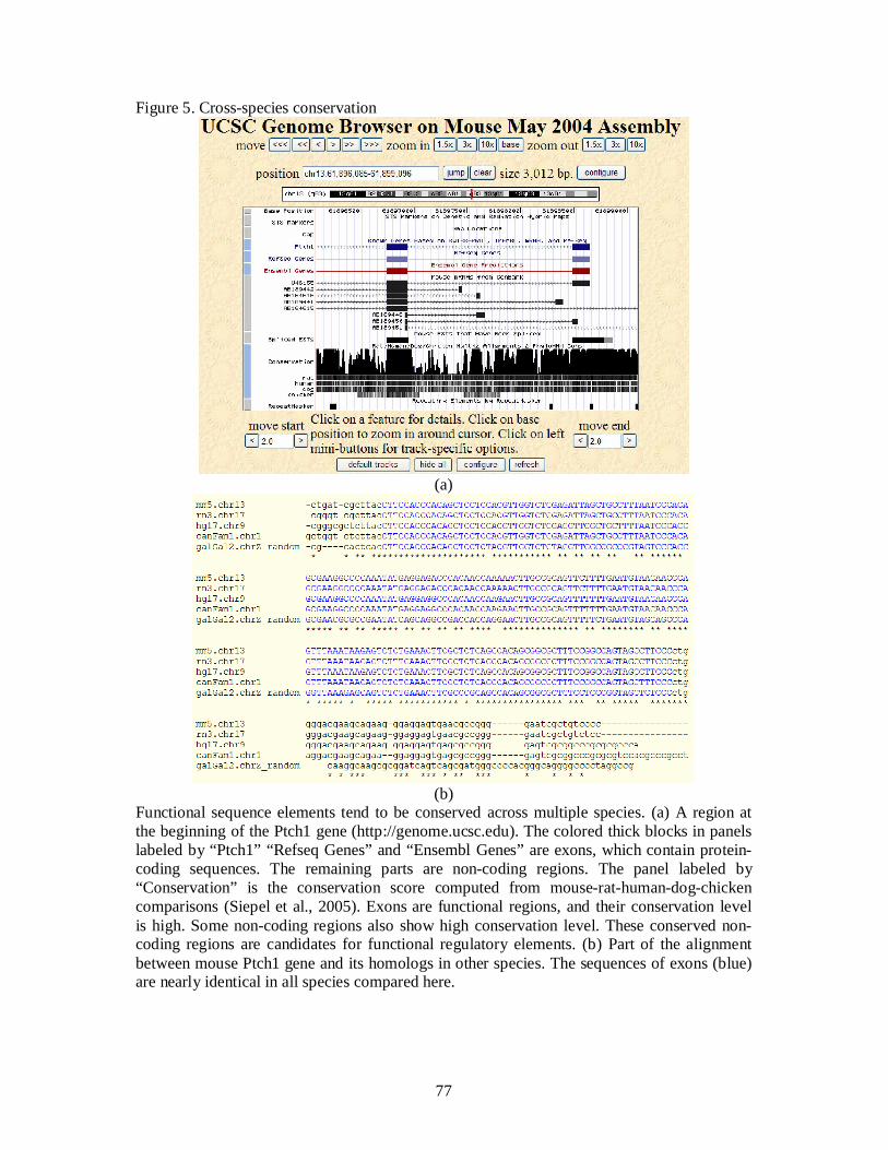
77

Figure 5. Cross-species conservation

(a)

(b)Functional sequence elements tend to be conserved across multiple species. (a) A region atthe beginning of the Ptch1 gene (http://genome.ucsc.edu). The colored thick blocks in panelslabeled by “Ptch1” “Refseq Genes” and “Ensembl Genes” are exons, which contain protein-coding sequences. The remaining parts are non-coding regions. The panel labeled by“Conservation” is the conservation score computed from mouse-rat-human-dog-chickencomparisons (Siepel et al., 2005). Exons are functional regions, and their conservation levelis high. Some non-coding regions also show high conservation level. These conserved non-coding regions are candidates for functional regulatory elements. (b) Part of the alignmentbetween mouse Ptch1 gene and its homologs in other species. The sequences of exons (blue)are nearly identical in all species compared here.

78

Figure 6. ChIP-chip experiment

(a)

(b)

(a) The ChIP-chip tiling array experiment tries to locate where transcription factors bind tothe genome. Immuno-precipitated (IP) DNA fragments are hybridized to probes evenlyspaced across the chromosome. Since IP fragments are amplified from DNA bound bytranscription factors, the hybridization signal will tell which part of the genome contains sitesfor transcription factors to bind. (b) A typical data structure of a ChIP-chip tiling arrayexperiment. Each point represents a signal for a probe. Probes are arranged by their physicallocations in the genome. The top panel shows raw hybridization signals for the IP samples(red) and the control samples (blue, green). The bottom panel shows the binding signalcomputed by GTRANS software.

79

Figure 7. Integrating various sources of information

For identifying cis-regulatory modules in higher organisms, one needs to integrate differenttypes of information. Expression profiles from microarray data can be used to cluster co-regulated genes. Cross-species comparisons and ChIP-chip experiments can help to narrowdown the search region. Module discovery algorithms that take clustering information ofTFBSs into account can then be applied to search for transcription factor binding sites andmotifs. After locating CRMs, the more challenging problem is to relate the locations andcombinatorial patterns of TFBSs back to gene functions. This area is largely unexplored.