Computational Biology

Jianfeng Feng

Warwick University

(many slides are from Dr. M. Lindquist)

http://www.dcs.warwick.ac.uk/~feng/Comp_Biol.html

Brain Science with Big Data:

Data Acquisition, machine learning and networks

Visualize your brain

http://venturebeat.com/2014/11/02/jonathan-rothbergs-butterfly-network-has-raised-100m-for-medical-imaging-tech/

Last week

• Image formation and k-space

•

Last week

• Image formation

• We can have two types of image : T1

TR

TE

t

By choosing short TR and TE, T1 weighted image is obtained

T1-weightedshort TR & TE

T2-weighted

long TR & TE

Last week

By choosing short TR and TE, T1 weighted image is obtained

T1-weightedshort TR & TE

T2-weighted

long TR & TE

Useful to access how many neurons are in your brain

Last week

By choosing long TR and TE, T2 or T2* weighted image is obtained

T1-weightedshort TR & TE

T2-weighted

long TR & TE

Useful to access the activity in your brain

Last week

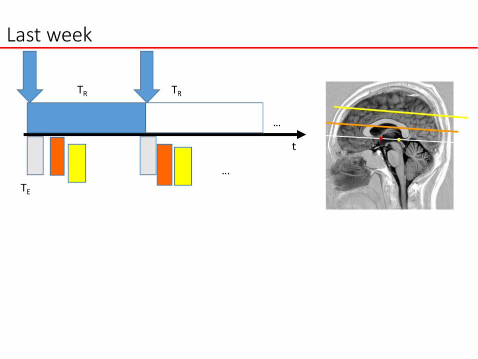
TRTR

TE

t

…

…

Last week

Last week

T1 vs T2 (T2*)

This week

Roughly understanding the preprocessing

You are able to use SPM to extract signals

5: fMRI Signal & Noise

MRI

• MRI studies brain anatomy.

– Structural (T1) images

– High spatial resolution

– Can distinguish different types of tissue

fMRI

• fMRI studies brain function.

– Functional (T2*) images

– Lower spatial resolution/ Higher temporal resolution

– Relate changes in signal to experimental manipulation

Functional MRI

• An fMRI experiment consists of a sequence of

individual MR images, where one can study

oxygenation changes in the brain across time.

BOLD fMRI

• The most common approach towards fMRI uses

the Blood Oxygenation Level Dependent (BOLD)

contrast.

• It allows us to measure the ratio of oxygenated to

deoxygenated hemoglobin in the blood.

• It doesn’t measure neuronal activity directly,

instead it measures the metabolic demands

(oxygen consumption) of active neurons.

BOLD Contrast

• Hemoglobin exists in two different states each

with different magnetic properties producing

different local magnetic fields. (Pauling 1936)

– Oxyhemoglobin is diamagnetic.

– Deoxyhemoglobin is paramagnetic.

• BOLD fMRI takes advantage of the difference in

T2* between oxygenated and deoxygenated

hemoglobin

(Seiji Ogawa, another Nobel prize?).

CellO2

Glucose

Cell

Capillary huge flowNeural activation

excitation reception

MR

sig

nal

(S)

TE t

RestActivation

T2*

Oxygenated Hb

BOLD Signal

BOLD Signal

• The change in the MR signal triggered by

instantaneous neuronal activity is known as the

hemodynamic response function.

• As neural activity increases, so does metabolic

demand for oxygen and nutrients.

• As oxygen is extracted from the blood, the

hemoglobin becomes paramagnetic which

creates distortions in the magnet field that cause

a T2* decrease (i.e. a faster decay of the signal).

• An over-compensation in blood flow

dilutes the concentration of

deoxyhemoglobin and tips the

balance towards oxyhemoglobin.– This leads to a peak in BOLD

signal about 4-6 s following

activation.

• After reaching its peak, the BOLD

signal decreases to an amplitude

below baseline level.– This poststimulus undershoot is due to a

combination of reduced blood flow and

increased blood volume.

BOLD Signal

HRF: hemodynamic

response function.

The strongest signal appears

5-6 seconds after activation.

HRF Properties

• Magnitude of signal changes is quite small

– 0.1 to 5%

– Hard to see in individual images

• Response is delayed and quite slow

– Extracting temporal information is tricky, but possible

– Even short events have a rather long response

• Exact shape of the response has been shown to

vary across subjects and regions.

Interpretation

• How well does BOLD signal reflect increases in

neural firing?

• The BOLD signal corresponds relatively closely

to the local electrical field potential surrounding a

group of cells.

• Demonstrations have shown that high-field BOLD

activity closely tracks the position of neural firing

and local field potentials.

• In plain words, the higher the fMRI signals, the

higher the neuronal firings.

LT I System

• The relationship between stimuli and the BOLD response

is often modeled using a linear time invariant (LTI) system.

– Here the neuronal activity acts as the input or impulse and the HRF acts as the impulse response function.

• In this framework the signal at time t, x(t), is modeled as theconvolution of a stimulus function v(t) and thehemodynamic response h(t), that is,

• In particular, if

t

dssthsvthvtx0

)()())(*()(

Convolution Example

Hemodynamic

Response

Function

Predicted Response

Experimental Stimulus Function

• The measured fMRI signal is corrupted by

random noise and various nuisance components

that arise due to hardware reasons and the

subjects themselves.

• Sources of noise:– Thermal motion of free electrons in the system.– Patient movement during the experiment.– Physiological effects, such as the subject’s heartbeat

and respiration.

– Low frequency signal drift.

fMRI Noise

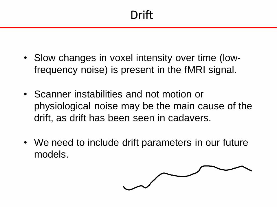
• Slow changes in voxel intensity over time (low-

frequency noise) is present in the fMRI signal.

• Scanner instabilities and not motion or

physiological noise may be the main cause of the

drift, as drift has been seen in cadavers.

• We need to include drift parameters in our future

models.

Drift

Issues

• Drift can have serious consequences:– Experimental conditions that vary slowly may be confused

with drift.

– Experimental designs should use high frequencies (more rapid alternations of stimulus on/off states).

• Bad Design: 2 min. rest 2 min. active

Typical Drift Pattern & Magnitude

Typical Signal Magnitude

... you’ll never detect this signal, due to the drift

A cautious note

• Neuroscientist Craig Bennett purchased a whole Atlantic salmon, took it to a lab at Dartmouth, and put it into an fMRI machine used to study the brain. The beautiful fish was to be the lab’s test object as they worked out some new methods.

• So, as the fish sat in the scanner, they showed it “a series of photographs depicting human individuals in social situations.” To maintain the rigor of the protocol (and perhaps because it was hilarious), the salmon, just like a human test subject, “was asked to determine what emotion the individual in the photo must have been experiencing.”

• The salmon, as Bennett’s poster on the test dryly notes, “was not alive at the time of scanning.”

• The result is completely nuts — but that’s actually exactly the point. Bennett, who is now a post-doc at the University of California, Santa Barbara, and his adviser, George Wolford, wrote up the work as a warning about the dangers of false positives in fMRI data. They wanted to call attention to ways the field could improve its statistical methods.

• IgNobel Prize in Neuroscience: The dead salmon study 2012

A cautious note

6: fMRI Data Structure

fMRI data

Spatial and temporal resolution

Terminology

Terminology

• MRI images are typically acquired in axial

slices- one at a time.

•This can be performed in either a sequential or interleaved manner.

•Together the slices make up a 3 dimensional brain volume.

Terminology

Terminology

•An experiment studies many subjects.

•Each subjects many be scanned during multiple

sessions.

•Each session consists a several runs.

•Each run consists of a series of brain volumes.

•Each volume is made up of multiple slices.

•Each slice contains many voxels.

•Each voxel has an intensity associate with it.

Terminology

Structures

fMRI data

• Each voxel has a corresponding time course.

Block Design

7: Pre-processing

Our module

Preprocessing Data Analysis

Raw Data

Acquisition

Slice-time Correction

Motion Correction,

Co-registration &

Normalization

Spatial Smoothing

LocalizingBrain Activity

Applications:

Clinical

Imaging genetics

……..

Reconstruction

DTI

Data Processing Pipeline

Connectivity

Experimental

Design

Linear Model

Grangercausality

Pre-Processing

•Prior to analysis, fMRI data undergoes a series of Preprocessing steps aimed at identifying and removing artifacts and validating model assumptions.

•The goals of preprocessing are – To minimize the influence of data acquisition and

physiological artifacts;

– To check statistical assumptions and transform the data to

meet assumptions;

– To standardize the locations of brain regions across

subjects to achieve validity and sensitivity in group analysis.

Pre-Processing

Preprocessing is performed both on the fMRI data and structural scans collected.

Pre-Processing Pipeline

•1. Visualization and Artifact Removal

•2. Slice Time Correction

•3. Motion Correction

•4. Physiological Corrections

•5. Co-registration

•6. Normalization

•7. Spatial Filtering

•8. Temporal Filtering

Pre-Processing Steps

•The first part of the preprocessing pipeline is to use exploratory techniques to investigate the raw image data and detect possible problems and artifacts.

• fMRI data often contain transient spike artifacts and slow drift over time.

•An exploratory technique (eye checking) can be used to look for spike-related artifacts.

Visualization and artifacts removing

•We often sample multiple slices of the brain during each individual repetition time (TR) to construct a brain volume.

•Typically each slice is sampled at a slightly different time points (i.e., 2D imaging; not 3D).

•Slice time correction shifts each voxel's time series so that they all appear to have been sampled simultaneously.

Slice time correction

Slice time correction

Slice time correction

Temporal Interpolation

•Use information from nearby time points to

estimate the amplitude of the MR signal at the

onset of the TR.

•Use a linear function for example.

Slice time correction

•Very small movements of the head during an experiment can be a major source of error if not treated correctly.

•When analyzing the time series associated with a voxel, we assume that it depicts the same region of the brain at every time point – Head motion may make this assumption incorrect.

•Can be corrected using a rigid body transformation.

Head motion

•The goal is to find the best possible alignment between an input image and some target image.

•To align the two images, one of them needs to be transformed.

•A rigid body transformation is used.

• It could involve 6 variable parameters, 3 sets of translations and 3 sets of rotations (6 DOF).

Motion correction

Linear transformations

•Rigid body (6 DOF) – translation and rotation

•Similarity (7 DOF) – translation, rotation and a single global scaling

•Affine(12 DOF) – translation, rotation, scaling and shearing.

Warping

Transformations where the equations relating the

coordinates of the images are non-linear.

Transformations

• The target image is usually defined to be the first (or mean) image in the fMRI time series.

•The goal is to find the set of parameters which minimizes some cost function that assesses similarity between the image and the target.

•Examples of cost functions include the sum of squared differences or mutual information.

Motion correction

Illustrations

•Next, a structural MRI collected in the beginning of the session is registered to the fMRI images in a process referred to as coregistration.

– Allows one to visualize single-subject task activations

overlaid on the individual’s anatomical information.

– Simplifies later transformation of the fMRI images to a

standard coordinate system.

Coregistration

•There are certain key differences between co-registration and motion correction. – Functional and structural images do not have the same

signal intensity in the same areas.

– Their shapes may differ.

• Use at least an affine transformation to perform

co-registration and the mutual information cost

function.

Coregistration

Coregistration

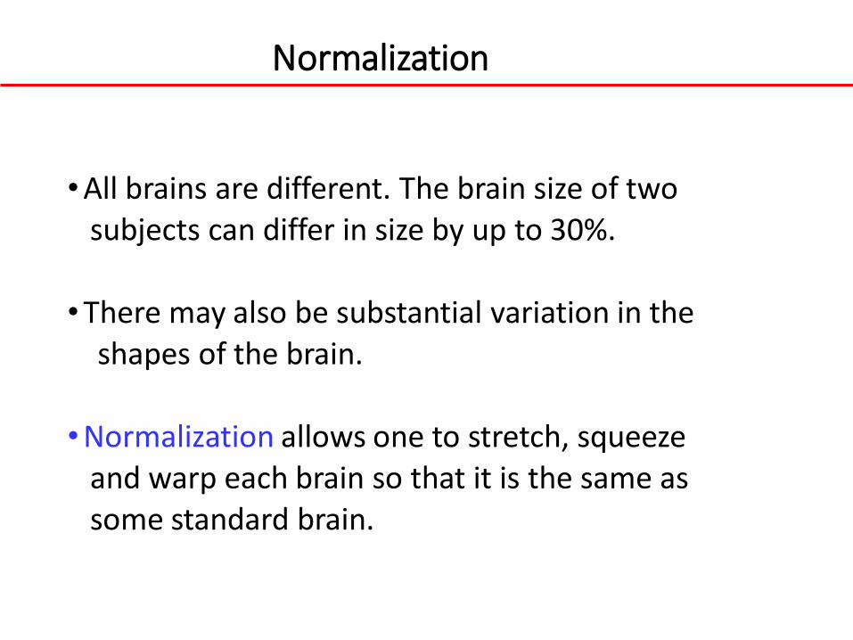
•All brains are different. The brain size of two subjects can differ in size by up to 30%.

•There may also be substantial variation in the shapes of the brain.

•Normalization allows one to stretch, squeeze and warp each brain so that it is the same as some standard brain.

Normalization

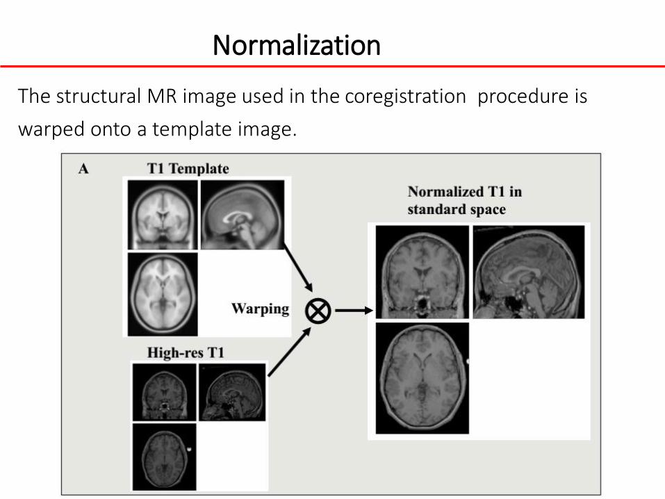
The structural MR image used in the coregistration procedure is

warped onto a template image.

Normalization

Pros

•Spatial locations can be reported and interpreted in a consistent manner.

•Results can be generalized to larger population

•Results can be compared across studies.

•Results can be averaged across subjects

Cons

•Reduces spatial resolution.

• Introduces potential errors.

Normalization

• Talairach space (Talairach and Tournoux,1988)

– Based on single subject (A cadaver of a 60 year old female)

– Based on a single hemisphere.

– The origin (0,0,0) is set at the Anterior Commisure.

– Oriented so that a line joining the Anterior

Commissure (AC) and the Posterior Commisure (PC) is

horizontal.

Brain atlases

• Montreal Neurological Institute (MNI)

– Combination of many MRI scans on normal

controls (152 in current standard).

– All right-handed subjects.

– More representative of population.

Brain Atlases

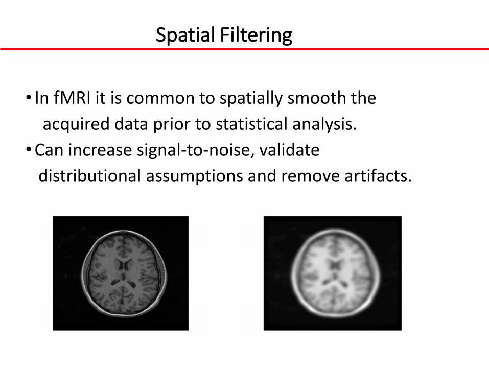
• In fMRI it is common to spatially smooth the

acquired data prior to statistical analysis.

•Can increase signal-to-noise, validate

distributional assumptions and remove artifacts.

Spatial Filtering

Pros

•May overcome limitations in the normalization by blurring any residual anatomical differences.

•Could increase the signal-to-noise ratio (SNR).

•May increase the validity of the statistical analysis.

•Required for Gaussian random fields.“

Cons

•The image resolution is reduced.

Spatial Filtering

The size of the kernel is determined by the

full width at half maximum (FWHM), which measures the width of the kernel at 50% of its peak value.

Spatial Filtering

•Typically, the amount of smoothing is chosen a priori and independently of the data.

•Furthermore, the same amount of smoothing is applied throughout the whole image.

•Adaptive smoothing could be an option.

– Non-stationary spatial Gaussian Markov random field.

– Smoothing varies across space and time.

Comments

Seminar II

• Learn to use SPM to preprocess data

• Have fun