Embed Size (px)
Citation preview
Guerino Mazzola • Gérard Milmeister •Jody Weissmann
Comprehensive Mathematicsfor Computer Scientists 1Sets and Numbers, Graphs and Algebra,Logic and Machines, Linear Geometry
With 118 Figures
(Second Edition)
This work is subject to copyright. All rights are reserved, whether the whole or part of thematerial is concerned, specifically the rights of translation, reprinting, reuse of illustrations,recitation, broadcasting, reproduction on microfilm or in any other way, and storage in databanks. Duplication of this publication or parts thereof is permitted only under theprovisions of the German Copyright Law of September 9, 1965, in its current version, andpermission for use must always be obtained from Springer-Verlag. Violations are liable forprosecution under the German Copyright Law.
Springer-Verlag is a part of Springer Science+Business Media
The use of general descriptive names, trademarks, etc. in this publication does not imply,even in the absence of a specific statement, that such names are exempt from the relevantprotective laws and regulations and therefore free for general use.
Cover Design: Erich Kirchner, HeidelbergTypesetting: Camera ready by the authors
Guerino MazzolaGérard MilmeisterJody Weissmann
Department of InformaticsUniversity ZurichWinterthurerstr. 1908057 Zurich, Switzerland
The text has been created using LATEX 2ε . The graphics were drawn using Dia, anopen-source diagramming software. The main text has been set in the Y&Y LucidaBright type family, the headings in Bitstream Zapf Humanist 601.
Library of Congress Control Number: 2006929906
ISBN 3-540-36873-6 Springer-Verlag Berlin Heidelberg New York
springer.com
Printed on acid-free paper SPIN: 11803911 40/3142/SPi - 543210
ISBN (First Edition) 3-540-20835-6
Mathematics Subject Classification (2000): 00A06
© Springer-Verlag Berlin Heidelberg 2006
Preface to the Second Edition
A second edition of a book is a success and an obligation at the same
time. We are satisfied that a number of university courses have been orga-
nized on the basis of the first volume of Comprehensive Mathematics for
Computer Scientists. The instructors recognized that the self-contained
presentation of a broad specturm of mathematical core topics is a firm
point of departure for a sustainable formal education in computer sci-
ence.
We feel obliged to meet the valuable feedback of the responsible in-
structors of such courses, in particular of Joel Young (Computer Science
Department, Brown University) who has provided us with numerous re-
marks on misprints, errors, or obscurities. We would like to express our
gratitude for these collaborative contributions. We have reread the entire
text and not only eliminated identified errors, but also given some addi-
tional examples and explications to statements and proofs which were
exposed in a too shorthand style.
A second edition of the second volume will be published as soon as the
errata, the suggestions for improvements, and the publisher’s strategy
are in harmony.
Zurich, Guerino Mazzola
June 2006 Gérard Milmeister
Jody Weissmann

Preface
The need for better formal competence as it is generated by a sound
mathematical education has been confirmed by recent investigations by
professional associations, but also by IT opinion leaders such as Niklaus
Wirth or Peter Wegner. It is rightly argued that programming skills are a
necessary but by far not sufficient qualification for designing and control-
ling the conceptual architecture of valid software. Often, the deficiency in
formal competence is compensated by trial and error programming. This
strategy may lead to uncontrolled code which neither formally nor ef-
fectively meets the given objectives. According to the global view such
bad engineering practice leads to massive quality breakdowns with cor-
responding economical consequences.
Improved formal competence is also urged by the object-oriented para-
digm which progressively requires a programming style and a design
strategy of high abstraction level in conceptual engineering. In this con-
text, the arsenal of formal tools must apply to completely different prob-
lem situations. Moreover, the dynamics and life cycle of hard- and soft-
ware projects enforce high flexibility of theorists and executives on all
levels of the computer science academia and IT industry. This flexibil-
ity can only be guaranteed by a propaedeutical training in a number of
typical styles of mathematical argumentation.
With this in mind, writing an introductory book on mathematics for com-
puter scientists is a somewhat delicate task. On the one hand, computer
science delves into the most basic machinery of human thought, such
as it is traced in the theory of Turing machines, rewriting systems and
grammars, languages, and formal logic. On the other hand, numerous ap-
plications of core mathematics, such as the theory of Galois fields (e.g.,
for coding theory), linear geometry (e.g., for computer graphics), or dif-
ferential equations (e.g., for simulation of dynamic systems) arise in any
VIII Preface
relevant topic of computational science. In view of this wide field of math-
ematical subjects the common practice is to focus one’s attention on
a particular bundle of issues and to presuppose acquaintance with the
background theory, or else to give a short summary thereof without any
further details.
In this book, we have chosen a different presentation. The idea was to set
forth and prove the entire core theory, from axiomatic set theory to num-
bers, graphs, algebraic and logical structures, linear geometry—in the
present first volume, and then, in the second volume, topology and cal-
culus, differential equations, and more specialized and current subjects
such as neural networks, fractals, numerics, Fourier theory, wavelets,
probability and statistics, manifolds, and categories.
There is a price to pay for this comprehensive journey through the over-
whelmingly extended landscape of mathematics: We decided to omit
any not absolutely necessary ramification in mathematical theorization.
Rather it was essential to keep the global development in mind and to
avoid an unnecessarily broad approach. We have therefore limited ex-
plicit proofs to a length which is reasonable for the non-mathematician.
In the case of lengthy and more involved proofs, we refer to further read-
ings. For a more profound reading we included a list of references to
original publications. After all, the student should realize as early as pos-
sible in his or her career that science is vitally built upon a network of
links to further knowledge resources.
We have, however, chosen a a modern presentation: We introduce the
language of commutative diagrams, universal properties and intuitionis-
tic logic as advanced by contemporary theoretical computer science in
its topos-theoretic aspect. This presentation serves the economy and el-
egance of abstraction so urgently requested by opinion leaders in com-
puter science. It also shows some original restatements of well-known
facts, for example in the theory of graphs or automata. In addition, our
presentation offers a glimpse of the unity of science: Machines, formal
concept architectures, and mathematical structures are intimately related
with each other.
Beyond a traditional “standalone” textbook, this text is part of a larger
formal training project hosted by the Department of Informatics at the
University of Zurich. The online counterpart of the text can be found
on http://math.ifi.unizh.ch. It offers access to this material and in-
cludes interactive tools for examples and exercises implemented by Java
Preface IX
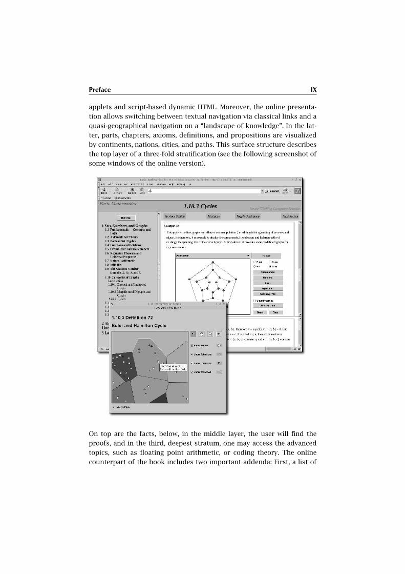
applets and script-based dynamic HTML. Moreover, the online presenta-
tion allows switching between textual navigation via classical links and a
quasi-geographical navigation on a “landscape of knowledge”. In the lat-
ter, parts, chapters, axioms, definitions, and propositions are visualized
by continents, nations, cities, and paths. This surface structure describes
the top layer of a three-fold stratification (see the following screenshot of
some windows of the online version).
On top are the facts, below, in the middle layer, the user will find the
proofs, and in the third, deepest stratum, one may access the advanced
topics, such as floating point arithmetic, or coding theory. The online
counterpart of the book includes two important addenda: First, a list of

X Preface
errata can be checked out. The reader is invited to submit any error en-
countered while reading the book or the online presentation. Second, the
subject spectrum, be it in theory, examples, or exercises, is constantly up-
dated and completed and, if appropriate, extended. It is therefore recom-
mended and beneficial to work with both, the book and its online coun-
terpart.
This book is a result of an educational project of the E-Learning Center
of the University of Zurich. Its production was supported by the Depart-
ment of Informatics, whose infrastructure we were allowed to use. We
would like to express our gratitude to these supporters and hope that
the result will yield a mutual profit: for the students in getting a high
quality training, and for the authors for being given the chance to study
and develop a core topic of formal education in computer science. We
also deeply appreciate the cooperation with the Springer Publishers, es-
pecially with Clemens Heine, who managed the book’s production in a
completely efficient and unbureaucratic way.
Zurich, Guerino Mazzola
February 2004 Gérard Milmeister
Jody Weissmann

Contents
I Sets, Numbers, and Graphs 1
1 Fundamentals—Concepts and Logic 3
1.1 Propositional Logic . . . . . . . . . . . . . . . . . . . . . . . . . . . . . . . . . . . . . . 4
1.2 Architecture of Concepts . . . . . . . . . . . . . . . . . . . . . . . . . . . . . . . . 8
2 Axiomatic Set Theory 15
2.1 The Axioms . . . . . . . . . . . . . . . . . . . . . . . . . . . . . . . . . . . . . . . . . . . . . 17
2.2 Basic Concepts and Results . . . . . . . . . . . . . . . . . . . . . . . . . . . . . . 20
3 Boolean Set Algebra 25
3.1 The Boolean Algebra of Subsets . . . . . . . . . . . . . . . . . . . . . . . . . . 25
4 Functions and Relations 29
4.1 Graphs and Functions . . . . . . . . . . . . . . . . . . . . . . . . . . . . . . . . . . . 29
4.2 Relations . . . . . . . . . . . . . . . . . . . . . . . . . . . . . . . . . . . . . . . . . . . . . . . . 41
5 Ordinal and Natural Numbers 45
5.1 Ordinal Numbers . . . . . . . . . . . . . . . . . . . . . . . . . . . . . . . . . . . . . . . . 45
5.2 Natural Numbers . . . . . . . . . . . . . . . . . . . . . . . . . . . . . . . . . . . . . . . . 50
6 Recursion Theorem and Universal Properties 55
6.1 Recursion Theorem . . . . . . . . . . . . . . . . . . . . . . . . . . . . . . . . . . . . . . 56
6.2 Universal Properties . . . . . . . . . . . . . . . . . . . . . . . . . . . . . . . . . . . . . 58
6.3 Universal Properties in Relational Database Theory . . . . . . 66
7 Natural Arithmetic 73
7.1 Natural Operations . . . . . . . . . . . . . . . . . . . . . . . . . . . . . . . . . . . . . . 73
7.2 Euclid and the Normal Forms . . . . . . . . . . . . . . . . . . . . . . . . . . . . 76
8 Infinities 79
8.1 The Diagonalization Procedure . . . . . . . . . . . . . . . . . . . . . . . . . . 79
XII Contents
9 The Classical Number Domains Z, Q, R, and C 81
9.1 Integers Z . . . . . . . . . . . . . . . . . . . . . . . . . . . . . . . . . . . . . . . . . . . . . . . 82
9.2 Rationals Q . . . . . . . . . . . . . . . . . . . . . . . . . . . . . . . . . . . . . . . . . . . . . 87
9.3 Real Numbers R . . . . . . . . . . . . . . . . . . . . . . . . . . . . . . . . . . . . . . . . . 90
9.4 Complex Numbers C . . . . . . . . . . . . . . . . . . . . . . . . . . . . . . . . . . . . 102
10 Categories of Graphs 107
10.1 Directed and Undirected Graphs . . . . . . . . . . . . . . . . . . . . . . . . . 108
10.2 Morphisms of Digraphs and Graphs . . . . . . . . . . . . . . . . . . . . . 114
10.3 Cycles . . . . . . . . . . . . . . . . . . . . . . . . . . . . . . . . . . . . . . . . . . . . . . . . . . . 125
11 Construction of Graphs 129
12 Some Special Graphs 137
12.1n-ary Trees . . . . . . . . . . . . . . . . . . . . . . . . . . . . . . . . . . . . . . . . . . . . . . 137
12.2 Moore Graphs . . . . . . . . . . . . . . . . . . . . . . . . . . . . . . . . . . . . . . . . . . . 139
13 Planarity 143
13.1 Euler’s Formula for Polyhedra . . . . . . . . . . . . . . . . . . . . . . . . . . . 143
13.2 Kuratowski’s Planarity Theorem . . . . . . . . . . . . . . . . . . . . . . . . . 147
14 First Advanced Topic 149
14.1 Floating Point Arithmetic . . . . . . . . . . . . . . . . . . . . . . . . . . . . . . . . 149
14.2 Example for an Addition . . . . . . . . . . . . . . . . . . . . . . . . . . . . . . . . . 154
II Algebra, Formal Logic, and Linear Geometry 157
15 Monoids, Groups, Rings, and Fields 159
15.1 Monoids . . . . . . . . . . . . . . . . . . . . . . . . . . . . . . . . . . . . . . . . . . . . . . . . . 159
15.2 Groups . . . . . . . . . . . . . . . . . . . . . . . . . . . . . . . . . . . . . . . . . . . . . . . . . . 163
15.3 Rings . . . . . . . . . . . . . . . . . . . . . . . . . . . . . . . . . . . . . . . . . . . . . . . . . . . . 171
15.4 Fields . . . . . . . . . . . . . . . . . . . . . . . . . . . . . . . . . . . . . . . . . . . . . . . . . . . 177
16 Primes 181
16.1 Prime Factorization . . . . . . . . . . . . . . . . . . . . . . . . . . . . . . . . . . . . . . 181
16.2 Roots of Polynomials and Interpolation . . . . . . . . . . . . . . . . . . 186
17 Formal Propositional Logic 191
17.1 Syntactics: The Language of Formal Propositional Logic . . 193
17.2 Semantics: Logical Algebras. . . . . . . . . . . . . . . . . . . . . . . . . . . . . . 196
17.3 Signification: Valuations . . . . . . . . . . . . . . . . . . . . . . . . . . . . . . . . . 200
17.4 Axiomatics . . . . . . . . . . . . . . . . . . . . . . . . . . . . . . . . . . . . . . . . . . . . . . 203
Contents XIII
18 Formal Predicate Logic 209
18.1 Syntactics: First-order Language . . . . . . . . . . . . . . . . . . . . . . . . . 211
18.2 Semantics: Σ-Structures . . . . . . . . . . . . . . . . . . . . . . . . . . . . . . . . . . 217
18.3 Signification: Models . . . . . . . . . . . . . . . . . . . . . . . . . . . . . . . . . . . . . 218
19 Languages, Grammars, and Automata 223
19.1 Languages . . . . . . . . . . . . . . . . . . . . . . . . . . . . . . . . . . . . . . . . . . . . . . . 224
19.2 Grammars . . . . . . . . . . . . . . . . . . . . . . . . . . . . . . . . . . . . . . . . . . . . . . . 229
19.3 Automata and Acceptors . . . . . . . . . . . . . . . . . . . . . . . . . . . . . . . . 243
20 Categories of Matrixes 261
20.1 What Matrixes Are . . . . . . . . . . . . . . . . . . . . . . . . . . . . . . . . . . . . . . . 262
20.2 Standard Operations on Matrixes . . . . . . . . . . . . . . . . . . . . . . . . 265
20.3 Square Matrixes and their Determinant . . . . . . . . . . . . . . . . . . 271
21 Modules and Vector Spaces 279
22 Linear Dependence, Bases, and Dimension 287
22.1 Bases in Vector Spaces . . . . . . . . . . . . . . . . . . . . . . . . . . . . . . . . . . . 288
22.2 Equations . . . . . . . . . . . . . . . . . . . . . . . . . . . . . . . . . . . . . . . . . . . . . . . 295
22.3 Affine Homomorphisms . . . . . . . . . . . . . . . . . . . . . . . . . . . . . . . . . 296
23 Algorithms in Linear Algebra 303
23.1 Gauss Elimination . . . . . . . . . . . . . . . . . . . . . . . . . . . . . . . . . . . . . . . 303
23.2 The LUP Decomposition . . . . . . . . . . . . . . . . . . . . . . . . . . . . . . . . . 307
24 Linear Geometry 311
24.1 Euclidean Vector Spaces . . . . . . . . . . . . . . . . . . . . . . . . . . . . . . . . . 311
24.2 Trigonometric Functions from Two-Dimensional Rotations 320
24.3 Gram’s Determinant and the Schwarz Inequality . . . . . . . . . 323
25 Eigenvalues, the Vector Product, and Quaternions 327
25.1 Eigenvalues and Rotations . . . . . . . . . . . . . . . . . . . . . . . . . . . . . . . 327
25.2 The Vector Product . . . . . . . . . . . . . . . . . . . . . . . . . . . . . . . . . . . . . . 331
25.3 Quaternions . . . . . . . . . . . . . . . . . . . . . . . . . . . . . . . . . . . . . . . . . . . . . 333
26 Second Advanced Topic 343
26.1 Galois Fields . . . . . . . . . . . . . . . . . . . . . . . . . . . . . . . . . . . . . . . . . . . . 343
26.2 The Reed-Solomon (RS) Error Correction Code . . . . . . . . . . . 349
26.3 The Rivest-Shamir-Adleman (RSA) Encryption Algorithm . 353
A Further Reading 357
XIV Contents
B Bibliography 359
Index 363
Volume II
III Topology and Calculus
Limits and Topology, Differentiability, Inverse and Implicit Func-
tions, Integration, Fubini and Changing Variables, Vector Fields,
Fixpoints, Main Theorem of ODEs
IV Selected Higher Subjects
Numerics, Probability and Statistics, Splines, Fourier, Wavelets,
Fractals, Neural Nets, Global Coordinates and Manifolds, Cate-
gories, Lambda Calculus

PART I
Sets, Numbers, and Graphs
CHAPTER 1
Fundamentals—
Concepts and Logic
Die Welt ist alles, was der Fall ist.
Ludwig Wittgenstein
“The world is everything that is the case” — this is the first tractatus in
Ludwig Wittgenstein’s Tractatus Logico-Philosophicus.
In science, we want to know what is true, i.e., what is the case, and what is
not. Propositions are the theorems of our language, they are to describe
or denote what is the case. If they do, they are called true, otherwise they
are called false. This sounds a bit clumsy, but actually it is pretty much
what our common sense tells us about true and false statements. Some
examples may help to clarify things:
“This sentence contains five words”
This proposition describes something which is the case, therefore it
is a true statement.
“Every human being has three heads”
Since I myself have only one head (and I assume this is the case with
you as well), this proposition describes a situation which is not the
case, therefore it is false.
In order to handle propositions precisely, science makes use of two fun-
damental tools of thought:
4 Fundamentals—Concepts and Logic
• Propositional Logic
• Architecture of Concepts
These tools aid a scientist to construct accurate concepts and to formu-
late new true propositions from old ones.
The following sections may appear quite diffuse to the reader; some
things will seem to be obviously true, other things will perhaps not make
much sense to start with. The problem is that we have to use our natural
language for the task of defining things in a precise way. It is only by
using these tools that we can define in a clear way what a set is, what
numbers are, etc.
1.1 Propositional Logic
Propositional logic helps us to navigate in a world painted in black and
white, a world in which there is only truth or falsehood, but nothing in
between. It is a boiled down version of common sense reasoning. It is the
essence of Sherlock Holmes’ way of deducing that Professor Moriarty was
the mastermind behind a criminal organization (“Elementary, my dear
Watson”). Propositional logic builds on the following two propositions,
which are declared to be true as basic principles (and they seem to make
sense. . . ):
Principle of contradiction (principium contradictionis)
A proposition is never true and false at the same time.
Principle of the excluded third (tertium non datur)
A proposition is either true or false—there is no third possibility.
In other words, in propositional logic we work with statements that are
either true (T) or false (F), no more and no less. Such a logic is also known
as absolute logic.
In propositional logic there are also some operations which are used to
create new propositions from old ones:
Logical Negation
The negation of a true proposition is a false proposition, the negation
of a false proposition is a true proposition. This operation is also
called ‘NOT’.

1.1 Propositional Logic 5
Logical Conjunction
The conjunction of two propositions is true if and only if both pro-
positions are true. In all other cases it is false. This operation is also
called ‘AND’.
Logical Disjunction
The disjunction of two propositions is true if at least one of the
propositions is true. If both propositions are false, the disjunction
is false, too. This operation is also known as ‘OR’.
Logical Implication
A proposition P1 implies another proposition P2 if P2 is true when-
ever P1 is true. This operation is also known as ‘IMPLIES’.
Often one uses so-called truth tables to show the workings of these oper-
ations. In these tables, A stands for the possible truth values of a propo-
sition A, and B stands for the possible truth values of a proposition B.
The rows labeled “A AND B” and “A OR B” contain the truth value of the
conjunction and disjunction of the propositions.
A NOT A
F T
T F
A B A AND B
F F F
F T F
T F F
T T T
A B A OR B
F F F
F T T
T F T
T T T
A B A IMPLIES B
F F T
F T T
T F F
T T T
Let us look at a few examples.
1. Let proposition A be “The ball is red”. The negation of A, (i.e., NOT
A) is “It is not the case that the ball is red”. So, if the ball is actually
green, that means thatA is false and that NOTA is true.
2. Let proposition A be “All balls are round” and proposition B “All
balls are green”. Then the conjunctionA AND B of A and B is false,
because there are balls that are not green.
3. Using the same propositions, the disjunction of A and B, A OR B is
true.
4. For any proposition A, A AND (NOT A) is always false (principle of
contradiction).
5. For any proposition A, A OR (NOT A) is always true (principle of
excluded third).
6 Fundamentals—Concepts and Logic
In practice it is cumbersome to say: “The proposition It rains is true”.
Instead, one just says: “It rains.” Also, since the formal combination of
propositions by the above operators is often an overhead, we mostly use
the common language denotation, such as: “2 = 3 is false” instead of
“NOT (2 = 3)” or: “It’s raining or/and I am tired.” instead of “It’s rain-
ing OR/AND I am tired”, or: “If it’s raining, then I am tired” instead of
“It’s raining IMPLIES I am tired.” Moreover, we use the mathematical ab-
breviation “A iff B” for “(A IMPLIES B) AND (B IMPLIES A)”. Observe that
brackets (. . .) are used in order to make the grouping of symbols clear if
necessary.
The operations NOT, AND, OR, and IMPLIES have a number of properties
which are very useful for simplifying complex combinations of these op-
erations. Let P , Q, and R be truth values. Then the following properties
hold:
Commutativity of AND
P AND Q is the same as Q AND P .
Commutativity of OR
P OR Q is the same as Q OR P .
Associativity of AND
(P AND Q) AND R is the same as P AND (Q AND R).
One usually omits the parentheses and writes P AND Q AND
R.
Associativity of OR
(P OR Q) OR R is the same as P OR (Q OR R).
One usually omits the parentheses and writes P OR Q OR R.
De Morgan’s Law for AND
NOT (P AND Q) is the same as (NOT P ) OR (NOT Q).
De Morgan’s Law for OR
NOT (P OR Q) is the same as (NOT P ) AND (NOT Q).
Distributivity of AND over OR
P AND (Q OR R) is the same as (P AND Q) OR (P AND R).
Distributivity of OR over AND
P OR (Q AND R) is the same as (P OR Q) AND (P OR R).
Contraposition
P IMPLIES Q is the same as (NOT Q) IMPLIES (NOT P ).
1.1 Propositional Logic 7
Idempotency of AND
P is the same as P AND P .
Idempotency of OR
P is the same as P OR P .
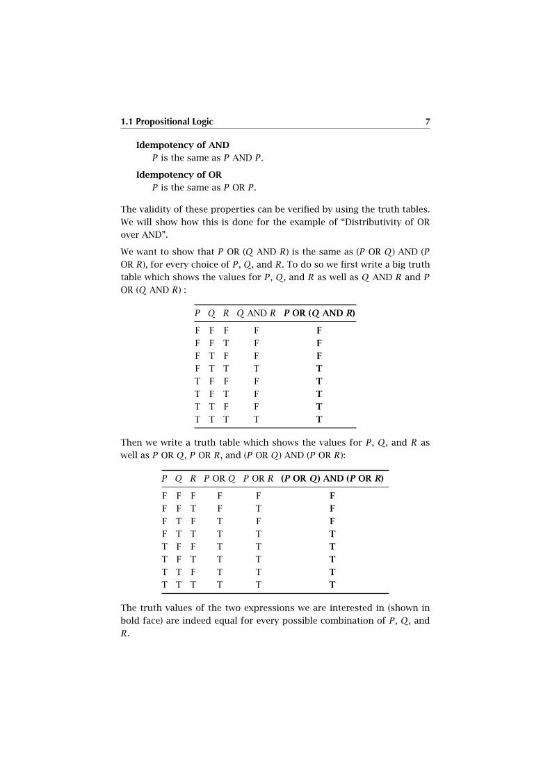
The validity of these properties can be verified by using the truth tables.
We will show how this is done for the example of “Distributivity of OR
over AND”.
We want to show that P OR (Q AND R) is the same as (P OR Q) AND (P
OR R), for every choice of P , Q, and R. To do so we first write a big truth
table which shows the values for P , Q, and R as well as Q AND R and P
OR (Q AND R) :
P Q R Q AND R P OR (Q AND R)
F F F F F
F F T F F
F T F F F
F T T T T
T F F F T
T F T F T
T T F F T
T T T T T
Then we write a truth table which shows the values for P , Q, and R as
well as P OR Q, P OR R, and (P OR Q) AND (P OR R):
P Q R P OR Q P OR R (P OR Q ) AND (P OR R)
F F F F F F
F F T F T F
F T F T F F
F T T T T T
T F F T T T
T F T T T T
T T F T T T
T T T T T T
The truth values of the two expressions we are interested in (shown in
bold face) are indeed equal for every possible combination of P , Q, and
R.

8 Fundamentals—Concepts and Logic
The verification of the remaining properties is left as an exercise for the
reader.
1.2 Architecture of Concepts
In order to formulate unambiguous propositions, we need a way to de-
scribe the concepts we want to make statements about. An architecture of
concepts deals with the question: “How does one build a concept?” Such
an architecture defines ways to build new concepts from already existing
concepts. Of course one has to deal with the question where to anchor
the architecture, in other words, what are the basic concepts and how
are they introduced. This can be achieved in two different ways. The first
uses the classical approach of undefined primary concepts, the second
avoids primary concepts by circular construction. This second approach
is the one that is used for building the architecture of set theory in this
book.
1. A concept has a name, for example, “Number” or “Set” are names of
certain concepts.
2. Concepts have components, which are concepts, too.
These components are used to construct a concept.
3. There are three fundamental principles of how to combine such com-
ponents:
• Conceptual Selection: requires one component
• Conceptual Conjunction: requires one or two components
• Conceptual Disjunction: requires two components
4. Concepts have instances (examples), which have the following prop-
erties:
• Instances have a name
• Instances have a value
The construction principles mentioned above are best described using
instances:
The value of an instance of a concept constructed as a selection is the
collection of the references to selected instances of the component.
1.2 Architecture of Concepts 9
The value of an instance of a concept constructed as a conjunction is the
sequence of the references to the instances of each component.
The value of an instance of a concept constructed as a disjunction is a
reference to an instance of one of the components.
Perhaps some examples will clarify those three construction principles.
A selection is really a selection in its common sense meaning: You point
at a thing and say, “I select this”, you point at another thing and say “I
select this, too” and so on.
One example for a conjunction are persons’ names which (at least in the
western world) always consists of a first name and a family name. An-
other example is given by the points in the plane: every point is defined
by an x- and a y-coordinate.
A disjunction is a simple kind of “addition”: An instance of the disjunc-
tion of all fruits and all animals is either a fruit or an animal.
Notation
If we want to write about concepts and instances, we need an expressive
and precise notation.
Concept: ConceptName.ConstructionPrinciple(Component(s))
This means that we first write the concept’s name followed by a dot.
After the dot we write the construction principle (Selection, Conjunc-
tion, or Disjunction) used to construct the concept. Finally we add
the component or components which were used for the construction
enclosed in brackets.
Instance: InstanceName@ConceptName(Value)
In order to write down an instance, we write the instance’s name fol-
lowed by an ‘@’. After this, the name of the concept is added, followed
by a value enclosed in brackets. In the case of a disjunction, a semi-
colon directly following the value denotes the first component, and a
semicolon preceding the value denotes the second component.
Very often it is not possible to write down the entire information needed
to define a concept. In most cases one cannot write down components
and values explicitly. Therefore, instead of writing the concept or in-
stance, one only writes its name. Of course, this presupposes that these
10 Fundamentals—Concepts and Logic
objects can be identified by a name, i.e., there are enough names to distin-
guish these objects from one another. Thus if two concepts have identi-
cal names, then they have identical construction principles and identical
components. The same holds for instances: identicals name mean identi-
cal concepts and identical values.
By identifying names with objects one can say “let X be a concept” or “let
z be an instance”, meaning that X and z are the names of such objects
that refer to those objects in a unique way.
Here are some simple examples for concepts and instances:
CitrusFruits.Disjunction(Lemons, Oranges)
The concept CitrusFruit consists of the concepts Lemons and Or-
anges.
MyLemon@Citrusfruits(Lemon2; )
MyLemon is an instance of the concept CitrusFruit, and has the value
Lemon2 (which is itself an instance of the concept Lemons).
YourOrange@Citrusfruits(; Orange7)
YourOrange is an instance of the concept CitrusFruits, and has the
value Orange7 (which is itself an instance of the concept Oranges).
CompleteNames.Conjunction(FirstNames, FamilyNames)
The concept CompleteNames is a conjunction of the concept First-
Names and FamilyNames.
MyName@CompleteNames(John; Doe)
MyName is an instance of the concept CompleteNames, and has the
value John; Doe.
SmallAnimals.Selection(Animals)
The concept SmallAnimals is a selection of the concept Animals.
SomeInsects@SmallAnimals(Ant, Ladybug, Grasshopper)
SomeInsects is an instance of the concept SmallAnimals and has the
value Ant, Ladybug, Grasshopper.
Mathematics
The environment in which this large variety of concepts and propositions
is handled is Mathematics.
1.2 Architecture of Concepts 11
With the aid of set theory Mathematics is made conceptually precise and
becomes the foundation for all formal tools. Especially formal logic is
only possible on this foundation.
In Mathematics the existence of a concept means that it is conceivable
without any contradiction. For instance, a set exists if it is conceivable
without contradiction. Most of the useful sets exist (i.e., are conceiv-
able without contradiction), but one may conceive sets which don’t ex-
ist. An example of such a set is the subject of the famous paradox ad-
vanced by Bertrand Russell: the set containing all sets that do not contain
themselves—does this set contain itself, or not?
Set theory must be constructed successively to form an edifice of con-
cepts which is conceivable without any contradictions.
In this section we will first show how one defines natural numbers using
concepts and instances. After that, we go on to create set theory from
“nothing”.
Naive Natural Numbers
The natural numbers can be conceptualized as follows:
Number.Disjunction(Number, Terminator)
Terminator.Conjunction(Terminator)
The concept Number is defined as a disjunction of itself with a concept
Terminator, the concept Terminator is defined as a conjunction of itself
(and nothing else). The basic idea is to define a specific natural number
as the successor of another natural number. This works out for 34, which
is the successor of 33, and also for 786657, which is the successor of
786656. But what about 0? The number zero is not the successor of any
other natural number. So in a way we use the Terminator concept as a
starting point, and successively define each number (apart from 0) as the
successor of the preceding number. The fact that the concept Termina-
tor is defined as a conjunction of itself simply means: “Terminator is a
thing”. This is a first example of a circular construction used as an artifice
to ground the definition of natural numbers.
Now let us look at some instances of these concepts:
12 Fundamentals—Concepts and Logic
t@Terminator(t)
In natural language: the value of the instance t of Terminator is itself.
This is a second application of circularity.
0@Number(; t)
The instance of Number which we call 0 has the value t;.
1@Number(0; )
The instance of Number which we call 1 has the value 0;.
2@Number(1; )
The instance of Number which we call 2 has the value 1;.
If we expand the values of the numbers which are neither 0 nor t, we get
• the value of 1 is 0;
• the value of 2 is 1; which is 0;;
• the value of 3 is 2; which is 0;;;
• etc.
This could be interpreted by letting the semicolon stand for the operation
“successor of”, thus 3 is the successor of the successor of the successor
of 0.
Pure Sets
The pure sets are defined in the following circular way:
Set.Selection(Set)
Here, we say that a set is a selection of sets. Since one is allowed to
select nothing in a conceptual selection, there is a starting point for this
circularity. Let us look at some instances again:
∅@Set()
Here we select nothing from the concept Set. We therefore end up
with the empty set.
1@Set(∅)
Since ∅ is a set we can select it from the concept Set. The value of 1
is a set consisting of one set.

1.2 Architecture of Concepts 13
2@Set(∅, 1)
Here we select the two sets we have previously defined. The value of
2 is a set consisting of two sets.
Elements of the Mathematical Prose
In Mathematics, there is a “catechism” of true statements, which are
named after their relevance in the development of the theory.
An axiom is a statement which is not proved to be true, but supposed
to be so. In a second understanding, a theory is called axiomatic if its
concepts are abstractions from examples which are put into generic defi-
nitions in order to develop a theory from a given type of concepts.
A definition is used for building—and mostly also for introducing a sym-
bolic notation for—a concept which is described using already defined
concepts and building rules.
A lemma is an auxiliary statement which is proved as a truth prelimi-
nary to some more important subsequent true statement. A corollary is
a true statement which follows without significant effort from an already
proved statement. Ideally, a corollary should be a straightforward conse-
quence of a more difficult statement. A sorite is a true statement, which
follows without significant effort from a given definition. A proposition is
an important true statement, but less important than a theorem, which is
the top spot in this nomenclature.
A mathematical proof is the logical deduction of a true statement B from
another true statement C. Logical deduction means that the theorems
of absolute logic are applied to establish the truth of B, knowing the
truth of C. The most frequent procedure is to use as the true statement
C the truth of A and the truth of A IMPLIES B, in short, the truth of
A AND (A IMPLIES B). Then B is true since the truth of the implica-
tion with the true antecedent A can only hold with B also being true.
This is the so-called modus ponens. This scheme is also applied for indi-
rect proofs, i.e., we use the true fact (NOT B) IMPLIES (NOT A), which is
equivalent toA IMPLIES B (contraposition, see also properties on page 6).
Now, by the principle of the excluded third and the principle of contra-
diction, either B or NOT B will be true, but not both at the same time.
Then the truth of NOT B enforces the truth of NOTA. But by the princi-
ple of contradiction, A and NOT A cannot be both true, and since A is
true, NOT B cannot hold, and therefore, by the principles of the excluded
14 Fundamentals—Concepts and Logic
third and of contradiction, B is true. There are also more technical proof
techniques, such as the proof by induction, but logically speaking, they
are all special cases of the general scheme just described.
In this book, the end of a proof is marked by the symbol �.
CHAPTER 2
Axiomatic Set Theory
Axiomatic set theory is the theory of pure sets, i.e., it is built on a set
concept which refers to nothing else but itself. One then states a number
of axioms, i.e., propositions which are supposed to be true for sets (i.e.,
instances of the set concept). On this axiomatic basis, the whole mathe-
matical concept framework is built, leading from elementary numbers to
the most complex structures, such as differential equations or manifolds.
The concept of “pure sets” was already given in our introduction 1.2:
Set.Selection(Set)
and the instance scheme
SetName@Set(Value)
where the value is described such that each reference is uniquely identi-
fied.
Notation 1 If a set X has a set x amongst its values, one writes “x ∈ X”
and one says “x is an element of X”. If it is not the case that “x ∈ X”, one
writes “x ∉ X”.
If it is possible to write down the elements of a set explicitly, one uses curly
brackets: Instead of “A@Set(a, b, c, . . . z)” one writes1 “A = {a,b, c, . . . z}”.For example, the empty set is ∅ = {}.If there is an attribute F which characterizes the elements of a set A one
writes “A = {x | F(x)}”, where “F(x)” stands for “x has attribute F”.
1 In the context of set theory, this traditional notation is preferred, but can
always be reduced to the more generic @-notation.
16 Axiomatic Set Theory
Definition 1 (Subsets and equality of sets) Let A and B be sets. We say
that A is a subset of B, and we write “A ⊂ B” if for every set x the propo-
sition (x ∈ A IMPLIES x ∈ B) is true.
One says that A equals B and writes “A = B” if the proposition (A ⊂B AND B ⊂ A) is true. If “A ⊂ B” is false, one writes “A 6⊂ B”. If “A = B” is
false, one writes “A ≠ B”. If A ⊂ B, but A ≠ B, one also writes “A ⊊ B”.
A subset A ⊂ B is said to be the smallest subset of B with respect to a
property P , if it has this property and is a subset of every subset X ⊂ Bhaving this property P .
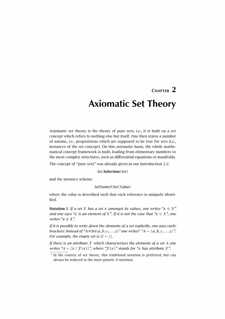
Fig. 2.1. In order to give the reader a better intuition about sets, we
visualize them as bags, while their elements are shown as smaller bags—
or as symbols for such elements—contained in larger ones. For example,
∅ is drawn as the empty bag. The set in this figure is {∅, {∅}}.
Example 1 Let A = {a,b, {c, d}}. Then a ∈ A and {c, d} ∈ A, but c ∉ A;
{a,b} ⊂ A and {{c, d}} ⊂ A, but {c, d} 6⊂ A.
In these examples, sets are specified by enumerating their elements. For
an example of the use of an attribute for characterizing the members of a
set consider the propositional attributeA(x) defined by “x is a member
of the Apollo 11 crew”. Then {x | A(x)} = {Armstrong,Aldrin,Collins}.The number of objects specified by an attribute need not be limited. Thus
the set {x | N (x)}, where N (x) is defined by “x is a number”, cannot
be written down by means of enumeration alone.
For any set X we have {} ⊂ X. To prove this, one has to show that the
proposition (x ∈ {} IMPLIES x ∈ X) is true. Since the empty set does
not have any elements, the left hand side of the implication is false. A

2.1 The Axioms 17
quick glance at the truth tables on page 5 shows that in this case the
implication as a whole is true, irrespective of the truth value of the right
hand side. This reasoning is to be kept in mind when dealing with the
empty set.
Example 2 Two empty sets A = {} and B = {} are equal. This is the case
because the previous example tells us that A ⊂ B and B ⊂ A, and this is
simply the definition for A = B.
It is impossible to decide whether two circular sets I = {I} and J = {J}are equal.
2.1 The Axioms
Axiomatic set theory is defined by two components: Its objects are pure
sets, and the instances of such sets are required to satisfy a number of
properties, the axioms, which cannot be deduced by logical reasoning,
but must be claimed. It is hard to show that such axioms lead to math-
ematically existing sets. We circumvent this problem by stating a list of
common axioms.
The following collection of axioms is a variant of the collection proposed
by Ernst Zermelo and Abraham Fraenkel (ZFC, for short). However, we do
not include the axiom of foundation since modern theoretical computer
science has a need for circular sets which this axiom excludes. Finally,
we replace the axiom of extentionality by the axiom of equality, which
respects more properly the difference between equality and identity. For
a discussion of the classical ZFC axioms, see [20].
Axiom 1 (Axiom of Empty Set) There is a set, denoted by ∅, which con-
tains no element, i.e., for every set x, we have x 6∈ ∅, or, differently for-
mulated, ∅ = {}.
Axiom 2 (Axiom of Equality) If a,x,y are sets such that x ∈ a and x =y , then y ∈ a.
Axiom 3 (Axiom of Union) If a is a set, then there is a set
{x | there exists an element b ∈ a such that x ∈ b}.
This set is denoted by⋃a and is called the union of a.
18 Axiomatic Set Theory
Notation 2 If a = {b, c}, or a = {b, c, d}, respectively, one also writes
b ∪ c, or b ∪ c ∪ d, respectively, instead of⋃a.
Axiom 4 (Axiom of Pairs) If a and b are two sets, then there is the pair
set c = {a,b}.
Notation 3 If φ is a propositional attribute for sets, then, if φ(x) is true,
we simply write “φ(x)” to ease notation within formulas.
Axiom 5 (Axiom of Subsets for Propositional Attributes) If a is a set,
and if φ is a propositional attribute for all elements of a, then there is
the set {x | x ∈ a and φ(x)}; it is called the subset of a for φ, and is
denoted by a|φ.
Axiom 6 (Axiom of Powersets) If a is a set, then there is the powerset
2a, which is defined by 2a = {x | x ⊂ a}, i.e., the propositional attribute
φ(x) = “x ⊂ a”. The powerset of a is also written P(a).
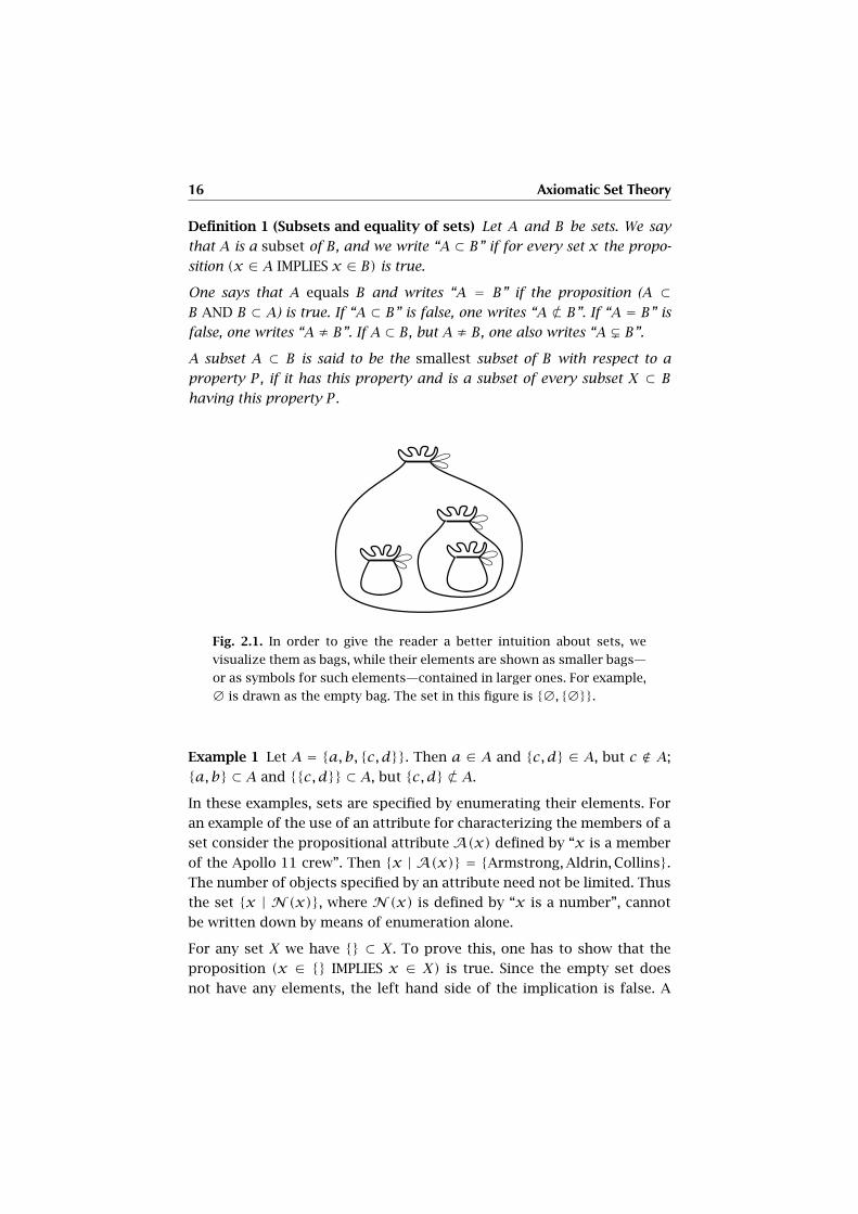
Example 3 The powerset of c = {a,b} is 2c = {∅, {a}, {b}, {a,b}}. If the
inclusion relation is drawn as an arrow from x to y if x ⊂ y then the
powerset of c can be illustrated as in figure 2.2.
{a,b}
∅
{a} {b}
Fig. 2.2. The powerset of {a,b}.
For the next axiom, one needs the following proposition:
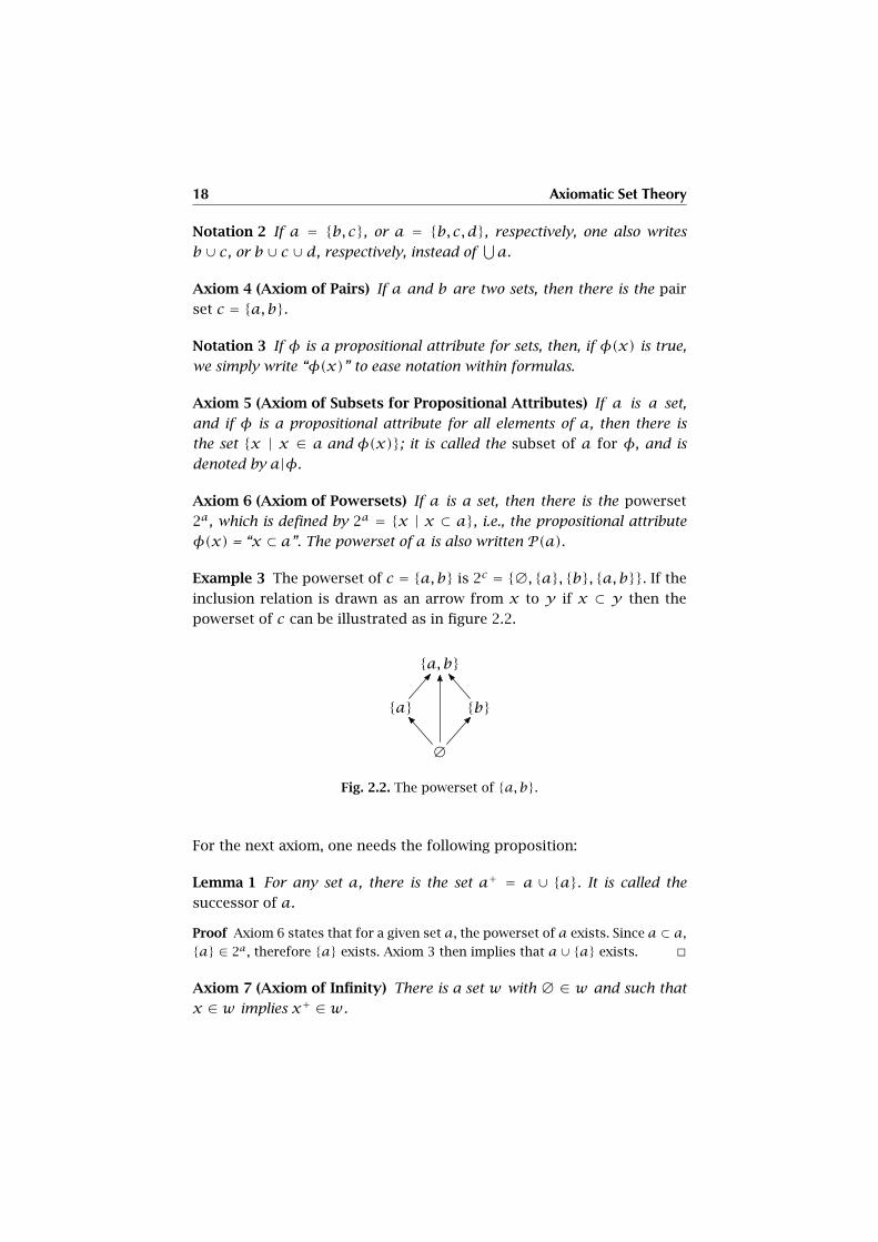
Lemma 1 For any set a, there is the set a+ = a ∪ {a}. It is called the
successor of a.
Proof Axiom 6 states that for a given set a, the powerset of a exists. Since a ⊂ a,
{a} ∈ 2a, therefore {a} exists. Axiom 3 then implies that a∪ {a} exists. �
Axiom 7 (Axiom of Infinity) There is a set w with ∅ ∈ w and such that
x ∈ w implies x+ ∈ w.
2.1 The Axioms 19
Fig. 2.3. The successor a+ of a set a.
Remark 1 Axiom 1 is a consequence of axioms 5 and 7, but we include
it, since axiom 7 is very strong (the existence of an infinite set is quite
hypothetical for a computer scientist).
Definition 2 For two sets a and b, the set {x | x ∈ a and x ∈ b} is called
the intersection of a and b and is denoted by a∩ b. If a∩ b = ∅, then a
and b are called disjoint.
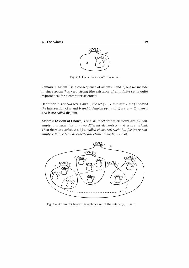
Axiom 8 (Axiom of Choice) Let a be a set whose elements are all non-
empty, and such that any two different elements x,y ∈ a are disjoint.
Then there is a subset c ⊂ ⋃a (called choice set) such that for every non-
empty x ∈ a, x ∩ c has exactly one element (see figure 2.4).
Fig. 2.4. Axiom of Choice: c is a choice set of the sets x, y , . . . ∈ a.
20 Axiomatic Set Theory
2.2 Basic Concepts and Results
We shall now develop the entire set theory upon these axioms. The be-
ginning is quite hard, but we shall be rewarded with a beautiful result:
all numbers from classical mathematics, all functions and all complex
structures will emerge from this construction.
Sorite 2 For any three sets a,b, c, we have
(i) a ⊂ a(ii) If a ⊂ b and b ⊂ a, then a = b.
(iii) If a ⊂ b and b ⊂ c, then a ⊂ c.Proof (i) If x ∈ a then, trivially, x ∈ a. (ii) This is true by definition 1. (iii) Let
x ∈ a. This implies x ∈ b, because a ⊂ b. Moreover, b ⊂ c implies x ∈ c. So,
x ∈ a implies x ∈ c for any x, and this means a ⊂ c by definition. �
Proposition 3 For any sets a,b, c, d:
(i) (Commutativity of unions) the set a∪ b exists and equals b ∪ a,
(ii) (Associativity of unions) the sets (a ∪ b) ∪ c and a ∪ (b ∪ c) exist
and are equal, we may therefore write a∪ b ∪ c instead,
(iii) (a ∪ b ∪ c) ∪ d and a ∪ (b ∪ c ∪ d) exist and are equal, we may
therefore write a∪ b ∪ c ∪ d instead.
Proof (i) By axiom 4 the set x = {a,b} exits. By axiom 3 both unions exist and we
have a ∪ b = ⋃x = {c | there is a m ∈ x such that c ∈ m} = {c | c ∈ a or c ∈b}. On the other hand, b∪a = ⋃y , where y = {b,a} = x, so the two unions are
equal.
(ii) (a ∪ b) ∪ c = {x | x ∈ a ∪ b} ∪ c = {x | x ∈ a ∪ b or x ∈ c} = {x | x ∈a or x ∈ b or x ∈ c}. On the other hand, a∪(b∪c) = {x | x ∈ a or x ∈ b∪c} ={x | x ∈ a or x ∈ b or x ∈ c}, so the two are equal.
(iii) follows from (ii) by replacing d with c and b with b ∪ c in the proof. �
Remark 2 The set whose elements are all sets x with x 6∈ x does not
exist, in fact both, the property x ∈ x, as well as x 6∈ x lead to contradic-
tions. Therefore, by axiom 5, the set of all sets does not exist.
Proposition 4 If a ≠ ∅, then the set {x | x ∈ z for all z ∈ a} exists, it is
called the intersection of a and is denoted by⋂a. However, for a = ∅,
the attribute Φ(x) = “x ∈ z for all z ∈ a” is fulfilled by every set x, and
therefore⋂∅ is inexistent, since it would be the non-existent set of all sets.
2.2 Basic Concepts and Results 21
Proof If a ≠ ∅, and if b ∈ a is one element satisfying the attribute Φ, the
required set is also defined by {x | x ∈ b and x ∈ z for all z ∈ a}. So this
attribute selects a subset of b defined by Φ, which is a legitimate set according
to axiom 5. If a = ∅, then the attribute Φ(x) alone is true for every set x, which
leads to the inexistent set of all sets. �
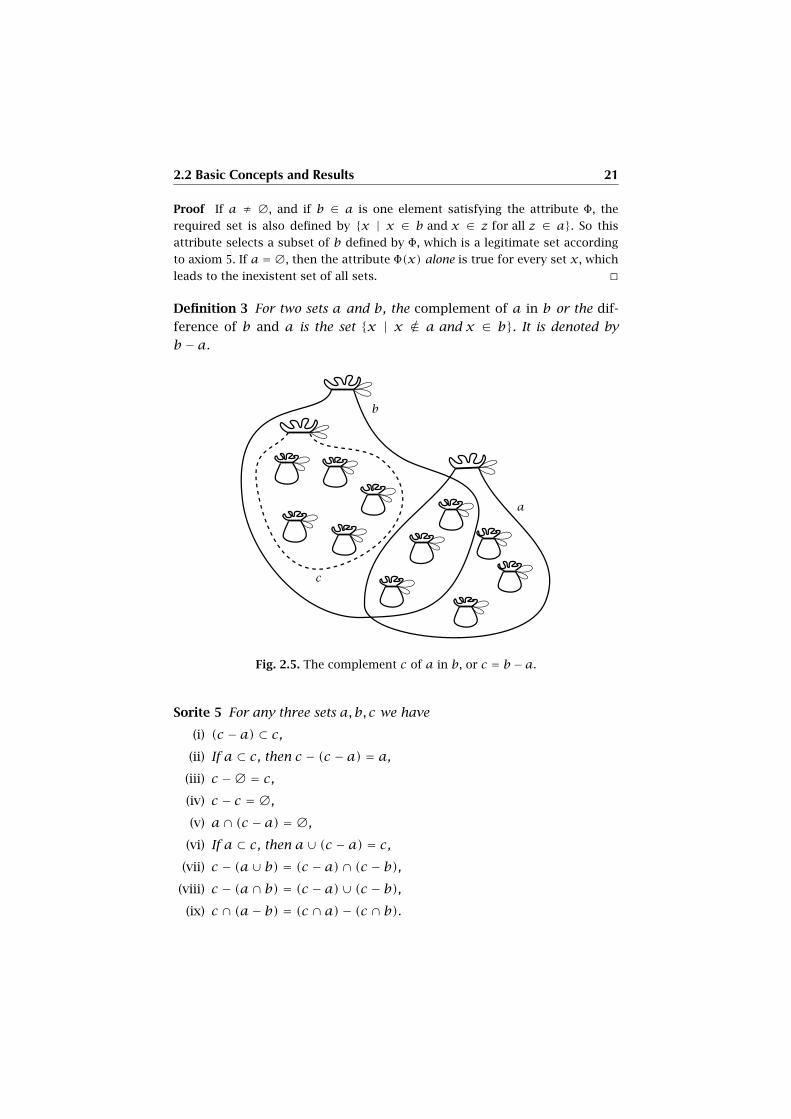
Definition 3 For two sets a and b, the complement of a in b or the dif-
ference of b and a is the set {x | x 6∈ a and x ∈ b}. It is denoted by
b − a.
Fig. 2.5. The complement c of a in b, or c = b − a.
Sorite 5 For any three sets a,b, c we have
(i) (c − a) ⊂ c,(ii) If a ⊂ c, then c − (c − a) = a,
(iii) c −∅ = c,(iv) c − c = ∅,
(v) a∩ (c − a) = ∅,
(vi) If a ⊂ c, then a∪ (c − a) = c,(vii) c − (a∪ b) = (c − a)∩ (c − b),
(viii) c − (a∩ b) = (c − a)∪ (c − b),(ix) c ∩ (a− b) = (c ∩ a)− (c ∩ b).
22 Axiomatic Set Theory
Proof We shall only prove part of the statements; the proof of the remaining
statements is left as an exercise for the reader.
(ii)
c − (c − a) = {x | x ∈ c and x 6∈ (c − a)}= {x | x ∈ c and not (x ∈ c and x 6∈ a)}= {x | x ∈ c and (x 6∈ c or not x 6∈ a)} (1)
= {x | x ∈ c and (x 6∈ c or x ∈ a)}= {x | (x ∈ c and x 6∈ c) or (x ∈ c and x ∈ a)} (2)
= {x | x ∈ c and x ∈ a} (3)
= {x | x ∈ a} (4)
= a
Equality (1) follows from de Morgan’s law, equality (2) from distributivity of
AND over OR. Equality (3) holds because the condition (x ∈ c and x 6∈ c) is
always false. Equality (4) holds because a ⊂ c means that x ∈ a already implies
x ∈ c, which therefore can be omitted. For the rules of transformation and
simplification used here, see also the discussion of truthtables on page 5.
(iv) By definition, c − c = {x | x ∈ c and x 6∈ c}. Obviously, there is no x which
can fulfill both of these contradictory conditions, so c − c = ∅.
(v)
a∩ (c − a) = {x | x ∈ a and x ∈ c − a}= {x | x ∈ a and (x ∈ c and x 6∈ a)}= {x | x ∈ a and x 6∈ a and x ∈ c} (∗)= ∅
Here we use the commutativity and associativity of AND to regroup and reorder
the terms of the propositional attribute. In line (∗) the attribute contains the
conjunction of a statement and its negation, which is always false, therefore the
result is the empty set.
(vii)
c − (a∪ b) = {x | x ∈ c and x 6∈ (a∪ b)}= {x | x ∈ c and not (x ∈ a or x ∈ b)}= {x | x ∈ c and (x 6∈ a and x 6∈ b)}= {x | x ∈ c and x 6∈ a and x 6∈ b} (1)
= {x | x ∈ c and x 6∈ a and x ∈ c and x 6∈ b} (2)
= {x | (x ∈ c and x 6∈ a) and (x ∈ c and x 6∈ b)} (3)
= {x | x ∈ c − a and x ∈ c − b} (4)
2.2 Basic Concepts and Results 23
= {x | x ∈ c − a} ∩ {x | x ∈ c − b} (5)
= (c − a)∩ (c − b)
Equalities (1) and (3) hold because AND is associative. Equality (2) holds be-
cause P AND Q = P AND P AND Q for any truth values P and Q. Equality (4) is
the definition of the set difference. Equality (5) is the definition of the intersec-
tion of two sets. �

CHAPTER 3
Boolean Set Algebra
In this chapter, we shall give a more systematic account of the construc-
tion of sets by use of union, intersection and complement. The structures
which emerge in this chapter are prototypes of algebraic structures which
will appear throughout the entire course.
3.1 The Boolean Algebra of Subsets
Lemma 6 For two sets a and b, the union a ∪ b is a least upper bound,
i.e., a,b ⊂ a∪b, and for every set c with a,b ⊂ c, we have a∪b ⊂ c. This
property uniquely determines the union.
Dually, the intersection a∩ b is a greatest lower bound, i.e., a∩ b ⊂ a,b,
and for every set c with c ⊂ a,b, we have c ⊂ a∩b. This property uniquely
determines the intersection.
Proof Clearly, a∪ b is a least upper bound. If x and y are any two least upper
bounds of a and b, then by definition, we must have x ⊂ y and y ⊂ x, therefore
x = y . The dual statement is demonstrated by analogous reasoning. �
Summarizing the previous properties of sets, we have the following im-
portant theorem, stating that the powerset 2a of a set a is a Boolean
algebra. We shall discuss this structure in a more systematic way in chap-
ter 17.
Proposition 7 (Boolean Algebra of Subsets) For a given set a, the power-
set 2a has the following properties. Let x,y, z be any elements of 2a, i.e.,
subsets of a; also, denote x′ = a− x. Then:
26 Boolean Set Algebra
(i) (Reflexivity) x ⊂ x,
(ii) (Antisymmetry) if x ⊂ y and y ⊂ x, then x = y ,
(iii) (Transitivity) if x ⊂ y and y ⊂ z, then x ⊂ z,
(iv) we have a “minimal” set ∅ ∈ 2a and a “maximal” set a ∈ 2a, and
∅ ⊂ x ⊂ a,
(v) (Least upper bound) the union x ∪y verifies x,y ⊂ x ∪y , and for
every z, if x,y ⊂ z, then x ∪y ⊂ z,
(vi) (dually: Greatest lower bound) the intersection x∩y verifies x∩y ⊂x,y , and for every z, if z ⊂ x,y , then z ⊂ x ∩y ,
(vii) (Distributivity) (x ∪ y) ∩ z = (x ∩ z) ∪ (y ∩ z) and (dually)
(x ∩y)∪ z = (x ∪ z)∩ (y ∪ z),(viii) we have x ∪ x′ = a, x ∩ x′ = ∅
Proof (i) is true for any set, see sorite 2.
(ii) is the very definition of equality of sets.
(iii) is immediate from the definition of subsets.
(iv) is clear.
(v) and (vi) were proved in lemma 6.
(vii) is clear.
(viii) follows immediately from the definition of the complement x′. �
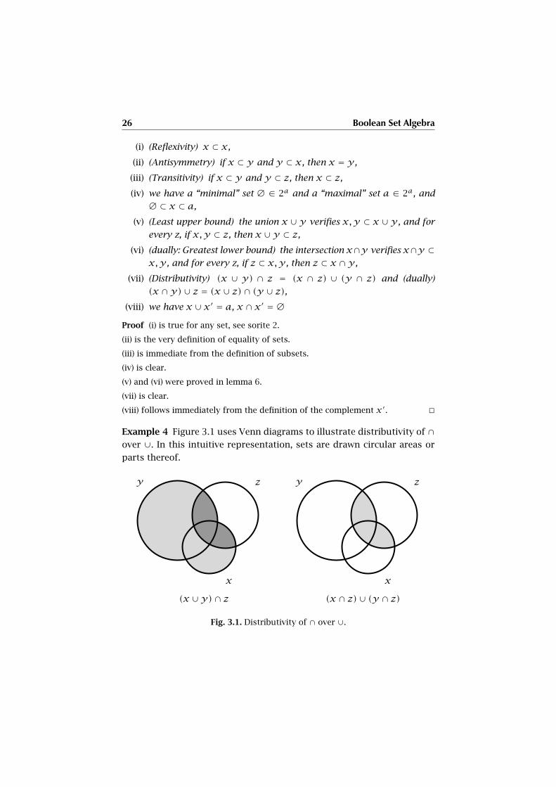
Example 4 Figure 3.1 uses Venn diagrams to illustrate distributivity of ∩over ∪. In this intuitive representation, sets are drawn circular areas or
parts thereof.
y z
x
(x ∪y)∩ z
y z
x
(x ∩ z)∪ (y ∩ z)
Fig. 3.1. Distributivity of ∩ over ∪.

3.1 The Boolean Algebra of Subsets 27
Exercise 1 Given a set a = {r , s, t} consisting of pairwise different sets,
give a complete description of 2a and the intersections or unions, respec-
tively, of elements of 2a.
Here is a second, also important structure on the powerset of a given set
a:
Definition 4 For x,y ∈ 2a, we define x + y = (x ∪ y) − (x ∩ y) (sym-
metric set difference). We further define x ·y = x∩y . Both operations are
illustrated using Venn diagrams in figure 3.2.
x y
x +y
x y
x ·y
Fig. 3.2. Symmetric difference and intersection of sets.
Proposition 8 For a set a, and for any three elements x,y, z ∈ 2a, we
have:
(i) (Commutativity) x +y = y + x and x ·y = y · x,
(ii) (Associativity) x + (y + z) = (x + y) + z, x · (y · z) = (x · y) · z,
we therefore also write x +y + z and x ·y · z, respectively,
(iii) (Neutral elements) we have x +∅ = x and x · a = x,
(iv) (Distributivity) x · (y + z) = x ·y + x · z,
(v) (Idempotency) x · x = x,
(vi) (Involution) x + x = ∅,
(vii) the equation x +y = z has exactly one solution w for the unknown
x, i.e., there is exactly one set w ⊂ a such that w +y = z.
Proof (i) follows from the commutativity of the union a∪b and the intersection
a∩ b, see also proposition 3.

28 Boolean Set Algebra
(ii) associativity also follows from associativity of union and intersection, see
again proposition 3.
(iii) we have x +∅ = (x ∪∅)− (x ∩∅) = x −∅ = x, x · a = x ∩ a = x.
(iv)
x · (y + z) = x ∩ ((y ∪ z)− (y ∩ z))= x ∩ (y ∪ z)− x ∩y ∩ z= ((x ∩y)∪ (x ∩ z))− x ∩y ∩ z
whereas
x ·y + x · z = ((x ∩y)∪ (x ∩ z))− ((x ∩y)∩ (x ∩ z))= ((x ∩y)∪ (x ∩ z))− x ∩y ∩ z
and we are done.
(v) and (vi) are immediate from the definitions.
(vii) in view of (vi),w = y+z is a solution. For any two solutionsw+y = w ′+y ,
one has w = w +y +y = w′ +y +y = w′. �
y z
x
x · (y + z)
y z
x
x ·y + x · z
Fig. 3.3. Distributivity of · over +.
Remark 3 This structure will later be discussed as the crucial algebraic
structure of a commutative ring, see chapter 15.
Exercise 2 Let a = {r , s, t} as in exercise 1. Calculate the solution of
w +y = z within 2a for y = {r , s} and z = {s, t}.
Exercise 3 Let a = {∅}. Calculate the complete tables of sums x+y and
products x · y , respectively, for x,y ∈ 2a, use the symbols 0 = ∅ and
1 = a. What do they remind you of?
CHAPTER 4
Functions and Relations
We have seen in chapter 1 that the conceptual architecture may be a se-
lection, conjunction, or disjunction. Sets are built on the selection type.
They are however suited for simulating the other types as well. More pre-
cisely, for the conjunction type, one needs to know the position of each
of two conceptual coordinates: Which is the first, which is the second. In
the selective type, however, no order between elements of a set is given,
i.e., {x,y} = {y,x}. So far, we have no means for creating order among
such elements. This chapter solves this problem in the framework of set
theory.
4.1 Graphs and Functions
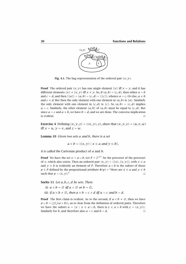
Definition 5 If x and y are two sets, the ordered pair (x,y) is defined to
be the following set:
(x,y) = {{x}, {x,y}}
Observe that the set (x,y) always exists, it is a subset of the powerset of
the pair set {x,y}, which exists according to axiom 4.
Here is the essence of this definition:
Lemma 9 For any four sets a,b, c, d, we have (a, b) = (c, d) iff a = c and
b = d. Therefore one may speak of the first and second coordinate a and
b, respectively, of the ordered pair (a, b).
30 Functions and Relations
Fig. 4.1. The bag representation of the ordered pair (x,y).
Proof The ordered pair (x,y) has one single element {x} iff x = y , and it has
different elements {x} ≠ {x,y} iff x ≠ y . So, if (a, b) = (c, d), then either a = band c = d, and then {{a}} = (a, b) = (c, d) = {{c}}, whence a = c. Or else, a ≠ b
and c ≠ d. But then the only element with one element in (a, b) is {a}. Similarly
the only element with one element in (c, d) is {c}. So (a, b) = (c, d) implies
a = c. Similarly, the other element {a,b} of (a, b) must be equal to {c,d}. But
since a = c and a ≠ b, we have b = d, and we are done. The converse implication
is evident. �
Exercise 4 Defining (x,y, z) = ((x,y), z), show that (x,y, z) = (u,v,w)iff x = u, y = v , and z = w.
Lemma 10 Given two sets a and b, there is a set
a× b = {(x,y) | x ∈ a and y ∈ b},
it is called the Cartesian product of a and b.
Proof We have the set v = a∪ b. Let P = 2(2v ) be the powerset of the powerset
of v , which also exists. Then an ordered pair (x,y) = {{x}, {x,y}}, with x ∈ aand y ∈ b is evidently an element of P . Therefore a × b is the subset of those
p ∈ P defined by the propositional attribute Φ(p) = “there are x ∈ a and y ∈ bsuch that p = (x,y).” �
Sorite 11 Let a,b, c, d be sets. Then:
(i) a× b = ∅ iff a = ∅ or b = ∅,
(ii) if a× b ≠∅, then a× b = c × d iff a = c and b = d.
Proof The first claim is evident. As to the second, if a × b ≠ ∅, then we have
a∪ b = ⋃(⋃(a× b)), as is clear from the definition of ordered pairs. Therefore
we have the subset a = {x | x ∈ a ∪ b, there is z ∈ a × b with z = (x,y)}.Similarly for b, and therefore also a = c and b = d. �
4.1 Graphs and Functions 31
a
b
(x,y)
x
y
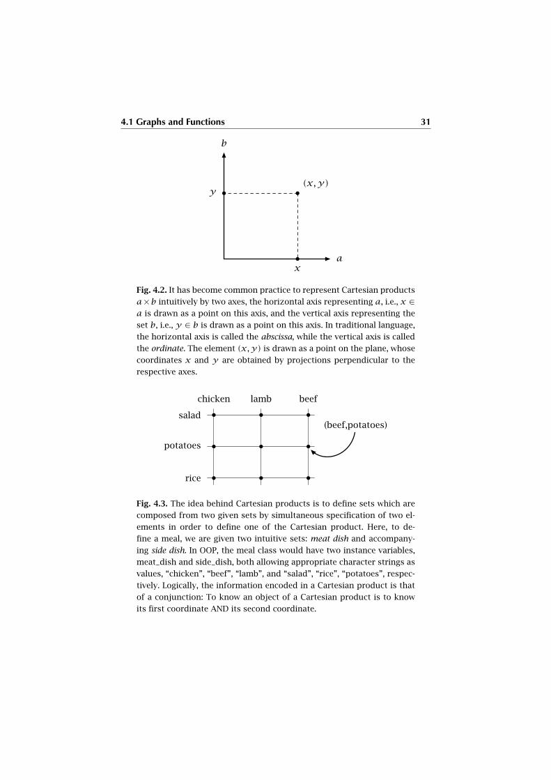
Fig. 4.2. It has become common practice to represent Cartesian products
a×b intuitively by two axes, the horizontal axis representing a, i.e., x ∈a is drawn as a point on this axis, and the vertical axis representing the
set b, i.e., y ∈ b is drawn as a point on this axis. In traditional language,
the horizontal axis is called the abscissa, while the vertical axis is called
the ordinate. The element (x,y) is drawn as a point on the plane, whose
coordinates x and y are obtained by projections perpendicular to the
respective axes.
chicken lamb beef
salad
potatoes
rice
(beef,potatoes)
Fig. 4.3. The idea behind Cartesian products is to define sets which are
composed from two given sets by simultaneous specification of two el-
ements in order to define one of the Cartesian product. Here, to de-
fine a meal, we are given two intuitive sets: meat dish and accompany-
ing side dish. In OOP, the meal class would have two instance variables,
meat_dish and side_dish, both allowing appropriate character strings as
values, “chicken”, “beef”, “lamb”, and “salad”, “rice”, “potatoes”, respec-
tively. Logically, the information encoded in a Cartesian product is that
of a conjunction: To know an object of a Cartesian product is to know
its first coordinate AND its second coordinate.

32 Functions and Relations
Definition 6 If a Cartesian product a×b is non-empty, we call the uniquely
determined sets a and b its first and second projection, respectively, and
we write a = pr1(a× b) and b = pr2(a× b).
The following concept of a graph is a formalization of the act of associ-
ating two objects out of two domains, such as the pairing of a man and a
woman, or associating a human and its bank accounts.
Lemma 12 The following statements about a set g are equivalent:
(i) The set g is a subset of a Cartesian product set a× b.
(ii) Every element x ∈ g is an ordered pair x = (u,v).Proof Clearly, (i) implies (ii). Conversely, if g consists of ordered pairs, we may
take P = ⋃(⋃g), and then immediately see that g ⊂ P × P . �
Definition 7 A set which satisfies one of the two equivalent properties of
lemma 12 is called a graph.
Example 5 For any set a, the diagonal graph is the graph
∆a = {(x,x) | x ∈ a}.
Lemma 13 For a graph g, there are two sets
pr1(g) = {u | (u,v) ∈ g} and pr2(g) = {v | (u,v) ∈ g},
and we have g ⊂ pr1(g)× pr2(g).
Proof As in the previous proofs, we take the double union P = ⋃(⋃g) and
from P extract the subsets pr1(g) and pr2(g) as defined in this proposition. The
statement g ⊂ pr1(g)× pr2(g) is then straightforward. �
Proposition 14 If g is a graph, there is another graph, denoted by g−1
and called the inverse graph of g, which is defined by
g−1 = {(v,u) | (u,v) ∈ g}.
We have (g−1)−1 = g.
Proof According to lemma 12, there are sets a and b such that g ⊂ a × b.
Then g−1 ⊂ b × a is the inverse graph. The statement about double inversion is
immediate. �

4.1 Graphs and Functions 33
b
apr1(g)
pr2(g)
g
pr1(g)× pr2(g)
Fig. 4.4. The projections pr1(g) and pr2(g) (dark gray segments on the
axes) of a graph g (black curves). Note that g ⊂ pr1(g) × pr2(g) (light
gray rectangles).
b
a
g−1
g
Fig. 4.5. The inverse g−1 of a graph g.
Exercise 5 Show that g = ∆pr1(g) implies g = g−1; give counterexamples
for the converse implication.
Definition 8 If g and h are two graphs, there is a set g◦h, the composition
of g with h (attention: the order of the graphs is important here), which is
defined by
g ◦ h = {(v,w) | there is a set u such that (v,u) ∈ h and (u,w) ∈ g}.
34 Functions and Relations
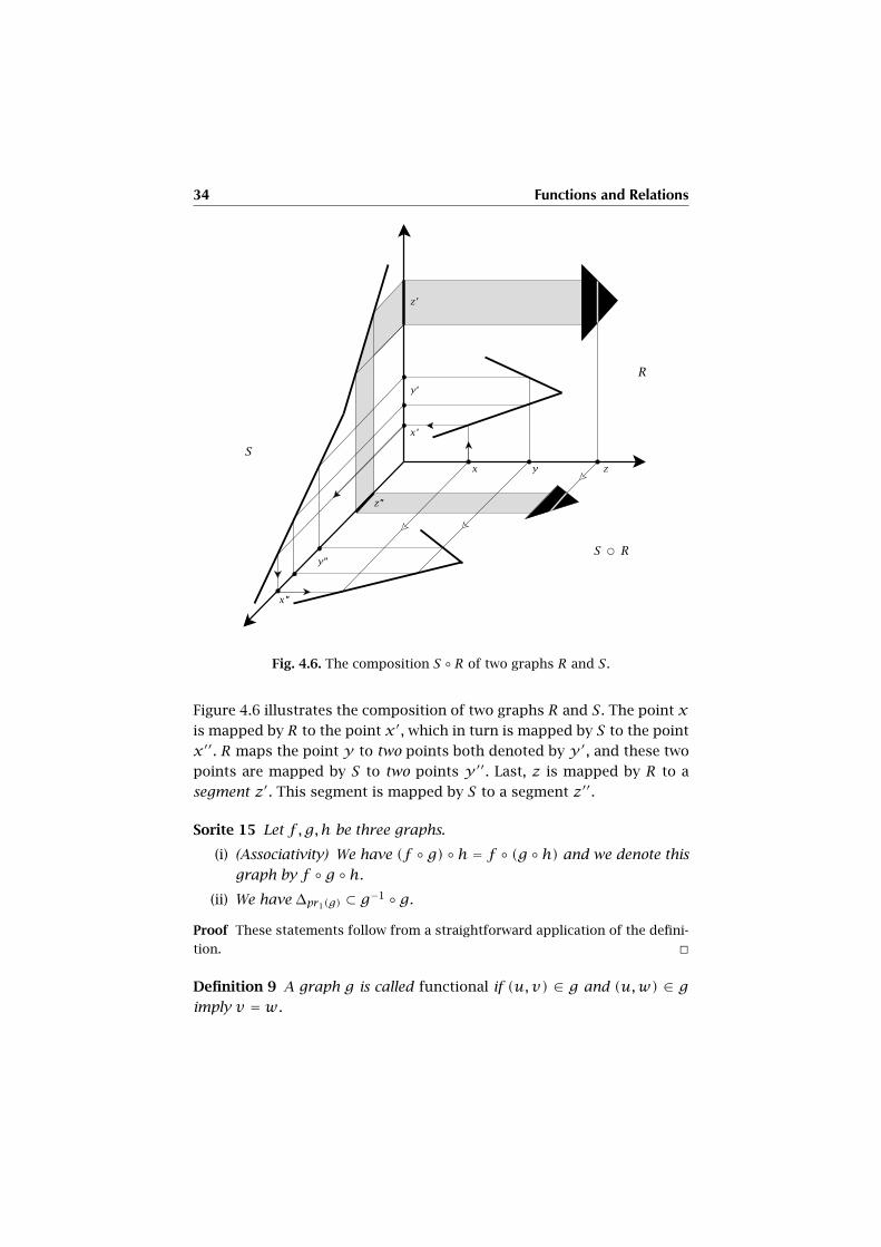
Fig. 4.6. The composition S ◦ R of two graphs R and S.
Figure 4.6 illustrates the composition of two graphs R and S. The point x
is mapped by R to the point x′, which in turn is mapped by S to the point
x′′. R maps the point y to two points both denoted by y ′, and these two
points are mapped by S to two points y ′′. Last, z is mapped by R to a
segment z′. This segment is mapped by S to a segment z′′.
Sorite 15 Let f , g,h be three graphs.
(i) (Associativity) We have (f ◦ g) ◦ h = f ◦ (g ◦ h) and we denote this
graph by f ◦ g ◦ h.
(ii) We have ∆pr1(g) ⊂ g−1 ◦ g.
Proof These statements follow from a straightforward application of the defini-
tion. �
Definition 9 A graph g is called functional if (u,v) ∈ g and (u,w) ∈ gimply v = w.
4.1 Graphs and Functions 35
Exercise 6 Show that the composition g ◦ h of two functional graphs g
and h is functional.
Example 6 For any sets a and b, the diagonal graph ∆a is functional,
whereas the Cartesian product a × b is not functional if a ≠ ∅ and if
there are sets x,y ∈ b with x ≠ y .
Definition 10 A function is a triple (a, f , b) such that f is a functional
graph, where a = pr1(f ) and pr2(f ) ⊂ b. The set a is called the domain
of the function, the set b is called its codomain, and the set pr2(f ) is called
the function’s image and denoted by Im(f ). One usually denotes a function
by a more graphical sign f : a→ b. For x ∈ a, the unique y ∈ b such that
(x,y) ∈ f is denoted by f(x) and is called the value of the function at the
argument x. Often, if the domain and codomain are clear, one identifies
the function with the graph sign f , but this is not the valid definition. One
then also notates a = dom(f ) and b = codom(f ).
Example 7 For any set a, the identity function (on a) Ida is defined by
Ida = (a,∆a, a).
Exercise 7 For the set 1 = {∅} and for any set a, show that there is
exactly one function (a, f ,1). We denote this function by ! : a → 1. (The
notation “1” is not quite arbitrary, we shall see the systematic background
in chapter 5.) If a = ∅, and if b is any set, show that there is a unique
function (∅, g, b), also denoted by ! :∅→ b.
Definition 11 A function f : a → b is called epimorphism, or epi, or
surjective or onto if Im(f ) = codom(f ).
It is called monomorphism, or mono, or injective or one-to-one if f(x) =f(y) implies x = y for all sets x,y ∈ dom(f ).
The function is called isomorphism, or iso, or bijective if it is epi and
mono. Isomorphisms are also denoted by special arrows, i.e., f : a∼→ b.
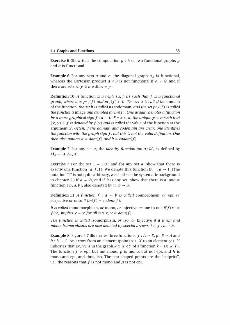
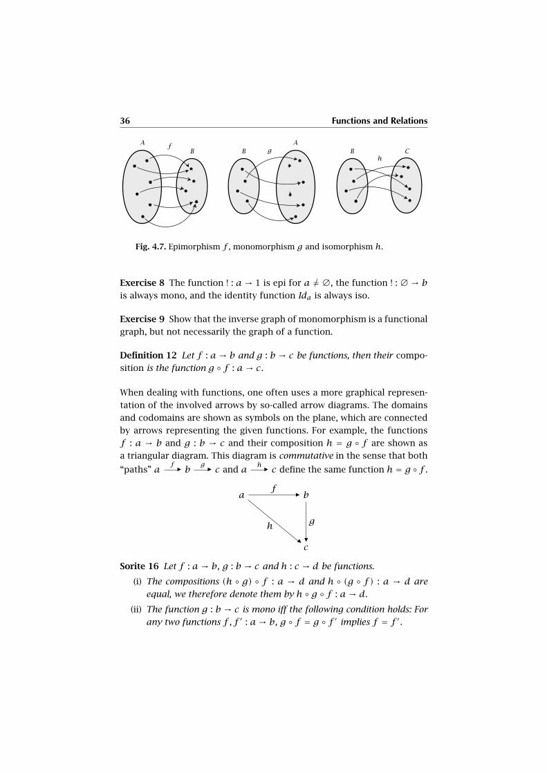
Example 8 Figure 4.7 illustrates three functions, f : A→ B, g : B → A and
h : B → C. An arrow from an element (point) x ∈ X to an element y ∈ Yindicates that (x,y) is in the graph κ ⊂ X×Y of a function k = (X, κ, Y).The function f is epi, but not mono, g is mono, but not epi, and h is
mono and epi, and thus, iso. The star-shaped points are the “culprits”,
i.e., the reasons that f is not mono and g is not epi.
36 Functions and Relations
Fig. 4.7. Epimorphism f , monomorphism g and isomorphism h.
Exercise 8 The function ! : a → 1 is epi for a 6= ∅, the function ! :∅ → bis always mono, and the identity function Ida is always iso.
Exercise 9 Show that the inverse graph of monomorphism is a functional
graph, but not necessarily the graph of a function.
Definition 12 Let f : a→ b and g : b → c be functions, then their compo-
sition is the function g ◦ f : a→ c.
When dealing with functions, one often uses a more graphical represen-
tation of the involved arrows by so-called arrow diagrams. The domains
and codomains are shown as symbols on the plane, which are connected
by arrows representing the given functions. For example, the functions
f : a → b and g : b → c and their composition h = g ◦ f are shown as
a triangular diagram. This diagram is commutative in the sense that both
“paths” afñ b
gñ c and a
hñ c define the same function h = g ◦ f .
af
ñ b
c
g
�
h
ñ
Sorite 16 Let f : a→ b, g : b → c and h : c → d be functions.
(i) The compositions (h ◦ g) ◦ f : a → d and h ◦ (g ◦ f) : a → d are
equal, we therefore denote them by h ◦ g ◦ f : a→ d.
(ii) The function g : b → c is mono iff the following condition holds: For
any two functions f , f ′ : a→ b, g ◦ f = g ◦ f ′ implies f = f ′.
4.1 Graphs and Functions 37
(iii) The function f : a → b is epi iff the following condition holds: For
any two functions g,g′ : b → c, g ◦ f = g′ ◦ f implies g = g′.(iv) If f and g are epi, mono, iso, respectively, then so is g ◦ f .
(v) If f is mono and a ≠ ∅, then there is a—necessarily epi—function
r : b → a such that r ◦ f = Ida, such a function is called a left
inverse or retraction of f .
(vi) If f is epi, then there is a—necessarily mono—function s : b → a
such that f ◦ s = Idb, such a function is called a right inverse or
section of f .
(vii) The function f is iso iff there is a (necessarily unique) inverse, de-
noted by f−1 : b → a, such that f−1 ◦ f = Ida and f ◦ f−1 = Idb.
Proof (i) follows from the associativity of graph composition, see sorite 15.
(ii) For x ∈ a, (g ◦ f)(x) = (g ◦ f ′)(x) means g(f(x)) = g(f ′(x)), but since g
is mono, f(x) = f ′(x), for all x ∈ a, whence f = f ′. Conversely, take u,v ∈ bsuch that g(u) = g(v). Define two maps f , f ′ : 1→ b by f(0) = u and f ′(0) = v .
Then g ◦ f = g ◦ f ′. So f = f ′, but this means u = f(0) = f ′(0) = v , therefore
g is injective.
(iii) If f is epi, then for every y ∈ b, there is x ∈ a with y = f(x). If g◦f = g′◦f ,
then g(y) = g(f(x)) = g′(f (x)) = g′(y), whence g = g′. Conversely, if f is
not epi, then let z 6∈ Im(f ). Define a function g : b → {0,1} by g(y) = 0 for all
y ∈ b. Define g′ : b → {0,1} by g′(y) = 0 for all y ≠ z, and g′(z) = 1. We then
have two different functions g and g′ such that g ◦ f = g′ ◦ f .
(iv) This property follows elegantly from the previous characterization: let f and
g be epi, then for h,h′ : c → d, if h ◦ g ◦ f = h′ ◦ g ◦ f , then, since f is epi, we
conclude h ◦ g = h′ ◦ g, and since g is epi, we have h = h′. The same formal
argumentation works for mono. Since iso means mono and epi, we are done.
(v) If f : a → b is mono, then the inverse graph f−1 is also functional and
pr2(f−1) = a. Take any element y ∈ a and take the graph r = f −1 ∪ (b −
Im(f ))× {y}). This defines a retraction of f .
(vi) Let f be epi. For every x ∈ b, let F(x) = {y | y ∈ a, f (y) = x}. Since f is
epi, no F(x) is empty, and F(x)∩ F(x′) = ∅ if x ≠ x′. By the axiom of choice 8,
there is a set q ⊂ a such that q ∩ F(x) = {qx} is a set with exactly one element
qx for every x ∈ b. Define s(x) = qx . This defines the section s : b → a of f .
(vii) The case a = ∅ is trivial, so let us suppose a ≠ ∅. Then the characteri-
zations (v) and (vi), together with the fact that “mono + epi = iso”, answer our
problem. �
Remark 4 The proof of statement (vi) in sorite 16 is a very strong one
since it rests on the axiom of choice 8.
38 Functions and Relations
Definition 13 Let f : a → b be a function, and let a′ be a set. Then the
restriction of f to a′ is the function f |a′ : a∩ a′ → b, where the graph is
f |a′ = f ∩ ((a∩ a′)× b).
Definition 14 Let f : a → b and g : c → d be two functions. Then the
Cartesian product of f and g is the function f × g : a × c → b × d with
(f × g)(x,y) = (f (x), g(y)).
Sorite 17 Let f : a→ b and g : c → d be two functions. Then the Cartesian
product f × g is injective (surjective, bijective) if f and g are so.
Proof If one of the domains a or c is empty the claims are obvious. So suppose
a, c ≠∅. Let f and g be injective and take two elements (x,y) ≠ (x′, y ′) in a×b.
Then either x ≠ x′ or y ≠ y ′. in the first case, (f × g)(x,y) = (f (x), g(y)) ≠(f (x′), g(y)) = (f ×g)(x′, y), the second case is analogous. A similar argument
settles the cases of epi maps, and the case of iso maps is just the conjunction of
the mono and epi cases. �
The next subject is the basis of the classification of sets. The question is:
When are two sets “essentially different”? This is the crucial definition:
Definition 15 A set a is said to be equipollent to b or to have the same
cardinality as b iff there is a bijection f : a∼→ b. We often just write a
∼→ bto indicate the fact that a and b are equipollent.
Example 9 In figure 4.8, the set A of stars, the set B of crosses and the
set C of plusses are equipollent. The functions f : A → B and g : B → Care both bijections. The composition of g and f is a bijection h = g ◦ f :
A → C. The purpose of this example is to show that equipollence is a
feature independent of the shape, or “structure” of the set. It only tells
us that each element from the first set can be matched with an element
from the second set, and vice-versa.
Proposition 18 For all sets a, b and c, we have:
(i) (Reflexivity) a is equipollent to a.
(ii) (Symmetry) If a is equipollent to b, then b is equipollent to a.
(iii) (Transitivity) If a is equipollent to b, and if b is equipollent to c, then
a is equipollent to c.
Proof Reflexivity follows from the fact that the identity Ida is a bijection. Symme-
try follows from statement (vii) in sorite 16. Transitivity follows from statement
(iv) of sorite 16. �

4.1 Graphs and Functions 39
6 6 6 6 6 6 6 6 6 6 6 6
H H H H
H H H H
H H H H
: : :
: : :
: : :
: : :
B(6)
A(H)
C(:)
f
g
Fig. 4.8. The equipollence of sets A, B and C .
Are there arbitrary large sets? Here are first answers:
Exercise 10 Show that there is an injection sing : a → 2a for each set a,
defined by sing(x) = {x}.
An injection in the reverse direction never exists. We have in fact this
remarkable theorem.
Proposition 19 For any set a, a and 2a are never equipollent.
Proof Suppose that we have a function f : a → 2a. We show that f cannot be
surjective. Take the subset g ⊂ a defined by g = {x | x ∈ a,x 6∈ f(x)}. We claim
that g 6∈ Im(f ). If z ∈ a with f(z) = g, then if z 6∈ g, then z ∈ g, a contradiction.
But if z ∈ g, then z 6∈ f(z) by definition of g, again a contradiction. So f(z) = gis impossible. �
To see why this contradicts the existence of an injection 2a → a, we need
some further results:
Sorite 20 Let a,b, c, d be sets.
(i) If a∼→ b and c
∼→ d, then a× c ∼→ b × d.
(ii) If a∼→ b and c
∼→ d, and if a∩ c = b ∩ d = ∅, then a∪ c ∼→ b ∪ d.
Proof (i) If f : a→ b and g : c → d are bijections, then so is f × g by sorite 17.
(ii) If f : a→ b and g : c → d are bijections, then the graph f∪g ⊂ (a∪c)×(b∪d)clearly defines a bijection. �
40 Functions and Relations
The following is a technical lemma:
Lemma 21 If p ∪ q ∪ r ∼→ p and p ∩ q = ∅, then p ∪ q ∼→ p.
Proof This proof is more involved and should be read only by those who really
are eager to learn about the innards of set theory. To begin with, fix a bijection
f : p ∪ q ∪ r → p. If x ⊂ p ∪ q ∪ r , we also write f(x) for {f(z) | z ∈ x}.Consider the following propositional attribute Ψ(x) of elements x ∈ 2p∪q∪r : We
define Ψ(x) = “q∪f(x) ⊂ x”. For example, we have Ψ(p∪q). We now show that
if Ψ(x), then also Ψ(q∪f(x)). In fact, if q∪f(x) ⊂ x, then f(q∪f(x)) ⊂ f(x),and a fortiori f(q ∪ f(x)) ⊂ q ∪ f(x), therefore q ∪ f(q ∪ f(x)) ⊂ q ∪ f(x),thus Ψ(q ∪ f(x)), therefore Ψ(k).
Next, let b ⊂ 2p∪q∪r with Ψ(x) for all x ∈ b. Now we show that Ψ(⋂b). Denote
k = ⋂b. Since k ⊂ x for all x ∈ b, we also have f(k) ⊂ f(x) for all x ∈ b, and
therefore q ∪ f(k) ⊂ q ∪ f(x) ⊂ x for all x ∈ b. This implies q ∪ f(k) ⊂ k.
Now let b = e = {x | x ∈ 2p∪q∪r and Ψ(x)}; we know that e is non-empty. Then
k = d = ⋂ e. From the discussion above, it follows that Ψ(d), i.e., q ∪ f(d) ⊂ d.
But by the first consideration, we also know that Ψ(q∪f(d)), and, since d is the
intersection of all x such that Ψ(x), d ⊂ q ∪ f(d). This means that q ∪ f(d) ⊂d ⊂ q ∪ f(d), i.e., q ∪ f(d) = d.
Moreover, d∩(p−f(d)) = ∅. In fact, d∩(p−f(d)) = (q∪f(d))∩(p−f(d)) =(q∩(p−f(d)))∪(f (d)∩(p−f(d))) = ∅∪∅ = ∅ because we suppose p∩q = ∅.
So we have a disjoint union q ∪ p = d ∪ (p − f(d)). Now, we have a bijection
f : d∼→ f(d) and a bijection (the identity) p − f(d) ∼→ p − f(d). Therefore by
sorite 20 (ii), we obtain the required bijection. �
This implies a famous theorem:
Proposition 22 (Bernstein-Schröder) Let a,b, c be three sets such that
there exist two injections f : a → b and g : b → c. If a and c are equipol-
lent, then all three sets are equipollent.
Proof We apply lemma 21 as follows. Let f : a → b and g : b → c be injections
and h : a → c a bijection. Then we may take the image sets a′ = g(f(a)) and
b′ = g(b) instead of the equipollent sets a and b, respectively. Therefore without
loss of generality we may show the theorem for the special situation of subsets
a ⊂ b ⊂ c such that a is equipollent to c. To apply our technical lemma we set
p = a, q = b − a and r = c − b. Therefore c = p ∪ q ∪ r and b = p ∪ q. In these
terms, we are supposing that p is equipollent to p∪ q∪ r . Therefore the lemma
yields that p is equipollent to p ∪ q, i.e., a is equipollent to b. By transitivity of
equipollence, b and c are also equipollent. �
In particular:
4.2 Relations 41
Corollary 23 If a ⊂ b ⊂ c, and if a is equipollent to c, then all three sets
are equipollent.
Corollary 24 For any set a, there is no injection 2a → a.
Proof If we had an injection 2a → a, the existing reverse injection a → 2a
from exercise 10 and proposition 22 would yield a bijection a∼→ 2a which is
impossible according to proposition 19. �
4.2 Relations
Until now, we have not been able to deal with “relations” in a formal
sense. For example, the properties of reflexivity, symmetry, and transitiv-
ity, as encountered in proposition 18, are only properties of single pairs
of sets, but the whole set of all such pairs is not given. The theory of
relations will deal with such problems.
Definition 16 A binary relation on a set a is a subset R ⊂ a × a; this is a
special graph, where the domain and codomain coincide and are specified
by the choice of a. Often, instead of “(x,y) ∈ R”, one writes “xRy”.
Example 10 The empty relation ∅ ⊂ a × a, the complete relation R =a × a, and the diagonal graph ∆a are relations on a. For each relation R
on a, the inverse relation R−1 = {(y,x) | (x,y) ∈ R} (the inverse graph)
is a relation on a. If R and S are two relations on a, then the composed
graph R ◦S defines the composed relation on a. In particular, we have the
second power R2 = R ◦ R of a relation R.
Notation 4 Often, relation symbols are not letters, but special symbols
such as <,≤,≺, . . . . Their usage is completely dependent on context and
has no universal meaning. Given relations < and ≤, the corresponding
inverse relations are denotated by > and ≥, respectively.
Definition 17 Let ≤ be a relation on a. The relation is called
(i) reflexive iff x ≤ x for all x ∈ a;
(ii) transitive iff x ≤ y and y ≤ z implies x ≤ z for all x,y, z ∈ a;
(iii) symmetric iff x ≤ y implies y ≤ x for all x,y ∈ a;
(iv) antisymmetric iff x ≤ y and y ≤ x implies x = y for all x,y ∈ a;
(v) total iff for any two x,y ∈ a, either x ≤ y or y ≤ x.
42 Functions and Relations
(vi) equivalence relation, iff it is reflexive, symmetric, and transitive. In
this case, the relation is usually denoted by ∼ instead of ≤.
Example 11 We shall illustrate these properties with examples from the
real world. The relation “x is an ancestor of y” is transitive, but neither
reflexive nor symmetric. The “subclass” relation of object-oriented pro-
gramming is reflexive, transitive, antisymmetric, but not symmetric.
The relation “x lives within 10 kilometers from y” is reflexive, symmetric,
but not transitive.
The relation “x is a sibling of y” is symmetric and transitive. It is not
reflexive. None of these relations is total.
A total, transitive relation, is, for instance, “x is not taller than y”.
Definition 18 Given a binary relation R ⊂ X × X, we call the smallest
set Rr , such that R ⊂ Rr and Rr is reflexive, the reflexive closure of R.
The smallest set Rs , such that R ⊂ Rs and Rs is symmetric, is called the
symmetric closure of R. The smallest set Rt , such that R ⊂ Rt and Rt is
transitive, is called the transitive closure of R. Finally, the smallest equiva-
lence relation Re containing R is called the equivalence relation generated
by R.
Proposition 25 If ∼ is an equivalence relation on a, and if s ∈ a, then a
subset
[s] = {r | r ∈ a and s ∼ r}is called an equivalence class with respect to ∼. The set of equivalence
classes—a subset of 2a—is denoted by a/∼. It defines a partition of a, i.e.,
for any two elements s, t ∈ a, either [s] = [t] or [s] ∩ [t] = ∅, and
a = ⋃(a/∼).Proof Since for every s ∈ a, s ∼ s, we have s ∈ [s], whence a = ⋃
(a/∼). If
u ∈ [s]∩ [t], then if r ∼ s we have r ∼ s ∼ u ∼ t, whence [s] ⊂ [t], the converse
inclusion holds with the roles of s and t interchanged, so [s] = [t]. �
Example 12 For an equivalence relation, consider “x has the same gen-
der as y”. The set of equivalence classes of this relation partitions
mankind into two sets, the set of males and the set of females.
Exercise 11 Show that the reflexive, symmetric, transitive closure ((Rr )s)tof a relation R is the smallest equivalence relation Re containing R. Hint:
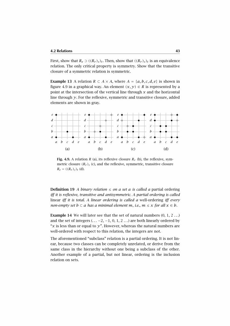
4.2 Relations 43
First, show that Re ⊃ ((Rr )s)t . Then, show that ((Rr )s)t is an equivalence
relation. The only critical property is symmetry. Show that the transitive
closure of a symmetric relation is symmetric.
Example 13 A relation R ⊂ A × A, where A = {a,b, c, d, e} is shown in
figure 4.9 in a graphical way. An element (x,y) ∈ R is represented by a
point at the intersection of the vertical line through x and the horizontal
line through y . For the reflexive, symmetric and transitive closure, added
elements are shown in gray.
a
a
b
b
c
c
d
d
e
e
(a)
a
a
b
b
c
c
d
d
e
e
(b)
a
a
b
b
c
c
d
d
e
e
(c)
a
a
b
b
c
c
d
d
e
e
(d)
Fig. 4.9. A relation R (a), its reflexive closure Rr (b), the reflexive, sym-
metric closure (Rr )s (c), and the reflexive, symmetric, transitive closure
Re = ((Rr )s)t (d).
Definition 19 A binary relation ≤ on a set a is called a partial ordering
iff it is reflexive, transitive and antisymmetric. A partial ordering is called
linear iff it is total. A linear ordering is called a well-ordering iff every
non-empty set b ⊂ a has a minimal element m, i.e., m ≤ x for all x ∈ b.
Example 14 We will later see that the set of natural numbers (0, 1, 2 . . .)
and the set of integers (. . . −2, −1, 0, 1, 2 . . .) are both linearly ordered by
“x is less than or equal to y”. However, whereas the natural numbers are
well-ordered with respect to this relation, the integers are not.
The aforementioned “subclass” relation is a partial ordering. It is not lin-
ear, because two classes can be completely unrelated, or derive from the
same class in the hierarchy without one being a subclass of the other.
Another example of a partial, but not linear, ordering is the inclusion
relation on sets.
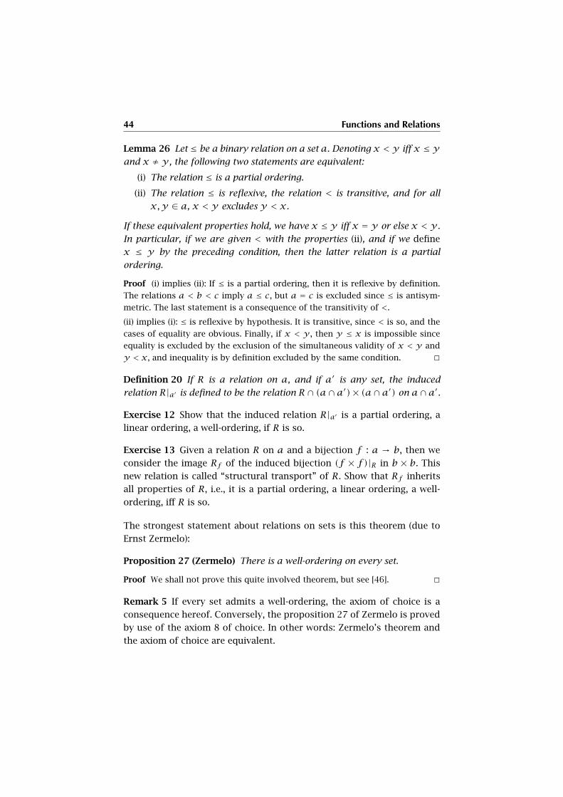
44 Functions and Relations
Lemma 26 Let ≤ be a binary relation on a set a. Denoting x < y iff x ≤ yand x ≠ y , the following two statements are equivalent:
(i) The relation ≤ is a partial ordering.
(ii) The relation ≤ is reflexive, the relation < is transitive, and for all
x,y ∈ a, x < y excludes y < x.
If these equivalent properties hold, we have x ≤ y iff x = y or else x < y .
In particular, if we are given < with the properties (ii), and if we define
x ≤ y by the preceding condition, then the latter relation is a partial
ordering.
Proof (i) implies (ii): If ≤ is a partial ordering, then it is reflexive by definition.
The relations a < b < c imply a ≤ c, but a = c is excluded since ≤ is antisym-
metric. The last statement is a consequence of the transitivity of <.
(ii) implies (i): ≤ is reflexive by hypothesis. It is transitive, since < is so, and the
cases of equality are obvious. Finally, if x < y , then y ≤ x is impossible since
equality is excluded by the exclusion of the simultaneous validity of x < y and
y < x, and inequality is by definition excluded by the same condition. �
Definition 20 If R is a relation on a, and if a′ is any set, the induced
relation R|a′ is defined to be the relation R∩ (a∩a′)× (a∩a′) on a∩a′.
Exercise 12 Show that the induced relation R|a′ is a partial ordering, a
linear ordering, a well-ordering, if R is so.
Exercise 13 Given a relation R on a and a bijection f : a → b, then we
consider the image Rf of the induced bijection (f × f)|R in b × b. This
new relation is called “structural transport” of R. Show that Rf inherits
all properties of R, i.e., it is a partial ordering, a linear ordering, a well-
ordering, iff R is so.
The strongest statement about relations on sets is this theorem (due to
Ernst Zermelo):
Proposition 27 (Zermelo) There is a well-ordering on every set.
Proof We shall not prove this quite involved theorem, but see [46]. �
Remark 5 If every set admits a well-ordering, the axiom of choice is a
consequence hereof. Conversely, the proposition 27 of Zermelo is proved
by use of the axiom 8 of choice. In other words: Zermelo’s theorem and
the axiom of choice are equivalent.
CHAPTER 5
Ordinal and Natural Numbers
Until now, our capabilities to produce concrete sets were quite limited.
In particular, we were only capable of counting from zero to one: from
the empty set 0 = ∅ to the set 1 = {0}. We are not even able to say
something like: “For n = 0,1, . . .”, since the dots have no sense up to
now! This serious lack will be abolished in this chapter: We introduce the
basic construction of natural numbers—together with one of the most
powerful proof techniques in mathematics: proof by infinite induction.
5.1 Ordinal Numbers
We shall now construct the basic sets needed for every counting and
number-theoretic task in mathematics (and all the sciences, which count
on counting, be aware of that!)
Definition 21 A set a is called transitive if x ∈ a implies x ⊂ a.
Example 15 The sets 0 and 1 are trivially transitive, and so is any set
J = {J} (if it exists).
Exercise 14 Show that if a and b are transitive, then so is a∩ b.
Definition 22 A set a is called alternative if for any two elements x,y ∈ a,
either x = y , or x ∈ y , or y ∈ x.
Exercise 15 Show that, if a is alternative and b ⊂ a, then b is alternative.
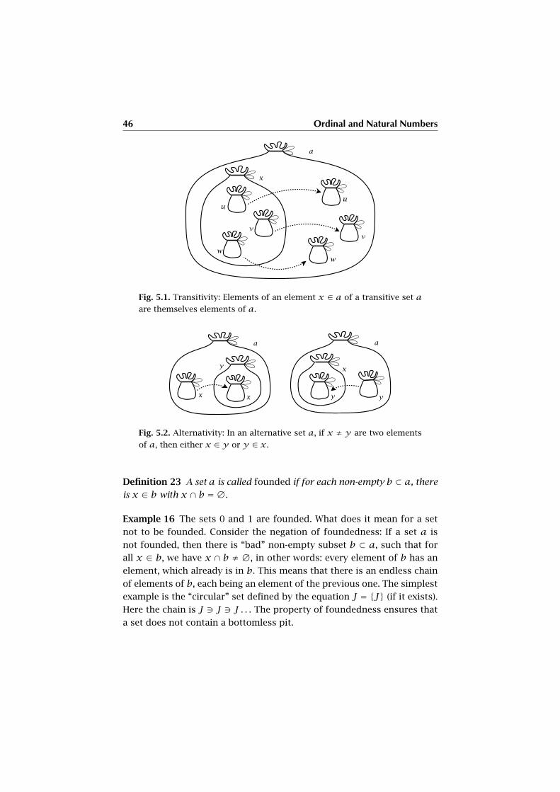
46 Ordinal and Natural Numbers
Fig. 5.1. Transitivity: Elements of an element x ∈ a of a transitive set a
are themselves elements of a.
Fig. 5.2. Alternativity: In an alternative set a, if x ≠ y are two elements
of a, then either x ∈ y or y ∈ x.
Definition 23 A set a is called founded if for each non-empty b ⊂ a, there
is x ∈ b with x ∩ b = ∅.
Example 16 The sets 0 and 1 are founded. What does it mean for a set
not to be founded. Consider the negation of foundedness: If a set a is
not founded, then there is “bad” non-empty subset b ⊂ a, such that for
all x ∈ b, we have x ∩ b ≠ ∅, in other words: every element of b has an
element, which already is in b. This means that there is an endless chain
of elements of b, each being an element of the previous one. The simplest
example is the “circular” set defined by the equation J = {J} (if it exists).
Here the chain is J 3 J 3 J . . . The property of foundedness ensures that
a set does not contain a bottomless pit.

5.1 Ordinal Numbers 47
Fig. 5.3. Foundedness: If b ⊂ a is non-empty, and a is founded, then
there is x ∈ b such that x ∩ b = ∅; here we have x = {r , s}, b ={x,u,v,w} with r ≠ u,v,w and s ≠ u,v,w.
In modern computer science, however, such circular sets play an increas-
ingly important role, a prominent example being the modeling of circular
data structures, see [3].
The circular non-founded set is a special case of the following result:
Proposition 28 Suppose that a is founded, then x ∈ a implies x 6∈ x.
Proof For x ∈ a, consider the subset {x} ⊂ a. Then x ∈ x contradicts the fact
that {x} ∩ x must be empty because a is founded. �
Lemma 29 If d is founded, and if a,b, c ∈ d such that a ∈ b and b ∈ c,then a ≠ c and c 6∈ a.
Proof Consider the subset {a,b} ∈ d. If x = b, then a ∈ x ∩ {a,b}. Therefore
x = a yields x ∩ {a,b} = ∅. But a = c enforces that b is in this intersection.
Therefore a ≠ c. If we had c ∈ a, then we cannot have a∩ {a,b, c} = ∅. By the
hypothesis of the lemma, b ∩ {a,b, c} contains a, and c ∩ {a,b, c} contains b.
Therefore the set {a,b, c} contradicts the foundedness of d and so c 6∈ a. �
Here is the fundamental concept for creating numbers:
Definition 24 A set is called ordinal if it is transitive, alternative, and
founded.
The following series of results is destined to control the basic properties
of ordinals.
48 Ordinal and Natural Numbers
Lemma 30 Let d be an ordinal. If a ⊂ d is non-empty, then there is x0 ∈ asuch that whenever x ∈ a, then either x0 = x or x0 ∈ x.
Proof Since d is an ordinal, it is founded, and there is an element x0 ∈ a such
that x0∩a = ∅. Let x ∈ a be any element different from x0. Since d is alternative,
either x ∈ x0 or x0 ∈ x. But x ∈ x0 contradicts x0 ∩ a = ∅, and we are done. �
Proposition 31 If d is ordinal, then x ∈ d implies that x is ordinal.
Proof Let x ∈ d. Then by transitivity of d, x ⊂ d. Hence x is alternative and
founded. Let b ∈ x. Then a ∈ b implies a ∈ x. In fact, x ⊂ d, therefore b ∈ dand a ∈ b ∈ d. Since d is transitive, a ∈ d. So a,x ∈ d. Hence either a = x, or
a ∈ x, or x ∈ a. But by lemma 29, applied to the element chain a ∈ b ∈ x, we
must have a ∈ x. �
Proposition 32 A transitive proper subset c of an ordinal d is an element
of that ordinal.
Proof Since d is founded, there is y ∈ d− c with y ∩ (d− c) = ∅. We claim that
c = y . Since d is transitive, y ⊂ d, and by construction of y , y ⊂ c. Conversely,
let b ∈ c, then b ∈ d. Since d is alternative, either b ∈ y or b = y or y ∈ b. But
b = y implies b ∈ d− c, a contradiction. Further, y ∈ b and b ∈ c imply y ∈ cby transitivity of c. Again, a contradiction. Therefore we have b ∈ y . �
Corollary 33 If d is an ordinal, then a set a is an element of d iff it is an
ordinal and a ⊊ d.
Proof Clearly, an element of an ordinal is a proper subset. The converse follows
from proposition 32. �
Exercise 16 Show that if d is a non-empty ordinal, then ∅ ∈ d.
Exercise 17 Show that if c is ordinal, then a ∈ b and b ∈ c imply a ∈ c.
Exercise 18 Show that if a and b are ordinals, then a ∈ b implies b 6∈ a.
Proposition 34 If a and b are ordinals, then either a ⊂ b or b ⊂ a.
Proof Suppose both conclusions are wrong. Then the intersection a ∩ b is a
proper subset of both a and b. But it is evidently transitive, hence an ordinal
element of both, a and b, hence an element of itself, a contradiction. �
Corollary 35 If a and b are ordinals, then exclusively either a ∈ b, or
a = b, or b ∈ a.
5.1 Ordinal Numbers 49
Proof Follows from propositions 32 and 34. �
Corollary 36 If all elements a ∈ b are ordinals, then b is alternative.
Proof Follows from corollary 35. �
Proposition 37 If every element x ∈ u of a set u is ordinal, then there
is exactly one element x0 ∈ u such that for every x ∈ u, we have either
x0 ∈ x or x0 = x.
Proof Uniqueness is clear since all elements of u are ordinal.
Existence: If u = {a}, then take x0 = a. Else, there are at least two different
elements c, c′ ∈ u, and either c ∈ c′ or c′ ∈ c. So either c ∩ u or c′ ∩ u is not
empty. Suppose c ∩u ≠∅. By lemma 30, there is an x0 ∈ c ∩u such that either
x0 = x or x0 ∈ x for all x ∈ c ∩ u. Take any y ∈ u. Then either: c ∈ y , but
x0 ∈ c, and therefore x0 ∈ y . Or: c = y , whence x0 ∈ y , or else y ∈ c, whence
y ∈ c ∩u, and x0 = y or x0 ∈ y according to the construction of x0. �
Corollary 38 If all elements of a set u are ordinals, then u is founded.
Proof Let c ⊂ u be a non-empty subset. Take the element x0 ∈ c as guaranteed
by proposition 37. Then clearly x0 ∩ c = ∅. �
Corollary 39 A transitive set a is ordinal iff all its elements are so.
Proof Follows immediately from the corollaries 36 and 38. �
Remark 6 There is no set Allord containing all ordinal sets. In fact, it
would be transitive, and therefore ordinal, i.e., we would have the absurd
situation Allord ∈ Allord.
Proposition 40 For any set a, the successor set a+ is non-empty, we have
a ∈ a+, and a is ordinal iff a+ is so.
Proof By definition, a ∈ a+, thus a successor is never empty. If a+ is ordinal, so
is its element a. Conversely, all the elements of a+ are ordinal. Moreover, a+ is
transitive, hence ordinal by corollary 39. �
Lemma 41 If a and b are ordinals with a ∈ b, then
(i) either a+ ∈ b or a+ = b;
(ii) a+ ∈ b+;
(iii) there is no x such that a ∈ x and x ∈ a+.

50 Ordinal and Natural Numbers
Proof Since a+ and b are ordinal, we have a+ ∈ b or a+ = b or b ∈ a+. But the
latter yields a contradiction to a ∈ b. The second statement follows from the
first. The third follows from the two impossible alternatives x = a or x ∈ a. �
Proposition 42 If a and b are ordinals, then a = b iff a+ = b+.
Proof Clearly, a = b implies a+ = b+. Conversely, a+ = b+ implies b = a or
b ∈ a, but the latter implies b+ ∈ a+, a contradiction. �
Corollary 43 If two ordinals a and b are equipollent, then so are their
successors.
Proof We have a bijection f : a∼→ b. We define the following bijection g : a+ ∼→
b+: On elements x of a, g(x) = f(x). For a ∈ a+ and b ∈ b+, we know that
a 6∈ a and b 6∈ b, therefore we set g(a) = b. �
Proposition 44 Let Φ be an attribute of sets such that whenever it holds
for all elements x ∈ a of an ordinal a, then it also holds for a. Then Φ
holds for all ordinals.
Proof Observe that in particular, Φ holds for∅. Suppose that there is an ordinal
b such that Φ(b) does not hold. Then the subset b′ = {x | x ∈ b,NOT Φ(x)}of b is not empty (since NOT Φ(b)) and a proper subset of b (since ∅ is not
in b′). According to proposition 37, there is a minimal element x0 ∈ b′, i.e.,
NOT Φ(x0), but every element of x0 is element of b − b′. This is a contradiction
to the hypothesis about Φ. �
5.2 Natural Numbers
The natural numbers, known from school in the common writing (0, ) 1,
2, 3, 4, 5, . . . are constructed from the ordinal sets as follows. This con-
struction traditionally stems from an axiomatic setup, as proposed by
Giuseppe Peano. In the set-theoretical framework, the Peano axioms ap-
pear as propositional statements. This is why proposition 45 and propo-
sition 46 are named “Peano Axioms”.
Definition 25 A natural number is an ordinal set n which is either ∅ or a
successor m+ of an ordinal number m and such that every element x of
n is either x = ∅ or a successor x = y+ of an ordinal number y .
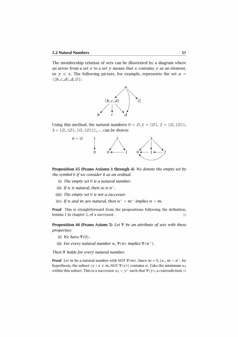
5.2 Natural Numbers 51
The membership relation of sets can be illustrated by a diagram where
an arrow from a set x to a set y means that x contains y as an element,
or y ∈ x. The following picture, for example, represents the set a ={{b, c, d}, d,∅}:
a
{b, c, d}
b c d
∅
Using this method, the natural numbers 0 = ∅,1 = {∅}, 2 = {∅, {∅}},3 = {∅, {∅}, {∅, {∅}}}, . . . can be drawn:
0 = ∅ 1
0
2
0 1
3
0 1 2
Proposition 45 (Peano Axioms 1 through 4) We denote the empty set by
the symbol 0 if we consider it as an ordinal.
(i) The empty set 0 is a natural number.
(ii) If n is natural, then so is n+.
(iii) The empty set 0 is not a successor.
(iv) If n and m are natural, then n+ =m+ implies n =m.
Proof This is straightforward from the propositions following the definition,
lemma 1 in chapter 2, of a successor. �
Proposition 46 (Peano Axiom 5) Let Ψ be an attribute of sets with these
properties:
(i) We have Ψ(0).
(ii) For every natural number n, Ψ(n) implies Ψ(n+).
Then Ψ holds for every natural number.
Proof Let m be a natural number with NOT Ψ(m). Since m ≠ 0, i.e., m = n+, by
hypothesis, the subset {x | x ∈m,NOT Ψ(x)} contains n. Take the minimum x0
within this subset. This is a successor x0 = y+ such that Ψ(y), a contradiction. �
52 Ordinal and Natural Numbers
Remark 7 Proposition 46 yields a proof scheme called “proof by induc-
tion”. One is given an attribute Ψ of sets, usually only specified for nat-
ural numbers. For other sets, we tacitly set Ψ to be false, but that value
is irrelevant for the given objective, which is to prove that Ψ holds for all
natural numbers. To this end, one proves (i) and (ii) in proposition 46 and
concludes as required.
The following proposition is the first result which follows from proposi-
tion 46, Peano’s fifth axiom:
Proposition 47 Let n be natural, and let a ⊊ n. Then there ism ∈ n such
that a∼→m.
Proof We prove the proposition by induction: For any natural number n, let
Ψ(n) be the proposition that for every proper subset y ⊂ n, there is a naturalm,
which is equipollent to y . Clearly, Ψ(0). Suppose that n =m+ and Ψ(m) holds.
Let y be a proper subset of n. If y ⊂m, either y =m and we are done, or y is a
proper subset ofm and the induction hypothesis gives us the required bijection.
Else, ifm ∈ y , there is an element u ∈m−y . But then y ′ = (y −{m})∪ {u} is
equipollent to y , and we are redirected to the above case. �
Proposition 48 Let n be a natural number, and suppose that an ordinal
a is equipollent to n. Then a = n. In particular, two natural numbers m
and n are equipollent iff they are equal.
Proof We prove the claim by induction and consider the property Ψ(n) for nat-
ural numbers defined by Ψ(n) iff for any ordinal a, the fact that a is equipollent
to n implies a = n. Suppose that there is a counterexample m; evidently m ≠ 0.
Let a ≠ m be ordinal, but equipollent to m. Let m = {x | x ∈ m,Ψ(x)}, which
is not empty, since it contains 0.
1. m = m. Since a and m are ordinal, either a ∈ m or m ∈ a. In the first
case, Ψ(a), which contradicts the choice of m. So m ∈ a and m ⊂ a is a proper
subset. Let f : a → m be a bijection. Then f(m) is a proper subset of m. By
proposition 47, there is an element n ∈ m which is equipollent to f(m) and
therefore also to m. But we know that Ψ(n), whence m = n, which contradicts
n ∈m.
2. m −m ≠ ∅. Take the smallest x0 in this difference set. There is an ordinal
b ≠ x0, but equipollent to x0. Then either b ∈ x0 or x0 ∈ b. In the first case,
b is a natural number in m since x0 ⊂ m. So b = x0 by construction of x0, a
contradiction. If x0 ∈ b, then since b is ordinal, x0 ⊂ b is a proper subset, and
we may proceed as in the first case above. This concludes the proof. �
5.2 Natural Numbers 53
Remark 8 This means that natural numbers describe in a unique way
certain cardinalities of ordinals. Each natural number represents exactly
one cardinality, and two different natural numbers are never equipollent.
Definition 26 A set a is called finite if it is equipollent to a natural num-
ber. This number is then called cardinality of a and denoted by card(a),
by #(a), or by |a|, depending on the usage.
This definition is justified by the fact that the cardinality of a finite set
is a unique number which is equipollent to that set, i.e., which in our
previous terminology has the same cardinality as the given set.
Corollary 49 A subset of a finite set is finite.
Proof We may suppose that we are dealing with a subset of a natural number,
where the claim is clear. �
Corollary 50 An ordinal set is finite iff it is a natural number.
Proof This follows right from proposition 48. �
Corollary 51 If an ordinal a is not finite, it contains all natural numbers.
Proof For any natural number n, we have either a ∈ n or a = n or n ∈ a. The
middle case is excluded by definition of a. The left alternative is excluded since
every subset of a finite set is finite. So every n is an element of a. �
Corollary 52 A finite set is not equipollent to a proper subset.
Proof In fact, a proper subset of a natural number n is equipollent to an element
of n, hence equal to this element, a contradiction. �
From the axiom 7 of infinity, we derive this result:
Proposition 53 There is an ordinal N whose elements are precisely the
natural numbers.
Proof This follows immediately from the axiom 7. �
Notation 5 The relation n ∈m for elements of N defines a well-ordering
among natural numbers. We denote it by n < m and say “n is smaller
than m” or else “m is larger than n”.
54 Ordinal and Natural Numbers
Exercise 19 With the well-ordering ≤ among natural numbers defined by
<, show that we have the following facts: Every non-empty set of natural
numbers has a (uniquely determined) minimal element. Let b be a limited
non-empty set of natural numbers, i.e., there is x ∈ N such that y < x for
all y ∈ b. Then there is a (uniquely determined) maximal element z ∈ b,
i.e., y ≤ z for all y ∈ b. Hint: Proceed by induction on b.

CHAPTER 6
Recursion Theorem
and Universal Properties
Before developing the arithmetic of natural numbers more specifically,
we describe some crucial methods for the construction of sets and func-
tions on sets. These properties are the basis of a fundamental branch in
mathematics, called topos theory, a branch which is of great importance
to computer science too, since it provides a marriage of formal logic and
geometry (see [36]).
Proposition 54 If a and b are two sets, then there is a set, denoted by
Set(a, b), whose elements are exactly the functions f : a→ b.
Proof The elements of the required set Set(a, b) are triples (a, f , b), where
f ⊂ a × b is a functional graph. So (a, f , b) = ((a, f ), b) ∈ (2a × 2a×b) × 2b,
whence Set(a, b) ⊂ (2a × 2a×b) × 2b is a subset selected by a straightforward
propositional attribute. �
Notation 6 The set Set(a, b) of functions is also denoted by ba if we want
to stress that it is a set, without emphasis on the specific nature, i.e., that
its elements are the functions f : a → b. This distinction may seem super-
fluous now, but we will understand this point when we will deal with more
general systems of objects and “functions” between such objects.
Example 17 Setting a = 0 (= ∅), we have Set(0, b) = {! :∅→ b}. Setting
b = 1 (= {0}), we have Set(a,1) = {! : a→ 1}. If a ≠ 0, then Set(a,0) = ∅.
56 Recursion Theorem and Universal Properties
6.1 Recursion Theorem
The set of functions allows a very important application of the fifth Peano
axiom (which is a theorem following from our set of axioms), namely
construction by induction. To this end, we need to look at functions f :
N→ a for any non-empty set a. If n ∈ N, we have the restriction f |n : n→a as declared in definition 13. Observe that f |n is defined for all natural
numbers strictly smaller than n, but not for n. If g : n+ → a is a function,
then we denote by g∗ the function g∗ : N → a with g∗(m) = g(n) for
m > n and g∗(m) = g(m) form ≤ n. If g is ! : 0→ a, we pick an element
g0 ∈ a and set g∗(m) = g0 for all natural numbersm. Here is the general
recursion theorem:
Proposition 55 (Recursion Theorem) Let a be a set, and let Φ : aN → aNbe a function such that for every natural number n, if f , g ∈ aN are such
that f |n = g|n, then Φ(f )(n) = Φ(g)(n). Then Φ has a unique fixpoint
LΦ ∈ aN, which means that Φ(LΦ) = LΦ. Consider the function Φn : an → awhich evaluates to Φn(g) = Φ(g∗)(n). Then we have
LΦ(0) = Φ0(! : 0→ a)LΦ(n
+) = Φn+(LΦ|n+).
Proof There is at most one such fixpoint. In fact, let L and M be two such
fixpoints, Φ(L) = L and Φ(M) = M , and suppose that they are different. Then
there is a smallest value n0 such that L(n0) ≠ M(n0). This means that L|n0 =M|n0 . But then Φ(L)(n0) = Φ(M)(n0), a contradiction. So there is at most one
such fixpoint. For every n ∈ N, let S(n) ⊂ an be the set of those functions
f : n → a such that for all m ∈ n, f(m) = Φm(f |m). Clearly, either S(n) is
empty or S(n) contains precisely one function gn. The set S(0) is not empty. Let
N+ be the smallest natural number such that S(N+) is empty. We may define a
function h : N+ → a by h|N = gN and h(N) = ΦN(h|N). But this is a function
in S(N+), so every S(n) is non-empty. Now define L(n) = gn+(n). Clearly, this
function is our candidate for a fixpoint: To begin with, if n < m, then evidently,
by the uniqueness of the elements of S(n), g(m)|n = g(n). Therefore, L|n = gnfor all n. And L is a fixpoint, in fact: L(n) = gn+(n) = Φn(gn+ |n) = Φn(gn) =Φ(g∗n)(n) = Φ(L)(n) since L|n = gn = g∗n |n. The claimed formula then follows
by construction. �
Remark 9 Very often, the above formal context will be treated in a rather
sloppy way. The common wording is this: One wants to define objects
(functions, sets of whatever nature) by the following data: one knows
6.1 Recursion Theorem 57
which object O0 you have to start with, i.e., the natural number 0. Then
you suppose that you have already “constructed” the objects Om, m ≤ nfor a natural number n, and your construction of On+ for the successor
n+ is given from O0, O1, . . .On and some “formula” Φ. Then you have
defined the objects On for every n ∈ N.
Example 18 In order to clarify the rather abstract recursion theorem, we
shall apply it to the definition of the function c+? : N → N which will be
discussed in depth in the next chapter. Intuitively, we want this function
to behave as follows:c + 0 = c
c + b+ = (c + b)+
This corresponds to a function Φ : NN → NN given by Φ(f )(0) = c, and
Φ(f )(n+) = (f (n))+. This Φ satisfies the condition for the recursion
theorem: Let f , g ∈ NN be two functions with f |n+ = g|n+ . In particu-
lar, this implies that f(n) = g(n). Then, Φ(f )(0) = c = Φ(g)(0), and
Φ(f )(n+) = (f (n))+ = (g(n))+ = Φ(g)(n+). The recursion theorem now
states that Φ has a fixpoint LΦ ∈ NN with the property that
LΦ(0) = Φ0(! : 0→ N) = Φ((! : 0→ N)∗)(0) = c,
and
LΦ(n+) = Φn+(LΦ|n+)= Φ((LΦ|n+)∗)(n+)= ((LΦ|n+)∗(n))+= (LΦ|n+(n))+= LΦ(n)+.
This is exactly the behavior we requested for our function c+?.
Exercise 20 Assuming the availability of the multiplication of natural
numbers (which will be introduced in the next chapter), let the factorial
function fact : N→ N be given by
fact(0) = 1 and fact(n+) = n+ · fact(n).
Explicitly write down the function Φ corresponding to this recursive def-
inition of fact, show that Φ satisfies the condition for the application of
the recursion theorem, and show that the function LΦ is equal to the
function fact.
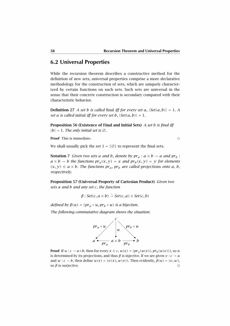
58 Recursion Theorem and Universal Properties
6.2 Universal Properties
While the recursion theorem describes a constructive method for the
definition of new sets, universal properties comprise a more declarative
methodology for the construction of sets, which are uniquely character-
ized by certain functions on such sets. Such sets are universal in the
sense that their concrete construction is secondary compared with their
characteristic behavior.
Definition 27 A set b is called final iff for every set a, |Set(a, b)| = 1. A
set a is called initial iff for every set b, |Set(a, b)| = 1.
Proposition 56 (Existence of Final and Initial Sets) A set b is final iff
|b| = 1. The only initial set is ∅.
Proof This is immediate. �
We shall usually pick the set 1 = {∅} to represent the final sets.
Notation 7 Given two sets a and b, denote by pra : a × b → a and prb :
a × b → b the functions pra(x,y) = x and prb(x,y) = y for elements
(x,y) ∈ a × b. The functions pra, prb are called projections onto a, b,
respectively.
Proposition 57 (Universal Property of Cartesian Product) Given two
sets a and b and any set c, the function
β : Set(c, a× b) ∼→ Set(c, a)× Set(c, b)
defined by β(u) = (pra ◦u,prb ◦u) is a bijection.
The following commutative diagram shows the situation:
c
a ðpra
pra ◦u
ða× b
u
�
prbñ b
prb ◦u
ñ
Proof If u : c → a×b, then for every x ∈ c, u(x) = (pra(u(x)),prb(u(x))), so u
is determined by its projections, and thus β is injective. If we are given v : c → aand w : c → b, then define u(x) = (v(x),w(x)). Then evidently, β(u) = (v,w),so β is surjective. �
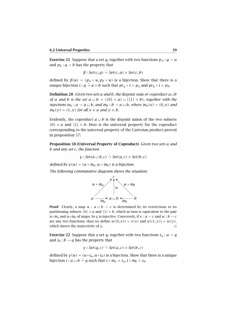
6.2 Universal Properties 59
Exercise 21 Suppose that a set q, together with two functions pa : q → aand pb : q → b has the property that
β : Set(c, q)∼→ Set(c, a)× Set(c, b)
defined by β(u) = (pa ◦ u,pb ◦ u) is a bijection. Show that there is a
unique bijection i : q∼→ a× b such that pra ◦ i = pa and prb ◦ i = pb.
Definition 28 Given two sets a and b, the disjoint sum or coproduct atbof a and b is the set a t b = ({0} × a) ∪ ({1} × b), together with the
injections ina : a → at b, and inb : b → at b, where ina(x) = (0, x) and
inb(y) = (1, y) for all x ∈ a and y ∈ b.
Evidently, the coproduct a t b is the disjoint union of the two subsets
{0} × a and {1} × b. Here is the universal property for the coproduct
corresponding to the universal property of the Cartesian product proved
in proposition 57:
Proposition 58 (Universal Property of Coproduct) Given two sets a and
b and any set c, the function
γ : Set(at b, c) ∼→ Set(a, c)× Set(b, c)
defined by γ(u) = (u ◦ ina, u ◦ inb) is a bijection.
The following commutative diagram shows the situation:
c
aina
ñ
u ◦ ina
ñ
at b
u
�
ðinb
b
u ◦ inb
ð
Proof Clearly, a map u : a t b → c is determined by its restrictions to its
partitioning subsets {0} × a and {1} × b, which in turn is equivalent to the pair
u◦ina and u◦inb of maps. So γ is injective. Conversely, if v : a→ c andw : b → care any two functions, then we define u((0, x)) = v(x) and u((1, y)) = w(y),which shows the surjectivity of γ. �
Exercise 22 Suppose that a set q, together with two functions ia : a → qand ib : b → q has the property that
γ : Set(q, c)∼→ Set(a, c)× Set(b, c)
defined by γ(u) = (u◦ia, u◦ib) is a bijection. Show that there is a unique
bijection i : at b ∼→ q such that i ◦ ina = ia, i ◦ inb = ib.
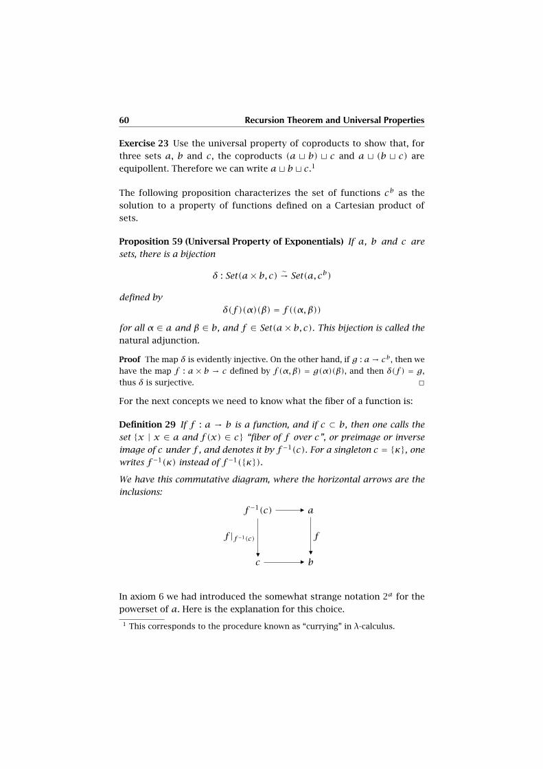
60 Recursion Theorem and Universal Properties
Exercise 23 Use the universal property of coproducts to show that, for
three sets a, b and c, the coproducts (a t b) t c and a t (b t c) are
equipollent. Therefore we can write at b t c.1
The following proposition characterizes the set of functions cb as the
solution to a property of functions defined on a Cartesian product of
sets.
Proposition 59 (Universal Property of Exponentials) If a, b and c are
sets, there is a bijection
δ : Set(a× b, c) ∼→ Set(a, cb)
defined by
δ(f)(α)(β) = f((α,β))for all α ∈ a and β ∈ b, and f ∈ Set(a× b, c). This bijection is called the
natural adjunction.
Proof The map δ is evidently injective. On the other hand, if g : a→ cb, then we
have the map f : a × b → c defined by f(α,β) = g(α)(β), and then δ(f) = g,
thus δ is surjective. �
For the next concepts we need to know what the fiber of a function is:
Definition 29 If f : a → b is a function, and if c ⊂ b, then one calls the
set {x | x ∈ a and f(x) ∈ c} “fiber of f over c”, or preimage or inverse
image of c under f , and denotes it by f−1(c). For a singleton c = {κ}, one
writes f−1(κ) instead of f−1({κ}).We have this commutative diagram, where the horizontal arrows are the
inclusions:
f−1(c) ñ a
c
f |f−1(c)
�ñ b
f
�
In axiom 6 we had introduced the somewhat strange notation 2a for the
powerset of a. Here is the explanation for this choice.
1 This corresponds to the procedure known as “currying” in λ-calculus.
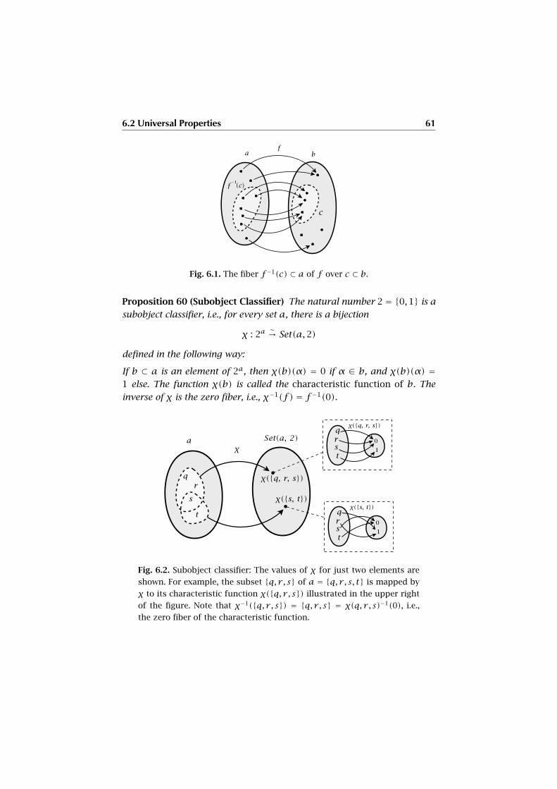
6.2 Universal Properties 61
Fig. 6.1. The fiber f−1(c) ⊂ a of f over c ⊂ b.
Proposition 60 (Subobject Classifier) The natural number 2 = {0,1} is a
subobject classifier, i.e., for every set a, there is a bijection
χ : 2a∼→ Set(a,2)
defined in the following way:
If b ⊂ a is an element of 2a, then χ(b)(α) = 0 if α ∈ b, and χ(b)(α) =1 else. The function χ(b) is called the characteristic function of b. The
inverse of χ is the zero fiber, i.e., χ−1(f ) = f−1(0).
Fig. 6.2. Subobject classifier: The values of χ for just two elements are
shown. For example, the subset {q, r , s} of a = {q, r , s, t} is mapped by
χ to its characteristic function χ({q, r , s}) illustrated in the upper right
of the figure. Note that χ−1({q, r , s}) = {q, r , s} = χ(q, r , s)−1(0), i.e.,
the zero fiber of the characteristic function.
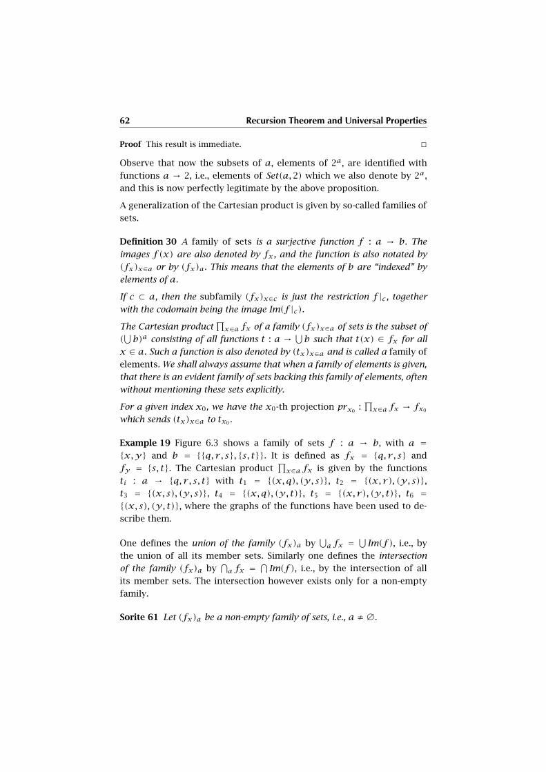
62 Recursion Theorem and Universal Properties
Proof This result is immediate. �
Observe that now the subsets of a, elements of 2a, are identified with
functions a → 2, i.e., elements of Set(a,2) which we also denote by 2a,
and this is now perfectly legitimate by the above proposition.
A generalization of the Cartesian product is given by so-called families of
sets.
Definition 30 A family of sets is a surjective function f : a → b. The
images f(x) are also denoted by fx , and the function is also notated by
(fx)x∈a or by (fx)a. This means that the elements of b are “indexed” by
elements of a.
If c ⊂ a, then the subfamily (fx)x∈c is just the restriction f |c , together
with the codomain being the image Im(f |c).The Cartesian product
∏x∈a fx of a family (fx)x∈a of sets is the subset of
(⋃b)a consisting of all functions t : a → ⋃
b such that t(x) ∈ fx for all
x ∈ a. Such a function is also denoted by (tx)x∈a and is called a family of
elements. We shall always assume that when a family of elements is given,
that there is an evident family of sets backing this family of elements, often
without mentioning these sets explicitly.
For a given index x0, we have the x0-th projection prx0:∏x∈a fx → fx0
which sends (tx)x∈a to tx0 .
Example 19 Figure 6.3 shows a family of sets f : a → b, with a ={x,y} and b = {{q, r , s}, {s, t}}. It is defined as fx = {q, r , s} and
fy = {s, t}. The Cartesian product∏x∈a fx is given by the functions
ti : a → {q, r , s, t} with t1 = {(x, q), (y, s)}, t2 = {(x, r), (y, s)},t3 = {(x, s), (y, s)}, t4 = {(x, q), (y, t)}, t5 = {(x, r), (y, t)}, t6 ={(x, s), (y, t)}, where the graphs of the functions have been used to de-
scribe them.
One defines the union of the family (fx)a by⋃a fx =
⋃Im(f ), i.e., by
the union of all its member sets. Similarly one defines the intersection
of the family (fx)a by⋂a fx =
⋂Im(f ), i.e., by the intersection of all
its member sets. The intersection however exists only for a non-empty
family.
Sorite 61 Let (fx)a be a non-empty family of sets, i.e., a ≠∅.
6.2 Universal Properties 63
Fig. 6.3. A family of sets f : a→ b.
(i) The Cartesian product∏x∈a fx is non-empty iff each fx is non-
empty.
(ii) If all sets fx coincide and are equal to c, then∏x∈a fx = ca.
(iii) If a = 2, then∏x∈2 fx
∼→ f0 × f1.
(iv) If (ux : d → fx)x∈a is a family of functions, then there is a unique
function u : d→∏x∈a fx such that ux = prx ◦u for all x ∈ a.
Proof (i) By definition, the Cartesian product is non-empty for a ≠∅ iff each fxis so.
(ii) This is an immediate consequence of the definition of the Cartesian product
and of the fact that here, c = ⋃x∈a c.(iii) The functions g : 2→ f0∪f1, where g(0) ∈ f0 and g(1) ∈ f1, are in bijection
with the pairs of their evaluations (g(0), g(1)) ∈ f0 × f1.
(iv) The reader should think about the set where the family of functions is de-
duced. But if this is done, the statement is immediate. �
Example 20 Families where the index set a is a natural number n or
the set N of all natural numbers are called sequences. For a = n, we
have the finite sequences (ti)i∈n, or, in an equivalent notation, (ti)i<n.
One then often writes ti, i = 0,1, . . . n − 1 instead, or also t0, t1, . . . tn−1.
For a = N, one writes also (ti)i=0,1,2,... or else t0, t1, . . .. The length of a
sequence (ti)i∈n is the (uniquely determined) number n. One also calls
such a sequence an n-tuple.
In computer science, one often calls sequences lists, and it is also agreed
that list indexes start with 0, as do natural number indexes. The empty
list is also that sequence with index set a = 0, the empty set.
64 Recursion Theorem and Universal Properties
Exercise 24 Prove that there is exactly one empty family, i.e., a family
with an empty index set.
Cartesian products∏x∈a fx also admit linear orderings if their members
do so. Here is the precise definition of the so-called “lexicographic order-
ing”:
Definition 31 Suppose that we are given a family (fx)a of sets such that
each fx bears a linear ordering <x , and such that the index set a is well-
ordered by the relation <. Then, for two different families (tx)a, (sx)a ∈∏x∈a fx the relation
(tx)a ≺ (sx)a iff the smallest index y , where ty ≠ sy , has ty <y sy
is called the lexicographic ordering on∏x∈a fx .
Lemma 62 The lexicographic ordering is a linear ordering.
Proof According to lemma 26, we show that ≺ is transitive, antisymmetric and
total. Let (tx)a ≺ (sx)a ≺ (ux)a. If the smallest index y , where these three
families differ, is the same, then transitivity follows from transitivity of the total
ordering at this index. Else, one of the two smallest indexes is smaller than the
other, let y1 < y2 for the index y1 of the left pair (tx)a ≺ (sx)a. Then the
inequalities at this index are ty1 <y1 sy1 = uy1 , whence ty1 <y1 uy1 , i.e., (tx)a ≺(ux)a; similarly for the other situation, namely, y2 < y1. The same argument
works for antisymmetry. As to totality: Let (tx)a and (sx)a be any two families. If
they are different, then the smallest index y where they differ has either ty <y syor sy <y ty since <y is total. �
Exercise 25 Show that the lexicographic ordering on∏n∈N fn is a well-
ordering iff each linear ordering <n on fn is so. The same is true for a
finite sequence of sets, i.e., for∏n<N fn, where N ∈ N.
Exercise 26 Suppose that we are given a finite alphabet set A of “let-
ters”. Suppose that a bijection u : A ∼→ N with the natural number
N = card(A) is fixed, and consider the ordering of letters induced by
this bijection, i.e., X < Y iff u(X) < u(Y). Suppose that an element ∈Ais selected. Consider now the restriction of the lexicographic ordering on
AN to the subsetA(N) consisting of all sequences (τn)N such that τn =for all but a finite number of indexes. Show that this set may be identi-
fied with the set of all finite words in the given alphabet. Show that the
6.2 Universal Properties 65
induced lexicographic ordering on A(N) coincides with the usual lexico-
graphic ordering in a dictionary of words from the alphabet A; here the
special sign plays the role of the empty space unit.
The name “lexicographic” effectively originates in the use of such an or-
dering in compiling dictionaries. As an example we may consider words
of length 4, i.e., the setA4. Let the ordering onA be < A < B . . .Z. Then,
writing the sequence (ti)i=0,1,2,3, ti ∈A as t0t1t2t3, we have, for instance:
BALD ≺ BAR ≺ BASH ≺ I AM ≺ MAN ≺ MANE ≺ MAT ≺ SO ≺ SORE
The minimal element ofA4 is , the maximal element is ZZZZ.
Definition 32 If (fx)a is a family of sets, where each set fx bears a binary
relation Rx , then the Cartesian product∏x∈a fx bears the product relation
R =∏x∈a Rx which is defined “coordinatewise”, i.e.,
(tx)aR(sx)a iff tx Rx sx for each x ∈ a.
Attention: Even if each binary relation on the set fx is a linear ordering.
Therefore product relation is not, in general, a linear ordering, so the
lexicographic ordering is a remarkable construction since it “preserves”
linear orderings.
Until now, we only considered binary relations. By use of Cartesian prod-
ucts of families of sets, one can now introduce the concept of an n-ary
relation for n ∈ N as follows:
Definition 33 If n is a natural number and a is a set, an n-ary relation
on a is a subset R of the n-fold Cartesian product an, the binary relation
being the special case of n = 2.
Not every binary relation is an equivalence relation, but very often, one
is interested in a kind of minimal equivalence relation which contains a
given relation. Here is the precise setup:
Lemma 63 If (Rx)a is a non-empty family of equivalence relations on a set
b, then the intersection⋂a Rx is an equivalence relation. It is the largest
equivalence relation (for the subset inclusion relation), which is contained
in all relations Rx, x ∈ a.
Proof This is straightforward to check. �
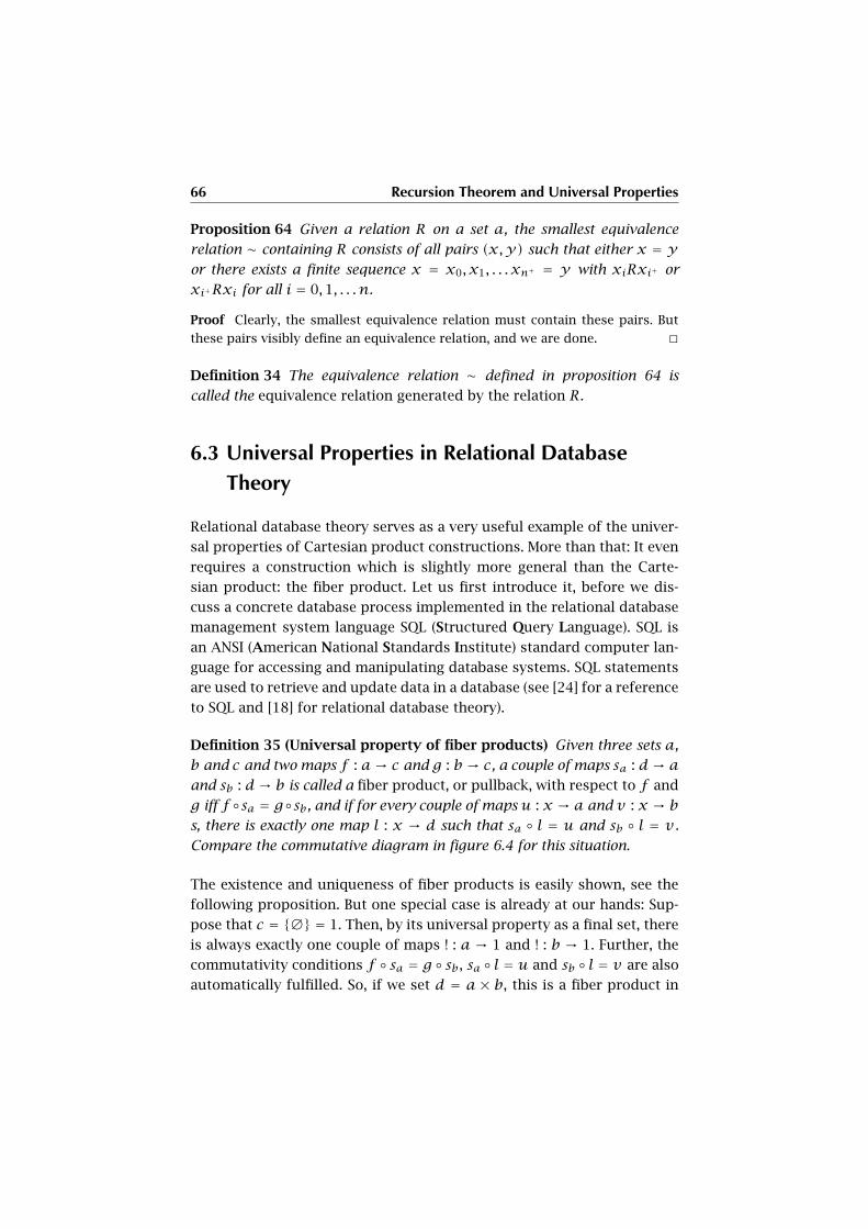
66 Recursion Theorem and Universal Properties
Proposition 64 Given a relation R on a set a, the smallest equivalence
relation ∼ containing R consists of all pairs (x,y) such that either x = yor there exists a finite sequence x = x0, x1, . . . xn+ = y with xiRxi+ or
xi+Rxi for all i = 0,1, . . . n.
Proof Clearly, the smallest equivalence relation must contain these pairs. But
these pairs visibly define an equivalence relation, and we are done. �
Definition 34 The equivalence relation ∼ defined in proposition 64 is
called the equivalence relation generated by the relation R.
6.3 Universal Properties in Relational Database
Theory
Relational database theory serves as a very useful example of the univer-
sal properties of Cartesian product constructions. More than that: It even
requires a construction which is slightly more general than the Carte-
sian product: the fiber product. Let us first introduce it, before we dis-
cuss a concrete database process implemented in the relational database
management system language SQL (Structured Query Language). SQL is
an ANSI (American National Standards Institute) standard computer lan-
guage for accessing and manipulating database systems. SQL statements
are used to retrieve and update data in a database (see [24] for a reference
to SQL and [18] for relational database theory).
Definition 35 (Universal property of fiber products) Given three sets a,
b and c and two maps f : a→ c and g : b → c, a couple of maps sa : d→ aand sb : d→ b is called a fiber product, or pullback, with respect to f and
g iff f ◦sa = g◦sb, and if for every couple of maps u : x → a and v : x → bs, there is exactly one map l : x → d such that sa ◦ l = u and sb ◦ l = v .
Compare the commutative diagram in figure 6.4 for this situation.
The existence and uniqueness of fiber products is easily shown, see the
following proposition. But one special case is already at our hands: Sup-
pose that c = {∅} = 1. Then, by its universal property as a final set, there
is always exactly one couple of maps ! : a → 1 and ! : b → 1. Further, the
commutativity conditions f ◦ sa = g ◦ sb, sa ◦ l = u and sb ◦ l = v are also
automatically fulfilled. So, if we set d = a × b, this is a fiber product in
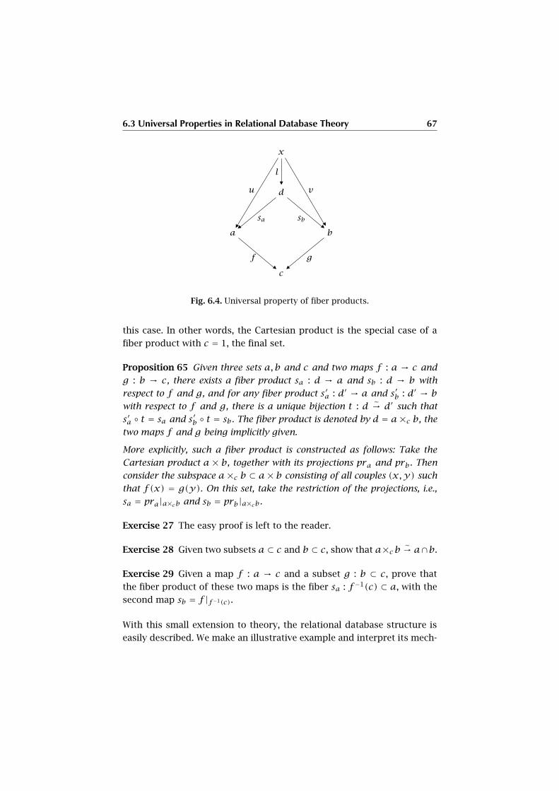
6.3 Universal Properties in Relational Database Theory 67
x
d
l�
a
u
ð
sað
b
v
ñ
sbñ
c
g
ð
fñ
Fig. 6.4. Universal property of fiber products.
this case. In other words, the Cartesian product is the special case of a
fiber product with c = 1, the final set.
Proposition 65 Given three sets a,b and c and two maps f : a → c and
g : b → c, there exists a fiber product sa : d → a and sb : d → b with
respect to f and g, and for any fiber product s′a : d′ → a and s′b : d′ → bwith respect to f and g, there is a unique bijection t : d
∼→ d′ such that
s′a ◦ t = sa and s′b ◦ t = sb. The fiber product is denoted by d = a×c b, the
two maps f and g being implicitly given.
More explicitly, such a fiber product is constructed as follows: Take the
Cartesian product a × b, together with its projections pra and prb. Then
consider the subspace a×c b ⊂ a× b consisting of all couples (x,y) such
that f(x) = g(y). On this set, take the restriction of the projections, i.e.,
sa = pra|a×cb and sb = prb|a×cb.
Exercise 27 The easy proof is left to the reader.
Exercise 28 Given two subsets a ⊂ c and b ⊂ c, show that a×cb ∼→ a∩b.
Exercise 29 Given a map f : a → c and a subset g : b ⊂ c, prove that
the fiber product of these two maps is the fiber sa : f−1(c) ⊂ a, with the
second map sb = f |f−1(c).
With this small extension to theory, the relational database structure is
easily described. We make an illustrative example and interpret its mech-

68 Recursion Theorem and Universal Properties
anisms in terms of the fiber product and other set-theoretical construc-
tions.
To begin with, one is given domains from where values can be taken.
However, these domains also have a name, not only values. We therefore
consider sets with specific names X, but also isomorphisms X∼→ VX with
given sets of values. Then, whenever we need to take elements x ∈ X,
their values will be taken to lie in VX , so that we may distinguish the
elements, but nevertheless compare their values. In our example, we con-
sider these sets of values: INTEGER = {1,2,3,4,5 . . .}, this is a finite set
of numbers (we assume that these are given, we shall discuss the precise
definition of numbers later), whose size is defined by the standard imple-
mentation of numbers on a given operating system. Next, we are given a
set
TEXT = {Apples,Cookies,Oranges,Donald Duck,
Mickey Mouse,Goofy,Bunny, Shrek, . . .}of words, which also depends on the computer memory (again, words in
a formal sense will be defined later). We now need the sets:
ORDER_ID∼→ INTEGER
CUSTOMER_ID∼→ INTEGER
PRODUCT∼→ TEXT
NAME∼→ TEXT
ADDRESS∼→ TEXT
We consider two subsets ORDERS and CUSTOMERS, called relations in
database theory,
ORDERS ⊂ ORDER_ID× PRODUCT× CUSTOMER_ID
CUSTOMERS ⊂ CUSTOMER_ID×NAME×ADDRESS
which we specify as follows, to be concrete. The set ORDERS:
ORDER_ID PRODUCT CUSTOMER_ID
7 Apples 3
8 Apples 4
11 Oranges 3
13 Cookies 3
77 Oranges 7
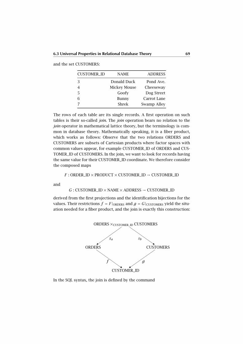
6.3 Universal Properties in Relational Database Theory 69
and the set CUSTOMERS:
CUSTOMER_ID NAME ADDRESS
3 Donald Duck Pond Ave.
4 Mickey Mouse Cheeseway
5 Goofy Dog Street
6 Bunny Carrot Lane
7 Shrek Swamp Alley
The rows of each table are its single records. A first operation on such
tables is their so-called join. The join operation bears no relation to the
join operator in mathematical lattice theory, but the terminology is com-
mon in database theory. Mathematically speaking, it is a fiber product,
which works as follows: Observe that the two relations ORDERS and
CUSTOMERS are subsets of Cartesian products where factor spaces with
common values appear, for example CUSTOMER_ID of ORDERS and CUS-
TOMER_ID of CUSTOMERS. In the join, we want to look for records having
the same value for their CUSTOMER_ID coordinate. We therefore consider
the composed maps
F : ORDER_ID× PRODUCT× CUSTOMER_ID→ CUSTOMER_ID
and
G : CUSTOMER_ID×NAME×ADDRESS→ CUSTOMER_ID
derived from the first projections and the identification bijections for the
values. Their restrictions f = F|ORDERS and g = G|CUSTOMERS yield the situ-
ation needed for a fiber product, and the join is exactly this construction:
ORDERS×CUSTOMER_ID CUSTOMERS
ORDERS
sa
ðCUSTOMERS
sbñ
CUSTOMER_ID
g
ð
f
ñ
In the SQL syntax, the join is defined by the command
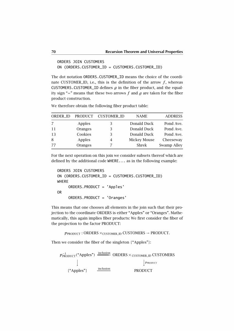
70 Recursion Theorem and Universal Properties
ORDERS JOIN CUSTOMERS
ON (ORDERS.CUSTOMER_ID = CUSTOMERS.CUSTOMER_ID)
The dot notation ORDERS.CUSTOMER_ID means the choice of the coordi-
nate CUSTOMER_ID, i.e., this is the definition of the arrow f , whereas
CUSTOMERS.CUSTOMER_ID defines g in the fiber product, and the equal-
ity sign “=” means that these two arrows f and g are taken for the fiber
product construction.
We therefore obtain the following fiber product table:
ORDER_ID PRODUCT CUSTOMER_ID NAME ADDRESS
7 Apples 3 Donald Duck Pond Ave.
11 Oranges 3 Donald Duck Pond Ave.
13 Cookies 3 Donald Duck Pond Ave.
8 Apples 4 Mickey Mouse Cheeseway
77 Oranges 7 Shrek Swamp Alley
For the next operation on this join we consider subsets thereof which are
defined by the additional code WHERE... as in the following example:
ORDERS JOIN CUSTOMERS
ON (ORDERS.CUSTOMER_ID = CUSTOMERS.CUSTOMER_ID)
WHERE
ORDERS.PRODUCT = ’Apples’
OR
ORDERS.PRODUCT = ’Oranges’
This means that one chooses all elements in the join such that their pro-
jection to the coordinate ORDERS is either “Apples” or “Oranges”. Mathe-
matically, this again implies fiber products: We first consider the fiber of
the projection to the factor PRODUCT:
pPRODUCT : ORDERS×CUSTOMER_ID CUSTOMERS→ PRODUCT.
Then we consider the fiber of the singleton {“Apples”}:
p−1PRODUCT(“Apples”)
inclusion-------------------------------------------------------------------------------------------------------------------------------------------------------------------→ ORDERS×CUSTOMER_ID CUSTOMERS
yypPRODUCT
{“Apples”} inclusion-------------------------------------------------------------------------------------------------------------------------------------------------------------------→ PRODUCT
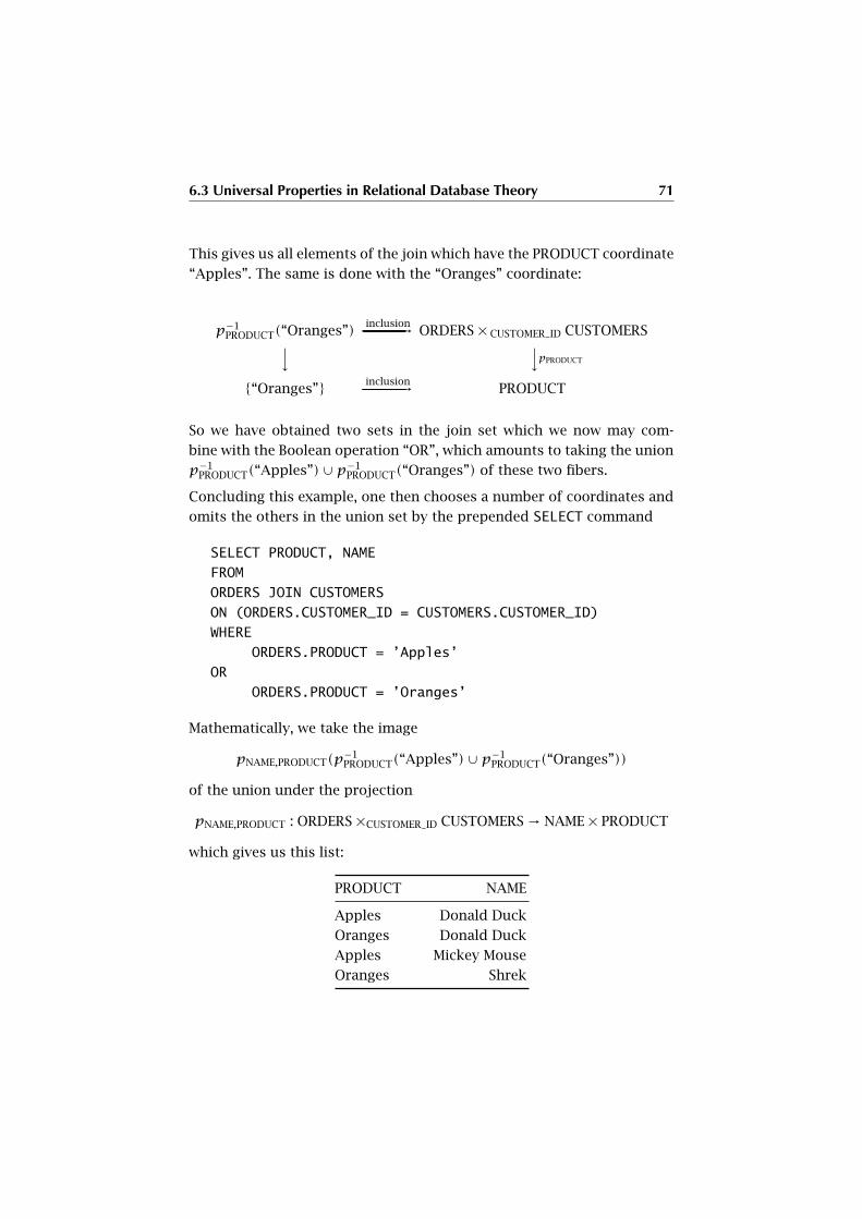
6.3 Universal Properties in Relational Database Theory 71
This gives us all elements of the join which have the PRODUCT coordinate
“Apples”. The same is done with the “Oranges” coordinate:
p−1PRODUCT(“Oranges”)
inclusion-------------------------------------------------------------------------------------------------------------------------------------------------------------------→ ORDERS×CUSTOMER_ID CUSTOMERS
yypPRODUCT
{“Oranges”} inclusion-------------------------------------------------------------------------------------------------------------------------------------------------------------------→ PRODUCT
So we have obtained two sets in the join set which we now may com-
bine with the Boolean operation “OR”, which amounts to taking the union
p−1PRODUCT(“Apples”)∪ p−1
PRODUCT(“Oranges”) of these two fibers.
Concluding this example, one then chooses a number of coordinates and
omits the others in the union set by the prepended SELECT command
SELECT PRODUCT, NAME
FROM
ORDERS JOIN CUSTOMERS
ON (ORDERS.CUSTOMER_ID = CUSTOMERS.CUSTOMER_ID)
WHERE
ORDERS.PRODUCT = ’Apples’
OR
ORDERS.PRODUCT = ’Oranges’
Mathematically, we take the image
pNAME,PRODUCT(p−1PRODUCT(“Apples”)∪ p−1
PRODUCT(“Oranges”))
of the union under the projection
pNAME,PRODUCT : ORDERS×CUSTOMER_ID CUSTOMERS→ NAME× PRODUCT
which gives us this list:
PRODUCT NAME
Apples Donald Duck
Oranges Donald Duck
Apples Mickey Mouse
Oranges Shrek
CHAPTER 7
Natural Arithmetic
This chapter is central insofar as the basic arithmetic operations, i.e.,
addition, multiplication, and exponentiation of natural numbers are in-
troduced, operations which are the seed of the entire mathematical cal-
culations.
7.1 Natural Operations
All these operations are defined by recursion, i.e., by applying the recur-
sion theorem 55.
Definition 36 Given a natural number a, addition to a is recursively de-
fined as the function1 a+ ? : N→ N which evaluates to
a+ 0 = a and a+ b+ = (a+ b)+.Supposing that addition is defined, multiplication with a is defined as the
function a · ? : N→ N which evaluates to
a · 0 = 0 and a · (b+) = (a · b)+ a.Supposing that addition and multiplication are defined, exponentiation of
a ≠ 0 is defined as the function a? : N→ N which evaluates to
a0 = 1 and a(b+) = (ab) · a.
If a = 0, we define 00 = 1 and 0b = 0 for b ≠ 0.
1 When defining function symbols, the question mark is used to indicate the
position of the arguments.
74 Natural Arithmetic
Evidently, a+ = a+1, and from now on we identify these two expressions.
The number a+b is called the sum of a and b. The number a ·b is called
the product of a and b. These operations share the following properties.
All these properties can be demonstrated by induction.
Sorite 66 Let a,b, c be natural numbers. We have these laws:
(i) (Additive neutral element) a+ 0 = 0+ a = a,
(ii) (Additive associativity) a+ (b+ c) = (a+ b)+ c, which is therefore
written as a+ b + c,(iii) (Additive commutativity) a+ b = b + a,
(iv) (Multiplicative neutral element) a · 1 = 1 · a = a,
(v) (Multiplicative associativity) a·(b·c) = (a·b)·c, which is therefore
written as a · b · c,(vi) (Multiplicative commutativity) a · b = b · a,
(vii) (Multiplication distributivity) a · (b + c) = a · b + a · c,(viii) (Exponential neutral element) a1 = a,
(ix) (Exponentiation (+)-distributivity) ab+c = ab · ac ,(x) (Exponentiation (·)-distributivity) (a · b)c = ac · bc ,
(xi) (Additive monotony) if a < b, then a+ c < b + c,(xii) (Multiplicative monotony) if c ≠ 0 and a < b, then a · c < b · c,
(xiii) (Exponential base monotony) if c ≠ 0 and a < b, then ac < bc ,
(xiv) (Exponential exponent monotony) if c ≠ 0,1 and a < b, then ca <
cb,
(xv) (Ordering of operations) if a,b > 1, then a+ b ≤ a · b ≤ ab.
Proof (i) We have a + 0 = a by definition, while 0 + (a+) = (0 + a)+ = a+ by
recursion on a.
(ii) This is true for c = 0 by (i). By recursion on c, we have a + (b + c+) =a+ ((b + c)+) = (a+ (b + c))+ = ((a+ b)+ c)+ = (a+ b)+ c+.
(iii) This is true for b = 0 by (i). We also have a + 1 = 1 + a, in fact, this is true
for a = 0, and by recursion, (a+)+ = (a + 1)+ = (a + (1+)) = a + (1 + 1) =(a+1)+1 = (a+)+1. By recursion on b, we have a+b+ = (a+b)+ = (b+a)+ =b + (a+) = b + (a+ 1) = b + (1+ a) = (b + 1)+ a = b+ + a.
(iv) We have a · 1 = (a · 0) + a = 0 + a = a. Therefore 1 · 0 = 0 = 0 · 1, while
1 · a+ = (1 · a)+ 1 = a+ 1 = a+.
(vii) We have a · (b + c) = a · b + a · c for c = 0. By recursion on c we have
a · (b + c+) = a · ((b + c)+) = a · (b + c)+ a = a · b + a · c + a = a · b + a · c+.
7.1 Natural Operations 75
(v) For c = 0,1 we have associativity by the previous results. By recursion on c we
have a·(b·c+) = a·(b·c+b) = a·(b·c)+a·b = (a·b)·c+(a·b)·1 = (a·b)·c+.
(vi) Commutativity is known for b = 1. By recursion on b we have a · b+ =a · (b + 1) = a · b + a = b · a+ a = 1 · a+ b · a = (1+ b) · a = b+ · a.
(viii) We have a1 = a0 · a = 1 · a = a.
(ix) We have a(b+0) = ab = ab·a0, and a(b+c+) = a((b+c)+) = a(b+c)·a = ab·ac·a =ab · (ac · a) = ab · a(c+).(x) We have (a · b)0 = 1 = 1 · 1 = a0 · b0, and (a · b)(c+) = (a · b)c · (a · b) =ac · bc · a · b = (ac · a) · (bc · b) = a(c+) · b(c+).(xi) If a < b, then a+ 0 < b+ 0, and a+ c+ = (a+ c)+ < (b+ c)+ = b+ c+, since
x < y implies x+ < y+ by lemma 41 (ii).
(xii) If a < b, then a·1 < b ·1, and a·c+ = a·c+a < b ·c+a < b ·c+b = b ·c+.
(xiii) For a = 0 or c = 1 it is clear, suppose a ≠ 0 and do recursion on c. Then
a(c+) = ac · a < bc · a < bc · b = b(c+).
(xiv) For b = a+ it is clear, so suppose b = d+, a < d. Then by recursion on b,
ca < cd and therefore cd < cd · c = cb.(xv) To begin with denote 1+ = 2 (attention: we still have not introduced the
common notation for natural numbers) and take b = 2. Then a+2 ≤ a·2 ≤ a2 is
easily proved by induction on a, starting with the famous equality 2+2 = 2 ·2 =22. We then prove the inequalities by induction on b, the details being left to be
completed by the reader. �
Proposition 67 If a and b are natural numbers such that a ≤ b, then
there is exactly one natural number c such that a+ c = b.
Proof We use induction on b. If b = a, then c = 0 solves the problem. If b > a,
then b = d+ with d ≥ a. Then, since d < b, we can use the induction hypothesis
to find e, such that a+e = d. We set c = e+, and we have by definition of addition
a + c = a + e+ = (a + e)+ = d+ = b. If c and c′ are two different solutions, we
must have c < c′, for example. Then monotony implies a+ c < a+ c′, i.e., b < b,
a contradiction. �
If n is a natural number different from 0, we may look for the unique m,
such that m + 1 = n. Clearly, it is the m such that n = m+. This is the
predecessor of n, which we denote by n−1, a notation which will become
clear later, when subtraction has been defined.

76 Natural Arithmetic
7.2 Euclid and the Normal Forms
The following theorem is Euclid’s so-called “division theorem”. It is a cen-
tral tool for the common representation of natural, and also rational and
real numbers in the well-known decimal format. Moreover, it is the cen-
tral step in the calculation of the greatest common divisor of two natural
numbers by the Euclidean algorithm2, see chapter 16.
Proposition 68 (Division Theorem) If a and b are natural numbers with
b ≠ 0, then there is a unique pair q and r of natural numbers with r < b
such that
a = q · b + r .Proof Existence: Let t be the minimal natural number such that a < t · b. For
example, according to sorite 66, a < a · b, so t exists and evidently is non-
zero, t = q+. This means that q ·b ≤ a. So by proposition 67, there is r such that
a = q·b+r . If b ≤ r we have r = b+p, and by the choice of t, a = q·b+b+p =(q + 1)b + p = t · b + p > a, a contradiction. So the existence is proved.
Uniqueness: If we have two representations a = q·b+r = q′ ·b+r ′ with q′ ≥ q+,
then we have a = q′ · b + r ′ ≥ r · b + b + r ′ > q · b + r = a, a contradiction. So
q = q′, and equality of r and r ′ follows from proposition 67. �
Proposition 69 If a and b are natural numbers with a ≠ 0 and b ≠ 0,1,
then there is a unique triple c, s, r of natural numbers with r < bc and
0 < s < b such that
a = s · bc + r .Proof Let t be the minimal natural number such that a < bt , and clearly t =w+1. Such a t exists since a < b+a ≤ b ·a ≤ ba by sorite 66. Therefore a ≥ bw .
We now apply proposition 68 and have a = r · bw + s, s < bw . Now, if r = b+p,
then we also have a = (b + p) · bw + s = bt + p · bw + s, a contradiction to the
choice of t. So we have one such desired representation. Uniqueness follows by
the usual contradiction from different s coefficients, and then form different r ’s
for equal s coefficients. �
In order to define the b-adic representation of a natural number, of which
the decimal (10-adic) representation is a special case, we need to define
2 An algorithm is a detailed sequence of actions (steps), starting from a given
input, to perform in order to accomplish some task, the output. It is named
after Al-Khawarizmi, a Persian mathematician who wrote a book on arithmetic
rules about A.D. 825.
7.2 Euclid and the Normal Forms 77
what is the sum of a finite sequence (ai)i<n of length n of natural num-
bers ai.
Definition 37 Given a finite sequence (ai)i≤n of natural numbers, its sum
is denoted by∑i≤n ai, by a0+a1+ . . . an, or by
∑i=0,1,...n ai, and is defined
by recursion on the sequence length as follows:
n = 0 :∑
i≤0
ai = a0
n > 0 :∑
i≤nai =
∑
i≤n−1
ai
+ an
Because of the associative law of addition, it is in fact not relevant how
we group the sum from a0 to an.
Proposition 70 (Adic Normal Form) If a and b are non-zero natural
numbers and b ≠ 1, then there is a uniquely determined finite number
n and a sequence (si)i=0,...n, with sn ≠ 0 and si < b for all i, such that
a =∑
i=0,...n
si · bi. (7.1)
Proof This immediately results from proposition 69 and by induction on the
(unique) remainder r in that proposition. �
Definition 38 Given non-zero natural numbers a and b, and b ≠ 1 as in
proposition 70, the number b which occurs in the representation (7.1), is
called the base of the adic representation, and the representation is called
the b-adic representation of a. It is denoted by
a =b snsn−1 . . . s1s0 (7.2)
or, if the base is clear, by
a = snsn−1 . . . s1s0.
Remark 10 In computer science, the term -adic is usually replaced by the
term -ary.
Example 21 For the basis b = 2, we have the 2-adic representation, which
is also known as the dual or binary representation. Here, the representa-
tion a =b snsn−1 . . . s1s0 from formula (7.2) reduces to a sequence of 1s
and 0s.
78 Natural Arithmetic
With the well-known notations 3 = 2+ 1, 4 = 3+ 1, 5 = 4+ 1, 6 = 5+ 1,
7 = 6+1, 8 = 7+1, 9 = 8+1, Z = 9+1, we have the decadic representation
a =Z snsn−1 . . . s1s0 0 ≤ si ≤ 9
with special cases Z = 10, Z2 = 100, Z3 = 1000, and so on.
For the hexadecimal baseH =Z 16, one introduces the symbols 1, 2, . . . ,9,
A =Z 10, B =Z 11, C =Z 12, D =Z 13, E =Z 14, F =Z 15.
For example x =Z 41663 becomes, in the hexadecimal base, x =H A2BF ,
and, in the binary representation, x =2 1010001010111111.
CHAPTER 8
Infinities
We already know that the powerset 2a of any set a has larger cardinality
than a itself, i.e., there is an injection a→ 2a but no injection in the other
direction. This does not mean, however, that constructions of larger sets
from given ones always lead to strictly larger cardinalities.
8.1 The Diagonalization Procedure
We first have to reconsider the universal constructions of the Cartesian
product and coproduct. Given a set a and a non-zero natural number n,
we have the n-th power an, but we could also define recursively a×1 = aand a×n+1 = a×n × a, and it is clear that a×n ∼→ an. Dually, we define
at1 = a and atn+1 = atn t a.
Proposition 71 If a is a set that has the cardinality of N (in which case a
is called denumerable), then for any positive natural number n, the sets
a, a×n and atn have the same cardinality, i.e., are equipollent.
Proof The proof of this proposition depends on the Bernstein-Schröder theo-
rem 22, which we apply to the situation of pairs of injections a → a×n → a and
a → atn → a. Now, an injection a → atn is given by the known injection to
the last cofactor defined in definition 28. An injection a → a×n is also given by
the identity a → a on each factor. So we are left with the injections in the other
direction. We may obviously suppose n = 2 and deduce from this the general
case by induction on n. We also may suppose a = N.
Now, a map f : N t N → N is given as follows: for x in the left cofactor, we
define f(x) = x · 2, for x in the right cofactor, we set f(x) = x · 2 + 1. By
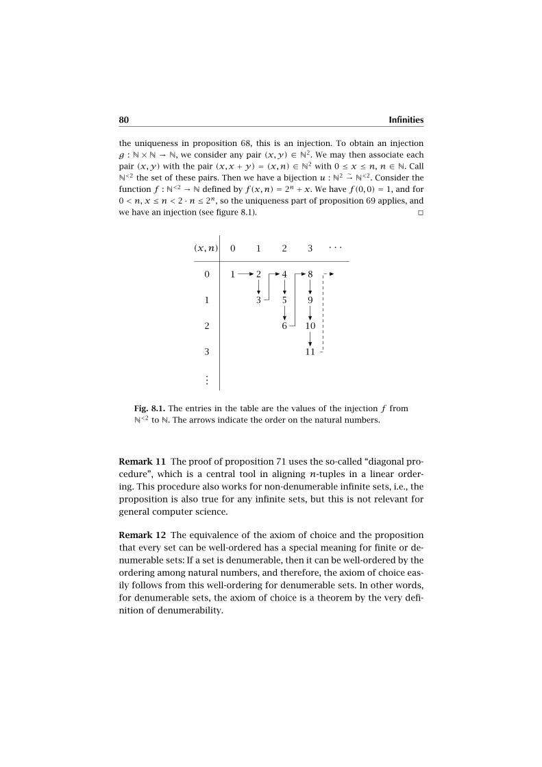
80 Infinities
the uniqueness in proposition 68, this is an injection. To obtain an injection
g : N × N → N, we consider any pair (x,y) ∈ N2. We may then associate each
pair (x,y) with the pair (x,x + y) = (x,n) ∈ N2 with 0 ≤ x ≤ n, n ∈ N. Call
N<2 the set of these pairs. Then we have a bijection u : N2 ∼→ N<2. Consider the
function f : N<2 → N defined by f(x,n) = 2n + x. We have f(0,0) = 1, and for
0 < n, x ≤ n < 2 ·n ≤ 2n, so the uniqueness part of proposition 69 applies, and
we have an injection (see figure 8.1). �
(x,n) 0 1 2 3 · · ·
0
1
2
3
...
1 2
3
4
5
6
8
9
10
11
Fig. 8.1. The entries in the table are the values of the injection f from
N<2 to N. The arrows indicate the order on the natural numbers.
Remark 11 The proof of proposition 71 uses the so-called “diagonal pro-
cedure”, which is a central tool in aligning n-tuples in a linear order-
ing. This procedure also works for non-denumerable infinite sets, i.e., the
proposition is also true for any infinite sets, but this is not relevant for
general computer science.
Remark 12 The equivalence of the axiom of choice and the proposition
that every set can be well-ordered has a special meaning for finite or de-
numerable sets: If a set is denumerable, then it can be well-ordered by the
ordering among natural numbers, and therefore, the axiom of choice eas-
ily follows from this well-ordering for denumerable sets. In other words,
for denumerable sets, the axiom of choice is a theorem by the very defi-
nition of denumerability.
CHAPTER 9
The Classical Number
Domains Z, Q, R, and C
This chapter is the recompensation for the abstract initialization of math-
ematics: it will give us all the central number domains as they are con-
structed from the natural numbers. In general, there are different meth-
ods for the construction of the same number domains. We have decided
to present the most direct methods which also lead to effective represen-
tations of numbers in computer environments.
First, the domain Z of integer numbers is constructed from natural num-
bersN, then rational numbers or fractionsQ from integers, and real num-
bers (also called decimal numbers in a special representation) from ratio-
nal numbers. This process culminates in the building of complex num-
bers from real numbers. These examples are also very important for the
understanding of subsequent chapters on algebra.
Basically, the construction of new number domains is motivated by the
absence of many operations one would like to apply to numbers. For
example, it is in general not possible to solv the domain of natural num-
bers. Moreover, we do not have any possibility to model most of the com-
mon geometric objects such as lines. Finally, non-linear equations such
as a2 = b cannot be solved.
Mathematics must supply tools that help us understand the solution
spaces for such problems. The set-theoretic approach has provided us
with the construction of numbers, and we are now ready to find solu-
tions to the aforementioned problems.
82 The Classical Number Domains Z, Q, R, and C
9.1 Integers Z
We have seen that the equation a+x = b for natural numbers has exactly
one solution in the case a ≤ b, we call it b − a. But for a > b, such a
solution does not exist within the domain of natural numbers. Integer
numbers, however, can solve this problem.
Lemma 72 Consider the relation R among pairs (a, b), (p, q) ∈ N2, de-
fined by “(a, b)R(p, q) iff a+ q = b + p”.
(i) The relation R is an equivalence relation.
(ii) A pair (a, b) ∈ N2 with a ≥ b is equivalent to (a− b,0), whereas a
pair (a, b) ∈ N2 with a < b is equivalent to (0, b − a).(iii) Two pairs (x,0), (y,0), or (0, x), (0, y), respectively, are equivalent
iff x = y . Two pairs (x,0), (0, y) are equivalent iff x = y = 0.
Proof The relation R is reflexive since (a, b)R(a, b) iff a + b = b + a by
the commutativity of addition. It is symmetric for the same reason. And if
(a, b)R(p, q) and (p, q)R(r , s), then a + q = b + p and p + s = q + r , whence
a+q+p+s = b+p+q+r , but then we may cancel p+q and obtain the desired
equality a+ s = b+ r . The other claims follow immediately from equivalence of
ordered pairs. �
Definition 39 The set N2/R is denoted by Z, its elements [a, b] are called
integers. Each integer is uniquely represented by either [a,0] for a ∈ N,
or by [0, b], b ∈ N−{0}. We identify the former class [a,0] with its unique
associated natural number a, and the latter class [0, b] with the uniquely
determined natural number b, together with a minus sign, i.e., by −b.
The numbers [a,0] with a ≠ 0 are called the positive integers, while the
numbers −b, b ≠ 0 are called the negative integers. The meeting point
between these number types is the number 0 = −0 (zero) which is neither
positive nor negative.
The linear ordering on the natural numbers is extended to the integers by
the rule that [a,0] < [c,0] iff a < c, and [0, a] < [0, c], i.e., −a < −c iff
a > c. Further, we set [a,0] > [0, b], i.e., a > −b for all natural b ≠ 0
and natural a. We finally set |[a,0]| = a and |[0, b]| = b and call this the
absolute value of the integer.
If x = [a, b] is an integer, we further denote by −x the integer [b,a]
and call it the additive inverse. This definition evidently generalizes the
convention −c = [0, c]. We also write a− b for a+ (−b).
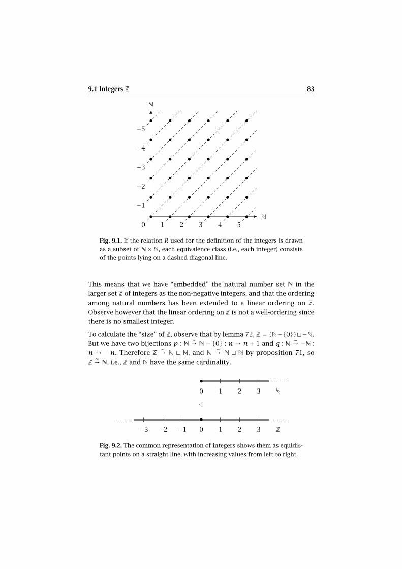
9.1 Integers Z 83
N
N
0 1 2 3 4 5
−5
−4
−3
−2
−1
Fig. 9.1. If the relation R used for the definition of the integers is drawn
as a subset of N × N, each equivalence class (i.e., each integer) consists
of the points lying on a dashed diagonal line.
This means that we have “embedded” the natural number set N in the
larger set Z of integers as the non-negative integers, and that the ordering
among natural numbers has been extended to a linear ordering on Z.
Observe however that the linear ordering on Z is not a well-ordering since
there is no smallest integer.
To calculate the “size” of Z, observe that by lemma 72, Z = (N−{0})t−N.
But we have two bijections p : N∼→ N− {0} : n , n+ 1 and q : N
∼→ −N :
n , −n. Therefore Z∼→ N t N, and N
∼→ N t N by proposition 71, so
Z∼→ N, i.e., Z and N have the same cardinality.
0 1 2 3 N
⊂
−3 −2 −1 0 1 2 3 Z
Fig. 9.2. The common representation of integers shows them as equidis-
tant points on a straight line, with increasing values from left to right.
84 The Classical Number Domains Z, Q, R, and C
Next, we will create an arithmetic on Z which extends the arithmetic on
the natural numbers. The following technique for defining addition of in-
tegers is a prototype of the definition of functions on equivalence classes:
One defines these functions on elements (representatives) of such equiv-
alence classes and then shows that the result is in fact not a function
of the representative, but only of the class as a such. If a definition on
representatives works in this sense, one says that the function is well
defined.
Definition 40 Given two integers [a, b] and [c, d], their sum is defined
by [a, b] + [c, d] = [a + c, b + d], i.e., “factor-wise”. This function is well
defined.
In order to show that this function is well defined, we have to make sure
that it is independent of the specific representatives of the equivalence
classes. So assume that [a, b] = [x,y], and [c, d] = [r , s], i.e., a + y =b+x, and c+s = d+r , respectively. We have to show that [a+c, b+d] =[x + r ,y + s], i.e., a+ c +y + s = b + d+ x + r . But
a+ c +y + s = a+y + c + s= b + x + c + s= b + x + d+ r= b + d+ x + r ,
where the properties of commutativity and associativity of natural num-
bers have been used. Thus the addition of integers is indeed well defined.
Sorite 73 Let Z be provided with the addition + : Z× Z→ Z, and let a,b, c
be any integers. Then we have these properties.
(i) (Associativity) (a+ b)+ c = a+ (b + c) = a+ b + c,(ii) (Commutativity) a+ b = b + a,
(iii) (Additive neutral element) a+ 0 = a,
(iv) (Additive inverse element) a− a = 0,
(v) (Extension of natural arithmetic) If a,b ∈ N, then [a + b,0] =[a,0] + [b,0], i.e., it amounts to the same if we add two natural
numbers a and b or the corresponding non-negative integers, also
denoted by a and b.
(vi) (Solution of equations) The equation a+ x = b in the “unknown” x
has exactly one integer number solution x, i.e., x = b − a.
9.1 Integers Z 85
Proof (i), (ii), (iii) Associativity, commutativity, and the neutrality of 0 immedi-
ately follows from associativity for natural numbers and the factor-wise defini-
tion of addition.
(iv) For a = [u,v], we have a−a = a+(−a) = [u,v]+[v,u] = [u+v,u+v] = 0.
The rest is immediate from the definitions. �
Definition 41 Let (ai)i=0,...n be a sequence of integers. Then the sum of
this sequence is defined by
n = 0 :∑
i=0,...n
ai = a0,
n > 0 :∑
i=0,...n
ai = ∑
i=0,...n−1
ai
+ an.
It is also possible to extend the multiplication operation defined on N to
the integers. The definition is again one by representatives of equivalence
classes [a, b]. To understand the definition, we first observe that a class
[a, b] is equal to the difference a− b of natural numbers with the above
identification. In fact, [a, b] = [a,0]+ [0, b] = a+ (−b) = a−b. So, if we
want to extend the arithmetic on the natural numbers, we should try to
observe the hoped for and given rules, and thereby get the extension. So
we should have [a, b] · [c, d] = (a− b) · (c − d) = ac + bd− ad− bc =[ac + bd,ad+ bc]. This motivates the following definition:
Definition 42 Given two integers [a, b] and [c, d], their product is defined
by [a, b] · [c, d] = [ac + bd,ad+ bc]. This function is well defined.
Sorite 74 Let a,b, c be three integers. We have these rules for their multi-
plication.
(i) (Associativity) (a · b) · c = a · (b · c) = a · b · c,(ii) (Commutativity) a · b = b · a,
(iii) (Multiplicative neutral element) the element 1 = [1,0] is neutral for
multiplication, a · 1 = a,
(iv) (Zero and negative multiplication) a ·0 = 0 and a ·(−b) = −(a ·b),(v) (Distributivity) a · (b + c) = a · b + a · c,
(vi) (Integrity) If a,b ≠ 0, then a · b ≠ 0,
(vii) (Additive monotony) if a < b, then a+ c < b + c,(viii) (Multiplicative monotony) if a < b and 0 < c, then a · c < b · c,

86 The Classical Number Domains Z, Q, R, and C
(ix) (Extension of natural arithmetic) For two natural numbers a and b,
we have [a·b,0] = [a,0]·[b,0]. This allows complete identification
of the natural numbers as a subdomain of the integers, with respect
to addition and multiplication.
Proof Statements (i) through (v) and (ix) are straightforward and yield good
exercises for the reader.
(vi) If a = [r , s] and b = [u,v], then the hypothesis means r ≠ s and u ≠ v .
Suppose that r > s and u > v . Then a = [r − s,0] and b = [u − v,0], with
the notation of differences of natural numbers as defined at the beginning of
this section. But then a · b = [(r − s) · (u − v),0] ≠ [0,0]. The other cases
r < s,u < v , or r < s,u > v , or r > s,u < v are similar.
(vii) First suppose that r ≥ s and u ≥ v , and let a = [r , s] = [r − s,0] and
b = [u,v] = [u−v,0]. Then a < bmeans e = r−s < f = u−v . So for c = [g,h],we have a+c = [e+g,h] and b+c = [f+g,h]. We may suppose that either h or g
is zero. If h = 0, then e+g < f+g implies a+c = [e+g,0] < [f+g,0] = b+c. Else
we have a+c = [e,h] and b+c = [f ,h]. Suppose that h ≤ e. Then e−h < f −h,
whence a + c = [e,h] = [e − h,0] < [f − h,0] = b + c. If e < h ≤ f , then
a + c = [e,h] = [0, h − e] < [f − h,0] = b + c. If e, f < h, then h − e > h − f ,
and then a+ c = [e,h] = [0, h− e] < [0, h− f]. The other cases r < s,u < v , or
r < s,u > v , or r > s,u < v are similar.
(viii) If 0 ≤ a < b, we are done since this is the case for natural numbers, already
proven in sorite 66. Else if a < b < 0, then we have 0 < (−b) < (−a), and then
by the previous case, (−b) · c < (−a) · c, whence, −(−a) · c < −(−b) · c, but
−(−a) · c = a · c,−(−b) · c = b · c, whence the statement in this case. Else if
a ≤ 0 < b, then a · c ≤ 0 < b · c. �
We are now capable of adding and subtracting any two integers, and of
solving an equation of the type a + x = b. But equations of the type
a · x = b have no integer solution in general, for example, there is no
integer x such that 2 · x = 3.
Definition 43 If a and b are two integers, we say that a divides b iff there
is an integer c with a · c = b. We then write a|b.
Exercise 30 For any integer b, we have b|b, −b|b, 1|b, and −1|b.
Definition 44 If b ≠ ±1 is such that it is divided only by ±b, 1 and −1,
then we call b a prime integer.
We shall deal with the prime numbers in chapter 16. For the moment, we
have the following exercise concerning prime decomposition of integers.
For this we also need the product of a finite sequence of integers, i.e.,

9.2 Rationals Q 87
Definition 45 Let (ai)i=0,...n be a sequence of integers. Then the product
of this sequence is defined by
n = 0 :∏
i=0,...n
ai = a0,
n > 0 :∏
i=0,...n
ai = ∏
i=0,...n−1
ai
· an.
Exercise 31 Show that every non-zero integer a ≠ ±1 has a multiplica-
tive decomposition a = σ · ∏i pi where∏i pi is a product of positive
primes pi and σ = ±1.
Notation 8 We shall henceforth also write ab instead of a · b if no confu-
sion is possible.
Proposition 75 (Triangle Inequality) If a and b are two integers, then we
have the triangle inequality:
|a+ b| ≤ |a| + |b|.
Exercise 32 Give a proof of proposition 75 by distinction of all possible
cases for non-negative or negative a,b.
9.2 Rationals Q
The construction of the rational numbers is very similar to the procedure
we have used for the construction of the integers. The main difference is
that the underlying building principle is multiplication instead of addi-
tion. We denote by Z∗ the set Z− {0}.
Lemma 76 On the set Z × Z∗, the relation R, defined by “(a, b)R(c, d) iff
ad = bc”, is an equivalence relation.
Proof This is an exercise for the reader. �
Definition 46 The set (Z× Z∗)/R of equivalence classes for the relation R
defined in lemma 76 is denoted by Q. Its elements, the classes [a, b], are
called rational numbers and are denoted byab or a/b. The (non uniquely
determined) number a is called the numerator, whereas the (non uniquely
determined) number b is called the denominator of the rational number
88 The Classical Number Domains Z, Q, R, and C
ab . Numerator and denominator are only defined relative to a selected rep-
resentative of the rational number.
Before we develop the arithmetic operations onQ, let us verify that again,
the integers are embedded in the rationals. In fact, we may identify an
integer a with its fractional representation a1 , and easily verify that a1 = b
1
iff a = b.
Here is the arithmetic construction:
Definition 47 Letab and
cd be two rationals. Then we define
ab + c
d = ad+bcbd
ab · cd = ac
bd .
We further set −ab = −ab for the additive inverse of
ab . If a ≠ 0, we set(
ab
)−1 = ba , the latter being the multiplicative inverse of a
b . These opera-
tions are all well defined.
In order to manage comparison between rational numbers, we need the
following exercise.
Exercise 33 If ab and cd are rational numbers, show that one may always
find numerators and denominators such that b = d (common denomina-
tor) and 0 < b.
Definition 48 Ifab and
cd are rational numbers, we have the (well defined)
relationab <
cd iff a < c, where we suppose that we have a common positive
denominator 0 < b = d.
Sorite 77 Letab ,cd ,ef be rational numbers. Then these rules hold.
(i) (Additive associativity) (ab + cd)+ e
f = ab + ( cd + e
f ) = ab + c
d + ef
(ii) (Additive commutativity)ab + c
d = cd + a
b
(iii) (Additive neutral element)ab + 0
1 = ab
(iv) (Additive inverse element)ab + −a
b = 01
(v) (Multiplicative associativity) (ab · cd) · ef = ab · ( cd · ef ) = a
b · cd · ef(vi) (Multiplicative commutativity)
ab · cd = c
d · ab(vii) (Multiplicative neutral element)
ab · 1
1 = ab
(viii) (Multiplicative inverse element) If a,b ≠ 0, thenab · ba = 1
1
9.2 Rationals Q 89
(ix) (Distributivity)ab · ( cd + e
f ) = ab · cd + a
b · ef(x) (Linear ordering) The relation< among rational numbers is a linear
ordering. Its restriction to the integersa1 induces the given linear
ordering among integers.
(xi) (Additive monotony) Ifab <
cd , then
ab + e
f <cd + e
f .
(xii) (Multiplicative monotony) Ifab <
cd and
01 <
ef , then
ab · ef < c
d · ef .
(xiii) (Archimedean ordering) For any two positive rational numbersab
andcd there is a natural number n such that
n1 · ab > c
d .
Proof Everything here is straightforward once one has shown that in fact ab<
cd
is well defined. For then we may calculate everything on (common) positive
denominators and thereby reduce the problem to the integers, where we have
already established these properties. So let ab< c
b, and b be positive. Suppose
that ab= a′
b′ and cb= c′
b′ . We know a < c. Then ab′ = ba′ and cb′ = c′b, and
therefore a′b = b′a < b′c = c′b, whence a′ < c′, since b is positive. �
Given the complete compatibility of original natural numbers within inte-
gers, and the complete compatibility of integers within rational numbers,
we also “abuse” the injections
N→ Z→ Q
and treat them as inclusions, in the sense that
• a natural number is denoted by n rather than by the equivalence class
[n,0] in Z,
• an integer is denoted by z rather than by the equivalence class z1 in Q.
Definition 49 If a rational number x is represented by x = ab , then we
define its absolute value |x| by |x| = |a||b| . This is a well-defined definition.
Exercise 34 Prove that |x| is well defined. An alternative definition is
this: |x| = x if 0 ≤ x, otherwise it is |x| = −x. Give a proof of this.
Proposition 78 (Triangle Inequality) If a and b are rational numbers,
then we have the triangle inequality:
|a+ b| ≤ |a| + |b|.
Exercise 35 Use proposition 75 to give a proof of proposition 78.
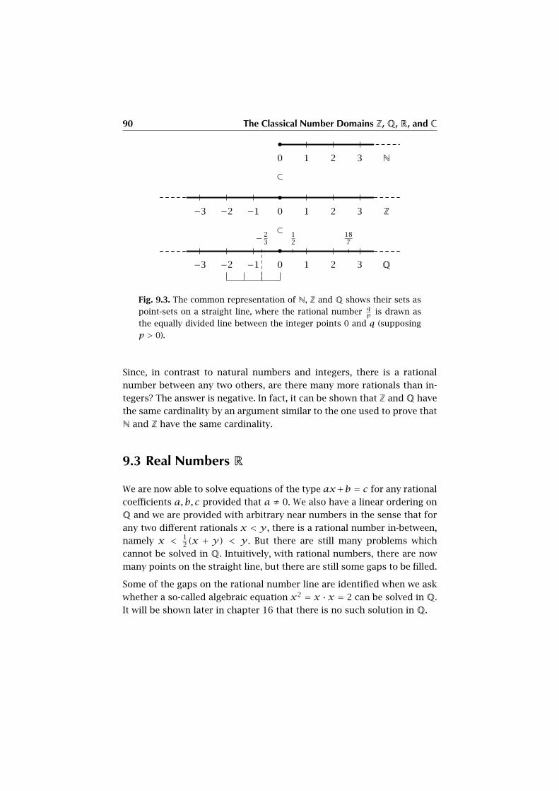
90 The Classical Number Domains Z, Q, R, and C
0 1 2 3 N
⊂
−3 −2 −1 0 1 2 3 Z
⊂
−3 −2 −1 0 1 2 3 Q
−23
12
187
Fig. 9.3. The common representation of N, Z and Q shows their sets as
point-sets on a straight line, where the rational number qp
is drawn as
the equally divided line between the integer points 0 and q (supposing
p > 0).
Since, in contrast to natural numbers and integers, there is a rational
number between any two others, are there many more rationals than in-
tegers? The answer is negative. In fact, it can be shown that Z and Q have
the same cardinality by an argument similar to the one used to prove that
N and Z have the same cardinality.
9.3 Real Numbers R
We are now able to solve equations of the type ax+b = c for any rational
coefficients a,b, c provided that a ≠ 0. We also have a linear ordering on
Q and we are provided with arbitrary near numbers in the sense that for
any two different rationals x < y , there is a rational number in-between,
namely x < 12(x + y) < y . But there are still many problems which
cannot be solved in Q. Intuitively, with rational numbers, there are now
many points on the straight line, but there are still some gaps to be filled.
Some of the gaps on the rational number line are identified when we ask
whether a so-called algebraic equation x2 = x ·x = 2 can be solved in Q.
It will be shown later in chapter 16 that there is no such solution in Q.
9.3 Real Numbers R 91
We recognize once again that in fact all our efforts in the construction of
more numbers originate in the problem of solving special equations in a
given number domain.
The real numbers are constructed from the rational numbers by an idea
which results from the observation that the search for a solution of x2 =2 yields rational numbers y and z such that y2 < 2 < z2 and |y − z| <1/n for any non-zero natural number n, in other words, y and z are
arbitrary near to each other. The point is that there is no rational number
which gives us a precise solution, nonetheless, we would like to invent
a number which solves the problem and in some sense is the “infinite
approximation” suggested by the rational approximations.
In order to extend the rationals to the reals, we need to formalize what we
vaguely described by “infinite approximation”. This definition goes back
to the French mathematician Augustin Cauchy (1789–1857).
Definition 50 A Cauchy sequence of rational numbers is a sequence
(ai)i∈N of rational numbers ai such that for any positive natural num-
ber L, there is an index number N such that whenever indexes n,m satisfy
N < n,m, then |an − am| < 1L .
The set of all Cauchy sequences is denoted by C.
Exercise 36 Every rational number r gives rise to the constant Cauchy
sequence e(r) = (ai)i which has ai = r for all indexes 0 ≤ i.The sequence (1/(i + 1))i∈N is a Cauchy sequence. More generally, any
sequence (a + ai)i is a Cauchy sequence if a is a rational number and if
(ai)i is a Cauchy sequence.
A sequence of rational numbers (ai)i is said to converge to a rational
number a if for any positive natural number L, there is an index N such
that n > N implies |an − a| < 1L .
Show that a convergent sequence is a Cauchy sequence, and that the ratio-
nal number to which it converges is uniquely determined. We then write
limi→∞ ai = a. The sign∞means “infinity”, but it has no precise meaning
when used without a determined context, such as limn→∞.
Definition 51 A zero sequence is a Cauchy sequence (ai)i which con-
verges to 0:
limi→∞
ai = 0.
92 The Classical Number Domains Z, Q, R, and C
The zero sequences are those sequences which we would like to forget
about. To develop this idea, we begin with the following definition.
Definition 52 If (ai)i and (bi)i are sequences of rational numbers, their
sum is defined by
(ai)i + (bi)i = (ai + bi)i,and their product is defined by
(ai)i · (bi)i = (ai · bi)i.
Proposition 79 The following properties hold for sequences of rational
numbers:
(i) If (ai)i and (bi)i are Cauchy sequences, then so are their sum and
product.
(ii) If (ai)i and (bi)i are zero sequences, then so is their sum.
(iii) If (ai)i is a zero sequence and if (bi)i is a Cauchy sequence, then
their product is a zero sequence.
Proof Let (ai)i and (bi)i be Cauchy sequences. Given any positive natural
number L, there is a common natural number N such that n,m > N implies
|an − am| < 12L and |bn − bm| < 1
2L if n,m > N. Then
|(an + bn)− (am + bm)| = |(an − am)+ (bn − bm)|≤ |an − am| + |bn − bm|< 1
2L + 12L
= 1L
by the triangle inequality. Further
|(an · bn)− (am · bm)| = |(an · bn)− (an · bm)+ (an · bm)− (am · bm)|= |(an · (bn − bm)+ (an − am) · bm)|≤ |an · (bn − bm)| + |(an − am) · bm|= |an| · |bn − bm| + |an − am| · |bm|< (|an| + |bm|) 1
L
if n,m > N. Now, |an| = |(an − aN+1) + aN+1| ≤ 1L+ |aN+1| if n > N. Also
|bm| ≤ 1L+ |bN+1| if m > N. So, |(an · bn) − (am · bm)| ≤ kN · 1
Lif n,m > N,
where kN is a positive constant which is a function of N. Now, select N ′ such that
|an−am| < 1kNL
for n,m > N′ then we have |(an ·bn)−(am ·bm)| ≤ kN · 1kNL
= 1L
for n,m > N′.
9.3 Real Numbers R 93
If (ai)i and (bi)i converge to 0, let N be such that |an|, |bn| < 12L for n > N.
Then |an + bn| ≤ |an| + |bn| < 12L + 1
2L = 1L
for n > N.
Let (ai)i and (bi)i be two Cauchy sequences such that (ai)i converges to 0.
From the previous discussion we know that there is a positive constant k such
that |bn| < k for all n. Now, let N be such that |an| < 1kL
for all n > N. Then
|an · bn| = |an| · |bn| < k · 1kL= 1L
for n > N. �
The properties (ii) and (iii) of the set O of zero sequences make O a so-
called ideal. This is an important structure in algebra, we come back to
its systematic discussion in chapter 15. We are now ready to define real
numbers.
Lemma 80 The binary relation R on C defined by “(ai)iR(bi)i iff (ai)i −(bi)i = (ai − bi)i is a zero sequence” is an equivalence relation.
Proof Clearly, R is reflexive and symmetric. Let (ai)i, (bi)i, (ci)i be Cauchy se-
quences such that (ai)iR(bi)i and (bi)iR(ci)i. Then |an − cn| = |an − bn + bn −cn| ≤ |an−bn|+|bn−cn| < 1
Lfor n > N if N is such that |an−bn|, |bn−cn| < 1
2L
for n > N. �
Definition 53 The set C/R of equivalence classes under the relation R de-
fined in lemma 80 is denoted by R. Its elements are called real numbers.
Lemma 81 The equivalence class (the real number) of a Cauchy sequence
(ai)i is given by the “coset” of the ideal O, i.e., [(ai)i] = {(ai)i + (ci)i |(ci)i ∈ O} = (ai)i +O.
Proof If (ai)i and (bi)i are equivalent, then by definition (ai)i = (bi)i + ((ai)i−(bi)i), and (ai)i − (bi)i ∈ O. Conversely, if (ai)i = (bi)i + (oi)i, (oi)i ∈ O, then
(ai)iR(bi)i by the definition of R. �
Lemma 82 We have an injection e : Q → R defined by e(a) = (a)i +O.
Exercise 37 Give a proof of lemma 82.
We now want to develop the arithmetics on R, and we want to show that
the purpose of this construction is effectively achieved.
Lemma 83 Let (ai)i, (bi)i, (ci)i be Cauchy sequences of rational numbers.
(i) If (ai)i, (bi)i are equivalent, then so are (ai)i + (ci)i, (bi)i + (ci)i.(ii) If (ai)i, (bi)i are equivalent, then so are (ai)i · (ci)i, (bi)i · (ci)i.

94 The Classical Number Domains Z, Q, R, and C
Proof (i) In fact, ((ai)i + (ci)i) − ((bi)i + (ci)i) = (ai − bi)i, which is a zero
sequence.
(ii) Similarly, ((ai)i·(ci)i)−((bi)i·(ci)i) = ((ai−bi)i)(ci)i, but by proposition 79
this is a zero sequence. �
This enables the definition of addition and multiplication of real num-
bers:
Definition 54 If (ai)i + O and (bi)i + O are two real numbers, then we
define
((ai)i +O)+ ((bi)i +O) = (ai + bi)i +O((ai)i +O) · ((bi)i +O) = (ai · bi)i +O.
By lemma 83, this definition is independent of the representative Cauchy
sequences, i.e., it is well-defined.
Evidently, these operations, when restricted to the rational numbers, em-
bedded via e(r), r ∈ Q, as above, yield exactly the operations on the
rationals, i.e., e(r + s) = e(r) + e(s) and e(r · s) = e(r) · e(s). We there-
fore also use the rational numbers r instead of e(r) when working in R.
If x = (ai)i+O, we write −x for (−ai)i+O and call it the additive inverse
or negative of x.
The arithmetic properties of these operations on R are collected in the
following sorite:
Sorite 84 Let x,y, z be real numbers.
(i) (Additive associativity) (x +y)+ z = x + (y + z) = x +y + z(ii) (Additive commutativity) x +y = y + x(iii) (Additive neutral element) The rational zero 0 is also the additive
neutral element of the reals, i.e., x + 0 = x.
(iv) (Additive inverse element) x + (−x) = 0
(v) (Multiplicative associativity) (x ·y) · z = x · (y · z) = x ·y · z(vi) (Multiplicative commutativity) x ·y = y · x(vii) (Multiplicative neutral element) The rational unity 1 is also the mul-
tiplicative neutral element of the reals, i.e., x · 1 = x.
(viii) (Multiplicative inverse element) If x ≠ 0, then there is exactly one
multiplicative inverse x−1, i.e., x · x−1 = 1, more precisely, there
exists in this case a Cauchy sequence (ai)i representing x and such
9.3 Real Numbers R 95
that ai ≠ 0 for all i, and we may represent x−1 by the Cauchy
sequence (a−1i )i.
(ix) (Distributivity) x · (y + z) = x ·y + x · zProof (i) through (vii) as well as (ix) are straightforward, because all the relevant
operations are defined factor-wise on the sequence members (definition 54).
As to (viii), since (ai)i does not converge to zero, there is a positive natural
L such that for every N there is n > N with |an| ≥ 1L. Choose N such that
|an − am| < 12L for all n,m > N. Fix n > N such that |an| ≥ 1
Las above. Then
|am| ≥ |an| − |an − am| ≥ 1L− 1
2L = 12L > 0 for n,m > N. Therefore (ai)i is
equivalent to a sequence (a′i)i without zero members, more precisely: there is I
such that a′i = ai for i > I. Then evidently the sequence (1/a′i)i is the inverse
of (ai)i. The uniqueness of the inverse follows from the purely formal fact that
x · y = x · y ′ = 1 implies y = 1 · y = (y · x) · y = y · (x · y) = y · (x · y ′) =(y · x) ·y ′ = 1 ·y ′ = y ′. �
Corollary 85 If a,b, c are real numbers such that a ≠ 0, then the equation
ax + b = c has exactly one solution x.
This means that we have “saved” the algebraic properties of Q to R. But
we wanted more than that. Let us first look for the linear ordering struc-
ture on R.
Definition 55 A real number x = (ai)i +O is called positive iff there is a
rational number ε > 0 such that ai > ε for all but a finite set of indexes.
This property is well defined. We set x < y for two real numbers x and y
iff y − x is positive. In particular, x is positive iff x > 0.
Proposition 86 The relation < on R from definition 55 defines a linear
ordering. The set R is the disjoint union of the subset R+ of positive real
numbers, the subset R− = −R+ = {−x | x ∈ R+} of negative real num-
bers, and the singleton set {0}. We have
(i) R+ +R+ = {x +y | x,y ∈ R+} = R+,
(ii) R+ ·R+ = {x ·y | x,y ∈ R+} = R+,
(iii) R− +R− = {x +y | x,y ∈ R−} = R−,
(iv) R− ·R− = {(−x) · (−y) | x,y ∈ R+} = R+,
(v) R+ +R− = {x −y | x,y ∈ R+} = R ,
(vi) R+ ·R− = {x · (−y) | x,y ∈ R+} = R−,
(vii) (Monotony of addition) if x,y, z are real numbers with x < y , then
x + z < y + z,

96 The Classical Number Domains Z, Q, R, and C
(viii) (Monotony of multiplication) if x,y, z are real numbers with x < y
and 0 < z, then xz < yz,
(ix) (Archimedean property) if x and y are positive real numbers, there
is a natural number N such that y < Nx,
(x) (Density of rationals in reals) if ε > 0 is a positive real number, then
there is a rational number ρ with 0 < ρ < ε.
Proof Let us first show that < is antisymmetric. If x < y , then y − x is repre-
sented by a sequence (ai)i with ai > ε for a positive rational ε. Then x − y is
represented by (−ai)i, and −ai < ε < 0 for all but a finite set of indexes. If this
were equivalent to a sequence (bi)i with bi > ε′ > 0 except for a finite number of
indexes, then bi− (−ai) = bi+ai > ε+ ε′ could not be a zero sequence. Whence
antisymmetry.
Also, if y − x is represented by (ai)i with ai > ε and z − y is represented by
(bi)i with bi > ε′ for all but a finite number of indexes, then z−x = z−y+y−xis represented by (ai)i + (bi)i = (ai + bi)i, and ai + bi > ε + ε′ > 0 for all but a
finite number of indexes, whence transitivity. Finally, if x ≠ y , then x − y ≠ 0.
By the same argument as used in the previous proof, if (di)i represents x − y ,
then there is a positive rational ε and N, such that |dn| > ε for n > N. But since
(di)i is a Cauchy sequence, too, the differences |dn−dm| become arbitrary small
for large n and m. So either dn is positive or negative, but not both, for large
n, and therefore x − y is either positive or negative. This immediately entails
statements (i) through (viii).
(ix) If x is represented by (ai)i and y is represented by (bi)i, then there is a
positive rational ε and an index M such that an, bn > ε for n > M . But since
(bi)i is a Cauchy sequence, there is also a positive δ and index M ′ such that
bn < δ for n > M ′, and we may take the larger of M and M ′ and then suppose
thatM = M ′ for our two conditions. Then, sinceQ has the Archimedean ordering
property by sorite 77, there is a natural N such that N · ε > 2 · δ. Then we have
N · an > N · ε > 2 · δ > δ > bn for n > M , whence N · an − bn > δ > 0, whence
the claim.
(x) If the real number ε > 0 is represented by a Cauchy sequence (ei)i, then, by
the very definition of positivity, there is a positive rational number δ such that
ei > δ for all but a finite number of indexes. But then ei − δ2 >
δ2 for all but a
finite number of indexes, and ρ = δ2 is sought-after rational number. �
Definition 56 The absolute value |a| of a real number a is a if it is non-
negative, and −a else.
Proposition 87 (Triangle Inequality) If a and b are two real numbers,
then we have the triangle inequality:
9.3 Real Numbers R 97
|a+ b| ≤ |a| + |b|.
Proof Observe that, if a is represented by a Cauchy sequence (ai)i, then |a|is represented by (|ai|)i. Therefore, if b is represented by (bi)i, then |a + b| is
represented by (|ai + bi|)i, but by the triangle inequality for rationals, we have
|ai|+|bi| ≥ |ai+bi|, i.e., |a|+|b|−|a+b| is represented by (|ai|+|bi|−|ai+bi|)i,so it is not negative, thus |a| + |b| − |a+ b| ≥ 0, i.e., |a| + |b| ≥ |a+ b|. �
We now have a completely general criterion for convergence in R. Con-
vergence is to be defined entirely along the lines of the definition of con-
vergence for rational sequences.
Definition 57 A sequence (ai)i of real numbers is said to converge to a
real number a iff for every real ε > 0, there is an index N such that n > N
implies |an − a| < ε. Clearly, if such an a exists, then it is unique, and we
denote convergence to a by limi→∞ ai = a.
The sequence (ai)i is Cauchy, iff for every real number ε > 0, there is a
natural number N such that n,m > N implies that |an − am| < ε.
Proposition 88 (Convergence on R) A sequence (ai)i of real numbers
converges iff it is Cauchy.
Proof We omit the detailed proof since it is quite technical. However, the idea
of the proof is easily described: Let (ai)i be a Cauchy sequence of real numbers.
For each i > 0, there is a rational number ri such that |ai − ri| < 1i. This rational
number can be found as follows: Represent ai by a rational Cauchy sequence
(aij)j . Then there is an index Ii such that r , s > Ii implies |air − ais| < 1i. Then
take ri = air for any r > Ii. One then shows that (ri)i is Cauchy and that (ai)iconverges to (ri)i. �
This result entails a huge number of theorems about the existence of
special numbers. We just mention one particularly important concept.
Definition 58 (Upper Bound) A real number b is an upper bound of a set
A ⊂ R, if b ≥ a for all a ∈ A, in short b ≥ A.
Corollary 89 (Existence of Suprema) If A is a bounded, non-empty set,
i.e., if there is b ∈ R such that b ≥ A, then there is a uniquely determined
supremum or least upper bound s = sup(A), i.e., an upper bound s ≥ Asuch that for all t < s, there is a ∈ A with a > t.
Proof One first constructs a Cauchy sequence (ui)i of upper bounds ui of A as
follows: Let u0 be an existing upper bound and take a0 ∈ A. Then consider the
98 The Classical Number Domains Z, Q, R, and C
middle v1 = (a0 + u0)/2. If v1 is an upper bound, set u1 = v1, otherwise set
u1 = u0. In the first case, set a1 = a0, in the second case, there is a1 > v1; then
consider the pair a1, u1. In either case, their distance is half the first distance
|a0 − u0|. We now again take the middle of this interval, i.e., v2 = (a1 + u1)/2
and go on in the same way, i.e., defining a sequence of ui by induction, and
always taking the smallest possible alternative. This is a Cauchy sequence since
the intervals are divided by 2 in each step. Further, the limit u = limi→∞ui, which
exists according to proposition 88, is an upper bound, and there is no smaller
one, as is easily seen from the construction. The details are left to the reader. �
This corollary entails the following crucial fact:
Corollary 90 (Existence of n-th roots) Let a ≥ 0 be a non-negative real
number and n ≥ 1 a positive natural number, then there is exactly one
number b ≥ 0 such that bn = a. This number is denoted by n√a or by a
1n ,
in the case of n = 2 one simply writes 2√a = √a.
Proof The cases n = 1 or a = 0 are clear, so suppose n > 1 and a > 0. Let A
be the set of all q, such that qn < a. This set is bounded since an > a. Take
b = sup(A). We claim that bn = a. Clearly bn ≤ a. Suppose that bn < a. Then
consider the following construction of a contradiction:
First we claim that for any d > 0 there is a natural number m such that (1 +1m)n < 1+d. We show this by induction on n. In the case n = 1 we have (1+ 1
m) <
1+ d, we choose m such that m > 1d
, which exists since d > 0.
Suppose that, for n, we have found M such that (1 + 1m)n < 1 + d
2 for m ≥ M .
Then, for n+1, (1+ 1m)n+1 = (1+ 1
m)(1+ 1
m)n < (1+ 1
m)(1+ d
2 ) = 1+ 1m+ d
2 + d2m .
We require 1+ 1m+ d
2 + d2m < 1+ d, but this is true if m> 1+ 2
d.
Next, replace b by b(1+ 1m) and then we ask for an m such that (b(1+ 1
m))n =
bn(1+ d) < a. But we find such an m by the fact that for any positive d, we can
find m such that (1 + 1m)n < 1 + d, and it suffices to take d < a/bn − 1, this
contradicts the supremum property of b, and we are done. �
Exercise 38 Show that for two a,b ≥ 0, we have n√a · b = n
√a · n
√b.
Definition 59 One can now introduce more general rational powers xq,
q ∈ Q of a positive real number x as follows. First, one defines x0 = 1,
then for a negative integer −n, one puts x−n = 1/xn. For q = n/m ∈ Qwith positive denominator m, one defines xn/m = (x1/m)n. One easily
checks that this definition does not depend on the fractional representation
of q.
9.3 Real Numbers R 99
Exercise 39 Prove that for two rational numbers p and q and for two
positive real numbers x and y , one has xp+q = xpxq, xpq = (xp)q, and
(xy)p = xpyp .
Exercise 40 Let a > 1 and x > 0 be real numbers. Show that the set
{q ∈ Q | there are two integers m,n,0 < n,
such that am ≤ xn and q =m/n}
is non-empty and bounded from above. Its supremum is called the loga-
rithm of x for basis a, and is denoted by loga(x). It is the fundament of
the construction of the exponential function and of the sine and cosine
functions.
The general shape of real numbers as equivalence classes of rational
Cauchy sequences is quite abstract and cannot, as such, be handled by
humans when calculating concrete cases, and a fortiori cannot be han-
dled by computers in hard- and software contexts. Therefore, one looks
for more explicit and concrete representations of real numbers. Here is
such a construction, which generalizes the b-adic representation of nat-
ural numbers discussed in chapter 7. We consider a natural base number
b > 1 and for an integer n the index set n] = {i | i ∈ Z and i ≤ n}. Let
(ai)i∈n] be a sequence of natural numbers with 0 ≤ ai < b and an ≠ 0.
Consider the partial sums Σj =∑i=n,n−1,n−2,...j aib
i for j ∈ n].
Lemma 91 The sequence (Σj)n] of partial sums as defined previously con-
verges to a real number which we denote by∑i∈n] aibi, and, when the
base b is clear, by
anan−1 . . . a0.a−1a−2a−3 . . . (9.1)
for non-negative n, or, if n < 0, by
0.00 . . . anan−1 . . . , (9.2)
i.e., we put zeros on positions −1, . . . n + 1 until the first non-zero co-
efficient an appears on position n. The number zero is simply denoted
by 0.0 or even 0. The dots are meant to represent the given coeffi-
cients. If the coefficients vanish after a finite number of indexes, we can
either stop the representation at the last non-vanishing coefficient am:
anan−1 . . . a0.a−1 . . . am+1am, or append any number of zeros, such as
anan−1 . . . am+1am000.
100 The Classical Number Domains Z, Q, R, and C
Proof Let us show that the differences |Σk − Σj| of the rational partial sums
become arbitrarily small for large k and j. We may suppose that j > k and then
have Σk − Σj = aj−1bj−1 + . . . akbk < bj + . . . bk+1 = bj(1+ b−1 + . . . bk+1−j). But
we have this quite general formula which is immediately checked by evaluation:
1+ b−1 + . . . b−r = (1− b−r−1)/(1− b) < 1/(1− b). And therefore 0 ≤ Σk − Σj <bj ·1/(1−b). But the right side converges to zero as j → −∞, and we are done. �
Definition 60 The representation of a real number in the forms (9.1)
or (9.2) is called the b-adic representation; in computer science, the syn-
onymous term b-ary is more common. For b = 2 it is called the binary
representation, for b = 10, the decimal representation, and for b = 16, it
is called the hexadecimal representation. The extension of the b-adic rep-
resentation to negative real numbers is defined by prepending the sign −.
This extended representation is also called b-adic representation.
Proposition 92 (Adic Representation) Given a base number b ∈ N, b >
1, every real number can be represented in the b-adic representation. The
representation is unique up to the following cases: If the coefficients ai are
smaller than b − 1 until index m, and equal to b − 1 from m − 1 until
infinity, then this number is equal to the number whose coefficients are
the old ones for i > m, while the coefficient at index m is am + 1, and all
lower coefficients vanish.
Proof We may evidently suppose that the real number to be represented is pos-
itive, the other cases can be deduced from this. We construct the representation
by induction as follows: Observe that we have bi > bj > 0 whenever i > j, i
and j being integers. Moreover, bi converges to 0 as i → −∞, and bi becomes
arbitrarily large if i→∞. Therefore, there is a unique j such that bj ≤ x < bj+1.
Within this interval of b powers there is a unique natural aj with 0 < aj < b
such that ajbj ≤ x < (aj + 1)bj . Consider the difference x′ = x − ajbj , then
we have 0 ≤ x′ < bj and there is a unique natural 0 ≤ aj−1 < b such that
aj−1bj−1 ≤ x′ < (aj−1 + 1)bj−1. Then x′′ = x′ − aj−1b
j−1 = x − ajbj − aj−1bj−1
has 0 ≤ x′′ < bj−1, and we may go on in this way, defining a b-adic number. It
is immediate that this number converges to x. The failure of uniqueness in the
case where one has b − 1 until infinity is left as an exercise to the reader. �
Example 22 In the decadic representation, the number 0.999 . . . with
a non-terminating sequence of 9s is equal to 1.0. Often, one writes
. . . am+1am in order to indicate that the coefficient is constant and equal
to am for all indexes m,m − 1,m − 2, . . . . Thus, in the binary represen-
tation, 0.1 equals 1.0.
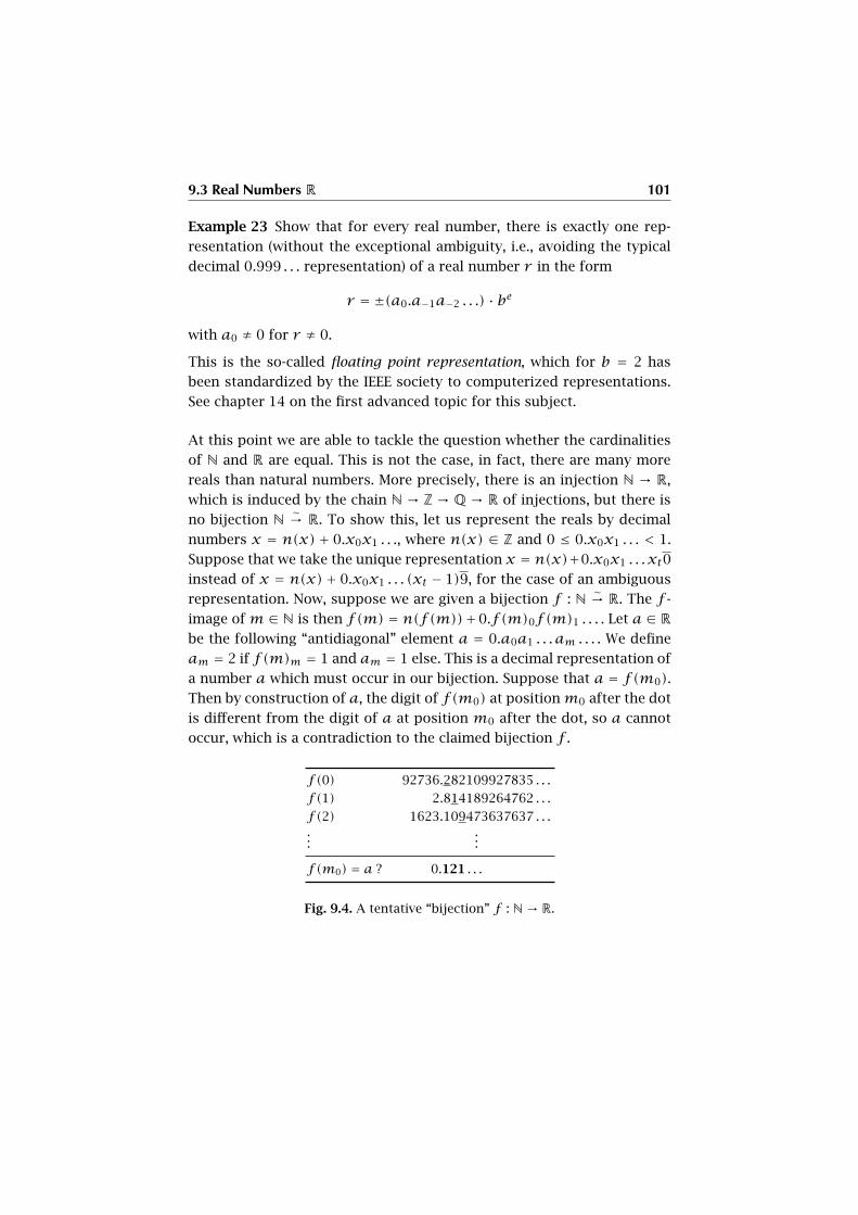
9.3 Real Numbers R 101
Example 23 Show that for every real number, there is exactly one rep-
resentation (without the exceptional ambiguity, i.e., avoiding the typical
decimal 0.999 . . . representation) of a real number r in the form
r = ±(a0.a−1a−2 . . .) · be
with a0 ≠ 0 for r ≠ 0.
This is the so-called floating point representation, which for b = 2 has
been standardized by the IEEE society to computerized representations.
See chapter 14 on the first advanced topic for this subject.
At this point we are able to tackle the question whether the cardinalities
of N and R are equal. This is not the case, in fact, there are many more
reals than natural numbers. More precisely, there is an injection N → R,
which is induced by the chain N → Z → Q → R of injections, but there is
no bijection N∼→ R. To show this, let us represent the reals by decimal
numbers x = n(x) + 0.x0x1 . . ., where n(x) ∈ Z and 0 ≤ 0.x0x1 . . . < 1.
Suppose that we take the unique representation x = n(x)+0.x0x1 . . . xt0
instead of x = n(x) + 0.x0x1 . . . (xt − 1)9, for the case of an ambiguous
representation. Now, suppose we are given a bijection f : N∼→ R. The f -
image ofm ∈ N is then f(m) = n(f(m))+0.f (m)0f(m)1 . . . . Let a ∈ Rbe the following “antidiagonal” element a = 0.a0a1 . . . am . . . . We define
am = 2 if f(m)m = 1 and am = 1 else. This is a decimal representation of
a number a which must occur in our bijection. Suppose that a = f(m0).
Then by construction of a, the digit of f(m0) at positionm0 after the dot
is different from the digit of a at position m0 after the dot, so a cannot
occur, which is a contradiction to the claimed bijection f .
f(0) 92736.282109927835 . . .
f (1) 2.814189264762 . . .
f (2) 1623.109473637637 . . ....
...
f(m0) = a ? 0.121 . . .
Fig. 9.4. A tentative “bijection” f : N→ R.
102 The Classical Number Domains Z, Q, R, and C
9.4 Complex Numbers C
The last number domain which we need in the general mathematical en-
vironment are the complex numbers. The theory that we have developed
so far enables us to solve equations such as ax + b = c, and we have
convergence of all Cauchy sequences, including the standard adic repre-
sentations. But there is still a strong deficiency: General equations cannot
be solved in R. More precisely, one can easily show that an equation of the
form ax3 +bx2 + cx +d = 0 with real coefficients a,b, c, d and a ≠ 0 al-
ways has a solution (a “root”) in R. But an equation with an even maximal
power of the unknown, such as ax4 + bx3 + cx2 +dx + e = 0, cannot be
solved in general. Two hundred years ago, mathematicians were search-
ing for a domain of numbers where the special equation x2 + 1 = 0 has
a solution. Evidently, such a solution does not exist in R since in R any
square is non-negative, and therefore x2 + 1 ≥ 1.
The solution was rigorously conceptualized by Carl Friedrich Gauss. In-
stead of working in R, he considers the plane R2 of pairs of real num-
bers. His trick is to give this set an arithmetic structure, i.e., addition
and multiplication, such that the existing R arithmetic and the entire
Cauchy sequence structure are embedded and such that we can effec-
tively solve the critical equation x2 + 1 = 0. But Gauss’ invention is
much deeper: It can be shown that in his construction, every equation
anxn + an−1x
n−1 + . . . + a1x + a0 = 0 has a solution, this is the funda-
mental theorem of algebra, see remark 22 in chapter 16. Therefore, the
solvability of that single equation x2 + 1 = 0 implies that we are done
once for all with this type of equation solving. The type of equation is
called polynomial equation, we shall come back to this structure in the
second part of the book (chapter 15).
Gauss’ complex numbers are defined as follows. We consider the Carte-
sian product R2, i.e., the set of ordered pairs (x,y) of real numbers.
When thinking of the arithmetical structure (addition, multiplication) on
R2, we denote this domain by C and call it the domain of complex num-
bers. Here are the two fundamental operations, addition and multiplica-
tion of complex numbers:
Definition 61 Given two complex numbers (x,y) and (u,v) ∈ C, we de-
fine the sum
(x,y)+ (u,v) = (x +u,y + v),
9.4 Complex Numbers C 103
while the product is defined by
(x,y) · (u,v) = (xu−yv,xv +yu).
Here is the sorite for this arithmetic structure:
Sorite 93 Let x,y, z be complex numbers, and denote 0 = (0,0) and 1 =(1,0). Then:
(i) (Additive associativity) We have (x+y)+z = x+(y+z) and denote
this number by x +y + z.
(ii) (Multiplicative associativity) We have (x · y) · z = x · (y · z) and
denote this number by x ·y ·z, or also xyz, if no confusion is likely.
(iii) (Commutativity) We have x +y = y + x and x ·y = y · x.
(iv) (Distributivity) We have x · (y + z) = x ·y + x · z.
(v) (Additive and multiplicative neutral elements) We have 0 + x = xand 1 · x = x.
(vi) If a ≠ 0, then every equation a · x = b has a unique solution; in
particular, the solution of a · x = 1, the multiplicative inverse of a,
is denoted by a−1. The solution of a+x = 0, the additive inverse (or
negative) of a, is denoted by −a.
Proof The statements (i) through (v) follow from the arithmetic properties of
reals.
(vi) Let a = (x,y) ≠ (0,0), Then x2 + y2 > 0. But then ( 1x2+y2 ,0) · (x,−y) ·
(x,y) = (1,0), so a−1 = ( 1x2+y2 ,0) · (x,−y) is an inverse of a. It is unique by an
argument already used in corresponding situations. If z and z′ are two inverses
of a, then z = z · 1 = z · (a · z′) = (z · a) · z′ = 1 · z′ = z′. �
The geometric view of Gauss is this: We have an injection R → C which
sends a real number a to the complex number (a,0). Similarly to the
embedding Q → R discussed above, all arithmetic operations, addition
and multiplication, “commute” with this embedding, i.e., (a + b,0) =(a,0) + (b,0) and (a · b,0) = (a,0) · (b,0). We therefore identify the
real number a with its image (a,0) in C. With this convention, denote
the complex number (0,1) by i, and call it the imaginary unit. Evidently,
i2 = −1. This means that in C, the equation x2+1 = 0 now has a solution,
namely x = i.Further, for a complex number x = (a, b), we write Re(x) = a and call it
the real part of x, similarly we write Im(x) = b and call it the imaginary
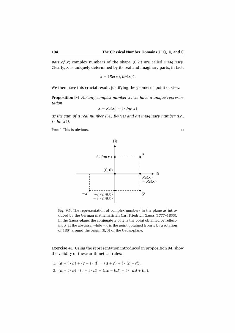
104 The Classical Number Domains Z, Q, R, and C
part of x; complex numbers of the shape (0, b) are called imaginary.
Clearly, x is uniquely determined by its real and imaginary parts, in fact:
x = (Re(x), Im(x)).
We then have this crucial result, justifying the geometric point of view:
Proposition 94 For any complex number x, we have a unique represen-
tation
x = Re(x)+ i · Im(x)
as the sum of a real number (i.e., Re(x)) and an imaginary number (i.e.,
i · Im(x)).
Proof This is obvious. �
iR
R
x
Re(x)= Re(x)
(0,0)
x−x −i · Im(x)= i · Im(x)
i · Im(x)
Fig. 9.5. The representation of complex numbers in the plane as intro-
duced by the German mathematician Carl Friedrich Gauss (1777–1855).
In the Gauss-plane, the conjugate x of x is the point obtained by reflect-
ing x at the abscissa, while −x is the point obtained from x by a rotation
of 180◦ around the origin (0,0) of the Gauss-plane.
Exercise 41 Using the representation introduced in proposition 94, show
the validity of these arithmetical rules:
1. (a+ i · b)+ (c + i · d) = (a+ c)+ i · (b + d),2. (a+ i · b) · (c + i · d) = (ac − bd)+ i · (ad+ bc).
9.4 Complex Numbers C 105
The complex numbers have a rich inner structure which is related to the
so-called conjugation.
Definition 62 The conjugation is a map C → C : x , x defined by x =Re(x)− i · Im(x), i.e., Re(x) = Re(x) and Im(x) = −Im(x).
The norm of a complex number x is defined by |x| = √x · x, which is a
non-negative real, since x · x = Re(x)2 + Im(x)2 ≥ 0.
Observe that the norm of a complex number x = a+ i ·b is the Euclidean
length of the vector (a, b) ∈ R2 known from high school.
Sorite 95 Let x,y ∈ C. Then
(i) x = x iff x ∈ R, and x = −x iff x is imaginary,
(ii) |x| = 0 iff x = 0,
(iii) Re(x) = x+x2 and Im(x) = x−x
2i ,
(iv) if x ≠ 0, then the multiplicative inverse of x is x−1 = |x|−2 · x,
(v) x = x; in particular, conjugation is a bijection,
(vi) x +y = x +y ,
(vii) x ·y = x ·y ,
(viii) if x is real, then |x| in the sense of real numbers coincides with |x| inthe sense of complex numbers, which justifies the common notation,
(ix) |x ·y| = |x| · |y|,(x) (Triangle inequality) |x +y| ≤ |x| + |y|.
Proof The only non-trivial statement is the triangle inequality. It suffices to show
that |x+y|2 ≤ (|x|+ |y|)2. This gives us the inequality yx+xy ≤ 2|x||y|, and
then, by putting a = xy , we get inequality a+ a ≤ |a| + |a| which is obvious by
simple explication of the coordinates of the complex number a. �
CHAPTER 10
Categories of Graphs
In this chapter, we introduce the concept of a graph. Note that, this is
homonymous with but really different from the already known concept
of a graph relation. Please do observe this historically grown ambiguity.
Of course, both concepts are related by the fact that they allude to some-
thing being drawn: The graph of a function is just what in nice cases
will be drawn as a graphical representation of that function, whereas
the other meaning is related to the graphical representation of assign-
ments between nodes of a processual assembly—the concrete situations
are completely different.
As a preliminary construction we need this setup: Given a set V , always
finite in this context, we have the Cartesian product V 2 = V × V . In ad-
dition we define the edge set as 2V = {a ⊂ V | 1 ≤ card(a) ≤ 2}. It
has this name because it parametrizes the set of all undirected lines, i.e.,
edges, including single points (“loop at x”), between any two elements of
V . We have the evident surjection |?| : V 2 → 2V : (x,y) , {x,y}, which
has a number of sections which we (somewhat ambiguously) denote by-→? : 2V → V2, i.e., |?| ◦ -→? = Id 2V .
Exercise 42 Give reasons for the existence of sections-→? of |?|.
We further denote by ?∗ : V2 → V2 : (x,y) , (y,x) the exchange bijec-
tion, and note that (x,y)∗∗ = (x,y).
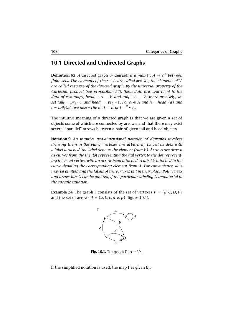
108 Categories of Graphs
10.1 Directed and Undirected Graphs
Definition 63 A directed graph or digraph is a map Γ : A → V 2 between
finite sets. The elements of the set A are called arrows, the elements of V
are called vertexes of the directed graph. By the universal property of the
Cartesian product (see proposition 57), these data are equivalent to the
data of two maps, headΓ : A → V and tailΓ : A → V ; more precisely, we
set tailΓ = pr1 ◦ Γ and headΓ = pr2 ◦ Γ . For a ∈ A and h = headΓ (a) and
t = tailΓ (a), we also write a : t → h or tañ h.
The intuitive meaning of a directed graph is that we are given a set of
objects some of which are connected by arrows, and that there may exist
several “parallel” arrows between a pair of given tail and head objects.
Notation 9 An intuitive two-dimensional notation of digraphs involves
drawing them in the plane: vertexes are arbitrarily placed as dots with
a label attached (the label denotes the element from V ). Arrows are drawn
as curves from the the dot representing the tail vertex to the dot represent-
ing the head vertex, with an arrow head attached. A label is attached to the
curve denoting the corresponding element from A. For convenience, dots
may be omitted and the labels of the vertexes put in their place. Both vertex
and arrow labels can be omitted, if the particular labeling is immaterial to
the specific situation.
Example 24 The graph Γ consists of the set of vertexes V = {B,C,D, F}and the set of arrows A = {a,b, c, d, e, g} (figure 10.1).
F B
C D
a
g
b
cd
e
Γ
Fig. 10.1. The graph Γ : A→ V 2.
If the simplified notation is used, the map Γ is given by:
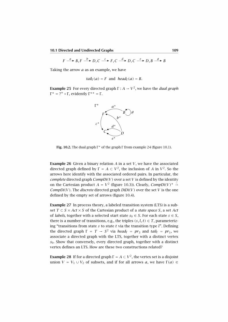
10.1 Directed and Undirected Graphs 109
Fañ B, F
bñ D,C
cñ F,C
dñ D,C
eñ D,B
gñ B
Taking the arrow a as an example, we have
tailΓ (a) = F and headΓ (a) = B.
Example 25 For every directed graph Γ : A→ V 2, we have the dual graph
Γ∗ = ?∗ ◦ Γ , evidently Γ∗∗ = Γ .
F B
C D
a∗
g
b∗
c∗d∗
e∗
Γ∗
Fig. 10.2. The dual graph Γ∗ of the graph Γ from example 24 (figure 10.1).
Example 26 Given a binary relation A in a set V , we have the associated
directed graph defined by Γ = A ⊂ V 2, the inclusion of A in V 2. So the
arrows here identify with the associated ordered pairs. In particular, the
complete directed graph CompDi(V) over a set V is defined by the identity
on the Cartesian product A = V 2 (figure 10.3)). Clearly, CompDi(V)∗ ∼→CompDi(V). The discrete directed graph DiDi(V) over the set V is the one
defined by the empty set of arrows (figure 10.4).
Example 27 In process theory, a labeled transition system (LTS) is a sub-
set T ⊂ S × Act × S of the Cartesian product of a state space S, a set Act
of labels, together with a selected start state s0 ∈ S. For each state s ∈ S,
there is a number of transitions, e.g., the triples (s, l, t) ∈ T , parameteriz-
ing “transitions from state s to state t via the transition type l”. Defining
the directed graph Γ = T → S2 via headΓ = pr3 and tailΓ = pr1, we
associate a directed graph with the LTS, together with a distinct vertex
s0. Show that conversely, every directed graph, together with a distinct
vertex defines an LTS. How are these two constructions related?
Example 28 If for a directed graph Γ = A ⊂ V 2, the vertex set is a disjoint
union V = V1 ∪ V2 of subsets, and if for all arrows a, we have Γ(a) ∈
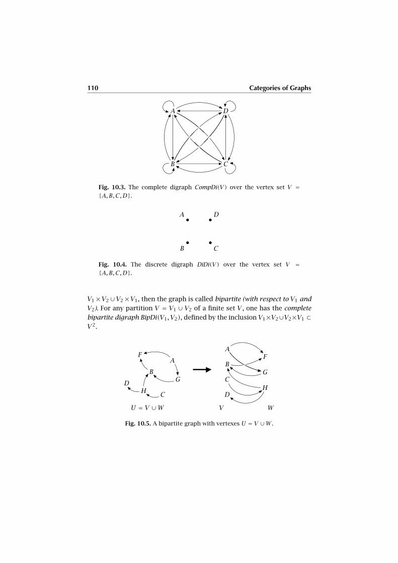
110 Categories of Graphs
DA
B C
Fig. 10.3. The complete digraph CompDi(V) over the vertex set V ={A,B,C,D}.
DA
B C
Fig. 10.4. The discrete digraph DiDi(V) over the vertex set V ={A,B,C,D}.
V1×V2∪V2×V1, then the graph is called bipartite (with respect to V1 and
V2). For any partition V = V1 ∪ V2 of a finite set V , one has the complete
bipartite digraph BipDi(V1, V2), defined by the inclusion V1×V2∪V2×V1 ⊂V2.
U = V ∪W
B
A
G
F
HD
C
V W
D
C
B
AF
G
H
Fig. 10.5. A bipartite graph with vertexes U = V ∪W .
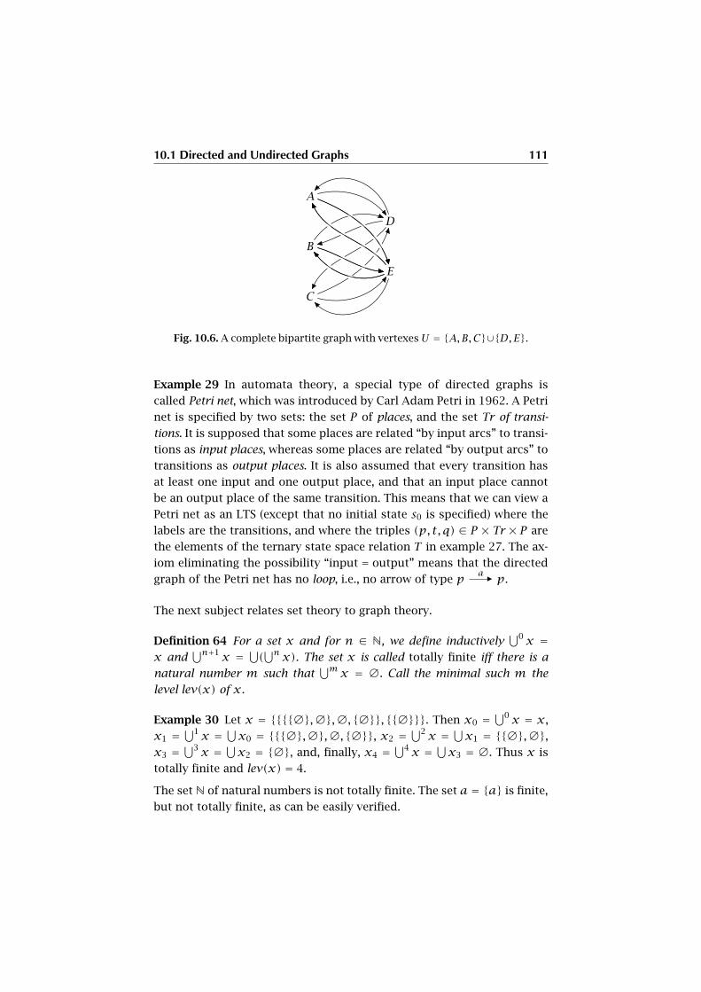
10.1 Directed and Undirected Graphs 111
C
B
A
E
D
Fig. 10.6. A complete bipartite graph with vertexes U = {A,B,C}∪{D,E}.
Example 29 In automata theory, a special type of directed graphs is
called Petri net, which was introduced by Carl Adam Petri in 1962. A Petri
net is specified by two sets: the set P of places, and the set Tr of transi-
tions. It is supposed that some places are related “by input arcs” to transi-
tions as input places, whereas some places are related “by output arcs” to
transitions as output places. It is also assumed that every transition has
at least one input and one output place, and that an input place cannot
be an output place of the same transition. This means that we can view a
Petri net as an LTS (except that no initial state s0 is specified) where the
labels are the transitions, and where the triples (p, t, q) ∈ P × Tr × P are
the elements of the ternary state space relation T in example 27. The ax-
iom eliminating the possibility “input = output” means that the directed
graph of the Petri net has no loop, i.e., no arrow of type pañ p.
The next subject relates set theory to graph theory.
Definition 64 For a set x and for n ∈ N, we define inductively⋃0x =
x and⋃n+1
x = ⋃(⋃nx). The set x is called totally finite iff there is a
natural number m such that⋃m
x = ∅. Call the minimal such m the
level lev(x) of x.
Example 30 Let x = {{{{∅},∅},∅, {∅}}, {{∅}}}. Then x0 =⋃0x = x,
x1 =⋃1x = ⋃
x0 = {{{∅},∅},∅, {∅}}, x2 =⋃2x = ⋃
x1 = {{∅},∅},x3 =
⋃3x = ⋃x2 = {∅}, and, finally, x4 =
⋃4x = ⋃x3 = ∅. Thus x is
totally finite and lev(x) = 4.
The set N of natural numbers is not totally finite. The set a = {a} is finite,
but not totally finite, as can be easily verified.
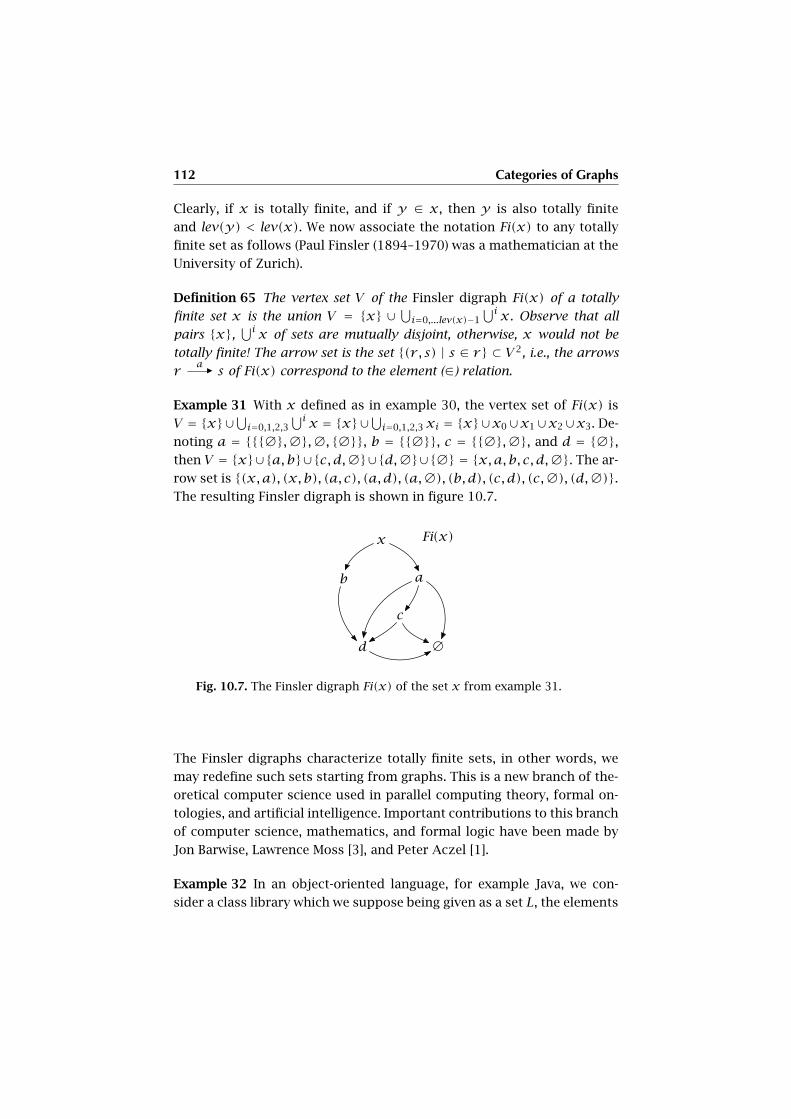
112 Categories of Graphs
Clearly, if x is totally finite, and if y ∈ x, then y is also totally finite
and lev(y) < lev(x). We now associate the notation Fi(x) to any totally
finite set as follows (Paul Finsler (1894–1970) was a mathematician at the
University of Zurich).
Definition 65 The vertex set V of the Finsler digraph Fi(x) of a totally
finite set x is the union V = {x} ∪ ⋃i=0,...lev(x)−1⋃ix. Observe that all
pairs {x}, ⋃i x of sets are mutually disjoint, otherwise, x would not be
totally finite! The arrow set is the set {(r , s) | s ∈ r} ⊂ V 2, i.e., the arrows
rañ s of Fi(x) correspond to the element (∈) relation.
Example 31 With x defined as in example 30, the vertex set of Fi(x) is
V = {x}∪⋃i=0,1,2,3⋃ix = {x}∪⋃i=0,1,2,3 xi = {x}∪x0∪x1∪x2∪x3. De-
noting a = {{{∅},∅},∅, {∅}}, b = {{∅}}, c = {{∅},∅}, and d = {∅},then V = {x}∪{a,b}∪{c, d,∅}∪{d,∅}∪{∅} = {x,a, b, c, d,∅}. The ar-
row set is {(x,a), (x, b), (a, c), (a,d), (a,∅), (b, d), (c, d), (c,∅), (d,∅)}.The resulting Finsler digraph is shown in figure 10.7.
x
b a
c
d ∅
Fi(x)
Fig. 10.7. The Finsler digraph Fi(x) of the set x from example 31.
The Finsler digraphs characterize totally finite sets, in other words, we
may redefine such sets starting from graphs. This is a new branch of the-
oretical computer science used in parallel computing theory, formal on-
tologies, and artificial intelligence. Important contributions to this branch
of computer science, mathematics, and formal logic have been made by
Jon Barwise, Lawrence Moss [3], and Peter Aczel [1].
Example 32 In an object-oriented language, for example Java, we con-
sider a class library which we suppose being given as a set L, the elements

10.1 Directed and Undirected Graphs 113
C of which represent the library’s classes, including (for simplicity) the
primitive type classes of integers, floating point numbers, strings, and
booleans. For each class C we have a number of fields (instance vari-
ables) defined by their names F and class types T ∈ L. This defines a
digraph ΛL, the vertex set being L, and the arrows being either the triples
(C, F, T) where F is the name of a field of class C, and where T is the type
class of F , or the pairs (C, S), where S is the direct superclass of C; we
set headΛ(C, F, T) = T and tailΛ(C, F, T) = C, or, for superclass arrows,
headΛ(C, S) = S and tailΛ(C, S) = C.
If one forgets about the direction in a digraph, the remaining structure
is that of an “undirected” graph, or simply “graph”. We shall henceforth
always write digraph for a directed graph, and graph for an undirected
graph, if confusion is unlikely.
Definition 66 An undirected graph (or simply graph) is a map Γ : A → 2V
between finite sets. The elements of the set A are called edges, the elements
of V are called vertexes of the graph. For a ∈ A and Γ(a) = {x,y}, we
also write xay , which is the same as y
ax.
The two-dimensional notation for graphs is similar to that of digraphs,
except that arrow heads are omitted.
Example 33 For each directed graph Γ , one generates the associated
graph |Γ | = |?| ◦ Γ , and for any given (undirected) graph Γ , one generates
an associated directed graph-→Γ = -→
? ◦ Γ , the latter construction supposing
that a section-→? for the graph’s vertex set is given.
F B
C D
|a||g|
|b||c| |d|
|e|
|Γ |
Fig. 10.8. The graph |Γ | associated to the graph from example 24 (fig-
ure 10.1).
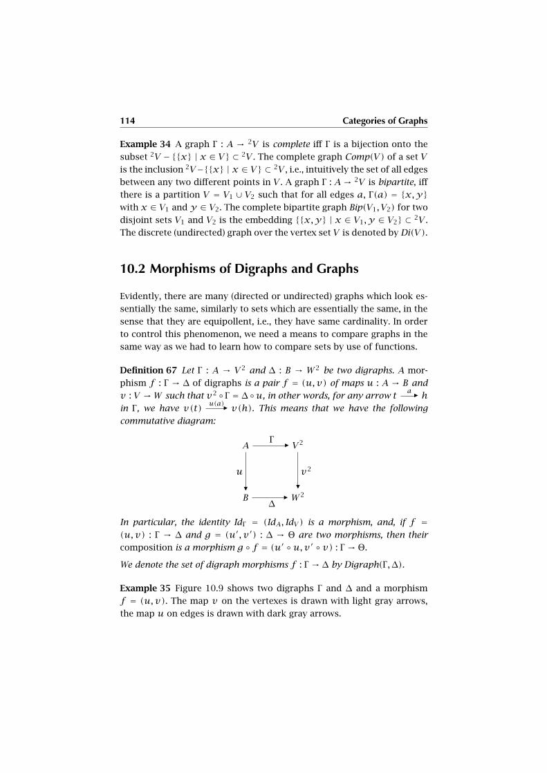
114 Categories of Graphs
Example 34 A graph Γ : A → 2V is complete iff Γ is a bijection onto the
subset 2V −{{x} | x ∈ V} ⊂ 2V . The complete graph Comp(V) of a set V
is the inclusion 2V−{{x} | x ∈ V} ⊂ 2V , i.e., intuitively the set of all edges
between any two different points in V . A graph Γ : A → 2V is bipartite, iff
there is a partition V = V1 ∪ V2 such that for all edges a, Γ(a) = {x,y}with x ∈ V1 and y ∈ V2. The complete bipartite graph Bip(V1, V2) for two
disjoint sets V1 and V2 is the embedding {{x,y} | x ∈ V1, y ∈ V2} ⊂ 2V .
The discrete (undirected) graph over the vertex set V is denoted by Di(V).
10.2 Morphisms of Digraphs and Graphs
Evidently, there are many (directed or undirected) graphs which look es-
sentially the same, similarly to sets which are essentially the same, in the
sense that they are equipollent, i.e., they have same cardinality. In order
to control this phenomenon, we need a means to compare graphs in the
same way as we had to learn how to compare sets by use of functions.
Definition 67 Let Γ : A → V 2 and ∆ : B → W 2 be two digraphs. A mor-
phism f : Γ → ∆ of digraphs is a pair f = (u,v) of maps u : A → B and
v : V → W such that v2 ◦ Γ = ∆◦u, in other words, for any arrow tañ h
in Γ , we have v(t)u(a)
ñ v(h). This means that we have the following
commutative diagram:
AΓ
ñ V2
B
u
�
Ɩ W 2
v2
�
In particular, the identity IdΓ = (IdA, IdV ) is a morphism, and, if f =(u,v) : Γ → ∆ and g = (u′, v′) : ∆ → Θ are two morphisms, then their
composition is a morphism g ◦ f = (u′ ◦u,v′ ◦ v) : Γ → Θ.
We denote the set of digraph morphisms f : Γ → ∆ by Digraph(Γ ,∆).
Example 35 Figure 10.9 shows two digraphs Γ and ∆ and a morphism
f = (u,v). The map v on the vertexes is drawn with light gray arrows,
the map u on edges is drawn with dark gray arrows.
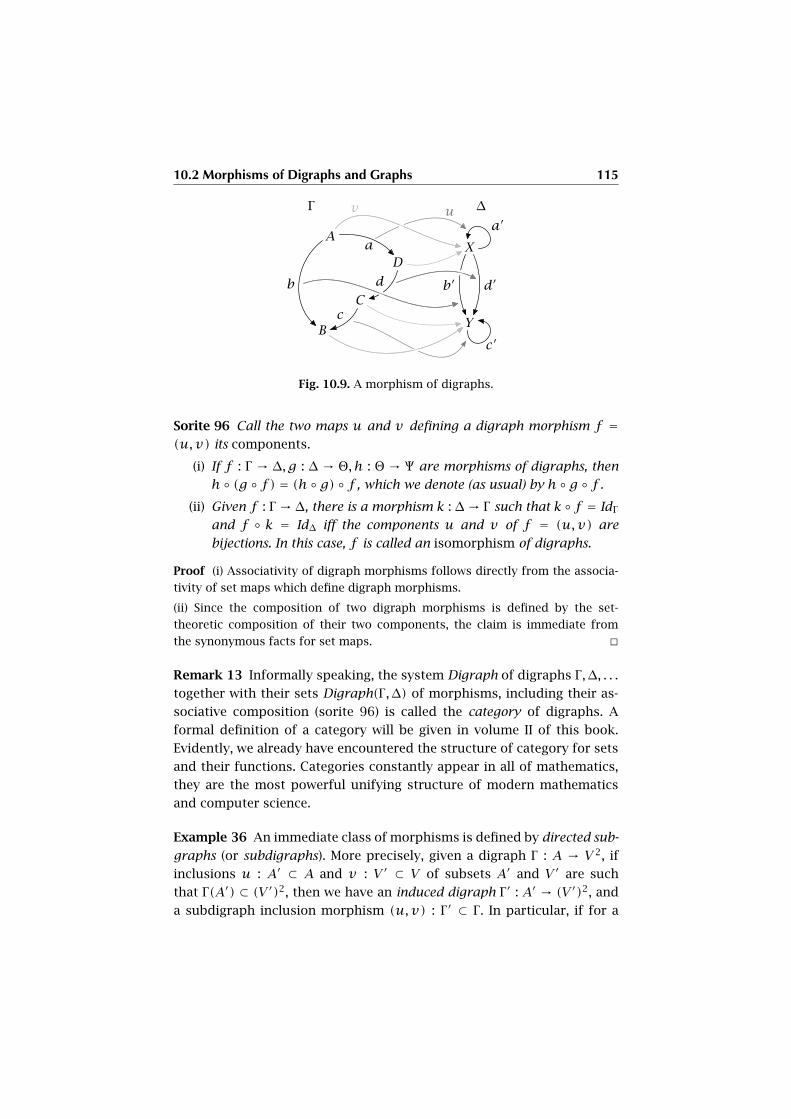
10.2 Morphisms of Digraphs and Graphs 115
A
B
D
C
X
Y
a′
c′
a
d
c
b b′ d′
v uΓ ∆
Fig. 10.9. A morphism of digraphs.
Sorite 96 Call the two maps u and v defining a digraph morphism f =(u,v) its components.
(i) If f : Γ → ∆, g : ∆ → Θ, h : Θ → Ψ are morphisms of digraphs, then
h ◦ (g ◦ f) = (h ◦ g) ◦ f , which we denote (as usual) by h ◦ g ◦ f .
(ii) Given f : Γ → ∆, there is a morphism k : ∆→ Γ such that k ◦ f = IdΓ
and f ◦ k = Id∆ iff the components u and v of f = (u,v) are
bijections. In this case, f is called an isomorphism of digraphs.
Proof (i) Associativity of digraph morphisms follows directly from the associa-
tivity of set maps which define digraph morphisms.
(ii) Since the composition of two digraph morphisms is defined by the set-
theoretic composition of their two components, the claim is immediate from
the synonymous facts for set maps. �
Remark 13 Informally speaking, the system Digraph of digraphs Γ ,∆, . . .
together with their sets Digraph(Γ ,∆) of morphisms, including their as-
sociative composition (sorite 96) is called the category of digraphs. A
formal definition of a category will be given in volume II of this book.
Evidently, we already have encountered the structure of category for sets
and their functions. Categories constantly appear in all of mathematics,
they are the most powerful unifying structure of modern mathematics
and computer science.
Example 36 An immediate class of morphisms is defined by directed sub-
graphs (or subdigraphs). More precisely, given a digraph Γ : A → V 2, if
inclusions u : A′ ⊂ A and v : V ′ ⊂ V of subsets A′ and V ′ are such
that Γ(A′) ⊂ (V ′)2, then we have an induced digraph Γ ′ : A′ → (V ′)2, and
a subdigraph inclusion morphism (u,v) : Γ ′ ⊂ Γ . In particular, if for a
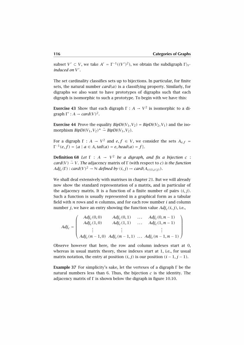
116 Categories of Graphs
subset V ′ ⊂ V , we take A′ = Γ−1((V ′)2), we obtain the subdigraph Γ |V ′induced on V ′.
The set cardinality classifies sets up to bijections. In particular, for finite
sets, the natural number card(a) is a classifying property. Similarly, for
digraphs we also want to have prototypes of digraphs such that each
digraph is isomorphic to such a prototype. To begin with we have this:
Exercise 43 Show that each digraph Γ : A → V 2 is isomorphic to a di-
graph Γ ′ : A→ card(V)2.
Exercise 44 Prove the equality BipDi(V1, V2) = BipDi(V2, V1) and the iso-
morphism BipDi(V1, V2)∗ ∼→ BipDi(V1, V2).
For a digraph Γ : A → V 2 and e, f ∈ V , we consider the sets Ae,f =Γ−1(e, f ) = {a | a ∈ A, tail(a) = e,head(a) = f}.
Definition 68 Let Γ : A → V 2 be a digraph, and fix a bijection c :
card(V)∼→ V . The adjacency matrix of Γ (with respect to c) is the function
Adjc(Γ) : card(V)2 → N defined by (i, j), card(Ac(i),c(j)).
We shall deal extensively with matrixes in chapter 21. But we will already
now show the standard representation of a matrix, and in particular of
the adjacency matrix. It is a function of a finite number of pairs (i, j).
Such a function is usually represented in a graphical form as a tabular
field with n rows and n columns, and for each row number i and column
number j, we have an entry showing the function value Adjc(i, j), i.e.,
Adjc =
Adjc(0,0) Adjc(0,1) . . . Adjc(0, n− 1)
Adjc(1,0) Adjc(1,1) . . . Adjc(1, n− 1)...
......
Adjc(n− 1,0) Adjc(n− 1,1) . . . Adjc(n− 1, n− 1)
Observe however that here, the row and column indexes start at 0,
whereas in usual matrix theory, these indexes start at 1, i.e., for usual
matrix notation, the entry at position (i, j) is our position (i− 1, j − 1).
Example 37 For simplicity’s sake, let the vertexes of a digraph Γ be the
natural numbers less than 6. Thus, the bijection c is the identity. The
adjacency matrix of Γ is shown below the digraph in figure 10.10.

10.2 Morphisms of Digraphs and Graphs 117
0
1
4
2
35
Γ
Adjc(Γ) =
0 0 0 0 0 0
1 0 1 0 2 0
0 0 0 0 0 2
0 0 0 1 0 0
0 0 0 0 0 0
2 0 0 0 0 1
Fig. 10.10. Adjacency matrix of a digraph.
The following numerical criterion for isomorphic digraphs is very impor-
tant for the computerized representations of digraphs:
Proposition 97 If Γ and ∆ are two digraphs such that Adj(Γ) = Adj(∆),
then they are isomorphic, i.e., there is an isomorphism Γ∼→ ∆.
Proof Suppose that for two digraphs Γ : A → V 2 and ∆ : B → W 2, Adj(Γ) =Adj(∆). Then the number of rows of the two matrixes is the same, and therefore
we have a bijection v : V → W such that the matrix index (i, j) in Adj(Γ) corre-
sponds to the same index of Adj(∆). Moreover, we have A = ⊔x∈V2 Γ
−1(x) and
B = ⊔y∈W2 ∆
−1(y). But since by hypothesis card(Γ−1(x)) = card(∆−1(v2(x))
for all x ∈ V , setting v2 = v × v , we have bijections ux : Γ−1(x) → ∆−1(v2(x))
and their disjoint union yields a bijection u : A → B which defines the desired
isomorphism (u,v). �
So the adjacency matrix of a digraph describes the digraph “up to iso-
morphisms”. The converse is not true, but it can easily be said what is
missing: Essentially, we have to take into account the bijection c, which
labels the vertexes. In fact, if Γ∼→ ∆, then their adjacency matrixes are re-
lated to each other by conjugation with a permutation matrix relabeling
the vertexes.
Example 38 The bipartite digraphs can now be denoted by simple num-
bers, i.e., if n and m are natural numbers, we have the bipartite digraph
BipDi(n,m), and every bipartite digraph BipDi(V1, V2) with card(V1) = n
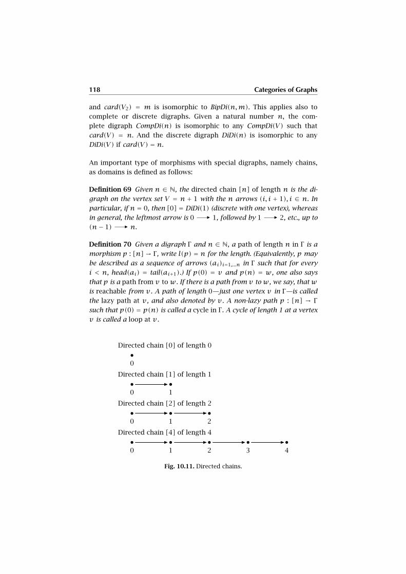
118 Categories of Graphs
and card(V2) = m is isomorphic to BipDi(n,m). This applies also to
complete or discrete digraphs. Given a natural number n, the com-
plete digraph CompDi(n) is isomorphic to any CompDi(V) such that
card(V) = n. And the discrete digraph DiDi(n) is isomorphic to any
DiDi(V) if card(V) = n.
An important type of morphisms with special digraphs, namely chains,
as domains is defined as follows:
Definition 69 Given n ∈ N, the directed chain [n] of length n is the di-
graph on the vertex set V = n + 1 with the n arrows (i, i + 1), i ∈ n. In
particular, if n = 0, then [0] = DiDi(1) (discrete with one vertex), whereas
in general, the leftmost arrow is 0 ñ 1, followed by 1 ñ 2, etc., up to
(n− 1) ñ n.
Definition 70 Given a digraph Γ and n ∈ N, a path of length n in Γ is a
morphism p : [n]→ Γ , write l(p) = n for the length. (Equivalently, p may
be described as a sequence of arrows (ai)i=1,...n in Γ such that for every
i < n, head(ai) = tail(ai+1).) If p(0) = v and p(n) = w, one also says
that p is a path from v tow. If there is a path from v tow, we say, thatw
is reachable from v . A path of length 0—just one vertex v in Γ—is called
the lazy path at v , and also denoted by v . A non-lazy path p : [n] → Γ
such that p(0) = p(n) is called a cycle in Γ . A cycle of length 1 at a vertex
v is called a loop at v .
0
Directed chain [0] of length 0
0 1
Directed chain [1] of length 1
0 1 2
Directed chain [2] of length 2
0 1 2 3 4
Directed chain [4] of length 4
Fig. 10.11. Directed chains.
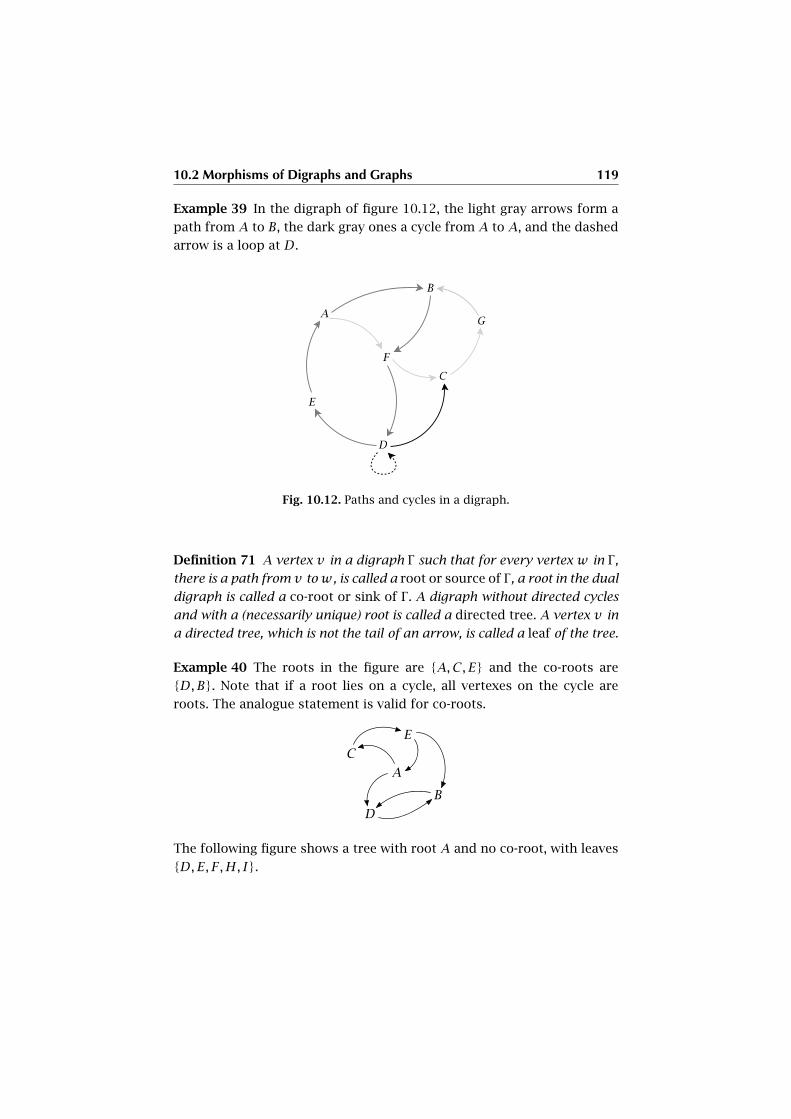
10.2 Morphisms of Digraphs and Graphs 119
Example 39 In the digraph of figure 10.12, the light gray arrows form a
path from A to B, the dark gray ones a cycle from A to A, and the dashed
arrow is a loop at D.
Fig. 10.12. Paths and cycles in a digraph.
Definition 71 A vertex v in a digraph Γ such that for every vertex w in Γ ,
there is a path from v tow, is called a root or source of Γ , a root in the dual
digraph is called a co-root or sink of Γ . A digraph without directed cycles
and with a (necessarily unique) root is called a directed tree. A vertex v in
a directed tree, which is not the tail of an arrow, is called a leaf of the tree.
Example 40 The roots in the figure are {A,C, E} and the co-roots are
{D,B}. Note that if a root lies on a cycle, all vertexes on the cycle are
roots. The analogue statement is valid for co-roots.
A
B
C
D
E
The following figure shows a tree with root A and no co-root, with leaves
{D,E, F,H, I}.

120 Categories of Graphs
A
B C
D E F G
H I
Exercise 45 Given two paths p and q of lengths n and m, respectively,
in a digraph Γ such that p ends where q begins, we have an evident com-
position qp of paths of length l(qp) = n +m = l(q) + l(p), defined by
joining the two arrow sequences in the connecting vertex. Composition
of paths is associative, and the composition with a lazy path at v , if it is
defined, yields vp = p, or pv = p.
This allows us to characterize totally finite sets by their Finsler digraphs
(see definition 65). To this end, we consider the following subgraph con-
struction: If Γ is a graph and v a vertex, we define v〉 to be the set of
all vertexes w such that there is a path from v to w.The directed sub-
x
b a
c
d ∅
Fi(x)
Fig. 10.13. The vertexes and edges of the subdigraph a〉 of Fi(x) from
figure 10.7 are shown in bold.
graph induced on v〉 is also denoted by v〉 and is called the subdigraph
generated by v .
Proposition 98 A digraph Γ is isomorphic to a Finsler digraph Fi(x) of a
totally finite set x iff it is a directed tree such that for any two vertexes v1
and v2, if v1〉 is isomorphic to v2〉, then v1 = v2.
10.2 Morphisms of Digraphs and Graphs 121
Proof Let x be totally finite. Then in the Finsler digraph Fi(x), every y ∈ xis reached from the vertex x. And if z ∈ ⋃n+1
x = ⋃⋃nx, then it is reached
from a selected element in⋃nx. So x is the root of Fi(x). If y is a vertex in
Fi(x), then clearly y〉 = Fi(y). Let us show by induction on lev(y) that an iso-
morphism Fi(y)∼→ Fi(z) implies y = z. In fact, if lev(y) = 0, then Fi(y) and
Fi(z) are both one-point digraphs, and both y and z must be the empty set. In
general, if Fi(y)∼→ Fi(z), then the roots must also correspond under the given
isomorphism, and therefore there is a bijection between the vertexes yi reached
from y by an arrow, and the vertexes zi reached from z by an arrow. If zi cor-
responds to yi, then also zi〉 ∼→ yi〉, and therefore, by recursion, yi = zi, which
implies y = z. Conversely, if a directed tree F : V → A2 is such that any two
vertexes v1 and v2 with v1〉 ∼→ v2〉 must be equal, then it follows by induction
on the length of the maximal path from a given vertex that F is isomorphic to
the Finsler digraph of a totally finite set. In fact, if a directed tree has maximal
path length 0 from the root, it is the Finsler digraph of the empty set. In general,
the vertexes yi, i = 1, . . . k reached from the root y by an arrow have a shorter
maximal path than the root and are also directed trees with the supposed condi-
tions. So by recursion, they are Finsler digraphs Fi(ti) of totally finite, mutually
different sets ti. Then evidently, y is isomorphic to the Finsler digraph of the set
{ti | i = 1, . . . k}. �
We now turn to the subject of morphisms between undirected graphs. We
need the undirected variant of the square map v2 : V2 → W 2 associated
with a map v : V → W , i.e., 2v : 2V → 2W : {x,y}, {v(x), v(y)}.
Definition 72 Let Γ : A→ 2V and ∆ : B → 2W be two graphs. A morphism
f : Γ → ∆ of graphs is a pair f = (u,v) of maps u : A → B and v : V → Wsuch that 2v ◦ Γ = ∆ ◦ u, in other words, for any edge t
ah in Γ , we
have v(t)u(a)
v(h). This means we have the commutative diagram
AΓ
ñ 2V
B
u
�
Ɩ 2W
2v
�
In particular, the identity IdΓ = (IdA, IdV ) is a morphism, and, if f =(u,v) : Γ → ∆ and g = (u′, v′) : ∆ → Θ are two morphisms, then their
composition is a morphism g ◦ f = (u′ ◦u,v′ ◦ v) : Γ → Θ.
Exercise 46 Show that the mapping Γ , |Γ | can be extended to mor-
phisms, i.e., if f = (u,v) : Γ → ∆, is a morphism, then so is |f | : |Γ | → |∆|.Also, |IdΓ | = Id|Γ |, and |f ◦ g| = |f | ◦ |g|.
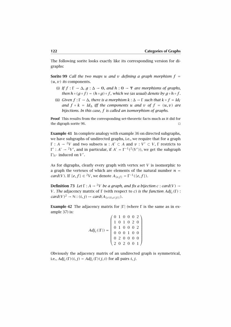
122 Categories of Graphs
The following sorite looks exactly like its corresponding version for di-
graphs:
Sorite 99 Call the two maps u and v defining a graph morphism f =(u,v) its components.
(i) If f : Γ → ∆, g : ∆ → Θ, and h : Θ → Ψ are morphisms of graphs,
then h◦(g ◦f) = (h◦g)◦f , which we (as usual) denote by g ◦h◦f .
(ii) Given f : Γ → ∆, there is a morphism k : ∆→ Γ such that k ◦ f = IdΓ
and f ◦ k = Id∆ iff the components u and v of f = (u,v) are
bijections. In this case, f is called an isomorphism of graphs.
Proof This results from the corresponding set-theoretic facts much as it did for
the digraph sorite 96. �
Example 41 In complete analogy with example 36 on directed subgraphs,
we have subgraphs of undirected graphs, i.e., we require that for a graph
Γ : A → 2V and two subsets u : A′ ⊂ A and v : V ′ ⊂ V , Γ restricts to
Γ ′ : A′ → 2V ′, and in particular, if A′ = Γ−1(2(V ′)), we get the subgraph
Γ |V ′ induced on V ′.
As for digraphs, clearly every graph with vertex set V is isomorphic to
a graph the vertexes of which are elements of the natural number n =card(V). If {e, f} ∈ 2V , we denote A{e,f} = Γ−1({e, f}).
Definition 73 Let Γ : A→ 2V be a graph, and fix a bijection c : card(V)→V . The adjacency matrix of Γ (with respect to c) is the function Adjc(Γ) :
card(V)2 → N : (i, j), card(A{c(i),c(j)}).
Example 42 The adjacency matrix for |Γ | (where Γ is the same as in ex-
ample 37) is:
Adjc(|Γ |) =
0 1 0 0 0 2
1 0 1 0 2 0
0 1 0 0 0 2
0 0 0 1 0 0
0 2 0 0 0 0
2 0 2 0 0 1
Obviously the adjacency matrix of an undirected graph is symmetrical,
i.e., Adjc(Γ)(i, j) = Adjc(Γ)(j, i) for all pairs i, j.

10.2 Morphisms of Digraphs and Graphs 123
Proposition 100 If Γ and ∆ are two graphs such that Adj(Γ) = Adj(∆),
then they are isomorphic.
Proof The proof of this proposition is completely analogous to the proof of the
corresponding proposition 97 for digraphs. �
Definition 74 Given n ∈ N, the chain |n| of length n is the graph on the
vertex set V = n + 1 such that we have the n edges {i, i + 1}, i ∈ n. In
particular, if n = 0, then |0| = Di(1) (discrete with one vertex), whereas
in general, the leftmost edge is 0 1, followed by 1 2, etc., up to
(n− 1) n.
Example 43 For any natural number n, we have the complete graph
Comp(n), which in literature is often denoted by Kn, it is isomorphic
to any complete graph Comp(V) with card(V) = n. For two natural num-
bers n and m, we have the complete bipartite graph Bip(n,m), often
denoted by Kn,m, which is isomorphic to any complete bipartite graph
Bip(V1, V2) such that card(V1) = n and card(V2) =m.
K1 K2 K3 K4 K5
Fig. 10.14. The complete graphs Kn for n = 1 . . .5.
Definition 75 Given a graph Γ and n ∈ N, a walk of length n in Γ is a
morphism p : |n| → Γ , we write l(p) = n for its length. If p(0) = v and
p(n) = w, one also says that p is a walk from v to w. If there is a walk
from v to w, we say that w is reachable from v . A walk of length 0 (just
one vertex v in Γ ) is called the lazy walk at v , and also denoted by v . A
non-lazy walk p : |n| → Γ such that p(0) = p(n) is called a cycle in Γ . A
cycle of length 1 at a vertex v is called a loop at v .
A graph is said to be connected if any two vertexes can be joined by a
walk. A connected graph without (undirected) cycles is called a tree.
A directed graph Γ is called connected if |Γ | is so.
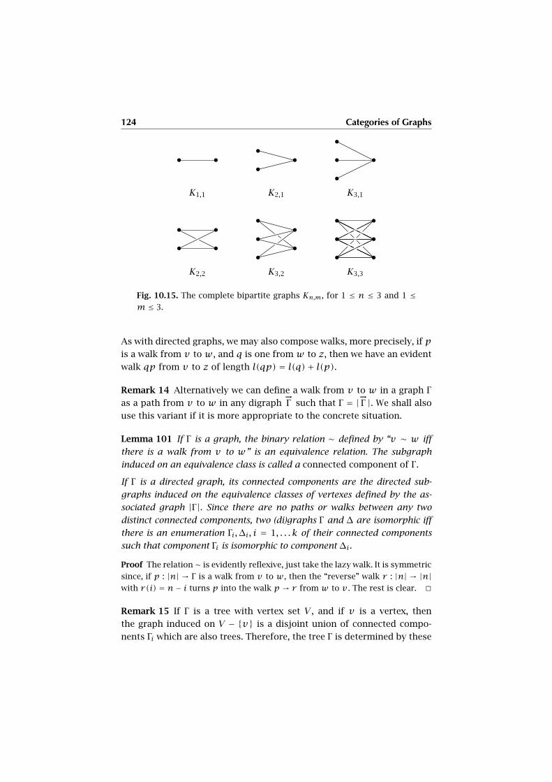
124 Categories of Graphs
K1,1 K2,1 K3,1
K2,2 K3,2 K3,3
Fig. 10.15. The complete bipartite graphs Kn,m, for 1 ≤ n ≤ 3 and 1 ≤m ≤ 3.
As with directed graphs, we may also compose walks, more precisely, if p
is a walk from v to w, and q is one from w to z, then we have an evident
walk qp from v to z of length l(qp) = l(q)+ l(p).
Remark 14 Alternatively we can define a walk from v to w in a graph Γ
as a path from v to w in any digraph-→Γ such that Γ = | -→Γ |. We shall also
use this variant if it is more appropriate to the concrete situation.
Lemma 101 If Γ is a graph, the binary relation ∼ defined by “v ∼ w iff
there is a walk from v to w” is an equivalence relation. The subgraph
induced on an equivalence class is called a connected component of Γ .
If Γ is a directed graph, its connected components are the directed sub-
graphs induced on the equivalence classes of vertexes defined by the as-
sociated graph |Γ |. Since there are no paths or walks between any two
distinct connected components, two (di)graphs Γ and ∆ are isomorphic iff
there is an enumeration Γi,∆i, i = 1, . . . k of their connected components
such that component Γi is isomorphic to component ∆i.
Proof The relation∼ is evidently reflexive, just take the lazy walk. It is symmetric
since, if p : |n| → Γ is a walk from v to w, then the “reverse” walk r : |n| → |n|with r(i) = n− i turns p into the walk p → r from w to v . The rest is clear. �
Remark 15 If Γ is a tree with vertex set V , and if v is a vertex, then
the graph induced on V − {v} is a disjoint union of connected compo-
nents Γi which are also trees. Therefore, the tree Γ is determined by these

10.3 Cycles 125
subtrees Γi, together with the vertexes being joined by an edge from v
to determined vertexes vi in Γi (in fact, if there were more than one such
vertex, we would have cycles, and Γ would not be a tree). This allows us to
define the tree concept recursively by the total vertex set V , the selected
vertex v , the edges v vi, and the subtrees Γi. This is the definition of
a tree given by Donald Knuth in his famous book, “The Art of Computer
Programming” [31]. It has however the shortcoming that it distinguishes
a vertex v , which is not the intrinsic property of a tree. For computer
science it has the advantage that it is constructive and recursive.
10.3 Cycles
In this section, we want to state a number of elementary facts concerning
the existence or absence of cycles in directed and undirected graphs.
Definition 76 An Euler cycle e in a digraph/graph Γ is a cycle such that
every vertex and every arrow/edge of Γ lies on the cycle (i.e., e is surjective
on the vertexes and on the arrows/edges), but every arrow/edge appears
only once (i.e., e is bijective on the arrows/edges).
A Hamilton cycle h in a digraph/graph Γ is a cycle which contains ev-
ery vertex exactly (i.e., h is surjective on the vertexes), except for the
start and end vertex which it its twice (i.e., is a bijection on the vertexes
0,1,2, . . . l(h)− 1).
The condition for the existence of Euler cycles in digraphs uses the degree
of a vertex:
Definition 77 If v is a vertex of a digraph Γ : A → V 2, the head degree of
v is the number
deg−(v) = card({h | h ∈ A,head(h) = v}),
the tail degree of v is the number
deg+(v) = card({h | h ∈ A, tail(h) = v}),
and the degree of v is the number
deg(v) = deg−(v)+ deg+(v).

126 Categories of Graphs
For a graph Γ , the degree deg(v) of a vertex v is defined as the degree of
v in any of the digraphs-→Γ such that | -→Γ | = Γ ; observe that this number is
independent of the choice of the digraph-→Γ .
Here are two classical results by Leonhard Euler (1707–1783):
Proposition 102 Let Γ be a digraph. Then it has an Euler cycle iff it is
connected and for every vertex v , we have deg−(v) = deg+(v).
Proof In both implications we may give the proof for the subgraph of Γ obtained
by omitting the loops. We may then put the loops back again without changing
the validity of the proof.
If Γ has an Euler cycle c : [n] → Γ , any two vertexes are connected by a sub-
path associated to this cycle, so Γ is connected. If v is a vertex of Γ , and if
wañ v,w ≠ v is an arrow of Γ , then a appears right before a subsequent
arrow va′ñ w′ in the cycle c. But these two arrows appear exactly once each
in c, and therefore deg−(v) = deg
+(v).
Conversely, if Γ is connected and for every vertex v , deg−(v) = deg
+(v), then
we first construct a covering of Γ by cycles ci. Here we need only the hypothesis
that the degrees are all even. Let a be an arrow of Γ , then there must exist an
arrow a′ starting from head(a). The head of a′ must also have an arrow a′′ the
tail of which is the head of a′. After a finite number of such steps, we end up at
a vertex which we had already encountered before, and this defines a first cycle.
Now omit all these cycle’s arrows, and the hypothesis about the even number
of degrees still holds, but for the smaller digraph obtained after elimination of
the cycle’s arrows. By induction we have a covering of this digraph by cycles,
and, together with our first cycle obtain the desired covering. Clearly, a union of
cycles with disjoint arrows covering a connected digraph is again a cycle. To see
this observe that (1) a cycle may start at any of its vertexes; (2) if two cycles c
and d in Γ have the vertex v in common, but have disjoint arrow sets, then there
is also a cycle containing the union of these arrow sets; (3) if Γ is connected,
any given cycle in Γ can be extended by adding to it another cycle of the given
covering, having disjoint arrows. �
Proposition 103 Let Γ be a graph. Then it has an Euler cycle iff it is con-
nected and for every vertex v , deg(v) is an even number (a multiple of
2).
Proof The proof is similar to the case of digraphs, except that the existence
of an Euler cycle for an even number deg(v) in each vertex v has to shown.
Here, we may couple edges at v in pairs of edges and associate with each pair
one incoming and one outgoing arrow. This procedure yields a digraph over the
given graph, and we may apply proposition 102. �
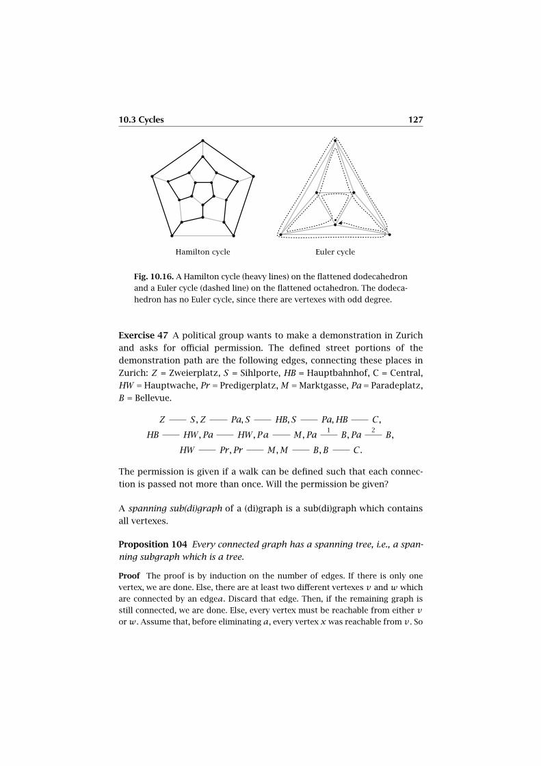
10.3 Cycles 127
Fig. 10.16. A Hamilton cycle (heavy lines) on the flattened dodecahedron
and a Euler cycle (dashed line) on the flattened octahedron. The dodeca-
hedron has no Euler cycle, since there are vertexes with odd degree.
Exercise 47 A political group wants to make a demonstration in Zurich
and asks for official permission. The defined street portions of the
demonstration path are the following edges, connecting these places in
Zurich: Z = Zweierplatz, S = Sihlporte, HB = Hauptbahnhof, C = Central,
HW = Hauptwache, Pr = Predigerplatz,M = Marktgasse, Pa = Paradeplatz,
B = Bellevue.
Z S,Z Pa, S HB, S Pa,HB C,
HB HW ,Pa HW , Pa M,Pa1B,Pa
2B,
HW Pr,Pr M,M B,B C.
The permission is given if a walk can be defined such that each connec-
tion is passed not more than once. Will the permission be given?
A spanning sub(di)graph of a (di)graph is a sub(di)graph which contains
all vertexes.
Proposition 104 Every connected graph has a spanning tree, i.e., a span-
ning subgraph which is a tree.
Proof The proof is by induction on the number of edges. If there is only one
vertex, we are done. Else, there are at least two different vertexes v and w which
are connected by an edgea. Discard that edge. Then, if the remaining graph is
still connected, we are done. Else, every vertex must be reachable from either v
orw. Assume that, before eliminating a, every vertex x was reachable from v . So

128 Categories of Graphs
if x is still reachable from v it pertains to the connected component of v , else,
there walk from x to v must traverse w via a. But then, x is in the connected
component of w. So the graph without a has exactly the two connected compo-
nents Cv of v and Cw ofw. By induction, each component Cv , Cw has a spanning
tree Tv , Tw , respectively. Adding the edge a to the union of the disjoint spanning
trees Tv and Tw still yields a tree, which is the required spanning tree. �
Fig. 10.17. Spanning tree of an undirected graph.

CHAPTER 11
Construction of Graphs
We already know about some constructions of new (di)graphs from given
ones: The dual digraph is such a construction. The spanning tree is a
second one. Here more of these constructions are presented.
We have seen in set theory that there are universal constructions of new
sets from given ones, such as the Cartesian product a × b, the coprod-
uct a t b, and the function set ab. In graph theory, one also has such
constructions which we discuss now. They are of very practical use, espe-
cially in computer science where the systematic construction of objects
is a core business of software engineering.
Given two digraphs Γ : A → V 2 and ∆ : B → W 2, we have the Cartesian
product Γ ×∆ : A×B → (V ×W)2, defined by the canonical1 isomorphism
of sets t : V 2 ×W 2 → (V ×W)2 : ((e1, e2), (f1, f2)), ((e1, f1), (e2, f2)). In
other words, we have
head(a, b) = (head(a),head(b))
tail(a, b) = (tail(a), tail(b)).
Example 44 Figure 11.1 shows the Cartesian product of two digraphs Γ
and ∆.
1 In mathematics, a construction is called “canonical” if no particular trick is
necessary for its elaboration, it is realized by the given “surface structures”.
Attention: the attribute “natural”, which we would also like to use instead, is
reserved for a technical term in category theory.
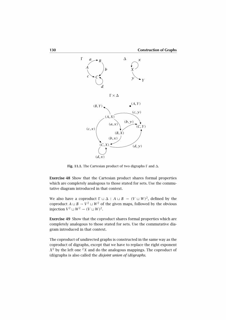
130 Construction of Graphs
Γ
A
B
Cc
a
b
d
∆
X
Yy
x
Γ ×∆
(B, Y)(A, Y)
(A,X)
(B,X)
(C,X)
(C, Y)
(d,x)
(c,x)
(a,x)
(b,x)
(b,y)
(d,y)
(c,y)
Fig. 11.1. The Cartesian product of two digraphs Γ and ∆.
Exercise 48 Show that the Cartesian product shares formal properties
which are completely analogous to those stated for sets. Use the commu-
tative diagram introduced in that context.
We also have a coproduct Γ t ∆ : A t B → (V t W)2, defined by the
coproduct A t B → V 2 tW 2 of the given maps, followed by the obvious
injection V 2 tW 2 → (V tW)2.
Exercise 49 Show that the coproduct shares formal properties which are
completely analogous to those stated for sets. Use the commutative dia-
gram introduced in that context.
The coproduct of undirected graphs is constructed in the same way as the
coproduct of digraphs, except that we have to replace the right exponent
X2 by the left one 2X and do the analogous mappings. The coproduct of
(di)graphs is also called the disjoint union of (di)graphs.
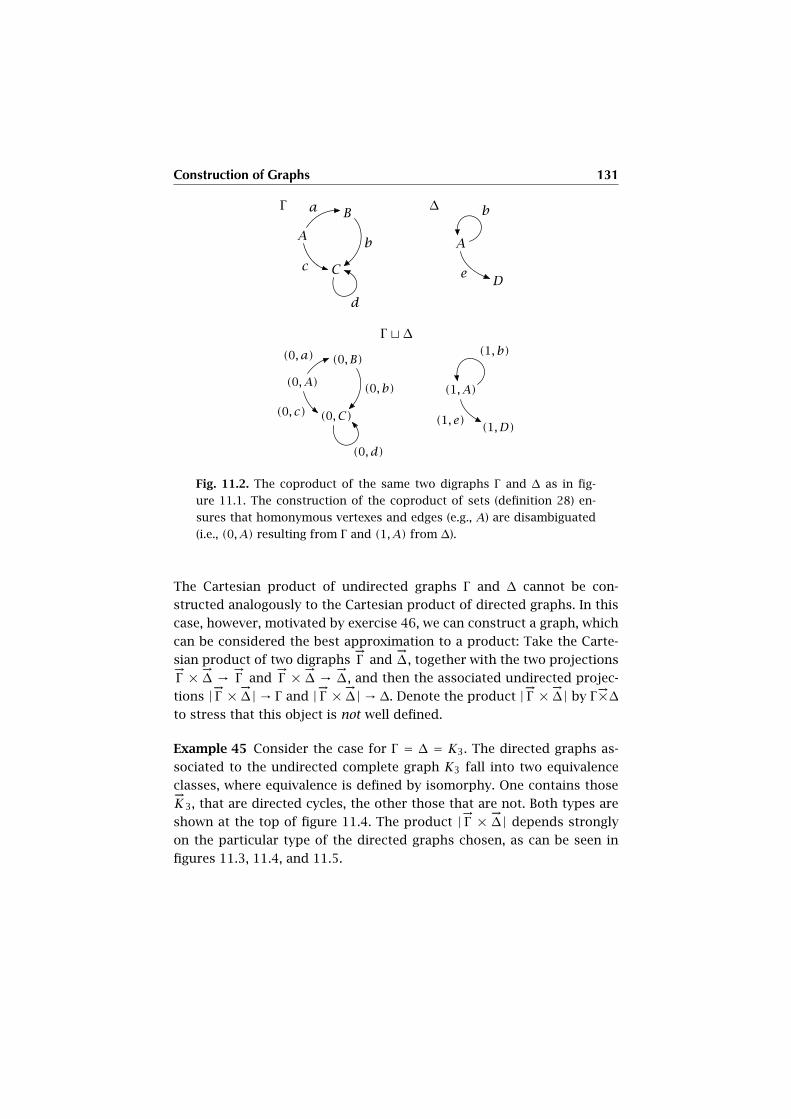
Construction of Graphs 131
Γ
A
B
Cc
a
b
d
∆
A
De
b
Γ t∆
(0, A)
(0, B)
(0, C)(0, c)
(0, a)
(0, b)
(0, d)
(1, A)
(1,D)(1, e)
(1, b)
Fig. 11.2. The coproduct of the same two digraphs Γ and ∆ as in fig-
ure 11.1. The construction of the coproduct of sets (definition 28) en-
sures that homonymous vertexes and edges (e.g., A) are disambiguated
(i.e., (0, A) resulting from Γ and (1, A) from ∆).
The Cartesian product of undirected graphs Γ and ∆ cannot be con-
structed analogously to the Cartesian product of directed graphs. In this
case, however, motivated by exercise 46, we can construct a graph, which
can be considered the best approximation to a product: Take the Carte-
sian product of two digraphs-→Γ and
-→∆ , together with the two projections
-→Γ × -→
∆ → -→Γ and
-→Γ × -→
∆ → -→∆ , and then the associated undirected projec-
tions | -→Γ × -→∆| → Γ and | -→Γ × -→
∆| → ∆. Denote the product | -→Γ × -→∆| by Γ
-→×∆to stress that this object is not well defined.
Example 45 Consider the case for Γ = ∆ = K3. The directed graphs as-
sociated to the undirected complete graph K3 fall into two equivalence
classes, where equivalence is defined by isomorphy. One contains those-→K3, that are directed cycles, the other those that are not. Both types are
shown at the top of figure 11.4. The product | -→Γ × -→∆| depends strongly
on the particular type of the directed graphs chosen, as can be seen in
figures 11.3, 11.4, and 11.5.
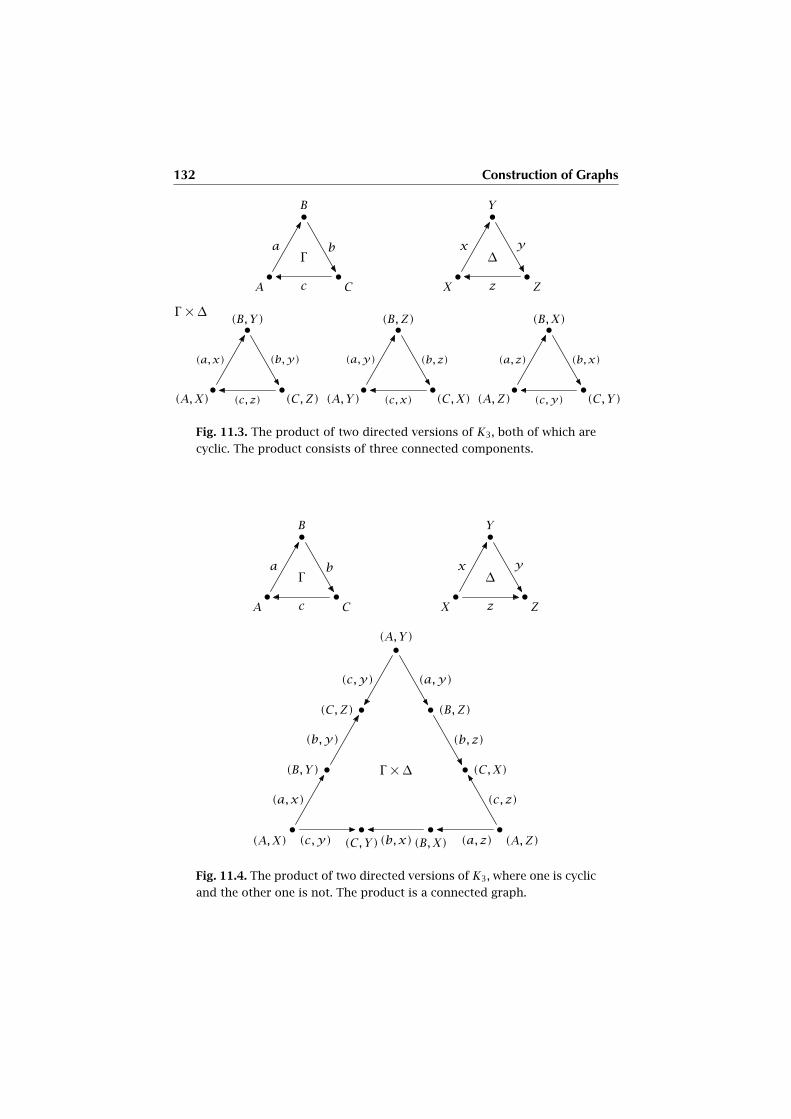
132 Construction of Graphs
B
CA
b
c
aΓ
Y
ZX
y
z
x∆
(B, Y)
(C,Z)(A,X)
(b,y)
(c, z)
(a,x)
(B, Z)
(C,X)(A,Y)
(b, z)
(c, x)
(a,y)
(B,X)
(C, Y)(A,Z)
(b,x)
(c,y)
(a, z)
Γ ×∆
Fig. 11.3. The product of two directed versions of K3, both of which are
cyclic. The product consists of three connected components.
B
CA
b
c
aΓ
Y
ZX
y
z
x∆
(A, Y)
(B, Z)
(C,X)
(A,Z)(B,X)(C, Y)(A,X)
(B, Y)
(C,Z)
(a,y)
(b, z)
(c, z)
(a, z)(b,x)(c,y)
(a,x)
(b,y)
(c,y)
Γ ×∆
Fig. 11.4. The product of two directed versions of K3, where one is cyclic
and the other one is not. The product is a connected graph.
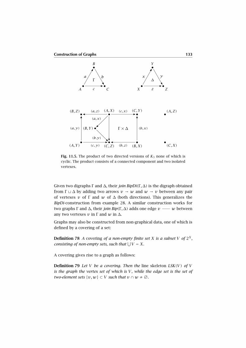
Construction of Graphs 133
B
CA
b
c
aΓ
Y
ZX
y
z
x∆
(A,X)(B,Z)
(A, Y) (C,Z) (B,X) (C,X)
(A,Z)(C, Y)
(B, Y)
(a, z)
(a,y)
(c,y) (b, z)
(b,x)
(c,x)
(a,x)
(b.y)
Γ ×∆
Fig. 11.5. The product of two directed versions of K3 none of which is
cyclic. The product consists of a connected component and two isolated
vertexes.
Given two digraphs Γ and ∆, their join BipDi(Γ ,∆) is the digraph obtained
from Γ t ∆ by adding two arrows v → w and w → v between any pair
of vertexes v of Γ and w of ∆ (both directions). This generalizes the
BipDi-construction from example 28. A similar construction works for
two graphs Γ and ∆, their join Bip(Γ ,∆) adds one edge v w between
any two vertexes v in Γ and w in ∆.
Graphs may also be constructed from non-graphical data, one of which is
defined by a covering of a set:
Definition 78 A covering of a non-empty finite set X is a subset V of 2X ,
consisting of non-empty sets, such that⋃V = X.
A covering gives rise to a graph as follows:
Definition 79 Let V be a covering. Then the line skeleton LSK(V) of V
is the graph the vertex set of which is V , while the edge set is the set of
two-element sets {v,w} ⊂ V such that v ∩w ≠∅.
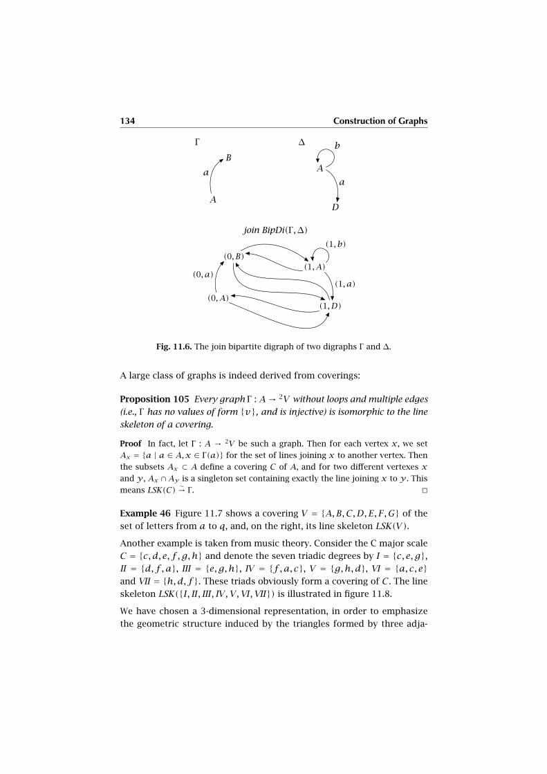
134 Construction of Graphs
ΓB
A
a
∆
A
D
a
b
join BipDi(Γ ,∆)
(0, B)
(0, A)
(0, a)(1, A)
(1,D)
(1, a)
(1, b)
Fig. 11.6. The join bipartite digraph of two digraphs Γ and ∆.
A large class of graphs is indeed derived from coverings:
Proposition 105 Every graph Γ : A→ 2V without loops and multiple edges
(i.e., Γ has no values of form {v}, and is injective) is isomorphic to the line
skeleton of a covering.
Proof In fact, let Γ : A → 2V be such a graph. Then for each vertex x, we set
Ax = {a | a ∈ A,x ∈ Γ(a)} for the set of lines joining x to another vertex. Then
the subsets Ax ⊂ A define a covering C of A, and for two different vertexes x
and y , Ax ∩Ay is a singleton set containing exactly the line joining x to y . This
means LSK(C)∼→ Γ . �
Example 46 Figure 11.7 shows a covering V = {A,B,C,D, E, F,G} of the
set of letters from a to q, and, on the right, its line skeleton LSK(V).
Another example is taken from music theory. Consider the C major scale
C = {c, d, e, f , g,h} and denote the seven triadic degrees by I = {c, e, g},II = {d, f ,a}, III = {e, g,h}, IV = {f ,a, c}, V = {g,h,d}, VI = {a, c, e}and VII = {h,d, f}. These triads obviously form a covering of C. The line
skeleton LSK({I , II , III , IV ,V ,VI ,VII}) is illustrated in figure 11.8.
We have chosen a 3-dimensional representation, in order to emphasize
the geometric structure induced by the triangles formed by three adja-
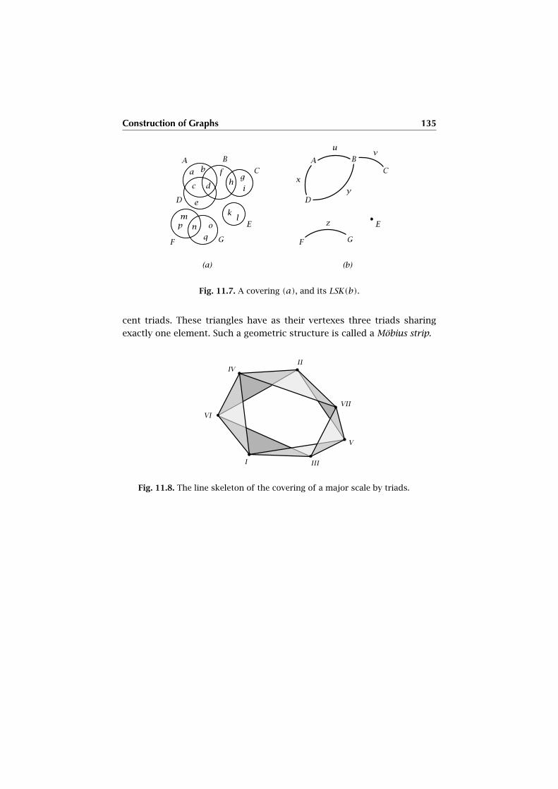
Construction of Graphs 135
Fig. 11.7. A covering (a), and its LSK(b).
cent triads. These triangles have as their vertexes three triads sharing
exactly one element. Such a geometric structure is called a Möbius strip.
Fig. 11.8. The line skeleton of the covering of a major scale by triads.
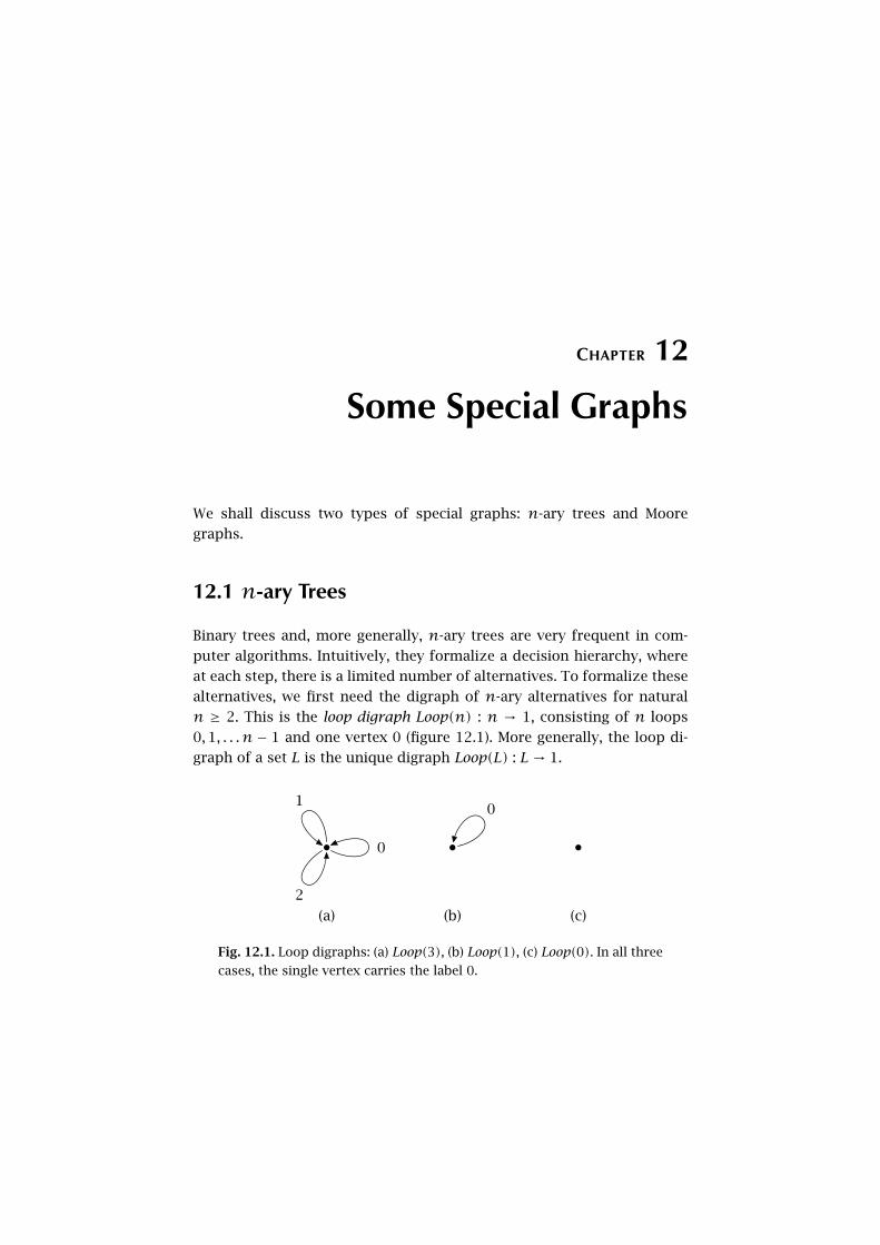
CHAPTER 12
Some Special Graphs
We shall discuss two types of special graphs: n-ary trees and Moore
graphs.
12.1 n-ary Trees
Binary trees and, more generally, n-ary trees are very frequent in com-
puter algorithms. Intuitively, they formalize a decision hierarchy, where
at each step, there is a limited number of alternatives. To formalize these
alternatives, we first need the digraph of n-ary alternatives for natural
n ≥ 2. This is the loop digraph Loop(n) : n → 1, consisting of n loops
0,1, . . . n − 1 and one vertex 0 (figure 12.1). More generally, the loop di-
graph of a set L is the unique digraph Loop(L) : L→ 1.
0
1
2
(a)
0
(b) (c)
Fig. 12.1. Loop digraphs: (a) Loop(3), (b) Loop(1), (c) Loop(0). In all three
cases, the single vertex carries the label 0.
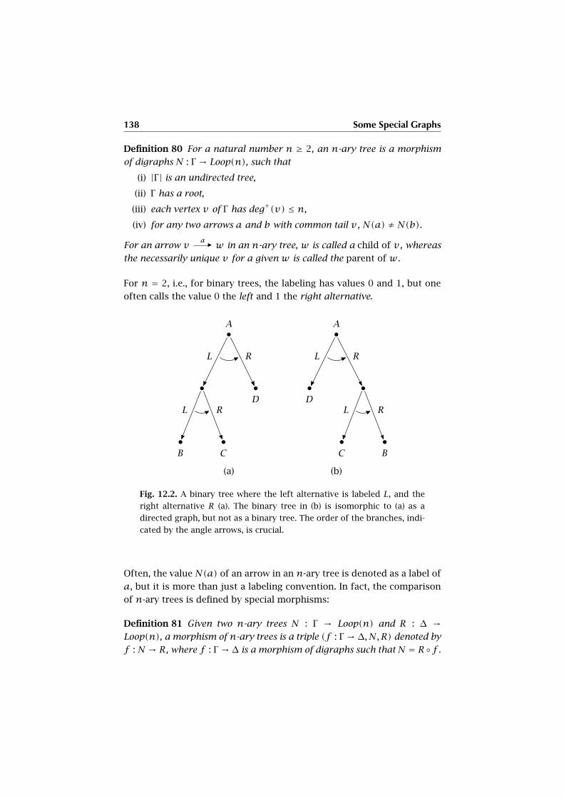
138 Some Special Graphs
Definition 80 For a natural number n ≥ 2, an n-ary tree is a morphism
of digraphs N : Γ → Loop(n), such that
(i) |Γ | is an undirected tree,
(ii) Γ has a root,
(iii) each vertex v of Γ has deg+(v) ≤ n,
(iv) for any two arrows a and b with common tail v , N(a) ≠ N(b).
For an arrow vañ w in an n-ary tree, w is called a child of v , whereas
the necessarily unique v for a given w is called the parent of w.
For n = 2, i.e., for binary trees, the labeling has values 0 and 1, but one
often calls the value 0 the left and 1 the right alternative.
L R
L R
A
B C
D
(a)
L R
L R
A
C B
D
(b)
Fig. 12.2. A binary tree where the left alternative is labeled L, and the
right alternative R (a). The binary tree in (b) is isomorphic to (a) as a
directed graph, but not as a binary tree. The order of the branches, indi-
cated by the angle arrows, is crucial.
Often, the value N(a) of an arrow in an n-ary tree is denoted as a label of
a, but it is more than just a labeling convention. In fact, the comparison
of n-ary trees is defined by special morphisms:
Definition 81 Given two n-ary trees N : Γ → Loop(n) and R : ∆ →Loop(n), a morphism of n-ary trees is a triple (f : Γ → ∆, N,R) denoted by
f : N → R, where f : Γ → ∆ is a morphism of digraphs such that N = R◦f .
12.2 Moore Graphs 139
In particular, for binary trees, this means that a left/right arrow of Γ must
be mapped to a left/right arrow of ∆. So it may happen that Γ and ∆ are
isomorphic digraphs without being isomorphic with the added n-labels
of alternatives.
12.2 Moore Graphs
A Moore graph is a special type of a process digraph as already presented
in a generic form in example 27. Moore graphs arise in the theory of
sequential machines and automata, which we introduce here since their
concepts are ideally related to the theory of digraphs thus far developed.
To begin with, we denote by Path(Γ) the set of paths in a digraph Γ ,
including the composition qp of paths p and q if possible (see exercise 45
for this construction). Also denote by Pathv(Γ) the set of paths starting at
vertex v . For a loop digraph Loop(A), the composition of any two paths
is possible and associative, moreover, the lazy path e at vertex 0 is a
“neutral element” for this composition, i.e., e ·p = p · e = p for any path
p ∈ Path(Loop(A)). This structure is also denoted by Word(A) and called
the word monoid over A (a justification for this terminology is given in
chapter 15). Any path p in Word(A) is defined by the (possibly empty)
sequence a1, . . . ak of its arrows (the letters of the word) from A since the
vertex 0 is uniquely determined. Further, If p = a1 . . . ak and q = b1 . . . bl,
the composition is exactly the concatenation of the letters of the two
words: q · p = b1 . . . bla1 . . . ak.
In automata theory, if n is a positive natural number, one considers
as “input set” the n-cube Qn = 2n, the elements of which are the “n-
bit words” such as w = (0,0,1,0,1,1, . . . ,1) (see also figure 13.3 on
page 146). For n = 1 the two words (0) and (1) are called bits, thus
elements of Qn are also defined as sequences of n bits. An 8-bit word
is called a byte. Evidently card(Qn) = 2n. The word monoid Word(Qn)
is called the input monoid, its elements are called tapes, so tapes in
Word(Qn) are just sequences consisting of n-bit words.
Definition 82 An automaton of n variables is a set function
A : Word(Qn)→ Q.
All automata can be constructed by a standard procedure which is de-
fined by sequential machines:
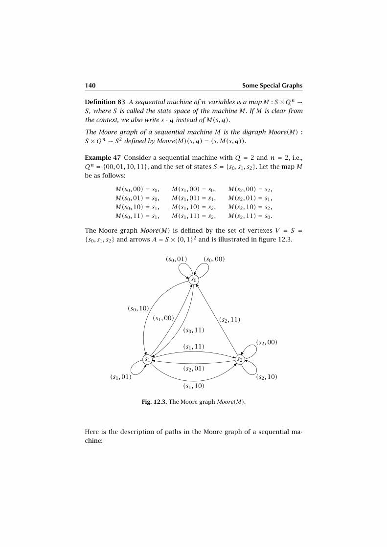
140 Some Special Graphs
Definition 83 A sequential machine of n variables is a map M : S ×Qn →S, where S is called the state space of the machine M . If M is clear from
the context, we also write s · q instead of M(s, q).
The Moore graph of a sequential machine M is the digraph Moore(M) :
S ×Qn → S2 defined by Moore(M)(s, q) = (s,M(s, q)).
Example 47 Consider a sequential machine with Q = 2 and n = 2, i.e.,
Qn = {00,01,10,11}, and the set of states S = {s0, s1, s2}. Let the map M
be as follows:
M(s0,00) = s0, M(s1,00) = s0, M(s2,00) = s2,M(s0,01) = s0, M(s1,01) = s1, M(s2,01) = s1,M(s0,10) = s1, M(s1,10) = s2, M(s2,10) = s2,M(s0,11) = s1, M(s1,11) = s2, M(s2,11) = s0.
The Moore graph Moore(M) is defined by the set of vertexes V = S ={s0, s1, s2} and arrows A = S × {0,1}2 and is illustrated in figure 12.3.
s0
s1 s2
(s0,00)(s0,01)
(s1,01)
(s2,00)
(s2,10)
(s0,10)
(s0,11)
(s1,00)
(s1,10)
(s1,11)
(s2,11)
(s2,01)
Fig. 12.3. The Moore graph Moore(M).
Here is the description of paths in the Moore graph of a sequential ma-
chine:
12.2 Moore Graphs 141
Proposition 106 For a sequential machine M : S ×Qn → S, a canonical
bijection
PW : Path(Moore(M)) → S ×Word(Qn)
is given as follows:
If
p = s1 (s1,q1)ñ s2
(s2,q2)ñ s3 · · · (sm−1,qm−1)
ñ sm,
then PW(p) = (s1, q1q2 . . . qm−1).
Under this bijection, for a given state s ∈ S, the set Paths(Moore(M)) cor-
responds to the set {s} ×Word(Qn).
Proof The map PW is injective since from the word q1q2 . . . qm−1 and the state
s1 we can read all the letters q1, q2, . . . qm−1, and then reach the other states
by s2 = s1q1, s3 = s2q2, . . . sm = sm−1qm−1. It is surjective, since for any pair
(s1, q1q2 . . . qm−1) the above reconstruction yields a preimage. The last statement
is immediate from the definition of PW . �
We are now ready to define automata associated with sequential ma-
chines. To this end, we fix a sequential machine M in n variables over
the state space S, an “initial” state s, and a so-called output function
O : S → Q. The automaton Automaton(M, s,O) : Word(Qn) → Q is de-
fined as follows. Denote by head : Paths(Moore(M)) → S : p , head(p)
the map associating with each path the head of its last arrow. Also denote
(s, ?) : Word(Qn)→ {s} ×Word(Qn) : w , (s,w). Then we define
Automaton(M, s,O) = O ◦ head ◦ PW−1 ◦ (s, ?) : Word(Qn)→ Q.
leads to the following result:
Proposition 107 For every automaton A, there is a sequential machineM ,
an initial state s, and an output function O such that
A = Automaton(M, s,O).
Proof In fact, given the automaton A : Word(Qn) → Q, take the state space
S = Word(Qn), the output function O = A and the sequential machine M :
S ×Qn → Q defined by M(s, q) = sq. With the initial state e (the empty word) we
have the automaton Automaton(M, e,A), and this is the given automaton O. �
Example 48 We revisit the sequential machine from example 47 and de-
fine the output function O : S → Q as:
142 Some Special Graphs
O(s0) = 0,
O(s1) = 1,
O(s2) = 1.
This yields an automaton A = Automaton(M, s0, O), where s0 has been
chosen as the “start” state. The result of A applied to the input sequence
10 10 00 01 11 ∈ Word(Qn) is computed as the value of the expression
O(head(PW−1((s0, ?)(10 10 00 01 11)))). Let us do this step by step:
1. (s0, ?)(10 00 01 01 11) = (s0,10 10 00 01 11) ;
2. PW−1(s0,10 10 00 01 11) is the path traced in the Moore graph of
figure 12.3 starting at s0 ; it is:
p = s0 (s0,10)ñ s1
(s1,10)ñ s2
(s2,00)ñ s2
(s2,01)ñ s1
(s1,11)ñ s2
3. head(p) = s2 ;
4. O(s2) = 1 .
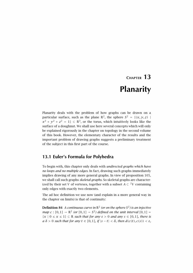
CHAPTER 13
Planarity
Planarity deals with the problem of how graphs can be drawn on a
particular surface, such as the plane R2, the sphere S2 = {(x,y, z) |x2 + y2 + z2 = 1} ⊂ R3, or the torus, which intuitively looks like the
surface of a doughnut. We shall use here several concepts which will only
be explained rigorously in the chapter on topology in the second volume
of this book. However, the elementary character of the results and the
important problem of drawing graphs suggests a preliminary treatment
of the subject in this first part of the course.
13.1 Euler’s Formula for Polyhedra
To begin with, this chapter only deals with undirected graphs which have
no loops and no multiple edges. In fact, drawing such graphs immediately
implies drawing of any more general graphs. In view of proposition 105,
we shall call such graphs skeletal graphs. So skeletal graphs are character-
ized by their set V of vertexes, together with a subset A ⊂ 2V containing
only edges with exactly two elements.
The ad hoc definition we use now (and explain in a more general way in
the chapter on limits) is that of continuity:
Definition 84 A continuous curve inR2 (or on the sphere S2) is an injective
map c : [0,1] → R2 (or [0,1] → S2) defined on the unit interval [0,1] ={x | 0 ≤ x ≤ 1} ⊂ R such that for any ε > 0 and any s ∈ [0,1], there is
a δ > 0 such that for any t ∈ [0,1], if |s − t| < δ, then d(c(t), c(s)) < ε,

144 Planarity
where the common Euclidean distance function d is defined by
d((x1, y1), (x2, y2)) =√(x1 − x2)2 + (y1 −y2)2.
Intuitively, continuity of such a curve means that you can draw the curve
from the beginning (curve parameter 0) to the end (curve parameter 1)
without lifting the pencil. We shall consider only continuous curves here
and omit this adjective in the following discussion. Denote by ]0,1[ the
unit interval without the two endpoints 0 and 1, the so-called interior of
the unit interval. Here is the definition of a drawing of a skeletal graph:
Definition 85 A drawing D of a skeletal graph Γ : A → 2V in X (where
X is commonly the plane R2, but can also be the sphere S2 or any more
general space, where continuity is reasonably defined) is given by D =(r , c = (ca)a∈A), where
(i) r : V → X is an injection,
(ii) for each edge vaw in A, there is a curve ca : [0,1] → X such
that
{ca(0), ca(1)} = r(Γ (a)),
(iii) for any two different edges a and b, the image ca(]0,1[) of the
interior of the first curve is disjoint from the image cb([0,1]) of the
entire second curve.
A skeletal graph is planar iff it has a drawing in R2.
The image⋃a∈A Im(ca) is denoted by D(Γ) and is called the drawn graph.
Remark 16 It is easy to prove this proposition: A graph has a drawing in
R2 iff it has a drawing in S2. The proof uses the stereographic projection,
known from geography, in fact a bijection S2 − NorthPole → R2, which
will be introduced in the chapter on topology. This implies that planarity
is equivalent to the existence of a drawing on the sphere S2.
A drawing of a connected skeletal graph on S2 is also called a polyhedron.
This is justified by the fact that if you are positioned within a polyhedron
(such as a cube or a tetrahedron), you see the edges of the polyhedron on
your visual sphere as if they were edges of a graph drawing on S2.
If D is a drawing of a skeletal graph Γ , then the complement R2 − D(Γ)of the drawn graph is the disjoint union of a number of regions which
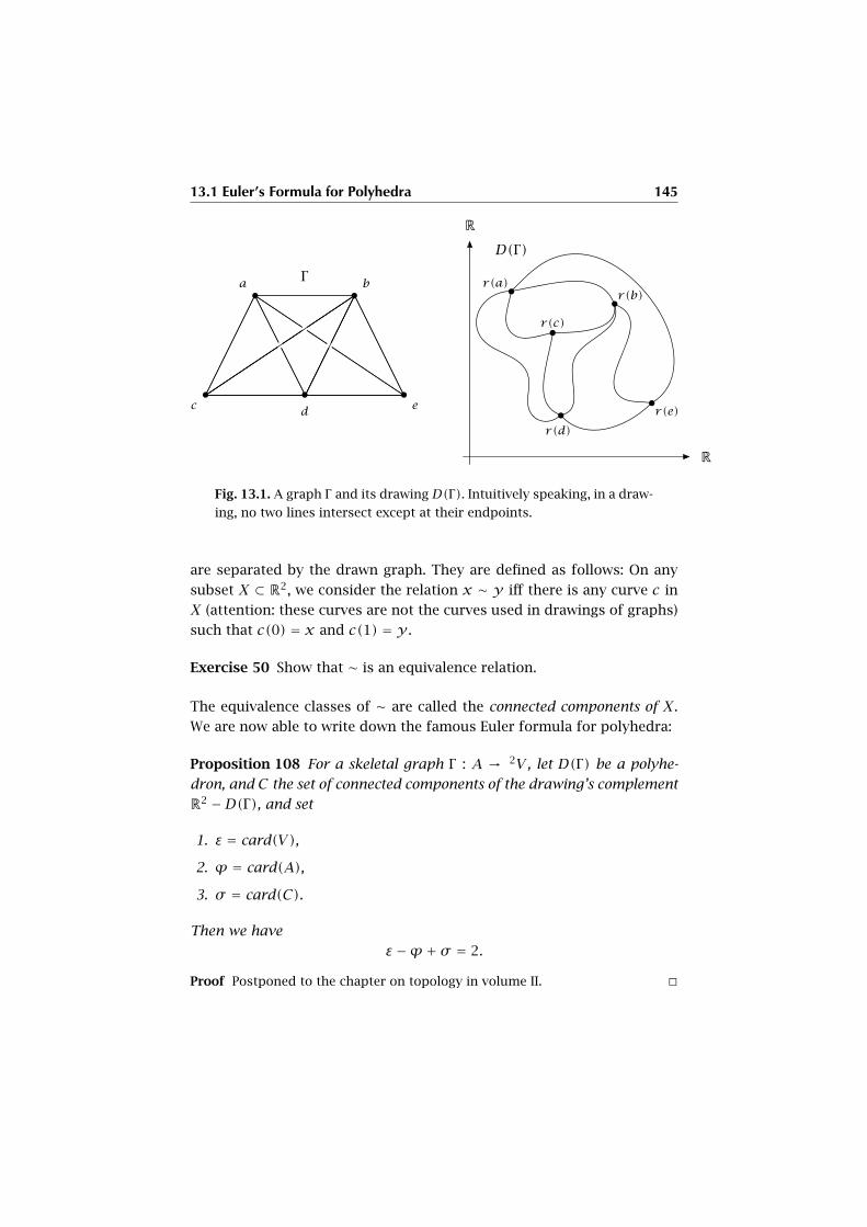
13.1 Euler’s Formula for Polyhedra 145
dc e
a bΓ
R
R
r(a)r(b)
r(c)
r(d)
r(e)
D(Γ)
Fig. 13.1. A graph Γ and its drawing D(Γ). Intuitively speaking, in a draw-
ing, no two lines intersect except at their endpoints.
are separated by the drawn graph. They are defined as follows: On any
subset X ⊂ R2, we consider the relation x ∼ y iff there is any curve c in
X (attention: these curves are not the curves used in drawings of graphs)
such that c(0) = x and c(1) = y .
Exercise 50 Show that ∼ is an equivalence relation.
The equivalence classes of ∼ are called the connected components of X.
We are now able to write down the famous Euler formula for polyhedra:
Proposition 108 For a skeletal graph Γ : A → 2V , let D(Γ) be a polyhe-
dron, and C the set of connected components of the drawing’s complement
R2 −D(Γ), and set
1. ε = card(V),
2. ϕ = card(A),
3. σ = card(C).
Then we have
ε −ϕ + σ = 2.
Proof Postponed to the chapter on topology in volume II. �

146 Planarity
x
yc
z
Fig. 13.2. The gray regions are the connected components of a graph.
Here x and y are in the same equivalence class, whereas x and z are
not.
Exercise 51 The n-cube Qn introduced in section 12.2 gives rise to the
n-cube graph, also denoted by Qn. It is a skeletal graph with vertex set
Qn and edges of the form {x,y}, where x and y differ exactly by one bit.
Find a drawing D of Q3. Show that in this case, the numbers in the Euler
formula are ε = 8,ϕ = 12, σ = 6.
Fig. 13.3. Hypercube Q4.
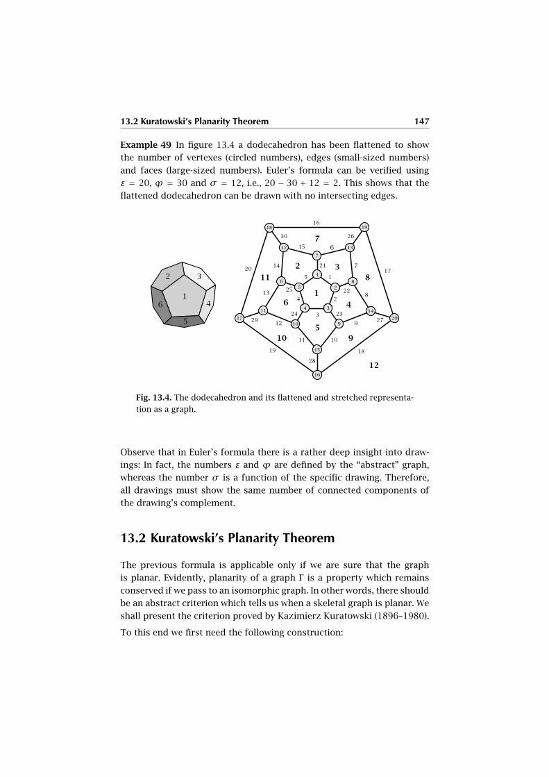
13.2 Kuratowski’s Planarity Theorem 147
Example 49 In figure 13.4 a dodecahedron has been flattened to show
the number of vertexes (circled numbers), edges (small-sized numbers)
and faces (large-sized numbers). Euler’s formula can be verified using
ε = 20, ϕ = 30 and σ = 12, i.e., 20 − 30 + 12 = 2. This shows that the
flattened dodecahedron can be drawn with no intersecting edges.
Fig. 13.4. The dodecahedron and its flattened and stretched representa-
tion as a graph.
Observe that in Euler’s formula there is a rather deep insight into draw-
ings: In fact, the numbers ε and ϕ are defined by the “abstract” graph,
whereas the number σ is a function of the specific drawing. Therefore,
all drawings must show the same number of connected components of
the drawing’s complement.
13.2 Kuratowski’s Planarity Theorem
The previous formula is applicable only if we are sure that the graph
is planar. Evidently, planarity of a graph Γ is a property which remains
conserved if we pass to an isomorphic graph. In other words, there should
be an abstract criterion which tells us when a skeletal graph is planar. We
shall present the criterion proved by Kazimierz Kuratowski (1896–1980).
To this end we first need the following construction:
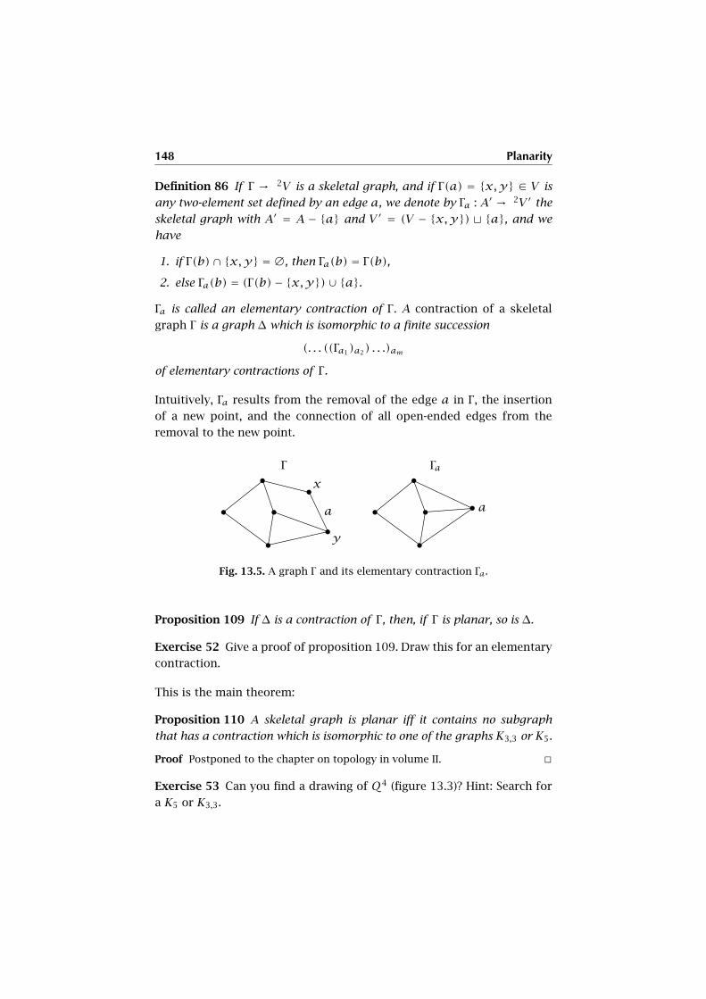
148 Planarity
Definition 86 If Γ → 2V is a skeletal graph, and if Γ(a) = {x,y} ∈ V is
any two-element set defined by an edge a, we denote by Γa : A′ → 2V ′ the
skeletal graph with A′ = A − {a} and V ′ = (V − {x,y}) t {a}, and we
have
1. if Γ(b)∩ {x,y} = ∅, then Γa(b) = Γ(b),2. else Γa(b) = (Γ(b)− {x,y})∪ {a}.
Γa is called an elementary contraction of Γ . A contraction of a skeletal
graph Γ is a graph ∆ which is isomorphic to a finite succession
(. . . ((Γa1)a2) . . .)am
of elementary contractions of Γ .
Intuitively, Γa results from the removal of the edge a in Γ , the insertion
of a new point, and the connection of all open-ended edges from the
removal to the new point.
x
y
a
Γ
a
Γa
Fig. 13.5. A graph Γ and its elementary contraction Γa.
Proposition 109 If ∆ is a contraction of Γ , then, if Γ is planar, so is ∆.
Exercise 52 Give a proof of proposition 109. Draw this for an elementary
contraction.
This is the main theorem:
Proposition 110 A skeletal graph is planar iff it contains no subgraph
that has a contraction which is isomorphic to one of the graphs K3,3 or K5.
Proof Postponed to the chapter on topology in volume II. �
Exercise 53 Can you find a drawing of Q4 (figure 13.3)? Hint: Search for
a K5 or K3,3.
CHAPTER 14
First Advanced Topic
14.1 Floating Point Arithmetic
In this section, we give an overview of computer-oriented arithmetic
based on the adic representation of real numbers as described in propo-
sition 92. Evidently, representation of numbers and arithmetic calcu-
lations on a computer are bounded by finite memory and time. Since
real numbers are based upon infinite information, computer arithmetic
must be limited to finite truncations of real arithmetic. Floating point
arithmetic is one approach to this problem. It is based on the well-
known approximative representation of real numbers in scientific con-
texts, such as Avogadro’s number N ≈ 6.02214× 10²³, Planck’s constant
h ≈ 6.6261 × 10⁻³⁴J s or the circle circumference number π ≈ 3.14159.
Here we consent that any number can be written as a small positive or
negative number f (in fact 1 ≤ |f | < 10 or f = 0 in the decimal system)
times a power 10e of the basis (here 10) for a positive or negative integer
exponent e. The term “floating point” stems from the difference to the
“fixed point” representation given in proposition 92 of chapter 9, where
the dot is relative to the 0-th power of the base, whereas here, the dot is
a relative information related to the variable power of the base.
Remark 17 Observe that the limitation to a finite number of digits in the
adic representation of real numbers implies that we are limited to special
rational numbers (not even 1/3 = 0.333 . . . is permitted in the decimal
system!). So why not just take the fractional representation which is a
precise one? The point is that, evidently, numerator and denominator of
150 First Advanced Topic
a fraction would also grow to unlimited size when doing arithmetic. So
the problem is not the fractional representation (though it would make
arithmetic precise in some cases), but the general program for calculating
with numbers within an absolutely limited memory space.
The IEEE (Institute for Electrical and Electronics Engineers) #754 standard
defines a specific way of floating point representation of real numbers. It
is specified for base 2 by a triple of (s, e, f ), where s ∈ {0,1} is the bit for
the sign, i.e., s = 0 iff the number is not negative, s = 1 iff it is negative.
The number e is the exponent and takes integer values e ∈ [−127,128],
corresponding to a range of 8-bits (28 = 256). The exponent is encoded
by a bias integer bias = 127. This means that we have to consider e−bias
instead of e in the computerized representation. The extra value −127
is set to 0. This exponent is reserved to represent number zero. We will
make this more precise in a moment. The maximal value e = 128, shifted
to 255 by the bias, is used to represent different variants of infinity and
“not-a-number” symbols. We therefore may vary the exponents in the in-
teger interval [−126,127]. In the binary representation using eight bits,
and with regard to the bias, this amounts to considering the zero num-
ber exponent symbol 00000000 whereas the infinities and not-a-number
symbols are represented by the maximum 11111111 (= 28 − 1 = 255).
So the exponent for common numbers takes shifted values in the binary
interval [00000001,11111110], corresponding to the unshifted interval
[−126,127].
The third number f is called the mantissa (an official, but mathematically
ill-chosen terminology) or fraction (non-official, but correct terminology,
also adapted by Knuth). We stick to the latter. The fraction f is encoded
in binary representation f = f1f2f3 . . . f23 ∈ [0,223 − 1], i.e., in binary
representation
00000000000000000000000 ≤ f1f2 . . . f23 ≤ 11111111111111111111111
and stands for the fraction 1.f = 1.f1f2 . . . f23 in binary representation.
Given these three ingredients, the number 〈s, e, f 〉 denoted by the triple
(s, e, f ) is the following real number:
〈s, e, f 〉 = (−1)s × 2e−bias × 1.f
This is the normalized floating point representation of the IEEE standard
#754. It is also called single precision representation since a finer repre-
sentation using two 32-bit words exists, but we shall not discuss this
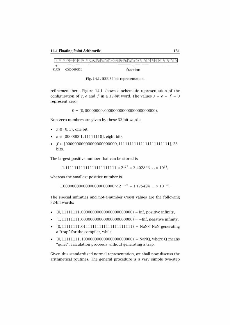
14.1 Floating Point Arithmetic 151
s e7 e6 e5 e4 e3 e2 e1 e0 f22f21f20f19f18f17f16f15f14f13f12f11f10 f9 f8 f7 f6 f5 f4 f3 f2 f1 f0
sign exponent fraction
Fig. 14.1. IEEE 32-bit representation.
refinement here. Figure 14.1 shows a schematic representation of the
configuration of s, e and f in a 32-bit word. The values s = e = f = 0
represent zero:
0 = (0,00000000,00000000000000000000000).
Non-zero numbers are given by these 32-bit words:
• s ∈ {0,1}, one bit,
• e ∈ [00000001,11111110], eight bits,
• f ∈ [00000000000000000000000,11111111111111111111111], 23
bits.
The largest positive number that can be stored is
1.11111111111111111111111× 2127 = 3.402823 . . .× 1038,
whereas the smallest positive number is
1.00000000000000000000000× 2−126 = 1.175494 . . .× 10−38.
The special infinities and not-a-number (NaN) values are the following
32-bit words:
• (0,11111111,00000000000000000000000) = Inf, positive infinity,
• (1,11111111,00000000000000000000000) = −Inf, negative infinity,
• (0,11111111,01111111111111111111111) = NaNS, NaN generating
a “trap” for the compiler, while
• (0,11111111,10000000000000000000000) = NaNQ, where Q means
“quiet”, calculation proceeds without generating a trap.
Given this standardized normal representation, we shall now discuss the
arithmetical routines. The general procedure is a very simple two-step

152 First Advanced Topic
algorithm: first, one of the operations of addition, subtraction, multipli-
cation, or division is performed, and then, in a second step, the result is
recast to the normalized representation shown above.
Regarding the first step, we shall only discuss addition, since the other
operations run in a completely similar way. To make the algorithm more
transparent, we use another (also Knuth’s, but not IEEE-standardized)
normalization by replacing the representation 1.f × 2e−bias by 0.1f ×2e−bias+1. Denote this representation by 〈〈s, e, g〉〉 = (−1)s × 2e−bias × gwith 0 ≤ g < 1, i.e., we have 〈s, e, f 〉 = 〈〈s, e + 1,0.1f 〉〉. Observe that
we now need 24 bits after the dot in order to represent this second nor-
malized representation. Observe also that the third coordinate g of the
second representation is the real number, including zero 0.0, and not just
the 23-bit word to the right of the dot as with the IEEE standard.
Given two normalized representations 〈〈su, eu, gu〉〉, 〈〈sv , ev , gv〉〉, the
computer calculation does not yield the exact sum, but an approxima-
tion 〈〈sw , ew , gw〉〉. In general, it is not normalized anymore. This will be
corrected by the subsequent normalization algorithm. However, the latter
will perform a further rounding error.
Here is the algorithm A for addition:
A.1: We check whether eu ≥ ev . If not, we exchange the summands and
proceed. As addition is commutative, this is a reasonable step, and
it will also be the reason why floating point addition is in fact com-
mutative.
A.2: Set ew = eu.
A.3: If eu−ev ≥ 24+2 = 26, we have a large difference of exponents, i.e.,
the smaller summand has its highest digit below the 24 digits admit-
ted in the normalized representation of 〈〈su, eu, gu〉〉. We therefore
set gw = gu. In this case, go to A.6. Actually, in this case, the result
is already normalized, and we could terminate the entire addition
here.
A.4: Divide gv by 2eu−ev , i.e., shift the binary representation by up to 9
places to the right. Attention: This procedure requires the computer
memory to hold up to 24+ 9 = 33 places temporarily.
14.1 Floating Point Arithmetic 153
A.5: Set gw = gu + gv . This last step gives us the correct sum
〈〈sw , ew , gw〉〉, but we have a gw which might not be normalized,
i.e., we could have gw ≥ 1.
A.6: Normalize, i.e., apply the normalization algorithm N to
〈〈sw , ew , gw〉〉.
The normalization algorithm N runs as follows, it converts a “raw” expo-
nent e and a “raw” fraction 0 ≤ g into a normalized representation.
N.1: If g ≥ 1 (fractional overflow), then go to step N.4. If g = 0, set e to
the lowest possible exponent in the normalized representation (in
fact e = −127 or 00000000 in the biased binary IEEE representation
and e = −126 in the second normalized representation).
N.2: (Normalization of g, i.e., g < 1 but large enough) If g ≥ 1/2, go to
step N.5.
N.3: (g is too small, but does not vanish) Multiply g by 2, decrease e by
1 and return to step N.2.
N.4: Divide g by 2 and increase e by 1 and return to step N.1.
N.5: (Round g to 24 places) This means that we want to change g to the
nearest multiple of 2−24. One looks at 224×g = . . . g−24.h and checks
the part h after the dot. According to whether h is less than 1/2 or
not, this part is omitted and 224 × g is replaced by . . . g−24.0 + 1 or
. . . g−24.0, see the following remark 18 for a comment. If the rounded
g is 1, return to step N.1.
N.6: (check e) If e is too large (more than 127), an exponent overflow
condition is sensed. If e is too small (less than −126 in the IEEE
standard, or less than−125 in the second normalized form 〈〈〉〉 used
in this algorithm), then an exponent underflow condition is sensed.
This concludes the normalization algorithm (except for the actions to be
taken for the over- and underflow situations).
Remark 18 There is an axiomatic version of this theory, where the round-
ing round(x) of a number x is given axiomatically with conditions
round(−x) = −round(x) and x ≤ y implies round(x) ≤ round(y). We
then define rounded arithmetic operations by u⊕v = round(u+v),u⊗v = round(u× v),u v = round(u− v),u� v = round(u/v).

154 First Advanced Topic
Attention: The floating point operations lose virtually all of the nice prop-
erties of the original operations. In particular, associativity and distribu-
tivity are lost. However, all floating point operations remain commutative
if the originals were so, in particular addition and multiplication with
floating point numbers are commutative. See [32].
14.2 Example for an Addition
Let u = 235.5 and v = 22.6 as an example for the addition algorithm. We
expect the result to be w = 258.1.
Binary representation
u = 1.110101110000000000000002 × 27
and
v = 1.0110100110011001100110 . . .2 × 24
Note that v cannot be exactly represented as a binary number with
finitely many non-vanishing digits: it is an infinite fraction with periodi-
cally recurring digits.
IEEE notation
u = 〈0, 1000 0110, 1101 0111 0000 0000 0000 000〉and
v = 〈0, 1000 0011, 0110 1001 1001 1001 1001 101〉Note that in this representation the last digit of v has been rounded up.
Knuth’s notation
u = 〈〈0, 1000 0101, 0.1110 1011 1000 0000 0000 0000〉〉and
v = 〈〈0, 1000 0010, 0.1011 0100 1100 1100 1100 1101〉〉
In particular
gu = 0.111010111000000000000000
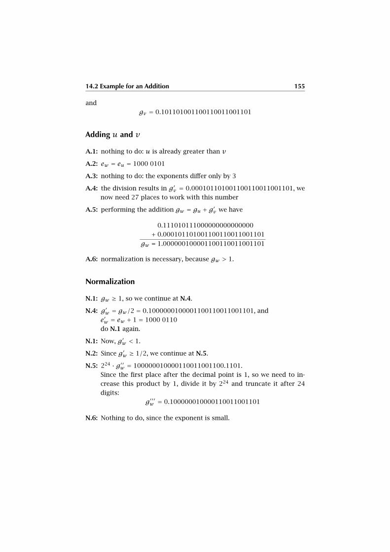
14.2 Example for an Addition 155
and
gv = 0.101101001100110011001101
Adding u and v
A.1: nothing to do: u is already greater than v
A.2: ew = eu = 1000 0101
A.3: nothing to do: the exponents differ only by 3
A.4: the division results in g′v = 0.000101101001100110011001101, we
now need 27 places to work with this number
A.5: performing the addition gw = gu + g′v we have
0.111010111000000000000000
+ 0.000101101001100110011001101
gw = 1.000000100001100110011001101
A.6: normalization is necessary, because gw > 1.
Normalization
N.1: gw ≥ 1, so we continue at N.4.
N.4: g′w = gw/2 = 0.1000000100001100110011001101, and
e′w = ew + 1 = 1000 0110
do N.1 again.
N.1: Now, g′w < 1.
N.2: Since g′w ≥ 1/2, we continue at N.5.
N.5: 224 · g′′w = 100000010000110011001100.1101.
Since the first place after the decimal point is 1, so we need to in-
crease this product by 1, divide it by 224 and truncate it after 24
digits:
g′′′w = 0.100000010000110011001101
N.6: Nothing to do, since the exponent is small.

156 First Advanced Topic
Knuth’s notation
Assembling the various parts (sw , e′w , g′′′w ) we get:
w = 〈〈0, 1000 0110, 0.1000 0001 0000 1100 1100 1101〉〉
IEEE notation
w = 〈0, 1000 0111, 0000 0010 0001 1001 1001 101〉
Binary representation
w = 1.000000100001100110011012 × 28
which translates to
1.00820314884185791015625× 256 = 258.100006103515625
Remark 19 The result of the addition algorithm is quite close, but not
exactly equal, to our expected result 258.1. This fact shows that calcula-
tions with floating point numbers are always only approximations.

PART II
Algebra, Formal Logic, and
Linear Geometry
CHAPTER 15
Monoids, Groups, Rings,
and Fields
This chapter introduces the indispensable minimal algebraic structures
needed for any further discussion, be it for formal logic and data struc-
tures, solving of linear equations, geometry, or differential calculus. The
students are asked to study this omnipresent material with particular
care.
We shall also see that many of the following structures have been en-
countered implicitly in the previous theory. We have encountered recur-
rent “laws” such as associativity, or identity properties. Therefore, the
following theory is also an exercise in abstraction, a essential activity in
computer science.
15.1 Monoids
Definition 87 A monoid is a pair (M,∗) where M is a set, and where
∗ : M ×M → M is a “composition” map satisfying these properties:
(i) (Associativity) For any triple k, l,m ∈ M , we have
(k∗ l)∗m = k∗ (l∗m),which we also write as k∗ l∗m.
(ii) (Neutral element) There is an element e ∈ M such that
m∗ e = e∗m =m
160 Monoids, Groups, Rings, and Fields
for allm ∈ M . Evidently, this element is uniquely determined by this
property. It is called the neutral element of the monoid.
A monoid (M,∗) is called commutative iff, for all m,n ∈ M ,
m∗n = n∗m.
Usually, we identify a monoid (M,∗) with its set M if the composition
∗ is clear. The notation of the product m ∗ n may vary according to the
concrete situation, sometimes even without any notation, such asmn for
m ∗ n. For commutative monoids, one often uses the symbol + instead
of ∗ and says that the monoid is additive.
Example 50 Denoting by ∗ the multiplication on N,Z,Q,R,C, these sets
define monoids, all of them commutative, with the number 1 being the
neutral element in each of them. They are usually called the multiplicative
monoids of these number domains.
The subset U = S(C) = {z | |z| = 1} of C is a monoid under ordinary
multiplication since |1| = 1 and |z ·w| = |z| · |w|, whence z ·w ∈ U if
z,w ∈ U . The monoid U is also called the unit circle.
Example 51 Given a set X, the set End(X) of set maps f : X → X, to-
gether with the usual composition of maps, is a monoid with neutral ele-
ment e = IdX . If we restrict the situation to the bijective maps in End(X),
we obtain a monoid Sym(X) (same neutral element). This monoid will
play a crucial role: We shall discuss it extensively in the following section
about groups.
Example 52 If Γ : A → V 2 is a directed graph, the set End(Γ) of endo-
morphisms of Γ , i.e., of morphisms f = (u,v) : Γ → Γ , together with the
composition ◦ of digraph morphisms, is a monoid. In general, this is not
a commutative monoid. We have a number of important special cases of
this construction.
To begin with, if the arrow set A of Γ is empty, the endomorphism monoid
identifies with the monoid End(V).
In section 12.2 on Moore graphs, we introduced the word monoid Word(A)
of a set A. A path p ∈ Word(A) is just a sequence of elements p =(a1, a2, . . . ak), and also the composition p = a1 · a2 · . . . ak of the paths
ai of length one. This is why this monoid is also called the word monoid
15.1 Monoids 161
over the alphabet A. A word is then a synonym for “path”, and the letters
of the word are the elements of A. The lazy path is called the empty word.
As with sets, where we introduced functions or set maps, we need the
formalism for comparing different instances of the monoid concept. Here
is the evident definition:
Definition 88 Given two monoids (M,∗M) and (N,∗N), a homomor-
phism f : (M,∗M)→ (N,∗N) is a set map f : M → N such that
(i) f(m∗M n) = f(m)∗N f(n) for all m,n ∈ M ,
(ii) f(eM) = eN for the neutral elements eM ∈ M and eN ∈ N.
Again, if the multiplications are clear, then we just write f : M → N to
denote a monoid homomorphism. The set of monoid homomorphisms f :
M → N is denoted by Monoid(M,N).
If we are given three monoids M,N,O and two monoid homomorphisms
f : M → N and g : N → O, their composition g ◦ f : M → O is defined by
the underlying set map composition, and this is also a monoid homomor-
phism.
Exercise 54 Show that the composition of three monoid homomor-
phisms, if defined, is associative, and that the identity map IdM : M → Mof any monoid M is a monoid homomorphism, the identity homomor-
phism of M .
Show that for a monoid homomorphism f : M → N the following state-
ments are equivalent:
(i) There is a homomorphism g : N → M such that
g ◦ f = 1M and f ◦ g = 1N ,
(ii) f is a bijection of sets.
A homomorphism satisfying these properties is called an isomorphism of
monoids. One says that two monoids M and N are isomorphic iff there
is an isomorphism f : M → N. The homomorphism g is uniquely deter-
mined and is called the inverse of f . It is denoted by g = f −1. If M = N(i.e., they are same as monoids, not only as sets), a homomorphism is
called an endomorphism. The set of monoid endomorphisms, together
with the composition of monoid homomorphisms and the identity on M ,
is itself a monoid and is denoted by End(M). An isomorphism which is
162 Monoids, Groups, Rings, and Fields
also an endomorphism is called automorphism. The subset of automor-
phisms in End(M) is also a monoid and is denoted by Aut(M).
Here is the “universal property” of the word monoid construction:
Proposition 111 (Universal Property of the Word Monoid) Let A be a
set, and N a monoid. Then the following map of sets is a bijection:
r : Monoid(Word(A),N)→ Set(A,N) : f , f |AProof The map r is injective since, if f(a) is given for all letters a ∈ A, then
f(a1 · a2 · . . . ak) = f(a1) · f(a2) · . . . f (ak), for any word a1 · a2 · . . . ak ∈Word(A), the empty path v must be mapped to the neutral element eN , and we
know f from its action on letters. Conversely, if g : A → N is a set map, define
f(a1 ·a2 · . . . ak) = g(a1)·g(a2)· . . . g(ak), which is well defined since the letters
of the word a1·a2·. . . ak are uniquely determined. Also, set f(v) = eN . Then this
yields a monoid homomorphism, since the multiplication of words is defined as
their concatenation. So r is surjective. �
The word monoid is therefore a kind of “free” object in the sense that any
“wild” map on its letters extends uniquely to a monoid homomorphism.
The so-called submonoids constitute a special type of homomorphisms:
Definition 89 If (M,∗) is a monoid with neutral element e, a submonoid
(M′,∗′) of M is a subset M ′ ⊂ M such that for all m,n ∈ M ′,m∗n ∈ M ′and e ∈ M ′, while the multiplication ∗′ is the restriction of ∗ to M ′. A
submonoid therefore gives rise to the evident embedding homomorphism
iM : M′ ↩ M .
Exercise 55 Given a monoid (M,∗) and a (possibly empty) subset S ⊂ M ,
there is a unique minimal submonoid M ′ of M such that S ⊂ M ′. It is
denoted by 〈S〉 and is called the submonoid generated by S. Show that
〈S〉 consists of all finite products s1∗s2∗ . . . sn, si ∈ S, and of the neutral
element e.
Example 53 We have plenty of submonoids among our previous exam-
ples (with the ordinary multiplications): N ⊂ Z ⊂ Q ⊂ R ⊂ C, U ⊂ C. If Γ
is a digraph, we have Aut(Γ) ⊂ End(Γ).
Exercise 56 The additive monoids, i.e., where ∗ is +, also define a chain
of submonoids N ⊂ Z ⊂ Q ⊂ R ⊂ C. If A is any set, the map l : Word(A)→(N,+) defined by the length of a word is a monoid homomorphism, i.e.,
l(pq) = l(p)+ l(q) and l(e) = 0.
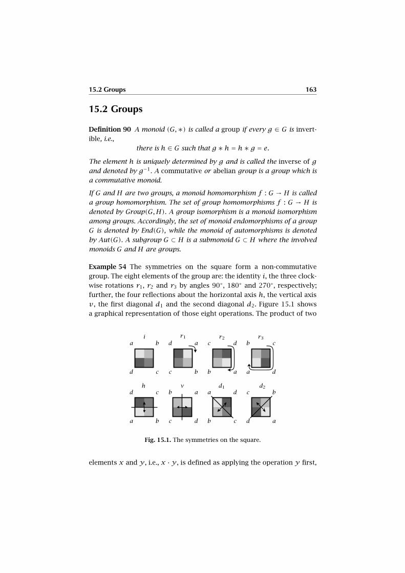
15.2 Groups 163
15.2 Groups
Definition 90 A monoid (G,∗) is called a group if every g ∈ G is invert-
ible, i.e.,
there is h ∈ G such that g ∗ h = h∗ g = e.The element h is uniquely determined by g and is called the inverse of g
and denoted by g−1. A commutative or abelian group is a group which is
a commutative monoid.
If G and H are two groups, a monoid homomorphism f : G → H is called
a group homomorphism. The set of group homomorphisms f : G → H is
denoted by Group(G,H). A group isomorphism is a monoid isomorphism
among groups. Accordingly, the set of monoid endomorphisms of a group
G is denoted by End(G), while the monoid of automorphisms is denoted
by Aut(G). A subgroup G ⊂ H is a submonoid G ⊂ H where the involved
monoids G and H are groups.
Example 54 The symmetries on the square form a non-commutative
group. The eight elements of the group are: the identity i, the three clock-
wise rotations r1, r2 and r3 by angles 90◦, 180◦ and 270◦, respectively;
further, the four reflections about the horizontal axis h, the vertical axis
v , the first diagonal d1 and the second diagonal d2. Figure 15.1 shows
a graphical representation of those eight operations. The product of two
Fig. 15.1. The symmetries on the square.
elements x and y , i.e., x ·y , is defined as applying the operation y first,

164 Monoids, Groups, Rings, and Fields
then x. The multiplication table for this group is shown in figure 15.2.
Although this group is not commutative, it has commutative subgroups,
for example {i, r1, r2, r3}.
· i r1 r2 r3 h v d1 d2
i i r1 r2 r3 h v d1 d2
r1 r1 r2 r3 i d1 d2 v h
r2 r2 r3 i r1 v h d2 d1
r3 r3 i r1 r2 d2 d1 h v
h h d2 v d1 i r2 r3 r1
v v d1 h d2 r2 i r1 r3
d1 d1 h d2 v r1 r3 i r2
d2 d2 v d1 h r3 r1 r2 i
Fig. 15.2. The multiplication table of the group of symmetries on the
square. The entry in row x and column y is the product x ·y
Example 55 The inclusion chain of additive monoids Z ⊂ Q ⊂ R ⊂ C are
all commutative groups. The set Z∗ = {1,−1} is a multiplicative group
in the multiplicative monoid Z. More generally, if (M,∗) is a monoid,
the subset M∗ of invertible elements in the sense of definition 90 is a
subgroup of M . It is called the group of invertible elements of M . Then
we have this inclusion chain of groups of invertible elements within the
multiplicative monoids of numbers: Z∗ ⊂ Q∗ ⊂ R∗ ⊂ C∗. Observe that
Z∗ = {−1,1}, Q∗ = Q− {0}, R∗ = R− {0}, and C∗ = C− {0}.
Exercise 57 Show that for a monoidM the submonoid Aut(M) ⊂ End(M)
is a group. Aut(M) is called the automorphism group of M .
The submonoid Sym(X) ⊂ End(X) of bijections of a set X is a very im-
portant group. It is called the symmetric group of X, its elements are
called the permutations of X. The permutation group of the interval
[1, n] = {1,2,3, . . . n} of natural numbers is called the symmetric group
of rank n and denoted by Sn.
Exercise 58 Show that, if card(X) = n is finite, then there is an isomor-
phism of groups Sym(X)∼→ Sn.
15.2 Groups 165
A permutation p ∈ Sn is best described by cycles. A cycle for p is a se-
quence C = (c1, c2, . . . ck) of pairwise different elements of [1, n] such
that p(c1) = c2, p(c2) = c3, . . .p(ck−1) = ck, p(ck) = c1, where k is called
the length of C and denoted by l(C). The underlying set {c1, c2, . . . ck}is denoted by |C|, i.e., l(C) = card(|C|). Conversely, each sequence
C = (c1, c2, . . . ck) of pairwise different elements of [1, n] denotes by def-
inition a permutation p such that p(c1) = c2, p(c2) = c3, . . . p(ck−1) =ck, p(ck) = c1, while the other elements of [1, n] are left fixed under p.
We also denote this p by C. Given such cycles C1, C2, . . . Cr , one denotes
by C1C2 . . . Cr the permutation C1 ◦ C2 ◦ . . . Cr . If a cycle C has length 2,
i.e., C = (x,y), then it is called a transposition, it just exchanges the two
elements x and y , and (x,y)(x,y) = Id.
Exercise 59 Let n = 4, take C1 = (124) and C2 = (23). Calculate the
permutation C1C2.
Proposition 112 Let p ∈ Sn. Then there is a sequence C1, C2, . . . Cr of
cycles of Sn such that
(i) the underlying sets |Ci| are mutually disjoint,
(ii) [1, n] = ⋃i |Ci|,(iii) p = C1C2 . . . Cr .
The sets |Ci| are uniquely determined by p, and for any two such repre-
sentations C1, C2, . . . Cr and C′1, C′2, . . . C
′r of p, if |Ci| = |C′j|, then there
is an index 1 ≤ t ≤ l = l(Ci) = l(C′j) such that Ci = (c1, c2, . . . cl) and
C′j = (ct , ct+1, . . . cl, c1, c2, . . . ct−1).
This representation of p is called the cycle representation.
Proof If such a cycle representation of p exists, then if i ∈ Cj , then Cj ={pk(i) | k = 0,1,2 . . .}, and conversely, every such so-called orbit set {pk(x) |k = 0,1,2 . . .} defines the cycle containing x. So the cycles are identified by these
orbits which are defined uniquely by p. Such sets define a partition of [1, n]. In
fact, if {pk(i) | k = 0,1,2 . . .} ∩ {pk(i′) | k = 0,1,2 . . .} ≠ ∅, then there are k
and k′ such that pk(i) = pk′(i′). Suppose k ≥ k′. Then multiplying by (p−1)k′,
we obtain pk−k′(i) = i′, i.e., the orbit of i′ is contained in that of i. But since
Sn is finite, not all powers p,p2, p3, . . . can be different. If pl = pl+t , t ≥ 1,
then by multiplication with (p−1)l, we have pt = Id, i.e., p−1 = pt−1. Therefore
pk′−k(i′) = (p−1)k−k′(i′) = (pt−1)k−k′(i′) = i, and both orbits coincide. So the
cycle representation is the uniquely determined orbit representation, which is a
partition of [1, n], thus (i) and (ii) follow.

166 Monoids, Groups, Rings, and Fields
Part (iii) follows since the cycles act like p on their elements. The last statement
is clear. �
Exercise 60 Beside the cycle representation of permutations, a tabular
representation can be used, where an element on the top line is mapped
to the element below it. Find the cycle representation for the following
permutations:
1 2 3 4 5 6 7 8
4 6 5 8 7 2 3 1∈ S8
1 2 3 4 5 6
6 1 4 2 5 3∈ S6
Definition 91 The cardinality of a group G is called the order of G, it is
denoted by ord(G). A group with finite order is called a finite group. A
group G with ord(G) = 1 is called trivial.
Exercise 61 Show that any two trivial groups are isomorphic.
Definition 92 If n ∈ N, we define n! = 1 if n = 0, and n! = 1·2·3·4· . . .nelse. The number n! is called n-factorial.
Exercise 62 Give a rigorous inductive definition of n!.
Proposition 113 If n ∈ N, then
ord(Sn) = n!
Proof The image i = p(n) of n under a permutation p ∈ Sn can be any of the n
elements in [1, n]. The other elements in [1, n − 1] are sent to the complement
[1, n]− {i} having n− 1 elements. By induction, this gives (n− 1)! possibilities,
and we have n · ((n− 1)!) = n!, as required, and since the induction start n = 1
is evident, we are done. �
The following result is a fundamental tool for constructing subgroups of
a given group:
Proposition 114 Let X ⊂ G be any subset of a group G. Then there is a
unique minimal subgroup H of G such that X ⊂ H. The group H consists
of the neutral element e of G and of all finite products x1 ∗ x2 ∗ . . . xk,where either xi ∈ X or xi = y−1
i , yi ∈ X. The subgroup H is denoted by
〈X〉 and is called the subgroup generated by (the elements of) X.
If there is a finite set X ⊂ G such that G is generated by X, i.e., G = 〈X〉,then G is called a finitely generated group. In particular, if X = {x}, one
writes G = 〈x〉 and calls G a cyclic group.

15.2 Groups 167
Proof The uniqueness of the minimal subgroup H results from the fact that for
any non-empty family (Gi)i of subgroups of G, their intersection⋂iGi is a sub-
group of G. The family of all subgroups Gi containing X is not empty (G is in the
family), so the intersection is this unique minimal subgroup H. Clearly, H con-
tains all finite products of the described type. Moreover, this set is a subgroup,
the inverse of a product x1 ∗ x2 ∗ · · ·xk being x−1k ∗ x−1
k−1 ∗ . . . x−11 , which is of
the required type. �
Exercise 63 Find some 2-element sets that generate the group of symme-
tries on the square (see figures 15.1 and 15.2). Can you state a necessary
condition for a 2-element set to generate the group?
Definition 93 For an element x of a group G, the order of 〈x〉 is called
the order of x.
Proposition 115 If n ≥ 2 is a natural number, then Sn is generated by the
set {(1, k) | k = 2,3, . . . n} of transpositions. Since a transposition has or-
der 2, any x ∈ Sn can be written as a product x = (1, k1)(1, k2) . . . (1, kr ).
The subset An of the elements x ∈ Sn which can be written as a product
of an even number (a multiple of 2) of transpositions is a subgroup of Sn
of order n!/2. It is called the alternating group of rank n.
Proof For n = 2, Sn is obviously generated by (1,2). For the general case n > 2,
let p(n) = i for a given permutation p ∈ Sn. Then (i,n)p fixes n and is an ele-
ment of Sn−1. Therefore, by induction, it is a product of transpositions (1, r ), r <
n. But (i,n) = (1, i)(1, n)(1, i), so p = (i,n)(i,n)p = (1, i)(1, n)(1, i)((i,n)p),and we are done.
Clearly, An is a subgroup. If (1, i) is any transposition, then An → Sn : p ,
(1, i)p is an bijective map from An to the set Bn of permutations which are
products of an odd number of transpositions. If we can show that An ∩ Bn =∅, then Sn is the disjoint union of An and Bn, and therefore Sn = An t Bn,
whence card(An) = n!/2. To show this, given a permutation p, denote by i(p) =(i1, i2, . . . in) the sequence with j = p(ij). Let s(p) be 1 if the number of pairs
u < v such that iu > iv in i(p) is even, and −1 if it is odd. Clearly, s(Id) = 1.
If (i, i + 1) is a transposition of neighboring numbers, then evidently s((i, i +1) · p) = −s(p) Moreover, a general transposition (i, j) is the product of an odd
number of transpositions (k, k+ 1) of neighboring numbers. In fact, if j = i+ 1,
we are done, and for j > i+ 1, we have (i, j) = (i, k)(k, j)(i, k) for i < k < j, so
our claim follows by induction. Therefore s((i, j)) = −1. If p is a product of r
transpositions, we have s(p) = −1r , and r cannot be even and odd at the same
time. So An ∩ Bn = ∅. �
168 Monoids, Groups, Rings, and Fields
The alternating group An is a typical example of a group construction
which has far-reaching consequences for all mathematical theories which
involve groups, and this is virtually the entire mathematical science. The
observation is that An is related to a particular group homomorphism
sig : Sn → Z∗ defined by sig(x) = 1 if x ∈ An, and sig(x) = −1 else
(verify that sig is indeed a group homomorphism). The point is that, by
definition, An = {x ∈ Sn | sig(x) = 1}, i.e., An is the subgroup of ele-
ments being sent to the neutral element 1 of the codomain group. The
systematic context is this:
Definition 94 The kernel of a group homomorphism f : G → H is the
subgroup Ker(f ) = {x ∈ G | f(x) = eH}.The image of f is the set-theoretic image Im(f ), a subgroup of H.
Proposition 116 A group homomorphism f is an injective map iff its ker-
nel is trivial.
Proof If f is injective, then Ker(f ) = f−1(e) must be a singleton, so it is triv-
ial. Conversely, if Ker(f ) = e, then f(x) = f(y) implies e = f(x)f(y)−1 =f(x)f(y−1) = f(xy−1) = e, whence xy−1 = e, there x = y . �
Therefore we have An = Ker(sig). But there is more: We have two equipol-
lent complementary subsets An and Sn−An of the full group Sn, and the
image group Z∗ is of order 2. This suggests that we may try to recon-
struct the codomain group from the domain group and the kernel group.
This can effectively be done, but we need a small preliminary discussion.
Definition 95 Given a subgroup H ⊂ G and an element g ∈ G, the left
H-coset of g is the set gH = {gh | h ∈ H} . The set of left H-cosets of G is
denoted by G/H. The right H-coset is the set Hg = {hg | h ∈ H}. The set
of right H-cosets of G is denoted by H\G.
Sorite 117 Given a subgroup H ⊂ G, we have these facts:
(i) The relation “x ∼ y iff x ∈ yH” is an equivalence relation, where
the equivalence classes are the left cosets, i.e., two cosets are either
disjoint or equal, and G/H = G/∼. Each left coset gH is equipollent
with H by means of h, gh. This means that we have a set bijection
G/H ×H ∼→ G.
(ii) The relation “x ∼ y iff x ∈ Hy” is an equivalence relation, the
equivalence classes are the right cosets, i.e., two cosets are either
15.2 Groups 169
disjoint or equal, andH\G = G/∼. Each right cosetHg is equipollent
with H by means of h , hg. We have a set bijection H\G ∼→ G/H,
and therefore also H\G ×H ∼→ G.
The common cardinality of G/H or H\G is denoted by (G : H) and
is called the index of H in G.
(iii) Let G be a finite group, then we have the Lagrange equation
card(G) = card(H) · (G : H).
In particular, the order of any subgroupH of a finite groupG divides
the order of G. More specifically, if x ∈ G is any element and if G is
finite, then the order of x divides the order of G.
Proof (i) The relation x ∼ y means that x = yh, for some h ∈ H. Taking h = e,we obtain x ∼ x, and from x = yh one deduces y = xh−1, i.e., y ∼ x. Finally,
x = yh and y = zk, k ∈ H, implies x = zkh, whence x ∼ z.
The surjection fg : H → gH : h , gh, g ∈ G, is an injection because f −1g (gh) =
fg−1(gh) = g−1(gh) = h. So G/H ×H ∼→ G. The proof of (ii) works similarly with
“left” and “right” being exchanged.
The Lagrange equation (iii) now follows from (ii) since card(G) = card(G/H ×H) = card(G/H) · card(H) = (G : H) · card(H). �
The kernel of a homomorphism is more than a subgroup, it is exactly
such that the set of cosets G/H can be made into a group in a canonical
way.
Proposition 118 Let H be a subgroup of a group G. Then the following
properties are equivalent:
(i) There is a group K and a group homomorphism f : G → K such
that H = Ker(f ).
(ii) Left and right cosets coincide, i.e., for all x ∈ G, xH = Hx.The
composition xH · yH = xyH then defines a group structure, the
quotient group, on G/H. The group H is the kernel of the group
homomorphism G → G/H : x , xH.
Proof (i) implies (ii): If H = Ker(f ), then for every x ∈ G and every h ∈ H,
f(xhx−1) = f(x)f(h)f(x−1) = f(x)f(x−1) = f(x)f(x)−1 = e, so xHx−1 ⊂ H,
but also x−1Hx ⊂ H, whence xHx−1 = H, i.e., xH = Hx, for all x.
(ii) implies (i): The composition xH · yH = xyH is well defined since if xH =x′H, then xyH = xHy = x′Hy = x′yH, and if yH = y ′H, then xyH = xy ′H.
It is a group composition having H as neutral element and x−1H as the inverse

170 Monoids, Groups, Rings, and Fields
of xH. The map f : G , G/H : g , gH is a surjective homomorphism, and
gH = H iff g ∈ H. So H = Ker(f ). �
Definition 96 A subgroup H ⊂ G with the equivalent properties of propo-
sition 118 is called a normal subgroup of G; the group G/H is called the
quotient group of G modulo H.
Taking proposition 118 (i) with G = Sn, H = An, K = Z∗ and f = sig, we
see that the alternating group An is a normal subgroup of Sn.
Exercise 64 Show that every subgroup of a commutative group is nor-
mal. For example, given n ∈ N, we consider the additive subgroup
〈n〉 ⊂ Z. Show that this is the group consisting of all multiples z·n,z ∈ Zof n; therefore, we also write Z ·n for 〈n〉.
Definition 97 The quotient group Z/(Z ·n) is denoted by Zn and is called
the cyclic group of order n. Its order is indeed n. In fact, by the Euclidean
division theorem, every integer w is written uniquely in the form w =q·n+r ,0 ≤ r < n. Therefore every coset is of the form r+Z·n, 0 ≤ r < n,
and if r +Z·n = r ′+Z·n, then r = r ′+q ·n, therefore q = 0, and r ′ = r .
If we deal with elements of Zn, they are represented by cosets r +Z. Often,
one makes calculations on Zn but works with such representatives. In order
to tell that two representatives r , s ∈ Z represent the same coset, one writes
r ≡ s mod n or r ≡ s (mod n) or else r ≡ s (n) or even r = s(n).
We are now ready for the reconstruction of the image Im(f ) of a group
homomorphism f by means of the domain group and the kernel Ker(f ):
Proposition 119 If f : G → H is a group homomorphism, there is a canon-
ical isomorphism of groups
p : G/Ker(f )∼→ Im(f )
given by p(gKer(f )) = f(g) and satisfying the following commutative
diagram:
Gf
ñ H
G/Ker(f )� ∼
ñ Im(f )
�
15.3 Rings 171
Proof The map p : G/Ker(f ) → Im(f ) is well defined since gKer(f ) = hKer(f )
iff g−1h ∈ Ker(f ), so e = f(g−1h) = f(g−1)f (h), i.e., f(g) = f(h). It is sur-
jective by construction and also a group homomorphism by the definition of the
quotient group. Its kernel is the set of those cosets gKer(f ) such that f(g) = e,i.e., g ∈ Ker(f ), i.e., gKer(f ) = Ker(f ), the neutral element of the quotient
group G/Ker(f ). So by proposition 116 it is injective. �
Example 56 Reconsidering the homomorphism sig : Sn → Z∗, we know
that Ker(sig) = An, and Im(sig) = Z∗. Therefore, by proposition 119,
Sn/An∼→ Z∗.
15.3 Rings
Although groups are fundamental to mathematics, their structure is
somewhat too poor for realistic applications. We have seen in chapter 9
that the important number domains Z,Q,R,C share a simultaneous pres-
ence of two kinds of operations: addition and multiplication. We have
even learned that the very construction of the real numbers needs the
auxiliary space of Cauchy sequences, which also shares addition and mul-
tiplication with the other spaces. Here is the precise statement about the
common properties of these combined operations:
Definition 98 A ring is a triple (R,+,∗) such that (R,+) is an additive
abelian group with neutral element 0R (or 0 if the context is clear), and
where (R,∗) is a multiplicative monoid with neutral element 1R (or 1 if
the context is clear). These two structures are coupled by the distributivity
laws:
for all x,y, z ∈ R, x ∗ (y + z) = x ∗y + x ∗ zand (x +y)∗ z = x ∗ z +y ∗ z.
One refers to (R,+) when referring to the additive group of a ring and
to (R,∗) when referring to the multiplicative monoid of the ring. Usually,
one simply writes R for the ring (R,+,∗) if addition and multiplication are
clear from the context. The group of multiplicatively invertible elements of
a ring is denoted by R∗. If the context is clear, then one often writes ab or
a · b or a.b instead of a∗ b.
A ring is commutative iff its multiplicative monoid is so.

172 Monoids, Groups, Rings, and Fields
A subring of a ring is a ring which is simultaneously an additive subgroup
and a multiplicative submonoid.
Example 57 As already announced, we have a number of prominent rings
from previous theory. If we denote by + and ∗ the ordinary addition and
multiplication, respectively, in the number domains Z,Q,R and C, then
each of (Z,+,∗), (Q,+,∗), (R,+,∗), and (C,+,∗) is a commutative ring.
Moreover, the set of Cauchy sequences C, together with the sum and
product of Cauchy sequences, is a commutative ring.
The additive cyclic groups (Zn,+) can also be turned into commutative
rings by defining the multiplication (r +n · Z)∗ (s +n · Z) = rs +n · Z.
Evidently, this multiplication is well defined, since two representations
r ≡ r ′ (mod n) have their difference in n · Z.
Exercise 65 Verify that multiplication in Zn is well defined. What is the
multiplicative neutral element 1Zn?
Rings are also related to each other by ring homomorphisms:
Definition 99 A set map f : R → S of rings R and S is a ring homomor-
phism if f is a group homomorphism of the additive groups of R and S
and if f is a monoid homomorphism of the multiplicative monoids of R and
S. The set of ring homomorphisms from R to S is denoted by Ring(R, S).
The composition of two ring homomorphisms f : R → S and g : S → Tis the set-theoretic composition g ◦ f . The properties of group and monoid
homomorphisms imply that composition is also a ring homomorphism.
An isomorphism f of rings is a homomorphism of rings which is an
isomorphism of additive groups and of multiplicative monoids (which is
equivalent to the condition that f is a bijective set map). An endomor-
phism or rings is a homomorphisms of one and the same ring. A ring
automorphism is an endomorphism which is an isomorphism of rings.
Example 58 The inclusions Z ⊂ Q ⊂ R ⊂ C are ring homomorphisms.
The conjugation ? : C∼→ C is an automorphism of C. The canonical maps
Z→ Zn are ring homomorphisms.
Example 59 A crucial construction of rings which are not commutative
in general is the so-called “monoid algebra”. A very important special case
15.3 Rings 173
is the omnipresent polynomial ring, so the following construction is far
from an academic exercise.
To construct a monoid algebra, we need a commutative ring (R,+, ·) and
a monoid (M,∗). The monoid algebra of R andM is the following ring: Its
set is the subset R〈M〉 of the set RM consisting of all functions h : M → Rsuch that h(z) = 0R for all but a finite number of arguments z ∈ M . Given
a pair (r ,m) ∈ R×M , the special function f : M → R with f(m) = r and
f(n) = 0 for all n ≠ m is denoted by r ·m. The addition on R〈M〉 is
defined by (f +g)(m) = f(m)+g(m). Clearly this function evaluates to
0R for all but a finite number of arguments if f and g do so. The product
is defined by (f · g)(m) = ∑n,t g(n) · f(t), where the sum is taken over
the finite number of pairs (n, t) such that n∗ t =m and either g(n) or
f(t) differs from 0R. If there is no such non-zero value, the product is
defined to be the zero function 0R · eM .
Exercise 66 Given a ring R and a monoid M as above, show that the
monoid algebra R〈M〉 defined in example 59 is a ring with additive neu-
tral element 0R · eM and multiplicative neutral element 1R · eM . It is com-
mutative iff M is so. Every element f ∈ R〈M〉 can be written as a finite
sum f =∑i=1,...k fi ·mi = f1 ·m1+f2 ·m2+ . . . fk ·mk, with fi = f(mi).
If f ≠ 0, the the summands fi ·mi are uniquely determined up to per-
mutations if one only adds up those with fi ≠ 0. One therefore also uses
the notation f = ∑m fm ·m where it is tacitly supposed that only a finite
number of summands is considered, of course comprising only those m
where f(m) ≠ 0.
There is an injective ring homomorphism R → R〈M〉 : r , r · eM , and
an injective homomorphism M → R〈M〉 : m , 1R ·m of multiplicative
monoids. One therefore also identifies elements of R and M their respec-
tive images in the monoid algebra. We observe that under this identifica-
tion, any two elements r ∈ R and f ∈ R〈M〉 commute, i.e., r · f = f · r .
This is the theoretical reason why the word “R-algebra” comes into this
construction.
Example 60 If in particular M = Word(A) is the word monoid of an
alphabet A, then the monoid algebra is called the R-algebra of non-
commutative polynomials in the indeterminates from A. So every ele-
ment is a sum of so-called monomials r · X1X2 . . . Xk in the indeter-
minates Xi ∈ A. In particular, if A = {X1, X2, . . . Xn} is a finite set of
174 Monoids, Groups, Rings, and Fields
so-called “indeterminates” Xi, then the monoid algebra is denoted by
R〈X1, X2, . . . Xn〉.The most prominent such algebra is the case for A = {X}. We then get
the words Xk = XXX . . .X, the k-fold juxtaposition of the unique letter
X. A polynomial in the indeterminate X is then written in the form
f = rk ·Xk + rk−1 ·Xk−1 + rk−2 ·Xk−2 + . . . r2 ·X2 + r1 ·X + r0,
or else f(X) in order to put the indeterminate X in evidence. The monoid
algebra is then commonly denoted by R[X] instead of R〈X〉. Compare
addition and multiplication of such polynomials in X to what you know
from high school mathematics.
For a non-zero polynomial in X, the maximal power Xk of X such that the
coefficient rk is different from zero is called the degree of f , in symbols
deg(f ), and rk is called the leading coefficient.
In particular, if the degree of f is 3 the polynomial f(X) is called cubic, if
it is 2, then f(X) is called quadratic, if it is 1, then f(X) is called linear,
and if f(X) = r0 ∈ R, then f(X) is called a constant polynomial.
Remark 20 Consider the monoid ComWord(A) whose elements are equi-
valence classes of words over A in the sense that w ∼ w ′ iff the words’
letters are just permutations of each other. Then the product of words
from Word(A) is well defined on equivalence classes, which are also
called commutative words. Taking the monoid ComWord(A), the monoid
algebra is commutative and is denoted by R[A] = R〈ComWord(A)〉. It
is called the R-algebra of commutative polynomials in the indeterminates
from A.
The power of the monoid algebra construction is shown in this proposi-
tion:
Proposition 120 (Universal Property of Monoid Algebras) Let R be a
commutative ring, M a monoid, and S a (not necessarily commutative)
ring. Suppose that f : R → S is a ring homomorphism such that for all
r ∈ R and s ∈ S, f(r) · s = s ·f(r). Then for any monoid homomorphism
µ : M → S into the multiplicative monoid of S, there is exactly one ring
homomorphism f 〈µ〉 : R〈M〉 → S which extends f and µ, i.e., f 〈µ〉|R = fand f 〈µ〉|M = µ.
15.3 Rings 175
Proof On an argument∑m gm ·m, any ring homomorphism f 〈µ〉 which extends
f and µ as required, must be defined by f 〈µ〉(∑m gm ·m) =∑m f 〈µ〉(gm) ·
f 〈µ〉(m) = ∑m f(gm) · µ(m). But this is a well defined map since the sum
representation of the argument is unique. It is now straightforward to check
that this map is indeed a ring homomorphism. �
The most important consequence of this proposition is this corollary:
Corollary 121 If R is a commutative ring, and if {X1, X2, . . . Xn} is a finite
set, then every set map v : Xi , xi ∈ R extends to a ring homomorphism
R〈v〉 : R〈X1, X2, . . . Xn〉 → R, whose value on a monomial r ·Xi1Xi2 . . . Xikis r ·xi1xi2 . . . xik . This homomorphism is called the evaluation of polyno-
mials with respect to v .
Proof This follows at once from proposition 111 and proposition 120, applying
the universal property of the word monoid over the symbols Xi to obtain µ, and
the universal property of a monoid algebra for f = IdR and µ. �
Example 61 If f = f(X) = rk·Xk+rk−1·Xk−1+rk−2·Xk−2+. . . r2·X2+r1·X+r0 is a polynomial in C[X], then the map X , x ∈ C defines the evalu-
ation f(x) = rk·xk+rk−1·xk−1+rk−2·xk−2+. . . r2·x2+r1·x+r0 of f(X)
at x. This means that a polynomial f(X) defines a function f(?) : C→ C,
which is called a polynomial function. Generally speaking, a polynomial
function is simply a function defined by a polynomial and an evaluation
of its indeterminates, as guaranteed by the above proposition 120.
In analogy to normal subgroups, which are the kernels of group homo-
morphisms, it is possible to define structures which are the kernels of
ring homomorphisms. We shall only need the theory for commutative
rings. Here is the characterization:
Proposition 122 Let J be an additive subgroup of a commutative ring R.
Then the following properties are equivalent:
(i) There is a homomorphism of commutative rings f : R → S such that
J = Ker(f ) for the underlying additive groups.
(ii) J is a subgroup of the additive group of R, and for every r ∈ R,
if x ∈ J, then r · x ∈ J. The multiplication (x + J) · (y + J) =xy + J defines the multiplication of a ring structure on the quotient
group R/J, the quotient ring. The group J is the kernel of the ring
homomorphism R → R/J : x , x + J.
176 Monoids, Groups, Rings, and Fields
Proof The proof is completely analogous to that regarding normal subgroups
and kernels of group homomorphisms. We leave it as an exercise to the reader. �
Definition 100 A subgroup J ⊂ R with the equivalent properties of propo-
sition 122 is called an ideal of R.
Example 62 We are now capable to better understand the construction of
the ring of real numbers R from Cauchy sequences. The set C of Cauchy
sequences as defined in definition 50 is a commutative ring, this is state-
ment (i) in proposition 79, together with the constant sequence (1)i as
multiplicative neutral element, while statements (i) and (ii) in proposi-
tion 79 tell us that the zero sequences O define an ideal. Finally, by
lemma 81, the equivalence relation in lemma 80 is precisely the relation
defined by the ideal O, and the quotient structure C/O is the same as the
structure defined in definition 54.
Example 63 Reconsidering the construction of the cyclic groups Zn, we
recognize that the subgroup Z·n of Z is in fact an ideal. The construction
of the ring multiplication on the quotient group Z/(Z · n) is exactly the
one we just defined for the quotient ring.
The type of ideal in the previous example is of major importance for the
theory of prime numbers and follows from the Euclidean algorithm:
Definition 101 An ideal J of a commutative ring R is called a principal
ideal if there is an element x ∈ J such that J = R · x = {r · x | r ∈ R}.Such an ideal is also denoted by J = (x). A ring the ideals of which are all
principal is called a principal ideal ring.
Proposition 123 The ring Z is a principal ideal ring. If J is an ideal of Z,
then either J = (0) or J = (n), where n ∈ N is the smallest positive integer
in J.
Proof If J is an non-zero ideal in Z, then there is a smallest positive element
n in J. For any j ∈ J, we have j = an + b, 0 ≤ b < n, by elementary natural
arithmetic. But then b = j − an ∈ J, whence b = 0, therefore J = (n). �
We also have the analogous ring-theoretic proposition analogous to propo-
sition 119 for groups:
Proposition 124 If f : R → S is a homomorphism of commutative rings,
there is a canonical isomorphism of rings
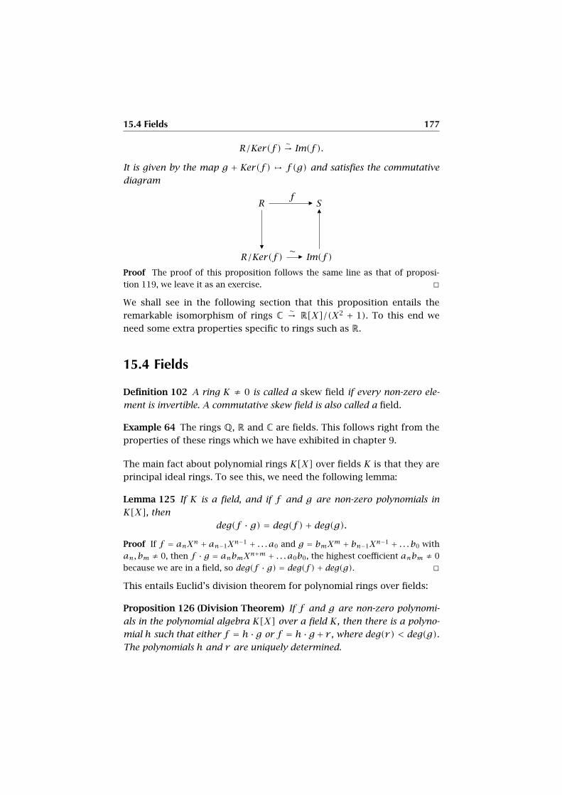
15.4 Fields 177
R/Ker(f )∼→ Im(f ).
It is given by the map g + Ker(f ) , f(g) and satisfies the commutative
diagram
Rf
ñ S
R/Ker(f )� ∼
ñ Im(f )
�
Proof The proof of this proposition follows the same line as that of proposi-
tion 119, we leave it as an exercise. �
We shall see in the following section that this proposition entails the
remarkable isomorphism of rings C∼→ R[X]/(X2 + 1). To this end we
need some extra properties specific to rings such as R.
15.4 Fields
Definition 102 A ring K ≠ 0 is called a skew field if every non-zero ele-
ment is invertible. A commutative skew field is also called a field.
Example 64 The rings Q, R and C are fields. This follows right from the
properties of these rings which we have exhibited in chapter 9.
The main fact about polynomial rings K[X] over fields K is that they are
principal ideal rings. To see this, we need the following lemma:
Lemma 125 If K is a field, and if f and g are non-zero polynomials in
K[X], then
deg(f · g) = deg(f )+ deg(g).
Proof If f = anXn + an−1Xn−1 + . . . a0 and g = bmXm + bn−1X
n−1 + . . . b0 with
an, bm ≠ 0, then f · g = anbmXn+m + . . . a0b0, the highest coefficient anbm ≠ 0
because we are in a field, so deg(f · g) = deg(f )+ deg(g). �
This entails Euclid’s division theorem for polynomial rings over fields:
Proposition 126 (Division Theorem) If f and g are non-zero polynomi-
als in the polynomial algebra K[X] over a field K, then there is a polyno-
mial h such that either f = h ·g or f = h ·g+ r , where deg(r) < deg(g).
The polynomials h and r are uniquely determined.
178 Monoids, Groups, Rings, and Fields
Proof Let deg(f ) < deg(g), then f = 0 · g + f is a solution. If deg(f ) ≥ deg(g),
then for f = anXn + an−1Xn−1 + . . . a0 and g = bmXm + bn−1X
n−1 + . . . b0,
we consider f ′ = f − anbmXn−m · g. The polynomial f ′ has smaller degree than
f , and we may proceed by induction to find a solution f ′ = h′ · g + r ′. Then
f = ( anbmXn−m+h′) ·g+ r ′ solves the problem. As to uniqueness, if we have two
decompositions f = h1 · g + r1 = h2 · g + r2, then (h1 −h2) · g = r2 − r1, which,
for reasons of degree, only works if h1 − h2 = r2 − r1 = 0. �
Example 65 To compute the quotient and remainder of the division of
2X4+4x3+17x2+13x+23 by 2x2+5, the tabular method can be used:
2x4 + 4x3 + 17x2 + 13x + 23 : 2x2 + 5 = x2 + 2x + 6
2x4 + 5x2
4x3 + 12x2 + 13x
4x3 + 10x
12x2 + 3x + 23
12x2 + 30
3x +−7
Thus, the quotient is x2 + 2x + 6 and the remainder is 3x − 7.
The Division Theorem implies the announced result:
Proposition 127 If K is a field, then the polynomial ring K[X] is a prin-
cipal ideal ring. If J is an ideal of K[X], then either J = (0) or J = (g),where g is a polynomial in J of minimal degree.
Proof In fact, the proof works like for integers. Take a minimal polynomial f of
positive degree in an ideal J, then by proposition 126, J = (f ). �
We may now demonstrate the announced isomorphism between C and
R[X]/(X2 + 1). Consider the ring homomorphism v : R[X] → C defined
by the natural embedding R ⊂ C and the evaluation X , i = √−1. Clearly,
v is surjective, i.e., Im(v) = C. The kernel of v is a principal ideal ring,
Ker(v) = (t). But no non-zero linear polynomial a·X+b is in this kernel,
since a · i + b = 0 iff a = b = 0. On the other hand, X2 + 1 ∈ Ker(v),
therefore by proposition 127, Ker(v) = (X2+1). By proposition 124, this
implies R[X]/(X2 + 1)∼→ C.
Exercise 67 Using the isomorphism R[X]/(X2 + 1)∼→ C, try to describe
the conjugation on C by means of the quotient ring R[X]/(X2 + 1).
15.4 Fields 179
For both constructions, that of R from Cauchy sequences, and that of C
from polynomials over R, we are left with the question: Why do these
quotient rings yield fields? Here is the answer:
Definition 103 A proper ideal J of a commutative ring R is called maxi-
mal if there is no ideal I such that J Ð I Ð R.
Proposition 128 An ideal J is maximal in R iff the quotient R/J is a field.
Proof If J is not maximal, than a strictly larger ideal I such that J Ð I Ð R has an
image I′ in R/J which is a proper ideal such that 0 Ð I′ Ð R/J, so R/J cannot be
a field. In fact, suppose that R/J is a field and take x ≠ 0 ∈ I ′. Take its inverse
x−1. Then, since I′ is an ideal, x−1x = 1 is an element of I′. Therefore I′ = R/J. If
J is maximal, then any x 6∈ J must generate the improper ideal R together with
J, in particular there are u ∈ R and v ∈ J such that 1 = ux + v . Then the image
1 + J = ux + J = (u + J) · (x + J), i.e., every non-zero element x + J in R/J is
invertible, and we have a field. �
Now, the missing links are easily inserted:
Example 66 The ideal (X2+1) in R[X] is maximal. In fact, a strictly larger
ideal must be of shape (X + a), but then we must have the factorization
X2+1 = (X+a)·(X+b). Evaluating (X2+1) at x = −a yields a2+1 = 0, an
impossibility in R. Turning to Cauchy sequences, any non-zero sequence
(ai)i has a sequence (bi)i such that (ai)i · (bi)i converges to 1, this was
shown in statement (viii) of sorite 84. So every ideal which is strictly larger
than O must be the principal ideal (1), i.e., the entire ring, and we are
done.
CHAPTER 16
Primes
This chapter is devoted to prime numbers and prime polynomials, a type
of objects which play an important role in cryptography. Every computer
scientist should therefore have some knowledge about prime factoriza-
tion in the ring of integers Z and the polynomial algebras K[X] over one
indeterminate X with coefficients in a field K.
16.1 Prime Factorization
We first need a small preliminary discussion about the construction of
ideals by generators, a generalization of the concept of a principal ideal
introduced in the last chapter.
Definition 104 If G ⊂ R is a non-empty subset of a commutative ring R,
the ideal generated by G is defined as the set of all sums r1 ·g1 + r2 ·g2 +. . . rk · gk where gi ∈ G and ri ∈ R. It is denoted by (G) or (h1, h2, . . . ht)
if G = {h1, h2, . . . ht} is finite.
Exercise 68 Show that that the set (G) is indeed an ideal.
Here is the definition of a prime element in a commutative ring:
Definition 105 A non-zero element p ∈ R in a commutative ring R is
prime if it is not invertible and if p = q · r implies that either q or r
is invertible. For polynomial algebras, prime polynomials are also called
irreducible.
182 Primes
To begin with, we make sure that in the most interesting rings, every
non-invertible element has a factorization into prime elements:
Lemma 129 If R = Z or R = K[X], where K is a field, then every non-
invertible element x ≠ 0 has a factorization x = p1 · p2 · . . . pk as a
product of primes pi.
Proof For a non-invertible, non-zero p ∈ Z, we proceed by induction on |p| ≥ 2.
A factorization p = q · r implies |p| = |q| · |r |. So if |p| = 2, then p = ±2 is
already prime, since one of its factors in 2 = q · r must be 1. In the general
case, a factorization p = q · r with non-invertible factors implies |q|, |r | < |p|,so by induction on these factors, we are done. For a non-invertible, non-zero
p ∈ K[X], we proceed by induction on deg(p) ≥ 1. A factorization p = q · rimplies deg(p) = deg(q)+ deg(r). If deg(p) = 1, then either q or r is a constant
(degree zero), and therefore invertible. If deg(p) > 1, then if all factorizations
have either q or r of degree zero, then these factors are invertible and p is prime.
Else, degrees decrease and induction applies to the factors. �
One could imagine that there is only a finite number of primes. But we
have the classical result about prime numbers in Z, Euclid’s theorem:
Proposition 130 The set of primes in Z is infinite.
Proof Suppose that p1 = 2, p2 = 3, . . . pk is the finite set all positive primes
in Z. Then the prime factorization of q = 1 +∏i=1,2,...k pi must contain one of
these primes, say pt . Then we have q = pt ·u = 1+∏i=1,2,...k pi, and therefore1
1 = pt · (u −∏i=1,2,...t,...k pi), which is impossible since pt is not invertible by
hypothesis. So there are infinitely many primes in Z. �
Example 67 In particular 0R is not prime since 0R = 0R · 0R, and 1R,−1Rare not prime since they are invertible. The numbers ±2, ±3, ±5, ±7, ±11,
±13,±17,±19 in Z are primes, while 12,−24,15 are not. In R[X] all linear
polynomials a·X+b,a ≠ 0, and all quadratic polynomials a·X2+b with
a,b > 0 are prime. (Use the argumentation from example 66 to prove
that X2 + 1 = (u ·X + v)(r ·X + s) is impossible in R[X].)
Clearly, prime factorization is not unique because of the commutativ-
ity of the ring and the existence of invertibles, e.g., 12 = 2 · 2 · 3 =1 The convention xi means that in an indexed sequence, the object xi
with index i is omitted, and only the earlier and later terms are consid-
ered. For example, x1, x2, x3, . . . x9, . . . x20 means that we take the sequence
x1, x2, x3, . . . x8, x10, . . . x20.
16.1 Prime Factorization 183
3 · (−2) · (−2). However, this is the only source of ambiguities in prime
factorization for our prominent rings.
Definition 106 If x and y are two elements in a commutative ring such
that there is an element z with y = x · z, then we say that x divides y
or that x is a divisor of y and write x|y . If x does not divide y , we write
x ö y . Clearly, x|y is equivalent to the inclusion (y) ⊂ (x) of ideals.
If 0 = x · y for x,y ≠ 0, then x is called a zero divisor. A commutative
ring without zero divisors is called an integral domain.
Lemma 131 In an integral domain R, the generator of a principal ideal a
is unique up to invertible elements, i.e., (a) = (b) iff there is c ∈ R∗ such
that b = c · a.
Proof Clearly the existence of such an c ∈ R∗ is sufficient. Conversely, (a) = (b)implies a = xb and b = ya, whence a = xya, i.e., xy = 1 if a ≠ 0. But if a = 0,
then also b = 0 and we have discussed all cases. �
Notation 10 If R is a principal integral domain, the ideal generated by
two elements a and b is principal, i.e., (a, b) = (d). This is equivalent to
the two facts that (1) d|a and d|b, (2) there are two elements u and v such
that d = u · a + v · b. Such a d is called the greatest common divisor of
a and b, in symbols d = gcd(a, b). The ideal (a) ∩ (b) is also principal,
(a) ∩ (b) = (l). This means that (1) a|l and b|l, (2) whenever a|x and
b|x, then l|x. Such an l is called the least common multiple of a and b,
in symbols l = lcm(a, b). Observe that gcd and lcm are only determined
up to invertible elements.
Proposition 132 (Euclidean Algorithm) For two integers a and b the
gcd(a, b) is calculated by this recursive algorithm:
gcd(a, b) ={a if b = 0
gcd(b, r) otherwise
where r is determined by the Division Theorem: a = q · b + r (proposi-
tion 68).
Proof Suppose that we have this chain of successive divisions:

184 Primes
a = q1 · b + r1,
b = q2 · r1 + r2,
r1 = q3 · r2 + r3,
r2 = q4 · r3 + r5,
...
rk = qk+2 · rk+1.
Then the claim is that rk+1 = gcd(a, b). In fact, clearly rk+1|a and rk+1|b, by suc-
cessive replacement in these formulas from the end. Moreover, each remainder
r1, r2, etc. is a combination u ·a+v ·b, and so is in particular the last, i.e., rk+1,
whence the proposition. �
Example 68 Using the Euclidean Algorithm, the greatest common divisor
of 17640 and 462 is calculated as follows:
17640 = 38 · 462+ 84
462 = 5 · 84+ 42
84 = 2 · 42
a = q1 · b + r1
b = q2 · r1 + r2
r1 = q3 · r2
Therefore, gcd(17640,462) = 42.
Example 69 Fields and all subrings of fields are integral domains. In
particular, all the rings Z,Q,R,C are integral domains, and so are the
polynomial algebras K[X] over a field K, because formula deg(f · g) =deg(f ) + deg(g) guarantees that f · g ≠ 0 for non-zero polynomials f
and g.
Remark 21 The converse is also true: Any integral domain is a subring
of a field.
Lemma 133 If the principal ideal ring R is an integral domain, then an
ideal I is maximal iff there is a prime p with I = (p). If q is another prime
with I = (q), then there is an invertible element e such that q = e · p.
Proof If I = (p) is maximal, then p = q · r implies (p) ⊂ (q), so either (q) = R,
and q ∈ R∗, or else (p) = (q), whence r ∈ R∗, therefore p is prime. If I is not
maximal, there is q such that I Ð (q) Ð R, i.e., p = q · r , and q, r 6∈ R∗, therefore
p is not prime. �
Proposition 134 For a positive prime number p ∈ Z, the finite ring Zp is
a field. In particular, the multiplicative group Z∗p has p − 1 elements, and

16.1 Prime Factorization 185
therefore for every integer x, we have xp ≡ x mod (p), and xp−1 ≡ 1
mod (p) if p ö x. The latter statement is called Fermat’s little theorem.
Proof The finite ring Zp is a field by lemma 133. By the Langrage equation from
sorite 117, the order of an element x ∈ G divides the order of G. Since the order
of Z∗p is p − 1, we have xp−1 = 1. �
The next result leads us towards the uniqueness property of prime fac-
torization:
Proposition 135 Let R be a principal integral domain and p ∈ R prime.
Then if p|a1 · a2 · . . . an, then there is an index i such that p|ai.Proof In fact, by lemma 133, R/(p) is a field, and therefore, the fact that p|a1 ·a2 · . . . an yields 0 = a1 · a2 · . . . an in the field R/(p), but this implies that one
of these factors vanishes, i.e., p divides one of the factors ai. �
Proposition 136 Let R be a principal integral domain. Then, if an element
a has two prime factorizations a = p1 · p2 · . . . pk = q1 · q2 · . . . ql, then
k = l, and there is a permutation π ∈ Sk and a sequence e1, e2, . . . ek of
invertible elements such that qi = ei · pπ(i), i = 1,2, . . . k.
Proof This is clear from the preceding proposition 135 if we take the factoriza-
tion q1 ·q2 · . . . ql and a divisor pj of this product. This means pj = ei ·qi for an
invertible ei. Then, dividing everything by pj reduces to a shorter product, and
we proceed by induction. �
Proposition 137 In Z, every non-invertible element a ≠ 0 has a unique
factorization by positive primes p1 < p2 < . . . pr and positive powers
t1, t2, . . . tr of the form
a = ±pt11 · pt22 · . . . ptrr .
Proof This follows directly from the above proposition 136, when ordering the
prime numbers by size. �
Corollary 138 In the polynomial algebra K[X] over a field K, every poly-
nomial of positive degree is a product of irreducible polynomials, and this
factorization is unique in the sense of proposition 136. In particular, every
linear polynomial is irreducible.
Proof This follows from the existence of a prime factorization after lemma 129
and the uniqueness statement in proposition 136. �
186 Primes
Remark 22 It can be shown that in C[X], the irreducible polynomials are
exactly the linear polynomials. This means that every polynomial f(X) of
positive degree is a product f(X) = a(X −b1)(X −b2) . . . (X −bk), a ≠ 0.
This is a quite profound theorem, the so-called fundamental theorem of
algebra.
Exercise 69 Show that√
2 is not a rational number. Use the prime factor-
ization of numerator a and denominator b in a fictitious representation√2 = a
b .
Exercise 70 Use exercise 69 to show that the set Q(√
2) consisting of the
real numbers of form z = a√2+b, with a,b ∈ Q, is a subfield of R. Show
that Q(√
2)∼→ Q[X]/(X2 − 2).
16.2 Roots of Polynomials and Interpolation
In this section, let K be a field. Let x ∈ K. Then we know from example 61
that for a polynomial f(X) ∈ K[X], there is an evaluation f(x) ∈ K. We
now want to discuss the relation between the polynomial f(X) and the
polynomial function f(?) : K → K : x , f(x).
Definition 107 If f(X) ∈ K[X], then an element x ∈ K is a root of f(X)
if f(x) = 0.
Lemma 139 If x ∈ K is a root of a polynomial f(X) ∈ K[X], then (X −x)|f(X).Proof We have the division with remainder f(X) = Q(X) · (X − x) + c, c ∈ K.
The evaluation of f at x yields c = 0, whence the claim. �
Proposition 140 If x1, x2, . . . xr are r different roots of f(X) ∈ K[X],then
(X − x1)(X − x2) . . . (X − xr )|f(X).In particular, a non-zero polynomial f(X) has at most deg(f ) different
roots.
Proof The proof uses induction on r . By the above lemma 139, the claim is true
for r = 1. But since each X − xr is prime and differs from all X − xj , j ≠ i, we
have a factorization f(X) = g(X) · (X − xr ). So all xi, i < r are roots of g(X),
and by the induction hypothesis, we are done. �
16.2 Roots of Polynomials and Interpolation 187
Corollary 141 If two polynomials f , g ∈ K[X] of degrees deg(f ) < n and
deg(g) < n agree on n different argument values xi, i = 1,2, . . . n, i.e.,
f(xi) = g(xi), then f = g.
Proof This is an easy exercise using proposition 140. �
Corollary 142 If for K = Q,R,C, two polynomial functions f(?) and g(?)
coincide, then the polynomials f(X), g(X) ∈ K[X] are equal.
Proof This follows from the fact that we have infinitely many arguments, where
the functions coincide. �
This allows us to identify polynomials and their associated functions,
but this is only a special situation, which does not generalize to arbitrary
polynomial algebras.
As an example that the fact stated in corollary 142 is not valid for K = Z2,
consider the polynomials f(X) = X2 + 1 and g(X) = X + 1 in Z2[X].
Evidently, f(X) and g(X) are different regarded as polynomials, but
f(0) = g(0) = 1, and f(1) = g(1) = 0, and thus are equal regarded
as polynomial functions.
We have not yet determined if there is always a polynomial f(X) of de-
gree strictly less than n such that its values f(xi) = yi can be prescribed
for n different arguments x1, x2, . . . xn. This is indeed guaranteed by var-
ious so-called interpolation formulas, the best known being those by La-
grange and Newton. Since the result must be unique by corollary 141, we
may pick one such formula.
Proposition 143 (Newton Interpolation Formula) Suppose that we are
given a sequence (x1, y1), (x2, y2), . . . (xn, yn) of couples (xi, yi) ∈ K2
for a field K, where xi ≠ xj for i ≠ j. Then there is a (necessar-
ily unique) polynomial f(X) ∈ K[X] of degree deg(f ) < n such that
f(xi) = yi, i = 1,2, . . . n. It is given by the Newton interpolation formula
f(X) = a0 + a1(X − x1)+ a2(X − x1)(X − x2)+ . . .an−1(X − x1)(X − x2) . . . (X − xn−1).
Exercise 71 Give a proof of proposition 143. Start with the evaluation at
x1 and calculate the coefficient a0. Then proceed successively with the
calculation of all coefficients a1, a2, . . . an−1.

188 Primes
Why are such formulas called “interpolation formulas”? The point is that
we are often given a series of “values” yi for arguments xi, but we do
not know which function f : K → K takes these values, yi = f(xi). In
most cases there is a large number of solutions for this problem. Any
solution, such as the polynomial solution given in proposition 143, will
also give us values for all other x ∈ K. For example, if K = R, we get all
the evaluations f(x) for the intervals x ∈ [xi, xi+1]. This means that f
can also be evaluated on values ‘between’ the given arguments, which is
the very meaning of the word ‘interpolation’.
Example 70 Given are the four points p1 = (−2,3), p2 = (−12 ,−1
2), p3 =(1, 1
2) and p4 = (2,−1) in R2. The goal is to construct the interpolation
polynomial f(X) ∈ R[X] through these points. Proposition 143 ensures
that f(X) is of the form:
f(X) = a0 + a1(X − x1)+ a2(X − x1)(X − x2)+a3(X − x1)(X − x2)(X − x3)
Now, setting X = xi and f(X) = yi for i = 1,2,3,4, the aj for j = 0,1,2,3
are calculated as follows:
For p1, every term but the first, a0, vanishes, thus
a0 = 3
For p2:
−12 = a0 + a1(−1
2 − (−2))
thus, after substituting the known value for a0, and solving for a1:
a1 = −73
For p3:12 = a0 + a1(1− (−2))+ a2(1− (−2))(1− (− 1
2))
which yields, using the previously calculated values for a0 and a1:
a2 = 1
And finally, for p4:
−1 = a0 + a1(2− (−2))+ a2(2− (−2))(2− (− 12))+
a3(2− (−2))(2− (− 12))(2− 1)
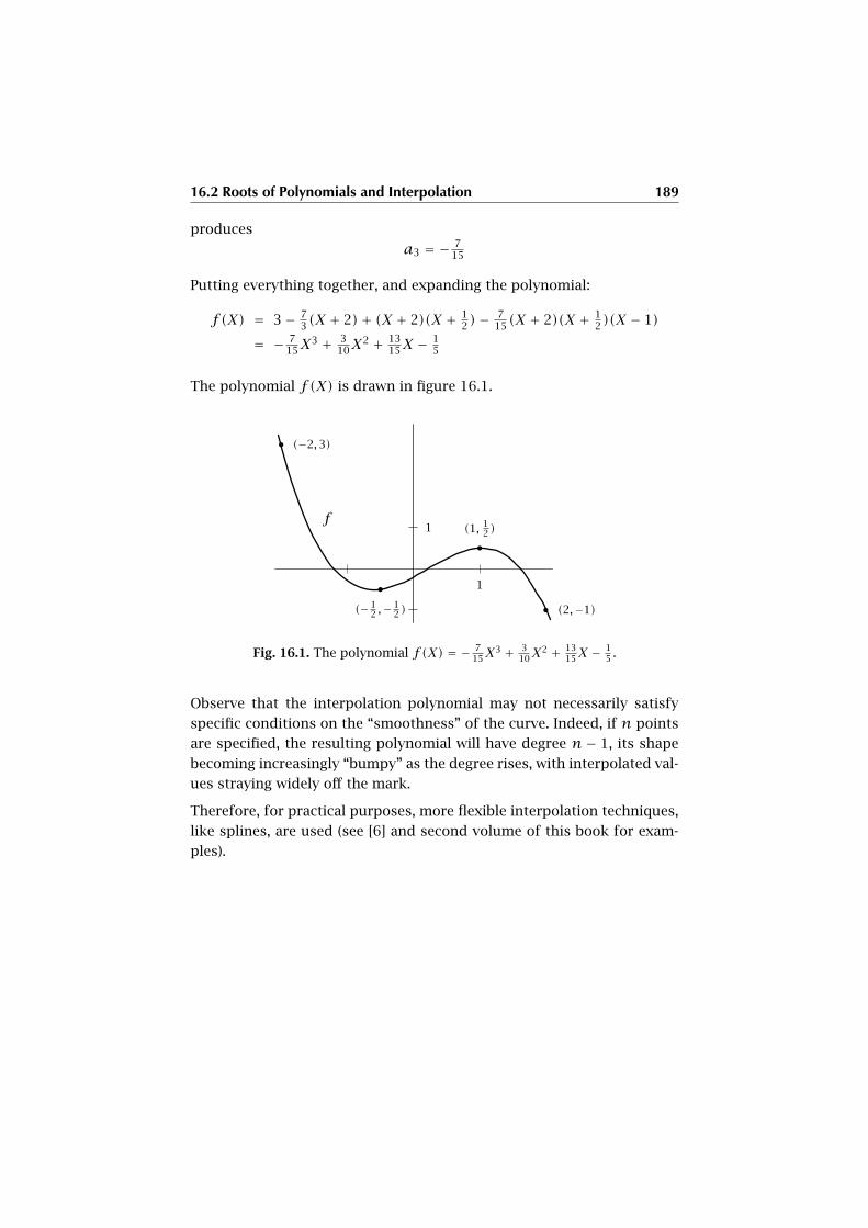
16.2 Roots of Polynomials and Interpolation 189
produces
a3 = − 715
Putting everything together, and expanding the polynomial:
f(X) = 3− 73(X + 2)+ (X + 2)(X + 1
2)− 715(X + 2)(X + 1
2)(X − 1)
= − 715X
3 + 310X
2 + 1315X − 1
5
The polynomial f(X) is drawn in figure 16.1.
1
1
(− 12 ,− 1
2 )
(−2,3)
(1, 12 )
(2,−1)
f
Fig. 16.1. The polynomial f(X) = − 715X
3 + 310X
2 + 1315X − 1
5 .
Observe that the interpolation polynomial may not necessarily satisfy
specific conditions on the “smoothness” of the curve. Indeed, if n points
are specified, the resulting polynomial will have degree n − 1, its shape
becoming increasingly “bumpy” as the degree rises, with interpolated val-
ues straying widely off the mark.
Therefore, for practical purposes, more flexible interpolation techniques,
like splines, are used (see [6] and second volume of this book for exam-
ples).
CHAPTER 17
Formal Propositional Logic
Until now, we have been using logic in its role as a guiding principle of
human thought—as such it has been described under the title of “propo-
sitional logic” in the introductory section 1.1. We are not going to replace
this fundamental human activity, but we are interested in the problem
of mimicking logical reasoning on a purely formal level. What does this
mean? The idea is that one would like to incorporate logic in the math-
ematical theory, which means that we want to simulate the process of
logical evaluation of propositions by a mathematical setup. Essentially,
this encompasses three tasks:
1. The first task is to give a mathematical construction which describes
the way in which logically reasonable propositions should be built.
For example, as we have learned from section 1.1, if A,B are propo-
sitions, one may want to build “NOTA”, “A IMPLIES B”, and so forth.
But the construction should not deal with contents, it should just
describe the combinatorial way a new expression is constructed. In
other words, this is a problem of syntax (relating to how expressions
of a sign system are combined independent of their specific meaning).
The question addressed by the first task is: How can such a syntacti-
cal building scheme be described? This task is evidently required if we
want to delegate some logical work to machines such as computers,
where content cannot be achieved without a very precise and mechan-
ical control of form.
2. Suppose that the first task of formalization has been achieved. One
then needs to rebuild the truth values which propositions should ex-
192 Formal Propositional Logic
press. This refers to the meaning or semantics of such propositions.
This is a radical point of view: The meaning of a proposition is not its
specific contents, but one of the two truth values: “true” or “false”, or,
equivalently, “is the case” or “is not the case”. For example, the mean-
ing of the proposition “if it is raining, then I am tired” has nothing to
do with rain or fatigue, it is only the truth value of the implication.
It is this semantical issue which is mimicked by the formal theory of
propositional logic. So one needs a domain of truth values, which is
addressed by a formal propositional expression in order to evaluate
its ‘meaning’. Such domains will be called logical algebras. Therefore,
the second task is to give a rigorous mathematical description of what
a logical algebra is which manages the semantic issue of propositional
logic.
3. The third task deals with the connection of the first two tasks, i.e.,
given a syntactical description of how to build correct propositions,
as well as a logical algebra which manages the semantics of truth val-
ues, we need to specify how these two levels are related to each other.
This third task is that of “signification”, i.e., the mathematically rigor-
ous definition of an association of meaning with a given propositional
expression.
We should, however, pay attention to the power of such a formalization
procedure, since often a naive understanding thereof claims to be a re-
placement of our human reasoning and its contents by purely formal de-
vices. There is a fundamental error, which is easily explained: A formal,
i.e., mathematical theory of propositional logic as sketched above, must
rely on given mathematical structures and results, the most important
one being set theory, the theory of natural numbers, and—above all—the
recursion theorem, which is a fundamental tool for the construction of
formal expressions and for the proof of properties which are shared by
formal expressions. In order to keep the level of human thought and the
formal logical level separate, we never use symbols of formal logic in for-
mulas which are meant as a human thought. In a famous 1931 paper On
Formally Undecidable Propositions of Principia Mathematica and Related
Systems, the mathematician Kurt Gödel demonstrated that within any
given branch of mathematics, there would always be some propositions
that could not be proved either true or false using the rules and axioms
of that mathematical branch itself. Gödel himself alluded to machine-
supported logical reasoning. But subsequently, many philosophers, the-
17.1 Syntactics: The Language of Formal Propositional Logic 193
ologists and would-be scientists concluded that human thought, as well,
is tainted by these incompleteness properties, actually derived for formal
systems only. We hope that the reader may understand in the following
that these formalizations of human thought are just low-level simulations
of its mechanical flattening, and not of proper thought. An example will
be presented arguing that there are propositions which are undecidable
in a given formal system, but can be decided using unformalized thought.
17.1 Syntactics: The Language of Formal
Propositional Logic
The language of formal propositional logic aims to create the variety of
possible propositions. The concept of proposition is elementary. There-
fore, the only possibility to build new propositions is to start with given
ones and to combine them by logical operations. Here is the formal setup
of the repertory of expressions with which we shall work in order to build
logically reasonable propositions:
Definition 108 A propositional alphabet is a triple A = (V , B, C) of mutu-
ally disjoint sets, where
(i) the set V is supposed to be denumerable, i.e., equipollent to N, and
the elements v0, v1, . . . ∈ V are called propositional variables;
(ii) the set B = {(,)} of (, the left bracket and ), the right bracket;
(iii) the set C = {!, &, |, −> } consists of these four logical connective
symbols, the negation symbol !, the conjunction symbol &, the dis-
junction symbol |, and the implication symbol −> .
The monoid EX = EX (A) = Word(V t B t C) is called the monoid of
expressions over A. Within EX , the subset S(EX ) of sentences over A is
the smallest subset S(EX ) ⊂ EX with the following properties:
(i) V ⊂ S(EX );
(ii) if α ∈ S(EX ), then (!α) ∈ S(EX );
(iii) if α,β ∈ S(EX ), then (α & β) ∈ S(EX );
(iv) if α,β ∈ S(EX ), then (α | β) ∈ S(EX );
(v) if α,β ∈ S(EX ), then (α −> β) ∈ S(EX ).
The set S(EX ) is also called the propositional language defined by A.
194 Formal Propositional Logic
Observe that the symbols of A have been chosen for the sake of the log-
ical context, but strictly speaking, they are simply sets with no special
properties whatsoever.
As it is defined, the language S(EX (A)) is not effectively described—
we can only tell that, for example, expressions such as v0, (!v3), and
(v2 & v6) are sentences. But there is no general control of what is possi-
ble and what is not.
Exercise 72 Show that the expression !(!v1) is not a sentence.
Is (v3 −> (!v2)) a sentence?
We now give a recursive construction of the subset S(EX ) ⊂ EX for a
given alphabet A. To this end, we use the fact that we have the union of
disjoint sets S(EX ) = ⋃n≥0 Sn(EX ), where Sn(EX ) = S(EX ) ∩ EXn, with
EXn = {w ∈ EX | l(w) = n} the set of expressions of word length n.
Here is the structure of S(EX ) given in these terms:
Definition 109 Given a propositional alphabet A, let Sn be the following
subsets of EXn, which we define by recursion on n:
(i) For n = 0,2,3, we set Sn = ∅;
(ii) we set S1 = V ;
(iii) we set S4 = {(!vi) | vi ∈ V};(iv) we set S5 to the set of words of one of these three types: (vi & vj),
(vi | vj), (vi −> vj), where vi, vj ∈ V are any two propositional
variables;
(v) for n > 5, we set Sn = S !n ∪ S&
n ∪ S|n ∪ S −>n , where S∗n = {(α ∗ β) |α,β ∈ ⋃i<n Si, l(α)+ l(β) = n− 3} for the symbols ∗ ∈ {&, |, −> },and where S !
n = {(!α) | α ∈ Sn−3}.
We then set S = ⋃n≥0 Sn.
Example 71 To illustrate the construction of the sets Si, we give them
for the set of variables V = {v} up to S8. The sets grow quickly with
increasing i even with only one variable. The reader should check that
the sets conform to the rules of definition 109, in particular that each Sionly contains expressions of exacty length i.

17.1 Syntactics: The Language of Formal Propositional Logic 195
S0 = {},S1 = {v},S2 = {},S3 = {},S4 = {(!v)}S5 = {(v & v), (v | v), (v −> v)}S6 = {}S7 = {(!(!v))}S8 = {(v & (!v)), ((!v) & v),
(v | (!v)), ((!v) | v),(v −> (!v)), ((!v) −> v),(!(v & v)), (!(v | v)), (!(v −> v))}
Proposition 144 Given a propositional alphabet A, we have
S(EX ) = S,
where S is the set defined in definition 109.
Proof Clearly, S is contained in S(EX ). Let us check that it fulfills the five axioms
(i) through (v). By construction, V = S1, whence (i). If α ∈ S, then for l(α) ≤ 3,
we only have α ∈ V , and S4 covers the case (!α) ∈ S, else l(α) > 3, and this case
is covered by construction v of the definition of S, whence (ii). The cases (iii)–(v)
are similar: for l(α)+ l(β) ≤ 3, we must have α,β ∈ V , this is covered by (iv) in
the definition of S. For l(α)+ l(β) > 3, construction (v) in the definition does the
job. �
We now know how the construction of the sentences over A works, but
we still do not know how many sentences α and β could give rise to one
and the same sentence, say w = (α & β).
Lemma 145 If left(w) and right(w) denote the numbers of left and right
brackets, respectively, in a sentence w ∈ S(EX ), then we have left(w) =right(w).
Proof The construction of S(EX ) by S guaranteed by proposition 144 yields a
straightforward inductive proof by the length of a sentence. �
Exercise 73 Give a proof of lemma 145 by recursion on the length of w.
196 Formal Propositional Logic
Lemma 146 Let w ∈ S(EX ), and suppose that we have a left bracket ( in
w, i.e., w = u(x, with l(u) > 0. Then if the number of left brackets in (x
is l and the number of right brackets in (x is r , we have l < r .
Proof Induction on l(w): For l(w) ≤ 5, it is clear by the explicit words from
rules (i)–(iv) in the definition of S. For general w, if w = u(x = (!α), then u = (!
or u = (!u′, where u′(v′ = α. By induction, the number of left brackets in (v ′
is smaller than the number of right brackets. So the same is true for (x = (v ′).
A similar argument is used for the other connectives. �
Proposition 147 Letw ∈ S(EX ). Then exactly one of the following decom-
positions is the case: w ∈ V , or w = (!α), or w = (α & β), or w = (α | β),or w = (α −> β), where α and β are uniquely determined sentences. They
are called the components of w.
Proof First, suppose (!α) = (!α′), then clearly the inner words α and α′ must be
equal. Second, suppose (!α) = (β ∗ γ), then the letter ! must be the first letter
of β, which is impossible for any sentence. Then suppose (α ∗ β) = (γ ∗ δ). If
l(α) = l(γ), then α = γ, therefore also β = δ. So suppose wlog (without loss of
generality) l(α) < l(γ). Then β = (γ′∗δ, where γ = x(γ′. So by lemma 146, (γ′
has fewer left than right brackets. But this contradicts the fact that β and δ have
the same number of left and right brackets. �
This proposition has deep implications. In fact, it allows the definition of
functions on S(EX ) by recursion on the length of sentences and and in
function of the unique logical connectives defining compound sentences.
But let us first discuss the announced “logical algebras”.
17.2 Semantics: Logical Algebras
On the syntactic level of a formal propositional language S(EX ) over a
propositional alphabetA, the sentences look like meaningful expressions.
However, they really only look meaningful. In order to load such expres-
sions with logical meaning, we need to provide the system with logical
values. In order to have a first orientation of what a logical algebra should
be, we refer to the “Boolean algebra” of subsets L = 2a of a set a as dis-
cussed in chapter 3, and especially in proposition 7. More specifically, in
the special case of a = 1 = {0}, we have two subsets, ⊥ = ∅ = 0 and
> = 1. Following a classical idea of the great mathematician and philoso-
pher Gottfried Wilhelm Leibniz (1646–1716) and its elaboration by the
mathematician George Boole (1815–1864), one can mimic truth values on

17.2 Semantics: Logical Algebras 197
the Boolean algebra L = 2 = 21 as described in proposition 7. The value
“true” is represented by >, whereas the value “false” is represented by ⊥.
The truth table of the conjunction A AND B is given by the Boolean op-
eration of intersection of the truth values assigned to the components,
i.e., if A is true and B is false, the truth value of the conjunction is
> ∩ ⊥ = ⊥, and so on with all other combinations. In other words, we
are combining the values value(A), value(B) ∈ 2 under Boolean oper-
ations. We see immediately that the Boolean operation “∩” stands for
conjunction, “∪” for disjunction, and complementation “−” for negation,
whereas the truth value ofA IMPLIES B is the value of (NOTA) OR B, i.e.,
(−value(A))∪ value(B). However, it is not always reasonable to deduce
logical implication from negation and disjunction, we rather would like
to leave this operation as an autonomous operation. This is very impor-
tant in order to cope with non-classical logical approaches, such as fuzzy
logic. This approach was formalized by the mathematician Arend Heyting
(1898–1980):
Definition 110 A Heyting algebra (HA) is a partially ordered set (L,≤),together with
• three binary operations: the join a∨ b, the meet a∧ b, and the impli-
cation a⇒ b for a,b ∈ L, and
• two distinguished elements ⊥ and >, called “False” and “True”, respec-
tively.
These data are subjected to the following properties:
(i) ⊥ and > are the minimal and maximal element with respect to the
given partial ordering, i.e., ⊥ ≤ x ≤ > for all x ∈ L.
(ii) The operations join and meet are commutative.
(iii) Join and meet are mutually distributive, i.e., x∧(y∨z) = (x∧y)∨(x ∧ z) and x ∨ (y ∧ z) = (x ∨y)∧ (x ∨ z), for all x,y, z ∈ L.
(iv) The join x ∨y is a least upper bound (l.u.b) of x and y , i.e., x,y ≤x ∨y and for any z with x,y ≤ z, we have x ∨y ≤ z.
(v) The meet x ∧ y is a greatest lower bound (g.l.b.) of x and y , i.e.,
x ∧y ≤ x,y and for any z with z ≤ x,y , we have z ≤ x ∧y .
(vi) (Adjunction) For any z ∈ L, z ≤ (x ⇒ y) iff z ∧ x ≤ y .
For an element x of a Heyting algebra L, we define the negation of x by
¬x = (x ⇒ ⊥).

198 Formal Propositional Logic
Exercise 74 Show that in a Heyting algebra, we always have y ≤ ¬x iff
y ∧ x = ⊥. Deduce from this that always
¬x ∧ x = ⊥.
Use the adjunction characterization (vi) of definition 110 to prove that
((x ∨y)⇒ z) = ((x ⇒ z)∧ (y ⇒ z)).
More specifically, prove De Morgan’s first law:
¬(x ∨y) = ¬x ∧¬y.
Definition 111 In a Heyting algebra L, a complement of an element x is
an element a such that x ∧ a = ⊥ and x ∨ a = >.
Lemma 148 The complement of an element x in a Heyting algebra L, if it
exists, is uniquely determined.
Proof If b is another complement of x, we have b = b ∧ > = b ∧ (x ∨ a) =(b ∧ x)∨ (b ∧ a) = (x ∧ a)∨ (b ∧ a) = (x ∨ b)∧ a = >∧ a = a. �
Exercise 75 Show that y ≤ ¬xa y ∧ x = ⊥.
An important and classical type of special Heyting algebras is defined by
these properties:
Lemma 149 For a Heyting algebra L, the following properties are equiva-
lent: For all x ∈ L,
(i) x ∨¬x = >,
(ii) we have ¬¬x = x.
Proof Observe that always ¬> = ⊥ and ¬⊥ = >.
(i) implies (ii): If x ∨ ¬x = >, then by De Morgan’s first law (exercise 74), ¬x ∧¬¬x = ⊥. So ¬¬x is a complement of ¬x, but x is also a complement of ¬x,
therefore, by uniqueness of complements (lemma 148), ¬¬x = x.
Conversely, if ¬¬x = x, then by De Morgan’s first law, x∨¬x = ¬(¬x∧¬¬x) =¬(¬x ∧ x) = ¬⊥ = >. �
Definition 112 A Heyting algebra which has the equivalent properties of
lemma 149 is called a Boolean algebra (BA).
17.2 Semantics: Logical Algebras 199
Example 72 The classical example is the “Boolean algebra” of subsets
L = 2a of a given set a, as discussed in chapter 3. Here, the partial or-
dering is the set inclusion, i.e., x ≤ y iff x ⊂ y . We define −x = a − x,
and have ⊥ = ∅,> = a, ∨ = ∪,∧ = ∩, and x ⇒ y = −x ∪ y . Evi-
dently, ¬x = (−x)∪∅ = −x, whence x ⇒ y = (¬x)∨y , i.e., implication
is deduced from the other operations. It is really a BA since the double
complementation is the identity: −(−(x)) = x. This is the a posteriori
justification for the name “Boolean algebra”, which we attributed to the
powerset algebra in chapter 3. But observe that for a general set a, many
truth values are possible besides the classical ⊥ and >.
Example 73 A less classic example is the set L = Fuzzy(0,1) of all inter-
vals Ix = [0, x[⊂ [0,1[ of the “half open” real unit interval [0,1[= {x |0 ≤ x < 1} ⊂ R. Its elements are so-called fuzzy truth values, meaning
that something may be true to x · 100%, i.e., not entirely true, and not
entirely false. The percentage is given by the upper number x of the in-
terval Ix . The partial ordering is again that of subset inclusion, and the
extremal values are ⊥ = I0 = ∅ and > = I1. We also take ∨ = ∪ and
∧ = ∩. This means Ix ∨ Iy = Imax(x,y) and Ix ∧ Iy = Imin(x,y).
The implication is a little more tricky. We must have Iz ≤ (Ix ⇒ Iy) iff
Iz ∩ Ix ⊂ Iy . The solution therefore must be Ix ⇒ Iy =⋃z,Iz∩Ix⊂Iy Iz.
Therefore Ix ⇒ Iy = Iw , with w = sup{z | Iz ∩ Ix ⊂ Iy}. This gives the
following implications: Ix ⇒ Iy = > if x ≤ y , and Ix ⇒ Iy = Iy if x > y .
In particular, ¬Ix = ⊥ if x ≠ 0, ¬⊥ = >. And finally, ¬¬Ix = > if x ≠ 0,
¬¬⊥ = ⊥. This also shows that this Heyting algebra Fuzzy(0,1) is not
Boolean. For the general theory of fuzzy systems, see [34] or [48].
We shall henceforth use the term logical algebra for a Heyting algebra or,
more specifically, for a Boolean algebra. Intuitively, a logical algebra is a
structure which provides us with those operations “negation”, “conjunc-
tion”, “disjunction”, and “implication” which are defined by the formal
logical setup and should simulate the “reality of logical contents”.
Here are the general properties of logical algebras:
Sorite 150 Let L be a Heyting algebra and x,y ∈ L. Then
(i) x ≤ ¬¬x,
(ii) x ≤ y implies ¬y ≤ ¬x,
(iii) ¬x = ¬¬¬x,
200 Formal Propositional Logic
(iv) (De Morgan’s first law) ¬(x ∨y) = ¬x ∧¬y .
(v) ¬¬(x ∧y) = ¬¬x ∧¬¬y ,
(vi) x ∧y = ⊥ iff y ≤ ¬x,
(vii) x ∧¬x = ⊥,
(viii) (x ⇒ x) = >,
(ix) x ∧ (x ⇒ y) = x ∧y ,
(x) y ∧ (x ⇒ y) = y ,
(xi) x ⇒ (y ∧ z) = (x ⇒ y)∧ (x ⇒ z).In particular, if L is a Boolean algebra, then
(xii) x = ¬¬x,
(xiii) x ∨¬x = >,
(xiv) x ⇒ y = ¬x ∨y ,
(xv) x ≤ y iff ¬y ≤ ¬x,
(xvi) (De Morgan’s second law) ¬(x ∧y) = ¬x ∨¬y .
Proof By exercise 74, x ≤ ¬¬x iff x ∧ ¬x = ⊥, but the latter is always true. If
x ≤ y , then also x ∧¬y ≤ y ∧¬y = ⊥, so ¬y ∧ x = ⊥, therefore ¬y ≤ ¬x.
Statement (iii) follows immediately from (i) and (ii).
(iv) is De Morgan’s first law (see exercise 74).
The proof of (v) is quite technical and is omitted, see [36].
Statements (vi) and (vii) follow from exercise 74.
Statements (viii) to (xi) immediately follow from the characterization of the g.l.b.
and adjointness for implication.
(xii) and (xiii) is the characterization from lemma 149.
For (xiv), we show z ≤ (¬x ∨ y) iff z ∧ x ≤ y . If z ∧ x ≤ y , then z = z ∧ 1 =z ∧ (¬x ∨ x) = (z ∧¬x)∨ (z ∧ x) ≤ ¬x ∨ y . Conversely, if z ≤ (¬x ∨ y), then
z ∧y ≤ (¬x ∨y)∧y ≤ (¬x ∧y)∨ (y ∧y) ≤ (¬x ∧y)∨y .
(xv) follows from (ii) and (xii). �
17.3 Signification: Valuations
We may now turn to the third component of a semiotic (sign-theoretic)
system: the signification process from the expressive surface down to
the semantic depth. Our modeling of such a system by use of a proposi-
tional alphabet A and a logical algebra L must provide us with a function
17.3 Signification: Valuations 201
value : S(EX ) → L such that each sentence w ∈ S(EX ) is assigned a truth
value value(w) ∈ L. Such a valuation should however keep track with the
requirement that logical evaluation is related to the logical composition
of these sentences. Here is the precise setup:
Definition 113 Given a propositional alphabet A and a logical algebra
L, a valuation is a map value : S(EX ) → L such that for all sentences
α,β ∈ S(EX ), we have
(i) value((!α)) = ¬(value(α)),
(ii) value((α | β)) = value(α)∨ value(β),
(iii) value((α & β)) = value(α)∧ value(β),
(iv) value((α −> β)) = value(α)⇒ value(β).
The set of valuations value : S(EX ) → L over the propositional alphabet A
with values in the logical algebra L is denoted by V (A, L).
And here is the existence theorem for valuations:
Proposition 151 Given a propositional alphabet A, a set of variables V
and a logical algebra L, the functional restriction map
var : V (A, L)→ Set(V , L) : value , value|Vis a bijection, i.e., for each set map v : V → L defined on the propositional
variables, there is exists exactly one valuation value : S(EX ) → L such that
value|V = v . In other words, once we know the values of the variables, we
know the values of all expressions.
Proof Injectivity is proved by induction on the length of a sentence w. For
length 1, we have values from V , and this is what we want. For l(w) > 1, we have
one of the formsw = (!α), (α | β), (α & β), (α −> β), and the induction hypothe-
sis on α,β, together with the axiomatic properties (i)–(iv) of valuations solve the
problem. Conversely, if a map vV : V → L is given, its extension to any sentence
w ∈ S(EX) may be defined by recursion following the axiomatic properties (i)–
(iv) of valuations. This is indeed well defined, because by proposition 147, the
form and the components of a compound sentence are uniquely determined by
w. �
Exercise 76 Given a propositional alphabet A, let a = 3 = {0,1,2} and
consider the powerset Boolean algebra L = 23. Let a value map value ∈V(A, L) be defined by value(v0) = ⊥, value(v1) = {0,2}, value(v2) ={1}, . . . . Calculate the value
202 Formal Propositional Logic
value(((!(v2 & (!v0))) | ((!v1) −> v2))).
Notation 11 For long expressions, such as the still rather short example
in the previous exercise 76, the number of brackets becomes cumbersome
to keep under control. To avoid this effect, one uses the same trick as for
ordinary arithmetic: strength of binding, i.e., the formal rules are replaced
by some implicit bracket constructions which enable us to omit brackets in
the notation. The rules of binding strength are these: ! binds stronger than
& and |, and these bind stronger than −> . Under this system of rules, the
above example
((!(v2 & (!v0))) | ((!v1) −> v2))
would be shortened to
!(v2 & !v0) | (!v1 −> v2)
The main problem of formal propositional logic is to understand which
kind of sentences w ∈ S(EX ) have the value value(w) = > under cer-
tain valuations. The most prominent of these questions is the problem
of so-called tautologies, i.e., sentences, which have the value > under all
possible valuations of a given class. Here is the formalism:
Definition 114 Given a propositional alphabet A, a logical algebra L, a
sentence s ∈ S(EX ), and a valuation v ∈ V(A, L), one says that s is v-
valid if v(s) = >, in signs: v î s. If v î s for all v ∈ V(A, L), one says
that s is L-valid, in signs L î s. In particular, if 2 î s, one says that s is
classically valid or that s is a tautology and writes î s. If s is valid for all
Boolean algebras, one says that s is Boolean valid and writes BA î s. If s is
valid for all Heyting algebras, one says that s is Heyting valid and writes
HA î s.
Exercise 77 Show that for any sentence s ∈ S(EX ), we have HA îs −> !!s and BA î !!s −> s. Give an example of a HA L such that
L î !!s −> s is false.
In order to control what kinds of sentences are valid for given valuation
classes, one needs a more constructive approach, such as the axiomatic
method.
17.4 Axiomatics 203
17.4 Axiomatics
Axiomatics is about the construction of a set of new sentences from given
ones by use of a predetermined system of inference rules. This setup is a
particular case of so-called production grammars, which will be discussed
in chapter 19. Here, we stay rather intuitive as to the general nature of
such an inference rule system and will only concentrate on a special type,
the one defined by the classical inference rule modus ponens (the Latin
name is a marker for the Medieval tradition of formal logic). It is the
rule which we apply constantly: If A is the case (i.e., true), and if the
implication A IMPLIES B is the case, then also B is the case. In fact,
otherwise, by absolute logic, B would not be the case (false), but then AIMPLIES B cannot be the case by the very definition of implication. The
formal restatement of this inference rule defines classical axiomatics as
follows.
Definition 115 One is given a set AX ⊂ S(EX ) of sentences, called axioms.
A proof sequence (with respect to AX ) is a finite sequence p = (si)i=1,2...n ∈S(EX )n of positive length l(p) = n such that s1 ∈ AX , and for i > 1, either
si ∈ AX , or there are two sentences sk and sl = (sk −> si) where k, l < i.
A terminal sentence sn in a proof chain is called a theorem with respect
to AX . The set of theorems is denoted by SAX (EX ). If SAX (EX ) is clear, the
fact that s ∈ SAX (EX ) is also denoted by |——AXs.
Intuitively, the role of axioms is this: One accepts axioms as being true a
priori, i.e., one only looks for classes of valuations which map all axioms
to >. One then wants to look for all sentences which are also true if the
axioms are so. The only rule is the formalized modus ponens: Given two
theorems s and (s −> t), then t is also a theorem. Evidently, this pro-
cess can be managed by a machine. The point of axiomatics is that proof
sequences starting from a particular set of axioms yield the tautologies.
Definition 116 The axioms of classical logic (CL) are the sentences which
can be built from any given three sentences α,β, γ ∈ S(EX ) by one of the
following constructions:
(i) (α −> (α & α))
(ii) ((α & β) −> (β & α))
(iii) ((α −> β) −> ((α & γ) −> (β & γ)))
204 Formal Propositional Logic
(iv) (((α −> β) & (β −> γ)) −> (α −> γ))(v) (β −> (α −> β))
(vi) ((α & (α −> β)) −> β)(vii) (α −> (α | β))
(viii) ((α | β) −> (β | α))(ix) (((α −> β) & (β −> γ)) −> ((α | β) −> γ))(x) ((!α) −> (α −> β))
(xi) (((α −> β) & (α −> (!β))) −> (!α))(xii) (α | (!α))
The axioms of intuitionistic logic (IL) are those sentences in CL built from
all constructions except for the last, (α | (!α)).
The intuitionistic axiom system IL contains those axioms which we need
to produce sentences which are Heyting valid. Recall that we have in fact
Heyting algebras L, for example L = Fuzzy(0,1), where x ∨ (¬x) ≠ > in
general. The crucial proposition is this:
Proposition 152 Given a propositional alphabet A and a sentence s ∈S(EX ), the following statements are equivalent:
For classical logic:
(i) The sentence s is a tautology, i.e., î s.(ii) The sentence s is Boolean valid, i.e., BA î s.
(iii) s is a theorem with respect to CL, i.e., |——CLs
And for intuitionistic logic:
(i) The sentence s is Heyting valid, i.e., HA î s.(ii) s is a theorem with respect to IL, i.e., |——
ILs
Proof (ii) implies (i): This is similar to proposition 153 which deals with (iii)
implies (i), i.e., the special case where BA is the set 2.
(i) implies (iii): This part is proposition 154.
The equivalence of (i) and (ii) in the intuitionistic case follows these lines: Sound-
ness, i.e., (i) implies (ii) follows as easily as soundness for Boolean algebras. Com-
pleteness is proved as follows: From |——ILs, one constructs a special Heyting al-
gebra, the so-called Lindenbaum algebra HIL. Then one shows that the validity
for this algebra implies |——ILs. So finally, as HA î s implies HIL î s, we are
17.4 Axiomatics 205
done. The details are beyond the scope of this introductory book, but see [38]
for details. �
The equivalence of (i) and (iii) of the Boolean part of this theorem is of
particular significance. Historically, each direction has been introduced
as a distinct theorem. We now state both theorems separately.
The first theorem, corresponding to the direction from (iii) to one deals
with the requirement that only tautologies can be proved from the axiom
system CL of classical logic, only tautologies are generated. This is the
so-called soundness theorem:
Proposition 153 (Soundness) If |——CLs, then î s.
This is just an exercise:
Exercise 78 Prove proposition 153 as follows: First show that all axioms
are classically valid. Then show by induction on the proof chain length
that any theorem is classically valid.
The more involved part is the converse, the so-called completeness theo-
rem:
Proposition 154 (Completeness) If î s, then |——CLs.
We shall not give a proof of the completeness theorem, which is quite
involved. The original proof of such a theorem was given in 1921 by Emil
Post (see [45]).
Example 74 The sentences (α −> (β | α)) for α,β ∈ S(EX ) seem to
be obvious theorems of CL, especially since (α −> (α | β)) is an axiom
schema. But we have to provide a proper proof sequence in order to estab-
lish this fact. On the right of each line of the proof sequence we indicate
whether we have used an axiom (ax.) or applied modus ponens (m.p.) to
two of the previous lines. Circled numbers À and Á are used as abbrevi-
ations to refer to the formulas in line 1 and line 2, respectively. (To be
absolutely accurate, we should state that the following proof sequence is
really a schema for generating proof sequences of (α −> (β | α)) for all
α,β ∈ S(EX )).

206 Formal Propositional Logic
1. (α −> (α | β)) ax. (vii)
2. ((α | β) −> (β | α)) ax. (viii)
3. (À −> (Á −> À)) ax. (v)
4. (Á −> À) m.p. 1, 3
5. ((Á −> À) −> ((Á & Á) −> (À & Á))) ax. (iii)
6. ((Á & Á) −> (À & Á)) m.p. 4, 5
7. (Á −> (Á & Á)) ax. (i)
8. (Á & Á) m.p. 2, 7
9. (À & Á) m.p. 6, 8
10. (((α −> (α | β)) & ((α | β) −> (β | α))) −> (α −> (β | α))) ax. (iv)
11. (α −> (β | α)) m.p. 9, 10
Hence |——CL(α −> (β | α)) for all α,β ∈ S(EX ).
This proof was rather easy and short. However, proof sequences for the-
orems of even a little more complexity tend to become long and intricate.
Therefore, whenever one has established the theoremhood of a sentence,
one may use it in subsequent proof sequences just as if it were an axiom.
If asked, one could then always recursively expand the theorems to their
proof sequences to get a sequence in the originally required form.
Sorite 155 Abbreviating ((α −> β) & (β −> α)) by (α <−> β), the follow-
ing sentences are tautologies:
1. (Associativity)
((α | β) | γ <−> α | (β | γ)) and ((α & β) & γ <−> α & (β & γ))
2. (Commutativity) (α | β <−> β | α) and (α & β <−> β & α)
3. (De Morgan’s Laws)
((!(α | β)) <−> (!α & !β)) and ((!(α & β)) <−> (!α | !β))
Proof The sentences can be proved along the lines of example 74. However the
proofs quickly become very unwieldy, and to handle them at all, a number of
tools have to be developed, such as the Deduction Theorem. For more details
about proof theory, see any book on mathematical logic, such as [17]. �
One also calls sentences s and t equivalent iff (s <−> t) is a tautology.
Notice that from the associativity, we may group conjunctions or disjunc-
tions in any admissible way and obtain sentences which are equivalent to
each other. We therefore also omit brackets in multiple conjunctions or
disjunctions, respectively.
17.4 Axiomatics 207
Exercise 79 A sentence s is in disjunctive normal form iff s = s1|s2| . . . sk,where each si is of the form si = si1 & si2 & . . . sik(i) with sij being a
propositional variable v ∈ V or its negation (!v).
A sentence s is in conjunctive normal form iff s = s1 & s2 & . . . sk, where
each si is of the form si = si1 | si2 | . . . sik(i) with sij being a propositional
variable v ∈ V or its negation (!v).
Use the axioms and the sorite 155 to show that every sentence is equiv-
alent to a sentence in disjunctive normal form and also to a sentence in
conjunctive normal form.
Exercise 80 Define the Sheffer stroke operator by (α || β) = (!(α & β)).
Show that every sentence is equivalent to a sentence, where only the Shef-
fer operator occurs. In electrical engineering the stroke operator is also
known as NAND.
CHAPTER 18
Formal Predicate Logic
Up to now, we have succeeded in formalizing basic logic as controlled by
truth values produced by the propositional connectives !,&, |, and −>of negation, conjunction, disjunction, and implication. However, nothing
has been done to mimic the ‘anatomy of propositions’, in fact, we had
just offered an ‘amorphous’ set of propositional variables v0, v1, . . . with
no further differentiation. So the truth value of sentences was based on
the completely arbitrary valuation of propositional variables.
Now, mathematics needs more refined descriptions of how truth and
falsity are generated. For example, the simple set-theoretic definition
a ∩ b = {x | x ∈ a and x ∈ b} uses composed predicates: (1) P(x)
is true iff x ∈ a, (2) Q(x) is true iff x ∈ b, and the combination thereof
(P & Q)(x) is true iff P(x) andQ(x) are both true. So, first of all we need
to formalize the concept of a predicate.
Next, let us look at the pair axiom: “If a and b are two sets, then there is
the pair set {a,b}.” This statement uses the predicates (1) S(x) is true iff
x is a set, (2) E(x,y) is true iff both S(x) and S(y) are true, and x ∈ y .
We implicitly also need the predicate I(x,y) which is true iff both S(x)
and S(y) are true, and x = y . This setup transforms the axiom to the
shape “If a and b are such that S(a) and S(b), then there is c with E(a, c)
and E(b, c), and if x is such that E(x, c), then I(x,a) or I(x, b).” Besides
the predicative formalization, we here encounter two more specifications:
the first part “If a and b are such that S(a) and S(b). . . ”, which means
“Whenever we take a, b. . . ”, in other words, we suppose a given universe
of objects from where we may select instances a and b and then ask them
to comply with certain predicates S(a) and S(b), i.e., to be sets. This is

210 Formal Predicate Logic
expressed by the so-called universal quantifier : “For all a, b. . . ”. Further,
we also recognize an existence quantifier : “. . . there is c with . . . ”, which
is expressed by “. . . there exists c with . . . ”.
In order to cope with the common mathematical constructions, one usu-
ally is a bit more specific in the formalization of predicates. As modeled
from set theory, there are two basic types of predicates: relations and
functions. This means that we are considering predicates defined by re-
lations and functions in the following sense: Given n sets A1, . . . An and
an n-ary relation, i.e., a subset R ⊂ A1× . . . An of their Cartesian product,
one defines the associated n-ary predicate by R(x1, . . . xn) which is true
iff (x1, . . . xn) ∈ R. Observe that n-ary relations generalize the more re-
strictive concept of an n-ary relation R ⊂ an introduced in definition 33
by varying each of the n factors of an. Similarly, if f : A1× . . . An → An+1
is a set function, one defines the predicate f(x1, . . . xn, y) which is true
iff f(x1, . . . xn) = y . This includes the two special cases where n = 0. For
0-ary relations, this means that we consider the ‘empty Cartesian prod-
uct’ (check the universal property of Cartesian products to understand
the following definition). We are given a subset of the final set 1, in other
words, one of the classical truth values ⊥,> of the Boolean algebra 2.
Thus, we also include the extremal truth values as basic predicates. As to
functions of 0 variables, this means that the domain is again the empty
Cartesian product 1. So a 0-ary function f : 1 → A1 is identified with
the image y = f(0) of the unique argument 0 ∈ 1, in other words, 0-ary
functions are just ‘constant’ elements in A1.
A last remark must be made concerning variables. We have constantly
used some symbols a,b,x, etc. to feed the predicates. The nature of
these variables has not been discussed. Since predicates are generated
by relations or functions, we may interpret variables to refer to values in
the corresponding domain sets Ai. However, variables may not refer to
relations or functions or even higher order objects, such as relations of
relations, etc. Together with this last restriction we have what is called
first order (formal) predicate logic.
We are now ready to set up the formal framework. The methodology is
quite the same as for formal propositional logic: One first defines the
syntactical structures, then the objects of semantics, and finally the for-
malization of signification.
18.1 Syntactics: First-order Language 211
18.1 Syntactics: First-order Language
The basis of the formalized language is again a set of alphabetic symbols
which we then combine to obtain reasonable words. Let us first formalize
the relations and functions, together with the corresponding variables.
To this end, if S is a set, define by Sequ(S) the set of finite sequences
s = (A1, . . . , An),Ai ∈ S, where for n = 0 we take by definition the unique
sequence which is defined on the empty index set 0.
Exercise 81 Show that the set Sequ(S) always exists, and that Sequ(S) =Sequ(T) iff S = T .
Definition 117 For a finite set S, a signature is a triple
Σ = (FunType : Fun→ Sequ(S),RelType : Rel → Sequ(S), (VA)A∈S)
of two set maps and a family of denumerable sets VA. In the uniquely
determined S, finite by hypothesis, the elements A ∈ S are called sorts, the
elements f ∈ Fun (in the uniquely determined set Fun) are called function
symbols, and the elements R ∈ Rel (in the uniquely determined set Rel) are
called relation symbols. One supposes that all the sets Fun,Rel, and VA are
mutually disjoint. The elements x ∈ VA are called variables of sort A. The
values of FunType(f ) and RelType(R) are called the types of f and R,
respectively. The length n ≥ 0 of the type (A1, . . . An) of a relation symbol
is called its arity; the number n ≥ 0 in the type (A1, A2, . . . An+1) of a
function symbol is called its arity; so by definition, function symbols always
have at least one sort in their type. In particular, 0-ary functions are called
constants, whereas 0-ary relations are called atomic propositions.
Given a signature Σ, a function symbol f , together with its type
(A1 . . . An, An+1), is denoted by
f : A1 . . . An → An+1,
where the last sort is denoted by A since its semantic role to be defined later
is that of a codomain, but it is a sort much as the others are. A relation
symbol R, together with its type (A1 . . . An), is denoted by
R ) A1 . . . An.
In order to denote the sort A of a variable x ∈ VA or the (n + 1)st sort A
of a function f : A1 . . . An → A one also writes x : A, or f : A, respectively.
212 Formal Predicate Logic
Since we are interested in a vocabulary of general usage, we shall more-
over suppose that the following special symbols are part of our signature:
• For each sort A, the relational equality symbolA= with RelType(
A=) =(A,A) is an element of Rel, and we usually use the infix notation (a
A=b) instead of
A= (a, b), and, if the sort A is clear, we just write a = b,
but be warned: this is by no means equality in the sense of set theory,
it is just an abbreviation ofA= and has no content whatsoever on the
present syntactical level of the theory.
• Among the atomic proposition symbols we have the falsity atom ⊥ and
the truth atom >. We shall not invent new symbols for these entities
in order to distinguish them from the synonymous entities in logical
algebras since there is no danger of confusion.
Example 75 As a prototypical example, we shall develop the predicate
logic which describes Peano’s construction of natural arithmetic, a setup,
which we have modeled on the set theory of finite ordinal numbers, and
which has been described in terms of Peano’s five axioms (see proposi-
tions 45 and 47).
For Peano’s axioms we need this repertory of symbols and operations:
• A symbol for the constant 0;
• a set of variables x,y, . . . to designate natural numbers;
• a predicate symbol of equality x = y between natural numbers x,y ;
• a function symbol for the sum x +y of two natural numbers x,y ;
• a function symbol for the product x ·y of two natural numbers x,y ;
• a function symbol for the successor x+ of a natural number x.
This requirement analysis yields the following signature: We have a single
sort (the natural numbers) A, so the set of sorts is S = {A}. Accordingly,
we have one (denumerable) set of variables VA, from which we choose the
variables x,y, . . .. To fix ideas, take the set of words VA = {x0, x1, x2, . . .}with indexes being natural numbers in their decimal representation. The
set of relation symbols is Rel = { A= ) AA,⊥ ) 0,> ) 1}, the sot of func-
tion symbols is Fun = { A+ : AA → A, A· : AA → A,+A : A → A,A
0 : 1 → A},the superscripts being added to indicate that we are only setting up
a symbol set, and not real arithmetic operations. The type maps have
18.1 Syntactics: First-order Language 213
been given by the arrow notation within Fun. This means, that actually,
FunType(A+) = (A,A,A), and FunType(
A
0) = (A), the latter being the con-
stant symbol for zero.
With these symbols, one now defines the alphabet of a predicate language
as follows:
Definition 118 A predicative alphabet is a triple P = (Σ, B, C) of these
sets:
(i) The set Σ is a signature, with the defined set S of sorts, the set Fun
of function symbols, the set Rel of relation symbols, and the family
(VA)S of sets of variables.
(ii) The set B = {(, ), , } of left and right brackets, and the comma.
(iii) The set C = {!,&, |, −> ,∀,∃} of connectives, where ∀ is called the
universal quantifier, and ∃ is called the existence quantifier.
One again supposes that the sets VA, Fun,Rel, B, C are mutually disjoint.
We again have this monoid of predicative expressions:
Definition 119 Given a predicative alphabet P as explicited in defini-
tion 118, the monoid EX = EX (P) of expressions over P is the word
monoid Word(VS t Funt Rel t B t C), with VS =⊔A∈S VA.
Like with sentences, we want to construct reasonable predicative expres-
sions, which this time we call formulas instead of sentences. The con-
struction needs an intermediate step.
Definition 120 Given a predicative alphabet P , the set Term(P), the ele-
ments of which are called terms, is defined as the (uniquely determined)
minimal subset Term(P) ⊂ EX (P) such that the following two conditions
hold. Simultaneously we add the recursive definition of the sort of a term.
(i) VS ⊂ Term(P), and a variable x ∈ VA regarded as a term has the
same sort x : A as the variable as such. Attention: the expressions
x : A and f : A are not words of Term(P) or of any other formula,
they are normal mathematical formulas.
(ii) If, for 0 ≤ n, t1 : A1, . . . tn : An are terms with the respective sort
sequence of sorts (type) A1, . . . An, and if f : (A1 . . . An) → A is a
function symbol, then the expression f(t1, . . . tn) is a term, and we
214 Formal Predicate Logic
define f(t1, . . . tn) : A. In particular, the constants f() : A are terms
(the case of n = 0); for practical reasons we also include the words
f (and the notation f : A for f() : A) together with the constants
f().
Example 76 Taking up our prototypical example 75 of Peano arithmetic,
we have these terms:
• the variables xn with their (unique) sort xn : A,
• the constant symbolA
0 : A,
• the function symbols with terms in their argument places, e.g., +A(A
0),
which we presently also abbreviate byA
1, etc., nA+ 1 for +A(
A
n) (atten-
tion: this is only an informal convention to save space, but not strictly
conforming to the definition)
• the function expressions (A
0A+A
0), (A
0A·A
0), (A
0A+A
1), ((A
0A·A
0)A+A
1), and so
forth.
Similarly to the recursive construction of sentences in definition 109 and
proposition 144, one may describe Term(P) recursively.
Exercise 82 Give a recursive definition of Term(P) in terms of its inter-
sections Term(P)n = Term(P) ∩ EX (P)n, starting from Term(P)0 = ∅and Term(P)1 = Fun0 t VS , where Fun0 = {f | f ∈ Fun, FunType(f ) =(A), i.e., 0-ary} is the set of constant symbols.
We may now define general formulas for a predicative language by induc-
tion:
Definition 121 Given a predicative alphabet P , the set F(EX ) over the
predicative alphabet P is the smallest subset F(EX ) ⊂ EX = EX (P) con-
taining all these words which are called its formulas:
(i) the relational formulas R(t1, . . . tn) for R ∈ Rel, and terms ti ∈Term(P) with ti : Ai for the type RelType(R) = (A1, . . . An), includ-
ing the 0-ary relation words R(), which we again shorten to R; this
includes in particular the equality formulas (tA= s) for terms s : A
and t : A;
(ii) the truth formula > and the falsity formula ⊥;
18.1 Syntactics: First-order Language 215
(iii) negation: if φ is a formula, then so is (!φ);
(iv) disjunction: if φ and ψ are formulas, then so is (φ | ψ);(v) conjunction: if φ and ψ are formulas, then so is (φ & ψ);
(vi) implication: if φ and ψ are formulas, then so is (φ −> ψ);(vii) universal quantification: if φ is a formula, and if x is any variable,
then (∀x)φ is a formula;
(viii) existential quantification: if φ is a formula, and if x is any variable,
then (∃x)φ is a formula.
The set F(EX ) of formulas over the predicative alphabet P is called the
predicative language defined by P .
Example 77 Continuing example 76 of Peano arithmetic, we have these
formulas: In addition to the falsity and truth formulas ⊥ and >, we have
the equality relation formulas tA= s, for terms s and t, e.g.,
A
0A= (
A
0A+
A
0). We then have the formulas obtained by logical connectives which are
recursively applied to formulas, e.g., (!⊥), (!A
0A= (
A
0A+ x7)), (> & (
A
0A=
A
0)).
Finally we have the formulas obtained from the universal quantifier, e.g.,
(∀x3)(A
0A= (x3
A+ x7)), or from the existence quantifier, e.g., (∃x1)(A
0A=
+A(x1)).
Exercise 83 Give a recursive definition of F(EX ) which is based on the
formulas of given word length n, namely, F(EX )n = F(EX ) ∩ EXn, where
EXn is the set of expression with word length n.
Within this vast vocabulary, many formulas are just meaningless ‘forms’.
For example, the formula (f (x) = 3) has no meaning if the variable
x is not specified, even if we know a priori that the sorts f : B and
3 : B coincide. However, if we prepend the existence quantifier, i.e.,
(∃x)(f(x) = 3), then the formula may become meaningful, i.e., loaded
with a semantic truth value. Therefore one is interested in defining which
variables in a formula are “bound” by a quantifier, and which are not, i.e.,
“free”. Here is the precise definition of the set Free(φ) ⊂ VS of free vari-
ables of φ. It is, however, convenient to start this definition with the set
of free variables of terms. Attention: We use the fact that the components
of compound formulas, such as (∀x)φ or (φ −> ψ), are uniquely deter-
mined. We have shown such a uniqueness theorem in proposition 147,
216 Formal Predicate Logic
and it is recommended to meditate over this fact in the present context,
too! In particular, the scope of a variable x is the uniquely determined for-
mulaφ following (∀x) or (∃x) in a formula . . . (∀x)φ . . . or . . . (∃x)φ . . .,respectively.
• Free(>) = Free(⊥) = ∅;
• for a constant term t = f(), we set Free(t) = ∅;
• for a variable x, we set Free(x) = {x};• for a term t = f(t1, . . . tn),n > 0, we set Free(t) = ⋃i Free(ti);
• if φ = R(t1, . . . tn) is a relational formula, then Free(φ) = ⋃i Free(ti),
i.e., the set of all variables appearing in the terms ti;
• we set Free((!φ)) = Free(φ);
• if σ is one of the formulas (φ | ψ), (φ & ψ), (φ −> ψ), then Free(σ) =Free(φ)∪ Free(ψ);
• we set Free((∀x)φ) = Free((∃x)φ) = Free(φ)− {x}.
The concept of free variables is quite delicate. For example, the variable x
is free in the formula ((∀x)(f(x) = g(y)) & (x = x)) because it is free in
the second formula, whereas it is not free in the first formula. Intuitively,
the role of x in these two component formulas is completely different:
In the first one, x could be replaced by any other variable of the same
sort without changing the formula’s meaning. In the second component,
we could not do so because the usage of this one changes radically if we
embed it in a larger context of formulas and variables.
Definition 122 A formula φ without free variables, i.e., Free(φ) = ∅, is
called a (predicative) sentence.
The only way to produce non-trivial sentences without free variables is to
apply quantifiers. Suppose that the set VS of variables is linearly ordered
(we know that a finite disjoint union of n denumerable sets can be linearly
ordered, for example by interpreting the jth element of the ith set, i =0,1,2 . . . n− 1, as the natural number j ·n+ i). We write this ordering as
x < y for variables x and y .
Definition 123 Given a formula φ ∈ F(EX ), let x1 < x2 < . . . xr be
the ordered sequence of the elements of Free(φ). Then we denote by

18.2 Semantics: Σ-Structures 217
(∀)φ the sentence (∀x1)(∀x2) . . . (∀xr )φ, and by (∃)φ the sentence
(∃x1)(∃x2) . . . (∃xr )φ and call these sentences the universal or existen-
tial closures, respectively, of φ.
18.2 Semantics: Σ-Structures
Semantics has to provide us with logical algebras, where the truth values
can be calculated from the formal data. Here is the framework for this
calculation. Given an alphabet, the invariant data are the sets B of brack-
ets and comma, and the set C of connectives. The set which can vary is
the signature Σ. The semantic structure is tied to the signature. We need
these objects:
Definition 124 Given a signature Σ, a (set-theoretic) Σ-structure M is de-
fined by these sets:
(i) For each sort A ∈ S, we are given a set MA.
(ii) For each n-ary relational symbol R ) A1 . . . An, we are given a sub-
set MR ⊂MA1 × . . .MAn , called a relation (recall that we had defined
a relation by a subset of the second power X2 of a set X, and a graph
as a subset of a Cartesian product X×Y of sets X and Y , the present
one is a generalization of those concepts). In particular, for atomic
propositions with n = 0, e.g., ⊥ and >, we are given the subsets of
the final set 1, i.e., the truth values ⊥ = 0 and > = 1, elements in the
Boolean algebra 2.
(iii) For each n-ary function symbol f : A1 . . . An → A, we are given a
set function Mf : MA1 × . . .MAn → MA. In particular, for n = 0 we
are given a “constant”, i.e., an element Mf ∈MA.
(iv) For each equality symbolA=, we are given the diagonal relation MA= =
∆A ⊂M2A.
We shall now be able to define truth values in the Boolean algebras of the
sets MA1 × . . .MAn and to define signification of formulas with respect to
these logical algebras.
Of course, if we would take a more general Heyting algebra on the pow-
erset of such a Cartesian product, or even on Cartesian products of di-
graphs and still more ‘exotic’ objects, we would obtain a more general
218 Formal Predicate Logic
predicate logic. This can be done in the so-called topos theory (see for ex-
ample [21]), but for our modest needs, we stick to the classical situation
of Boolean powerset algebras. This is what we mean when talking about
“set-theoretic” Σ-structures.
Example 78 Following up our prototypical example 77 of Peano arith-
metic, we may define a Σ-structure M which everybody would expect: For
the sort A, take MA = N. For ⊥ and >, we have no choice by definition, i.e.,
⊥ = 0 ⊂ 1 and > = 1 ⊂ 1. For equality, we have to take MA= = ∆N. For the
functionA+ we take the ordinary addition MA+ : N×N→ N : (x,y), x+y ,
forA· we take the ordinary multiplication MA· : N×N→ N : (x,y), x ·y ,
and for +A we take the ordinary successor M+A : N → N : x , x+. Finally,
set MA0= 0 ∈ N.
But we could also take any other structure M′, for example exchanging
addition and multiplication in the above M, i.e., M′A+= MA· and M
′A· = MA+,
and setting M′A0= 23 ∈ N.
18.3 Signification: Models
The truth values of formulas are constructed as follows.
Definition 125 Let M be a Σ-structure. If t is a term and φ is a for-
mula, and if x1 < . . . xn are their free variables with corresponding sorts
A1, . . . An, we denote by Mt and Mφ, the Cartesian product MA1 × . . .MAn ,
including the special case n = 0, where we set Mt = 1 or Mφ = 1. This set
is called the free range of t and φ.
Next, we need to define evaluation of a term for specific values under a
given Σ-structure. Let t be a term, and x ∈Mt . Then the evaluation s[x] ∈Ms at x of a term s with Free(s) ⊂ Free(t) is recursively defined by (1) the
component at position s, s[x] = xs ∈ MA if s : A is a variable of sort A;
(2) the value s[x] = Mf (t1[x], . . . tm[x]) ∈ MA for s = f(t1, . . . tm) and
we have f : A.
We shall now attribute to each formula φ ∈ F(EX ) a truth value t(φ) in
the Boolean algebra 2Mφ , i.e., a subset t(φ) ⊂Mφ.

18.3 Signification: Models 219
Definition 126 If φ ∈ F(EX ) is a formula, and if M is a Σ-structure, one
defines t(φ) according to these cases:
(i) If φ = R is an atomic proposition, one sets t(φ) = MR ∈ 2, in
particular, t(>) = > and t(⊥) = ⊥.
(ii) If φ = R(t1, . . . tm),m > 0, then
t(φ) = {x | x ∈Mφ, (t1[x], . . . tm[x]) ∈MR}
(iii) If φ = (!ψ), then Free(φ) = Free(ψ), and we set t(φ) =Mφ−t(ψ).
(iv) For the three cases φ = (ψ ∗ ρ) where ∗ = {&, |, −> }, one has
Free(φ) = Free(ψ) ∪ Free(ρ), and therefore canonical projections
pψ : Mφ → Mψ and pρ : Mφ → Mρ . We then use the Boolean con-
nectives and define
• t((ψ & ρ)) = p−1ψ (t(ψ))∩ p−1
ρ (t(ρ)),
• t((ψ | ρ)) = p−1ψ (t(ψ))∪ p−1
ρ (t(ρ)),
• t((ψ −> ρ)) = t(((!ψ) | ρ)),(v) For φ = (∀x)ψ or φ = (∃x)ψ, one has Free(φ) = Free(ψ) − {x}
and therefore the projection p : Mψ →Mφ. Then one sets
• t((∀x)ψ) = {y | y ∈Mφ, p−1(y) ⊂ t(ψ)},
• t((∃x)ψ) = {y | y ∈Mφ, p−1(y)∩ t(ψ) ≠∅},
including the special case where x 6∈ Free(ψ). In this case the
projection is the identity, and we have t((∀x)ψ) = t(ψ) and
t((∃x)ψ) = t(ψ).
Given these truth evaluations of formulas, one can state validity of for-
mulas similarly to propositional validity. If Free(φ) = x1 < x2 < . . . xm
defines a subsequence of a sequence y1 < y2 < . . .yn of variables with
sorts yi : Bi, then, if y ∈ MB1 × . . .MBn , we have the projection yφ of
y to the coordinate sequence from Mφ. We then define that φ is valid
in y , M î φ[y] iff yφ ∈ t(φ). If φ is a sentence, we write M î φ for
this fact (which is now independent of y), and this means that t(φ) = >.
One then says that the Σ-structure M is a model for the sentence φ. If φ
is not a sentence, one considers its universal closure sentence (∀)φ, see
definition 123, and defines validity of φ by “M î φ iff M î (∀)φ”, which
means that M î φ[y] for all y as above.
Example 79 To conclude example 78 of Peano arithmetic, we want to
model the formulas which are given by Peano’s five axioms. Here are
220 Formal Predicate Logic
these formulas, including those defining addition and multiplication, all
of which are in fact sentences (observe that one could omit the quan-
tifiers in the following sentences and then use the universal closure to
model the Peano axioms):
(i) (Zero is not a successor) (∀x1)(!(A
0A= +A(x1))),
(ii) (Equal successors have equal predecessors)
(∀x1)(∀x2)((+A(x1)
A= +A(x2)) −> (x1A= x2)),
(iii) (Zero is additive neutral element) (∀x1)((x1A+A
0)A= x1),
(iv) (Recursive definition of addition)
(∀x1)(∀x2)((x1A+ +A(x2))
A= (+A(x1A+ x2))),
(v) (Zero is multiplicative “neutralizer”) (∀x1)((x1A·A
0)A=
A
0),
(vi) (Recursive definition of multiplication)
(∀x1)(∀x2)((x1A· +A(x2))
A= ((x1A· x2)
A+ x1)),
(vii) (Principle of induction) Denote by Φ(xi) a formula, where xi per-
tains to its free variables. By Φ(+A(xi)) and Φ(A
0), we denote the
formula after the replacement of each occurrence of xi by +A(xi)
andA
0, respectively. Then, for each formula Φ(xi), we have this for-
mula:
((Φ(A
0) & (∀xi)(Φ(xi) −> Φ(+A(xi)))) −> (∀xi)Φ(xi)).
The last item (vii) is not one formula, but one formula for each formula Φ.
A Peano structure is a structure M such that for each of the formulas Ψ
described in (i)–(vii), we have M î Ψ .
Let us now check the validity of formula (i) for our structure M described
in example 78. Formula (i) has the shape φ = (∀x1)ψ, which is evaluated
according to the projection p : Mψ → Mφ = 1, since Free(φ) = ∅. So
let us check the fiber Mψ = p−1(0) and test whether Mψ ⊂ t(ψ), i.e.,
Mψ = t(ψ). But t(ψ) = t((!(A
0A= +A(x1)))) = N − t(
A
0A= +A(x1)), and
t(A
0A= +A(x1)) = {x | x ∈Mψ = N,0 =
A
0[x] = +A(x1)[x] = x + 1}, which
is the empty set, we are done, i.e., t(ψ) = N and M î φ.
18.3 Signification: Models 221
Exercise 84 Check whether our structure M described in example 78 is
a Peano structure. Do the same for the structure M′.
Many of the possible formulas are equivalent in the sense that they yield
the same logical values. More precisely:
Definition 127 Given a Σ-structure M, two formulas φ and ψ are called
equivalent iff we have M î (φ <−> ψ) with the usual biimplication
(φ <−> ψ) as an abbreviation for the conjunction ((φ −> ψ) & (ψ −> φ)).
So we are looking for equivalent formulas which look as simple as possi-
ble. One such simplified type is the prenex normal form:
Definition 128 A formula is in prenex normal form (or shorter: is prenex)
iff it is an uninterrupted (possible empty) sequence of universal or existen-
tial quantifiers, followed by a formula without quantifiers. It is in Skolem
normal form if it is in prenex normal form such that all existential quanti-
fiers precede all universal quantifiers.
Example 80 The formula (∀x)(∃y)(∀z)((x = y) | (z < w)) is in prenex
normal form.
Here is the crucial result with regard to Skolem normalization:
Proposition 156 Every formula φ of a Σ-structure M is equivalent to a
Skolem formula ψ.
Proof The proof of this theorem is by induction on the length of the formula. It
is not difficult, but uses a number of auxiliary lemmas which we have no place
to deal with here. However, the principal ideas are these: To begin with, if a
bound quantifier in (∀x)φ is replaced by any other variable z except the free
variables of φ different from x, the new formula is equivalent to the old one.
One then shows that !((∀x)φ) is equivalent to (∃x)(!φ) and that !((∃x)φ) is
equivalent to (∀x)(!φ). If (φ ∗ (∃x)ψ), where ∗ ∈ {|, &}, is a formula, we may
suppose that x is not one of the variables in Free(ψ), and then (φ ∗ (∃x)ψ)is equivalent to (∃x)(φ ∗ ψ), similarly for the existence quantifier. Formulas
of shape (ψ −> φ) are equivalent to ((!ψ) | φ) by the very definition of truth
values for implications. This gives us the prenex normal form. To construct the
Skolem normal form, one needs auxiliary formulas and free variables, which
must be added to the given formula in order to enable the existence quantifiers
to precede the universal quantifiers, see [27] for details. �
222 Formal Predicate Logic
Example 81 The mathematician Paul Finsler has proposed a problem in
absolute vs. formal mathematical reasoning which has provoked violent
reactions among mathematicians. His proposal regards statements which
cannot be proved by formal reasoning, but nevertheless can be proved by
non-formal reasoning, i.e., by non-formalized human thought.
Suppose that we are given a formal system and a finite (or even denumer-
able) alphabet which is used to write down formal proofs in the shape
of finite chains of words (including the empty space to separate words),
as described in the preceding chapters. Clearly, the set of these chains
is denumerable. Now, we are only interested in such chains of words
which are correct (formal) proofs of a very specific type of statement: We
consider binary representations of numbers d = 0.d1d2 . . ., and we only
consider those chains Ch → d of words which are correct proofs of the
fact that either a specific binary number d has or has not infinitely many
zeros. We may order these proofs lexicographically and also order their
binary numbers according to this ordering. We then obtain a sequence
d(1), d(2), . . . d(n), . . . of all binary numbers which admit any proof chain
of the given type. So observe that there are no other formal proofs in this
formal framework which decide on the infinity or non-infinity of zeros in
binary numbers. Now define a new binary number a by an antidiagonal
procedure: an = 1− d(n)n, n = 1,2, . . . . For this binary number, there is
no formal proof in our repertory, since any proof Ch → a would place
a at a position m, say. And if a = d(m), then we have a contradiction
am = 1− d(m)m = d(m)m. So a has no formal proof.
But we may give an informal proof, and show that a has an infinity of
zeros:
In fact, take the binary sequence d = 0.1111 . . . having only 1 as
entries. By definition, this d has no zeros. A formal proof, say
Ch0 → 0.1111 . . ., of this is immediate. But then the formal proofs
Ch0 & Ch0 & Ch0 . . .Ch0, n times, for n = 1,2,3 . . . all also do the
job. So the number 0.1111 . . . appears an infinity of times (once
for each such formal proof), and the antidiagonal therefore has
an infinity of zeros.
The point is that by construction of the set of all proofs in the given for-
mal system, this set cannot contain the proof just delivered. (The formal
description uses the above letters which we may easily suppose to be part
of our alphabet.) Finsler argues that we must have left the formal system,
because the proof is, by construction, not in the list of proofs.

CHAPTER 19
Languages, Grammars,
and Automata
Until now, all formalizations of logic have been presented on a level which
does not directly involve computers in the sense of machines which can
execute commands and produce an output relating to formalized logical
expressions. So our overall plan to incorporate logical reasoning in com-
puterized operations still lacks the conceptual comprehension of how
machines may (or may not) tackle such a task. We have learned in chap-
ters 17 and 18 that formalized logic is built upon word monoids over ade-
quate finite or infinite alphabets. We have also learned that the reasonable
expressions of formal logic are words which can be given by recursion on
the word length and a defined set of construction rules. More explicitly,
this was formalized in the axiomatic setup of formal logic, where the
deduction of theorems starts from a set of axioms and proceeds by the
application of a set of deduction rules.
Now, it turns out that this setup of formal logic and its construction
methods is not really bound to the logical context. In fact, computers
don’t care about what words they are dealing with, the only relevant point
of view to them is that they are allowed to build new words from given
ones, following certain rules, and specific alphabets. The semantical issue
of logic is not a conditio sine qua non for the formal control of reasonable
expressions (words). In what follows, we shall therefore develop the more
comprising context of general formal languages, their generative descrip-
tion by use of so-called phrase structure grammars, and their machine-
oriented restatements by automata. So we have a triple perspective: first

224 Languages, Grammars, and Automata
the “static” description of a (formal) language, second its more “dynamic”
description by grammatical production systems, and third, the machine
processes of automata, which encompass certain languages. The point of
this triple approach is that in fact, with respect to the languages they are
generating, certain classes of grammars correspond to prominent classes
of automata (such as stack automata or Turing machines) arranged in a
four-fold hierarchy due to the linguist Noam Chomsky [14].
19.1 Languages
This section is not more than a souped-up review of what we have al-
ready learned about word monoids in section 15.1. To deal with (formal)
languages, we need an alphabet and then investigate the set of words gen-
erated by some determined procedure. However, it is worth extending the
word concept to infinite words, streams, for the sake of completeness of
conceptualization. In this section, we shall always reserve the letterA for
a set which plays the role of an alphabet. Attention: The alphabet may
be a finite or infinite set, no restriction on the cardinality is assumed in
general.
Definition 129 Given an alphabet A, a stream or infinite word (over A)
(in contrast to a common word, which is also termed finite stream) is an
infinite sequence s = (s0, s1, . . .) ∈AN ofA-letters. The length of a stream
s is said to be infinity, in symbols: l(s) = ∞. The (evidently disjoint) union
Word(A)∪AN is denoted by Stream(A) and is called the stream monoid
over A. Its monoid product is defined as follows: If x,y ∈ Word(A), we
reuse the given product xy in Word(A). If x ∈ AN is a stream and y
is any element of Stream(A), we set xy = x and say that streams are
right absorbing; if x = a1a2 . . . an ∈ Word(A) and y = (y0, y1, . . .) is a
stream, we define xy = (a1, a2, . . . an, y0, y1, . . .), i.e., x is prepended to
the stream y . In particular, if x = ε is the neutral element, we set xy = y .
In theoretical computer science it is common to call a proper left (right)
factor x of a word or stream z, i.e., z = xy (z = yx) a prefix (suffix) of z;
if z = uxv with u,v ≠ ε, then x is called infix of z.
Exercise 85 Verify that Stream(A) is indeed a monoid, and that we have
the submonoid Word(A) ⊂ Stream(A) of finite words.

19.1 Languages 225
Definition 130 Given an alphabet A, a stream language (over A) is a
subset L ⊂ Stream(A). If the stream language L is contained in the sub-
monoid Word(A), it is called a word language, or simply a language. The
set of languages over A identifies with the powerset 2Word(A) and is de-
noted by Lang(A).
We shall mostly deal with word languages, except in rare cases, where
the exception is explicitly indicated. So languages are completely un-
structured subsets of Word(A). Therefore, the Boolean operations on
the Boolean algebra Lang(A) generate new languages from given ones,
in particular, we have the union L1 ∪ L2 and the intersection L1 ∩ L2 of
two languages L1 and L2, as well as the complement −L of a language
L over A. Moreover, if L1, L2 ∈ Lang(A), we have the product language
L1L2 = {xy | x ∈ L1, y ∈ L2}. In particular, for n ∈ N, we have the
powers Ln = LL . . . L (n times) of L, including L0 = {ε}, the unit language
overA. We say that L is closed under concatenation iff L2 ⊂ L.
Example 82 Let A = {a,b}, and L1, L2, L3 ∈ Lang(A) be defined as fol-
lows: L1 is the language of non-empty words of the form abab . . . of finite
or infinite length (we also write L1 = {(ab)n | n > 0}). L2 is the language
of words of length ≤ 4. L3 is the language of non-empty words of the
form baba . . . of finite of infinite length (L3 = {(ba)n | n > 0}). Then
L1 ∩ L2 is the set {ab,abab}. L22 is the language of words of length ≤ 8
and L1 is closed under concatenation. L1 ∪ L3 is the language of all non-
empty words with alternating letters a and b, finite or infinite, with first
letter a or b. The complement −L2 contains all words with length > 4.
Finally, L1 ∩ L3 is empty.
Exercise 86 Show that for a given alphabet A, Lang(A), together with
the product of languages is a monoid with neutral element {ε}.
Definition 131 Given an alphabetA, the Kleene operator is the map
∗ : Lang(A)→ Lang(A) : L, L∗ = 〈L〉
which associates with every language L the monoid L∗ generated by L.
Example 83 LetA= {a,b, c} and L = {aa,ab,ac, ba, bb, bc, ca, cb, cc}.Then L∗ is the language of all words of even length.
226 Languages, Grammars, and Automata
Exercise 87 Show that for a given alphabetA, a language L is closed un-
der concatenation iff L∗ = L∪{ε}. Further show that the Kleene operator
is idempotent, i.e., L∗∗ = L∗.
Remark 23 We avoid the common, but ill-chosen notation A∗ for the
word monoid Word(A) since it conflicts with the Kleene operator. In fact,
Word(L) ≠ L∗ in general. Verify this latter inequality.
We shall now give an important example of languages as related to au-
tomata, which will be dealt with more extensively in section 19.3. Re-
call from section 12.2 about Moore graphs that a sequential machine
of n variables was a map M : S × Qn → S involving a state space S
and the n-cube Qn as an input set. More generally, we may define a se-
quential machine over an alphabet A and state space S as being a map
M : S × A → S, and again we write s · a for M(s,a) if M is clear. The
Moore graph of M is defined as previously in the special case A = QNby Moore(M) : S ×A → S2 : (s, a) , (s, s · a). The proposition 106 of
section 12.2 discussed in the case of A = Qn is also valid for general
alphabets:
Proposition 157 For a sequential machine M : S × A → S, a canonical
bijection
PW : Path(Moore(M))→ S ×Word(A)is given as follows. If
p = s1 (s1,a1)ñ s2
(s2,a2)ñ s3 . . .
(sm−1,am−1)ñ sm,
then PW (p) = (s1, a1a2 . . . am−1).
Under this bijection, for a given state s ∈ S, the set Paths(Moore(M)) of
paths starting at s corresponds to the set {s} ×Word(A).Proof The proof is completely analogous to the proof of proposition 106 in the
case ofA= Qn, we therefore refer to that text. �
Under the previous bijection PW we can associate with each couple
(s,w) ∈ S×Word(A) the stateW(M)(s,w) resulting from the successive
application of the word’s letters by this map:
W(M) : S ×Word(A)→ S : (s,w), head(PW−1(s,w))
If M is clear, we shall also write s ·w instead of W(M)(s,w).
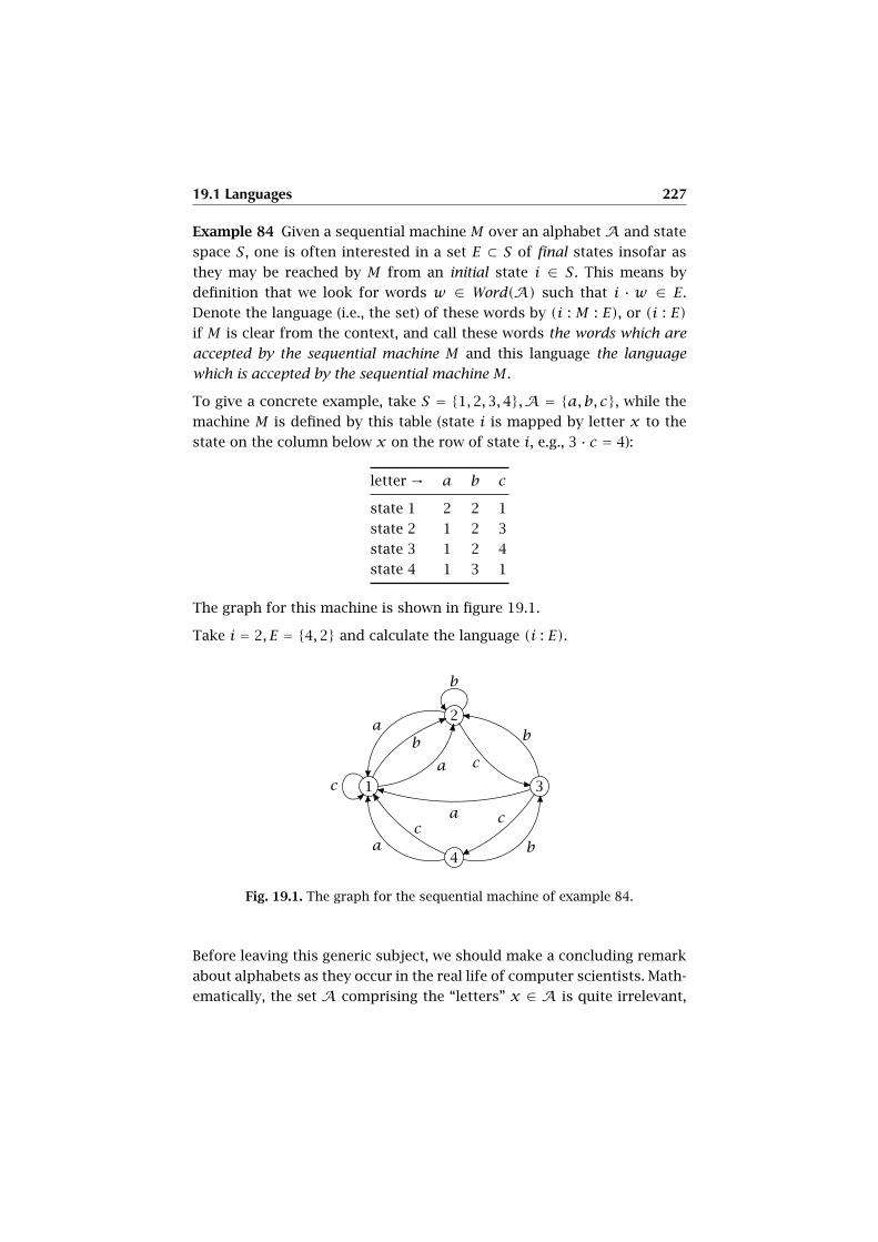
19.1 Languages 227
Example 84 Given a sequential machine M over an alphabetA and state
space S, one is often interested in a set E ⊂ S of final states insofar as
they may be reached by M from an initial state i ∈ S. This means by
definition that we look for words w ∈ Word(A) such that i · w ∈ E.
Denote the language (i.e., the set) of these words by (i : M : E), or (i : E)
if M is clear from the context, and call these words the words which are
accepted by the sequential machine M and this language the language
which is accepted by the sequential machine M .
To give a concrete example, take S = {1,2,3,4},A = {a,b, c}, while the
machine M is defined by this table (state i is mapped by letter x to the
state on the column below x on the row of state i, e.g., 3 · c = 4):
letter → a b c
state 1 2 2 1
state 2 1 2 3
state 3 1 2 4
state 4 1 3 1
The graph for this machine is shown in figure 19.1.
Take i = 2, E = {4,2} and calculate the language (i : E).
1
2
3
4
a
ba
c
b
a c
b
ca
c
b
Fig. 19.1. The graph for the sequential machine of example 84.
Before leaving this generic subject, we should make a concluding remark
about alphabets as they occur in the real life of computer scientists. Math-
ematically, the set A comprising the “letters” x ∈ A is quite irrelevant,
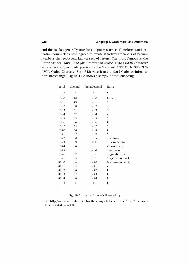
228 Languages, Grammars, and Automata
and this is also generally true for computer science. Therefore standard-
ization committees have agreed to create standard alphabets of natural
numbers that represent known sets of letters. The most famous is the
American Standard Code for Information Interchange (ASCII) character
set codification, as made precise by the Standard ANSI X3.4-1986, “US-
ASCII. Coded Character Set - 7-Bit American Standard Code for Informa-
tion Interchange”. Figure 19.2 shows a sample of that encoding.1
octal decimal hexadecimal Name
......
......
060 48 0x30 0 (zero)
061 49 0x31 1
062 50 0x32 2
063 51 0x33 3
064 52 0x34 4
065 53 0x35 5
066 54 0x36 6
067 55 0x37 7
070 56 0x38 8
071 57 0x39 9
072 58 0x3a : (colon)
073 59 0x3b ; (semicolon)
074 60 0x3c < (less than)
075 61 0x3d = (equals)
076 62 0x3e > (greater than)
077 63 0x3f ? (question mark)
0100 64 0x40 @ (commercial at)
0101 65 0x41 A
0102 66 0x42 B
0103 67 0x43 C
0104 68 0x44 D
......
......
Fig. 19.2. Excerpt from ASCII encoding.
1 See http://www.asciitable.com for the complete table of the 27 = 128 charac-
ters encoded by ASCII.

19.2 Grammars 229
Here, the octal representation refers to the 8-ary representation of num-
bers, whereas the hexadecimal refers to basis 16. One has the following
prefix notations in order to distinguish different adic representations: bi-
nary and decimal numbers have no prefix, octal numbers have the prefix
0, and hexadecimal numbers start with 0x.
Thus ASCII sets up a bijection of the integer interval [0,127] and a set
of relevant characters, predominantly used in the Angloamerican culture.
However, as computers have spread over all cultures, more comprehen-
sive character and sign types have been included in the standardization,
ultimately leading to the Unicode standard. This is a 16-bit character set
standard, designed and maintained by the non-profit consortium Uni-
code Inc. Parallel to the development of Unicode an ISO/IEC standard
was worked on, putting a large emphasis on being compatible with ex-
isting character codes such as ASCII. Merging the ISO (International Or-
ganization for Standardization) standard effort and Unicode in 1992, the
Basic Multilingual Plane BMP was created. But presently the BMP is half
empty, although it covers all major languages, including Roman, Greek,
Cyrillic, Chinese, Hiragana, Katakana, Devanagari, Easter Island “rongo-
rongo”, and even Elvish (but leaves out Klingon).2
19.2 Grammars
We evidently need means to classify languages, since to date the Baby-
lonian variety of languages is beyond control: just imagine all possible
languages based on the traditional European alphabet. We are rightly
confused by the world’s variety of dead or living languages, and by the
ever growing variety of computer languages. A natural way to access lan-
guages is a rule system which directly produces language items, i.e., a
grammatical construction which we also use in natural language to build
new sentences from given ones and from phrase building schemes. Ob-
serve that this is a totally different approach to languages as compared
to the language construction by a sequential machine introduced in the
above example 84. We shall however relate these approaches in the fol-
lowing section 19.3 on automata.
2 See http://www.unicode.org for more information about the Unicode stan-
dard.
230 Languages, Grammars, and Automata
Definition 132 Given an alphabet A, a production grammar over A is a
map
f : Lang(A)→ Lang(A)which commutes with unions, i.e., for any family (Li)i∈I of languages Li
overA, we have
f(⋃
I
Li) =⋃
I
f(Li),
in particular f(∅) = ∅. Ifw ∈ Word(A) is a word, we set f(w) = f({w})and obtain a restricted map f : Word(A) → Lang(A) : x , f(x), which
we denote by the same symbol. One then has
f(L) =⋃
x∈Lf(x)
for any language L ∈ Lang(A). Conversely, if we are given any map
g : Word(A) → Lang(A) : x , f(x), we obtain a production grammar
(again denoted by the same symbol) f : Lang(A) → Lang(A) defined by
the above formula f(L) = ⋃x∈L f(x). In examples, we shall use either
definition according to the concrete situation.
If a production grammar is such that f(x) is always a singleton set, i.e.,
f(x) = {y} for all x ∈ Word(A), then one calls f deterministic, oth-
erwise, it is called nondeterministic. For a deterministic f , we also write
f(x) = y instead of f(x) = {y}.Given a production grammar f : Lang(A) → Lang(A) and an initial lan-
guage I ∈ Lang(A), one has the language f∞(I) generated by f starting
from I, i.e., f∞(I) = ⋃0≤i f i(I) with f 0 = Id and f i = f ◦ f ◦ . . . f , i
times, for positive i. If we are also given a language of terminals T , the
language generated starting from I and terminating in T is defined by
(I : f : T) = T ∩ f∞(I). If the production grammar f is clear, one also
writes (I : T) instead of (I : f : T). For a given alphabetA, two production
grammars f1 and f2 with initial and terminal languages I1 and I2 and T1
and T2, respectively, are called equivalent iff (I1 : f1 : T1) = (I2 : f2 : T2).
Example 85 L-systems are a type of production grammar proposed by
biologist Aristid Lindenmayer in 1968 to provide an axiomatic descrip-
tion of plant growth. We give a simple example of a so-called turtle
graphics production grammar t to illustrate the power of L-systems for
the production of complex graphical objects associated with the lan-
guage t∞(I). One starts with a small alphabet A = {F,G,+,-}, a gram-
mar t = tw1,...wn which is defined by a finite set {w1, . . .wn} of words

19.2 Grammars 231
and the function t = tw1,...wn(x) = {x|w1, . . . x|wn} on words x, where
x|w denotes the word deduced from x by replacing each appearance
of the letter F by w. For example, if x = F-FG+F and w = FG-F, then
x|w = FG-F-FG-FG+FG-F.
Let us consider the deterministic case tw ,w = F-FG+F with one initial
word x0 = FG, i.e., I = {x0 = FG}. Then the language t∞w(x0) is the infinite
set
{FG,F-FG+FG,F-FG+F-F-FG+FG+F-FG+FG . . .}.The turtle language graphically interprets letters and words as follows:
Read a word as a sequence of commands from left to right, so F+FG
means: First do F, then do +, then do F, then do G. The command as-
sociated with F is this: You are a turtle moving on a white paper surface.
Whenever you move, you leave a trace of ink on the surface. Now, doing
F in a word where we have k appearances of the letter x means that the
turtle has a given direction and moves on a straight line of defined length1k . Doing G means that the turtle draws a circle of diameter 1
4k around
its center, but then recovers its position after drawing the circle. Doing
+ means that the turtle just turns clockwise by 90 degrees around its
center, whereas - means a counter-clockwise turn by 90 degrees.
What is the graphical interpretation of the production rule x , x|w?
It means that every straight line segment in the turtle drawing defined
by x is replaced by the drawing defined by w placed in the direction of
that line and shrunk by the factor k such that the total length of the
drawing remains constant, i.e., 1 in our case. This is also why L-systems
are labeled “rewriting systems”. Observe that in contrast to F, the action
G is not rewritten, it is a kind of “terminal” entity.
Fig. 19.3. The graphical interpretation of the first three words of the
L-system featured in example 85.
232 Languages, Grammars, and Automata
An important class of production grammars is described by the following
definition:
Definition 133 We are given a finite alphabet A = T ∪N , which is the
disjoint union of two subsets of letters: the (lower case) terminal symbols
t ∈ T and the (upper case) nonterminal symbols X ∈ N . We are also
given a start symbol S ∈ N and a relation R ⊂ (Word(A)−Word(T ))×Word(A). The production grammar fT ,N ,S,R is defined by the quadruple
(T ,N , S, R) on words x ∈ Word(A) as follows:
fT ,N ,S,R(x) = {x}if there is no u ∈ pr1(R), a, b ∈ Word(A) with x = aub
fT ,N ,S,R(x) = {y | there are words a,b and (u,v) ∈ Rsuch that x = aub and y = avb}
otherwise.
The quadruple (T ,N , S, R), together with the production grammar it de-
fines, is called a phrase structure grammar. In this context, the language
(S : Word(T )) is called the language generated by the phrase structure
grammar (T ,N , S, R). If y ∈ fT ,N ,S,R(x), one also writes x → y and says
that y is obtained from x by application of the rules R. This applies in
particular if (x,y) ∈ R, then one says for x → y that x is the pattern
for the replacement y . If f(x) is a finite set {y1, y2, . . . yr}, then one also
writes x → y1|y2| . . . yr .
Remark 24 We should add a remark here concerning the question when
two languages L and L′ are identical. By definition, there are two alpha-
bets A and A′ such that L ⊂ Word(A) and L′ ⊂ Word(A′). Saying that
the sets L and L′ are the same means that their elements coincide, i.e.,
the words in L and in L′ are the same, and this means that they are the
same sequences of letters from A and A′ respectively. In other words,
there is a common subset A′′ ⊂ A ∩A′ such that L ⊂ Word(A′′) and
L′ ⊂ Word(A′′) and that these subsets are equal. In the above definition
of a language (S : Word(T )) generated by a phrase grammar, this ap-
plies in the sense that neither the set of nonterminals nor the total set
of terminals is relevant to the definition of (S : Word(T )), it is only the
set-theoretic identification which counts.
19.2 Grammars 233
19.2.1 The Chomsky Hierarchy
We now discuss the four-fold hierarchy
type 3 ⊂ type 2 ⊂ type 1 ⊂ type 0
of successively more comprising language types introduced by Noam
Chomsky. In the following discussion of Chomsky types, we suppose that
in a phrase structure grammar (T ,N , S, R), the sets T ,N and R are all
finite. To begin with, we look at the innermost set of languages, those of
type 3.
Definition 134 If for a phrase structure grammar (T ,N , S, R), every rule
x → y in R has the shape X → Yt (X → tY) or X → s for nonterminal
letters X and Y and terminal letters s and t, the grammar is called left
linear (right linear). If a rule X → ε is also admitted in a left linear (right
linear) phrase structure grammar, it is called left (right) regular.
Proposition 158 For a language L the following four properties are equiv-
alent:
(i) There is a left linear phrase structure grammar which generates the
language L− {ε}.(ii) There is a right linear phrase structure grammar which generates
the language L− {ε}.(iii) There is a left regular phrase structure grammar which generates
the language L.
(iv) There is a right regular phrase structure grammar which generates
the language L.
Proof (i) implies (iii): If the left linear phrase structure grammar Gl =(T ,N , S, R) generates L − {ε} (it cannot generate ε, by the nature of its rules).
If ε ∈ L, then we add a new nonterminal element S0 and the rules S → S0 and
S0 → ε, and the new left regular phrase structure grammar does the job.
(iii) implies (i): If the left regular phrase structure grammar (T ,N , S, R) gener-
ates L, and ε ∈ L, then we successively reduce the number of nonterminals X
which have the rule X → ε until they have disappeared. The crucial the case is
X → ε, when this is the only rule for X on the left side. If we omit this rule, we
not only prevent ε from being generated, but all the words stemming from a rule
Y → xX followed by X → ε are in danger. Therefore, we have to add the rule
Y → x for each Y → xX, then we can omit X → ε, and are done.

234 Languages, Grammars, and Automata
The proof for the right linear cases ((ii) iff (iv)) works the same way, therefore we
omit it.
We are left with the equivalence of left linear and right linear generation of lan-
guages, i.e., (i) iff (ii). We show that (i) implies (ii), the converse follows by ex-
changing left and right. To begin with, we may choose a new start symbol S ′
and add to every rule S → ? a rule S ′ → ?. Then the new grammar never has its
start symbol on the right hand side of any rule and is of course equivalent to
the original. So we may suppose wlog that S never appears on the right side of
a rule. We then construct a right linear grammar Gr = G∗l which is equivalent to
Gl. But we construct more: The rules of Gr are such that the same operator ∗,
when applied to Gr , with left and right exchanged, yields ∗Gr = Gl.This is the new rule set R∗, the alphabet being unaltered:
1. The rules S → t are left unchanged.
2. A rule S → Xs is replaced by the rule X → s.3. A rule X → s with X ≠ S, is replaced by the rule S → sX.
4. A rule X → Yt with X ≠ S, is replaced by the rule Y → tX.
We now show that (S : R : T ) ⊂ (S : R∗ : T ). The converse is true by exchanging
the roles of left and right and by the remark that the star operator, when applied
to Gr gives us back Gl. The proof is by induction on the length n of a path S →Xs → . . .w with w ∈ (S : R : T ). For n = 1 this is rule 1. If S → Xs → . . . vu = win Gl has length n+ 1, where the path Xs → . . . vu has length n and stems from
the length n path X → . . . v , then we show that we have a path S → . . . vX → vuin Gr . We show by induction on path length, that if X → . . . v in Gl has length
m, then there is a path S → vX of length m in Gr . For m = 1, this is rule 3. In
general, we have X → Yx → . . . yx = v , where the rule X → Yx in R is converted
into the rule Y → xX in R∗ according to rule 4 above. By induction hypothesis
we now have this new path: S → . . . yY → yxX = vX, the first part being implied
from Y → . . . y to the right of X → Yx → . . . yx, and we are done. �
Definition 135 A language which shares the equivalent properties of
proposition 158 is called regular or of type 3.
The crucial fact about type 3 languages is this:
Proposition 159 If L, L′ ∈ Lang(A) are of type 3 (i.e., regular), then so
are
L∪ L′, L∩ L′, L∗, LL′,Word(A)− L.Languages of type 3 are closed under all boolean operations as well as the
Kleene operator and the product of languages.
19.2 Grammars 235
Proof The proof idea is exemplified for the statement of L ∪ L′ being of type
3 if L and L′ are so. Take two phrase structure grammars G = (T ,N , S, R) and
G′ = (T ,N ′, S′, R′) which generate L and L′, respectively. It is clear that one
may suppose that the nonterminal sets N and N ′ are disjoint. From the proof
of proposition 158, we may also assume that the start symbols S and S ′ are never
on the right side of a rule. But then we create a new setN ∗ =N∪N ′∪{S∗} with
a new start symbol S∗ not inN andN ′, while the old rules are inherited, except
for the rules S → w,S′ → w′, which we replace by the rules S∗ → w,S∗ → w′,and we are done. We refer to [43] for a complete proof. �
Example 86 Let T = {a,b, c} and N = {S,A, B, C} and consider the
language L1 = {albmcn | l > 0,m > 0, n > 0}. A right linear grammar for
this language consists of the rules R1 = {S → aA,A → aA,A → bB, B →bB, B → cC, B → c, C → cC,C → c}. A right regular grammar can be
expressed with the (simpler) set of rules RR1 = {S → aA,A → aA,A →bB, B → bB, B → cC,C → cC,C → ε}. Note the different handling of the
end of words. A regular grammar can also be found for the language
L2 = {albmcn | l ≥ 0,m ≥ 0, n ≥ 0}, with the rules R2 = {S → A,A →aA,A → B, B → bB, B → C,C → cC,C → ε}. For L2 no linear grammar
exists.
A left linear grammar for L1 is given by the rules RL1 = {S → Bc, S →Cc,C → Cc,C → Bc, B → Bb, B → Ab,A → Aa,A → a}. Using this gram-
mar a derivation for the word abcc is given as follows:
S → Cc→ Bcc→ Abcc→ abcc
A useful property of languages of type 3 is embodied by the following
lemma:
Lemma 160 (Type 3 Pumping Lemma) Let G = (T ,N , S, R) be a linear
grammar and L the language generated by G. Let x ∈ L where l(x) >
card(N ). Then there exist words x, z,w ∈ Lang(T ), z ≠ ε, such that
x = yzw and yzkw ∈ L for k = 0,1, . . . .
Proof Consider a word x of length |x| > |N |. Then a derivation consists of
|x| steps. Since the number of nonterminals is less than |x|, there must be a
subderivation of length at most |N | that begins with a nonterminal, say A, and
236 Languages, Grammars, and Automata
ends with the same non-terminal A, e.g. S → . . . yA → . . . yzA → . . . yzw. But
the subderivation A → . . . zA, can be substituted for the second A, thus yielding
yzzw, and again, yzzzw, and so on. The subderivation can be left out entirely,
yielding yw. �
The languages of type 2 are the context free languages which may be used
to describe programming languages, mainly in its wide-spread Backus-
Naur form (BNF), and more standardized as augmented BNF (ABNF) or
the extended BNF (EBNF) (standard ISO 14977); see 19.2.2 below for this
type of grammars.
Definition 136 A phrase structure grammar (T ,N , S, R), with alphabet
A= T ∪N is said to be
(i) context free if its rules are all of shape X → x with X ∈ N and
x ∈ Word(A);(ii) reduced if it is context free and for each nonterminal A different
from the start symbol S, there is a rule A → t with t ∈ T terminal,
and for each nonterminal A ∈ N , there is a rule S → vAw with
v,w ∈ Word(A);(iii) in Chomsky normal form if its rules are of shape X → t or X → AB
for X,A, B ∈N and t ∈ T ;
(iv) in Greibach normal form if its rules are of shape X → xw with
X ∈N , x ∈ T , and w ∈ Word(N ).
Proposition 161 For a language L the following four properties are equiv-
alent:
(i) There is a context free phrase structure grammar which generates
the language L.
(ii) There is a reduced context free phrase structure grammar which
generates the language L.
(iii) There is a phrase structure grammar in Chomsky normal form
which generates the language L− {ε}.(iv) There is a phrase structure grammar in Greibach normal form
which generates the language L− {ε}.Proof We have given a proof of proposition 158. The proof of this proposition
is however too long for our context, therefore we refer to [43]. �
Definition 137 A language which shares the equivalent properties of
proposition 161 is called context free or of type 2.
19.2 Grammars 237
By virtue of the first criterion in definition 136, a language of type 3 is
evidently of type 2. The crucial fact about type 2 languages is this:
Proposition 162 If L, L′ ∈ Lang(A) are of type 2 (i.e., context free), then
so are
L∪ L′, L∗ and LL′.
Proof Again, we give an idea of the proof for the union L ∪ L′. Take the defini-
tion 136, (i), for two type 2 languages L and L′. Let two phrase structure gram-
mars G = (T ,N , S, R) and G′ = (T ,N ′, S′, R′) generate languages L and L′,respectively. One may again assume that the sets N and N ′ of nonterminals
are disjoint. Then just take the union ofN andN ′ and add a new start symbol
S∗, together with the two rules S∗ → S and S∗ → S′, which solves the problem.
We refer to [43] for a complete proof. �
There exists also a pumping lemma for languages of type 2:
Lemma 163 (Type 2 Pumping Lemma) Let L be context free. Then there
exists n such that for every x ∈ L with l(x) ≥ n there exist words
u,v,y, z,w where v ≠ ε or z ≠ ε such that x = uvyzw and uvkyzkw ∈L for k = 0,1, . . .
Proof See [28] for a proof. �
Example 87 We can use a context free grammar to describe expres-
sions of elementary arithmetic. Expressions of this type are common
in the syntax of programming languages. Let N = {S, E, F, T} and take
T = {+,∗, (, ),x,y,z} where the letters x, y and z denote variables in
the programming language. The rules are given by R = {E → T+E, E →T , T → F∗T , T → F, F → (E), F → x|y|z}.A derivation of the expression x+ y∗ (z+ y) is given in figure 19.4.
Note how the rules model the usual precedence rules of the operators +and ∗. This is of great practical value when implementing a parser for an
actual programming language.
Figure 19.5 shows the derivation in form of a syntax tree. Each node of
the tree is an application of a rule, the resulting expression can be read
off the leaves of the tree in left-to-right order.
Exercise 88 Not every language of type 2 is of type 3, i.e., the inclusion
type 3 ⊂ type 2 is proper. Construct a context free grammar for the lan-
guage L = {anbn | n ≥ 1} overA = {a,b}, then use the pumping lemma
for type 3 languages to show that there is no regular grammar for L.

238 Languages, Grammars, and Automata
E → T + E→ F + E→ x+ E→ x+ T→ x+ F ∗ T→ x+ y∗ T→ x+ y∗ F→ x+ y∗ (E)→ x+ y∗ (T + E)→ x+ y∗ (F + E)→ x+ y∗ (z+ E)→ x+ y∗ (z+ T)→ x+ y∗ (z+ F)→ x+ y∗ (z+ y)
Fig. 19.4. A derivation of the expression x+ y∗ (z+ y)
Definition 138 A phrase structure grammar (T ,N , S, R), with alphabet
A = T ∪N is said to be context sensitive iff for every rule x → y in R,
we have l(x) ≤ l(y). A language is called context sensitive or of type 1
iff it is generated by a context sensitive phrase structure grammar.
Evidently, the characterization of context free languages by Chomsky nor-
mal form grammars implies that type 2 is a subset of type 1. The crucial
fact about type 1 languages is this:
Proposition 164 If L ∈ Lang(A) are of type 1 (i.e., context sensitive), then
so is its complement language Word(A)− L.
Proof We refer to [43] for a proof. �
Example 88 Let T = {a,b, c} and N = {S,A, B, C,D, E}. The language
L = {akbkck | k > 0} is of type 1. The rather complicated grammar is
given by the following set of rules: R = {S → Abc,A → a,A → aB, B →aC,Cb → bC,Cc → Dc,D → bc,D → Ebc, bE → Eb,aE → aB}. Let us see
how this works on the example of the word aaabbbccc:

19.2 Grammars 239
S → Abc→ aBbc→ aaCbc→ aabCc→ aabDc→ aabEbcc→ aaEbbcc→ aaBbbcc→ aaaCbbcc→ aaabCbcc→ aaabbCcc→ aaabbDcc→ aaabbbccc
Fig. 19.5. The syntax tree for x+ y∗ (z+ y).

240 Languages, Grammars, and Automata
We have yet to prove that there is no grammar of type 2 generating this
language. We do this by invoking the type 2 pumping lemma 163. Sup-
pose that L is context free. The lemma assures, that there is a number n
such that the properties of the lemma will be fulfilled for words of length
≥ n. Let us choose the word anbncn ∈ L which is certainly longer than
n. The lemma tells us that this word must have a structure uvyzw such
that uvkyzkw ∈ L for k = 0,1, . . .. But however we choose two subwords
in anbncn, the resulting “pumped-up” word will not be in L. Either the
equal number of as, bs and cs will not be maintained, or the order of the
letters will not be respected, as can be easily checked. Thus L cannot be
context free.
Exercise 89 Prove, by finding a counterexample, that the intersection of
two context free languages need not be context free.
The last type 0 is that of completely general phrase structure grammars:
Definition 139 A phrase structure grammar (T ,N , S, R), with alphabet
A= T ∪N is called
(i) general if there are no further conditions,
(ii) separated if each of its rules x → y has one of the following shapes:
a) x ∈ Word(N )− {ε} with y ∈ Word(N ),b) x ∈N with y ∈ T , or
c) x ∈N with y = ε,(iii) normal if each of its rules x → y has one of the following shapes:
a) x ∈N with y ∈ T ,
b) x ∈N with y = ε,c) x ∈N with y ∈N 2, or
d) x,y ∈N 2.
It should be stressed that the definition (i) “general phrase structure
grammar” is redundant, but has been used in the computer community
as a synonym of “phrase structure grammar”. So the following proposi-
tion effectively is a statement about phrase structure grammars without
any further attribute.
Proposition 165 For a language L the following four properties are equiv-
alent:
19.2 Grammars 241
(i) There is a (general) phrase structure grammar generating L.
(ii) There is a separated phrase structure grammar generating L.
(iii) There is a normal phrase structure grammar generating L.
Proof We refer to [43] for a proof. �
Definition 140 A language L which shares the equivalent properties of
proposition 165 is called recursively enumerable or of type 0.
19.2.2 Backus-Naur Normal Forms
The syntax of most programming languages, e.g., Algol, Pascal, C or Java,
can be described by context free grammars. Originally, BNF was used by
Peter Naur for the description of Algol 60 in an adaptation of a notation
developed by John Backus.
The idea was to set up a standardized formal procedure to create termi-
nal and nonterminal symbols and to describe the rules. Recall that the
rules in context free grammars have the particular form X → w, where
w ∈ Word(A) and X is a nonterminal symbol. To begin with, the ar-
row “→” in a rule is replaced by the sign “::=” derived from the math-
ematical symbol “:=” meaning that x is defined by y in the expression
x := y . The alternative x → y1|y2| . . . yn is written analogously, i.e., by
x ::= y1|y2| . . . yn.
The more important contribution of BNF is that the terminal and non-
terminal symbols are provided by a standard construction from a given
character set CH , in the ASCII encoding, say, i.e., “CH = ASCII”. The pro-
cedure is very simple: Terminals are just single characters from CH . Non-
terminals are all words of shape 〈w〉,w ∈ Word(CH). The start symbol is
mostly clear from the given rule system. For example, the Algol 60 spec-
ification of a floating point constant is called “<unsigned number>”, and
this is the start symbol, which defines the sublanguage of floating-point
constants as follows:
<unsigned integer> ::= <digit> | <unsigned integer> <digit>
<integer> ::= <unsigned integer> | + <unsigned integer> |
- <unsigned integer>
<decimal fraction> ::= . <unsigned integer>
<exponent part> ::= _10_ <integer>
<decimal number> ::= <unsigned integer> | <decimal fraction> |
242 Languages, Grammars, and Automata
<unsigned integer> <decimal fraction>
<unsigned number> ::= <decimal number> | <exponent part> |
<decimal number> <exponent part>
<digit> ::= 0|1|2|3|4|5|6|7|8|9
Here, the start symbol is S = <unsigned number>. In comparison, the
Extended BNF notation (EBNF) of the same grammar is this:
unsigned integer = digit | unsigned integer, digit;
integer = unsigned integer | "+", unsigned integer |
"-", unsigned integer;
decimal fraction = ".", unsigned integer;
exponent part = "_10_", integer;
decimal number = unsigned integer | decimal fraction |
unsigned integer, decimal fraction;
unsigned number = decimal number | exponent part |
decimal number, exponent part;
digit = "0"|"1"|"2"|"3"|"4"|"5"|"6"|"7"|"8"|"9";
The EBNF notation also includes some extensions to BNF, which improvereadability and conciseness, e.g., the Kleene cross for a sequence of oneor more elements of the class so marked, for example
unsigned integer = digit+;
The changes are evident, the idea behind this standardization is clear and
is usually learned by doing some examples.3
It is also customary to represent a BNF grammar by use of syntax di-
agrams, i.e., groups of flow charts, where the alternatives in a rule
X ::= y1|y2| . . . yn are flow ramifications starting from the block of X and
terminating at the leftmost symbol in the target replacement yi. Here, the
leaves are the terminal symbols. Figure 19.6 is a syntax diagram; such di-
agrams were used for the first time by Jensen and Wirth.
Exercise 90 Define (the fragments of) an alphabet and write the BNF
rules corresponding to the flow charts shown in figure 19.6.
3 See http://www.cl.cam.ac.uk/˜mgk25/iso-14977-paper.pdf for a more
complete description of the BNF standard.
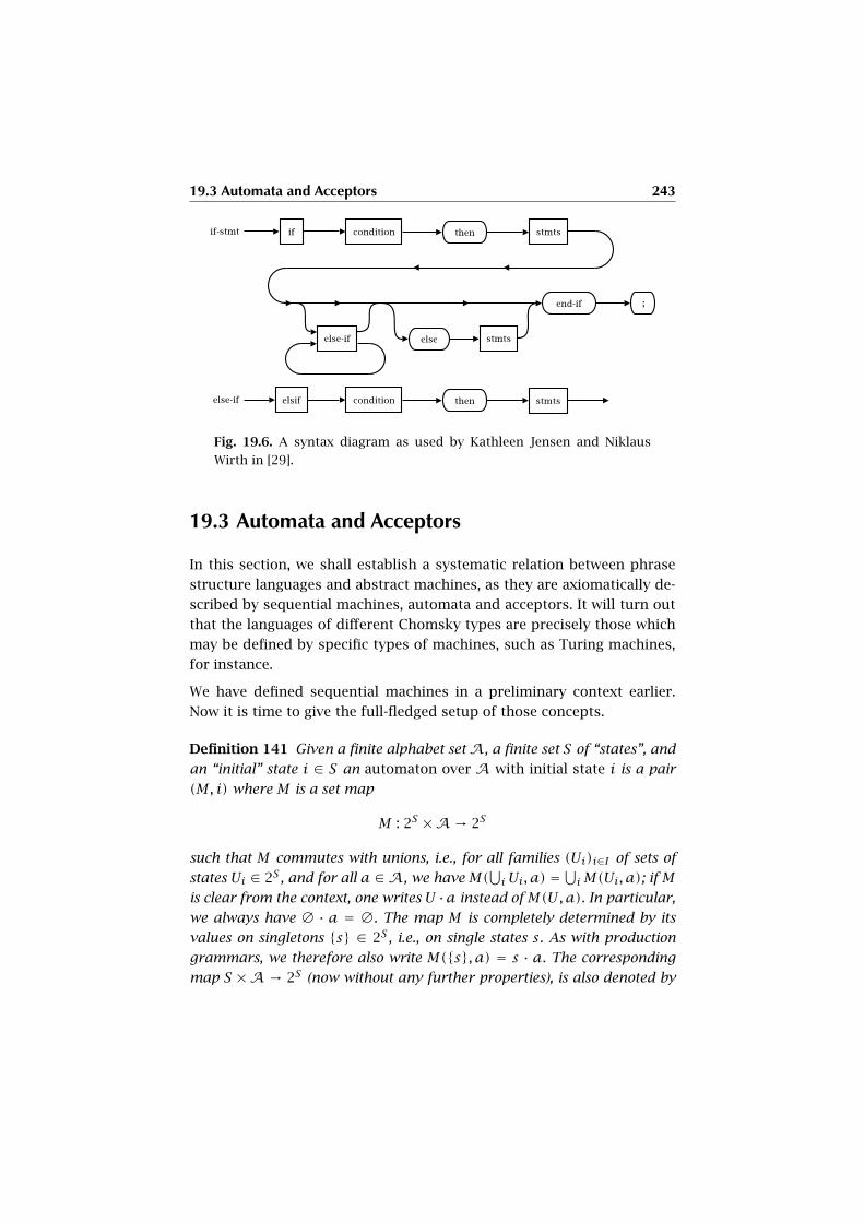
19.3 Automata and Acceptors 243
Fig. 19.6. A syntax diagram as used by Kathleen Jensen and Niklaus
Wirth in [29].
19.3 Automata and Acceptors
In this section, we shall establish a systematic relation between phrase
structure languages and abstract machines, as they are axiomatically de-
scribed by sequential machines, automata and acceptors. It will turn out
that the languages of different Chomsky types are precisely those which
may be defined by specific types of machines, such as Turing machines,
for instance.
We have defined sequential machines in a preliminary context earlier.
Now it is time to give the full-fledged setup of those concepts.
Definition 141 Given a finite alphabet setA, a finite set S of “states”, and
an “initial” state i ∈ S an automaton over A with initial state i is a pair
(M, i) where M is a set map
M : 2S ×A→ 2S
such that M commutes with unions, i.e., for all families (Ui)i∈I of sets of
states Ui ∈ 2S , and for all a ∈A, we have M(⋃iUi, a) =
⋃iM(Ui, a); if M
is clear from the context, one writes U ·a instead ofM(U,a). In particular,
we always have ∅ · a = ∅. The map M is completely determined by its
values on singletons {s} ∈ 2S , i.e., on single states s. As with production
grammars, we therefore also write M({s}, a) = s · a. The corresponding
map S ×A → 2S (now without any further properties), is also denoted by
244 Languages, Grammars, and Automata
M and serves as an alternate definition for an automaton, much as this
was done for production grammars.
An automaton is called deterministic if its images s · a on singletons are
always singletons s · a = {x} (attention: in particular, the images s · aare never empty!). We then also write s · a = x, and correspondingly M :
S×A→ S. A nondeterministic automaton is one which is not deterministic.
The elementary graph of an automaton is the digraph ΓM : Arr(M) → S2
the arrow set of which is Arr(M) = {(s, a,x) | a ∈ A, s ∈ S,x ∈ s · a}with ΓM((s, a,x)) = (s, x). The initial state i is rephrased as a morphism
of digraphs i : 1→ ΓM pointing to the vertex i. A path
p = s1 (s1,a1,s2)ñ s2
(s2,a2,s3)ñ s3 . . .
(sm−1,am−1,sm)ñ sm
in ΓM starting at the initial state i (i.e., with s1 = i) is called a state sequence
of the automaton associated with the word Wp = a1a2 . . . am. The lazy
path is associated with the empty word.
Evidently, every automaton (M, i) determines its alphabet A and state
set S, so we do not need to mention them explicitly.
Any automaton defines the associated power automaton (M ′, i′), which,
evidently, is always deterministic, with these data: We replace S by S ′ =2S and i by i′ = {i}. Then the same map M ′ = M defines an automaton,
but we take the alternate definition M ′ : S′×A→ S′. this time! Using this
definition we don’t need to deal with 22S , as would have been required by
the first definition. This is nothing more than a trick of switching from
the first definition to the second one. The point is that, however, not every
deterministic automaton is of this type, since its state set need not be a
powerset, and the commutation with unions need not work.
Although the elementary graph of an automaton is customary in com-
puter science, it has some serious structural drawbacks which enforce
a second digraph associated with an automaton: the power graph ΓM of
an automaton (i,M) is the elementary graph of the associated power
automaton, ΓM = ΓM′ . Since the power automaton is a priori determin-
istic, the power graph may be described more economically (it is in
fact the Moore graph of the underlying sequential machine, check this
out) as follows: vertexes are the sets of states, its arrows are the pairs
(s, a) ∈ 2S ×A, which are mapped to the state set pairs (s, s ·a), and the
initial state pointer is i′ : 1→ ΓM .
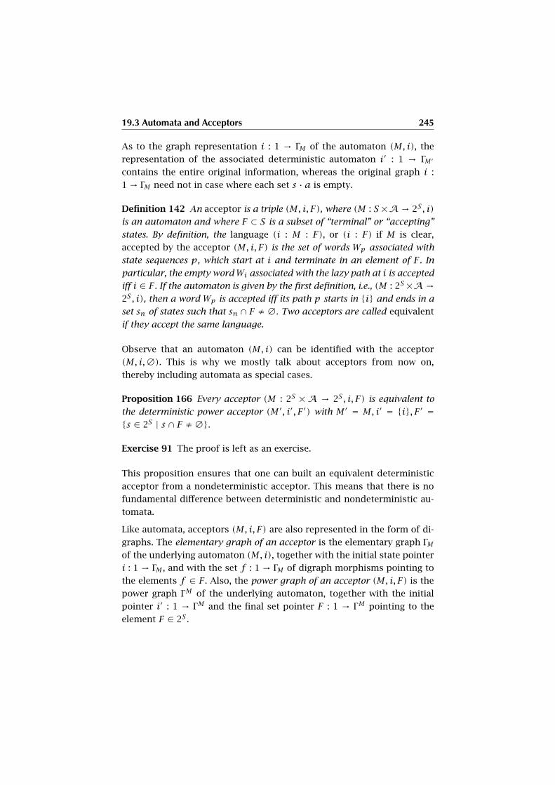
19.3 Automata and Acceptors 245
As to the graph representation i : 1 → ΓM of the automaton (M, i), the
representation of the associated deterministic automaton i′ : 1 → ΓM′
contains the entire original information, whereas the original graph i :
1→ ΓM need not in case where each set s · a is empty.
Definition 142 An acceptor is a triple (M, i, F), where (M : S ×A→ 2S , i)
is an automaton and where F ⊂ S is a subset of “terminal” or “accepting”
states. By definition, the language (i : M : F), or (i : F) if M is clear,
accepted by the acceptor (M, i, F) is the set of words Wp associated with
state sequences p, which start at i and terminate in an element of F . In
particular, the empty wordWi associated with the lazy path at i is accepted
iff i ∈ F . If the automaton is given by the first definition, i.e., (M : 2S×A→2S , i), then a word Wp is accepted iff its path p starts in {i} and ends in a
set sn of states such that sn ∩ F ≠ ∅. Two acceptors are called equivalent
if they accept the same language.
Observe that an automaton (M, i) can be identified with the acceptor
(M, i,∅). This is why we mostly talk about acceptors from now on,
thereby including automata as special cases.
Proposition 166 Every acceptor (M : 2S ×A → 2S , i, F) is equivalent to
the deterministic power acceptor (M ′, i′, F ′) with M′ = M, i′ = {i}, F ′ ={s ∈ 2S | s ∩ F ≠∅}.
Exercise 91 The proof is left as an exercise.
This proposition ensures that one can built an equivalent deterministic
acceptor from a nondeterministic acceptor. This means that there is no
fundamental difference between deterministic and nondeterministic au-
tomata.
Like automata, acceptors (M, i, F) are also represented in the form of di-
graphs. The elementary graph of an acceptor is the elementary graph ΓMof the underlying automaton (M, i), together with the initial state pointer
i : 1 → ΓM , and with the set f : 1 → ΓM of digraph morphisms pointing to
the elements f ∈ F . Also, the power graph of an acceptor (M, i, F) is the
power graph ΓM of the underlying automaton, together with the initial
pointer i′ : 1 → ΓM and the final set pointer F : 1 → ΓM pointing to the
element F ∈ 2S .
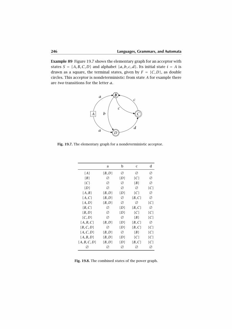
246 Languages, Grammars, and Automata
Example 89 Figure 19.7 shows the elementary graph for an acceptor with
states S = {A,B,C,D} and alphabet {a,b, c, d}. Its initial state i = A is
drawn as a square, the terminal states, given by F = {C,D}, as double
circles. This acceptor is nondeterministic: from state A for example there
are two transitions for the letter a.
A
BB
C
D
a
c
b
c
da
Fig. 19.7. The elementary graph for a nondeterministic acceptor.
a b c d
{A} {B,D} ∅ ∅ ∅{B} ∅ {D} {C} ∅{C} ∅ ∅ {B} ∅{D} ∅ ∅ ∅ {C}{A,B} {B,D} {D} {C} ∅{A,C} {B,D} ∅ {B,C} ∅{A,D} {B,D} ∅ ∅ {C}{B,C} ∅ {D} {B,C} ∅{B,D} ∅ {D} {C} {C}{C,D} ∅ ∅ {B} {C}{A,B,C} {B,D} {D} {B,C} ∅{B,C,D} ∅ {D} {B,C} {C}{A,C,D} {B,D} ∅ {B} {C}{A,B,D} {B,D} {D} {C} {C}{A,B,C,D} {B,D} {D} {B,C} {C}
∅ ∅ ∅ ∅ ∅
Fig. 19.8. The combined states of the power graph.
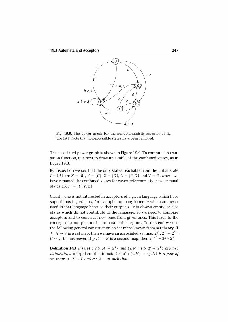
19.3 Automata and Acceptors 247
I
U
Z
V
X
Y
a
b, c, d
a
c,d
b
a,b, c
b
d
c
ca,d
a,b,d
a,b, c, d
Fig. 19.9. The power graph for the nondeterministic acceptor of fig-
ure 19.7. Note that non-accessible states have been removed.
The associated power graph is shown in Figure 19.9. To compute its tran-
sition function, it is best to draw up a table of the combined states, as in
figure 19.8.
By inspection we see that the only states reachable from the initial state
I = {A} are X = {B}, Y = {C}, Z = {D}, U = {B,D} and V = ∅, where we
have renamed the combined states for easier reference. The new terminal
states are F ′ = {U,Y ,Z}.
Clearly, one is not interested in acceptors of a given language which have
superfluous ingredients, for example too many letters a which are never
used in that language because their output s · a is always empty, or else
states which do not contribute to the language. So we need to compare
acceptors and to construct new ones from given ones. This leads to the
concept of a morphism of automata and acceptors. To this end we use
the following general construction on set maps known from set theory: If
f : X → Y is a set map, then we have an associated set map 2f : 2X → 2Y :
U , f(U), moreover, if g : Y → Z is a second map, then 2g◦f = 2g ◦ 2f .
Definition 143 If (i,M : S ×A → 2S) and (j,N : T × B → 2T ) are two
automata, a morphism of automata (σ ,α) : (i,M) → (j,N) is a pair of
set maps σ : S → T and α :A→ B such that
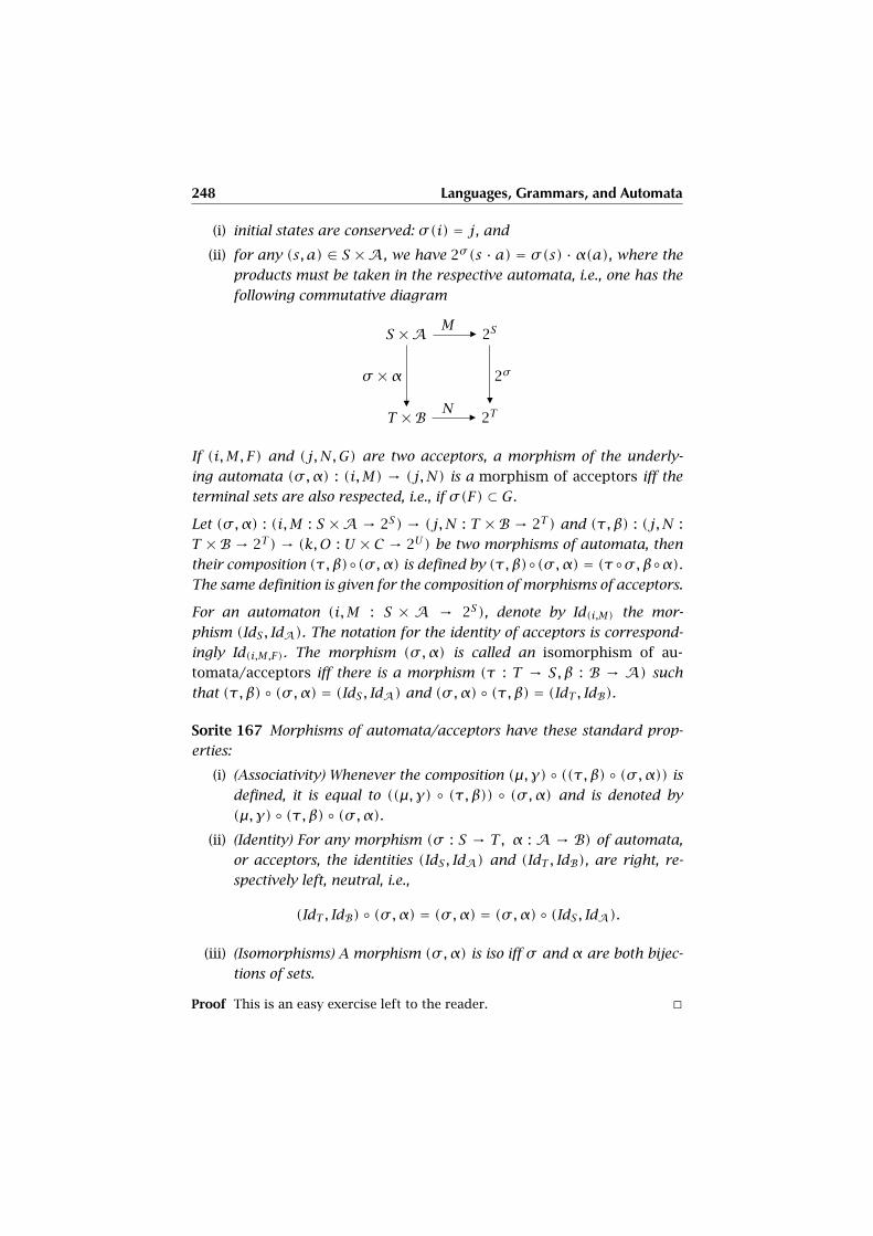
248 Languages, Grammars, and Automata
(i) initial states are conserved: σ(i) = j, and
(ii) for any (s, a) ∈ S ×A, we have 2σ (s · a) = σ(s) · α(a), where the
products must be taken in the respective automata, i.e., one has the
following commutative diagram
S ×A Mñ 2S
T ×B
σ ×α� N
ñ 2T
2σ
�
If (i,M, F) and (j,N,G) are two acceptors, a morphism of the underly-
ing automata (σ ,α) : (i,M) → (j,N) is a morphism of acceptors iff the
terminal sets are also respected, i.e., if σ(F) ⊂ G.
Let (σ ,α) : (i,M : S ×A → 2S) → (j,N : T × B → 2T ) and (τ, β) : (j,N :
T ×B → 2T ) → (k,O : U × C → 2U) be two morphisms of automata, then
their composition (τ, β)◦(σ ,α) is defined by (τ, β)◦(σ ,α) = (τ◦σ,β◦α).The same definition is given for the composition of morphisms of acceptors.
For an automaton (i,M : S × A → 2S), denote by Id(i,M) the mor-
phism (IdS , IdA). The notation for the identity of acceptors is correspond-
ingly Id(i,M,F). The morphism (σ ,α) is called an isomorphism of au-
tomata/acceptors iff there is a morphism (τ : T → S, β : B → A) such
that (τ, β) ◦ (σ ,α) = (IdS , IdA) and (σ ,α) ◦ (τ, β) = (IdT , IdB).
Sorite 167 Morphisms of automata/acceptors have these standard prop-
erties:
(i) (Associativity) Whenever the composition (µ, γ) ◦ ((τ, β) ◦ (σ ,α)) is
defined, it is equal to ((µ, γ) ◦ (τ, β)) ◦ (σ ,α) and is denoted by
(µ, γ) ◦ (τ, β) ◦ (σ ,α).(ii) (Identity) For any morphism (σ : S → T , α : A → B) of automata,
or acceptors, the identities (IdS , IdA) and (IdT , IdB), are right, re-
spectively left, neutral, i.e.,
(IdT , IdB) ◦ (σ ,α) = (σ ,α) = (σ ,α) ◦ (IdS , IdA).
(iii) (Isomorphisms) A morphism (σ ,α) is iso iff σ and α are both bijec-
tions of sets.
Proof This is an easy exercise left to the reader. �
19.3 Automata and Acceptors 249
Exercise 92 Let (σ ,α) : (i,M : S ×A → 2S) → (j,N : T × B → 2T ) be a
morphism of automata, show that the map (s, a,x), (σ(s),α(a),σ(x))
on arrows and σ on vertexes defines a morphism Γ(σ ,α) : ΓM → ΓN which
also maps the initial pointers into each other. Also, if we have sets of final
states and therefore acceptors, the corresponding pointers to final states
are preserved. Show that on power graphs ΓM and ΓN we have a corre-
sponding morphism Γ (σ ,α) : ΓM → ΓN defined by 2σ × α on arrows and
2σ on vertexes. Show that for two morphisms (τ, β) and (σ ,α) which
can be composed to (τ, β) ◦ (σ ,α), we have Γ(τ,β)◦(σ ,α) = Γ(τ,β) ◦ Γ(σ ,α)and Γ (τ,β)◦(σ ,α) = Γ (τ,β) ◦ Γ (σ ,α). This kind of passage from one type of
objects (automata) to another type (digraphs), which also preserves mor-
phisms and their composition, is called functorial and will be discussed
extensively in the second volume of this book dedicated to so-called cate-
gories. Categories are a fundamental subject in modern mathematics and
are becoming more and more important in computer science.
Proposition 168 If (σ : S → T ,α : A → B) is a morphism of acceptors
(σ ,α) : (i,M, F) → (j,N,G), then the induced homomorphism of the lan-
guage set Word(α) : Word(A)→ Word(B)maps (i : M : F) into (j : N : G).
If in particular (σ ,α) is an isomorphism, then Word(α) induces a bijec-
tion (i : M : F)∼→ (j : N : G). More specifically, if also α = IdA, then
(i : M : F) = (j : N : G).
Exercise 93 Use the elementary graph of an acceptor and the morphism
Γ(σ ,α) to give a proof of proposition 168.
Definition 144 If (σ ,α) : (i,M, F) → (j,N,G) is a morphism of acceptors
over the alphabets A and B respectively, such that α : A ↩ B and σ :
S ↩ T are subset inclusions, then we say that (i,M, F) is a subacceptor of
(j,N,G).
Corollary 169 If (i,M, F) is a subacceptor of (j,N,G), then (i : M : F) is
a sublanguage of (j : N : G).
Proof This follows immediately from proposition 168. �
Definition 145 An acceptor (i,M, F) is simple iff every state s ∈ S is a
vertex of a state sequence p from i to F .
Proposition 170 Every acceptor has an equivalent simple subacceptor.
250 Languages, Grammars, and Automata
Proof Since the states not appearing in any state sequence have no meaning
for the generated words, one obtains the same language when omitting those
states. �
Besides the simplification procedure for an acceptor, we may also need to
look for subacceptors which are present in multiple “copies”, i.e., which
play the same role with respect to the language they accept. We now
want to eliminate such multiplicities, since it is not reasonable to have
machines with equivalent functional units in multiple instantiations.
Definition 146 IfM is a sequential machine and F ⊂ S a set of final states,
then two states s, t ∈ S are called equivalent if (s : M : F) = (t : M : F). If
for an acceptor (i,M, F) any two different states s ≠ t on state sequences
from i to F are not equivalent, the acceptor is called reduced.
We now discuss the construction of a reduced acceptor from a given de-
terministic acceptor (i,M : S×A→ S, F). To begin with, we need a generic
sequential machine associated with the alphabetA.
Definition 147 For the alphabetA the sequential machine LangMachineAofA is defined by the map
LangMachineA : Lang(A)×A→ Lang(A)(L,a), L/a = {x ∈ Word(A) | a · x ∈ L}.
If (i,M, F) is an acceptor, the associated generic acceptor is defined by
(iA,LangMachineA, FA), where
(i) iA = (i : M : F)
(ii) and FA = {(f : M : F) | f ∈ F}.
Exercise 94 If one defines more generally L/w = {x ∈ Word(A) | w·x ∈L} for w ∈ Word(A), then v,w ∈ Word(A) implies (L/v)/w = L/(vw).
Proposition 171 For a deterministic acceptor (i,M : S ×A → S, F), con-
sider the morphism
(σ , IdA) : (i,M, F)→ (iA,LangMachineA, FA)
of acceptors given by σ(s) = (s : M : F). Then the image (i,M, F)A of
(σ , IdA) is an equivalent reduced deterministic acceptor, more precisely,
for each state s ∈ S we have
(s : M : F) = ((s : M : F) : LangMachineA : FA).
19.3 Automata and Acceptors 251
(i) If (i,M, F) is simple, then so is (i,M, F)A.
(ii) If (i,M, F) is reduced, then (σ , IdA) : (i,M, F) → (i,M, F)A is an
isomorphism.
(iii) If (i,M, F) and (j,N,G) are reduced, simple, and equivalent, then
(i,M, F)A = (j,N,G)A.
Proof To begin with, we have to check whether (σ , IdA) is a morphism. This
readily follows from the fact that for a pair (s, a) ∈ S×A, we have (s ·a,M, F) =(s,M, F)/a. To show that
(s :M : F) = ((s : M : F) : LangMachineA : FA),
letw ∈ (s :M : F). Then s·w ∈ F . Therefore, (s : M : F)·w = (s·w : M : F) ∈ FA,
whence w ∈ ((s : M : F) : LangMachineA : FA), i.e., (s : M : F) ⊂ ((s : M : F) :
LangMachineA : FA). Conversely, if w ∈ ((s : M : F) : LangMachineA : FA),then we have (s : M : F)/w = (f : M : F), f ∈ F . In other words, s ·w · v ∈ Fiff f · v ∈ F , for any word v . In particular, v = ε, the empty word gives us
f · ε = f ∈ F whence s · w · ε = s · w ∈ F , so w ∈ (s : M : F), whence
(s : M : F) ⊃ ((s : M : F) : LangMachineA : FA), and equality holds.
The new acceptor is deterministic by construction, and it is reduced since the
language we obtain in the image ((s : M : F) : LangMachineA : FA) is exactly
the starting state (s : M : F), so no two different starting states can produce the
same language. If (s : M : F) is simple, every state t is visited by a state sequence
starting at s in a wordw. But then the state (s·w,M, F) is reached byw from the
starting point (s,M, F), whence claim (i). As to claim (ii), observe that the fiber of
a state (s,M, F) is the set of states t which generate the same language (t,M, F),
i.e., the equivalent states of the (possibly) not reduced acceptor. Therefore, if
all fibers are singletons, the map on states is a bijection, and we are done. To
prove (iii), observe that the initial states (i : M : F) and (j,N : G) are equal
by hypothesis. But the composition rule is the same in LangMachineA, so the
terminal states of these acceptors are the same, i.e., the images of the common
initial state under the common language. �
Definition 148 An acceptor over the alphabet A which has a minimal
number of states for a given language L ∈ Lang(A) is called minimal.
Corollary 172 (Theorem of Myhill-Nerode) Any two minimal acceptors
(i,M, F) and (j,N,G) of a given language L ∈ Lang(A) are isomorphic.
In fact, we have (i,M, F)A = (j,N,G)A.
Proof In fact, a minimal acceptor is reduced and simple, whence the claim by
proposition 171. �
We now have a central theorem which relates acceptors and languages:

252 Languages, Grammars, and Automata
Proposition 173 Let L ∈ Lang(A) be a language over the alphabet A.
Then the following statements are equivalent.
(i) The language L is of Chomsky type 3, i.e., regular.
(ii) There is a minimal (and therefore deterministic, reduced, simple)
acceptor (i,M, F) such that L = (i : M : F).
(iii) There is an acceptor (i,M, F) such that L = (i : M : F).
Proof The equivalence of statements (ii) and (iii) is evident from the above the-
ory. For the equivalence of (i) and (iii), see [43]. �
19.3.1 Stack Acceptors
Stack acceptors are a special type of acceptors. The characteristic prop-
erty is that their state space is not finite and is composed in a specific way
of three kinds of entities: a (finite) set S of elementary states, a (finite) el-
ementary alphabet A and a stack alphabet K. The practical relevance of
a a stack is illustrated by the typical example: Consider a pile of plates
in a cafeteria. Each time when a plate is taken away (the so-called pop
action) from the top of the stack, a spring moves the stack of the remain-
ing plates upwards in order to make available a new plate to the service
personnel. When, on the contrary, a clean plate is put onto the existing
stack (the so-called push action), the augmented stack moves down one
unit to receive the new top plate.4 The theoretical relevance of such stack
acceptors consists in the fact that the languages which are accepted by
this type of acceptors are precisely the context free, or type 2, languages.
In the context of stack automata, one starts from three finite sets S,A, K,
the elements of which are called the elementary states, input letters,
and stack elements, respectively. We then consider the Cartesian prod-
uct Word(S,A, K) = Word(S) × Word(A) × Word(K) of word monoids
which is a monoid by factorwise multiplication, i.e., (u,v,w) · (x,y, z) =(ux,vy,wz). If X ⊂ Word(S,A, K) and x ∈ Word(S,A, K), we write
X/x for the set of elements y such that x ·y ∈ X. This is a construction
we already encountered in the theory of generic acceptors. We further
need the setAε =A∪{ε} ⊂ Word(A), ε being the neutral (empty) word.
This is all we need to describe stack acceptors. Observe that as acceptors,
stack automata are deterministic. But attention: in theoretical computer
4 In computer science the behavior is call LIFO which stands for “Last In, First
Out.”
19.3 Automata and Acceptors 253
science a slightly different terminology is customary, as will be explained
below.
Definition 149 Given three sets S,A, K of elementary states, input let-
ters, and stack elements, respectively, a stack acceptor over S,A, K (also:
push down acceptor) consists of
(i) the state space 2S for the set of configurations S = S ×Word(A) ×Word(K) ⊂ Word(S,A, K),
(ii) the stack alphabet Alpha = Alpha(S,A, K) = S ×Aε ×K,
(iii) a state transition function µ : Alpha→ 2S×Word(K), which defines the
following operation on states M : 2S ×Alpha→ 2S:
Let x ∈ Alpha and X ⊂ S. Then we define
M(X,x) = X · x= µ(x) · (X/x)= {(z, ε, k) ·y | y ∈ X/x, (z, k) ∈ µ(x)}
(iv) the initial element (in 2S) is defined by two elementary initial ele-
ments i ∈ S and k ∈ K and is given by Ii,k = {i} ×Word(A)× {k},(v) the final set is defined by an elementary final set E ⊂ S via
EE = {Y × {ε} × {ε} ⊂ S | Y ∩ E ≠∅} ⊂ 2S.
Such a stack acceptor is symbolized by Stack(i, µ, E), and again, the el-
ementary sets S,A, K are determined by µ. Contrary to the strict ter-
minology a stack acceptor is traditionally called deterministic iff (1) all
µ(u,v,w) are empty or singletons, and (2), µ(u, ε,w) = ∅ implies that
all µ(u,v,w), v ∈ A are singletons; vice versa, if µ(u, ε,w) is a single-
ton, then µ(u,v,w) = ∅ for all v ∈A. This means in particular that X·xis a singleton or empty if X is a singleton. It is called nondeterministic if it
is not deterministic. In order to distinguish these confusing wordings, we
mark this traditional terminology by the prefix “stack”, i.e., saying “stack
deterministic/nondeterministic” if a confusion is likely.
Definition 150 The stack language which is accepted by Stack(i, µ, E)will
be denoted by Stack(i : µ : E) and consists by definition of all words
w ∈ Word(A) such that there is a word Wp = (z1, a1, k1)(z2, a2, k2) . . .
(zn, an, kn) of a state sequence in (Ii,k : µ : EE) with w = a1 · a2 · . . . an.
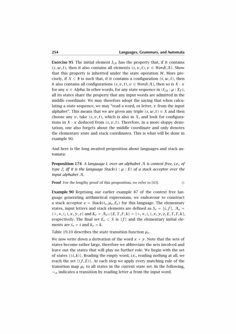
254 Languages, Grammars, and Automata
Exercise 95 The initial element Ii,k has the property that, if it contains
(s,w, t), then it also contains all elements (s, v, t), v ∈ Word(A). Show
that this property is inherited under the state operation M . More pre-
cisely, if X ⊂ S is such that, it it contains a configuration (s,w, t), then
it also contains all configurations (s, v, t), v ∈ Word(A), then so is X · xfor any x ∈ Alpha. In other words, for any state sequence in (Ii,k : µ : EE),all its states share the property that any input words are admitted in the
middle coordinate. We may therefore adopt the saying that when calcu-
lating a state sequence, we may “read a word, or letter, v from the input
alphabet”. This means that we are given any triple (s,w, t) ∈ X and then
choose any v , take (s, v, t), which is also in X, and look for configura-
tions in X · x deduced from (s, v, t). Therefore, in a more sloppy deno-
tation, one also forgets about the middle coordinate and only denotes
the elementary state and stack coordinates. This is what will be done in
example 90.
And here is the long awaited proposition about languages and stack au-
tomata:
Proposition 174 A language L over an alphabet A is context free, i.e., of
type 2, iff it is the language Stack(i : µ : E) of a stack acceptor over the
input alphabetA.
Proof For the lengthy proof of this proposition, we refer to [43]. �
Example 90 Reprising our earlier example 87 of the context free lan-
guage generating arithmetical expressions, we endeavour to construct
a stack acceptor e = Stack(ie, µe, Ee) for this language. The elementary
states, input letters and stack elements are defined as Se = {i, f}, Ae ={+,∗, (, ), x,y, z} and Ke =Ae∪{E, T , F, k} = {+,∗, (, ), x,y, z, E, T , F, k},respectively. The final set Ee ⊂ S is {f} and the elementary initial ele-
ments are ie = i and ke = k.
Table 19.10 describes the state transition function µe.
We now write down a derivation of the word x + y . Note that the sets of
states become rather large, therefore we abbreviate the sets involved and
leave out the states that will play no further role. We begin with the set
of states {(i, k)}. Reading the empty word, i.e., reading nothing at all, we
reach the set {(f , E)}. At each step we apply every matching rule of the
transition map µe to all states in the current state set. In the following,
→a indicates a transition by reading letter a from the input word.
19.3 Automata and Acceptors 255
Se ×Aeε ×Ke -→µe 2S×Word(K)
(i, ε,k) {(f , E )}(f , ε,E) {(f , T + E ), (f ,T)}(f , ε,T) {(f , F ∗ E ), (f , F)}(f , ε, F) {(f , (E) ), (f , x), (f ,y), (f , z)}(f , x, x) {(f , ε)}(f ,y,y) {(f , ε)}(f , z, z) {(f , ε)}(f ,+,+) {(f , ε)}(f ,∗,∗) {(f , ε)}(f , ( , ( ) {(f , ε)}(f , ) , ) ) {(f , ε)}
Fig. 19.10. The transition map µe for the stack acceptor of example 90.
{(i, k)} →ε {(f , E)}→ε {(f , T + E), (f , T)}→ε {(f , F ∗ E + E), (f , F ∗ E), (f , F + E), (f , F)}→ε {. . . , (f , x + E), . . .}→x {. . . , (f ,+E), . . .}→+ {. . . , (f , E), . . .}→ε {. . . , (f , T + E), (f , T), . . .}→ε {. . . , (f , F ∗ E + E), (f , F ∗ E), (f , F + E), (f , F), . . .}→ε {. . . , (f ,y), . . .}→y {. . . , (f , ε), . . .}
In the final line, the current set of states includes a state (f , ε) which
satisfies the conditions of a final state, Ee being {f} and the stack word
being empty.
Note how the form of a rule (s, a, k) → (s, k1k) justifies the image of
“push”, k1 being pushed on top of k. In the same way a rule (s, a, k) →(s, ε) “pop”s off k.
We leave it to the reader to compare the map µe with the set of grammar
rules in example 87 and to find out how they relate.
256 Languages, Grammars, and Automata
19.3.2 Turing Machines
Intuitively, Turing machines—named after the mathematician Alan Tur-
ing (1912–1954), one of the founders of computer science—are finite au-
tomata which are provided with an infinite tape memory and sequen-
tial access using a read/write head. We shall give a formal definition be-
low, but we should make a point concerning the general formalism of
automata and the concrete technical setup where particular types of au-
tomata are realized. We had in fact already learned above that stack ac-
ceptors are acceptors which are defined by auxiliary operations on com-
plex spaces. The same is true for Turing machines.
For Turing machines, one is essentially given a state set S, a tape alphabet
B which includes a special sign # for a “blank” entry on a specific place on
the tape. The tape is thought to be infinite to the left and to the right of
the read/write head. On the tape, we may have any elements of B, except
that only finitely many differ from #. The set of tape states is therefore
described by the subset B(Z) of BZ of those sequences t = (ti), ti ∈ Bwith ti = # for all but finitely many indexes i ∈ Z (mathematicians often
say in this case: “for almost all indexes”). The read/write head position
is by definition the one with index i = 0. With this vocabulary, a Turing
machine, as we shall define shortly, yields a map
τ : S × B(Z) → 2S×B(Z),
which describes the transition from one pair “state s of automaton plus
tape state t” to a set of possible new pairs s′ and t′ of the same type.
The machine continues updating states and tape until it reaches a “halt”
state. This looks somewhat different from the definition of an automa-
ton, which requires a map S × A → S. However, this formalism is also
present in the previous description. One must in fact use the natural ad-
junction of set maps discussed in proposition 59: The sets Set(a × b, c)and Set(a, cb) are in a natural bijection. Therefore
Ad : Set(S × B(Z),2S×B(Z)) ∼→ Set(S × B(Z) × B(Z),2S)
which means that the Turing automaton map τ corresponds to a map
Ad(τ) : S × (B(Z) × B(Z))→ 2S ,
19.3 Automata and Acceptors 257
and this is precisely the type of maps we need for automata, i.e., the al-
phabet isA= B(Z)×B(Z). We call the bijectionAd the Turing adjunction.5
The alphabetA happens to be infinite, but the formalism is the required
one. The meaning ofAd(τ) is this: We are given a present state s ∈ S and
a pair (t, t′) of tape states, t is the present tape state, whereas t′ is one of
the possible successor tape state. The set Ad(τ)(s, t, t′) is precisely the
set of those successor states s′ ∈ S such that (s′, t′) ∈ τ(s, t), i.e., which
correspond to the successor tape state t′.
But we shall stick to the original map τ in order to maintain the intuitive
setup. Here is the formal definition of Turing machines:
Definition 151 A Turing machine is given by
(i) a finite state set S, an initial state i ∈ S, and a special halt state sH
to be specified,
(ii) a finite tape alphabet B, containing a special blank sign #, together
with an input alphabetA⊂ B,
(iii) three symbols H,L,R not in B, one writes BHLR = {H,L,R} ∪ B,
(iv) a state transition map tr : S × B → 2S×BHLR with tr(s, b) ≠ ∅ for
all (s, b) ∈ S × B and such that only pairs (sH ,H) ∈ tr(s, b) may
appear with second coordinate H.
A Turing machine is deterministic iff every set tr(s, b) is a singleton, oth-
erwise it is called nondeterministic. The Turing machine is also denoted
by Turing(i, tr , sH), according to our general notation of acceptors.
This definition generates the following map τ. To begin with, the element
q ∈ BHLR of the extended tape alphabet operates on tape states t ∈ B(Z)as follows (we write q · t for the result of the operation of q on t):
1. if q ∈ B, then (q · t)i = ti for i ≠ 0, and (q · t)0 = q, i.e., the zero
position on the tape is replaced by q;
2. if q = H, nothing happens: q · t = t;3. if q = R, the tape moves one unit to the right, i.e., (q · t)i = ti−1;
4. if q = L, the tape moves one unit to the left, i.e., (q · t)i = ti+1.
5 Observe the omnipresence of universal constructions of mathematics in com-
puter science.

258 Languages, Grammars, and Automata
Then we have this map:
τ : S × B(Z) → 2S×B(Z)
τ(s, t) = {(s′, b′ · t) | (s′, b′) ∈ tr(s, t0)}
and the idea is that the change of states should go on until the halt state
sH is obtained. More precisely,
Definition 152 With the above notations, a state sequence of a Turing
machine Turing(i, tr, sH) is a sequence (s(0), t(0)), (s(1), t(1)), . . . (s(n), t(n))
such that (s(i+1), t(i+1)) ∈ τ(si, ti) for all indexes i = 0,1, . . . n− 1.
A word w = w1w2 . . .wk ∈ Word(A) is accepted by Turing(i, tr , sH) iff
there is a state sequence (s(0), t(0)), (s(1), t(1)), . . . (s(n), t(n)) which termi-
nates at the halt state, i.e., s(n) = sH , and starts at state s(0) = i and a tape
state t(0) with t(0)i = #, for i ≤ 0 and i > k, and t
(0)i = wi for i = 1,2, . . . k.
The language of words accepted by the Turing machine Turing(i, tr, sH)
is denoted by Turing(i : tr : sH). Languages of type Turing(i, tr, sH) for
given Turing machines are also called semi-decidable.
And here is the rewarding proposition relating Turing machines and type
0 languages:
Proposition 175 A language L ∈ Lang(A) is of type 0 (i.e., recursively
enumerable) iff it is semi-decidable, i.e., iff there is a Turing machine
Turing(i, tr , sH) with input alphabetA such that L = Turing(i : tr : sH).
Proof For the complicated proof of this proposition, we refer to [43]. �
Example 91 A simple example of an actual “program” for a Turing ma-
chine shall illustrate the principles of the foregoing discussion, and show
that Turing machines are capable of doing “useful” work, in this case
the incrementation of a natural number in binary representation, i.e.,
encoded using the symbols 0 and 1 on the initial tape state, where the
least-significant bit of the number is on the right of the tape. Thus the
number 151 will appear on the tape as . . .####10010111#### . . . . At the
beginning, the machine’s head will be at the position indicated by #. The
final tape state when the machine terminates in the halt state will be
. . .####10011000#### . . ., i.e., 152. Note that we use the Turing machine
a little differently than previously described. The object here is not to
accept an initial word, but to transform the initial word into the result
word.
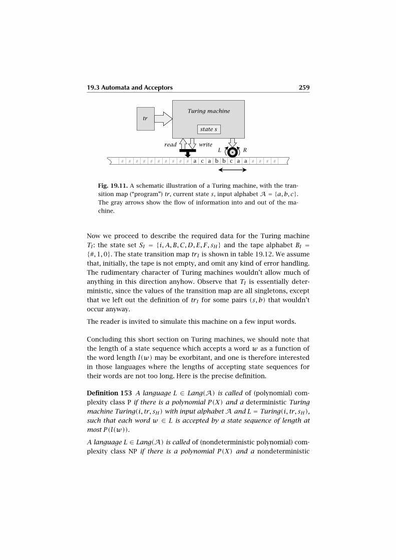
19.3 Automata and Acceptors 259
Fig. 19.11. A schematic illustration of a Turing machine, with the tran-
sition map (“program”) tr , current state s, input alphabet A = {a,b, c}.The gray arrows show the flow of information into and out of the ma-
chine.
Now we proceed to describe the required data for the Turing machine
TI : the state set SI = {i,A, B, C,D, E, F, sH} and the tape alphabet BI ={#,1,0}. The state transition map tr I is shown in table 19.12. We assume
that, initially, the tape is not empty, and omit any kind of error handling.
The rudimentary character of Turing machines wouldn’t allow much of
anything in this direction anyhow. Observe that TI is essentially deter-
ministic, since the values of the transition map are all singletons, except
that we left out the definition of tr I for some pairs (s, b) that wouldn’t
occur anyway.
The reader is invited to simulate this machine on a few input words.
Concluding this short section on Turing machines, we should note that
the length of a state sequence which accepts a word w as a function of
the word length l(w) may be exorbitant, and one is therefore interested
in those languages where the lengths of accepting state sequences for
their words are not too long. Here is the precise definition.
Definition 153 A language L ∈ Lang(A) is called of (polynomial) com-
plexity class P if there is a polynomial P(X) and a deterministic Turing
machine Turing(i, tr, sH) with input alphabetA and L = Turing(i, tr , sH),
such that each word w ∈ L is accepted by a state sequence of length at
most P(l(w)).
A language L ∈ Lang(A) is called of (nondeterministic polynomial) com-
plexity class NP if there is a polynomial P(X) and a nondeterministic
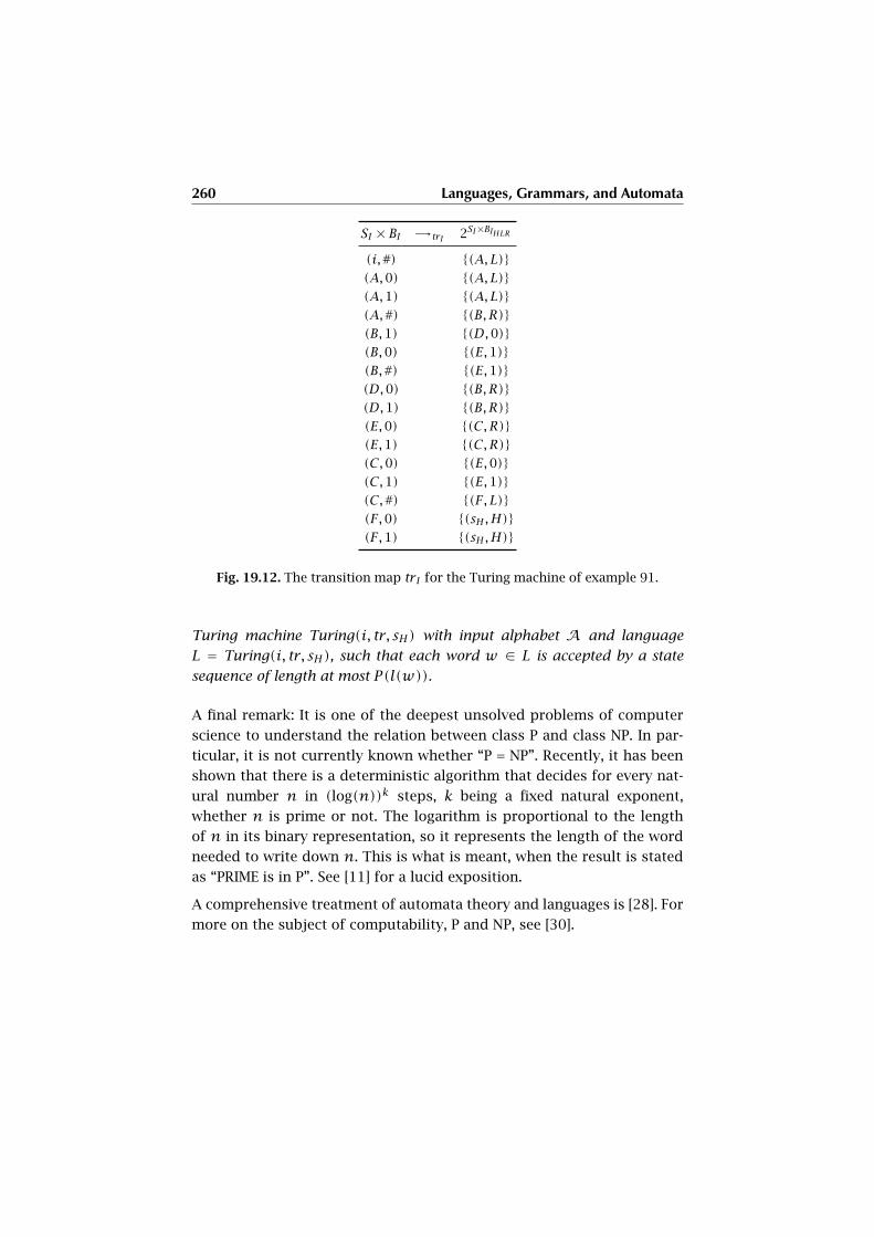
260 Languages, Grammars, and Automata
SI × BI -→trI 2SI×BIHLR
(i,#) {(A, L)}(A,0) {(A, L)}(A,1) {(A, L)}(A,#) {(B,R)}(B,1) {(D,0)}(B,0) {(E,1)}(B,#) {(E,1)}(D,0) {(B,R)}(D,1) {(B,R)}(E,0) {(C,R)}(E,1) {(C,R)}(C,0) {(E,0)}(C,1) {(E,1)}(C,#) {(F, L)}(F,0) {(sH ,H)}(F,1) {(sH ,H)}
Fig. 19.12. The transition map tr I for the Turing machine of example 91.
Turing machine Turing(i, tr, sH) with input alphabet A and language
L = Turing(i, tr , sH), such that each word w ∈ L is accepted by a state
sequence of length at most P(l(w)).
A final remark: It is one of the deepest unsolved problems of computer
science to understand the relation between class P and class NP. In par-
ticular, it is not currently known whether “P = NP”. Recently, it has been
shown that there is a deterministic algorithm that decides for every nat-
ural number n in (log(n))k steps, k being a fixed natural exponent,
whether n is prime or not. The logarithm is proportional to the length
of n in its binary representation, so it represents the length of the word
needed to write down n. This is what is meant, when the result is stated
as “PRIME is in P”. See [11] for a lucid exposition.
A comprehensive treatment of automata theory and languages is [28]. For
more on the subject of computability, P and NP, see [30].
CHAPTER 20
Categories of Matrixes
The present chapter opens a field of mathematics which is basic to all
applications, be it in equation solving, geometry, optimization, calculus,
or numerics. This field is called linear algebra. It is the part of algebra,
which we do control best—in contrast to non-linear algebra, also called
algebraic geometry, which is far more difficult. Linear algebra deals with
the structural theory of vectors, and the geometry they describe. We shall,
however, see later in the chapters on calculus that even non-linear, or—
worse than that—non-algebraic phenomena of continuous and infinites-
imal phenomena can in a first approximation be dealt with by linear al-
gebra. So here we enter one of the most powerful domains of mathe-
matics, and also one for which algorithms and corresponding computer
programs are most developed.
The structure of linear algebra rests on three pillars, which complement
each other, but are of equal importance for a real grasp of the subject:
Matrix theory, axiomatic theory of vector spaces, and linear geometry.
First, matrix theory is the calculatory backbone, it is nothing less than
the mathematical theory of tables. Without knowing the essentials about
matrixes, any understanding of arrays, lists, or vectors becomes difficult,
and no real, concrete calculation is possible. Strangely enough it turns out
that the system of matrixes is at the same time the most concrete and the
most abstract structure of this field. This is hinted at by attribute “cate-
gory” in our title, a specification which will become more and more clear
with the evolution of the student’s understanding of fundamental struc-
tures in mathematics. Recall that we have already added this attribute
in the context of graphs. It is remarkable that things seemingly so dis-
262 Categories of Matrixes
tant as graphs and tables turn out to be core instances of a common
substance: the structure of a category. Presently, this is a philosophical
allusion rather than hard mathematics. But it is a hint at the beauty of
mathematics that any reader should learn to feel in the course of this
curriculum.
Second, axiomatic vector space theory is the account to the fact that the
truths which are “hard coded” in matrix theory can be encountered in
much less concrete situations. These situations seem to be unrelated to
matrixes, but, when analyzed in view of their structural substance, re-
veal a fantastic kind of conceptual generalization of matrix calculus. This
effect provides very operational perspectives to seemingly abstract situ-
ations.
Last, linear geometry is a very traditional branch of geometry, which
can be traced back to to Descartes and his analytical geometry. If one
rephrases the structural substance of points, lines, surfaces, together
with their operations, metrical properties, and transformational behav-
ior, then it turns out that one gets what is essentially the theory of vector
spaces. And this gives the dry calculations of matrix theory and the ab-
stract manipulations of vector space theory a sensorial perspective which
is not only beautiful by itself, but in turn helps to understand abstract
phenomena of matrix theory in a revealing environment of geometric in-
tuition. We should however point out that the geometric intuition about
abstract truths is not the only one: the auditory intuition as cultivated by
the experience music is another sensorial image of abstract mathematical
truths which for a number of problems is even better suited to yield ev-
idence of “abstract artifacts” (or even what some scientific businessmen
call “abstract nonsense”).
20.1 What Matrixes Are
In this and the following sections of this chapter, the zero and unit of a
ring R will be denoted by 0 and 1, respectively, if the context is clear. For
any natural number n, we denote by [1, n] the set of natural numbers
between 1 and n, including the extremal values 1 and n. For n = 0, the
set [1,0] is the empty set.
Definition 154 Given a ring R and two natural numbers m and n, a ma-
trix of size m × n, or m × n-matrix, with coefficients in R is a triple
20.1 What Matrixes Are 263
(m,n, M : [1,m]× [1, n]→ R). For non-zero m and n, the value M(i, j),
which is also written as Mij , is called the coefficient of M at index pair ij;
the number i is called the row index, while j is called the column index.
If the number of rows m and the number of columns n are clear, M is
also denoted by (Mij). For a row number i the i-th row matrix in M is the
matrix Mi• of size 1 × n with (Mi•)1j = Mij . For a column number j the
j-th column matrix inM is the matrixM•j of sizem×1 with (M•j)i1 = Mij .The set of m × n-matrixes over R is denoted by Mm,n(R), while the set of
all matrixes, i.e., the disjoint union of all setsMm,n(R), is denoted byM(R).
Clearly, every ring homomorphism f : R → S between rings gives rise to
a map M(f ) : M(R) → M(S), which sends a matrix M = (Mij) ∈ M(R) to
the matrix f(M) = f ◦M ∈ M(S) with (f (M)ij) = (f (Mij)), and which
therefore also sends Mm,n(R) into Mm,n(S).
Example 92 There is a number of special matrixes:
• The unique matrix for either m or n equal to 0 is denoted by 0�n,
m�0, or 0�0, respectively.
• If m = n, the matrix is called a square matrix.
• The following convention is very useful in matrix calculus: If i and j
are two natural numbers, the Kronecker delta symbol is the number
δij =
1 ∈ R if i = j,0 ∈ R if i ≠ j.
Then the square n× n-matrix defined by En = (δij) is called the unit
matrix of rank n—including the unique matrix 0�0 as a “degenerate”
special case.
• Also important are the so-called elementary matrixes. Given an index
pair ij, the number of rows m and the number of columns n, the
elementarym×n-matrix for this datum is the matrix E(i, j) such that
(E(i, j))uv = 0 except for uv = ij, where we have (E(i, j))ij = 1 (see
also figure 20.1).
Usually, a matrix M is represented as a rectangular table, where the entry
on row i and column j is the matrix coefficient Mij . Here is the tabular
representation of one example of a 2× 3-matrix M over the ring R = Z of
integer numbers:
264 Categories of Matrixes
M =( −2 5 0
0 26 3
)
If we have the canonical ring homomorphism f = mod7 : Z → Z7, then
the image f(M) is equal to this matrix over Z7:
f(M) =(
mod7(−2) mod7(5) mod7(0)
mod7(0) mod7(26) mod7(3)
)
One also writesM ≡ N mod d ifM,N ∈Mm,n(Z) and their images under
the canonical homomorphism modd : Z→ Zd coincide; so for example,
( −2 5 0
0 26 3
)≡(
5 5 0
0 5 3
)mod 7.
Or else, consider the 4× 3-matrix
M =
3.5+ i · 4 −i 4+ i · √5
−0.5 0 4− i · 2
i · 20 1 3.78− i0 −i −5− i · √3
with complex coefficients. We have the field automorphism of conjuga-
tion f(z) = z, which gives us the conjugate matrix
f(M) =M =
3.5+ i · 4 −i 4+ i · √5
−0.5 0 4− i · 2
i · 20 1 3.78− i0 −i −5− i · √3
=
3.5− i · 4 i 4− i · √5
−0.5 0 4+ i · 2
−i · 20 1 3.78+ i0 i −5+ i · √3
.
A third example comes closer to tables in common usage: word process-
ing environments. Suppose that we are given an alphabet C, which, to
be concrete, denotes the letters in the Courier font, whereas S denotes
the alphabet of letters in the Old German Schwabacher font. In a com-
mon word processing software, a text may be converted from Courier to
Schwabacher, more formally, we have a map γ : C → S. By the universal
property of monoids (proposition 111) and monoid algebras (proposi-
tion 120), the map γ induces a ring homomorphism
20.2 Standard Operations on Matrixes 265
f = IdZ〈Word(γ)〉 : Z〈Word(C)〉 → Z〈Word(S)〉,
which we may now apply to a table with Courier-typed text, i.e., elements
from the ring Z〈Word(C)〉, in order to obtain a table with text in the
Schwabacher font, i.e., elements from the ring Z〈Word(S)〉. For example,
if
M =(Author: ShakespeareWork: Hamlet
)
then
f(M) =( )
Definition 155 For any ring R, the transposition is the map
?τ : M(R)→M(R)
defined by (Mτ)ij = Mji for all index pairs ij, thereby transforming a
m×n-matrix M into a n×m-matrix Mτ . A matrix M is called symmetric
if Mτ = M .
Exercise 96 For any natural number n, the identity matrix En is sym-
metric. If E(i, j) is elementary, then E(i, j)τ = E(j, i). Show that for any
matrix M , we have
(Mτ)τ = M.In particular, matrix transposition is a bijection on the set M(R).
E3 =
1 0 0
0 1 0
0 0 1
E(2,3) =
0 0 0
0 0 1
0 0 0
E(3,2) =
0 0 0
0 0 0
0 1 0
Fig. 20.1. The unit matrix and the elementary matrixes E(2,3) and
E(3,2) = E(2,3)τ in M3,3.
20.2 Standard Operations on Matrixes
We now proceed to the algebraic standard operations on matrixes. We
now tacitly assume that the underlying ring R for M(R) is commutative,
and we shall explicitly state any deviation from this general assumption.
266 Categories of Matrixes
Definition 156 Given two matrixes M,N ∈ Mm,n(R), their sum M +N ∈Mm,n(R) is defined as follows: If one of the numbers m or n is 0, then
there is only one matrix in Mm,n(R), and we set M + N = m�n. Else, we
set (M +N)ij = Mij +Nij .
Sorite 176 With the addition defined in definition 156, the set Mm,n(R)
becomes an abelian group. For m or n equal to 0, this is the trivial (zero)
group. In the general case, the neutral element of Mm,n(R) is the zero
matrix 0 = (0), whereas the additive inverse −M is defined by (−M)ij =−Mij .
Exercise 97 Give a proof of sorite 176.
Definition 157 Given a matrix M ∈ Mm,n(R), and a scalar λ ∈ R, the
scalar multiplication λ·M is defined as follows: If one of the numbersm or
n is 0, then there is only one matrix in Mm,n(R), and we set λ ·M =m�n.
Otherwise we set (λ ·M)ij = λ ·Mij . The matrix λ ·M is also called “M
scaled by λ.”
In other words, as is the case with ring homomorphisms and addition,
scalar multiplication proceeds coefficient-wise, i.e., by operating on each
coefficient of the involved matrixes.
Sorite 177 With the definitions 156 and 157 of addition and scalar multi-
plication, we have these properties for any λ, µ ∈ R and M,N ∈Mm,n(R):
(i) Scalar multiplication is homogeneous, i.e., we have λ · (µ · M) =(λ · µ) ·M , therefore we may write λ · µ ·M for this expression.
(ii) Scalar multiplication is distributive, i.e., we have
(λ+ µ) ·M = λ ·M + µ ·M
and
λ · (M +N) = λ ·M + λ ·N.
(iii) Scalar multiplication and transposition commute: (λ ·M)τ = λ ·Mτ .
Exercise 98 Give a proof of sorite 177.
Proposition 178 Given positive row and column numbersm and n, every
matrix M ∈Mm,n(R) can be uniquely represented as a sum
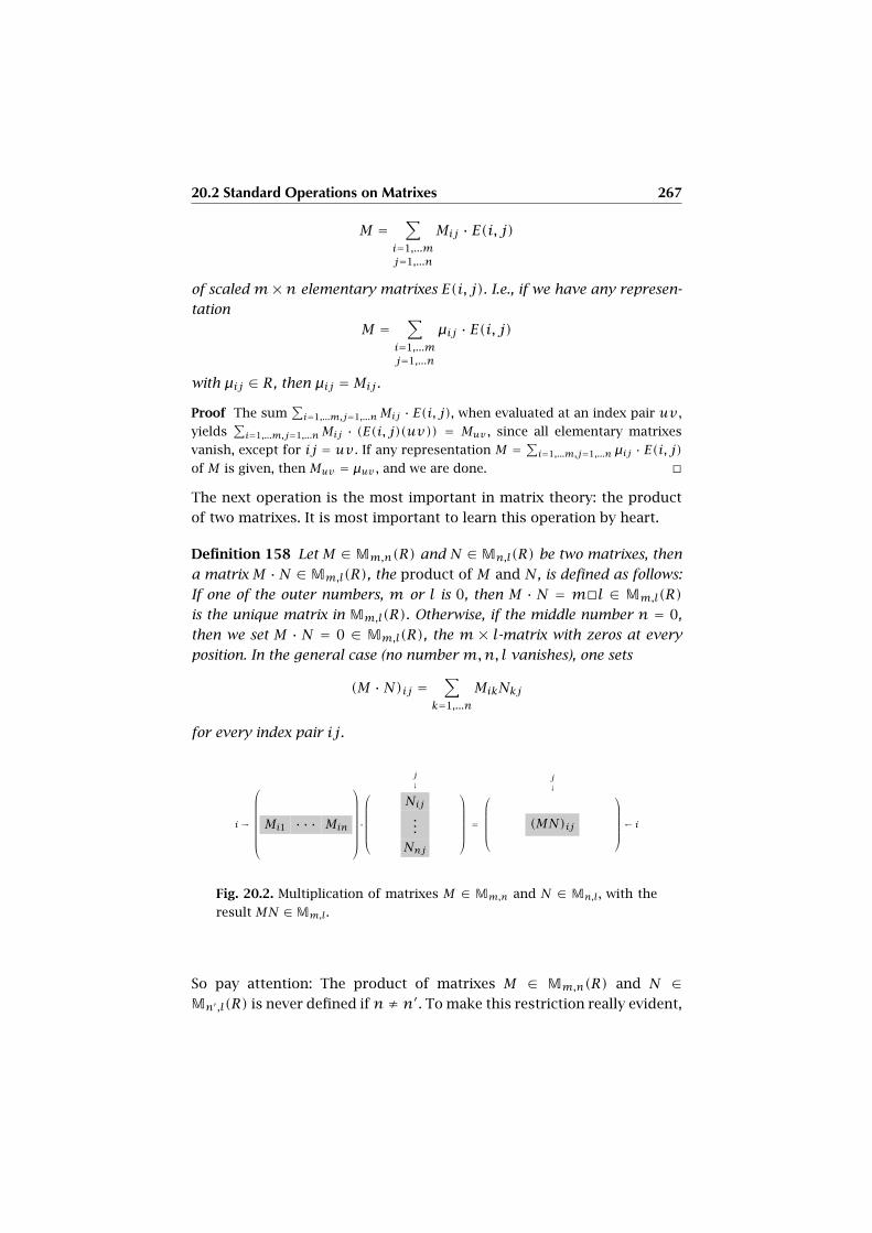
20.2 Standard Operations on Matrixes 267
M =∑
i=1,...mj=1,...n
Mij · E(i, j)
of scaledm×n elementary matrixes E(i, j). I.e., if we have any represen-
tation
M =∑
i=1,...mj=1,...n
µij · E(i, j)
with µij ∈ R, then µij = Mij .Proof The sum
∑i=1,...m,j=1,...nMij · E(i, j), when evaluated at an index pair uv ,
yields∑i=1,...m,j=1,...nMij · (E(i, j)(uv)) = Muv , since all elementary matrixes
vanish, except for ij = uv . If any representation M = ∑i=1,...m,j=1,...n µij · E(i, j)of M is given, then Muv = µuv , and we are done. �
The next operation is the most important in matrix theory: the product
of two matrixes. It is most important to learn this operation by heart.
Definition 158 Let M ∈Mm,n(R) and N ∈Mn,l(R) be two matrixes, then
a matrix M ·N ∈Mm,l(R), the product of M and N, is defined as follows:
If one of the outer numbers, m or l is 0, then M · N = m�l ∈ Mm,l(R)
is the unique matrix in Mm,l(R). Otherwise, if the middle number n = 0,
then we set M · N = 0 ∈ Mm,l(R), the m × l-matrix with zeros at every
position. In the general case (no number m,n, l vanishes), one sets
(M ·N)ij =∑
k=1,...n
MikNkj
for every index pair ij.
i→
Mi1 · · · Min
·
j
↓
Nij...
Nnj
=
j
↓
(MN)ij
← i
Fig. 20.2. Multiplication of matrixes M ∈ Mm,n and N ∈ Mn,l, with the
result MN ∈Mm,l.
So pay attention: The product of matrixes M ∈ Mm,n(R) and N ∈Mn′,l(R) is never defined if n ≠ n′. To make this restriction really evident,
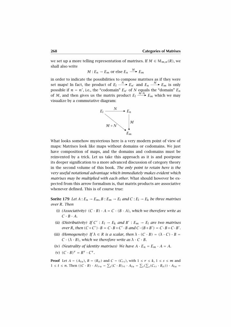
268 Categories of Matrixes
we set up a more telling representation of matrixes. If M ∈Mm,n(R), we
shall also write
M : En → Em or else EnMñ Em
in order to indicate the possibilities to compose matrixes as if they were
set maps! In fact, the product of ElNñ En′ and En
Mñ Em is only
possible if n = n′, i.e., the “codomain” En′ of N equals the “domain” Enof M , and then gives us the matrix product El
M·Nñ Em which we may
visualize by a commutative diagram:
ElN
ñ En
Em
M
�
M ◦Nñ
What looks somehow mysterious here is a very modern point of view of
maps: Matrixes look like maps without domains or codomains. We just
have composition of maps, and the domains and codomains must be
reinvented by a trick. Let us take this approach as it is and postpone
its deeper signification to a more advanced discussion of category theory
in the second volume of this book. The only point to retain here is the
very useful notational advantage which immediately makes evident which
matrixes may be multiplied with each other. What should however be ex-
pected from this arrow formalism is, that matrix products are associative
whenever defined. This is of course true:
Sorite 179 Let A : En → Em, B : Em → El and C : El → Ek be three matrixes
over R. Then
(i) (Associativity) (C · B) ·A = C · (B ·A), which we therefore write as
C · B ·A.
(ii) (Distributivity) If C ′ : El → Ek and B′ : Em → El are two matrixes
over R, then (C+C′)·B = C ·B+C′·B and C ·(B+B′) = C ·B+C ·B′.(iii) (Homogeneity) If λ ∈ R is a scalar, then λ · (C · B) = (λ · C) · B =
C · (λ · B), which we therefore write as λ · C · B.
(iv) (Neutrality of identity matrixes) We have A · En = Em ·A = A.
(v) (C · B)τ = Bτ · Cτ .
Proof Let A = (Atu), B = (Bst) and C = (Crs), with 1 ≤ r ≤ k, 1 ≤ s ≤ m and
1 ≤ t ≤ n. Then ((C · B) · A)ru =∑t(C · B)rt · Atu =
∑t(∑s(Crs · Bst)) · Atu =
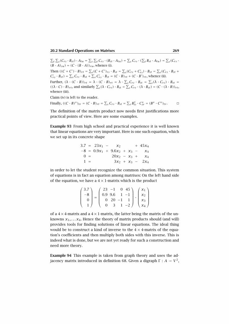
20.2 Standard Operations on Matrixes 269
∑t
∑s(Crs ·Bst) ·Atu =
∑s
∑t Crs · (Bst ·Atu) =
∑s Crs · (
∑t Bst ·Atu) =
∑s(Crs ·
(B ·A)su) = (C · (B ·A))ru, whence (i).
Then ((C + C′) · B)rt =∑s(C + C′)rs · Bst =
∑s(Crs + C′rs) · Bst =
∑s(Crs · Bst +
C′rs · Bst) =∑s Crs · Bst +
∑s C
′rs · Bst = (C · B)rt + (C · B′)rt , whence (ii).
Further, (λ · (C · B))rt = λ · (C · B)rt = λ ·∑s Crs · Bst =
∑s(λ · Crs) · Bst =
((λ · C) · B)rt , and similarly∑s(λ · Crs) · Bst =
∑s Crs · (λ · Bst) = (C · (λ · B))rt ,
whence (iii).
Claim (iv) is left to the reader.
Finally, ((C · B)τ)tr = (C · B)rt =∑s Crs · Bst =
∑s B
τts · Cτsr = (Bτ · Cτ)tr . �
The definition of the matrix product now needs first justifications more
practical points of view. Here are some examples.
Example 93 From high school and practical experience it is well known
that linear equations are very important. Here is one such equation, which
we set up in its concrete shape
3.7 = 23x1 − x2 + 45x4
−8 = 0.9x1 + 9.6x2 + x3 − x4
0 = 20x2 − x3 + x4
1 = 3x2 + x3 − 2x4
in order to let the student recognize the common situation. This system
of equations is in fact an equation among matrixes: On the left hand side
of the equation, we have a 4× 1-matrix which is the product
3.7
−8
0
1
=
23 −1 0 45
0.9 9.6 1 −1
0 20 −1 1
0 3 1 −2
·
x1
x2
x3
x4
of a 4×4-matrix and a 4×1-matrix, the latter being the matrix of the un-
knowns x1, . . . x4. Hence the theory of matrix products should (and will)
provides tools for finding solutions of linear equations. The ideal thing
would be to construct a kind of inverse to the 4 × 4-matrix of the equa-
tion’s coefficients and then multiply both sides with this inverse. This is
indeed what is done, but we are not yet ready for such a construction and
need more theory.
Example 94 This example is taken from graph theory and uses the ad-
jacency matrix introduced in definition 68. Given a digraph Γ : A → V 2,
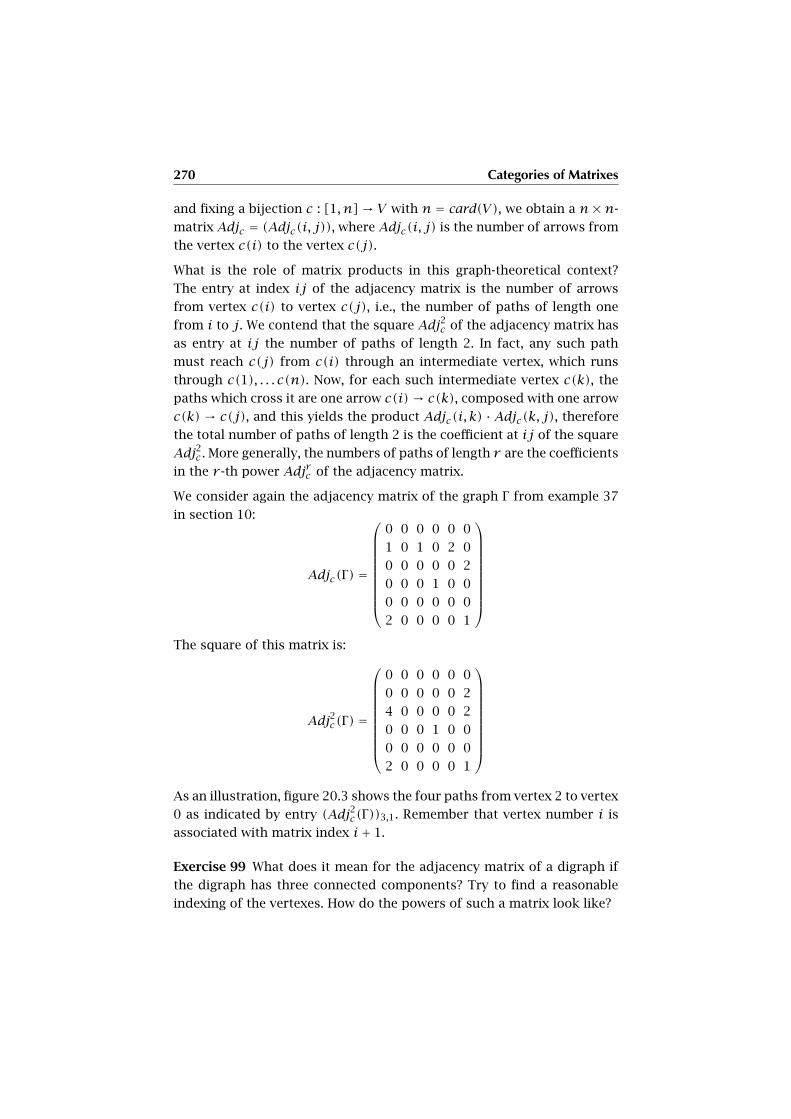
270 Categories of Matrixes
and fixing a bijection c : [1, n]→ V with n = card(V), we obtain a n×n-
matrix Adjc = (Adjc(i, j)), where Adjc(i, j) is the number of arrows from
the vertex c(i) to the vertex c(j).
What is the role of matrix products in this graph-theoretical context?
The entry at index ij of the adjacency matrix is the number of arrows
from vertex c(i) to vertex c(j), i.e., the number of paths of length one
from i to j. We contend that the square Adj2c of the adjacency matrix has
as entry at ij the number of paths of length 2. In fact, any such path
must reach c(j) from c(i) through an intermediate vertex, which runs
through c(1), . . . c(n). Now, for each such intermediate vertex c(k), the
paths which cross it are one arrow c(i)→ c(k), composed with one arrow
c(k) → c(j), and this yields the product Adjc(i, k) · Adjc(k, j), therefore
the total number of paths of length 2 is the coefficient at ij of the square
Adj2c . More generally, the numbers of paths of length r are the coefficients
in the r -th power Adjrc of the adjacency matrix.
We consider again the adjacency matrix of the graph Γ from example 37
in section 10:
Adjc(Γ) =
0 0 0 0 0 0
1 0 1 0 2 0
0 0 0 0 0 2
0 0 0 1 0 0
0 0 0 0 0 0
2 0 0 0 0 1
The square of this matrix is:
Adj2c(Γ) =
0 0 0 0 0 0
0 0 0 0 0 2
4 0 0 0 0 2
0 0 0 1 0 0
0 0 0 0 0 0
2 0 0 0 0 1
As an illustration, figure 20.3 shows the four paths from vertex 2 to vertex
0 as indicated by entry (Adj2c(Γ))3,1. Remember that vertex number i is
associated with matrix index i+ 1.
Exercise 99 What does it mean for the adjacency matrix of a digraph if
the digraph has three connected components? Try to find a reasonable
indexing of the vertexes. How do the powers of such a matrix look like?

20.3 Square Matrixes and their Determinant 271
Fig. 20.3. The four paths of length 2 from vertex 2 to vertex 0.
20.3 Square Matrixes and their Determinant
The most important matrixes are the square matrixes M of positive size
n, i.e., M ∈ Mn,n(R). We also tacitly assume R ≠ 0. We have this general
result to start with:
Proposition 180 Let n be a positive natural number and R a commuta-
tive, non-zero ring. Then the setMn,n(R), together with the sum and prod-
uct of matrixes is a ring which is not commutative except for n = 1. The
homomorphism of rings ∆ : R → Mn,n(R) : r , r · En identifies R with
the diagonal matrixes of size n with Mii = r , and Mij = 0 for i ≠ j. We
therefore also identify r ∈ R with its diagonal matrix r ·En if no confusion
is likely. Then, we have r ·M = M · r for all M ∈ Mn,n(R); we say that
R commutes with all matrixes of size n. No other matrixes commute with
all of Mn,n(R).
Proof The proposition immediately follows from sorite 179, except for the last
statement. Suppose that a n × n-matrix N commutes with all of Mn,n(R). Then
it must commute with all elementary matrixes E(i, j). But N · E(i, j) has zeros
except in column j which is N•i, whereas the product E(i, j)·N has zeros except
in row i which is Nj•. So, at the intersection of this row and this column, we
have the equation Nii = Njj , whereas all other coefficients must vanish, whence
N = λ = λ · En. �
Definition 159 The group Mn,n(R)∗ of invertible matrixes of size n is
called the general linear group of size n and denoted by GLn(R). An in-
vertible matrix is also called regular.
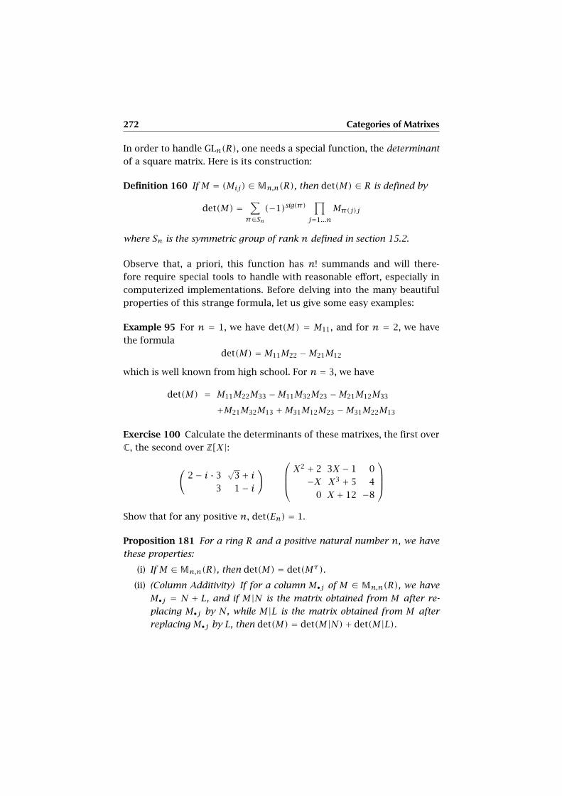
272 Categories of Matrixes
In order to handle GLn(R), one needs a special function, the determinant
of a square matrix. Here is its construction:
Definition 160 If M = (Mij) ∈Mn,n(R), then det(M) ∈ R is defined by
det(M) =∑
π∈Sn(−1)sig(π)
∏
j=1...n
Mπ(j)j
where Sn is the symmetric group of rank n defined in section 15.2.
Observe that, a priori, this function has n! summands and will there-
fore require special tools to handle with reasonable effort, especially in
computerized implementations. Before delving into the many beautiful
properties of this strange formula, let us give some easy examples:
Example 95 For n = 1, we have det(M) = M11, and for n = 2, we have
the formula
det(M) = M11M22 −M21M12
which is well known from high school. For n = 3, we have
det(M) = M11M22M33 −M11M32M23 −M21M12M33
+M21M32M13 +M31M12M23 −M31M22M13
Exercise 100 Calculate the determinants of these matrixes, the first over
C, the second over Z[X|:(
2− i · 3√
3+ i3 1− i
)X2 + 2 3X − 1 0
−X X3 + 5 4
0 X + 12 −8
Show that for any positive n, det(En) = 1.
Proposition 181 For a ring R and a positive natural number n, we have
these properties:
(i) If M ∈Mn,n(R), then det(M) = det(Mτ).
(ii) (Column Additivity) If for a column M•j of M ∈ Mn,n(R), we have
M•j = N + L, and if M|N is the matrix obtained from M after re-
placing M•j by N, while M|L is the matrix obtained from M after
replacing M•j by L, then det(M) = det(M|N)+ det(M|L).
20.3 Square Matrixes and their Determinant 273
(iii) (Row Additivity) If for a row Mi• of M ∈ Mn,n(R), we have Mi• =N+L, and ifM|N is the matrix obtained fromM after replacingMi•by N, while M|L is the matrix obtained from M after replacing Mi•by L, then det(M) = det(M|N)+ det(M|L).
(iv) (Column Homogeneity) If for a column M•j of M ∈ Mn,n(R), we
have M•j = λ · N, and if M|N is the matrix obtained from M after
replacing M•j by N, then det(M) = λ · det(M|N).(v) (Row Homogeneity) If for a rowMi• ofM ∈Mn,n(R), we haveMi• =λ ·N, and if M|N is the matrix obtained from M after replacing Mi•by N, then det(M) = λ · det(M|N).
(vi) (Column Skew Symmetry) If M ′ is obtained from M ∈ Mn,n(R)
by exchanging two columns M•j ,M•k, with j ≠ k, then det(M ′) =−det(M).
(vii) (Row Skew Symmetry) If M ′ is obtained from M ∈ Mn,n(R) by ex-
changing two rows Mi•,Mk•, with i ≠ k, then det(M ′) = −det(M).
(viii) (Column Equality Annihilation) If in M ∈ Mn,n(R), we have two
equal columns M•j = M•k with j ≠ k, then det(M) = 0.
(ix) (Row Equality Annihilation) If in M ∈ Mn,n(R), we have two equal
rows Mi• = Mk• with i ≠ k, then det(M) = 0.
(x) (Uniqueness of Determinant) Any function D : Mn,n(R) → R with
properties (ii), (iv), (viii) is uniquely determined by its value D(En),
and then we have D(M) = D(En) · det(M).
(xi) (Product Rule for Determinants) If M,N ∈Mn,n(R), then
det(M ·N) = det(M) · det(N).
(xii) (General Linear Group Homomorphism) The determinant function
induces a homomorphism
det : GLn(R)→ R∗
onto the multiplicative group R∗ of invertible elements of R. Its ker-
nel is denoted by SLn(R) and called the special linear group of size
n, whence GLn(R)/SLn(R)∼→ R∗.
(xiii) (Invariance under Conjugation) If M ∈ Mn,n(R) and C ∈ GLn(R),
then
det(C ·M · C−1) = det(M),
the matrix C ·M · C−1 being called the C-conjugate of M .1
1 Do not confuse matrix conjugation with the conjugation of a complex number.

274 Categories of Matrixes
Proof We have
det(M) =∑
π∈Sn(−1)sig(π)
∏
j=1...n
Mπ(j)j
=∑
π∈Sn(−1)sig(π)
∏
π(j)=1...n
Mπ(j)π−1(π(j))
=∑
π∈Sn(−1)sig(π)
∏
j=1...n
Mjπ−1(j)
=∑
π∈Sn(−1)sig(π)
∏
j=1...n
Mjπ(j)
=∑
π∈Sn(−1)sig(π)
∏
j=1...n
Mτπ(j)j
= det(Mτ),
whence (i).
If we have Mij = Ni + Li, for all i, then for each product in the determinant
function, we have∏
t=1...n
Mπ(t)t = Mπ(j)j∏
t≠j
Mπ(t)t
= Nπ(j)∏
t≠j
Mπ(t)t + Lπ(j)∏
t≠j
Mπ(t)t
= (M|N)π(j)j∏
t≠j
Mπ(t)t + (M|L)π(j)j∏
t≠j
Mπ(t)t
= (M|N)π(j)j∏
t≠j
(M|N)π(t)t + (M|L)π(j)j∏
t≠j
(M|N)π(t)t
=∏
t
(M|N)π(t)t +∏
t
(M|L)π(t)t
whence (ii).
To prove (iii), we use (ii) because of (i).
For column homogeneity (iv), we observe that∏
t
Mπ(t)t = Mπ(j)j∏
t≠j
Mπ(t)t
= λ(Nπ(j)∏
t≠j
Mπ(t)t)
=∏
t
(M|N)π(t)t .
Row homogeneity (v) follows from (iv) and (i).
Suppose that (viii) is true. Then (vi) follows immediately. In fact, take a matrix
M and two column indexes k and j. Take the new matrix M ′ which is derived
from M by adding column M•k to column M•j and adding M•j to column M•k.Then by (viii), det(M ′) = 0. But by (iii), 0 = det(M ′) = det(M|k|k)+ det(M|j|j)+
20.3 Square Matrixes and their Determinant 275
det(M|j|k)+ det(M), where M|k|k is the matrix derived from M , where we have
the k-th column M•k at column positions k, j, and M|j|j is the matrix derived
from M , where we have the j-th column M•j at column positions k and j, while
M|j|k is the matrix where the k-th and j-th columns of M have been exchanged.
But by (viii)det(M|k|k) = det(M|j|j) = 0, whence det(M|j|k) = −det(M). Also,
by (i) and (vi), (vii) follows.
To prove (viii), recall that the number of even permutations is n!/2 and that for
each even permutation π there is an odd permutation π∗ = (π(k),π(j)) ◦ π .
This gives us a bijection from even to odd permutations. But then, the product∏tMπ(t)t is equal to the product
∏tMπ∗(t)t since both columns at positions k
and j are equal. So by the change of signs, i.e., (−1)π∗ = −(−1)π , these products
neutralize each other. Further, by (i) and (viii), (ix) follows.
Claim (x) is demonstrated as follows: Each column is the sum of special columns
N, where only one coefficient Ni is possibly different from zero. So the function
D(M) is determined on matrixes having only one coefficient possibly different
from zero. But such a column N is also the scaling N = Ni · N′, where N′ has
coefficient 1 instead of Ni, and zeros else. So by homogeneity in columns, the
functionD is determined by its values on matrixes which have only columns with
a 1 and zero coefficients else. Now, by (viii), the value of our function D must
vanish if two columns are equal. If not, the matrix M results from a permutation
π of the columns of En, and the value must be D(M) = (−1)sig(π)D(En). Now,
sinceD(En)·det(M) has all the properties (ii),(iv),(viii) ofD, andD(En)·det(En) =D(En) we must have D(M) = D(En)det(M).
Suppose for (xi) that M,N ∈ Mn,n(R). Then, fixing M , the function D(N) =det(M · N) evidently has the properties (ii), (iv), and (viii) by the laws of matrix
multiplication. Since its value for N = En is det(M), we are done by (x). Further,
since by (xi) the determinant commutes with products of matrixes, it sends the
product En = M−1 ·M to 1 = det(M−1) · det(M), i.e., we have a group homomor-
phism GLn(R)→ R∗, which is surjective, since the matrixM = (λ−1)E(1,1)+Enhas det(M) = λ.
Claim (xii) follows from (xi) and the fact that det(En) = 1.
Claim (xiii) is evident from claim (xii). �
The calculation of the inverse of an invertible square matrix uses the
determinant function in a rather complex way. We first establish the nec-
essary auxiliary structures.
Definition 161 For positive n, we denote by iMj the (n − 1) × (n − 1)-
matrix derived from M ∈ Mn,n(R) by the cancellation of its i-th row and
j-th column. For n > 1, the determinant det(iMj) is called the ij-minor
of M . The number cof (M)ij = (−1)i+j det(jMi) is called the ij-cofactor of
276 Categories of Matrixes
M . The matrix Ad(M) = (cof (M)ij) ∈ M(R) is called the adjoint of M . If
n = 1, we set Ad(M) = E1.
Lemma 182 For a matrix M ∈ Mn,n(R), of size n > 1, if 1 ≤ i ≤ n is a
row index, then
det(M) =∑
j=1,...n
Mijcof (M)ji.
If 1 ≤ j ≤ n is a column index, then
det(M) =∑
i=1,...n
Mijcof (M)ji.
Proof We have
det(M) =∑
π∈Sn(−1)sig(π)
∏
t=1...n
Mπ(t)t
=∑
i=1,...n
Mij∑
π∈Sn,π(j)≠i(−1)sig(π)
∏
t≠j
Mπ(t)t .
The factor∑π∈Sn,π(j)≠i(−1)sig(π)
∏t≠jMπ(t)t is easily seen to be cof (M)ji, whence
the second formula. The first follows from the invariance of the determinant un-
der transposition. �
Proposition 183 (Cramer’s Rule) For a matrix M ∈ Mn,n(R), of positive
size n, we have the following equation:
M ·Ad(M) = det(M) · En.
Proof Cramer’s rule is an immediate consequence of lemma 182. If we take the
formula∑j=1,...nMijcof (M)ji and change the coefficient i to k ≠ i, then this is
the same formula for the matrix deduced from M , where the row at index i is
replaced by the row at index k. But such a matrix has determinant zero by row
equality annihilation (ix) in proposition 181. So the Cramer formula results. �
Proposition 184 A matrix M ∈Mn,n(R), of positive size n is invertible iff
det(M) ∈ R∗. In particular, if R is a field, this means that det(M) ≠ 0. If
M is invertible, then the inverse is given by this formula:
M−1 = 1
det(M)Ad(M).
Proof If M is invertible, we know that det(M) ∈ R∗. Conversely, if det(M) ∈ R∗,
then Cramer’s formula yields that the inverse is given by M−1 = 1det(M)Ad(M). �
20.3 Square Matrixes and their Determinant 277
Exercise 101 Decide whether the matrix
M =(
25 −1
12 5
)
over Z is invertible. Is its image M mod 12 over Z12 invertible? Try to
calculate the adjoint and, if M is invertible, the inverse matrix of M .
Exercise 102 Show that, if M ∈ Mn,n(R) is an upper triangular matrix,
i.e., Mij = 0 for all i > j, then det(M) =∏i=1...nMii.
Exercise 103 As a special case of matrix multiplications, we have already
mentioned linear equations, such as shown in example 93 above. We are
now in a position to solve such an equation
3.7
−8
0
1
=
23 −1 0 45
0.9 9.6 1 −1
0 20 −1 1
0 3 1 −2
·
x1
x2
x3
x4
.
In fact, if the coefficient matrix
23 −1 0 45
0.9 9.6 1 −1
0 20 −1 1
0 3 1 −2
is invertible, then the solution is
x1
x2
x3
x4
=
23 −1 0 45
0.9 9.6 1 −1
0 20 −1 1
0 3 1 −2
−1
.
3.7
−8
0
1
.
Proposition 185 If f : R → S is a ring homomorphism of commutative
rings, then for a matrix M ∈Mn,n(R) of positive size n > 0, we have
det(f (M)) = f(det(M)).
Proof We have det(f (M)) = det(f ((Mij))), but the determinant is a sum of
products of the images f(Mij), and since f is a ring homomorphism, we have
det(f ((Mij))) = f(det((Mij))). �
278 Categories of Matrixes
Proposition 186 (Cayley-Hamilton Theorem) If T is a commutative ring,
and if N ∈ Mn,n(T) for positive n, the characteristic polynomial of N is
the polynomial χN(X) = det(N − X · En) ∈ T[X], where En ∈ Mn,n(T) is
the unit matrix of size n over T , and X is an indeterminate. Then we have
the Cayley-Hamilton equation
χN(N) = 0 ∈Mn,n(T),
moreover,
χN(0) = det(N).
The coefficients of the characteristic polynomial are invariant under con-
jugation, i.e., if C ∈ GLn(T), then χN = χC·N·C−1 .
Proof Let R = T[X] be the polynomial algebra over the commutative ring T
with the indeterminate X. By the universal property of the polynomial algebra,
if N ∈Mn,n(T), we have a unique ring homomorphism f : R →Mn,n(T) defined
by X , N. Its image ring S is commutative, since the polynomial ring T[X] is
so. The ring S consists of all polynomials in N with coefficients in T . Therefore,
by proposition 185, det(f (M)) = f(det(M)) for any matrix M ∈ Mn,n(T[X]).
In particular, if M = N − X · En for N ∈ Mn,n(T) for the unit matrix En in
Mn,n(T), then det(M) = χN(X) ∈ T[X], and we have f(χN(X)) = χN(N). But
also f(χN(X)) = f(det(M)) = det(f (M)) = det(f (N−X ·En)) = det(N−N) = 0.
Therefore,
χN(N) = 0.
As for the invariance under conjugation, we have
χC·N·C−1 = det(C ·N · C−1 −X · En)= det(C ·N · C−1 −X · C · C−1)
= det(C · (N −X · En) · C−1)
= det(N −X · En)= χN .
�
Exercise 104 Calculate the characteristic polynomial χN for the matrix
N =( −1 0
2 3
)
over the integers. Verify the Cayley-Hamilton equation χN(N) = 0.

CHAPTER 21
Modules and Vector Spaces
If the matrixes are the backbones of linear algebra, here is the flesh: the
axiomatic theory of modules and vector spaces, which encompasses a
large variety of comparable structures. They will eventually be cast into
matrixes in many interesting cases. The setup is drawn from the historic
approach of René Descartes in his analytic geometry. In this chapter, we
shall again stick to commutative rings except when we explicitly state the
contrary.
Definition 162 Let R be a ring, then a left R-module is a triple (R,M,µ :
R ×M → M), where M is an additively written abelian group of so-called
vectors, and µ is the scalar multiplication, usually written as µ(r ,m) =r ·m if µ is clear, with these properties:
(i) We have 1 ·m =m, for all m ∈ M .
(ii) For all r , s ∈ R and m,n ∈ M , we have
(r + s) ·m = r ·m+ s ·mr · (m+n) = r ·m+ r ·nr · (s ·m) = (rs) ·m
Given an R-module M , a subgroup S ⊂ M is called a submodule of M , if
for each r ∈ R and s ∈ S, then r · s ∈ S. It is also an R-module on its own
right. If the ring R is a field, the module is called an R-vector space.
Exercise 105 Show that by statement (ii) of definition 162, one always
has 0 ·m = r · 0 = 0 in a module.
280 Modules and Vector Spaces
Example 96 In the course of the last chapter, we have encountered
plenty of modules: Each set M =Mm,n(R), together with the sum of ma-
trixes and the scalar multiplication by ring elements defined in sorite 177
is an R-module. In particular, we have zero modules M0,n(R), Mm,0(R),
M0,0(R), each consisting of a zero group and the only possible scalar
multiplication.
But the fundamental idea of defining matrixes as R-valued functions on
certain domains ([1,m] × [1, n] for matrixes) can easily be generalized:
Take any setD and consider the set RD of functions onD with values in R.
Then the addition f +g of f , g ∈ RD defined by (f +g)(d) = f(d)+g(d)and the scalar multiplication (r · f)(d) = r · f(d) for r ∈ R defines a
module, which generalizes the idea for matrixes.
The following important subset of RD is also a module under the same
addition and scalar multiplication: the set R(D) of functions f : D → R
such that f(d) = 0 except for at most a finite number of arguments. For
example, if we consider the monoid algebra R〈M〉 of a monoid M , this
is precisely R(M), and the sum of its elements is the one we just defined.
Moreover, the identification of R-elements r with the element r ·eM yields
the scalar multiplication r · f for elements f ∈ R〈M〉.This idea generalizes as follows: We may view R as an R-module over it-
self: The vectors are the elements of R, the sum is the given sum in R,
and the scalar multiplication is the ring multiplication. This module is of
course “isomorphic” to M1,1(R) (we shall define what a module isomor-
phism is in a few lines from here). It is called the free R-module of dimen-
sion one and denoted by RR, or simply by R if the context is clear. With
this special module in mind, suppose we are given a module M over R.
Then for any set D, we have the module M (D) whose elements f : D → Mvanish except for a finite set of arguments d, and where sum and scalar
multiplication are again defined point-wise, i.e., (f +g)(d) = f(d)+g(d)and (r ·f)(d) = r ·f(d). This module is called the direct sum of D copies
of M and usually denoted by M⊕D; in the special case where D = n is a
natural number, M⊕n is also written as Mn. We now recognize that part
of the structure of complex numbers C can be regarded as the module
R2. In fact, addition of complex numbers is the vector addition on R2,
whereas the multiplication of a real number r with a complex number z
plays the role of the scalar multiplication r · z. The special case M = RR
has been introduced above in the module R(D). We also recognize that
the matrix module Mm,n(R) identifies with R⊕[1,m]×[1,n].
Modules and Vector Spaces 281
If we are given a finite family (Mi)i=1,...n of R-modules, the Cartesian prod-
uctM1×. . .Mn is given a module structure as follows: Vector addition and
scalar multiplication are defined component-wise, i.e.,
(m1, . . .mn)+ (m′1, . . .m
′n) = (m1 +m′
1, . . .mn +m′n),
and
r · (m1, . . .mn) = (r ·m1, . . . r ·mn).
This module is denoted by⊕i=1,...nMi and is called the direct sum of the
modules M1, . . .Mn.
The following example is a very comfortable restatement of abelian
groups in terms of modules: Each abelian group M is automatically a
Z-module by the following scalar multiplication: One defines z · m =m+m + . . .m, z times, for z > 0, −((−z) ·m) for z < 0, and 0 ·m = 0.
Verify that this construction satisfies the module axioms.
Already after these first examples one recognizes that many modules are
manifestations of essentially the same structure. And this is why we once
more return to the principle of morphisms, after we already used it for
sets, digraphs, rings, and automata:
Definition 163 If (R,M,µ : R ×M → M) and (R,N, ν : R × N → N) are
two R-modules, an R-linear homomorphism f : M → N is a group homo-
morphism such that for all (r ,m) ∈ R ×M , f(µ(r ,m)) = ν(r , f (m)). If
no ambiguity about the scalar multiplications in M and in N is likely, one
uses the dot notation, and then linearity reads as f(r ·m) = r · f(m).The set of R-linear homomorphisms f : M → N is denoted by LinR(M,N).
By point-wise addition and scalar multiplication, LinR(M,N) is also pro-
vided with the structure of an R-module, which we henceforth tacitly as-
sume.
If L is a third R-module, the composition g ◦ f of two R-linear homomor-
phisms f ∈ LinR(M,N) and g ∈ LinR(N, L) is defined by their set-theoretic
composition; it is again R-linear.
For M = N, one writes EndR(M) = LinR(M,M) and calls its elements R-
module endomorphisms. In particular, the identity IdM : M → M is an
R-module endomorphism on M .
An R-linear homomorphism f : M → N is called an isomorphism if it has
an inverse g : N → M such that g ◦ f = IdM and f ◦ g = IdN . Evidently,

282 Modules and Vector Spaces
this is the case iff the underlying group homomorphism is a group iso-
morphism; the inverse is uniquely determined and denoted by g = f −1. If,
moreover, M = N, an isomorphism is called automorphism.
Exercise 106 Show that the matrix R-module Mm,n(R) is isomorphic
to Rmn. In particular, the column matrix module Mm,1(R) and the row
matrix module M1,m(R) are both isomorphic to Rm, and all modules
M0,n(R), Mm,0(R), M0,0(R) and R0 are isomorphic, i.e., they are trivial
R-modules.
Exercise 107 Show that the ring LinR(R,R) is isomorphic to R, in par-
ticular, observe that therefore these objects are also isomorphic as R-
modules.
Sorite 187 If f ∈ LinR(N, L) and g ∈ LinR(M,N), then
(i) if f = f1 + f2, then f ◦ g = (f1 + f2) ◦ g = f1 ◦ g + f2 ◦ g, whereas
for g = g1 + g2, f ◦ g = f ◦ (g1 + g2) = f ◦ g1 + f ◦ g2.
(ii) If r ∈ R, then r · (f ◦ g) = (r · f) ◦ g = f ◦ (r · g).(iii) With the addition and composition of linear endomorphisms on M ,
the set EndR(M) is a (generally not commutative) ring. If M ≠ 0,
R identifies with the subring R · IdM by the ring isomorphism R∼→
R · IdM : r , r · IdM , and it commutes with every endomorphism.
The group of invertible elements in EndR(M) is denoted by GL(M),
it is called the general linear group of M .
Proof Let g : M → N and f : N → L be R-linear homomorphisms. If f = f1 + f2,
then for x ∈ M , ((f1 + f2) ◦ g)(x) = (f1 + f2)(g(x)) = f1(g(x)) + f2(g(x)) =(f1 ◦ g)(x) + (f2 ◦ g)(x) = ((f1 ◦ g) + (f2 ◦ g))(x). If g = g1 + g2, then (f ◦(g1 + g2))(x) = f((g1 + g2)(x)) = f(g1(x) + g2(x)) = f(g1(x)) + f(g2(x)) =(f ◦ g1)(x)+ (f ◦ g2)(x) = ((f ◦ g1)+ (f ◦ g2))(x), whence (i).
If r ∈ R, then (r · (f ◦g))(x) = r · ((f ◦g)(x)) = r · (f (g(x)). But also ((r ·f)◦g)(x) = ((r · f)(g(x)) = r · f(g(x)). Finally (f ◦ (r · g))(x) = f((r · g)(x)) =f(r · g(x)) = r · f(g(x)), whence (ii).
Claim (iii) follows now immediately from (i) and (ii). �
Example 97 Consider the R-modulesMn,1(R) andMm,1(R) of n-element
and m-element columns. Then an m × n-matrix M : En → Em defines a
map fM : Mn,1(R)→Mm,1(R) by the matrix multiplication fM(X) = M ·X.
This gives us an a posteriori justification of the functional notation of a
Modules and Vector Spaces 283
matrix. The general laws of matrix multiplication stated in sorite 179 im-
ply that this map is R-linear. Moreover, applying fM to the elementary
column E(i,1) ∈ Mn,1(R) gives us the column Mi• of M . Therefore the
map M , fM is injective. We shall soon see that the map is often also
surjective, i.e., the matrixes are essentially the same thing as linear ho-
momorphisms! This is not always the case, but for a large class of rings,
the fields, and therefore for all vector spaces, this is true.
Analogous to groups, one can also build quotient and image modules as
follows:
Proposition 188 Given an R-linear homomorphism f : M → N, the image
group Im(f ) is a submodule of N. The kernel Ker(f ) of the underlying
group homomorphism is a submodule of M .
If S ⊂ M is a submodule of the R-module M , then the quotient group M/S
is also an R-module by the scalar multiplication r · (m + S) = r ·m + S.
This will be called the quotient R-module.
Proof The fact that Im(f ) and Ker(f ) are submodules is immediate and left
to the reader. If S ⊂ M is a submodule, then the scalar multiplication is well
defined, in fact, m+ S =m′ + S iff m−m′ ∈ S But then r ·m+ S = r ·m′ + Ssince r ·m − r ·m′ = r(m −m′) ∈ S. That this scalar multiplication satisfies
the module axioms is then immediate. �
And here is the universal property of quotient modules:
Proposition 189 Let M be an R-module and S ⊂ M a R-submodule of M .
Then for every R-module N, we have a bijection
LinR(M/S,N)∼→ {f | f ∈ LinR(M,N) and S ⊂ Ker(f )}.
Proof Let p : M → M/S be the canonical projection. If g : M/S → N is R-linear,
then the composition g◦p : M → N is in the set on the right hand side. Since p is
surjective, the map g , g ◦p is injective (see the characterization of surjections
of sets in sorite 16). Conversely, if f : M → N is such that S ⊂ Ker(f ), then we
may define a map g : M/S → N : m + S , f(m). Is this map well defined? If
m + S =m′ + S, then m −m′ ∈ S, hence f(m)− f(m′) = f(m −m′) = 0. It is
evidently R-linear, and we are done, since f = g ◦ p. �
Here is the (double) universal property of the finite direct sum:
Proposition 190 If M1, . . .Mn is a finite family of R-modules Mi, we have
R-linear injections ιj : Mj →⊕iMi : m , (0, . . .0,m,0, . . .0) for each
284 Modules and Vector Spaces
j = 1, . . . n, which map an element m ∈ Mj to the n-tuple having zeros
except at the j-th position, where the element m is placed. For any R-
module N, this defines a bijection
LinR(⊕
i
Mi, N)∼→⊕
i
LinR(Mi, N)
between sets of homomorphisms defined by f , (f ◦ ιi)i.Dually, we have R-linear projections πj :
⊕iMi → Mj : (mi)i , mj , for
each j = 1, . . . n. For any R-module N, this defines a bijection
LinR(N,⊕
i
Mi)∼→⊕
i
LinR(N,Mi)
between sets of homomorphisms defined by f , (πi ◦ f)i.Proof The isomorphisms f , (f ◦ ιi)i and f , (πi ◦ f)i indicated in the propo-
sition allow an immediate verification of the claims. We leave the details to the
reader. �
Exercise 108 Suppose we are given two subspaces U,V ⊂ M and con-
sider the homomorphism f : U ⊕ V → M guaranteed by proposition 190
and these two inclusions. Then show that f is an isomorphism iff (i)
U ∩ V = 0 and (ii) M = U + V , which means that every m ∈ M is a
sum m = u + v of u ∈ U and v ∈ V . In this case M is also called the
inner direct sum of U and V , and U and V are said to be complements to
each other.
Remark 25 If we consider the two injections iM : M → M ⊕ N and iN :
N → M ⊕ N, an element m ∈ M is mapped to iM(m) = (m,0), while
an element n ∈ N is mapped to iN(n) = (0, n). If it is clear from the
context that m belongs to the direct summand M and n to N, then one
also identifiesm with iM(m) and n to iN(n). With this identification, one
may add m to n and write m + n instead of iM(m) + iN(n). From now
on, this comfortable and economic notation will often be used without
special emphasis.
The following enables the reduction of linear algebra to matrix algebra
for a class of modules called free:
Definition 164 For a finite number n, an R-module M is called free of
dimension n if it is isomorphic to Rn.
Modules and Vector Spaces 285
Attention: for general rings, a module is not necessarily free. A very sim-
ple example is a finite abelian group, such as Zn, which, as a Z-module,
cannot be free since any free non-zero Z module is infinite. At present,
you cannot know whether the dimension of a free module is uniquely
determined. That it is in fact unique is shown by this result:
Proposition 191 If an R-module M is free of dimension n and free of di-
mensionm, then n =m, and this uniquely defined dimension is also called
dim(M).
Proof This follows from the properties of the determinant. Let f : Rn → Rm
be an R-linear isomorphism with n < m. Any element x = (x1, . . . xn) ∈ Rncan be written as x = ∑
i=1,...n xiei, where ei = (0, . . .0,1,0, . . .0) has 1 at the
i-th position. Then since every element y ∈ Rm is an image under f , it can
be written as y = ∑i xif(ei). Now, consider the unit matrix Em, for which
we have det(Em) = 1. By the above, we may write each row E(1, i) ∈ Rm as
E(1, j) = ∑i=1,...n x(j)if(ei), for x(j)i ∈ R, i.e., as a combination of less than m
row vectors f(ei), i = 1, . . . n. Therefore, by the properties of the determinant,
especially equal row annihilation, the determinant must vanish, a contradiction,
therefore n ≥m. A symmetric argument shows m ≥ n, whence the claim. �
Example 98 The free R-module Rš is called the real plane, and RÂs is
called the real three-dimensional space.
It will be shown in the course of the next chapter that every vector space
has a dimension.
Proposition 192 IfM is a free R-module of dimension n, and if N is a free
R-module of dimension m, then the R-module LinR(M,N) is isomorphic to
Mm,n(R), i.e., free of dimension mn.
Proof We may wlog suppose thatM = Rn and N = Rm. Then by proposition 190,
we have an R-linear isomorphism LinR(M,N)∼→ ⊕
i=1,...m,j=1,...n LinR(R,R), with
LinR(R,R)∼→ R, and therefore dim(LinR(M,N)) = n ·m. One now maps the
homomorphism f defined by the sequence (mij)i=1...m,j=1,...n ∈⊕i=1,...m,j=1,...n R
to the matrix Mf with (Mf )ij =mij . This map is evidently a linear bijection. �
We are now in the position to define the determinant of any linear endo-
morphism of a moduleM of dimension n by the following observation: If
we have a free R-module M of dimension n and a linear endomorphism
f : M → M , then, if u : M → Rn is an isomorphism, we may consider the
linear homomorphism u ◦ f ◦ u−1 : Rn → Rn. This corresponds to a ma-
trix Mf ,u ∈ Mn,n(R). If we take another isomorphism u′ : M → Rn, then

286 Modules and Vector Spaces
we have the corresponding matrix Mf ,u′ ∈Mn,n(R), and it easily follows
that
Mf ,u′ = (u′u−1) ·Mf ,u · (u′u−1)−1.
Therefore, the determinant of f , if defined by
det(f ) = det(Mf ,u)
is well defined by our previous result on conjugation of matrixes, see (xiii)
of theorem 181.
Free modules are therefore fairly transparent, since their theory seems to
reduce to matrix theory. However, we still have some unknown situations
even with this easy type of modules: For example, if f : Rn → Rm is an R-
linear map, what is the structure of Ker(f ) or Im(f )? Are these modules
free? In general, they are not, but again, for vector spaces, this is true.
This will be shown in the next chapter.
CHAPTER 22
Linear Dependence, Bases,
and Dimension
In practice, modules often do not occur as free constructions, but as sub-
spaces, more precisely: kernels or even quotient spaces related to linear
homomorphisms. For example, if we are given a matrix M ∈ Mm,n(R),
the corresponding linear homomorphism fM : Rn → Rm has a kernel
Ker(fM) which plays a crucial role in the theory of linear equations. A
linear equation is a matrix equation of this type:
y1
y2
...
ym
=
a11 a12 . . . a1n
a21 a22 . . . a2n
......
...
am1 am2 . . . amn
·
x1
x2
...
xn
where the matrixes (yi) and M = (aij) are given and one looks for the
unknown column matrix (xi). One reinterprets this equation by the linear
homomorphism fM : Rn → Rm associated with M . We are given an ele-
ment y = (y1, y2, . . . ym) ∈ Rm and look for the inverse image f−1M (y)
of y under fM . The solutions of the above equations are by definition the
elements x ∈ f−1M (y). So this solution space is structured as follows: If x
is a particular solution, the solution space is
f−1M (y) = x + Ker(fM).
This means that we have to deal with the following two problems: (1)
Deciding if there is at least one particular solution and possibly find it.
(2) Describing the kernel of fM .

288 Linear Dependence, Bases, and Dimension
22.1 Bases in Vector Spaces
To tackle these problems, we shall restrict our theory to vector spaces, i.e.,
module over fields R during the rest of our discussion of linear algebra.
Definition 165 A finite sequence (xi) = (x1, x2, . . . xk), k ≥ 1, of elements
xi ∈ M of an R-vector space M is called linearly independent if one of the
following equivalent properties holds:
(i) A linear combination∑i=1,...k λixi of the vectors xi equals 0 iff we
have λi = 0 for all scalars λi.
(ii) The R-linear homomorphism f : Rk → M defined by f(λ1, . . . λk) =∑i=1,...k λixi is injective, i.e., Ker(f ) = 0.
If (xi) is not linearly independent, the sequence is called linearly depen-
dent.
Exercise 109 Give a proof of the equivalence of the properties in defini-
tion 165.
Exercise 110 Show that a linearly independent sequence (xi) cannot
contain the zero vector, nor can it contain the same vector twice. If (xi)
is linearly independent, then so is every permutation of this sequence.
This means that linear independence is essentially a property of the un-
derlying set {xi, i = 1, . . . k} of vectors. However, there are many reasons
to keep the sequential order here and in the following definitions of gen-
erators and bases, as well.
Exercise 111 Show that in the real vector space R(N), every sequence
(ei)i=0,1,2,...k, k ≥ 1 with ei = (0, . . .0,1,0, . . .) having a 1 exactly in po-
sition i ∈ N and 0 else, is linearly independent.
Exercise 112 Show that in a free vector space Rn of dimension n, the
sequence (xi)i=1,2,...n of the vectors x = (1,1, . . . ,1,0,0 . . .0) whose com-
ponents are 1 up to and including the i-th coordinate, and 0 thereafter,
is linearly independent.
Exercise 113 Consider the Q-vector space R, defined by the usual addi-
tion of “vectors”, i.e., real numbers, and the usual scalar multiplication,
but restricted to rational scalars. Show that the two vectors 1 and√
2
22.1 Bases in Vector Spaces 289
are linearly independent over Q. Use the results of exercise 69 about the
irrationality of√
2.
Definition 166 A finite sequence (xi) = (x1, x2, . . . xk), k ≥ 1, of elements
xi ∈ M of an R-vector spaceM is said to generateM if one of the following
equivalent properties holds:
(i) The vector space M equals the subspace of all linear combinations∑i=1,...k λixi of the vectors xi (also called the space generated by
(xi)).
(ii) The R-linear homomorphism f : Rk → M defined by f(λ1, . . . λk) =∑i=1,...k λixi is surjective, i.e., Im(f ) = M .
A vector space M is called finitely generated if there is a finite sequence
(xi) = (x1, x2, . . . xk), k ≥ 1 of elements xi ∈ M which generates M .
Exercise 114 Give a proof of the equivalence of the properties in defini-
tion 166.
Exercise 115 Consider the R-vector spaceM = R[X, Y]/(X12, Y 12). Show
that it is generated by the images of XiY j ,0 ≤ i, j,≤ 11, in M .
Definition 167 A finite sequence (xi) = (x1, x2, . . . xk), k ≥ 1 of elements
xi ∈ M of an R-vector space M is called a basis of M iff it is linearly inde-
pendent and generates M . Equivalently, (xi) is a basis, iff the R-linear ho-
momorphism f : Rk → M : (λ1. . . . λk) ,∑i=1,...k λixi is an isomorphism.
Since by proposition 191, the dimension ofM is uniquely determined, every
basis of M must have the same number of elements, i.e., k = dim(M).
Remark 26 We have excluded the zero vector spaces here, because in
those no finite sequence (x1, . . . xk), k ≥ 1, can be linearly independent.
To complete the general terminology, one also says that the empty se-
quence is linearly independent, and that it forms a basis for a zero space,
but this is merely a convention.
Exercise 116 Show that in a free vector space Rn of dimension n, the
sequence (xi)i=1,2,...n of the vectors x = (1,1, . . . ,1,0,0 . . .0) whose com-
ponents are 1 up to and including the i-th coordinate, and 0 thereafter,
is a basis of Rn. Show that the elementary matrixes E(i, j) of Mm,n(R),
m,n > 0, form a basis of this vector space (R being any field).
Here is the guarantee that bases always exist:
290 Linear Dependence, Bases, and Dimension
Proposition 193 A vector space which is finitely generated has a basis,
more precisely, for every finite sequence (xi) of generators, there is a sub-
sequence which is a basis of M .
Proof Let (x1, . . . xk), k ≥ 1, be a generating sequence, then consider the first
xi ≠ 0 (if there is none, we have the case of a zero space, and the “empty ba-
sis” does the job). The one-element sequence (xi1) is linearly independent since
λ·xi1 = 0, with λ ≠ 0, implies λ−1 ·λ·xi1 = xi1 = 0, a contradiction. Suppose we
have found a subsequence (xi1 , xi2 , . . . xir ), i1 < i2 < . . . ir , of linearly indepen-
dent vectors of maximal length. Then this generates the space for the following
reason: If i is an index i1 < i < ir , then xi is linearly dependent on the vectors
xij , ij ≤ i, by construction. If i > ir , then there is a non-trivial linear combination
0 = µ · xi +∑j=1,...r xij by the maximality of our sequence. But then µ ≠ 0, oth-
erwise, we would have linear dependence of the maximal sequence. Therefore xiis contained in the space generated by the maximal sequence (xi1 , xi2 , . . . xir ),
and we are done. �
Here is the famous Steinitz exchange theorem, which guarantees that vec-
tor subspaces are always embedded in a distinct way:
Proposition 194 (Steinitz Exchange Theorem) If (y1, y2, . . . yl) is a se-
quence of linearly independent vectors in a finitely generated vector space
M , and if (x1, x2, . . . xk) is a basis of M (guaranteed by proposition 193),
then l ≤ k, and there is a (possibly empty) subsequence (xi1 , xi2 , . . . xik−l)
of (x1, x2, . . . xk) such that (y1, y2, . . . yl, xi1 , xi2 , . . . xik−l) is a basis of M .
Proof There is a representation y1 =∑i λixi. Since y1 ≠ 0, there is a t, such that
λt ≠ 0. Then xt is in the space generated by the sequence (y1, x1, . . . xt , . . . xr )
(refer to the footnote of page 182 for the notation). But this is again a ba-
sis, since it generates the whole space and it is linearly independent. In fact,
if 0 = µ · y1 +∑i=1,...t,...r λixi is a non-trivial linear combination, then neces-
sarily, µ ≠ 0, but then y1 also has a representation as a linear combination
without xt , so 0 = y1 − y1 would have a non-trivial representation by the ba-
sis, a contradiction! Therefore we have a new basis (y1, x1, . . . xt , . . . xr ). Sup-
pose now that we have found a new basis (y1, y2, . . . yr , xi1 , xi2 , . . . xik−l), r ≤ l.If r = l we are done, otherwise we may proceed as initially with y1, how-
ever, we must show that we can still eliminate one of the remaining xij . But
if yr+1 =∑e=1,...r µeye +
∑f=1,...k−r λfxif , then there must exist a λf0 ≠ 0, other-
wise, the y would be linearly dependent. So we may eliminate xif0 and we may
proceed until all y are integrated in the basis. �
Remark 27 The proof of the Steinitz theorem is quite algorithmic. Let
us sketch the procedure: Suppose that we can find a linear combination
22.1 Bases in Vector Spaces 291
yj =∑i=1,...k λjixi for each yj . Then, starting with y1, take the first non-
vanishing coefficient λ1i(1) in the sequence (λ1i), which exists since y1 is
not zero. Clearly, replacing xi(1) by y1 in the basis (xi) gives us a new
basis. Now, suppose that we have already replaced some xi by y1, . . . yr
and still have a basis. Now, yr+1 (if such a vector is left) is also a lin-
ear combination of these new basis elements. However, it is impossible
that all coefficients of the remaining xi vanish since then the (yj) would
not be linearly independent. So we may go on as in the beginning and re-
place one such xi whose coefficient is not zero. This procedure eventually
yields the new basis which contains all yj .
Corollary 195 If N is a subspace of a vector space M of dimension
dim(M), then N is also finitely generated and dim(N) ≤ dim(M), equality
holding iff N = M . Moreover, there is a subspace C ⊂ M complemen-
tary to N, i.e., the homomorphism N ⊕ C → M defined by the inclusions
C,N ⊂ M via the universal property of direct sums (proposition 190) is an
isomorphism; in other words, M is the inner direct sum of N and C (see
exercise 108).
Proof We first show that N has a basis. If N = 0, we are done. Otherwise we
take a maximal sequence (y1, . . . yr ) of linearly independent vectors in N. Then
r ≤ k by Steinitz. This must generate N, otherwise, let z ∈ N be a vector which
is not a linear combination of y1, . . . yr . Then evidently (y1, . . . yr , z) is linearly
independent, a contradiction. So let (y1, . . . yl) be a basis of N, and (x1, . . . xk) a
basis of M . Then, by Steinitz, l ≤ k. If N = M , then by uniqueness of dimension,
l = k. If l = k, we may replace all of (x1, . . . xk) by the basis elements y1, . . . yr ,
and therefore N = M .
To find a complement of N, take the space spanned by the k − l elements x of
the old basis in the basis (y1, y2, . . . yl, xi1 , xi2 , . . . xik−l). This is clearly a com-
plement. �
Remark 28 So we have this image in the case of finite-dimensional vector
spaces over a fixed field R: If we fix an isomorphism uM : M∼→ Rdim(M)
for each R-vector space M , we obtain an isomorphism
tuM ,uN : LinR(M,N)∼→Mdim(N),dim(M)(R)
defined by the conjugation f : M → N , uN◦f ◦(uM)−1 and the canonical
interpretation of linear maps Rn → Rm as matrixes. In this setup, if we
are given a second linear map g : N → L, dim(L) = l, then we have
tuM ,uL(g ◦ f) = tuN ,uL(g) · tuM ,uN (f ) and tuM ,uM (IdM) = Edim(M),

292 Linear Dependence, Bases, and Dimension
i.e., the matrix product commutes with the composition of linear maps.
This may be visualized by commutative diagrams:
MuM
ñ Rm � Em
NuN
ñ
f
ñ
Rn
t(f )
ñ
� En
Mt(f )
ñ
L
g ◦ f
�
uLñ
g
ð
Rl
t(g ◦ f)�
t(g)
ð
� El
Mt(g◦f)
�
Mt(g)
ð
We therefore have restated vector space structures in terms of matrixes,
as predicted. But what happens if we change the basis of a vector space
M? Let us discuss this for endomorphisms of M which we transform
into square matrixes in Mn,n(R) of size n = dim(M). Suppose we are
given two bases which induce the isomorphisms u,v : M∼→ Rn. Then
u ◦ v−1 : Rn∼→ Rn defines a matrix X such that we have
tv,v(f ) = X−1 · tu,u(f ) ·X,
i.e., conjugation with the base change matrix X gives us the second matrix
of f . In particular, if M = Rn, and if v = IdRn , then this formula gives us
the matrix of f when calculated in the matrix representation from the
new basis, whose elements are the column vectors of X. In other words:
Corollary 196 If we have a new basis (xi) of the vector space Rn given
in terms of a matrix C of columns C•i which correspond to xi, then the
representation of a linear map matrix f : Rn → Rn in terms of the basis
(xi) is C−1 · f · C.
We can now state the relation between the dimensions of the kernel and
the image of a linear map.
Corollary 197 Let f : M → N be a linear homomorphism defined on a
finite-dimensional R-vector space M (the vector space N need not be finite-
dimensional). Then we have
dim(M) = dim(Im(f ))+ dim(Ker(f )).
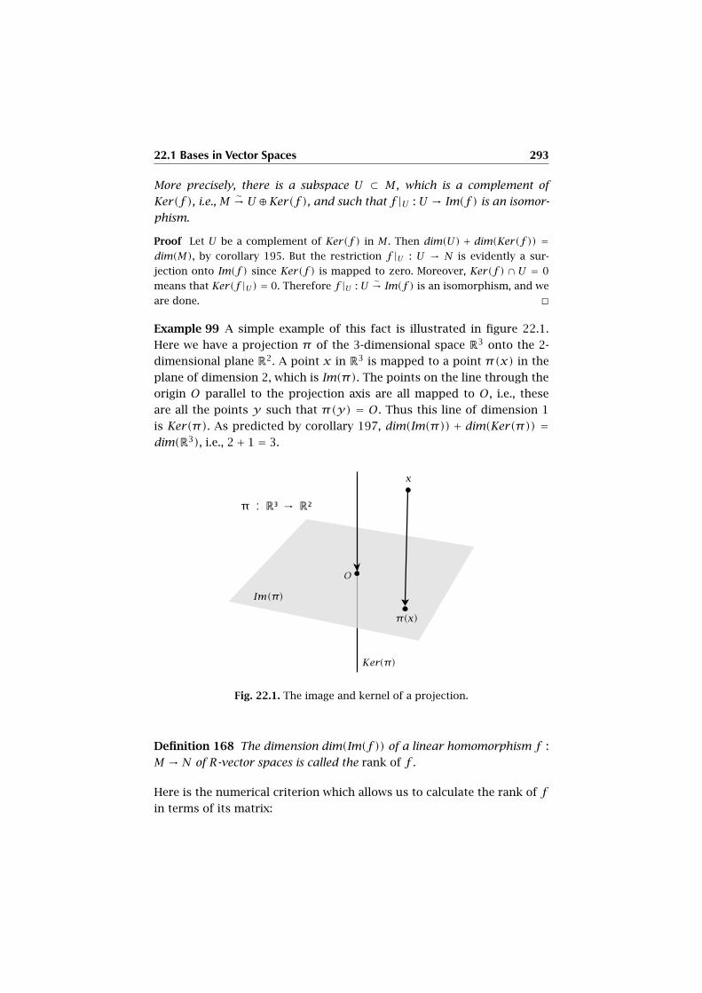
22.1 Bases in Vector Spaces 293
More precisely, there is a subspace U ⊂ M , which is a complement of
Ker(f ), i.e., M∼→ U ⊕Ker(f ), and such that f |U : U → Im(f ) is an isomor-
phism.
Proof Let U be a complement of Ker(f ) in M . Then dim(U) + dim(Ker(f )) =dim(M), by corollary 195. But the restriction f |U : U → N is evidently a sur-
jection onto Im(f ) since Ker(f ) is mapped to zero. Moreover, Ker(f ) ∩ U = 0
means that Ker(f |U) = 0. Therefore f |U : U∼→ Im(f ) is an isomorphism, and we
are done. �
Example 99 A simple example of this fact is illustrated in figure 22.1.
Here we have a projection π of the 3-dimensional space R3 onto the 2-
dimensional plane R2. A point x in R3 is mapped to a point π(x) in the
plane of dimension 2, which is Im(π). The points on the line through the
origin O parallel to the projection axis are all mapped to O, i.e., these
are all the points y such that π(y) = O. Thus this line of dimension 1
is Ker(π). As predicted by corollary 197, dim(Im(π)) + dim(Ker(π)) =dim(R3), i.e., 2+ 1 = 3.
Fig. 22.1. The image and kernel of a projection.
Definition 168 The dimension dim(Im(f )) of a linear homomorphism f :
M → N of R-vector spaces is called the rank of f .
Here is the numerical criterion which allows us to calculate the rank of f
in terms of its matrix:
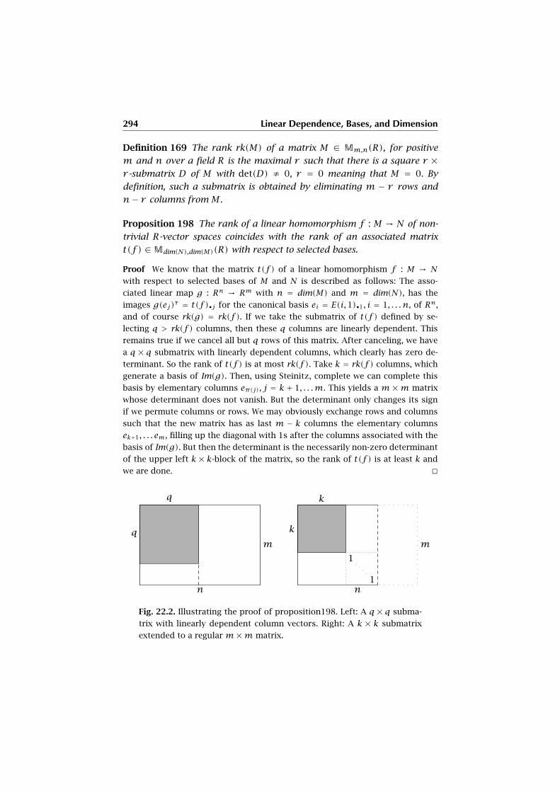
294 Linear Dependence, Bases, and Dimension
Definition 169 The rank rk(M) of a matrix M ∈ Mm,n(R), for positive
m and n over a field R is the maximal r such that there is a square r ×r -submatrix D of M with det(D) ≠ 0, r = 0 meaning that M = 0. By
definition, such a submatrix is obtained by eliminating m − r rows and
n− r columns from M .
Proposition 198 The rank of a linear homomorphism f : M → N of non-
trivial R-vector spaces coincides with the rank of an associated matrix
t(f ) ∈Mdim(N),dim(M)(R) with respect to selected bases.
Proof We know that the matrix t(f ) of a linear homomorphism f : M → N
with respect to selected bases of M and N is described as follows: The asso-
ciated linear map g : Rn → Rm with n = dim(M) and m = dim(N), has the
images g(ej)τ = t(f )•j for the canonical basis ei = E(i,1)•1, i = 1, . . . n, of Rn,
and of course rk(g) = rk(f ). If we take the submatrix of t(f ) defined by se-
lecting q > rk(f ) columns, then these q columns are linearly dependent. This
remains true if we cancel all but q rows of this matrix. After canceling, we have
a q × q submatrix with linearly dependent columns, which clearly has zero de-
terminant. So the rank of t(f ) is at most rk(f ). Take k = rk(f ) columns, which
generate a basis of Im(g). Then, using Steinitz, complete we can complete this
basis by elementary columns eπ(j), j = k + 1, . . .m. This yields a m ×m matrix
whose determinant does not vanish. But the determinant only changes its sign
if we permute columns or rows. We may obviously exchange rows and columns
such that the new matrix has as last m − k columns the elementary columns
ek+1, . . . em, filling up the diagonal with 1s after the columns associated with the
basis of Im(g). But then the determinant is the necessarily non-zero determinant
of the upper left k × k-block of the matrix, so the rank of t(f ) is at least k and
we are done. �
q
q
n
m
k
k
n
m
1
1
Fig. 22.2. Illustrating the proof of proposition198. Left: A q × q subma-
trix with linearly dependent column vectors. Right: A k × k submatrix
extended to a regular m×m matrix.
22.2 Equations 295
22.2 Equations
We may now decide upon the existence of a solution of the linear equation
y1
y2
...
ym
=
a11 a12 . . . a1n
a21 a22 . . . a2n
......
...
am1 am2 . . . amn
·
x1
x2
...
xn
with given matrixes (yi),M = (aij) and unknown (xi): Let (y,M) be the
m × (n + 1)-matrix obtained by prepending the column y to the left of
M . Here is the somewhat redundant but useful list of cases for solutions
of the system:
Proposition 199 With the preceding notations, the linear equation y =M · x
(i) has a solution iff rk(M) = rk((y,M));
(ii) has at most one solution if rk(M) = n;
(iii) has exactly one solution iff rk((y,M)) = rk(M) = n;
(iv) has the unique solution x = M−1 · y in the case m = n = rk(M)
(so-called “regular equation”).
(v) Given one solution x0, and a basis (zt)t=1,...s of the kernel of the
linear map fM associated with M , the solution space consists of the
coset x0 + Ker(fM), i.e., all the vectors x0 +∑t=1,...s λtzt , λt ∈ R.
The elements of Ker(fM) are also called the solutions of the homo-
geneous equation 0 = M · x associated with y = M · x.
Proof If the equation y = M · x has a solution, it is of the form y =∑j=1,...d λiM•ji for a basis (Mτ•j1 , . . .M
τ•jd) of the image of the homomorphism
fM : Rn → Rm associated with M . But then the matrix (y,M) has no regular
square submatrix containing the column y , by the common column equality
annihilation argument, whence rk(M) = rk((y,M)). Conversely, consider the
linear map h : Rn ⊕ R → Rm which on the first summand is fM , and on the
second summand just maps the basis 1 to y . Then since rk(M) = rk((y,M)),
dim(Im(h)) = dim(fM), so the images are equal, and y is in the image of fM ,
this proves (i).
As to (ii), if rk(M) = n, then by corollary 197, Ker(fM) = 0 and fM is injective.
If in (iii) we suppose rk((y,M)) = rk(M) = n, then by (i) and (ii), there is exactly
one solution. Conversely, if there is exactly one solution, then there is a solution,
and (i) shows rk((y,M)) = rk(M), while if rk(M) < n would yield a non-trivial
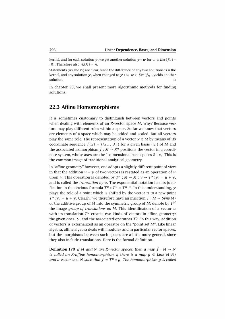
296 Linear Dependence, Bases, and Dimension
kernel, and for each solution y , we get another solution y+w forw ∈ Ker(fM)−{0}. Therefore also rk(M) = n.
Statements (iv) and (v) are clear, since the difference of any two solutions is n the
kernel, and any solution y , when changed to y+w,w ∈ Ker(fM), yields another
solution. �
In chapter 23, we shall present more algorithmic methods for finding
solutions.
22.3 Affine Homomorphisms
It is sometimes customary to distinguish between vectors and points
when dealing with elements of an R-vector space M . Why? Because vec-
tors may play different roles within a space. So far we know that vectors
are elements of a space which may be added and scaled. But all vectors
play the same role. The representation of a vector x ∈ M by means of its
coordinate sequence f(x) = (λ1, . . . λn) for a given basis (xi) of M and
the associated isomorphism f : M∼→ Rn positions the vector in a coordi-
nate system, whose axes are the 1-dimensional base spaces R ·xi. This is
the common image of traditional analytical geometry.
In “affine geometry” however, one adopts a slightly different point of view
in that the addition u+y of two vectors is restated as an operation of u
upon y . This operation is denoted by Tu : M → M : y , Tu(y) = u+ y ,
and is called the translation by u. The exponential notation has its justi-
fication in the obvious formula Tu ◦ Tv = Tu+v . In this understanding, y
plays the role of a point which is shifted by the vector u to a new point
Tu(y) = u+ y . Clearly, we therefore have an injection T : M → Sym(M)
of the additive group of M into the symmetric group of M ; denote by TM
the image group of translations on M . This identification of a vector u
with its translation Tu creates two kinds of vectors in affine geometry:
the given ones, y , and the associated operators Ty . In this way, addition
of vectors is externalized as an operator on the “point set M”. Like linear
algebra, affine algebra deals with modules and in particular vector spaces,
but the morphisms between such spaces are a little more general, since
they also include translations. Here is the formal definition.
Definition 170 If M and N are R-vector spaces, then a map f : M → Nis called an R-affine homomorphism, if there is a map g ∈ LinR(M,N)
and a vector u ∈ N such that f = Tu ◦ g. The homomorphism g is called
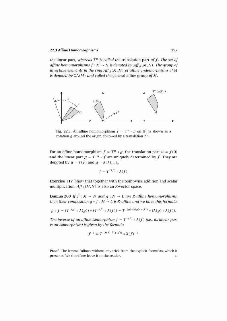
22.3 Affine Homomorphisms 297
the linear part, whereas Tu is called the translation part of f . The set of
affine homomorphisms f : M → N is denoted by Aff R(M,N). The group of
invertible elements in the ring Aff R(M,M) of affine endomorphisms of M
is denoted by GA(M) and called the general affine group of M .
Fig. 22.3. An affine homomorphism f = Tu ◦ g on R2 is shown as a
rotation g around the origin, followed by a translation T u.
For an affine homomorphism f = Tu ◦ g, the translation part u = f(0)and the linear part g = T−u ◦ f are uniquely determined by f . They are
denoted by u = τ(f) and g = λ(f), i.e.,
f = T τ(f) ◦ λ(f).
Exercise 117 Show that together with the point-wise addition and scalar
multiplication, Aff R(M,N) is also an R-vector space.
Lemma 200 If f : M → N and g : N → L are R-affine homomorphisms,
then their composition g ◦ f : M → L is R-affine and we have this formula:
g ◦ f = (T τ(g) ◦ λ(g)) ◦ (T τ(f) ◦ λ(f)) = T τ(g)+λ(g)(τ(f )) ◦ (λ(g) ◦ λ(f)).
The inverse of an affine isomorphism f = T τ(f) ◦ λ(f) (i.e., its linear part
is an isomorphism) is given by the formula
f−1 = T−λ(f)−1(τ(f )) ◦ λ(f)−1.
Proof The lemma follows without any trick from the explicit formulas, which it
presents. We therefore leave it to the reader. �

298 Linear Dependence, Bases, and Dimension
Fig. 22.4. Composition g ◦ f of affine homomorphisms g and f acting
on a vector u.
Exercise 118 Show that the group TM of translations is a normal sub-
group of GA(M). Show that GA(M)/TM∼→ GL(M).
It has turned out advantageous to represent linear maps by matrixes, so
let us see how this can be obtained for affine maps. Of course, the usual
representation does not work, because, in general, affine maps do leave
origin fixed. But there is a beautiful trick to interpret an affine map as if
it would. The trick consists in inventing a new origin and embedding the
given vector space in a larger space, where we have a linear map which on
the embedded space behaves like the given affine map. The new system is
related to what is known as the method of “homogeneous coordinates”.
We have the affine injection
ηM : M → M ⊕ R :m , (m,1)
of homogenization, i.e., ηM = T (0,1) ◦ i1, where i1 is the usual linear em-
bedding of M as first summand of M ⊕ R. Then, for a given affine homo-
morphism f : M → N, we consider the linear homomorphism
f : M ⊕ R → N ⊕ R : (m, r), (λ(f)(m),0)+ r(τ(f),1)
associated with an affine homomorphism f : M → N. Clearly, f sends
ηM(M) to ηN(N). More precisely, we have
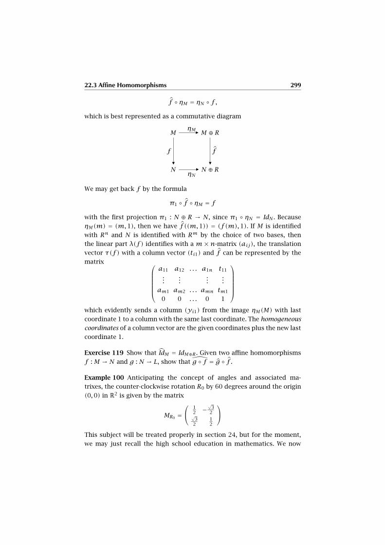
22.3 Affine Homomorphisms 299
f ◦ ηM = ηN ◦ f ,
which is best represented as a commutative diagram
MηM
ñ M ⊕ R
N
f
�
ηNñ N ⊕ R
f
�
We may get back f by the formula
π1 ◦ f ◦ ηM = f
with the first projection π1 : N ⊕ R → N, since π1 ◦ ηN = IdN . Because
ηM(m) = (m,1), then we have f ((m,1)) = (f (m),1). If M is identified
with Rn and N is identified with Rm by the choice of two bases, then
the linear part λ(f) identifies with a m × n-matrix (aij), the translation
vector τ(f) with a column vector (ti1) and f can be represented by the
matrix
a11 a12 . . . a1n t11
......
......
am1 am2 . . . amn tm1
0 0 . . . 0 1
which evidently sends a column (yi1) from the image ηM(M) with last
coordinate 1 to a column with the same last coordinate. The homogeneous
coordinates of a column vector are the given coordinates plus the new last
coordinate 1.
Exercise 119 Show that IdM = IdM⊕R. Given two affine homomorphisms
f : M → N and g : N → L, show that g ◦ f = g ◦ f .
Example 100 Anticipating the concept of angles and associated ma-
trixes, the counter-clockwise rotation R0 by 60 degrees around the origin
(0,0) in R2 is given by the matrix
MR0 =
12 −
√3
2√3
212
This subject will be treated properly in section 24, but for the moment,
we may just recall the high school education in mathematics. We now
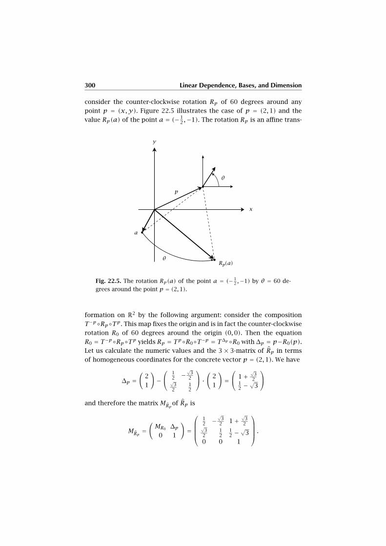
300 Linear Dependence, Bases, and Dimension
consider the counter-clockwise rotation Rp of 60 degrees around any
point p = (x,y). Figure 22.5 illustrates the case of p = (2,1) and the
value Rp(a) of the point a = (− 12 ,−1). The rotation Rp is an affine trans-
Fig. 22.5. The rotation Rp(a) of the point a = (− 12 ,−1) by θ = 60 de-
grees around the point p = (2,1).
formation on R2 by the following argument: consider the composition
T−p◦Rp◦Tp. This map fixes the origin and is in fact the counter-clockwise
rotation R0 of 60 degrees around the origin (0,0). Then the equation
R0 = T−p◦Rp◦Tp yields Rp = Tp◦R0◦T−p = T∆p◦R0 with ∆p = p−R0(p).
Let us calculate the numeric values and the 3 × 3-matrix of Rp in terms
of homogeneous coordinates for the concrete vector p = (2,1). We have
∆p =(
2
1
)−
12 −
√3
2√3
212
·
(2
1
)= 1+
√3
212 −√
3
and therefore the matrix MRpof Rp is
MRp =(MR0 ∆p
0 1
)=
12 −
√3
2 1+√
32√
32
12
12 −√
3
0 0 1
.

22.3 Affine Homomorphisms 301
The transformation corresponding to MRp is shown in figure 22.6. If ap-
plied to a vector a = (− 12 ,−1), rewritten in homogeneous coordinates
a = (−12 ,−1,1), we get the product
Rp(a)τ =
12 −
√3
2 1+√
32√
32
12
12 −√
3
0 0 1
·
−12
−1
1
=
34 +√
3
−5√
34
1
.
Fig. 22.6. The same transformation as in figure 22.5, but this time in
homogeneous coordinates, i.e., Rp(a), where a = (− 12 ,−1,1).

CHAPTER 23
Algorithms in Linear Algebra
In practice, one needs algorithmic methods to calculate matrixes which
arise from problems in linear algebra or vector spaces. In particular, it is
important to obtain solutions of linear equations, to calculate determi-
nants and inverse matrixes. This is a vast field of numerical mathematics
and of ongoing research, since fast and reliable algorithms for special ma-
trixes are of crucial importance for the entire computer-aided science, be
it physics, economics, chemistry or biology. There are also very important
applications of matrix calculations in special technological fields such as
signal processing (e.g., Fast Fourier Transform, see later in the second
volume of this book), which are particularly sensitive to fast methods be-
cause they pertain to real-time applications. We shall only discuss some
very elementary algorithms here in order to give a first idea of the sub-
ject. For object-oriented implementations of these and other algorithms,
we refer to [6].
23.1 Gauss Elimination
The Gauss algorithm is based on two simple observations about the so-
lutions of linear equations:
1. If we are given a linear equation y = f(x) for an R-linear map f : M →N, the solutions x are unchanged if we compose f with a g ∈ GL(N)
and thus obtain the new equation g(y) = g(f(x)) = (g ◦ f)(x).
304 Algorithms in Linear Algebra
2. If we have a well-known h ∈ GL(M), then we may rewrite the equation
as y = f(x) = (f ◦h−1)◦h(x), and hope that the new unknown h(x)
is easier to manage than the original one.
The first observation can be applied to matrixes as follows: We are given
a system of linear equations
yi =∑
j=0,...n
aij · xj
with m equations (i = 1, . . .m) and n unknowns (j = 1, . . . n). This can
be written as matrix equation
y = A · x
where A = (aij), x = (xj) and y = (yi). Then the solution set is left
unchanged if we multiply both sides by an invertible m ×m-matrix B,
obtaining the new matrix equation
y ′ = B ·y = (B ·A) · x = A′ · x.
The second observation suggests that we take an invertible n×n-matrix
C and rewrite
y = A · x = (A · C−1) · (C · x) = A′ · x′
with the new unknowns
x′ = C · x.
The method of Gauss elimination consists of a clever choice of a series
of transformations B and C which successively change the equation until
it has a particularly simple shape. Mostly, Gauss elimination is applied
in the case of a regular system of n equations with n unknowns, i.e.,
the coefficient matrix A is supposed to be invertible, such that we have
exactly one solution.
The idea of this procedure is to obtain an upper triangular coefficient
matrix A, i.e., aij = 0 for i > j. This means that the diagonal elements
aii ≠ 0, because their product is the non-zero determinant. Then we may
solve the equation system by backward substitution, which means that
we first calculate xn, then xn−1, etc. until we obtain the solution of x1. In
fact, a triangular matrix yields these n equations:
23.1 Gauss Elimination 305
yi =∑
j=i,i+1,...n
aijxj
which can be solved recursively, beginning with
xn = 1
annyn
and yielding
xi =yi −
∑j=i+1,...n aijxj
aii
from the calculation of xn, xn−1, . . . xi+1.
So we are left with the construction of an upper triangular coefficient
matrix. Again, this is a recursive construction, proceeding along the size
n. To begin with, one would like to have a11 ≠ 0. If this is not the case, we
look for a first index k > 1 such that a1k ≠ 0. This exists since otherwise,
the determinant of A would vanish. Now we rename the unknowns: x1
becomes xk, and xk becomes x1. This is achieved by replacing A with
A′ = A·P(1, k) and the column x with x′ = P(1, k)·x. The matrix P(1, k)
corresponds to the transposition (1k) in the symmetric group Sn and is
defined by P(1, k) = En − E(1,1)− E(k, k)+ E(k,1)+ E(1, k). Multiplying
A from the right by P(1, k) exchanges column 1 and k of A, whereas
multiplying x by P(1, k) from the left, exchanges x1 and xk, and this
does not change anything in the product y = A′ ·x′, since P(1, k)2 = En.
Therefore, up to renaming x1 to x′k, and xk to x′1, and leaving all other
unknowns xj = x′j , we have achieved that a11 ≠ 0. Next, we find an
invertible B such that A′ = B · A has zeros a′ij = 0 i > j. This is the
matrix:
B = En −∑
i=2,...n
ai1
a11· E(i,1).
It is invertible (the determinant is 1) and and the product A′ = B ·A has
zeros a′i1 = 0, for i > 1. Proceeding recursively, the situation is restricted
to the equations i = 2, . . . n involving only the unknowns x2, . . . xn. This
settles the problem.
Example 101 Consider the system of equations
2x1 + 3x2 + 4x3 = 8
4x1 + 2x2 − x3 = −3
2x1 − 3x2 + 3x3 = 17
This can be rewritten as
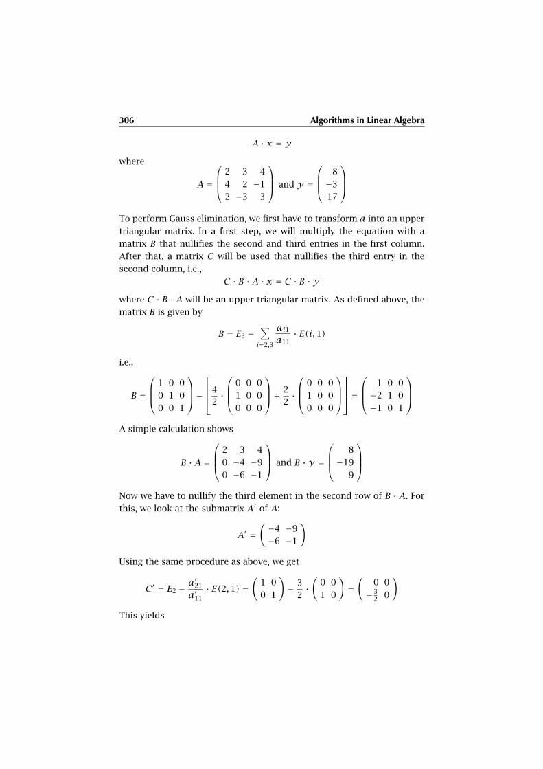
306 Algorithms in Linear Algebra
A · x = ywhere
A =
2 3 4
4 2 −1
2 −3 3
and y =
8
−3
17
To perform Gauss elimination, we first have to transform a into an upper
triangular matrix. In a first step, we will multiply the equation with a
matrix B that nullifies the second and third entries in the first column.
After that, a matrix C will be used that nullifies the third entry in the
second column, i.e.,
C · B ·A · x = C · B ·ywhere C · B · A will be an upper triangular matrix. As defined above, the
matrix B is given by
B = E3 −∑
i=2,3
ai1
a11· E(i,1)
i.e.,
B =
1 0 0
0 1 0
0 0 1
−
4
2·
0 0 0
1 0 0
0 0 0
+
2
2·
0 0 0
1 0 0
0 0 0
=
1 0 0
−2 1 0
−1 0 1
A simple calculation shows
B ·A =
2 3 4
0 −4 −9
0 −6 −1
and B ·y =
8
−19
9
Now we have to nullify the third element in the second row of B · A. For
this, we look at the submatrix A′ of A:
A′ =(−4 −9
−6 −1
)
Using the same procedure as above, we get
C′ = E2 − a′21
a′11· E(2,1) =
(1 0
0 1
)− 3
2·(
0 0
1 0
)=(
0 0
−32 0
)
This yields
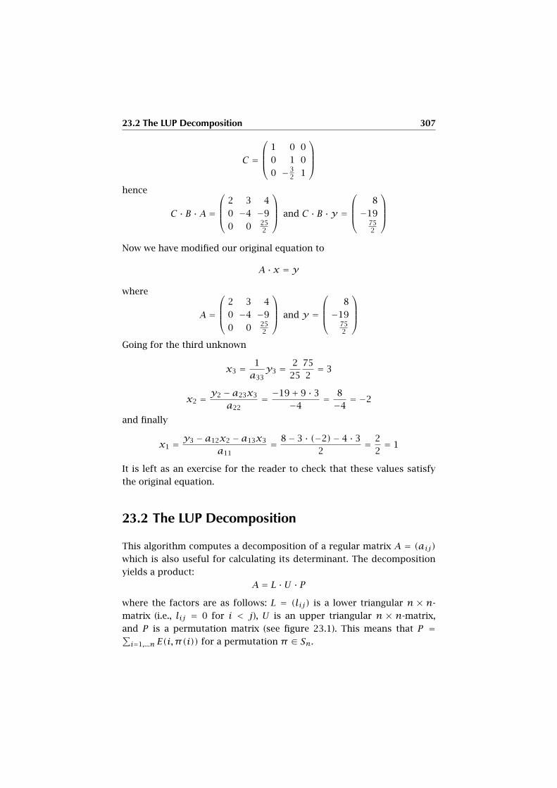
23.2 The LUP Decomposition 307
C =
1 0 0
0 1 0
0 −32 1
hence
C · B ·A =
2 3 4
0 −4 −9
0 0 252
and C · B ·y =
8
−19752
Now we have modified our original equation to
A · x = y
where
A =
2 3 4
0 −4 −9
0 0 252
and y =
8
−19752
Going for the third unknown
x3 = 1
a33y3 = 2
25
75
2= 3
x2 = y2 − a23x3
a22= −19+ 9 · 3
−4= 8
−4= −2
and finally
x1 = y3 − a12x2 − a13x3
a11= 8− 3 · (−2)− 4 · 3
2= 2
2= 1
It is left as an exercise for the reader to check that these values satisfy
the original equation.
23.2 The LUP Decomposition
This algorithm computes a decomposition of a regular matrix A = (aij)which is also useful for calculating its determinant. The decomposition
yields a product:
A = L ·U · Pwhere the factors are as follows: L = (lij) is a lower triangular n × n-
matrix (i.e., lij = 0 for i < j), U is an upper triangular n × n-matrix,
and P is a permutation matrix (see figure 23.1). This means that P =∑i=1,...n E(i,π(i)) for a permutation π ∈ Sn.
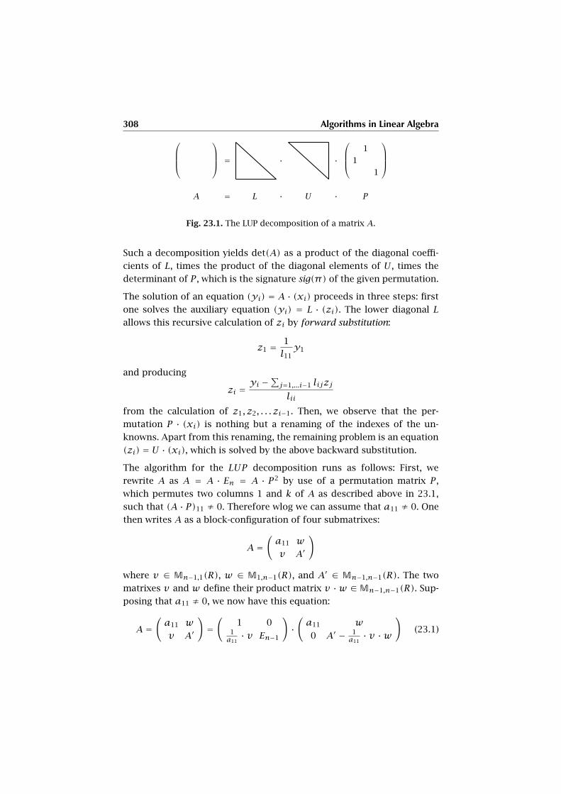
308 Algorithms in Linear Algebra
= · ·
1
1
1
A = L · U · P
Fig. 23.1. The LUP decomposition of a matrix A.
Such a decomposition yields det(A) as a product of the diagonal coeffi-
cients of L, times the product of the diagonal elements of U , times the
determinant of P , which is the signature sig(π) of the given permutation.
The solution of an equation (yi) = A · (xi) proceeds in three steps: first
one solves the auxiliary equation (yi) = L · (zi). The lower diagonal L
allows this recursive calculation of zi by forward substitution:
z1 = 1
l11y1
and producing
zi =yi −
∑j=1,...i−1 lijzj
lii
from the calculation of z1, z2, . . . zi−1. Then, we observe that the per-
mutation P · (xi) is nothing but a renaming of the indexes of the un-
knowns. Apart from this renaming, the remaining problem is an equation
(zi) = U · (xi), which is solved by the above backward substitution.
The algorithm for the LUP decomposition runs as follows: First, we
rewrite A as A = A · En = A · P2 by use of a permutation matrix P ,
which permutes two columns 1 and k of A as described above in 23.1,
such that (A · P)11 ≠ 0. Therefore wlog we can assume that a11 ≠ 0. One
then writes A as a block-configuration of four submatrixes:
A =(a11 w
v A′
)
where v ∈ Mn−1,1(R), w ∈ M1,n−1(R), and A′ ∈ Mn−1,n−1(R). The two
matrixes v and w define their product matrix v ·w ∈Mn−1,n−1(R). Sup-
posing that a11 ≠ 0, we now have this equation:
A =(a11 w
v A′
)=(
1 01a11· v En−1
)·(a11 w
0 A′ − 1a11· v ·w
)(23.1)
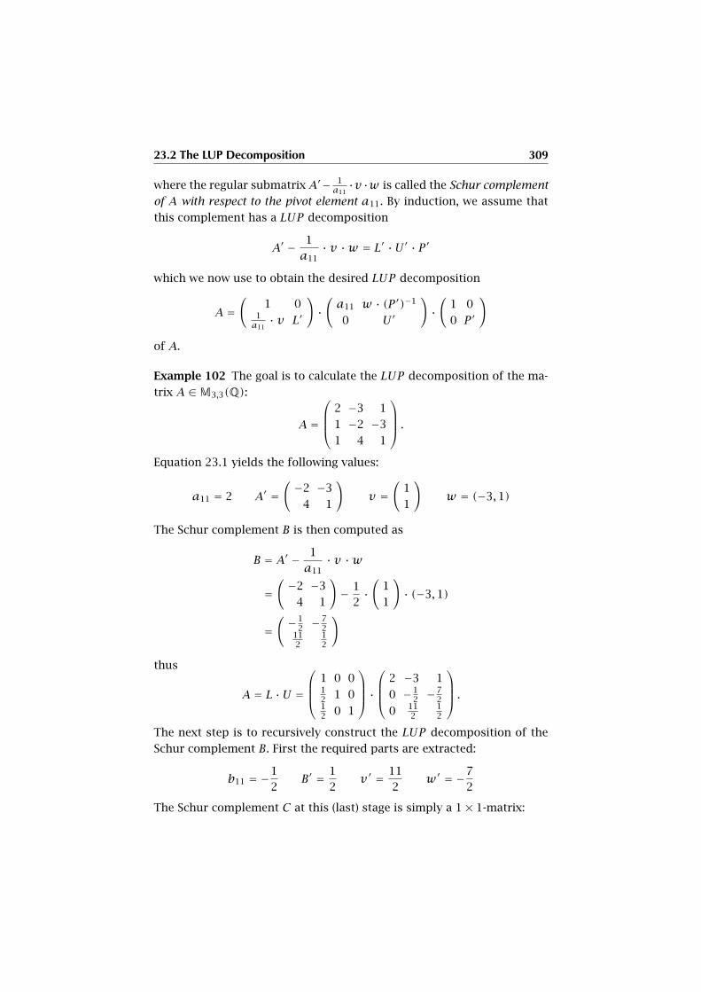
23.2 The LUP Decomposition 309
where the regular submatrix A′− 1a11·v ·w is called the Schur complement
of A with respect to the pivot element a11. By induction, we assume that
this complement has a LUP decomposition
A′ − 1
a11· v ·w = L′ ·U ′ · P ′
which we now use to obtain the desired LUP decomposition
A =(
1 01a11· v L′
)·(a11 w · (P ′)−1
0 U ′
)·(
1 0
0 P ′
)
of A.
Example 102 The goal is to calculate the LUP decomposition of the ma-
trix A ∈M3,3(Q):
A =
2 −3 1
1 −2 −3
1 4 1
.
Equation 23.1 yields the following values:
a11 = 2 A′ =( −2 −3
4 1
)v =
(1
1
)w = (−3,1)
The Schur complement B is then computed as
B = A′ − 1
a11· v ·w
=( −2 −3
4 1
)− 1
2·(
1
1
)· (−3,1)
=( −1
2 −72
112
12
)
thus
A = L ·U =
1 0 012 1 012 0 1
·
2 −3 1
0 −12 −7
2
0 112
12
.
The next step is to recursively construct the LUP decomposition of the
Schur complement B. First the required parts are extracted:
b11 = −1
2B′ = 1
2v′ = 11
2w′ = −7
2
The Schur complement C at this (last) stage is simply a 1× 1-matrix:

310 Algorithms in Linear Algebra
C = B′ − 1
b11· v′ ·w′
= 1
2+ 2 · 11
2· −7
2
= −38
therefore
B = L′ ·U ′ =(
1 0
−11 1
)·(−1
2 −72
0 −38
).
Finally, the LUP decomposition is built up using the components just
determined. Luckily, during the entire procedure there has never been a
need for an exchange of columns; all permutation matrixes are therefore
unit matrixes and can be omitted:
A =
1 0 012 1 012 −11 1
·
2 −3 1
0 −12 −7
2
0 0 −38
It is now easy to calculate the determinant of A:
det(A) = det(L) · det(U) = 1 · 1 · 1 · 2 · −1
2· −38 = 38
Of course, in this case we could have applied the formula for determi-
nants of 3×3-matrixes, but in larger sized matrixes, the LUP decomposi-
tion provides a much more efficient procedure than using the definition
of determinants directly.

CHAPTER 24
Linear Geometry
The previous mathematical development has covered a considerable
number of familiar objects and relations, such as sets, numbers, graphs,
grammars, or rectangular tables, which are abstractly recast in the ma-
trix calculus. The axiomatic treatment of modules and, more specifically,
vector spaces, has also allowed us to rebuild what is commonly known
as coordinate systems. However, one very important aspect of everyday’s
occupation with geometric objects has not been even alluded to: distance
between objects, angles between straight lines, lengths of straight lines
connecting two points in space. Even more radically, the concept of a
neighborhood has not been thematized, although it is a central concept
in the comparison of positions of objects in a sensorial space, such as
the visual, tactile, gestural, or auditive space-time. The following chapter
is devoted to the very first steps towards the concept of a mathematical
model of geometric reality (the Greek etymology of “geometry” being “to
measure the earth”). In this spirit, we shall exclusively deal with real vector
spaces in the last two chapters of this part, i.e., the coefficient set is R. We
shall also assume that the vector spaces are always of finite dimension—
unless the contrary is stated.
24.1 Euclidean Vector Spaces
We begin with some preliminary definitions. For a real vector space V ,
the vector space of linear homomorphisms LinR(V ,R) is called the dual
space of V and denoted by V∗. If V is finite-dimensional of dimension

312 Linear Geometry
dim(V) = n, then we know that V∗ ∼→ M1,n(R)∼→ Rn
∼→ V . A linear map
l ∈ V∗ is called an R-linear form on V .
In order to generate the basic metric structures, one first needs bilinear
forms:
Definition 171 Given a real vector space V , a map b : V ×V → R is called
R-bilinear iff for each v ∈ V , both maps b(v, ?) : V → R : x , b(v,x) and
b(?, v) : V → R : x , b(x,v) are R-linear forms. A bilinear form is called
symmetric iff b(x,y) = b(y,x) for all (x,y) ∈ V ×V . It is called positive
definite iff b(x,x) > 0 for all x ≠ 0.
Given a symmetric, positive definite bilinear form b, the pair (V , b) is
called a Euclidean vector space.
An isometry f : (V , b) → (W, c) between Euclidean spaces is a linear map
f ∈ LinR(V ,W) such that for all (x,y) ∈ V ×V , we have c(f(x), f (y)) =b(x,y). The set of isometries f : (V , b) → (W, c) is denoted by Ob,c(V ,W)
or O(V ,W) if the bilinear forms are clear. If (V , b) = (W, c), one writes
O(V) instead.
For a vector x in a Euclidean vector space (V , b), the norm of x is the
non-negative real number ‖x‖ = √b(x,x).
Lemma 201 For a Euclidean space (V , b), the norm has this property for
any vectors x,y ∈ V :
‖x +y‖2 = ‖x‖2 + 2 · b(x,y)+ ‖y‖2,
On the other hand, the form b is determined by the associated norm with
the formula
b(x,y) = 1
2(‖x +y‖2 − ‖x‖2 − ‖y‖2).
Proof We have
‖x +y‖2 = b(x +y,x +y)= b(x,x)+ b(x,y)+ b(y,x)+ b(y,y)= ‖x‖2 + 2 · b(x,y)+ ‖y‖2.
�
Lemma 202 For a finite-dimensional Euclidean space (V , b), the map∗b : V → V∗ : v , b(v, ?) is a linear isomorphism and is equal to the
map b∗ : V → V∗ : v , b(?, v).
24.1 Euclidean Vector Spaces 313
Proof The map v , b(v, ?), where b(v, ?) : V → R : w , b(v,w), maps into
V∗, where dim(V∗) = dim(V) according to the remark at the beginning of this
section. So it is sufficient to show that ∗b is a linear injection. If b(v, ?) = 0, then
also b(v,v) = 0, but then, v = 0, since b is positive definite. Further b(v1 +v2,w) = b(v1,w) + b(v2,w), and b(λ · v,w) = λ · b(v,w), so ∗b is linear. By
symmetry of b, we also have b∗ = ∗b. �
Exercise 120 Let (V , b) be a Euclidean space and f : V → V is a lin-
ear endomorphism. Prove that for any x ∈ V , the map y , b(x, f (y))
is a linear form. By lemma 202, there is a vector τf(x) ∈ V such that
b(x, f (y)) = b(τf(x),y) for all y . Show that τf is a linear map. It is
called the adjoint of f .
Proposition 203 An isometry f ∈ O(V ,W) is always injective, and it is an
isomorphism, whose inverse is also an isometry, if V and W have the same
finite dimension n. The composition g ◦f of two isometries f : V → W and
g : W → X is an isometry, and O(V) is a subgroup of GL(V), called the
orthogonal group of V .
Proof For an isometry f : (V , b) → (W, c) and v ∈ V , ‖f(v)‖ = ‖v‖ in the
respective norms, i.e., f conserves norms. But then, if v ≠ 0, f(v) ≠ 0, so f
is injective. If both spaces have the same finite dimension, f must also be sur-
jective, and the inverses of such isometries also conserve norms, and norms
define the bilinear forms. So they are also isometries. Further, the composition
of isometries is an isometry, since conservation of norms is a transitive relation.
Hence O(V) is a subgroup of GL(V). �
Exercise 121 For V = Rn, n > 0, we have the standard bilinear form
(?, ?) : Rn ×Rn → R, or scalar product with
((x1, . . . xn), (y1, . . . yn)) = (x1, . . . xn) · (y1, . . . yn)τ =
∑
i=1,...n
xiyi,
the product of a row and a column matrix, where we omit the parentheses
surrounding the resulting number. Show that the standard bilinear form
is symmetric and positive definite.
The bilinear form of any non-zero Euclidean space can be calculated by
means of matrix products as follows: Let (ei)i=1...n be a basis of V , and
define the associated matrix of the bilinear form by B = (Bij) ∈ Mn,n(R)
with Bij = b(ei, ej). Then the bilinearity of b implies the following for-
mula for the representations x = ∑i ξiei and y = ∑i ηiei of the vectors
x and y by their n-tuples in Rn:
314 Linear Geometry
b(x,y) = (ξi) · (Bij) · (ηj)τ
One recognizes that the scalar product defined above is the special case
of a bilinear form where (Bij) = (δij) = En. The question, whether one
may find a basis for every Euclidean space such that its associated ma-
trix becomes this simple, can be answered by “yes!”, but we need some
auxiliary theory which will also justify the hitherto mysterious wording
“orthogonal group”.
Definition 172 In a Euclidean space (V , b), a vector x is said to be orthog-
onal to a vector y iff b(x,y) = 0, in signs: x⊥y . Since b is symmetric,
orthogonality is a symmetric relation. A sequence (x1, . . . xk) of vectors in
V is called orthogonal iff xi⊥xj for all i ≠ j. It is called orthonormal iff it
is orthogonal and we have ‖xi‖ = 1 for all i.
Two subspaces U,W ⊂ V are called orthogonal to each other, in signs
U⊥W iff u⊥w for all u ∈ U andw ∈ W . The subspace of all vectors which
are orthogonal to a subspace U is the largest subspace orthogonal to U
and is denoted by U⊥.
Proposition 204 (Gram-Schmidt Orthonormalization) If (x1 . . . xk) with
k > 0 is a sequence of linearly independent vectors in a Euclidean space
(V , b), then there is an orthonormal sequence (e1 . . . ek) of linearly in-
dependent vectors such that for every index i = 1, . . . k, (x1 . . . xi) and
(e1 . . . ei) generate the same subspace. In particular, if (x1 . . . xn) is a ba-
sis of V , then there is a orthonormal basis (e1, . . . en) such that (x1 . . . xi)
and (e1 . . . ei) generate the same subspaces for all i = 1, . . . n.
Proof The construction is by induction on the length k of the sequence. For
k = 1, e1 = 1‖x1‖x1 does the job. Suppose that all x1, x2, . . . xi are represented by
an orthonormal sequence e1, e2, . . . ei in the required way. Setting ei+1 = xi+1 +∑j=1,...i λjej , if we find a solution, then clearly the space generated by x1, . . . xi+1
coincides with the space generated by e1, . . . ei+1. But the condition that ei+1⊥ej ,for all j = 1, . . . i, means that b(ej , xi+1) + λj · ‖ej‖2 = 0, which yields λj =−b(ej , xi+1), since ‖ej‖ = 1. Now, the resulting ei+1 is orthogonal to all previous
ej and cannot vanish, because of the dimension i+ 1 of the subspace generated
by e1, . . . ei+1. So, to obtain the correct norm 1 of ei+1, replace it by 1‖ei+1‖ei+1,
and everything is perfect. �
Observe that the proof of proposition 204 is constructive, i.e., algorith-
mic, and should be kept in mind together with the result.
24.1 Euclidean Vector Spaces 315
Example 103 Let x1 = (2,2,0), x2 = (1,0,2) and x3 = (0,2,1) be a ba-
sis of R3. We compute an orthonormal basis {e1, e2, e3} using the Gram-
Schmidt procedure. For the linear form b we use the ordinary scalar prod-
uct.
The computation of e1 is simple. It consists in normalizing x1:
e1 = 1
‖x1‖x1
= 1√22 + 22 + 02
(2,2,0)
= 1
2√
2(2,2,0)
=(√
2
2,
√2
2,0
)
For the second vector e2 we first compute an intermediate value e′2 usingthe formula from the proof of proposition 204:
e′2 = x2 − (e1, x2) · e1
= (1,0,2)−((√
2
2,
√2
2,0
), (1,0,2)
)·(√
2
2,
√2
2,0
)
= (1,0,2)−√
2
2·(√
2
2,
√2
2,0
)
=(
1−√
2
2·√
2
2,−√
2
2·√
2
2,2
)
=(
1
2,−1
2,2)
and then normalize to get e2:
e2 = 1
‖e′2‖e′2
= 1√1/22 + 1/22 + 22
(1
2,−1
2,2)=√
2
3
(1
2,−1
2,2)
=(√
2
6,−√
2
6,2√
2
3
)
The formula for the last vector becomes more complex:
316 Linear Geometry
e′3 = x3 − (e1, x3) · e1 − (e2, x3) · e2
= x3 −((√
2
2,
√2
2,0
), (0,2,1)
)· e1 −
((√2
6,−√
2
6,2√
2
3
), (0,2,1)
)· e2
= x3 −√
2 ·(√
2
2,
√2
2,0
)−√
2
3·(√
2
6,−√
2
6,2√
2
3
)
= (0,2,1)− (1,1,0)−(
1
9,−1
9,4
9
)
=(−10
9,10
9,5
9
)
Normalizing e′3 finally yields e3:
e3 = 1
‖e′3‖e′3
= 1√(−−10
9 )2 + (10
9 )2 + (5
9)2e′3
= 3
5·(−10
9,10
9,5
9
)
=(−2
3,2
3,1
3
)
Summarizing, the orthonormal basis is:
e1 =(√
2
2,
√2
2,0
), e2 =
(√2
6,−√
2
6,2√
2
3
), e3 =
(−2
3,2
3,1
3
)
Figure 24.1 shows both bases. It is left to the reader to check that the eiare indeed pairwise orthogonal.
Exercise 122 Show that, for an endomorphism f : V → V on a Euclidean
space, if A is the matrix of f with respect to an orthonormal basis, the
adjoint endomorphism τf has the transpose Aτ as its matrix with respect
to this basis.
Corollary 205 For an n-dimensional Euclidean space (V , b), if (ei) is an
orthonormal basis (which exists according to Gram-Schmidt), then the
group O(V) identifies with the subgroup On(R) ⊂ GLn(R) consisting
of all matrixes A with Aτ · A = En. In particular, det(f ) = ±1 for
f ∈ O(V). The orthogonal group is the disjoint union of the normal sub-
group SO(V) ⊂ O(V) of the isometries f with det(f ) = 1, called rotations,
and the coset O−(V) of the isometries f with det(f ) = −1. SO(V) is called
the special orthogonal group of V .
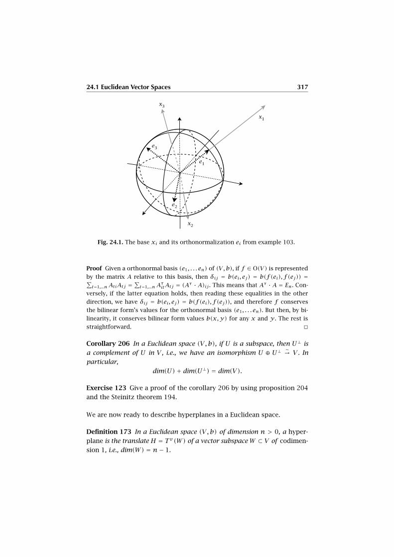
24.1 Euclidean Vector Spaces 317
Fig. 24.1. The base xi and its orthonormalization ei from example 103.
Proof Given a orthonormal basis (e1, . . . en) of (V , b), if f ∈ O(V) is represented
by the matrix A relative to this basis, then δij = b(ei, ej) = b(f(ei), f (ej)) =∑t=1,...nAtiAtj =
∑t=1,...nA
τitAtj = (Aτ ·A)ij . This means that Aτ ·A = En. Con-
versely, if the latter equation holds, then reading these equalities in the other
direction, we have δij = b(ei, ej) = b(f(ei), f (ej)), and therefore f conserves
the bilinear form’s values for the orthonormal basis (e1, . . . en). But then, by bi-
linearity, it conserves bilinear form values b(x,y) for any x and y . The rest is
straightforward. �
Corollary 206 In a Euclidean space (V , b), if U is a subspace, then U⊥ is
a complement of U in V , i.e., we have an isomorphism U ⊕ U⊥ ∼→ V . In
particular,
dim(U)+ dim(U⊥) = dim(V).
Exercise 123 Give a proof of the corollary 206 by using proposition 204
and the Steinitz theorem 194.
We are now ready to describe hyperplanes in a Euclidean space.
Definition 173 In a Euclidean space (V , b) of dimension n > 0, a hyper-
plane is the translate H = Tv(W) of a vector subspaceW ⊂ V of codimen-
sion 1, i.e., dim(W) = n− 1.
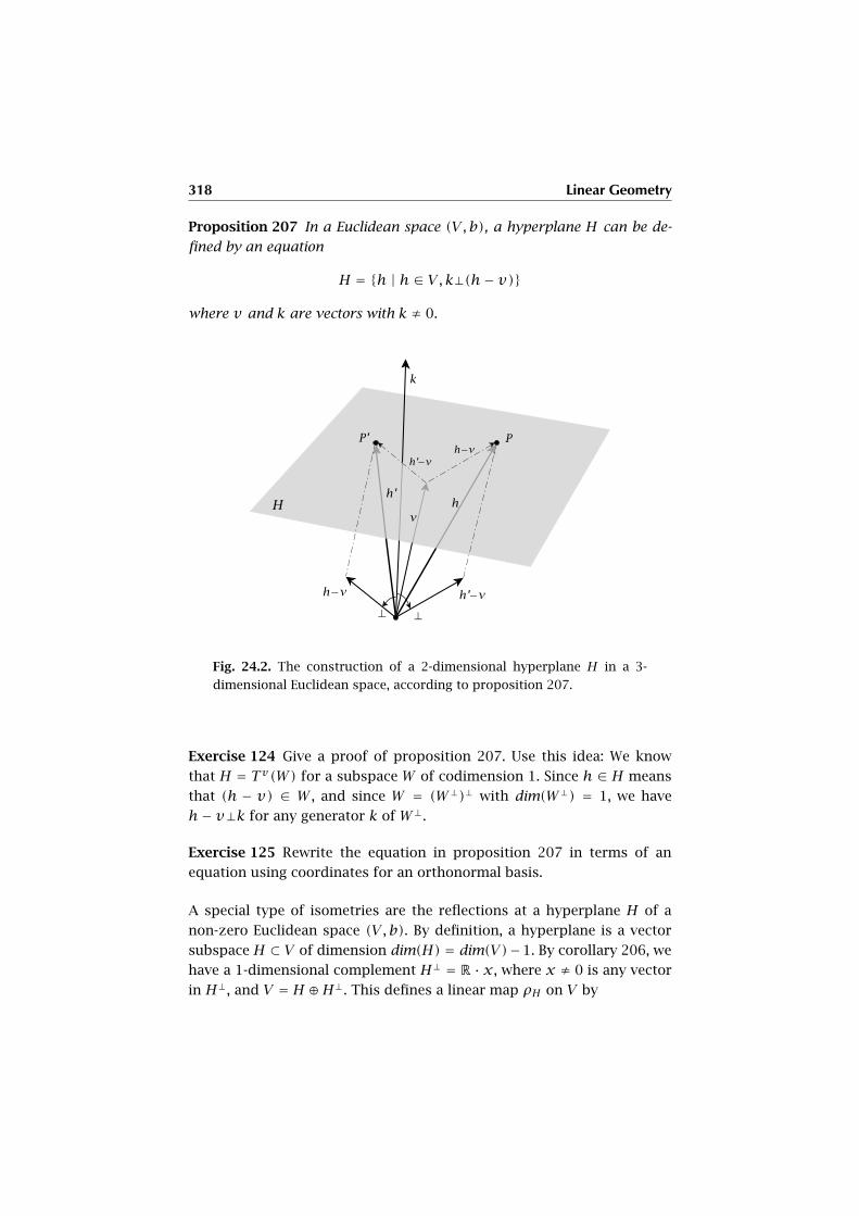
318 Linear Geometry
Proposition 207 In a Euclidean space (V , b), a hyperplane H can be de-
fined by an equation
H = {h | h ∈ V, k⊥(h− v)}
where v and k are vectors with k ≠ 0.
Fig. 24.2. The construction of a 2-dimensional hyperplane H in a 3-
dimensional Euclidean space, according to proposition 207.
Exercise 124 Give a proof of proposition 207. Use this idea: We know
that H = Tv(W) for a subspace W of codimension 1. Since h ∈ H means
that (h − v) ∈ W , and since W = (W⊥)⊥ with dim(W⊥) = 1, we have
h− v⊥k for any generator k of W⊥.
Exercise 125 Rewrite the equation in proposition 207 in terms of an
equation using coordinates for an orthonormal basis.
A special type of isometries are the reflections at a hyperplane H of a
non-zero Euclidean space (V , b). By definition, a hyperplane is a vector
subspace H ⊂ V of dimension dim(H) = dim(V)−1. By corollary 206, we
have a 1-dimensional complement H⊥ = R · x, where x ≠ 0 is any vector
in H⊥, and V = H ⊕H⊥. This defines a linear map ρH on V by
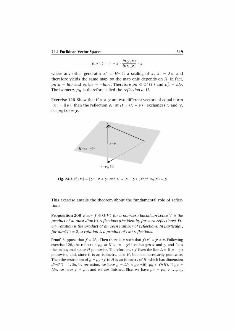
24.1 Euclidean Vector Spaces 319
ρH(y) = y − 2 · b(y,x)b(x,x)
· x
where any other generator x′ ∈ H⊥ is a scaling of x, x′ = λx, and
therefore yields the same map, so the map only depends on H. In fact,
ρH|H = IdH and ρH|H⊥ = −IdH⊥ . Therefore ρH ∈ O−(V) and ρ2H = IdV .
The isometry ρH is therefore called the reflection at H.
Exercise 126 Show that if x ≠ y are two different vectors of equal norm
‖x‖ = ‖y‖, then the reflection ρH at H = (x − y)⊥ exchanges x and y ,
i.e., ρH(x) = y .
Fig. 24.3. If ‖x‖ = ‖y‖, x ≠ y , and H = (x −y)⊥, then ρH(x) = y .
This exercise entails the theorem about the fundamental role of reflec-
tions:
Proposition 208 Every f ∈ O(V) for a non-zero Euclidean space V is the
product of at most dim(V) reflections (the identity for zero reflections). Ev-
ery rotation is the product of an even number of reflections. In particular,
for dim(V) = 2, a rotation is a product of two reflections.
Proof Suppose that f ≠ IdV . Then there is x such that f(x) = y ≠ x. Following
exercise 126, the reflection ρH at H = (x − y)⊥ exchanges x and y and fixes
the orthogonal space H pointwise. Therefore ρH ◦ f fixes the line ∆ = R(x − y)pointwise, and, since it is an isometry, also H, but not necessarily pointwise.
Then the restriction of g = ρH ◦f to H is an isometry of H, which has dimension
dim(V) − 1. So, by recursion, we have g = Id∆ × gH with gH ∈ O(H). If gH =IdH , we have f = ρH , and we are finished. Else, we have gH = ρH1 × . . . ρHk ,
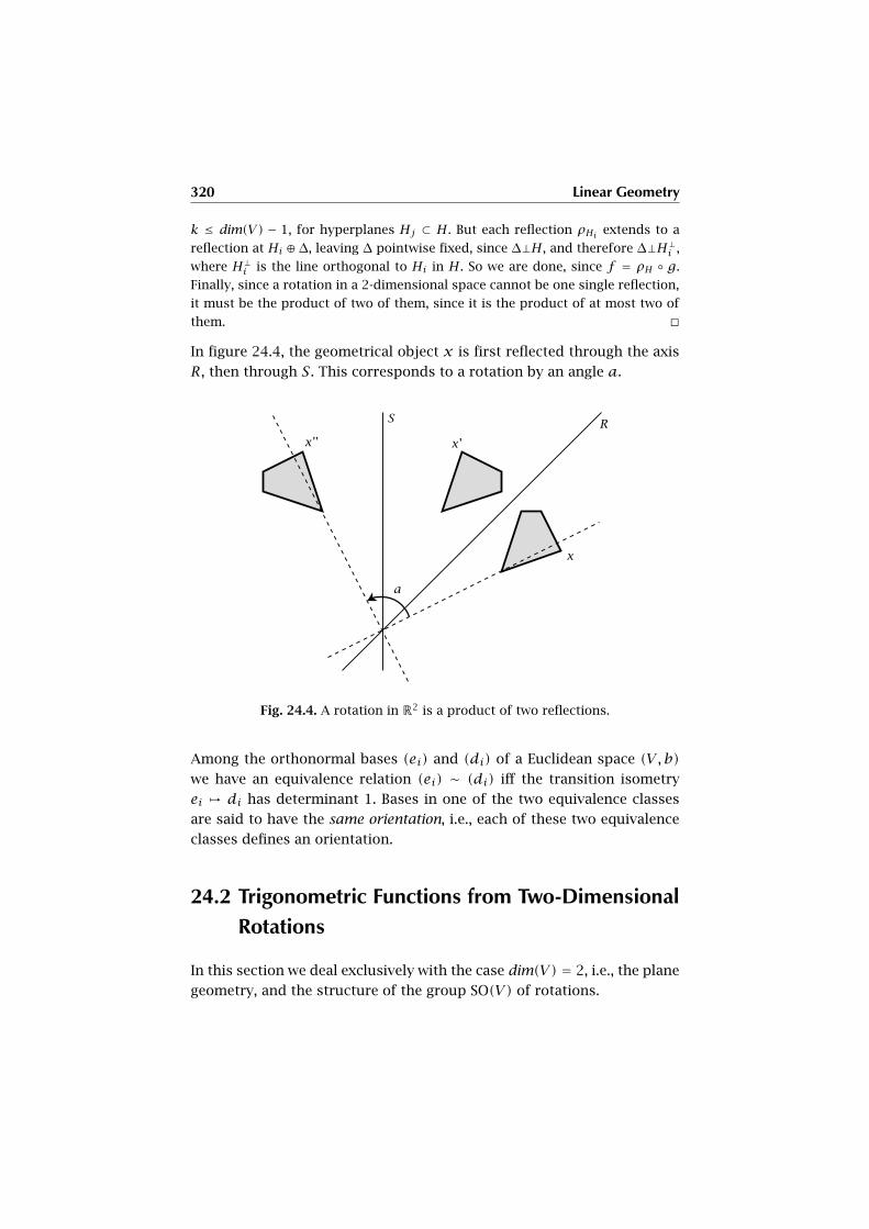
320 Linear Geometry
k ≤ dim(V) − 1, for hyperplanes Hj ⊂ H. But each reflection ρHi extends to a
reflection at Hi ⊕∆, leaving ∆ pointwise fixed, since ∆⊥H, and therefore ∆⊥H⊥i ,
where H⊥i is the line orthogonal to Hi in H. So we are done, since f = ρH ◦ g.
Finally, since a rotation in a 2-dimensional space cannot be one single reflection,
it must be the product of two of them, since it is the product of at most two of
them. �
In figure 24.4, the geometrical object x is first reflected through the axis
R, then through S. This corresponds to a rotation by an angle a.
Fig. 24.4. A rotation in R2 is a product of two reflections.
Among the orthonormal bases (ei) and (di) of a Euclidean space (V , b)
we have an equivalence relation (ei) ∼ (di) iff the transition isometry
ei , di has determinant 1. Bases in one of the two equivalence classes
are said to have the same orientation, i.e., each of these two equivalence
classes defines an orientation.
24.2 Trigonometric Functions from Two-Dimensional
Rotations
In this section we deal exclusively with the case dim(V) = 2, i.e., the plane
geometry, and the structure of the group SO(V) of rotations.

24.2 Trigonometric Functions from Two-Dimensional Rotations 321
Proposition 209 Given an orthonormal basis (ei) of V , let Mf ∈ M2,2(R)
be the associated matrix of an isometry f ∈ GL(V). Then
(i) we have f ∈ SO(V) (a rotation) iff Mf =(a −bb a
)and a2 + b2 = 1,
(ii) we have f ∈ O−(V) (a reflection) iffMf =(a b
b −a
)and a2+b2 = 1.
(iii) The group SO(V) is abelian and the product matrix for two rotations
f and g is
Mg ·Mf =(u −vv u
)·(a −bb a
)=(au− bv −(av + bu)av + bu au− bv
).
(iv) The number a is independent of the chosen orthonormal basis, and
so is |b|. If another orthonormal basis (e′i) with the same orientation
is chosen, then b does not change.
(v) For any two vectors x,y ∈ S(V) = {z | z ∈ V,‖z‖ = 1}, there is
exactly one f ∈ SO(V) such that f(x) = y .
Proof Clearly, concerning points (i) and (ii), according to corollary 205 the ma-
trixes in the described form define isometries f which are rotations or reflec-
tions, respectively. Conversely, if
(a
b
)is the first column of Mf , then we must
have a2 + b2 = 1, since the norm must be 1. On the other hand, the second col-
umn must be orthogonal to the first, and
( −ba
)is orthogonal to the first and
has norm 1. So
( −ba
)must be ±f(e2). But the determinant must be 1 if f is a
rotation, so the second column must be
( −ba
). Since the determinant must be
−1, if f is a reflection, the second column must be the negative of the first, so (i)
and (ii) are settled.
For point (iii), knowing that rotation matrixes have the shape described in (i), the
formula in (iii) shows that the product of rotations is commutative.
For (iv), we shall see in proposition 215 that the characteristic polynomial χMf (X)
of f is independent of its matrixMf (that result does not presuppose the present
one). But the coefficient of X in χf (X) is −2a with the notation described in (i)
and (ii). So a is uniquely determined, and therefore also |b|. If one changes the
base by a rotation, then the new matrix of f is the conjugate of the old matrix
by a rotation matrix. A straight calculation shows that b is also invariant.
Statement (v) follows from the fact that the orthogonal spaces x⊥ and y⊥ are
1-dimensional. So there are two possibilities to map a unit vector in x⊥ to a
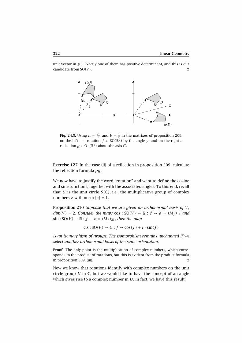
322 Linear Geometry
unit vector in y⊥. Exactly one of them has positive determinant, and this is our
candidate from SO(V). �
Fig. 24.5. Using a =√
32 and b = 1
2 in the matrixes of proposition 209,
on the left is a rotation f ∈ SO(R2) by the angle γ, and on the right a
reflection g ∈ O−(R2) about the axis G.
Exercise 127 In the case (ii) of a reflection in proposition 209, calculate
the reflection formula ρH .
We now have to justify the word “rotation” and want to define the cosine
and sine functions, together with the associated angles. To this end, recall
that U is the unit circle S(C), i.e., the multiplicative group of complex
numbers z with norm |z| = 1.
Proposition 210 Suppose that we are given an orthonormal basis of V ,
dim(V) = 2. Consider the maps cos : SO(V) → R : f , a = (Mf )11 and
sin : SO(V)→ R : f , b = (Mf )21, then the map
cis : SO(V)→ U : f , cos(f )+ i · sin(f )
is an isomorphism of groups. The isomorphism remains unchanged if we
select another orthonormal basis of the same orientation.
Proof The only point is the multiplication of complex numbers, which corre-
sponds to the product of rotations, but this is evident from the product formula
in proposition 209, (iii). �
Now we know that rotations identify with complex numbers on the unit
circle group U in C, but we would like to have the concept of an angle
which gives rise to a complex number in U . In fact, we have this result:
24.3 Gram’s Determinant and the Schwarz Inequality 323
Proposition 211 There is a surjective group homomorphism A : R →U whose kernel is Ker(A) = 2πZ, where π is the positive number
3.1415926 . . . which will in the chapter on limits and topology of the sec-
ond volume of this book. So with f ∈ SO(V) a coset of numbers θ ∈ R is
associated such that cos(f ) + i sin(f ) = A(θ). We also write cos(θ) and
sin(θ) instead of cos(f ) and sin(f ) respectively for the rotation associated
with θ. Any such θ is called angle of f . The matrix of f is:
Mf =(
cos(θ) − sin(θ)
sin(θ) cos(θ)
).
So the rotation angle θ is determined up to multiples of 2π . The product
formula in statement (iii) of proposition 209 translates into the classical
goniometric formulas for cos(θ ± η) and sin(θ ± η):
cos(θ ± η) = cos(θ) cos(η)∓ sin(θ) sin(η),
sin(θ ± η) = sin(θ) cos(η)± cos(θ) sin(η).
Proof The only point to be proved here are the formulas for cos(θ ± η) and
sin(θ ± η). But both relate to the cos and sin functions of sums/differences of
angles, and this means that one looks for the product of the rotations (or the
product of one with the inverse of the other) associated with these angles, i.e.,
cos(f ◦ g±1) and sin(f ◦ g±1). Then we know the formulas from the product
formula in proposition 209, (iii). �
24.3 Gram’s Determinant and the Schwarz Inequality
Given an n-dimensional Euclidean space (V , b) and an orthonormal basis
(ei), we may consider the determinant of the linear map associated with
a sequence x• = (xi) of length n by f : ei , xi. On the other hand, we
also have the Gram determinant Gram(xi) of (xi) defined by
Gram(xi) = det
b(x1, x1) b(x1, x2) . . . b(x1, xn)
b(x2, x1) b(x2, x2) . . . b(x2, xn)...
......
b(xn, x1) b(xn, x2) . . . b(xn, xn)
But the Gram matrix (b(xi, xj)) clearly equalsMτf ·Mf . Therefore we have
the Gram equation
324 Linear Geometry
Gram(xi) = det(f )2
For n = 2 we immediately deduce the Schwarz inequality:
Proposition 212 (Schwarz Inequality) If x and y are two vectors in a
Euclidean space (V , b), then
|b(x,y)| ≤ ‖x‖‖y‖,
equality holding iff x and y are linearly dependent.
Proof
0 ≤ det(f )2= Gram(x,y)
= det
(b(x,x) b(x,y)
b(y,x) b(y,y)
)
= b(x,x) · b(y,y)− b(x,y)2
Therefore, b(x,y)2 ≤ b(x,x)·b(y,y), which, due to the definition of the norm,
implies the desired result. �
This result may be reinterpreted in terms of the cosine function. If x,y ≠
0, choose a 2-dimensional subspace W of V containing x and y , and
carrying the induced bilinear form b|W×W . Then we have∣∣∣ b(x,y)‖x‖‖y‖
∣∣∣ ≤ 1,
and defining c(x,y) = b(x,y)‖x‖‖y‖ , we have b(x,y) = c(x,y) · ‖x‖ · ‖y‖
with |c(x,y)| ≤ 1. If f ∈ SO(W) is the unique rotation with f(x/‖x‖) =y/‖y‖, then c(x,y) = cos(f ) = cos(θ(x,y)), which means that the
angle is determined up to integer multiples of 2π by the unit vectors
x/‖x‖ and y/‖y‖ or equivalently the half lines R+x and R+y through
x and y . This gives us the famous cosine formula for the bilinear form,
where one has chosen an orthogonal basis on a plane containing x and
y :
b(x,y) = cos(θ(x,y)) · ‖x‖ · ‖y‖.
We also obtain the following intuitive fact: the triangle inequality for
norms.
Corollary 213 (Triangle Inequality) If x and y are two vectors in a Eu-
clidean space (V , b), then
‖x +y‖ ≤ ‖x‖ + ‖y‖.
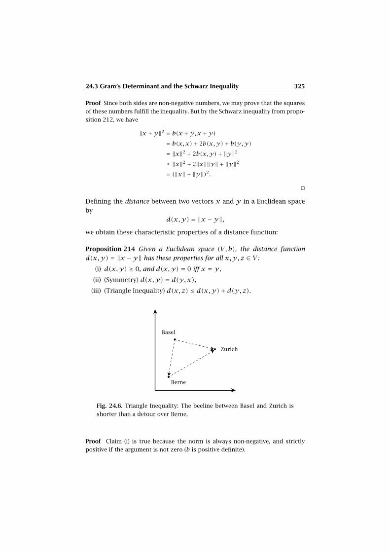
24.3 Gram’s Determinant and the Schwarz Inequality 325
Proof Since both sides are non-negative numbers, we may prove that the squares
of these numbers fulfill the inequality. But by the Schwarz inequality from propo-
sition 212, we have
‖x +y‖2 = b(x +y,x +y)= b(x,x)+ 2b(x,y)+ b(y,y)= ‖x‖2 + 2b(x,y)+ ‖y‖2
≤ ‖x‖2 + 2‖x‖‖y‖ + ‖y‖2
= (‖x‖ + ‖y‖)2.
�
Defining the distance between two vectors x and y in a Euclidean space
by
d(x,y) = ‖x −y‖,we obtain these characteristic properties of a distance function:
Proposition 214 Given a Euclidean space (V , b), the distance function
d(x,y) = ‖x −y‖ has these properties for all x,y, z ∈ V :
(i) d(x,y) ≥ 0, and d(x,y) = 0 iff x = y ,
(ii) (Symmetry) d(x,y) = d(y,x),(iii) (Triangle Inequality) d(x, z) ≤ d(x,y)+ d(y, z).
Fig. 24.6. Triangle Inequality: The beeline between Basel and Zurich is
shorter than a detour over Berne.
Proof Claim (i) is true because the norm is always non-negative, and strictly
positive if the argument is not zero (b is positive definite).
326 Linear Geometry
For (ii), we have d(x,y)2 = ‖x−y‖2 = b(x−y,x−y) = (−1)2b(y−x,y−x) =‖y − x‖2 = d(y,x)2.
For (iii), again by the Schwarz inequality from proposition 212, we have d(x, z) =‖x − z‖ = ‖(x −y)+ (y − z)‖ ≤ ‖x −y‖ + ‖y − z‖. �
These three properties are those which will define a metric in the chapter
on topology in volume II. So proposition 214 guarantees that a Euclidean
space has a metric which is induced by the norm derived from the given
positive definite bilinear form.
CHAPTER 25
Eigenvalues, the Vector
Product, and Quaternions
This chapter deals with the geometry in three dimensions, a very impor-
tant case since we all live in 3D space. Computer graphics makes exten-
sive use of this space and its transformations. Again, in this chapter we
shall only deal with finite-dimensional R-vector spaces.
25.1 Eigenvalues and Rotations
We begin with an analysis of the special orthogonal group SO(V) where
dim(V) = 3; recall that for the standard scalar product (?, ?) on R3 this
group is also denoted by SO3(R).
First, we want to show that every f ∈ SO(V) is really what one would call
a rotation: it has a rotation axis and turns the space around this axis by
a specific angle as introduced in the last chapter. In other words we are
looking for a rotation axis, i.e., a 1-dimensional vector subspace R = Rxwhich remains fixed under f , i.e., f(x) = x. Rewriting this equation as
f(x) − 1 · x = 0 means that there is a solution of the linear equation
(f −1· IdV )(x) = 0, i.e., the linear map f −1· IdV has a non-trivial kernel,
namely x ∈ Ker(f − 1 · IdV ) − {0}. We know from the theory of linear
equations that the condition Ker(f − 1 · IdV ) ≠ 0 is equivalent to the
vanishing of the determinant det(f −1 · IdV ). This means that we have to
look for solutions of the equation det(f − X · IdV ) = 0. Let us make this
equation more precise.
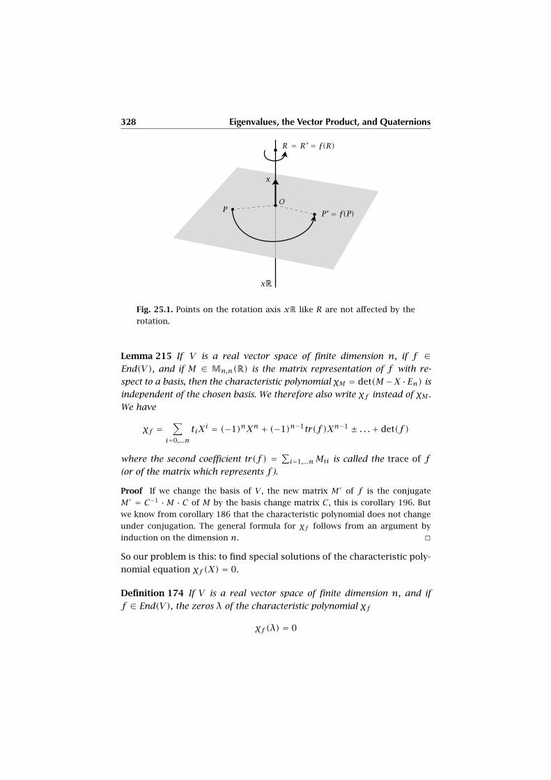
328 Eigenvalues, the Vector Product, and Quaternions
Fig. 25.1. Points on the rotation axis xR like R are not affected by the
rotation.
Lemma 215 If V is a real vector space of finite dimension n, if f ∈End(V), and if M ∈ Mn,n(R) is the matrix representation of f with re-
spect to a basis, then the characteristic polynomial χM = det(M−X ·En) is
independent of the chosen basis. We therefore also write χf instead of χM .
We have
χf =∑
i=0,...n
tiXi = (−1)nXn + (−1)n−1tr(f )Xn−1 ± . . .+ det(f )
where the second coefficient tr(f ) = ∑i=1,...nMii is called the trace of f
(or of the matrix which represents f ).
Proof If we change the basis of V , the new matrix M ′ of f is the conjugate
M′ = C−1 ·M · C of M by the basis change matrix C , this is corollary 196. But
we know from corollary 186 that the characteristic polynomial does not change
under conjugation. The general formula for χf follows from an argument by
induction on the dimension n. �
So our problem is this: to find special solutions of the characteristic poly-
nomial equation χf (X) = 0.
Definition 174 If V is a real vector space of finite dimension n, and if
f ∈ End(V), the zeros λ of the characteristic polynomial χf
χf (λ) = 0
25.1 Eigenvalues and Rotations 329
are called the eigenvalues of f . The non-zero elements x of the non-trivial
kernel Ker(f − λ · IdV ) for an eigenvalue λ are called eigenvectors of f
(corresponding to λ). They are characterized by f(x) = λx.
Remark 29 In the case where all eigenvalues of f are real, i.e., λi ∈ R
for all i, the corresponding eigenvectors form a basis of Rn, and in this
basis the matrix of f is diagonal, where the diagonal elements are the
eigenvalues.
We are more concretely interested in the case dim(V) = 3, where we have
the polynomial
χf = −X3 + tr(f )X2 + t1X + det(f ),
and we are looking for solutions λ such that−λ3+tr(f )λ2+t1λ+det(f ) =0. It will be shown in the second volume of this book that every polyno-
mial P ∈ R[X] of odd degree has at least one root in R. Therefore, the
characteristic polynomial has a real eigenvalue λ0. Let us show that in the
case of f ∈ SO(V), there is a positive eigenvalue. The equation factorizes
to
−X3 + tr(f )X2 + t1X + det(f ) = −X3 + tr(f )X2 + t1X + 1
= −(X − λ0)(X2 + bX + c)
= −X3 + (λ0 − b)X2 + (λ0b − c)X + λ0c
and therefore λ0 ·c = 1. If λ0 < 0, then c < 0, and then we have two more
real solutions λ1,2 = −b±√b2−4c2 since b2 − 4c ≥ 0, and square roots of
non-negative elements exist in R (see corollary 90 in chapter 9). Therefore
1 = λ0λ1λ2, which means that one of these solutions must be positive.
So, after renaming the roots, we take a positive eigenvalue λ0 and look
at a corresponding eigenvector x, i.e., f(x) = λ0x. Since f is an isom-
etry, we have ‖f(x)‖ = |λ0|‖x‖ = ‖x‖, whence λ0 = 1, and we have a
1-dimensional subspace Rx which is left pointwise fixed under f . This
shows:
Proposition 216 Every rotation f ∈ SO(V) for an Euclidean space (V , b)
with dim(V) = 3, has a rotation axis Af = Rx, i.e., f |Af = IdAf . If f ≠ IdV ,
the rotation axis is unique.
Proof The only open point here is uniqueness of a rotation axis. But if we had
two rotation axes, the plane H generated by these axes would be fixed pointwise,
330 Eigenvalues, the Vector Product, and Quaternions
so H⊥ would have to be reflected or remain unchanged. In both cases, this would
not yield a non-trivial transformation in SO(V). �
Since Af ⊕ A⊥f∼→ V , the isometry f which leaves the rotation axis point-
wise invariant also leaves invariant the 2-dimensional orthogonal plane
A⊥f , i.e., each point of A⊥f is mapped to another point of A⊥f . Taking an
orthonormal basis (a1, a2) of A⊥f , we may rewrite f in terms of the or-
thonormal basis (a0, a1, a2), a0 = x/‖x‖ as a matrix
Mf =
1 0 0
0 cos(θ) − sin(θ)
0 sin(θ) cos(θ)
which makes explicit the rotation in the plane A⊥f orthogonal to the ro-
tation axis Af . This representation is unique for all orthonormal bases
(a′0, a′1, a
′2) of same orientation, which represent the orthogonal decom-
position defined by the rotation axis, i.e., Af = Ra′0 and A⊥f = Ra′1+Ra′2.
The above formula and the invariance of the trace tr(f ) with respect to
basis changes implies this uniqueness result:
Corollary 217 Every rotation in SO(V) for an Euclidean space (V , b) with
dim(V) = 3, has a rotation angle θ whose cos(θ) is uniquely determined,
i.e.,
cos(θ) = 1
2(tr(f )− 1).
So we are left with the elements f ∈ O−(V) for dim(V) = 3. There are
two cases for the characteristic polynomial:
1. Either it has a positive solution λ0 = 1, then we have again a rotation
axis Af and the orthogonal complement is left invariant not by a ro-
tation, but by a reflection at a line Bf ∈ A⊥f . This line and the axis Afare left point-wise invariant, whereas the orthogonal complement line
C = B⊥f in A⊥f is inverted by −1. This means that f is a reflection ρH
at the plane H generated by Af and Bf .
2. Or else, there is no positive eigenvalue. Then we have the eigenvalue
−1 and an eigenvector x with f(x) = −x. Then the reflection ρH at
the planeH = x⊥ yields an isometry g = ρH◦f ∈ SO(V), with rotation
axis Ag = Rx. Therefore, f = ρH ◦ g is the composition of a rotation
g and a reflection ρH orthogonal to the rotation axis of g.
So this classification covers all cases of isometries in O(V),dim(V) = 3.

25.2 The Vector Product 331
25.2 The Vector Product
If we are given a triple (x1, x2, x3) of vectors xi ∈ V in a Euclidean space
(V , b) of dimension 3, and if (ei) is an orthonormal basis of V , then the
linear map f : ei , xi has a determinant det(f ), which we also write as
det(ei)(x1, x2, x3). We know that this determinant does only depend on
the orientation defined by (ei). So if we fix the orientation ω of (ei), we
have a function detω(x1, x2, x3). In the basis (ei), The columns of Mf ,
the matrix of f , are the vectors x1, x2 and x3, therefore we can deduce
the following properties from the general properties of the determinant
described in theorem 181 of chapter 20:
1. The function detω(x1, x2, x3) is linear in each argument.
2. The function is skew-symmetric, i.e., detω(x1, x2, x3) = 0 if two of
the three xi are equal. This entails that detω(xπ(1), xπ(2), xπ(3)) =sig(π)detω(x1, x2, x3) for a permutation π ∈ S3.
3. detω(x1, x2, x3) = 1 for any orthonormal basis (x1, x2, x3) ∈ω.
Therefore we define the vector product as follows:
Definition 175 Given a 3-dimensional Euclidean space (V , b), with the
previous notations, fix a pair (x1, x2) of vectors in V . Then under the iso-
morphism ∗b : V∼→ V∗, the linear form
d(x1,x2) ∈ V∗ defined by d(x1,x2)(x) = detω(x1, x2, x)
corresponds to a vector (∗b)−1d(x1,x2) ∈ V which we denote by x1 ∧ x2,
and which is characterized by the equation
b(x1 ∧ x2, x) = detω(x1, x2, x),
and which is called the vector product of x1 and x2 (in this order).1 The
orientation ω is not explicitly denoted in the vector product expression,
but should be fixed in advance, otherwise the product is only defined up to
sign.
Given the representations x1 =∑i x1iei and x2 =
∑i x2iei, the vector
product has these coordinates in terms of the basis (ei):
1 Some texts also use the notation x1 × x2 instead of x1 ∧ x2.

332 Eigenvalues, the Vector Product, and Quaternions
(x1 ∧ x2)1 = x12x23 − x13x22,
(x1 ∧ x2)2 = x13x21 − x11x23,
(x1 ∧ x2)3 = x11x22 − x12x21.
From the definition, it follows that x1 ∧ x2 is linear in each argument and
skew-symmetric, i.e., x1 ∧ x2 = −x2 ∧ x1.
Exercise 128 Show that (x ∧ y)⊥x and (x ∧ y)⊥y . Calculate e2 ∧ e1
for two basis vectors of an orthonormal basis (e1, e2, e3) of the given
orientation.
Exercise 129 Calculate the vector product (1,−12,3) ∧ (0,3,6) of two
vectors in R3 with the standard scalar product b = (?, ?) and the orienta-
tion of the standard basis (e1 = (1,0,0), e1 = (0,1,0), e1 = (0,0,1)).
Proposition 218 Given a 3-dimensional Euclidean space (V , b) with a
fixed orientation, the vector product satisfies these identities for any three
vectors u,v and w:
(i) u∧ (v ∧w) = b(u,w)v − b(u,v)w ,
(ii) (Jacobi Identity) u∧ (v ∧w)+ v ∧ (w ∧u)+w ∧ (u∧ v) = 0.
Proof Since the expressions in question are all linear in each argument, it suffices
to verify them for u = ei, v = ej ,w = ek, i, j, k = 1,2,3, where e1, e2, e3 is an
orthonormal basis. Further, (i) is skew-symmetric in v andw whence some cases
can be omitted. We leave to the reader the detailed verification, which follows
from the formulas given in this section for the coordinatewise definition of the
vector product. �
Fig. 25.2. The parallelepiped spanned by the vectors x, y and z.

25.3 Quaternions 333
Remark 30 We should add a remark on surfaces of parallelograms and
volumes of parallelepipeds which have not yet been defined and which
belong to the chapters on calculus in the second volume of this book.
However, from high school the reader may temporarily recall the defi-
nitions of surfaces and volumes and read these remarks which will be
fully justified later. If we are given x,y, z ∈ V , a Euclidean space of di-
mension 3, then we can consider the parallelogram spanned by x and y ,
i.e., the set Parallel(x,y) = {t | t = λx + µy,0 ≤ λ, µ ≤ 1} as well as
the parallelepiped spanned by x, y and z, i.e., the set Parallel(x,y, z) ={t | t = λx + µy + νz,0 ≤ λ, µ, ν ≤ 1}. The surface of Parallel(x,y) is
|x∧y|, whereas the volume of Parallel(x,y, z) is |b(x∧y,z)|, and these
numbers are independent of the orientation.
25.3 Quaternions
We have learned that 2-dimensional rotations are essentially products of
complex numbers of norm 1. We shall see in this section that in three
dimensions, we also have an algebraic structure, the quaternions, which
can be used to describe rotations in three dimensions. It seems that there
is a deep relation between algebra and geometry, a relation which is clas-
sical in algebraic geometry, but which turns out to become more intense
for the groups of transformations in linear geometry. It is not by chance
that this field of research is named geometric algebra.
The quaternions were invented by the mathematician William Rowan
Hamilton (1805–1865), who was in search for a correspondence to the
geometric interpretation of complex numbers for three dimensions. Al-
though quaternions were overrated by the so-called “quaternionists”
(see [12]) as being a kind of magic objects, they are firmly established
in computer graphics and also in aerospace science (see [35]).
Let us first motivate how quaternions relate to the vector product. As
is shown by the Jacobi identity in proposition 218, the anticommutative
(i.e., x ∧ y = −y ∧ x) vector product is not associative. In particular,
0 = (x ∧ x) ∧ y , while x ∧ (x ∧ y) may be different from 0. Quater-
nions were invented while looking for the construction of an algebraic
multiplication structure which is associative, such that the square of an
element x cannot be annihilated (as it happens with the vector product,
since always x∧x = 0). As already seen with the complex numbers, such

334 Eigenvalues, the Vector Product, and Quaternions
a desideratum may be met by adding supplementary dimensions to the
given space. Hamilton’s solution was to add one dimension to the three
dimensions of R3 and to delegate the non-vanishing part of the square to
that new dimension. His philosophical justification of this procedure was
that the three space coordinates must be supplemented by one time coor-
dinate to describe the comprising four-dimensional space-time. It is not
by chance (recall the definition of the vector product, which is intimately
related to the bilinear form of the Euclidean space) that the new compo-
nent of the Hamilton product of u,v ∈ R3 was just the negative of the
scalar product −(u,v). There is in fact nothing arbitrary in Hamilton’s
construction. It can not only be shown that C is the only field of dimen-
sion two over the reals, but that the set of quaternions H is the only skew
field of dimension four over the reals! Here is the formal definition:
Definition 176 The quaternions are a skew field H (for Hamilton), whose
additive group is R4, and whose multiplication is defined as follows. One
identifies R4 with the direct sum R ⊕ R3 defined by the projections R :
H → R : (r , x,y, z) , r and P : H → R3 : (r , x,y, z) , (x,y, z), such
that every q ∈ H is uniquely decomposed as q = r + p with r = R(q) ∈R(H)
∼→ R and p = P(q) ∈ P(H) ∼→ R3. The summand p is called the pure
part of q, and if r = 0,then q is called a pure quaternion. The summand r
is called the real part of q, and if p = 0, then q is called a real quaternion.
If the context is clear, the additive notation q = r + p is always meant in
this understanding.2 The pure part is provided with the standard scalar
product (?, ?) in R3, together with the orientation given by the canonical
basis ((1,0,0), (0,1,0), (0,0,1)). The quaternion product is now defined
by
(r + p) · (r ′ + p′) = (r · r ′ − (p,p′))+ (r · p′ + r ′ · p + p ∧ p′),
i.e.,
R((r + p) · (r ′ + p′)) = r · r ′ − (p,p′),and
P((r + p) · (r ′ + p′)) = r · p′ + r ′ · p + p ∧ p′.On H, conjugation is defined by ? : H → H : q = r + p , q = r − p. The
norm ‖q‖ of a quaternion q is defined by
‖q‖ =√q · q,
2 Remember remark 25 concerning addition in direct sums.
25.3 Quaternions 335
which makes sense since q · q = r 2 + (p,p) is a non-negative real quater-
nion, which coincides with the square norm of q when interpreted in the
standard Euclidean space (R4, (?, ?)).
The immediate properties of H, in particular the skew field properties,
are summarized in the following sorite:
Sorite 219 Let q, q′ ∈ H be quaternions. Then
(i) Conjugation ? : H → H is a linear anti-involution, i.e., q = q and
q · q′ = q′ · q.
(ii) q = q iff q is real, i.e., q = R(q).(iii) q = −q iff q is pure, i.e., q = P(q).(iv) q is pure iff q2 is a real number ≤ 0.
(v) q is real iff q2 is a real number ≥ 0.
(vi) We have ‖q · q′‖ = ‖q‖ · ‖q′‖.(vii) With the quaternion product,H becomes a skew field with 1H = 1+0.
The inverse of q ≠ 0 is the quaternion q−1 = 1‖q‖2q.
(viii) The injection R → H : r , r · 1H identifies the subfield R of real
quaternions, which commutes with all quaternions, i.e., r · q = q · rfor all r ∈ R, q ∈ H. Conversely, if q′ · q = q · q′ for all q, then q′ is
real.
(ix) By linearity in each factor, the multiplication x · y on H is entirely
determined by the following multiplication rules for the four basis
vectors 1H, i, j, k. Observe that i, j, k are pure and, therefore, their
vector product is defined.
1H · t = t · 1H = t for all t = 1H, i, j, k,
i2 = j2 = k2 = −1H,
ij = −ji = i∧ j = k,jk = −kj = j ∧ k = i,ki = −ik = k∧ i = j.
The permutation (i, j, k) induces an automorphism of H.
(x) Setting i = (0,1,0,0), j = (0,0,1,0), k = (0,0,0,1), the three injec-
tions
336 Eigenvalues, the Vector Product, and Quaternions
(i) : C→ H : a+ ib , a+ ib,(j) : C→ H : a+ ib , a+ jb,(k) : C→ H : a+ ib , a+ kb
define identifications of the field C with the subfields R + iR,R +jR,R + kR, respectively, which are related with each other by the
automorphism of H induced by the permutation (i, j, k).
(xi) We have (q, q′) = 12(qq
′ + q′q).Proof For (i) and a quaternion q = r + p, we have q = (r − p) = r − (−p) =r + p = q. And for q′ = r ′ + p′, we have
q · q′ = (r · r ′ − (p,p′))+ (r · p′ + r ′ · p + p ∧ p′)= (r · r ′ − (p,p′))− (r · p′ + r ′ · p + p ∧ p′)= (r ′ · r − (p′, p))+ (r · (−p)+ r ′ · (−p′)+ p′ ∧ p)= q′ · q
Points (ii) and (iii) are obvious.
For (iv), we have this general formula: q2 = (r 2 − (p,p)) + 2rp. If q = p, then
q · q = −‖p‖2 ≤ 0. Conversely, if r ≠ 0, then if p ≠ 0, P(q2) = 2rp ≠ 0. If q is
real, then q2 = r 2 > 0.
The proof of point (v) proceeds along the same straightforward calculation, we
therefore leave it as an exercise for the reader.
Next, we prove (viii). The commutativity of real quaternions with all quaternions
is immediate from the definition of the quaternion product. Conversely, if q·q′ =q′ ·q for all q′, then p∧p′ = p′∧p = −p∧p′ = 0 for all p′. But for p ≠ 0, taking
p,p′ linearly independent yields a contradiction, so p = 0.
As to (vi), ‖q · q′‖ =√q · q′ · q · q′ =
√q · q′ · q′ · q =
√q · ‖q′‖2 · q, but
real quaternions commute with all quaternions by (viii), so√q · ‖q′‖2 · q =√
‖q′‖2 · q · q =√‖q′‖2 · ‖q‖2 = ‖q′‖ · ‖q‖, and we are done.
Next, we prove (ix). The first point is R-linearity in each argument. But in view of
the defining formula of multiplication, this follows from linearity of the scalar
product (?, ?) and of the vector product ∧. The permutation (i, j, k) of the basis
(1H is fixed) transforms the equation i · j = k into j ·k = i and this into k · i = j,and this latter into the first, furthermore i2 = j2 = k2 = −1 is invariant under all
permutations of i, j, k, and so are the products with 1H.
Point (vii) is straightforward, except that we must verify associativity. This fol-
lows from the associativity of multiplication rules for the basis (1H, i, j, k) in
(ix), since multiplication is R-linear in each factor. The reader should verify all
equalities x · (y · z) = (x · y) · z for three arbitrary basis elements, but should
also use the permutation (i, j, k) to minimize the cases to be studied.
25.3 Quaternions 337
Point (x) is obvious.
Point (xi) is an immediate consequence of the definition of the product. �
We have now established all the necessary algebraic ingredients to tackle
the promised geometric features. To this end, recall that we have a group
isomorphism of SO2(R) (the special orthogonal group of R2) and the mul-
tiplicative group U ⊂ C of complex numbers of norm 1, i.e., the unit cir-
cle U = S(C) = {z | ‖z‖ = 1}. Therefore we suggest to consider the
group S(H) = {q | ‖q‖ = 1} of unit quaternions (in a Euclidean space,
this subset is called the unit sphere). This is a group because of point
(vi) in sorite 219. The relation between quaternion multiplication and 3-
dimensional isometries is this:
Proposition 220 Let s, s′ ∈ H∗ be non-zero quaternions.
(i) If s ∈ P(H) is pure, then the map q , −s · q · s−1 leaves the pure
quaternion space P(H) invariant and its restriction to P(H) is the
reflection ρs⊥ in P(H) at the plane s⊥ orthogonal to s.
(ii) The map q , Ints(q) = s · q · s−1 leaves the pure quaternion
space P(H) invariant, and its restriction IntPs to P(H) is a rotation
in SO3(R).
(iii) We have IntPs = IntPs′ iff Rs = Rs′.(iv) The restriction IntPSs of the map IntPs to arguments s in the unit
sphere S(H) is a surjective group homomorphism
IntPS? : S(H)→ SO3(R)
with kernel Ker(IntPS) = {±1}.Proof (i) By criterion (iv) in sorite 219, we suppose q2 is a real number ≤ 0. So
(±s ·q ·s−1)2 = s ·q2 ·s−1 = q2 is also real and ≤ 0, i.e., ±s ·q ·s−1 is pure. These
maps are evidently R-linear. Since ‖ ± s · q · s−1‖ = ‖s‖ · ‖q‖ · ‖s‖−1 = ‖q‖, the
maps q , ±s · q · s−1 conserve norms and therefore their restrictions to P(H)
are in O3(R). Now, if s is pure, then −s · s · s−1 = −s, whereas for a pure q⊥s,by (xi) we have 0 = (q, s) = 1
2(q · s + s · q) = −12 (q · s + s · q), i.e., −q · s = s · q,
whence −s · q · s−1 = q · s · s−1 = q, and therefore the plane s⊥ orthogonal to s
remains fixed, i.e., q , −s · q · s−1 on P(H) is a reflection at s⊥.
(ii) For any quaternion s the map IntPs ∈ O3(R), because
(sqs−1, sq′s−1) = 1
2(sqs−1 · sq′s−1 + sq′s−1 · sq′s−1)
= 1
2(s−1 · sq · sq′s−1 + s−1 · sq′ · sqs−1)
338 Eigenvalues, the Vector Product, and Quaternions
= 1
2(s−1 · q · s · sq′s−1 + s−1 · q′ · s · sqs−1)
= 1
2(s
‖s‖2q · (‖s‖2s−1) · sq′s−1 + s
‖s‖2q′ · (‖s‖2s−1) · sqs−1)
= 1
2(sqs−1 · sq′s−1 + sq′s−1 · sqs−1)
= 1
2s(qq′ + q′q)s−1
= 1
2(qq′ + q′q)
= (q, q′)
The map Ints for a real s is the identity, so suppose s is not real. Consider for
µ ∈ [0,1], the real unit interval, the quaternion sµ = (1 − µ) + µ · s, so s0 =1, s1 = s, and sµ ≠ 0 for all µ ∈ [0,1]. So IntPsµ ∈ O3(R) for all µ ∈ [0,1],i.e., f(µ) = det(IntPsµ ) is never zero, and it is always ±1. We shall show in the
chapter on topology in volume II of this book, that f has the property of being
continuous (a concept to be introduced in that chapter). Evidently, f(0) = 1. On
the other hand, if we had f(1) = −1, then by continuity of f , there would exist
µ ∈ [0,1] with f(µ) = 0, a contradiction, so IntPs ∈ SO3(R).
(iii) If s′ = λs, λ ∈ R∗, then s′ · q · s′−1 = λs · q · λ−1s−1 = s · q · s−1. Conversely,
if IntPs′ = IntPs , then −IntPs′ = −IntPs , so the rotation axis Rs = Rs′ is uniquely
determined.
As to (iv), the map IntPS is a group homomorphism, since (s′ · s) · q · (s′ · s)−1 =s′ · s · q · s−1 · s′−1. It is surjective, since every rotation is the product of an
even number of reflections at hyperplanes (see proposition 208). So since the
reflections are represented by the quaternion multiplications −s · q · s−1 by (i),
rotations are represented by the product of an even number of such reflections
which yields the required map. Since two rotations are equal iff their quaternions
s define the same line Rs, and since any line has exactly two points t,−t on the
sphere S(H), the kernel is {±1}. �
So we recognize that rotations in SO3(R) can be described by conjuga-
tions IntPSs with quaternions, and the composition of rotations corre-
sponds to the conjugation of products. This is exactly what was expected
from the 2-dimensional case of complex multiplication. The identifica-
tion of the quotient group S(H)/{±1} and SO3(R) gives us an interesting
geometric interpretation of SO3(R): Observe that each line R · x ⊂ R3
intersects the unit sphere S(R3) exactly in two points s,−s of norm 1.
These points are identified via the two-element group {±1}. So the quo-
tient group identifies with the set P3(R) of lines through the origin (1-
dimensional subspaces) in R4. This space is called the three-dimensional
projective space of R3. So we have this corollary:
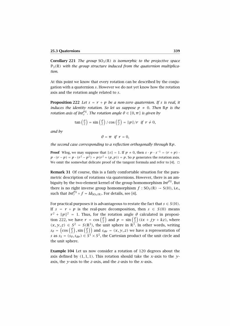
25.3 Quaternions 339
Corollary 221 The group SO3(R) is isomorphic to the projective space
P3(R) with the group structure induced from the quaternion multiplica-
tion.
At this point we know that every rotation can be described by the conju-
gation with a quaternion s. However we do not yet know how the rotation
axis and the rotation angle related to s.
Proposition 222 Let s = r + p be a non-zero quaternion. If s is real, it
induces the identity rotation. So let us suppose p ≠ 0. Then Rp is the
rotation axis of IntPSs . The rotation angle θ ∈ [0, π] is given by
tan(θ2
)= sin
(θ2
)/ cos
(θ2
)= ‖p‖/r if r 6= 0,
and by
θ = π if r = 0,
the second case corresponding to a reflection orthogonally through Rp.
Proof Wlog, we may suppose that ‖s‖ = 1. If p ≠ 0, then s · p · s−1 = (r + p) ·p · (r −p) = p · (r 2 −p2) = p(r 2+ (p,p)) = p. So p generates the rotation axis.
We omit the somewhat delicate proof of the tangent formula and refer to [4]. �
Remark 31 Of course, this is a fairly comfortable situation for the para-
metric description of rotations via quaternions. However, there is an am-
biguity by the two-element kernel of the group homomorphism IntPS . But
there is no right inverse group homomorphism f : SO3(R) → S(H), i.e.,
such that IntPS? ◦ f = IdSO3(R). For details, see [4].
For practical purposes it is advantageous to restate the fact that s ∈ S(H).If s = r + p is the real-pure decomposition, then s ∈ S(H) means
r 2 + ‖p‖2 = 1. Thus, for the rotation angle θ calculated in proposi-
tion 222, we have r = cos(θ2
)and p = sin
(θ2
)(ix + jy + kz), where
(x,y, z) ∈ S2 = S(R3), the unit sphere in R3. In other words, writing
sθ =(cos
(θ2
), sin
(θ2
))and sdir = (x,y, z) we have a representation of
s as sS = (sθ, sdir) ∈ S1 × S2, the Cartesian product of the unit circle and
the unit sphere.
Example 104 Let us now consider a rotation of 120 degrees about the
axis defined by (1,1,1). This rotation should take the x-axis to the y-
axis, the y-axis to the z-axis, and the z-axis to the x-axis.
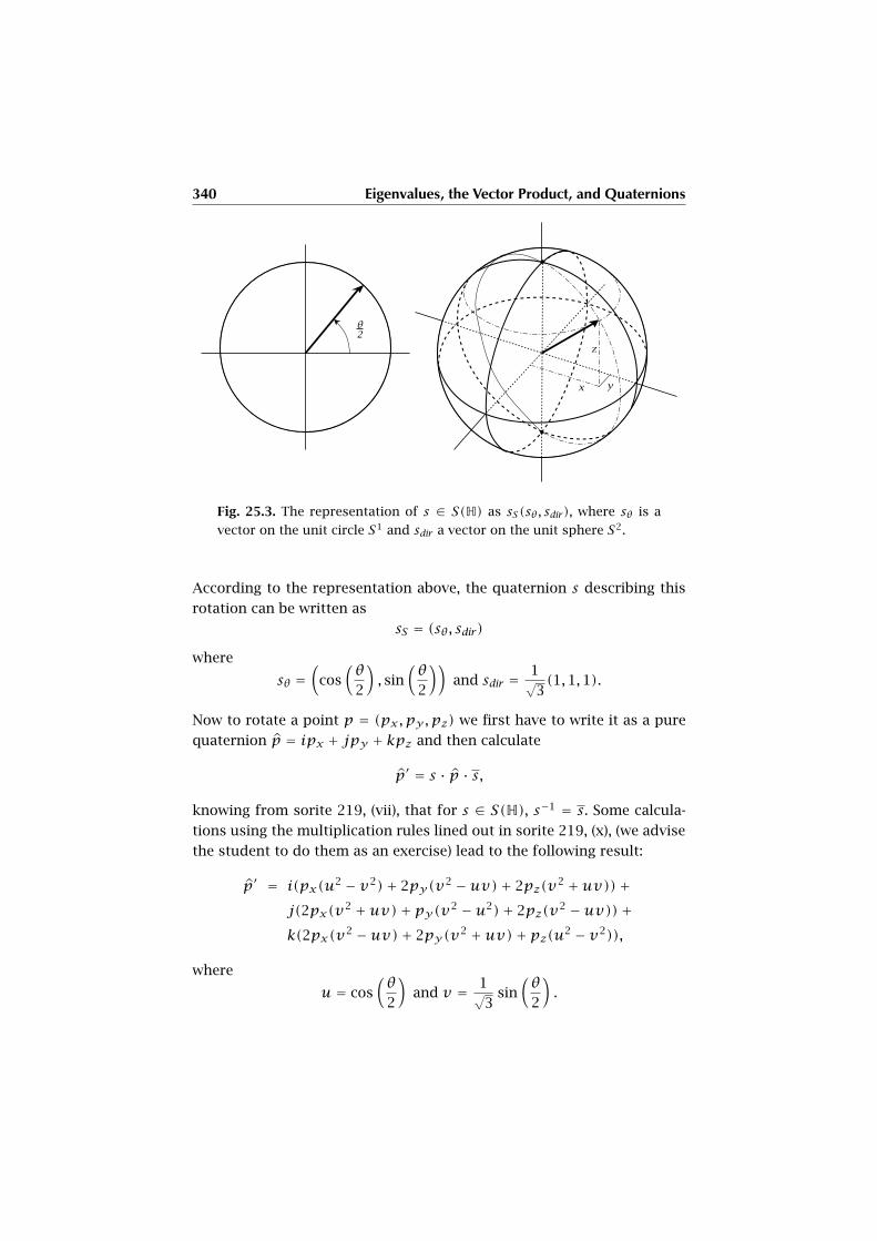
340 Eigenvalues, the Vector Product, and Quaternions
Fig. 25.3. The representation of s ∈ S(H) as sS(sθ , sdir), where sθ is a
vector on the unit circle S1 and sdir a vector on the unit sphere S2.
According to the representation above, the quaternion s describing this
rotation can be written as
sS = (sθ, sdir)
where
sθ =(
cos(θ
2
), sin
(θ
2
))and sdir = 1√
3(1,1,1).
Now to rotate a point p = (px , py , pz) we first have to write it as a pure
quaternion p = ipx + jpy + kpz and then calculate
p′ = s · p · s,
knowing from sorite 219, (vii), that for s ∈ S(H), s−1 = s. Some calcula-
tions using the multiplication rules lined out in sorite 219, (x), (we advise
the student to do them as an exercise) lead to the following result:
p′ = i(px(u2 − v2)+ 2py(v
2 −uv)+ 2pz(v2 +uv))+
j(2px(v2 +uv)+ py(v2 −u2)+ 2pz(v
2 −uv))+k(2px(v
2 −uv)+ 2py(v2 +uv)+ pz(u2 − v2)),
where
u = cos(θ
2
)and v = 1√
3sin
(θ
2
).
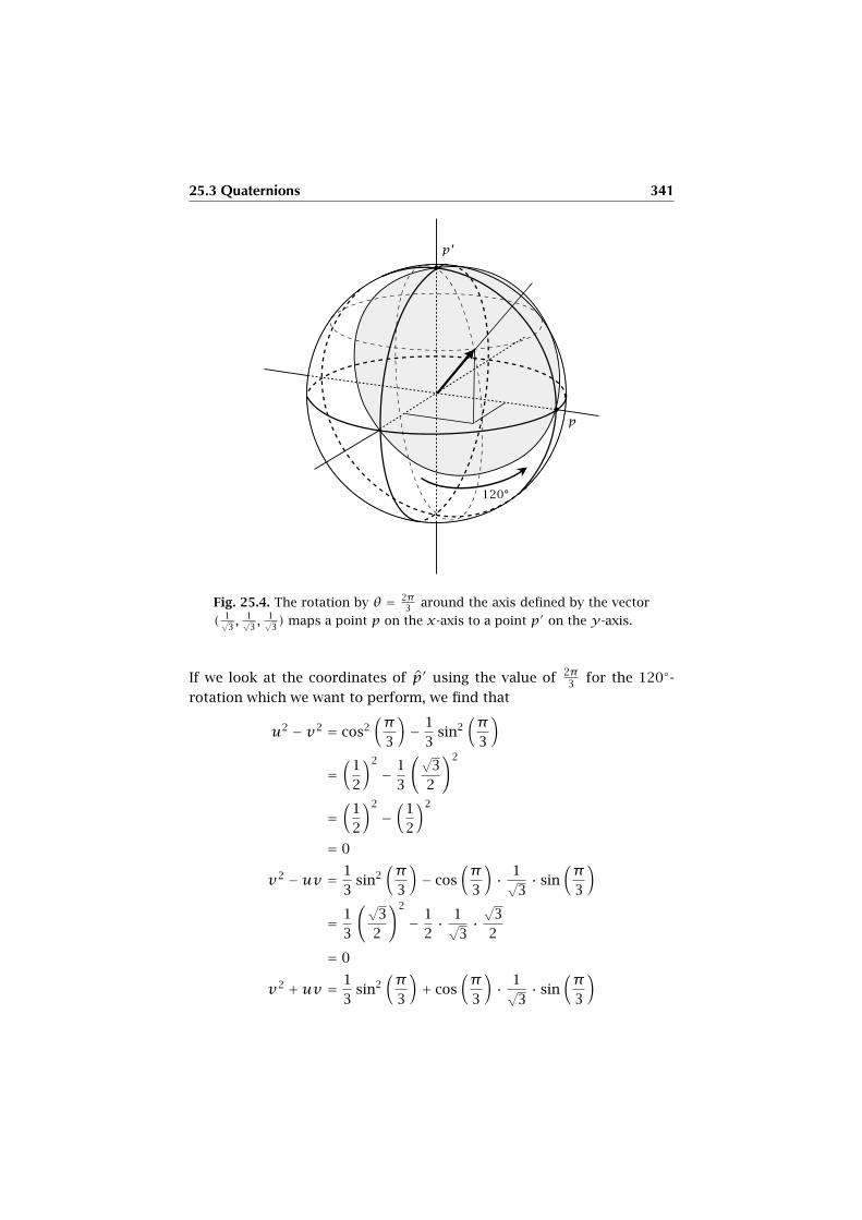
25.3 Quaternions 341
Fig. 25.4. The rotation by θ = 2π3 around the axis defined by the vector
( 1√3 ,
1√3 ,
1√3) maps a point p on the x-axis to a point p′ on the y-axis.
If we look at the coordinates of p′ using the value of 2π3 for the 120◦-
rotation which we want to perform, we find that
u2 − v2 = cos2(π
3
)− 1
3sin2
(π
3
)
=(
1
2
)2
− 1
3
(√3
2
)2
=(
1
2
)2
−(
1
2
)2
= 0
v2 −uv = 1
3sin2
(π
3
)− cos
(π
3
)· 1√
3· sin
(π
3
)
= 1
3
(√3
2
)2
− 1
2· 1√
3·√
3
2
= 0
v2 +uv = 1
3sin2
(π
3
)+ cos
(π
3
)· 1√
3· sin
(π
3
)
342 Eigenvalues, the Vector Product, and Quaternions
= 1
3
(√3
2
)2
+ 1
2· 1√
3·√
3
2
= 1
2
Here we use the trigonometric facts that sin(π3 ) =√
32 , and cos(π3 ) = 1
2 .
Putting this together again, we get
p′ = ipz + jpx + kpy
and for p = (1,0,0) we do indeed get p′ = (0,1,0).
CHAPTER 26
Second Advanced Topic
In this second advanced chapter, we shall briefly describe the theory of
finite fields, called Galois fields, and then give two important applications
of this theory: The first is Reed’s and Solomon’s error correction code,
which is of great importance in media encoding for CDs, DVDs, ADSL,
etc. The second is the encryption algorithm developed by Rivest, Shamir
and Adleman, which is of practical use in digital signature generation, for
example.
26.1 Galois Fields
Galois fields are by definition commutative fields with finite cardinality.
(In field theory, it can be shown that every finite skew field is in fact
automatically commutative, so no other finite fields exist.) Their name
has been chosen in honor of the French mathematician Evariste Galois
(1811–1832), who invented the algebraic theory of polynomial equations
and thereby was, among others, able to solve some of the most difficult
questions in mathematics: The conjecture of the impossibility of a gener-
ally valid construction by compass and straightedge of the trisection of
an angle or the Delian problem concerning the duplication of the cube by
the same type of construction. Unfortunately, he was killed in a duel at
the age of 20. His research had not been understood during his short life-
time. The famous mathematician Siméon-Denis Poisson commented on a
Galois paper: “His argument is neither sufficiently clear nor sufficiently
developed to allow us to judge its rigor.” Only in 1843, the mathemati-

344 Second Advanced Topic
cian Joseph Liouville recognized Galois’ work as a solution “as correct as
it is deep of this lovely problem: Given an irreducible equation of prime
degree, decide whether or not it is soluble by radicals.” This is in fact the
abstract statement implying the solution of the old problems mentioned
above.
We shall outline the theory of Galois fields, because they play a crucial
role in coding theory, the theory dealing with the methods for storing and
transmitting digital information through noisy media. In fact, bit strings
can be represented by polynomials with coefficients in Z2, which are ele-
ments of a particular Galois field. Thus we can take over the results from
the theory of Galois fields to the realm of bit strings. In the next section,
this will be exemplified by the famous Reed-Solomon error correction
code.
We start with a few definitions:
Definition 177 Let K be a field, where 0K is the additive neutral element,
and 1K is the multiplicative unit. Consider the ring homomorphism p : Z→K, with
p(n) = n · 1K = 1K + · · ·1K︸ ︷︷ ︸n times
.
The characteristic of K, denoted by char(K) is the smallest positive n, such
that p(n) = 0k. If there is no such n, then, by definition, char(K) = 0.
Definition 178 Let K be a field. The prime field of K, denoted by P(K), is
the smallest subfield of K.
Since 1K ∈ P(K), we have char(P(K)) = char(K). The following lemma
provides a classification of prime fields.
Lemma 223 Given a field K, consider the unique homomorphism of rings
p : Z→ K : n, n · 1K from definition 177.
Then Ker(p) = (char(K)) is the principal ideal generated by char(K).
There are two cases to consider:
1. Ker(p) is trivial, i.e., char(K) = 0. Then P(K) is isomorphic to Q, be-
cause it contains all integers and, being a field, all inverses of integers.
2. The characteristic char(K) > 0. Since Z/(char(K)) is a field, char(K)
is a prime by lemma 133. By proposition 124, Im(p)∼→ Z/(char(K)).
26.1 Galois Fields 345
Since P(K) = Im(p) (Im(p) ⊂ P(K), but because P(K) is minimal,
P(K) = Im(p)), we have P(K)∼→ Z/(char(K)).
Thus a Galois field (which is just another name for finite field) K has
positive prime characteristic p. Clearly, a Galois field is a vector space
over its prime field, and of finite dimension n. So, since the prime field
P(K) of K is isomorphic to Zp, we have the vector space isomorphism
K∼→ Znp , and therefore card(K) = card(Znp) = pn.
Moreover, since the group K∗ has order pn − 1, and every element a of
the group has an order which divides pn − 1, we have apn−1 = 1 (see
sorite 117 (iii)). Therefore all elements of K∗ are roots of the polynomial
Xpn−1 − 1.
Together with 0K , the elements of a field K with characteristic p and pn
elements constitute the set of roots of the polynomial X(Xpn−1 − 1) =
Xpn − X ∈ Zp[X]. Since the degree of this polynomial is pn, it has at
most pn different roots, and therefore it decomposes into a product
Xpn −X =
∏
x∈K(X − x)
of pn different linear factors. It remains to establish whether the char-
acteristic and the polynomial uniquely determine K up to field isomor-
phisms.
To this end, we sketch a short but comprehensive run through the theory
dealing with the existence and uniqueness of fields defined by roots of
certain polynomials. In all these discussions, a field extension is a pair
of fields K,L such that K ⊂ L. If K ⊂ L is such a field extension, then
L is called an extension of K. If T ⊂ L, we denote by K(T) the smallest
extension of K in L containing T and call it the extension of K generated
by T . If T = {x}, then we also write K(x) instead of K({x}).To begin with, we have the following definition:
Definition 179 If K ⊂ L is an extension and f ∈ K[X]−{0}, then x ∈ L is
called an algebraic element (over K) if f(x) = 0.
An extension K ⊂ L is called an algebraic extension if every element of L
is algebraic over K.
We have this lemma about the uniqueness of extensions.
346 Second Advanced Topic
Lemma 224 If K ⊂ L is an extension, and if x ∈ L is algebraic, then there is
a unique irreducible polynomial r = Xm+am−1Xm−1+ . . . a0 ∈ K[X] such
that the extension K(x) ⊂ L of K is isomorphic to K[X]/(r), and which,
as a K-vector space, has dimension m = deg(r), a basis being defined by
the sequence (xm−1, . . . x2, x,1). The polynomial r is called the defining
polynomial of x.
If the dimension of an extension K ⊂ L as a K-vector space is finite, then
L is algebraic over K. In particular the extension K(x) by an algebraic
element x is algebraic. If extensions K ⊂ L and L ⊂ M are algebraic, then
so is K ⊂ M .
Conversely, given an irreducible polynomial r = Xm+am−1Xm−1+. . . a0 ∈
K[X], there is an algebraic extension K ⊂ L = K(x) such that the defining
polynomial of x is r , i.e., K(x) is isomorphic to K[X]/(r).
Example 105 A Galois field K of characteristic p and dimension n is an
algebraic extension of its prime field P(X) which is isomorphic to Zp . We
have seen that every element x ∈ K is a root of a polynomial in Zp[X] (to
be precise, the polynomial Xpn −X), i.e., every element is algebraic.
Exercise 130 Show that the R ⊂ C is an algebraic extension.
Proposition 225 Consider two field extensions K ⊂ L = K(x1, x2, . . . xr )
and K′ ⊂ L′ = K′(x′1, x′2, . . . x′r ). Let k be an isomorphism k : K∼→ K′ with
this property: there is a polynomial f ∈ K[X], such that f = (X −x1)(X −x2) . . . (X − xr ) ∈ L[X], which is mapped to the polynomial f ′ ∈ K′[X]by the extension of k to the polynomial ring K[X], such that f ′ = (X −x′1)(X − x′2) . . . (X − x′r ) ∈ L′[X]. Then there is an extension l : L
∼→ L′ of
k, i.e., l|K = k.
The proof of proposition 225 is by induction on the maximal degree of
the irreducible factors in the decomposition of f in K[X], and then on
the number of such maximal degree factors. The inductive step is in fact
provided by the above lemma 224.
The next proposition ensures that every polynomial over a field K gives
rise to a field extension of K.
Proposition 226 If K is a field, and if f ∈ K[X] is a polynomial, there
exists a splitting field extension K ⊂ L of f , i.e., L = K(x1, . . . xr ) where
xi are roots of f such that in L[X], f = a(X − x1)(X − x2) . . . (X − xr ).
26.1 Galois Fields 347
The proof of this proposition is again an immediate consequence of
lemma 224. In fact, for each irreducible factor g of f in K[X], we may
embed K in the field K[X]/(g), which, by construction, contains a root of
g. And so forth until f has been split into linear factors.
We are now ready to state the main result of this section:
Corollary 227 For a given prime characteristic p and a given exponent
n > 0, there is a Galois field of the cardinality pn. It is a splitting field of
the polynomial Xpn −X, and any two such fields are isomorphic. They are
denoted by GF(pn).
Summarizing, for every prime p and every positive natural exponent n,
there is one, and, up to field isomorphisms, only one Galois field GF(pn)
of pn elements. Let us now show that in fact, GF(pn) = Zp(ζ), i.e., an
algebraic extension by a single element ζ.
Proposition 228 The multiplicative group GF(pn)∗ of a Galois field is
cyclic, i.e., isomorphic to the additive group Zpn−1. A generator ζ of this
group is called a (pn − 1)-th primitive root of unity.
The proof is easy, see [46, page 42] for details.
Therefore a Galois field GF(pn) is an algebraic extension GF(pn) = Zp(ζ)by a primitive root of unity ζ, whose defining polynomial Z ∈ Zp[X] is
of degree n, the powers 1, ζ, ζ2, . . . ζn−1 forming a basis over the prime
field. But observe that there may be different defining polynomials for
the same Galois field.
26.1.1 Implementation
We shall discuss the Reed-Solomon error correction code for the special
prime field Z2 which may be identified with the bit set Bit = {0,1} for
computerized implementation. In this case, we need to master the arith-
metics in GF(2n) on the basis of bit-wise encoding.
Identifying GF(2n) with Z2[X]/(Z), where Z is the defining polynomial of
a primitive (2n−1)-th root of unity ζ, we know that elements u ∈ GF(2n)
are uniquely represented in the basis (xn−1, . . . x2, x1,1), where x is the
image of X ∈ Z2[X] in Z2[X]/(Z) by the canonical homomorphism and
corresponds to ζ. Through the identification of GF(2n) with Z2[X]/(Z),
348 Second Advanced Topic
and the vector space identification GF(2n)∼→ Zn2 , we can identify u(x) ∈
Z2[X]/(Z) with the vector u = (un−1, . . . u2, u1, u0) ∈ Zn2 , i.e., with a bit
sequence of length n, which encodes the class of the polynomial residue
u(x) = un−1xn−1 + . . . u2x
2 +u1x +u0 in Z2[X]/(Z).
Arithmetic in this representation is as follows:
• Addition is the coordinate-wise addition of bits and has nothing to do
with the defining polynomial, except for its degree n:
(un−1, . . . u1, u0)+(vn−1, . . . v1, v0) = (un−1+vn−1, . . . u1+v1, u0+v0)
This addition may also be viewed as the logical exclusive alternative
xor on the Boolean algebra Bit = 2, via a+ b = ¬(aa b) = xor(a, b).
• Multiplication u(x) · v(x) is defined as follows:
The multiplication of u(x) by a constant ν ∈ Z2 is the coordinate-
wise multiplication of bits, i.e., corresponding to logical conjunction
a · b = a & b.
For the multiplication u(x) · x, first the residue r(x) in xn = 1 ·Z + r(x) has to be calculated. This has to be done only once for the
given n and Z. With r = (rn−1, . . . r2, r1, r0) the following two steps
are performed:
1. a shift of u = (un−1, . . . u2, u1, u0) to the left, yielding
l(u) = (un−2, . . . u1, u0,0),
2. the addition l(u)+ r in case un−1 ≠ 0.
The full multiplication u(x) ·v(x) is written as a succession of these
elementary operations (easily implemented in hardware using a shift
register, and a simple logical unit capable of & and xor operations). It
is the realization of the stepwise multiplication of u(x) by the terms
of v(x) (also known as Horner scheme):
u(x) · vn−1
(u(x) · vn−1) · x((u(x) · vn−1) · x)+ vn−2
(((u(x) · vn−1) · x)+ vn−2) · x((((u(x) · vn−1) · x)+ vn−2) · x)+ vn−3
...

26.2 The Reed-Solomon (RS) Error Correction Code 349
(. . . (u(x) · vn−1) · x) . . .)+ v0
Example 106 We consider the Galois field GF(24). It has 16 elements,
which are represented as four-bit words, e.g., u = (1,1,0,1) corresponds
to u(x) = x3 + x2 + 1. The primitive root of unity can be defined by the
polynomials Z = X4+X+1 or Z = X4+X3+1. Let us take Z = X4+X+1.
Then we have the remainder formula X4 = 1·Z+(X+1) (observe that 1 =−1 in Z2). So x4 = x + 1 in Z2[X]/(Z) which is represented as (0,0,1,1).
Therefore the multiplication u(x) · x is implemented as a left shift of u
followed by the addition of (0,0,1,1).
Exercise 131 Calculate the 16 powers xi of x for i = 1,2,3, . . .16 in the
example 106 by means of the multiplication algorithm described above.
The product in GF(pn) is also easily encoded by observing the fact that
the multiplicative group GF(pn)∗ is isomorphic to the additive group
Zpn−1. In the representation Zp[X]/(Z) of GF(pn), x is a generator, i.e.,
every non-zero element of Zp[X]/(Z) occurs as a power xi. Thus, we have
the group isomorphism ϕ : GF(pn)∗ → Zpn−1, defined by ϕ(xi) = i, and
ϕ(xixj) = i+ j. Therefore, multiplication in Zp[X]/(Z) can be replaced
by addition in Zpn−1.
As an example, the 32 − 1 = 8 elements of GF(32)∗ when represented as
elements of Zp[X]/(X3+X+1) can be calculated as the powers of x, i.e.,
by successive multiplication by x, starting with 1 (all operations are in
Zp[X]/(X3 +X + 1)):
x0 = 1, x4 = (2x + 2) · x = 2x2 + 2x,
x1 = x, x5 = (2x2 + 2x) · x = 2x2 + x + 1,
x2 = x · x = x2, x6 = (2x2 + x + 1) · x = x2 + 2x + 1,
x3 = x2 · x = 2x + 2, x7 = (x2 + 2x + 1) · x = 2x2 + 2.
26.2 The Reed-Solomon (RS) Error Correction Code
The Reed-Solomon error correction code was invented in 1960 by Lincoln
Laboratory (MIT) members Irving S. Reed and Gustave Solomon and pub-
lished in [39]. When it was written, digital technology was not advanced
enough to implement the concept. The key to the implementation of
Reed-Solomon codes was the invention of an efficient decoding algorithm
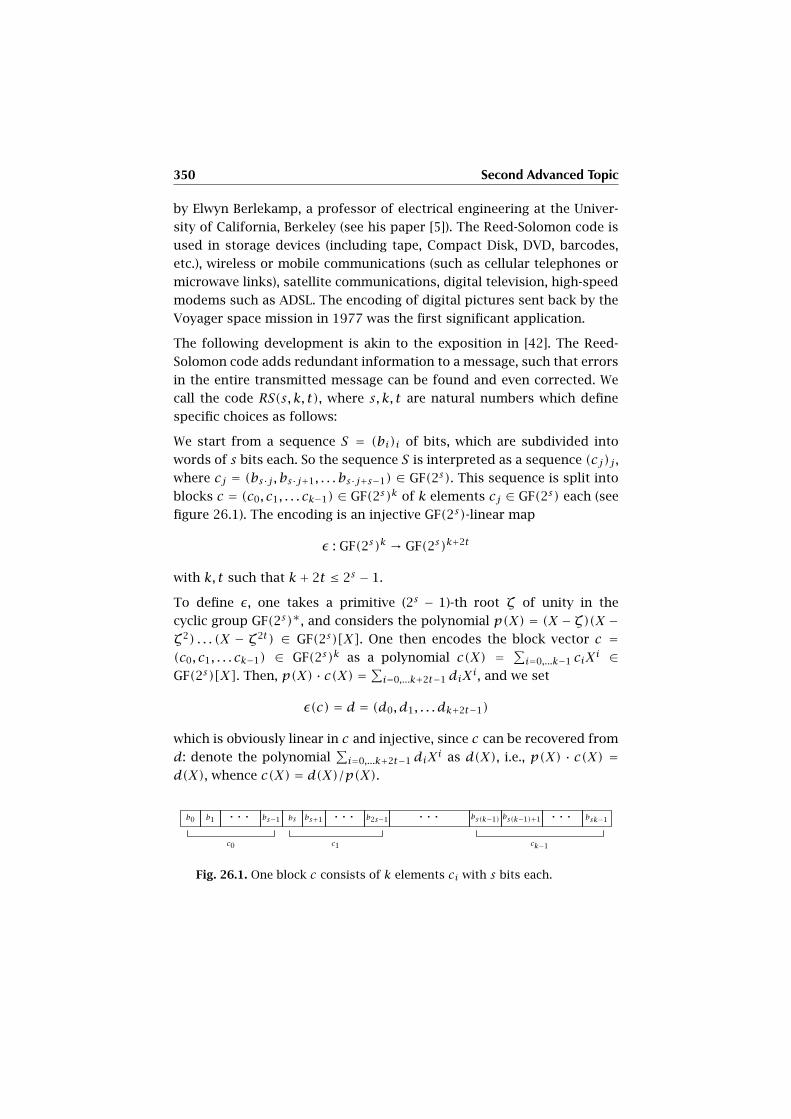
350 Second Advanced Topic
by Elwyn Berlekamp, a professor of electrical engineering at the Univer-
sity of California, Berkeley (see his paper [5]). The Reed-Solomon code is
used in storage devices (including tape, Compact Disk, DVD, barcodes,
etc.), wireless or mobile communications (such as cellular telephones or
microwave links), satellite communications, digital television, high-speed
modems such as ADSL. The encoding of digital pictures sent back by the
Voyager space mission in 1977 was the first significant application.
The following development is akin to the exposition in [42]. The Reed-
Solomon code adds redundant information to a message, such that errors
in the entire transmitted message can be found and even corrected. We
call the code RS(s, k, t), where s, k, t are natural numbers which define
specific choices as follows:
We start from a sequence S = (bi)i of bits, which are subdivided into
words of s bits each. So the sequence S is interpreted as a sequence (cj)j ,
where cj = (bs·j , bs·j+1, . . . bs·j+s−1) ∈ GF(2s). This sequence is split into
blocks c = (c0, c1, . . . ck−1) ∈ GF(2s)k of k elements cj ∈ GF(2s) each (see
figure 26.1). The encoding is an injective GF(2s)-linear map
ε : GF(2s)k → GF(2s)k+2t
with k, t such that k+ 2t ≤ 2s − 1.
To define ε, one takes a primitive (2s − 1)-th root ζ of unity in the
cyclic group GF(2s)∗, and considers the polynomial p(X) = (X − ζ)(X −ζ2) . . . (X − ζ2t) ∈ GF(2s)[X]. One then encodes the block vector c =(c0, c1, . . . ck−1) ∈ GF(2s)k as a polynomial c(X) = ∑
i=0,...k−1 ciXi ∈
GF(2s)[X]. Then, p(X) · c(X) = ∑i=0,...k+2t−1 diXi, and we set
ε(c) = d = (d0, d1, . . . dk+2t−1)
which is obviously linear in c and injective, since c can be recovered from
d: denote the polynomial∑i=0,...k+2t−1 diX
i as d(X), i.e., p(X) · c(X) =d(X), whence c(X) = d(X)/p(X).
b0 b1 · · · bs−1
c0
bs bs+1 · · · b2s−1
c1
· · · bs(k−1) bs(k−1)+1 · · · bsk−1
ck−1
Fig. 26.1. One block c consists of k elements ci with s bits each.
26.2 The Reed-Solomon (RS) Error Correction Code 351
Proposition 229 (2t-error detection) Given the above notations, if the
measured value f differs from the encoded value d in at most 2t posi-
tions, and we denote the noise e = f − d ∈ GF(2s)k+2t , then e = 0 (i.e.,
there has been no error from noise) iff (f (ζi))i=1,...2t = 0, where f(ξ) is
the evaluation of f(X) at ξ.
In fact, evaluating e(X) at ζi for all i, we have e(ζi) = f(ζi)+d(ζi), and,
since d(ζi) = 0 by construction, e(ζi) = f(ζi). This can be rewritten as
matrix equation:
(f (ζi))τ =
1 ζ ζ2 . . . ζk+2t−1
1 ζ2 ζ4 . . . ζ2(k+2t−1)
......
......
1 ζ2t ζ4t . . . ζ2t(k+2t−1)
· (ei)τ .
Now, if all ei = 0 except of at most 2t indexes i1 < i2 < . . . i2t , then the
above equation reduces to
(f (ζi))τ =
ζi1 ζi2 . . . ζi2t
ζ2i1 ζ2i2 . . . ζ2i2t
......
...
ζ2ti1 ζ2ti2 . . . ζ2ti2t
· (eij)τ = Z · (eij )τ
where (eij ) is a row vector of length 2t. But the (2t × 2t)-matrix Z of the
ζ-powers is of rank 2t, therefore Z is invertible, and we have (eij )τ =
Z−1f(ζi))τ = 0, whence the claim, that (f (ζi))i=1,...2t = 0 implies e = 0.
Let us understand why Z is regular. We have
det(Z) = ζi1+i2+···i2t · det
1 1 . . . 1
ζi1 ζi2 . . . ζi2t
ζ2i1 ζ2i2 . . . ζ2i2t
......
...
ζ(2t−1)i1 ζ(2t−1)i2 . . . ζ(2t−1)i2t
.
using the properties of the determinant presented in propostion 181. The
matrix to the right of the power of ζ is a Vandermonde matrix, whose de-
terminant is known to be∏
1≤u<v≤2t(ζiu−ζiv ). See [23] for a proof. Since
iu < k+ 2t by construction of the matrix and k+ 2t ≤ 2s − 1 by hypoth-
esis, no two powers ζiu , ζiv are equal for u ≠ v , and the Vandermonde
matrix is regular.
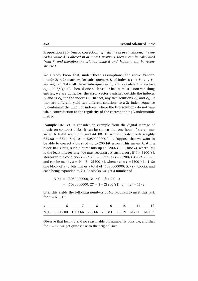
352 Second Advanced Topic
Proposition 230 (t-error correction) If with the above notations, the en-
coded value d is altered in at most t positions, then e can be calculated
from f , and therefore the original value d and, hence, c can be recon-
structed.
We already know that, under these assumptions, the above Vander-
monde 2t × 2t-matrixes for subsequences i• of indexes i1 < i2 < . . . i2tare regular. Take all these subsequences i• and calculate the vectors
ei• = Z−1i• f(ζ
i))τ . Then, if one such vector has at most t non-vanishing
entries, we are done, i.e., the error vector vanishes outside the indexes
i• and is ei• for the indexes i•. In fact, any two solutions ei′• and ei′′• , if
they are different, yield two different solutions to a 2t index sequence
i• containing the union of indexes, where the two solutions do not van-
ish, a contradiction to the regularity of the corresponding Vandermonde
matrix.
Example 107 Let us consider an example from the digital storage of
music on compact disks. It can be shown that one hour of stereo mu-
sic with 16-bit resolution and 44100 Hz sampling rate needs roughly
635MB = 635 × 8 × 106 = 5080000000 bits. Suppose that we want to
be able to correct a burst of up to 200 bit errors. This means that if a
block has s bits, such a burst hits up to d200/se + 1 blocks, where dxeis the least integer ≥ x. We may reconstruct such errors if t > d200/se.Moreover, the condition k+2t ≤ 2s−1 implies k+2d200/sek+2t ≤ 2s−1
and can be met by k = 2s −3−2d200/se, whence also t = d200/se+1. So
one block of k · s bits makes a total of d5080000000/(k · s)e blocks, and
each being expanded to k+ 2t blocks, we get a number of
N(s) = d5080000000/(k · s)e · (k+ 2t) · s= d5080000000/(2s − 3− 2d200/se) · se · (2s − 1) · s
bits. This yields the following numbers of MB required to meet this task
for s = 6 . . .12:
s 6 7 8 9 10 11 12
N(s) -5715.00 1203.66 797.66 700.83 662.19 647.66 640.63
Observe that below s ≤ 6 no reasonable bit number is possible, and that
for s = 12, we get quite close to the original size.
26.3 The Rivest-Shamir-Adleman (RSA) Encryption Algorithm 353
26.3 The Rivest-Shamir-Adleman (RSA) Encryption
Algorithm
The RSA algorithm was published in 1978 by Ron Rivest, Adi Shamir,
and Leonhard Adleman [40]. It can be used for public key encryption and
digital signatures. Its security is based on the difficulty of factoring large
integers, and again uses the theory of Galois fields.
The first step is the generation of the public and private key and runs as
follows:
1. Generate two different large primes, p and q, of approximately equal
size, such that their product n = pq is of a bit length, e.g., 1024
bits, which is required for the representation of the message as a big
number, see below in the next paragraph.
2. One computes n = pq and φ = (p − 1)(q − 1).
3. One chooses a natural number e,1 ≤ e ≤ φ, such that gcd(e,φ) = 1.
Then by definition, the couple (e,n) is the public key.
4. From the previous choice and the verification that gcd(e,φ) = 1, one
computes the inverse d,1 ≤ d ≤ φ, i.e. de = 1 mod φ. By definition,
the couple (d,n) is the private key.
5. The values p,q,φ, and d are kept secret.
The second step describes the encryption of the message sent from A to
B. The private knowledge (pB , qB ,φB) is attributed to B who will be able
to decipher the encrypted message from A.
1. B’s public key (nB , eB) is transmitted to A.
2. The message is represented by a (possibly very large) natural number
1 ≤m ≤ nB .
3. The encrypted message (the “cyphertext”) is defined by
c =meB mod nB .
4. The cyphertext c is sent to B.
Since B knows that the message number m is unique in ZnB , then once
we have recalculated m mod nB , we are done.
354 Second Advanced Topic
The third step deals with the decryption of the original message number
m by B.
1. Receiver B must use his or her private key (dB , nB) and calculate
the number cdB mod nB , where he must use the fact that m =cdB mod nB .
2. He then reconstructs A’s full message text from the numeric repre-
sentation of m.
Why is it true that m = cdB mod nB? By construction, we have cdB =meBdB =m1+s·φ in ZnB . Consider now the projection
π : Z→ ZpB × ZqB : z , (z mod pB , z mod qB)
of rings. The kernel is the principal ideal (pBqB) by the prime factor-
ization theory. So we have an injection of rings ZnB → ZpB × ZqB , and
because both rings have equal cardinality, this is an isomorphism. To
show that m = meBdB in ZnB is therefore equivalent to show this equa-
tion holds in each factor ring ZpB and ZqB . Now, if m = 0 in ZpB or
in ZqB , the claim is immediate, so let us assume that m ≠ 0 mod pB .
Then we have m = meBdB = m1msφ, and it suffices to show that
mφ =m(pB−1)(qB−1) = 1 in ZpB . This follows readily from the small Fermat
theorem 134 mpB−1 = 1 in ZpB , for m ≠ 0 mod pB . The same argument
holds for qB , and we are done.
For an in-depth treatment of cryptography, theory and implementation,
see [44] and [41].
Appendix

APPENDIX A
Further Reading
Set theory. Keith Devlin’s The Joy of Sets [20] is a modern treatment
of set theory, including non-well-founded sets. As the title indicates, the
style is rather relaxed, but the treatment is nevertheless elaborate.
Graph theory. Harris’, Hirst’s and Mossinghoff’s Combinatorics and
Graph Theory [26] includes recent results and problems that empha-
size the cross-fertilizing power of mathematics. Frank Harary’s Graph
theory [25] is a very classical book including many interesting problems
and written by one of the leading graph theorists.
Abstract algebra. Among the wealth of books on algebra, Bhattacharya’s,
Jain’s and Nagpaul’s Basic Abstract Algebra [7] is very readable. A text
with a more practical focus is Discrete Mathematics [8] by Norman Biggs.
Number theory. The branch of mathematics that deals with natural
numbers and their properties, such as primes, is called number theory.
Despite its elementary basis, number theory quickly becomes very in-
volved, with many unsolved problems. Andrews’ Number Theory [2] pro-
vides a clear introduction to the subject.
Formal logic. Alonzo Church and Willard Van Orman Quine were pio-
neers of mathematical logic. Church’s Introduction to Mathematical Logic
[15] and Quine’s Mathematical Logic [37] deal with with classical propo-
sitional and predicate logic, and their relation to set theory, with a slight
philosophical flavor. A modern text is Dirk van Dalen’s Logic and Struc-
ture [17], which also provides an exposition of natural deduction and
intuitionistic logic.
358 Further Reading
Languages, grammars and automata. Hopcroft’s, Motwani’s and Ull-
man’s Introduction to Automata Theory, Languages, and Computation [28]
provides a comprehensive exposition of formal languages and automata.
Although the theory of computation has its origin in the work of Alan
Turing and Alonzo Church, the modern treatment is much indebted to
Martin Davis’ Computability and Unsolvability [19] from 1958.
Linear algebra. Werner Greub’s Linear Algebra is a classical text, which
is written in a lucid and precise style, also extending to multilinear alge-
bra in a second volume. The two volumes Basic Linear Algebra [9] and
Further Linear Algebra [10] by Blyth and Robertson are more recent texts
for first year students, working from concrete examples towards abstract
theorems, via tutorial-type exercises. Marcel Berger’s Geometry [4] is one
of the best introductions to linear geometry, including a large number
of examples, figures, and applications from different fields, including the
arts and classical synthetic geometry.
Computer mathematics. Mathematics in the context of computers can
be roughly divided into three domains: algorithms, numerics and com-
puter algebra.
Donald Knuth’s series of The Art of Computer Programming [31, 32, 33]
has the great merit of introducing to computer science a more rigorous
mathematical treatment of algorithms such as sorting and searching or
machine arithmetic. His books have become the yardstick for all subse-
quent literature in this branch of computer science. They are, however,
not for the faint of heart. A more recent book is Cormen’s, Leiserson’s,
Rivest’s and Stein’s Introduction to Algorithms [16].
Numerics is probably the oldest application of computers, accordingly
the literature is extensive. A recent publication is Didier Besset’s Object-
Oriented Implementation of Numerical Methods [6] which exploits object-
oriented techniques.
In contrast to numerics, computer algebra focusses on the symbolic so-
lution of many of the problems presented in this book. A recent work
is von zur Gathen’s and Gerhard’s Modern Computer Algebra [47]. Com-
puter algebra is the foundation of such symbolic computation systems
as Maple or Mathematica.
APPENDIX B
Bibliography
[1] Aczel, Peter. Non-Well-Founded Sets. CSLI LN 14, Stanford, Cal. 1988.
[2] Andrews, George E. Number Theory. Dover, New York 1994.
[3] Barwise, Jon & Moss, Lawrence. Vicious Circles. CSLI Publications,
Stanford, Cal. 1996.
[4] Berger, Marcel. Geometry I, II. Springer, Heidelberg et al. 1987.
[5] Berlekamp, Elwyn. “Bit-Serial Reed-Solomon Encoders.” IEEE Trans-
actions on Information Theory, IT 28, 1982, pp. 869–874.
[6] Besset, Didier H. Object-Oriented Implementation of Numerical Meth-
ods. Morgan Kaufmann, San Francisco et al. 2001.
[7] Bhattacharya, P. B., Jain, S. K. & Nagpaul S. R. Basic Abstract Algebra.
Cambridge University Press, Cambridge 1994.
[8] Biggs, Norman L. Discrete Mathematics. Oxford University Press, Ox-
ford 2002.
[9] Blyth, Thomas S. & Robertson, Edmund F. Basic Linear Algebra.
Springer, Heidelberg et al. 2002.
[10] Blyth, Thomas S. & Robertson, Edmund F. Further Linear Algebra.
Springer, Heidelberg et al. 2001.
[11] Bornemann, Folkmar. “PRIME Is in P: A Breakthrough for ‘Every-
man’.” Notices of the AMS, vol. 50, No. 5, May 2003.
[12] Bourbaki, Nicolas. Eléments d’histoire des mathématiques. Hermann,
Paris 1969.
360 Bibliography
[13] Cap, Clemens H. Theoretische Grundlagen der Informatik. Springer,
Heidelberg et al. 1993.
[14] Chomsky, Noam. “Three models for the description of language.”
I.R.E. Transactions on information theory, volume 2, pp. 113–124, IT,
1956.
[15] Church, Alonzo. Introduction to Mathematical Logic. Princeton Uni-
versity Press, Princeton 1996.
[16] Cormen, Thomas H., Leiserson, Charles E., Rivest, Ronald L. & Stein,
Clifford. Introduction to Algorithms. MIT Press, Cambridge 2001.
[17] van Dalen, Dirk. Logic and Structure. Springer, Heidelberg et al. 1994.
[18] Date, C. J. An Introduction to Database Systems. Addison-Wesley,
Reading 2003.
[19] Davis, Martin. Computability and Unsolvability. Dover, New York
1985.
[20] Devlin, Keith J. The Joy of Sets: Fundamentals of Contemporary Set
Theory. Springer, Heidelberg et al. 1999.
[21] Goldblatt, Robert. Topoi—The Categorical Analysis of Logic. North-
Holland, Amsterdam, 1984.
[22] Greub, Werner. Linear Algebra. Springer, Heidelberg et al. 1975.
[23] Gröbner, Wolfgang. Matrizenrechnung. Bibliographisches Institut,
Mannheim 1966.
[24] Groff, James R. & Weinberg, Paul N. SQL: The Complete Reference.
McGraw-Hill Osborne, New York 2002.
[25] Harary, Frank. Graph Theory. Addison-Wesley, Reading 1972.
[26] Harris, John M., Hirst, Jeffrey L. & Mossinghoff, Michael J. Combina-
torics and Graph Theory. Springer, Heidelberg et al. 2000.
[27] Hilbert, David & Ackermann, Wilhelm. Grundzüge der theoretischen
Logik. Springer, Heidelberg et al. 1967.
[28] Hopcroft, John E., Motwani, Rajeev & Ullman, Jeffrey D. Introduction
to Automata Theory, Languages and Computation. Addison Wesley,
Reading 2000.
[29] Jensen, Kathleen & Wirth, Niklaus. PASCAL—User Manual and Report
ISO Pascal Standard. Springer, Heidelberg et al. 1974.
Bibliography 361
[30] Garey, Michael R. & Johnson, David S. Computers and Intractibility:
A Guide to the Theory of NP-Completeness. W H Freeman & Co., New
York 1979.
[31] Knuth, Donald Ervin. The Art of Computer Programming. Volume I:
Fundamental Algorithms. Addison-Wesley, Reading 1997.
[32] Knuth, Donald Ervin. The Art of Computer Programming. Volume II:
Seminumerical Algorithms. Addison-Wesley, Reading 1998.
[33] Knuth, Donald Ervin. The Art of Computer Programming. Volume III:
Sorting and Searching. Addison-Wesley, Reading 1998.
[34] Kruse, Rudolf et al. Foundations of Fuzzy Systems. John Wiley & Sons,
New York 1996.
[35] Kuipers, Jack B. Quaternions and Rotation Sequences. Princeton Uni-
versity Press, Princeton-Oxford 1998.
[36] Mac Lane, Saunders & Moerdijk, Ieke. Sheaves in Geometry and Logic.
Springer, Heidelberg et al. 1992.
[37] Quine, Willard Van Orman. Mathematical Logic. Harvard University
Press, Cambridge 1981.
[38] Rasiowa, Helena & Sikorski, Roman. The Mathematics of Metamathe-
matics. Polish Scientific Publishers, Warsaw 1963.
[39] Reed, Irving S. & Solomon, Gustave. “Polynomial Codes over Certain
Finite Fields.” Journal of the Society for Industrial and Applied Math-
ematics, Vol. 8, 1960, pp. 300–304.
[40] Rivest, Ronald L., Shamir, Adi & Adleman, Leonard A. “A method for
obtaining digital signatures and public-key cryptosystems.” Commu-
nications of the ACM, Vol. 21, Nr. 2, 1978, pp. 120–126.
[41] Schneier, Bruce. Applied Cryptography: Protocols, Algorithms, and
Source Code in C. John Wiley & Sons, New York 1996.
[42] Steger, Angelika. Diskrete Strukturen I. Springer, Heidelberg et al.
2001.
[43] Stetter, Franz. Grundbegriffe der Theoretischen Informatik. Springer,
Heidelberg et al. 1988.
[44] Stinson, Douglas R. Cryptography: Theory and Practice. CRC Press,
Boca Raton 1995.
362 Bibliography
[45] Surma, Stanislav. Studies in the History of Mathematical Logic. Polish
Academy of Sciences, 1973.
[46] van der Waerden, Bartel Leendert. Algebra I. Springer, Heidelberg et
al. 1966.
[47] von zur Gathen, Joachim & Gerhard, Jürgen. Modern Computer Alge-
bra. Cambridge University Press, Cambridge 1999.
[48] Zadeh, Lotfi A. “Fuzzy Sets.” Information and Control 8:338–363,
1965.
Index
Symbols! 35, 193n! 166(G) 181(Mij) 263(i) 335(i : M : E) 227(i : M : F ) 245(j) 335(k) 335(x,y) 29∗ 159?∗ 107, 225V∗ 311b∗ 312∗b 312+ 73, 84, 94, 160a+ 18−> 193−ab
88−x 82G/H 168a/b 870 74, 1710R 1711 74, 1711H 3351R 171G : H 169f : A 211x : A 211::= 241< 44, 53, 82, 88, 95<−> 206, 221
≤ 41= 16A= 212An 167BHLR 257E(i, j) 263En 263K(T) 345Kn 123Kn,m 123M∗ 164P(H) 334Qn 139R(H) 334R∗ 171S(C) 160S(H) 337S(EX ) 193S2 143Sn 164SAX 203t(φ) 218Tu 296R[A] 174R[X] 174[1, n] 262[n] 118[s] 42# 256#(a) 53& 193M•j 263Mi• 263C 102

364 Index
C∗ 164H 334M(R) 263M(f ) 263Mm,n(R) 263N 53P3(R) 338Q 87Q∗ 164R 93R∗ 164R+ 95R− 95⇒ 197Σ 211Z 82Z∗ 164Zn 170H\G 168⋂
20⋃17⋃nx 111
U 160, 322, 337U⊥ 314U⊥W 314x⊥y 314⊥ 196∩ 19M ·N 267· 73, 85, 94χf 328cos(θ) 323cos(f ) 322∪ 18δij 263det(M) 272detω(x1, x2, x3) 331∅ 12r ≡ s 170ηM 298ab
87GA(M) 297GF(2n) 347GF(pn) 347GL(M) 282GLn(R) 271
O(V) 313O(V ,W) 312On(R) 316SO(V) 316SO3(R) 327AX 203Adj(G) 116, 122Aff R(M,N) 297Aut(G) 163Aut(M) 162BipDi(V1, V2) 110BipDi(Γ ,∆) 133Bip(V1, V2) 114Bip(Γ ,∆) 133ComWord(A) 174CompDi(V) 109Comp(V) 114DiDi(V) 109Di(V) 114EX 193, 213End(G) 163End(M) 161End(X) 160EndR(M) 281Free(φ) 215FunType 211Fun 211Fuzzy(0,1) 199Gram(xi) 323Group(G,H) 163Id 35IdΓ 121Im(f ) 35, 283Im(x) 103IntPs 337IntPS 337IntPSs 337Ints 337Ker(f ) 283LSK(V) 133LangMachineA 250LinR(M,N) 281Loop(L) 137Loop(n) 137Monoid(M,N) 161Moore(M) 226
Index 365
Parallel(x,y) 333Path(Γ) 139Pathv(Γ) 139RS(s, k, t) 350RelType 211Rel 211Re(x) 103Ring(R, S) 172Sequ(S) 211Set(a, b) 55Stack(i, µ, E) 253Stack(i : µ : E) 253Stream(A) 224Sym(X) 160, 164Term(P) 213Turing(i, tr, sH) 257Turing(i : tr : sH) 258Word(A) 139card(a) 53codom(f ) 35deg(f ) 174deg(v) 126deg
+(v) 125deg
−(v) 125dim(M) 285dom(f ) 35gcd(a, b) 183headΓ 108lcm(a, b) 183left(w) 195lev(x) 111loga(x) 99ord(G) 166pr(a) 32, 58right(w) 195rk(M) 294round(x) 153sig(x) 168tailΓ 108tr 257tr(f ) 328value(x) 201var(x) 201xor 348∈ 15∞ 91
λ(f) 297〈S〉 162〈X〉 166R〈M〉 173R〈X1, . . . Xn〉 174C 176O 176V (A, L) 201M 217¬ 197≠ 16x ö y 1836⊂ 16∉ 15ω 331M⊕D 280⊕i=1,...nMi 281
M⊕n 280am 100q 334x 105-→? 107-→Γ 113π 323∏
87
tañ h 108
v〉 120ρH 318→ 232En
Mñ Em 268
f : a→ b 35) 211∼→ 38∼ 42sin(θ) 323sin(f ) 322t 59n√a 98√a 98
0�0 2630�n 263m�0 263⊂ 16⊊ 16∑
85

366 Index
τ 256Mτ 265τf 313τ(f) 297Γ ×∆ 129× 30×c 67> 1962 î s 202BA î s 202HA î s 202L î s 202M î φ[y] 219v î s 202î s 202|——
AX203
|——IL
204
∨ 197∧ 197x1 ∧ x2 331{} 15]0,1[ 144d(x,y) 325i 103, 335j 335k 3352V 107(ab)−1 88
2a 182f 247B(Z) 256R(D) 280ΓM 244ab 73a
1n 98ba 55f∞(I) 230
RR 280| 193a|b 86x|y 183|?| 107|Γ | 113|a| 53, 82, 96|n| 123
|x| 105|| 207‖q‖ 334‖x‖ 312@ 9RS(s, k, t) 350f 298xi 182
AAε 252An 167abelian group 163, 281ABNF 236absolute value
of integer 82of rational number 89of real number 96
absorbing 224accepted language 245accepting state 245acceptor 245
elementary graph of - 245generic - 250minimal - 251push down - 253reduced - 250simple - 249stack - 253
acceptorsequivalent - 245isomorphism of - 248morphism of - 248
Aczel, Peter 112addition 73
algorithm for - 152additive inverse
of a rational number 88of an integer 82
additive monoid 160Adjc(Γ) 116, 122adjacency matrix 116, 122, 269adjoint
linear homomorphisms 313matrix 276
adjunction 197
Index 367
Turing - 257Adleman, Leonhard 353Aff R(M,N) 297affine homomorphism 296algebra
Boolean - 196, 198Heyting - 197linear - 261logical - 192, 199monoid - 172
algebraicelement 345extension 345geometry 261
algorithm 76Euclidean - 183for addition 152
alphabetinput - 257predicative - 213propositional - 193tape - 256
alternating group 167alternative
left - 138right - 138
alternative set 45AND 5, 197angle 323ANSI 66, 228antisymmetry 26application of rules 232Archimedean ordering 89architecture of concepts 8arity 211arrow 108ASCII 228associated
digraph 113graph 113matrix of bilinear form 313power automaton 244
associativity 20atomic proposition 211attribute of sets 18Aut(G) 163
Aut(M) 162automata
isomorphism of - 248morphism of - 247
automaton 139deterministic - 244elementary graph of - 244
automorphismgroup 164of groups 163of modules 282of monoids 162of rings 172
AX 203axiom 13, 203
of choice 19, 44, 80of empty set 17of equality 17of infinity 18of pairs 18of powersets 18of subsets for attributes 18of union 17
axiomatic 13set theory 17vector space theory 262
axiomatics 203axis, rotation 327
BBHLR 257b-adic representation 100BA 198Backus, John 241Backus-Naur form 236, 241backward substitution 304Barwise, Jon 112basis
of logarithm 99of vector space 289
Berlekamp, Elwyn 350Bernstein-Schröder theorem 40bias 150bijective 35bilinear form 312
associated matrix of - 313
368 Index
positive definite - 312standard - 313symmetric - 312
binary 229normal form 77relation 41representation 100
binding strength 202Bip(Γ ,∆) 133Bip(V1, V2) 114bipartite
complete - 110digraph 110graph 114
BipDi(Γ ,∆) 133BipDi(V1, V2) 110blank 256BMP 229BNF 236Boole, George 196Boolean
algebra 25, 196, 198operations 197valid 202
bound variable 215bounded set 97bracket 193, 213
CC 176C 102C∗ 164card(a) 53cardinality 38
of a set 53Cartesian product 30
of digraphs 129of functions 38universal property of - 58
category 249, 261Cauchy sequence 91Cauchy, Augustin 91Cayley-Hamilton equation 278chain 123
directed - 118length of - 118, 123
characteristic 344characteristic polynomial 328
of a matrix 278child 138Chomsky
hierarchy 233normal form 236types 233
Chomsky, Noam 224circular 12CL 203class, equivalence 42classical logic 203classically valid 202closed under concatenation 225closure
existential - 217universal - 217
co-root of digraph 119coding theory 344codom(f ) 35codomain 35coefficient of a matrix 263cofactor 275column
index 263matrix 263
comma 213common denominator 88commutative
group 163ring 171
commutativity 20commute 271Comp(V) 114compact disk 352CompDi(V) 109complement 284, 317
Schur - 309set - 21
completebipartite digraph 110digraph 109graph 114
complete relation 41completeness theorem 205
Index 369
complex number 102complex numbers
product of - 102sum of - 102
componentconnected - 124, 145of digraph morphism 115of graph 122of sentence 196
compositionof affine homomorphisms 297of automata morphisms 248of digraph morphisms 114of functions 36of graph morphisms 121of graphs 33of isometries 313of linear homomorphisms 281of monoid monomorphisms 161of paths 120of ring homomorphisms 172
computer 223ComWord(A) 174concatenation, closed under 225concept 8
architecture 8component 8existence of - 11instance 8name 8
configuration 253conjugate matrix 264, 273conjugation
in C 105of quaternions 334
conjunction 5formula 215symbol 193
conjunctive normal form 207connected
component 124, 145digraph 123graph 123
constant 210, 211sequence 91
construction by induction 56
contextfree grammar 236sensitive grammar 238
continuous curve 143contraction, elementary 148contradiction, principle of 4convergent sequence 91, 97coordinate 29coordinates, homogeneous 298coproduct 59
of digraphs 130of graphs 130universal property of - 59
corollary 13cos(f ) 322cos(θ) 323coset 93
left - 168right - 168
cosineformula 324function 322
coveringof a set 133skeleton of - 133
curve, continuous 143cycle 165
Euler - 125Hamilton - 125in a digraph 118in a graph 123
cyclicgroup 170
cyclic group 166cyphertext 353
Dd(x,y) 325database, relational 66De Morgan’s Laws 206decadic normal form 78decimal 229
representation 100decomposition, LUP 307decryption 354defining polynomial 346
370 Index
definition 13deg(f ) 174deg(v) 126deg+(v) 125deg
−(v) 125degree 125
head - 125tail - 125
denominator 87common - 88
density of rational numbers in reals96
denumerable set 79Descartes, René 279detω(x1, x2, x3) 331det(M) 272determinant 272
Gram - 323deterministic
automaton 244production grammar 230stack acceptor 253Turing machine 257
Di(V) 114diagonal
graph 32procedure 80
DiDi(V) 109difference
set - 21symmetric set - 27
digraph 108associated - 113bipartite - 110co-root of - 119complete - 109connected - 123coproduct 130discrete - 109Finsler - 112induced - 115isomorphism 115join - 133loop - 137morphism 114
component of - 115
root of - 119sink of - 119source of - 119
digraphs, Cartesian product of 129dim(M) 285dimension of a module 285direct sum 281
inner - 284directed
chain 118graph 108tree 119
directed subgraph 115discrete
digraph 109graph 114
disjoint 19sum 59
disjunction 5formula 215symbol 193
disjunctive normal form 207distance 325distributivity 26, 27, 171, 197division of integers 86division theorem, Euclid’s 76, 177divisor 183
zero - 183dom(f ) 35domain 35
integral - 183drawing 144drawn graph 144dual
graph 109normal form 77space 311
EEn 263E(i, j) 263EBNF 236edge 113
set 107eigenvalue 329eigenvector 329

Index 371
element 15algebraic - 345neutral - 160order of - 167
elementarycontraction 148graph of acceptor 245graph of automaton 244matrix 263state 252
elements, stack 252elimination, Gauss 303empty
list 63relation 41word 161
encryption 353EndR(M) 281End(G) 163End(M) 161End(X) 160endomorphism
of groups 163of modules 281of monoids 161of rings 172
epimorphism 35equal sets 16equation 27, 82, 84, 90, 95, 102
Cayley-Hamilton - 278Gram - 323homogeneous - 295Lagrange - 169linear - 287, 303polynomial - 102
equipollent 38equivalence
class 42relation 42
generated - 66equivalent
acceptors 245formulas 221sentences 206states 250
errorcorrection 352detection 351
Euclid 182Euclid’s division theorem 76, 177Euclidean
algorithm 183vector space 312
Eulercycle 125formula 145
Euler, Leonhard 126evaluation of polynomials 175EX 193, 213excluded third, principle of 4existence of a concept 11existence quantifier 210, 213, 215existential closure 217exponentials, universal property of
60exponentiation 73expression 193, 213extension
algebraic - 345of a field 345
Ffactorial 166factorization, unique 185false 3, 197falsity formula 214family
of elements 62of sets 62
Fermat’s little theorem 185fiber 60
product 66universal property of - 66
fieldextension 345
generated - 345Galois - 343prime - 344skew - 177splitting - 346
372 Index
finalset 58state 227
finitegroup 166set 53
finite sequence 63finitely generated 166, 289Finsler digraph 112Finsler, Paul 112first order predicate logic 210floating point representation 101,
150normalized - 150
formbilinear - 312linear - 312
formula 214conjunction - 215cosine - 324disjunction - 215falsity - 214goniometric - 323implication - 215interpolation - 187negation - 215relational - 214truth - 214
formulasequivalent - 221validity for - 219
forward substitution 308founded set 46free
module 284range 218variable 215
Free(φ) 215Fun 211function 35
0-ary - 210identity - 35polynomial - 175symbol 211
functional graph 34
functionsCartesian product of - 38composition of - 36
functorial 249fundamental theorem of algebra
102, 186FunType 211fuzzy 199fuzzy logic 197Fuzzy(0,1) 199
GGödel, Kurt 192GA(M) 297Galois field 343Galois, Evariste 343Gauss elimination 303Gauss, Carl Friedrich 102gcd(a, b) 183general
affine group of a vector space 297grammar 240linear group 271
of a module 282generate 289generated
equivalence relation 66field extension 345finitely - 166group 166ideal 181language 230, 232vector space 289
generic acceptor 250geometry
algebraic - 261linear - 262
GF(2n) 347GF(pn) 347GLn(R) 271GL(M) 282goniometric
formula 323Gram
determinant 323equation 323
Index 373
Gram(xi) 323Gram-Schmidt orthonormalization
314grammar
context free - 236context sensitive - 238general - 240left linear - 233left regular - 233normal - 240phrase structure - 232production - 230reduced - 236right linear - 233right regular - 233separated - 240
graph (graph theory) 113associated - 113bipartite - 114complete - 114components of - 122connected - 123coproduct 130directed - 108discrete - 114drawn - 144dual - 109isomorphism 122join - 133Moore - 140, 226morphism 121planar - 144skeletal - 143
graph (relation theory) 32diagonal 32functional 34inverse 32
graphs, composition of 33greatest common divisor (gcd) 183greatest lower bound (g.l.b.) 26, 197Greibach normal form 236group 163
abelian - 163, 281alternating - 167automorphism 163, 164commutative - 163
cyclic 170cyclic - 166endomorphism 163finite - 166general affine - 297general linear - 271general linear - of a module 282generated - 166homomorphism 163
image 168kernel 168
inverse 163isomorphism 163of invertible elements 164of translations 296order 166orthogonal - 313special orthogonal - 316symmetric - 164trivial - 166
Group(G,H) 163
HH 334HA 197halt state 257Hamilton cycle 125Hamilton, William Rowan 333headΓ 108head degree 125head, read/write 256hexadecimal 229
normal form 78representation 100
Heytingalgebra 197valid 202
Heyting, Arend 197hierarchy, Chomsky 233homogeneous 266
coordinates 298equation 295
homogenization 298homomorphism
affine - 296linear - 281

374 Index
of groups 163of monoids 161of rings 172
hyperplane 317
IId 35IdΓ 121ideal 93, 176
generated - 181maximal - 179prime - 181principal - 176
idempotency 27, 226identity
function 35of languages 232
IEEE 101, 150standard #754 150
IL 204Im(f ) 35, 283Im(x) 103image 35
of group homomorphism 168of linear homomorphism 283
imaginarycomplex number 104part 103unit 103
implication 5, 197formula 215symbol 193
IMPLIES 5, 197indeterminate 173index
column - 263of subgroup 169row - 263set 62
indirect proof 13induced
digraph 115relation 44
induction, construction by 56inequality
Schwarz - 324
triangle - 87, 89, 96, 105, 324, 325Inf 151infinite word 224infix 224initial
language 230set 58state 141, 227, 243
injective 35input
alphabet 257letters 252place 111
instancename 8value 8
IntPs 337IntPS 337IntPSs 337Ints 337integer 82
absolute value of - 82additive inverse of - 82negative - 82positive - 82prime - 86
integersdivision of - 86product of - 85sum of - 84
integral domain 183interior of unit interval 144interpolation 188
formula 187intersection 19, 20intuitionistic logic 204inverse graph 32invertible 163involution 27irreducible polynomial 181ISO 229isometry 312isomorphism 35
of acceptors 248of automata 248of digraphs 115
Index 375
of graphs 122of groups 163of modules 281of monoids 161of rings 172
JJava 112Jensen, Kathleen 242join 197
of digraphs 133of graphs 133
join (SQL) 69
KKn 123Kn,m 123K(T) 345Ker(f ) 283kernel
of group homomorphism 168of linear homomorphism 283
keyprivate - 353public - 353
Kleenecross 242operator 225
Knuth, Donald 125Kronecker delta 263Kuratowski, Kazimierz 147
LL-system 230L-valid 202labeled transition system 109Lagrange equation 169LangMachineA 250language
acceptedby sequential machine 227
accepted - 245generated - 230, 232initial - 230of type 0 241of type 1 238
of type 2 236of type 3 234predicative - 215propositional - 193recursively enumerable - 241semi-decidable - 258sequential machine of - 250stream - 225terminal - 230word - 225
lazypath 118walk 123
lcm(a, b) 183leading coefficient 174leaf 119least common multiple (lcm) 183least upper bound (l.u.b.) 26, 197left(w) 195Leibniz, Gottfried Wilhelm 196lemma 13length
of chain 118, 123of path 118of sequence 63of walk 123
letters, input 252lev(x) 111level 111lexicographic ordering 64lim 91LinR(M,N) 281Lindenmayer, Aristid 230linear
algebra 261equation 287, 303form 312geometry 262homomorphism 281
adjoint - 313image of - 283kernel of - 283rank of - 293
ordering 43part 297
376 Index
linearlydependent 288independent 288
Liouville, Joseph 344list 63
empty - 63loga(x) 99logarithm 99
basis of - 99logic
classical - 203fuzzy - 197intuitionistic - 204propositional - 4
logicalalgebra 192, 199connective symbol 193
loop 111digraph 137in a digraph 118in a graph 123
Loop(L) 137Loop(n) 137lower triangular matrix 307LSK(V) 133LTS 109LUP decomposition 307
MM 217Mm,n(R) 263M(f ) 263M(R) 263M∗ 164machine 223
sequential - 226Turing - 257
mantissa 150map, transition 257matrix 262
adjacency - 116, 122, 269adjoint - 276characteristic polynomial of - 278coefficient 263column - 263conjugate - 264, 273
elementary - 263lower triangular - 307product 267rank of - 294regular - 271row - 263scaled - 266square - 271sum 266symmetric - 265tabular representation of - 263theory 261unit - 263upper triangular - 277Vandermonde - 351
maximal ideal 179meet 197minimal 43
acceptor 251minor 275mod n 170model 219module 279
dimension of - 285free - 284
modus ponens 13, 203monoid 159
additive - 160algebra 172
universal property of - 174automorphism 162endomorphism 161homomorphism 161isomorphism 161multiplicative - 160stream - 224word - 139, 160
Monoid(M,N) 161monomial 173monomorphism 35monotony
additive - 74multiplicative - 74
Moore graph 140, 226Moore(M) 226
Index 377
morphismof acceptors 248of automata 247of digraphs 114of graphs 121
Moss, Lawrence 112multiplication 73
scalar - 279multiplicative
inverse of a rational number 88monoid 160
music storage 352Myhill-Nerode, theorem of - 251
NN 53n-ary predicate 210n-ary relation 65n-ary tree 138n-bit word 139n-cube 139n-th root 98NaN 151NaNQ 151NaNS 151natural number 50Naur, Peter 241negation 4, 197
formula 215symbol 193
negativeinteger 82real number 95
neutral element 27, 160additive - 74exponential - 74multiplicative - 74
Newton interpolation formula 187nondeterministic
automaton 244production grammar 230stack acceptor 253Turing machine 257
nondeterministic polynomial com-plexity 259
nonterminal symbol 232
norm 312of a complex number 105quaternion - 334
normalgrammar 240subgroup 170
normal formadic - 77ary - 77binary - 77Chomsky - 236conjunctive - 207decadic - 78disjunctive - 207dual - 77Greibach - 236hexadecimal - 78prenex - 221Skolem - 221
normalized floating point representa-tion 150
NOT 4, 197not-a-number 150, 151NP 2590-ary function 2100-ary function 210number
complex - 102natural - 50rational - 87real - 93
numerator 87
OO 176On(R) 316O(V) 313O(V ,W) 312octal 229one-to-one 35onto 35operator, Kleene 225OR 5, 197ord(G) 166order
of element 167
378 Index
of group 166ordered pair 29ordering
Archimedean - 89lexicographic - 64linear - 43partial - 43
ordinal set 47orientation 320, 331orthogonal
group 313vector spaces 314vectors 314
orthonormal 314orthonormalization, Gram-Schmidt
314output place 111overflow
exponent - 153fractional - 153
PP 259P3(R) 338P(H) 334pair, ordered 29Parallel(x,y) 333parallelepiped, volume of 333parallelogram, surface of 333parent 138partial ordering 43partition 42path 118
lazy - 118length of - 118
Path(Γ) 139Pathv(Γ) 139paths, composition of 120pattern 232Paul, Finsler 222Peano axioms 51permutation 164Petri net 111phrase structure grammar 232π = 3.1415926 323place 111
input - 111output - 111
planar graph 144Poisson, Siméon-Denis 343polyhedron 144polynomial
characteristic - 328commutative - 174complexity (P) 259constant - 174cubic - 174defining - 346equation 102evaluation 175function 175irreducible - 181linear - 174non-commutative - 173quadratic - 174root of - 186
pop 252positive
integer 82real number 95
positive definite bilinear form 312Post, Emil 205power
automaton, associated 244graph 244, 245rational - 98
powerset 18pr(a) 32, 58predicate 209n-ary - 210logic, first order 210
predicativealphabet 213language 215sentence 216
prefix 224prenex normal form 221prime 181
ideal 181integer 86
prime field 344primitive root of unity 347

Index 379
principal
ideal 176
ideal ring 176
principle
of contradiction 4
of excluded third 4
private key 353
product
Cartesian - 30
fiber - 66
of complex numbers 102
of integers 85
of matrixes 267
of natural numbers 74
of rational numbers 88
of real numbers 94
relation 65
scalar - 313
production grammar 230
deterministic - 230
nondeterministic - 230
projection 32, 58
stereographic - 144
projective space 338
proof 13
by induction 52
indirect - 13
sequence 203
proposition 3, 13
atomic - 211
propositional
alphabet 193
language 193
logic 4
variable 193
public key 353
pullback 66
pumping lemma 235, 237
pure
part 334
quaternion 334
set 12
push 252
push down acceptor 253
QQ 87Q∗ 164Qn 139quantifier
existence - 210, 213, 215universal - 210, 213, 215
quaternion 334conjugation 334norm 334pure - 334real - 334
quotient module 283
RR 93R∗ 171R∗ 164R+ 95R− 95R(H) 334R-algebra 173range, free 218rank
of a linear homomorphism 293of a matrix 294
rational number 87absolute value of - 89
rational numbersproduct of - 88sum of - 88
rational power 98Re(x) 103reachable 118, 123read/write head 256real
part 103, 334quaternion 334
real number 93absolute value of - 96negative - 95positive - 95
real numbersproduct of - 94sum of - 94
recursion theorem 56

380 Index
recursively enumerable language241
reducedacceptor 250grammar 236
Reed, Irving S. 349Reed-Solomon 349reflection 319reflexivity 26regular matrix 271Rel 211relation 210n-ary - 650-ary - 210binary - 41complete - 41empty - 41equivalence - 42induced - 44product - 65symbol 211
relationaldatabase 66
relational formula 214RelType 211representation
binary - 100decimal - 100floating point - 101, 150hexadecimal - 100
restriction 38rewriting system 231right(w) 195ring 171
commutative - 171endomorphism 172homomorphism 172isomorphism 172principal ideal - 176
Ring(R, S) 172Rivest, Ronald 353rk(M) 294root
of a polynomial 186of digraph 119
rotation 316
axis 327round(x) 153rounding 153row
index 263matrix 263
rules, application of 232Russell, Bertrand 11
SSAX (EX ) 203Sn 164S(EX ) 193S(H) 337S2 143scalar
multiplication 266, 279product 313
scaled matrix 266Schur complement 309Schwarz inequality 324scope of variable 216SELECT (SQL) 71selection 8semantics 192, 217semi-decidable language 258sentence 193
component of - 196predicative - 216
sentencesequivalent - 206
separated grammar 240Sequ(S) 211sequence 63
Cauchy - 91constant - 91convergent - 91, 97finite - 63length of a - 63proof - 203state - 244terminal - 203zero - 91
sequential machine 140, 226of a language 250
Index 381
setalternative - 45attribute 18bounded - 97cardinality 53complement 21denumerable - 79difference 21
symmetric - 27final - 58finite - 53founded - 46initial - 58ordinal - 47pure - 12singleton - 39state - 256theory, axiomatic 17totally finite - 111transitive - 45
Set(a, b) 55sets
equal - 16family of - 62
Shamir, Adi 353Sheffer stroke operator 207sig(x) 168Σ-structure 217signature 211signification 192, 218simple acceptor 249sin(f ) 322sin(θ) 323sine function 322single precision representation 150singleton set 39sink of digraph 119skeletal graph 143skeleton of a covering 133skew field 177
commutative - 177skew-symmetric 331Skolem normal form 221SO3(R) 327SO(V) 316Solomon, Gustave 349
solution of linear equation 287sorite 13sort 211
of term 213soundness theorem 205source of digraph 119space
dual - 311projective - 338state - 109, 140, 226vector - 279
spanning 127tree 127
special orthogonal group 316sphere 143
unit - 337splitting field 346square matrix 271stack acceptor 253
deterministic - 253nondeterministic - 253
stack elements 252Stack(i, µ, E) 253Stack(i : µ : E) 253standard bilinear form 313state
accepting - 245elementary - 252final - 227halt - 257initial - 141, 227, 243sequence 244
of Turing machine 258set 256space 109, 140, 226terminal - 245transition function 253
states 243equivalent - 250
Steinitz exchange theorem 290stereographic projection 144stream 224
language 225monoid 224
Stream(A) 224strength of binding 202
382 Index
structural transport 44subacceptor 249subdigraph 115subgraph
generated by a vertex 120subgroup 163
normal - 170submodule 279submonoid 162
generated - 162subobject classifier 61subring 172subset 16substitution
backward - 304forward - 308
successor 18suffix 224sum
of complex numbers 102of integers 84of matrixes 266of natural numbers 74of rational numbers 88of real numbers 94
supremum 97surface of parallelogram 333surjective 35Sym(X) 160, 164symbol
conjunction - 193disjunction - 193function - 211implication - 193negation - 193nonterminal - 232relation - 211terminal - 232
symmetricbilinear form 312group 164
of rank n 164matrix 265set difference 27
syntactics 211syntax 191
diagram 242
Ttabular representation of a matrix
263tailΓ 108tail degree 125tape 256
alphabet 256tautology 202term 213
sort of - 213Term(P) 213terminal
language 230sequence 203state 245symbol 232
theorem 13, 203completeness - 205of Myhill-Nerode 251of recursion 56soundness - 205Steinitz exchange - 290
topos theory 218totally finite set 111tr 257tr(f ) 328trace 328transition 111
function, state 253map 257
transitiveset 45
transitivity 26translation 296
part 297translations
group of - 296transposition 165, 265tree 123n-ary - 138directed - 119
triangle inequality 87, 89, 96, 105,324, 325
trivial group 166
Index 383
true 3, 197truth
formula 214table 5
Turingadjunction 257machine 257
deterministic - 257nondeterministic - 257state sequence of - 258
Turing(i, tr, sH) 257Turing(i : tr : sH) 258Turing, Alan 256turtle graphics 230type 211type 0 language 241type 1 language 238type 2 language 236type 3 language 234
UU 160, 322, 337underflow, exponent 153Unicode 229unique factorization 185unit 263
circle 160, 337imaginary - 103interval, interior of 144
universalclosure 217quantifier 210, 213, 215
universal propertyof Cartesian product 58of coproduct 59of exponentials 60of fiber product 66of monoid algebra 174of word monoid 162
upper bound 97upper triangular matrix 277
VV (A, L) 201valid 219
Boolean - 202classically - 202Heyting - 202
validity for formulas 219valuation 201value 197value(x) 201Vandermonde matrix 351var(x) 201variable 211
bound - 215free - 215propositional - 193scope of - 216
vector 279vector space 279
basis of - 289Euclidean - 312generated - 289
Venn diagram 26vertex 108, 113
subgraph generated by - 120volume of parallelepiped 333
Wwalk 123
lazy - 123well defined 84well-ordering 43Wirth, Niklaus 242Wittgenstein, Ludwig 3wordn-bit - 139empty - 161infinite - 224language 225
word monoid 139, 160universal property of - 162
Word(A) 139
Xxor 348
ZZ 82Z∗ 164Zn 170Zermelo, Ernst 44zero
divisor 183sequence 91
Universitext
Aguilar, M.; Gitler, S.; Prieto, C.: AlgebraicTopology from a Homotopical Viewpoint
Aksoy, A.; Khamsi, M. A.: Methods in FixedPoint Theory
Alevras, D.; Padberg M. W.: Linear Opti-mization and Extensions
Andersson, M.: Topics in Complex Analysis
Aoki, M.: State Space Modeling of TimeSeries
Arnold, V. I.: Lectures on Partial Differen-tial Equations
Arnold, V. I.; Cooke, R.: Ordinary Differen-tial Equations
Audin, M.: Geometry
Aupetit, B.: A Primer on Spectral Theory
Bachem, A.; Kern, W.: Linear ProgrammingDuality
Bachmann, G.; Narici, L.; Beckenstein, E.:Fourier and Wavelet Analysis
Badescu, L.: Algebraic Surfaces
Balakrishnan, R.; Ranganathan, K.: A Text-book of Graph Theory
Balser, W.: Formal Power Series and LinearSystems of Meromorphic Ordinary Differ-ential Equations
Bapat, R.B.: Linear Algebra and LinearModels
Benedetti, R.; Petronio, C.: Lectures on Hy-perbolic Geometry
Benth, F. E.: Option Theory with StochasticAnalysis
Berberian, S. K.: Fundamentals of RealAnalysis
Berger, M.: Geometry I, and II
Bliedtner, J.; Hansen, W.: Potential Theory
Blowey, J. F.; Coleman, J. P.; Craig, A. W.(Eds.): Theory and Numerics of DifferentialEquations
Blyth, T. S.: Lattices and Ordered AlgebraicStructures
Borger, E.; Gradel, E.; Gurevich, Y.: TheClassical Decision Problem
Bottcher, A; Silbermann, B.: Introductionto Large Truncated Toeplitz Matrices
Boltyanski, V.; Martini, H.; Soltan, P. S.:Excursions into Combinatorial Geometry
Boltyanskii, V. G.; Efremovich, V. A.: Intu-itive Combinatorial Topology
Bonnans, J. F.; Gilbert, J. C.; Lemarechal, C.;Sagastizabal, C. A.: Numerical Optimiza-tion
Booss, B.; Bleecker, D. D.: Topology andAnalysis
Borkar, V. S.: Probability Theory
Brunt B. van: The Calculus of Variations
Carleson, L.; Gamelin, T. W.: ComplexDynamics
Cecil, T. E.: Lie Sphere Geometry: WithApplications of Submanifolds
Chae, S. B.: Lebesgue Integration
Chandrasekharan, K.: Classical FourierTransform
Charlap, L. S.: Bieberbach Groups and FlatManifolds
Chern, S.: Complex Manifolds withoutPotential Theory
Chorin, A. J.; Marsden, J. E.: MathematicalIntroduction to Fluid Mechanics
Cohn, H.: A Classical Invitation to Alge-braic Numbers and Class Fields
Curtis, M. L.: Abstract Linear Algebra
Curtis, M. L.: Matrix Groups
Cyganowski, S.; Kloeden, P.; Ombach, J.:From Elementary Probability to StochasticDifferential Equations with MAPLE
Da Prato, G.: An Introduction to InfiniteDimensional Analysis
Dalen, D. van: Logic and Structure
Das, A.: The Special Theory of Relativity:A Mathematical Exposition
Debarre, O.: Higher-Dimensional AlgebraicGeometry
Deitmar, A.: A First Course in HarmonicAnalysis
Demazure, M.: Bifurcations and Cata-strophes
Devlin, K. J.: Fundamentals of Contempo-rary Set Theory
DiBenedetto, E.: Degenerate ParabolicEquations
Diener, F.; Diener, M.(Eds.): NonstandardAnalysis in Practice
Dimca, A.: Sheaves in Topology
Dimca, A.: Singularities and Topology ofHypersurfaces
DoCarmo, M. P.: Differential Forms andApplications
Duistermaat, J. J.; Kolk, J. A. C.: Lie Groups
Dumortier.: Qualitative Theory of PlanarDifferential Systems
Edwards, R. E.: A Formal Background toHigher Mathematics Ia, and Ib
Edwards, R. E.: A Formal Background toHigher Mathematics IIa, and IIb
Emery, M.: Stochastic Calculus in Mani-folds
Endler, O.: Valuation Theory
Engel, K.-J.; Nagel, R.: A Short Course onOperator Semigroups
Erez, B.: Galois Modules in Arithmetic
Everest, G.; Ward, T.: Heights of Polynomi-als and Entropy in Algebraic Dynamics
Farenick, D. R.: Algebras of Linear Trans-formations
Foulds, L. R.: Graph Theory Applications
Franke, J.; Hrdle, W.; Hafner, C. M.: Statis-tics of Financial Markets: An Introduction
Frauenthal, J. C.: Mathematical Modeling inEpidemiology
Friedman, R.: Algebraic Surfaces and Holo-morphic Vector Bundles
Fuks, D. B.; Rokhlin, V. A.: Beginner’sCourse in Topology
Fuhrmann, P. A.: A Polynomial Approachto Linear AlgebraGallot, S.; Hulin, D.; Lafontaine, J.: Rie-mannian GeometryGardiner, C. F.: A First Course in GroupTheoryGarding, L.; Tambour, T.: Algebra for Com-puter ScienceGodbillon, C.: Dynamical Systems onSurfacesGodement, R.: Analysis I, and IIGoldblatt, R.: Orthogonality and SpacetimeGeometryGouvea, F. Q.: p-Adic NumbersGross, M. et al.: Calabi-Yau Manifolds andRelated GeometriesGustafson, K. E.; Rao, D. K. M.: NumericalRange. The Field of Values of Linear Oper-ators and MatricesGustafson, S. J.; Sigal, I. M.: MathematicalConcepts of Quantum MechanicsHahn, A. J.: Quadratic Algebras, CliffordAlgebras, and Arithmetic Witt GroupsHajek, P.; Havranek, T.: Mechanizing Hy-pothesis FormationHeinonen, J.: Lectures on Analysis on Met-ric SpacesHlawka, E.; Schoißengeier, J.; Taschner, R.:Geometric and Analytic Number TheoryHolmgren, R. A.: A First Course in DiscreteDynamical SystemsHowe, R., Tan, E. Ch.: Non-Abelian Har-monic AnalysisHowes, N. R.: Modern Analysis and Topol-ogyHsieh, P.-F.; Sibuya, Y. (Eds.): Basic Theoryof Ordinary Differential EquationsHumi, M., Miller, W.: Second Course in Or-dinary Differential Equations for Scientistsand EngineersHurwitz, A.; Kritikos, N.: Lectures on Num-ber TheoryHuybrechts, D.: Complex Geometry: An In-troductionIsaev, A.: Introduction to MathematicalMethods in Bioinformatics
Istas, J.: Mathematical Modeling for the LifeSciences
Iversen, B.: Cohomology of Sheaves
Jacod, J.; Protter, P.: Probability Essentials
Jennings, G. A.: Modern Geometry withApplications
Jones, A.; Morris, S. A.; Pearson, K. R.: Ab-stract Algebra and Famous Impossibilities
Jost, J.: Compact Riemann Surfaces
Jost, J.: Dynamical Systems. Examples ofComplex Behaviour
Jost, J.: Postmodern Analysis
Jost, J.: Riemannian Geometry and Geomet-ric Analysis
Kac, V.; Cheung, P.: Quantum Calculus
Kannan, R.; Krueger, C. K.: AdvancedAnalysis on the Real Line
Kelly, P.; Matthews, G.: The Non-EuclideanHyperbolic Plane
Kempf, G.: Complex Abelian Varieties andTheta Functions
Kitchens, B. P.: Symbolic Dynamics
Kloeden, P.; Ombach, J.; Cyganowski, S.:From Elementary Probability to StochasticDifferential Equations with MAPLE
Kloeden, P. E.; Platen; E.; Schurz, H.: Nu-merical Solution of SDE Through ComputerExperiments
Kostrikin, A. I.: Introduction to Algebra
Krasnoselskii, M. A.; Pokrovskii, A. V.: Sys-tems with Hysteresis
Kurzweil, H.; Stellmacher, B.: The Theory ofFinite Groups. An Introduction
Lang, S.: Introduction to DifferentiableManifolds
Luecking, D. H., Rubel, L. A.: ComplexAnalysis. A Functional Analysis Approach
Ma, Zhi-Ming; Roeckner, M.: Introductionto the Theory of (non-symmetric) DirichletForms
Mac Lane, S.; Moerdijk, I.: Sheaves inGeometry and Logic
Marcus, D. A.: Number Fields
Martinez, A.: An Introduction to Semiclas-sical and Microlocal AnalysisMatousek, J.: Using the Borsuk-Ulam The-oremMatsuki, K.: Introduction to the Mori Pro-gramMazzola, G.; Milmeister G.; Weissman J.:Comprehensive Mathematics for ComputerScientists 1Mazzola, G.; Milmeister G.; Weissman J.:Comprehensive Mathematics for ComputerScientists 2Mc Carthy, P. J.: Introduction to Arithmeti-cal FunctionsMcCrimmon, K.: A Taste of Jordan Alge-brasMeyer, R. M.: Essential Mathematics forApplied FieldMeyer-Nieberg, P.: Banach LatticesMikosch, T.: Non-Life Insurance Mathe-maticsMines, R.; Richman, F.; Ruitenburg, W.: ACourse in Constructive AlgebraMoise, E. E.: Introductory Problem Coursesin Analysis and TopologyMontesinos-Amilibia, J. M.: Classical Tes-sellations and Three ManifoldsMorris, P.: Introduction to Game TheoryNikulin, V. V.; Shafarevich, I. R.: Geome-tries and GroupsOden, J. J.; Reddy, J. N.: Variational Meth-ods in Theoretical MechanicsØksendal, B.: Stochastic Differential Equa-tionsØksendal, B.; Sulem, A.: Applied StochasticControl of Jump DiffusionsPoizat, B.: A Course in Model TheoryPolster, B.: A Geometrical Picture BookPorter, J. R.; Woods, R. G.: Extensions andAbsolutes of Hausdorff SpacesRadjavi, H.; Rosenthal, P.: SimultaneousTriangularizationRamsay, A.; Richtmeyer, R. D.: Introduc-tion to Hyperbolic GeometryRautenberg, W.: A Concise Introduction toMathematical Logic
Rees, E. G.: Notes on Geometry
Reisel, R. B.: Elementary Theory of MetricSpaces
Rey, W. J. J.: Introduction to Robust andQuasi-Robust Statistical Methods
Ribenboim, P.: Classical Theory of Alge-braic Numbers
Rickart, C. E.: Natural Function Algebras
Rotman, J. J.: Galois Theory
Rubel, L. A.: Entire and MeromorphicFunctions
Ruiz-Tolosa, J. R.; Castillo E.: From Vectorsto Tensors
Runde, V.: A Taste of Topology
Rybakowski, K. P.: The Homotopy Indexand Partial Differential Equations
Sagan, H.: Space-Filling Curves
Samelson, H.: Notes on Lie Algebras
Sauvigny, F.: Partial Differential Equa-tions I
Sauvigny, F.: Partial Differential Equa-tions II
Schiff, J. L.: Normal Families
Sengupta, J. K.: Optimal Decisions underUncertainty
Seroul, R.: Programming for Mathemati-cians
Seydel, R.: Tools for Computational Fi-nance
Shafarevich, I. R.: Discourses on Algebra
Shapiro, J. H.: Composition Operators andClassical Function Theory
Simonnet, M.: Measures and Probabilities
Smith, K. E.; Kahanpaa, L.; Kekalainen, P.;Traves, W.: An Invitation to AlgebraicGeometry
Smith, K. T.: Power Series from a Computa-tional Point of View
Smorynski, C.: Logical Number Theory I.An Introduction
Stichtenoth, H.: Algebraic Function Fieldsand Codes
Stillwell, J.: Geometry of Surfaces
Stroock, D. W.: An Introduction to the The-ory of Large Deviations
Sunder, V. S.: An Invitation to von Neu-mann Algebras
Tamme, G.: Introduction to Etale Coho-mology
Tondeur, P.: Foliations on RiemannianManifolds
Toth, G.: Finite Mobius Groups, MinimalImmersions of Spheres, and Moduli
Verhulst, F.: Nonlinear Differential Equa-tions and Dynamical Systems
Wong, M. W.: Weyl Transforms
Xambo-Descamps, S.: Block Error-Cor-recting Codes
Zaanen, A.C.: Continuity, Integration andFourier Theory
Zhang, F.: Matrix Theory
Zong, C.: Sphere Packings
Zong, C.: Strange Phenomena in Convexand Discrete Geometry
Zorich, V. A.: Mathematical Analysis I
Zorich, V. A.: Mathematical Analysis II