Complex-Valued Steady-State Models as Applied to Power

Complex-Valued Steady-State Models as Applied to Power Flow Analysis andPower System State Estimation

by

Prof. Robson Pires, D.Sc.

IEEE Senior Member, 2017

System Engineering Group - GESis

Institute of Electric Systems and Energy (ISEE)

Thesis submitted to the

Committee Members as a partial

requirement aiming the

candidate elevation from the

Associate IV degree to Full

Professor at Federal University

of Itajuba - UNIFEI, Itajuba,

Minas Gerais, MG

CEP: 37500-903, Brazil.

Copyright 2017, Prof. Robson Pires, D.Sc.

...

“The measure of greatness in a

scientific idea is the extent to

which it stimulates thought and

opens up new lines of research.”

Paul A.M. Dirac

ii

Acknowledgements

The Author is very grateful to the CNPQ - Conselho Nacional de Desenvolvimento Cientıfico

e Tecnologico, for the financial support during his sabbatical year from Dec. 2014 to Nov. 2015 -

Process No. [200703/2014-5] at the “Bradley Department of Electrical and Computer Engineering”,

Northern Virginia Center - VTech, Falls Church, VA - USA. Consequently, special thanks should be

addressed to my longtime friend, Prof. Lamine Mili, who welcomed me and strongly contributed to

this thesis. Also, I would like to express my gratitude to my advised students, Guilherme Chagas and

Marcos Netto, who generalized the CV-PFA and CV-PSSE programs, respectively, aiming to simulate

large power systems. Absolutely, I thankful to God for my good health and for putting brightness in

my eyes; intuition in my heart and shiny scientific ideas in my mind to conduct these researches.

iii

Contents

Page

1 Introduction . . . . . . . . . . . . . . . . . . . . . . . . . . . . . . . . . . . . . . . . . . 1

2 Complex-Valued Functions and Variables . . . . . . . . . . . . . . . . . . . . . . . . . 2

2.1 The Complex-Valued Wirtinger Calculus . . . . . . . . . . . . . . . . . . . . . 2

2.1.1 Holomorphic Functions . . . . . . . . . . . . . . . . . . . . . . . . . . 2

2.1.2 Properties of Holomorphic Function . . . . . . . . . . . . . . . . . . . 3

2.1.3 Non-holomorphic functions: CR calculus . . . . . . . . . . . . . . . . 5

2.1.4 The Wirtinger Derivatives . . . . . . . . . . . . . . . . . . . . . . . . 6

2.1.5 Optimization with Complex Variables . . . . . . . . . . . . . . . . . . 9

2.1.6 The Co-gradient and Conjugate Co-gradient Operators . . . . . . . . 9

2.1.7 The Complex Jacobian Matrix . . . . . . . . . . . . . . . . . . . . . . 13

2.2 Framework for CR− Calculus . . . . . . . . . . . . . . . . . . . . . . . . . . . 14

2.2.1 Hermitian conjugate matrix . . . . . . . . . . . . . . . . . . . . . . . . 14

2.2.2 SWAP operator . . . . . . . . . . . . . . . . . . . . . . . . . . . . . . 14

2.2.3 Mapping variables from R towards C domain . . . . . . . . . . . . . . 15

2.2.4 Mapping variables from C towards C domain . . . . . . . . . . . . . . 16

2.3 Partial Conclusions . . . . . . . . . . . . . . . . . . . . . . . . . . . . . . . . . . 17

3 Complex-Valued Power Flow Analysis (CV-PFA) . . . . . . . . . . . . . . . . . . . . . 18

3.1 Nodal Equation . . . . . . . . . . . . . . . . . . . . . . . . . . . . . . . . . . . . 18

3.2 Complex-Valued Power Flow Equations . . . . . . . . . . . . . . . . . . . . . . 19

3.3 Wirtinger Derivatives Applied to the Power Flow Equations . . . . . . . . . . . 19

3.4 Bus Models in the Complex Domain . . . . . . . . . . . . . . . . . . . . . . . . 21

3.4.1 Slack-Bus Type . . . . . . . . . . . . . . . . . . . . . . . . . . . . . . 21

3.4.2 PQ-Bus Type . . . . . . . . . . . . . . . . . . . . . . . . . . . . . . . 21

3.4.3 PV-Bus Type . . . . . . . . . . . . . . . . . . . . . . . . . . . . . . . . 22

3.4.4 PQV-Bus Type . . . . . . . . . . . . . . . . . . . . . . . . . . . . . . . 23

3.5 Complex-Valued Iterative Solution . . . . . . . . . . . . . . . . . . . . . . . . . 23

3.5.1 The Newton-Raphson Algorithm . . . . . . . . . . . . . . . . . . . . . 23

3.5.2 Structure of the Complex-Valued Power Flow Jacobian Matrix . . . . 24

3.5.3 The Fourth-Order Levenberg-Marquardt as Applied to CV-PFA . . . 25

3.6 Numerical Results . . . . . . . . . . . . . . . . . . . . . . . . . . . . . . . . . . 27

iv

3.6.1 Small Example: CV-Power Flow Analysis . . . . . . . . . . . . . . . . 27

3.6.2 IEEE Test Systems: well-conditioned systems . . . . . . . . . . . . . . 30

3.6.3 IEEE Test Systems: ill-conditioned systems . . . . . . . . . . . . . . . 35


4 Complex-Valued Power System State Estimation - (CV-PSSE) . . . . . . . . . . . . . 39

4.1 Introduction . . . . . . . . . . . . . . . . . . . . . . . . . . . . . . . . . . . . . 39

4.2 Complex-Valued WLS Power System State Estimation . . . . . . . . . . . . . . 40

4.2.1 Complex-Valued Nonlinear Measurement Model . . . . . . . . . . . . 40

4.2.2 Complex-Valued Gauss-Newton Algorithm . . . . . . . . . . . . . . . 40

4.2.3 Complex-Valued High-Order Levenberg-Marquardt Algorithm . . . . 42

4.2.4 Complex-Valued PSSE Numerical Solutions . . . . . . . . . . . . . . . 42

4.2.5 Direction of Maximum Rate of Change of the Cost Function . . . . . 43

4.2.6 Numerical Decoupled Solutions . . . . . . . . . . . . . . . . . . . . . . 43

4.3 Complex-Valued Factorization Algorithms . . . . . . . . . . . . . . . . . . . . . 44

4.3.1 Three-Angle Complex Rotation Algorithm . . . . . . . . . . . . . . . 45

4.3.2 Complex-Valued Fast Givens Rotations . . . . . . . . . . . . . . . . . 46

5 Complex-Valued Bad Data Processing . . . . . . . . . . . . . . . . . . . . . . . . . . . 47

5.1 Nature of Complex Random Signals . . . . . . . . . . . . . . . . . . . . . . . . 47

5.2 CV-Multivariate Generalized Gaussian Distribution . . . . . . . . . . . . . . . 48

5.3 Complex-Valued Measurements Models . . . . . . . . . . . . . . . . . . . . . . 52

5.3.1 Complex Linear Model . . . . . . . . . . . . . . . . . . . . . . . . . . 52

5.3.2 Complex Nonlinear Model . . . . . . . . . . . . . . . . . . . . . . . . 52

5.4 Complex-Valued Bad Data Detection and Identification Methods . . . . . . . . 52

5.4.1 Detection: Complex-Valued Chi-squared Test . . . . . . . . . . . . . . 53

5.4.2 Identification: Largest Normalized Residual Method . . . . . . . . . . 53

5.4.3 Bad Data Redemption as Pseudo Measurement . . . . . . . . . . . . . 54

5.5 Numerical Results Without Bad Data Processing . . . . . . . . . . . . . . . . . 54

5.5.1 Small Power System Example . . . . . . . . . . . . . . . . . . . . . . 54

5.5.2 IEEE-Test Systems and the Brazilian Equivalent Systems . . . . . . . 58

5.6 Numerical Results Including Bad Data . . . . . . . . . . . . . . . . . . . . . . . 63

5.6.1 Circular and Proper Complex Linear Model . . . . . . . . . . . . . . . 63

5.6.2 Circular and Proper Complex NonLinear Model . . . . . . . . . . . . 65

5.6.3 Noncircular/Proper Complex NonLinear Model . . . . . . . . . . . . . 67

5.6.4 Noncircular/Improper Complex NonLinear Model . . . . . . . . . . . 67


6 General Conclusions . . . . . . . . . . . . . . . . . . . . . . . . . . . . . . . . . . . . . 68

6.1 Future Investigations . . . . . . . . . . . . . . . . . . . . . . . . . . . . . . . . . 68

6.2 Papers Under Review . . . . . . . . . . . . . . . . . . . . . . . . . . . . . . . . 69

6.3 Advised Students . . . . . . . . . . . . . . . . . . . . . . . . . . . . . . . . . . . 69

v

Bibliography . . . . . . . . . . . . . . . . . . . . . . . . . . . . . . . . . . . . . . . . . . . . 69

vi

List of Figures

2.1 Contour Plot of the Scalar Real Function of Complex Scalar Variables. . . . . . . . . . 12

3.1 IEEE-11 Bus: Condition Number. . . . . . . . . . . . . . . . . . . . . . . . . . . . . . 26

3.2 Small 3-Bus System. . . . . . . . . . . . . . . . . . . . . . . . . . . . . . . . . . . . . . 27

3.3 Sparsity structure of (a) real-valued Jacobian matrix; (b) complex-valued Jacobian

matrix of the IEEE 14-bus system. . . . . . . . . . . . . . . . . . . . . . . . . . . . . . 31






matrix of the IEEE 118-bus system. . . . . . . . . . . . . . . . . . . . . . . . . . . . . 32

3.7 IEEE-14 Bus: voltage and angle profiles. . . . . . . . . . . . . . . . . . . . . . . . . . . 33



3.10 IEEE-118 Bus: voltage and angle profiles. . . . . . . . . . . . . . . . . . . . . . . . . . 35

3.11 IEEE-11 Bus: one line diagram. . . . . . . . . . . . . . . . . . . . . . . . . . . . . . . . 35

3.12 IEEE-11 Bus: Voltage profile. . . . . . . . . . . . . . . . . . . . . . . . . . . . . . . . . 38

3.13 CV-Power Flows and State Variables Plotting. . . . . . . . . . . . . . . . . . . . . . . 38

5.1 Scatter plots for (a) circular, (b) proper but noncircular, and (c) improper (and thus

noncircular) data. . . . . . . . . . . . . . . . . . . . . . . . . . . . . . . . . . . . . . . . 51

5.2 Covariance and complementary covariance function plots for the corresponding pro-

cesses in Fig. 5.1: (a) circular (b) proper but noncircular; and (c) improper. . . . . . . 51

5.3 2-Bus power system. . . . . . . . . . . . . . . . . . . . . . . . . . . . . . . . . . . . . . 55

5.4 Sparsity structure of (a) real-valued Jacobian matrix; (b) real-valued gain matrix; (c)

complex-valued Jacobian matrix; (d) complex-valued Hessian matrix of the IEEE 14-

bus system. . . . . . . . . . . . . . . . . . . . . . . . . . . . . . . . . . . . . . . . . . . 59


complex-valued Jacobian matrix; (d) complex-valued Hessian matrix of the IEEE 30-

bus system. . . . . . . . . . . . . . . . . . . . . . . . . . . . . . . . . . . . . . . . . . . 60


complex-valued Jacobian matrix; (d) complex-valued Hessian matrix of the Brazilian

equivalent 340-bus system. . . . . . . . . . . . . . . . . . . . . . . . . . . . . . . . . . . 61

vii


complex-valued Jacobian matrix; (d) complex-valued Hessian matrix of the Brazilian

equivalent 730-bus system. . . . . . . . . . . . . . . . . . . . . . . . . . . . . . . . . . . 62

5.8 Small 3-Bus Example System. . . . . . . . . . . . . . . . . . . . . . . . . . . . . . . . . 63

5.9 Small 2-Bus Example System. . . . . . . . . . . . . . . . . . . . . . . . . . . . . . . . . 65

viii

List of Tables

3.1 Branches Data. . . . . . . . . . . . . . . . . . . . . . . . . . . . . . . . . . . . . . . . . 28

3.2 Bus Data. . . . . . . . . . . . . . . . . . . . . . . . . . . . . . . . . . . . . . . . . . . . 28

3.3 Correction Vector. . . . . . . . . . . . . . . . . . . . . . . . . . . . . . . . . . . . . . . 29

3.4 State Variables. . . . . . . . . . . . . . . . . . . . . . . . . . . . . . . . . . . . . . . . . 29

3.5 Complex-Valued Mismatches Vector. . . . . . . . . . . . . . . . . . . . . . . . . . . . . 29

3.6 CV-Power Flow Report. . . . . . . . . . . . . . . . . . . . . . . . . . . . . . . . . . . . 30

3.7 Features of the IEEE Test systems . . . . . . . . . . . . . . . . . . . . . . . . . . . . . 30

3.8 Sparsity and Numerical Analysis . . . . . . . . . . . . . . . . . . . . . . . . . . . . . . 32

3.9 Maximum bias between states and location . . . . . . . . . . . . . . . . . . . . . . . . 33

3.10 ill-conditioned IEEE-11 Bus Data. . . . . . . . . . . . . . . . . . . . . . . . . . . . . . 36

3.11 ill-conditioned IEEE-11 Bus Branches Data. . . . . . . . . . . . . . . . . . . . . . . . . 36

3.12 State Variables and Complex Power Injections. . . . . . . . . . . . . . . . . . . . . . . 37

5.1 Branches Data . . . . . . . . . . . . . . . . . . . . . . . . . . . . . . . . . . . . . . . . 55

5.2 Estimated State Variables . . . . . . . . . . . . . . . . . . . . . . . . . . . . . . . . . . 57

5.3 CV-Estimated Quantities . . . . . . . . . . . . . . . . . . . . . . . . . . . . . . . . . . 58

5.4 CV-Residual Vector . . . . . . . . . . . . . . . . . . . . . . . . . . . . . . . . . . . . . 58

5.5 Features of the IEEE-Standards and Brazilian Grids . . . . . . . . . . . . . . . . . . . 63

5.6 Parameters and Performance Indices . . . . . . . . . . . . . . . . . . . . . . . . . . . . 64

ix

Abstract

Nonlinear systems of equations in complex domain are frequently encountered in applied math-

ematics, e.g., power systems, signal processing, control theory, neural networks and biomedicine, to

name a few. The solution of these problems often requires a first- or second-order approximation of

these nonlinear functions to generate a new step or descent direction to meet the solution iteratively.

However, such methods cannot be applied to real functions of complex variables because they are

necessarily non-analytic in their argument, i.e., the Taylor series expansion in their argument alone

does not exist. To overcome this problem, the nonlinear function is usually redefined as a function

of the real and imaginary parts of its complex argument so that standard methods can be applied.

Although not widely known, it is possible to build an expansion of these nonlinear functions in its

original complex variables by noting that functions of complex variables can be analytic in their argu-

ment and its complex conjugate as a whole. This property lies in the fact that if a function is analytic

in the space spanned by <x and =x in R, it is also analytic in the space spanned by x and x∗

in C. The main contribution of this work is the application of this methodology to a complex Tay-

lor series expansions aiming algorithms commonly used for solving complex-valued nonlinear systems

of equations emerged from power systems problems. In our proposal, a complex-valued power flow

analysis (CV PFA) model solved by Newton-Raphson method is revisited and enhanced. Nonetheless,

especially emphasis is addressed to Gauss-Newton method when derived in complex domain for solv-

ing power system state estimation (CV PSSE) problems, whichever they are applied in transmission

or distribution systems. The factorization method of the complex Jacobian matrices emerged from

CV PFA and CV PSSE approaches is the Three Angle Complex Rotation (TACR) algorithm that

comes from the Givens Rotations algorithm in real domain. In this research one demonstrates that

Wirtinger derivatives can lead to greater insights in the structure of both problems, i.e., CV PFA &

CV PSSE. Moreover, it can often be exploited to mitigate computational overhead, storage cost and

enhance the network’s component modeling as FACTS devices, e.g., STATCOM, VSC-HVDC, besides

easily handle PMU measurements and embedding new technologies towards smart grids. Finally, in

order to add numerical robustness, a fourth-order Levenberg-Marquardt algorithm is employed to the

CV PFA & CV PSSE approaches because of its nice bi-quadratic convergence property, instead of

the well-known quadratic convergence property of the classical Newton-Raphson and Gauss-Newton

algorithms. Recall that these latter algorithms are prone to collapse when the power system network

is ill-conditioned, i.e., it is heavily loaded or presents branches with high R/X ratio. These results are

partially presented in this thesis because they are still under study and development. But most of

them will appear in forthcoming papers submitted to IEEE-PES Transactions on Power Systems and

coming up Top Conferences.

Keywords: Complex-valued power flow, complex-valued power system state estimation,

Newton-Raphson, Gauss-Newton and Robust Levenberg-Marquardt algorithms in complex domain.

List of Symbols

J Real-valued cost function of complex variables

xc State variables vector in the conjugate coordinates system

x;x∗ Complex and complex conjugate state variable

a; a∗ Complex and complex conjugate tap position

I Identity matrix

J Complex-valued Jacobian matrix

H CV-Jacobian matrix in the complex conjugate coordinates

G Complex-valued Hessian matrix

(·)c Quantity in the complex conjugate coordinates

<· Real part of a complex variable

=· Imaginary part of a complex variable

‖·‖ Euclidean norm

‖·‖∞ Infinity norm

(·)† denotes the Moore-Penrose pseudoinverse

(·)∗ denotes the complex conjugate

(·)T denotes complex transpose

(·)H denotes complex conjugate transpose, i.e., Hermitian operator

Complex-Valued Steady-State Models as Applied to Power Flow Analysis andPower System State Estimation

1 Introduction

This thesis is a tribute to the Steinmetz’s work [1]. The reasons and motivations are stated

throughout the whole document as follows. Numerical solutions for solving power system applications

are typically carried out in the real domain. For instance, the power flow analysis and power system

state estimation are well known tools, among others. It turns out that these solutions are not well

suited for modeling voltage and current phasor. To overcome this difficulty, the proposal described

in this thesis aims to model the aforementioned applications in a unified system of coordinates, e.g.,

complex-domain. Nonetheless, the solution methods of these problems often require a first- or second-

order approximation of the set of power-flow equations, i.e., nonlinear functions. However, such

methods cannot be applied to nonlinear functions of complex variables because they are non-analytic

in their arguments and therefore, for these functions Taylor series expansions do not exist. Hence, for

many decades this problem has been solved redefining the nonlinear functions as separate functions

of the real and imaginary parts of their complex arguments so that standard methods can be applied.

Although not widely known, it is also possible to construct an extended nonlinear functions that

includes not only the original complex state variables, but also their complex conjugates and then

apply the Wirtinger calculus [2], [3]. This property lies on the fact that if a function is analytic

in the space spanned by <x and =x in R, it is also analytic in the space spanned by x and

x* in C. In complex analysis of one and several complex variables, Wirtinger operators are partial

differential operators of the first order which behave in a very similar manner to the ordinary derivatives

with respect to one real variable, when applied to holomorphic functions, nonholomorphic functions

or simply differentiable functions on complex domain. These operators allow the construction of a

differential calculus for such functions that is entirely analogous to the ordinary differential calculus for

functions of real variables [4]. Then, taken into account the Wirtinger calculus, in this thesis is derived

the steady-state models as applied to power flow analysis and power system state estimation [5], [6].

Therefore, the classical Newton-Raphson and Gauss-Newton methods in complex domain aiming

the numerical solution of the power flow analysis and power system state estimation, including the fac-

torization of the complex Jacobian matrices emerged from this approaches, are derived. Additionally,

in order to add numerical robustness, a fourth-order Levenberg-Marquardt algorithm is employed to

the CV PFA & CV PSSE approaches because of its nice bi-quadratic convergence property, instead of

the well-known quadratic convergence property of the Newton-Raphson and Gauss-Newton algorithms.

Recall that these algorithms are prone to collapse when the electrical network is ill-conditioned, i.e., it

is heavily loaded or presents branches with high R/X ratio. Moreover, the factorization of the Jacobian

matrices emerged from the the referred applications are performed through the Three Angle Complex

Rotation (TACR) [7] or the Complex-Valued Fast Givens Rotations (CVFGR) [8] algorithms.

This thesis is organized as follows. The theoretical foundation is based on Wirtinger Calculus which

is summed up in Section 2. Section 3 describes the complex-valued model solution aiming the power

flow analysis (CV-PFA) problem. In Section 4 is derived the complex-valued static model solution

addressed for the power system state estimation (CV-PSSE) problem. Section 5 presents the complex-

valued bad data processing. Finally, in Section 6 are gathered some conclusions. Furthermore, the

next steps to be investigated in near future are highlighted.

Version 4.5 - June 11, 2018 - GESis / ISEE / UNIFEI 1

2 Complex-Valued Functions and Variables

A complex-valued function is a mapping from a given domain Ω into the complex scalar (f ∈ C),

vector (F ∈ Cn), or matrix (F ∈ Cn×m) domain. For them, one can define the same basic concepts

applied to complex variables as real and imaginary parts, absolute value, and conjugate. Hereinafter,

the scalar case will be focused.

The gradient-based optimization procedures, that is the partial derivatives or gradient used in

adaptation of complex parameters, is not based on the standard complex derivative taught in regular

mathematics and engineering complex variables courses [5]. Shall be noticed that complex derivatives

exists if and only if a function of complex variable z is complex analytic in z.

Nonetheless, the same real-valued function viewed as a function of the real-valued real and imag-

inary components of the complex variable can have a (real) gradient when partial derivatives are

taken with respect to those two (real) components. In this way we can shift from viewing the real-

valued function as a non-differentiable mapping between C and R to treating it as a differentiable

mapping between R2 and R. Indeed, the modern graduate-level textbook in complex variables theory

by Remmert [4] continually and easily shifts back and forth between the real function R2 → R or R2

perspective and the complex function C → C perspective of a complex or real scalar-valued function,

f(z) = f(r) = f(x, y),

of complex variable z = (x+ jy),

z ∈ C ⇐⇒ r =

(x

y

)∈ R2.

In order to avoid the constant back-and-forth shift between a real function (“R-calculus”) per-

spective and a complex function (“C-calculus”) perspective which a careful analysis of non-analytic

complex functions is required, one refer to the mathematics framework underlying the derivatives given

hereafter as a “CR-calculus” or simply “Wirtinger Calculus” [5]. However, because the real gradient

perspective arises within a complex variables framework, a direct reformulation of the problem to the

real domain is awkward. Instead, it greatly simplifies derivations if one can represent the real gradient

as a redefined, new complex gradient operator. As one shall see in the sequence, the complex gradient

is an extension of the standard complex derivative to non-complex analytic functions.

2.1 The Complex-Valued Wirtinger Calculus

Most of the contents of this section is based on the work of Professors Kreutz-Delgado (2009)

- [5], Danilo Mandic (2009) [9], Are HjØrungnes (2011) - [10] and Pablo’s PhD Thesis (2013) - [11].

When dealing with complex variables, the notion of derivative is not as direct and intuitive as in

the real variable case. Usually, traditional courses on complex variable calculus start with the concept

of holomorphic function.

2.1.1 Holomorphic Functions

Definition 2.1.1. Let Ω v C be the domain of the scalar function f : Ω → C. Thus, f(z) is an

holomorphic function in the domain Ω if the limit


f ′(z) = lim∆z→0

f(z + ∆z)− f(z)

∆z(1)

exist for all z ∈ Ω.

For a function to be holomorphic, the previous limit (1) must be independent of the direction

which f approaches to zero in the complex plane. This, although can be seen as a minor issue, is indeed

a very strong condition imposed on the function f(z). Then, the complex derivative of a function of

z = x+ j y, i.e.,

f(z) = u(x, y) + j v(x, y), (2)

to exist in the standard holomorphic sense, the real partial derivatives of u and v must not only exist,

but they also must satisfy the Cauchy-Riemann equations:

∂u

∂x=∂v

∂y,

∂v

∂x= −∂u

∂y. (3)

Proof. For a function to be holomorphic, it must satisfy (1) independently of the path of approximation

to the point z when ∆z = ∆x+ j ∆y → 0. If we expand (1) in real and imaginary parts of z , and of

f yields

f ′(z) = lim∆x→0∆y→0

u(x+ ∆x, y + ∆y) + j v(x+ ∆x, y + ∆y)− u(x, y) + j v(x, y)

∆x+ j ∆y(4)

Let us consider now the two simplest cases for the approach of ∆x→ 0 and ∆y → 0, that correspond

to the coordinate axes:

Case 1: ∆y = 0, while ∆x→ 0.

f ′(z) = lim∆x→0

(u(x+∆x,y)+j v(x+∆x,y)−u(x,y)−j v(x,y)

∆x

)= lim

∆x→0

(u(x+∆x,y)−u(x,y)

∆x + j v(x+∆x,y)−v(x,y)∆x

)= ∂u(x,y)

∂x + j ∂v(x,y)∂x .

(5)

Case 2: ∆x = 0, while ∆y → 0.

f ′(z) = lim∆y→0

(u(x,y+∆y)+j v(x,y+∆y)−u(x,y)−j v(x,y)

j ∆y

)= lim

∆y→0

(u(x,y+∆y)−u(x,y)

j ∆y + j v(x,y+∆y)−v(x,y)j ∆y

)= ∂v(x,y)

∂y − j ∂u(x,y)∂y .

(6)

To ensure uniqueness of the limit (4), equation (5) must be equal to equation (6). Identifying real and

imaginary parts, we get the Cauchy-Riemann equations.

2.1.2 Properties of Holomorphic Function

Let us take a look on the properties of holomorphic functions. Although the notation that is used

in complex calculus is very similar to the one used in real calculus, an holomorphic function f(z) has a

certain structure that makes itself somewhat special. Specifically, the following results are equivalent:


The derivative f′(z) exists and is continuous.

The function f(z) is holomorphic (that is, analytic1 in z ).

All the derivatives of the function f(z) exist, and f(z) admits convergent power series expansion.

The real u(x, y) and imaginary v(x, y) parts of the function f(z) are harmonic functions, that

is, they satisfy Laplace equations:

∂2u(x, y)

∂x2+∂2u(x, y)

∂y2= 0, and

∂2v(x, y)

∂x2+∂2v(x, y)

∂y2= 0. (7)

It is clear that, when a function is holomorphic, we are imposing a big structure and strong

properties on it. A holomorphic function can also be known as complex differentiable, complex analytic

or regular. Thus if either u(x, y) or v(x, y) fail to be harmonic, the function f(z) is not differentiable.

Although many important complex functions are holomorphic and thus complex differentiable, un-

avoidably we are going to find lots of functions that are not. It seems that there are not many functions

in the engineering fields that satisfies the conditions to be holomorphic and complex differentiable.

The following theorem explains the main reason.

Theorem 1. (The Real-Valued Holomorphic Functions) Let Ω v C be a domain in the complex plane,

and let f(z) : Ω v C be a real holomorphic function. Then, f(z) must be the constant function, for

all z.

Proof. If f(z) takes only real values, necessarily v(x, y) = Im(z) = 0. Then, if f(z) is holomorphic, it

must satisfy the Cauchy-Riemann equations (3). So the real part u(x, y) must be constant throughout

the z plane, that is,

f(z) = const.,∀z. (8)

This is a classical result that reduces the set of real holomorphic functions to only the constant

function. In practice, cost functions (as was stated at the beginning of Section 1) are real but neces-

sarily non-constant, so they are not holomorphic functions, and their study cannot be done by using

classical tools for complex variables.

Notice that if we are looking for an optimization procedure to find the optimal point of a real,

non-constant cost function, we find that the function is not holomorphic. Thus, its derivative with

respect to the independent complex variable z does not exists in the conventional sense.

For all these reasons, it is necessary an alternate formulation for the calculus of derivatives of real

functions with complex variables and, in general, nonholomorphic functions.

1A function is analytic in a domain if it admits convergent power series expansion in such domain. That implies the

function has derivatives of all orders. For a complex function of complex variable, the term analytic has been recently

substituted by the term holomorphic, although both are synonyms and we could interchange them. Specifically, we can

say that a function of real variable that admits real power series expansions is analytic (real analytic), while a function

of complex variable that admits complex power series expansion is holomorphic (complex analytic).


2.1.3 Non-holomorphic functions: CR calculus

Now, it is convenient to define a generalization or extension of the standard partial derivative to

nonholomorphic functions of z = x + j y that are nonetheless differentiable with respect to x and y

and which incorporates the real gradient information directly within the complex variables framework.

This procedures is called real-derivative, or R− derivative, of a possibly nonholomorphic function in

order to avoid confusion with the standard complex-derivative, or C − derivative, of a holomorphic

function which was presented in the previous subsection. The goal is that the real-derivative to reduce

to the standard complex-derivative when applied to holomorphic functions. In essence, the so-called

conjugate coordinates can be defined as:

Conjugate Coordinates : c∆= (z, z∗) = (z, z∗) ∈ C× C, z = x+ j y

and

z∗ = x− j y

(9)

which serves as a formal substitute for the real r = (x, y)T ∈ R representation of the point z =

x+ j y ∈ C.

Definition 2.1.2. For a general complex- or real-valued function f(c) = f(z, z∗) consider the pair of

partial derivatives of f(c) formally2 referred as Wirtinger derivatives.

R−Derivative of f(c)∆= ∂f(z,z∗)

∂z

∣∣∣z∗=const.

and

Conjugate R−Derivative of f(c)∆= ∂f(z,z∗)

∂z∗

∣∣∣z=const.

(10)

where the formal partial derivatives are taken to be standard complex partial derivatives (C −derivatives) which is taken with respect to z in the first case and in the sequel with respect to

z∗. As noted in (10) the first expression is called real-derivative (R− derivative) and the second ex-

pression is the conjugate R− derivative (or R∗− derivative). This introduces the so-called Wirtinger

calculus or CR− calculus (Kreutz–Delgado, 2006) [5]. Other definitions is presented in the sequence.

Complex Derivative Identities - The most common useful Wirtinger derivatives are showed

below:

∂f∗

∂z∗=

(∂f

∂z

)∗, (11)

∂f∗

∂z=

(∂f

∂z∗

)∗, (12)

2These statements are formal because one cannot truly vary z = x + j x while keeping z∗ = x − j x constant, and

vice versa. Actually, z and z∗ are independent in the sense that ∂z∂z∗ = ∂z∗

∂z= 0.


df =∂f

∂zdz +

∂f

∂z∗dz∗ Differential Rule, (13)

∂h(f(c))

∂z=∂h(f(z, z∗))

∂z=∂h

∂f

∂f

∂z+

∂h

∂f∗∂f∗

∂zChain Rule, (14)

∂h(f(c))

∂z∗=∂h(f(z, z∗))

∂z∗=∂h

∂f

∂f

∂z∗+

∂h

∂f∗∂f∗

∂z∗Chain Rule, (15)

f(z) ∈ R⇔ ∂f

∂z∗=

(∂f

∂z

)∗. (16)

All of these properties extend naturally to the multivariate case, substituting the scalars by vectors

and derivatives by gradients.

2.1.4 The Wirtinger Derivatives

The aforementioned derivatives presented above are related with the real and imaginary parts

derivatives in the following way.

Theorem 2. (Relation between Wirtinger calculus and real derivatives): Let z ∈ C and let x = Rezand y = Imz. The partial derivative of f with respect to the complex variable, ∂

∂z , and its counterpart,

i.e., the complex conjugate variable, ∂∂z∗ , are defined as

∂f(c)∂z

∆= ∂f(z,z∗)

∂z


∂f(z,z∗)∂z


= 12

[∂∂x − j

∂∂y

],

(17)

and

∂f(c)∂z∗

∆= ∂f(z,z∗)

∂z∗

∣∣∣z=const.

∂f(z,z∗)∂z∗

∣∣∣z=const.

= 12

[∂∂x + j ∂∂y

].

(18)

respectively. Thus, the (conjugate) gradient operator acts as a partial derivatives with respect to

z (z∗), treating z∗ (z) as a constant. However, in order to better express any change in a function

with respect to a change in z, the following additional definition of complex gradient operator or ∂∂c

allows to represent the aforementioned definition in an unified manner,

∂

∂c=

(∂

∂z,∂

∂z∗

). (19)


Proof. Firstly, let us express the differential of the function of two real variables f(x, y):

df(x, y) =∂f

∂xdx+

∂f

∂ydy. (20)

As f(x, y) = u(x, y) + j v(x, y), the chain rule of derivation defined in (14) can be applied yielding

df(x, y) =∂u

∂xdx+ j

∂v

∂xdx+

∂u

∂ydy + j

∂v

∂ydy. (21)

Now, taken into account that x = 12(z + z∗) and y = 1

2j (z∗ − z) the following changes of variable

over the differentials of the real dx = (dz+dz∗)2 and imaginary parts dy = j (dz∗−dz)

2 can takes place,

yielding to

df =1

2

(∂u

∂x+∂v

∂y+ j

(∂v

∂x− ∂u

∂y

))dz +

1

2

(∂u

∂x− ∂v

∂y+ j

(∂v

∂x+∂u

∂y

))dz∗. (22)

Thus, the differential of f becomes:

df =1

2

(∂f

∂x− j ∂f

∂y

)dz +

1

2

(∂f

∂x+ j

∂f

∂y

)dz∗. (23)

Finally, we only have to expand the differential of f but depending on the complex conjugate variables

z and z∗,

df(c) = df(z, z∗) =∂f

∂zdz +

∂f

∂z∗dz∗. (24)

Comparing terms in (23) and (24) allows to verify the equalities stated in (17) and (18).

These two expressions relate the R and R∗ derivatives with the derivatives with respect to the real

and imaginary parts of the complex variables. This duality gives name to the CR calculus [5].

Example 2.1. As a result from the relationship outlined above, let us assume that z and z∗ are

independent, then the following relations are straightforward:

∂z

∂z=

1

2

(∂ (x+ jy)

∂x− j ∂ (x+ jy)

∂y

)=

1

2

∂x∂x + j∂y

∂x︸︷︷︸=0

− j ∂x∂y︸︷︷︸=0

+∂y

∂y

= 1, (25)

∂z∗

∂z∗=

1

2

(∂ (x− jy)

∂x+ j

∂ (x− jy)

∂y

)=

1

2

∂x∂x − j ∂y∂x︸︷︷︸=0

+ j∂x

∂y︸︷︷︸=0

+∂y

∂y

= 1, (26)

∂z

∂z∗=

1

2

(∂ (x+ jy)

∂x+ j

∂ (x+ jy)

∂y

)=

1

2

∂x∂x + j∂y

∂x︸︷︷︸=0

+ j∂x

∂y︸︷︷︸=0

− ∂y

∂y

= 0, (27)

∂z∗

∂z=

1

2

(∂ (x− jy)

∂x− j ∂ (x− jy)

∂y

)=

1

2

∂x∂x − j ∂y∂x︸︷︷︸=0

− j ∂x∂y︸︷︷︸=0

− ∂y

∂y

= 0. (28)


Based on the above relations, Cauchy-Riemann equations in real domain (3) can be reduced into

a single condition in complex domain. That illustrates the elegance of CR Calculus as follows.

Theorem 3. (Cauchy-Riemann equations under Wirtinger calculus): Let f(z) be a scalar function of

complex variable z. Then, f is holomorphic (complex analytic in z) if, and only if, it does not depends

on the conjugate variable z∗. That is:

∂f

∂z∗= 0. (29)

Consequently, the R derivative of a function, ∂f∂z , is identical to the complex classical derivative f ′(z)

as defined in (1), when f(z, z∗) does not depend on z∗.

f(z) is holomorphic ⇔ ∂f

∂z∗= 0.⇔ ∂f

∂z= f ′(z). (30)

Proof. Simply applying Cauchy-Riemann equations (3) on condition (29), we can see that

∂f∂z∗ = 1

2

(∂f∂x + j ∂fy

)= 1

2

(∂(u+jv)∂x + j ∂(u+jv)

∂y

)= 1

2

((∂u∂x −

∂v∂y

)+ j

(∂v∂x + ∂u

∂y

))= 0.

(31)

In order to proof (30) just substitutes (29) in (24).

Example 2.2. Now, consider the special case when the scalar-valued function is

f(c) = f(z, z∗) = z∗z = |z|2 = x2 + y2

then,

∂f(c)∂z = 1

2

(∂(x2+y2)

∂x − j ∂(x2+y2)∂y

)= (x− j y) = z∗,

∂f(c)∂z∗ = 1

2

(∂(x2+y2)

∂x + j ∂(x2+y2)∂y

)= (x+ j y) = z.

which shows us that z∗ is formally considered as a constant when derived with respect to z and

vice versa. But, this is a classical example that lies on the set of only real holomorphic functions

(Theorem 2 ).

Although many important functions are holomorphic, including the functions zn, ez, ln(z), sin(z),

and cos(z), and hence differentiable in the standard complex variables sense, there are commonly

encountered useful functions which are not. For instance, the functions: f(z) = z∗; f(z) = Re(z) =z+z∗

2 = x and g(z) = Im(z) = z−z∗2j = y; f(z) = |z|2 = z∗z = x2 + y2, among others, fail to satisfy the

Cauchy-Riemann condition, therefore, all of them are not harmonic.

Fortunately, all of the real-valued non-holomorphic functions shown above can be viewed as func-

tions of both z and its complex conjugate z∗, as this simple fact is of significance to overcome this

apparent difficulty.


2.1.5 Optimization with Complex Variables

In this section one starts to apply the concepts defined above and specially focused now on the

multivariate case with real-valued scalar functions of complex multivariate variables. Indeed, the

model for the cost function is:

f(Z) : Cn → R, (32)

where

Z =

z1

...

zn

∈ Cn. (33)

2.1.6 The Co-gradient and Conjugate Co-gradient Operators

Definition 2.1.3. Let f be a real-valued function whose independent variable is a complex vector

Z, as defined in (32). Then, the co-gradient (R gradient) and conjugate cogradient (R∗ gradient) are

defined as in (Kreutz–Delgado, 2006) [5]:

∇Z f(Z) =

[∂f

∂zi

]i

∈ Cn, (34)

∇Z∗ f(Z) =

[∂f

∂z∗i

]i

∈ Cn. (35)

which in expanded form becomes:

∇Z f(Z) = 12

∂∂x1− j ∂

∂y1...

∂∂xn− j ∂

∂yn

, (36)

and

∇Z∗ f(Z) = 12

∂∂x1

+ j ∂∂y1

...∂∂xn

+ j ∂∂yn

. (37)

The relations of these operators with respect to the gradients of the real and imaginary parts are

extensions of the Wirtinger derivatives (17) and (18):

∇Z f(Z) =1

2(∇X − j∇Y) , (38)

∇Z∗f(Z) =1

2(∇X + j∇Y) . (39)


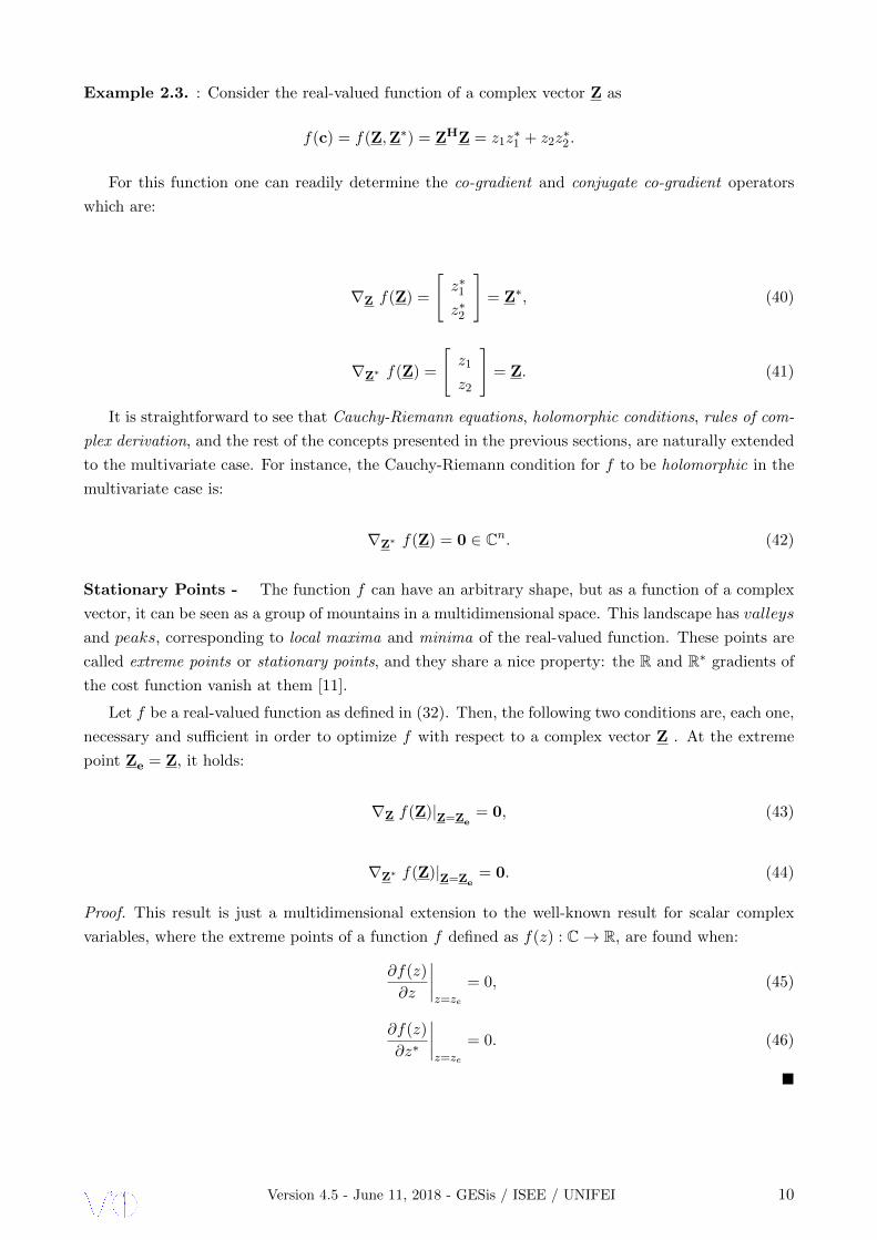
Example 2.3. : Consider the real-valued function of a complex vector Z as

f(c) = f(Z,Z∗) = ZHZ = z1z∗1 + z2z

∗2 .

For this function one can readily determine the co-gradient and conjugate co-gradient operators

which are:

∇Z f(Z) =

[z∗1z∗2

]= Z∗, (40)

∇Z∗ f(Z) =

[z1

z2

]= Z. (41)

It is straightforward to see that Cauchy-Riemann equations, holomorphic conditions, rules of com-

plex derivation, and the rest of the concepts presented in the previous sections, are naturally extended

to the multivariate case. For instance, the Cauchy-Riemann condition for f to be holomorphic in the

multivariate case is:

∇Z∗ f(Z) = 0 ∈ Cn. (42)

Stationary Points - The function f can have an arbitrary shape, but as a function of a complex

vector, it can be seen as a group of mountains in a multidimensional space. This landscape has valleys

and peaks, corresponding to local maxima and minima of the real-valued function. These points are

called extreme points or stationary points, and they share a nice property: the R and R∗ gradients of

the cost function vanish at them [11].

Let f be a real-valued function as defined in (32). Then, the following two conditions are, each one,

necessary and sufficient in order to optimize f with respect to a complex vector Z . At the extreme

point Ze = Z, it holds:

∇Z f(Z)|Z=Ze= 0, (43)

∇Z∗ f(Z)|Z=Ze= 0. (44)

Proof. This result is just a multidimensional extension to the well-known result for scalar complex

variables, where the extreme points of a function f defined as f(z) : C→ R, are found when:

∂f(z)

∂z

∣∣∣∣z=ze

= 0, (45)

∂f(z)

∂z∗

∣∣∣∣z=ze

= 0. (46)


Any algorithm that optimizes the cost function f should reach one of these extreme points, where

the criterion represented by the function is maximized, minimized, or reaches an inflexion point.

While one changes the vector Z, in fact it is changing the real value of the cost function f . For

each Z, the value of f is determined, but in general, the reverse does not always hold, so f is not an

injective function.

This means that one can move freely the vector in any direction, as one were walking on the

mountains, and watch for the effects on the objective function (that would be the height over the

multidimensional surface).

An interesting question is: which direction is the one that achieves the maximum rate of change?

If it is on the slopes of a valley, that direction leads us directly to the local minimum.

The Direction of Maximum Rate of Change - To answer that question, one looks at how a

small change on the vector variable is translated to the value of the cost function. The main result of

this section is stated in the following theorem:

Let f(Z) : Cn → R be a real-valued function of complex multivariate variable. Then, the direction

of maximum rate of change is given by

∇Z∗ f(Z) = 0. (47)

And thus, moving Z in the same direction of (47), the cost function f is maximized. On the other

hand, moving in the opposite direction, e.g., −∇Z∗ f(Z), the cost function f is minimized.

Proof. Using the differential rule (13) for vectors, yields to

df =(∇Z f(Z)

)TdZ +

(∇Z∗ f(Z)

)TdZ∗ ∈ R. (48)

Identifying the expression ∇X = 12(∇Z +∇Z∗) of the real part of a complex vector:

df = 2×Re(∇Z f(Z)

)TdZ. (49)

Using the multivariate equivalent of property (12) for real-valued functions, (49) becomes:

df=2×Re(∇Z∗ f(Z)

)HdZ

= 2×⟨∇Z∗ f(Z), dZ

⟩. (50)

This expression is proportional to the scalar product of two complex-valued vectors, ∇Z∗ f(Z) and dZ.

From basic geometry, one knows that the scalar product ( 〈·, ·〉 ) is maximized when the two vectors has

the same direction, and minimized when they have opposite directions. In general, one is interested

on minimizing the cost functions, because they usually represent an undesirable quality or an error of

the system.

Another interesting situation occurs when vectors ∇Z∗ f(Z) and dZ are orthogonal. The

scalar product of two orthogonal vector is null. One can interpret this fact as if the rate of change df

vanishes, so the cost function does not change. It is interesting to see that, obviously, the isobars of


the cost functions are defined by this situation. In fact, the locus of points orthogonal to the vector

∇Z∗ f(Z) locally define the points where the cost function f takes the same value. The following

example is a practical aid to better understand this issue.

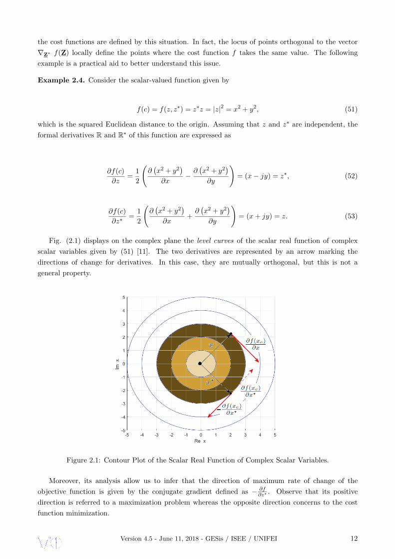
Example 2.4. Consider the scalar-valued function given by

f(c) = f(z, z∗) = z∗z = |z|2 = x2 + y2, (51)

which is the squared Euclidean distance to the origin. Assuming that z and z∗ are independent, the

formal derivatives R and R∗ of this function are expressed as

∂f(c)

∂z=

1

2

(∂(x2 + y2

)∂x

−∂(x2 + y2

)∂y

)= (x− jy) = z∗, (52)

∂f(c)

∂z∗=

1

2

(∂(x2 + y2

)∂x

+∂(x2 + y2

)∂y

)= (x+ jy) = z. (53)

Fig. (2.1) displays on the complex plane the level curves of the scalar real function of complex

scalar variables given by (51) [11]. The two derivatives are represented by an arrow marking the

directions of change for derivatives. In this case, they are mutually orthogonal, but this is not a

general property.

Figure 2.1: Contour Plot of the Scalar Real Function of Complex Scalar Variables.

Moreover, its analysis allow us to infer that the direction of maximum rate of change of the

objective function is given by the conjugate gradient defined as − ∂f∂z∗ . Observe that its positive

direction is referred to a maximization problem whereas the opposite direction concerns to the cost

function minimization.


Therefore, the vector

− ∂f

∂z∗, (54)

represents the direction of maximum descent, and the orthogonal direction represents the direction of

no local change.

Note that the same reasoning cannot be applied the gradient, i.e., ∂f∂z . Looking at (49), it is easy

to see that it does not represent an scalar product, so it does not gives any insight about the geometry

of the gradient of the cost function.

2.1.7 The Complex Jacobian Matrix

Let f(c) = f(z, z∗) ∈ Cm be a mapping

f := Cn → Cm

The generalization of (13) yields the vector form of differential rule3,

df(c) =∂f(c)

∂cdc =

∂f(c)

∂zdz +

∂f(c)

∂z∗dz∗ (55)

where the m×n matrix ∂f∂z is called the Jacobian, or Jacobian Matrix, of the mapping f , and the m×n

matrix ∂f∂z∗ the conjugate Jacobian of f . The Jacobian of f is often denoted by Jf and is computed

by applying the co-gradient operator component-wise to f ,

Jf (c) =∂f(c)

∂z=

∂f1(c)∂z...

∂fm(c)∂z

=

∂f1(c)∂z1

· · · ∂f1(c)∂zn

.... . .

...∂fm(c)∂z1

· · · ∂fm(c)∂zn

∈ Cm×n, (56)

and similarly the conjugate Jacobian, denoted by J∗f is computed by applying the conjugate co-gradient

operator component-wise to f ,

Jcf (c) =

∂f(c)

∂z∗=

∂f1(c)∂z∗

...∂fm(c)∂z∗

=

∂f1(c)∂z∗1

· · · ∂f1(c)∂z∗n

.... . .

...∂fm(c)∂z∗1

· · · ∂fm(c)∂z∗n

∈ Cm×n. (57)

With the above notation one can write the differential rule in (55) as

df(c) = Jf (c) dz + Jcf (c) dz∗. (58)

that when under the properties (11) and (12) component-wise to f , yields to the following identities:

∂f∗(c)

∂z∗=

(∂f(c)

∂z

)∗=(Jf (c)

)∗and

∂f∗(c)

∂z=

(∂f(c)

∂z∗

)∗=(Jcf (c)

)∗(59)

Note from (59) that,

(Jf (c)

)∗=

(∂f(c)

∂z

)∗=∂f∗(c)

∂z∗6= Jc

f (c) =∂f(c)

∂z∗. (60)

3At this point, the expression ∂f(c)∂c

dc only has meaning as a shorthand expression for ∂f∂z

dz + ∂f∂z∗ dz

∗, each term of

which must be interpreted formally as z and z∗ cannot be varied independently of each other.


Nonetheless, in the important special case that f(c) is real-valued (in which case f∗(c) = f(c)) one

have

f(c) ∈ Rm ⇒(Jf (c)

)∗=

(∂f(c))∗

∂z=∂f(c)

∂z∗= Jc

f (c). (61)

With (58), equation (61) yields to the following important fact which holds for real-valued functions

of complex variables f(c)4,

f(c) ∈ Rm ⇒ df(c) = Jf (c) dz +(Jf (c) dz

)∗= 2×Re

Jf (c) dz

= 2×Re

Jcf (c) dz∗

.

(62)

In other words, for holomorphic functions J∗ 6= Jc, whereas for real functions of complex variable,

i.e., non-holomorphic functions, the following equality holds: J∗ = Jc.

Finally, the complex derivatives showed above allow us to claim that they are often described by

more elegant expressions than their real counterparts.

2.2 Framework for CR− Calculus

2.2.1 Hermitian conjugate matrix

Also, the following definition will be required hereafter: Let z ∈ Cm; thenRz

∆= (Rez, Imz) ∈

R, Cz ∆= (z, z∗) ∈ C and

C∗z

∆= (z∗, z) =

Cz ∈ C. Furthermore the linear map

J∆=

[In j In

In −j In

](63)

which is a isomorphism from R to C and its inverse is given by J−1 = 12J

H , this latter defined as

Hermitian conjugate matrix. While In is the identity matrix of n order.

Example 2.5. : Taking into account the above definition, i.e.,

J =

[1 +j

1 −j

]→ J−1 = 1

2JH = 1

2(J∗)T = 12

([1 +j

1 −j

]∗)T=

= 12

(1 −j1 +j

)T= 1

2

[1 1

−j +j

]∴ JH =

[1 1

−j +j

]∆=

Hermitian

conjugate

matrix

2.2.2 SWAP operator

Additionally, it is advised to define a swap operator as

S∆=

[0 In

In 0

](64)

which is a isomorphism from C to the dual space C∗ which obeys the properties

S−1 = ST = S, (65)

4The real part of a vector (or matrix) is the vector (or matrix) of the real parts. Note that the mapping dz → df(c)

is not linear.


showing that S is symmetric and its own inverse, S2 = I.

In fact the swap operator is a block permutation matrix which permutes blocks of rows or blocks

of columns depending on whether S pre-multiplies or post-multiplies a matrix, respectively.

Example 2.6. : Now considering the operator defined above, i.e.,

S =

[0 1

1 0

]→ S−1 = ST = S =

[0 1

1 0

], for n = 1, and let a 2n × 2n matrix A be block

partitioned as

A =

(A11 A12

A21 A22

).

then pre-multiplication by S results in a block swap of the top n rows en masse with the bottom

n rows,

SA =

(A21 A22

A11 A12

).

Alternatively, post-multiplication by S results in a block swap of the first n columns with the last

n columns,

AS =

(A12 A11

A22 A21

).

It is also useful to note the result of a ”sandwiching” by S,

SAS =

(A22 A21

A12 A11

).

Additionally, it is straightforward to show that

I =1

2JT S J (66)

for J given by (63).

2.2.3 Mapping variables from R towards C domain

Now the linear map in (63) also defines one-to-one correspondence between the real gradient ∂

∂Rz

and complex gradient ∂

∂Cz, namely,

∂

∂Rz

= JT∂

∂Cz. (67)

Similarly, the real Hessian ∂2

∂Rz ∂

RzT can be transformed into several complex Hessian matrices, two

of which are

∂2

∂Rz ∂

RzT

=∂

∂Rz

(∂

∂Rz

)T= JT

∂

∂Cz

(∂

∂CzTJ

)= JT

∂2

∂Cz∂

CzTJ, (68)


∂2

∂Rz ∂

RzT

=∂

∂Rz

(∂

∂Rz

)T= JH

∂

∂Cz∗

(∂

∂CzTJ

)= JH

∂2

∂Cz∗∂

CzTJ. (69)

Notice that the complex Hessian matrix derived above is function of JT in (68) while of JH , i.e,

Hermitian conjugate matrix, in (69).

2.2.4 Mapping variables from C towards C domain

Consider a matrix M ∈ C2n×2n has the property that it is a linear mapping from C to C, such

that one can state

M ∈ (C,C) = M | Mc ∈ C,∀c ∈ C and M is linear ⊂ (C2n,C2n) = C2n×2n (70)

where (C,C) is a real vector space of linear operators, while (C2n,C2n) is a complex vector space of lin-

ear operators. Both are vector spaces over different fields, they cannot have a vector-subspace/vector-

parent-space relationship to each other. Note that (C,C) ⊂ (C2n,C2n) is just the statement that any

matrix which maps from C ⊂ C2n to C ⊂ C2n is also a linear mapping from C2n to C2n.

In order to determine the necessary and sufficient conditions for a matrix M ∈ C2n×2n to be an

element of (C,C) suppose that the vector c = col(z, z∗) ∈ C always maps to a vector s = col(ξ, ξ) ∈ Cunder the action of M , e.g., s = Mc. This relationship when expressed in block matrix is(

ξ

ξ

)=

[M11 M12

M21 M22

](z

z∗

). (71)

The first block row of this matrix equation yields the conditions

ξ = M11z +M12z∗,

while the complex conjugate of the second block row yields

ξ = M∗21z∗ +M∗22z,

and subtracting these two sets of equations results in the following condition on the block elements

of M ,

(M11 −M∗22) z − (M12 −M∗21)z∗ = 0.

With z = (x+ jy), the equality stated above can be spitted into two sets of conditions as

[(M11 −M∗22) + (M12 −M∗21)]x = 0

and

[(M11 −M∗22)− (M12 −M∗21)] y = 0.


Since these equations must hold for any x and y, they are equivalent to

(M11 −M∗22) + (M12 −M∗21) = 0

and

(M11 −M∗22)− (M12 −M∗21) = 0.

Therefore, adding and subtracting these two equations yields the necessary and sufficient condition

for M to be admissible (i.e., to act as a linear mapping from C to C),

M =

[M11 M12

M21 M22

]∈ C2n×2n is an element of (C,C) iff M11 = M∗22 and M12 = M∗21. (72)

The necessary and sufficient admissibility condition (72) is better expressed in the following equiv-

alent form

M ∈ (C,C)⇐⇒M = SM∗S ⇔M = SMS (73)

which is straightforward to verify.

Given an arbitrary matrix M ∈ C2n×2n, we can define a natural mapping of M into (C,C) ⊂C2n×2n by

P (M)∆=M + SM∗S

2∈ (C,C), (74)

in which case the admissibility condition (73) has an equivalent restatement as

M ∈ (C,C)⇔ P (M) = M. (75)

Finally, it is also straightforward to demonstrate that

∀M ∈ C2n×2n, P (P (M)) = P (M). (76)

I.e., P is an idempotent mapping of C2n×2n onto (C,C), P 2 = P .

2.3 Partial Conclusions

In this section the Wirtinger derivatives is derived and it is showed how easy becomes up to now

to operate any application in conjugate coordinates. It is shown that holomorfic functions are in fact

a subset of functions of complex variables that does not depend upon their corresponding complex

conjugate variables. Consequently, the Wirtinger derivatives is a general operator that allows us to

expand any nonlinear function in Taylor’s serie, i.e., whichever they are holomorfic or non-holomorfic,

aiming the derivation of classical algorithms usually applied to power systems problems, as Newtow-

Raphson and Gauss-Newton, to cite a few.


3 Complex-Valued Power Flow Analysis (CV-PFA)

Numerical solutions for solving power system application are typically carried out in the real

domain. Examples are power flow analysis and power system state estimation, among others. It turns

out that these solutions are not well suited for modeling voltage and current phasor, which were intro-

duced by Steinmetz [1,12]. To circumvent this difficulty, iterative and non-iterative algorithms carried

out in the complex domain were proposed recently in the literature; applications in power transmission

and distributions systems are described in [13], [14], [15] for iterative methods and [16], [17] [18] for

non-iterative methods. Iterative complex-valued power flow calculation is addressed by Wang [16] by

using the Wirtinger calculus [3], [2]. On the other hand, [15] makes use of the method proposed by

Brandwood [19]. However, both approach does not use any Wirtinger derivatives. Instead, they use

nodal network equations to derive a first- or second-order Newton-Raphson algorithm. Furthermore,

in order to add numerical robustness, a fourth-order Levenberg-Marquardt algorithm is employed to

the CV PFA approach because of its nice bi-quadratic convergence property, instead of the well-known

quadratic convergence property of the classical Newton-Raphson. Recall that this algorithm is prone

to colapse when the power system network is ill-conditioned, i.e., it is heavily loaded or presents

branches with high R/X ratio.

In this section is presented the derivation of a complex-valued power flow (CV-PFA) derived

straightforwardly from Wirtinger’s Work [3], in contrast to the approach brought by [13], [14]. Firstly,

the whole power flow modeling starts based on the classical nodal equation as presented in [20]. In

the second approach the analytical model is derived through the general power flow equations. The

main reason for this latter option is the transformer model with tap position off-nominal, including

phase-shifters [21], [22]. Further discussions on this issue are addressed throughout the derivation of

the approaches.

3.1 Nodal Equation

This approach requires the Nodal Admittance matrix buiding, e.g.,

I = Ybus V , (77)

thus the complex nodal power can be expressed as

S = diag(V ) I∗, (78)

or

S = diag(V ) Y∗bus V∗. (79)

Then, the nodal complex power at bus− k, i.e., Sk, is

Sk = Vk Y∗kk V

∗k + Vk

N∑m=0m 6=k

Y ∗km V ∗m, (80)

where N + 1 is the number of network nodes, and the node 0 is assigned as the slack node.


3.2 Complex-Valued Power Flow Equations

The complex-valued power flow equations that model any type of branch in an electrical network,

i.e., transmission lines and phase- and phase-shifting-transformers are as follows:

Skm = Vk

(y∗km

akma∗km

− j bshkm)V ∗k − Vk

y∗kmakm

V ∗m, (81)

Smk = Vm

(y∗km − j bshkm

)V ∗m − Vm

y∗kma∗km

V ∗k . (82)

and

S∗km = V ∗k

(ykm

a∗kmakm+ j bshkm

)Vk − V ∗k

ykma∗km

Vm, (83)

S∗mk = V ∗m

(ykm + j bshkm

)Vm − V ∗m

ykmakm

Vk. (84)

In the set of equations (81-84), the general off-nominal tap transformer model is composed by an

ideal transformer with complex turns ratio aejφ : 1 in series with its admittance or impedance [21].

3.3 Wirtinger Derivatives Applied to the Power Flow Equations

Firstly, let us assume that the complex power injections, Sk and Sm, are equal to the power flows Skm

and Smk, respectively. Then, applying the Wirtinger calculus to the complex power flow equation

given by (81) yields

∂Sk∂Vk

∣∣∣∣V ∗k =Const

=

(y∗km

akma∗km

− j bshkm)V ∗k −

y∗kmakm

V ∗m, (85)

∂Sk∂V ∗k

∣∣∣∣Vk=Const

= Vk

(y∗km

akma∗km

− j bshkm), (86)

∂Sk∂Vm

∣∣∣∣V ∗m=Const

= 0.0, (87)

∂Sk∂V ∗m

∣∣∣∣Vm=Const

=− Vky∗kmakm

, (88)

∂Sk∂akm

∣∣∣∣a∗km=Const

=− Vk(

y∗kma2kma

∗km

)V ∗k + Vk

y∗kma2km

V ∗m, (89)

∂Sk∂a∗km

∣∣∣∣akm=Const

=− Vk(

y∗kmakm(a∗km)2

)V ∗k . (90)


and given by (82) yields

∂Sm∂Vm


=(y∗km − j bshkm

)V ∗m −

y∗kma∗km

V ∗k , (91)

∂Sm∂V ∗m


= Vm

(y∗km − j bshkm

), (92)

∂Sm∂Vk


= 0.0, (93)

∂Sm∂V ∗k


=− Vmy∗kma∗km

, (94)

∂Sm∂akm


= 0.0, (95)

∂Sm∂a∗km


= Vmy∗km

(a∗km)2V ∗k . (96)

and given by (83) yields

∂S∗k∂Vk


= V ∗k

(ykm

a∗kmakm+ j bshkm

), (97)

∂S∗k∂V ∗k


=

(ykm

a∗kmakm+ j bshkm

)Vk −

ykma∗km

Vm, (98)

∂S∗k∂Vm


=− V ∗kykma∗km

, (99)

∂S∗k∂V ∗m


= 0.0, (100)

∂S∗k∂akm


=− V ∗k(

ykma∗kma

2km

)Vk, (101)

∂S∗k∂a∗km


=− V ∗k(

ykm(a∗km)2akm

)Vk + V ∗k

ykm(a∗km)2

Vm. (102)

Finally, applying Wirtinger calculus to (84) yields

∂S∗m∂Vk


=− V ∗mykmakm

, (103)

∂S∗m∂V ∗k


= 0.0, (104)

∂S∗m∂Vm


=V ∗m

(ykm + j bshkm

), (105)

∂S∗m∂V ∗m


=(ykm + j bshkm

)Vm −

ykmakm

Vk, (106)

∂S∗m∂akm


= V ∗mykma2km

Vk, (107)

∂S∗m∂a∗km


= 0.0. (108)


3.4 Bus Models in the Complex Domain

3.4.1 Slack-Bus Type

The complex voltage at a slack-bus type is known, once the magnitude and phase-angle values

are specified for the reference bus.

3.4.2 PQ-Bus Type

With the active- and reactive-power demand specified for a PQ node, the following complex

mismatches functions are expressed as

Mk = Sk − (Pks + j Qks), (109)

M∗k = S∗k − (Pks − j Qks), (110)

where Pks and Qks, are the specified active- and reactive-power injection at node k, respectively.

In order to derive the Newton-Raphson algorithm in the complex domain, the Jacobian matrix

elements in complex form corresponding to each PQ−Bus are formed based on the Wirtinger deriva-

tives of Mk and M∗k with respect to the complex and the complex conjugate nodal voltage magnitudes,

yielding

∂Mk

∂Vk


=N∑

m∈Ωi

∂Sk∂Vk


, (111)

∂Mk

∂V ∗k


=N∑

m∈Ωi

∂Sk∂V ∗k


, (112)

∂Mk

∂Vm


= 0.0, (113)

∂Mk

∂V ∗m


=N∑

m∈Ωi

∂Sk∂V ∗m


, (114)

and

∂M∗k∂Vk


=

N∑m∈Ωi

∂S∗k∂Vk


, (115)

∂M∗k∂V ∗k


=

N∑m∈Ωi

∂S∗k∂V ∗k


, (116)

∂M∗k∂Vm


=

N∑m∈Ωi

∂S∗k∂Vm


, (117)

∂M∗k∂V ∗m


= 0.0. (118)

Here Ωi in (111-118) is the set of neighboring buses connected to the kth − bus and N is the total

number of buses. Moreover, in (113-114) and (117-118), m 6= 0 and m 6= k. We highlight that the

right hand side (rhs) of (116) is the nodal complex current at node k while the rhs of (111) is the

complex conjugate of the nodal current at node k.


3.4.3 PV-Bus Type

As the active-power generation and the terminal voltage magnitude at a PV − bus are both

specified, i.e., Pks and Vks, respectively, the sum of Mk in (109) and M∗k in (110) gives the complex

residual function, Mkg, which is related to the active-power constraint as follows:

Mkg = Mk +M∗k ,

= Sk + S∗k − 2× Pks.(119)

The second complex residual function Ekg for a generator node k is formed, using the voltage magni-

tude constraint given by

|Ekg| = |Vk|2 − |Vks|2 , (120)

where the |Vks| is the specified voltage magnitude at Node k.

As |Vk|2 = Vk V∗k , (120) can be expressed in the complex domain as

Ekg = Vk V∗k − |Vks|

2 , (121)

and the Jacobian matrix elements associated with a Generator node k are obtained by taking the

partial derivatives of the complex residual functions in (119) and (121) with respect to Vk and V ∗k ,

yielding

∂Mkg

∂Vk


=∂Mk

∂Vk


+∂M∗k∂Vk


, (122)

∂Mkg

∂V ∗k


=∂Mk

∂V ∗k


+∂M∗k∂V ∗k


, (123)

∂Mkg

∂Vm


=∂Mk

∂Vm


+∂M∗k∂Vm


, (124)

∂Mkg

∂V ∗m


=∂Mk

∂V ∗m


+∂M∗k∂V ∗m


, (125)

where in (124-125), m 6= 0 and m 6= k. Moreover, note that the rhs of (122-125) are defined in

(111-118). On the other hand, the partial derivatives of Ekg in (121) with respect to Vk and V ∗k are

expressed as

∂Ekg∂Vk


= V ∗k , (126)

∂Ekg∂V ∗k


= Vk, (127)

and the partial derivaives with respect to Vm and V ∗m are given by

∂Ekg∂Vm


= 0.0, for m 6= 0 and m 6= k, (128)

∂Ekg∂V ∗m


= 0.0, for m 6= 0 and m 6= k, (129)


3.4.4 PQV-Bus Type

This type of bus is referred to model On-Load-Tap-Changer (OLTC ), which can be a phase-

transformer for local and nearby bus voltage regulation or a phase-shifting-transformer for controlling

the active power flow transmitted over a line [23]. It is also suited to model a DC link of a voltage-

sourced converter [24], [25]. As the active- and reactive-power demand are specified, the complex

mismatches functions as stated in (109) and (110) are employed. Nonetheless, it is worth to recall

that the OLTC tap position allows us to regulate the voltage magnitude at either k− or m−bus. Let

us assume that the m−bus voltage is regulated, leading to the following mismatches functions:

Mm = akm − a∗km − 2×=akm, (130)

Em = Vm V ∗m − |Vms |2 , (131)

Here =akm is the specified imaginary part of the complex tap value, e.g, for a phase-transformer,

we have =akm = 0.0; otherwise, it is a phase-shifter-transformer and instead of (130), (119) is used.

In (131), Vms is the specified voltage at node m, i.e., the regulated nodal voltage, yielding the partial

derivatives of (130) and (131) given by

∂Mm

∂akm


= 1.0, (132)

∂Mm

∂a∗km


= −1.0, (133)

and

∂Em∂Vm


= V ∗m, (134)

∂Em∂V ∗m


= Vm. (135)

When (119) is used, the corresponding partial derivatives are those defined in (89-90) and (101-

102).

3.5 Complex-Valued Iterative Solution

3.5.1 The Newton-Raphson Algorithm

When the slack bus is excluded, the state variables vector in the complex conjugate coordinate

becomes

xc = [V1, V2, . . . , VN−1, V∗

1 , V∗

2 , . . . , V∗N−1]T , (136)

and the mismatches vector reduces to

M (xc) = [M1,M2, . . . ,MN−1,M∗1 ,M

∗2 , . . . ,M

∗N−1]T . (137)

If Node k (for k = 1, 2, . . . , N −1) is a PV − bus or a PQV − bus, the pair of elements Mk and M∗kin (137) are replaced by Mkg and Ekg as in (119) and (121) or replaced by Mm and Em as in (130)

and (131), respectively. Here, the objective is to calculate xc that satisfies

M (xc) = 0. (138)


It follows that the linearization of (138) from one step to the sequel is given by

M(xc

(ν−1))

+ J(xc(ν−1)) ∆x(ν)

c = 0, (139)

and

xc(ν) = xc

(ν−1) −[J(ν−1)

]−1M(xc

(ν−1)), (140)

or

∆x(ν)c = −

[J(ν−1)

]−1M(xc

(ν−1)), (141)

where J is the complex-valued Jacobian matrix in the complex conjugate coordinate. So, the update

equation is given by

xc(ν) = xc

(ν−1) + ∆x(ν)c . (142)

The convergence criterion can be the same that is often assumed in the R− domain, i.e.,

∥∥∥∆x(ν)c

∥∥∥∞≤ tol (≈ 10−3). (143)

where ‖·‖∞ is defined as the infinity norm and ν is the iteration counter. In the complex domain, the

convergence criterion is chosen to be the infinity norm of the ∆x(ν)c of the complex conjugate partition

as explained next.

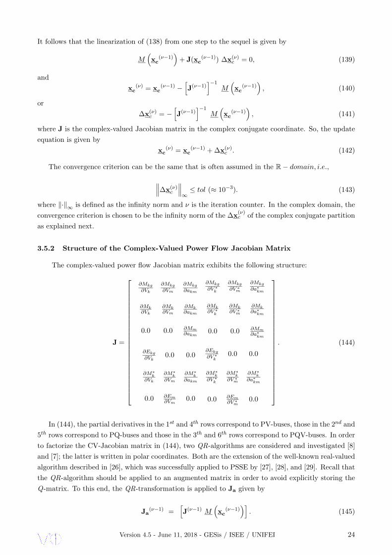
3.5.2 Structure of the Complex-Valued Power Flow Jacobian Matrix

The complex-valued power flow Jacobian matrix exhibits the following structure:

J =

∂Mkg

∂Vk

∂Mkg

∂Vm

∂Mkg

∂akm

∂Mk∂Vk

∂Mk∂Vm

∂Mk∂akm

0.0 0.0 ∂Mm∂akm

∂Mkg

∂V ∗k

∂Mkg

∂V ∗m

∂Mkg

∂a∗km

∂Mk∂V ∗k

∂Mk∂V ∗m

∂Mk∂a∗km

0.0 0.0 ∂Mm∂a∗km

∂Ekg

∂Vk0.0 0.0

∂M∗k∂Vk

∂M∗k∂Vm

∂M∗k∂akm

0.0 ∂Em∂Vm

0.0

∂Ekg

∂V ∗k0.0 0.0

∂M∗k∂V ∗k

∂M∗k∂V ∗m

∂M∗k∂a∗km

0.0 ∂Em∂V ∗m

0.0

. (144)

In (144), the partial derivatives in the 1st and 4th rows correspond to PV-buses, those in the 2nd and

5th rows correspond to PQ-buses and those in the 3th and 6th rows correspond to PQV-buses. In order

to factorize the CV-Jacobian matrix in (144), two QR-algorithms are considered and investigated [8]

and [7]; the latter is written in polar coordinates. Both are the extension of the well-known real-valued

algorithm described in [26], which was successfully applied to PSSE by [27], [28], and [29]. Recall that

the QR-algorithm should be applied to an augmented matrix in order to avoid explicitly storing the

Q-matrix. To this end, the QR-transformation is applied to Ja given by

Ja(ν−1) =

[J(ν−1) M

(xc

(ν−1))]. (145)


On the other hand, it turns out that if we store the sequence of rotations in compact form, the

complex-valued Jacobian matrix can be kept constant, implying that only the right-hand-side vector

is updated throughout the final iterations. Here, the solution of (141) is reached by performing a

simple back-substitution over the factorization of (145), yielding

J(ν−1)a =

[Tc Mc

]. (146)

where Tc is an upper triangular matrix of dimension-2n × 2n, and Mc comprises the corresponding

rows in the updated rhs vector, dimension− 2n × 1, for n = N − 1. Then, (141) can be expressed

through

∆x(ν)c = Tc Mc. (147)

Note that when executing the algorithm given by (147), only the complex conjugate state vector,

x∗, has to be updated. Therefore, the steps defined in (141) and (143) can be numerically decoupled,

suggesting that only the Jacobian matrix associated with x∗ has to be stored and factorized.

3.5.3 The Fourth-Order Levenberg-Marquardt as Applied to CV-PFA

In the state-of-the-art of numerical analysis, many proposals can be found aiming to solve ill-

conditioned nonlinear system of equations as [30], [31], [32], [33], [34] to cite a few. In power systems

analysis, Brown’s and Brent’s methods have been applied to solve ill-conditioned systems [35], [36],

[37], [38], [39] and [40]. Nonetheless, in [41] the researchers have employed Yang’s proposal [42] which

is based on the Levenberg-Marquardt algorithm that is usually derived for optmization problem [6].

After tireless checking of the numerical robustness stated in [42], [43], [44] and [45] by using the

nonlinear systems of equations in real domain, as Rosenbrok’s; Brown’s 1 and 2; Brown-Conte and

Powell’s test functions extracted from [34], the algorithm proposed by Yang [42] and Fan [43] have

presented best performance and easy encoding task. In this work the Yang’s proposal is presented

as applied to CV-PFA. Nonetheless, as the goal is to enhance the numerical robustness, the Barel’s

format equation [6] is assumed once it is based on the Jacobian instead of the Gain matrix as stated

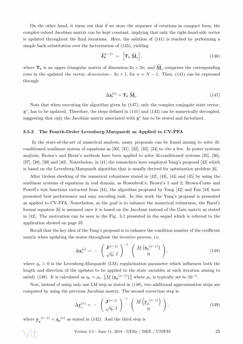
in [42]. The motivation can be seen in the Fig. 3.1 presented in the sequel which is referred to the

application showed on page 35.

Recall that the key idea of the Yang’s proposal is to enhance the condition number of the coefficent

matrix when updating the states throughout the iterative process, i.e.

∆x(ν)c = −

(J(ν−1)

√ην I

)−1 (M(xc

(ν−1))

0

), (148)

where ην > 0 is the Levenberg-Marquardt (LM) regularization parameter which influences both the

length and direction of the updates to be applied to the state variables at each iteration aiming to

satisfy (138). It is calculated as ην = µν∥∥M (

xc(ν−1)

)∥∥ where µν is typically set to 10−5.

Now, instead of using only one LM step as stated in (148), two additional approximation steps are

computed by using the previous Jacobian matrix. The second correction step is

∆y(ν)c

= −

(J(ν−1)

√ην I

)−1 (M(y

c(ν−1)

)0

), (149)

where yc

(ν−1) = xc(ν) as stated in (142). And the third step is


Figure 3.1: IEEE-11 Bus: Condition Number.

∆z(ν)c = −

(J(ν−1)

√ην I

)−1 (M(zc

(ν−1))

0

), (150)

where zc(ν−1) = y

c(ν) = y

c(ν−1) + ∆z

(ν)c . Thus, the convergence checking should be carried out over

this last approximation step, yielding

∥∥∥∆z(ν)c

∥∥∥∞≤ tol (≈ 10−3). (151)

If (151) is satisfied, stop and print out the results. Otherwise, calculate the ratio of error deduction

errν = Aredν/Predν , where

Aredν =∥∥∥M (

xc(ν−1)

)∥∥∥2−∥∥∥M(xc

(ν−1) + ∆xc(ν) + ∆y

c(ν) + ∆zc

(ν))∥∥∥2, (152)

Predν =∥∥M (

xc(ν−1)

)∥∥2 −∥∥∥M (

xc(ν−1)

)+ J(ν−1) ∆x

(ν)c

∥∥∥2+

∥∥∥M (y

c(ν−1)

)∥∥∥2−∥∥∥M (

yc

(ν−1))

+ J(ν−1) ∆y(ν)c

∥∥∥2+

∥∥M (zc

(ν−1))∥∥2 −

∥∥∥M (zc

(ν−1))

+ J(ν−1) ∆z(ν)c

∥∥∥2.

(153)

The state vector is updated through

xc(ν) =

xc

(ν−1) + ∆x(ν)c + ∆y(ν)

c+ ∆z(ν)

c , if errν > p0

xc(ν−1), otherwise.

(154)


where p0 is a parameter that is chosen between 0 and 1. Finally the LM regularization parameter ην

is updated as

ην =

4 ην if errν < p1

ην if errν ∈ [p1, p2]

maxην

4, λ

if errν > p2

(155)

where 0 < p0 ≤ p1 ≤ p2 < 1 and ην > λ > 0. Now the iteration counter is update, i.e., ν = ν + 1 and

it is checked if the maximum iteration number is reached; if that is the case, terminate the algorithm

and print out the results, otherwise starts the whole process going back to equation (148).

Remark that Jacobian matrix J is evaluated only once at the ν−th iteration, which is an appealing

property for the biquadratic convergence rate of the proposed approach. The latter can be proved

easily using the same theorems shown in [42]. Note that the calculation of the Jacobian matrix is

time consuming for large-scale systems. Thanks to the biquadratic convergence rate of the proposed

approach, the number of iterations is reduced significantly. On the other hand, the linerization error

of the nonlinear equation is compensated through the two additional approximate LM steps. This im-

proves the numerical robustness of the proposed approach remarkably under highly stressed operating

conditions.

Finally, note that there are several parameters that should be set before the iterative LM-based

CV-PFA has started. Among them, the initial value of µ, the p0, p1, p2 and λ. The initial value of

µ, which is usually set to 10−5, has little impact on the iterative process once it is either updated,

whereas for p0, p1, p2 and λ, we set them as p0 = 10−4, p1 = 0.25, p2 = 0.75 and λ = 0.65 following the

recommendation stated in [42]. We find that this set of values works well for different test systems.

3.6 Numerical Results

3.6.1 Small Example: CV-Power Flow Analysis

In the sequel the CV Power Flow modeling is applied to a small example system which

diagram is showed in Fig. 3.2, while the corresponding branch parameters and bus data, both in pu

(Vbase= 230 kV ; Sbase= 100 MVA), are presented in Table 3.1 and 3.2, respectively.

Figure 3.2: Small 3-Bus System.


Table 3.1: Branches Data.

Branch Serie Shunt

i→ jR X Charging Y/2

pu pu MVAr pu

1-2 0.0012 0.0021 39.2 0.196

1-3 0.0150 0.0400

2-3 0.3000 1.6000

Table 3.2: Bus Data.

Bus Specified Quantities in pu

Type Pg V Pload Qload

PV-2 1.0000 1.0000 0.2160 0.0918

PQ-3 2.700 1.620

The nodal admittance matrix, i.e., Ybus, yields to

Ybus =

213.3474 −j 380.8922 −205.1282 +j 358.9744 −8.2192 +j 21.9178

−205.1282 +j 358.9744 205.2414 −j 359.3821 −0.1132 +j 0.6037

−8.2192 +j 21.9178 −0.1132 +j 0.6037 8.3324 −j 22.3256

The whole set of intermediary results throughout the iterative process is presented in the sequence.

As in the real-domain, the elements of the complex-valued Jacobian matrix remain practically

unchanged after the second iteration, which suggest that we may keep them constant thereafter.

Moreover, the computation of some entries can be avoided because they are complex conjugates of

other variables; it turns out that these elements are PV-nodes.

J (ν=0) =

413.6193× e−j 60.268 0.4232× e−j 74.484 413.6193× e+j 60.268 0.4232× e+j 74.484

0.1960× e+j 90.000 0.6143× e−j 100.619 23.8298× e+j 69.533

1.0000× ej 0.000 1.0000× ej 0.000

0.6143× e+j 100.619 23.8298× e−j 69.533 0.1960× e+j 90.000

J (ν=1) =

414.4312× e−j 60.323 0.4232× e−j 74.616 414.4312× e+j 60.323 0.3842× e+j 69.158

3.1443× e−j 148.587 0.5577× e−j 105.946 21.6334× e+j 64.207

1.0000× e−j 0.132 1.0000× e+j 0.132

0.5577× e+j 105.946 23.8298× e−j 69.665 3.1443× e+j 148.587

J (ν=2) =

414.3163× e−j 60.313 0.4232× e−j 74.599 414.3180× e+j 60.313 0.3765× e+j 68.935

3.5321× e−j 143.603 0.5465× e−j 106.168 21.2006× e+j 63.984

1.0000× e−j 0.115 1.0000× e+j 0.115

0.5452× e+j 106.041 23.8298× e−j 69.648 3.5232× e+j 144.712


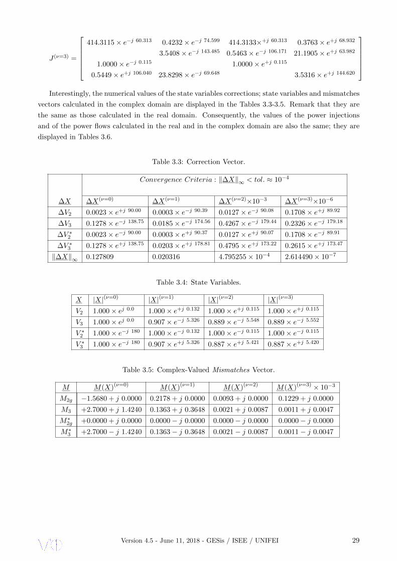
J (ν=3) =

414.3115× e−j 60.313 0.4232× e−j 74.599 414.3133×+j 60.313 0.3763× e+j 68.932

3.5408× e−j 143.485 0.5463× e−j 106.171 21.1905× e+j 63.982

1.0000× e−j 0.115 1.0000× e+j 0.115

0.5449× e+j 106.040 23.8298× e−j 69.648 3.5316× e+j 144.620

Interestingly, the numerical values of the state variables corrections; state variables and mismatches

vectors calculated in the complex domain are displayed in the Tables 3.3-3.5. Remark that they are

the same as those calculated in the real domain. Consequently, the values of the power injections

and of the power flows calculated in the real and in the complex domain are also the same; they are

displayed in Tables 3.6.

Table 3.3: Correction Vector.

Convergence Criteria : ‖∆X‖∞ < tol. ≈ 10−4

∆X ∆X(ν=0) ∆X(ν=1) ∆X(ν=2)×10−3 ∆X(ν=3)×10−6

∆V2 0.0023× e+j 90.00 0.0003× e−j 90.39 0.0127× e−j 90.08 0.1708× e+j 89.92

∆V3 0.1278× e−j 138.75 0.0185× e−j 174.56 0.4267× e−j 179.44 0.2326× e−j 179.18

∆V ∗2 0.0023× e−j 90.00 0.0003× e+j 90.37 0.0127× e+j 90.07 0.1708× e−j 89.91

∆V ∗3 0.1278× e+j 138.75 0.0203× e+j 178.81 0.4795× e+j 173.22 0.2615× e+j 173.47

‖∆X‖∞ 0.127809 0.020316 4.795255× 10−4 2.614490× 10−7

Table 3.4: State Variables.

X |X|(ν=0) |X|(ν=1) |X|(ν=2) |X|(ν=3)

V2 1.000× ej 0.0 1.000× e+j 0.132 1.000× e+j 0.115 1.000× e+j 0.115

V3 1.000× ej 0.0 0.907× e−j 5.326 0.889× e−j 5.548 0.889× e−j 5.552

V ∗2 1.000× e−j 180 1.000× e−j 0.132 1.000× e−j 0.115 1.000× e−j 0.115

V ∗3 1.000× e−j 180 0.907× e+j 5.326 0.887× e+j 5.421 0.887× e+j 5.420

Table 3.5: Complex-Valued Mismatches Vector.

M M(X)(ν=0) M(X)(ν=1) M(X)(ν=2) M(X)(ν=3) × 10−3

M2g −1.5680 + j 0.0000 0.2178 + j 0.0000 0.0093 + j 0.0000 0.1229 + j 0.0000

M3 +2.7000 + j 1.4240 0.1363 + j 0.3648 0.0021 + j 0.0087 0.0011 + j 0.0047

M∗2g +0.0000 + j 0.0000 0.0000− j 0.0000 0.0000− j 0.0000 0.0000− j 0.0000

M∗3 +2.7000− j 1.4240 0.1363− j 0.3648 0.0021− j 0.0087 0.0011− j 0.0047


Table 3.6: CV-Power Flow Report.

Coordinates

Sk Retanguar Polar

(Pk ± j Qk) |Sk| × e±j ϕ

S1 +2.0788 + j 2.2844 3.0887× e+j 47.697

S2 +0.7841− j 0.5449 0.9548× e−j 34.802

S3 −2.6999− j 1.6199 3.1487× e−j 149.036

Skm (Pkm ± j Qkm) |Skm| × e±j θkm

S12 −0.7183 + j 0.4114 0.8277× e+j 150.199

S21 +0.7192− j 0.4099 0.8277× e−j 29.686

S13 +2.7972 + j 1.8730 3.3663× e+j 33.806

S31 −2.6368− j 1.4171 2.9935× e−j 151.745

S23 +0.0649− j 0.1350 0.1498× e−j 64.323

S32 −0.0631− j 0.2028 0.2124× e−j 107.289

3.6.2 IEEE Test Systems: well-conditioned systems

Table 3.7 provides the parameters of the IEEE test power systems while Figs. 3.3-3.6 display the

sparsity structures of the Jacobian matrices in the the C-domain given by (144) as compared to those

derived in the R-domain.

Table 3.7: Features of the IEEE Test systems

IEEE-Test Bus Systems -14 -30 -57 -118

No. of PV-bus (NPV ) 4 5 6 53

No. of PQ-bus (NPQ) 9 24 50 64

No. of transformers 3 4 15 9

No. of transmission lines + shunt 21 43 83 200

R-Valued: n = (NPV + 2×NPQ) 22 53 106 181

C-Valued: 2n = 2× (NPV +NPQ) 26 58 112 234


(a) (b)

Figure 3.3: Sparsity structure of (a) real-valued Jacobian matrix; (b) complex-valued Jacobian matrix

of the IEEE 14-bus system.

(a) (b)



(a) (b)




(a) (b)



Clearly, the diagonal blocks in the complex Jacobian matrix are practically diagonal matrices,

which prompt its factorization. On the other hand, Table 3.8 provides the number of iterations,

the condition number and the non-zero counts associated with the real-valued and complex-valued

Jacobian matrices.

Table 3.8: Sparsity and Numerical Analysis

IEEE-Test Systems -14 -30 -57 -118

No. of iterations:

X RV-NR power flow 4 4 4 4

X CV-NR/LM power flow 4/2 4/2 5/2 4/2

Condition Number:

X RV-Jacobian matrix 117.8 473.3 826.1 3166.9

X CV-Jacobian matrix 118.0 487.5 815.8 3276.8

X RV/CV Ratio 0.99 0.97 1.01 0.97

Nonzero counts:

X RV-Jacobian matrix 144 375 718 1051

X CV-Jacobian matrix 124 272 520 1160

X RV/CV Ratio 1.16 1.38 1.38 0.90

Table 3.8 allows us to infer that the complex-valued power flow algorithm has numerical perfor-

mance and sparsity structure very similar to the real-valued counterpart; specifically, it requires the

same number of iterations to reach the solution (tol. ∼ 10−4) and it exhibits the same numerical

robustness and sparsity structure. Furthermore, as the fourth-order Levenberg-Marquadt algorithm

based on power flow analysis, CV-LMPFA for short, is now available in complex domain; notice that

it requires just 2 (two) iterations to reach the convergence in all of the well-conditioned IEEE test

systems.

Figs. 3.7 to 3.10 display the profiles of the voltage and phase angle at each bus of the IEEE 14-,

30-, 57-, and 118-bus systems. Remark that the results produced by the real- and complex-valued

Newton-Raphson power flow analysis are completely overlaid. Furthermore, in Table 3.9 is presented

the relative maximum bias between the corresponding state variables calculated in the complex and


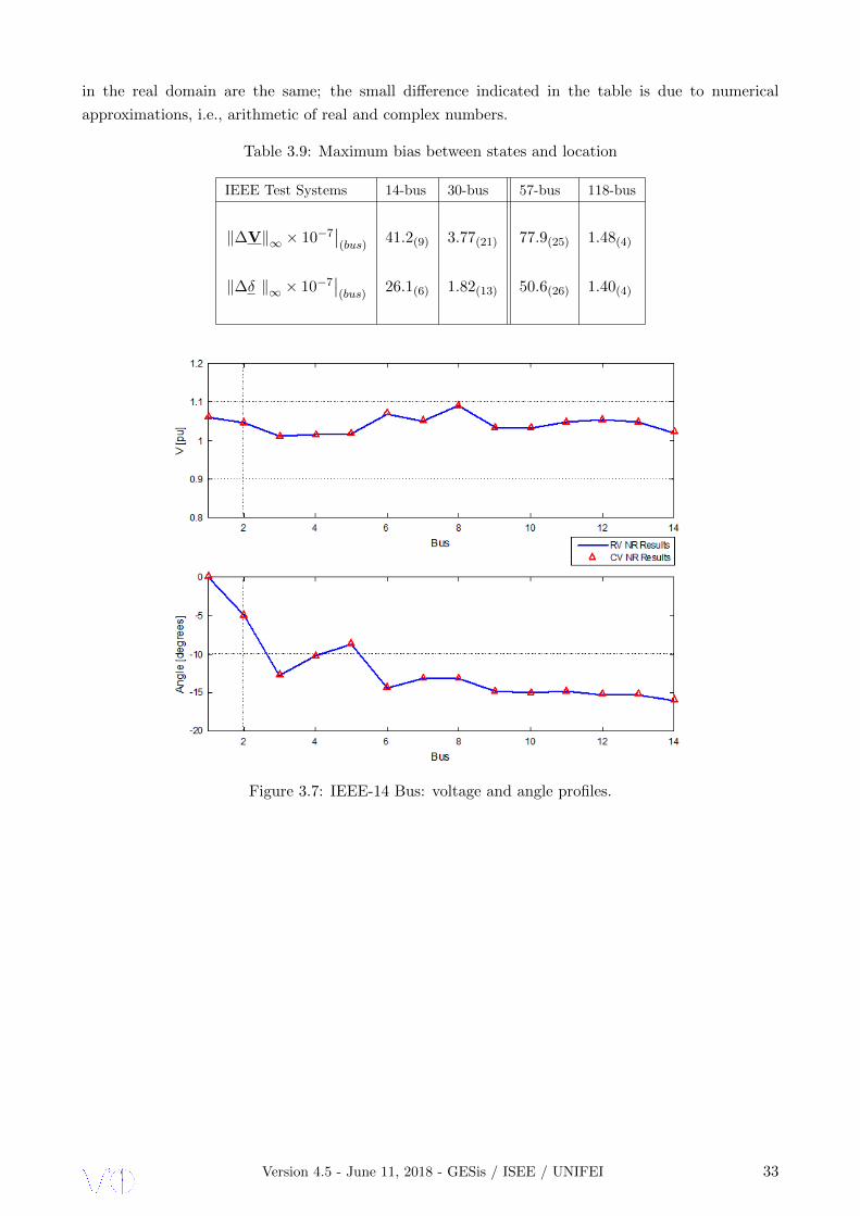
in the real domain are the same; the small difference indicated in the table is due to numerical

approximations, i.e., arithmetic of real and complex numbers.

Table 3.9: Maximum bias between states and location

IEEE Test Systems 14-bus 30-bus 57-bus 118-bus

‖∆V‖∞ × 10−7∣∣(bus)

41.2(9) 3.77(21) 77.9(25) 1.48(4)

‖∆δ ‖∞ × 10−7∣∣(bus)

26.1(6) 1.82(13) 50.6(26) 1.40(4)

Figure 3.7: IEEE-14 Bus: voltage and angle profiles.






3.6.3 IEEE Test Systems: ill-conditioned systems

The simulations carried out on the well-known ill-conditioned IEEE 11-Bus system are presented

in the sequence. The main features of this systems are its heavily loaded condition and radial topology.

The complex-valued Levenberg-Marquardt approach (CV-LMPFA) got successful performance in all

cases while the complex-valued Newton-Raphson algorithm (CV-NRPFA) has collapsed. The one

line diagram for the 11-Bus system is depicted in Fig. 3.11.

Figure 3.11: IEEE-11 Bus: one line diagram.

The power flow network data for the ill-conditioned 11-Bus system are presented in Tables 3.10

and 3.11.


Table 3.10: ill-conditioned IEEE-11 Bus Data.

Bus V δ Load Generator

No. code pu degree MW MVAr Mw MVAr Qmin Qmax

1 1 1.024 0.0 0.0 0.0 0.0 0.0 0 0

2 2 1.000 0.0 0.0 0.0 0.0 0.0 -1 +1

3 0 1.000 0.0 12.8 6.2 0.0 0.0 0 0

4 2 1.000 0.0 0.0 0.0 0.0 0.0 -1 +1

5 0 1.000 0.0 16.5 8.0 0.0 0.0 0 0

6 0 1.000 0.0 9.0 6.8 0.0 0.0 0 0

7 2 1.000 0.0 0.0 0.0 0.0 0.0 -1 +1

8 2 1.000 0.0 0.0 0.0 0.0 0.0 -1 +1

9 0 1.000 0.0 2.6 0.9 0.0 0.0 0 0

10 2 1.000 0.0 0.0 0.0 0.0 0.0 -1 +1

11 0 1.000 0.0 15.8 5.7 0.0 0.0 0 0

Table 3.11: ill-conditioned IEEE-11 Bus Branches Data.

Branches Impedance Half Susceptance Transformer

From To R (pu) X (pu) (pu) Tap

1 2 0.0 0.0706 0 1

2 3 0.0 0.1540 0 1

2 4 0.0377 0.0413 0 1

3 5 0.1228 0.1803 0 1

4 5 0.0 0.4593 0 1

4 6 0.0 0.0176 0 1

4 7 0.6114 0.8117 0 1

7 8 0.6209 0.2167 0 1

8 9 0.0718 0.7179 0 1

8 10 0.4097 0.5600 0 1

10 11 0.0264 0.2646 0 1


The state variables and corresponding power injections for the ill-conditioned IEEE-11 bus system

are showed in Table 3.12. The iterative process has reached the solution in 5 iterations (tol. ∼ 10−3).

Table 3.12: State Variables and Complex Power Injections.

Bus Voltage Angle P Q

No. (pu) (degree) (pu) (pu)

1 1.0240 0.0000 1.2509 0.4065

2 1.0001 -4.9488 0.0000 -0.9907

3 0.9878 -7.4958 -0.1280 -0.0620

4 0.9990 -8.9445 0.0000 0.8025

5 0.9668 -9.1202 -0.1650 -0.0800

6 0.9978 -9.0356 -0.0900 -0.0680

7 1.0185 -58.4130 -0.0013 0.2194

8 0.9864 -82.7922 0.0109 0.5290

9 0.9795 -82.9341 -0.0042 -0.0090

10 0.9981 -89.5748 0.0130 0.1832

11 0.9786 -91.5335 -0.1318 -0.0569

In Table 3.12 a wide angular lag of all nodal voltages referred to the slack bus is resulted. This

issue proves that the network is under heavily loaded condition, mainly downstream from the bus

7. Even though, the profiles of nodal voltages are practically flat once the following bus are defined

as a controlled voltage: 2, 4, 7, 8 and 10, i.e., PV-bus type, see Fig. 3.12. Moreover, in Table 3.12

the reactive power injections of all synchronous condensers are highlighted in blue and they have

resulted within the operative range of ± 1 pu in all cases. The exception are the corresponding

active power highlighted in red that might be equal to zero. This problem is due to the mismatches

of active power at bus-7 (2.1%); -8 (2.1%) and -10 (2.6%). In the sequence, the power flows in all

branches, e.g., sending and receiving end, are plotted in the one line diagram showed in Fig. 3.13.

For the remaining ill-conditioned IEEE-13 and -43 bus systems the CV-LMPFA has required 4 and 5

iterations, respectively. By contrast, the RV-NRPFA and the CV-NRPFA have suffered a breakdown

on all 3 IEEE-test systems.


In this section we have presented a complex-valued Newton-Raphson and Levenberg-Marquardt

algorithms to solve a power flow problem in the C − domain. The complex-valued fourth-order

Levenberg-Marquard algorithm is addressed for ill-conditioned networks, specially those under heav-

ily loaded condition and branches with high R/X ratio. It is shown that the implementation of the

approaches is straightforward and is much easier to encode the problem formulation in the complex-

than in the real-domain. All of the computations can be carried out in a very similar manner than

those in the Cartesian coordinate system, making many tools and methods developed in the past read-

ily available for the implementation in the conjugate coordinates. As a future research, we will initiate

a power flow framework for hybrid AC-DC systems that include a variety of FACTS devices, including

VSC-HVDC links and STATCOM devices, and will develop solution methods that are both numeri-

cally robust and compatible with real-time applications, e.g., the fourth-order Levenberg-Marquardt

algorithm which performance has proved superior.


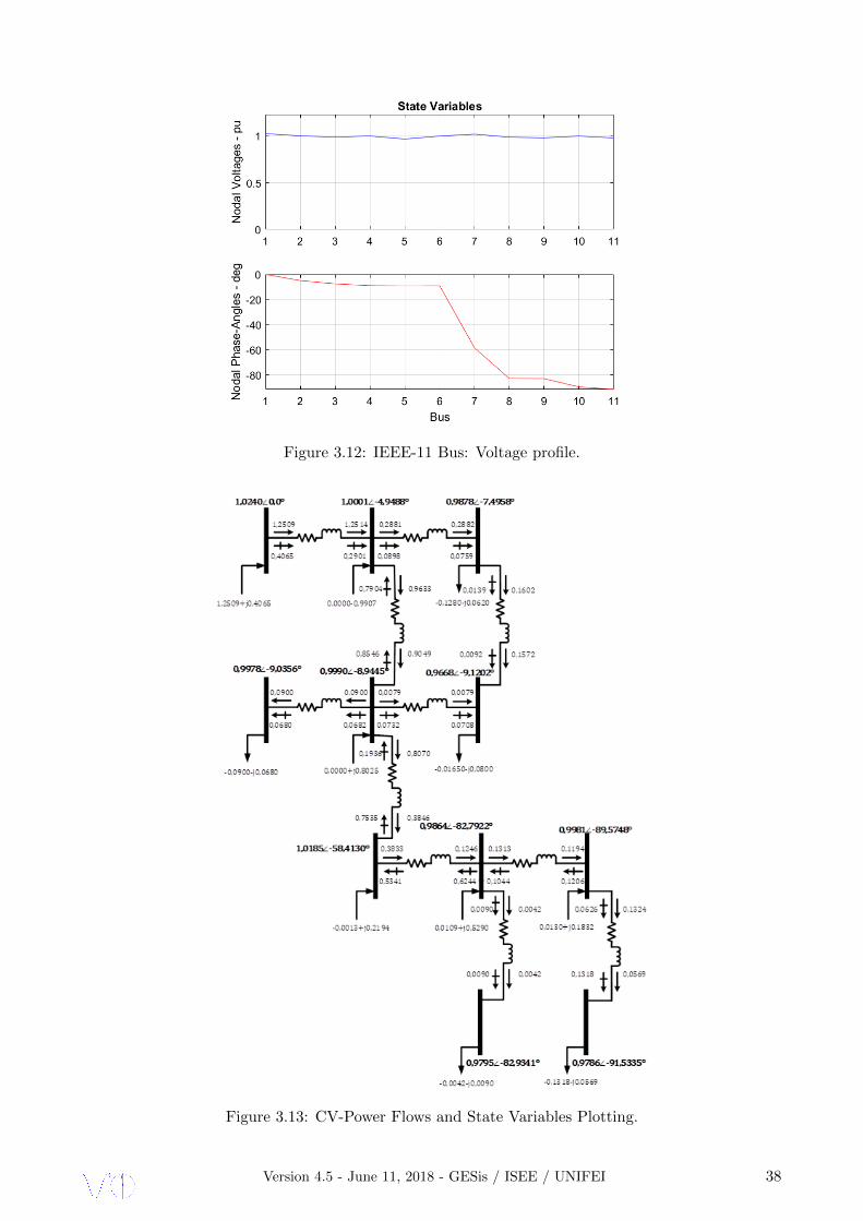
Figure 3.12: IEEE-11 Bus: Voltage profile.

Figure 3.13: CV-Power Flows and State Variables Plotting.


4 Complex-Valued Power System State Estimation - (CV-PSSE)

4.1 Introduction

With the deployment of wide-area synchrophasor measurements that provide metered values of

voltage and current phasors of a power system and the installation of power electronic devices such

as FACTS devices and HVDC links, the formulation of power system state estimation in the complex

domain becomes an important research topic [46], [47], [48].

Optimization problems in the complex domain are frequently encountered in applied mathematics

and in signal processing [49], [11], [6], [10], [50], in control theory, in artificial neural networks [51], [52],

and in biomedicine, to name a few. In power systems, a few papers have been recently published that

deal with power flow calculations for power transmission and distribution systems modeled in the

complex domain using both iterative and non-iterative methods [17], [16], [18], but none in power

system state estimation. The solution methods of these problems often require a first- or second-order

approximation of the objective function. However, such methods cannot be applied to real functions of

complex variables because they are non-analytic in their arguments and therefore, for these functions

Taylor series expansions do not exist. To overcome this difficulty, the objective function is usually

redefined as separate functions of the real and imaginary parts of its complex arguments so that

standard optimization methods can be applied. Although not widely known, it is also possible to

construct an extended objective function that includes not only the original complex state variables,

but also their complex conjugates and then apply the Wirtinger calculus [2], [3]. This property lies on

the fact that if a function is analytic in the space spanned by <x and =x in R, it is also analytic

in the space spanned by x and x* in C.

In complex analysis of functions of complex variables, the Wirtinger operators are partial dif-

ferential operators of the first order that are similar to the ordinary derivatives with respect to real

variables. These operators allow the construction of a differential calculus of functions of complex vari-

ables that is entirely analogous to the ordinary differential calculus of functions of real variables [4]. In

this thesis, we take advantage of the fact that the power flow equations on which the state estimation

model relies lends itself well to a complex-valued formulation to derive the solution for the complex-

valued power system state estimation that minimizes a WLS criterion using the Wirtinger calculus.

Finally, we derive a Gauss-Newton iterative algorithm for solving the complex-valued power system

state estimation problem while using the QR-factorization of the complex-valued Jacobian matrix.

The remaining part of the section is organized as follows. Subsection 2 provides a formal in-

troduction to the complex-valued power system weighted-least-squares state estimation, including

the derivation of the nonlinear measurement model; the Gauss-Newton algorithm; the high-order

Levenberg-Marquardt algorithm; the QR algorithm as applied to the PSSE problems with emphasis

to the direction of maximum rate of change of the cost function, all in conjugate coordinates. Finally,

the Subsection 3 describes two QRD-algorithms, both addressed for the factorization of matrices in

the C-domain.


4.2 Complex-Valued WLS Power System State Estimation

4.2.1 Complex-Valued Nonlinear Measurement Model

In this work, the nonlinear model of the measurements includes additive errors that follow a complex

multivariate Gaussian distribution as proposed by Van Den Bos [53]; the reader is referred to [49], [50]

and [54] for further details on the subject matter. Let zc denote a measurement vector of complex

random variables defined in the complex conjugate coordinate as

zc = (z1 · · · zm, z∗1 · · · z∗m)T , zc ∈ C2m×1 (156)

with

zi = ai + j bi and z∗i = ai − j bi, (157)

where ai, bi ∈ R. Moreover, we assume that the real variables ai and bi, for i = 1, · · · , m, are

normally distributed. Therefore, the power system state estimation nonlinear model in the C-domain

is expressed as

zc = hc (xc) + ωc, (158)

E(ωc) = 0, E(ωc ωHc ) = Ωc. (159)

where zc = (z, z∗) is a vector of complex-valued measurements of dimension (2m × 1); xc = (x,x∗)

is a vector of complex-valued state variables of dimension (2n × 1); hc(xc) is a vector of nonlinear

functions of dimension (2m× 1) that maps zc to xc; ωc is a vector of a complex measurement random

errors of dimension (2m× 1); Ωc is a Hermitian positive-definite covariance matrix of ωc of dimension

(2m × 2m). The superscript (·)H stands for Hermitian operator, that is, the transpose complex

conjugate operation.

4.2.2 Complex-Valued Gauss-Newton Algorithm

As shown in [6], the complex-valued WLS state estimator minimizes an objective function defined as

argminxc

J (xc) =1

2(zc − hc(xc))

H Ω−1c (zc − hc(xc)). (160)

The necessary condition of optimality is given by

∂J (xc)

∂xc= −H(xc)

H Ω−1c (zc − hc(xc)) = 0. (161)

By applying a first order Taylor series expansion of hc(xc) about x(ν)c , we get

hc(xc) = hc(x(ν)c ) + H(x(ν)

c ) (xc − x(ν)c ). (162)

By replacing (162) into (161), we obtain

H(x(ν)c )

HΩ−1c

[zc − hc(x

(ν)c )−H(x(ν)

c ) (xc − x(ν)c )]

= 0, (163)

yielding the updated estimated state vector expressed as

x(ν+1)c = x(ν)

c + G(x(ν)c )−1

H(x(ν)c )

HΩ−1c ∆z

(ν)c , (164)


where G(x(ν)c ) = H(x

(ν)c )

HΩ−1c H(x

(ν)c ) and ∆z

(ν)c = zc−hc(x

(ν)c ). The iterations are stopped when∣∣∣∣∣∣∆x

(ν)c

∣∣∣∣∣∣∞≤ tol, e.g., 10−3, (165)

where ‖·‖∞ is the infinity norm and ν is the iteration counter.

Note that in (161), H(xc) is the Jacobian matrix of dimension (2m× 2n) defined in the complex

domain as

H(xc)∆=∂hc(xc)

∂xc

∆=

∂hc(xc)∂x

∂hc(xc)∂x∗

∂h∗c(xc)∂x

∂h∗c(xc)∂x∗

. (166)

Let Jh =∂hc(xc)∂x and Jd

h =∂hc(xc)∂x∗ be Jacobian submatrices of dimension (m × n). They are

obtained through the Wirtinger partial derivatives with respect to the complex and the complex

conjugate state vector using the rule stated in (17) and (18), respectively. Let us define the Jacobian

matrix as

Jc(xc) = (Jh Jdh). (167)

In the important special case given by (160) where J (xc) is a real-valued function of complex variables,

the following property holds:

J (xc) ∈ R⇒ ∂h∗c(xc)

∂x=

(∂hc(xc)

∂x∗

)∗=(Jdh

)∗. (168)

Therefore, taking into account the rule expressed in (48) and the property stated in (168), (166)

becomes

H(xc) =

(Jh Jd

h

(Jdh)∗ (Jh)∗

)=

(Jc(xc)

J∗c(xc) S

), (169)

where S is a swap operator that permutes blocks of m rows or blocks of n columns depending upon

whether S pre-multiples or post-multiples a matrix, respectively. Moreover, this operator is an iso-

morphism from C to the dual space C∗, which obeys the properties S−1 = ST = S. It shows that S is

symmetric and is equal to its own inverse, that is, S2 = I. For instance, as shown in [5], this matrix

is defined as

S∆=

[0 In

In 0

], (170)

where In is the (n× n)-identity matrix.

Now, the complex-valued gain matrix G(xc) is expressed as

G(xc) =

(Gx x Gx∗ x

Gx x∗ Gx∗ x∗

), (171)

where Gx∗ x∗ =(Gx x

)∗and Gx∗ x =

(Gx x∗

)∗, all of dimension (n× n). Then, it follows from (168)

that

Gx x =

= 12

[(∂h∂x

)HΩ−1c

(∂h∂x

)+

((∂h∂x∗

)HΩ−1c

(∂h∂x∗

))∗],

= 12

[Jh

H Ω−1c Jh +

(Jd

hH

Ω−1c Jd

h

)∗],

(172)


Similarly, we get

Gx∗ x =

= 12

[(∂h∂x

)HΩ−1c

(∂h∂x∗

)+

((∂h∂x∗

)HΩ−1c

(∂h∂x

))∗],

= 12

[Jh

H Ω−1c Jd

h +(Jd

hH

Ω−1c Jh

)∗].

(173)

4.2.3 Complex-Valued High-Order Levenberg-Marquardt Algorithm

As stated before, the key idea is to enhance the condition number of the complex-valued Jacobian

matrix when updating the estimated state variables in (176), yielding

∆x(ν)c =

(H(xc)√η I

)† (∆zc0

), (174)

where η > 0 is the Levenberg-Marquardt regularization parameter which influences both the length

and direction of the update to be added to the estimated variables that minimize the objective function.

Notice that the † operator is defined as the Moore-Penrose pseudoinverse [42]. A detailed derivation

regarding this enhancement that adds numerical robustness and better performance to the power

system state estimation, regardless the coordinate numbers domain, can be found in our paper [55].

4.2.4 Complex-Valued PSSE Numerical Solutions

The complex-valued power system state estimation numerical solution is addressed by solving the

weighted form of the right-hand side (rhs) of (161), yielding

H(xc) ∆x(ν)c = ∆zc, (175)

where H(xc) = Ω−1/2c H(xc) is of dimension (2m×2n) and ∆zc = Ω

−1/2c ∆zc is of dimension (2m×1).

The incremental change in the state vector is calculated via

∆x(ν)c = H(xc)† ∆zc, (176)

where the † operator is defined as the Moore-Penrose pseudoinverse [56].

Two QR-algorithms in the C domain based on the Givens rotations and as described in [7], [8] have

been implemented and tested. Similarly, the well-known real-valued algorithm proposed in [26] and

applied to PSSE by [27], [28], and [29] can be accordingly converted to the complex domain. To avoid

explicitly storing the Q-matrix, we apply the QR-transformation to the augmented matrix, Ha(xc),

given by

Ha(xc) =[H(xc) ∆zc

]. (177)

By storing the rotations in compact form the complex-valued Jacobian matrix can be kept constant

and only the right-hand-side vector is updated throughout the final iterations. The solution of the

state vector increment given by (176) is found by executing a simple back-substitution of (177) after

performing unitary transformations to the latter matrix, resulting in

Ha(xc) =[Tc ∆˜zc] . (178)


Here, Tc is an upper triangular matrix of dimension (2n× 2n) and ∆˜zc comprises the corresponding

rows in the updated RHS vector of dimension (2n × 1). Finally, (176) is solved by performing a

back-substitution via

∆x(ν)c = Tc ∆˜zc. (179)

Note that when executing the algorithm given by (179), only the complex conjugate state vector,

x∗, has to be updated. Indeed, in the sequel is shown that the complex conjugate gradient gives the

direction of maximum rate of change of the cost function. Therefore, the steps defined in (165) and

(179) can be numerically decoupled; consequently, only the Jacobian matrix as stated in (167), i.e.,

associated with ∆z(ν)c = zc − hc(x

(ν)c ), has to be stored and factorized. It becomes possible because

the Jacobian matrix is redundant and has a very nice property as stated in (168) and also showed in

(169). In the sequel this issue is better clarified and explored.

4.2.5 Direction of Maximum Rate of Change of the Cost Function

As shown by Bonet [11], the necessary and sufficient conditions satisfied by the minimum point of

the WLS objective function, J (xc), given by (160) with respect to a complex vector xc are expressed

as

∇xhc(xc) = 0, (180)

∇x∗hc(xc) = 0. (181)

They state that the cogradient and the conjugate cogradient of J (xc) are equal to zero at the

minimum point. Consequently, any small change in the state vector, ∆xc, may or may not result in

a change in the cost function value depending on the search direction. In the C domain, Bonet [11]

proved that the direction of maximum rate of change of the cost function is that of the cogradient

given by (181). Let us summarize the main steps of Bonet’s proof by using the differential rule given

by (48) for vectors, which leads to

dhc =(∇xc

hc(xc))T

dxc +(∇xc

∗ hc(xc))T

dxc∗ ∈ R. (182)

Identifying the expression ∇a = 12(∇xc

+∇xc∗) of the real part of a complex vector results in

dhc = 2×<(∇xc

hc(xc))T

dxc

, (183)

By applying the multivariate equivalent property stated in (168) to (183), we get

dhc = 2×<(∇x∗c hc(xc)

)Hdxc

. (184)

which is proportional to the inner product of two complex-valued vectors, ∇xc∗ hc(xc) and dxc. When

the vectors ∇xc∗ hc(xc) and dxc are orthogonal, then the inner product is null, which makes the rate

of change of the cost function to vanish at a stationary point. Recall that in this special case the

cogradient vector ∇xc∗ hc(xc) is orthogonal to the contours of the cost function as shown in Fig. 2.1.

4.2.6 Numerical Decoupled Solutions

Two algorithms are proposed aiming to mitigate the computational overhead, i.e., the iterative

searching for the final state variables vector. Both are based on the very nice properties stated in


(168) and (184). These properties allow us to decouple the numerical solution of the weighted form

referred to the right-hand side of (161) yielding

Jc(xc)(ν) ∆xc

(ν) = ∆z(ν), (185)

which in expanded form leads to

Ω−1/2[Jh Jd

h

](ν)(

∆x(ν)

∆x∗(ν)

)= Ω−1/2 ∆z(ν), (186)

where Ω−1/2 and(Jh Jd

h

)are of dimension (m×m) and (m×2n), respectively. Moreover, ∆z(ν) = z−

h(x(ν)). Thus, the solution of (186) allows to update the state variables for the first time at current

iteration, as

xc(ν) = xc

(ν−1) + ∆x(ν)c , (187)

Similarly, the other half linear system of equations in (161) is given by

Jc∗(xc) S ∆xc

(ν) = ∆z∗(ν) (188)

where S is a swap matrix which post-multiples Jc∗(xc), yielding

(Ω−1/2

)∗ [(Jd

h)∗ (Jh)∗](ν)

(∆x(ν)

∆x∗(ν)

)=(Ω−1/2

)∗∆z∗(ν), (189)

thus, the solution of (189) updates the state variables vector for the second time at the current

iteration, yielding

xc(ν) = xc

(ν−1) + ∆x(ν)c . (190)

The steps (185-190) is the algorithm called complex-valued fast decoupled state estimation, CV-

FDSE for short, which allows to speed up the convergence process once the state variables vector is

twice updated at each iteration.

On the other hand, the second algorithm is based just on the two first steps of CV-FDSE, i.e.,

(186-187), because the solution obtained through this sub-system of equations depicts the direction of

maximum rate of change in the cost function (see Fig. 2.1).

In this thesis, the results produced by these two algorithms are not presented but will be discussed

in the forthcoming papers.

4.3 Complex-Valued Factorization Algorithms

Two QR-Decomposition (QRD) algorithms are investigated in this thesis. The first one is the

Three-Angle Complex Rotations (TACR), which is derived in polar coordinates [7] whereas the second

algorithm is based on the Fast Plane Rotations [8] that is derived in complex plane. Both approaches

are presented in the the sequel. Nonetheless, we have recommended the TACR algorithm for perform-

ing the Jacobian matrix factorization in C−domain because it is very easy encoding. Notice that both

algorithms are derived from their counterpart in R− domain [26]. Thus, one believe that both follow

the same standards of fill-in suppression when ordering schemes addressed for QR−decomposition in

real domain are applied. Nonetheless, this issue should be investigated later. In this sense, the set of

algorithms reported in [57] should be tried in C−domain, besides news ones proposed in the updated

state-of-the-art, e.g., [58], [59].


4.3.1 Three-Angle Complex Rotation Algorithm

The TACR algorithm is aQR−Decomposition (QRD) unitary transformation (not orthogonal!..)

because it operates in complex domain. Aiming this target, consider the following complex matrix

H2×2 defined by

H2×2 =

[A ejθa C ejθc

B ejθb D ejθd

](191)

where j =√−1; A, B, C, D represent the magnitude and θa, θb, θc, θd stand for the angle of the

matrix entries.

The complex Givens rotations is described by two rotation angles θ1, θ2, through the following

matrix transformation:[cos θ1 sin θ1 e

jθ2

− sin θ1 e−jθ2 cos θ1

][A ejθa C ejθc

B ejθb D ejθd

]=

[X ejθx Y ejθy

0 Z ejθz

](192)

where angles θ1, θ2 are chosen to set to zero the matrix element below the main diagonal, and are

defined by

θ1 = tan−1(B/A)

θ2 = θa − θb(193)

It is easy to verify that using (193) leads to an upper triangular matrix with complex diagonal

elements (192).

On the other hand, an alternative approach for the aforementioned QRD may be realized through

a unitary matrix transformation which can be reached as follows:

Z =

[cos θ1 e

jθ2 sin θ1 ejθ3

− sin θ1 e−jθ2 cos θ1 e

jθ3

](194)

where

θ1 = tan−1(B/A)

θ2 = −θaθ3 = −θb

(195)

Remark that in (195) the three angles that give a name to the algorithm are function of Aejθa and

Bejθb , i.e., depend only of two planes to be rotated. Then, the suggested TACR technique results in

a new triangular matrix as showed below:

[cos θ1 e

jθ2 sin θ1 ejθ3

− sin θ1 e−jθ2 cos θ1 e

jθ3

][A ejθa C ejθc

B ejθb D ejθd

]=

[X Y ejθy

0 Z ejθz

], (196)


Note that the TACR matrix transformation in (196) introduces the real element X on the matrix

diagonal. Application of the TACR approach for an n× n matrix will lead to the appearance of real

elements on the matrix diagonal except for the lowest one.

In order to avoid complex division, for instance, when doing the backsubstitution step within the

solution of linear system of equations, it is advantageous to eliminate the complex lowest diagonal

element. Therefore, aiming this target, the further simple unitary transformation is required:

[1 0

1 e−jθz

][X Y ejθy

0 Z ejθz

]=

[X Y ejθy

0 Z

]. (197)

On the other hand, the aforementioned additional unitary transformation can be needless if the

TACR algorithm operates over an augmented coefficient matrix (178) aiming the solution of the same

linear system of equations. In other words, it means that the original coefficient matrix should be

added of one column comprised by the right hand side of the linear system of equations to be solved.

Consequently, the lowest diagonal element of the coefficient matrix naturally appears as a real number.

4.3.2 Complex-Valued Fast Givens Rotations

The complex-valued fast Givens rotations (CVFGR) is a very interesting algorithm aiming a QR-

Decomposition of matrices once the computations are performed incrementally, i.e., as the data arrives

sequentially in time [8]. It allows us to reduce the overall latency and hardware resources drastically.

In the forthcoming papers, the TACR; the CVFGR and those which are well known because they were

successfully applied to power system state estimation by [27], [28], and [29], once they are accordingly

converted from real- toward complex-domain, their performance will be compared.


5 Complex-Valued Bad Data Processing

Complex-valued signals have been applied to a great number of research areas, such as commu-

nications; radar; echocardiogram images; features for face recognition; geophysics, optics, and electro-

magnetics, to name a few [49]. Nowadays, in power area the electric companies around the world have

deployed a large number of synchro-phasor measurement units (PMUs) for monitoring their power

transmission systems. Hence, the PMU measurement is an enough motivation to extend the model

of complex random variables towards the whole system of measurements in an Energy Management

System (EMS). In this sense, a common assumption that is taken when dealing with complex random

signals is that they are proper or circular, which implies that some aspect of the statistics of a complex

signal is ignored [60], [61], [62], [63], [64]. A proper complex random variable is uncorrelated with its

complex conjugate, and a circular complex random variable has a probability density function (pdf )

such that for any α, the pdf of Z and Z ′ = ejαZ are invariant [60]. Although, these assumptions

are mathematically convenient targeting low computational overhead, there are also many situations

where proper and circular signals are very poor models of the underlying physics. To exploit the

improper or noncircular nature of signals, the complete statistical characterization of complex-valued

random signal, e.g., the complementary correlations (or pseudo-) correlation is required.

This section is organized as follows. Subsection 2 defines the nature of complex random signals.

Subsection 3 presents the complex-valued multivariate generalized Gaussian distribution (CV-GGD).

Subsection 4 presents the complex linear and nonlinear models of measurements. Subsection 5 shows

the derivation of bad-data processing, detection and identification methods in complex domain. In

Subsection 6 is presented the numerical results as applied to a small example and large systems as

showed before within this section. Finally, in Subsection 7 some partial conclusions are stated.

5.1 Nature of Complex Random Signals

Considering a complex random variable z = zR + j zI , besides the covariance matrix calculation

given by

Cc = E[zzH ] = E[z2R] + E[z2

I ] = σ2R + σ2

I , (198)

it is also necessary to include the so-called pseudo-covariance matrix [65], yielding

Pc = E[zzT ],

= E[zR2]− E[zI

2] + 2j E[zRzI ],

= σ2R − σ2

I + 2jρ,

(199)

where σ2 is the variance and ρ is the correlation E[zRzI ]. Then, under such condition a complex

Gaussian random signal is called second-order circular iff it is zero-mean and proper and its variance

is twice the variance of real and imaginary parts: σ2 = 2 σ2R = 2 σ2

I . However, among other many prac-

tical reasons, being the most common that due to short observation windows, the pseudo-covariance

matrix should be taking into account, i.e., Pc 6= 0. Thus, to cater for noncircularity, the literature in

signal processing [61], [62], [63] have recommended the signal model based on the complex variable in

the complex conjugate coordinate, i.e.


Z = M

[zR

zI

]=

[z

z∗

], (200)

where the matrix M ∈ C2×2 is defined as

M =

1 j

1 −j

, (201)

being j =√−1, and for what follows it is important to note that

M−1 =1

2MH . (202)

Thus, the following covariance matrix [65] can be defined

Ωc = E[Z ZH ] =

Cc Pc

P∗c Cc∗

, (203)

where (·)∗, (·)T and (·)H denotes the complex conjugate, complex transpose and complex conjugate

transpose (Hermitian matrix), respectively. Therefore, both second-order circular and noncircular

nature of signals can be modeled for general complex processes. Remark that the Ωc matrix in (203)

will have real-valued diagonal elements while complex-valued off-diagonal elements. For Z as defined

in (200) to be second-order circular the variance of ZR and ZI are the same and ZR and ZI are

uncorrelated. In this sense, a measure of second-order noncircularity is known as [66]

The degree of impropriety =|E[Z2]|E[ZZ∗]

, (204)

with bounds 0 ≤ |E[Z2]|/E[ZZ∗] ≤ 1, while |E[Z2]| = 0 indicates circular data. Furthermore, in the

complex signals processing literature the circularity measure ξ is proposed as the ratio between the

standard deviation of the real and imaginary components of the signal [67]

ξ =

√σZR

σZI

. (205)

where the value of ξ = 1 indicates equal powers in the real and imaginary components and thus a

proper signal, whereas ξ > 1 indicates improperness.

Summing up, observe that circularity implies zero mean and propriety, but not vice versa. Either,

impropriety implies noncircularity, but not vice versa.

5.2 CV-Multivariate Generalized Gaussian Distribution

As aforementioned, the complex statistics are not a straigthforward extension of real-valued statis-

tics. Then, let us consider the distribution of samples from a complex process in which the real and

imaginary parts are Gaussian distributed. The key concept herein is to derive a compact form of the

density function which can be written directly as a function of a complex argument rather than its

real and imaginary parts. In this sense, a collection of m complex numbers is simply a collection of

2 ×m real numbers. Thus, a collection of m complex random variables is really just a collection of


2×m real random variables with some joint distribution (density) of its real and imaginary parts in

R2m.

Firstly, let us taking into account a vector η ∈ R2m×1 as the corresponding random error of

measurements as defined in real domain, i.e.,

η =(ηR1

, ηI1 , · · · , ηRm, ηIm

)T, (206)

and E[ηRi

]= E

[ηIi

]= 0 for all i. In other words, the random errors have a Gaussian distribution

and are samples of a circular and proper complex stochastic process. Then, the covariance matrix of

η can be defined as

R = E[η ηT

]. (207)

The distribution function of ηRiand ηIi is described by

f(η) =1

(2π)m (det R)1/2e(− 1

2ηT R−1 η). (208)

On the other hand, based on what was stated in (200) and equation (208), follows that

ωi

ω∗i

= M

ηRi

ηIi

, (209)

where ωi = (ηRi+ j ηIi ) and M is defined as in (201). Now, defining ωc ∈ C2m×1 as the random error

of measurements in the complex conjugate coordinate becomes

ωc = (ω1, ω∗1, · · ·ωm, ω∗m)T . (210)

Then, by (209) yields

ωc = A η, (211)

where the block-diagonal matrix A ∈ C2m×2m is defined as

A = diag (M,M, · · · ,M) . (212)

Hence, by (211) and (202) results

η = A−1 ωc =1

2AH ωc, (213)

and since η is a real vector, thus

η =1

2AT ω∗c . (214)

The covariance matrix Ωc ∈ C2m×2m of ωc, by (211) becomes

Ωc = A R AH . (215)

Now, let us consider the quadratic form in (208) as in [53], yielding


ηT R−1 η. (216)

By (213), (214) and (215) this form may be written as

ωHc (12A) R−1 (1

2AH) ωc = ωHc(A R AH

)−1ωc,

= ωHc Ω−1c ωc.

(217)

Moreover, the determinant in (208) may be written as

det R = det(12AH Ωc

12A),

=(

12

)2m (det MH

)mdet Ωc

(12

)2m(det M)m ,

=(

12

)4m(2j)m (−2j)m det Ωc,

=(

12

)2mdet Ωc.

(218)

Substitution of (217) and (218) in (208), allow to obtain the complex-valued multivariate generalized

Gaussian distribution, yielding

f(ωc) =1

πm(det Ωc)e(−ωH

c Ω−1c ωc). (219)

with ωc defined by (210). Moreover, note that the pdf depends algebraically on ωc, i.e., ωi and ωi∗,

but is interpreted as the joint pdf of ηRiand ηIi , and can be used for proper and improper ωi. Now,

it is straightforward to introduce a non-zero mean µ, which is the complex vector isomorphic to the

mean of its real counterpart. The resulting pdf is

f(ωc) =1

πm(det Ωc)e−(ωc−µ)H Ω−1

c (ωc−µ). (220)

Finally, aiming to meet the definition and format assumed before within this section, recall that

ωc can be rearranged as follows

uc = S ωc = (ω1 · · ·ωm, ω∗1 · · ·ω∗m)T , (221)

where S ∈ R2m×2m is a permutation matrix, which entries are either equal to one or to zero, and the

following property holds: ST = S−1 and |det S| = 1, i.e., S is an orthogonal matrix [68].

In Fig. 5.1 are shown different complex-valued signals nature [69]. This picture shows the scatter

plots for three nature of signals: (a) ice multiparameter imaging -band radar (IPIX) data from the

website http://soma.crl.mcmaster.ca/ipix/; (b) a 16-quadrature amplitude modulated (QAM) signal;

and (c) wind data obtained from http://mesonet.agron.iastate.edu. While Fig. 5.2 depicts their

corresponding covariance functions and complementary covariance functions.


(a) Radar data. (b) 16-QAM data. (c) Wind data.

Figure 5.1: Scatter plots for (a) circular, (b) proper but noncircular, and (c) improper (and thus

noncircular) data.

The radar signal in Fig. 5.2 (a) is narrow-band. Evidently, the gain and phase of the in-phase and

quadrature channels are matched, as the data appear circular (and therefore proper). The uniform

phase is due to carrier phase fluctuation from pulse-to-pulse and the amplitude fluctuations are due to

variations in the scattering cross-section. The 16-QAM signal in Fig. 5.2 (b) has zero complementary

covariance function and is therefore proper (second-order circular). However, its distribution is not

rotationally invariant and therefore it is noncircular. The wind data in Fig. 5.2 (c) is noncircular and

improper.

(a) Radar data. (b) 16-QAM data. (c) Wind data.

Figure 5.2: Covariance and complementary covariance function plots for the corresponding processes

in Fig. 5.1: (a) circular (b) proper but noncircular; and (c) improper.

Further insights regarding the nature of complex random signals can be found in [], [70], [66] [54],

[64], [9], [67], [60], [61], [62], [71], [72]. Near future, our intend is to investigate the nature of the

data set that comes from a low-voltage widearea measurement system consisting of 24 PMUs installed

nationwide in Brazilian university campuses: http://www.medfasee.ufsc.br/temporeal/. Addionally,

key issues should be taken into account when a complex-valued signal is modeled within the state

estimation applications, as presented in [73], [74] and [75], to cite a few.


5.3 Complex-Valued Measurements Models

5.3.1 Complex Linear Model

If the data model is linear, the minimum variance unbiased (MVU) estimator can be easily found [72].

The complex linear model has the form

zc = H xc + ωc, (222)

E(ωc) = 0, E(ωc ωHc ) = Ωc. (223)

where zc is a vector of complex-valued measurements, m×1; H is a known m×n complex observation

matrix and full rank; xc is a complex n × 1 true state variables vector, e.g., (x,x∗), while, ωc is a

m× 1 complex random noise vector with pdf ωc ∼ CN (0,Cc,Pc = 0). Nonetheless, it is well known

that strictly linear transformations of proper complex Gaussian random vectors yield again proper

complex Gaussian distributed random vectors. Thus, zc ∼ CN (E[zc],Cc,Pc = 0), where it can be

shown that E[zc] = H xc and Ωc = Cc. Therefore, the MVU estimator of xc is given by

xc = (HHΩ−1c H)−1HHΩ−1

c zc. (224)

5.3.2 Complex Nonlinear Model

As already stated above, let us assume zc as a measurement vector of a complex random variables

defined as

zc = (z1 · · · zm, z∗1 · · · z∗m)T , zc ∈ C2m×1 (225)

with

zi = zRi + j zIi and z∗i = zRi − j zIi , (226)

where zRi , zIi ∈ R. Moreover, the real quantities zRi and zIi , for i = 1, · · · , m are normal distributed.

Therefore, under these assumptions the nonlinear complex-valued model of measurements referred to

PSSE problem in C-domain can be stated as follows

zc = hc (xc) + ωc, (227)

E(ωc) = 0, E(ωc ωHc ) = Ωc. (228)

where hc is a vector of nonlinear functions that maps a complex-valued measurements, e.g., (z, z∗)

towards a complex-valued true state variables, e.g., (x,x∗). The remaining variables stated in (227)

and (228) are defined as aforementioned and the estimates of xc,i.e., xc, are known as showed before

within this section.

5.4 Complex-Valued Bad Data Detection and Identification Methods

In this work a classical bad data detection and identification methods in power system state estimation

are revisited [76], [77], except that both are herein derived in complex domain.


5.4.1 Detection: Complex-Valued Chi-squared Test

It is well known that a common test performed aiming bad data detection is to compute the

sum of squared magnitudes of the residual vector and compare this to a threshold. The resulting test

statistic has a behavior modeled by the χ2-squared distribution [78].

Thus, let us assume the set of measurements as a m complex Gaussian random variables, inde-

pendent and identically distributed with mean 0 and variance 1 (meaning that the covariance matrix

for the residual vector, rc, is I). Recall that central distributions are usually associated with the null

hypothesis in a detection problem and are used to compute the probability of false alarm. In this

sense, defining the real non-negative random variable J (rc) according to

J (rc) =m∑i

|rci |2. (229)

The density χ2-squared distribution function for J (rc), for simplicity this latter with its argument

omitted, is given by

fJ (J ) =1

(m− 1)!Jm−1 e−J U(J ), (230)

which is derived assuming the pdf for |rci |2 is a simple exponential. Then, Eq. (230) is the m− foldconvolution of this exponential density function with itself [78]. Also, recall that fJ (J ) is a gamma

density function with an integer parameter m, and like the pdf defined in (219), it is cleaner and

simpler than its real counterpart. Likewise, in (230) we often say that J is χ2 with m complex

degrees of freedom. However, note that although a “complex degree of freedom” is like 2 × m real

degrees of freedom, Eq. (230) is not the usual χ2-squared density function with 2×m real degrees of

freedom. Indeed, recall that in (219) each real random variable going into the computation of J has

variance 1/2, not 1 [78], i.e., ∫Cm

fz(z)dz = 1. (231)

The probability that z ∈ κ, where κ is some subset of Cm, is given by

p(κ) =

∫κfz(z)dz, (232)

and the differential element dz is understood to be

dz = dzR1dzI1 dzR2dzI2 . . . dzRmdzIm . (233)

5.4.2 Identification: Largest Normalized Residual Method

The main concern in this method is to becoming known the covariance matrix of residual prior

to normalize the residual vector. Recall that the normalized residual values are obtained through the

weighting of residual values by the corresponding variance values of the residual [77]. Indeed, as the

same assumptions can be assumed aiming the derivation of its counterpart in complex domain through

an equivalent expression, yields∑=[I−H (HH Ω−1

c H)−1HHΩ−1c

]Ωc. (234)


where∑

is the covariance matrix of residual and H is the power system state estimation’s Jacobian

matrix, as defined in (169). Hence, the complex normalized residual values are computed as follows

rni =ri√∑

ii

. (235)

In this sense, only an individual checking of a real and imaginary parts of rni allows to identify

which measurement violates the complex-valued measurement model. Recall that the searching for

the largest normalized residual value can be processed as follows

max |rN | > λ (≈ 2.5). (236)

5.4.3 Bad Data Redemption as Pseudo Measurement

Once a bad data has been identified among the measured quantities, it is advised to rescue the

gross error as a pseudo measurement rather than reject it, and the reasons are twofold:

1. To mitigate the risk of loss of observability;

2. To avoid further computational overhead caused by the refactorization of Jacobian matrix.

In this section the approach aiming to become a gross error toward pseudo measurement after its

redemption is employed as proposed in [79]. In this sense, the following estimates of the magnitude

of the error can be posed

βi =σi∑ii

rni , (237)

Thus, the pseudo-measurement is determined as follows

znewi = zoldi −σi∑ii

rni . (238)

5.5 Numerical Results Without Bad Data Processing

We first solve the complex-valued WLS estimator in a small 2-bus power system and then apply

the solution method to the IEEE 14- and 30-bus systems and to the Brazilian equivalents 340- and

730-bus systems. The small power system example was simulated considering perfect measurements

and a unitary co-variance matrix for the measurement errors. As for the IEEE-test systems and the

two Brazilian equivalent systems, the accuracy assigned to the PMU and the SCADA measurements

are 10−4 and 10−2, respectively.

5.5.1 Small Power System Example

The one-line diagram of a 2-bus system is depicted in Fig. 5.8. The system is provided with

two PMU measurements that meter the nodal voltage magnitudes and phase angles and two real and

reactive power flow measurements, which are identified by means of black bullets and red triangles,

respectively. In Table 5.1, the network parameters are given in pu.

From Fig. 5.8, the complex power injections at both buses are derived as

S1 = V1

[(y∗12 − j bsh12) V ∗1 − y∗12 V

∗2

], (239)


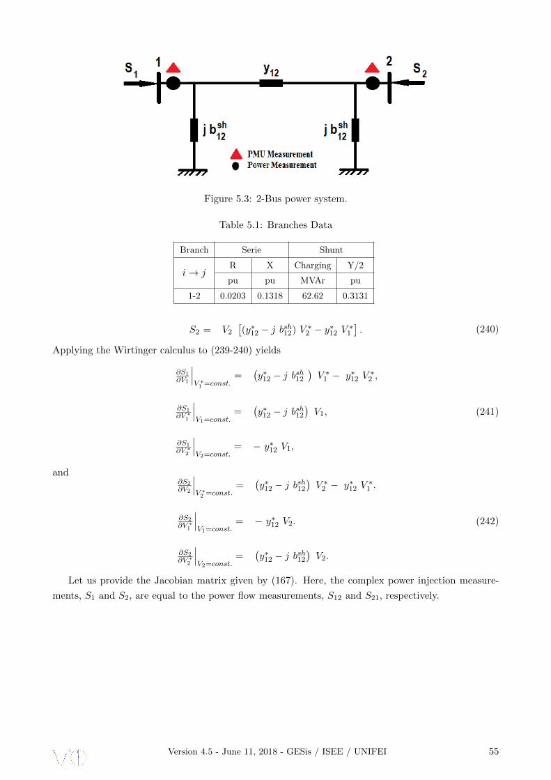
Figure 5.3: 2-Bus power system.

Table 5.1: Branches Data

Branch Serie Shunt

i→ jR X Charging Y/2

pu pu MVAr pu

1-2 0.0203 0.1318 62.62 0.3131

S2 = V2

[(y∗12 − j bsh12) V ∗2 − y∗12 V

∗1

]. (240)

Applying the Wirtinger calculus to (239-240) yields

∂S1∂V1

∣∣∣V ∗1 =const.

=(y∗12 − j bsh12

)V ∗1 − y∗12 V

∗2 ,

∂S1∂V ∗1

∣∣∣V1=const.

=(y∗12 − j bsh12

)V1,

∂S1∂V ∗2

∣∣∣V2=const.

= − y∗12 V1,

(241)

and∂S2∂V2

∣∣∣V ∗2 =const.

=(y∗12 − j bsh12

)V ∗2 − y∗12 V

∗1 .

∂S2∂V ∗1

∣∣∣V1=const.

= − y∗12 V2.

∂S2∂V ∗2

∣∣∣V2=const.

=(y∗12 − j bsh12

)V2.

(242)

Let us provide the Jacobian matrix given by (167). Here, the complex power injection measure-

ments, S1 and S2, are equal to the power flow measurements, S12 and S21, respectively.


Jc(ν=0) =

1.0000

j 0.0000

1.0000

j 0.0000

0.0000 1.1415 - 1.1415

-j 0.3131 j 7.0983 -j 7.4114

0.0000 -1.1415 1.1415

j 0.3131 -j 7.4141 j 7.0983

0.0000 1.1415 - 1.1415

-j 0.3131 j 7.0983 -j 7.4114

0.0000 -1.1415 1.1415

j 0.3131 -j 7.4141 j 7.0983

Jc(ν=1) =

1.0000

j 0.0000

1.0000

j 0.0000

1.8414 0.9145 -0.9145

j 0.2179 j 5.6849 -j 5.9356

-1.7683 -2.5295 2.4565

-j 0.6884 -j 4.9346 j 4.7148

1.8414 0.9145 -0.9145

j 0.2179 j 5.6849 -j 5.9356

-1.7683 -2.5295 2.4565

-j 0.6884 -j 4.9346 j 4.7148

Jc(ν=2) =

1.0000

j 0.0000

1.0000

j 0.0000

1.8683 1.1653 -1.1658

j 0.4802 j 7.1651 -j 7.4813

-1.7962 -2.7074 2.6348

-j 1.0677 -j 6.1598 j 5.8884

1.8683 1.1653 -1.1658

j 0.4802 j 7.1651 -j 7.4813

-1.7962 -2.7074 2.6348

-j 1.0677 -j 6.1598 j 5.8884


Jc(ν=3) =

1.0000

j 0.0000

1.0000

j 0.0000

1.8828 1.1413 -1.1413

j 0.4247 j 7.0982 -j 7.4113

-1.8098 -2.7148 2.6417

-j 1.0085 -j 6.1411 j 5.8704

1.8828 1.1413 -1.1413

j 0.4247 j 7.0982 -j 7.4113

-1.8098 -2.7148 2.6417

-j 1.0085 -j 6.1411 j 5.8704

As observed in the above expressions of Jc, the sub-matrix Jh is more sparse than the sub-matrix

Jdh, which affects the sparsity structure of the complex-valued Jacobian matrix as shown in the sequel.

The state variables at each iteration are provided in Table 5.2, while the estimated measured variables

are given in Table 5.3. The residual vector and the chi-squared index throughout the iterations are

presented in Table 5.4. Note that the estimates values obtained in the C-domain are exactly equal to

those extracted from the power flow report in the R-domain. Furthermore, the Gauss-Newton iterative

algorithm converges in three iterations in both domains.

Table 5.2: Estimated State Variables

Xi

∣∣∣X∣∣∣(ν=0) ∣∣∣X∣∣∣(ν=1) ∣∣∣X∣∣∣(ν=2) ∣∣∣X∣∣∣(ν=3)

V11.0000 1.0097 1.0000 1.0001

e+j 0.0 e−j 0.1015 e+j 0.0018 e+j 0.0004

V21.0000 0.8973 0.8954 0.8956

e+j 0.0 e−j 14.9708 e−j 15.0924 e−j 15.0904

V ∗11.0000 1.0097 1.0000 1.0001

e+j 0.0 e+j 0.1015 e−j 0.0018 e−j 0.0004

V ∗21.0000 0.8973 0.8954 0.8956

e+j 0.0 e+j 14.9708 e+j 15.0924 e+j 15.0904


Table 5.3: CV-Estimated Quantities

zi z(ν=0) z(ν=1) zν=2) z(ν=3)

S120.0000 1.4747 1.8873 1.8827

-j 0.3131 j 0.1745 j 0.4815 j 0.4248

S210.0000 -1.4014 -1.8036 -1.7997

-j 0.3131 -j 0.0707 -j 0.5094 -j 0.4500

S10.0000 1.4747 1.8873 1.8827

-j 0.3131 j 0.1745 j 0.4815 j 0.4248

S20.0000 -1.4014 -1.8036 -1.7997

-j 0.3131 -j 0.0707 -j 0.5094 -j 0.4500

Table 5.4: CV-Residual Vector

CV-Residual Vector

r(ν=i) r(ν=0) r(ν=1) r(ν=2) r(ν=3)

rV10.0000 0.1991 −0.0097 0.0000

j 0.0000 j 0.0000 j 0.0018 −j 0.0000

rV2−0.1349 0.1634 −0.0017 0.0006

−j 0.2333 −j 0.0000 −j 0.0015 −j 0.0001

rS12

1.8827 0.4080 −0.0046 −0.0000

j 0.7375 j 0.2499 −j 0.0571 −j 0.0004

rS21 −1.7998 −0.3984 0.0038 −0.0001

−j 0.1366 −j 0.3790 j 0.0597 j 0.0003

rS1

1.8827 0.4080 −0.0046 −0.0000

j 0.7375 j 0.2499 −j 0.0571 −j 0.0004

rS2

−1.7998 −0.3984 0.0038 −0.0001

−j 0.1366 −j 0.3790 j 0.0597 j 0.0003

J (x)ν=i 14.7654 1.1288 0.013825 8.8× 10−7

5.5.2 IEEE-Test Systems and the Brazilian Equivalent Systems

Table 5.5 provides for the two IEEE-test systems and the two Brazilian equivalent power systems,

the total numbers of the state variables, the PMUs, and the SCADA-based measurements along with

the total numbers of branches . Table 5.6 provides for the four power systems the numbers of non-

zero entries of the Jacobian and the gain matrices along with the number of iterations and the total

computing times of the Gauss-Newton algorithm without the implementation of any sparsity technique.

We investigate the sparsity structure of the augmented Jacobian matrix given by (169). Compar-

ison of Figs. 5.4-5.7 reveal that the Jacobian matrices in the C-domain are sparser than those in the

R-domain [57]. For instance, for the Brazilian equivalent 730-bus system, the Jacobian matrix in the

C-domain has 10,396 non-zero-elements while in the R-domain, it has 18,403 non-zero-elements; it is

about 45% sparser.


0 10 20

0

10

20

30

40

50

60

70

nz = 341

RV

−Ja

cobi

an M

atrix

− IE

EE

−14

Bus

sys

tem

(a)

0 5 10 15 20 25

0

5

10

15

20

25

nz = 365

Gai

n M

atrix

− IE

EE

−14

Bus

sys

tem

(b)

0 10 20

0

10

20

30

40

50

60

nz = 184

Com

plex

Jac

obia

n M

atrix

− IE

EE

− 1

4 B

us s

yste

m

(c)

0 5 10 15 20 25

0

5

10

15

20

25

nz = 240

Hes

sian

Mat

rix −

IEE

E −

14

Bus

sys

tem

(d)

Figure 5.4: Sparsity structure of (a) real-valued Jacobian matrix; (b) real-valued gain matrix; (c)

complex-valued Jacobian matrix; (d) complex-valued Hessian matrix of the IEEE 14-bus system.


0 20 40 60

0

20

40

60

80

100

120

nz = 599

RV

−Ja

cobi

an M

atrix

− IE

EE

−30

Bus

sys

tem

(a)

0 10 20 30 40 50 60

0

10

20

30

40

50

60

nz = 817

Gai

n M

atrix

− IE

EE

−30

Bus

sys

tem

(b)

0 20 40 60

0

20

40

60

80

100

120

nz = 366

Com

plex

Jac

obia

n M

atrix

− IE

EE

− 3

0 B

us s

yste

m

(c)

0 10 20 30 40 50 60

0

10

20

30

40

50

60

nz = 484

Hes

sian

Mat

rix −

IEE

E −

30

Bus

sys

tem

(d)


complex-valued Jacobian matrix; (d) complex-valued Hessian matrix of the IEEE 30-bus system.


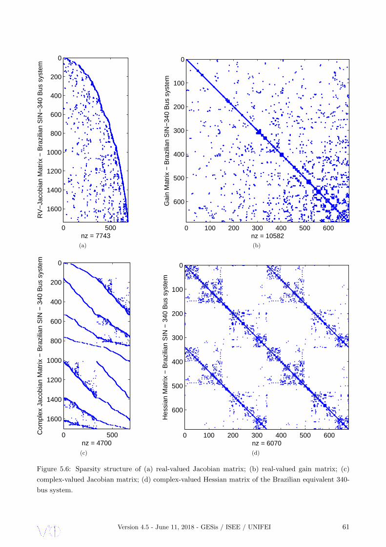
0 500

0

200

400

600

800

1000

1200

1400

1600

nz = 7743

RV

−Ja

cobi

an M

atrix

− B

razi

lian

SIN

−34

0 B

us s

yste

m

(a)

0 100 200 300 400 500 600

0

100

200

300

400

500

600

nz = 10582

Gai

n M

atrix

− B

razi

lian

SIN

−34

0 B

us s

yste

m

(b)

0 500

0

200

400

600

800

1000

1200

1400

1600

nz = 4700

Com

plex

Jac

obia

n M

atrix

− B

razi

lian

SIN

− 3

40 B

us s

yste

m

(c)

0 100 200 300 400 500 600

0

100

200

300

400

500

600

nz = 6070

Hes

sian

Mat

rix −

Bra

zilia

n S

IN −

340

Bus

sys

tem

(d)


complex-valued Jacobian matrix; (d) complex-valued Hessian matrix of the Brazilian equivalent 340-

bus system.


0 500 1000 1500

0

500

1000

1500

2000

2500

3000

3500

nz = 18403

RV

−Ja

cobi

an M

atrix

− B

razi

lian

SIN

−73

0 B

us s

yste

m

(a)

0 500 1000 1500

0

500

1000

1500

nz = 28136

Gai

n M

atrix

− B

razi

lian

SIN

−73

0 B

us s

yste

m

(b)

0 500 1000

0

500

1000

1500

2000

2500

3000

3500

nz = 10396

Com

plex

Jac

obia

n M

atrix

− B

razi

lian

SIN

− 7

30 B

us s

yste

m

(c)

0 200 400 600 800 1000 1200 1400

0

200

400

600

800

1000

1200

1400

nz = 14178

Hes

sian

Mat

rix −

Bra

zilia

n S

IN −

730

Bus

sys

tem

(d)


complex-valued Jacobian matrix; (d) complex-valued Hessian matrix of the Brazilian equivalent 730-

bus system.


5.6 Numerical Results Including Bad Data

In the sequel is presented the application of a classical bad data processing in a small example system

aiming to track its performance in complex-domain. Firstly, the linear complex model of measurements

is considered and compared to those cases discussed in [80]. Likewise, the nonlinear complex model

will be applied to the same 2-bus example system as presented before.

5.6.1 Circular and Proper Complex Linear Model

The one-line diagram of an example system, including the measurement configuration identified by

means of black bullets placed at each measurement point, is shown in Fig. 5.8. All lines are assumed

to have zero resistance and 1.0 pu, reactance, xij .

Figure 5.8: Small 3-Bus Example System.

Taking bus 3 as reference bus (δ3 = 0.0), the problem is to estimate the two bus voltage angles δ1

and δ2 based on a set of 6 real power measurements. Also, namely that the true measurement values

are zero and that the standard deviation of the errors are of 0.01 pu, i.e., Ωc = 10−4 I12×12, which

means a proper and circular data. Then, applying the complex DC model, the contents of equation

(224) to be solved are

Table 5.5: Features of the IEEE-Standards and Brazilian Grids

Number of bus 14 30 340 730

branches 20 41 494 973

states (n) 27 59 686 1560

voltage meas.(V i) 5 11 159 402

active p. flow meas.(tij) 23 34 604 1176

reactive p. flow meas.(uij) 23 34 604 1176

active p. inj. meas.(pi) 11 23 89 241

reactive p. inj. meas.(qi) 11 23 85 260

measurements (m) 73 125 1732 3784


Table 5.6: Parameters and Performance Indices

Number of bus 14 30 340 730

Jacobian Matrix, as in (169):

- Number of rows -> m 30 62 852 1850

- Number of columns -> n 14 30 340 730

Number of nonzero entries in:

- H matrix, as in Eq. (169) -> 184 366 4700 10396

- G matrix, as in Eq. (171) -> 240 484 6070 14178

Number of iterations 3 3 5 6

Total time (s) without sparsity 7.69 10.63 16.93 89.67

Hc = j

1 −1 0 0

−1 1 0 0

1 0 0 0

0 1 0 0

−1 2 0 0

−1 −1 0 0

0 0 −1 1

0 0 1 −1

0 0 −1 0

0 0 0 −1

0 0 1 −2

0 0 1 1

; zc =

0

0

0

0

0

0

0

0

0

0

0

0

; δc = j

δ1

δ2

−δ1

−δ2

.

Strictly speaking, when the data are proper and circular the complex linear model can be solved

likewise its counterpart in real domain. The covariance matrix becomes a diagonal and real-valued

matrix as stated in (198), i.e., Ωc = Cc, although the complex arithmetics have to be used. Other-

wise, i.e., when the pseudo-covariance cannot be neglected (Pc 6= 0), the above formulation must be

employed.

Case A.1:

zc = [0 0 0 0 1 0... 0 0 0 0 1 0]T pu → Measurement 5 is a bad data. The

corresponding normalized residual vector is

zni= [33.0 −33.0 7.5 −24.7 69.5 25.9

... 33.0 −33.0 7.5 −24.7 69.5 25.9]T ∴ It works.

Case A.2:

zc = [0 −1 0 0 1 0... 0 −1 0 0 1 0]T pu → Measurements 2 and 5 are bad data. Both bad

data are not conforming, i.e., not interacted. Thus, the corresponding normalized residual vector is

zni= [7.3 −121.0 −11.2 −17.6 111.3 41.5

... 7.3 −121.0 −11.2 −17.6 111.3 41.5]T ∴ It also works.

Case A.3:

zc = [0 1 0 0 1 0... 0 1 0 0 1 0]T pu → Measurements 2 and 5 are bad data.


But, in this case they are interacting or conforming, and the corresponding normalized residual vector

is

zni= [58.6 55.0 26.2 −31.7 27.8 10.4

... 58.6 55.0 26.2 −31.7 27.8 10.4]T ∴ It fails!... Remark that

the largest residual occurs at measurement 1, which is a good data.

It is now time to give some insights regarding the existence of leverage points in complex domain,

even if this issue is beyond of this work now. Aiming this purpose, let us take the same simulation of

bad leverage points discussed in [81] and carried out in the example system presented in Fig. 5.8 as

showed in the sequel,

Case A.4:

zc = [0 0 −0.55 0 0 1... 0 0 −0.55 0 0 1]T pu → Measurements 3 and 6 are

bad leverage points.

zni= [21.1 −21.1 −6.2 34.0 18.1 30.8

... 21.1 −21.1 −6.2 34.0 18.1 30.8]T ∴ It fails!... Remark

that the largest residual occurs at measurement 4, which is a good data. And, the identification by

elimination based on largest |rni | leads towards next case.

Case A.5:

zc = [0 0 −0.55 0 1... 0 0 −0.55 0 1]T pu → Measurements 3 and 6 are bad

leverage points and measurement 4 is suppressed as suggested in Case A.4.

zni= [18.4 −18.4 −2.0 32.2 17.3

... 18.4 −18.4 −2.0 32.2 17.3]T ∴ It fails again!... Now the largest

residual occurs at measurement 5, which is a good data.

5.6.2 Circular and Proper Complex NonLinear Model

The one-line diagram, including the measurement placement, is shown in Fig. 5.9. Recall it is that

presented before and within this section. Therefore, the whole set of results are already known,

including the intermediary ones.

Figure 5.9: Small 2-Bus Example System.

The main concern here is to extend the application of the classical bad data processing algorithms

towards nonlinear model of measurements in complex domain. In this sense, we are going to consider

bad data regardless it is in real or imaginary parts, being both uncorrelated and have equal variances

of a complex data. Thus, it is intended to simulate bad data in two classes of measurements. Firstly,

we are going to consider as a bad data a complex power simulated as follows:


Case B.1:

zc =

Vk

Vm

Skm

Smk

=

1.0000 + j0.0000

0.8651− j0.2333

−1.8827 + j0.4244

−1.7998− j0.4497

,where the active power (real part) of the complex power at the sending end terminal, i.e., Pkm =

<(Skm) is a bad data.

rni=

12.9295 + j11.1486

6.1186− j14.5367

−185.5201 + j20.0240

−183.3210 + j18.3333

.The complex normalized residual vector showed above points out the bad data properly.

Case B.2:

The real part of the voltage at the receiving end of the Pi-circuit, i.e., <(Vm) is a bad data.

zc =

Vk

Vm

Skm

Smk

=

1.0000 + j0.0000

−0.8651− j0.2333

1.8827 + j0.4244

−1.7998− j0.4497

,and the corresponding complex normalized residual vector allows to identify the bad data correctly.

rni=

49.6222 + j53.3528

−100.4777 + j34.5800

9.0977− j33.8791

−16.1844− j40.5206

.

Case B.3:

The imaginary part of the voltage at the receiving end of the Pi-circuit, i.e., =(Vm) is a bad data.

zc =

Vk

Vm

Skm

Smk

=

1.0000 + j0.0000

0.8651 + j0.2333

1.8827 + j0.4244

−1.7998− j0.4497

.and the corresponding complex normalized residual vector is,


rni=

1.5464− j23.0929

−4.2318 + j25.5528

1.3930 + j 1.2796

−1.0985 + j 2.0941

,and it clearly works.

5.6.3 Noncircular/Proper Complex NonLinear Model

The deployment of a large number of synchro-phasor measurement units (PMUs) for monitoring

power transmission systems around the world is a newly trend [82]. Definitively, a hybrid monitoring

system is already a reality at EMS of many utilities in most of the countries. This is an enough

motivation for investigating statistical models able to better deal with this new endeavour. The PMU

statistical model cannot overlook the fact that a malfunction in whichever voltage or current channels

implies in errors which may violate the measurement model and give rise to a bad data. As we are

dealing with complex signals, then the error in the real and imaginary parts are correlated, thus the

complex signals are non-circular.

5.6.4 Noncircular/Improper Complex NonLinear Model

Not available yet.


The power system weighted-least-squares estimator in the C-domain has been formulated using

the Wirtinger calculus. The estimator has been solved through the complex-valued Gauss-Newton

iterative algorithm. The sparsity structure of the Jacobian and the Hermitian matrices has been

investigated on two IEEE test-systems and the Brazilian equivalent 340- and 730-bus system. As a

future work, partial factorization of the Jacobian matrix will be investigated and residual statistical

analysis for bad data detection and identification will be developed.

In this thesis is derived a covariance matrix which contains information from both the covariance

and pseudo-covariance matrices. This approach allows to deal with any nature of a complex random

variables, e.g., regardless they are proper or improper, circular or non-circular. The classical bad

data processing when applied in complex coordinates behaves likewise in real domain. Nonetheless,

highlights that we are just starting the investigation of keys issues in complex-valued power system

state estimation.

Definitively, complex random signals play an increasingly important role in array, communications,

and biomedical signal processing and related fields. The wider deployment of complexvalued signal

processing is often hindered by the fact that the concepts, tools and algorithms for handling complex-

valued signals are lacking, or, are simply too scattered in the literature. Due to extensive research

in this area during the past few years, as reviewed here, these obstacles no-longer exist, or, are at

least less pronounced. We also wish to point out that due to lack of space, several important topics

in complex-valued signal processing were not discussed here.


6 General Conclusions

In this thesis a new framework in C− domain specially addressed for nonlinear Power Flow

Analysis (CV-PFA) and Power System State Estimation (CV-PSSE) problems is derived. The main

features of these classical tools usually employed for planning electrical network expansion and its

operative security supervision, respectively, are highlighted from Section 3 to 5. But the whole math-

ematical fundamentation that is based on Wirtinger’s Work [3], is outlined in Section 2. In Sections

3 and 4 the main qualitative and numerical analysis obtained till now are presented and discussed.

Therefore, it shall deem advisable that some insights should pointed out towards next steps of this

research, as follows:

1. The Matlab code regarding the CV-PFA should be generalized in order to exploit the sparsity

features and potentially speed up the solution of the problem as it is already done for the

CV-PSSE after the proposed enhancements have been embedded.

2. Besides the adoption of recommended actions stated before, the bad data processing, i.e., the

— classical approach for detection and identification of gross errors in C − domain should be

extended to robust methods. For instance, SHGM estimator [57].

3. Moreover, the behavior of CV-Power Flow and CV-Power System State Estimation algorithms

should be investigated when applied to unbalanced polyphase distribution systems.

4. This Thesis may become a draft of a near future Chapter or even a Book on Complex-Valued

Steady-State Models as Applied to Power Systems Problems - Power Flow Analysis and Power

System State Estimation - intended to be published in English aiming the whole Power and

Energy Society, i.e., Academy and Power Industry community.

6.1 Future Investigations

It seems opportune to outline the near future trends and works to be done based on the framework

proposed in this thesis. The complex-valued power flow and complex-valued power system state

estimation open up the path for embed toward new smart grid technologies.

Definitively, power electronic devices are already a reality in modern power system control. For

instance, VSC-STATCOM and VSC-HVDC [46], [83], [47], [84] and [85] to cite a few. In this sense,

as a future research, we will initiate a power flow framework for hybrid AC-DC systems that include

a variety of FACTS devices, including VSC-HVDC links and STATCOM devices, and will develop

solution methods that are both numerically robust and compatible with real-time applications.

Consequently, the monitoring hybrid network requires advances on PMU and SCADA technolo-

gies [75], [48] and [74]. The power system weighted-least-squares estimator in the C-domain has been

formulated using the Wirtinger calculus. The estimator has been solved through the complex-valued

Gauss-Newton iterative algorithm. The sparsity structure of the Jacobian and the Hermitian matrices

has been investigated on two IEEE test-systems and the Brazilian equivalent 340- and 730-bus sys-

tem. As a future work, partial factorization of the Jacobian matrix will be investigated and residual

statistical analysis for bad data detection and identification will be developed.

Currently, it is initiated the derivation of a covariance matrix which contains information from

the covariance and pseudo-covariance matrices. This approach allows to deal with any nature of a

complex random variables, e.g., regardless they are proper or improper, circular or non-circular. The


classical bad data processing when applied in conjugate coordinates behaves likewise in real domain.

Nonetheless, highlights that we are just starting the investigation of keys issues in complex-valued

power system state estimation.

6.2 Papers Under Review

1. Pires, R. and Mili, L. - ”Complex-Valued Power Flow Analysis Using the Wirtinger Calculus”,

IEEE Transaction on Power Systems, TPWRS-01513-2017, pp. 1-8.

2. Pires, R. and Mili, L. - ”Complex-Valued WLS State Estimation of Power Systems Using the

Wirtinger Calculus”, IEEE Transaction on Power Systems, TPWRS-01530.R1-2017, pp. 1-8.

3. Zhao, J and Mili, L. and Pires, R. - ”Statistical and Numerical Robust State Estimator for

Heavily Loaded Power Systems”, IEEE Transaction on Power Systems, TPWRS-01728-2017,

pp. 1-8.

6.3 Advised Students

1. Chagas, G.S. - ”Fluxo de Potencia Numericamente Robusto via Metodo de Levenberg-Marquardt

de Ordem Superior”, Dissertacao de Mestrado; Conclusion: June / 2018.

2. Custodio, J. F. - ”O Metodo de Newton-Raphason Aplicado ao Problema de Fuxo de Potencia -

Uma Alternativa Vantajosa para Analise de Redes Inteligentes”, Trabalho Final de Graduacao

(TFG), Engenharia Eletrica-NIFEI, October / 2016.

3. Pereira, M. A. e Silva, M. C. M. - ”Modelo de links-HVDC incorporado ao problema de fluxo

de potencia derivado no domınio de numeros complexos”, Trabalho Final de Graduacao (TFG),

Engenharia Eletrica-NIFEI, October / 2017.

4. Neto, R. A. e Oliveira, F. F. J. - ”Propriedades de convergencia do algoritmo de Newton-Rapshon

formulado no domınio de numeros complexos”, Trabalho Final de Graduacao (TFG), Engenharia

Eletrica-NIFEI, October / 2017.

5. Alvarenga, I. V. - ”Analise de Perturbacoes no Sistema Interligado Nacional via Projeto MED-

FASEE”, Trabalho Final de Graduacao (TFG), Engenharia Eletrica-NIFEI; Conclusion: October

/ 2018.

6. Barbosa, M. T. - ”Incorporacao do Modelo de Transformadores com Tape em Quadratura em

Estudos de Fluxo de Potencia Construıdo no Domınio de Numeros Complexos”, Trabalho Final

de Graduacao (TFG), Engenharia Eletrica-NIFEI; Conclusion: October / 2018.


Bibliography

[1] C. P. Steinmetz, “Complex quantities and their use in electrical engineering,” Proceedings of the

International Electrical Congress, pp. 33–74, 1893.

[2] Wikipedia, “Wilhelm Wirtinger — wikipedia, the free encyclopedia,” 2015, [Online:

accessed 5-February-2016]. [Online]. Available: https://en.wikipedia.org/w/index.php?title=

Wilhelm Wirtinger&oldid=680448303

[3] W. Wirtinger, “Zur Formalen Theorie der Functionen Von Mehr Complexen Veranderlichen,”

Math. Ann., vol. 97, pp. 357–375, 1927.

[4] R. Remmert, Theory of Complex Functions, Springer-Verlag, Ed. Springer-Verlag, New York,

1991.

[5] K. Kreutz-Delgado, “The complex gradient operator and the CR-calculus,” ArXIV e-print,

arXIV:0906.4835v1 [math.OC], pp. 1–74, June 25, 2009.

[6] L. Sorber, M. V. Barel, and L. de Lathauwer, “Unconstrained optimization of real functions in

complex variables,” Society for Industrial and Applied Mathematics - SIAM, vol. 22, No. 3, pp.

879–898, 2012.

[7] A. Maltsev, V. Pestretsov, R. Maslennikov, and A. Khoryaev, “Triangular systolic array with

reduced latency for QR-decomposition of complex matrices,” IEEE International Symposium on

Circuits and Systems - ISCAS, pp. 385–388, 2006.

[8] A. Awasthi, R. Guttal, N. Al-Dhahir, and P. T. Balsara, “Complex QR decomposition using

fast plane rotations for MIMO applications,” IEEE Communications Letters, vol. 18, No. 10, pp.

1743–1746, 2014.

[9] D. P. Mandic and V. S. L. Goh, Complex Valued Nonlinear Adaptive Filters: Noncircularity,

Widely Linear and Neural Models. John Wiley and Sons, Ltd, 2009.

[10] A. HjØrungnes, Complex-Valued Matrix Derivatives - With Applications in Signal Processing and

Communications. Cambridge University Press, New York, 2011.

[11] P. A. Bonet, “Theory and applications of bounded component analysis in complex valued signal

processing,” Ph.D. dissertation, Department of Signal Theory and Communications, University

of Seville, Spain, February 2013.

[12] J. Glover, M. Sarma, and T. Overbye, Power System Analysis and Design. Cengage Learning,

2011. [Online]. Available: https://books.google.com.br/books?id=uQcJAAAAQBAJ

70

https://en.wikipedia.org/w/index.php?title=Wilhelm_Wirtinger&oldid=680448303

https://en.wikipedia.org/w/index.php?title=Wilhelm_Wirtinger&oldid=680448303

https://books.google.com.br/books?id=uQcJAAAAQBAJ

BIBLIOGRAPHY

[13] H. L. Nguyen, “Newton-raphson method in complex form [power flow analysis],” in Transmission

and Distribution Conference, 1996. Proceedings., 1996 IEEE, Sep 1996, pp. 591–595.

[14] ——, “Newton-raphson method in complex form [power system load flow analysis],” Power Sys-

tems, IEEE Transactions on, vol. 12, no. 3, pp. 1355–1359, Aug 1997.

[15] T. Nguyen and C. Vu, “Complex-variable newton-raphson load-flow analysis with facts devices,”

in Transmission and Distribution Conference and Exhibition, 2005/2006 IEEE PES, May 2006,

pp. 183–190.

[16] Z. Wang, B. Cui, and J. Wang, “A necessary condition for power flow insolvability in power

distribution systems with distributed generators,” IEEE Transactions on Power Systems, vol. PP,

no. 99, pp. 1–1, 2016.

[17] S. S. Baghsorkhi and S. P. Suetin, “Embedding AC power flow with voltage control in

the complex plane : The case of analytic continuation via pade approximants,” CoRR, vol.

abs/1504.03249, 2015. [Online]. Available: http://arxiv.org/abs/1504.03249

[18] A. Trias, “The holomorphic embedding load flow method,” in 2012 IEEE Power and Energy

Society General Meeting, July 2012, pp. 1–8.

[19] D. H. Brandwood, “A complex gradient operator and its application in adaptive array theory,”

Communications, Radar and Signal Processing, IEE Proceedings F, vol. 130, no. 1, pp. 11–16,

February 1983.

[20] T. T. Nguyen and C. Vu, “Complex-variable newton-raphson load-flow analysis with FACTS

devices,” in Transmission and Distribution Conference and Exhibition, 2005/2006 IEEE PES,

IEEE, Ed. http://dx.doi.org/10.1109/TDC.2006.1668480: IEEE, 2006, pp. 183 – 190.

[21] L. Barboza, H. Zurn, and R. Salgado, “Load tap change transformer: A modeling reminder,”

IEEE Power Engineering Review, pp. 51–52, 2001.

[22] R. Pires, “Unbalanced phase-to-phase voltage compensators applied to radial distribution feed-

ers,” Power Delivery, IEEE Transactions on, vol. 19, no. 2, pp. 806–812, April 2004.

[23] J. Verboomen, D. V. Hertem, P. H. Schavemaker, W. L. Kling, and R. Belmans, “Phase shifting

transformers: principles and applications,” in 2005 International Conference on Future Power

Systems, Nov 2005, pp. 6 pp.–6.

[24] S. Bhowmick, Flexible Transmission Systems (FACTS) - Newton Power Flow Modeling of Voltage-

Sourced Converter Based Controllers, ser. International Standard Book Number-13: 978-1-4987-

5620-4 (eBook - PDF), C. P. T. . F. Group, Ed., 2016.

[25] X.-P. Zhang, “Multiterminal voltage-sourced converter-based HVDC models for power flow anal-

ysis,” IEEE Transactions on Power Systems, vol. 19, no. 4, pp. 1877–1884, Nov 2004.

[26] W. Gentleman, “Least Squares Computations by Givens Transformations Without Square Roots,”

Journal of Mathematics Applications, vol. 12, pp. 329–336, 1974.

[27] A. Simoes-Costa and V. Quintana, “An Orthogonal Row Processing Algorithm for Power Se-

quential State Estimation,” IEEE-Transaction on Power Apparatus and Systems, vol. 100, no. 8,

pp. 3791–3800, August 1981.


http://arxiv.org/abs/1504.03249

BIBLIOGRAPHY

[28] J. W. Wang and V. H. Quintana, “A decoupled orthogonal row processing algorithm for power

system state estimation,” IEEE Transactions on Power Apparatus and Systems, vol. PAS-103,

no. 8, pp. 2337–2344, Aug 1984.

[29] N. Vempati, I. W. Slutsker, and W. F. Tinney, “Enhancement to givens rotations for power

system state estimation,” IEEE Transactions on Power Systems, vol. 6, no. 2, pp. 842–849, May

1991.

[30] K. M. Brown, “A quadratically convergent newton-like method based upon gaussian elimination,”

SIAM Journal on Numerical Analysis, vol. 6, no. 4, pp. 560–569, 1969. [Online]. Available:

https://doi.org/10.1137/0706051

[31] R. P. Brent, “Some efficient algorithms for solving systems of nonlinear equations,” SIAM

Journal on Numerical Analysis, vol. 10, no. 2, pp. 327–344, 1973. [Online]. Available:

https://doi.org/10.1137/0710031

[32] J. M. Martinez, “Generalization of the Methods of Brent and Brown for Solving Nonlinear

Simultaneous equations,” SIAM Journal on Numerical Analysis, vol. 16, no. 3, pp. 434–448,

1979. [Online]. Available: https://doi.org/10.1137/0716036

[33] J. J. More and M. Y. Cosnard, “Numerical solution of nonlinear equations,” ACM

Trans. Math. Softw., vol. 5, no. 1, pp. 64–85, Mar. 1979. [Online]. Available: http:

//doi.acm.org/10.1145/355815.355820

[34] J. M. Martınez, “Solving nonlinear simultaneous equations with a generalization of brent’s

method,” BIT Numerical Mathematics, vol. 20, no. 4, pp. 501–510, Dec 1980. [Online]. Available:

https://doi.org/10.1007/BF01933643

[35] A. Klos and A. Kerner, “The non-uniqueness of load flow solutions,” Proceedings of 5th power

system computation conference (PSCC) - Cambridge - UK, pp. 268–276, July 1975.

[36] S. Iwamoto and Y. Tamura, “A load flow calculation method for ill-conditioned power systems,”

IEEE Transactions on Power Apparatus and Systems, vol. PAS-100, no. 4, pp. 1736–1743, April

1981.

[37] S. C. Tripathy and G. S. S. S. K. P. Prasad, “Load flow solution for ill-conditioned power systems

by quadratically convergent newton-like method,” IEE Proceedings C - Generation, Transmission

and Distribution, vol. 127, no. 5, pp. 273–280, September 1980.

[38] S. C. Tripathy, G. D. Prasad, O. P. Malik, and G. S. Hope, “Load-flow solutions for ill-conditioned

power systems by a newton-like method,” IEEE Power Engineering Review, vol. PER-2, no. 10,

pp. 25–26, Oct 1982.

[39] ——, “Late discussion and closure to ”load-flow solutions for ill-conditioned power systems by

a newton-like method”,” IEEE Transactions on Power Apparatus and Systems, vol. PAS-103,

no. 8, pp. 2368–2368, Aug 1984.

[40] Y. Tamura, K. Sakamoto, and Y. Tayama, “Voltage instability proximity index (vipi) based on

multiple load flow solutions in ill-conditioned power systems,” in Proceedings of the 27th IEEE

Conference on Decision and Control, Dec 1988, pp. 2114–2119 vol.3.


https://doi.org/10.1137/0706051

https://doi.org/10.1137/0710031

https://doi.org/10.1137/0716036

http://doi.acm.org/10.1145/355815.355820

http://doi.acm.org/10.1145/355815.355820

https://doi.org/10.1007/BF01933643

BIBLIOGRAPHY

[41] R. Pourbagher and S. Y. Derakhshandeh, “Application of high-order Levenberg -Marquardt

method for solving the power flow problem in the ill-conditioned systems,” IET Generation,

Transmission Distribution, vol. 10, no. 12, pp. 3017–3022, 2016.

[42] X. Yang, “A higher-order Levenberg–Marquardt method for nonlinear equations,” Applied

Mathematics and Computation, vol. 219, no. 22, pp. 10 682 – 10 694, 2013. [Online]. Available:

http://www.sciencedirect.com/science/article/pii/S0096300313004487

[43] J. Fan, “Accelerating the modified Levenberg-Marquardt method for nonlinear equations,” Math-

ematics of Computation, vol. 287, no. 83, pp. 1173 – 1187, 2014.

[44] K. Amini and F. Rostami, “A modified two steps Levenberg-Marquardt method for nonlinear

equations,” Journal of Computational and Applied Mathematics, vol. 288, no. Supplement

C, pp. 341 – 350, 2015. [Online]. Available: http://www.sciencedirect.com/science/article/pii/

S0377042715002666

[45] ——, “Three-steps modified Levenberg-Marquardt method with a new line search for systems

of nonlinear equations,” Journal of Computational and Applied Mathematics, vol. 300, no.

Supplement C, pp. 30 – 42, 2016. [Online]. Available: http://www.sciencedirect.com/science/

article/pii/S0377042715006251

[46] E. Acha and L. M. Castro, “A generalized frame of reference for the incorporation

of multi-terminal vsc-hvdc systems in power flow solutions,” Electric Power Systems

Research, vol. 136, no. Supplement C, pp. 415 – 424, 2016. [Online]. Available:


[47] S. Bhowmick, Flexibal AC Transmission Systems (FACTS): Newton Power-Flow Modeling of

Voltage-Sourced-Converter Base Controllers, C. P. T. . F. Group, Ed., 2016.

[48] A. de la Villa Jaen, E. Acha, and A. G. Exposito, “Voltage source converter modeling for power

system state estimation: Statcom and vsc-hvdc,” IEEE Transactions on Power Systems, vol. 23,

no. 4, pp. 1552–1559, Nov 2008.

[49] T. Adaly and P. J. Schreier, “Optimization and estimation of complex-valued signals,” IEEE

Signal Processing Magazine, pp. 112–128, September 2014.

[50] T. Adaly and S. Haykin, Adaptive Signal Processing: Next-Generation Solutions, S. H.

Tulay Adaly, Ed. John Wiley and Sons, Inc., Hoboken, New Jersey, 2010.

[51] M. F. Amin and K. Murase, Complex-Valued Neural Networks - Advances and Applications, ser.

IEEE Press Series on Computational Intelligence, A. Hirose, Ed., 2013.

[52] H. G. Zimmermann, A. Minin, and V. Kusherbaeva, “Comparison of the Complex

Valued and Real Valued Neural Networks Trained with Gradient Descent and Random

Search Algorithms,” in European Symposium on Artificial Neural Networks (ESANN),

Computacional Intelligence and Machine Learning, Bruges (Belgium) 27-29 April 2011,

Proceedings, Ed., 2011, pp. 213–218, [Online: accessed 22-July-2016]. [Online]. Available:

https://www.i6doc.com/en/livre/?GCOI=28001100817300.

[53] B. A. Van Den, “The multivariate complex normal distribution - A Generalization,” Information

Theory, IEEE Transactions on, vol. 41, no. 2, pp. 537–539, Mar 1995.








https://www.i6doc.com/en/livre/?GCOI=28001100817300.

BIBLIOGRAPHY

[54] P. J. Schreier and L. L. Scharf, Statistical Signal Processing of Complex-Valued Data - The Theory

of Improper and Noncircular Signals. Cambridge University Press, 2010.

[55] Z. Junbo, L. Mili, and R. Pires, “Statistical and Numerical Robust State Estimator for Heavily

Loaded Power Systems,” IEEE - Transactions on Power Systems - TPWRS-01728-2017, pp. 1–8,

2017.

[56] C. D. Meyer, Matrix Analysis and Linear Algebra. Society for Industrial and Applied Mathe-

matics - SIAM, 2000.

[57] R. Pires, L. Mili, and F. Lemos, “Constrained robust estimation of power system state variables

and transformer tap positions under erroneous zero-injections,” Power Systems, IEEE Transac-

tions on, vol. 29, no. 3, pp. 1144–1152, May 2014.

[58] U. V. Catalyurek, C. T. Aykanat, and E. Kayaaslan, “Hypergraph Partitioning-Based Fill-

Reducing Ordering for Symmetric Matrices,” Siam J. Sci. Comput., vol. 4, pp. 1996–2023, 2011.

[59] O. Kaya, E. Kayaaslan, B. Ucar, and I. S. Duff, “Fill-in reduction in sparse matrix

factorizations using hypergraphs,” Research Report RR-8448, Jan 2014. [Online]. Available:

https://hal.inria.fr/hal-00932882

[60] B. Picinbono, “On circularity,” IEEE Transactions on Signal Processing, vol. 42, no. 12, pp.

3473–3482, Dec 1994.

[61] B. Picinbono and P. Chevalier, “Widely linear estimation with complex data,” IEEE Transactions

on Signal Processing, vol. 43, no. 8, pp. 2030–2033, Aug 1995.

[62] B. Picinbono, “Second-order complex random vectors and normal distributions,” IEEE Transac-

tions on Signal Processing, vol. 44, no. 10, pp. 2637–2640, Oct 1996.

[63] P. J. Schreier and L. L. Scharf, “Second-order analysis of improper complex random vectors and

processes,” IEEE Transactions on Signal Processing, vol. 51, no. 3, pp. 714–725, March 2003.

[64] D. Mandic and S. Goh, Complex Valued Nonlinear Adaptive Filters: Noncircularity, Widely

Linear and Neural Models, Wiley, Ed., 2009.

[65] D. Looney and D. P. Mandic, “Augmented complex matrix factorisation,” in 2011 IEEE In-

ternational Conference on Acoustics, Speech and Signal Processing (ICASSP), May 2011, pp.

4072–4075.

[66] P. J. Schreier, “The degree of impropriety (noncircularity) of complex random vectors,” in 2008

IEEE International Conference on Acoustics, Speech and Signal Processing, March 2008, pp.

3909–3912.

[67] S. Javidi, D. P. Mandic, and A. Cichocki, “Complex blind source extraction from noisy mixtures

using second-order statistics,” IEEE Transactions on Circuits and Systems I: Regular Papers,

vol. 57, no. 7, pp. 1404–1416, July 2010.

[68] H. Li and T. Adaly, “Optimization in the complex domain for nonlinear adaptive filtering,” in

Signals, Systems and Computers, 2006. ACSSC ’06. Fortieth Asilomar Conference on, Oct 2006,

pp. 263–267.


https://hal.inria.fr/hal-00932882

BIBLIOGRAPHY

[69] T. Adali, P. J. Schreier, and L. L. Scharf, “Complex-valued signal processing: The proper way to

deal with impropriety,” IEEE Transactions on Signal Processing, vol. 59, no. 11, pp. 5101–5125,

Nov 2011.

[70] P. J. Schreier and L. L. Scharf, “Second-order analysis of improper complex random vectors and

processes,” IEEE Transactions on Signal Processing, vol. 51, no. 3, pp. 714–725, March 2003.

[71] E. Ollila, V. Koivunen, and H. V. Poor, “Complex-valued signal processing - essential models,

tools and statistics,” in 2011 Information Theory and Applications Workshop, Feb 2011, pp. 1–10.

[72] S. Trampitsch, “Complex-valued data estimation: Second-order statistics and widely linear esti-

mators,” Master’s thesis, Institut fur Vernetzte und Eingebettete Systeme, Klagenfurt, Austria,

April 2013.

[73] S. Wang, J. Zhao, Z. Huang, and R. Diao, “Assessing gaussian assumption of PMU measurement

error using field data,” IEEE Transactions on Power Delivery, vol. PP, no. 99, pp. 1–1, 2017.

[74] Y. Chakhchoukh, V. Vittal, and G. T. Heydt, “PMU based state estimation by integrating

correlation,” IEEE Transactions on Power Systems, vol. 29, no. 2, pp. 617–626, March 2014.

[75] Q. Zhang, Y. Chakhchoukh, V. Vittal, G. T. Heydt, N. Logic, and S. Sturgill, “Impact of PMU

measurement buffer length on state estimation and its optimization,” IEEE Transactions on

Power Systems, vol. 28, no. 2, pp. 1657–1665, May 2013.

[76] H. Merrill and F. Schweppe, “Bad data suppression in power system static state estimation,”

Power Apparatus and Systems, IEEE Transactions on, vol. PAS-90, no. 6, pp. 2718–2725, Nov

1971.

[77] E. Handschin, F. C. Schweppe, J. Kohlas, and A. Fiechter, “Bad data analysis for power system

state estimation,” IEEE Transactions on Power Apparatus and Systems, vol. 94, no. 2, pp. 329–

337, Mar 1975.

[78] D. Fuhrmann, Chapter 60 - Complex Random Variables and Stochastic Processes - Digital Signal

Processing Handbook, vijay k. madisetti and douglas b. williams, editor ed., 1999.

[79] A. Monticelli and A. Garcia, “Reliable bad data processing for real-time state estimation,” IEEE

Transactions on Power Apparatus and Systems, vol. PAS-102, no. 5, pp. 1126–1139, May 1983.

[80] A. Monticelli, F. F. Wu, and M. Yen, “Multiple bad data identification for state estimation by

combinatorial optimization,” IEEE Power Engineering Review, vol. PER-6, no. 7, pp. 73–74, July

1986.

[81] L. Mili, V. Phaniraj, and P. J. Rousseeuw, “Least median of squares estimation in power systems,”

IEEE Transactions on Power Systems, vol. 6, no. 2, pp. 511–523, May 1991.

[82] R. M. Moraes, Y. Hu, G. Stenbakken, K. Martin, J. E. R. Alves, A. G. Phadke, H. A. R. Volskis,

and V. Centeno, “PMU interoperability, steady-state and dynamic performance tests,” IEEE

Transactions on Smart Grid, vol. 3, no. 4, pp. 1660–1669, Dec 2012.

[83] E. Acha and B. Kazemtabrizi, “A new statcom model for power flows using the newton-raphson

method,” IEEE Transactions on Power Systems, vol. 28, no. 3, pp. 2455–2465, Aug 2013.


BIBLIOGRAPHY

[84] S. Khan and S. Bhowmick, “A novel power-flow model of multi-terminal VSC-HVDC systems,”

Electric Power Systems Research, vol. 133, no. Supplement C, pp. 219 – 227, 2016. [Online].

Available: http://www.sciencedirect.com/science/article/pii/S0378779615004083

[85] ——, “A novel sequential power-flow model for hybrid AC-DC systems,” in 2015 Annual IEEE

India Conference (INDICON), Dec 2015, pp. 1–6.



Documents

Complex-Valued Steady-State Models as Applied to Power