Embed Size (px)
Citation preview

COMPLEX-ENERGY DESCRIPTION OF MOLECULAR AND NUCLEAR OPENQUANTUM SYSTESMS
By
Xingze Mao
A DISSERTATION
Submited toMichigan State University
in partial fulfillment of the requirementsfor the degree of
Physics – Doctor of PhilosophyComputational Mathematics, Science and Engineering - Dual Major
2020

ABSTRACT
COMPLEX-ENERGY DESCRIPTION OF NUCLEAR AND ATOMIC OPENQUANTUM SYSTESMS
By
Xingze Mao
Quantum systems lying close to the decay threshold experience coupling to the scattering
environment, hence they belong to a class of open quantum systems (OQSs). The study of
OQSs requires proper treatment of non-localized scattering states and resonances. The
Gamow shell model (GSM), as an extension of the traditional shell model formulated in
the complex-momentum (k) plane, can properly treat the structural and decay properties
of these threshold systems by employing the Berggren ensemble as the single-particle (s.p.)
basis. In this thesis, GSM has been used to study two types of OQSs: (i) atomic systems
such as quadrupolar anions and anions bounded by a multipolar Gaussian potential; and
(ii) light nuclei, such as lithium isotopes and their mirror partners. In atomic systems, low-`
channels are found to be essential in defining the trajectories of resonant states near the
dissociation threshold. In nuclear systems, a finite-range interaction has been optimized
to give a realistic description of the spectra, ranging from well-bound systems to unbound
nuclei above the decay threshold.

This dissertation is dedicated to my parents
iii

ACKNOWLEDGEMENTS
I would first like to thank my advisor Witold Nazarewicz for all his support and insightful
guidance, especially for his patience to correct all my errors and the freedom I was given to
try all my ideas when things do not go well. The principle he told me to challenge myself
every day and the high standard he held doing research will push me further in my career.
It’s been a great honor to finish my Ph.D. thesis under the guidance of Witold Nazarewicz.
Great thanks to my Ph.D. committee members, Filomena Nunes, Morten Hjorth-Jensen,
Brian O’Shea, Metin Aktulga, and Hironori Iwasaki, for the awesome guidance and cheering
me up during all my committee meetings with all the great questions.
A big thanks to Kevin Fossez, Jimmy Rotureau, Simin Wang, Nicolas Michel, Yannen
Jaganathen, and Erik Olsen for their support, scientifically and technically. They have been
of great help to my research and are always ready to put aside things in their hands to
help me whenever I brought up any questions to them. It would be way more difficult for
me to finish my research without the help from you guys. Useful discussions with Marek
P loszajczak and Rodolfo Id Betan are also acknowledged.
I will regret if I did not mention all the smart and energetic geniuses I met along my way,
Dan Liu, Hao Lin, Zachery Matheson, Terri Poxon-Pearson, John Bower, Thomas Redpath,
Timofey Golubev, Tenzin Rubga, Bakul Agarwal, Chunli Zhang, Maxwell Cao, Mengzhi
Chen, Tong Li, Xueying Huyan, Didi Luo, Zachary Constan. It was a great pleasure to
work with you all on coursework, projects and non-scientific activities. Thank you all for
the accompany during this journey. This is an invaluable asset to my life. Special thanks to
Simin and Josh for helping me debug this thesis.
I would also like to express my gratitude to Kim Crosslan, Scott Pratt, Artemis Spyrou,
and Hironori Iwasaki for their support. Thank you for making this journey easier.
I was so lucky to join the MSU taekwondo and judo team and to train with all the
wonderful fellows. Besides all the physical and mental improvements, I also learned a lot
iv

from Ron’s martial philosophy and Sheehan’s candidness, especially when he shouted “Mao,
your throw is disgusting”. I would also like to express my gratitude to all my training mates,
Sarah, Kimberly, Neil, Soojin, Sam, Vici, Andrew, Igor, Jiayi, Susan, Schukou, Davina,
Smiley, Joshua, Hainite, Jun, Patrick, Alfonso, John, Pablo, James. Thank you all and it
was a good time training with you in the dojang.
Finally, I would like to express my love and gratitude to my family. I am so grateful for
the love and support of my parents. Thanks for being there with me during all the ups and
downs. I am also very lucky and fortunate to be embraced by the love and support of my
wife Huan. I would also like to thank my sister for everything, especially for saving me my
favorite snacks when I traveled back home, even though we fought a lot growing up. Love
you all.
v

TABLE OF CONTENTS
LIST OF TABLES . . . . . . . . . . . . . . . . . . . . . . . . . . . . . . . . . . viii
LIST OF FIGURES . . . . . . . . . . . . . . . . . . . . . . . . . . . . . . . . . ix
Chapter 1 Introduction . . . . . . . . . . . . . . . . . . . . . . . . . . . . . . 11.1 Open quantum systems . . . . . . . . . . . . . . . . . . . . . . . . . . . . . . 1
1.1.1 Atomic systems . . . . . . . . . . . . . . . . . . . . . . . . . . . . . . 21.1.2 Nuclear systems . . . . . . . . . . . . . . . . . . . . . . . . . . . . . . 2
1.2 Outline . . . . . . . . . . . . . . . . . . . . . . . . . . . . . . . . . . . . . . . 3
Chapter 2 Berggren ensemble . . . . . . . . . . . . . . . . . . . . . . . . . . 42.1 Gamow states . . . . . . . . . . . . . . . . . . . . . . . . . . . . . . . . . . . 42.2 Antibound states . . . . . . . . . . . . . . . . . . . . . . . . . . . . . . . . . 52.3 Berggren completeness relation . . . . . . . . . . . . . . . . . . . . . . . . . 6
Chapter 3 Atomic anions . . . . . . . . . . . . . . . . . . . . . . . . . . . . . 93.1 Electron-plus-molecule Model . . . . . . . . . . . . . . . . . . . . . . . . . . 11
3.1.1 Model and Hamiltonian . . . . . . . . . . . . . . . . . . . . . . . . . 113.1.2 Coupled-channel equations . . . . . . . . . . . . . . . . . . . . . . . . 13
3.2 Results for quadrupolar anions . . . . . . . . . . . . . . . . . . . . . . . . . 153.2.1 Critical quadrupolar moments . . . . . . . . . . . . . . . . . . . . . . 153.2.2 Rotational bands in the continuum . . . . . . . . . . . . . . . . . . . 17
3.3 Results for anions bounded by multipolar Gaussian potentials . . . . . . . . 193.3.1 Threshold trajectories for multipolar Gaussian potentials in the adia-
batic limit . . . . . . . . . . . . . . . . . . . . . . . . . . . . . . . . 203.3.2 Resonances of the near-critical quadrupolar Gaussian potential . . . 213.3.3 Rotational motion . . . . . . . . . . . . . . . . . . . . . . . . . . . . 32
3.4 Summary . . . . . . . . . . . . . . . . . . . . . . . . . . . . . . . . . . . . . 36
Chapter 4 Lithium isotopes and mirror nuclei . . . . . . . . . . . . . . . . 384.1 Introduction . . . . . . . . . . . . . . . . . . . . . . . . . . . . . . . . . . . . 384.2 Gamow shell model . . . . . . . . . . . . . . . . . . . . . . . . . . . . . . . . 39
4.2.1 Hamiltonian . . . . . . . . . . . . . . . . . . . . . . . . . . . . . . . . 394.2.2 Interaction optimization . . . . . . . . . . . . . . . . . . . . . . . . . 424.2.3 Model space . . . . . . . . . . . . . . . . . . . . . . . . . . . . . . . . 43
4.3 Results . . . . . . . . . . . . . . . . . . . . . . . . . . . . . . . . . . . . . . . 454.3.1 Optimized states . . . . . . . . . . . . . . . . . . . . . . . . . . . . . 454.3.2 Optimized Interaction . . . . . . . . . . . . . . . . . . . . . . . . . . 464.3.3 Test against other excited states . . . . . . . . . . . . . . . . . . . . . 474.3.4 Root-mean-square radius . . . . . . . . . . . . . . . . . . . . . . . . . 504.3.5 Prediction for unbound nuclei: 10Li, 10N and 11O . . . . . . . . . . . 514.3.6 Continuum effects on the Thomas-Ehrman shift . . . . . . . . . . . . 54
vi

Chapter 5 Conclusion and perspectives . . . . . . . . . . . . . . . . . . . . 57
APPENDIX . . . . . . . . . . . . . . . . . . . . . . . . . . . . . . . . . . . . . . 59
BIBLIOGRAPHY . . . . . . . . . . . . . . . . . . . . . . . . . . . . . . . . . . 61
vii

LIST OF TABLES
Table 4.1 Energy levels used in the GSM Hamiltonian optimization. The energiesare given with respect to the 4He g.s.. The experimental values Eexp are takenfrom Ref. [1]. They are compared to the GSM values EGSM. . . . . . . . . . 46
Table 4.2 Central and spin-orbit strengths of the core-nucleon WS potential op-timized in this work. The statistical uncertainties are given in parentheses. . 46
Table 4.3 Groud state energies (in MeV) and widths (in keV) of 5He and 5Liobtained from the optimized core-nucleon potential and compared to experi-ments [2, 3]. . . . . . . . . . . . . . . . . . . . . . . . . . . . . . . . . . . . . 46
Table 4.4 Strengths V STη of the two-body interaction optimized in this work. The
statistical uncertainties are given in parentheses. . . . . . . . . . . . . . . . . 47
Table 4.5 Energy levels for states not entering the optimization. The experimentalvalues Eexp are taken from Ref. [1]. The GSM values EGSM are shown withthe uncertainties in parentheses. . . . . . . . . . . . . . . . . . . . . . . . . 49
Table 4.6 Root-mean-square proton (Rp) and neutron (Rn) radii of 6Li, 7Li/7Be,8Li/8B, 9Li/9C, and 11Li (in fm). . . . . . . . . . . . . . . . . . . . . . . . . 50
Table 4.7 Squared amplitudes of dominant configuration of valence neutrons andprotons for low-lying levels of 10Li and 10N, respectively. Energies with respectto the one-nucleon emission threshold are shown in the parentheses for eachstate. The odd proton in 10Li and the odd neutron in 10N occupy the 0p3/2Gamow state. The tilde sign labels non-resonant continuum components. . . 53
viii

LIST OF FIGURES
Figure 2.1 S.p. states in the complex-momentum plane. Bound states (b) andantibound states (a) lie on the positive and negative imaginary-k axis, respec-tively. Capturing states (c) and decaying resonances (d) lie symmetrically inthe third and fourth quadrants. The thick dashed line shows the deformedcontour with antibound states included in the Berggren completeness relation.Taken from Ref. [4]. . . . . . . . . . . . . . . . . . . . . . . . . . . . . . . . . 8
Figure 3.1 A schematic illustration of the complex-energy electron-plus-moleculemodel used in this work. Taken from Ref. [5]. . . . . . . . . . . . . . . . . . 11
Figure 3.2 Critical prolate electric quadrupole moment as a function of the orbitalangular momentum cutoff `max in coupled-channel calculations in the adiabaticlimit (I → ∞). The internuclear distance is fixed at s = 1.6 a0 and thecorresponding value of Q+
zz,c = 6.372016 ea20 is indicated by the dotted line.The DIM results are marked by stars. The DIM result from [6] is denotedby a square at `max = 10. The convergence of the BEM results with respectto the momentum cutoff is shown for kmax = 6,8,10,and 12 a−10 . Taken fromRef. [7]. . . . . . . . . . . . . . . . . . . . . . . . . . . . . . . . . . . . . . . 16
Figure 3.3 Yrast band of quadrupolar anions defined by an internuclear distanceof s = 1.6 a0, a moment of inertia of I = 104mea
20, and quadrupole moments
of Q−zz=−2.42 ea20 and Q+zz=+6.88 ea20 on panels (a) and (b), respectively. The
BEM and DIM results are denoted with empty circles and stars, respectively,and are almost indistinguishable for all orbital angular momentum cutoffsconsidered. Taken from Ref. [7]. . . . . . . . . . . . . . . . . . . . . . . . . . 17
Figure 3.4 Threshold trajectories (V0, r0)±c for multipolar Gaussian potentials with
λ = 1− 4 in the adiabatic limit. Taken from Ref. [5]. . . . . . . . . . . . . . 20
Figure 3.5 The lowest 0+ resonant state of the quadrupolar Gaussian potentialwith r0 = a0 as a function of V0. Top: real energy and imaginary momentum.Bottom: the channel decomposition of the real part of the norm Re(N`). Thecritical strength V0,c is marked by arrow. Taken from Ref. [5]. . . . . . . . . 23
ix

Figure 3.6 Trajectory of the 0+ resonant state in the complex-k plane of thequadrupolar potential with r0 = 4 a0 as the potential strength V0 increasesin the direction indicated by an arrow. At the lowest value V0 =1.1 Ry, the0+ g.s. is bound and the state of interest is an excited 0+
2 state associatedwith a decaying resonance. At V0 = 1.8 Ry the pole crosses the −45◦ line andbecomes a subthreshold resonance 0+
d ≡ 0+2 . At V0 = 2.857 Ry the decaying
pole reaches the imaginary-k axis and coalesces with the capturing pole withIm(k) < 0 forming an exceptional point. The antibound states at V0 = 1.8 Ryand V0 = 2.7 Ry are marked. Taken from Ref. [5]. . . . . . . . . . . . . . . . 25
Figure 3.7 Real norms of the channel wave functions for the decaying pole 0+d
shown in Fig. 3.6 and the antibound states 0+b and 0+
c of Fig. 3.8. Taken fromRef. [5]. . . . . . . . . . . . . . . . . . . . . . . . . . . . . . . . . . . . . . . 26
Figure 3.8 Trajectories of antibound and bound 0+ states along the imaginary-kaxis as a function of V0 for the quadrupolar potential with r0 = 4 a0. Withincreasing potential strength, the antibound states 0+
a , 0+b , and 0+
c becomebound states of the system 0+
1 , 0+2 , and 0+
3 , respectively. The open circlemarks the exceptional point of Fig. 3.6, which is the source of two antiboundstates. The particular values of V0 discussed around Fig. 3.6 are marked.Taken from Ref. [5]. . . . . . . . . . . . . . . . . . . . . . . . . . . . . . . . . 28
Figure 3.9 Trajectory of the 0+d resonant state in the complex-k plane for different
values r0 of quadrupolar potential as indicated by numbers (in units of a0).The ranges of V0 (in Ry) are: (25.6-29.0) for r0 = a0; (9.7-14.5) for r0 = 1.5 a0;(4.8-10) for r0 = 2 a0; (1.7-4.79) for r0 = 3 a0; and (1.1-2.85) for r0 = 4 a0.Taken from Ref. [5]. . . . . . . . . . . . . . . . . . . . . . . . . . . . . . . . . 29
Figure 3.10 Top: trajectory of the lowest 1−1 resonant state of the quadrupolarpotential with r0 = a0 as a function of V0 in the range of (9-12.7) Ry. Thepotential strength V0 increases along the direction indicated by an arrow. Thepositions of the bound and antibound states at V0 = 12.34 Ry and 12.4 Ry aremarked. Bottom: real norms of channel functions for this state. Taken fromRef. [5]. . . . . . . . . . . . . . . . . . . . . . . . . . . . . . . . . . . . . . . 30
Figure 3.11 The rotational band built upon the Jπ = 0+1 state of a dipole-bound
anion. The parameters V0 = 5.33 Ry, r0 = a0, and I = 103mea20 have been
chosen to place the bandhead energy slightly below the zero-energy threshold,where the rotational motion of the molecule can excite the system into thecontinuum. The energy is plotted as a function of J(J + 1). Taken fromRef. [5]. . . . . . . . . . . . . . . . . . . . . . . . . . . . . . . . . . . . . . . 32
Figure 3.12 Similar to Fig. 3.11 but for rotational bands built upon the Jπ = 0+1
and 1−1 bandheads of a quadrupolar Gaussian potential with V0 = 12.38 Ry,r0 = a0, and for I = 50mea
20 and I = 100mea
20. Taken from Ref. [5]. . . . . . 33
x

Figure 3.13 Energy (a) and decay width (b), both in Ry, of the 3−1 resonanceof the quadrupolar Gaussian potential with r0 = a0 as a function of theinverse of the moment of inertia and the potential strength. The dissociationthreshold (E = 0) is indicated. The dominant (j, `) channel is marked inpanel (b). When the rotational energy of the molecule Ej=4
rot lies below/abovethe energy of the 3−1 resonance, the (4,1) decay channel is open/closed. Theline Ej=4
rot = E(3−1 ) (thick solid) separating these two regimes is marked, sois the line Ej=2
rot = E(3−1 ) (thick dotted) which corresponds to the thresholdenergy for the opening of the (2,1) channel. The norms of the two dominantchannels (2,1) (solid line) and (4,1) (dotted line) are shown as a function ofV0 for 1/I = 0.04m−1e a−20 (c) and 0.02m−1e a−20 (d). Taken from Ref. [5]. . . . 35
Figure 4.1 Energies for states of Li isotopes with respect to 4He. Red lines denoteGSM results and the black lines mark experimental values. The shaded arearepresents the width of the corresponding resonance. States used for opti-mization are marked with a F, their energies are listed in Tables 4.1 and 4.5. 48
Figure 4.2 Similar to Fig. 4.1 for results of mirror nuclei of Li isotopes. Energiesare given with respect to g.s. of 4He. Experimental energy of the 5/2− res-onance in 9C was taken from Ref. [8] and the data for 11O is from Ref. [9].. . . . . . . . . . . . . . . . . . . . . . . . . . . . . . . . . . . . . . . . . . . 51
Figure 4.3 Spectrum for Li isotopes and their mirror partner with mass (a) A = 7,(b) A = 8, (c) A = 9, (d) A = 10. Within each pair, the spectrum of Liisotope and its mirror are plotted whin the same scale and different range.The plots are shifted so that the g.s. of each pair align with each other. Theone-proton/neutron emission thresholds are also marked within each plot. . . 55
xi

Chapter 1
Introduction
1.1 Open quantum systems
Due to their weakly bound/unbound nature, OQSs are strongly affected by the environment.
There are many examples of OQSs across different physics areas, such as nuclear physics,
atomic and molecular physics, quantum optics, microwave resonators, and nanoscience. De-
spite some distinct features, these OQSs share many generic properties related to the presence
of resonant states, exceptional points, threshold behavior, etc.
Most isotopes far away from the beta-stability line fall into the category of OQSs. More-
over, even for those well-bound isotopes, the continuum coupling should not be overlooked
when considering excited states near the particle decay threshold. Studies on such exotic
systems offer unique opportunities to test theory, as well as understanding the important
features of continuum coupling in OQSs.
In order to describe continuum coupling properly, two problems need to be addressed.
Firstly, in practice, one needs to discretize the continuum states numerically, while ensuring
the completeness of the s.p. basis. Consequently, in larger systems involving many-body cor-
relations, computational work can become prohibitively expensive. Secondly, these unbound
states, including decaying resonances, are not square-integrable. Accordingly, to describe
OQSs, one needs to go beyond the standard Hilbert-space quantum mechanics which deals
with L2-integrable states.
This raises a challenge for the theoretical studies. One way to deal with these problems
is to extend the system Hamiltonian into the complex-energy (or momentum) plane with
1

the Berggren basis [4, 10, 11]. Since the Berggren ensemble includes bound states, decaying
resonances, and non-resonant scattering states, the continuum effects can be taken into
account properly. Based on this, several approaches, such as complex-energy electron-plus-
molecule model and GSM have been developed. In this work, we use these approaches to
study molecular and nuclear OQSs.
1.1.1 Atomic systems
In atomic physics, anions are neutral molecules that can attach an excess electron. This
valence electron is bounded by the weak Coulomb potential of the molecule due to electro-
static polarization effects, which makes anions good candidates to study physics questions
pertaining to OQSs.
Anions are difficult to identify experimentally, due to the high order polarization as
well as the weakly bound/unbound property. Therefore, to provide some guides for the
experimental study, we used a complex-energy electron-plus-molecule model to analyze the
behavior of polarized anions, where both electron motion and molecular rotational motion
are considered and coupled. In particular, the properties of quadrupolar anions and the
molecular anions bounded by the multipolar Gaussian are discussed in Chapter 3.
1.1.2 Nuclear systems
In low-energy nuclear physics, the development of next-generation experimental facilities
(including Facility for Rare Isotope Beams (FRIB) at Michigan State University) will al-
low more rare isotopes, which inhabit remote regions of the nuclear landscape, to become
accessible [12]. Properties of these isotopes are at the forefront of nuclear structure and
reaction research, which provide unique opportunities to study OQS phenomena. In thresh-
old regions around particle drip lines strong continuum coupling effects are present, which
result in exotic nuclear properties such as nuclear halos [13, 14, 15], presence of unexpected
intruder states [16, 17, 18], clusterization [19, 20], appearance of new ‘magic’ numbers, and
2

two-nucleon decay [21, 22, 23, 24].
In this thesis, we are interested in halo systems, in which the valence nucleons are
impacted by the continuum environment. The halo phenomenon was first discovered in
11Li [25]. Another example is 11Be, where continuum effects play a significant role in forming
the halo structure as well as the inversion of the ground state (g.s.) parity [26, 27, 28, 29].
Halo systems are often studied within phenomenological models, which assume the
presence of large cluster substructures [30, 18]. In this work, we use the GSM to reveal how
weakly bound (or unbound) nuclear states are formed and affected by many-body correla-
tions. Specifically, the lithium isotopes and their mirror partners have been studied with an
effective Hamiltonian optimized to selected low-lying nuclear states. These results will be
discussed in Chapter 4.
1.2 Outline
This thesis is on the application of a complex-energy configuration interaction approach
to the nuclear and atomic OQSs. In Chapter 2, a complex-momentum Berggren basis is
introduced. Chapter 3 presents the work on atomic anions, including both quadrupolar
anions and anions bound by multipolar Gaussian potentials. In Chapter 4, we study the
lithium isotopes and their mirror partners. Finally, this thesis concludes in Chapter 5 with
a summary of our results and an outlook for future studies.
3

Chapter 2
Berggren ensemble
In well-bound systems, which can be viewed as closed quantum systems, the wave functions
of the low-lying states are spatially localized and can thus be expanded in the harmonic
oscillator (HO) basis, which decays asymptotically. In OQSs, however, coupling to the
environment becomes non-negligible and non-localized continuum states must be considered.
An approach that goes beyond the Hilbert space is needed. In our work, we use a more
general basis, named Berggren basis [10], to study OQSs.
In this chapter, Gamow states, being one of the most important features in OQSs, will
be first introduced. Berggren completeness relation, used in all the calculations through this
thesis, is then illustrated.
2.1 Gamow states
Gamow states [31, 32], also known as resonant or Siegert [33] states, were introduced for the
first time by George Gamow in 1928 to describe the phenomenon of α decay. In the quasi-
stationary formalism, Gamow states have only outgoing wave function in the asymptotic far
region
u(k, r)r→∞ ∝ C+H+`η(kr), (2.1)
and complex energy:
En = En − iΓn2, (2.2)
4

where the real part En corresponds to the mean energy of the state and the imaginary part
can be associated with the decay width Γn. The decay width is related to the decay half-life
by the usual relation:
T1/2 =~ln2
Γ. (2.3)
Similar to bound states, resonances are poles of the scattering matrix in the complex-
momentum plane, reflecting the properties of the binding potential. In the complex-momentum
plane, bound states lie on the positive imaginary-k axis kn = iκn (κn > 0), while decaying
resonances lie in the fourth quadrant with kn = κn − iγn (κn > 0, γn > 0), as shown in
Fig. 2.1. Capturing resonances are located symmetrically in the third quadrant. Decaying
resonances with κn < γn are referred to as subthreshold resonances [34, 35, 36, 37]. While
they can not be observed experimentally, their presence can impact the near-threshold struc-
ture as well as the corresponding observables. Although the positive-energy Gamow states
are not square-integrable in real space, they can still be normalized through complex-scaling
method [38, 39] by choosing a proper integration path in the complex plane.
2.2 Antibound states
Antibound states [40, 41, 42, 43], also known as virtual states, lie in the negative imaginary
axis of the complex-momentum plane with kn = −iκn(κn > 0). With real and negative en-
ergy similar to bound states, virtual states lie on the second Riemann sheet of the complex
energy plane and their wave functions are not localized. The negative imaginary momentum
leads to exponentially diverging wave function in the space, u(r) ∼ eκnr. A physical inter-
pretation of antibound states is usually difficult as the exponential increasing wave function
cannot support a state. Therefore, similar to subthreshold resonances, antibound states
cannot be measured. However, antibound states can reveal themselves with increased cross
section near the threshold [44, 45, 46, 47].
5

2.3 Berggren completeness relation
Due to the exponential growth and exponential decay, resonances can not be described prop-
erly in the Hilbert-space. Within the real-energy scheme, resonances can be either extracted
from the real-energy continuum level density or obtained by joining the bound-state solution
in the interior region with the asymptotic solution using the R-matrix approach [48, 49]. Pro-
jected subspace has been used to artifically separate the bound/resonant and non-resonant
scattering parts in the shell model embedded in the continuum. With the advantages to de-
scribe observables such as elastic/inelastic cross-sections [50], this approach is limited when
considering several particles in the non-resonant scattering continuum.
The rigged Hilbert-space (RHS) formulation provides a good description for resonances
by offering a unified treatment of bound, resonance and scattering states. By using the
regularization method with a Gaussian convergence factor, Berggren normalized the Gamow
staes and proved the Berggren completeness relation [10] with the continuum states included
in a complex-plane s.p. basis:
∑n
un(En, r)un(En, r′) +
∫L+u(E, r)u(E, r′)dE = δ(r − r′), (2.4)
un(En, r) are the normalized wave functions for discrete resonant states, including both
bound states and decaying resonances. The second term consists of the non-resonant con-
tinuum states along an arbitrary scattering contour L+ with the wave function of u(E, r).
The Berggren completeness relation for each partial wave can be seen more clearly in
the momentum space:
∑n∈(b,d)
|un〉 〈un|+∫L+|u(k)〉 〈u(k)| dk = 1, (2.5)
where b and d stands for bound states and decaying resonances, respectively. L+ is the
scattering contour in complex-momentum plane. The tilde symbol indicates the time-reversal
6

operation. As we show in Fig. 2.1, one can draw a contour L+ that starts from the origin,
extends to the fourth quadrant, then comes back to the real axis and finally extends to the
infinity along the real axis. As a result, the scattering states along the contour L+, bound
states on the positive imaginary axis plus all the decaying resonances between the real axis
and the contour L+ form the Berggren completeness relation. Contours with different shapes
are equivalent as long as all the resonant states between the real axis and the contour are
included. Antibound states can also be included in the generalized completeness relations
with slightly deformed contour L+. It is to be noted that in the unlikely situation that
bound states of energies higher than antibound states are present, they must be excluded
from the sum in Eq. (2.5), see Fig. 2.1.
7

Figure 2.1: S.p. states in the complex-momentum plane. Bound states (b) and antiboundstates (a) lie on the positive and negative imaginary-k axis, respectively. Capturing states(c) and decaying resonances (d) lie symmetrically in the third and fourth quadrants. Thethick dashed line shows the deformed contour with antibound states included in the Berggrencompleteness relation. Taken from Ref. [4].
In our applications, the contour L+ is defined by three points: kpeak in the fourth
quadrant, kmid, and cutoff momentum kmax on the real axis. The resulting three segments
along the contour are usually discretized with (N1,N2,N3) Gaussian-Legendre points. kmax
and N need to be sufficiently large to ensure the completeness of the basis as well as the
convergence of results. While the bound states are normalized in the standard way, decaying
resonances are normalized using the exterior complex scaling method [38, 39]. The scattering
states are normalized to the Dirac-delta function, (see Ref. [4]).
8

Chapter 3
Atomic anions
Since the critical moment µc required to bind an extra electron by a point-dipole was first
determined by Fermi and Teller [51, 52, 53, 7], extensive theoretical as well as experimental
studies [54, 55, 56, 57] have been carried out to investigate dipolar anions. However, this
is not the case for other multipolar anions. As the higher-order multipolar potentials are
even shallower than the dipolar potential, molecular anions associated with neutral cores
with no dipole moments have been more challenging to find experimentally. One interesting
question is to identify the limit of existence for higher-order multipolar anions. To determine
the critical quadrupole moment needed to bind an excess electron, we carried out exploration
of quadrupolar anions with a linear charge configuration.
The property of polarized anions above the dissociation threshold is also an interest-
ing aspect to investigate. For example, the study of dipolar anions in Ref. [58] suggests
the presence of different behavior in the strong-coupling (subthreshold) and weak-coupling
(above threshold) regimes. One might wonder whether such a pattern would be present in
quadrupolar anions, where the binding potential is more localized and deformed.
While the binding of multipole-bound anions is fragile, low-energy resonances in such
systems are expected to be less sensitive to details of the short-range molecular potential as
the spatial extension of the valence electron is huge. This situation resembles universal behav-
ior, independent of the details of the interaction, exhibited by other weakly-bound/unbound
quantum systems, such as nuclear halos, cold atomic gases near a Feshbach resonance, and
helium dimers and trimers, see, e.g., Refs. [59, 60, 61, 62, 63, 64, 65, 66, 67, 68]. In all
of those cases, simple arguments based on scale separation and effective field theory cap-
9

ture the essential physics [69, 70, 71, 72, 73, 74, 64]. However, due to the similarity of
single-electron and rotational energy scales, coupling between the valence electron motion
and molecular rotational motion might become complicated above the dissociation thresh-
old [75, 76, 77, 78, 79, 80]. Therefore, to investigate generic properties of multipole-bound
anions, in this work we include a nonadiabatic coupling between electronic and molecular
motion in our complex-energy electron-plus-molecule model, and simulate the short-range
multipole potential with a Gaussian form factor.
In this chapter, we present the framework of our complex-energy electron-plus-molecule
model as well as the corresponding results for these two types of anions: (i) quadrupolar
anions; and (ii) anions described by multipolar Gaussian potentials.
10

3.1 Electron-plus-molecule Model
3.1.1 Model and Hamiltonian
electron
molecule
molecular
frame
j
r θ
Figure 3.1: A schematic illustration of the complex-energy electron-plus-molecule model usedin this work. Taken from Ref. [5].
As shown in Fig. 3.1, a polarized anion system can be schematically described as an electron
moving in the potential generated by a multipole molecule. Since the attached electron is as-
sumed to be rather far from the core, the spin-orbit interaction is neglected. Similar to other
molecular structure problem, if vibrational motion is considered, the average asymptotic po-
tential experienced by the valence electron will just be that dominated by the average dipole
moment of the polar systems. Vibrational motions can be separated out and are not included
11

in this model [81]. The electron-plus-molecule Hamiltonian can be written as [82, 58]:
H =j2
2I+
p2e2me
+ V (r). (3.1)
The first term is the rotational energy of the molecule with angular momentum j and moment
of inertia I. The second term represents the kinetic energy of the electron of mass me and
linear momentum pe. V (r) defines the effective interaction (potential) between valence
electron and the molecule with r being the position vector pointing from the molecule to
the valence particle.
Quadrupolar anion potential
To simulate the potential (electrostatic field) V (r) in a quadrupolar anion, we consider a
linear distribution of point charges (with the amount of charge q) separated by a distance
of s. Two configurations of (q,−2q, q) and (−q, 2q,−q) correspond to a prolate and oblate
shape, respectively, with the middle charge residing in the center of the molecule and q > 0.
Considering the cylindrical symmetry along the molecule axis (z axis), a quadrupole moment
of the considered configuration is Q±zz = ±2qs2.
The potential V (r) can be expressed through a multipole expansion:
V (r, θ) =∑λ
Vλ(r)Pλ(cosθ), (3.2)
where Vλ(r) is the radial part for each multipolarity λ. For the linear charge distribution
(±q,∓2q,±q) considered here, the form of Vλ(r) can be explicitly written as [7]:
Vλ(r) =e
4πε0
Q±
s2
1r>− 1
rforλ = 0,
( r<r>
)λ 1r>
forλ = 2, 4, 6...
(3.3)
with r>=max(r, s) and r<=min(r, s). The angular part of the potential Pλ(cosθ) is given
12

by a Legendre polynomial of order λ, with θ being the angle between the direction of the
valence electron r and the symmetry axis of the molecule, see Fig. 3.1.
Multipolar Gaussian potential
In multipolar Gaussian anions, the interaction between the molecule and the valence electron
V (r) can be modeled by a short-range potential of the axially-deformed Gaussian form with
multipolarity λ:
V (r) = −V0 exp
(− r2
2r20
)Pλ(cos θ), (3.4)
where V0 is the potential strength, and r0 is the potential range.
3.1.2 Coupled-channel equations
The total angular momentum of the system J is given by the sum of the angular momenta
of the molecule j and the valence electron ˆ. Although the potential V (r) is deformed in
the intrinsic frame, the whole system (electron + molecule) is rotationally invariant in the
laboratory reference frame. Therefore, J commutes with the Hamiltonian H and the wave
function can be written as:
ΨJ(r) =∑c
uJc (r)ΘJc (σ), (3.5)
where c labels all possible channels (j, `) for a given J , uJc (r) is the radial channel wave
function, and ΘJc (σ) is the angular channel wave function. The eigenstates Eq. (3.5) are
also labeled by means of the parity quantum number π; hence, in the following we use the
spectroscopic notation Jπn , where n = 1 marks the lowest Jπ-state, n = 2 – the next one,
and so on.
To properly describe the nonadiabatic coupling between the electronic and molecular
motion, we solve the coupled-channel equations:
[d2
dr2− jc(jc + 1)
I− `c(`c + 1)
r2+ EJ
]uJc (r) =
∑c′
V Jcc′(r)u
Jc′(r), (3.6)
13

which are obtained by inserting the wave function (3.5) into the Schrodinger equation. V Jcc′(r)
is the channel-channel coupling potential, and can be evaluated by rewriting the multipolar
potential V (r) in the laboratory frame [82, 58]. In this case, the motion of the electron is
weakly coupled to the rotation of the molecule. The adiabatic, or strongly-coupled, limit
corresponds to an infinite moment of inertia (I → ∞) where the rotational band of the
system collapses to the bandhead energy. In this section devoted to atomic systems, we will
be using Rydberg units (energy expressed in Ry and distance in Bohr radius a0).
One way to solve the coupled-channel equations (3.6) is by means of the direct inte-
gration method (DIM). While well-bound state can be obtained fast with quite arbitrarily
chosen starting point, a reasonable initial guess is required to ensure convergence for weakly
bound and unbound states [7]; this can be difficult for those exotic systems whose compo-
nents are not well known in advance. Also, higher-multipolarity potentials require a larger
number of channels, which makes this method computationally demanding.
An alternative to the DIM is to use the basis expansion technique based on the Berggren
ensemble. With the basis generated using the diagonal part of the potential Vcc [58] for each
channel, this Berggren expansion method (BEM) provides a faster way of solving Eq. (3.6).
Moreover, in this method, one can obtain all the eigenstates at once by diagonalizing the
complex-symmetric Hamiltonian.
Finally, one needs to identify resonances from the non-resonant scattering background.
This can be done by analyzing the internal wave function of an eigenstate or using the fact
that resonances do not depend on a detailed choice of the contour [4]. Moreover, as a further
test, the resonant states obtained in BEM are used in the DIM as an initial guess, and it is
checked that the BEM results are reproduced.
14

3.2 Results for quadrupolar anions
In this section, we present the results for the quadrupolar anions with a focus on two aspects.
One is the critical quadrupolar moments that binds the anion. The other is the coupling
scheme between the molecule and valence electron in both above and below the dissociation
threshold, with a focus on the transition between two regimes.
3.2.1 Critical quadrupolar moments
To test the precision of our model, we benchmark the DIM and BEM as applied to quadrupo-
lar anions. Our results corrresponding to the adiabatic limit can be compared with the
analytical results of Ref. [83] for the critical electric quadrupole moment Q±zz,c = ±2q±s,cs.
The internuclear distance s is fixed at 1.6 a0 as in Ref. [6]; this value is close to the internu-
clear distance in CS−2 (s = 1.554 a0 [84]). The corresponding critical quadrupole moments
obtained analytically are Q−zz,c = −2.35152 ea20 and Q+zz,c = 6.372016 ea20.
In the DIM, the parameter that controls the accuracy of calculations is the orbital
angular momentum cutoff `max that determines the size of the channel basis. For `max = 12,
the DIM gives a critical oblate quadrupole moment of Q−zz,c = −2.35162 ea20. In the BEM,
in addition to `max, the momentum cutoff kmax needs to be fixed. By taking a real contour
L+ discretized with 80 points, and kmax = 12 a−10 , one obtains Q−zz,c = −2.35164 ea20. The
critical oblate quadrupole moment can be approached closely with both methods because
it corresponds to a configuration of the attached electron that is well localized around the
two positive charges at the center of the molecule. Thus, the electron is expected to be
primarily in low-` orbitals. For the prolate quadrupole moment, the situation is different.
Here, the attached electron, attracted by the external positive charges, is less bound and
higher-` partial waves are expected to play a more important role. Indeed, as shown in
Fig. 3.2, the DIM and BEM results do not reproduce the analytical value as precisely as for
the oblate configuration. For `max = 14 and kmax = 12 a−10 , we obtained Q+zz,c = 6.398 ea20
15

and Q+zz,c = 6.3984 ea20 with the DIM and BEM, respectively. While the convergence of Q+
zz,c
with `max (and kmax) is slower than for Q−zz,c, DIM and BEM results are fairly consistent
for `max = 14 and kmax = 12 a−10 , and our results are in agreement with the DIM results of
Ref. [6].
Figure 3.2: Critical prolate electric quadrupole moment as a function of the orbital angularmomentum cutoff `max in coupled-channel calculations in the adiabatic limit (I →∞). Theinternuclear distance is fixed at s = 1.6 a0 and the corresponding value ofQ+
zz,c = 6.372016 ea20is indicated by the dotted line. The DIM results are marked by stars. The DIM result from [6]is denoted by a square at `max = 10. The convergence of the BEM results with respect tothe momentum cutoff is shown for kmax = 6,8,10,and 12 a−10 . Taken from Ref. [7].
In realistic molecules, the effect of Pauli blocking at short distances [85, 86, 87] re-
duces the binding in the oblate configuration; hence, in general, the prolate configuration
16

is more likely to bind electrons. Thus, while our oblate configuration results are useful for
benchmarking purposes, their physical interpretation should be dealt with caution.
3.2.2 Rotational bands in the continuum
Figure 3.3: Yrast band of quadrupolar anions defined by an internuclear distance of s =1.6 a0, a moment of inertia of I = 104mea
20, and quadrupole moments of Q−zz=−2.42 ea20 and
Q+zz=+6.88 ea20 on panels (a) and (b), respectively. The BEM and DIM results are denoted
with empty circles and stars, respectively, and are almost indistinguishable for all orbitalangular momentum cutoffs considered. Taken from Ref. [7].
In a previous study on dipolar anions [58], the yrast band has been predicted to disappear
above the dissociation threshold, which implies a transition for anions going from below to
17
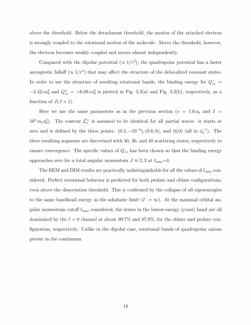
above the threshold. Below the detachment threshold, the motion of the attached electron
is strongly coupled to the rotational motion of the molecule. Above the threshold, however,
the electron becomes weakly coupled and moves almost independently.
Compared with the dipolar potential (∝ 1/r2), the quadrupolar potential has a faster
asymptotic falloff (∝ 1/r3) that may affect the structure of the delocalized resonant states.
In order to see the structure of resulting rotational bands, the binding energy for Q−zz =
−2.42 ea20 and Q+zz = +6.88 ea20 is plotted in Fig. 3.3(a) and Fig. 3.3(b), respectively, as a
function of J(J + 1).
Here we use the same parameters as in the previous section (s = 1.6 a0 and I =
104mea20). The contour L+
c is assumed to be identical for all partial waves: it starts at
zero and is defined by the three points: (0.3,−10−5), (0.6, 0), and (6,0) (all in a−10 ). The
three resulting segments are discretized with 30, 30, and 40 scattering states, respectively to
ensure convergence. The specific values of Qzz has been chosen so that the binding energy
approaches zero for a total angular momentum J ≈ 2, 3 at `max=4.
The BEM and DIM results are practically indistinguishable for all the values of `max con-
sidered. Perfect rotational behavior is predicted for both prolate and oblate configurations,
even above the dissociation threshold. This is confirmed by the collapse of all eigenenergies
to the same bandhead energy in the adiabatic limit (I → ∞). At the maximal orbital an-
gular momentum cutoff `max considered, the states in the lowest-energy (yrast) band are all
dominated by the ` = 0 channel at about 99.7% and 87.9%, for the oblate and prolate con-
figuration, respectively. Unlike in the dipolar case, rotational bands of quadrupolar anions
persist in the continuum.
18

3.3 Results for anions bounded by multipolar Gaussian
potentials
In this section, we investigate the generic near-threshold behavior of multipole-bound anions
at the transition between the subcritical (below dissociation threshold) and supercritical
(above dissociation threshold) regimes. The main objective of this part is to show the role
of low-` partial waves in shaping the properties of low-lying states. We assume that the
molecular potential has a Gaussian form given by Eq. (3.4). However, we wish to emphasize
that the particular choice of the radial form factor is not important as it represents an a priori
unknown short-range behavior. One can view this particular realization as a regularized zero-
range interaction. To study the threshold behavior of the system we investigate the pattern
of resonant poles as a function of four parameters: the strength and range of the Gaussian
form factor, the multipolarity of the potential, and the molecular moment of inertia.
19

3.3.1 Threshold trajectories for multipolar Gaussian potentials in
the adiabatic limit
0.0 0.2 0.4 0.6 0.8 1.0Potential range r0 (units of a0)
0.0
0.2
0.4
0.6
0.8
1.0
Pot
enti
alst
rengt
hV
0(R
y)
-4
-2
0
λ = 1
(a)
unbo
und
-8
-4
0
λ = 2
(b)
unbo
und
1 3 5
-12
-6
0
λ = 3
(c)
unbo
und
1 3 5-24
-12
0
λ = 4
(d)un
boun
d
V +0
−V −0
Figure 3.4: Threshold trajectories (V0, r0)±c for multipolar Gaussian potentials with λ = 1−4
in the adiabatic limit. Taken from Ref. [5].
As mentioned earlier, the critical multipole moments Q±λ,c mark the limit between the sub-
critical and supercritical regimes. One may notice that Q−λ,c = −Q+λ,c for odd-multipolarity
potentials, but there is no such relation for even multipolarity potentials. As discussed ear-
lier, there are two critical values of the quadrupole moment for a quadrupole-bound anion
(λ = 2): Q+2,c (prolate) and Q−2,c (oblate), and Q−2,c 6= −Q+
2,c.
As the usual −1/rλ+1 radial dependence of multipolar potentials is replaced in our work
20

by the Gaussian form factor, the dissociation threshold is obtained at the critical trajectories
of (V0, r0)±c . Fig. 3.4 shows such trajectories obtained in the adiabatic limit for the Jπ = 0+
1
g.s. of anions with multipolarities λ = 1− 4.
These results are obtained with a Berggren contour defined by the points kpeak =
(0.5,−0.1), kmid = 1.0, and kmax = 14.0 (in units of a−10 ), with each segment being discretized
by 40 Gauss-Legendre points. To ensure convergence, we took `max = 4 for λ = 1, 2, 3 and
`max = 8 for λ = 4, 5.
As one would expect, the absolute value of the critical potential strength |V0,c| required
to bind an excess electron decreases with the range r0 and for a fixed range |V0,c| increases
with multipolarity. Also, as noted in previous studies [7, 83, 88, 89], for even multipolarities,
the value of |V0,c| for negative-V0 potentials (“prolate”) is larger than that for positive-V0
potentials (“oblate”).
It is interesting to note that at the threshold the wave functions are dominated by the
` = 0 component. Dividing the intrinsic wave function into the inner region (r < R) and
outer region (r > R) contributions, where R is the distance at which the molecule potential
becomes practically unimportant, one can show [90, 91, 92] that the probability of finding
the electron in the outer region approaches one at the dissociation threshold if the ` = 0
component is present in the intrinsic wave function. This has been practically demonstrated
in our work on quadrupole-bound anions [7] in the context of the scaling properties of root-
mean-square (rms) radii.
3.3.2 Resonances of the near-critical quadrupolar Gaussian po-
tential
In order to study the role of low-` partial waves on the structure of multipole-bound anions,
one has to recognize the impact of ` = 0 partial waves on resonant states near threshold [92].
In our coupled-channel formalism, resonant states appear through the mixing of different
channels. To study general features of near-threshold resonances, we consider three states of
21

the quadrupolar potential in the adiabatic approximation. Namely, we investigate: (i) the
Jπ = 0+1 g.s. dominated by the ` = 0 partial wave; (ii) an excited Jπ = 0+
d state dominated
by the ` = 2 channel; and (iii) the lowest Jπ = 1−1 state, which is primarily ` = 1 and
without contribution from ` = 0. The quadrupolar case discussed here is characteristic of
other multipolar potentials.
(i) Resonant states dominated by the ` = 0 channel
The g.s. of the quadrupolar potential is computed with the BEM, using the extended contour
L+ defined by the points: k = (0, 0), (−0.1,−0.4), (0.1,−0.4), (2, 0), and (14, 0) (all in a−10 ),
each segment being discretized with 40 Gauss-Legendre points. By considering the contour
that extends into the third quadrant of the complex-momentum plane, antibound states can
be revealed [4, 93, 94].
22

0.0 0.2 0.4 0.6 0.8 1.0Potential strength V0 (Ry)
0.0
0.2
0.4
0.6
0.8
1.0
-0.1
0.0
0.1
Re(
E)
(Ry)
λ = 2 , Jπ = 0+1 , r0 = a0
(a)
Im(k)
Re(E)
7 8 9 10
0.0
0.4
0.8
1.2
Re(
Nl)
(b)
V0,c
� = 0
� = 2
� = 4
-0.4
0.0
0.4
Im(k
)(u
nits
ofa
−1
0)
Figure 3.5: The lowest 0+ resonant state of the quadrupolar Gaussian potential with r0 = a0as a function of V0. Top: real energy and imaginary momentum. Bottom: the channeldecomposition of the real part of the norm Re(N`). The critical strength V0,c is marked byarrow. Taken from Ref. [5].
Fig. 3.5(a) shows the energy and momentum of the 0+1 state for different values of the
potential strength V0. For large values of V0, the g.s. is bound (Re(E)<0) and has a positive
imaginary momentum. As the potential strength decreases, the energy of the g.s. moves
up and approaches the E = 0 threshold at V0,c = 8.7 Ry. For V0 < V0,c the lowest 0+ state
becomes antibound (Re(E) < 0, Im(k) < 0). With the complex-energy scheme, the norm
for the wave function also has a complex form. In our work, the sum of the real part of the
norm for all channels is normalized to 1. The real part of the norm for each channel can
have values beyond the range of 0 to 1. As illustrated in Fig. 3.5(b), the contributions N` to
23

the complex norm of the wave function from different `-channels (` = 0, 2, 4) vary smoothly
when crossing the threshold. The norm is largely dominated by the ` = 0 component. At
the critical strength, the ` > 0 contributions to the norm vanish, cf. discussion in Sec. 3.3.1.
This indicates that the presence of near-threshold antibound states indeed impacts the near-
threshold structure of weakly-bound systems [95, 96, 97, 98, 35].
(ii) Resonant states dominated by a ` 6= 0 channel
We now consider the evolution of an excited state of a wider quadrupolar potential with
r0 = 4 a0. At V0 =1.1 Ry, the lowest 0+ state is bound and the second Jπ = 0+2 state is
a decaying resonance, see Fig. 3.6. Figure 3.7(a) shows the channel decomposition for this
second 0+2 state. It is seen that its configuration has the predominant ` = 2 component.
24

1.00.0 0.1 0.2 0.3 0.4-0.4
-0.3
-0.2
-0.1
0.0
0+2
0+b
0+c
1.1 Ry
V0
2.7 Ry1.8 Ry
2.857 Ry
= 2, r0 = 4a
0+d
Re(k) (units of a−10 )
Im(k
)(u
nits
ofa
−1
0)
Figure 3.6: Trajectory of the 0+ resonant state in the complex-k plane of the quadrupolarpotential with r0 = 4 a0 as the potential strength V0 increases in the direction indicated byan arrow. At the lowest value V0 =1.1 Ry, the 0+ g.s. is bound and the state of interest is anexcited 0+
2 state associated with a decaying resonance. At V0 = 1.8 Ry the pole crosses the−45◦ line and becomes a subthreshold resonance 0+
d ≡ 0+2 . At V0 = 2.857 Ry the decaying
pole reaches the imaginary-k axis and coalesces with the capturing pole with Im(k) < 0forming an exceptional point. The antibound states at V0 = 1.8 Ry and V0 = 2.7 Ry aremarked. Taken from Ref. [5].
As the potential gets deeper, the pole crosses the −45◦ line at V0 ≈ 1.8 Ry and becomes
a subthreshold resonance labeled as 0+d . At V0 = 2.7 Ry, a rapid transition to a configuration
dominated by the ` = 4 partial wave takes place, which is indicative of a level crossing in the
25

complex-k plane. At V0 = 2.857 Ry the decaying pole arrives at the imaginary-k axis and
coalesces with the symmetric capturing pole forming an exceptional point [99, 100, 101]. At
still larger values of V0, the exceptional point splits up into two antibound states moving up
and down along the imaginary-k axis as shown in Fig. 3.6. A similar situation was discussed
in Refs. [43, 102] in the context of electron-molecule scattering and optical lattice arrays,
respectively.
0.0 1.0
-0.5
0.0
0.5
1.0
1.5
Re(
N�)
λ = 2
�= 0
�= 2
�= 4
Jπ
= 0+
1.0 1.5 2.0 2.5 3.0V0 (Ry)
-0.5
0.0
0.5
1.0
Re(
N�)
0+b 0+
c
1.8 2.7
0+d0+
(a)
(b) (c)
�= 2�= 2
�= 0
�= 0
�= 4 �= 4
Figure 3.7: Real norms of the channel wave functions for the decaying pole 0+d shown in
Fig. 3.6 and the antibound states 0+b and 0+
c of Fig. 3.8. Taken from Ref. [5].
In the range of V0 corresponding to the trajectory 0+2 → 0+
d shown in Fig. 3.6, there
26

appear antibound states in the threshold region. Their trajectories along the imaginary-k
axis are shown in Fig. 3.8 and their channel decompositions are given in Fig. 3.7(b) and
(c). As V0 increases, the antibound states 0+a , 0+
b , and 0+c emerge as bound physical states
of the system labeled as 0+1 , 0+
2 , and 0+3 , respectively. The lowest antibound state 0+
a has
a dominant ` = 0 configuration, similar to that of Fig. 3.5. At low values of V0, the wave
function of the antibound state 0+b is predominantly ` = 2. As seen in Fig. 3.6, this state
appears close to the decaying pole 0+d at V0 ≈ 1.8 Ry and the crossing between these two
poles in the complex-k plane is seen in their wave function decompositions. Following the
crossing, the state 0+b acquires a large ` = 0 component. The antibound state 0+
c begins as
an ` = 4 configuration. At V0 ≈ 2.7 Ry, this state interacts with 0+d and its configuration
changes to ` = 2. One can thus see that the presence of antibound states results in the
particular shape of the 0+d -pole trajectory in the complex-k plane.
27

0.0 0.2 0.4 0.6 0.8 1.00.0
0.2
0.4
0.6
0.8
1.0
0 1 2 3 4Potential strength V0 (Ry)
-0.4
-0.2
0.0
0.2
0.4
Im(k
)(u
nit
sof
a−
10
)λ = 2 r0 = 4 a0
0+1 0+
2 0+3
0+a
0+b
0+c
0+d
1.8
2.7
2.85
7
Figure 3.8: Trajectories of antibound and bound 0+ states along the imaginary-k axis asa function of V0 for the quadrupolar potential with r0 = 4 a0. With increasing potentialstrength, the antibound states 0+
a , 0+b , and 0+
c become bound states of the system 0+1 , 0+
2 ,and 0+
3 , respectively. The open circle marks the exceptional point of Fig. 3.6, which is thesource of two antibound states. The particular values of V0 discussed around Fig. 3.6 aremarked. Taken from Ref. [5].
28

0.0 0.2 0.4 0.6 0.8 1.00.0
0.2
1.0
0.0 0.2 0.4 0.6Re(k) (units of a−1
0 )
-0.6
-0.4
-0.2
0.0Im
(k)
(unit
sof
a−
10
)
λ = 2, Jπ = 0+d
r0 = 4 a0
r0 = 3 a0
r0 = 2 a0
r0 = 1.5 a0
r0 = a0
Figure 3.9: Trajectory of the 0+d resonant state in the complex-k plane for different values
r0 of quadrupolar potential as indicated by numbers (in units of a0). The ranges of V0 (inRy) are: (25.6-29.0) for r0 = a0; (9.7-14.5) for r0 = 1.5 a0; (4.8-10) for r0 = 2 a0; (1.7-4.79)for r0 = 3 a0; and (1.1-2.85) for r0 = 4 a0. Taken from Ref. [5].
The dependence of the 0+d -pole trajectory on the potential range is illustrated in Fig. 3.9.
For potentials with longer ranges, pole trajectories appear closer to the origin. Due to
the numerical stability issue, the contour used can not go below −0.4 a−10 for imaginary
momentum. Consequently, a wider potential with r0 = 4 a0 is chosen so that the whole
complex-momentum trajectory can be revealed. In all the cases shown, a transition from
decaying to subthreshold resonances takes place. These poles have large widths and are
expected to impact the structure of the low-energy scattering continuum.
29

(iii) Resonant states without a ` = 0 component
Here we discuss the lowest Jπ = 1−1 state, which is primarily ` = 1 with a small admixture of
the ` = 3 channel. This case closely follows the discussion of Ref. [43] for p-wave scattering
from short-range potentials.
0.0 0.2 0.4 0.6 0.8 1.00.0
0.2
0.4
0.6
0.8
1.0
-0.2 0.0 0.2 0.4 0.6Re(k) (a−1
0 )
-0.2
-0.1
0.0
0.1
0.2
λ = 2, Jπ = 1−1
r0 = a0
(a)
12.34
12.34
12.40
12.40
-0.05 0.00 0.05 0.10 0.15 0.20Re(E) (Ry)
0.00.20.40.60.81.0
Re(
N�)
(b)
� = 1
� = 3
Im(k
)(u
nit
sof
a−
10
)
Figure 3.10: Top: trajectory of the lowest 1−1 resonant state of the quadrupolar potential withr0 = a0 as a function of V0 in the range of (9-12.7) Ry. The potential strength V0 increasesalong the direction indicated by an arrow. The positions of the bound and antibound statesat V0 = 12.34 Ry and 12.4 Ry are marked. Bottom: real norms of channel functions for thisstate. Taken from Ref. [5].
The corresponding trajectory of this state in the complex-momentum plane is shown
30

in Fig. 3.10(a). At larger values of V0, the 1−1 state is bound. As V0 decreases, this state
crosses the dissociation threshold and becomes a narrow decaying resonance. The trajectory
of the capturing resonance, symmetric with respect to the imaginary-(k) axis, is not shown.
As discussed in Ref. [43], the exceptional point appears at the origin at V0,c. Close to the
threshold, the bound state and the antibound state are located symmetrically to the origin.
For the p-wave dominated state, the transition from the subcritical to the supercritical regime
is smooth, i.e., the wave function amplitudes hardly change with V0, see Fig. 3.10(b). This
is because the contributions from antibound and bound poles cancel each other out. In
this case, the structure of the low-energy continuum is not expected to be affected by the
presence of threshold poles.
The situation presented in Fig. 3.10 is rather generic for p-wave dominated resonant
poles. Increasing the potential range moves the pole trajectory closer to the real-k axis.
Consequently, states containing no s-wave component are likely to appear as isolated narrow
resonances. For odd-multipolarity potentials, a (j = J, ` = 0) component of a Jπ state
becomes large as the dissociation threshold is approached, see Sec. 3.3.2. On the other hand,
for even-multipolarity potentials, odd-J states cannot have an s-wave component, as the
molecule’s angular momentum j must be even, and narrow near-threshold resonances can
appear.
31

3.3.3 Rotational motion
3--0.02
-0.01
0.00
0.01
4+2+0+1- 5-
detachment threshold
angular momentum J
ener
gy (R
y)
λ = 1
Figure 3.11: The rotational band built upon the Jπ = 0+1 state of a dipole-bound anion. The
parameters V0 = 5.33 Ry, r0 = a0, and I = 103mea20 have been chosen to place the bandhead
energy slightly below the zero-energy threshold, where the rotational motion of the moleculecan excite the system into the continuum. The energy is plotted as a function of J(J + 1).Taken from Ref. [5].
To describe multipole-bound anions, one has to take into account the nonadiabatic coupling
between the rotational motion of the molecule and the s.p. motion of the electron. Whether a
multipole-bound anion can exhibit rotational bands depends on multipolarity. For instance,
it was shown in Ref. [58] that rotational bands of dipolar anions do not extend above the
dissociation threshold while a similar study for quadrupole-bound anions [7] demonstrated
that the rotational motion of the anion is hardly affected by the continuum.
32

-0.2
0.0
0.2
0.4
I = 50 mea20
I = 100mea20
angular momentum J
ener
gy (R
y)
3- 4+2+0+1- 5-
detachmentthreshold
λ = 2
Figure 3.12: Similar to Fig. 3.11 but for rotational bands built upon the Jπ = 0+1 and
1−1 bandheads of a quadrupolar Gaussian potential with V0 = 12.38 Ry, r0 = a0, and forI = 50mea
20 and I = 100mea
20. Taken from Ref. [5].
Figure 3.11 illustrates the case of a rotational band built upon the subthreshold Jπ = 0+1
state of the dipolar Gaussian potential. It is seen that the rotational band is not affected
when the zero-energy threshold is crossed below J = 4. In the realistic calculation for
dipole-boudn anions [58], it was found that rotational band does not extend beyond the
detachment threhshold, indicating a transition between strong-coupling regimes and weakly-
coupling regimes when cross the detachment threshold. Our result indicates that the presence
of the two coupling regimes predicted to exist in realistic calculations for dipole-bound an-
ions [58] must be due to difficulties in imposing proper boundary conditions at infinity for
the dipolar potential (∼ r−2) when the rotational motion of the molecule is considered nona-
diabatically [82]. Since in the present work the radial part of the dipolar pseudopotential is
replaced by a Gaussian function, the outgoing boundary condition can be readily imposed.
33

We now investigate the impact of the molecular rotation on the energy spectrum of the
anion. By definition, changing the moment of inertia of the molecule is expected to have
a larger effect on states dominated by channels with large j, but in practice, such channels
are unlikely to dominate at low energies. As an illustrative example, we study the 3−1 state
of the quadrupolar (λ = 2) Gaussian potential. Figure 3.13(a,b) shows, respectively, the
energy and decay width of the 3−1 resonance as a function of the potential strength and the
inverse moment of inertia.
A similar result is obtained for the quadrupolar case shown in Fig. 3.12 for two rotational
bands built upon the Jπ = 0+1 and 1−1 bandheads. The existence of rotational bands extend-
ing above the dissociation threshold is consistent with the findings of Ref. [7] employing the
realistic quadrupolar pseudopotential. The results for higher-multipolarity potentials follow
the pattern obtained for the dipolar and quadrupolar cases; hence, they are not shown here.
34

0.02
0.04 (a)
0.02
0.04
1/I(
units
of m
−1 ea−
2 0 )
(4,1)
(2,1)(b)
0.00.40.8
Re(N
)
(c) (4,1) (2,1)
1/I=0.04
8 10 12 14V0 (Ry)
0.00.40.8 (d)
1/I=0.02
0.0
0.4
0.8
E
Γ
E = 0
E = 0
Figure 3.13: Energy (a) and decay width (b), both in Ry, of the 3−1 resonance of the quadrupo-lar Gaussian potential with r0 = a0 as a function of the inverse of the moment of inertiaand the potential strength. The dissociation threshold (E = 0) is indicated. The dominant(j, `) channel is marked in panel (b). When the rotational energy of the molecule Ej=4
rot
lies below/above the energy of the 3−1 resonance, the (4,1) decay channel is open/closed.The line Ej=4
rot = E(3−1 ) (thick solid) separating these two regimes is marked, so is the lineEj=2
rot = E(3−1 ) (thick dotted) which corresponds to the threshold energy for the openingof the (2,1) channel. The norms of the two dominant channels (2,1) (solid line) and (4,1)(dotted line) are shown as a function of V0 for 1/I = 0.04m−1e a−20 (c) and 0.02m−1e a−20 (d).Taken from Ref. [5].
35

At large values of V0 when the 3−1 resonance lies close to the threshold, its wave function is
primarily described in terms of two channels with (j, `) = (2, 1) and (4, 1) with the dominant
(2,1) amplitude, see Fig. 3.13(c,d). At a finite value of I, as the energy of the resonance
increases, a transition takes place to a state dominated by the (4,1) component that is
associated with a reduction of the decay width. This transition can be explained in terms
of channel coupling. At very low values of 1/I, the energy E(3−1 ) lies above the rotational
4+ state of the molecule. As the moment of inertia decreases, the 4+ member of the g.s.
rotational band of the molecule moves up in energy, and at some value of I it becomes
degenerate with the energy of the E(3−1 ) resonance, i.e., Ej=4rot = E(3−1 ). At still higher
values of 1/I, the (4,1) channel is closed to the electron emission. As seen in Fig. 3.13(b),
the irregular behavior in the width of the resonance can be attributed to the (4,1) channel
closing effect [103]. A second irregularity in Fig. 3.13(c,d), seen at large potential strengths,
corresponds to Ej=2rot = E(3−1 ). As the resonance approaches the threshold, its tiny decay
width can be associated with the (0,3) channel. Due to its higher centrifugal barrier, (0,3)
channel contributes around 1% to the total norm in the threshold region.
3.4 Summary
In the chapter, two types of molecular anions approximated by a nonadiabatic electon-
plus-molecule model were studied using the complex-energy BEM within the coupld-channel
formalism, including both quadrupole-bound anions and anions bounded by multipolar Gaus-
sian potentials.
In the qudrupole-bound anions, the quadrupolar potential was generated by a linear
distribution of point charges, where the critical quadrupole moments calculated using both
BEM and DIM are compared with the analytical results. Rotational band for quadrupolar
anions were also predicted to extend above the detachment threshold.
Anions bounded by a multipolar Gaussian potential are expected to describe general
36

trends of near-threshold resonant poles for multipolarities λ ≥ 2. By calculating the thresh-
old lines for anions of different multipolarity, we predicted that within this model, higher-λ
anions can exist as marginally-bound open systems. The role of the low-` channels in shap-
ing the transition between subcritical and supercritical regimes has been explored. We
demonstrate the presence of a complex interplay between bound states, antibound states,
subthreshold resonances, and decaying resonances as the strength of the Gaussian potential
is varied. In some cases, we predict the presence of exceptional points. The fact that anti-
bound states and subthreshold resonances can be present in multipolar anions is of interest as
they can affect scattering cross sections at low energy. For Gaussian potentials, the outgoing
boundary condition can be readily imposed. Consequently, the rotational band of the anion
is not affected when the zero-energy threshold is reached. This indicates that the presence of
two coupling regimes of rotation predicted to exist in realistic calculations for dipole-bound
anions [58] must be due to specific asymptotic behavior of the dipolar pseudo-potential in the
presence of molecular rotation. The non-adiabatic coupling due to the collective rotation of
the molecular core can give rise to a transition into the supercritical region. We also predict
interesting channel-coupling effects resulting in variation of an anion’s decay width due to
rotation.
In summary, by looking systematically at the pattern of resonant poles of multipole-
bound anions near the electron detachment threshold we uncover a rich structure of the
low-energy continuum. These simple systems are indeed splendid laboratories of generic
phenomena found in marginally-bound molecules and atomic nuclei. It’s also noted our work
has promoted some experimental explorations of dipolar and quadrupolar anions [104, 105].
Besides providing guidance for experimental searching for the weakly bound anions, the study
on the generic properties of resonant states near the threshold can also help understand OQSs
in different areas.
37

Chapter 4
Lithium isotopes and mirror nuclei
4.1 Introduction
In the light-nuclei region of the nuclear landscape, the imbalance between proton and neu-
tron numbers can reach high values, which is susceptible to continuum effects due to the
presence of low-lying decay channels. Wave functions of such systems often “align” with the
nearby threshold and are expected to have substantial overlaps with the corresponding decay
channels. Among them, lithium isotopes are of particular interest as they reveal rich phe-
nomena, including the binary cluster (α+d) of 6Li [106, 107], the anitbound (virtual) state
of 10Li [44, 45, 46, 47], as well as the spatially extended halo structure of 11Li [18, 25, 108].
However, such OQSs pose many challenges for nuclear theory, since drip line nuclei can
not be described in a typical HO-based configuration interaction method. As a result, for
instance, the theoretical descriptions of 11Li are usually based on a few-body approximation,
including Faddeev equation [109] and other similar techniques [110, 111, 112, 113]. In this
case, 11Li is described as a loosely bound three-body system (9Li core and two valence
neutrons), due to its Borromean property [18, 25, 108], in which none of the two-body
subsystems is bound.
However, the core polarization effects can be large for some nuclei, where a cluster
approximation might not be sufficient, therefore, a more elaborated approach is required.
To this end, we adopt GSM based on the BEM technique introduced in Chapters 2 and 3,
which can give a comprehensive description of the interplay between many-body correlation
and continuum coupling.
38

In this work, we study the lithium isotopes (6−11Li) with a realistic residual interaction
including uncertainty estimation of the Hamiltonian parameters as well as predicted spectra.
Another interesting aspect existing only in nuclear OQSs is the asymmetry between
proton and neutron thresholds. This can result in different asymptotic behavior of proton
and neutron wave functions resulting in the Thomas-Ehrman effect (TEE) [114, 115]. To
study the TEE, the mirror partner of lithium isotopes have also been studied in this work.
4.2 Gamow shell model
4.2.1 Hamiltonian
The lithium isotopes and their mirror partners are studied in terms of valence nucleons
coupled to the 4He core. This is justified by the strongly bound nature of 4He, whose first
excited state is 20.21 MeV above the g.s. [1]. In this picture, the Hamiltonian is given as a
sum of an s.p. core-nucleon potential and effective two-body interactions among the valence
nucleons. In the intrinsic frame of the Cluster Orbital Shell Model (COSM) [116], where
the nucleon coordinates are defined with respect to the center of mass of the core, the GSM
Hamiltonian is expressed as:
H =n∑i
[p2i2µi
+ Ucore(i)
]+
n∑i=1,i<j
[Vi,j +
pipjMcore
](4.1)
where n denotes number of valence nucleons, µi and Mcore are the reduced mass of valence
nucleon and core, respectively, and Ucore, Vi,j are the core-nucleon potential and nucleon-
nucleon interaction, respectively. The last term in Eq. (4.1) is the recoil term in the COSM
coordinates, which is used to eliminate the energy contribution from the center-of-mass
motion. In GSM, to account for the many-body correlations, Slater determinants are built
upon the discretized s.p. Berggren basis states of each shell to serve as the many-body basis
within which the complex-symmetric H is diagonalized [4].
39

Core potential
The core-nucleon potential is taken as a Woods-Saxon (WS) field, with a central and spin-
orbit term and Coulomb field for protons.
Ucore(r) = V0f(r)− 4V`s1
r
df(r)
dr` · s+ UCoul(r), (4.2)
where f(r) = −(1 + exp[(r − R0)/a])−1. The WS radius and diffuseness parameters were
taken from Ref. [117]: R0(n) = 2.15 fm, R0(p) = 2.06 fm, a(n) = 0.63 fm, and a(p) = 0.64
fm. The Coulomb potential is generated by a spherical Gaussian charge distribution with
the radius Rch = 1.681 fm [118]. The strength of the central and the spin-orbit part of the
potential, represented as V0 and V`s, respectively, are optimized in the work with respect to
the selected states.
Two-body interaction
The effective two-body interaction is constructed based on the finite-range Furutani-Horiuchi-
Tamagaki (FHT) force [117, 119, 120], which has been shown to successfully describe struc-
ture and reactions involving light nuclei [121, 117, 122, 123, 124].
The FHT interaction contains central (c), spin-orbit (LS), tensor (T ) and Coulomb
terms:
V = Vc + VLS + VT + VCoul. (4.3)
The central and tensor parts are both a sum of three Gaussian functions with different
ranges representing the short, intermediate and long ranges of nucleon-nucleon interaction.
The spin-orbit part is a sum of two Gaussian functions [117]. In order to be applied in the
present GSM formalism, the interaction is rewritten in terms of the spin-isospin projectors
40

ΠST :
Vc(r) =V 11c f 11
c (r)Π11 + V 10c f 10
c (r)Π10
+ V 00c f 00
c (r)Π00 + V 01c f 01
c (r)Π01,
(4.4)
VLS = (L · S)V 11LSf
11LS(r)Π11, (4.5)
VT (r) = Sij[V11T f 11
T (r)Π11 + V 10T f 10
T (r)Π10], (4.6)
with the seven interaction strengths V STη (η = c, LS, T ) in different spin-isospin channels,
remaining to be adjusted to experimental data and fSTη are the unitless form factors [117].
r ≡ rij stands for the distance between the nucleon i and j, r = rij/rij, L is the relative
orbital angular momentum, S = (σi + σj)/2, and Sij = 3(σi · r)(σj · r)− σi · σj.
In Ref. [117], the FHT interaction was used in the GSM description of bound and
unbound nuclei with A ≤ 9. While a good energy reproduction was achieved, the systematic
statistical study of the parameters carried out in Ref. [117] demonstrated that some of the
terms in the FHT interaction were sloppy, i.e., not well constrained. According to this, we
used a simplified version of the FHT interaction where the central V 10c , V 01
c , and tensor
V 10T terms have been considered. This choice is also justified by the Effective Field Theory
(EFT) arguments [125, 126, 127, 128, 129]. Indeed, in the EFT expansion of the bare
nucleon-nucleon interaction, these three terms appear at leading order, whereas the other
terms present in the original FHT interaction correspond to higher orders of EFT. However,
we have observed that adding the central term V 00c improves the overall description of the
nuclei considered in this work and hence we have also included it in Vi,j.
As it is customary in shell model studies [130, 131], a mass-dependent interaction-scaling
factor of the form (6/A)α is introduced for the two-body interaction to effectively account
for the missing three-body forces [132, 133], where the factor is multiplied to all the two-
body interaction terms in Eq. 4.3. We found that the value α = 1/3 gives a very reasonable
description of experimental energies.
41

Finally, the Coulomb interaction between valence protons is treated by incorporating its
long-range part into the basis potential and expanding the short-range two-body component
in a truncated basis of HO states [134, 135].
4.2.2 Interaction optimization
In order to provide predictions, the interaction parameters have been optimized through a
fitting process, which consists in the minimization of the χ2 penalty function
χ2(p) =
Nd∑i=1
(Oi(p)−Oexpi
δOi
)2
, (4.7)
where Nd is the number of observables and p is a vector of parameter used. O(p) and Oexpi
are the calculated value for observables and experimental values, respectively. δOi is the
adopted error that has been estimated by normalizing the penalty function to the number
of degrees of freedom Ndof = Nd −Np at the minimum χ2(p0) [136]. In the case of a single
type of data and assuming that experimental and numerical errors are negligible, this can be
achieved through a global scaling of the initial adopted errors δOi → δOi√χ2(p0)/Ndof [117].
This renormalization guarantees that χ2 ∼ 1, which is necessary for calculated statistical
uncertainties to be meaningful [137].
Interactions used in this model are linear in strength parameters, which enables us to
calculate the first derivative (Jacobian J) exactly using Hellmann-Feynman theorem [138],
Jiα =1
δOi∂Oi∂pα
∣∣∣∣p0
. (4.8)
The covariance matrix C can be approximately expressed in terms of Jacobian J :
C ' (JTJ)−1 (4.9)
The uncertainty for each parameter is given by the diagonal elements in the covariance
42

matrix C, and the correlation between parameters α and β is given by [117]
cαβ =Cαβ√CααCββ
. (4.10)
In the situation where the Jacobian matrix is noninvertible or has a very small deter-
minant, the Gauss-Newton method used in the minimization of χ2 becomes unstable as the
Jacobian matrix must be inverted. This typically happens when some parameters are sloppy,
i.e., not well constrained by observables. To stabilize the calculation, the matrix inversion is
replaced by its pseudo-inverse, derived from the singular value decomposition (SVD) of the
Jacobian matrix [117].
Only well-established states are used for interaction optimization to give a solid basis
for this work, where both bound states and weakly bound states are both included. Weakly
bound states, such as g.s. of 11Li, are included so that the optimized interaction can be used
for extrapolation of states where continuum coupling is important.
The previous work [117] provides a good starting point for the core potentials and two
body interactions, which are fitted to the nucleon-4He phase shifts and selected states of
nuclei with mass number A ≤ 9, respectively. Only four parameters of two-body interaction
were well-constrained through statistical analysis and thus adopted in this work. An addi-
tional tuning of four strengths of the core potential was found to improve the optimization
quality further.
In this work, four strengths of the WS potential and four parameters of the two-body
interaction are thus simultaneously optimized to reproduce fifteen energy levels of lithium
isotopes and their mirror partners.
4.2.3 Model space
The calculations were performed in a model space which includes s1/2, p3/2 and p1/2 partial
waves for both protons and neutrons. Since the optimization involved energies only, for the
43

sake of speeding-up the optimization and for better stability, we used a deeper WS potential
to generate the basis, in which the 0p3/2 and 0p1/2 poles are bound. A real contour was
then used to describe the non-resonant continuum space. The contour L+ for Berggren
basis was divided into 3 segments with kpeak = 0.25 fm−1, kmid = 0.5 fm−1, and the cutoff
momentum kmax = 4 fm−1. Discretizing each segment with 10 points using the Gauss-
Legendre quadrature guaranteed the convergence of results.
To calculate resonance’s width, one has to generate a basis based on a much shallower
basis-generating WS potential, in which the 0p3/2 and 0p1/2 poles are decaying resonances.
In this case, a complex contour defined by a complex value of kpeak is employed. It is
to be noted that the calculation of the width is more demanding than that of energy. A
higher discretization of (20,20,20) is needed for the contour. Due to the Coulomb repulsion,
the mean-field used to generate the s.p. basis for proton-rich nuclei varies with proton
number. The contour was adjusted separately for each system to assure that the Berggren
completeness relation is met. To ensure the numerical stability, the chosen contour should
neither lie too close to the Gamow poles nor lie too far from the real-k axis. In this work,
kpeak is chosen to lie slightly (0.05 fm−1) below the position of the 0p3/2, 0p1/2 poles, but with
the imaginary part greater than −0.2 fm−1. The calculations were repeated with several
slightly different values of kpeak to assure the full convergence of results.
As in any configuration interaction models, the dimension of the Hamiltonian matrix
grows quickly with the number of active particles. In the context of the GSM, it increases
more quickly than in the conventional shell model due to the presence of discretized scat-
tering states. A more adapted basis is thus needed. The natural orbitals are defined as
the eigenvectors of the one-body density matrix [139], and have widely used in no-core shell
model [140]. In this work, we truncated the model space by working with natural orbitals
which provides an optimized set of s.p. states [117, 141, 139]. Natural orbitals are first
calculated in a truncated configuration space which permits only three valence particles in
the continuum shells. A truncation is then performed on the s.p. basis by keeping only
44

natural orbitals for which the modulus of the occupation number is greater than a certain
value (10−6). Finally, a new set of Slater determinants was constructed and served as the
basis for the diagonalization of the Hamiltonian matrix using the Davidson method [142].
To check the accuracy of this truncation procedure in the case of the largest systems,
computation of the energy was also performed using the Density Matrix Renormalization
Group (DMRG) method [143, 144]. The DMRG allows performing calculations without
truncation on the s.p. basis and without restrictions on the number of particles in the
continuum. In this approach, the many-body Schrodinger equation was solved iteratively in
tractable truncated spaces which were increased until numerical convergence was reached.
We have checked that, in all cases discussed in this work, the GSM results were in good
agreement with those of DMRG.
4.3 Results
4.3.1 Optimized states
To optimize our interaction, we used experimentally well-established levels, shown in Ta-
ble 4.1 and marked with F in Figs. 4.1 and 4.2 respectively. The experimental data are
taken from Ref. [1] unless otherwise specified. All energies are considered relative to the g.s.
energy of 4He.
As can be seen in Table 4.1, very good consistency with experimental results has been
achieved for the fifteen selected states. The rms deviation from experimental values is
160 keV. The largest discrepancy is obtained for the 1/2− states of 7Li and 7Be, with a
deviation of 340 keV from the data. All other states are within the range of 170 keV from
experiment.
We also want to point out that three states lying close to the threshold are also well re-
produced, including: (i) the 0+ state of 6Li which is 140 keV below the threshold of 4He+n+p;
(ii) the g.s. of halo nucleus 11Li lying 369 keV below the two-neutron emission threshold;
45

Table 4.1: Energy levels used in the GSM Hamiltonian optimization. The energies are givenwith respect to the 4He g.s.. The experimental values Eexp are taken from Ref. [1]. They arecompared to the GSM values EGSM.
Nucleus State Eexp (MeV) EGSM (MeV) Nucleus State Eexp (MeV) EGSM (MeV)6Li 1+ -3.70 -3.72
0+ -0.14 -0.107Li 3/2- -10.95 -11.02 7Be 3/2- -9.30 -9.36
1/2- -10.47 -10.14 1/2- -8.88 -8.538Li 2+ -12.98 -13.14 8B 2+ -9.44 -9.60
1+ -12.00 -11.93 1+ -8.67 -8.509Li 3/2- -17.05 -16.90 9C 3/2- -10.74 -10.85
1/2- -14.35 -14.50 1/2- -8.52 -8.5911Li 3/2- -17.41 -17.48
(iii) and the 2+ state of 8B being 140 keV away from one proton decay.
4.3.2 Optimized Interaction
The optimized values of the parameters for the WS potentials and the two-body interaction
are displayed, along with their statistical uncertainties, in Tables 4.2 and 4.4, respectively.
As one can judge from the small parameter uncertainties in Tables 4.2 and 4.4, the GSM
Hamiltonian is rather well constrained. As expected, the central term V 00c has the largest
uncertainty of ∼12%.
Table 4.2: Central and spin-orbit strengths of the core-nucleon WS potential optimized inthis work. The statistical uncertainties are given in parentheses.
Parameter Neutrons ProtonsV0 (MeV) 39.5 (2) 42.1 (4)V`s (MeV·fm2) 10.7 (2) 11.1 (5)
Table 4.3: Groud state energies (in MeV) and widths (in keV) of 5He and 5Li obtained fromthe optimized core-nucleon potential and compared to experiments [2, 3].
Nucleus EGSM Eexp ΓGSM Γexp5He 0.74 0.798 640 6485Li 1.6 1.69 1300 1230
46

Table 4.4: Strengths V STη of the two-body interaction optimized in this work. The statistical
uncertainties are given in parentheses.
parameter valueV 01c (MeV) -9.425 (70)V 10c (MeV) -8.309 (90)V 00c (MeV) -8.895 (1130)
V 10T (MeV·fm−2) -22.418 (970)
Compared with the core-nucleon potential parameters obtained by fitting proton-4He
and neutron-4He phase shifts in Ref. [117], the strength parameter of core potentials for both
protons and neutrons are shallower, which push p-shell poles up further into the continuum.
Moreover, the spin-orbit strength is larger than that in Ref. [117], which separates the 0p3/2
and 0p1/2 poles further apart. Consequently, the 0p3/2 pole appears at similar energy as in
Ref. [117] and the 0p1/2 pole lies high above in the continuum. To assess the quality of the
newly obtained interaction, the energy and width for the g.s. (3/2−) of both 5He and 5Li are
calculated and shown in Table 4.3. These values are indeed very close to the experimental
values.
The new core potential is not optimal in describing 0p1/2 resonant states of 5He and 5Li,
whose physical importance decrease with its large decaying width. But this does not extend
to heavier nuclei. For example, the 1/2− state of 7Li and 7Be are mainly determined by the
0p1/2 pole and the obtained results are still quite close to the experimental data.
4.3.3 Test against other excited states
To check the quality of our optimized interaction, states not included in the optimization
were calculated and compared with experiment. Results are shown in Figs. 4.1 and 4.2. To
distinguish from the states used for optimization, states not entering the optimization are
shown together with their energies displayed; the widths are marked by the shaded boxes.
The corresponding energies and statistical uncertainties of predicted states are listed in
Table 4.5. As one can see, the optimized interaction not only allows for a good reproduction
47

0.0 0.2 0.4 0.6 0.8 1.00.0
0.2
0.4
0.6
0.8
1.0
6Li 7Li 8Li 9Li 10Li 11Li
−16
−14
−12
−10
−8
−6
−4
−2
0
2
En
ergy
(MeV
) 1+
3+
0+
2+2+
-1.57
1.78
2.23
-1.51
0.6
1.67
3/2−1/2−
7/2−
5/2−
5/2−
-6.04
-3.50
-1.73
-6.3
-4.34
-3.49
GSMexp
2+
1+
3+
1+
-10.59
-8.9
-10.73
-9.77
3/2−
1/2−
5/2−-12.64 -12.75
1+
2+
1−2−
-16.22
-16.55
-15.5
-16.78
-16.54
-15.55
3/2−
−16.5
−16.0 10Li
GSM
exp1999
exp2015
1+
2+
1+
2+1+
2+
Figure 4.1: Energies for states of Li isotopes with respect to 4He. Red lines denote GSMresults and the black lines mark experimental values. The shaded area represents the widthof the corresponding resonance. States used for optimization are marked with a F, theirenergies are listed in Tables 4.1 and 4.5.
48

of experimental energies for the fifteen selected states but also gives satisfactory results
for excited states not included in the fit. For instance, the calculated 3+ state in 6Li at
−1.57 MeV is only 60 keV below the experimental energy. The experimental widths for the
second 5/2− state in 7Li (89 keV) and 5/2− state in 9Li (88 keV) are very reasonable: the
calculated values are 22 and 62 keV, respectively.
The 5/2− and 7/2− excited states in 7Be are slightly (>300 keV) above the correspond-
ing experimental values, whereas the position of the 3+ state in 8B and 5/2− state in 9C
are well reproduced. It is also worth to mention that the second excited state 5/2− of 9C is
in good consistency with the R-matrix analysis and continuum shell model calculations in
Ref. [145]. The calculated width for 5/2− state is 340 keV and very close to the value 673 ±
50 keV extracted from experiment [146].
Table 4.5: Energy levels for states not entering the optimization. The experimental valuesEexp are taken from Ref. [1]. The GSM values EGSM are shown with the uncertainties inparentheses.
Nucleus State Eexp (MeV) EGSM (MeV) Nucleus State Eexp (MeV) EGSM (MeV)6Li 3+ -1.51 -1.57(2)7Li 7/2− -6.3 -6.04(2) 7Be 7/2− −4.73 −4.47(2)8Li 3+ -10.73 -10.59(2) 8B 3+ -7.12 -7.11(2)9Li 5/2− -12.75 -12.64(2) 9C 5/2− -7.14 -7.12(5)10Li 2+ -16.78 -16.55(5) 10N 1− -8.84 -8.93(6)
1+ -16.54 -16.22(5) 2− -7.94 -8.46(6)
In general, we do not expect the same quality of data reproduction for all excited states
due to the fact that the higher partial waves with ` ≥ 2, which may contribute to the wave
functions of those states, are not included in the model space. The estimated statistical
uncertainties on the predicted energies are small: in most cases they are in the range of 20
– 60 keV.
49

Table 4.6: Root-mean-square proton (Rp) and neutron (Rn) radii of 6Li, 7Li/7Be, 8Li/8B,9Li/9C, and 11Li (in fm).
Nucleus State Rp/Rn(fm) Nucleus State Rp/Rn(fm)6Li 1+ 2.22/2.217Li 3/2− 2.12/2.28 7Be 3/2− 2.26/2.098Li 2+ 2.12/2.48 8B 2+ 2.57/2.149Li 3/2− 2.12/2.53 9C 3/2− 2.62/2.0911Li 3/2− 2.12/2.81
4.3.4 Root-mean-square radius
One of the key features to identify halo nucleus is the rms radius. To give an estimation, Ta-
ble 4.6 shows rms proton/neutron radius for lithium isotopes and their mirror partners [147]:
< r2 >=2
Nval + 2< r2core > +
Nval
Nval + 2< r2i >, (4.11)
where the first and second term corresponds to the contribution from both the core and
valence particles, respectively, with Nval being the number of valence protons/neutrons. The
experimental value of 1.67 fm is used for the rms radius of both proton and neutron in the
4He core [148]. Valence protons and neutrons are treated as point-like particles, whose sizes
are not taken into account.
Since the corrections, such as spin-orbit effects and core swelling [147], are not included
in our calculation, we do not intend to compare our results directly against to the experi-
mental charge radii.
By comparing with other lithium isotopes, a dramatical increase of the rms neutron
radius of 11Li can be seen from Table 4.6, which indeed indicates the halo structure in 11Li.
Since all considered Li isotopes have only one well-bound valence proton, the proton radii
are almost constant for each Li isotopes.
As to the proton-rich side, a sharp increment can be seen clearly for the rms proton
radii for 8B and 9C as compared to those of 6Li and 7Be, suggesting that both 8B and 9C
50

0.0 0.2 0.4 0.6 0.8 1.00.0
0.2
0.4
0.6
0.8
1.0
7Be 8B 9C 10N 11O
−10
−8
−6
−4
−2E
ner
gy(M
eV)
3/2−
1/2−
7/2−
5/2−
-4.47
-2.3
-4.73
-2.57
2+
1+
3+ -7.11 -7.12
GSM exp
3/2−
1/2−
5/2−-7.12 -7.14
1−2−2+1+
-8.93
-8.46-8.12
-7.9
-8.84
-7.94
3/2−
5/2+
Figure 4.2: Similar to Fig. 4.1 for results of mirror nuclei of Li isotopes. Energies are givenwith respect to g.s. of 4He. Experimental energy of the 5/2− resonance in 9C was takenfrom Ref. [8] and the data for 11O is from Ref. [9].
are indeed good candidates for proton halo nuclei due to their weakly bound properties
[149, 150, 151].
4.3.5 Prediction for unbound nuclei: 10Li, 10N and 11O
10Li
Several experiments [44, 45, 46, 47] and theoretical calculations [152, 93] have indicated
that the structure of the g.s. in 10Li may correspond to a neutron in a virtual ` = 0 state
above a 9Li core. However, the presence of such a virtual state near the threshold has
not been confirmed in a recent experiment [153] with higher statistics, see the theoretical
analysis [154, 155]. This indicates that the situation in 10Li is still not well understood.
We wish to note, however, that a virtual state in 10Li cannot be associated with an
energy level of the system; the appearance of such a state in the complex-momentum plane
51

manifests itself through a low-energy enhancement of the n+9Li cross-section. For that
reason, we limited our calculations to resonant states in 10Li that can be interpreted as
experimentally-observable resonances.
The computed 2+ g.s. and first excited state 1+ of 10Li lie at 0.35 and 0.68 MeV above
the n+9Li threshold, respectively. The next excited states are the degenerate 1− and 2−
states at 1.05 MeV. Due to the strong coupling to the continuum in these states, using the
WS potential of the GSM Hamiltonian to generate the basis would make the numerical
computation unstable. To achieve the numerical stability, the computations were performed
by a deeper WS potential. We have checked that our predicted energies do not depend on the
choice of the WS used for the construction of the basis: in all cases considered, the variation
of the energy did not exceed 1 keV. On the other hand, the computed width associated with
the states is of the order of a few hundred keV and consequently not stable. For that reason,
we do not show them in Fig. 4.1.
To shed light on the structure of 10Li, Table 4.7 lists the squared amplitudes of the
dominant neutron configurations for the four low-lying states of 10Li. The positive parity
states are primarily made from the 0p3/2 and 0p1/2 resonant shells. The negative parity states
contain one neutron in the 1s1/2 shell. The contribution from the non-resonant continuum
space to the low-lying states is very small.
Experimentally, Ref. [156] observed two positive-parity states at 0.24 MeV and 0.53 MeV
above the n+9Li threshold [156], with the lower state assigned to be 1+. This spin assignment
contradicts the results in Ref. [157] where the lowest positive parity state was assigned to
be a 2+, see the inset in Fig. 4.1. In our prediction, the computed position of 1−, 2− are in
agreement with the observation of a negative-parity state at 1.05 MeV from Ref. [153].
Unbound 10N
10N is the unbound mirror partner of 10Li, lying beyond proton dripline. The spectrum of
10N is not experimentally known with certainty. In Fig. 4.2, we show the tentative level
52

Table 4.7: Squared amplitudes of dominant configuration of valence neutrons and protonsfor low-lying levels of 10Li and 10N, respectively. Energies with respect to the one-nucleonemission threshold are shown in the parentheses for each state. The odd proton in 10Li andthe odd neutron in 10N occupy the 0p3/2 Gamow state. The tilde sign labels non-resonantcontinuum components.
configuration 10Li 10N2+ (0.35 MeV) 1+ (0.68 MeV) 2+(2.73 MeV) 1+(2.95 MeV)
(0p3/2)4(0p1/2)
1 0.84 0.81 0.81 0.78(0p3/2)
3(0p1/2)2 0.10 0.06 0.10 0.05
1−(1.4 MeV) 2−(1.4 MeV) 1−(1.92 MeV) 2−(2.39 MeV)(0p3/2)
4(1s1/2)1 0.72 0.73 0.44 0.37
(0p3/2)4(s1/2)
1 0.29 0.35(0p3/2)
3(0p1/2)1(1s1/2)
1 0.14 0.14 0.09 0.07(0p3/2)
3(0p1/2)1(s1/2)
1 0.06 0.07(0p3/2)
2(0p1/2)2(1s1/2)
1 0.07 0.07 0.04 0.03(0p3/2)
2(0p1/2)2(s1/2)
1 0.03 0.03
assignments used in Ref. [1]. According to Refs. [158, 159], the g.s. of 10N is most likely a 1−
state in the energy range from 1.81 to 1.94 MeV. In a more recent work [160], they observed
two low-lying negative-parity states but they were not able to assign Jπ values.
Due to the presence of the Coulomb barrier, the 1s1/2 single-proton state is a broad
resonance rather than a virtual state [9, 161]. To capture this state, a complex contour is
used with kpeak = (0.25,−0.05) fm−1. Our calculations for 10N predict the g.s. to be a 1−
state with (E,Γ) = (−8.93, 0.9) MeV that lies 1.92 MeV above the 1p threshold. The first
excited state is predicted to be a 2− state with Γ = 0.3 MeV slightly below the value quoted
in Ref. [160]. This result is consistent with the recent Gamow coupled-channel analysis of
Ref. [161]. We also predict an excited 1+ state with Γ=0.3 MeV, lying 2.9 MeV above the
9C+p threshold, which is consistent with Refs. [162, 163, 164]. A second positive-parity state
with Jπ = 2+ is also predicted at 0.81 MeV with a width of 0.36 MeV.
Table 4.7 shows the squared amplitudes of the dominant proton configurations for the
four low-lying states of 10N. Similar to 10Li, the positive parity states are primarily made
from the 0p3/2 and 0p1/2 resonant shells. The dominant configurations of negative parity
states contain one ` = 0 proton, which can either be in the 1s1/2 shell or in a non-resonant
53

continuum state.
Unbound 11O
11O is a 2p-emitter as the mirror partner of the 2n-halo nucleus 11Li. With one more proton
above 10N, 11O is more unbound, which makes it more challenging to study experimentally.
The first observation of 11O was done recently with two-neutron knockout reactions of 13O
beams at NSCL [9]. A broad peak with a width of 3.4 MeV was observed which was inter-
preted in terms of four overlapping resonances:Jπ = 3/2−1 , 3/2−2 , 5/2
+1 , 5/2
+2 [9, 161]. The
3/2−1 and 5/2+1 states are 4.16 MeV and 4.65 MeV above 9C+2p threshold and the widths
are 1.3 MeV and 1.06 MeV respectively.
In this work, we predicted the g.s. 3/2−1 at 4.85 MeV with a width of 0.13 MeV and a
first excited state 5/2+1 at 5.03 MeV with the width of about 1 MeV. These predictions are
consistent with the Gamow coupled-channel calculations of Refs. [9, 161].
4.3.6 Continuum effects on the Thomas-Ehrman shift
The Thomas-Ehrman shift [114, 115] reflects the energy shift between the mirror pair of
nuclei primarily due to the Coulomb repulsion. To study the effect of particle continuum
due to different positions of particle thresholds in mirror partners, we compared the level
schemes of Li isotopes and their mirror partners with mass number A = 7, 8, 9, 10, from
well-bound states to unbound resonances high above the threshold. Results are shown in
Fig. 4.3. Within each pair, the ground states agree.
This agreement holds for excited states as long as both are bound, as can be seen for
the 3/2−,1/2− and 7/2− states of A = 7 nuclei in Fig. 4.3(a). Moving up to higher energy,
the 5/2− state of 7Li and 7Be are both above the one-nucleon emission threshold. The 5/2−
level of proton-rich nuclei 7Be is lower than that of the neutron-rich partner 7Li.
A similar trend can also be seen in results for the 8Li/8B and 9Li/9C pairs in Fig. 4.3(b,c).
As discussed in Sec. 4.3.4, 8B and 9C are both likely to be halo nuclei having large spatial
54

..
2
.
.
7Li 7Be0
2
4
6
3/ 2−1/ 2−
7/ 2−
5/ 2−6Li+n
6Li+p
8Li 8B0
1
2
2+
1+
3+
7Li+n
7Be+p
9Li 9C01234
3/ 2−
1/ 2−
5/ 2−
8Li+n
8B+p
10Li 10N-2
-1
0
12+1+
1− / 2−
1−2−2+1+
9Li+n
9C+p
(a) (b)
(c) (d)
Ene
rgy
(MeV
)
Figure 4.3: Spectrum for Li isotopes and their mirror partner with mass (a) A = 7, (b)A = 8, (c) A = 9, (d) A = 10. Within each pair, the spectrum of Li isotope and its mirrorare plotted whin the same scale and different range. The plots are shifted so that the g.s.of each pair align with each other. The one-proton/neutron emission thresholds are alsomarked within each plot.
55

extensions.
The 10Li/10N pair is the most interesting one as both nuclei lie above the particle
threshold. As seen in Table 4.7, the effect of the very low 9C+p threshold in 10N on the
negative-parity states 1− and 2− containing the s-wave proton is huge: it results in a rather
dramatic shift of both negative parity states when going from 10Li to 10N that gives rise to
a different structure of low-lying resonances in these nuclei.
56

Chapter 5
Conclusion and perspectives
This thesis is devoted to the study of OQSs with the complex-energy methods and proper
description of continuum coupling. By studying both atomic anions and lithium isotopes
(including their mirror partners), this work addresses important problems in the field of
OQSs in atomic physics and nuclear physics.
In the atomic domain, quadrupolar anions and anions bounded by the multipolar Gaus-
sian potentials were simulated using the complex-energy electron-plus-molecule model. The
coupling between the rotational motion of the molecule and the valence electron near the
dissociation threshold has been studied. By analyzing the rotational bands extended above
the dissociation threshold, we predicted that spatial charge distribution does not affect the
coupling between the molecule’s rotational motion and electron’s motion.
As for anions bounded by multipolar Gaussian potential, effects of the low-` channels
on the trajectory of resonant states in the complex-momentum plane are revealed. By
increasing potential strength, a resonance with a moderate contribution from s-wave can
become a subthreshold resonance, and then an antibound state that eventually becomes a
bound state. This demonstrates that antibound states and subthreshold resonances, which
can not be observed in experiments, can profoundly affect the structure of OQSs.
In the nuclear physics area, the properties of lithium isotopes and their mirror partners
have been studied with an optimized FHT interaction. This interaction has been devel-
oped by fitting energies to fifteen well-established states of lithium isotopes and their mirror
partners, with an rms deviation from experiments of 160 keV. Statistical analysis of the
interaction parameters indicates the statistical uncertainty less than 12%. Calculations for
57

other excited states demonstrate the good predictive power of the new interaction. Predic-
tions have been make for the spectra of very exotic nuclei 10Li, 10N and 11O. A very large
Thomas-Ehrmann effect has been predicted for 10Li/10N pair.
In summary, in this work, I applied the complex-energy method to study OQSs, from
the simple one-body system (atomic anions) to the complicated many-body systems (lithium
isotopes and their mirror partners). The success of depicting lithium isotopes highlights the
ability of GSM to describe both well-bound nuclei and exotic nuclei systematically. With
interactions extracted from well-bound systems and systems near the threshold, reliable
predictions can be made for exotic isotopes lying above the threshold. More solid and
insightful works are expected to help understand other exotic nuclei. One possibility for
future work is to extend this work to other isotopic chains such as boron and beryllium
isotopes. By extracting interaction information from well-established states of each isotopic
chain, extrapolations can be made for the more exotic boron and beryllium isotopes. Also,
since boron and beryllium isotopes have more valence protons than the lithium isotopes,
proton-neutron pairing is expected to play a more important role. By comparing different
interactions adapted to each isotopic chain, a better understanding of the interactions is
expected.
Besides 4He, other nuclei, such as 22O, can also serve as the core, with which heavier
isotopes like oxygen, fluorine isotopes are accessible. This work focused on the spectra of
the studied nuclei and also explored the size of halo nuclei. Other anticipated applications
include two-nucleon radioactivity, clustering, and isospin violation in dripline nuclei.
With the current high-performance computing facilities, this work was able to extend
calculations for a nucleus core with up to seven valence nucleons. Calculations with more
valence nucleons in a larger space are still inaccessible. Algorithms that can better take
advantage of the modern computational facilities, such as GPUs, are also expected to benefit
the understanding of OQSs.
58

APPENDIX
59

List of Publications
1. K. Fossez , X. Mao, W. Nazarewicz, N. Michel, W. R. Garrett, and M. P loszajczak.
Resonant spectra of quadrupolar anions. Phys. Rev. A, 94:032511, 2016. (discussed
in Chapter 3)
• Performed the calculation for rotational bands.
• Contributed to the rotational bands part of the draft.
2. X. Mao, K. Fossez, W. Nazarewicz. Resonant spectra of multipole-bound anions.
Phys. Rev. A, 98:062515, 2018.(discussed in Chapter 3)
• Developed a C++ code for the Gaussian potential part.
• Performed the calculations, analyzed results, and produced figures.
• Wrote the first draft of the manuscript.
3. X.Mao, J.Rotureau, W.Nazarewicz. Gamow shell model description of Li isotopes
and their mirror partners. arXiv:2004.02981, 2020. (discussed in Chapter 4)
• Carried out all the calculations, including the interaction optimization and GSM
studies of individual nuclei .
• Developed Python scripts to generate all the plots.
• Selected experimental data and researched literature.
• Wrote the first draft of the manuscript.
60

BIBILOGRAPHY
61

BIBLIOGRAPHY
[1] http://www.nndc.bnl.gov/ensdf, 2015.
[2] D. R. Tilley, C. M. Cheves, J. L. Godwin, G. M. Hale, H. M. Hofmann, J. H. Kelley,C. G. Sheu, and H. R. Weller. Energy levels of light nuclei A = 5, 6, 7. Nucl. Phys. A,708:3, 2002.
[3] http://www.tunl.duke.edu/nucldata/, 2015.
[4] N. Michel, W. Nazarewicz, M. P loszajczak, and T. Vertse. Shell model in the complexenergy plane. J. Phys. G, page 013101, 2009.
[5] X. Mao, K. Fossez, and W. Nazarewicz. Resonant spectra of multipole-bound anions.Phys. Rev. A, 98:062515, 2018.
[6] W. R. Garrett. Critical electron binding to linear electric quadrupole systems. J.Chem. Phys., 128:194309, 2008.
[7] K. Fossez, X. Mao, W. Nazarewicz, N. Michel, W. R. Garrett, and M. P loszajczak.Resonant spectra of quadrupolar anions. Phys. Rev. A, 94:032511, 2016.
[8] G. V. Rogachev, J. J. Kolata, A. S. Volya, F. D. Becchetti, Y. Chen, P. A. DeYoung,and J. Lupton. Spectroscopy of 9C via resonance scattering of protons on 8B. Phys.Rev. C, 75:014603, 2007.
[9] T. B. Webb, S. M. Wang, K. W. Brown, R. J. Charity, J. M. Elson, J. Barney, G. Cer-izza, Z. Chajecki, J. Estee, D. E. M. Hoff, S. A. Kuvin, W. G. Lynch, J. Manfredi,D. McNeel, P. Morfouace, W. Nazarewicz, C. D. Pruitt, C. Santamaria, J. Smith,L. G. Sobotka, S. Sweany, C. Y. Tsang, M. B. Tsang, A. H. Wuosmaa, Y. Zhang, andK. Zhu. First observation of unbound 11O, the mirror of the halo nucleus 11Li. Phys.Rev. Lett., 122:122501, 2019.
[10] T. Berggren. On the use of resonant states in eigenfunction expansions of scatteringand reaction amplitudes. Nucl. Phys. A, 109:265, 1968.
[11] T. Berggren and P. Lind. Resonant state expansion of the resolvent. Phys. Rev. C,47:768, 1993.
[12] A. B. Balantekin, J. Carlson, D. J. Dean, G. M. Fuller, R. J. Furnstahl, M. Hjorth-Jensen, R. V. F. Janssens, Bao-An Li, W. Nazarewicz, F. M. Nunes, and W. E. Or-mand. Mod. Phys. Lett. A, 29:1430010, 2014.
[13] J. Al-Khalili. An Introduction to Halo Nuclei. Springer Berlin Heidelberg, Berlin,Heidelberg, 2004.
[14] K. Riisager. Nuclear halo states. Rev. Mod. Phys., 66:1105, 1994.
62

[15] A. S. Jensen, K. Riisager, D. V. Fedorov, and E. Garrido. Structure and reactions ofquantum halos. Rev. Mod. Phys., 76:215, 2004.
[16] V. Tripathi, S. L. Tabor, P. F. Mantica, C. R. Hoffman, M. Wiedeking, A. D. Davies,S. N. Liddick, W. F. Mueller, T. Otsuka, A. Stolz, B. E. Tomlin, Y. Utsuno, andA. Volya. 29Na: Defining the edge of the island of inversion for Z = 11. Phys. Rev.Lett., 94:162501, 2005.
[17] Y. Kondo, T. Nakamura, R. Tanaka, R. Minakata, S. Ogoshi, N. A. Orr, N. L. Achouri,T. Aumann, H. Baba, F. Delaunay, P. Doomenbal, N. Fukuda, J. Gibelin, J. W. Hwang,N. Inabe, T. Isobe, D. Kameda, D. Kanno, S. Kim, N. Kobayashi, T. Kobayashi,T. Kubo, S. Leblond, J. Lee, F. M. Marques, T. Motobayashi, D. Murai, T. Murakami,K. Muto, T. Nakashima, N. Nakatsuka, A. Navin, S. Nishi, H. Otsu, H. Sato, Y. Satou,Y. Shimizu, H. Suzuki, K. Takahashi, H. Takeda, S. Takeuchi, Y. Togano, A. G. Tuff,M. Vandebrouck, and K. Yoneda. Nucleus 26O: A barely unbound system beyond thedrip line. Phys. Rev. Lett., 116:102503, 2016.
[18] J. S. Al-Khalili and J. A. Tostevin. Matter radii of light halo nuclei. Phys. Rev. Lett.,76:3903, 1996.
[19] M. Freer. The clustered nucleus–cluster structures in stable and unstable nuclei. Rep.Prog. Phys., 70:2149, 2007.
[20] M. Freer, H. Horiuchi, Y. Kanada-En’yo, D. Lee, and U. Meißner. Microscopic clus-tering in light nuclei. Rev. Mod. Phys., 90:035004, 2018.
[21] C. Dossat, A. Bey, B. Blank, G. Canchel, A. Fleury, J. Giovinazzo, I. Matea,F. de Oliveira Santos, G. Georgiev, S. Grevy, I. Stefan, J. C. Thomas, N. Adimi,C. Borcea, D. Cortina Gil, M. Caamano, M. Stanoiu, F. Aksouh, B. A. Brown, andL. V. Grigorenko. Two-proton radioactivity studies with 45Fe and 48Ni. Phys. Rev. C,72:054315, 2005.
[22] B. Blank, A. Bey, G. Canchel, C. Dossat, A. Fleury, J. Giovinazzo, I. Matea, N. Adimi,F. De Oliveira, I. Stefan, G. Georgiev, S. Grevy, J. C. Thomas, C. Borcea, D. Cortina,M. Caamano, M. Stanoiu, F. Aksouh, B. A. Brown, F. C. Barker, and W. A. Richter.First observation of 54Zn and its decay by two-proton emission. Phys. Rev. Lett.,94:232501, 2005.
[23] J. Giovinazzo, B. Blank, M. Chartier, S. Czajkowski, A. Fleury, M. J. Lopez Jimenez,M. S. Pravikoff, J.-C. Thomas, F. de Oliveira Santos, M. Lewitowicz, V. Maslov,M. Stanoiu, R. Grzywacz, M. Pfutzner, C. Borcea, and B. A. Brown. Two-protonradioactivity of 45Fe. Phys. Rev. Lett., 89:102501, 2002.
[24] B. Blank and M. P loszajczak. Two-proton radioactivity. Rep. Prog. Phys., 71:046301,2008.
[25] I. Tanihata, H. Hamagaki, O. Hashimoto, Y. Shida, N. Yoshikawa, K. Sugimoto, O. Ya-makawa, T. Kobayashi, and N. Takahashi. Measurements of interaction cross sectionsand nuclear radii in the light p-shell region. Phys. Rev. Lett., 55:2676, 1985.
63

[26] D. L. Auton. Direct reactions on 10Be. Nucl. Phys. A, 157:305, 1970.
[27] F. Ajzenberg-Selove, E. R. Flynn, and O. Hansen. (t, p) reactions on 4He, 6Li, 7Li,9Be, 10B, 11B, and 12C. Phys. Rev. C, 17:1283, 1978.
[28] R. Ringle, M. Brodeur, T. Brunner, S. Ettenauer, M. Smith, A. Lapierre, V.L. Ryjkov,P. Delheij, G.W.F. Drake, J. Lassen, D. Lunney, and J. Dilling. High-precision Penningtrap mass measurements of 9,10Be and the one-neutron halo nuclide 11be. Phys. Lett.B, 675(2):170, 2009.
[29] H. Esbensen, B. A. Brown, and H. Sagawa. Positive parity states in 11Be. Phys. Rev.C, 51:1274, 1995.
[30] M. V. Zhukov, B. V. Danilin, D. V. Fedorov, J. M. Bang, I. J. Thompson, and J. S.Vaagen. Bound state properties of Borromean halo nuclei: 6He and 11Li. Phys. Rep.,231:151, 1993.
[31] G. Gamow. Zur Quantentheorie des Atomkernes. Z. Physik, 51:204, 1928.
[32] R. W. Gurney and E. U. Condon. Quantum mechanics and radioactive disintegration.Phys. Rev., 33:127, 1929.
[33] A. F. J. Siegert. On the derivation of the dispersion formula for nuclear reactions.Phys. Rev., 56:750, 1939.
[34] L. P. Kok. Accurate determination of the ground-state level of the 2He nucleus. Phys.Rev. Lett., 45:427, 1980.
[35] A. M. Mukhamedzhanov, B. F. Irgaziev, V. Z. Goldberg, Yu. V. Orlov, and I. Qazi.Bound, virtual, and resonance S-matrix poles from the Schrodinger equation. Phys.Rev. C, 81:054314, 2010.
[36] A. M. Mukhamedzhanov, Shubhchintak, and C. A. Bertulani. Subthreshold resonancesand resonances in the R-matrix method for binary reactions and in the Tgrojan horsemethod. Phys. Rev. C, 96:024623, 2017.
[37] S. A. Sofianos, S. A. Rakityansky, and G. P. Vermaak. Subthreshold resonances infew-neutron systems. J. Phys. G, 23:1619, 1997.
[38] B. Gyarmati and T. Vertse. On the normalization of Gamow functions. Nucl. Phys.A, 160:523, 1971.
[39] B. Simon. The definition of molecular resonance curves by the method of exteriorcomplex scaling. Phys. Lett. A, 71:211, 1979.
[40] R. G. Newton. Scattering Theory of Waves and Particles. Springer-Verlag, New York,2nd edition, 1982.
[41] H. M. Nussenzveig. Causality and Dispersion Relations. Academic, New York, 1stedition, 1972.
64

[42] J. R. Taylor. Scattering Theory: The Quantum Theory on Nonrelativistic Collisions.John Wiley and Sons, Inc., New York, 1st edition, 1972.
[43] W. Domcke. Analytic theory of resonances, virtual states and bound states in electron-molecule scattering and related processes. J. Phys. B, 14:4889, 1981.
[44] M. Zinser, F. Humbert, T. Nilsson, W. Schwab, Th. Blaich, M. J. G. Borge, L. V.Chulkov, H. Eickhoff, Th. W. Elze, H. Emling, B. Franzke, H. Freiesleben, H. Geissel,K. Grimm, D. Guillemaud-Mueller, P. G. Hansen, R. Holzmann, H. Irnich, B. Jonson,J. G. Keller, O. Klepper, H. Klingler, J. V. Kratz, R. Kulessa, D. Lambrecht, Y. Leifels,A. Magel, M. Mohar, A. C. Mueller, G. Munzenberg, F. Nickel, G. Nyman, A. Richter,K. Riisager, C. Scheidenberger, G. Schrieder, B. M. Sherrill, H. Simon, K. Stelzer,J. Stroth, O. Tengblad, W. Trautmann, E. Wajda, and E. Zude. Study of the unstablenucleus 10Li in stripping reactions of the radioactive projectiles 11Be and 11Li. Phys.Rev. Lett., 75:1719, 1995.
[45] M. Thoennessen, S. Yokoyama, A. Azhari, T. Baumann, J. A. Brown, A. Galonsky,P. G. Hansen, J. H. Kelley, R. A. Kryger, E. Ramakrishnan, and P. Thirolf. Populationof 10Li by fragmentation. Phys. Rev. C, 59:111, 1999.
[46] H.B. Jeppesen, A.M. Moro, U.C. Bergmann, M.J.G. Borge, J. Cederkall, L.M. Fraile,H.O.U. Fynbo, J. Gomez-Camacho, H.T. Johansson, B. Jonson, M. Meister, T. Nilsson,G. Nyman, M. Pantea, K. Riisager, A. Richter, G. Schrieder, T. Sieber, O. Tengblad,E. Tengborn, M. Turrion, and F. Wenander. Study of 10Li via the 9Li(2H,p) reactionat REX-ISOLDE. Phys. Lett. B, 642:449, 2006.
[47] H. Simon, M. Meister, T. Aumann, M.J.G. Borge, L.V. Chulkov, U. Datta Pramanik,Th.W. Elze, H. Emling, C. Forssen, H. Geissel, M. Hellstrom, B. Jonson, J.V. Kratz,R. Kulessa, Y. Leifels, K. Markenroth, G. Munzenberg, F. Nickel, T. Nilsson, G. Ny-man, A. Richter, K. Riisager, C. Scheidenberger, G. Schrieder, O. Tengblad, and M.V.Zhukov. Systematic investigation of the drip-line nuclei 11Li and 14Be and their un-bound subsystems 10Li and 13Be. Nucl. Phys. A, 791:267, 2007.
[48] A. M. Lane and R. G. Thomas. R-matrix theory of nuclear reactions. Rev. Mod. Phys.,30:257, Apr 1958.
[49] A.M. Lane. Isobaric spin dependence of the optical potential and quasi-elastic (p, n)reactions. Nucl. Phys., 35:676, 1962.
[50] N. Michel, J. Oko lowicz, F. Nowacki, and M. P loszajczak. First-forbidden mirrorbeta-decays in A = 17 mass region. Nucl. Phys. A, 703:202, 2002.
[51] E. Fermi and E. Teller. The capture of negative mesotrons in matter. Phys. Rev.,72:399, 1947.
[52] J. E. Turner. Minimum dipole moment required to bind an electron – moleculartheorists rediscover phenomenon mentioned in Fermi-Teller paper twenty years earlier.Am. J. Phys., 45:758, 1977.
65

[53] T. Klahn and P. Krebs. Electron and anion mobility in low density hydrogen cyanidegas. I. Dipole-bound electron ground states. J. Chem. Phys., 109:531, 1998.
[54] C. Desfrancois, H. Abdoul-Carime, and J. P. Schermann. Ground-state dipole-boundanions. Int. J. Mol. Phys. B, 10:1339, 1996.
[55] R. N. Compton and N. I. Hammer. Multipole-Bound Molecular Anions. Elsevier, 1stedition, 2001.
[56] K. D. Jordan and F. Wang. Theory of dipole-bound anions. Annu. Rev. Phys. Chem.,54:367, 2003.
[57] J. Simons. Molecular anions. J. Phys. Chem. A, 112:6401, 2008.
[58] K. Fossez, N. Michel, W. Nazarewicz, M. P loszajczak, and Y. Jaganathen. Boundand resonance states of the dipolar anion of hydrogen cyanide: Competition betweenthreshold effects and rotation in an open quantum system. Phys. Rev. A, 91:012503,2015.
[59] J. von Stecher, J. P. D’Incao, and C. H. Greene. Signatures of universal four-bodyphenomena and their relation to the Efimov effect. Nature Phys., 5:417, 2009.
[60] M. R. Hadizadeh, M. T. Yamashita, Lauro Tomio, A. Delfino, and T. Frederico. Scalingproperties of universal tetramers. Phys. Rev. Lett., 107:135304, 2011.
[61] M. R. Hadizadeh, M. T. Yamashita, Lauro Tomio, A. Delfino, and T. Frederico. Uni-versality and scaling limit of weakly-bound tetramers. AIP Conf. Proc., 1423:130,2012.
[62] R. Lazauskas and J. Carbonell. Complex scaling method for three- and four-bodyscattering above the break-up thresholds. Few-Body Syst., 54:967, 2013.
[63] A. Kievsky, M. Gattobigio, and E. Garrido. Universality in few-body systems: fromfew-atoms to few-nucleons. J. Phys. Conf. Ser., 527:012001, 2014.
[64] S. Konig, H. W. Grießhammer, H. W. Hammer, and U. van Kolck. Nuclear physicsaround the unitariry limit. Phys. Rev. Lett., 118:202501, 2017.
[65] R. Alvarez-Rodrıguez, A. Deltuva, M. Gattobigio, and A. Kievsky. Matching universalbehavior with potential models. Phys. Rev. A, 93:062701, 2016.
[66] A. Deltuva. Universality in fermionic dimer-dimer scattering. Phys. Rev. A, 96:022701,2017.
[67] M. A. Shalchi, M. T. Yamashita, M. R. Hadizadeh, T. Frederico, and Lauro Tomio.Neutron-19C scattering: Emergence of universal properties in a finite range potential.Phys. Lett. B, 764:196, 2017.
[68] G. A. Miller. Non-universal and universal aspects of the large scattering length limit.Phys. Lett. B, 777:442, 2018.
66

[69] E. Braaten and H. W. Hammer. Universality in few-body systems with large scatteringlength. Phys. Rep., 428:259, 2006.
[70] C. A. Bertulani, H. W. Hammer, and U. van Kolck. Effective field theory for halonuclei: shallow p-wave states. Nucl. Phys. A, 712:37, 2002.
[71] P. F. Bedaque, H. W. Hammer, and U. van Kolck. Narrow resonances in effective fieldtheory. Phys. Lett. B, 569:159, 2003.
[72] H. W. Hammer and L. Platter. Efimov states in nuclear and particle physics. Annu.Rev. Nucl. Part. Sci., 60:207, 2010.
[73] H. W. Hammer and R. J. Furnstahl. Effective field theory for dilute Fermi systems.Nucl. Phys. A, 678:277, 2000.
[74] H. W. Hammer, C. Ji, and D. R. Phillips. Effective field theory description of halonuclei. J. Phys. G, 44:103002, 2017.
[75] D. R. Herrick and P. C. Engelking. Dipole coupling channels for molecular anions.Phys. Rev. A, 29:2421, 1984.
[76] D. C. Clary. Photodetachment of electrons from dipolar anions. J. Phys. Chem.,92:3173, 1988.
[77] D. C. Clary. Vibrationally induced photodetachment of electrons from negative molec-ular ions. Phys. Rev. A, 40:4392, 1989.
[78] E. A. Brinkman, S. Berger, J. Marks, and J. I. Brauman. Molecular rotation and theobservation of dipole-bound states of anions. J. Chem. Phys., 99:7586, 1993.
[79] S. Ard, W. R. Garrett, R. N. Compton, L. Adamowicz, and S. G. Stepanian. Rotationalstates of dipole-bound anions of hydrogen cyanide. Chem. Phys. Lett., 473:223, 2009.
[80] W. R. Garrett. Non-Born-Oppenheimer approximation for very weakly bound statesof molecular anions. J. Chem. Phys., 133:224103, 2010.
[81] W. R. Garrett. Excited states of polar negative ions. J. Chem. Phys., 77:3666, 1982.
[82] K. Fossez, N. Michel, W. Nazarewicz, and M. P loszajczak. Bound states of dipolarmolecules studied with the Berggren expansion method. Phys. Rev. A, 87:042515,2013.
[83] A. Ferron, P. Serra, and S. Kais. Finite-size scaling for critical conditions for stablequadrupole-bound anions. J. Chem. Phys., 120:8412, 2004.
[84] P. J. Linstrom and W. G. Mallard. NIST Chemistry WebBook. National Institute ofStandards and Technology, Washington, 1st edition, 2016.
[85] H. Abdoul-Carime and C. Desfrancois. Electrons weakly bound to molecules by dipolar,quadrupolar or polarization forces. Eur. Phys. J. D, 2:149, 1998.
67

[86] H. Abdoul-Carime, J. P. Schermann, and C. Desfrancois. Multipole-bound molecuarnegative ions. Few-Body Syst., 31:183, 2002.
[87] W. R. Garrett. Quadrupole-bound anions: Efficacy of positive versus negativequadrupole moments. J. Chem. Phys., 136:054116, 2012.
[88] J. P. Neirotti, P. Serra, and S. Kais. Electronic structure critical parameters fromfinite-size scaling. Phys. Rev. Lett., 79:3142, 1997.
[89] V. I. Pupyshev and A. Y. Ermilov. Bound states of multipoles. Int. J. Quant. Chem.,96:185, 2004.
[90] T. Misu, W. Nazarewicz, and S. Aberg. Deformed nuclear halos. Nucl. Phys. A, 614:44,1997.
[91] K. Riisager, A. S. Jensen, and P. Møller. Two-body halos. Nucl. Phys. A, 548:393,1992.
[92] K. Yoshida and K. Hagino. Role of low-l component in deformed wave functions nearthe continuum threshold. Phys. Rev. C, 72:064311, 2005.
[93] R. M. Id Betan, R. J. Liotta, N. Sandulescu, and T. Vertse. A shell model represen-tation with antibound states. Phys. Lett. B, 584:48, 2004.
[94] N. Michel, W. Nazarewicz, M. P loszajczak, and J. Rotureau. Antibound states andhalo formation in the Gamow shell model. Phys. Rev. C, 74:054305, 2006.
[95] K. Rohr and F. Linder. Vibrational excitation in e− HCl collisions at low energies. J.Phys. B: Atom. Molec. Phys., 8:200, 1975.
[96] K. Rohr and F. Linder. Vibrational excitation of polar molecules by electron impact I.Threshold resonances in HF and HCl. J. Phys. B: Atom. Molec. Phys., 9:2521, 1976.
[97] K. Rohr. Interaction mechanismes and cross sections for the scattering of low-energyelectrons from HBr. J. Phys. B: Atom. Molec. Phys., 11:1849, 1978.
[98] W. D. Heiss and R. G. Nazmitdinov. Spectral singularities and zero energy boundstates. Eur. Phys. J. D., 63:369, 2011.
[99] W. D. Heiss. The physics of exceptional points. J. Phys. A: Math. Theor., 45:444016,2012.
[100] M. Muller and I. Rotter. Exceptional points in open quantum systems. J. Phys. A,41:244018, 2008.
[101] J. Oko lowicz and M. P loszajczak. Exceptional points in the scattering continuum.Phys. Rev. C, 80:034619, 2009.
[102] S. Garmon, M. Gianfreda, and N. Hatano. Bound states, scattering states, and resonantstates in PT -symmetric open quantum systems. Phys. Rev. A, 92:022125, 2015.
68

[103] K. Fossez, W. Nazarewicz, Y. Jaganathen, N. Michel, and M. P loszajczak. Nuclearrotation in the continuum. Phys. Rev. C, 93:011305(R), 2016.
[104] Gaoxiang Liu, Sandra M. Ciborowski, Cody Ross Pitts, Jacob D. Graham, Allyson M.Buytendyk, Thomas Lectka, and Kit H. Bowen. Observation of the dipole- andquadrupole-bound anions of 1,4-dicyanocyclohexane. Phys. Chem. Chem. Phys.,21:18310, 2019.
[105] Gaoxiang Liu, Sandra M. Ciborowski, Jacob D. Graham, Allyson M. Buytendyk, andKit H. Bowen. The ground state, quadrupole-bound anion of succinonitrile revisited.The Journal of Chemical Physics, 151:101101, 2019.
[106] M.A.K. Lodhi. Cluster model wave function of 6Li. Nuclear Physics A, 97:449, 1967.
[107] P. G. Roos, D. A. Goldberg, N. fS. Chant, R. Woody, and W. Reichart. The α-d andτ -t cluster structure of 6Li. Nucl. Phys. A, 257:317, 1976.
[108] I. Tanihata, H. Hamagaki, O. Hashimoto, S. Nagamiya, Y. Shida, N. Yoshikawa, O. Ya-makawa, K. Sugimoto, T. Kobayashi, D. E. Greiner, N. Takahashi, and Y. Nojiri.Measurements of interaction cross sections and radii of He isotopes. Phys. Lett. B,160:380, 1985.
[109] R. Crespo, J. A. Tostevin, and I. J. Thompson. Structure signatures in proton scat-tering from 9,11Li. Phys. Rev. C, 54:1867, 1996.
[110] S. N. Ershov, B. V. Danilin, J. S. Vaagen, A. A. Korsheninnikov, and I. J. Thomp-son. Structure of the 11Li continuum from breakup on proton target. Phys. Rev. C,70:054608, 2004.
[111] D. Baye, E. M. Tursunov, and P. Descouvemont. β decay of 11Li into 9Li and a deuteronwithin a three-body model. Phys. Rev. C, 74:064302, 2006.
[112] P. Descouvemont. Microscopic three-cluster study of light exotic nuclei. Phys. Rev. C,99:064308, 2019.
[113] Y. Kikuchi, T. Myo, K. Kato, and K. Ikeda. Coulomb breakup reactions of 11Li in thecoupled-channel 9Li+n+n model. Phys. Rev. C, 87:034606, 2013.
[114] J. B. Ehrman. On the displacement of corresponding energy levels of C13 and N13.Phys. Rev., 81:412, 1951.
[115] R. G. Thomas. An analysis ofthe energy levels of the mirror nuclei, C13 and N13. Phys.Rev., 88:1109, 1952.
[116] Y. Suzuki and K. Ikeda. Cluster-orbital shell model and its application to the Heisotopes. Phys. Rev. C, 38:410, 1988.
[117] Y. Jaganathen, R. M. Id Betan, N. Michel, W. Nazarewicz, and M. P loszajczak. Quan-tified Gamow shell model interaction for psd-shell nuclei. Phys. Rev. C, 96:054316,2017.
69

[118] I. Sick. Precise root-mean-square radius of 4He. Phys. Rev. C, 77:041302, 2008.
[119] H. Furutani, H. Horiuchi, and R. Tamagaki. Structure of the second 0+ state of 4He.Prog. Theor. Phys., 60:307, 1978.
[120] H. Furutani, H. Horiuchi, and R. Tamagaki. Cluster-model study of the T = 1 statesin A = 4 system. Prog. Theor. Phys., 62:981, 1979.
[121] K. Fossez, J. Rotureau, N. Michel, and W. Nazarewicz. Continuum effects in neutron-drip-line oxygen isotopes. Phys. Rev. C, 96:024308, 2017.
[122] K. Fossez, J. Rotureau, N. Michel, Q. Liu, and W. Nazarewicz. Single-particle andcollective motion in unbound deformed 39Mg. Phys. Rev. C, 94:054302, 2016.
[123] M. D. Jones, K. Fossez, T. Baumann, P. A. DeYoung, J. E. Finck, N. Frank, A. N.Kuchera, N. Michel, W. Nazarewicz, J. Rotureau, J. K. Smith, S. L. Stephenson,K. Stiefel, M. Thoennessen, and R. G. T. Zegers. Search for excited states in 25O.Phys. Rev. C, 96:054322, 2017.
[124] K. Fossez, J. Rotureau, and W. Nazarewicz. Energy spectrum of neutron-rich heliumisotopes: Complex made simple. Phys. Rev. C, 98:061302, 2018.
[125] C. Ordonez and U. van Kolck. Chiral lagrangians and nuclear forces. Phys. Lett. B,291:459, 1992.
[126] P. F. Bedaque and U. van Kolck. Effective field theory for few-nucleon systems. Annu.Rev. Nucl. Part. Sci., 52:339, 2002.
[127] P. F. Bedaque, H. W. Hammer, and U. van Kolck. Narrow resonances in effective fieldtheory. Phys. Lett. B, 569:159, 2003.
[128] I. Stetcu, J. Rotureau, B. R. Barrett, and U. van Kolck. Effective interactions for lightnuclei: an effective (field theory) approach. J. Phys. G, 37:064033, 2010.
[129] P. Capel, V. Durant, L. Huth, H.-W. Hammer, D. R. Phillips, and A. Schwenk. Fromab initio structure predictions to reaction calculations via EFT. J. Phys.: Conf. Ser.,1023:012010, 2018.
[130] B. A. Brown and W. A. Richter. New “USD” Hamiltonians for the sd shell. Phys.Rev. C, 74:034315, 2006.
[131] L. Huth, V. Durant, J. Simonis, and A. Schwenk. Shell-model interactions from chiraleffective field theory. Phys. Rev. C, 98:044301, 2018.
[132] A. P. Zuker. Three-body monopole corrections to realistic interactions. Phys. Rev.Lett., 90:042502, 2003.
[133] S. R. Stroberg, H. Hergert, S. K. Bogner, and J. D. Holt. Nonempirical interactionsfor the nuclear shell model: An update. Annu. Rev. Nucl. Part. S., 69:307, 2019.
70

[134] G. Hagen, M. Hjorth-Jensen, and N. Michel. Gamow shell model and realistic nucleon-nucleon interactions. Phys. Rev. C, 73:064307, 2006.
[135] N. Michel, W. Nazarewicz, and M. P loszajczak. Isospin mixing and the continuumcoupling in weakly bound nuclei. Phys. Rev. C, 82:044315, 2010.
[136] R. T. Birge. The calculation of errors by the method of least squares. Phys. Rev.,40:207, 1932.
[137] J. Dobaczewski, W. Nazarewicz, and P.-G. Reinhard. Error estimates in theoreticalmodels: A guide. J. Phys. G, 41:074001, 2014.
[138] R. P. Feynman. Forces in molecules. Phys. Rev., 56:340, 1939.
[139] I. J. Shin, Y. Kim, P. Maris, J. P. Vary, C. Forssen, J. Rotureau, and N. Michel. Abinitio no-core solutions for 6Li. J. Phys. G, 44:075103, 2017.
[140] Ch. Constantinou, M. A. Caprio, J. P. Vary, and P. Maris. Natural orbital descriptionof the halo nucleus 6He. Nucl. Sci. Tech., 28:179, 2017.
[141] L. Brillouin. La methode du champ self-consistent. Act. Sci. Ind., 71:159, 1933.
[142] G. J. G. Sleijpen and H. A. van der Vorst. A Jacobi–Davidson iteration method forlinear eigenvalue problems. SIAM J. Matrix Anal. Appl., 17:401, 1996.
[143] J. Rotureau, N. Michel, W. Nazarewicz, M. P loszajczak, and J. Dukelsky. Densitymatrix renormalisation group approach for many-body open quantum systems. Phys.Rev. Lett., 97:110603, 2006.
[144] J. Rotureau, N. Michel, W. Nazarewicz, M. P loszajczak, and J. Dukelsky. Densitymatrix renormalization group approach to two-fluid open many-fermion systems. Phys.Rev. C, 79:014304, 2009.
[145] G. V. Rogachev, J. J. Kolata, A. S. Volya, F. D. Becchetti, Y. Chen, P. A. DeYoung,and J. Lupton. Spectroscopy of 9C via resonance scattering of protons on 8B. Phys.Rev. C, 75:014603, 2007.
[146] K. W. Brown, R. J. Charity, J. M. Elson, W. Reviol, L. G. Sobotka, W. W. Buhro,Z. Chajecki, W. G. Lynch, J. Manfredi, R. Shane, R. H. Showalter, M. B. Tsang,D. Weisshaar, J. R. Winkelbauer, S. Bedoor, and A. H. Wuosmaa. Proton-decayingstates in light nuclei and the first observation of 17Na. Phys. Rev. C, 95:044326, 2017.
[147] G. Papadimitriou, A. T. Kruppa, N. Michel, W. Nazarewicz, M. P loszajczak, andJ. Rotureau. Charge radii and neutron correlations in helium halo nuclei. Phys. Rev.C, 84:051304, 2011.
[148] I. Sick. Form factors and radii of light nuclei. J. Phys. Chem. Ref. Data, 44:031213,2015.
71

[149] G. W. Fan, M. Fukuda, D. Nishimura, X. L. Cai, S. Fukuda, I. Hachiuma, C. Ichikawa,T. Izumikawa, M. Kanazawa, A. Kitagawa, T. Kuboki, M. Lantz, M. Mihara, M. Na-gashima, K. Namihira, Y. Ohkuma, T. Ohtsubo, Zhongzhou Ren, S. Sato, Z. Q. Sheng,M. Sugiyama, S. Suzuki, T. Suzuki, M. Takechi, T. Yamaguchi, and W. Xu. Densitydistribution of 8Li and 8B and capture reaction at low energy. Phys. Rev. C, 91:014614,2015.
[150] G.A. Korolev, A.V. Dobrovolsky, A.G. Inglessi, G.D. Alkhazov, P. Egelhof, A. Estrade,I. Dillmann, F. Farinon, H. Geissel, S. Ilieva, Y. Ke, A.V. Khanzadeev, O.A. Kiselev,J. Kurcewicz, X.C. Le, Yu.A. Litvinov, G.E. Petrov, A. Prochazka, C. Scheidenberger,L.O. Sergeev, H. Simon, M. Takechi, S. Tang, V. Volkov, A.A. Vorobyov, H. Weick,and V.I. Yatsoura. Halo structure of 8B determined from intermediate energy protonelastic scattering in inverse kinematics. Phys. Lett. B, 780:200, 2018.
[151] R. Han, J. X. Li, J. M. Yao, J. X. Ji, J. S. Wang, and Q. Hu. Effects of pairingcorrelations on formation of proton halo in 9C. Chin. Phys. Lett., 27:092101, 2010.
[152] I. J. Thompson and M. V. Zhukov. Effects of 10Li virtual states on the structure of11Li. Phys. Rev. C, 49:1904, 1994.
[153] M. Cavallaro, M. De Napoli, F. Cappuzzello, S. E. A. Orrigo, C. Agodi, M. Bondı,D. Carbone, A. Cunsolo, B. Davids, T. Davinson, A. Foti, N. Galinski, R. Kanungo,H. Lenske, C. Ruiz, and A. Sanetullaev. Investigation of the 10Li shell inversion byneutron continuum transfer reaction. Phys. Rev. Lett., 118:012701, 2017.
[154] A. M. Moro, J. Casal, and M. Gomez-Ramos. Investigating the 10Li continuum through9Li(d,p)10Li reactions. Phys. Lett. B, 793:13, 2019.
[155] F. Barranco, G. Potel, E. Vigezzi, and R. A. Broglia. 9Li(d, p) reaction as a specificprobe of 10Li, the paradigm of parity-inverted nuclei around the N = 6 closed shell.Phys. Rev. C, 101:031305, 2020.
[156] H. G. Bohlen, A. Blazevic, B. Gebauer, W. Von Oertzen, S. Thummerer,R. Kalpakchieva, S.M. Grimes, and T.N. Massey. Spectroscopy of exotic nuclei withmulti-nucleon transfer reactions. Prog. Part. Nucl. Phys., 42:17, 1999.
[157] J. K. Smith, T. Baumann, J. Brown, P. A. DeYoung, N. Frank, J. Hinnefeld, Z. Kohley,B. Luther, B. Marks, A. Spyrou, S. L. Stephenson, M. Thoennessen, and S. J. Williams.Selective population of unbound states in 10Li. Nucl. Phys. A, 940:235, 2015.
[158] R. Sherr and H. T. Fortune. Energies within the A = 10 isospin quintet. Phys. Rev.C, 87:054333, 2013.
[159] H. T. Fortune. Mirror energy differences of 2s1/2 single-particle states: Masses of 10Nand 13F. Phys. Rev. C, 88:024309, 2013.
[160] J. Hooker, G.V. Rogachev, V.Z. Goldberg, E. Koshchiy, B.T. Roeder, H. Jayatissa,C. Hunt, C. Magana, S. Upadhyayula, E. Uberseder, and A. Saastamoinen. Structureof 10N in 9C+p resonance scattering. Phys. Lett. B, 769:62, 2017.
72

[161] S. M. Wang, W. Nazarewicz, R. J. Charity, and L. G. Sobotka. Structure and decayof the extremely proton-rich nuclei 11,12O. Phys. Rev. C, 99:054302, 2019.
[162] D.R. Tilley, J.H. Kelley, J.L. Godwin, D.J. Millener, J.E. Purcell, C.G. Sheu, and H.R.Weller. Energy levels of light nuclei A=8,9,10. Nucl. Phys. A, 745:155, 2004.
[163] S. Aoyama, K. Kato, and K. Ikeda. Resonant structures in the mirror nuclei 10N and10Li. Phys. Lett. B, 414:13, 1997.
[164] A. Lepine-Szily, J. M. Oliveira, V. R. Vanin, A. N. Ostrowski, R. Lichtenthaler,A. Di Pietro, V. Guimaraes, A. M. Laird, L. Maunoury, G. F. Lima, F. de Oliveira San-tos, P. Roussel-Chomaz, H. Savajols, W. Trinder, A. C. C. Villari, and A. de Vismes.Observation of the particle-unstable nucleus 10N. Phys. Rev. C, 65:054318, 2002.
73

![EXPLORING COMPLEX MOLECULAR FUNCTIONALITY AT SURFACES · EXPLORING COMPLEX MOLECULAR FUNCTIONALITY AT SURFACES Dr. Stephan Rauschenbach ... Scanning probe microscopy (SPM)[2, 3]](https://img.dokumen.tips/doc/110x75/5eb6742a6fa7c1534271a67a/exploring-complex-molecular-functionality-at-surfaces-exploring-complex-molecular.jpg)