Competition and Errors in Breaking News

Sara Shahanaghi

November 12, 2021

Click here for latest version.

Abstract

Reporting errors are endemic to breaking news, even though accuracy is prized

by consumers. I present a continuous-time model to understand the strategic forces

behind such reporting errors. News firms are rewarded for reporting before their com-

petitors, but also for making reports that are credible in the eyes of consumers. Errors

occur when firms fake, reporting a story despite lacking evidence. I establish existence

and uniqueness of an equilibrium, which is characterized by a system of ordinary dif-

ferential equations. Errors are driven by both a lack of commitment and by competition.

A lack of commitment power gives rise to errors even in the absence of competition:

firms are tempted to fake after their credibility has been established, capitalizing on

the inability of consumers to detect fake reports. Competition exacerbates faking by

engendering a preemptive motive. In addition, competition introduces observational

learning, which causes errors to propagate through the market. The equilibrium fea-

tures rich dynamics. Firms become gradually more credible over time whenever there

is a preemptive motive. The increase in credibility rewards firms for taking their time,

and thus endogenously mitigates the haste-inducing effects of preemption. A firm’s be-

havior will also change in response to a rival report. This can take the form of a copycateffect, in which one firm’s report triggers an immediate surge in faking by others.

1. Introduction

What a newspaper needs in its news, in its headlines, and on its editorial page isterseness, humor, descriptive power, satire, originality, good literary style, clevercondensation, and accuracy, accuracy, accuracy!

— Joseph Pulitzer

Accuracy is often considered to be the core tenet of news media. This belief is widelyheld by consumers of news: when asked in a 2018 Pew survey, the majority of respon-dents listed accuracy as a primary function of news, valuing it over thorough coverage,unbiasedness, and relevance.

Despite this, public perceptions of news accuracy are not favorable. In a 2020 Survey,38% of respondents stated that they go into a news story thinking it will be largely inaccu-rate. While many factors may contribute to this skepticism, consumers express particularconcern about hasty reporting: 53% of respondents believe that news breaking too quicklyis a major source of errors.

These concerns are supported by a multitude of instances in which news media havemade major factual errors. In the immediate aftermath of the 9/11 attacks, cable newsstations made multiple statements that were false: NBC reported an explosion outside thepentagon, CNN reported a fire outside the national mall, and CBS claimed the existenceof a car bomb outside the state department. Erroneous reporting has been endemic to ter-rorist attacks in general, with news media misidentifying perpetrators or other key detailsof the Boston bombings, Sandy Hook massacre, London bombings, and Oklahoma Citybombings. Furthermore, such errors are not limited to terrorist attacks. Notoriously, in2004 CBS news, under the direction of Dan Rather, published the Killian Documents, acollection of memos which called into question George W. Bush’s military record. Thesedocuments could never be authenticated and were widely believed to be forged. Morerecent media blunders are ever present: in 2017, ABC news falsely reported that MichaelFlynn would testify that Donald Trump had directed him “to make contact with the Rus-sians.” In 2019, ABC News headlined its nightly news broadcast with what it claimed tobe exclusive footage of the ongoing air strikes on Syria. It was later uncovered that thisfootage was in fact taken at a machine gun convention in Oklahoma.

While such errors are commonplace, they are also costly to news firms. For one, expo-sure of errors can be reputationally damaging. This was acutely true of the Rolling Stonescandal, in which the magazine published a story that falsely accused a group of Univer-

1

sity of Virginia students of sexual assault. Not only was the journalistic failure widelyreported by other firms, the error resulted in several publicized lawsuits against the maga-zine. Major errors can also lead a firm to part with valuable journalists in order to maintainits reputation for journalistic integrity. This is evident in the terminations of Dan Ratherand Brian Ross —both of whom were lead journalists at major news stations—followingtheir respective reporting blunders.

The objective of this paper is twofold. First, I seek to understand why reporting errorsare pervasive despite their costliness to firms. In particular, I explore how strategic forcescan induce firms to commit errors that are completely avoidable. My second objective isto understand when reporting errors are more probable, and relatedly, when firms are lesstrustworthy. That is, I seek to understand both the dynamics of reporting errors and theenvironmental factors that can make them more prevalent.

Model To answer these questions, I present a dynamic model of breaking news. I con-sider a continuous-time setting in which multiple firms dynamically and privately learnabout a story and must choose if and when to report it. Firms learn by seeking confir-mation that the story is true. Reporting errors occur when firms fake, i.e., report the storydespite lacking confirmation. Because reports are publically observed, firms have an ad-ditional means by which they may learn, namely by observing the reports of rival firms.I thus account for an important feature of the newsroom setting: firms learn privately butalso observationally.

Firms in this model seek viewership. Error-prone reporting conflicts with this objective,and is thus costly to the firm, in two ways. First, errors harm firms ex post (after theyhave been exposed). This ex-post cost captures the detrimental effect of errors on a firm’sfuture livelihood. Importantly, error-prone reporting is also costly ex ante (before errorscan be unearthed). This is due to the fact that the viewership the firm enjoys hinges onits credibility, i.e., the consumer’s belief that the report is not fake. This belief is formedrationally with knowledge of the firm’s reporting strategy: firms who fake more achievelower credibility in equilibrium. I thus take the stance that a story is valued to the extentthat there is trust in a firm’s journalistic standards, a notion that is informed by consumers’demonstrated preference for accuracy in news.

Finally, this model accounts for one of the most salient qualities of the breaking newsproblem: competition. All else equal, a firm who preempts its rivals (e.g., by being the firstto report) is rewarded with greater viewership. This allows us to understand the impactof competition on the propensity of firms to err. Doing so is especially pertinent given the

2

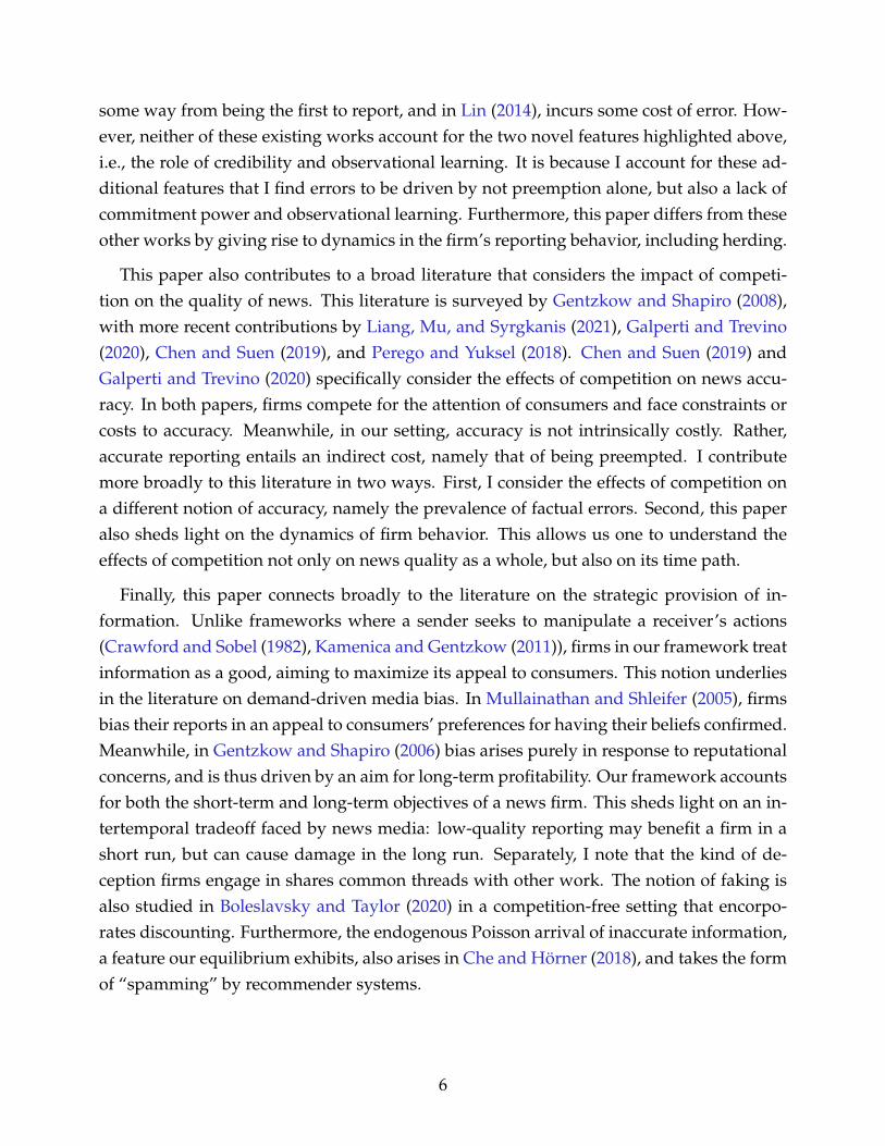
rise of digital news. Since the ascent of the internet, there has been a documented shiftfrom print to digital news.1 This shift is arguably contributing to a news industry wherefirms feel greater pressure to get stories out quickly in an effort to beat out competitors.This is due to the fact that, while print news is limited to daily publication at most, digitalnews faces no such constraints.2 By considering a continuous-time setting, one can betterunderstand 24-hour news environment, where preemptive concerns are not only presentbut ceaseless.

Analysis I analyze this model, establishing both existence and uniqueness of an equilib-rium. Under this equilibrium, fake reports do not occur at set times, but are rather dis-tributed continuously over time. This mixing implies an indifference condition: at any timein which faking might happen, the firm is indifferent between faking immediately and af-ter some short wait. Formally, this indifference condition implies an ordinary differentialequation (ODE) on the firm’s reporting behavior. I thus show that the equilibrium is char-acterized by a system of ODEs, a result which is central to our analysis and guides manyof the economic implications that follow.

Economic Implications I find that errors are strategic responses to two features of thenews environment: a lack of commitment by firms, and competition.

To this end, I begin by showing that competition alone is not responsible for reportingerrors. In particular, if the ex-post cost of errors is relatively small —because consumersare less aware or critical of them —even a monopolist will fake. Such errors are driven bya firm’s inability to commit to a reporting strategy: a firm is tempted fake after its credibilityhas been assessed. This is due to a moral hazard problem: consumers cannot observewhether a firm is faking, and thus there is no direct punishment for doing so. I substaniatethe notion that a lack of commitment causes errors by proving that a firm who can commitwill always report truthfully, and thus never err.

I then show that competition exacerbates errors, and does so through two separate chan-nels. First, competition can give rise to a preemptive motive in equilibrium. Namely, firmshave an incentive to speed up their reporting in order to beat out competitors. This incen-tive for speed induces firms to fake, and is thus responsible for reporting errors. Second,competition causes errors through another, less obvious channel: observational learning.When one firm reports a story, other firms become more confident that the story is true.

1 While 16% of 2018 survey respondents often receive news from print newspapers, 33% do so from newswebsites.

2 This is also true of TV news, which is the most popular news medium in the United States.

3

This increased confidence in turn yields firms more likely to fake and therefore err. I thusfind that observational learning exacerbates errors not by giving rise to them in the firstplace, but by causing an existing error to propagate through the market.

This paper also sheds light on the dynamics of reporting behavior and credibility. Thesedynamics take two different forms in equilibrium: gradual changes that happen in theabsence of new reports and sudden changes that occur in response to a new report.

I first show that firms become gradually more truthful —i.e., less inclined to fake—astime passes. Furthermore, firms become more credible over time whenever preemptive con-cerns are present. In other words, consumers are less trusting of reports that are madequickly. This model thus justifies consumers’ expressed concerns about hasty reporting.The reason for this gradual improvement in credibility lies in the firms incentives. The riskof being preempted introduces an endogenous cost to delay. Thus, the firm must some-how be compensated for this cost to ensure that its indifference condition is satisfied. Thisis achieved by means of increasing credibility. That is, increasing credibility mitigates thehaste-inducing effects of preemption.

In addition to this gradual increase in credibility, I find that dynamics can take a secondform: discrete changes in a firm’s reporting behavior and credibility in response to a rivalreport. This can entail a copycat effect, in which one firm’s report causes an instantaneousboost in faking by others. The copycat effect implies that when one firm’s report is quicklyrepeated by other firms, such follow-up reports will often lack credibility because they arenot independently verified. It illustrates that firms can herd on the reports themselves andthe timing of these reports. This provides an explanation for the “clustering” of reportingerrors that can occur in breaking news.3

In addition to these core results, I consider comparative statics and an extension of themodel. I find that, unsurprisingly, firms are more credible when there is a higher ex-postcost of error, and also when firms have a greater ability to learn. I also further explore therole of competition by considering the marginal effect of an additional firm in the market.I find that whenever preemptive concerns are present, adding a competitor will make eachindividual firm more likely to fake early on by increasing the preemptive threat they face.However, this is mitigated later on by the effects of observational learning: existing firmsare able to learn that the story is false more quickly by observing the silence of an additionalcompetitor, which will yield them less willing to fake. Finally, I extend the model to allowfor heterogeneity in firms’ ability to learn. This extended model gives rise to an intuitive

3 Examples of this include the reporting surrounding the Boston bombings and the 2000 US presidentialelection.

4

result: firms with greater ability to learn are also more credible in equilibrium. Thoughthere are many potential reasons why ability and accuracy can correlate in the market fornews, this model provides a novel reason for this: firms with lower ability face a greaterpreemptive threat, and are thus more willing to fake.

Related Literature. The preemption literature has modeled a variety of scenarios, includ-ing R&D races (Fudenberg, Gilbert, Stiglitz, and Tirole (1983)), technology adoption (Fu-denberg and Tirole (1985)), strategic exercise of options (Grenadier (1996)), and financialbubbles (Abreu and Brunnermeier (2003)). This paper contributes to this literature in twokey ways. The first is in the endogeneity of the payoff function. In the existing literature,a player’s decision to preempt does not affect its underlying payoff function. That is, thebenefit of preempting may be stochastic (e.g., Grenadier (1996)), but it is exogenous. In oursetting, however, a firm’s payoff from reporting hinges on the consumer’s beliefs aboutits reporting behavior. Such beliefs are important in the market for news because con-sumers may not be able to immediately observe the quality of a news report, e.g., whetherit was verified before bieng reported. This assumption has implications for the nature ofthe firm’s incentives. While in the existing literature, players earn some exogenous bene-fit from delaying their actions which counteracts the incentive to preempt, this is not truein our setting. Rather, I find that even if no such benefit exists exogenously, it will ariseendogenously.

This paper is not the first to consider observational learning in a preemption setting. InHopenhayn and Squintani (2011), firms can only observe their own payoffs, and thus drawinferences about the payoffs of their competitors by observing when and whether theyact. Meanwhile, in Bobtcheff, Bolte, and Mariotti (2017), players receive breakthroughswhich are privately observed, and thus at every moment are uncertain about how muchcompetition they face. In contrast, I assume that firms learn observationally about theirown payoffs, namely whether publishing the story will result in error. It is for this reasonthat observational learning gives rise to herding in this setting. It causes firms to herd onnot only on the decisions of their opponents but also in the timing of these decisions. Inthis sense, this paper also connects to the literature on herding with endogenously-timeddecisions (Gul and Lundholm (1995), Chamley and Gale (1994), Levin and Peck (2008)). Inparticular, notion that an action by one individuals can trigger others to quickly follow suitarises in Gul and Lundholm (1995). While such behavior is efficient in their setting, that isnot the case in ours, where it can cause errors to propagate through the market.

To my knowledge, there are two other papers which also consider preemption in break-ing news: Lin (2014) and Pant and Trombetta (2019). In both settings, a firm benefits in

5

some way from being the first to report, and in Lin (2014), incurs some cost of error. How-ever, neither of these existing works account for the two novel features highlighted above,i.e., the role of credibility and observational learning. It is because I account for these ad-ditional features that I find errors to be driven by not preemption alone, but also a lack ofcommitment power and observational learning. Furthermore, this paper differs from theseother works by giving rise to dynamics in the firm’s reporting behavior, including herding.

This paper also contributes to a broad literature that considers the impact of competi-tion on the quality of news. This literature is surveyed by Gentzkow and Shapiro (2008),with more recent contributions by Liang, Mu, and Syrgkanis (2021), Galperti and Trevino(2020), Chen and Suen (2019), and Perego and Yuksel (2018). Chen and Suen (2019) andGalperti and Trevino (2020) specifically consider the effects of competition on news accu-racy. In both papers, firms compete for the attention of consumers and face constraints orcosts to accuracy. Meanwhile, in our setting, accuracy is not intrinsically costly. Rather,accurate reporting entails an indirect cost, namely that of being preempted. I contributemore broadly to this literature in two ways. First, I consider the effects of competition ona different notion of accuracy, namely the prevalence of factual errors. Second, this paperalso sheds light on the dynamics of firm behavior. This allows us one to understand theeffects of competition not only on news quality as a whole, but also on its time path.

Finally, this paper connects broadly to the literature on the strategic provision of in-formation. Unlike frameworks where a sender seeks to manipulate a receiver’s actions(Crawford and Sobel (1982), Kamenica and Gentzkow (2011)), firms in our framework treatinformation as a good, aiming to maximize its appeal to consumers. This notion underliesin the literature on demand-driven media bias. In Mullainathan and Shleifer (2005), firmsbias their reports in an appeal to consumers’ preferences for having their beliefs confirmed.Meanwhile, in Gentzkow and Shapiro (2006) bias arises purely in response to reputationalconcerns, and is thus driven by an aim for long-term profitability. Our framework accountsfor both the short-term and long-term objectives of a news firm. This sheds light on an in-tertemporal tradeoff faced by news media: low-quality reporting may benefit a firm in ashort run, but can cause damage in the long run. Separately, I note that the kind of de-ception firms engage in shares common threads with other work. The notion of faking isalso studied in Boleslavsky and Taylor (2020) in a competition-free setting that encorpo-rates discounting. Furthermore, the endogenous Poisson arrival of inaccurate information,a feature our equilibrium exhibits, also arises in Che and Horner (2018), and takes the formof “spamming” by recommender systems.

6

Outline The remainder of the paper is organized as follows. Section 2 presents the model.Section 3 is dedicated to characterizing its equilibrium, first considering the monopolybenchmark and then the more general case where competition is present. In Section 4, Ipresent the core economic implications of this equilibrium, regarding both the effects ofcompetition and equilibrium dynamics. In Section 5, I present comparative statics. Section6 considers an extension of the model in which firms differ in their abilities to learn. Finally,Section 7 concludes. All formal proofs are relegated to the Appendix.

2. A model of breaking news

There are N ≥ 1 firms, indexed by i, and one consumer. Time, which is continuous andhas an infinite horizon, is denote by t ∈ [0,∞) . There is a time-invariant state θ ∈ {0, 1},which denotes whether a particular story is true (θ = 1) or false (θ = 0). All players areendowed with a common prior p0 ≡ Pr(θ = 1) ∈ (0, 1).

Each firm privately learns about the state by means of a one-sided Poisson signal: if θ =

1, a signal confirming this arrives to each firm at a Poisson rate λ > 0. This learning processcan be interpreted as one in which firms research the story by seeking confirmation that it istrue. I assume such a learning process because it serves as a reasonable approximation forthe learning that takes in a breaking news setting. For instance, a firm researching whetheran individual is the perpetrator of a terrorist attack can confirm this by discovering thatthey are either in custody or the subject of a search effort, but would find it much moredifficult to prove their innocence while the investigation is still ongoing. To formalize thislearning process, let si ∈ [0,∞] denote the time at which such a conclusive signal arrivesto firm i, with si =∞ denoting that a signal never arrives. I assume that si ∼ (1− e−λsi) ifθ = 1, and si = ∞ if θ = 0. We further assume that conditional on θ = 1, si is i.i.d. acrossfirms.

Each firm has a single opportunity to make a report over the course of the game. No-tably, the firm does not choose what to report, but instead whether and when to do so. Asthe payoff function will soon illustrate, the content of this report can be interpreted as anassertion that the story is true, i.e., that θ = 1. A report history H is a set {(i, ti)}i∈{1,...,N},pairing each firm i to the time at which it reported, ti, with ti = ∅ if the firm has not yetreported. Report histories are public information: at every time t, all players observe thecurrent report history. Thus, firms not only learn about θ via their private signal, but alsoobservationally by means of their rival firms’ reports.

A firm who never reports over the course of the game earns a payoff of 0. Meanwhile, a

7

firm who does report earnsknα− βI(θ = 0)

Let us now discuss the components of this payoff function. The first term, knα, capturesthe firm’s immediate payoff from making a report. This component captures the view-ership or readership the firm enjoys from reporting a story. This immediate payoff is aproduct of two separate components: kn and α. While kn captures the role of the firm’sorder n in its payoff, α denotes the credibility of the firm’s report.

Let us now formally define kn and α. A firm order of n denotes that the firm was thenth firm to report. We assume that the kn are constants, where k1 ≥ k2 ≥ ... ≥ kN ≥ 0. Thisassumption accounting for a key feature of the breaking news setting: competition. All elseequal, firms who report early compared to their competitors enjoy greater market share.The firm’s payoff is also increasing in the credibility of its report, α. A report’s credibility isthe consumer’s belief, at the time the report was sent, that the firm has received evidencethat θ = 1. Formally, this is the belief that si ∈ [0, t], where t is the time of the firm’s report.While the kn are exogenous parameters, α is an endogenous belief. In assuming this functionalform, we take the stance that a firm’s report will benefit it insofar that consumers believe itwas informed. This captures the notion that consumers value accuracy in journalism, andthus only consume news to the extent that they find it credible.

The second term, −βI(θ = 0), captures the ex-post penalty of an erroneous report: afirm who reports when θ = 0 incurs a penalty, given by a constant β > 0. This penaltycaptures the reputational harm a firm suffers from making a report that is later uncoveredto be false.

2.1. Equilibrium

For each belief p ≡ Pr(θ = 1) and order n ∈ {1, ..., N} of the next firm to report, denotesFp,n is a distribution over future report times: at each (p, n), let t denote the span of timethe firm waits before reporting conditional on not receiving a conclusive signal. Then, t isdistributed according to Fp,n ∈ ∆[0,∞], where t =∞ denotes a lack of report altogether. AMarkov strategy F is a collection of the Fp,n. I restrict attention to symmetric equilibria, andthus will omit the firm’s index from the Fp,n in much of the analysis below.

I place a number of restrictions on F . First, I assume that for all (p, n), Fp,n must bepiecewise twice differentiable and right-differentiable everywhere on [0,∞). This restric-tion both grants analytical convenience and ensures that all equilibrium objects are well-defined.

8

Second I impose a selection criterion (SC): a firm immediately reports once it has learnedthe story is true. Formally, this criterion is stated as follows

Definition 1. F satisfies (SC) if

F1,n(t) = 1 for all t ≥ 0, n ∈ {1, ..., N}.

This condition imposes that firms do not abstain from reporting a story they know to betrue. Importantly, it allows one to rule out equilibria with periods of silence supported byoff-path beliefs that reports made during these gaps entail zero credibility. An implicationof this assumption is that fixing any starting belief p, all players who have not yet reportedwill share the same common belief about the state after t time has passed. We denote thiscommon belief by p(t).

Finally, note that that defining strategies in this way, i.e. with a separate distribution foreach (p, n), is convenient, it introduces redudancy. Thus, we impose a consistency condi-tion to ensure that the Fp,n are consistent with each other whenever on-path.4 Specifically,this condition stipulates that Fp,n and Fp(t),n are related via the following formula:

Fp(t),n(s) =Fp,n(s+ t)− Fp,n(t−)

1− Fp,n(t−)for all s ≥ 0 whenever Fp,n(t) < 1, (1)

where Fp,n(t−) ≡ limτ↑t Fp,n(τ). This formula is an immediate result of Bayes Rule.

Before proceeding, we define two intuitive terms to describe both a report and the re-porting behavior of a firm: faking and truth telling. A report is fake if it is made by a firmdespite lacking independent confirmation, i.e., a signal si = ∅. Meanwhile, a report thatis made in response to such a signal is truthful. We use these terms to not only describe afirm’s report, but also its behavior: a firm is faking if it is sending a fake reports, while itis truth telling if its reports are exclusively truthful. Given the above selection assumption,strategies only differ in the distributions they place over fake reports.

We seek a symmetric perfect Bayesian equilibrium of this game. This is defined as aMarkov strategy F paired with beliefs α and p at each history such that F satisfies sequen-tial rationality and both α and p are consistent with Bayes Rule.

The consistency of α with Bayes Rule implies that it must be given by the followingformula at all (p, n) on-path: 5

4 This condition is analogous to the closed-loop property specified in Fudenberg and Tirole (1985). Weadopt the term consistency condition from Laraki, Solan, and Vieille (2005), who define this condition for ageneral class of continuous-time games of timing.

5 Formally, the formula is derived by applying Bayes Rule to a discrete-time approximation of the beliefs

9

αn(p) =

λp

λp+bn(p)if Fp,n(0) = 0

0 if Fp,n(0) > 0(2)

where bn(p) ≡ F ′p,n(0+) denotes the right-derivative of Fp,n at 0. That is bn(p) denotes theinstantaneous hazard rate of fake reports by a firm. This can be interpreted as the intensitywith which a firm fakes at a particular (p, n).

This formula is intuitive. If Fp,n(0) > 0, there exists a point mass of reports at (p, n).However, because conclusive signals are continuously distributed over time, the probabil-ity with which a valid report is made at (p, n) is zero. Thus, the consumer and all compet-ing firms know with certainty that a report made at (p, n) was fake, and thus assigns to it acredibility of zero. Meanwhile if there does not exist a point mass of reports at (p, n), credi-bility is assessed by comparing the instantaneous arrival rate of truthful reports (λp) to thatof fake reports (bn(p)), assigning a higher credibility to reports made when the hazard rateof fake reports is comparatively low.

3. Equilibrium characterization

3.1. Properties of equilibrium

We begin by establishing two necessary conditions on the firm’s equilibrium strategythat will guide the characterization that follows. Namely, we show that there there areno jumps and no gaps in the distribution of fake reports whenever credibility is less-than-perfect. These two properties, albeit in different forms, arise in other games with continu-ous strategy spaces.6 In this setting, these properties hold even in the absence of competi-tion. As I will illustrate below, this is due to the fact that these properties are not driven bycompetition, but by the endogeneity of the firm’s payoff.

These two properties are stated formally as Lemma 1:

Lemma 1. In equilibrium, at any (p, n) on-path Fp,n is

(a) continuous at all t whenever p < 1

(b) strictly increasing at any t such that αn(p(t)) < 1.

Let us begin by considering part (a) of Lemma 1, i.e., the “no jumps” property. This statesthat fake reports are distributed continuously over time whenever a firm is not certain

that obtain under this game. This derivation is presented in Appendix A.6 In particular, similar properties have been established in war of attrition games (Hendricks, Weiss, and

Wilson (1988)) and all-pay auctions (Baye, Kovenock, and De Vries (1996)).

10

that the story is true. That is, there can never be a point mass in faking. Notably, thisproperty holds even when competition is absent (n = 1). I will now argue that such pointmasses cannot occur because they give rise to a profitable deviation. This is driven by theassociation between the firm’s strategy and its credibility in equilibrium (2): reports thatare made whenever there is a point mass in faking yield zero credibility. Meanwhile, fakingwhile also not being certain than the story is true yields a strictly positive expected penaltyβ(1 − p). This implies that a firm’s value from faking at such a time is strictly negative.Thus, firm can profitably deviate by truth telling at that time: truth telling precludes thefirm from making an error, and therefore ensures a weakly positive payoff.

Next, we turn to part (b) of Lemma 1, the “no gaps” property. This states that wheneverthe firm is less-than-fully credible, the hazard rate of fake reports must be strictly posi-tive. In other words, firms must mix between faking at all times in which αn(p(t)) < 1.This property results directly from the formula for α (2): whenever credibility is less-than-perfect, the firm must be faking with at some positive rate bn(p). While straightforward,this property of the firm’s strategy has important implications for the firm’s incentives inequilibrium. In particular, it implies that whenever a firm’s credibility is less-than-perfect,it must be indifferent between faking instantly, and waiting an infinitesimal increment oftime before faking. This indifference condition is crucial to characterizing the firm’s behav-ior in equilibrium.

3.2. The monopoly benchmark and role of commitment

Before proceeding with the full model characterization, we consider the special case inwhich there is a single firm, i.e. n = 1. This serves two purposes. First, it elucidates theforces at play when competition is absent. In particular, it shows that errors can occur evenwithout competition, and that these errors are driven by a lack of commitment power bythe firm. Second, it serves as a benchmark for understanding the marginal impact compe-tition on both incentives and behavior.

We now state the monopoly characterization in terms of the firm’s credibility. Note thatbecause there is a single firm, we will drop the n index from all functions and parameters.

Claim 1. Under a monopoly, for all p on-path

α(p) = min{β/k, 1}

Claim 1 establishes two core facts about monopoly equilibrium. First, credibility is con-stant over time. As I will illustrate below, this contant credibility implies that the firm’s

11

reporting behavior is often not static. Specifically, the firm becomes more truthful overtime. Second, the monopolist’s credibility is weakly increasing in β, and is less-than-perfectwhenever β is sufficiently small. That is, errors occur even in the absence of competition,as long as the ex-post penalty from erring is sufficiently small. The remainder of this sub-section is dedicated to understanding why these two properties hold under a monopoly,and what they imply about the firm’s reporting behavior.

Let us begin by understanding why the firm’s credibility must be constant in equilib-rium. Recall that a firm must mix between faking at all times in which its credibility isless-than-perfect (Lemma 1(b)). Thus, whenever αn(p) < 1, the firm must find it optimal toboth fake immediately and after some short wait dt.7 By the martingale property of firm’sbelief p about the state, both of these strategies will yield the same expected penalty fromerror β(1 − p). Then, in order to ensure that both strategies are optimal, the firm’s prizefrom reporting must be the same as well. This implies that credibility must be constant inequilibrium. What is implicit in this reasoning is that in our setting, waiting is not costlyto a monopolist. In part this is because waiting is not intrisically costly to the firm, i.e.,future payoffs are not discounted. This is also due to the fact that a monopolist does notface competitors, and thus does not incur the implicit cost to waiting that comes from beingpreempted. In fact, when we discuss the equilibrium dyanamics (Subsection 4.1) it will beshown that a cost of preemption precludes α from being constant to equilibrium.

The constant nature of the monopolist’s credibility implies that its reporting behaviorwill often not be static. Namely, the hazard rate of faking (b) strictly decreases over time andtends to zero whenever credibility is less-than-perfect. That is, even when a firm fakes,it will become gradually more truthful over time. This is illustrated by Figure 1, whichgraphs b over time. While the decreasing nature of b follows directly from (2), there isalso an intuition behind this. Without observing a report, the consumer becomes graduallymore skeptical that the story is true. This is an artifact of the firm’s one-sided Poissonlearning process: the absence of a report means that firm has not received a conclusivesignal, and thus the common belief p(t) that the story is true decays over time.8 Thus, shebelieves truthful reports to become increasingly less probable. To ensure that the firm’scredibility remains constant, the hazard rate of fake reports must then decline as well, andeventually vanish.

Let us now consider the second property mentioned above, i.e., that a monopolist will

7 Implicitly, this relies on the assumption that αn(p(t)) is continuous over time: this ensures that ifαn(p) < 1, then αn(p(dt)) < 1 for dt sufficiently small. While we do not discuss this here, I formally es-tablish continuity in Appendix D (see Lemma 4).

8 Formally, in the monopoly case, p(t) = pe−λt

pe−λt+(1−p).

12

Figure 1: Hazard rate of fake reports in monopoly casewhen β < kn.

err with positive probability as long as the penalty of error is sufficiently small. This prop-erty demonstrates that competition alone is not responsible for errors in equilibrium. I nowargue that such errors are driven by a firm’s inability to commit to a reporting strategy.

To illustrate this point, let us first understand why truth telling cannot be sustainedwhen k > β. A firm that truth tells in equilibrium enjoys full credibility when making areport. Thus, the firm’s payoff from reporting when the story is false (θ = 0) is positive: theimmediate payoff of the report, k, strictly exceeds the penalty β from error. Consequently,faking is a profitable deviation. When θ = 1, both faking and truth telling will ensure thefirm reports eventually, earning a payoff of k. However, faking is strictly better for thefirm when θ = 0: it ensures a strictly positive payoff whereas truth telling yields nothing.The profitability of this deviation is driven by a moral hazard problem: because consumerscannot discern by merely observing a report whether it is fake. They only holds a beliefsin this regard, i.e., they assess credibility. While this assessment is made rationally basedthe beliefs about the firm’s strategy, the firm can always deviate after credibility has beendetermined. This is because the firm is unable commit to a reporting strategy, i.e., to forbiditself from deviating after the credibility has been assessed. Faking is especially temptingto the firm after its credibility has been assessed because it will not damage the firm’simmediate payoff of reporting.

Let us now consider how a monopolist firm would behave if it did had the ability tocommit. That is, suppose that the the firm could announce its strategy at the start of the

13

game, and was unable to deviate from that once credibility had been assessed.9 Under com-mitment, faking is more costly for the firm: it would always damage the firm’s credibility,and thus its immediate payoff from reporting.

One can immediately see that under commitment, the firm would always choose truth-telling over its non-commitment strategy when β < k. By committing to truth-telling, thefirm guarantees that it will earn a payoff of k if θ = 1, and 0 if θ = 0. Meanwhile, underno-commitment equilibrium, the firm will earn strictly less (β) when θ = 1, because it’scredibility will be strictly lower (β/k). Meanwhile, it will also earn 0 when θ = 0: thoughthe firm may fake, its payoff from faking is exactly equal to the penalty of error, meaningthat the firm will break even. In fact, one can show that truth-telling is not only better thanthe equilibrium strategy, but that it is the unique commitment solution under a monopoly.That is, given the ability to commit, a monopolist would never commit errors. This result,and its proof, is presented formally in Appendix F. We can thus conclude that a lack ofcommitment is responsible for errors under a monopoly. This also illustrates an importantpoint about a firm’s incentives: while commitment makes faking more costly for a firm, itin fact leaves the firm better off in equilibrium. This observation points to a larger themethat will persist even under competition: firms fake not because it intrinsically benefitsthem, but because it is a side effect of their strategic considerations.

3.3. Full model characterization

Here, I establish existence and uniqueness of an equilibrium in the full model. To thisend, I show that any equilibrium is the solution to a certain boundary value problem.Specifically, whenever the firm is not truthful, its credibility must satisfy an ODE and ap-propriate boundary condition. Characterizing the equilibrium in this way not only allowsone to establish existence and uniqueness, but lays the foundation for the economic analy-sis that follows.

We begin by establishing the precise conditions under which a firm is truthful. Wepresent this result for two reasons. First, it serves as a first step towards a full charac-terization. Second, while we illustrate this point more generally in the section that follows,this result shows how competition can deteriorate credibility and exacerbate faking.

Proposition 1. In equilibrium, at any (p, n) on-path, αn(p) = 1 if and only if the following twoconditions hold:

1. kn ≤ β

9 While we discuss the commitment solution informally here, a formal treatment is presented in Ap-pendix F.

14

2. p ≤ p∗n ≡ min{ kn−βkn

N−n+1−β , 1}

This result provides two conditions, on the model parameters and the common beliefabout the state, that are both necessary and sufficient for the firm to truth tell. The first con-dition, that kn ≤ β, was both necessary and sufficient for truth-telling under a monopoly(Claim 1). However, Proposition 1 asserts that when firms face competition, this conditionalone is not enough to ensure truth telling. A second condition is required: the commonbelief about the state must be sufficently low, lying below some threshold p∗n. That is, firmsmust be sufficiently skeptical about the validity of the story.

The necessity of this second condition illustrates an important point: truth telling is harderto sustain under competition. To understand why, note that truth telling is possible only ifthe firm does not have an incentive to deviate by faking. In the monopoly case, this wastrue as long as the cost of an incorrect report β outweighed the benefit from reporting(k). However competition introduces an additional cost to truth telling: the risk of beingpreempted. If a firm engages in truth telling, there is a risk that its opponent learns thestory is true, and thus reports first. A firm can evade this risk by faking, which ensures thatit won’t be preempted.

In the above reasoning, we took for granted that being preempted is costly for the firmwhenever it is truth-telling Let us now explain why this is the case. It is most obviousin the winner takes all case: all firms, with the exception of the first to make a report, areguaranteed to earn a payoff of zero, i.e., kn = 0 for all n > 1. In this case, the costliness ofbeing preempted is an artifact of the model parameters: a firm who is preempted will earnnothing from reporting. Generally, however, the decreasing nature of the kn alone doesnot guarantee that being preempted is costly: improved credibility for succeeding firmscould endogenously counteract the decay in the kn and make being preempted costless.However, one can show that being preempted must be costly for the firm whenever it istruth telling. This is due to the fact that truthfulness guarantees that the firm enjoys fullcredibility, which leaves no room for improvement in credibility.

Now, let us consider the significance of the second condition, i.e., that the firm will onlybe truthful if it is sufficiently pessimistic about the story’s validity. While truth telling en-tails a risk of being preempted, faking entails a different kidn of risk: that of making anerror and incurring penalty β. Both of these risks depend on the belief p about the state.A higher belief p is associated with both a lower risk of error and a higher risk of beingpreempted. Both of these make faking relatively more appealing to the firm, and conse-quently, make truth-telling more difficult to sustain. While it is immediate that a greaterp implies a smaller risk of error, that it implies a greater risk of being preempted is less

15

obvious. To see why, note that if the story is true, a competitor may preempt either becauseit has learned the story is true or it is faking. However, if the story is false, preemption istriggered solely by faking, and thus the risk of being preempted is lower. Thus, a firm whoholds a greater p will perceive its risk of being preempted to be greater.

While Proposition 1 pins down the conditions under which the firm is fully credible inequilibrium, it remains to characterize the firm’s behavior when truth telling does not hold.To this end, we obtain a key result: whenever not truth-telling, the firm’s credibility mustsatisfy a particular ODE and limit condition.

Proposition 2. In equilibrium, for all (p, n) on-path, if kn ≥ β, or p > p∗n ≡kn−βkn/n−β , then the

following ODE must be satisfied:

α′n(p) = − 1

kn(1− p)αn(p)

N − nN − n+ 1

[knαn(p)− Vp,n+1 − β(1− αn(p))(1− p)] (ODE)

where p ≡ αn(p) + (1− αn(p))p.

In addition, limp→0+ αn(p) = β/kn must hold if kn > β, and limp→p∗n+ αn(p) = 1 if kn ≤ β.

The proof for Proposition 2 relies critically on our above observation that whenever afirm is less-than-fully credible, it must mix between faking immediately and faking aftersome short wait, and thus must be indifferent between the two. To state this formally, let δsdenote the pure strategy distribution that places full mass on faking after s time has passed.In particular, δ0 denotes immediate faking, while δdt denotes faking after some short waitdt > 0. The indifference condition can then be written as follows:

Vp,n(δ0) = Vp,n(δdt)

where Vp,n(·) denotes the firm’s value from playing a particular strategy at (p, n).

To see how this indifference condition implies (ODE), note that a Taylor approximationof the firm’s value from waiting, Vp,n(δdt), yields the following:

Vp,n(δdt)− Vp,n(δ0) = [dp

dt(knα

′n(p))− λp(N − n)

αn(p)(Vp,n − Vp,n+1)]dt+ o(dt2) (3)

(3) is intuitive. It tells us that waiting to fake, rather than faking immediately, has twoimplications for the firm’s payoff. The first is that the firm’s credibility αn(p), and thusthe payoff enjoyed from reporting, may potentially change. This change in credibility isapproximated by dp

dt(knα

′n(p))dt. In addition, by waiting, the firm risks being preempted.

Precisely, with probability λp(N−n)αn(p)

dt the firm is preempted, in which case her expected

16

payoff will decline by Vp,n − Vp,n+1. We interpret this decrease in value as the firm’s costfrom being preempted.

Let us now examine both the probability and cost of preemption more closely. As onemight expect, the probability of being preempted is increasing in the number of rival firms(N − n) and the expected rate at which these rivals receives confirmation of the story (λp).Importantly, it is also decreasing in the equilibrium credibility. This is due to the fact thatlower credibility firms are more likely to fake, and thus pose a greater preemptive threat.

As for the firm’s cost of being preempted, let us begin by considering the second com-ponent of this expression, given by Vp,n+1. This denotes the firm’s continuation value in theevent that it is preempted. Importantly, being preempted not only affects the firm’s orderbut also the the common belief about the state. While the common belief was p prior to therival firm’s report, it increases to p ≡ αn(p) + (1− αn(p))p following the report. This is dueto observational learning. To understand why the common belief becomes p, note that arival firm’s report could mean one of two things: either the report was triggered by the ar-rival of a conclusive signal, in which case the story is certainly true, or it was not, in whichcase the report provides no new information and the belief remains p. The common belieffollowing this report is a weighted sum of these two conditional beliefs. In particular, theweight given to the rival firm’s report being informed by a conclusive signal is precisely itscredibility at the time of the report, αn(p). This new common belief will in turn determinethe firm’s continuation value in the event that it is preempted.

The cost of being preempted measures the impact of being preempted on the firm’scontinuation value. I.e., it measures how much the firm’s continuation value when it ispreempted differs from that in which it is not. Importantly, both continuation values areassessed at the common belief after being preempted, p. In this sense, we can view the costof being preempted as the firm’s ex-post regret from being preempted.

Note that in order for the indifference condition to be satisfied, the linear term of (3)must equal zero. This equality yields (ODE). That is, αn(p(t)) must change in preciselysuch a way that preserves the firm’s indifference condition.

In addition to establishing (ODE), Proposition 2 imposes a limit condition on the firm’scredibility. The precise limit condition that must hold depends on whether kn ≤ β, but al-ways applies at the boundary of the region in which the firm is faking. Let us first considerthe case where kn ≤ β. Recall from Proposition 1 that in this case, αn(p) = 1 wheneverp ≤ p∗n. We must then thus have that αn(p) limits to 1 as it approaches p∗n. If it did not,then as the belief approached p∗n, the firm could profitably deviate by not faking immedi-ately, and rather waiting until p∗n is reached to do so. Thus, this limit condition is needed

17

to sustain the firm’s indifference condition.

Let us next consider the case where kn > β. In this case, the firm never truth tells inequilibrium, and thus the indifference condition must always be satisifed. As the commonbelief p approaches zero, a firm who fakes does so being increasingly certain that its reportis erroneous, and thus expects to incur the full penalty β. Thus, the firm’s payoff fromfaking limits to the following:

limp→0+

Vp,n(δ0) = kn limp→0+

αn(p)− β

Separately, even though the firm sometimes fakes, it must also never fake, i.e., play strategyδ∞, with positive probability. This guarantees that the hazard rate of fake reporting remainslow enough to ensure that credibility remains sufficiently high, and thus that the firm willindeed find it optimal to fake.10 As p → 0+, the value of truth-telling tends to zero, asit becomes increasingly likely that the firm never reports. We can thus see that the limitcondition in this case, limp→0+ αn(p) = β/kn, is precisely what is need to ensure that thefirm is indifferent between faking and truth telling.

To take stock, Proposition 1 and Proposition 2 provide two different necessary condi-tions on equilibrium credibility. They establish a region under which truth telling mustoccur in equilibrium (Proposition 1), and show that otherwise, credibility must satisfy a re-cursive boundary value problem (Proposition 2). While we relegate this statement formallyto the appendix, one can show these two conditions are not only necessary, but sufficient,for an equilibrium.11 Establishing sufficiently entails showing that the firm cannot prof-itably deviate as long as its credibility satisfies these conditions. There is a clear intuitionfor this. On the region where truthfulness is necessary, it must also be optimal. This isfor the same reason that faking cannot occur on this region: the expected cost of erring isso high that it counteracts any benefit that faking might bring. Meanwhile on the regionwhere αn(p) < 1, the firm’s strategy involves faking. Faking is optimal on this region be-cause (ODE) guarantees it. In particular, it ensures firm’s indifference condition holds, i.e.,that faking at any such time is optimal.

We thus establish that the equilibrium is fully characterized by the solution to a recursiveboundary value problem. While we do not have a closed-form solution to this problem onthe region where αn(p) < 1, we are able to establish both existence and uniqueness of asolution. This is done by means of the Picard Theorem. This result is stated formally asTheorem 1.

10 We formalize this result in the Appendix as Lemma 2.11 This result is stated formally in the Appendix as Lemma 5.

18

Theorem 1. There exists a unique equilibrium (where uniqueness applies at (p, n) on-path).

4. Economic Implications

In this section, I consider the economic implications of this equilibrium. In particular, Iexplore two notions: (1) the dynamics of firm behavior and (2) the impact of competitionon both credibility and the prevalence of errors.

4.1. Equilibrium dynamics

In this section, I consider how a firm’s credibility and reporting behavior evolves overthe course of time. These results will not only illustrate when firms are most prone toerring, but will also allow us to better understand the endogenous nature of the firm’sincentives.

Dynamics take two separate forms in equilibrium: continuous changes as well as discretechanges. As we will show, continuous changes occur in the absence of any new reports,while discrete changes are triggered by a new report. More formally, let us denote a sub-game by a pair (p, n), where p denotes a starting belief and n the order of the next firmto report. We claim that fixing a subgame, i.e., assuming that no new firms report, thefirm’s credibility will change continuously over time. In particular it will gradually improvewhenever preemptive concerns are present. This result is stated formally as Proposition 3.

Proposition 3. For all (p, n) on-path, αn(p(t)) is weakly increasing in t. Furthermore,

1. If β > kN , then α′n(p(t)) > 0 whenever αn(p(t)) < 1.

2. If β ≤ kN , then αn(p(t)) is constant in t.

While αn(p(t)) must be constant under a monopoly, competition can introduce dynam-ics. In particular, Proposition 3 asserts that as long as αn(p(t)) has not reached its upperbound of 1, it is strictly increasing precisely when being preempted is costly to the firm.

Formally, this follows directly from (ODE). This is especially clear when we write (ODE)in the following form:

d

dtαn(p(t)) =

λp(N − n)

αn(p(t))kn[Vp,n − Vp,n+1]

We can see that αn(p(t)) must strictly increase over time whenever the cost of preemption,is strictly positive.

19

There is also a clear intuition for this result. Whenever the firm is less-than-fully cred-ible, it must be indifferent between faking immediately and waiting some period of timebefore doing so. However, if credibility remained constant, this indifference would failwhenever preemption is costly: the firm would obtain the same expected payoff from re-porting in both cases, but by reporting immediately would avert being preempted. Toensure that indifference is preserved, the firm must somehow be compensated for waiting.This must be achieved by means of strictly increasing credibility. While waiting presentsa cost to being preempted, a strictly increasing αn(p(t)) ensures that the firm’s report willbe rewarded more in the event that it is not preempted. Thus, the increasing nature ofαn(p(t)) is crucial to balancing the firm’s equilibrium incentives: it endogenously mitigatesthe haste-inducing effects of preemptive risk.

Let us now consider the implications of this result. It asserts that news reports thatare made with greater delay for research are generally more trustworthy in the eyes ofconsumers. That is, absent new reports by competitors, consumers will have greater trustin a firm’s journalistic standards when a report is not made quickly. In this sense, this resultconforms with consumers’ stated concerns about hasty reporting. This model provides ajustification for such concerns that are grounded in the firm’s incentives. Furthermore, bythe same reasoning presented in the monopoly section, the increasing nature of credibilitywithin a subgame implies that firms become gradually more truthful over the course of thegame. That is, bn(p(t)) is strictly decreases over time whenever the firm is not fully credible.

Finally, I note that while Proposition 3 asserts that αn(p(t)) must be strictly increasingwhen there is a cost to being preempted, this is not always the case. Specifically, whenkN ≥ β, being preempted is costless in equilibrium (i.e., Vp,n−Vp,n+1 = 0), and thus αn(p(t))

is constant. In other words, preemptive concerns endogenously disappear whenever theex-post cost of error, β, is sufficiently small. Formally, the credibility function will adjust insuch a way that ensures knαn(p) = kn+1αn+1(p) for all p. This highlights an notable featureof our model: competition alone does not imply preemptive concerns. Even if competitionis present, credibility can change in such a way that ensures preemption is costless.

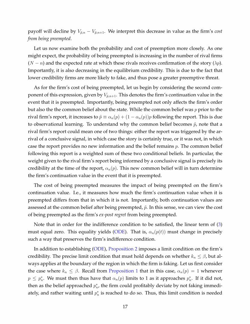
Let us now consider discrete changes in the firm’s credibility and faking. While credibil-ity changes continuously within a subgame, a rival report will cause the firm’s subgame tochange. That is, a report made at (p, n) will cause the order of the next reporter to increaseto n+1, and also cause the common belief to increase to p. This will in turn result in discretejumps in the firm’s credibility and faking rate (b). These discrete jumps are apparent in Fig-ure 2, which plots a simulation of α and b over the course of the game. As these graphsillustrate, jumps in both α and b are not monotonic. An opponent report may trigger eithera boost or decline in α and b. This is illustrated in Figure 2, while the first four reports cause

20

0.5

0.55

0.6

0.65

0.7

0.75

0.8

0.85

0.9

0.95

0

0.1

0.2

0.3

0.4

0.5

0.6

0.7

Figure 2: Simulations of crediblity and the hazard rate of fake reports, respectively, over the courseof the game. Discrete jumps in both graphs signify that a firm has made a report.

credibility to decrease and faking to increase, the fifth report causes credibility to decreaseand faking to increase.

These first four reports illustrate a copycat effect, in which one firm’s report causes animmediate a surge in the rate at which others fake.

To do so, first note that the discrete change in credibility that happens when a firm makesthe nth report under common belief p is given by the following:

αn+1(p)− αn(p)

where again p > p denotes the common belief in the immediate aftermath of the report.This expression shows that a report by one firm affects credibility by imposing two differ-ent changes to the environment. First, it impacts the order of the next firm, i.e., by ensuringthat the next firm to report will be the n+1th firm to report, rather than the nth. Secondly, itcauses discrete upwards jump in the common belief: firms will learn observationally fromthe report of their opponent, and thus become more confident about the story being true.The following decomposition isolates the respective impacts of these two changes:

αn+1(p)− αn(p) = [αn+1(p)− αn+1(p)]︸ ︷︷ ︸change in belief

+ [αn+1(p)− αn(p)]︸ ︷︷ ︸change in order

The effects of a change in order alone, αn+1(p) − αn(p), can have an ambiguous impact on

21

firms’ credibility in equilibrium. In particular, it hinges on the way in which the maximalprize kn changes with a firm’s order.

However, there is no ambiguity with regards to the effects of observational learning: itwill always cause a deterioration in credibility. Formally, αn+1(p) − αn+1(p) will alwaysbe negative in equilibrium, and strictly so whenever premeptive concerns are present (i.e.,whenever kN < β). This negative correlation between credibility and the firm’s belief thatthe story is true is also apparent in Proposition 3: later reports are associated with lowercommon beliefs about the story being true, and also with higher credibility. There is alsoa clear intuition to this: the more pessimistic the firm is about the story being true, thehigher its expected penalty from faking will be. This in turn will yeild the firm less willingto fake, and thus more credible in equilibrium. This illustrates that the downwards jumpsin credibility are caused, at least in part, by observational learning.

4.2. Effects of Competition

In this section, we consider the impact of competition on both credibility and fakingin equilibrium. We assess the impact of competition by comparing the equilibrium undercompetition (n ≥ 2) to that under the monopoly benchmark.

In order to isolate the effects of competition, we assume that the total ability of the mar-ket to learn is constant across these two cases. In particular, we assume that if each firmhas ability λ under competition, then the firm has ability nλ under the monopoly bench-mark. In making this normalization, we ensure that our comparison accounts for only theimpact of competition per se and does not confound this with the effects of an increasedaggregate ability to learn that firm entry may entail. We do however consider the effectsof market entry in the comparative statics section below, in which we do not normalize thetotal ability to learn.

Our findings are shown in Figure 3, which depicts both credibility and hazard rate offaking for a firm within a subgame, i.e., fixing a p and an n. The top and bottom rowshow the case where β ∈ (kN , kn) and β > kn, respectively. In both cases, we see that thatcompetition causes a deterioration in credibility and an increase in faking. Futhermore, this holdstrue for each individual firm. The effect of competition in this case is driven the cost ofpreemption that it induces. Firms are more inclined to fake, and thus less credible becausethe cost of preemption makes truth telling more costly for the firm. When β ∈ (kN , kn), thefirm fakes even under a monopoly, but strictly moreso under competition. That being saidthe effects of competition dissipate over time, as the competition level of credibility limitsto the monopoly value as time passes. Meanwhile, in the case where β > kn, a monopolist

22

Figure 3: Credibility αn(p(t)) (left) and the hazard rate of faking bn(p(t)) (right) under competitionand a monopoly. Top row depicts case where kn > β, while bottom row depicts case where β ∈(kN , kn).

firm will never fake, faking does temporarily occur under competition. Again, the effects ofcompetition are greatest early on with firms faking gradually less as time passes.

5. Comparative Statics

In this section, I consider how the equilibrium changes with the parameters of themodel. This will in shed light on how various features of the news market can contributeto, or curb, erroneous reporting. These findings are stated as Proposition 4.

Proposition 4. In any equilibrium, for any n, αn(p(t)) is

(a) weakly increasing in β, and strictly so whenever αn(p(t)) < 1.

23

(b) weakly increasing in λ, and strictly so for t > 0 whenever αn(p(t)) < 1 and kN < β.

(c) weakly decreasing in N , and strictly so whenever αn(p(t)) < 1, when t ∈ [0, t] for somet > 0.

Part (a) states that no matter when a firm reports, it will be more credible under highβ. This result is intuitive: a higher ex-post cost of error means firms are less likely to fake,and thus more credible. This result is a consequence of the firm’s equilbrium incentives: ahigher β makes faking more costly. This will either induce the firm to resort to truth-tellinginstead, or require that it is compensated for this coster faking with greater credibility.

Now, let us consider the comparative static on λ. This result is also intuitive: it statesthat credibility is higher when firms have a greater ability to learn. Let us now understandwhat is driving this result. We first note that at any belief p the firm may hold, a changein λ will have no effect on αn(p) in equilibrium. This is due to the fact that λ does not enterthe boundary value problem which dictates the firm’s credibility, and thus changes in λ

have no effect αn(p). However, changes in λ will have an effect on the time path of thecommon belief p(t). Under a higher λ, firms learn about the state more quickly, and thusp(t), the belief that θ = 1 conditional on no reports, will decay faster. That is, firms will bemore pessimistic about the story being true under a higher λ at any time t > 0. This greaterpessimism about the story translates to a higher expected cost of erring, thus making fakingmore costly. As was true for the comparative static on β, this increased cost of faking mustbe counterbalanced by a higher credibility αN(p(t)) at every time t > 0. This comparativestatic is illustrated by Figure 4, which shows simulations of the firm’s credibility functionunder high and low values of λ.

Let us finally consider the comparative static on the total number of firms N . While itpertains to the level of competition, this exercise is notably distinct from our analysis inthe previous section. Therein, we studied the overall impact of competition on equlibriumoutcomes. This was done by comparing the case where competition is present (N > 1) tothe monopoly case (N = 1) while holding constant the total learning ability of the market,Nλ. With this comparative static, we are instead considering the marginal impact of anadditional firm entering the market. In particular, we do not hold fixed total learningability of the market, and assume that this additional firm adds to the total learning abilityof the market. In doing so, we capture the effect of proliferation in the news industry.

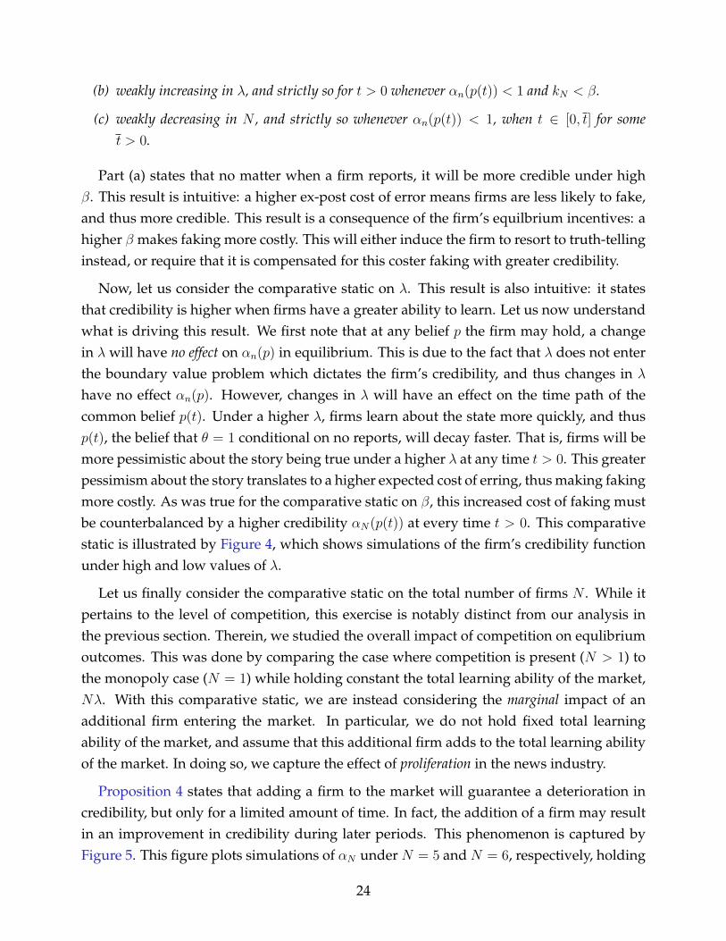
Proposition 4 states that adding a firm to the market will guarantee a deterioration incredibility, but only for a limited amount of time. In fact, the addition of a firm may resultin an improvement in credibility during later periods. This phenomenon is captured byFigure 5. This figure plots simulations of αN under N = 5 and N = 6, respectively, holding

24

Figure 4: A simulation of αN (p(t)) when λ = 1 (blue line)and λ = 0.5 (red line). For the remaining parameter values,the following specifications were made: β = 0.5, p0 = 0.7,N = 8, kn = 0.7(N−n).

all other parameters fixed. While the addition of a firm lowers credibility in early periods,it improves credibility in later periods.

To understand this result, we note that addition of a firm will effect two separate changesto the market. First, each firm faces greater competition, and thus a greater risk of beingpreempted. This change is precisely what was captured in our earlier exercise regardingthe effects of competition. As illustrated by Figure 3, this change will cause a deteriorationin credibility. However, an additional firm also increases the market’s total ability to learn.This change is captured by our comparative static on λ, which shows that an increase inthe market’s learning ability will cause an improvement in credibility. Thus the effect of anadditional firm can be understood as the combination of two countervailing forces: highercompetition and a higher ability to learn within the market.

To understand why the credibility-diminishing effect of higher competition must dom-inate in early periods, we must compare the relative magnitudes of these the two counter-vailing forces. Figure 4 illustrates that while credibility is pointwise higher at every t > 0

under high λ, this difference is negligible in early periods. This is due to the fact thatfirms learn gradually over time, and thus it takes time for differences in learning abilityto substantially impact firms’ beliefs. Meanwhile, as illustrated by Figure 3, an increasein competition will have a non-negligible impact on credibility even when t = 0. For thisreason, the impact of higher competition must dominate in early periods, resulting in a netreduction in credibility. However, as time passes and the effect of faster learning grows, a

25

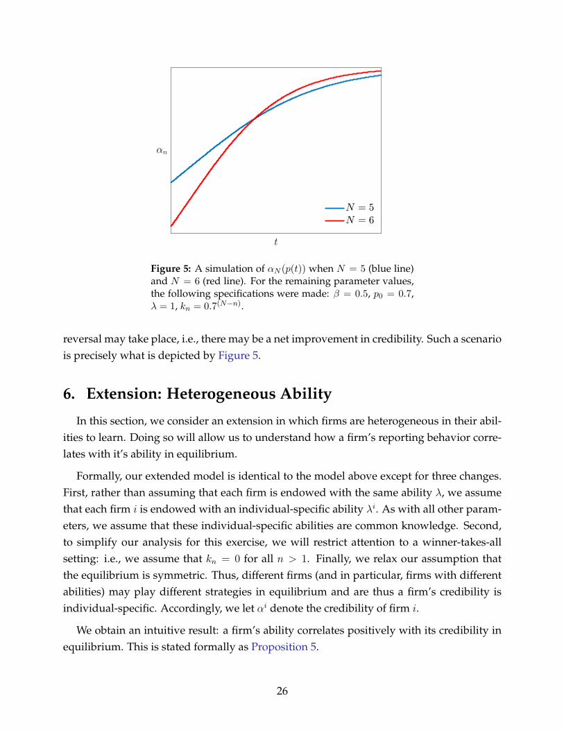
Figure 5: A simulation of αN (p(t)) when N = 5 (blue line)and N = 6 (red line). For the remaining parameter values,the following specifications were made: β = 0.5, p0 = 0.7,λ = 1, kn = 0.7(N−n).

reversal may take place, i.e., there may be a net improvement in credibility. Such a scenariois precisely what is depicted by Figure 5.

6. Extension: Heterogeneous Ability

In this section, we consider an extension in which firms are heterogeneous in their abil-ities to learn. Doing so will allow us to understand how a firm’s reporting behavior corre-lates with it’s ability in equilibrium.

Formally, our extended model is identical to the model above except for three changes.First, rather than assuming that each firm is endowed with the same ability λ, we assumethat each firm i is endowed with an individual-specific ability λi. As with all other param-eters, we assume that these individual-specific abilities are common knowledge. Second,to simplify our analysis for this exercise, we will restrict attention to a winner-takes-allsetting: i.e., we assume that kn = 0 for all n > 1. Finally, we relax our assumption thatthe equilibrium is symmetric. Thus, different firms (and in particular, firms with differentabilities) may play different strategies in equilibrium and are thus a firm’s credibility isindividual-specific. Accordingly, we let αi denote the credibility of firm i.

We obtain an intuitive result: a firm’s ability correlates positively with its credibility inequilibrium. This is stated formally as Proposition 5.

26

Proposition 5. For all (i, j) such that λi < λj , αi1(p(t)) ≤ αj1(p(t)). Furthermore, this inequalityis strict whenever αi1(p(t)) < 1.

Proposition 5 states that regardless of when a report is made, a firm with higher abilitywill be more credible.12 Furthermore, a high ability firm will be strictly more credible thana low ability firm whenever firms are not fully truthful.

Let us now understand why this correlation arises. First, note that high ability firms areable to confirm a story more quickly and thus, all else equal, pose a greater preemptivethreat in equilibrium. This in turn implies that in comparison to a high-ability firm, a low-ability firm faces a greater preemptive threat. This means that, all else equal, the low-abilityfirm finds immediate faking more advantageous. In light of this, the firms’ credibilitiesmust adjust in such a way to preserve their respective indifference conditions. This isachieved endogenously by means of a lower credibility for the low-ability firm, whichensures that it has less to gain from faking immediately.

7. Conclusion

In this paper, I presented a dynamic model of breaking news to understand the nature ofreporting errors. I sought to explain how strategic forces that could induce firms to err. Inthis setting, errors were driven by two qualities of the breaking news environment: a firm’slack of commitment power as well as competition. I find that competition induces firms toerr through two separate channels: preemptive motives and observational learning. Whilepreemptive motives can give rise to errors by encouraging firms to report hastily, observa-tional learning can cause an existing error to propagate through the market.

The second key objective was to understand the dynamics of reporting errors. In equi-librium, these dynamics take two forms. First, firms become gradually more truthful overtime as long as no new reports are made. Furthermore, a firm’s credibility gradually in-creases whenever preemptive motives are at play. Importantly, this improvement in cred-ibility incentivizes firms to take their time, and thus counteracts the haste-inducing effectsof preemption. Dynamics also take the form of discrete changes in the firm’s behavior andcredibility which are triggered by a rival report. In particular, I document a copycat effect,where a report by one firm can induce a surge in faking by other firms in the market.

While I consider breaking news specifically, this model provides broader insight intohow preemptive concerns can affect the quality of information provided by experts. To

12 This claim restricts attention to the first firm to report, because by the winner-takes-all assumption, allfollowing senders will never fake, i.e., αi

n(p) = 1 whenever n > 1.

27

understand how preemption impacts information provision more broadly is a topic thatwarrants further investigation.

References

Dilip Abreu and Markus K Brunnermeier. Bubbles and crashes. Econometrica, 71(1):173–204, 2003.

Michael R Baye, Dan Kovenock, and Casper G De Vries. The all-pay auction with completeinformation. Economic Theory, 8(2):291–305, 1996.

Catherine Bobtcheff, Jerome Bolte, and Thomas Mariotti. Researcher’s dilemma. The Re-view of Economic Studies, 84(3):969–1014, 2017.

Raphael Boleslavsky and Curtis R Taylor. Make it’til you fake it. Economic Research Initia-tives at Duke (ERID) Working Paper Forthcoming, 2020.

Pew Research Center. For local news, americans embrace digital but still want strong com-munity connection. Pew Research Center, 2019.

Christophe Chamley and Douglas Gale. Information revelation and strategic delay in amodel of investment. Econometrica: Journal of the Econometric Society, pages 1065–1085,1994.

Yeon-Koo Che and Johannes Horner. Recommender systems as mechanisms for sociallearning. The Quarterly Journal of Economics, 133(2):871–925, 2018.

Heng Chen and Wing Suen. Competition for attention and news quality. Technical report,working paper, 2019.

Vincent P Crawford and Joel Sobel. Strategic information transmission. Econometrica: Jour-nal of the Econometric Society, pages 1431–1451, 1982.

Drew Fudenberg and Jean Tirole. Preemption and rent equalization in the adoption of newtechnology. The Review of Economic Studies, 52(3):383–401, 1985.

Drew Fudenberg, Richard Gilbert, Joseph Stiglitz, and Jean Tirole. Preemption, leapfrog-ging and competition in patent races. European Economic Review, 22(1):3–31, 1983.

Simone Galperti and Isabel Trevino. Coordination motives and competition for attentionin information markets. Journal of Economic Theory, 188:105039, 2020.

28

Matthew Gentzkow and Jesse M Shapiro. Media bias and reputation. Journal of politicalEconomy, 114(2):280–316, 2006.

Matthew Gentzkow and Jesse M Shapiro. Competition and truth in the market for news.Journal of Economic perspectives, 22(2):133–154, 2008.

Jeffrey Gottfried, Mason Walker, and Amy Mitchell. Americans see skepticism of newsmedia as healthy, say public trust in the institution can improve. Pew Research Center,2020.

Steven R Grenadier. The strategic exercise of options: Development cascades and over-building in real estate markets. The Journal of Finance, 51(5):1653–1679, 1996.

Faruk Gul and Russell Lundholm. Endogenous timing and the clustering of agents’ deci-sions. Journal of political Economy, 103(5):1039–1066, 1995.

Ken Hendricks, Andrew Weiss, and Charles Wilson. The war of attrition in continuoustime with complete information. International Economic Review, pages 663–680, 1988.

Hugo A Hopenhayn and Francesco Squintani. Preemption games with private informa-tion. The Review of Economic Studies, 78(2):667–692, 2011.

Emir Kamenica and Matthew Gentzkow. Bayesian persuasion. American Economic Review,101(6):2590–2615, 2011.

Rida Laraki, Eilon Solan, and Nicolas Vieille. Continuous-time games of timing. Journal ofEconomic Theory, 120(2):206–238, 2005.

Dan Levin and James Peck. Investment dynamics with common and private values. Journalof economic Theory, 143(1):114–139, 2008.

Annie Liang, Xiaosheng Mu, and Vasilis Syrgkanis. Dynamically aggregating diverse in-formation. 2021.

Charles Lin. Speed versus accuracy in news. 2014.

Sendhil Mullainathan and Andrei Shleifer. The market for news. American economic review,95(4):1031–1053, 2005.

Ayush Pant and Federico Trombetta. The newsroom dilemma. Available at SSRN 3447908,2019.

Jacopo Perego and Sevgi Yuksel. Media competition and social disagreement. Work, 2018.

29

V Wang. Abc suspends reporter brian ross over erroneous report about trump. The NewYork Times, 2017.

Appendix A Discrete-time approximation of α

In this section, we formally justify equation (2), our equilibrium formula for αn(p), byshowing that it is the limit of Bayes-consistent beliefs under a discretized version of thegame presented in section (2). For any ε > 0, let the ε-approximation of the game beidentical to the game presented in section (2), except with the following modification: anyreport made by a firm on [0, ε] is observed by all other players (including the consumer) atε. Formally, rather than observing ti, the players observe ti, where

ti = max{ti, ε}

At any (p, n) that is on-path, let αεn(p) denote the firm’s credibility, i.e., the consumer’sbelief that si ≤ ε given that ti = ε, under the ε approximation of the game. Let us define αεnto be the right-limit of the αε, formally:

αn(p) ≡ limε→0+

αεn(p)

We now establish that on-path, αn(p) is given by (2).

Claim 2. For any (p, n) on-path,

αn(p) =

λp

λp+F ′p,n(0+)if Fp,n(0) = 0

0 if Fp,n(0) > 0

Proof. For any ε > 0, αεn(p, n) is uniquely determiend by Bayes Rule and given by

αε(p, n) =p(1− e−λε)

p(1− e−λε) + Fp,n(ε)e−λε.

First, consider the case where Fp,n(0) = 0. In this case, it follows from L’Hopital’s Rule that:

limε→0+

αε(p, n) =λp

λp+ F ′p,n(0+)

30

Next, consider the case where Fp,n(0) > 0. In this case, we obtain

limε→0+

αε(p, n) =0

0 + limε→0+ Fp,n(ε)= 0

where the final equality follows from the fact that limε→0+ Fp,n(ε) = Fp,n(0) > 0.

�

Appendix B Beliefs in equilibrium

We begin by stating some relevant properties and notation regarding the players’ beliefsabout the state.

First, we remark that at all times t and histories H , all players, with the exception ofthose who have already reported, must hold a common belief about the state. We omit aformal proof as this follows directly from our selection assumption that F1,n(0) = 1. Thisassumption implies that it is common knowledge that all firms who have not yet reportedhave not observed a conclusive signal. Thus, all such players, in addition to the consumer,share the same information set, and thus a common belief about the state.

Next, fixing an initial common belief p, and number of remaining firms n, we definetwo conditional beliefs, p(s) and pi(s), which we will reference frequently in the analysisthat follows. We let p(s) denote the common updated belief, conditional on no new reportsbeing made after s time passes. It follows from Bayes Rule that

p(s) =pe−nλs

pe−nλs + (1− p)(4)

Meanwhile, we let pi(s) denote the common updated belief, conditional on the eventthat player i report at s, and no other reports were made. Again, pi(s) follows directly fromBayes Rule, given α:

pi(s) = αn(p(s)) + (1− αn(p(s))p(s) (5)

To understand how pi(s) is computed, note that if a report is made after time s has passed,conditioning on the event that i’s report was informed, the common belief will update to1. However, conditioning on the event that i was uninformed when making the report,the report would have no impact on the common belief, which would thus be given byp(s). Thus, pi(s) is given by the weighted sum of these two beliefs, where the weighting isspecified by the belief that the report was informed, i.e., αn(p(s)).

31

Appendix C The firm’s problem

Before proceeding, we define a useful object, the first report distribution Ψ. Formally,fixing a (p, n), Ψi(s) denotes the probability that player i reported at or before s and was notpreceded by any of the remaining firms in doing so. Fixing a strategy profile (F 1

p,n, ..., Fnp,n),

it is given by:

Ψi(s) = p

∫ s

0

e−λr(N−n)∏j 6=i

(1−F jp,n(r))d(e−λr(F i

p,n(r)−1))+(1−p)∫ s

0

∏j 6=i

(1−F jp,n(r))dF i

p,n(r)

The first integral of the expression denotes the probability that i is the first firm conditionalon θ = 1, while the second integral denotes the same probability conditional on θ = 0.Ψi(s) is then the weighted sum of these two probabilities, where the weight is given by thecommon belief p about θ. Note that while Ψ is a function of the strategy profile, p, and n,we omit this dependence for brevity.

The firm’s problem is defined recursively as follows. Fix a firm i, n, p, α, and continua-tion value function V·,n+1. Trivially, Vp,0 = 0 for all p. Assume all firms j 6= i play the samestrategy F , and let−i to generically to refer to j 6= i. Then i’s expected payoff from playingstrategy F i at (p, n) is given by:

Vp,n(F i) =

∫ ∞0

[knαn(p(s))− β(1− pi(s))]dΨi(s) + (N − n)

∫ ∞0

Vp−i(s),n+1dΨ−i(s)

Note that first integral of this expression is firm i’s expected payoff from reporting, whenit is the first to do so. Meanwhile, the second integral is the firm’s expected payoff inthe circumstance where it is preempted. The firm’s problem at (p, n) is then given by thefollowing:

maxF i∈F

Vp,n(F i),

where F denotes the set of permissible distributions, i.e., those that are piecewise con-tinuously differenetiable, right-differentiable, and that satisfy the selection criterion. Wefurther define Vp,n = maxF i∈F Vp,n(F i).

Appendix D Regularity of F and α

Proof of Lemma 1. We will begin by showing that at all (p, n) on-path such that p < 1, Fp,nis continuous at 0. To this end, suppose by contradiction that Fp,n exhibits discontinuousat 0. By the right-continuity of Fp,n, Fp,n(0) > 0. Because (p, n) is on path, by (2), αn(p) = 0.Furthermore, it follows by (5) that pi(0) = p. Recalling that we are restricting attention

32

to symmetric equilibria, let Ψ denote the first-report distribution at (p, n) under the equi-librium strategy profile in which all firms who have not yet reported play Fp,n. BecauseFp,n(0) > 0, Ψj(0) > 0 for all j who have not yet reported.

Now define the following deviation Fp,n. This strategy is identical to Fp,n, except that allthe mass that Fp,n places on 0 is shifted to∞:

Fp,n(s) =

Fp,n(s)− Fp,n(0) if s <∞

1 if s =∞

Now, fix some iwho has not yet reported. Let Ψ denote the first-report distribution at (p, n)

under the strategy profile where i plays Fp,n and all j 6= i play Fp,n. By definition, for alls ≥ 0,

Ψi(s) = Ψi(s)−Ψi(0).

Thus∫ ∞0

[knαn(p(s))− β(1− pi(s))]dΨi(s) =

∫ ∞0

[knαn(p(s))− β(1− pi(s))]dΨi(s) + β(1− pi(0))Ψi(0)

>

∫ ∞0

[knαn(p(s))− β(1− pi(s))]dΨi(s).

Again by definition, for all s ≥ 0,

Ψ−i(s) = Ψ−i(s) +X(s),

where

X(s) ≡ Ψi(0)[p

∫ s

0

(1− Fp,n)n−2(1− Fp,n(r))e−λrd(e−λr(Fp,n(r)− 1))

+(1− p)∫ s

0

(1− Fp,n(r))n−2(1− Fp,n(r))dFp,n(r)]

Since X(s) is weakly increasing in s,∫ ∞0

Vp−i(s),n+1dΨ−i(s)−∫ ∞

0

Vp−i(s),N=1dΨ−i(s) =

∫ ∞0

Vp−i(s),n+1dX(s) ≥ 0.

where the final inequality follows from the fact that X(s) is increasing in s and Vp−i(s),n+1 ≥Vp−i(s),n+1(delta∞) ≥ 0.

33

Combining the above two inequalities we have

Vp,n(Fp,n) =

∫ ∞0

[knαn(p(s))− β(1− pi(s))]dΨi(s) + (N − n)

∫ ∞0

Vp−i(s),n+1dΨ−i(s)

>

∫ ∞0

[knαn(p(s))− β(1− pi(s))]dΨi(s) + (N − n)

∫ ∞0

Vp−i(s),n+1dΨ−i(s) = Vp,n(Fp,n)

Thus, i can profitably deviate at (p, n): contradiction.

We will now show that for all (p, n) on-path such that p < 1, Fp,n must be continuous atall t. Suppose by contradiction that it is not. Let t denote the time at which a discontinuityoccurs. Because Fp,n is increasing and right-differentiable by assumption, this must be ajump discontinuity, i.e.,

limr→t−

Fp,n(r) < Fp,n(t)

By (1),

Fp(t),n(0) =Fp,n(t)− limr↑t Fp,n(r)

1− limr↑t Fp,n(r)> 0.

But then, this implies that Fp(t),n is discontinuous at 0, contradicting the above.

Part (b) of the statement follows directly from (2). �

Lemma 2. For any (p, n) on-path,

• αn(p) ≥ αn(p) ≡ min{β(1− p)/kn, 1}

• F ′p,n(0+) ≤ f ≡ λp( 1α(p,n)

− 1)

Proof of Lemma 2. We begin by showing the first point above. The second point followsby definition of αn(p).

First, suppose by contradiction that there exists a (p, n) on-path such that

αn(p) < min{β(1− p)/kn, 1}

Recalling that p(s) is given by (4), we begin by claiming that for all s sufficiently small,(p(s), n) is on-path. Suppose not by contradiction. Since (p, n) is on-path by assumption,this implies that Fp,n(0) = 1, which contradicts Lemma 1. It thus follows from (2), combinedwith the piecewise twice differentiability and right-differentiability of Fp,n, that α(p(s), n)

is continuous in some right-neighborhood of s = 0. Formally, there exists an ε > 0 suchthat for all s ∈ [0, ε],

knαn(p(s)) < β(1− p).

34

Next, I claim that Fp,n(ε) > 0. Suppose this is not true by contradiction. Then, it followsthat Fp,n(s) = 0 for all s ∈ [0, ε], implying by definition of α that αn(p) = 1, contradictingour assumption that αn(p) < 1.

Now, define the following deviation Fp,n, which shifts the mass Fp,n places on [0, ε] to∞:

Fp,n(s) =

0 if s ∈ [0, ε]

Fp,n(s)− Fp,n(ε) if s ∈ (ε,∞)

1 if s =∞

The admissibility of Fp,n follows from the admissibility of Fp,n. We now wish to show thatFp,n is a profitable deviation at (p, n). Let Ψ denote the first-report distribution under thestrategy profile where all players play Fp,n, and let Ψ denote the first-report distributionunder the strategy profile where i plays Fp,n and all j 6= i play Fp,n.

By definition of Ψ,Ψi(s) = Ψi(s)−X(s)

where

X(s) =

p∫ s

0e−λr(N−n)(1− Fp,n(r))N−nd(e−λr(Fp,n(r)− 1)) + (1− p)

∫ s0

(1− Fp,n(r))N−ndFp,n(r) if s ∈ [0, ε]

X(ε) if s > ε

Now, note that X(s) is weakly increasing in s. Note further that because Fp,n(ε) ∈ (0, 1],it follows that Fp,n(s) strictly increases on [0, ε]. Thus, X(s) is strictly increasing at somes ∈ [0, ε]. Now, by the above definition:∫ ∞

0

[knαn(p(s))− β(1− pi(s))]dΨi(s)−∫ ∞

0

[knαn(p(s))− β(1− pi(s))]dΨi(s)

=

∫ ε

0

[knαn(p(s))− β(1− p(s))]dX(s) > 0

where the strict inequality follows from the fact that X(s) is strictly increasing on [0, ε] andthe above-established fact that knαn(p(s)) < β(1− p(s)) for all s ∈ [0, ε].

Next, let us examine Ψ(−i, s). It again follows from the definition of Ψ that

Ψ−i(s) = Ψ−i(s) = Y (s)

35

where

Y (s) = p

∫ s

0

[e−λr(1− Fp,n(r))]n−2F (min{r, ε})d(e−λr(Fp,n(r)− 1))+

(1− p)∫ s

0

(1− Fp,n(r))n−2Fp,n(min{r, ε})dFp,n(r)

Thus, ∫ ∞0

Vp−i(s),n+1dΨ−i(s)−∫ ∞

0

Vp−i(s),n+1dΨ−i(s) =

∫ ∞0

Vp−i(s),n+1dY (s) ≥ 0

where the final inequality follows for from the fact that Y (s) is increasing in s and Vp−i(s),n+1 ≥0. Combining the previous two inequalities, we obtain that

Vp,n(Fp,n) > Vp,n(Fp,n)

and thus i can profitably deviate at (p, n). Contradiction. �

Lemma 3. If αn(p) < 1 and (p, n) is on-path, then there exists an ε > 0 such that

Vp,n = Vp,n(δs) for all s ∈ [0, ε] ∪∞.

Proof of Lemma 3. Assume that αn(p) < 1. Note that by the right twice-differentiability ofFp,n, and by (2), that αn(p(s)) is right-continuous in s. Thus, there exists an ε > 0 and d > 0

such thatαn(p(s)) < 1− d for all s ∈ [0, ε].

I claim that for all s ∈ [0, ε), Vp,n = Vp,n(δs). Suppose to the contrary that for some s ∈ [0, ε),

Vp,n(δs) < Vp,n

Now, I claim that Vp,n(δs) is right-continuous in s. To see why this is the case, note that bydefinition,

Vp,n(δs) =

∫ s

0

knαn(p(r))dΨi(r) + (N − n)

∫ s

0

Vpi(r),ndΨ−i(r)+

(1−∑j

Ψj(s))[knα(p(s), n)− β(1− p(s))]

Where Ψj(s) is the first-report distribution that arises when i plays δ∞ and all j 6= i playFp,n. The right-continuity with respect to s then follows from the absolute continuity of Ψj

36

(which follows from Lemma 1), as well as the right-continuity of α(p(s), n) with respect tos, which follows from the right-continuity of Fp,n(s), which follows by assumption.

Given this right-continuity, some ε′ ∈ (0, ε− s) and x > 0 such that

Vp,n − Vp,n(δr) > x for all r ∈ [s, s+ ε′]

Note that there must exist some s∗ ∈ [0,∞] such that Vp,n = Vp,n(δs∗). Then, define thefollowing deviation Fp,n which shifts all the mass from [s, s + ε′] to s∗. Specifically, whens∗ < s:

Fp,n(t) =

Fp,n(t) + Fp,n(s+ ε)− Fp,n(s) if t ∈ [s∗, s]

Fp,n(s+ ε) if t ∈ (s, s+ ε′]

Fp,n(t) otherwise.

Meanwhile, when s∗ > s+ ε:

Fp,n(t) =

Fp,n(s) if t ∈ [s, s+ ε]

Fp,n(t)− [Fp,n(s+ ε′)− Fp,n(s)] if t ∈ (s+ ε′, s∗)

Fp,n(t) otherwise.

Now, by definition:

Vp,n(Fp,n) = Vp,n(Fp,n) +

∫ s+ε′

s

Vp,n(δs∗)− Vp,n(δr)dFp,n(r) ≥ Vp,n(Fp,n) + xε′ > Vp,n(Fp,n)

Thus, Fp,n serves as a profitable deviation. Contradiction.

It remains to show that Vp,n = Vp,n(δ∞). Suppose by contradiction that Vp,n > Vp,n(δ∞).It follows that limt→∞ Fp,n(t) = 0, because otherwise, the firm could profitably deviate byplacing no mass on t =∞. But this implies that for some s ∈ (0,∞],

limt→s−

F ′p,n(t+) =∞⇒ limt→s−

αn(p(t)) = 0,

which contradicts Lemma 2. �

Lemma 4. αn(p(s)) is continuous in s for all (p, n) on path such that s > 0.

Proof of Lemma 4. Fix a (p, n) on-path. I first claim that for all s ≥ 0,

αn(p(s)) =λp

λp+F ′p,n(s+)

1−Fp,n(s)

(6)

37

To see why this must hold, note that it follows from Lemma 2 that (p(s), n) is on-path forall s ≥ 0. Thus, by Lemma 1, Fp(s),n(0) = 0, and thus it follows from (2) that for all s ≥ 0,

αn(p(s)) =λp(s)

λp(s) + F ′p(s),n(0+).

Next, it follows from (1) that

F ′p(s),n(0+) =F ′p,n(s+)

1− Fp,n(s).

Combining the previous two equations yields (6). It thus follows from the right-continuityof Fp,n that αn(p(s)) is right-continuous in s. It remains to show that it is left-continuous.Suppose by contradiction there exists an s such that αn(p(s)) is left-discontinuous. Thenthere exists some d > 0 such that for all ε > 0, there exists an sε ∈ (s− ε, s) such that

|αn(p(sε))− αn(p(s))| > d.

First consider the case where for all ε > 0, αn(p(sε))−αn(p(s)) > d. I begin by claiming thatfor all ε > 0,

Vp(sε),n = Vp(sε),n(δs−sε). (7)

To this end, first note that there exists some s∗ ∈ (s,∞] such that Vp(sε),n = Vp(sε),n(δs∗,s∞). Tosee why this must hold, suppose not, by contradiction. Then it must be that Fp(sε),n placesfull support on [sε, s], and thus, either Lemma 1 or (2) would be violated. Thus, we have

Vp(sε),n =

∫ s−sε

0

knα(p(r))dΨi(r) + (N − n)

∫ s−sε

0

Vpi(r),n+1dΨ−i(r)+

(1−∑j

Ψj(s))Vp(s),n(δs∗−s) ≤∫ s−sε

0

knα(p(r))dΨi(r) + (N − n)

∫ s−sε

0

Vpi(r),n+1dΨ−i(r)

+(1−∑j

Ψj(s))Vp(s),n(δ0) = Vp(sε),n(δs−sε)

where Ψ is the first-report distribution associated witht he strategy profile in which i playsδ∞ and all j 6= i play Fp(sε),n. Note that the inequality follows from the fact that αn(p(s)) < 1,and thus by Lemma 3, Vp(s),n = Vp(s),n(δ0). However, note that for all ε > 0,

Vp(sε),n(δs−ε) =

∫ s−sε

0

knαn(p(r))dΨI(r) + (N − n)

∫ s−sε

0

Vpi(r),n+1dΨ−i(r)

+(1−∑j

Ψj(r))[knαn(p(s), n)− β(1− p(s))]

38

Because the Ψj are absolutely continuous,

limε→0

Vp(sε),n(δs−sε) = knαn(p(s), n)− β(1− p(s))

Thus, for all ε > 0 sufficiently small, Vp(sε),n(δ0) > Vp(sε),n(δs−sε), contradicting (7).

Next, consider the case where for all ε > 0, αn(p(s)) − αn(p(sε)) > d. As noted above,limε→0 Vp(sε),n(δs−sε) = Vp(s),n(δ0). Thus, for ε sufficiently small,

Vp(sε),n(δs−sε) > knαn(p(sε))− β(1− p(sε)) = Vp(sε),n(δ0)

However, since for all ε > 0, αn(p(sε)) < 1. By Lemma 3, Vp(sε),n = Vp(sε),n(δ0). Contradic-tion. �

Appendix E Characterization proofs

Proof of Proposition 1. We begin by showing that αn(p) = 1 whenever kn < β and p ≤p∗n ≡

kn−βkn/n−β .

To this end, fix any n, and suppose that kn < β. We begin by showing that for allq < β−kn

β, αn(q) = 1. Note that for all such q

Vq,n(δ0) = knαn(q)− β(1− q) ≤ kn − β(1− q) < kn − β(1− β − knβ

) = 0.

Since Vq,n ≥ Vq,n(δ∞) ≥ 0, it follows Vq,n > Vq,n(δ0). Thus, by Lemma 3, αn(q) = 1. Now, let

q∗n ≡ sup{p|αn(q) = 1 for all q < p}

It follows from the above that q∗n ≥β−knβ

> 0. Now suppose by contradiction that q∗n < p∗n.By Lemma 4, there exists an ε > 0 such that for all p ∈ (q∗n, q

∗n + ε), αn(p) < 1, and thus, by

Lemma 3Vp,n = Vp,n(δ0) = knαn(p)− β(1− p)

Thus, it follows from Lemma 4 that

limp→q∗n+

Vp,n = kn − β(1− q∗n) (8)

By definition of V , because by Lemma 1 Fp,n is absolutely continuous, it follows that

39

Vp,n(δ∞) is as well, and thus:

limp→q∗n+

Vp,n(δ∞) = Vq∗n,n(δ∞) =knq

∗n

n(9)

In for δ∞ to not serve as a profitable deviation for p ∈ (q∗n, q∗n+ε), it must be that for all such

p, Vp,n(δ0) ≥ Vp,n(δ∞). Taking a limit we obtain that

limp→q∗n+

Vp,n ≥ limp→q∗n+

Vp,n

Substituting (8) and (9) above, we obtain that knq∗nn≤ kn − β(1− q∗n). However, kn ≤ β and

q∗n < p implies that knq∗

n> kn − β(1− q). Contradiction.

Next, we show that αn(p) < 1 whenever β ≤ kn or p > p∗n. To this end, assume β ≤ kn

or p > p∗n. Assume by contradiction that αn(p) = 1. Also assume by induction that if n > 1,then the statement holds for n+ 1.

First, consider the case where αn(q) = 1 for all q < p. By (2), this implies that F ′(q, n) = 0.Furthermore, by Lemma 1, this implies that Fp,n(s) = 0 for all s > 0, i.e., Fp,n = δ∞.However,

Vp,n(δ0) = kn − β(1− p) > knp

n= Vp,n(δ∞),

where the above strict inequality follows from the above assumption that either β ≤ kn orp > p∗n.

Next, consider the case where αn(q) < 1 for some q < p. By Lemma 4, for all ε > 0

sufficiently small, there exists some p < p and s > 0 such that αn(p) ∈ (1 − ε, 1) and αn(q)

is strictly increasing on [p(s), p]. By Lemma 3, there exists some ∆ ∈ (0, s) such that

Vp,n(δ∆) = V (p, n, δ0).

By definition,

V (p, n, δ∆) =

∫ ∆

0

knαn(p(s))dΨi(s) + (N − n)

∫ ∆

0

V (pi(s), n+ 1)dΨ−i(s)+

(1−∑j

Ψj(∆))(knαn(p(∆))− β(1− p(∆))

where Ψ is the first-report distribution associated with the strategy profile where i plays δ∆

40

and all j = i play Fp,n. Meanwhile,

V (p, n, δ0) = knαn(p)− β(1− p)

=

∫ ∆

0

knαn(p)dΨi(s) + (N − n)

∫ ∆

0

knαn(p)− β(1− pi(s))dΨ−i(s)

+ (1−∑j

Ψj(∆))(knαn(p)− β(1− p(∆))

Thus, in order to preserve the above equality, for some r ∈ (0, s),

knαn(p)− β(1− pi(r)) < V (pi(r), n+ 1). (10)

First, consider the case where αn+1(pi(r))) < 1. Then, for ε > 0 sufficiently small

Vpi(r),n+1 = Vpi(r),n+1(δ0) = kn+1αn+1(pi(r))− β(1− pi(r)) < knαn(p)− β(1− pi(r))

where the first equality follows from Lemma 3. Thus, equation (10) is violated. Contradic-tion.

Next, consider the case where αn+1(pi(r)) = 1 and β < kn. By the inductive assumption,it follows that αn+1(q) = 1 for all q ≤ pi(s). Thus, Fpi(s),n+1 = δ∞. So, we have that for εsufficiently small:

Vpi(r),n+1 = Vpi(r),n+1(δ∞) =kn+1p

i(r)

N − n≤ pi(r)knαn(p) + (1− pi(s))knαn(p)− β)

= knαn(p)− β(1− pi(s))

Again, this is a contradiction of (10).

Finally, consider the case where αn+1(pi(r)) = 1 and β ≥ kn. Recall by Proposition 1 thatαn(q) = 1 for all q ≥ p∗n. Thus, because αn(p) < 1, it follows from (4) that αn(p(s)) must bestrictly increasing in s for some s > r. Formally, let

r′ = inf{s > r|αn(p(s)) is strictly increasing}.

First, we claim thatknαn(p(r′))− β(1− pi(r)) < Vpi(r),n+1 (11)

By the inductive assumption, since αn+1(pi) = 1, it must be that αn+1(q) = 1 for all q < pi(r).Because αn(p(s)) is weakly decreasing for s ∈ [r, r′], it follows by definition of pi(s) that

41

pi(s) < pi(r) for all s ∈ [r, r′]. Thus, for all s ∈ [r, r′]

Vpi(s),n+1 =kn+1p

i(s)

N − n.

It follows from this that for all s ≥ r,

knαn(p(s))− β(1− pi(s)) < Vpi(s),n+1

⇔ knαn(p(s))− β(1− pi(s)) < kn+1pi(s)

N − n

⇔ pi(s) <β − knαn(p(r))

β − kn+1/(N − n)

Now, because αn(p(s)) is strictly decreasing on s ∈ [0, r].

knαn(p(r))− β(1− pi(r)) < knαn(p)− β(1− pi(r)) < Vpi(r),n+1

where the second inequality was established above. Thus we have

pi(r′) < pi(r) <β − knαn+1(p(r))

β − kn+1/(N − n)<β − knαn+1(p(r′))

β − kn+1/(N − n)

which implies (11).

It follows from this that there exists an r′′ > r′ such that for all s ∈ [r′, r′′], αn(p(s)) isweakly decreasing and Vpi(s),n+1 > knαn(p(r′))− β(1− pi(s)). Now I claim that

Vp(r′),n(δ0) < Vp(r′),n(δr′′−r′).

To see why this must be true, note that by definition,

Vp(r′),n(δr′′−r′)− Vp(r′),n(δ0) =

∫ r′′

r′kn[αn(p(s))− αn(p(r′))]dΨ(i, s)+∫ r′′

r′[Vpi(s),n+1 − (knαn(p(r′))− β(1− pi(s)))]dΨ−i(s)

+∑j

(Ψ(j, r′′)−Ψ(j, r′))kn(αn(p(r′′))− knαn(p(r′)))

Since αn(p(s)) ≥ αn(p(r′)) and Vpi(s),n+1 > knαn(p(r′)) − β(1 − pi(s)) s ∈ [r′, r′′], it followsthat Vp(r′),n(δr′′−r′)− Vp(r′),n(δ0) > 0. However, this contradicts Lemma 3. �

Proof of Proposition 2. Proof by induction. Fix an n, and assume that αm(p) satisfies the

42

above for all m < n such that (p,m) is on-path.

We begin by showing that (ODE) must hold whenever αn(p) < 1. To this end, assumethat αn(p) < 1. Then, by Lemma 3, there exists an ε > 0 such that for all ∆ ∈ (0, ε),

Vp,n(δ∆)− Vp,n(δ0)

∆= 0 (12)

Recall that by definition of V , that

Vp,n(δ0) = knαn(p)− β(1− p).

Meanwhile

Vp,n(δ∆) =

∫ ∆

0

knαn(p(s))Ψ(i, s)ds+ (N − n)

∫ ∆

0

Vp−i(s),n+1Ψ(−i, s)ds+

(1−∑j

lims→∆−

Ψ(s, j))[knαn(p(∆))− β(1− p(∆))]

where Ψ is the first-report distribution associated with the strategy profile in which i playsδ∞ and all j 6= i play F j

p,S . Specifically, for all s > 0,

Ψi(s) = pλ

∫ s

0

e−λrn(1− Fp,n(r))N−ndr

Ψ−i(s) = p

∫ s

0

e−λr(N−n)(1−Fp,n(r))n−2d(−e−λr(1−Fp,S(r)))+(1−p)∫ s

0

(1−Fp,n(r))n−2dFp,n(r)

Note that it follows from Lemma 1 that, for all j, Ψj is also absolutely continuous, I.e., thereexists a function ψj such that:

Ψj(s) =

∫ s

0

ψj(r)dr.

Specifically, according to Lemma 1, one such ψi and ψ−i are given by the following:

ψi(s) = pλe−λsn(1− Fp,n(s))N−n

ψ−i(s) = pe−λsn(λ+ F ′p,n(s+)− λFp,n(s))(1− Fp,n(s))n−2 + (1− p)(1− Fp,n(s))F ′p,n(s+)

Substituting these expressions for both Vp,n(δ0) and Vp,n(δ∆) into (12) and rearranging, weobtain that for all ∆ ∈ (0, ε),

K1(∆) +K2(∆) +K3(∆) = 0 (13)

43

where

K1(∆) ≡∫ ∆

0kn[(αn(p(s))− αn(p)) + β(1− p)]ψi(s)ds

∆

K2(∆) ≡(N − n)

∫ ∆

0[Vp−i(s),n+1 − knαn(p) + β(1− p)]ψ−i(s)ds

∆

K3(∆) ≡(1−

∑j lims→∆− ψj(∆))[kn(αn(p(∆))− αn(p)) + β(p(∆)− p)]

∆

Now, we consider lim∆→0+ of K1(∆), K2(∆), and K3(∆) separately.

For K1(∆), it follows from L’Hopital’s Rule, together with the continuity of αn(p(∆))

(i.e., Lemma 4) and ψi(∆) in ∆ that

lim∆→0+

K1(∆) = lim∆→0+

[kn(αn(p(∆))− αn(p)) + β(1− p)]ψi(∆) = β(1− p)ψi(0) = β(1− p)pλ.

For K2(∆), it again follows from L’Hopital’s Rule, together with the right-continuity ofVp−i(∆),n+1 in ∆ that

lim∆→0+

K2(∆) = (N − n) lim∆→0+

[Vp−i(∆),n+1 − knαn(p) + β(1− p)]ψ−i(∆)

= (N − n)[Vp−i,n+1 − knαn(p) + β(1− p)]( λp

αn(p))

where the final inequality follows from the fact that at all (p, n) on-path, αn(p) = λpλp+F ′p,n(0)

.

For K2(∆), first note that by the continuous differentiability of Ψj(s) that

lim∆→0+

∑j

lims→∆−

Ψ(s, j) = 0.

Thus, it follows from the right-differentiability of αn(p(∆)) in ∆ that

lim∆→0+

K3(∆) = kn lim∆→0

αn(p(∆))− αn(p)

∆+ β lim

∆→0+

p(∆)− p∆

= knd

d∆αn(p(∆))

∣∣∣∆=0+

+ βp′(∆)∣∣∣∆=0+

= p′(∆)∣∣∣∆=0+

[knα′n(p) + β] = −λpn(1− p)[knα′n(p) + β]

Since we have shown that lim∆→0+ K1(∆), lim∆→0+K2(∆), and lim∆→0+K3(∆) exist, andare given by the above expressions, it follows from (13) that

lim∆→0+

K1(∆) + lim∆→0+

K2(∆) + lim∆→0+

K3(∆) = 0.

44

Substituting in the above expressions for K1(∆), K2(∆) and K3(∆), we obtain (ODE).

Now, we wish to establish that (ODE) must hold whenever kn ≥ β or p > p∗n. It followsfrom Proposition 1 that αn(p) < 1, and thus by the above, (ODE) must hold.

Finally, we establish the two limit conditions presented in the proposition. We begin byestablishing that when kn ≥ β, limp→0+ αn(p) = β/kn. To this end, first note by Lemma 3that for all p > 0, Vp,n(δ0) = Vp,n(δ∞). Note further that

limp→0+

Vp,n(δ∞) = 0.

Thus,limp→0+

Vp,n(δ0) = limp→0+

knαn(p)− β = 0,

and therefore, limp→0+ αn(p) = βkn

. Next, let us consider the case where kn < β. Thatlimp→p∗n+ αn(p) = 1 follows from Lemma 4, since by Proposition 1, αn(p∗n) = 1. �

Definition 2. α is a solution to (P) if it satisfies the following for all n ≤ N and p ∈ (0, 1]:

• If kn < β and p ≤ p∗n ≡kn−βkn/n−β , then αn(p) = 1.

• If kn ≥ β or p < p∗n, then α satisfies (ODE), with limit condition limp→0+ αn(p) = β/kn

if kn ≥ β and limp→pn∗+ αn(p) = 1 if kn < β.

• αn(1) = 0.

Lemma 5. (α, F ) is an equilibrium if and only if at all (p, n) on-path, α is both consistent with Fand a solution to (P).

Proof of Lemma 5. Fix an (α, F ). We begin by establishing the necessity of the three con-ditions specified in Definition 2 for (α, F ) to be an equilibrium. First we establish the ne-cessity of the first bullet of Definition 2. To this end, recall that by the selection assumption,F1,n(0) = 1. Thus, it follows from (2) that αn(1) = 0 if (p = 1, n) is on-path. Bullets two andthree of Definition (2) follow from Proposition 1 and Proposition 2, respectively.

Next, we establish the sufficiency of the above conditions for (α, F ) to be an equilibrium.We begin by considering the case in which kn < β and p ≤ p∗n. It follows from (P) thatαn(q) = 1 for all q ≤ p. Thus, by (2), Fp,n = δ∞. We thus wish to show that there exist noprofitable deviations in this case, i.e., that Vp,n = Vp,n(δ∞). It suffices to show that

Vp,n(δ∞) ≥ Vp,n(δs) for all s ∈ [0,∞). (14)

45

First, note that for all s ∈ (0,∞),

Vp,n(δs) = kn(1− p(1− e−λsn)(N − n

N − n+ 1))− β(1− p) ≤ kn − β(1− p) = Vp,n(δ0).

Further, kn ≤ β and p ≤ p∗n implies that

Vp,n(δ0) = kn − β(1− p) ≤ knn

= Vp,n(δ∞)

Thus, Vp,n(δ∞) ≥ Vp,n(δs) for all s ∈ [0,∞)

Next, we show that Fp,n is optimal when kn ≥ β or p < p∗n. To this end, we begin byshowing that

d

d∆Vp,n(δ∆) = 0 for all ∆ ∈ [0,∞) if kn ≥ β and for all ∆ ∈ [0, t∗) if kn < β (15)

where t∗ is the unique value such that p(t∗) = p∗n. Note that

Vp,n(δ∆) =

∫ ∆

0

knαn(p(s))dΨi(s) +

∫ ∆

0

Vpi(s),n+1dΨ−i(s)+

(1−∑j

Ψj(∆))(αn(p(∆))− β(1− p(∆)))(16)

where Ψ is the first-report distribution associated with the strategy profile in which i playsδ∞ and all j 6= i play Fp,n. Then, it follows that

d

d∆Vp,n(δ∆)

= knαn(p(∆))Ψi′(∆) + (N − n)Vpi(∆),n+1Ψ−i′(∆) + (1−∑j

Ψj(∆))p′(∆)[α′n(p(∆))− β]

−∑j

Ψj′(∆)(knαn(p(∆))− β(1− p(∆)))

= (N − n)[Vpi(∆),n+1 − knαn(p(∆)) + β(1− p(∆))]Ψ−i′(∆)− β(1− p(∆))Ψi′(∆)

+ (1−∑j

Ψj(∆))p′(∆)(knα′(p(∆), n)− β)

Note that in the above, the existence of Ψj′(∆) follows from the differentiability of αnat p(∆), and thus, the differentiability of Fp,n at ∆. We wish to show that d

d∆Vp,n(δ∆) = 0.

To this end, we begin by deriving expressions for Ψi′(∆) and Ψ−i′(∆). First, it follows by

46

definition of the first-report distribution that:

Ψi(∆) = pλ

∫ ∆

0

(1− Fp,n(s))N−ne−λnsds.

Differentiating this, we obtain:

Ψi′(∆) = pλ(1− Fp,n(∆))N−ne−λn∆

Meanwhile:

Ψ−i(∆) = p

∫ ∆

0

(1−Fp,n(s))n−2e−λ(N−n)sd((Fp,n(s)−1)e−λs)+(1−p)∫ ∆

0

(1−Fp,n(s))n−2F ′p,n(s)ds

where the existence of F ′p,n(s) again follows from the assumption that αn is differentiableat p(s). Differentiating this, we obtain:

Ψ−i′(∆) = p(1− Fp,n(∆))n−2e−λ∆n[F ′p,n(∆) + λ(1− Fp,n(∆))] + (1− p)(1− Fp,n(∆))n−2fp,n(∆)

= (1− Fp,n(∆))N−n[fp,n(∆)

1− Fp,n(∆)(pe−λ∆n + (1− p)) + pe−λ∆nλ]

It follows from the definition of α (equation (2)) and the consistency condition (equation(1)) that

F ′p,n(∆)

1− Fp,n(∆)= λp(∆)(

1

αn(p(∆))− 1).

Substituting this, along with the definition of p(∆) (equation (4)), we obtain:

Ψ−i′(∆) = λ(1− Fp,n(∆))N−n(pe−λ∆n + (1− p)) p(∆)

αn(p(∆))

Note further that

1−∑j

Ψj(∆) = (1− F (∆))N−n(pe−λ∆n + (1− p)) (17)

Substituting equations the expressions for Ψi′(∆), Ψ−i′(∆), and 1 −∑

j Ψj(∆) into theabove equation for d

d∆Vp,n(δ∆), and simplyifying, we obtain:

d

d∆Vp,n(δ∆) = K[

(N − n)

αn(p(∆))(V i(p(∆), n+ 1)− knαn(p(∆)) + β(1− p(∆))(1− αn(p(∆))))

−knα′(p(∆), n)(1− p(∆))n]

47

whereK ≡ λ(1−Fp,n(∆))N−n(pe−λ∆n+(1−p))p(∆). Because (ODE) is satisfied at (p(∆), n),using it to substitute in for α′(p(∆, n), we obtain (15).

Now, consider the case where kn ≥ β. To show Fp,n is optimal, it suffices to show thatall pure strategies δ∆ yield the same payoff, i.e., that

Vp,n(δ0) = Vp,n(δ∆) (18)

for all ∆ ∈ [0,∞]. It follows directly from (15) that (18) holds for all ∆ ∈ [0,∞). It remainsto show that (18) holds for ∆ =∞. To this end, first note that by (15),

Vp,n(δ0) = lim∆→∞

Vp,n(δ∆)

= lim∆→∞

∫ ∆

0

knαn(p(s))dΨi(s) + (N − n) lim∆→∞

∫ ∆

0

V (pi(s), n+ 1)dΨ−i(s)+

lim∆→∞

(1−∑j

Ψj(∆))(knαn(p(∆))− β(1− p(∆)))

=

∫ ∞0

knαn(p(∆))dΨi(s) + (N − n)

∫ ∞0

V (pi(∆), n+ 1)dΨ−i(s) = Vp,n(δ∞)

where the third equality follows from the limit condition limp→0+ α(p, n) = β/kn:

lim∆→∞

knαn(p(∆))− β(1− p(∆)) = limp→0+

knαn(0)− β = 0.

Finally, consider the case where kn < β and p > p∗n. Note that because αn(p(s)) = 1 for alls > t∗, by (2), it follows that F ′p,n(s) = 0 for all such s. It follows from this that the supportof Fp,n lies within [0, t∗] ∪ ∞. Thus, to show Fp,n is optimal, it suffices to show that δ∆ isoptimal for ∆ ∈ [0, t∗] ∪∞. To this end, we will proceed by first showing

Vp,n(δ∆) = Vp,n(0) for all ∆ ∈ [0, t∗] ∪∞ (19)

and then showingVp,n(δt∗) ≥ Vp,n(δ∆)for all ∆ ∈ (t∗,∞). (20)

To show (19), first recall that it follows from (15) that

Vp,n(δ0) = Vp,n(δ∆) for all ∆ ∈ [0, t∗).

It remains to show Vp,n(δ0) = Vp,n(δs) for s ∈ {t∗,∞}. For s = t∗, note that it follows from

48

the above thatVp,n(δ0) = lim

∆→t∗−Vp,n(δ∆) = Vp,n(δt∗)

where the final inequality follows from (16), observing that αn is continuous at p∗n and Ψj

is continuous at t∗. We will now show Vp,n(δt∗) = Vp,n(δ∞). To this end, note that for all∆ ∈ [t∗,∞]:

Vp,n(δ∆) =

∫ t∗

0

knαn(p(s))dΨi(s)+(N−n)

∫ t∗

0

V (pi(s), n+1)dΨ−i(s)+(1−∑j

Ψj(t∗))V (p∗n, n, δ∆−t∗)

Thus, to show V (p, n, δ∗t ) = Vp,n(δ∞), it suffices to show that V (p∗n, n, δ0) = V (p∗n, n, δ∞). Butit follows from the definition of p∗n that:

V (p∗n, n, δ0) = kn − β(1− p∗n) =knp

∗n

n= V (p∗n, n, δ∞).

Similarly, to show (20), it suffices to show that V (p∗n, n, δ0) ≥ V (p∗n, n, δ∆) for all ∆ ∈(0,∞), which we had previously established in (14). �

Proof of Theorem 1. Fix an n. Assume inductively that there exists a unique solution to (P)for all m < n. We wish to show that ther exists a unique solution to (P) for n. To establishthis, it suffices to show there exists a unique solution to the following two limit problems,when β ≤ kn and β > kn, respectively:

(ODE) is satisfied on (0, 1), and limp→0+

αn(p) = β/kn (LP: β ≤ kn)

(ODE) is satisfied on (0, p∗), and limp→p∗n+

αn(p) = 1. (LP: β > kn)

To establish existence and uniqueness two the two above problems, we proceed by ex-tending them to two boundary value problems. To this end, we begin by defining an ex-tension of (ODE’) of (ODE), which is identical to (ODE), except that it is well-defined whenpi ≥ 1. Specifically, define:

α′n(p) = − 1

kn(1− p)αn(p)

N − nN − n+ 1

[knαn(p)− V (pi, n+ 1)− β(1− αn(p))(1− p)] (ODE’)

where

V (pi, n+ 1) =

V (pi, n+ 1) if pi ∈ (0, 1)

0 if pi ≥ 1

49

Now let us define two boundary value problems on (ODE’):

(ODE’) is satisfied on [0, 1), and αn(0) = β/kn (BVP: β ≤ kn)

(ODE) is satisfied on (0, p∗n], and αn(p∗) = 1. (BVP: β ≥ kn)

Now we claim that the existence and uniqueness of a solution to (BVP: β ≤ kn) and(BVP: β ≥ kn) implies the existence and uniqueness of a solution to (LP: β ≤ kn) and (LP: β > kn),respectively. Let us begin by considering the case where kn ≥ β. Assume that there existsa unique solution αn to (BVP: β ≤ kn). Note that order for αn to satisfy (BVP: β ≤ kn), itmust be that limp→0+ αn(p) = kn/β. Furthermore, (ODE) and (ODE’) are equivalent on(0, 1). It follows that αn is a solution to (LP: β ≤ kn), thus establishing existence. To estab-lish uniqueness, assume by contradiction there exists some αn defined on p ∈ (0, 1) that isa solution to (LP: β ≤ kn) where αn(p) 6= αn(p). Now, define αn as follows, which extendsthe domain of αn:

αn(p) =

αn(p) if p ∈ (0, 1)

kn/β if p = 0

Because lim p→ 0+αn(p) = kn/β, it follows that αn(p) satisfies (ODE’) on p ∈ [0, 1] and isthus a solution to (BVP: β ≤ kn). Thus, (BVP: β ≤ kn) does not have a unique solution, acontradiction. Note that the argument in the case where kn < β is analogous.

It remains for us to establish that there exist unique solutions to both (BVP: β ≤ kn) and(BVP: β ≥ kn). We do this by invoking the Picard existence and uniqueness theorem, andthus begin by establishing that the right-hand side of (ODE’) is Lipschitz continuous inαn(p) and continuous in p for p ∈ [−ε, 1) and αn(p) ∈ [c, 1 + ε] for any c > 0 and some ε > 0.Since pi ≡ αn(p) + (1−αn(p))p, it suffices to show that V (·, n+ 1) is Lipschitz continuous inpi for pi ≥ 0. In the case where n = 1, V (pi, n+ 1) = 0 for all pi, and this is immediate. Next,suppose n > 1. First, consider the case where kn+1 ≥ β. It follows from Lemma 3 that:

V (pi, n+ 1) =

knαn+1(pi)− β(1− pi) if pi < 1

0 if pi > 1

Because V (pi, n + 1) is continuously differentiable in pi when pi 6= 1, to establish that it isLipschitz continuous it suffices to show that limpi→1− V (pi, n+1) = 0. Suppose this does nothold, by contradiction. Because αn+1(·) satisfies (ODE), this implies that limpi→1− α

′n+1(pi) =

∞. This in turn implies that limpi→1 αn+1(pi) = ∞, and thus that (ODE) is not satisfied atpi = 1. Contradiction.

50

Next, consider the case where kn+1 < β. In this case:

V (pi, n+ 1) =

kn+1p

i/n if pi < p∗n+1

knαn+1(pi)− β(1− pi) if pi ∈ (p∗n+1, 1)

0 if pi = 1

By the reasoning from the case where kn+1 ≥ β, V (pi, n + 1) is Lipschitz continuous for allpi > p∗n+1. Furthermore, Lipschitz continuity holds on pi < p∗n+1. To show that Lipschitzcontinuity holds across all pi, it suffices to show that V (·, n+ 1) is differentiable at p∗n+1. Tothis end, we take the left- and right- derivative of V (·, n+ 1) at p∗n+1 and show that they areequal:

V1(p∗−, n+ 1) =kn+1

N − n

V1(p∗+, n+ 1) = −kn+1α′n+1(p∗n+1) + β =

kn+1

1− p∗n+1

N − nN − n+ 1

− β =kn+1

N − n

Now, we show that there exists a unique solution for both (BVP: β ≤ kn) and (BVP: β ≥ kn)in some neighborhood of their respective boundary conditions. By the Picard Theorem, thisfollows immediately from our above-established result that the right-hand side of (ODE) isLipschitz continuous in αn(p) and continuous in p in some neighborhood of the boundaryconditions (αn(p) = 1, p = p∗) and (αn(p) = β/kn, p = 0).

Next, we seek to establish global existence and uniqueness of solutions to both (BVP: β ≤ kn)and (BVP: β ≥ kn). First, consider (BVP: β ≥ kn). The argument for (BVP: β ≤ kn) fol-lows analogously. Let [p∗, p) denote the largest right-open interval such that existence anduniqueness are both satisfied. Assume by contradiction that p < 1. Let αn(p) denote thesolution along this interval.

We begin by showing that on this interval, αn(p) ∈ (α, 1], where α > 0 is some constant.The upper bound is established as follows: suppose by contradiction that αn(p) > 1 some-where on the interval. By the continuous differentiability of αn along the interval, theremust exist some q < p such that αn(q) = 1 and α′n(q) ≥ 0. However, it follows from (ODE’)that

α′n(q) = − 1

kn(1− q)N − n

N − n+ 1[kn − V (pi, n+ 1)] < 0

where the strict inequality follows from the fact that V (pi, n + 1) ≤ kn+1 < kn. Contra-diction. The lower bound is established as follows: suppose by contradiction that such alower bound does not exist. Then, again by the continuous differentiability of αn along the

51

interval, there exists some p ∈ [p∗, p) such that

limp→p−

αn(p) = 0 and αn(p) > 0 for all p < p

However, it then follows from (ODE) that limp→p− α′n(p) =∞. Thus, (ODE’) is not satisfied

on [p∗, p). Contradiction.

Having established that on [p∗, p), 1 ≤ αn(p) > α > 0, it follows from (ODE’), and theobservation that V (pi, n + 1) is bounded, that α′n is also bounded on this range. Thus, itfollows that limp→p− αn(p) ≡ α > 0 exists.

Now, consider the following modified boundary value problem, which is identical to(BVP: β ≥ kn), except with boundary condition (p, α). by our prior-established result, werecall that (ODE’) is Lipschitz continuous in αn(p) and continuous in p in some neighbor-hood of the boundary condition. Thus, we can again apply the Picard Theorem to obtainthat there exists a unique solution to the modified boundary value problem in some neigh-borhood of (p, α). Formally, there exists some ε > 0 such that there is a unique solutionαn(p) on interval (p − ε, p + ε). Now, we can “paste” this solution αn, with our prior solu-tion αn. Formally, let

αn(p) =

αn(p) if p ∈ [p∗n, p)

αn(p) if p ∈ [p, p+ ε)

Now, note that αn(p) is a unique solution to (BVP: β ≥ kn) on [p∗n, p+ε), which contradictsour earlier assumption that [p∗, p) was the largest right-open interval such that existenceand uniqueness are satisfied. Contradiction. �

Proof of Proposition 3. Let us begin by showing that αn(p) is decreasing in p for all (p, n)

on-path. When by Lemma 5, it follows that when k1 < β, α1(p) = 1 for all p, and otherwise,α′1(p) = 0 for all p. Thus we have shown that α1(p) is constant in p. Now, consider the casewhere n ≥ 2. Assume inductively that αn+1(p) is weakly decreasing in pwhenever (p, n+1)

is on path.

Assume by contradiction that there exists some p such that αn is strictly increasing. Notethat Lemma 5, α′n(p) = 0 whenever β ≥ kn and p < p∗n. Thus it must be that β > kn or p > p∗n.In this case, it again follows from Lemma 5 that (ODE) must be satisfied. Now define thefunction X(p) as follows:

X(p) ≡ knαn(p)− β(1− pi)− V (pi, n+ 1) (21)

52

Note that whenever (ODE) is satisfied, the following holds:

α′n(p) > (=)0 if and only if X(p) < (=)0 (22)

Thus, X(p) < 0. Now, I claim that there exists p < p such that limp→p+X(p) ≥ 0. Toestablish this, first consider the case where kn ≥ β. In this case,

limp→0+

X(p) = kn limp→0+

αn(p)−β(1− limp→0+

)− limp→0+

V (αn(p), n+1) = (kn+β) limp→0+

αn(p)−β− limp→0+

V (αn(p), n+1)

When limp→0+ αn+1(αn(p)) < 1, it follows from Lemma 3 that

limp→0+

V (αn(p), n+ 1) = limp→0+

V (αn(p), n+ 1, δ0) = kn+1 limp→0+

αn+1(αn(p))− β(1− limp→0+

αn(p))

= kn+1αn+1(β/kn)− β(1− β/kn)

Note that because kn ≥ β, the final equality from Lemma 5. Substituting this into our aboveexpression for limp→0+X(p), we obtain

limp→0+

X(p) = β − kn+1αn+1(β/kn)

In the case where kn+1 < β, it follows directly that limp→0+ X(p) > 0. Otherwise, if kn+1 ≥β, then because limp→0+ αn+1(p) = β/kn+1, it follows from the inductive assumption thatαn+1(p) ≤ β/kn+1 for all p, and thus that limp→0+X(p) > 0.

Meanwhile, when limp→0+ αn+1(αn(p)) = 1, it follows from the inductive assumptionthat αn+1(q) = 1 for all q ≥ limp→0+ αn(p). It thus follows that

limp→0+

V (pi, n+ 1) = limp→0+

V (pi, n+ 1, δ∞) =kn+1

N − nβ

kn

Substituting into the above expression for limp→0+X(p) and simplifying, we obtain

limp→0+

X(p) = (β/kn)(β − kn+1/(N − n)) ≥ 0,

where the inequality follows from the fact that αn+1(β/kn) = 1, implying by Lemma 5 thatkn+1 ≥ β.

Next, consider the case where kn < β. In this case,

limp→p∗n+

X(p) = kn − limpi→1−

V (pi, n+ 1)

53

If limpi→1− αn+1(pi) < 1, then by Lemma 3,

limpi→1−

V (pi, n+ 1) = limpi→1−

V (pi, n+ 1, δ0) = kn+1 limpi→1−

αn+1(pi) < kn.

Thus, in this case, we obtain that limp→p∗n+X(p) > 0. Meanwhile, if limpi→1− αn+1(pi) = 1,then by the inductive assumption, αn+1(p) = 1 for all p. Thus,

limpi→1−

V (pi, n+ 1) = limpi→1−

V (pi, n+ 1, δ∞) = limpi→1−

kn+1pi

N − n=

kn+1

N − n.

We once again obtain limp→p∗n+X(p) > 0. We have thus completed showing that therealways exists p < p such that limp→p+X(p) ≥ 0.

Because X(p) < 0 by assumption, there must exist some q ∈ [p, p] X(q) < 0 and X ′(q) <

0. Note that differentiating our above expression for X , we have

X ′(q) = knα′n(q) + β((1− q)α′n(q) + (1− αn(q)))− d

dqV (αn(q) + (1− αn(q))q). (23)

First, consider the case where αn+1(qi) < 1. Then by Lemma 3,

V (qi, n+ 1) = V (qi, n+ 1, δ0) = kn+1αn+1(qi)− β(1− qi).

Substituting this into (23), we obtain

X ′(q) = knα′n(q)− kn+1α

′n+1(qi)((1− q)α′n(q) + (1− αn(q))).

Note that because X(q) < 0 it follows from (22) that α′n(q) > 0. Furthermore, by theinductive assumption, α′n+1(qi) ≤ 0. Thus, in this case, X ′(q) > 0. Contradiction.

Next, consider the case where αn+1(qi) = 1. By the inductive assumption, αn+1(p) = 1

for all p ≤ qi. Thus,

V (qi, n+ 1) = V (qi, n+ 1, δ∞) =kn+1q

i

N − n.

Substituting this into (23), we have

X ′(q) = knα′n(q) + (β − kn+1

N − n)((1− q)α′n(q) + (1− αn(q)))

Because αn+1(qi) = 1, by Proposition 1 (if n > 2) and Lemma 5 (if n = 2), it must be thatβ ≥ kn+1. Thus, it must be that X ′(q) > 0. Contradiction.

Next, we will show that if k1 ≥ β, then αn(p) = β/kn. Assume that k1 ≥ β. First

54

consider the case where n = 1. By Lemma 5, α′n(p) = 0 for all p on-path, and thus, α1(p)

is constant in p. Since Lemma 5 also asserts that limp→0+ k1α1(p) = β, it must be thatα1(p) = β/k1 for all p. Now, consider n > 1. Assume inductively that αn+1(p) = β/kn+1

at all p. We begin by showinggmail that αn(p) is constant in p. Since kn > β, by Lemma 5,(ODE) must hold at all p. By (22)showing αn(p) is constant in p is equivalent to showingthat X(p) = 0. To establish this, I begin by claiming that V (pi, n + 1) = V (pi, n + 1, δ0).In the case where kn+1 > β, it follows from that αn+1(pi) < 1, and thus must hold byLemma 3. In the case where kn+1 = β, because for km > k1 ≥ β for all m ≥ 2, it follows thatn + 1 = N . In this case, all pure strategies δs must yield the same value. In particular, forall s ∈ [0,∞], V (p,N, δs) = k1p. Thus, δ0 must be trivially optimal. Having established thatV (pi, n+ 1) = V (pi, n+ 1, δ0), we have:

V (pi, n+ 1) = kn+1αn+1(pi)− β(1− pi) = βpi

Substituting this into (21), we obtainX(p) = knαn(p)−β. Now, note that because limp→0+ αn(p) =

kn/β. Since we established above that αn(p) is weakly decreasing, αn(p) ≤ kn/β for all p,and thus X(p) ≤ 0. Separately, by (22) αn(p) weakly decreasing implies that X(p) ≥ 0.Combining these, inequalities, we have X(p) = 0.

Finally, we will show that k1 < β implies that α′(p) < 0 whenever αn(p) < 1. To thisend, suppose k1 < β, and suppose by contradiction that at some q such that αn(q) < 1,α′n(q) = 0. It follows from 22 that X(q) = 0.

First, consider the case where αn+1(qi) = 1. Recall from the above that in this case, wehave

X ′(q) = knα′n(q) + (β − kn+1

N − n)((1− q)α′n(q) + (1− αn(q)) = (β − kn+1

N − n)(1− αn(q)) (24)

Now, I claim that β > kn+1

N−n . In the case where n = 2, this follows directly from our as-sumption that k1 < β. Meanwhile, in the case where n = 2, αn+1(qi) = 1, this follows fromProposition 1. It thus follows from (24) that X ′(q) > 0. Since X(q) = 0, it follows that forsome p < q, we must have X(p) < 0. By (23) it then follows that α′n(p) > 0. This is a acontradiction of our above-established assertion that αn(p) is weakly decreasing in p.

Next, consider the case where αn+1(qi) < 1. As we have established above, in this case,

X ′(q) = knα′n(q)− kn+1α

′n+1(qi)[(1− q)α′n(q) + (1− αn(q))] = −kn+1α

′n+1(q)[1− αn(q)] > 0.

Again, this implies that there exists some p < q such that X(p) < 0 and thus that α′(p) > 0.

55

Contradiction. �

Appendix F Commitment solution

Here, we seek the optimal solution to the monopoly case of the baseline model in whichthe firm has the ability to commit to a reporting strategy. Formally, the only modificationwe introduce is that rather than F and α being determined simultaneously as they are inequilibrium, the firm chooses its strategy F before α is determined. Thus, in the commit-ment case, the credibility function is a function of the firm’s strategy. We formalize thisdependence by denoting the firm’s credibility function as αF . αF is then given by (2) asin the non-commitment case, except that the strategy F upon which it is computed is thefirm’s choice of strategy, rather than the equilibrium strategy.

The firm’s objective is to choose a permissible strategy F ∈ F which maximizes itsexpected payoff over the course of the game. Specifically, its problem is given by the fol-lowing:

maxF∈F

∫ ∞0

[αF (t)− β(1− p(t))(1− α(t))]dΨ(t) (25)

where, as in the baseline setup, Ψ(t) denotes probability that the firm reports before timet under strategy F . Before proceeding, we highlight that the only difference between thisproblem and the problem of the monopoly case of the baseline model is that the credibilityfunction is not taken as given, but is rather a function of the firm’s choice of strategy F .

In the analysis that follows, it will be useful for us to cast this problem as a choice ofan optimal credibility function α, rahter than an optimal strategy F . In order to do so,we begin with a useful observation, which is analogous to Lemma 1, except under thecommitment setting:

Lemma 6. F must be continuous in equilibrium.

We omit a proof for this claim, as it follows analogously to the proof for Lemma 1. Theproof is analogous because its underlying reasoning is identical to the non-commitmentcase: if F exhibits a discontinuity at some time t, reporting at this time must yield a negativeexpected payoff. Thus, the firm can profitably deviate by shifting that it had placed on t to∞.

It follows immediately from Lemma 6 that in equilibrium, both the firm’s strategy F andthe corresponding commitment function, αF , are fully defined by the right-hazard rate b(t)

56

of the firm’s strategy. That is the case of αF , we have

αF (t) =λp(t)

λp(t) + b(t)

It further follows that Ψ is continuous and can thus be written as a function fo αF as follows:

Ψ(t) = 1− e−∫ t0 (b(s)+p(s)λ)ds = 1− e−

∫ t0λp(s)α(s)

ds

Having written Ψ in terms of αF , and noting that at any given t αF (t) is a one-to-onefunction of b(t), we can recast the optimization problem given by (25) as one one over αF :

maxαF

∫ ∞0

λp(t)[1− β(1− p(t))( 1

αF (t)− 1)]e

−∫ t0λp(s)αF (s)

ds

In the following claim, we show that the optimal strategy for the firm consists of truth-telling always (i.e., αF (t) = 1 for all t). In the proof that follows, we will let V (t, αF ) denotethe firm’s value at time t given that it has chosen αF .

Proposition 6. In equilibrium, αF (t) = 1 for all t.

Proof. Assume not, by contradiction. Then there exists a t∗ such that α(t∗) < 1. It followsfrom Lemma 6, and the assumption that F is right-continuously differentiable, that αFmust be right-continuous. Thus, there must exist a α < 1 and ε > 0 such that αF (t) < α forall t ∈ [t∗, t∗ + ε].

Note that for any αF , including the equilibrium αF , we can write the time-0 value asfollows:

V (0, αF ) =

∫ t∗+ε

0

λp(t)[1− β(1− p(t))]( 1

αF (t)− 1)e

−∫ t0λp(s)αF (s)

dsdt+ e

−∫ t∗+ε0

λp(s)αF (s)

dsV (t∗ + ε, αF )

(26)Now, consider the following deviation αF , which is identical to αF , except that it is 1 on theinterval [t∗, t∗ + ε]:

αF (t) =

1 if t ∈ [t∗, t∗ + ε]

αF (t) otherwise

57

Now, it follows from (26) that

V (0, αF ) = V (0, αF ) +

∫ t∗+ε

t∗λp(t)[1− β(1− p(t))( 1

αF (t)− 1)]e−

∫ t0λp(s)α(s)

dsdt−∫ t∗+ε

t∗λp(t)e−

∫ t0 λp(s)dsdt

+(e−∫ t∗+εt∗

λp(s)α(s)

ds − e−∫ t∗+εt∗ λp(s)ds)V (t∗ + ε, αF )

(27)

Now, we will note the following two inequalities:∫ t∗+ε

t∗λp(t)[1− β(1− p(t))( 1

αF (t)− 1)]e

−∫ t0λp(s)αF (s)

dsdt ≤

∫ t∗+ε

t∗λp(t)[1− β(1− p(t))( 1

α− 1)]e−

∫ t0λp(s)α

dsdt

<

∫ t∗+ε

t∗λp(t)e−

∫ t0 λp(s)dsdt

e−

∫ t∗+εt∗

λp(s)αF (s)

ds − e−∫ t∗+εt∗ λp(s)ds ≤ e−

∫ t∗+εt∗

λp(s)α

ds − e−∫ t∗+εt∗ λp(s)ds < 0

Applying these two inequalites to (27) we obtain

V (0, αF ) < V (0, α),

and thus, αF serves as a profitable deviation. Contradiction. �

Appendix G Comparative statics: proofsProof of Proposition 4. First, let us show part (a). Fix all other parameters and let 0 < β <

β. Let α and α denote the equilibrium credibility functions under β and β, respectively. Fixan n and assume inductively that the proposition holds for n + 1 if n < N . Note that forany (p, n) and t, p(t) will be the same p(t) will be the same under β and β. Thus to show theabove claim, it suffices to show that for any p, αn(p) is weakly increasing in β, and strictlyso whenever αn(p) < 1.

We begin by showing that αn(p) = 1 implies that αn(p) = 1. First, consider the casewhere n = 1. By Proposition 2, α1(p) = 1 implies that k1 ≤ β. Thus, k1 < β, which byProposition 1 implies that α1(p) = 1. Next, consider the case where n > 1, and assumeα1(p) = 1. By Proposition 1, this implies that kn < β and p ≤ p∗n ≡

β−knβ−kn/n . Further note that

p∗n ≡β − knβ − kn/n

>β − knβ − kn/n

≡ p∗n.

Thus, k1 < β and p < p∗n, which by Proposition 1 implies αn(p) = 1.

58

Now, suppose that αn(p) < 1. We wish to show that αn(p) > αn(p). Suppose by contra-diction that αn(p) ≤ αn(p). Now, it follows from Proposition 2 that if kn > β,

limq→0+

αn(q) = β/kn < β/kn = limq→0+

αn(q).

Meanwhile, if kn ≤ β.lim

q→p∗n+αn(q) < 1 = lim

q→p∗n+αn(q)

To see why the latter must must hold, first consider the case where n = 1. It follows fromLemma 5 that αn(q) = 1 for all q. Meanwhile, it follows again from Proposition 2 that α1(q)

is constant in q, and because α1(p) < 1, limq→p∗n+ αn(q) < 1. In the case where n = 2, becausep∗n < p∗n, it follows from Proposition 1 that αn(p∗n) < 1.

Thus, we have that both when kn > β and when kn ≤ β, there exists some p < p suchthat αn(p) > αn(p) and αn, αn satisfy (ODE) on [p, p] , for their respective value of β. Thus,there exists a q ∈ [p, p] such that αn(q) = αn(q) and α′n(q) ≥ α′n(q). It follows from (ODE)that in order for the above two conditions to hold, it must be that

X ≡ (β − β)(1− αn(q)

αn(q))(1− q) +

V (qi, n+ 1)− V (qi, n+ 1)

αn(q)≥ 0 (28)

where V and V denote the value functions under β and β, respectively. First consider thecase where n = 1. Then V (qi, n+ 1) = V (qi, n+ 1) = 0, and thus X < 0, contradicting (28).

Next, consider the case where n > 1. First suppose that αn+1(qi) = 1. It follows from theinductive assumption that αn+1(qi) = 1. Thus, by Lemma 5, V (qi, n+1) = kn+1qi

N−n = V (qi, n+

1). Again this implies that X < 0, contradicting (28). Now, suppose that αn+1(qi) < 1. Itthen follows from Lemma 3 that

V (qi, n+ 1) = V (qi, n+ 1, δ0) = kn+1αn+1(qi)− β(1− qi)

Furthermore,

V (qi, n+ 1) = V (qi, n+ 1, δ0) = kn+1αn+1(qi)− β(1− qi)

Thus, recalling from (5) that qi = αn+1(q) + (1− αn+1(q))q, we have

V (qi, n+ 1)− V (qi, n+ 1) ≤ kn+1(αn+1(qi)− αn+1(qi))

59

Substituting this into the above expression for X , we obtain

X ≤ kn+1(αn+1(qi)− αn+1(qi))

αn(q)< 0.

where the strict inequality follows from the inductive assumption that αn+1(qi) < αn+1(qi)).Again, this is a contradiction of (28).

Next, let us establish part (b). Let λ > λ > 0, and let α, α denote the equilibria under λand λ, respectively, fixing all other parameters. We begin by showing that αn(p) = αn(p)

for any p and n. Fix an n and assume inductively that if n > 1, αn+1(p) = αn+1(p) for all pon-path.

Letting V , V denote the value functions under the equilibria associated with λ and λ,respectively. Note that V (p, n + 1) = V (p, n + 1) for all p on-path. In the case where n = 1,V (p, n + 1) = V (p, n + 1) = 0, and thus this holds trivially. In the case where n > 1, thisfollows from the inductive assumption.

Now, note that by Lemma 5, αn and αn must both be a solution to (P) at all (p, n) on-path,which does not depend on λ. By Theorem 1, the solution to (P) is unique, and αn(p) = αn(p)

at all (p, n) on-path.

Now fixing any p and n, let p(t) and p(t) denote the common beliefs under λ and λ,respectively. It then follows from (4) that p(t) > p(t) for all t > 0. Thus, because α(p) andα(p) are both weakly decreasing in p (Proposition 3), it follows that αn(p(t)) ≤ αn(p(t)).Furthermore, since α(p) is strictly decreasing in p (Proposition 3) whenever αn(p) < 1 andkN > β, it follows that αn(p(t)) < αn( ˜p(t)) in this case.

Finally, let us establish part (c). Let α and α denote the equilibria under N and N + 1

firms, respectively, fixing all other parameters. We begin by showing that for all p, αn(p) ≥αn(p), and αn(p) > αn(p) when alphan(p) < 1. To this end, fix an n ∈ {1, ..., N} and assumeinductively that the claim holds for n+ 1 whenever n < N .

We begin by showing that αn(p) = 1 implies that αn(p) = 1. Suppose that αn(p) = 1. ByProposition 1, β > kn and p < p + n∗ ≡ β−kn

β−kn/(N+1−n). Note that because p∗n ≡

β−knβ−kn/(N−n)

>

p∗n, it follows from Proposition 1 that αn(p) = 1.

Now consider the case where αn(p) < 1. We wish tot show that αn(p) < αn(p). To thisend, we begin by making a useful observation:

If αn and αn both satisfy (ODE) at q, and αn(q) = αn(q), then α′n(q) > α′n(q). (29)

60

We will now establish this. Note first that for αn and αn to both satisfy (ODE) at q, giventhat αn(q) = αn(q), the following must hold:

α′n(q) =−1

kn(1− q)αn(q)

N − nN − n+ 1

(knαn(q)− V (qi, n+ 1)− β(1− αn(q))(1− q))

α′n(q) =−1

kn(1− q)αn(q)

N − n+ 1

N − n+ 2(knαn(q)− V (qi, n+ 1)− β(1− αn(q))(1− q)),

where V and V denote the value functions under the equilibria withN andN+1 total firms,respectively. Note that if n = N , α′n(q) = 0. Meanwhile, by Proposition 3, α′n(q) < 0. Thus,α′n(q) < αn(q) must hold. Next, consider the case where n < N . We begin by observtingthat V (qi, n + 1) > V (qi, n + 1). To see why this must hold, first consider the case whereαn+1(qi) = 1. It then follows from the inductive assumption that αn(qi) = 1. Then, byLemma 5,

V (qi, n+ 1) = V (qi, n+ 1, δ∞) =kn+1q

i

N − n<

kn+1qi

N − n− 1= V (qi, n+ 1, δ∞) = V (qi, n+ 1).

Next, consider the case where αn(qi) < 1. In this case, tif ollows from Lemma 3 that

V (qi, n+ 1) = V (qi, n+ 1, δ0) = kn+1αn+1(qi)− β(1− qi) < kn+1αn+1(qi)− β(1− qi)

= V (qi, n+ 1, δ0) ≤ V (qi, n+ 1)

where the strict inequality follows from the inductive assumption made above. Examiningthe two ODEs listed above, since by Proposition 3, α′n(q) ≤ 0, it follows that α′n(q) < α′n(q).

Now, assume by contradiction that αn(p) ≤ αn(p). We begin by showing that there existsa q∗ < p such that αn(q∗) < αn(q∗). To show this, first consider the case where kn ≥ β. Then,by Proposition 2,

limq→0+

αn(q) = limq→0+

αn(q) =β

kn

Then, by the continuous differentiability of αn and αn on (0, p), it follows from Equation 29that for some q∗ < p sufficiently small αn(q∗) > αn(q∗). Next, consider the case wherekn < β, and let p∗n ≡

β−knβ/(N−n+1)−kn . Note by Proposition 1 that αn(p∗n) = 1. Meanwhile,

because p∗n < p∗n ≡β−kn

β/(N−n+2)−kn , it follows from Proposition 1 that αn(p∗n) < 1, and thus, wehave for q∗ = p∗n, αn(q∗) < αn(q∗).

Since αn(q∗) < αn(q∗) and αn(p) ≥ αn(p), by the continuous differentiability of α on[q∗, p], there must exist some q ∈ (q∗, p] such that αn(q) = αn(q) and α′n(q) ≤ α′n(q). How-ever, this is a contradiction of (29).

61

Now fixing any p and n, let p(t) and p(t) denote the common beliefs under N and N + 1

firms, respectively. We wish to show that on some interval [0, t], where t > 0, αn(p(t)) ≥αn(p(t)) is weakly increasing in t, and strictly so whenever αn(p(t)) < 1. First consider thecase where αn(p(t)) = 1. In this case, the statement holds trivially. Next, consider the casewhere αn(p) < 1. It follows from the above that αn(p) > αn(p). Now note that it followsfrom (4) that limt→0+ p(t) − p(t) = 0. Since αn(p(t)) and αn(p(t)) are both continuous in t

(Lemma 4), it follows that for some t > 0, αn(p(t)) > αn(p(t)) for all t ∈ [0, t]. �

Appendix H Heterogeneous learning abilities: proofs

In the analysis that follows, we will take as given that Lemma 1-4 apply to each firm i’sstrategy and credibility function under the general model in which firms possess hetero-geneous learning abilities. Formal proofs of this are omitted as the above proofs under thebaseline model hold analogously under the extended model.

We begin by establishing an extension of Proposition 1 to the extended model. Thisclaim is presented as Proposition 1’ below. In the analysis below, we let V i

n denote thevalue function associated with firm i when they are the nth firm to report.

Proposition 1’. For all s, there exists a pi∗S ∈ (0, 1] such that at any p on-path, αi1(p) = 1 if andonly if the following two conditions hold:

1. k1 ≤ β

2. p ≤ pi∗

Furthermore, pj∗ > pi∗ whenever λj > λi and n > 1.

Proof. Fix an i. Suppose that k1 ≤ β. By identical reasoning as Proposition 1, for allq < β−k1

k1, αi1(q) = 1. Let

pi∗ ≡ sup{p|αi1(p) = 1 for all q < p}

Note that it follows by definition that αi1(p) = 1 for all p ≤ pi∗n .

Next, we will show that αi1(q) < 1 whenever k1 > β or p > pi∗1 . Suppose not by con-tradiction. First, consider the case where k1 > β and αi1(p) = 1 for some p. Then we havethat

V i1 (p, δ0) = k1p+ (k1 − β)(1− p) > k1p ≤ V i

1 (p, δ∞)

Thus, i can profitably deviate at p. Contradiction. Next, consider the case where q > pi∗n

and αi1(p) = 1. Here, a contradiction follows from identical reasoning to what is presentedin Proposition 1.

62

Finally, we show that pj∗ > pi∗ whenever λj > λi. Suppose by contradiction thatpj∗ ≤ pi∗. Note that because j is truth telling at (n = 1, pj∗S ), V j

1 (pj∗S , δ∞) ≥ V j1 (pj∗, δ0).

Furthermore, because pj∗ ≤ pi∗, i is also truthful at (n = 1, pj∗n ). Thus,

V j1 (pj∗S , δ0) = V i

1 (pj∗S , δ∞) = k1 − β(1− p).

Now, note that because λj > λi,

V j1 (pj∗S , δ∞) > V i

1 (pj∗S , δ∞).

Combining these inequalities we have V i1 (pj∗S , δ∞) < V i

1 (pj∗S , δ0). However, because αi1(pj∗) =

1, V j1 (pj∗n ) = V j

1 (pj∗n , δ∞). Contradiction. �

Next, we extend Proposition 2 to this setting. Note this entails deriving an ODE whichapplies specifically to this setting, (ODE’).

Proposition 2’. In equilibrium, for any p on-path, if k1 ≥ β or p > pi∗, then the following ODEmust be satisfied:

αi′1 (p) = −β −

∑j 6=i

λj

αj1(p)∑j λ

j(1− p)[αi(p)− β(1− p)] (ODE’)

In addition, limp→0+ αi1(p) = β/k1 must hold if k1 > β, and limp→pi∗+ α

i1(p) = 1 if k1 ≤ β.

Proof. Let us first establish that Equation ODE’ must hold under the conditions specified.

When k1 ≥ β or p > pi∗, it follows from Proposition 1’ that αi1(p(t)) < 1. It then followsfrom Lemma 3 that there exsits an ε > 0 such that for all ∆ ∈ (0, ε),

V ip,1(δ∆)− V i

p,1(δ0)

∆= 0

Recall that V ip,1(δ0) = k1α

i1(p)− β(1− p). Meanwhile,

V ip,1(δ∆) =

∫ ∆

0

k1αi1(p(s))Ψ(i, s)ds+ (1−

∑j

lims→∆−

Ψ(j, s))[k1α1(p(∆))− β(1− p(∆))]

where Ψ is the first-report distribution associated with the strategy profile in which i

plays δ∞ and all j 6= i play Fp,1. Specifically, for all s > 0,

Ψ(i, s) = pλi∫ s

0

e−∏j∈S λ

jr∏j 6=i

(1− F ip,1(r)))dr

63

and for j 6= i,

Ψ(j, s) = p

∫ s

0

e−∏k 6=j λ

kr∏k 6=i 6=j

(1− F kp,1(r))d(−e−λjr(1− F j

p,1(r)))

+(1− p)∫ s

0

∏k 6=k 6=j

(1− F kp,1(r))dF j

p,1(r)

Substituting these two expressions into the above equation for V ip,1(δ0) and following the

same sequence of steps in Proposition 2 yields (ODE’).

Finally, the two limit conditions are established by the same reasoning presented inProposition 2. �

Proof of Proposition 4. First suppose αi1(p) = 1. It trivially holds that αi1(p) ≥ αj1(p) in thiscase.

Next, suppose αi1(p) < 1. We want to show that αi1(p) > αi1(p). Suppose by contradictionthat αi1(p) ≤ αj1(p). Furthermore, first consider the case where k1 < β. Then, let

q∗ ≡ inf{q|αj1(p) < 1 and αj1(p) < αi1(p)}.

Because the αi1 are continuous, it follows from Proposition 1’, and the assumption thatαi1(p) ≤ αj1(p), that q∗ < p exists. Again, by continuity, αj1(q∗) = αi1(q∗). It then followsfrom (ODE’) that αj′1 (q∗) < αi′1 (q∗). But this implies that for some q > q∗, αj1(q∗) > αi1(q∗).Contradiction.

Next, consider the case where k1 ≥ β. Recall by Proposition 2’ that limp→0+ αi1(p) =

limp→0+ αj1(p). Thus, there exists some q ∈ (0, p] such that αi1(p) ≤ αj1(p) and αi′1 (p) ≤ αj′1 (p).

However, it again follows from (ODE’) that αi′1 (p) > αj′1 (p). Contradiction.

�

64