Comparison of the ensemble Kalman ﬁlter and 4D-Var ... · 2Air Quality Research Division, Environment Canada, Dorval, Canada Correspondence to: S. Skachko ... Data assimilation

Geosci. Model Dev., 7, 1451–1465, 2014www.geosci-model-dev.net/7/1451/2014/doi:10.5194/gmd-7-1451-2014© Author(s) 2014. CC Attribution 3.0 License.

Comparison of the ensemble Kalman filter and 4D-Var assimilationmethods using a stratospheric tracer transport model

S. Skachko1, Q. Errera1, R. Ménard2, Y. Christophe1, and S. Chabrillat1

1Belgian Institute for Space Aeronomy, BIRA-IASB, Brussels, 1180, Belgium2Air Quality Research Division, Environment Canada, Dorval, Canada

Correspondence to:S. Skachko ([email protected])

Received: 4 December 2013 – Published in Geosci. Model Dev. Discuss.: 14 January 2014Revised: 26 May 2014 – Accepted: 5 June 2014 – Published: 16 July 2014

Abstract. An ensemble Kalman filter (EnKF) assimilationmethod is applied to the tracer transport using the samestratospheric transport model as in the four-dimensional vari-ational (4D-Var) assimilation system BASCOE (Belgian As-similation System for Chemical ObsErvations). This EnKFversion of BASCOE was built primarily to avoid the largecosts associated with the maintenance of an adjoint model.The EnKF developed in BASCOE accounts for two ad-justable parameters: a parameterα controlling the model er-ror term and a parameterr controlling the observational er-ror. The EnKF system is shown to be markedly sensitive tothese two parameters, which are adjusted based on the mon-itoring of aχ2 test measuring the misfit between the controlvariable and the observations. The performance of the EnKFand 4D-Var versions was estimated through the assimilationof Aura-MLS (microwave limb sounder) ozone observationsduring an 8-month period which includes the formation ofthe 2008 Antarctic ozone hole. To ensure a proper compar-ison, despite the fundamental differences between the twoassimilation methods, both systems use identical and care-fully calibrated input error statistics. We provide the detailedprocedure for these calibrations, and compare the two sets ofanalyses with a focus on the lower and middle stratospherewhere the ozone lifetime is much larger than the observa-tional update frequency. Based on the observation-minus-forecast statistics, we show that the analyses provided bythe two systems are markedly similar, with biases less than5 % and standard deviation errors less than 10 % in most ofthe stratosphere. Since the biases are markedly similar, theymost probably have the same causes: these can be deficien-cies in the model and in the observation data set, but not inthe assimilation algorithm nor in the error calibration. The

remarkably similar performance also shows that in the con-text of stratospheric transport, the choice of the assimilationmethod can be based on application-dependent factors, suchas CPU cost or the ability to generate an ensemble of fore-casts.

1 Introduction

Two of the most important and widely used data assimila-tion methods are the four-dimensional variational method(4D-Var: Talagrand and Courtier, 1987) and the ensem-ble Kalman filter (EnKF:Evensen, 1994; Houtekamer andMitchell, 1998; Evensen, 2003). Although they solve simi-lar estimation problems, they are built around different con-straints and thus have different strengths and weaknesses.The BASCOE (Belgian Assimilation System for ChemicalObsErvations) system was originally developed with the 4D-Var assimilation method applied to a stratospheric chemi-cal transport model (CTM) (Errera et al., 2008; Errera andMénard, 2012). This variational method determines the ini-tial conditions which optimize the fit between model forecastand observations over a period, i.e. an assimilation window.In atmospheric chemistry, an assimilation window of 12 h(Flemming et al., 2009) or 24 h (Errera et al., 2008; Elbernet al., 2010) is typically used. The 4D-Var provides an accu-rate solution, but requires the development and maintenanceof an adjoint model, which may be a time consuming task inthe CTM context.

The most popular alternative to the 4D-Var is the EnKFwhich consists in a Monte Carlo method (Evensen, 1994).As the 4D-Var, the EnKF is built on the assumption of

Published by Copernicus Publications on behalf of the European Geosciences Union.

1452 S. Skachko et al.: EnKF and 4D-Var using a stratospheric tracer transport model

Gaussian-distributed observation errors to estimate the min-imum variance in the misfit between model forecast and ob-servations. But the EnKF computes this minimum varianceestimate at each time step of the model by explicitly comput-ing its error covariances. It does not require an adjoint modelbut assumes that the forecast errors are Gaussian-distributed.In the 4D-Var scheme, the evolution of forecast error withinthe assimilation window is computed by the model (whetherit is accurate and appropriate or not) and is generally usedas a strong constraint. By contrast, the EnKF relaxes thisassumption into a weak constraint by adding a model errorcovariance to the analysis error covariance which becomesdynamically propagated (for more details, seeLorenc, 2003;Ménard and Daley, 1996). Hence, the model error covarianceis of great importance for the filter performance. Moreover,the uncertainty of the EnKF analysis is directly provided bythe spread of the ensemble of analyses.

The 4D-Var and the EnKF have comparable computationalcosts. The advantages and disadvantages of each method inthe meteorological context have been discussed in several pa-pers (e.g.Hamill, 2006; Kalnay et al., 2007). A rigorous in-tercomparison was also presented byBuehner et al.(2010b)in the context of global NWP (numerical weather prediction)system with real observations. In this context, it was shownthat the EnKF error variance is larger than with the 4D-Var.In their intercomparison paper,Buehner et al.(2010a) alsoconducted different variational experiments using static co-variances with horizontally homogeneous and isotropic cor-relations as well as flow-dependent EnKF covariances withspatial localization. The authors went further and made a hy-brid system called ensemble 4D-Var using flow-dependentEnKF covariances without the need of the tangent-linear oradjoint versions of the model. An overall conclusion obtainedby Miyoshi et al.(2010) with the Japanese weather predic-tion system is that both systems have essentially comparableperformance.

In the context of chemical modelling,Lahoz and Errera(2010) andSandu and Chai(2011) reviewed different assim-ilation methods and challenges in chemical data assimilation.Data assimilation systems based on a CTM are often devel-oped within the variational approach (Khattatov et al., 1999;Errera et al., 2008), but also with sequential filtering (Khatta-tov et al., 2000; Ménard et al., 2000; Miyazaki et al., 2012).RecentlySekiyama et al.(2011) constructed a total ozoneassimilation system on the basis of a four-dimensional localensemble transform Kalman filter (LETKF).Nakamura et al.(2013) applied the EnKF to stratospheric ozone data assim-ilation using a multi-model approach. Meanwhile some de-velopments based on the EnKF have begun to address tropo-spheric composition (Constantinescu et al., 2007a; Liu et al.,2012).

In the context of chemical data assimilation, few stud-ies have been devoted to the comparison of the 4D-Var andEnKF methods.Constantinescu et al.(2007a) have com-pared the EnKF with an operational-like 4D-Var setting

using common background errors modelled by autoregres-sive processes applied to a tropospheric chemistry model.Wu et al.(2008) presented an intercomparison of four assim-ilation methods including the 4D-Var and the EnKF. The pa-per was organized as a sensitivity study with respect to dif-ferent model and assimilation parameters. The experimentswere conducted over short periods of typically one or twodays. One of their conclusions was that the EnKF is superiorto the 4D-Var, but also that optimum interpolation is superiorto the EnKF. However from the study, it was unclear whethereach assimilation system was tuned to provide its best perfor-mance. Hence, these conclusions were not entirely convinc-ing as the individual systems may have performed differentlywith different parameter values.

In the present study, the EnKF and the 4D-Var are bothtuned to provide their best performance while using the samespectral formulation for the prescribed background error co-variance. First of all, the background error covariance is cal-ibrated within the 4D-Var using the National Meteorologi-cal Center (NMC) method (Parrish and Derber, 1992). Thecalibrated errors are passed to the EnKF to generate the ini-tial ensemble and the model error term. The EnKF is thentuned to provide its best results withχ2 diagnostics closeto one (Ménard et al., 2000) by calibration of the observa-tion and model error covariance. The 4D-Var uses the obser-vation covariance error calibrated within the EnKF experi-ments. We have not attempted to introduce a localization oferror covariances in the 4D-Var because the localizations in a4D-Var and EnKF are not strictly equivalent (Buehner et al.,2010a). However, the prescribed correlation length-scales inthe EnKF were adjusted to match, after localization, thoseprescribed in the 4D-Var.

The next section describes the configurations of the EnKFand the 4D-Var data assimilation systems used in this study.Section3 describes the experimental set-up and specificallythe calibration of the error variances in the two systems. Sec-tion 4 compares their results. Finally, some conclusions aregiven in Sect.5.

2 Description of the EnKF and 4D-Var dataassimilation systems

2.1 Configuration of the 3-D CTM

The comparison of EnKF and 4D-Var is performed usinga tracer version of the BASCOE CTM. The model in itsusual configuration includes 57 chemical species with a fulldescription of stratospheric chemistry (Errera et al., 2008).All species are advected via the flux-form semi-Lagrangianscheme (Lin and Rood, 1996). For the purposes of thisstudy as well as to reduce the CPU time, the chemistry isturned off as inErrera and Ménard(2012), and only theadvection of ozone (O3) is considered. The CTM is drivenby winds and temperatures obtained from the European

Geosci. Model Dev., 7, 1451–1465, 2014 www.geosci-model-dev.net/7/1451/2014/

S. Skachko et al.: EnKF and 4D-Var using a stratospheric tracer transport model 1453

Centre for Medium-Range Weather Forecasting (ECMWF)ERA-Interim reanalysis (Dee et al., 2011). The horizontalresolution of the model grid is 3.75◦ longitude by 2.5◦ lat-itude. Vertically, the model uses a subset of 37 levels ofthe ERA-Interim 60 levels which excludes most troposphericlevels. The vertical domain extends from 0.1 hPa down to thesurface. Hence, the model state is described by the vectorx ∈ Rn of lengthn = 96× 73× 37≈ 2.6× 105. Finally, themodel time step is set to 30 min.

2.2 The 4D-Var system

The detailed description of the BASCOE 4D-Var data assim-ilation system is provided inErrera and Ménard(2012). Herewe give only the features relevant to the aims of this study.The evolution of the model state vector between the time stepk − 1 andk is computed by the model operator:

x(tk) = Mk−1,k (x(tk−1)) , k ∈ [0,K], (1)

wherek is the time index,Mk−1,k is the model operator be-tweentk−1 to tk andK is the number of time steps within theassimilation window. In the 4D-Var experiments performedin this study, the assimilation window is set to 24 h such that,considering the model time step of 30 min,K = 48.

4D-Var data assimilation is carried out by minimizing theso-called cost function (Talagrand and Courtier, 1987):

J =1

2[x(t0) − xb(t0)]

T B−10 [x(t0) − xb(t0)]

+1

2

K∑k=0

(HkM0,k(x(t0) − xb(t0)) − dk

)T

R−1k

(HkM0,k(x(t0) − xb(t0)) − dk

), (2)

where xb(t0) ∈ Rn is the background model state;B0 ∈

Rn×n is the background error covariance matrix;Hk isthe observation operator at timetk; the vectordk = y(tk) −

HkM0,kxb(t0) is the first-guess innovation vector at timetk;

the y(tk) ∈ Rmk and Rk ∈ Rmk×mk represent the observa-tional vector and its associated error covariance matrix attime tk, respectively;mk is the number of observations as-similated during time stepk.

The BASCOE system has been, up to now, designed toassimilate observational profiles delivered by limb-scanninginstruments. Hence, the observation operatorHk simply con-sists in a linear interpolation of the model value at the obser-vation tangent point. We assume that the observation errorsare uncorrelated both horizontally and vertically. The obser-vation error covariance matrixRk is thus defined diagonal:

Rk(i,j) =

{(r σ y(i)

∣∣tk)2, if i = j

0, if i 6= j,(3)

wherer is an adjustable observation error parameterandσ y(i)

∣∣tk

is the measurement error at leveli and timetk. Theobservations and their errors are described in Sect.3.1while

the adjustment ofr is described in Sect.2.5. Note that the pa-rameterr governing the observational error matrixRk is in-troduced into the BASCOE 4D-Var system to allow for com-parison with the EnKF.

The dimensionn of the matrixB0 makes the computationof the background term of Eq. (2) unfeasible by current com-puters. To avoid the inversion ofB0, a control variable trans-form is introduced:

Lξ = x0 − xb0 ≡ δx0, (4)

whereξ is a new control variable,δx0 is the analysis incre-ment andL is the square root ofB0:

B0 = LT L . (5)

Hence, the cost function is then re-written as

J (ξ) =1

2ξT ξ +

1

2

K∑k=0

(HkM0,k(Lξ) − dk

)T

R−1k

(HkM0,k(Lξ) − dk

). (6)

The method used to formulate the operatorL is discussed inSect.2.4and additional information of this incremental formof 4D-Var may be found inErrera and Ménard(2012). Thepresent study used BASCOE 4D-Var version b07.27.

2.3 The EnKF system

In this section, we describe a specific variant of the EnKFalgorithm as implemented into the BASCOE system (BAS-COE EnKF version b08.06). The general algorithm followsthe theoretical formulation of the EnKF with perturbed ob-servations (Houtekamer and Mitchell, 1998; Evensen, 2003).Here, we provide only details that are essential to understandthe performed experiments.

An ensemble of initial states is produced by adding, to amodel state, a set of spatially correlated perturbations accord-ing to the prescribed initial error covariance. The details ofthe procedure are described in details in Sect.2.4. The en-semble of model states is propagated forward in time usingthe same tracer version of the BASCOE CTM as used in the4D-Var system (see Sect.2.1). In a practical implementation,the model error covariance is represented by the addition of astochastic noiseηi to each ensemble member at each modeltime step:

xfi(tk) = Mk−1,k(x

ai (tk−1)) + ηi(tk), i ∈ [1,N ], (7)

whereN is the size of the ensemble and the superscripts fand a stand for model forecast and analysis, respectively. Allother symbols have the same meaning as in the previous sec-tion, and the procedure to simulate the model noiseηi is dis-cussed in the next section.

To derive the analysis equation, we define first the matrixholding the ensemble members at timetk, xi(tk) ∈ Rn:

X(tk) = (x1(tk),x2(tk), . . .,xN (tk)) ∈ Rn×N . (8)

www.geosci-model-dev.net/7/1451/2014/ Geosci. Model Dev., 7, 1451–1465, 2014


In practice, the ensemble sizeN is much smaller than thedimension of the model state vectorn. The ensemble meanis stored in the vector̄x(tk) ∈ Rn:

x̄(tk) =1

N

N∑i=1

xi(tk). (9)

Let us note the perturbation of an ensemble member as

x̃i(tk) = xi(tk) − x̄(tk), i ∈ [1,N ]. (10)

The ensemble perturbation matrixX′(tk) is then written as

X′(tk) = (x̃1(tk), x̃2(tk), . . ., x̃N (tk)) ∈ Rn×N . (11)

The ensemble forecast error covariance matrixBe(tk) ∈

Rn×n is obtained from this ensemble perturbation matrix:

Be(tk) =X′(tk)(X′(tk))

T

N − 1. (12)

The matrixBe(tk) can be also rewritten in terms of individualperturbations as

Be =1

N − 1

∑i,j

x̃i x̃Tj . (13)

Using the same notation as in the previous section, we definethe matrix of perturbed observations as

Yk = (y(tk) + ε1(tk),y(tk) + ε2(tk), . . .,y(tk)

+εN (tk)) ∈ Rmk×N , (14)

whereεj (tk) ∈ Rmk are observation perturbation vectors attime tk generated by random Gaussian numbers character-ized by a zero mean distribution and a standard deviationequal to the observational error(rσ y(tk))

2∈ Rmk at timetk:

εj (tk) ∼N (0, (rσ y(tk))2), j ∈ [1,N ]. (15)

The observation error covariance matrixRk is defined as inthe 4D-Var version by Eq. (3).

The analysis equation in the ensemble Kalman fil-ter stochastic formulation, i.e. with perturbed observations(Houtekamer and Mitchell, 2001; Evensen, 2003), is writtenas

Xa(tk) = Xf(tk)+Be(tk)HTk

[HkBe(tk)HT

k + Rk

]−1Dk, (16)

whereXa(tk) is the analysis ensemble matrix,Xf(tk) is theforecast ensemble matrix andDk = Yk −HkXf(tk) is the en-semble innovation matrix at timetk.

A widely known issue with the EnKF method is its ten-dency to produce analyses with noisy spatial correlations atlarge distances in the analysis covariance. This is due to thefinite and relatively small size of the ensemble compared tothe size of the model state vector (Houtekamer and Mitchell,

2001). To filter out this noise, we follow the method proposedby S. E. Cohn and R. Ménard in 1997 and applied in manyEnKF systems (e.g.Houtekamer and Mitchell, 2001; Hamillet al., 2001; Constantinescu et al., 2007b; Fertig et al., 2007;Sakov et al., 2010). The method consists of using the Schur(element-wise) product of the ensemble covariance matrixwith a compact support correlation function, here denotedρ. The functionρ used in this study is the fifth-order piece-wise rational function ofGaspari and Cohn(1999) whichis isotropic and decreases monotonically with distance de-pending on the correlation length scaleLloc. The functionρ is positive only for distances that are less than 2Lloc andzero otherwise. We applied this procedure to both horizontaland vertical correlations, using the compact support correla-tion functionsρh andρv, with correlation length scalesLh

locandLv

loc, respectively. The choice of these parameters is dis-cussed in Sect.3.2.2.

The actual implementation of the analysis equation is thuswritten as follows (omitting the time index):

Xa= (17)

Xf+ ρm

v ◦ ρmh ◦ BeHT

[H(ρo

v ◦ ρoh ◦ Be)HT

+ R]−1

D,

where the notationA ◦ B denotes the Schur product betweentwo matricesA andB. The indexes m and o are introducedto show that the dimension of the matrixρ corresponds tothe model and observation space dimensions, when the Schurproduct is applied to the matrixBeHT andHBeHT , respec-tively. The observational operatorH involves the vertical andhorizontal interpolations on the model grid. And the functionρ has a length scale which is much broader than the interpo-lation distances. Hence, the order of the interpolation and theSchur product can be interchanged without significant loss ofaccuracy. So, Eq. (17) is written approximately as

Xa≈ Xf

+ρmv ◦ρm

h ◦BeHT[ρo

v ◦ ρoh ◦ HBeHT

+ R]−1

D, (18)

The application of the Schur product to the ensemble co-variances has several advantages. First, the correlation func-tion filters out small and noisy correlations related to obser-vations at large distances. Second, it allows the EnKF to per-form reasonably well even with a small number of ensemblemembers.Houtekamer and Mitchell(2001) stated that theuse of the Schur product improves the conditioning of thematricesBeHT andHBeHT . They also argued that the Schurproduct tends to reduce and smooth the effect of observationsat intermediate distances.

In practice, the forecast error covariance matrixBe is nevercomputed explicitly. The ensemble representation (Eq.12) isused instead:

Xa= Xf

+ ρmv ◦ ρm

h ◦ X′(HX ′)T[ρo

v ◦ ρoh ◦ (HX ′)(HX ′)T + R

]−1D. (19)



In our system the number of observations per model timestep is rather small, allowing the inversion of the innovationmatrix [HBeHT

+ R] for a reasonable CPU cost.

2.4 Ensemble initialization and model errorgeneration

Several authors have reported the problem of the EnKF di-vergence: the decreasing ability of the filter to correct theensemble state towards the observations after a certain num-ber of assimilation cycles (Houtekamer and Mitchell, 1998;Hamill, 2006). The exact cause of this filter divergence isnot entirely clear, but two main reasons have been raised:(i) the variance of the ensemble forecast error becomes toosmall when the effect of model error in the prediction is notconsidered (Lorenc, 2003); and (ii) the finite sample sizecauses a mismatch between estimated and true error vari-ance (Houtekamer and Mitchell, 1998). A common methodpreventing the filter divergence is to increase artificially theensemble covariance. In our system, the error covariance isincreased by adding a state-wide model errorηi (Eq. 7) atevery model time step to each ensemble forecast.

Let us first provide a short description of the method toformulate the variational background error covariance ma-trix, as proposed byCourtier et al.(1998) and adopted to the4D-Var version byErrera and Ménard(2012). In this study,the method is used not only to compute the matrixB0 in the4D-Var system (Eq.5), but also to compute the initial ensem-ble and the model error in the EnKF system. The EnKF usesflow-dependent ensemble forecast error covariance (Eq.12)evolving in time with the ensemble. On the contrary, 4D-Varreinitializes the background error covariance every 24 h.

As stated inErrera and Ménard(2012), the formulationof the background error covariance matrix is crucial for anyvariational data assimilation system. The matrixB0 shouldbe sufficiently compact to be implemented numerically andsufficiently complex to represent adequately realistic errorcovariances of the first guess field. To achieve this goal, thereare several approaches. The proposed method expresses thespatial correlations on a spherical harmonic basis (Courtieret al., 1998). It is based on the fact that on such basis, homo-geneous and isotropic horizontal correlations are representedby a diagonal matrix with repeating values on the diagonal(for the same zonal wave number).

In this case, the operatorL introduced in Eq. (4) is definedby:

L =6S31/2, (20)

where6 is the (diagonal) background error standard devi-ation matrix;31/2 is the spatial correlation matrix definedon a spherical harmonic basis hence diagonal;S is the spec-tral transform operator from the spectral space to the modelspace.

In the present study, the spatial correlation matrix con-siders Gaussian correlations in the horizontal and in the

0.02 0.06 0.10 0.14 0.18

1

10

100

Pressure [hPa

]

Vertical profile of diag(Σ)

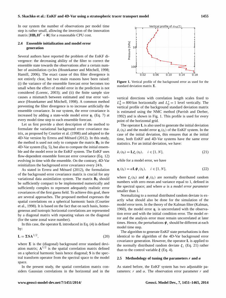
Fig. 1: Vertical profile of the background error as used for the standard deviation matrix Σ.

19

Figure 1. Vertical profile of the background error as used for thestandard deviation matrix6.

vertical directions with correlation length scales fixed toLh

0 = 800 km horizontally andLv0 = 1 level vertically. The

vertical profile of the background standard deviation matrixis estimated using the NMC method (Parrish and Derber,1992) and is shown in Fig.1. This profile is used for everypoint of the horizontal grid.

The operatorL is also used to generate the initial deviationx̃i(t0) and the model errorηi(tk) of the EnKF system. In thecase of the initial deviation, this ensures that at the initialtime, both EnKF and 4D-Var systems have the same errorstatistics. For an initial deviation, we have:

x̃i(t0) = Lζ i(t0), i ∈ [1,N ], (21)

while for a model error, we have

ηi(tk) = αLψ i(tk), i ∈ [1,N ], (22)

where ζ i(t0) and ψ i(tk) are normally distributed randomnumbers with zero mean and variance equal to 1, defined inthe spectral space; and whereα is a model error parametersmaller than 1.

Normalizing to a normal distributed random deviate is ex-actly what should also be done for the simulation of themodel error term. In the theory of the Kalman filter (Kalman,1960), the model errorηi is uncorrelated with the observa-tion error and with the initial condition error. The model er-ror and the analysis error must remain uncorrelated at latertimes. Hence, the perturbationsψ i should be different at eachmodel time step.

The algorithm to generate EnKF state perturbations is thenidentical to the algorithm of the 4D-Var background errorcovariance generation. However, the operatorL is applied tothe normally distributed random deviateζ i (Eq. 21) ratherthan to the control variableξ (Eq.4).

2.5 Methodology of tuning the parametersr and α

As stated before, the EnKF system has two adjustable pa-rameters:r and α. The observation error parameterr and



the model error parameterα are adjusted statistically usinga χ2 diagnostic introduced byMénard and Chang(2000)for the Kalman filter. This diagnostic compares the inno-vation vectord with the innovation covariance matrixS=

HBeHT+R (Eq.16) using a Mahalanobis norm (Talagrand,

2010). Specifically, at every analysis time stepk, the value ofχ2

k is computed as follows:

χ2k = dT

k S−1k dk. (23)

An assimilation system is said to be optimal when〈χ2k 〉 is

equal to the number of observationsmk at time tk where〈〉

denote the statistical expectation. Since the number of ob-servations per time step is relatively large, i.e. about 1100 inour case, we can approximate〈χ2

k 〉 by a realization ofχ2k for

a given set of observed values (i.e. for a realization of theobservation error).

As shown byMénard and Chang(2000), modifying themodel error parameter changes the trend (or slope) ofχ2

k overtime, while modifying the observational error parameterr

changes the mean value ofχ2k . Since these two parameters

have distinguishable effects on the time series ofχ2k (mean

and trend), they can be tuned separately, as summarized byKhattatov et al.(2000):

1. Run the assimilation system and monitorχ2k /mk. If its

value increases (decreases) consistently with time, in-crease (decrease)α. This procedure is repeated until themean value ofχ2

k /mk does not show a trend in its timeseries.

2. If the average value ofχ2k /mk is larger (smaller) than

1, increase (decrease) the observation error scaling fac-tor r.

3 Experimental set-up

3.1 Observations

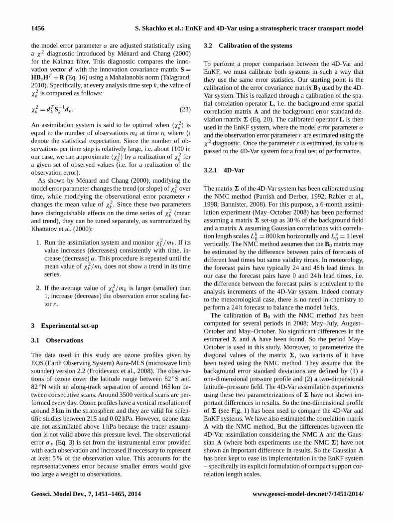
The data used in this study are ozone profiles given byEOS (Earth Observing System) Aura-MLS (microwave limbsounder) version 2.2 (Froidevaux et al., 2008). The observa-tions of ozone cover the latitude range between 82◦S and82◦N with an along-track separation of around 165 km be-tween consecutive scans. Around 3500 vertical scans are per-formed every day. Ozone profiles have a vertical resolution ofaround 3 km in the stratosphere and they are valid for scien-tific studies between 215 and 0.02 hPa. However, ozone dataare not assimilated above 1 hPa because the tracer assump-tion is not valid above this pressure level. The observationalerrorσ y (Eq. 3) is set from the instrumental error providedwith each observation and increased if necessary to representat least 5 % of the observation value. This accounts for therepresentativeness error because smaller errors would givetoo large a weight to observations.

3.2 Calibration of the systems

To perform a proper comparison between the 4D-Var andEnKF, we must calibrate both systems in such a way thatthey use the same error statistics. Our starting point is thecalibration of the error covariance matrixB0 used by the 4D-Var system. This is realized through a calibration of the spa-tial correlation operatorL , i.e. the background error spatialcorrelation matrix3 and the background error standard de-viation matrix6 (Eq. 20). The calibrated operatorL is thenused in the EnKF system, where the model error parameterα

and the observation error parameterr are estimated using theχ2 diagnostic. Once the parameterr is estimated, its value ispassed to the 4D-Var system for a final test of performance.

3.2.1 4D-Var

The matrix6 of the 4D-Var system has been calibrated usingthe NMC method (Parrish and Derber, 1992; Rabier et al.,1998; Bannister, 2008). For this purpose, a 6-month assimi-lation experiment (May–October 2008) has been performedassuming a matrix6 set-up as 30 % of the background fieldand a matrix3 assuming Gaussian correlations with correla-tion length scalesLh

0 = 800 km horizontally andLv0 = 1 level

vertically. The NMC method assumes that theB0 matrix maybe estimated by the difference between pairs of forecasts ofdifferent lead times but same validity times. In meteorology,the forecast pairs have typically 24 and 48 h lead times. Inour case the forecast pairs have 0 and 24 h lead times, i.e.the difference between the forecast pairs is equivalent to theanalysis increments of the 4D-Var system. Indeed contraryto the meteorological case, there is no need in chemistry toperform a 24 h forecast to balance the model fields.

The calibration ofB0 with the NMC method has beencomputed for several periods in 2008: May–July, August–October and May–October. No significant differences in theestimated6 and3 have been found. So the period May–October is used in this study. Moreover, to parameterize thediagonal values of the matrix6, two variants of it havebeen tested using the NMC method. They assume that thebackground error standard deviations are defined by (1) aone-dimensional pressure profile and (2) a two-dimensionallatitude–pressure field. The 4D-Var assimilation experimentsusing these two parameterizations of6 have not shown im-portant differences in results. So the one-dimensional profileof 6 (see Fig.1) has been used to compare the 4D-Var andEnKF systems. We have also estimated the correlation matrix3 with the NMC method. But the differences between the4D-Var assimilation considering the NMC3 and the Gaus-sian3 (where both experiments use the NMC6) have notshown an important difference in results. So the Gaussian3

has been kept to ease its implementation in the EnKF system– specifically its explicit formulation of compact support cor-relation length scales.



3.2.2 EnKF

Once the matrices3 and6 are calibrated in the 4D-Var sys-tem, the resulting operatorL is passed to the EnKF system.As explained in Sect.2.3, the EnKF uses a Schur productwith a compact support correlation function as a localizationmethod. The use of Schur product reduces the resulting cor-relation length scales. In order to maintain the correlations ofthe EnKF analysis comparable to those of the 4D-Var system,a different setting of the correlation length scales is adoptedto generate the model error (Eq.22). Let C be a matrix re-sulting from the Schur product of two matricesA and B:C = A ◦ B. If the correlation length scales ofA andB are,respectivelyLA andLB , the correlation length scale ofC isgiven by (Gaspari and Cohn, 1999)

1

L2C

=1

L2A

+1

L2B

. (24)

In our case,LA corresponds to the correlation length scaleLloc of the compact support correlation functionρ andLB

corresponds to the correlation length scale of the forecast en-semble covariance matrixBe, denoted in the following byLe.Similarly, LC corresponds to the correlation length scale ofthe analysis ensemble covariance matrix, denoted in the fol-lowing by the effective correlation length scaleLeff. As wewould like to maintain theLeff equal to the Gaussian correla-tion length scales used in the 4D-Var (i.e.Lh

0 = 800 km andLv

0 = 1 level), we need to setLloc andLe such thatLeff = L0.First, reasonable values for the localized correlation lengthscales were chosen:Lh

loc = 2000 km andLvloc = 1.5. In this

configuration, the correlation length scales used to generatethe model error in the EnKF are defined byLh

e = 872 km andLv

e = 1.3 model level.The next step in the calibration of the EnKF is the tuning of

α andr using aχ2 diagnostic (see Sect.2.5). Figure2 showsthe time evolution ofχ2

k /mk for three EnKF runs. The firstrun assumedr = 1 andα = 0, resulting inχ2

k /mk at ∼ 2.8initially and growing quickly during the following days. Themodel error parameterα was then adjusted by trial and erroruntil the time series ofχ2

k /mk displayed no trend, a conditionmet by a run usingα = 0.025. This second run still resultedin a too-largeχ2

k /mk, around 3. A second series of trial anderror adjustments for the observation error parameterr ledto the final run for the EnKF calibration: settingr = 1.65 re-sulted in analyses withχ2

k /mk close to 1.Figure 3 displays the observation-minus-forecast (OmF)

statistics, biases and standard deviations with respect to theassimilated MLS data, for these three EnKF experimentswith [α = 0, r = 1], [α = 0.025, r = 1] and [α = 0.025, r =

1.65]. A clear improvement is found after the tuning ofα, i.e.the presence of the model error term is essential for the EnKFto function properly. The impact of the tuning ofr is not sovisibly marked; however, the final EnKF experiment usingα and r parameters both tuned shows systematically betterresults than the experiment where onlyα is tuned. Overall,

01/05 01/07 01/09 01/11 01/010

1

2

3

4

5

6<χ2/m>

[α=0, r=1][α=0.025, r=1][α=0.025, r=1.65]

Fig. 2:⟨χ2/m

⟩evolution for the EnKF experiments using [α= 0, r= 1] (orange dashed line), [α= 0.04, r= 1] (green

dashed), and [α= 0.04, r= 1.6] (red solid). for the period from 00 UTC on 1 May 2008 to 00 UTC on 1 January 2009.

20

Figure 2.⟨χ2/m

⟩evolution for the EnKF experiments using[α =

0, r = 1] (orange dashed line),[α = 0.04, r = 1] (green dashed) and[α = 0.04, r = 1.6] (red solid) for the period from 00:00 UTC on1 May 2008 to 00:00 UTC on 1 January 2009.

this illustrates an important sensitivity of the EnKF to theadjustable error parameters.

The value ofr = 1.65 has been passed to the 4D-Var sys-tem for a final experiment to ensure the use of common ob-servation error statistics. Note that no significant differencesin the OmF statistics have been found between the 4D-Varanalysis withr = 1 andr = 1.65 (not shown). Thus, whilethe 4D-Var requires important work to develop an adjoint op-erator, the tuning of error parameters does not require largeefforts in the context of stratospheric chemistry.

3.3 Numerical performance

We tried to configure the EnKF and 4D-Var systems to allowcomparable total CPU costs. Preliminary experiments withthe 4D-Var system show that the 4D-Var performs reason-ably well using about 20 iterations. Accounting for the ad-joint model integration in the 4D-Var, we have chosen forthe EnKF an ensemble size of 40 members.

In terms of numerical performance, the 4D-Var requiresabout 750 s on a single processor to integrate one assimila-tion window of 24 h. The EnKF algorithm consists of twoseparate phases: the ensemble propagation and the analysis(Eq. 19). The analysis phase of the EnKF requires 550 s toperform 48 analyses, covering the period of 24 h, (48 anal-yses correspond to the model time step of 0.5 h) and 500 sto propagate the ensemble during the same period on a sin-gle processor. The actual EnKF configuration allows solvingEq.19on multiple processors, which helps to gain an impor-tant wall clock time: the analysis phase requires 100 s on 16processors. Note that the computation of the Kalman gain inour EnKF is performed using Cholesky decomposition where



-20 -10 0 10 20

1

10

100

Bias [-90°,-60°]

[%]

Pre

ssur

e [h

Pa]

4 8 12 16 20 24

1

10

100

Std. Dev. [-90°,-60°]

[%]

Pre

ssur

e [h

Pa]

-20 -10 0 10 20

1

10

100

Bias [-60°,-30°]

[%]

4 8 12 16 20 24

1

10

100

Std. Dev. [-60°,-30°]

[%]

-20 -10 0 10 20

1

10

100

Bias [-30°,30°]

[%]

4 8 12 16 20 24

1

10

100

Std. Dev. [-30°,30°]

[%]

-20 -10 0 10 20

1

10

100

Bias [30°,60°]

[%]

4 8 12 16 20 24

1

10

100

Std. Dev. [30°,60°]

[%]

-20 -10 0 10 20

1

10

100

Bias [60°,90°]

[%]

4 8 12 16 20 24

1

10

100

Std. Dev. [60°,90°]

[%]

[a=0.025, r=1.65]

[a=0.025, r=1]

[a=0, r=1]

Fig. 3: OmF statistics, bias and standard deviation, with respect to the MLS data of the EnKF experiments using [α=

0, r = 1] (orange dashed line), [α= 0.025, r = 1] (green dashed), and [α= 0.025, r = 1.65] (red solid). for the

period from 1 May to 31 June 2008.

−10 −5 0 5 10

1

10

100

Bias [−90°,−60°]

[%]

Pre

ssur

e [h

Pa]

0 10 20 30 40 50

1

10

100

Std. Dev. [−90°,−60°]

[%]

Pre

ssur

e [h

Pa]

−10 −5 0 5 10

1

10

100

Bias [−60°,−30°]

[%]

0 10 20 30 40 50

1

10

100

Std. Dev. [−60°,−30°]

[%]

−10 −5 0 5 10

1

10

100

Bias [−30°,30°]

[%]

0 10 20 30 40 50

1

10

100

Std. Dev. [−30°,30°]

[%]

−10 −5 0 5 10

1

10

100

Bias [30°,60°]

[%]

0 10 20 30 40 50

1

10

100

Std. Dev. [30°,60°]

[%]

−10 −5 0 5 10

1

10

100

Bias [60°,90°]

[%]

0 10 20 30 40 50

1

10

100

Std. Dev. [60°,90°]

[%]

4D−VarEnKF

Fig. 4: OmF statistics for the EnKF (red lines) and the 4D-Var (blue lines) with respect to the assimilated EOS Aura-MLS

data for the period September-October 2008. Bias (top row) and standard deviation (bottom row) for 5 different latitudinal

bands. The green or red stars show the result of the Student- and Fisher-tests of significance on the 95% level (see text).

21

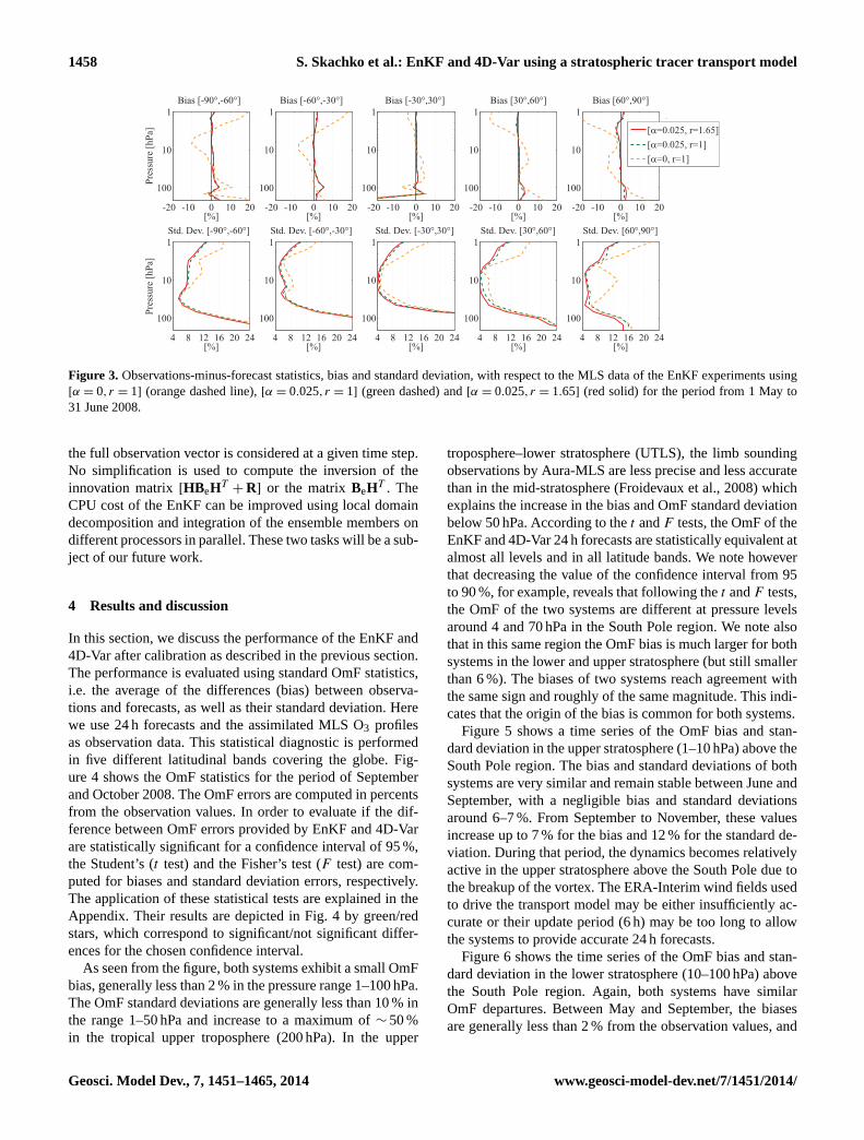
Figure 3. Observations-minus-forecast statistics, bias and standard deviation, with respect to the MLS data of the EnKF experiments using[α = 0, r = 1] (orange dashed line),[α = 0.025, r = 1] (green dashed) and[α = 0.025, r = 1.65] (red solid) for the period from 1 May to31 June 2008.

the full observation vector is considered at a given time step.No simplification is used to compute the inversion of theinnovation matrix[HBeHT

+ R] or the matrixBeHT . TheCPU cost of the EnKF can be improved using local domaindecomposition and integration of the ensemble members ondifferent processors in parallel. These two tasks will be a sub-ject of our future work.

4 Results and discussion

In this section, we discuss the performance of the EnKF and4D-Var after calibration as described in the previous section.The performance is evaluated using standard OmF statistics,i.e. the average of the differences (bias) between observa-tions and forecasts, as well as their standard deviation. Herewe use 24 h forecasts and the assimilated MLS O3 profilesas observation data. This statistical diagnostic is performedin five different latitudinal bands covering the globe. Fig-ure 4 shows the OmF statistics for the period of Septemberand October 2008. The OmF errors are computed in percentsfrom the observation values. In order to evaluate if the dif-ference between OmF errors provided by EnKF and 4D-Varare statistically significant for a confidence interval of 95 %,the Student’s (t test) and the Fisher’s test (F test) are com-puted for biases and standard deviation errors, respectively.The application of these statistical tests are explained in theAppendix. Their results are depicted in Fig.4 by green/redstars, which correspond to significant/not significant differ-ences for the chosen confidence interval.

As seen from the figure, both systems exhibit a small OmFbias, generally less than 2 % in the pressure range 1–100 hPa.The OmF standard deviations are generally less than 10 % inthe range 1–50 hPa and increase to a maximum of∼ 50 %in the tropical upper troposphere (200 hPa). In the upper

troposphere–lower stratosphere (UTLS), the limb soundingobservations by Aura-MLS are less precise and less accuratethan in the mid-stratosphere (Froidevaux et al., 2008) whichexplains the increase in the bias and OmF standard deviationbelow 50 hPa. According to thet andF tests, the OmF of theEnKF and 4D-Var 24 h forecasts are statistically equivalent atalmost all levels and in all latitude bands. We note howeverthat decreasing the value of the confidence interval from 95to 90 %, for example, reveals that following thet andF tests,the OmF of the two systems are different at pressure levelsaround 4 and 70 hPa in the South Pole region. We note alsothat in this same region the OmF bias is much larger for bothsystems in the lower and upper stratosphere (but still smallerthan 6 %). The biases of two systems reach agreement withthe same sign and roughly of the same magnitude. This indi-cates that the origin of the bias is common for both systems.

Figure 5 shows a time series of the OmF bias and stan-dard deviation in the upper stratosphere (1–10 hPa) above theSouth Pole region. The bias and standard deviations of bothsystems are very similar and remain stable between June andSeptember, with a negligible bias and standard deviationsaround 6–7 %. From September to November, these valuesincrease up to 7 % for the bias and 12 % for the standard de-viation. During that period, the dynamics becomes relativelyactive in the upper stratosphere above the South Pole due tothe breakup of the vortex. The ERA-Interim wind fields usedto drive the transport model may be either insufficiently ac-curate or their update period (6 h) may be too long to allowthe systems to provide accurate 24 h forecasts.

Figure6 shows the time series of the OmF bias and stan-dard deviation in the lower stratosphere (10–100 hPa) abovethe South Pole region. Again, both systems have similarOmF departures. Between May and September, the biasesare generally less than 2 % from the observation values, and



-20 -10 0 10 20

1

10

100

Bias [-90°,-60°]

[%]

Pre

ssur

e [h

Pa]

4 8 12 16 20 24

1

10

100

Std. Dev. [-90°,-60°]

[%]

Pre

ssur

e [h

Pa]

-20 -10 0 10 20

1

10

100

Bias [-60°,-30°]

[%]

4 8 12 16 20 24

1

10

100

Std. Dev. [-60°,-30°]

[%]

-20 -10 0 10 20

1

10

100

Bias [-30°,30°]

[%]

4 8 12 16 20 24

1

10

100

Std. Dev. [-30°,30°]

[%]

-20 -10 0 10 20

1

10

100

Bias [30°,60°]

[%]

4 8 12 16 20 24

1

10

100

Std. Dev. [30°,60°]

[%]

-20 -10 0 10 20

1

10

100

Bias [60°,90°]

[%]

4 8 12 16 20 24

1

10

100

Std. Dev. [60°,90°]

[%]

[a=0.025, r=1.65]

[a=0.025, r=1]

[a=0, r=1]

Fig. 3: OmF statistics, bias and standard deviation, with respect to the MLS data of the EnKF experiments using [α=

0, r = 1] (orange dashed line), [α= 0.025, r = 1] (green dashed), and [α= 0.025, r = 1.65] (red solid). for the

period from 1 May to 31 June 2008.

−10 −5 0 5 10

1

10

100

Bias [−90°,−60°]

[%]

Pre

ssur

e [h

Pa]

0 10 20 30 40 50

1

10

100

Std. Dev. [−90°,−60°]

[%]

Pre

ssur

e [h

Pa]

−10 −5 0 5 10

1

10

100

Bias [−60°,−30°]

[%]

0 10 20 30 40 50

1

10

100

Std. Dev. [−60°,−30°]

[%]

−10 −5 0 5 10

1

10

100

Bias [−30°,30°]

[%]

0 10 20 30 40 50

1

10

100

Std. Dev. [−30°,30°]

[%]

−10 −5 0 5 10

1

10

100

Bias [30°,60°]

[%]

0 10 20 30 40 50

1

10

100

Std. Dev. [30°,60°]

[%]

−10 −5 0 5 10

1

10

100

Bias [60°,90°]

[%]

0 10 20 30 40 50

1

10

100

Std. Dev. [60°,90°]

[%]

4D−VarEnKF

Fig. 4: OmF statistics for the EnKF (red lines) and the 4D-Var (blue lines) with respect to the assimilated EOS Aura-MLS

data for the period September-October 2008. Bias (top row) and standard deviation (bottom row) for 5 different latitudinal

bands. The green or red stars show the result of the Student- and Fisher-tests of significance on the 95% level (see text).

21

Figure 4. Observation-minus-forecast statistics for the EnKF (red lines) and the 4D-Var (blue lines) with respect to the assimilated EOS(earth observing system) Aura-MLS data for the period of September and October 2008. Bias (top row) and standard deviation (bottom row)for five different latitudinal bands. The green or red stars show the result of the Student’s and Fisher’s tests of significance on the 95 % level(see text).

01/05 01/06 01/07 01/08 01/09 01/10 01/11 01/12 01/01−10

−5

0

5

10OmF time series in [−90 °,−60°] and [1,10] hPa

Bia

s [%

]

01/05 01/06 01/07 01/08 01/09 01/10 01/11 01/12 01/010

5

10

15

20

Std

. Dev

. [%

]

4D−Var

EnKF

Fig. 5: OmF time series, bias (top row) and standard deviation (bottom row), for the EnKF (red lines) and the 4D-Var

(blue lines) with respect to the assimilated EOS Aura-MLS data between 1 and 10 hPa and between −90◦ and −60◦ for

the period May-December 2008.

22

Figure 5. Observations-minus-forecast time series, bias (top row)and standard deviation (bottom row), for the EnKF (red lines) andthe 4D-Var (blue lines) with respect to the assimilated EOS Aura-MLS data between 1 and 10 hPa and between−90 and−60◦ forthe period May–December 2008.

the standard deviations are less than 10 % until the end ofAugust. The standard deviations increase quickly during thefirst days of September and reach maximum values – around15–17 % – in mid-September, the 4D-Var providing valuesslightly lower than those from the EnKF. At the beginningof November, the standard deviations have decreased backto pre-September levels. In September, the bias of both ex-periments also slightly increases up to 4 % where 4D-Varshows again values slightly lower that those by the EnKF.In mid-October, the bias becomes negative but with values

01/05 01/06 01/07 01/08 01/09 01/10 01/11 01/12 01/01−10

−5

0

5

10OmF time series in [−90°,−60°] and [10,100] hPa

Bia

s [%

]

01/05 01/06 01/07 01/08 01/09 01/10 01/11 01/12 01/010

5

10

15

20

Std

. Dev

. [%

]

4D−Var

EnKF

Fig. 6: As Fig. 5 but between 10 and 100 hPa.

23

Figure 6. As Fig.5 but between 10 and 100 hPa.

lower than−2 %. Since the months of September and Octo-ber are precisely the period of photochemically driven ozonedestruction, we attribute these degradations in the OmF seriesto the absence of chemistry in our simplified model: duringthe ozone hole period, the tracer transport approximation isclearly not adequate. In this situation, the 4D-Var delivereda slightly better performance than the EnKF. This may bedue to the assimilation window of 24 h used by the 4D-Var,compared with the sequential assimilation of the EnKF.

Outside the ozone hole period/region and based onthe OmF statistics between MLS and the analysis, nosignificant differences have been found between thesystems. Observation-minus-forecast statistics have also



Figure 7. Ozone at 54.6 hPa (model level 22) from 4D-Var (left), EnKF (middle) and their absolute differences (right). The upper rowcorresponds to a snapshot on 15 September 2008 while the lower row corresponds to a monthly mean for the month of September 2008.

been computed against independent observations by En-visat/MIPAS (Michelson Interferometer for Passive Atmo-spheric Sounding) (Raspollini et al., 2013). Although theOmF statistics differ slightly, no statistical differences be-tween the EnKF and 4D-Var systems have been found ei-ther (not shown). Hence, the slightly different OmF statisticsare only due to the differences between the MLS and MIPASdata sets. We thus conclude that both systems are statisticallyequivalent in the observation space except during the ozonehole period, where the 4D-Var delivers analyses with slightlysmaller OmF departures than the EnKF.

However, individual analyses provided by the two systemscan exhibit larger differences than those given by OmF statis-tics. Figure7 (upper row) shows the ozone distribution at54.6 hPa on 15 September 2008 by both systems and theirdifferences. Although both analyses display similar patterns,they are clearly not identical. But looking at the monthlyaveraged maps (Fig.7, lower row) these difference becomesmall. Hence, while there are some differences between theanalyses by the two systems, these are not systematic and canbe attributed to noise in the analyses.

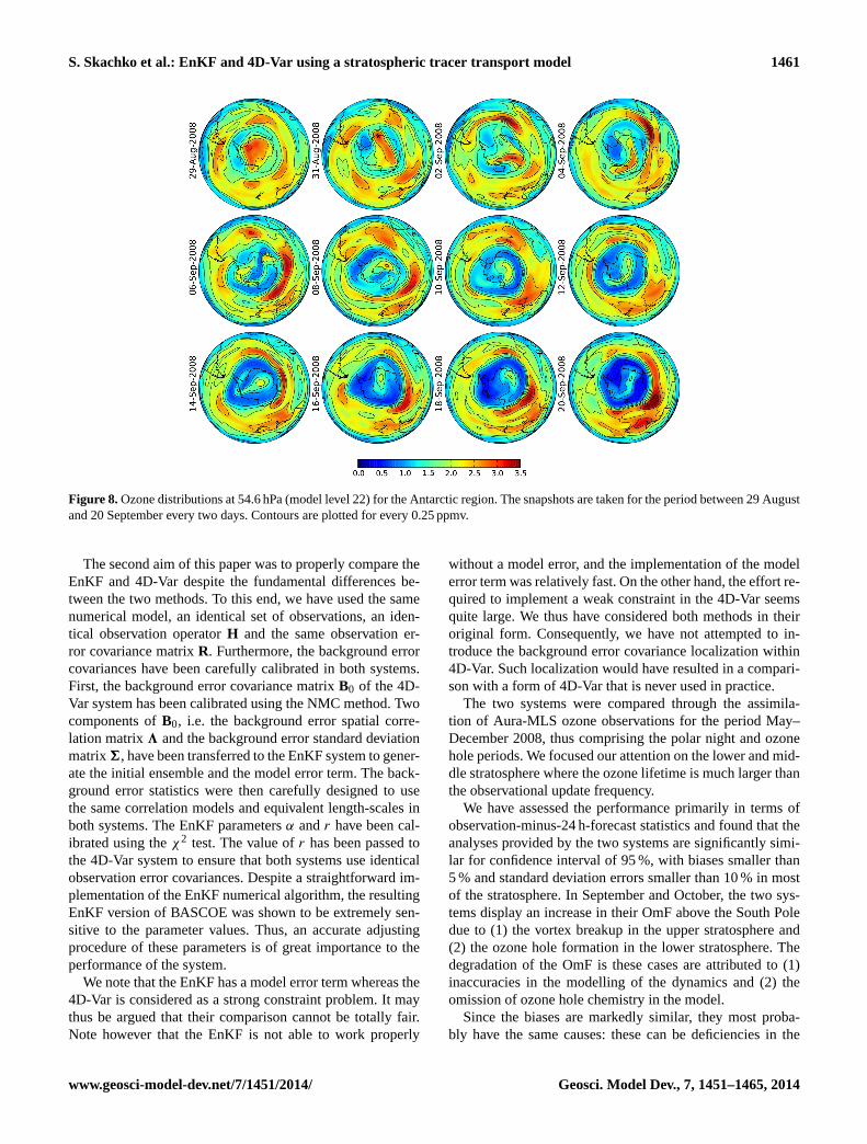
Finally, let us come back to the time series of theχ2 di-agnostic for the EnKF system (Fig.2). A small but sharp in-crease occurs during the first days of September. We attributethis jump to the onset of photochemically driven ozone de-pletion. Figure8 shows the formation of the ozone holethrough ozone analyses delivered by the EnKF system at54.6 hPa (model level 22) in the Southern Hemisphere from29 August to 20 September (one snapshot every two days).While it takes several days to see a clear ozone hole aboveAntarctica (even on 20 September ozone depletion is not

complete yet), ozone depletion started during the first daysof September, i.e. exactly during the sudden growth ofχ2. Ifthis growth is really due to a missing process in our model(in this case the ozone polar chemistry), thenχ2 may beused as a tool to monitor the model error. Note that althoughthe time series of the standard deviation in the OmF also in-creases during the formation of the ozone hole (see Fig.6),the growth in the standard deviation is smoother than dis-played by theχ2 and thus provides a less clear signal. Futurework will extend the comparison to the full BASCOE CTMincluding the ozone polar chemistry, and if our explanationis correct this sharp increase should disappear from theχ2

time series.

5 Conclusions

The first aim of this paper was to present the implementa-tion of the EnKF method in the BASCOE system. This sys-tem was originally based on 4D-Var, and our motivation wasto bypass the development and maintenance of an adjointmodel. The new EnKF version of BASCOE was developedaccounting for two adjustable parameters: the parameterα

controlling the model error term of the EnKF and the pa-rameterr controlling the observational error. These two pa-rameters have been adjusted based on the monitoring of aχ2

test measuring the misfit between the control variable and theobservations. In this study, we have turned off the chemistryin the CTM of BASCOE and have considered only ozonetransport. This configuration allowed considerably faster ex-ecution of both systems and a large number of assimilationexperiments.



Figure 8.Ozone distributions at 54.6 hPa (model level 22) for the Antarctic region. The snapshots are taken for the period between 29 Augustand 20 September every two days. Contours are plotted for every 0.25 ppmv.

The second aim of this paper was to properly compare theEnKF and 4D-Var despite the fundamental differences be-tween the two methods. To this end, we have used the samenumerical model, an identical set of observations, an iden-tical observation operatorH and the same observation er-ror covariance matrixR. Furthermore, the background errorcovariances have been carefully calibrated in both systems.First, the background error covariance matrixB0 of the 4D-Var system has been calibrated using the NMC method. Twocomponents ofB0, i.e. the background error spatial corre-lation matrix3 and the background error standard deviationmatrix6, have been transferred to the EnKF system to gener-ate the initial ensemble and the model error term. The back-ground error statistics were then carefully designed to usethe same correlation models and equivalent length-scales inboth systems. The EnKF parametersα andr have been cal-ibrated using theχ2 test. The value ofr has been passed tothe 4D-Var system to ensure that both systems use identicalobservation error covariances. Despite a straightforward im-plementation of the EnKF numerical algorithm, the resultingEnKF version of BASCOE was shown to be extremely sen-sitive to the parameter values. Thus, an accurate adjustingprocedure of these parameters is of great importance to theperformance of the system.

We note that the EnKF has a model error term whereas the4D-Var is considered as a strong constraint problem. It maythus be argued that their comparison cannot be totally fair.Note however that the EnKF is not able to work properly

without a model error, and the implementation of the modelerror term was relatively fast. On the other hand, the effort re-quired to implement a weak constraint in the 4D-Var seemsquite large. We thus have considered both methods in theiroriginal form. Consequently, we have not attempted to in-troduce the background error covariance localization within4D-Var. Such localization would have resulted in a compari-son with a form of 4D-Var that is never used in practice.

The two systems were compared through the assimila-tion of Aura-MLS ozone observations for the period May–December 2008, thus comprising the polar night and ozonehole periods. We focused our attention on the lower and mid-dle stratosphere where the ozone lifetime is much larger thanthe observational update frequency.

We have assessed the performance primarily in terms ofobservation-minus-24 h-forecast statistics and found that theanalyses provided by the two systems are significantly simi-lar for confidence interval of 95 %, with biases smaller than5 % and standard deviation errors smaller than 10 % in mostof the stratosphere. In September and October, the two sys-tems display an increase in their OmF above the South Poledue to (1) the vortex breakup in the upper stratosphere and(2) the ozone hole formation in the lower stratosphere. Thedegradation of the OmF is these cases are attributed to (1)inaccuracies in the modelling of the dynamics and (2) theomission of ozone hole chemistry in the model.

Since the biases are markedly similar, they most proba-bly have the same causes: these can be deficiencies in the



model and in the observation data set. The remarkably sim-ilar performance also shows that in the context of strato-spheric transport, the choice of the assimilation method canbe based on application-dependent factors, such as CPU costor the ability to generate an ensemble of forecasts.

The BASCOE 4D-Var system can provide analyses tak-ing stratospheric chemistry explicitly into account, in theforward as well as the adjoint model. The EnKF system

presented here accounts only for stratospheric transport, notchemistry. The application of the EnKF method to the full-chemistry model may require a careful tuning procedure foreach chemical species, a task that can be time consuming.Hence, an adaptive calibration procedure of the error covari-ances (similar toAnderson, 2009, or Li et al., 2009) shouldbe implemented. The implementation of EnKF with chem-istry is ongoing and will be reported in future studies.



Appendix A: Statistical tests to compare the OmF errors

A1 Student’s t test

We use the two-sample significance Student’st test (t test;see, e.g.Snedecor and Cochran, 1989) to compare two meanOmF residuals̄d(l) computed by the EnKF and the 4D-Var,where the bar denotes the time-averaged OmF residual valueat levell. This test is used in our case under the assumptionthat the two samples have the same size and variance. Thet statistics is computed at each levell as follows:

t (l) =d̄1(l) − d̄2(l)

Sd1d2(l)·

√2

n(l), (A1)

where n(l) is the size of the samples,Sd1d2(l) =√12(σ 2

1 + σ 22 ) is the grand or pooled standard deviation and

σ1(l) andσ2(l) are the OmF standard deviations for the EnKFand the 4D-Var at levell, respectively.

Then, for a given value of significance levelα (typicallyset to 5 %), the hypothesis that two means are statisticallyequal is rejected if

|t (l)| > T1−α/2,n(l), (A2)

whereTα,n(l) is a critical value oft (l) computed as the in-verse of the Student’st cumulative distribution function (cdf)for a givenα andn(l). The well knownt tables provide thevalues ofTα,n(l) only for small sample sizesn(l). In prac-tice, the Student’st cdf is easily computed by many statisticalpackages like SciPy, the Matlab statistical toolbox, etc.

A2 Fisher’s Test

The Fisher’sF test (Snedecor and Cochran, 1989) is used tocompare two OmF standard deviations and determine if theyare significantly different. For a two-tailed significance test itis supposed thatσ 2

1 6= σ 22 . TheF test statistics is computed

as at each levell as follows

f (l) =σ 2

1 (l)

σ 22 (l)

. (A3)

The more this ratio deviates from 1, the stronger the evidencefor unequal OmF standard deviations. The hypothesis that thetwo OmF standard deviations are equal is rejected if

f (l) > Fα/2,n(l), (A4)

or

f (l) < F1−α/2,n(l), (A5)

whereFα,n(l) is the critical value ofF distribution computedasF cumulative distribution function withn(l) degrees offreedom and a significance level ofα. TheF cdf can be com-puted using the same statistical packages as for thet cdf.



Acknowledgements.This research was financially supported atBIRA-IASB by the Belspo/ESA/PRODEX programme (PRODEXproject BACCHUS). Sergey Skachko wishes to thank LaurentBertino for his help in the numerical implementation of theinversion of the innovation matrix within the EnKF Kalman gain,as well as Mark Buehner, Takemasa Miyoshi, Emil Constantinescuand Saroja Polavarapu for helpful discussion on EnKF issues. Weare grateful to NASA JPL for providing EOS Aura-MLS data andto ECMWF for providing the ERA-Interim reanalysis.

Edited by: A. Sandu

References

Anderson, J. L.: Spatially and temporally varying adaptive covari-ance inflation for ensemble filters, Tellus A, 61, 72–83, 2009.

Bannister, R. N.: A review of forecast error covariance statistics inatmospheric variational data assimilation. I: Characteristics andmeasurements of forecast error covariances, Q. J. Roy. Meteorol.Soc., 134, 1951–1970, 2008.

Buehner, M., Houtekamer, P. L., Charette, C., Mitchell, H. L., andHe, B.: Intercomparison of Variational Data Assimilation and theEnsemble Kalman Filter for Global Deterministic NWP. Part I:Description and Single-Observation Experiments, Mon. WeatherRev., 138, 1550–1566, 2010a.

Buehner, M., Houtekamer, P. L., Charette, C., Mitchell, H. L., andHe, B.: Intercomparison of Variational Data Assimilation and theEnsemble Kalman Filter for Global Deterministic NWP. Part II:One-Month Experiments with Real Observations, Mon. WeatherRev., 138, 1567–1586, 2010b.

Constantinescu, E. M., Sandu, A., Chai, T., and Carmichael, G. R.:Ensemble-based chemical data assimilation. I: General approach,Q. J. Roy. Meteorol. Soc., 133, 1229–1243, 2007a.

Constantinescu, E. M., Sandu, A., Chai, T., and Carmichael, G. R.:Ensemble-based chemical data assimilation. II: Covariance lo-calization, Q. J. Roy. Meteorol. Soc., 133, 1245–1256, 2007b.

Courtier, P., Andersson, E., Heckley, W., Pailleux, J., Vasiljevic,D., Hamrud, M., Hollingsworth, A., Rabier, F., and Fisher, M.:The ECMWF implementation of three-dimensional variationalassimilation (3D-Var). I: Formulation, Q. J. Roy. Meteorol. Soc.,124, 1783–1807, 1998.

Dee, D. P., Uppala, S. M., Simmons, A. J., Berrisford, P., Poli,P., Kobayashi, S., Andrae, U., Balmaseda, M. A., Balsamo, G.,Bauer, P., Bechtold, P., Beljaars, A. C. M., van de Berg, L., Bid-lot, J., Bormann, N., Delsol, C., Dragani, R., Fuentes, M., Geer,A. J., Haimberger, L., Healy, S. B., Hersbach, H., Hólm, E. V.,Isaksen, L., Kållberg, P., Köhler, M., Matricardi, M., McNally,A. P., Monge-Sanz, B. M., Morcrette, J.-J., Park, B.-K., Peubey,C., de Rosnay, P., Tavolato, C., Thépaut, J.-N., and Vitart, F.: TheERA-Interim reanalysis: configuration and performance of thedata assimilation system, Q. J. Roy. Meteorol. Soc., 137, 553–597, 2011.

Elbern, H., Schwinger, J., and Botchorishvili, R.: Chemical stateestimation for the middle atmosphere by four-dimensional varia-tional data assimilation: System configuration, J. Geophys. Res.,115, D06302, doi:10.1029/2009JD011953, 2010.

Errera, Q. and Ménard, R.: Technical Note: Spectral representa-tion of spatial correlations in variational assimilation with gridpoint models and application to the Belgian Assimilation System

for Chemical Observations (BASCOE), Atmos. Chem. Phys., 12,10015–10031, doi:10.5194/acp-12-10015-2012, 2012.

Errera, Q., Daerden, F., Chabrillat, S., Lambert, J. C., Lahoz, W. A.,Viscardy, S., Bonjean, S., and Fonteyn, D.: 4D-Var assimilationof MIPAS chemical observations: ozone and nitrogen dioxideanalyses, Atmos. Chem. Phys., 8, 6169–6187, doi:10.5194/acp-8-6169-2008, 2008.

Evensen, G.: Sequential data assimilation with a nonlinear quasi-geostrophic model using Monte Carlo methods to forecast errorstatistics, J. Geophys. Res., 99, 10143–10162, 1994.

Evensen, G.: The Ensemble Kalman Filter: theoretical formula-tion and practical implementation, Ocean Dynam., 53, 343–367,2003.

Fertig, E. J., Hunt, B. R., Ott, E., and Szunyogh, I.: Assimilatingnon-local observations with a local ensemble Kalman filter, Tel-lus A, 59, 719–730, 2007.

Flemming, J., Inness, A., Flentje, H., Huijnen, V., Moinat, P.,Schultz, M. G., and Stein, O.: Coupling global chemistry trans-port models to ECMWF’s integrated forecast system, Geosci.Model Dev., 2, 253–265, doi:10.5194/gmd-2-253-2009, 2009.

Froidevaux, L., Jiang, Y. B., Lambert, A., Livesey, N. J., Read,W. G., Waters, J. W., Browell, E. V., Hair, J. W., Avery, M. A.,McGee, T. J., Twigg, L. W., Sumnicht, G. K., Jucks, K. W.,Margitan, J. J., Sen, B., Stachnik, R. A., Toon, G. C., Bernath,P. F., Boone, C. D., Walker, K. A., Filipiak, M. J., Harwood,R. S., Fuller, R. A., Manney, G. L., Schwartz, M. J., Daffer,W. H., Drouin, B. J., Cofield, R. E., Cuddy, D. T., Jarnot, R. F.,Knosp, B. W., Perun, V. S., Snyder, W. V., Stek, P. C., Thurstans,R. P., and Wagner, P. A.: Validation of Aura Microwave LimbSounder stratospheric ozone measurements, J. Geophys. Res.-Atmos., 113, D15S20, doi:10.1029/2007JD008771, 2008.

Gaspari, G. and Cohn, S. E.: Construction of correlation functionsin two and three dimensions, Q. J. Roy. Meteorol. Soc., 125, 723–757, 1999.

Hamill, T. M.: Ensemble-based atmospheric data assimilation,in: Predictability of Weather and Climate, edited by: Palmer,T. and Hagedorn, T., 124–156, Cambridge University Press,doi:10.1017/CBO9780511617652.007, 2006.

Hamill, T. M., Whitaker, J., and Snyder, C.: Distance-DependentFiltering of Background Error Covariance Estimates in an En-semble Kalman Filter, Mon. Weather Rev., 129, 2776–2790,2001.

Houtekamer, P. L. and Mitchell, H. L.: Data Assimilation Usingan Ensemble Kalman Filter Technique, Mon. Weather Rev., 126,796–811, 1998.

Houtekamer, P. L. and Mitchell, H. L.: A Sequential EnsembleKalman Filter for Atmospheric Data Assimilation, Mon. WeatherRev., 129, 123–137, 2001.

Kalman, R.: A new approach to linear filtering and prediction prob-lems, J. Basic Eng.-T. ASME, 82D, 35–45, 1960.

Kalnay, E., Li, H., Miyoshi, T., Yang, S.-C., and Ballabrera-Poy,J.: 4-D-Var or ensemble Kalman filter?, Tellus A, 59, 758–773,2007.

Khattatov, B. V., Gille, J. C., Lyjak, L. V., Brasseur, G. P., Dvortsov,V. L., Roche, A. E., and Waters, J. W.: Assimilation of photo-chemically active species and a case analysis of UARS data, J.Geophys. Res., 104, 18715–18737, 1999.

Khattatov, B. V., Lamarque, J.-F., Lyjak, L. V., Menard, R., Levelt,P., Tie, X., Brasseur, G. P., and Gille, J. C.: Assimilation of satel-


http://dx.doi.org/10.1029/2009JD011953

http://dx.doi.org/10.5194/acp-12-10015-2012



http://dx.doi.org/10.5194/gmd-2-253-2009

http://dx.doi.org/10.1029/2007JD008771

http://dx.doi.org/10.1017/CBO9780511617652.007


lite observations of long-lived chemical species in global chem-istry transport models, J. Geophys. Res., 105, 29135–29144,2000.

Lahoz, W. and Errera, Q.: Constituent Assimilation, in: Data As-similation: Making sense of observations, edited by: Lahoz, W.,Khattatov, B., and Ménard, R., 449 –490, Springer, 2010.

Li, H., Kalnay, E., Miyoshi, T., and Danforth, C.: Accounting formodel errors in ensemble data assimilation, Mon. Weather Rev.,137, 3407–3419, 2009.

Lin, S.-J. and Rood, R. B.: Multidimensional Flux-Form Semi-Lagrangian Transport Schemes, Mon. Weather Rev., 124, 2046–2070, 1996.

Liu, J., Fung, I., Kalnay, E., Kang, J.-S., Olsen, E. T., andChen, L.: Simultaneous assimilation of AIRS XCO2 and me-teorological observations in a carbon climate model withan ensemble Kalman filter, J. Geophys. Res., 117, D05309,doi:10.1029/2011JD016642, 2012.

Lorenc, A. C.: The potential of the ensemble Kalman filter for NWP– a comparison with 4D-Var, Q. J. Roy. Meteorol. Soc., 129,3183–3203, 2003.

Ménard, R. and Chang, L.-P.: Assimilation of Stratospheric Chem-ical Tracer Observations Using a Kalman Filter. Part II:χ2-Validated Results and Analysis of Variance and Correlation Dy-namics, Mon. Weather Rev., 128, 2672–2686, 2000.

Ménard, R. and Daley, R.: The application of Kalman smoother the-ory to the estimation of 4DVAR error statistics, Tellus A, 48,221–237, 1996.

Ménard, R., Cohn, S. E., Chang, L.-P., and Lyster, P. M.: Assim-ilation of Stratospheric Chemical Tracer Observations Using aKalman Filter. Part I: Formulation, Mon. Weather Rev., 128,2654–2671, 2000.

Miyazaki, K., Eskes, H. J., Sudo, K., Takigawa, M., van Weele, M.,and Boersma, K. F.: Simultaneous assimilation of satellite NO2,O3, CO, and HNO3 data for the analysis of tropospheric chemi-cal composition and emissions, Atmos. Chem. Phys., 12, 9545–9579, doi:10.5194/acp-12-9545-2012, 2012.

Miyoshi, T., Sato, Y., and Kadowaki, T.: Ensemble Kalman Fil-ter and 4D-Var Intercomparison with the Japanese OperationalGlobal Analysis and Prediction System, Mon. Weather Rev., 138,2846–2866, 2010.

Nakamura, T., Akiyoshi, H., Deushi, M., Miyazaki, K., Kobayashi,C., Shibata, K., and Iwasaki, T.: A multi-model comparisonof stratospheric ozone data assimilation based on an ensem-ble Kalman filter approach, J. Geophys. Res., 118, 3848–3868,doi:10.1002/jgrd.50338, 2013.

Parrish, D. and Derber, J. C.: The National Meteorological Center’sspectral statistical interpolation analysis system, Mon. WeatherRev., 120, 1747–1763, 1992.

Rabier, F., McNally, A., Andersson, E., Courtier, P., Undén, P.,Eyre, J., Hollingsworth, A., and Bouttier, F.: The ECMWF im-plementation of three-dimensional variational assimilation (3D-Var). II: Structure functions, Q. J. Roy. Meteorol. Soc., 124,1809–1829, doi:10.1002/qj.49712455003, 1998.

Raspollini, P., Carli, B., Carlotti, M., Ceccherini, S., Dehn, A.,Dinelli, B. M., Dudhia, A., Flaud, J.-M., López-Puertas, M.,Niro, F., Remedios, J. J., Ridolfi, M., Sembhi, H., Sgheri, L.,and von Clarmann, T.: Ten years of MIPAS measurements withESA Level 2 processor V6 – Part 1: Retrieval algorithm and di-agnostics of the products, Atmos. Meas. Tech., 6, 2419–2439,doi:10.5194/amt-6-2419-2013, 2013.

Sakov, P., Evensen, G., and Bertino, L.: Asynchronous data assimi-lation with the EnKF, Tellus A, 62, 24–29, 2010.

Sandu, A. and Chai, T.: Chemical Data Assimilation – AnOverview, Atmosphere, 2, 426–463, 2011.

Sekiyama, T. T., Deushi, M., and Miyoshi, T.: Operation-OrientedEnsemble Data Assimilation of Total Column Ozone, SOLA, 7,41–44, 2011.

Snedecor, G. and Cochran, W.: Statistical Methods, Iowa State Uni-versity Press, 8th Edn., 1989.

Talagrand, O.: Evaluation of Assimilation Algorithms, in: Data As-similation: Making sense of observations, edited by: Lahoz, W.,Khattatov, B., and Ménard, R., 217–240, Springer, 2010.

Talagrand, O. and Courtier, P.: Variational assimilation of meteoro-logical observations with the adjoint vorticity equation. I: The-ory, Q. J. Roy. Meteorol. Soc., 113, 1311–1328, 1987.

Wu, L., Mallet, V., Bocquet, M., and Sportisse, B.: A comparisonstudy of data assimilation algorithms for ozone forecasts, J. Geo-phys. Res., 113, D20310, doi:10.1029/2008JD009991, 2008.


http://dx.doi.org/10.1029/2011JD016642


http://dx.doi.org/10.1002/jgrd.50338

http://dx.doi.org/10.1002/qj.49712455003

http://dx.doi.org/10.5194/amt-6-2419-2013

http://dx.doi.org/10.1029/2008JD009991

Documents

Comparison of the ensemble Kalman ﬁlter and 4D-Var ... · 2Air Quality Research Division, Environment Canada, Dorval, Canada Correspondence to: S. Skachko ... Data assimilation