The THORPEX observation impact inter-comparison experiment

Ronald Gelaro1, Rolf H. Langland2, Simon Pellerin3 and Ricardo Todling1

1Global Modeling and Assimilation Office, NASA Goddard Space Flight Center,

Greenbelt, MD, USA

2Naval Research Laboratory, Monterey, CA, USA

3Environment Canada, Dorval, Quebec, Canada

16 February 2010

Submitted for publication in Monthly Weather Review

Third THORPEX International Science Symposium Special Collection

Corresponding author: Ronald Gelaro, Global Modeling and Assimilation Office, NASA

Goddard Space Flight Center, Greenbelt, MD 20771, USA. Email: ron.gelaro@nasa.gov

Abstract

An experiment is being conducted to directly compare the impact of all assimilated obser-

vations on short-range forecast errors in different forecast systems using an adjoint-based

technique. The technique allows detailed comparison of observation impacts in terms of

data type, location, satellite sounding channel, or other relevant attribute. This paper

describes results for a “baseline” set of observations assimilated by three forecast systems

for the month of January 2007. Despite differences in the assimilation algorithms and

forecast models, the impacts of the major observation types are similar in each forecast

system in a global sense. However, regional details and other aspects of the results can

differ substantially. Large forecast error reductions are provided by satellite radiances,

geostationary satellite winds, radiosondes and commercial aircraft. Other observation

types provide smaller impacts individually, but their combined impact is significant.

Only a small majority of the total number of observations assimilated actually improves

the forecast, and most of the improvement comes from a large number of observations

that have relatively small individual impacts. Accounting for this behavior may be es-

pecially important when considering strategies for deploying adaptive (or “targeted”)

components of the observing system.

1. Introduction

The Observing System Research and Predictability Experiment (THORPEX) is a decade-

long World Weather Research Program (WWRP) to accelerate improvements in the

accuracy of one-day to two-week high-impact weather forecasts for the benefit of so-

ciety, the economy and the environment (Shapiro and Thorpe 2004). A primary goal

of THORPEX is to quantify the value of observations provided by the current global

atmospheric observing network in terms of their impact on numerical weather forecasts.

The information from observation impact evaluation studies is intended to provide guid-

ance for improved use of current observations, especially those provided by satellite

systems, and for the design and deployment of future observing systems that are most

likely to benefit numerical weather prediction. The latter may include temporary and

adaptive enhancements of the permanent observing network for the study and improved

prediction of specific phenomena such as tropical cyclones and severe winter storms.

With millions of observations assimilated every analysis cycle in modern forecast sys-

tems, and the number of available observations expected to increase significantly with

the launch of new hyper-spectral satellite instruments, quantifying the value provided by

these data has become a major challenge in atmospheric data assimilation. As a starting

point for achieving this goal, an experiment is being conducted under the auspices of the

THORPEX International Working Group on Data Assimilation and Observing Systems

(DAOS IWG) to directly compare the impact of observations in different operational,

or near-operational, forecast systems. The specific objective of the comparison experi-

ment is to provide, if possible, robust answers to the following questions: How similar or

different are the impacts of observations in one forecast system versus another? Which

observation types have the largest total impacts, and impacts per-observation? How do

observation impacts vary as a function of location, channel, or other relevant attribute

1

of a given data type?

Traditionally, the impacts of observations on numerical weather forecasts have been

measured mainly through observing system experiments (OSEs), in which observations

are removed from (or added to) a data assimilation system and the resulting forecasts

compared against ones produced using a control set (e.g., Kelly et al. 2007). OSEs

have been used successfully to provide a gross measure of the impact of observations

on forecasts at various lead times but, because of their expense (multiple executions of

the data assimilation system are required), usually involve a relatively small number

of independent experiments, each considering relatively large subsets of observations.

With this approach it is not practical to examine the impacts of, for example, individual

channels on a single satellite sounding instrument, let alone all observations assimilated

in a single analysis cycle.

In recent years, new approaches have been developed based on adjoint sensitivities with

respect to observations (Baker and Daley 2000) and related methods that can provide

more details about the impact of observations which may be useful to identify problems

with an observation or the way it is assimilated. The adjoint technique described in

Langland and Baker (2004, hereafter LB04) and in subsequent papers by Errico (2007)

and Gelaro et al. (2007, hereafter GZE07), has proven to be a flexible and computation-

ally efficient way to estimate the impacts of all assimilated observations on a selected

measure of short-range forecast error. Although subject to assumptions and limitations

inherent in the use of adjoint models, the technique efficiently estimates the impacts

of all observations simultaneously, and produces results that can be easily aggregated

by data type, location, channel, etc. The technique has gained popularity as a an al-

ternative or complement to traditional OSEs, and is currently used at several forecast

centers for experimentation or routine monitoring of the observing system (Langland

2

2005, Gelaro and Zhu 2009, Cardinali 2009). We use the adjoint technique to conduct

the comparison study described in this paper.

Experiments to compare the impacts of a “baseline” observation set, described in de-

tail in the sections that follow, were designed by members of the DAOS IWG from

the Naval Research Laboratory (NRL), NASA Global Modeling and Assimilation Of-

fice (GMAO), Environment Canada (EC), European Centre for Medium-range Weather

Forecasts (ECMWF) and Meteo France. This paper presents results from three forecast

systems: the Navy Operational Global Atmospheric Prediction System (NOGAPS) of

NRL, the Goddard Earth Observing System-version 5 (GEOS-5) of GMAO, and the

Global Deterministic Prediction System (GDPS) of EC. It is anticipated that follow-on

experiments will include contributions from other forecast centers.

Section 2 briefly summarizes the adjoint methodology for computing observation impact,

including variations of the measure proposed by LB04 applied to the nonlinear assim-

ilation schemes used at GMAO and EC. Section 3 describes the experimental design

and relevant details (similarities and differences) in each forecast system that affect the

results. Sections 4 and 5 describe the results of the comparison, quantifying the impacts

of the baseline observing system in various aspects and levels of detail. Conclusions are

presented in section 6.

2. Estimation of observation impact

The technique used to measure observation impact in this study is based on LB04. It

uses the adjoint of a data assimilation system (forecast model and analysis scheme) to

efficiently estimate the impact of individual observations on an energy-based measure of

3

forecast error

e = (xf − xt)TPTCP (xf − xt) , (1)

where xf is a forecast state, xt is a verification state (considered truth), C is a diagonal

matrix of weights that gives (1) units of energy per unit mass, P is a spatial projection

operator that measures e only within a specified region of interest and the superscript

T denotes the transpose operation. The measure of observation impact is taken to be

the difference in e, δe = e(xfa) − e(xf

b ), between forecasts initialized from an analysis

xa and corresponding background state xb, where this difference is due entirely to the

assimilation of the observations.

The data assimilation scheme used by NRL computes an analysis of the form

xa = xb + Kd , (2)

where K is a matrix that determines the scalar weight given to each observation and d

is the vector of observation-minus-background departures (innovations). As derived by

LB04, the observation impact for this scheme can be estimated by an inner-product

δeN = 〈KTg,d〉 , (3)

where KT is the adjoint of the analysis scheme and g is a vector in model space given

by

g = MT

b PTCP (xfb − xt) + MT

a PTCP (xfa − xt) , (4)

where MTb and MT

a represent the adjoint of the forecast model evaluated along the

trajectories xfb and xf

a , respectively. The subscript N in (3) is used to distinguish this

form of the impact calculation from augmented forms required for the EC and GMAO

schemes, described below.

With g given by (4), (3) provides a non-linear (essentially third-order) approximation

of δe in terms of d (Errico 2007). Its properties have been studied in detail by Errico

4

(2007) and GZE07. The impact of a particular subset of observations may be estimated

by summing only those terms in (3) involving the corresponding elements of d. The

computation of the weights KTg is done only once, however, based on the complete set

of observations. Thus, the impact of any subset of observations is determined with re-

spect to all other observations simultaneously. This contrasts with traditional observing

system experiments (OSEs) that estimate the forecast impact for subsets of observations

that are withheld from (or added to) the analysis in a series of separate experiments.

Gelaro and Zhu (2009) provide a detailed comparison of adjoint-based observation im-

pacts with those derived from OSEs.

In general, computation of the innovations requires an observation operator, H, that

relates the model state to the observations, y, such that d = y − H(x). In obtaining

(3), it has been assumed that H is either linear or a function of only xb. This is not

true in general, however, and, in practice, the analysis cost function is nonlinear and

difficult to minimize. The analysis schemes used by EC and GMAO solve this problem

by minimizing an approximate quadratic cost function defined by linearizing H around

the current state estimate, and then repeating the process until a satisfactory solution

is found. The repeated minimizations define the so-called outer loops of an incremental

variational data assimilation scheme (Courtier et al. 1994). In this case, the analysis

increment is not xa − xb = Kd as implied by (2), but rather, after loop j, the total

increment is

xj − xb = Kjdj + KjHj(xj−1 − xb) , (5)

where dj = y − H(xj−1) and Hj is the observation operator linearized around the

previous state estimate, xj−1 (Tremolet 2008). The effects of the outer loops in these

schemes can be important to the quality of the analysis, especially in four dimensional

variational (4D-Var) data assimilation in which H includes the forecast model. The

5

analyses for EC and GMAO in the present study are produced using two outer loops.

A consequence of this added complexity is that the impact of observations on the forecast

is no longer described by the simple expression (3). Tremolet (2008) showed that while

an exact computation of observation impact in a data assimilation system with multiple

outer loops requires second-order adjoints (and is therefore not feasible in a realistic

system), useful approximations are still possible. One such approximation is

δe =m∑

j=1

〈KT

j zj,dj〉 , (6)

where m is the number of outer loops, zj = HTj+1K

Tj+1zj+1 and zm = g. Observation

impact in the GMAO forecast system is computed as in (6) with m = 2, which yields

δeG = 〈KT

1 HT

2 KT

2 g,d1〉 + 〈KT

2 g,d2〉 . (7)

Note that the departures in the second (last) outer loop have weights that depend on

the minimization performed in this loop only. This term is similar in form to that in

(3) for the NRL scheme or an analysis produced using a single outer loop. In contrast,

the departures in the first (previous) outer loop(s) have weights that depend on the

minimizations performed in the current and successive outer loop(s).

Observation impact in the EC forecast system is computed using a variation of (7), also

discussed by Tremolet (2008), of the form

δeE = 〈KT

2 g,d1〉 . (8)

In this case, the operators linearized about the (more accurate) solution from the sec-

ond minimization are used in conjunction with the (larger) departures from the first

minimization. A systematic comparison of the approximations (7) and (8) is beyond

the scope of the present study, especially given the fact that observation impact in a

nonlinear data assimilation system is somewhat difficult to interpret precisely. However,

6

results in later sections show that both approximations provide reasonable estimates of

observation impact, with accuracy comparable to that of (3) used in the NRL forecast

system.

3. Experimental design

The methodology described in section 2 is used to examine the impact of observations on

24-hr forecasts from various analysis times during January 2007. The results reported

here are for a baseline set of assimilated observations, defined as those observation types

used in common by EC, GMAO and NRL during the experimental period. Satellite ob-

servations in the baseline set include radiances from three AMSU-A instruments (NOAA-

15, -16 and -18, channels 4–11 only), upper-air wind vectors (atmospheric motion vec-

tors) from geostationary and MODIS imagery, surface wind vectors from QuikSCAT,

and surface wind speed from SSM/I. In-situ observations include temperature, humid-

ity, wind and surface pressure from radiosondes and dropsondes, surface pressure from

land-based stations, temperature, humidity and wind from surface ships and buoys, and

temperature, humidity and wind from commercial aircraft. Other more-recent observa-

tion types, such as AIRS and IASI, are not included in this baseline experiment, but

will be considered in future comparisons.

In keeping with the narrow focus of the comparison, it was decided that each center

would use its usual assimilation algorithm, including data selection and quality control

procedures, error statistics and observation operators. Thus, for some observation types

there are differences in how data are selected in each forecast system, leading to consid-

erable differences in the numbers of observations used. For example, NRL assimilates a

larger number of satellite winds from geostationary satellites than either EC or GMAO,

while GMAO assimilates a larger number of AMSU-A radiances (see Fig. 4).

7

Despite the effort to use identical input observation subsets in each forecast system,

a discrepancy was discovered after the fact. Both GMAO and NRL assimilate SSM/I

wind speeds but not profiler winds, while EC does the opposite. As shown in section 4,

neither data type is found to have a significant overall impact on the forecasts, at least

in terms of the error measure used in the present study. Therefore, as a practical matter,

this discrepancy is ignored.

The GMAO and NRL analyses for the comparison experiments are produced using three-

dimensional variational (3D-Var) data assimilation with a 6-hr cycle. The EC analyses

are produced using 4D-Var with a 6-hr cycle. The assimilation systems are all run at

horizontal resolutions close to 0.5 deg, but differ slightly in resolution as a result of

the discretization of the forecast model in each system (described below). The vertical

resolutions of the systems differ more significantly. NOGAPS (NRL) has 30 levels and

a top pressure of 1 hPa. GEOS-5 (GMAO) has 72 levels and a top pressure of 0.01 hPa.

GDPS (EC) has 80 levels and a top pressure of 0.1 hPa. Nonlinear forecasts are produced

at the same resolution as the corresponding analyses and include parameterized moist

physical processes. NOGAPS is a spectral model with a triangular truncation at T239.

GEOS-5 uses a finite-volume dynamical core with a grid resolution of 0.5 deg in latitude

and 0.67 deg in longitude. GDPS is a grid point model with a resolution of 0.3 deg in

latitude and 0.45 deg in longitude.

The adjoint versions of the forecast models used in these experiments are run without

moist physics. The forecast measure (adjoint cost function) is defined as the dry total

energy from the surface to approximately 150 hPa over the global domain, based on

(1). The NOGAPS adjoint model is run at the same resolution as the nonlinear forecast

model. The GEOS-5 adjoint model is run at half the resolution of the nonlinear model, or

approximately 1.0 deg. The GDPS adjoint model is run at a resolution of approximately

8

1.5 deg. Separate tests, as well as the results shown later, indicate that these differences

do not affect the observation impact calculations significantly. The adjoint version of

the analysis scheme in each forecast system is run at the same resolution and uses the

same observations as its forward counterpart.

From a practical perspective, we note that the computational cost of producing the

adjoint-based observation impact information for these experiments is about the same

as rerunning the forward analysis and forecast model. The cost would increase if the

adjoint model included the full suite of moist physical processes used in the nonlinear

model.

4. Impact of the baseline observing system

In the baseline experiment, observation impacts are computed for the 24-h forecasts

initiated at every analysis time (00, 06, 12 and 18 UTC) during the month of January

2007, providing 124 sets of results for each forecast system. We begin the comparison of

results by quantifying the overall impact of the baseline observing system in NOGAPS,

GEOS-5 and GDPS, and examining the accuracy of the respective adjoint-based impact

estimates used in the remainder of the study. Fig. 1 shows, for each forecast system,

time series of the 24-h forecast error measures e(xfb ) and e(xf

a) for every analysis time1,

in addition to the “true” impact e(xfa)− e(xf

b ) computed as the exact difference of these

quantities in model space, and the corresponding adjoint-based estimate, δeN , δeG or

δeE .

We note first that e(xfa) < e(xf

b ) for all analysis times in all three forecast systems

1Missing values in the GDPS time series are due to a post-processing problem that does not affect

other figures in the paper.

9

indicating that assimilation of the complete set of baseline observations consistently

results in a more skillful 24-h forecast. The work done by the observations is similar

in NOGAPS and GEOS-5, with average error reductions of 2.69 J/kg and 2.73 J/kg,

respectively, as determined by this difference. The average error reduction for GDPS is

smaller, at 1.64 J/kg. On the one hand, the smaller value for GDPS is consistent with

the general expectation that 4D-Var produces a better analysis than 3D-Var, providing

a better background for the subsequent analysis, and thus requiring smaller corrections

by the observations (Tremolet 2008). On the other hand, the values of e(xfb ) in GDPS

are not smaller than those in NOGAPS, which uses 3D-Var for these experiments.

The adjoint-based estimates provide a good approximation of the true error reduction

in all systems, recovering 78% and 73% of the total impact in NOGAPS and GEOS-

5, respectively, and 86% in GDPS, on average. These values are all in the range of

accuracy reported in earlier studies by LB04 and GZE07. The greater accuracy of the

adjoint-based estimate for GDPS is likely due to the use of the analysis trajectory to

evaluate both (versus only one) of the required gradients in (4). While there is no formal

justification for this substitution, empirical evidence shows that the relative error of this

form of the approximation is, on average, less than half that of the original third-order

one (GZE07).

The sawtooth pattern in the time series of e(xfb ) and e(xf

a) (and consequently in the

time series of observation impact) is due to the reduced accuracy of the background

forecasts initialized at 06 UTC and 18 UTC when there are fewer in-situ conventional

observations, followed by the comparatively large reduction of error in the corresponding

analyses at 12 UTC and 00 UTC when a much-larger number of conventional observa-

tions are present. The somewhat larger values of e(xfb ) and e(xf

a) overall in GEOS-5 may

indicate a sub-optimal use of the baseline set of observations, which excludes more than

10

half of the observations assimilated routinely in this forecast system, including radiance

measurements from AIRS, AMSU-B, HIRS and GOES sounders. Such a large reduction

in the number of observations might require, for example, a re-tuning of the background

error statistics to be consistent with the resulting change—presumably a reduction—in

the quality of the background forecast with the reduced set. No such re-tuning was done

for these experiments.

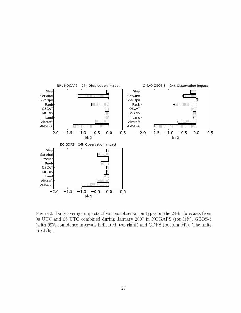
The results in Fig. 1 provide a context for further comparison of observation impacts in

the three forecast systems using the adjoint-based estimates. Fig. 2 displays the daily

average impacts of the major categories of observations in the baseline set. Results are

shown for the 00 UTC and 06 UTC analysis times combined so as to minimize dif-

ferences between synoptic times with and without conventional observations, although

such differences may be of interest for future study. The observation types shown in-

clude ships and buoys (Ship), geostationary satellite winds (Satwind), radiosondes and

dropsondes (Raob), QuikSCAT winds (QSCAT), MODIS satellite winds (MODIS), land

surface-pressure observations (Land), commercial aircraft (Aircraft) and AMSU-A radi-

ances (AMSU-A). Note that results are also shown for SSM/I winds speeds (SSMIspd)

in NOGAPS and GEOS-5 as opposed to profiler winds (Profiler) in GDPS, but that both

observation types have the smallest overall impact in the respective forecast systems.

In all three forecast systems, the largest total impact for this baseline set of observa-

tions is provided by AMSU-A radiances. Large impacts are also provided by geosta-

tionary satellite winds, radiosondes, and commercial aircraft. The dominance of these

four observation types appears to be a robust result, indicating that they are a critical

component of the global atmospheric observing network (the absence of other more cur-

rent observing systems notwithstanding). The remaining observation types—ship and

land surface, MODIS, and QuikSCAT—provide smaller impacts individually, but their

11

combined impact is significant in all forecast systems.

Radiosondes and AMSU-A radiances have noticeably smaller impact in GDPS than in

either NOGAPS or GEOS-5. These differences account for most of the smaller overall

impact of the baseline observing system in GDPS evident here and in Fig. 1. Other

notable differences between forecast systems include a much larger beneficial impact

from geostationary satellite winds in NOGAPS as compared with GEOS-5 or GDPS,

and a small non-beneficial impact from SSM/I wind speeds in GEOS-5. The latter is due

to a known deficiency in the procedure currently used to estimate the near-surface wind

speed from the model background state in that system, which introduces a significant

low bias in the departures at some midlatitude locations (Gelaro and Zhu 2009).

Plotted with the GEOS-5 results in Fig. 2 are the 99% confidence intervals based on a

t-statistic; the data required for this calculation were not available for NOGAPS and

GDPS. The range of uncertainty is small for all data types shown, reflecting the large

number of observations assimilated during the month (Fig. 4). Even the small overall

impacts from, say, SSM/I wind speeds or land surface observations in GEOS-5 appear

robust in terms of both amplitude and sign. Of course, these confidence intervals do not

reflect uncertainties due to errors in the adjoint approximation itself.

Figs. 3 and 4 show the impact per-observation (normalized impact) and total monthly

observation counts, respectively, in each forecast system for the same major observation

categories and synoptic times as in Fig. 2. The impact per-observation differs more

substantially between forecast systems than the average total impacts in Fig. 2, although

several common features are evident. Surface ship observations, which have small impact

overall, have one of the largest impacts per-observation. These observations are few in

number but are typically located in areas where there are few other in-situ data. The

12

value for these data in GDPS is 17 × 10−6 J/kg, which exceeds the scale in Fig. 3.

AMSU-A radiances, which have large overall impact (Fig. 2), have relatively small impact

per-observation in all forecast systems. This difference is most pronounced in GEOS-5,

which assimilates far more of these observations than any other data type in the baseline

set and, for example, more than twice the number assimilated in NOGAPS. Radiosondes

(plus dropsondes) have large impact per-observation as well as large overall impact in all

forecast systems. These observations are relatively numerous, but have high accuracy

and thus tend to be given significant weight in the analyses. MODIS winds have a large

impact per-observation in NOGAPS, especially compared to GEOS-5, which also has a

much smaller impact per-observation from land surface pressure observations than either

NOGAPS or GDPS.

The impact per-observation is smallest overall in GEOS-5, which assimilates a larger

number of most observation types. For example, roughly three times as many MODIS

wind observations are assimilated in GEOS-5 as in either NOGAPS or GDPS, with

comparable total impact (Fig. 2) but much smaller impact per-observation. The non-

beneficial impact of SSM/I wind speeds in GEOS-5 is also evident in Fig. 3. This is

likely due to the relatively small number of these observations overall and their location

over oceanic regions where there may be few other low-level wind data.

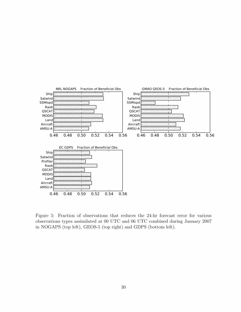
While the combined impact of the observations improves the forecast in all cases, there

is, in fact, a significant non-zero probability that individual observations, regardless of

data quality, can degrade a forecast. This is because data assimilation is fundamentally

a statistical problem dealing with unknown realizations of errors whose statistics are

only approximately known (Tarantola 1987). Fig. 5 shows, for each forecast system and

observation type, the fraction of observations assimilated at 00 and 06 UTC that reduces

13

the 24-h forecast error in the baseline experiments. It can be seen that, except for the

SSM/I wind speeds in GEOS-5 (which were shown to have a negative impact overall),

all observing systems are in the range of 50–54% beneficial. Thus, even those observing

systems that provide the largest overall benefit, such as AMSU-A radiances and ra-

diosondes, do so as a result of only a small majority of the total number of observations

assimilated, while the rest degrade the forecast. The fraction of beneficial observations

appears slightly higher overall in NOGAPS than in either GEOS-5 or GDPS, even if the

results for SSM/I wind speeds in GEOS-5 are disregarded.

It is difficult to place a precise upper bound on the fraction of observations that should

be expected to improve the analysis, especially in a operational data assimilation system.

Studies based on simple scalar data assimilation systems with perfectly specified error

statistics show that 60–65% of the observations lead to an improved analysis when the

background forecast and observations are of comparable accuracy (Ehrendorfer 2007, M.

Fisher 2007—personal communication), the latter condition being more or less represen-

tative of the current state of the art in operational forecasting. This is not to say that

comparable performance can be achieved in an operational data assimilation system by

marginal improvements in the background or observation error statistics alone. Note, for

example, that the fraction of beneficial observations is no larger in GDPS—and for some

observation types, smaller—than in NOGAPS or GEOS-5, even though the background

errors evolve implicitly through the assimilation window in 4D-Var (albeit over only a

6-hr period in these experiments).

5. Additional results for selected observation subsets

The results in section 4 quantify, in mostly bulk terms, the impact of whole observing

systems in NOGAPS, GEOS-5 and GDPS. For a given observing system, observation

14

impact can also be quantified as a function of measurement location, channel (in the

case of satellite radiances) or other attributes used to characterize an observation or

its representation in the assimilation system. In this section, we present more detailed

views of the impacts of selected components of the baseline observing system. As a

practical choice, we focus on observing systems that were shown in section 4 to provide

the largest overall benefits in all forecast systems, although similar figures can be easily

produced for other subsets of observations.

As is evident in Fig. 2, satellite radiance measurements have become a critical part of

the observing system for operational forecasting. Successful use of these data requires

careful quality control and bias correction procedures that are channel-specific. In addi-

tion, individual channels can degrade in quality or fail completely over time, making it

necessary to monitor these data on a per-channel basis. Hyper-spectral instruments such

as AIRS and IASI present an obvious challenge in this respect, because the large number

of channels makes evaluation and monitoring with traditional data-denial experiments

prohibitive from a computational standpoint

Fig. 6 compares the impact of individual AMSU-A channels in NOGAPS, GEOS-5 and

GDPS, averaged for the 00 UTC and 06 UTC analysis times combined as in previous

figures. The impacts vary from channel to channel but are generally similar in the

three forecast systems. Channels 5–7, which have weighting functions that peak in the

middle and upper troposphere between 600 and 200 hPa, provide large forecast error

reductions in all systems. The large impact from these channels is consistent with the

known high quality of the information provided by these channels (Mo 2007), but also

the fact that their weighting functions peak at levels where the largest errors tend to

occur as measured by an energy-based response function like the one used in this study

(Rabier et al. 1996). Differences in the relative magnitude of the impacts of AMSU-A

15

channels 5–7 in the three forecast systems are likely due to differences in data selection,

quality control or bias correction procedures. The smaller impacts of channels 5 and 6 in

GDPS appear to explain most of the smaller overall impact of AMSU-A in that system

as compared with NOGAPS and GEOS-5 (Fig. 2).

Channels 9–11, which have weighting functions that peak in the stratosphere above 100

hPa, have small impact, especially in NOGAPS and GEOS-5, as does channel 4, which

peaks in the lower troposphere near 850 hPa, in all forecast systems. The impact of

channel 9 is small compared with channels 5–7 in all forecast systems, but considerably

larger in GDPS than in NOGAPS or GEOS-5. Channel 8, which peaks near 150 hPa,

also has large impact in GEOS-5 and GDPS, but relatively small impact in NOGAPS.

An examination of the spatial variability of observation impact provided by the current

global observing system is another important objective of this comparison experiment.

Figs. 7–9 show, for NOGAPS, GEOS-5 and GDPS, respectively, the time-averaged spa-

tial distribution of observation impacts at 00 UTC and 06 UTC for three subsets of

observations: AMSU-A channel 7 radiances (top), radiosonde temperatures in the layer

450–550 hPa (middle), and satellite-derived zonal winds (geostationary and MODIS) in

the layer 250–350 hPa (bottom). The results in these figures represent average values

for observations that fall inside 2-degree bins in latitude and longitude. It is emphasized

that these figures depict the locations of observations and their impact on the global

forecast error measure, not the forecast errors themselves.

Large forecast error reductions occur in all forecast systems due to assimilation of AMSU-

A channel 7 radiances over much of the southern hemisphere between 30◦S and 70◦S,

as well as over the central North Pacific and western North Atlantic oceans. There are

also large error reductions from assimilation of these radiances over central China in

16

NOGAPS, and over western Asia in both GEOS-5 and GDPS. Interestingly, there are

also common areas of non-beneficial impact from these radiances in all forecast systems,

which occur over parts of India and north-central Canada near Hudson Bay. This could

be caused by land- or ice-surface contamination of the processed radiance observations,

and demonstrates the utility of the adjoint method for isolating possible problems with

the quality of the observations or the methodology used to assimilate them. Note also

that in many areas the impacts from this densely-spaced observation type are small in

magnitude (gray-shaded).

The impacts of radiosonde temperature observations are generally similar in all forecast

systems, with some notable differences including smaller overall values in GDPS as

expected from Fig. 2. Large error reductions occur in all three systems from assimilation

of these data over southeastern China and, to a lesser extent, Europe and the U.S., where

the impact of radiosonde observations may be reduced to some extent by large amounts

of data from commercial aircraft. There is also a more mixed pattern of beneficial and

non-beneficial impacts over Asia, although the range of values appears larger in GEOS-

5 and GDPS. The GEOS-5 and GDPS results also show mixed patterns of beneficial

and non-beneficial impacts from these data over Australia and the southeastern Pacific

Ocean, while in NOGAPS the impacts appear to be smaller but generally more beneficial

overall in these same regions.

The spatial patterns of observation impact from satellite winds differ more substantially

in the three forecast systems. The impacts are more uniformly beneficial in NOGAPS

than in GEOS-5 or GDPS. Except over the Arabian peninsula and, to a lesser extent, the

extreme southwestern Indian Ocean, there are substantial beneficial impacts from these

observations in most locations in NOGAPS, including the polar regions (from MODIS).

In GEOS-5 and GDPS, there are adjacent areas of large beneficial and non-beneficial

17

impacts over much of the southern midlatitudes, as well as over the northern Pacific. All

forecast systems show large beneficial impacts from these observations over the eastern

tropical Pacific and northeastern Pacific. Overall, however, the results point to possible

deficiencies in the use of these observations in GEOS-5 and GDPS as compared with

NOGAPS.

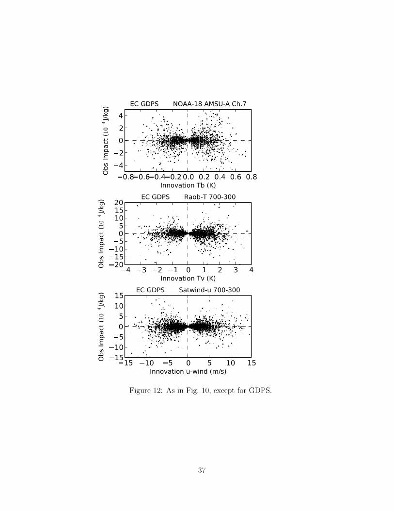
Figs. 10–12 illustrate how the adjoint method allows observation impact to be interpreted

in the context of other aspects of the assimilation process. Here we illustrate the relation

of observation impact to innovation value in the three forecast systems for the same

three observation types as in Figs. 7–9 (excluding MODIS satellite winds). For practical

reasons, results are shown for a single 24-h forecast initiated at 00UTC on 21 January but

are representative of other days during the study period. The axes are scaled differently

for each observation type, but the same scaling is used for all forecast systems. Two

aspects of these results appear to be fundamental to all forecast systems. The first is that

the numbers of observations providing beneficial impact (negative ordinate values) and

non-beneficial impact (positive ordinate values) are both large. This is consistent with

the results in Fig. 5, in which it was shown that only a small majority of the observations

provide a beneficial impact on average. The second aspect revealed by closer inspection

of Figs. 10–12 is that most of the total forecast error reduction comes from observations

with small to moderate sized innovations providing small to moderate sized reductions,

and not from outliers with very large values (although examples of the latter are evident

in all cases).

Figs. 10–12 also indicate differences in how observations are used in each assimilation

system, as well as possible deficiencies in the underlying assumptions made about the

inputs. The scatter diagrams for NOGAPS and GDPS form clear “bow-tie” patterns

with two distinct clusters corresponding to positive and negative innovation values, and

18

show relatively little impact coming from observations with innovations close to zero.

The impact values in GEOS-5 are more evenly distributed across the range of innovation

values, with a larger number of small impacts coming from observations with very small

innovation values.2 The innovations are smallest in GEOS-5 in an RMS sense for all

three observation types shown, especially for radiosonde temperatures at these levels.

The smaller impact per-observation for AMSU-A radiances in GEOS-5 is also evident

in these diagrams (cf. Fig. 3).

Asymmetries in the distribution of innovations about zero for some observation types

in Figs. 10–12 may indicate biases in the observations, background forecasts, or both.

The fact that the character of these asymmetries differs from one forecast system to

another suggests that they primarily reflect biases in the background forecasts, although

representativeness errors—introduced for example by interpolations associated with H—

also may play a role. Subject to this caveat, the NOGAPS background appears to

have a negative bias with respect to radiosonde temperatures in the middle troposphere

(Fig. 10, middle panel), which partially explains the larger innovations overall for this

observation type in NOGAPS. The GEOS-5 background appears to have a small positive

bias with respect to satellite winds in the upper troposphere (Fig. 11, lower panel). In

both cases, the more densely populated side of the diagram (with respect to the sign of

the innovation) also tends to have more observations with relatively large impact values.

The GDPS results exhibit almost no discernible biases overall in these figures, with the

possible exception of a slight negative bias with respect to the satellite wind observations

(Fig. 12, lower panel).

Note that the innovations for NOAA-18 satellite radiances exhibit no discernible biases

2Contrary to the impression given by Fig. 11, detailed views of the GEOS-5 results show that there

are no observations with zero-value innovations that provide non-zero impact.

19

in Figs. 10–12. Unlike the other observation types shown, these data undergo some

form of bias correction in most data assimilation systems, including the ones used in

this study. Because the bias is estimated and corrected with respect to the innovations

(that is, jointly with the model state variables), as opposed to just the observations, it

is not surprising that the distributions shown here appear unbiased. At the same time,

however, it is not possible to identify the actual source(s) of the bias detected this way

without additional information, such as independent observations (Dee 2005).

6. Conclusions

The first stage of an experiment to directly compare the impacts of observations in dif-

ferent forecast systems has been completed as part of a THORPEX initiative to quantify

the value of observations provided by the current global atmospheric observing network

in terms of their impact on numerical weather forecasts. An adjoint-based approach, first

proposed by Langland and Baker (2004), was used to compare the impact of observations

on 24-hr forecasts in three forecast systems: the Navy Operational Global Atmospheric

Prediction System (NOGAPS) of the Naval Research Laboratory (NRL), the Goddard

Earth Observing System-version 5 (GEOS-5) of the NASA Global Modeling and As-

similation Office (GMAO), and the Global Deterministic Prediction System (GDPS) of

Environment Canada (EC). Results were produced for a common baseline set of ob-

servations, including conventional observations of temperature, wind, surface pressure

and humidity, satellite-derived wind information from geostationary and polar-orbiting

satellites and radiances from three AMSU-A instruments. Unlike traditional observing

system experiments which, because of their expense, typically are used to measure only

the gross effects of (adding or removing) a few large subsets of observations on measures

of forecast skill, the adjoint method can provide more detailed information about the

20

impacts of all assimilated observations on a selected measure of short-range forecast er-

ror. The method is, however, subject to the usual approximations inherent in the use of

adjoint models; e.g., reliance on the tangent-linear assumption for error growth which,

for global-scale motions, becomes invalid beyond a couple days.

Despite substantial differences in the assimilation algorithms and forecast models used in

each system, it was found that the overall observation impacts are similar for most com-

ponents of the baseline observing system. The largest overall forecast error reductions

are provided by AMSU-A radiances, radiosondes and satellite winds, as well as aircraft

observations. These observing systems are clearly critical components of the current

atmospheric observing system, notwithstanding the fact that more-recent observation

types such as AIRS and IASI—which were not included in these experiments—also ap-

pear to provide substantial benefit to current numerical weather forecasts (Le Marshall

et al. 2006, Hilton et al. 2009). Other aspects of these results, such as the impact per-

observation for a given data type or the contributions from individual satellite sounding

channels, can vary significantly from one forecast system to another as a result of the

number of observations assimilated and, presumably, other characteristics of the data

handling and quality control procedures used.

It is, in general, difficult to determine the degree to which the impact of a given data type

reflects the quality of the observations assimilated as opposed to the methodology used

to assimilate them. Use of the adjoint technique in this comparison study allows some

interpretation of results in this regard. For example, examination of the spatial pattern

of observation impacts shows that all forecast systems make effective use of AMSU-

A radiances over the southern oceans and north Pacific, but that all show significant

non-beneficial impact from these observations over the Himalayan plateau and northern

Canada. The latter may point to a general deficiency in the use of microwave radiances

21

over specific (snow or ice covered) surface types. Results for other data types point

instead to strengths and weaknesses in individual forecast systems. For example, the

spatial pattern of observation impact from satellite winds was found to be highly variable

between forecast systems, with NOGAPS making more effective and uniformly beneficial

use of this data type than either GEOS-5 or GDPS.

Improving the use of the current global observing system, or planning for its evolution,

requires understanding not only the net effect of observations on the forecast but also

how these observations are used by the data assimilation system. It was found, for

example, that in all forecast systems only a small majority (less than 54%) of the total

number of observations assimilated actually reduces the global 24-h forecast error, while

the rest degrade it. With the large number of observations assimilated in each analysis

cycle, this small majority clearly is still enough to provide substantial overall benefit to

the forecast. At the same time, most of the total forecast error reduction comes from

a large number of observations with small to moderate-size innovations and forecast

impacts, and not from outliers with very large innovations, which do not contribute

much to the total impact. Both results point to the advantage of increasing the number

of observations assimilated as opposed to seeking a more limited set that produces only

the largest impacts, and to the potential importance of having some level of redundancy

between observing systems (see also Gelaro and Zhu 2009).

These same characteristics of how data are used by the assimilation system may have

ramifications for maximizing the benefit of temporary or adaptive enhancements of the

global observing system. In addition to deploying a limited number of in-situ obser-

vations in locally sensitive “targets of the day”, regional targeting of low-predictability

flow regimes on a continuous basis for periods of days to weeks (using, for example,

rapid-scan winds from geostationary satellites) may be an effective and practical means

22

of deploying supplemental observational resources. It is interesting to note that similar

conclusions were drawn from earlier studies on the deployment of targeted observations

(Morss 1999, Gelaro et al. 2000). This approach might also increase the effectiveness

of targeted observations into the medium-range, beyond the 1–3 day forecast lead time

typically used in the targeting of individual extreme events.

The results presented here should be viewed as only a first step in the ongoing work

within THORPEX to quantify and compare observation impacts in current forecast

systems. It is anticipated that future experiments will include more-recent observation

types, especially from hyper-spectral satellite sounding instruments, forecast metrics

that account explicitly for the effects of moisture and the impact of moisture observa-

tions, and results from other forecast systems.

Acknowledgments

The design of the baseline experiment benefitted from discussions with Pierre Gauthier

of Universite du Quebec a Montreal, Carla Cardinali of ECMWF, Stephane Laroche of

Environment Canada and Florence Rabier of Meteo-France. The authors thank Yan-

nick Tremolet of ECMWF for his work in developing the adjoint of the GSI analysis

scheme used in GEOS-5, and Ron Errico of GMAO for his helpful discussions about the

work. This work is supported by the NASA Modeling, Analysis and Prediction program

(MAP/04-0000-0080) and by the Naval Research Laboratory and the Office of Naval

Research, under Program Element 0602435N, Project Number BE-435-037.

23

References

Baker, N. and R. Daley, 2000: Observation and background adjoint sensitivity in theadaptive observation-targeting problem. Quart. J. Roy. Meteor. Soc., 126, 1431–1454.

Cardinali, C., 2009: Monitoring the observation impact on the short-range forecast.Quart. J. Roy. Meteor. Soc., 135, 239–250.

Courtier, P., J.-N. Thepaut and A. Hollingsworth, 1994: A strategy for operationalimplementation of 4D-Var, using an incremental approach. Quart. J. Roy. Meteor.

Soc., 120, 1367–1387.

Dee, D. P., 2005: Bias and data assimilation. Quart. J. Roy. Meteor. Soc., 131,3323–3343.

Ehrendorfer, M., 2007: A review of issues in ensemble-based Kalman filtering. Meteo-

rologische Zeitschrift, 16, 795–818.

Errico, R. M., 2007: Interpretation of an adjoint-derived observational impact measure.Tellus, 59A, 273–276.

Gelaro, R., C. A. Reynolds, R. H. Langland and G. D. Rohaly, 2000: A predictabil-ity study using geostationary satellite wind observations during NORPEX. Mon.

Wea. Rev., 128, 3789–3807.

Gelaro, R., Y. Zhu and R. M. Errico, 2007: Examination of various-order adjoint-basedapproximations of observation impact. Meteorologische Zeitschrift, 16, 685–692.

Gelaro, R. and Y. Zhu, 2009: Examination of observation impacts derived from ob-serving system experiments (OSEs) and adjoint models. Tellus 61A, 179–193.

Hilton, F., N. C. Atkinson, S. J. English and J. R. Eyre, 2009: Assimilation of IASI atthe Met Office and assessment of its impact through observing system experiments.Quart. J. Roy. Meteor. Soc., 135, 495–505.

Kelly, G., J.-N. Thepaut, R. Buizza and C. Cardinali, 2007: The value of observations.I: Data denial experiments for the Atlantic and Pacific. Quart. J. Roy. Meteor.

Soc., 133, 1803–1815.

Langland, R. H., 2005: Observation impact during the North Atlantic TReC - 2003.Mon. Wea. Rev., 133, 2297–2309.

Langland, R. H., and N. Baker, 2004: Estimation of observation impact using the NRLatmospheric variational data assimilation adjoint system. Tellus, 56, 189–201.

24

Le Marshall, J., J. Jung, J. Derber, M. Chahine, R. Treadon, S. Lord, M. Goldberg,W. Wolf, H. Liu, J. Joiner, J. Woollen, R. Todling, P. Van Delst, and Y. Tahara,2006: Improving global analysis and forecasting with AIRS. Bull. Amer. Meteor.

Soc., 87, 891–894.

Mo, T., 2007: Post-launch calibration of the NOAA-18 Advanced Microwave SoundingUnit-A. IEEE Trans. Geosci. Remote Sens., 45, 1928–1937.

Morss, R. E., 1999: Adaptive observations: Idealized sampling strategies for improvingnumerical weather prediction. Ph.D. thesis, Massachusetts Institute of Technology,225 pp. [Available from Dept. of Earth, Atmospheric and Planetary Sciences,Massachusetts Institute of Technology, Cambridge, MA 02139.]

Rabier, F., E. Klinker, P. Courtier and A. Hollingsworth, 1996: Sensitivity of forecasterrors to initial conditions. Quart. J. Roy. Meteor. Soc., 122, 121–150.

Shapiro, M. and A. Thorpe, 2004: THORPEX International Science Plan. WMO/TD-No. 1246, WWRP/THORPEX No. 2.

Tarantola, A., 1987. Inverse Problem Theory, Elsevier, Amsterdam.

Tremolet, Y., 2008: Computation of observation sensitivity and observation impact inincremental variational data assimilation. Tellus, 60A, 964–978.

25

1 6 11 16 21 26 31Date

�6�4�202468

101214

Energ

y (

J/kg

)

NRL NOGAPS 24h Fcst Error & Obs Impact

1 6 11 16 21 26 31Date

�6�4�202468

101214

Energ

y (

J/kg

)

GMAO GEOS-5 24h Fcst Error & Obs Impact

1 6 11 16 21 26 31Date

�6�4�202468

101214

Energ

y (

J/kg

)

EC GDPS 24h Fcst Error & Obs Impact

Figure 1: Time series of the 24-hr forecast error measures e(xfb ) (thick, positive values)

and e(xfa) (thin, positive values), total observation impact e(xf

a)−e(xfb ) (thick, negative

values), and corresponding adjoint-based estimate of total observation impact (thin,negative values) for each forecast system. Results are shown for all analysis times duringJanuary 2007 for NOGAPS (top left), GEOS-5 (top right) and GDPS (bottom left). Theunits are J/kg.

26

�2.0�1.5�1.0�0.5 0.0 0.5J/kg

AMSU-AAircraft

LandMODISQSCAT

Raob

SSMIspdSatwind

Ship

NRL NOGAPS 24h Observation Impact

�2.0�1.5�1.0�0.5 0.0 0.5J/kg

AMSU-AAircraft

LandMODISQSCAT

Raob

SSMIspdSatwind

Ship

GMAO GEOS-5 24h Observation Impact

�2.0�1.5�1.0�0.5 0.0 0.5J/kg

AMSU-AAircraft

LandMODISQSCAT

RaobProfiler

Satwind

Ship

EC GDPS 24h Observation Impact

Figure 2: Daily average impacts of various observation types on the 24-hr forecasts from00 UTC and 06 UTC combined during January 2007 in NOGAPS (top left), GEOS-5(with 99% confidence intervals indicated, top right) and GDPS (bottom left). The unitsare J/kg.

27

�15�12�9�6�3 0 31e-6 J/kg

AMSU-AAircraft

LandMODISQSCAT

Raob

SSMIspdSatwind

Ship

NRL NOGAPS 24h Impact Per-Observation

�15�12�9�6�3 0 31e-6 J/kg

AMSU-AAircraft

LandMODISQSCAT

Raob

SSMIspdSatwind

Ship

GMAO GEOS-5 24h Impact Per-Observation

�15�12�9�6�3 0 31e-6 J/kg

AMSU-AAircraft

LandMODISQSCAT

RaobProfiler

Satwind

Ship

EC GDPS 24h Impact Per-Observation

Figure 3: Impact per-observation for various observation types on the 24-hr forecastsfrom 00 UTC and 06 UTC combined during January 2007 in NOGAPS (top left), GEOS-5 (with 99% confidence intervals indicated, top right) and GDPS (bottom left). The unitsare 10−6 J/kg. The value for ships in the GDPS results is 17×10−6 J/kg, which exceedsthe scale.

28

0.0 0.2 0.4 0.6 0.8 1.0 1.2 1.41e7

AMSU-AAircraft

LandMODISQSCAT

Raob

SSMIspdSatwind

Ship

NRL NOGAPS Observation Count

0.0 0.2 0.4 0.6 0.8 1.0 1.2 1.41e7

AMSU-AAircraft

LandMODISQSCAT

Raob

SSMIspdSatwind

Ship

GMAO GEOS-5 Observation Count

0.0 0.2 0.4 0.6 0.8 1.0 1.2 1.41e7

AMSU-AAircraft

LandMODISQSCAT

RaobProfiler

Satwind

Ship

EC GDPS Observation Count

Figure 4: Total number of observations of various types assimilated at 00 UTC and 06UTC combined during January 2007 in NOGAPS (top left), GEOS-5 (top right) andGDPS (bottom left). The scale factor is 107.

29

0.46 0.48 0.50 0.52 0.54 0.56

AMSU-AAircraft

LandMODISQSCAT

Raob

SSMIspdSatwind

Ship

NRL NOGAPS Fraction of Beneficial Obs

0.46 0.48 0.50 0.52 0.54 0.56

AMSU-AAircraft

LandMODISQSCAT

Raob

SSMIspdSatwind

Ship

GMAO GEOS-5 Fraction of Beneficial Obs

0.46 0.48 0.50 0.52 0.54 0.56

AMSU-AAircraft

LandMODISQSCAT

RaobProfiler

Satwind

Ship

EC GDPS Fraction of Beneficial Obs

Figure 5: Fraction of observations that reduces the 24-hr forecast error for variousobservations types assimilated at 00 UTC and 06 UTC combined during January 2007in NOGAPS (top left), GEOS-5 (top right) and GDPS (bottom left).

30

�0.6�0.5�0.4�0.3�0.2�0.1 0.0 0.1J/kg

23456789

101112

AM

SU

-A C

hannel

NRL NOGAPS 24h Observation Impact

�0.6�0.5�0.4�0.3�0.2�0.1 0.0 0.1J/kg

23456789

101112

AM

SU

-A C

hannel

GMAO GEOS-5 24h Observation Impact

�0.6�0.5�0.4�0.3�0.2�0.1 0.0 0.1J/kg

23456789

101112

AM

SU

-A C

hannel

EC GDPS 24h Observation Impact

Figure 6: Daily average impacts of individual AMSU-A channels on the 24-hr forecastsfrom 00 UTC and 06 UTC combined during January 2007 in NOGAPS (top left), GEOS-5 (with 99% confidence intervals indicated, top right) and GDPS (bottom left). The unitsare J/kg.

31

Figure 7: Daily average impact of AMSU-A channel 7 radiances (top), radiosonde tem-peratures in the layer 450–550 hPa (middle), and satellite-derived zonal winds (geosta-tionary and MODIS) in the layer 250–350 hPa (bottom) on the NOGAPS 24-hr forecastsfrom 00 UTC and 06 UTC combined during January 2007. The units are 10−5 J/kg.Values are displayed for 2-deg bins in latitude and longitude.

32

Figure 8: As in Fig. 7, except for GEOS-5.

33

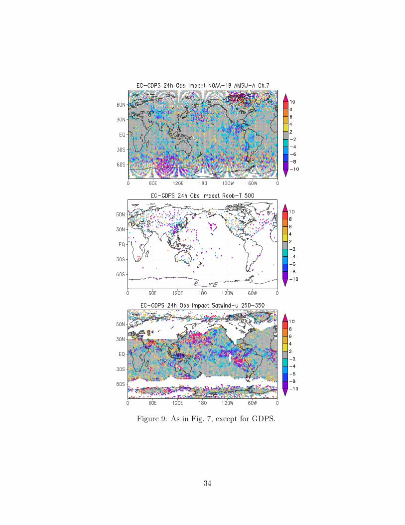
Figure 9: As in Fig. 7, except for GDPS.

34

�0.8�0.6�0.4�0.2 0.0 0.2 0.4 0.6 0.8Innovation Tb (K)

�4�202

4O

bs

Impact

(10

�4 J/kg) NRL NOGAPS NOAA-18 AMSU-A Ch.7

�4�3�2�1 0 1 2 3 4Innovation Tv (K)

�20

�15�10

�505101520

Obs

Impact

(10

�4 J/kg) NRL NOGAPS Raob-T 700-300

�15�10�5 0 5 10 15Innovation u-wind (m/s)

�15

�10

�50510

15

Obs

Impact

(10

�4 J/kg) NRL NOGAPS Satwind-u 700-300

Figure 10: Scatter diagram of observation impact versus innovation value for AMSU-Achannel 7 radiances (top), radiosonde temperatures in the layer 700–300 hPa (middle),and geostationary satellite zonal winds in the layer 700–300 hPa (bottom) for the NO-GAPS 24-h forecast initialized 00 UTC 21 January 2007.

35

�0.8�0.6�0.4�0.2 0.0 0.2 0.4 0.6 0.8Innovation Tb (K)

�4�202

4

Obs

Impact

(10

�4 J/kg) GMAO GEOS-5 NOAA-18 AMSU-A Ch.7

�4�3�2�1 0 1 2 3 4Innovation Tv (K)

�20�15�10�505101520

Obs

Impact

(10

�4 J/kg) GMAO GEOS-5 Raob-T 700-300

�15�10�5 0 5 10 15Innovation u-wind (m/s)

�15�10

�50510

15

Obs

Impact

(10

�4 J/kg) GMAO GEOS-5 Satwind-u 700-300

Figure 11: As in Fig. 10, except for GEOS-5.

36

�0.8�0.6�0.4�0.2 0.0 0.2 0.4 0.6 0.8Innovation Tb (K)

�4�202

4

Obs

Impact

(10

4 J/kg) EC GDPS NOAA-18 AMSU-A Ch.7

�4�3�2�1 0 1 2 3 4Innovation Tv (K)

�20�15�10�505101520

Obs

Impact

(10

4 J/kg) EC GDPS Raob-T 700-300

�15�10�5 0 5 10 15Innovation u-wind (m/s)

�15�10

�50510

15

Obs

Impact

(10

4 J/kg) EC GDPS Satwind-u 700-300

Figure 12: As in Fig. 10, except for GDPS.

37