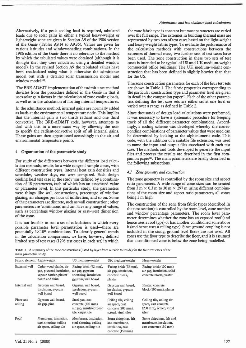
Proc. CIBSE A: Building Serv. Eng. Res. Technal. 21(2) 125-138 (2000) Printed in Great Britain B590

AJVC #13,235

Summary Calculation of design cooling loads is of critical concern to designers ofHVAC systems. The

work reported hi!:re has been carried out under a joint ASHRAE-CIBSE research project to compare design cooling calculation methods. Peak cooling :oads predicted by the ASHRAE heat balance method are compared with these predicted by a number of implementations of the admittance method

using different. window models. The r.esulrs presented show the general trends in overprediction or

under.predicti.ori of peak load. Particular attention is given to different window modelling practices.

The performance of the methods is explained in terms of some of the underlying assumptions in the

window models, and by reference to specific inter-model comparisons.

Comparison of peak load predictions and treatment of solar gains in the admittance and heat balance load calculation procedures

SJ Rees tt PhD CEng MCIBSE MASHRAE, JD Spitlertf: PhD PE MASHRAE, M J Holmes t CEng MCIBSE MASHRAE and P Haves t§ PhD CEng FCIBSE MASHRAE tDepartment of Civil and Building Engineering, Loughborough University, Loughborough, Leicestershire LEll 3TU, UK

:j:School of Mechanical & Aerospace Engineering, Oklahoma State University, Stillwater, OK 74074, USA §Lawrence Berkley National Laboratory, 1 Cyclotron Road, MS 90-31 1 1, Berkley, CA 94720, USA

Received 21 October 1999, in final form 21February 2000

List of symbols Absorption coefficient Effective front solar absorptance of the jth layer in the system

GcfP G.8 Solar gain to each node at hour 6 E<illf Total diffuse irradiance Ei Total solar irradiance

/in I

qd.ilf qD Se)S,

Direct irradiance Mean component of incident solar irradiance Fluctuating component of incident solar irradiance Inward flowing proportion of the absorbed radiation of the jth layer Diffuse solar gain per unit area of glazing Direct solar gain per unit area of glazing Mean solar gain factor for the environmental point and the air point

-�e , s. Alternating solar gain factor for the environmental point and the air point

SHGC Solar heat gain coefficient SHGC Normal solar heat gain coefficient T n Transmission coefficient T. Overall solar transmittance fJ Time (h); angle (deg) p Reflection coefficient r,.i G) Angularly dependent transmittance

Tref,n Normalised angularly dependent transmittance

Subscripts a Air point d.iff Diffuse I) Direct e Environmental point i Inner pane; inward direction n Normal o Outer pane

1 Introduction

The Chartered Institution of Building Services Engineers and· the America..11 Society of Heating Refrigeration and Air­Conditioning Engineers (ASHRAE) have published methods

© 2000 The Chartered Institution of Building Services Engineers

for design cooling and heating load calculations in their guides and handbooks for many years. Each organisation, working largely independently, has developed a somewhat different approach to design cooling load calculation proce­dures. Both CIBSE and ASHRAE have recognised that in the longer term both the efficiency and the reputation of the HV AC industry worldwide would be improved if common methods of performing key design calculations were adopted.

In 1996/97 the first joint CIBSE-ASHRAE research project 'Comparison of Cooling Load Calculation Procedures' (ASHRAE 942-RP, CIBSE 22/95) was initiated. It is the results of this project that are reported here. The aim of the work was to make inter-model comparisons between current UK and North American calculation procedures and to explain the differences in rhese results in terms of the underlying assump­tions of the methods. Further details of the results and the methods used in the project can be found in ASHRAE companion papers0.2J.

In recent years, both ASHRAE and CIBSE have been re-eval­uating and revising their load calculation procedures. In addi­tion, rhe Comite Europeen de Norma.Usation (CEN) is in the process of developing a standard approach to load calcula­tions. The draft CEN standard takes the form of a specifica­tion consisting of a set of heat balance equati.ons and a set of qualification tests against which particular computer codes can be evaluated. ASHRAE has a long history of developing and revising load calculation methods, RomineC3) gives a good summary Through to 1992. Recently ASHRAE has funded a research project entitled 'Advanced Methods for Calculating Peak Cooling Loads (875-RP)' the goal of which has been to replace the existing methods with two 'new' methods: the heat balance methodC4) and the radiant time series methodC5l.

The heat balance method is the most fundamental of all design load calculation methods and may be the method most under­standable by practising engineers, as it closely follows physical processes and has a minimum of mathematical abstraction. However, it does require the solution of several simultaneous equations. The second method, the radiant time series (RTS) method, is intended IO be simpler from a calculation

125

SJ Rees et a!.

standpoint and builds on the concepts of the existing transfer function (TFM) and total equivalent temperature difference/ time averaging (TETD/TA) methotls<6•7l.

CIBSE Guide Volume A: 1986<8' describes two load calculation methods: the environmental temperature nodal method, which deals with steady-state loads, and the admittance method <9•10>, which deals with fluctuating loads. Guide Volume A: 1999<11' contains two steady-state methods and two dynamic methods: one based on a detailed reference model, and one based on a simplified model (which is, in fact, the admittance method). The reference model consists of a perfor­mance specification, along with a list of features that must be included. Particular model equations or calculation methods are not specified, though it is difficlut to see how the require­ments could be met other than by a method based on explicit heat balances. To date, no public-domain design cooling load calculation computer codes have been developed that comply with the recommendations of CIBSE Guide A: 1999<11l.

In the work presented here, comparisons are made between the peak cooling load predictions of the new ASHRAE heat balance method<4l and one public-domain implementation of the admittance method<12•13l. Comparison with the predictions of the RTS method are reported in ASHRAE companion papers(l.Z>. A systematic comparison of the predictions of the methods is given along with an analysis of the sensitivity of the various parameters. The causes of the variations in predic­tions between the two methods are identified and are explained in terms of the approximations made. It is shown that some of the most significant differences arise from different window modelling practices. In view of this, further calculations have been made with an implementation of the admittance method using a detailed window model. These results and further findin� are discussed in section 9.

2 The calculation methods

Two design cooling load calculation methods are compared here. These are the 'heat balance method' (HBM) and the 'admittance method'. The main features of the methods are summarised below. A systematic comparison of the methods is given in Rees et al.<14l.

The heat balance method involves the solution of heat balance equations for each of the outside and inside zone surfaces, along with the zone air. This approach is similar to that of existing load and energy calculation codes such as T ARP<15> and BLAST<16l. Radiant and convective heat exchange are treated separately at both inside and outside surfaces, with interior radiant exchange being calculated using the mean radiant temperature/balance algorithm of Walton<17>. Tran­sient conduction through the zone fabric is dealt with using conduction transfer functions.

The approach taken in the admittance method is in one sense similar to that of the ASHRAE heat balance method in that the loads are found by solution of heat balance equations. However, the model used to represent the building zone, from which the heat balance equations are formulated, as well as the models used to treat the heat transfer processes, is rather simplified. A further significant feature of the admittance method is that the derivation of the method relies on the assumption that the boundary conditions (outside dry bulb, solar radiation, etc. ) fluctuate sinusoidally with a period of24 h.

126

-- ·-·----- - -- -----·

The calculation of cooling loads with the admittance method is a two-part process in that the mean components of the heat gains and loads are treated separately from the fluctuating components. The mean components are calculated using the CIBSE simplified steady-state model that is defined by a three node thermal network. The 'admittance procedure' defines how the fluctuating components of the loads and temperature differences are calculated.

Whereas the heat balance and RTS methods use the zone air temperature node as the point at which internal surfaces are convectively coupled, the admittance method relies on the concept of environmental temperature, which is used to calcu­late the combined radiant and convective heat exchange with the room surfaces. The concept of environmental temperature is similar to that of sol-air temperature used to define external surface heat transfer in that a combined radiant and convec­tive conductance is used. All the zone surfaces are linked to a common environmental temperature node at which a heat balance is calculated.

The heat balance method, being the most detailed of the methods, and being based to a greater extent on fundamental physical principles, has been used as a reference model in this work, against which the results of the admittance method have been compared. It should also be noted that cooling loads have been calculated on the basis of the room dry bulb temperature being maintained at a constant value.

3 Load calculation procedure implementations

In choosing the computer implementations to use in this comparison exercise, only implementations that were readily available and for which there was access to the source code were considered. Carrying out the large number of runs neces­sary for the study also made it a requirement that the imple­mentation could easily be adapted to run from standard input files. The implementation of the heat balance method used in this work was in the form of a Fortran 90 code developed for the 'Advanced Methods for Calculating Peak Cooling Loads (875-RP)' project.

There are a number of commercial implementations of the admittance method, but there is only one well-known code in the public domain: BRE-ADMIT<l3). This is, in fact, a set of programs written in BASIC that provide a user interface, generate solar data, calculate admittances, etc. from fabric thermal properties and perform the actual load/temperature calculation. The load/temperature calculation program (BRECALC) has been adapted to run from file input and send output to a file. The calculation of cooling loads in BRE­ADMIT is described by Danter<12l. It should be noted that the BRE-ADMIT code deviates in some of its details from the admittance method as defined in the Guide. This is particu­larly so in the case of the calculation of solar gains.

The CIBSE Guide A: l 986<8l prescribes two methods of calcu­lating solar gains using the admittance method. If an over­heating calculation is required, the total incident radiation is divided into its mean and fluctuating components. A solar gain factor and an alternating solar gain factor then multiply the mean and fluctuating components. These factors are constant and are defined for energy transfer to both the air and environmental temperature points. These solar gain factors are tabulated for various window/blind types in heavy and light-weight buildings located in London (Tables A8.2 and A8.6 of the 1986 edition of the C..uide).

Building Services Engineering Research and Technolo!!V

Alternatively, if a peak cooling load is required, tabulated loads due to solar gains in either a typical heavy-weight or light-weight zone are given in Section A9 of the 1986 version of the Guide (Tables A9.14 to A9.35). Values are given for various latitudes and window/shading combinations. In the 1986 edition of the Guide there is no reference to the method by which the tabulated values were obtained (although it is thought that they were calculated using a detailed window model). In the revised Section A9 the tabulated values have been recalculated using what is otherwise the admittance model but with a detailed solar transmission model and window model<11>.

The BRE-ADMIT implementation of the admittance method deviates from the procedure defined in the Guide in that it uses solar gain factors in the calculation of zone cooling loads, as well as in the calculation of floating internal temperatures.

In the admittance method, internal gains are normally added as loads at the environmental temperature node. This implies that the internal gain is two thirds radiant and one third convective. The BRE-ADMIT code, however, attempts to deal with this in a more exact way by allowing the user to specify the radiant-convective split of all internal gains. These gains are then apportioned accordingly to the air and environmental temperature points.

4 Organisation of the parametric study

For study of the differences between the different load calcu­lation methods, results for a wide range of sample zones, with different construction types, internal heat gain densities and schedules, weather days, etc. were compared. Each design cooling load test case in the study was defined by a combina­tion of 18 parameters, each of which has an associated value or parameter level. In ):his particular study, the parameters were things like wall constructions, percentage of window glazing, air changes per hour of infiltration, and so on. Some of the parameters are discrete, such as wall construction; other parameters are 'continuous' and can have any range of values, such as percentage window glazing or east-west dimension of the zone.

It is not feasible to run a set of calculations in which every possible parameter level permutation is used-there are potentially 5X1018 combinations. To identify general trends in the calculation comparisons, we have, however, defined limited sets of test cases (1296 test cases in each set) in which

Admittance and heat balance load calculations

the zone fabric type is constant but most parameters are varied over the full range. The extremes in building thermal mass are represented by two sets of test cases based on the light-weight and heavy-weight fabric types. To evaluate the performance of the calculation methods with constructions between the extremes of thermal mass, two further sets of test cases have been used. The zone construction in these two sets of test cases is intended to be typical of US and UK medium-weight commercial office buildings. The UK medium-weight con­struction that has been defined is slightly heavier than that for the US.

The zone construction parameters for each of the four test sets are shown in Table 1. The fabric properties corresponding to the particular construction type and parameter level are given in detail in the companion paper<1>. Each of the other parame­ters defining the test case sets are either set at one level or varied over a range as defined in Table 2.

Since thousands of design load calculations were performed, it was necessary to have a systematic procedure for keeping track of all the different parameter combinations. Accord­ingly, a coding scheme was developed whereby the corres­ponding combinations of parameter values that were used can be determined by looking at the alphanumeric code. This code, with the addition of a suitable file extension, was used to name the input and output files associated with each test case. The methods and tools developed to generate the input files and process the results are described in the first com­panion paper<!). The main parameters are briefly described in the following subsections.

4.1 Zone geometry and construction

The zone geometry is controlled by the room size and aspect ratio parameters. A wide range of zone sizes can be created from 3 m X 0.3 m to 30 m X 297 m using different combina­tions of the room size and aspect ratio parameters, all zones being 3 m high.

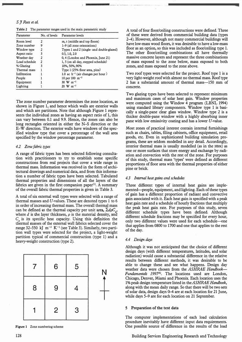
The construction of the zone from fabric types (described in the next section) is controlled by the room level, zone number and window percentage parameters. The room level para­meter determines whether the zone has an exposed roof (and hence uses a roof type) or has another conditioned zone above it (and hence uses a ceiling type). Since ground coupling is not included in the study, ground-level floors are not used. All zones use the floor type to describe the floor, and it is assumed that a conditioned zone is below the zone being modelled.

Table I A summary of the zone constructions (listed by layer from outside to inside) for the four test cases of the main parametric study

Fabric element Light-weight US medium-weight UK medium-weight Heavy-weight

External wall Cedar wood planks, air Facing brick (92 mm), Facing brick (75 mm), Facing brick (100 mm), gap, plywood insulation, air gap, gypsum air gap, insulation, air gap, insulation, solid vapour barrier, plaster sheathing, insulation concrete block, concrete block, plaster board and skim gypsum, wall board plaster

Internal wall Gypsum wall board, Gypsum wall board, Gypsum wall board, Plaster, concrete insulation, gypsum insulation, gypsum insulation, gypsum block (100 mm), plaster wall board wall board wall board

Floor and Gypsum wall board, Steel pan, cast Ceiling tile, ceiling Ceiling tile, ceiling air ceiling air gap, pine concrete (100 mm), air space, cast space, cast concrete

air gap, insulated floor concrete (200 mm), (200 mm), screed, vinyl tile, carpet tile screed, vinyl tiles tiles

Roof Membrane, insulation, Membrane, insulation, Stone chippings, felt Stone chippings, felt and steel sheeting, ceiling steel sheeting, ceiling and membrane, membrane, insulation, air space, ceiling tile air space, ceiling tile insulation, cast cast concrete (150 mm)

concrete (150 mm)

Vol. 21 No. 2 (2000) 127

SJ Rees et al.

Table 2 The parameter ranges used in the main parametric study

Parameter

Room level Zone number Window type Aspect ratio

Weather day Load schedule % Glazing Thermal mass Infiltration

People Equipment Lighting

No. oflevels Parameter levels

2 m, t (middle and top floors) 9 1-9 (all zone orientations)

2 Types 1 and 2 (single- and double-glazed) 3 0.5, 1.0, 2.0 2 0, 4 (London and Phoenix, June 21)

2 1, 5 (on all day, stepped schedule) 3 10%, 50%, 90%

Type 1 (25% floor area, pine)

1.0 ac h-1 (air changes per hour ) 10 per 100 m-2

30 W m-2 20 W m-2

The zone number parameter determines the zone location, as shown in Figure 1, and hence which walls are exterior walls and which are partitions. Note that although Figure 1 repre­sents the individual zones as having an aspect ratio of 1, this can vary between 0.1 and 9.9. Hence, the zones can also be long rectangles oriented in either the N-S direction or the E-W direction. The exterior walls have windows of the spec­ified window type that cover a percentage of the wall area specified by the window percentage parameter.

4.2 Zone fabric types

A range of fabric types has been selected following consulta­tion with practitioners to try to establish some specific constructions from real projects that cover a wide range in thermal mass. Information was received in the form of archi­tectural drawings and numerical data, and from this informa­tion a number of fabric types have been selected. Tabulated thermal properties and dimensions of all the layers of the fabrics are given in the first companion paper<1l. A summary of the overall fabric thermal properties is given in Table 3.

A total of six external wall types were selected with a range of thermal masses and U-values. These are denoted types 1 to 6 in order of increasing thermal mass. The overall thermal mass can be defined as the thermal capacity per unit area, 2.dpC , where d is the layer thickness, p is the material density, an� C is its specific heat capacity. Using this definition the rhermal masses of the external wall fabrics selected cover the range 32-550 kJ m-2 K-1 (see Table 3). Similarly, two parti­tion wall types were selected for the project, a light-weight partition typical of commercial construction (type 1) and a heavy-weight construction (type 2).

7 6 5 N

8 9 4 + 1 2 3

Figure 1 Zone numbering scheme

128

A total of four floor/ceiling constructions were defined. Three of these were derived from commercial building data (types 2-4). However, although not many commercial buildings will have low-mass wood floors, it was desirable to have a low-mass floor as an option, so this was included as floor/ceiling type 1. The other floor/ceiling combinations all have thermally massive concrete layers and represent the three combinations of mass exposed to the zone below, mass exposed to both zones, and mass exposed to the zone above.

Two roof types were selected for the project. Roof type 1 is a very light-weight roof with almost no thermal mass. Roof type 2 has a substantial amount of thermal mass-150 mm of concrete.

Two glazing types have been selected to represent minimum and maximum cases of solar heat gain. Window properties were computed using the Window 4 program (LBNL 1994) using standard library components. Window type 1 is basi­cally a single-pane clear glass window. Window type 2 is a thicker double-pane window with a highly absorbing inner pane with low emissivity coating and has a lower U-value.

Most zones of practical interest contain internal furnishings such as chairs, tables, filing cabinets, office equipment, retail goods, etc. Even in sophisticated building simulation pro­grams, these are seldom modelled in any detail. Accordingly, interior thermal mass is usually modelled (as in the HBM) as one or more surfaces that store energy and exchange by radi­ation and convection with the rest of the zone. For purposes of this study, thermal mass 'types' were defined as different proportions of floor area with the thermal properties of either pine or brick.

4.3 Internal heat gains and schedul.es

Three different types of internal heat gains are imple­mented-people, equipment, and lighting. Each of these types of gain has a different proportion of radiant and convective gain associated with it. Each heat gain is specified with a peak heat gain rate and a schedule of hourly fractions that multiply the peak heat gain rate. For purposes of this study, seven different schedule types have been defined. Although different schedule fractions may be specified for every hour, only two different values were used for each schedule--0ne that applies from 0800 to 1700 and one that applies to the rest of the day.

4.4 Design days

Although it was not anticipated that the choice of different design days (with different temperatures, latitudes, and solar radiation) would cause a substantial difference in the relative results between different methods, it was desirable to be able to change these and see what happens. Design day weather data were chosen from the ASHRAE Handbook­Fundamentals 1997<6l. The locations used are London, Chicago, Denver, Miami and Phoenix. Each location uses the 1 % peak design temperature listed in theASHRAE Handbook, along with the mean daily range. So that there will be two sets of solar data, design days 0-4 are at each location for 21 June, while days 5-9 are for each location on 21 September.

5 Preparation of the test data

The computer implementations of each load calculation procedure inevitably have different input data requirements. One possible source of difference in the results of the load

Building Services Engineering Research and Technology

-Table 3 Zone fabric characteristics-summary

Fabric

External wall type 1

External wall type 2

External wall type 3

External wall type 4

External wall type 5

External wall type 6

Panition wall type 1

Partition wall type 2

Floor/ceiling type 1

Floor/ceiling type 2

Floor/ceiling type 3

Floor/ceiling type 4 Roof type 1

Roof type 2

Thermal mass

(kJ m-2 K-1)

32

148

268

361

521

551

25

209

32

223

537

586

34

527

0.23

0.23

0.495

0.45

1 .98

0.52

0.35

1.06

1.97

1.77

2.83

1 .43

0.22

0.63

calculations could be different interpretations of the input data to each code. Also, some variables in the building model may be under the control of the user in one method while being out of the user's control in another implementation. In preparing the test data for the parametric studies, the aim has been to ensure that the data normally under the control of the user is consistent between the methods.

A further issue when making inter-model comparisons such as this is quality control of the input data. In the case of the fundamental properties of the building fabric and the zone geometry, the automatic input file generation methodology set out in the companion paper<1> ensures a high degree of quality control over the input data. The principle adopted in the case of other model variables is that where the variable is intended to be an input to the model we have chosen values equivalent to those in the other methods. This applies to the choice of convection co�fficient, for example.

Where no user control is intended (although some may be possible by customising the input files), the default value built into the implementation has been accepted. This rule applies to the solar irradiation data, for which, although it would have been possible to customise the BRE-ADMIT input files to make them exactly equivalent to the data used in the heat balance method, we chose not to do this as this option is not available to the average user.

6 Parametric test results

The aim of the main parametric study was to make compar­isons between the peak load predictions of the calculation methods over a wide range of building zone types, firstly to identify any general trends in the load predictions and also to identify sensitivity to particular parameters.

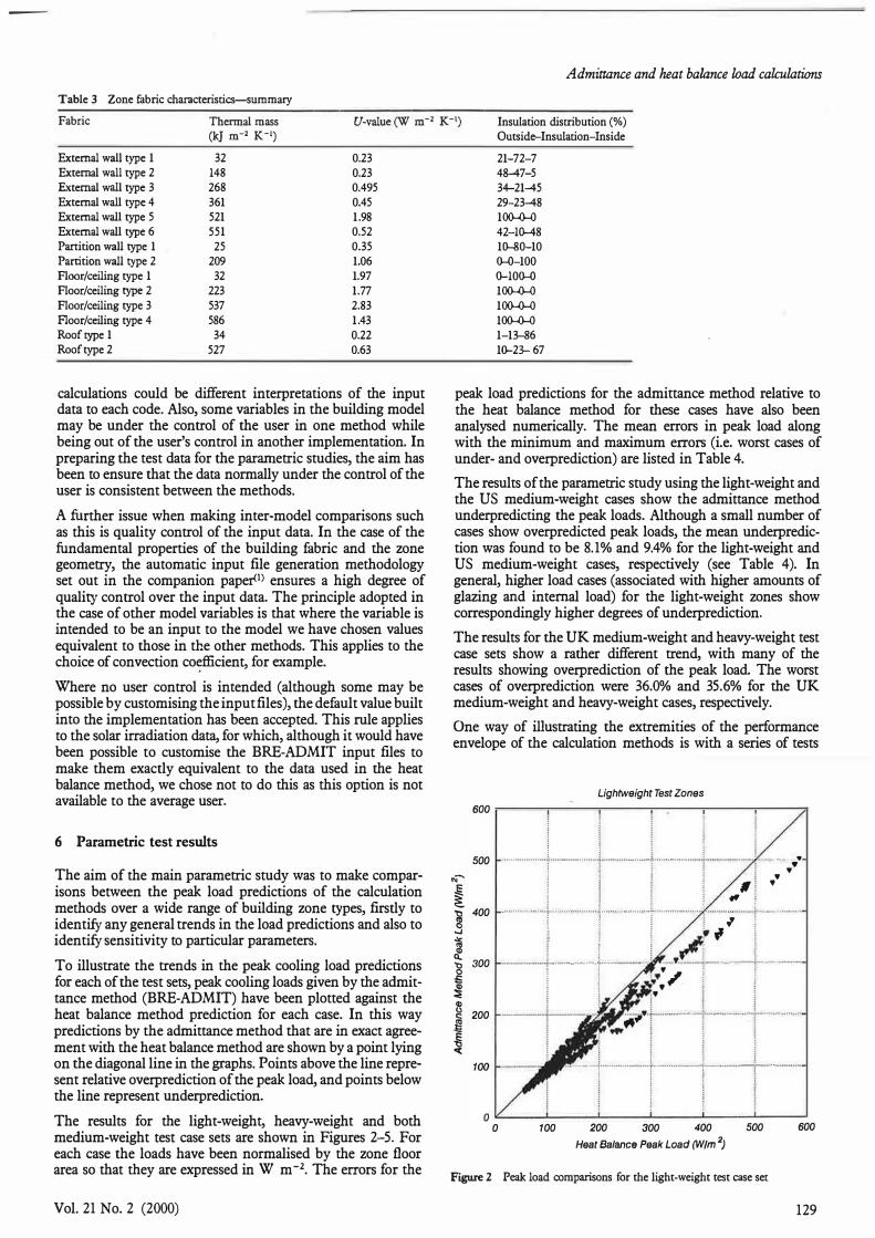
To illustrate the trends in the peak cooling load predictions for each of the test sets, peak cooling loads given by the admit­tance method (BRE-ADMIT) have been plotted against the heat balance method prediction for each case. In this way predictions by the admittance method that are in exact agree­ment with the heat balance method are shown by a point lying on the diagonal line in the graphs. Points above the line repre­sent relative overprediction of the peak load, and points below the line represent underprediction.

The results for the light-weight, heavy-weight and both medium-weight test case sets are shown in Figures 2-5. For each case the loads have been normalised by the zone floor area so that they are expressed in W m-2• The errors for the

Vol. 21 No. 2 (2000)

Admittance and heat balance load calculations

Insulation distribution (%)

Outside-Insulation-Inside

21-72-7

48-47-5

34-21-45

29-23-48 100--0--0

42-10-48 10-80-10

0-0-100

0-100-0

100--0--0

100--0--0

100--0--0

1-13--86

10-23-- 67

peak load predictions for the admittance method relative to the heat balance method for these cases have also been analysed numerically. The mean errors in peak load along with the minimum and maximum errors (i.e. worst cases of under- and overprediction) are listed in Table 4.

The results of the parametric study using the light-weight and the US medium-weight cases show the admittance method underpredicting the peak loads. Although a small number of cases show overpredicted peak loads, the mean underpredic­tion was found to be 8.1% and 9.4% for the light-weight and US medium-weight cases, respectively (see Table 4). In general, higher load cases (associated with higher amounts of glazing and internal load) for the light-weight zones show correspondingly higher degrees of underprediction.

The results for the UK medium-weight and heavy-weight test case sets show a rather different trend, with many of the results showing overprediction of the peak load. The worst cases of overprediction were 36.0% and 35.6% for the UK medium-weight and heavy-weight cases, respectively.

One way of illustrating the extremities of the performance envelope of the calculation methods is with a series of tests

.,. ....... � � 'tl l!l ...J

... i '8 £ � Q) () c: � .g "(

600

500

400

300

200

Ughtweight Test Zones

I !

··-··-··· .. ··· .. ·t·····-···-······ .. 1-··-·-···-··�·

t······-.···· .. ······f-

···········-········l ··�···

;

···�··

i J ' ; If' " ! j � .,, � � J • I -...... _ ......... r-..... ........ ..... 1 .................... T .......... -....... � ......... � .. ·-·-

r

· .. -........... . � l ! ,;l � l

�-.................. L ....... _.� .. ...... 1 .... -..... .-.. .... t -·-•r:. ... 1 ..... --....... --.lu . ....... __ _ I ' " ' ' i j .., • .,, ; i I 1 �" ;

-" ----1 --- ! ..... �f- ---1 --- +-- - -

i ---t- -1---1--i -·

0 "--��.._��-'--��-L��---L���'--�---' 0 100 200 300 400 500 600

Heat Balance Peak Load (W/m 2)

Figure 2 Peak load comparisons for the light-weight test case set

129

SJ Rees et al.

600

500

"E' � al 400

.9 ""' "' ID a.. '8 300

� � ID 0 200 c: "' E E "O < 100

0 0

US Mediumweight Test Zones

i ···t··········· ··"······1···-·······-l' .......... ........ r- ·-·-............. , .... ......... � ... ..

I 1 i 1 ,.;r - - ···--...... ., .... i ........ _.-l ..................... ! ....... ............. 1-.,. .. ---� .. .. 1 ................... .

f i � t • �

- -

·! --+- -:��r-+-- -I i •;. l .............. .... � .. ------ 1 " ........ ,, .. � .................... J ...................... } ................... . : r" ! I ' i !W l I f I ! !

'""""••-·i--•-••----••••·�••tll"·''""''"n••••••!.•••••••••••••''''''"b '''''-•.,..•-·•-••

100

� l i f I I • : I i I l ; ; I ;

200 300 400 500

Heat Balance Peak load CN/m2

)

600

Figure 3 Peak load comparisons for the US medium-weight test case set

Heavyweight Test Zones

500

"E' � "O 400 "' .9 -"' "' ID a.. "O 300 0 � � Q) 0 c: 200 "' E E "O <

Heat Balance Peak Load CN/m2

)

Figure 5 Peak load comparisons for the heavy-weight test case set

using only the maximum and minimum values of the para­meters. This has been done for a test series with 2048 cases and the results are plotted in Figure 6. Some of the loads can be seen to be very high. This arises from using the extreme parameter values. For example, some zones may have a very large glazing area in relation to the floor size owing to high aspect ratio, in addition to a large internal load.

In Figure 6 certain clusters of results can be seen for cases with higher loads. These represent cases with similar parameter combinations. In particular, a number of clusters of results show slight overprediction, while several others show large degrees of underprediction of the peak load. By sorting the results it was possible to identify the former cases as those with light-weight floors (floor type 1) and the latter cases as

130

! i I I

UK Mediumweight Test Zones

r ! . I 500 .... .. ----·1 .. -·----.. ··· '"I "''-""'""'"'·

r

--·--··· .. ··· .. -1 .. ....... .......... i ···- ............ .

� .ac - - --�- -t--_j, _ _ £ / _ __ __ j __ � ' i � 1 I

I� ---- t - -- lei-i---l-- - 1 - -,-� 1 l: .. ;z. i i ! < 1 ""' i ! i : ; ; l

:--··---·····r·--·�-··········1····-···--·r·-·····--··-

� r ! ; : :

: i � t ................... l ........... . ......... T ......... � ...... 1 .. ...... -.......... T ............ _

! i I I 0 "----'----'-----'----L----'------'

0 100 200 300 400 500 600 Heat Balance Peak Load (W/m 2)

Figure 4 Peak load comparisons for the UK medium-weight test case set.

'"e � "O "' .9 -"' "' ID a.. "O 0 � Oi � Q) 0 c: «I E E "O <

Minimum-Maximum Parameter Combinations

2500 �---�---�---�---�---�

2000

1500

1000

500

Floor 1 Floor4

.. • �

I l i I ! 1 i ............. _ . .... l . . ....... .......... ..... l"' ........................ , ......... _ ...... ........ ;··· .................. ..

I : I j I i # # I ' I I

............... _.,_.+.,_ ...... .... _,,, .... . j._............... : . ............ ,,r..,r..j .... ,_ .... , ....... .. . ; ; I -- I f , , i T...... ! ; ' I ! ! � N l ....... ' .......... , ,_ .. 1.. . ... ... .. .. . .. . .. . . .... . .......................... .i ........................... l ........... ··-.. _ ...... '. l �, I . 1 j fl/I' 1 ! : __,,, ... ,.,,.,,J.,,,., .. ,,,.,,,,. ... , ... , .. ! .... , , _ _., ... ,,_ . .,.,.,,l, ........ u ... ,1'''' .. r"

1 ! l ; ; I

I i I 0 =------'---___ _.._ ___ _.._ _ __ _._ _ __ �

0 500 1000 1500 2000

Heat Balance Peak Load CN/m2)

2500

Figure 6 Peak load comparisons for the minimum-maximum parameter

combination test cases. Results for zones with light-weight floors (floor 1) are

shown separately from those with heavy-weight floors (floor 4)

those with heavy-weight floors (floor type 4). The cases with different floor types have accordingly been identified sepa­rately in Figure 6. As the cases with high loads such as these all have 90% glazing, it is chiefly the floor construction that determines the thermal mass of the zone. Thus the same trend is shown: heavy-weight cases are overpredicted and light­weight cases are underpredicted by the admittance method compared to the heat balance method.

In addition to the peak hourly load, the time of occurrence of the peak is also of interest. The difference in the predicted hour of the peak load has been analysed for the 2048 cases with minimum-ma.xi.mum parameter combinations. Table 5

Building Services Engineering Research and Technology

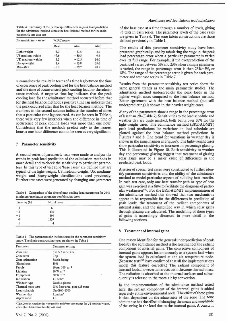
Table 4 Summary of the percentage differences in peak load prediction for the admittance method versus the heat balance method for the main parametric test case sets

Parametric test case set % Difference

Mean Min. Max.

Light-weight -8.0 - 31.5 8.l US medium-weight -7.6 - 30.5 9.4 UK medium-weight 3.5 - 1 2.5 36.0 Heavy-weight l .4 - 13.8 35.6 Min-Max -5.0 - 39.7 28.8

summarises the results in terms of a time lag between the time of occurrence of peak cooling load for the heat balance method and the time of occurrence of peak cooling load for the admit­tance method. A negative time lag indicates that the peak cooling load for the admittance method occurred before that for che heat balance mechod; a positive time lag indicates that che peak occurred after that for the heat balance method. The numbers in the second column indicate the number of times that a particular time lag occurred. As can be seen in Table 4, there were very few instances when the difference in time of occurrence of peak cooling loads was more than one hour. Considering that the methods predict only to the nearest hour, a one hour difference cannot be seen as very significant.

7 Parameter sensitivity

A second series of parametric tests were made to analyse the trends in peak load prediction of the calculation methods in more detail and to check the sensitivity to particular parame­ters. In this type of test zone 'base cases' are defined that are typical of the light-weight, US medium-weight, UK medium­weight and heavy-weight classifications used previously. Further test cases were generated by changing one parameter

Table 5 Comparison of the time of peak cooling load occurrence for 2048 minimum-maximum parameter combination cases

Time lag (h) No. of cases

-3 6 -2 130 - 1 599

0 1309 4

Table 6 The parameters for the base cases in the parameter sensitivity study. The fabric construction types are shown in Table 1

Parameter

Zone size Zone level Zone orientation Glazed area People Lighting Equipment Infiltration Window type Thermal mass type Load schedule Weather day Aspect ratio

Parameter setting

6 m X 6 m X 3 m Top South-facing 10% 10 per 100 m-2 20 W m-2 30 Wm-2 l.O ac h-1 Double-glazed 25% floor area, pine (25 mm) On 0800--1700 London* l.O

*The London weather day was used for each base case except for US medium-weight,

where the Phoenix weather day was used.

Vol. 21 No. 2 (2000)

Admittance and heat balance wad calculat.Wns

of the base case at a time through a number of levels, giving 95 tests in each series. The parameter levels of the base cases are given in Table 6. The zone fabric constructions are those defined previously in Table 1 .

The results of this parameter sensitivity study have been presented graphically, and by tabulating the range in che peak load percentage error when a particular parameter is varied over its full range. For example, if che overprediction of the peak load varies between 5% and 23% when a single parameter is varied, the range in percentage error is then 23%-5%, or 18%. The range of the percentage error is given for each para­meter and test case series in Table 7.

Results from the parameter sensitivity test series show the same general trends as the main paramerric studies. The admittance method underpredicts the peak loads in the lighter weight cases compared to the heat balance method. Better agreement with the heat balance method (but still underpredicting) is shown in the heavier weight cases.

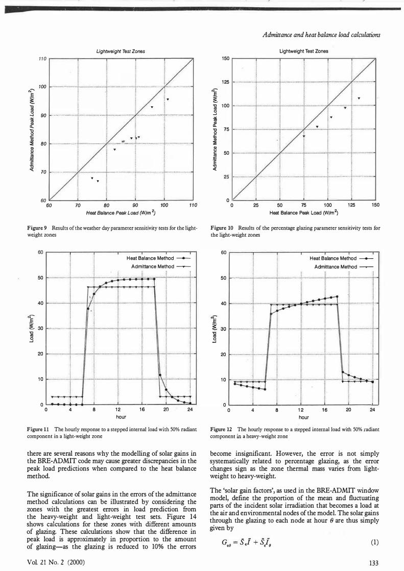
Many of the parameters show a range in the percentage error ofless than 2% (Table 7). Sensitivities to the load schedule and weather day are quite marked, both being over 10% for che light-weight cases. The admittance method (BRE-ADMIT) peak load predictions for variations in load schedule are plotted against the heat balance method predictions in Figures 7 and 8. The trend for variations in weather day is shown in d1e same manner in Figure 9. The light-weight cases show particular sensitivity to increases in percentage glazing. This is illustrated in Figure 10. Both sensitivity to weather day and percentage glazing suggest that n·eatmenc of glazing solar gains may be a major cause of differences in the predicted peak loads.

A series of special test cases were constructed to furcher iden­tify parameter sensitivities and che ability of the adminance mechod to model particular aspects of building hear transfer. In each test case, only one heat transfer path or type of heat gain was exercised at a time co facilitate the diagnosis of partic­ular weaknesses<18>. For the BRE-ADMIT implementation of the admittance method this showed that two mechanisms appear to be responsible for the differences in prediction of peak loads: the treatment of the radiant components

. of

internal gains, and the simplified way in which solar gains through glazing are calculated. The modelling of these types of gains is accordingly discussed in more derail in che following sections.

8 Treatment of internal gains

One reason identified for the general underprediction of peak loads by the admittance mechod is the treatment of the radiant component of internal gains. The convective component of internal gains appears instantaneously as a system load when the system load is calculated at che air te�perature n?de. (Separate tests<18l have confirmed chat all the unplemenrat1ons

_ model chis feature correctly.) The radiant component ot internal loads, however, interacts wich che zone thermal mass. The radiation is absorbed at che internal surfaces and subse­quently is released to the room air by convection.

In che implementations of the admittance mechod tested here, the radiant component of the internal gains is ad�ed separately at che environmental node. The effect of these gains is chen dependent on the admittance of the zone. The

.zone

admittance has the effect of changing che mean and amplnude of the swing in the load due to the internal gains. A constant

131

--- - - -

SJ Rees et al.

Table 7 The percentage error range for each parameter and each test series

Parameter Percentage error range

Light-weight US medium-weight UK medium-weight Heavy-weight

Zone size l.30 2.25

Aspect ratio 0.71 0.75

Zone orientation 3.19 4.04

% Glazing 6.46 1.68

Persons 0.24 1.25

Lighting load 0.89 3.27

Equipment load 3.76 1 .04

Infiltration 1.20 3.35 External wall type 1.69 1.23 Internal wall type 0.72 0.72 Roof type 0.25 0.25 Floor type 5.11 2.63 Window type 2.70 0.94 Thermal mass 1.44 1.25 Load schedule 10.98 6.88 Weacher day 10.11 7.81

Lightweight Test Zones

80

!

i j 1 75 ·-····················-···-r················ .............. r·--··· ·····-. . . . . . .......... ···-

···---···· ......... .

� ! I

3.56

5.12

2.42

0.82

0.64

0.72

1.91

1.13

2.06

0.72

0.25

3.88

3.73

4.54

6.34

8.6

� I I cf. 70 ,. ... . . ............ . ..... . . -..!. . .... -....... . . ... ... .. ..... . . �-'-··------·-- · ···· ···-·· ····�-- ............. .... ..... ...... .. -g i � ; � :

'� .,. � 1 - � � , T B j � C I I � ! i E ··········----�·· ............ J �-············· ·······--·--··L .................................... ! .... ...... . �-····· -·-······-·· "O 65 j : -< I !

!

60IL..����..l--����...l-.����--'-����-' 60 65 70 75

Heat Balance Peak Load CN/m2

)

80

Figure 7 Results of the load schedule parameter sensitivity tests for the light-weight zones

phase shift is introduced between the gain and the resulting load depending on the lag associated with the average zone admittance.

The effect of this approach is illustrated in Figures 1 1 and 12, which show the hourly response to an internal heat gain with 50% radiant component in typical light-weight and heavy­weight zones, respectively (all other gains have been elimi­nated in these cases). These results show the simplified nature of the interaction between the radiant heat gain and the zone thermal mass modelled by the admittance method. The result is an underprediction of the peak load for both light-weight and heavy-weight cases.

The response to internal gains predicted by the admittance method could be expected to be more realistic if the load schedule were sinusoidal rather than stepped, as assumed in the derivation of the fabric admittances. This has been demonstrated by applying a sinusoidal load schedule with a period of 24 h and peak of 50 W m-2 to a heavy-weight zone,

2.05

0.81

l.35

0.25

0.66

1.47

2.74

0.87

1.41

0.72

0.25

2.63

4.94

0.94

7.49

9.37

70 Heavyweight Test Zones

i : ! I i ' . · ·

-·····

· ..........

...

.. �

...... r- ··

·-··· .. -· ... -········- ···r · .....

........

-........ ..... ... � �···

--··· -.... ... ...

� . . .....

.

I i ll 1,: l .. � i "' I r " ! � 60 ··-···· · ···· · ···· · ····-- ·······1 ......... -....... -............ 1· .................... . ...

.......... J ....... -....... .... . ......... . � i t .. I

� i ! i c i i . "' i i i 55 ··-·-----···· ·····-······ ;-· · · .. --·- ···· ···· · - · - ··t·· · - · ······--················ ····1-- -·--··-.... .... ..

i ! 1 � T f � � � !

50!£......����"'-����-'-����...I....����-' 50 55 60 65 70

Heat Balance Peak Load CN/m2)

Figure 8 Results of the load schedule parameter sensitivity tests for the heavy-weight zones

rhe response to which is shown in Figure 13. There is closer agreement with the heat balance method results in this case, although the phase is approximately one hour different. This demonstrates one of the shoncomings of the assumption of sinusoidally varying gains made by the admittance method. Unfortunately, in the case of internal gains, where schedules are normally much closer to a stepped pattern, this assump­tion is not a conservative one.

9 Prediction of glazing solar gains

9.1 The sola.r gain factor wiruluw model

The sky models of rhe heat balance method implementation give slightly higher incident solar irradiances than that of the BRE-ADMIT code-see Appendix A of Rees et al <2). This may account for approximately 2% .of rhe difference between the results for the particular weather days used. However,

Building Services Engineering Research and Technology

Lightweight Test Zones

1 1 0 ,----..----""T"""-----r------.-----,,

� ! i 100 ..... --............. t ...... . .................. J ........ ..... � ... . ...... t ...... _ . .......... . . . . . . . i .. : . ... ....... .......... .

i ! � � l f l ; ., l ! i .. .

90 . . . ........ � ...... __ .i ........... _ ..... i . ..... . l .... ........................ i ... .. ,_ .. ,_ .......... �··i�· · · ··· .. ··· · ····· ···· .. . i I ; l I i ! 1 ... ;,... .

80 ............ ---·- -·1·-·-"''""-""''' ......... -.:1'!.-...... � .................. ........ 4 ..... _ ............... . . 1 i I -I i ' ' 70 ..... 1 -. - oH�O • O .. �O O-OO� OOOH< • t to n - • 00000t00•000 0 .. 0 0 0 0 .. 000 > 00000 0>l-······ ··· .. +•o•O•o•O••··�-······-·-···-·--·

I .. .. I l I ! i I t � i 60 �---....__-�-�---�---�---�

60 70 80 90 100 110 Heat Balance Peak Load (W/m 2)

Figure 9 Results of the weather day paramerer sensitivity tests for the light­weight zones

60 ,----..----..-----r----..------.----.--i Heat Bal ance Method -+--

Admittance Method --..---i : ! t I

50

40

. , 1 i � 30 ..... . ,._ .. ,_

: �-: �I� -�--���=r-.� -r��___r ; : : t t � ! !

0 L-..1�-+-+--+-+--'------'----'-----'---=:l"--' 0 4 8 12

hour

16 20 24

Figure 11 The hourly response to a stepped internal load with 50% radiant component in a light-weight zone

there are several reasons why the modelling of solar gains in the BRE-ADMIT code may cause greater discrepancies in the peak load predictions when compared to the heat balance method.

The significance of solar gains in the errors of the admittance method calculations can be illustrated by considering the zones with the greatest errors in load prediction from the heavy-weight and light-weight test sets. Figure 14 shows calculations for these zones with different amounts of glazing. These calculations show that the difference in peak load is approximately in proportion to the amount of glazing-as the glazing is reduced to 10% the errors

Vol. 21 No. 2 (2000)

Admittance and heat balance load calculations

Lightweight Test Zones

150

125

NE [ 'tl 1 00 "' 0 -' -a "' Cl.. 'tl 75 0 � ::? 8

50 1ij E E 'tl < I I ! j l 25

l I : 1 I -···"·---·; ...... _ .... _ .. ....

. !.. ..... _.,, . ....... +· · ••"""""""-+---.. -··-.. · · ·?··· .. · · · .. -·-·""

! 1 i I i i : l : i ! I I � ! : t I : I 0

0 25 50 75 1 00 125 1 50

Heat Bal ance Peak load CN/m2)

Figure 10 Results of the percentage glazing parameter sensitivity tests for

the light-weight zones

60 �--�---.----�---.-----r----.--. Heat Balance Method -+--

i Admittance Method -T---

50 i i - r . . - -- - .-- - -r - - !- - - --r--- -r--1

40

20

10

: : : F"""'9;:o;l'""'��'l""' ... F ... "'. ·""- -,,- ··········r··· .. ···· .... · ········r·

I I

. .. .. :.

0 '-----'-----'------'----'-----'----..........

0 4 8 12

hour

1 6 20 24

Figure 12 The hourly response to a stepped internal load with 50% radiant

component in a heavy-weight zone

become insignificant. However, the error is not simply systematically related to percentage glazing, as the error changes sign as the zone thermal mass varies from light­weight to heavy-weight.

The 'solar gain factors', as used in the BRE-ADMIT window model, define the proportion of the mean and fluctuating parts of the incident solar irradiation that becomes a load at the air and environmental nodes of the model. The solar gains through the glazing to each node at hour 8 are thus simply given by

(1)

133

SJ Rees et al.

1 � 30

0 '--��...._��-'-��__._��---"���'--��-'-' 0 4 B 12

hour

1 6 20 24

Figure 13 The hourly response to a sinusoidal internal load with 50%

radiant component in a heavy-weight zone

and

G.8 == S .J + S/8 (2)

where Sc and s. are che mean and alcemating solar gaiy. factors for che environmencal point, and similarly S. and S are for rhe air poinc. The principal gains are at the enviro:imental node. Gains ac the air· node are due to convection from internal blinds, etc., adja_cenr the inside surface of the window.

Solar gain factors are tabulated in che 1986 CIBSE Gui.d/.8> (Tables A8.2 and A8.6) for souchwest-facing light-weight and heavy-weight rooms in a London location and for various window/shade combinations. This method of calculating che load due co u·ansmission and absorption of solar radiation through the glazing makes a number of simplifications and assumptions:

134

The proportion of solar irradiation that becomes a load in the room is assumed to be fixed, and so no account is taken of the effect of different angles of incidence of the solar beam cicher at each hour of the day or at different latitudes. (The latter problem could be addressed by CIBSE publishing solar gain factor data for a range oflati­cudes other than London.)

The response of a building zone to transmitted and absorbed solar irradiation depends heavily on its thermal mass. Relying on only two sets of factors derived for a typical light-weight and a typical heavy-weight zone means that zones of different construction cannot be represented adequately.

The solar gain factors in the 1986 CIBSE Gui.de<8> have been calculated for southwest-facing windows. At the peak hour the factors define the. proportions of the mean and fluctuating pans of the solar gains. The incident solar irradiation on south-facing surfaces differs somewhat from that on east- and west-facing surfaces when m·eraged over 24 h. The same factors applied to windows exposed to solar irradiation from other directions will not there­fore reproduce the correct peak load.

250

"'e 200 �

lightweight zone • 1

Heavyweight zone • . .......... r .. -.... ····----·r--.. ····-·· .. ····: ..... .

·,.1 I • ! I . . l • ! . � ....................... i ............. �-.... -···f·· ···--·····-····1······· ... ···············1 ············-·-·····-r·-··· i i i I ! ! ! � j t l ! • I .. I . I 150

- -- - r - - r:-- - :1 � - � � r -··----- -

--T

i 100 -- - :.i -- -;-; ·:l: - :-�- - 1--- --- 1-- --�,; ..... . ·e ' • . ' I , � 50 -···--········-·······1 ·-··-············-L ................... .J... ..................... . L .. ___ ........... : . .... .

I I ! I I t I • !

0 .._ __ __._ ___ ....._ __ ___. ___ __._ ___ ..____.

0 50 100 150 200 Heat Balance Peak Load �/m2)

250

Figure 14 The effecc of varying cbe percentage of glazing on che light-wcighl and heavy-weight :rones with the worst-case errors. The percentage gla?lng varies from 10% co 90% ip 10% steps

In view of these simplifications and assumptions it could be expected that considerable improvement in performance could be gained by use of a more detailed window model in the admittance method calculation. Subsequently to the orig­inal parametric studies discussed above, the authors have implemented a second admittance-method code that has a detailed window model but otherwise is similar to the BRE­AD MIT implementation.

9.2 The detailed window model

This model is based upon an analysis presented by Jones<18), where it is assumed that the glass is homogeneous so that Snell's law can used to determine the angle of refraction from knowledge of the refractive index of the glass (1 .52 for clear glass). Thus, given the angle of incidence, the reflectivity of the glass can be calculated. A second, fundamental property of the glass is the extinction coefficient (about 0.033 mm-1), which enables calculation of the absorbed radiation. The model treats direct and diffuse radiation separately, the trans­mission and absorption of diffuse radiation being the average for all angles of incidence. It is recognised that not all glasses can be represented by this simple theory, so either the extinc­tion coefficient is calculated using manufacturer's data or published data can be curve-fitted to provide the necessary information.

The thermal exchange between the glazing and the zone comprises three elements:

direct transmission

radiation from the surface of the glazing

convection from the surface of the glazing.

In the case of single glazing, the direct transmission is deter­mined from the theory outlined above. A heat balance of the glazing will enable calculation of the glass cemperamre and thus the convective and radiative exchanges are obtained. Where multiple panes are involved, it becomes necessary to take account of the numerous reflections that occur between

Building Services Engineering Research and Technology

panes. Thus the transmission coefficient for a double glazed window becomes

(3)

where T is the transmission coefficient, p is the reflection coef­ficient and the subscript o is for the outer pane and i for the inner pane.

Similarly the radiation absorbed at the inner and outer panes is

(4)

where A is the absorption coefficient. The absorption coeffi­cienr may be obtained similarly for the inner pane.

The glazing temperature is then calculated from an energy balance on the complete glazing system. The absorbed radia­tion in each pane is equated to the convection and radiation from each pane, which results in the development of a pair of simultaneous equations that are solved to yield the tempera­ture of the glazing. The solar component of the cooling load is calculated on the assumption that internal and external temperatures are identical. The transmission gain is deter­mined as a separate component.

The implementation of the admittance method with the detailed window model has been tested against the heat balance method using the same light-weight and heavy­weight parametric test series as the BRE-ADMIT implemen­tation. Analysis of these results showed a distinct correlation between the differences in peak load prediction and the type

"'E' 450 � 400 al 350 .3

250 200

t.:lt:l:f :E�jt: ; : : : : I l ; 0 "---'---'--'--......___,__. _ _.____.___.__.

� 450 � 400 ""C <II 350 .3 � 300 ., 0..

I 250 200 ==

., 150 0 c: � 100 E � 50

0

Admittance and heat balance load calculations

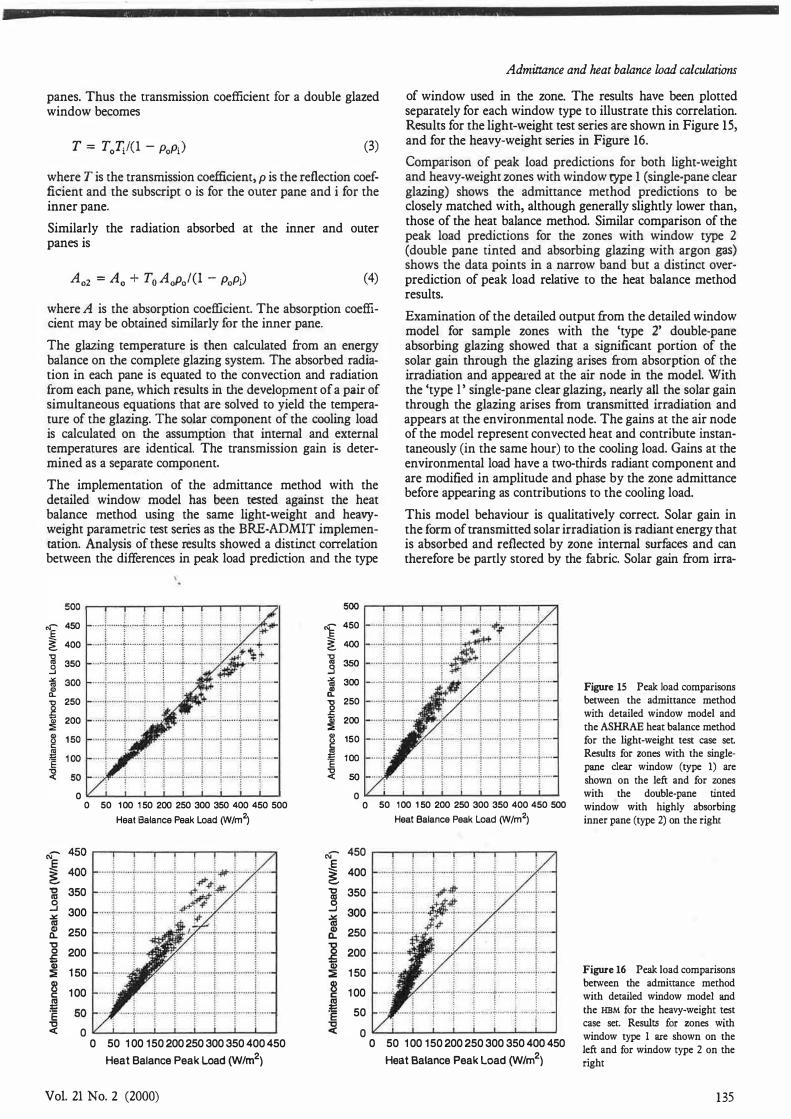
of window used in the zone. The results have been plotted separately for each window type to illustrate this correlation. Results for the light-weight test series are shown in Figure 15, and for the heavy-weight series in Figure 16.

Comparison of peak load predictions for both light-weight and heavy-weight zones with window type 1 (single-pane clear glazing) shows the admittance method predictions to be closely matched with, although generally slightly lower than, those of the heat balance method. Similar comparison of the peak load predictions for the zones with window type 2 (double pane tinted and absorbing glazing with argon gas) shows the data points in a narrow band but a distinct over­prediction of peak load relative to the heat balance method results.

Examination of the detailed output from the detailed window model for sample zones with the 'type 2' double-pane absorbing glazing showed that a significant portion of the solar gain through the glazing arises from absorption of the irradiation and appeared at the air node in the model. With the 'type l ' single-pane clear glazing, nearly all the solar gain through the glazing arises from cransmitted irradiation and appears at the environmental node. The gains at the air node of the model represent convected heat and contribute instan­taneously (in the same hour) to the cooling load. Gains at the environmental load have a two-thirds radiant component and are modified in amplitude and phase by the zone admittance before appearing as contributions to the cooling load.

This model behaviour is qualitatively correct. Solar gain in the form of transmitted solar irradiation is radiant energy that is absorbed and reflected by zone internal surfaces and can therefore be partly stored by the fabric. Solar gain from irra-

0 50 100 1 50 200 250 300 350 400 450 500 Heat Balance Peak Load rN/m

2)

0 50 100 1 50 200 250 300 350 400 450 500 Heat Balance Peak Load rN/m2)

Figure 15 Peak load comparisons

between the admittance method

with detailed window model and

the ASHRAE heat balance method

for the light-weight test case set.

Results for zones with the single­

pane clear window (type 1) are

shown on the left and for zones

with the double·pane tinted

window with highly absorbing

inner pane (type 2) on the right

N' 450 �-�-......-��.---�-......-....,.

al 350 .9 300 � 250 'C 0 200 i � 1 50

j 1 00 E � 0 "---�--'--'---'----'�.....__.__..._____, 0 50 1 00 150 200 250 300 350 400 450

Heat Balance Peak Load (W/m2)

Vol. 21 No. 2 (2000)

,E 400 � 'C 350 .9

250 200 1 50 1 00 t - . � 1 � � �

.

· · · · · · ·r·-····1·······1- · · · · ·r·:· · · · ·;u······r····

50 .... · · ···· 1· · · · · · ··1········ 1 ···· .... 1 · · · · · · ·1· · - · · · ·i-·······1· · · · · ·

� ! : ; � 0 ,.___�____,__..._����____,_�..._� 0 50 1 00 150 200 250 300 350 400 450 Heat Balance Peak Load (W/m2)

Figure 16 Peak load comparisons

between the admittance method

with detailed window model and

the HBM for the heavy-weight test

case set Results for zones with

window type 1 are shown on the

left and for window type 2 on the

right

135

SJ Rees et al.

diation absorbed at the inner pane of the glazing results in convection of heat from the inner surface, and therefore contributes instantaneously to the cooling load. (This is strictly true only for 'all air' cooling systems. In this work only cooling by the air stream is considered.).

Although we have no reason to suspect that the total solar energy (transmitted and absorbed) predicted by the detailed window model is very different from that predicted by the window model in the heat balance method, different peak load predictions could be expected depending on how th� ener� is divided between transmitted and absorbed components. To examine this it is necessary to consider the basis of the window model used in the heat balance method.

9.3 The solar heat gain coefficient window nwdel

The window model currently implemented in the heat balance method is based on the concept of solar heat gain coef­ficient (SHGC). The total heat gain per unit area, qi, flowing into a zone through multiple-pane glazing can be expressed as

(5)

where E. is the total solar irradiance (diffuse, ground reflected and dir�ct), T is the overall solar transmirtance, A c is the effective front �olar absorptance of the jth layer in the

1 system

and (N1) is the inward flowing proportion of the absorbed radiatioii of the jth layer. The solar heat gain coefficient is defined as the fraction of the incident irradiation that becomes inwardly flowing heat gain, so that equation 5 can be written (ASHRAE Fundamentals Handbook 1997, Chapter 29, Eq.24)

q. = E. · SHGC 1 1 (6)

According to the (US) National Fenestration Rating Counci1C21l, the preferred way of calculating the SHGC is to inte­grate over the solar spectrum using the glazing spectrally dependent properties. In addition, the SHGC is strictly depen­dent on the angle of incidence. This suggests the use of an angularly dependent SHGC to calculate the solar gains due to direct irradiation, and a value integrated over a hemisphere to deal with gains due to diffuse irradiation. However, it . is often only the SHGC at normal incidence that is available from glazing manufacturers.

In the window model implemented in the heat balance method, the normal SHGC is used to determine the properties of the window. So that the angular dependence of the SHGC can be accommodated, the normal value is modified by the angularly dependent transmittance for a single pane of stan­dard clear glass, r j {}), normalised by dividing by the normal transmittance, T..i�· The solar gain due to direct irradiation is then modelled as

(7)

where E0 is the direct irradiance and SHGCn is the normal solar heat gain coefficient. There is an assumption here that the transmittance and absorptance of the glazing being modelled vary with incidence angle in the same way as those for stan­dard clear glazing. This is not necessarily true for more advanced multipane glazing systems.

The sky diffuse and ground-reflected solar irradiation are treated separately from direct irradiation in the heat balance method window model. In this case the assumption is made

136

that the transmittance at 60° incidence angle is representative of the value integrated over a hemisphere, so that

(8)

where Editr is the total diffuse irradiance, and qwtr is the associ­ated gain per unit area of glazing.

The way in which the solar gains (q0 and qwtr multiplied by the appropriate areas) appear in the zone model is of great signifi­cance in determining the response of the zone. In the heat balance method all of the solar gains are treated as radiation. The direct solar gains appear as terms in the surface heat balance for the floor and the diffuse solar gains from the glazing appear as terms in each surface heat balance, after being distributed on an area-weighted basis.

It becomes necessary to ignore the convection arising from the absorbed solar gains in this way owing to the nature of the solar heat gain coefficient. When the absorbed and transmitted energy components (the terms of equation 5 in square brack· ets) are combined in the calculation of the solar heat gain coef­ficient, all the information about the split between transmitted and absorbed energy is lost. In a model relying on the SHGC it therefore becomes necessary to make an assumption about the division of the solar gain between absorbed and transmitted components. Treating all the gains as radiation within the zone model is reasonable only for windows with low absorp· tance (i.e. with similar properties to those of clear glass).

The lack of explicit calculation of the absorbed component of the glazing solar gain in the heat balance method may there­fore be the reason for the differences in calculation of peak load when compared to the admittance method with the detailed window model for zones with the absorbing glazing. To test this hypothesis further, an implementation of the admittance method with the same solar heat gain coefficient window model as in the heat balance method was developed. The results of the calculations of the peak load with this code for the heavy-weight test cases are shown in Figure 17. In this case the results for zones with either window type show good agreement.

One further way to test the different effects of the treatment of the solar gains in the zone is to artificially convert some of the solar gains to convective gains. This is possible by including an internal blind in the zone description used by the heat balance method. Blinds were included with zero transmittance so that all the solar gains arriving at the internal blind became convection rather than radiant energy. This does not ensure quantitatively correct results but serves to illustrate the effect of making the opposite assumption about the treatment of the glazing solar gains in the zone model. The results for the heavy-weight zones with the absorbing glazing are shown in Figure 18. The peak loads predicted by the heat balance method have accordingly increased for each test case so that there is better agreement with the results of the admit· tance method calculations with the detailed window model.

10 Conclusions

Design-day cooling load calculations have been made using the ASHRAE heat balance method and the BRE-ADMIT imple· mentation of the CIBSE admittance method for more than 7000 different combinations of zone construction, orientation, internal loading and weather day. Additional calculations have been made to study the effects of different window modelling

Building Services Engineering Research and Technology

Admittance and heat balance load calculations

� 450 ,--...,---,.-..---r-----,..---.---,.-.,...-...,. 1 400 -g 350 .9 300 � Q) D.. "8 � ::E

250 200 150

.. j·····t + ···t i·��;;!�l : ·

: : : : : : t :

+1 L��rr r •OOOOl-...••.• ;. ...� .••• : ...... U.1000000.lOOO•O <Oi ..... HO�OOO•OO

E l l � � � l ...... �... ·····-�····· .. -� ..... ... } .. . : .. +.·-···f·······-l-·-···

::::r:::::r:::::r:::::r:::::r::::r::::r:�:::,i:: :::· . . .... ; ..... �-� . . .. .... i . .. . .. . . i ..... . . J __ ____ ; ...... J . ..... . . t. . .•.

"O 350 �

� 1 00 J ! : i;�trt t l

··---·f··· : ·····-�---· ···i· ··· ·- ·1····· ··1·······-��·-· .. ··t······

250 200 1 50

: ! ; ! : : � : 50 ; : � : ; ! : ; -·�· � -·· .. -

r·-- · - -T·--� -·

T·� .. ··r

······r�··-·-r

· .. ·-··1· ·---- �

E �

50 .. .. ' ...... l ........ l� ...... L.. . .. . L ..... i ........ ( ........ j ..... . : : : : i ; !

Figure 17 Peak load comparisons between the admittance method with the SHGC window model and the HBM for the heavy-weight test case set. Results for zones with window type 1 are shown on the left and for window type 2 on the right

2 ; : ; : : : 0 ..___.___._...__.__...___.__.._..____, 0 .____.__..��_.___.....__...__..._�_, 0 50 1 00 1 50 200 250 300 350 400 450 0 50 1 00 150 200 250 300 350 400 450

N-E �

"C ca 0 -I � ca Q) a.. "C 0 ..c: -Q) :2 Q) C.) i:: ca = ·e "C <(

450

400

350

300

250

200

1 50

1 00

50

Heat Balance Peak Load (W/m2)

. . . . . . L . . . . . . . . . .... . . f . . ·- · · · ·! · - · - ·-· 1· - · · . . . . � -+·--f .!. . . --l-· - -·-

. . . . . . i . . . .. . . . . j . . .... . . . � . . . .. .. + .. . . . .. 1 . . ·:

·t ·1: . . . . . . + · · - . . . . . . i :f. . . ·--· ·r ··--. . r-·· ·T .. . . . "T .. . 4t*+ �,: . . . . . . . . r- - - - - - - - 1 ...... . . . . . . : . . . . . . . . � . . . . . . . . r . . . . -#; . . · - - - ·

r--· · · ·

(· · · · · - -

j· · · ···

. . . ' . . . . . ' . . · · · · · · : · · · · · · · · -:· · · ·· .. · · ·:-· ··· · · ·· : · ·· ·····:·········:··· · · · · ·: · · · · · · . j .t : . :

. ' . . . ··· · · •! • • ·· · · ·· ; · · · · ·· · · :· · · ····· ·:-·· · · · • ·! · · · ··· . : : : : : •••• •• ; ......... ; 0-••••••• ; • • • • • • • • • : • • • • • • • • • ;. • • • • •••• 1 . . . . . . . . . . . . . . . . . ' ; j . . . � . . . .. . > . . . . '1"" ' "'(" " ' " ' ]" " " "1"" " " " '[" " " "( ' " '

0 ..__..___..___..___...__.___..___..___.._____, 0 50 1 00 1 50 200 250 300 350 400 450

Heat Balance Peak Load (W/m2)

Figure 18 Peak load comparisons between the admittance method with detailed window model and the HBM for the heavy-weight test zones with window type 2. Here the blinds have zero transmittance in the HBM zone descriptions

practices. From the results of these parametric studies, the fol­lowing can be concluded.

The interaction between the zone fabric and internal gains in the admittance method is treated only simply. For internal gains with the usual 'step shaped' schedule, this was found to result in underprediction of the peak load for both light-weight and heavy-weight zones.

The BRE-ADMIT implementation of the admittance method was found to underpreclict peak load for light­weight cases and overpredict peak loads for heavy-weight cases when compared to the heat balance method. This is principally due to the use of the simplified 'solar gain factor' window model in this implementation of the admittance method.

The results of calculations with an implementation of the admittance method using a detail window model showed good agreement with the heat balance method for zones with single-pane clear glazing. The heat balance method always predicted comparatively lower peak loads for zones with a double-pane window with absorbing glass.

Vol. 21 No. 2 (2000)

Heat Balance Peak Load (W/m2)

The 'solar heat gain coefficient' window model used in the heat balance method treats all of the solar gains as radiant energy wl;ien calculating the zone heat balances. With windows that have highly absorbing glass, ignoring the convective component of the absorbed solar gains in this way results in underprediction of peak loads.

It has been shown how the results of the admittance method can be improved by the use of a more advanced window model. The solar gain factor window model was originally intended for use in manual calculations of summertime temperatures with the admittance method. The computing power available to most engineers has clearly increased considerably since the introduction of the admittance method and also since the publication of the BRE-ADMIT code. In any computer implementation of the admittance method, there can therefore be little reason not to use a more advanced giazing model, as has recently been done in the publication of the revised CIBSE Guide A : 1999<11l.

It could be said that the solar heat gain factor window model is not 'endemic' to the heat balance methods-a variety of window models are feasible in a heat balance approach. In some ways the simplified namre of this window model is contrary to the heat balance philosophy. It must be acknowl­edged that the solar heat gain factor model has the advantage that that such factors are commonly available for fenestration products. Detailed window models require much more detailed data about the properties of each pane, which are not always available. It would, however, be beneficial to users of the heat balance method to be able to use a more detailed window model where detailed property data are available.

Acknowledgements

This work was carried out under a joint ASHRAE and CIBSE fonded project 'Comparison of Load Calculation Procedures' (ASHRAE 942-RP, CIBSE 22/95). The authors also thank C. Wilkins (Hallam, Inc.), D. Arnold (Troup Bywaters & Anders) and Ove Arup & Partners for their help in providing details of building fabrics.

References

Spitler J D and Rees S J Quantitative comparison of North American and UK cooling load calculation procedures-Methodology ASHRAE Trans. 104(2) 36-46 (1998)

2 Rees S J, Spitler J D and Haves P Quantitative comparison of North American and UK cooling load calculation procedures-Results ASHRAE Trans. 104(2) 47-61 (1998)

137

SJ Rees et al.

3 Romine T B Cooling load calculation: art or science? ASHRAE J. 34(1) 14-24 (1992)

4 Pedersen C 0, Fisher D E and Liesen R J Development of a heat balance procedure for calculating cooling loads ASHRAE Trans. 103(2)

459-468 (1997)

5 Spitler J D Fisher D E and Pedersen C 0 The radiant time series cool­

ing load calculation procedureASHRAE Trans. 103(2) 503-515 (1997)

6 ASHRAE 1997 ASHRAE handbook-Fundamentals (Atlanta:

ASHRAE, Inc.) (1997)

7 McQuiston F C and Spitler J D Cooling and lwating load calculation manual 2nd edn (Atlanta: ASHRAE, Inc.) (1992)

8 CIBSE Guide A-Design Data (London: CIBSE) (1986)

9 Dancer E Periodic heat flow characteristics of simple walls and roof

]. Inst. Heating and Ventilating Engineers 28 136-146 (1960)

10 Loudon A G Summertime temperatures in buildings without air conditioning Building Research Station Current Paper 47/68 (also J. Heating and Ventilating Engineers 32 280-292, 1970) (1968)

11 GIESE Guide A-Design Data (London: CIBSE) (1999)

12 Dancer E Room response according to CIBSE Guide procedures

Building Sero. Eng. Res. Technol. 4(2) 46-51 (1983)

138

13 Bloomfield D P BRE-AD1'-IUT: Thmnal design of buildings (Watford: BRE Publishing) (undated)

14 Rees S J, Spitler J D, Davies M G and Haves P Qualitative comparison of North American and UK cooling load calculation methods Int. J Heating, Ventilating, Air-Conditioning and Refrigeration Research 6(1) 75-99

15 Walton G N A New algorithm for radiant interchange in room loads

calculations ASHRAE Trans. 86(2) 190-208 (1980)

16 BLAST Support Office ELA.ST (building loads and system tlwrmody­namics) (Urbana-Champaign: University of Illinois) (1980)

17 Walton G Thmnal analysis research program reference manual (Washington DC: National Bureau of Standards) (1983)

18 Rees S J and Spitler J D Proposals for a building load diagnostic test

procedure ASHRAE Trans. 105(2) 514-526 (1999)

19 Jones R H L Solar radiation through windows-theory and equations

Building Sero. Eng. Res. Technol. 1(2) 83-91 (1980)

20 NFRC Procedure for determining fenestration product solar heat gain

coefficients at normal incidence. Standard 200-95 (National Fenestration

Rating Council) (1995)

Building Services Engineering Research and Technology