Aalborg Universitet

Comparison of Model-Based Control Solutions for Severe Riser-Induced Slugs

Pedersen, Simon; Jahanshahi, Esmaiel; Yang, Zhenyu; Skogestad, Sigurd

Published in:Energies

DOI (link to publication from Publisher):10.3390/en10122014

Creative Commons LicenseCC BY 4.0

Publication date:2017

Document VersionPublisher's PDF, also known as Version of record

Link to publication from Aalborg University

Citation for published version (APA):Pedersen, S., Jahanshahi, E., Yang, Z., & Skogestad, S. (2017). Comparison of Model-Based Control Solutionsfor Severe Riser-Induced Slugs. Energies, 10(12), [2014]. DOI: 10.3390/en10122014

General rightsCopyright and moral rights for the publications made accessible in the public portal are retained by the authors and/or other copyright ownersand it is a condition of accessing publications that users recognise and abide by the legal requirements associated with these rights.

? Users may download and print one copy of any publication from the public portal for the purpose of private study or research. ? You may not further distribute the material or use it for any profit-making activity or commercial gain ? You may freely distribute the URL identifying the publication in the public portal ?

Take down policyIf you believe that this document breaches copyright please contact us at vbn@aub.aau.dk providing details, and we will remove access tothe work immediately and investigate your claim.

Downloaded from vbn.aau.dk on: maj 19, 2018

energies

Article

Comparison of Model-Based Control Solutions forSevere Riser-Induced Slugs

Simon Pedersen 1,* ID , Esmaeil Jahanshahi 2, Zhenyu Yang 1 and Sigurd Skogestad 2

1 Department of Energy Technology, Aalborg University, Esbjerg DK-6700, Denmark; yang@et.aau.dk2 Department of Chemical Engineering, Norwegian University of Science and Technology,

Trondheim NO-7491, Norway; esmaeil.jahanshahi@hotmail.com (E.J.); skoge@ntnu.no (S.S.)* Correspondence: spe@et.aau.dk; Tel.: +45-3066-3663

Received: 22 September 2017; Accepted: 23 November 2017; Published: 1 December 2017

Abstract: Control solutions for eliminating severe riser-induced slugs in offshore oil & gas pipelineinstallations are key topics in offshore Exploration and Production (E&P) processes. This studydescribes the identification, analysis and control of a low-dimensional control-oriented model of alab-scaled slug testing facility. The model is analyzed and used for anti-slug control developmentfor both lowpoint and topside transmitter solutions. For the controlled variables’ comparison it isconcluded that the topside pressure transmitter (Pt) is the most difficult output to apply directly foranti-slug control due to the inverse response. However, as Pt often is the only accessible measurementon offshore platforms this study focuses on the controller development for both Pt and the lowpointpressure transmitter (Pb). All the control solutions are based on linear control schemes and theperformance of the controllers are evaluated from simulations with both the non-linear MATLABand OLGA models. Furthermore, the controllers are studied with input disturbances and parametricvariations to evaluate their robustness. For both pressure transmitters the H∞ loop-shaping controllergives the best performance as it is relatively robust to disturbances and has a fast convergence rate.However, Pt does not increase the closed-loop bifurcation point significantly and is also sensitive todisturbances. Thus the study concludes that the best option for single-input-single-output (SISO)systems is to control Pb with a H∞ loop-shaping controller. It is suggested that for cases where onlytopside transmitters are available a cascaded combination of the outlet mass flow and Pt could beconsidered to improve the performance.

Keywords: offshore; oil & gas; multi-phase flow; bifurcation; anti-slug; riser slug; flow control; stabilization

1. Introduction

In offshore oil & gas installations the pipelines transport a multi-phase mixture of liquids and gases.A typical offshore oil & gas pipeline system consists of three connected subsections: The productionwell, the subsea transport pipeline, and the vertical riser [1]. In the well-pipeline-riser severe slugscan occur, caused by running conditions where the inlet flow rates and pressure are low. The severeslug regime is characterized by huge flow and pressure oscillations causing significant operationalproblems, such as: low production, poor separation, separator overflow and gas flaring [2,3].

Feedback control has proved to be an effective method for slug flow elimination [4]. Usually themanipulated variable is either a topside choke valve [5,6] or the injected gas at a gas-lift well orriser [7,8]. The compressors often have limited capacity, and thus they cannot always track the requiredgas-injection setpoints required for eliminating the severe slugs [9]. This solution also requires extrafacility installation, operation as well as maintenance, which can significantly expend the costs forproduction. Hence, the topside choke valve is in many cases the only available solution on offshoreinstallations for handling the severe slugs. Even though the topside choke valve effectively can reduce

Energies 2017, 10, 2014; doi:10.3390/en10122014 www.mdpi.com/journal/energies

Energies 2017, 10, 2014 2 of 19

the pressure and flow oscillations and correspondingly eliminate or mitigate the slugs, the productionrate can be reduced meanwhile. For this reason several studies have focused on anti-slug controlwith large valve openings to both eliminate the severe slugs and optimize the production rate [10–12].However, the controller may lose robustness along with the higher valve openings it operates with.Thus, picking the right controlled variables and designing a robust controller is one of the keychallenges in the anti-slug controller design.

This paper studies the manipulation of a topside choke valve to control different controlledvariables based on an identified control-oriented slug model. Several controllers are developed andcompared to each other both in MATLAB and OLGA simulations. The controller comparison alsoconsists of added input and parametric uncertainties to evaluate the robustness of the controllers.The objective is to find the best available controlled variable for existing offshore pipeline-riserinstallations and to compare the performance of linear controllers with realistic uncertain runningconditions. The examined work in this paper is inspired by the controllability methods from [13] andthe linear controller designs from [14].

This article is organized as follows: Section 2 describes a control-oriented low-dimensional modeland the related parameter identification for model fitting to an equivalent OLGA model and data froma lab-scaled testing facility, followed by a system analysis in Section 3. Descriptions of the controldevelopments in Section 4 with corresponding closed-loop MATLAB and OLGA results in Section 5.Finally, the main conclusions are summarized in Section 6.

2. Identification of Control-Oriented Model

The description, modification and identification of a low-dimensional model is examined in thissection. The low-dimensional model is oriented for the control development (carried out in Section 4)and thus a trade-off between the simplicity and the precision of the model has to be carried out. For thisreason, the controllers developed based on the low-dimensional control-oriented model is verifiedbased on a more advanced OLGA model and laboratory experiments, see Section 5.

2.1. Low-Dimensional Modeling

The anti-slug control-oriented low-dimensional model applied in this study is an extension of thepipeline-riser model developed in [15]. The model is based on 4 Ordinary Difference Equations (ODEs)with nonlinear functions describing 4 state variables, x1−4. The model is divided into two sections:the pipeline section, and the riser section. Hence, the states describe the masses of gas and liquid inboth the pipeline and the riser, respectively. The four state equations of the model are based on thefollowing mass balance equations:

x1 = ωg,in −ωg (1)

x2 = ωl,in −ωl (2)

x3 = ωg − αωmix,out (3)

x4 = ωl − (1− α)ωmix,out (4)

Here x1 is the pipeline gas mass, x2 is pipeline liquid mass, x3 is the riser gas mass, and x4 is theriser liquid mass. α is the gas-liquid mass ratio out of the riser. The pipeline mass inflow of gas, ωg,in,and liquid, ωl,in, are assumed to be disturbances to the system, while the mass flow rates from thepipeline to the riser, ωg and ωl are described by virtual valve equations. The outlet mixture mass flow(ωmix,out) is calculated based on a valve equation with the topside choke valve opening (z) which alsois a model input, see Equation (5).

ωmix,out = Cv Ac(ρmix(P1 − P2))1/n f (z) (5)

Energies 2017, 10, 2014 3 of 19

where ωmix,out is the combined gas and liquid mass flow through a choke valve, ρmix is the mixeddensity, P2 is the pressure after the valve, P1 is the pressure before the valve, f (z) is a static functionfor the choke valve opening, Ac is the cross-section area, n has a value of 1 for laminar flow and 2for turbulent flow and Cv is a tuning parameter which is further explained in Section 2.3. The mixeddensity is calculated as the combined gas and liquid masses over the volume:

ρmix =mG + mL

V(6)

The entire model is highly nonlinear as the valve equations, the friction and the α are derivedfrom several nonlinear equations.

In this study several modifications have been added to the model to improve the accuracy of themodel. The adjustments are listed here:

• Extending the static linear choke valve equation to an exponential relationship;• Including two different Darcy friction equations;• Introducing a new topside pressure to precisely model the topside friction; and• Addition of a new tuning parameter, Ka, which is a liquid blowout correction factor.

The valve opening is changed from a static linear relationship, f (z) = z, to a static exponentialrelationship where f (z) = Kn1 × ez×Kn2 which is obtained from the choke valve’s datasheet andexperimental tests. The choke valve used in this work is a globe valve which is a preferred valve type inoffshore installations. This adjustment gives a more accurate bifurcation point and choke-to-productionrate relationship. Please notice that the relationship does not apply for z < 5%, however this is outsidethe operational range (due to safety regulations with very small valve openings) and thus does notcause any model inaccuracy within the operational region.

Two different Darcy friction factors are applied in this model: One for the calculation of thefriction loss in the pipeline and one for the friction loss in the riser. For the horizontal pipeline a frictionfactor, λpipe, obtained from [16] was used:

λpipe = 0.0056 + 0.5(Rep)−0.32 (7)

where

Rep =ρmix ×Umix,in × Dp

µmix(8)

Here ρmix is the mixed density in the pipeline, Umix,in is the superficial mixed flow velocity atthe pipeline inlet, Rep is the Reynolds number of the fluid mixture in the pipeline, Dp is the pipelinediameter and µmix is the mixed viscosity in the pipeline. Umix,in is calculated as the sum of superficialgas and liquid velocities:

Umix,in = UsG,in + UsL,in (9)

where UsG,in = ωG,inπr2ρG

and UsL,in = ωL,inπr2ρL

. ρmix is calculated as:

µmix = αpipeµG + (1− αpipe)µL (10)

where αpipe is the gas-liquid mass ratio in the pipeline. The riser friction factor, λriser, was obtainedfrom the Haaland equation [17]:

1√λriser

= −1.8× log10

((ε

Dr × 3.7

)1.11+

6.9Rer

)(11)

Energies 2017, 10, 2014 4 of 19

where ε is the roughness of the riser, Rer is the Reynolds number of the fluid mixture in the riser, and Dr

is the diameter of the riser. Rer is obtained from a calculation similar to Equation (8). Even though thefiction coefficients can be calculated in different ways, Equations (7) and (11) are applied, respectively,because the results were closer to the data from the testing facility.

A new topside pressure point upstream the choke valve (Pt,v) is being introduced for improvingthe accuracy of Equation (5). This pressure is derived from the topside pressure (Pt) subtracted withthe pressure generated by the topside pipeline friction (Pt, f ), such that Pt,v = Pt − Pt, f . The topsidevalve equation now uses Pt,v instead Pt. The value of Pt,v will vary further from Pt the longer thetopside choke valve is located from the riser top. The friction for Pt, f is calculated similar to the frictionEquation (11). Note that Pt,v is not considered a model output similar to Pt, but is used for improvingthe model accuracy for (another output) ωmix,out.

2.2. Test Rig

The small-scale experiments in this study is carried out on pipeline-riser slug testing facilitylocated at Aalborg University Esbjerg. The slug testing facility is an extension of the facility examinedin [11,18]. The new testing facility can be observed in Figure 1. The physical changes in the testingfacility mainly consist of longer pipelines: 16 m horizontal pipeline, 4 m inclination pipeline, 4 mriser and 1.2 m topside pipeline from riser top to the topside choke valve. The outlet of the topsidechoke valve is connected to a vertical descending vacuum pipeline 3 m down to a 3-phase gravityseparation, where the gas-liquid separation is carried out. The gravity separator is specially designedand currently has a 5 min separation buffer time (for the examined inflow conditions), howeverthe weir level inside the separator can be adjusted in an offline manner if required for new testingconditions. The pipeline-riser dimensions can be found in Table 1. The pressure and flow measurementuncertainties have been reduced by installing new equipment in a narrower range than in [11,18],such that the pressure measurement uncertainty now is 0.01 bar and the flow measurement uncertaintynow is 5.56× 10−4 kg/s. However, it has to be noted that the multi-phase flow transmitters aremore uncertain the more gas is present in the pipeline, as they are measured by Coriolis flow meters.The software system is implemented in Simulink/MATLAB environment on a PC. For data acquisitionan NI PCI-6229 DAQ-card is utilized and the central software system links the physical interface cardthrough the Simulink Desktop Real-time (previously known as Real-time Windows Target) whichguarantees Real-Time implementation.

Figure 1. An illustrative 3D drawing of the test rig at Aalborg University Esbjerg. The figure shows themixing point between liquid and gas to a horizontal pipeline joint with a riser and a vacuum pipelinedown to a 3-phase separator at ground level. The illustration does not include the choke valves sincethey can be moved along all pipeline and riser sections.

Energies 2017, 10, 2014 5 of 19

Table 1. A collection of the identified constants for the model of the testing facility.

Symbol Description Value UnitG Gravitational constant 9.81 m/s2

R Gas constant 8314 J/(kmol × K)Dp Pipeline diameter 5× 10−2 mDr Riser diameter 5× 10−2 mAc Pipeline cross area 2× 10−3 m2

ρl Liquid (water) density 1000 Kg/m3

ρg Gas (air) density 1.649 Kg/m3

µl Liquid (water) viscosity 8.9× 10−4 Pa × sµg Gas (air) viscosity 1.8× 10−5 Pa × sL0 Horizontal pipe length 18 mL1 Inclination pipe length 4 mL2 Riser length 4 mL3 Topside length (to valve) 1.2 mθ Inclination pipeline angle 0.175 (10◦) Rad

Tp Pipeline temperature 288.15 ◦KTr Riser temperature 288.15 ◦KVb Buffer (gas) tank volume 3.9× 10−2 m3

ε Pipeline roughness 1.5× 10−6 m

γ1Correction factor for gas 1.7 -flow through the lowpoint

γ2Correction factor for liquid 2 -flow through the low point

γ3Correction factor for 0.85 -production rate

Kn1Tuning parameter for static 0.05 -valve characteristics

Kn2Tuning parameter for static 3 -valve characteristics

KhTuning parameter for steady-state 1 -liquid level in pipeline

KaTuning parameter for liquid 0.78 -flow leaving riser during blow-out

For all the tests in this paper the inflow is constant (u2 = wg,in = 1.7 × 10−4 kg/s andu3 = wl,in = 1.8× 10−1 kg/s), with the only exceptions of the input disturbances’ tests in Section 5.The gas mass inflow is controlled by a bürkert MFC8626 solenoid valve after the compressor, andthe product has a built-in PID mass flow controller for single-phase gas which has a fast trackingcapability (within 5 s) without causing any visible overshooting. The liquid mass inflow is controlledby a centrifugal pump with measurement from an electromagnetic flow meter, where a PI controller isimplemented, dedicated for obtaining a step response settling time under 10 s without any overshoot.The work in [19] showed that both the gas and water inflow controllers have a fast bandwidthcompared to dynamics of the entire system, hence these control loops do not have any significantunintended influence to the complete system’s behavior. Figure 2 shows the step response of the slugtesting facility where the valve goes from full open to 10% opening at 300 s. It is clear that the systeminitially is slugging before being stabilized as a consequence of the valve choking. One severe slugcycle lasts approximately 70 s. The open-loop bifurcation point (the changing from slug to steady flow)during these running conditions is at 23.4% valve opening. The high frequency oscillations at non-slugflow (after 300 s) exist due to the vacuum pipeline downstream the choke valve. The pipeline is notentirely vacuum and thus sucks the flow down the pipeline in a rapid cyclic manner.

Energies 2017, 10, 2014 6 of 19

Figure 2. A choke valve (z) step test from 100% (slug flow) to 10% (non-slug flow) opening at 300 s.The open-loop bifurcation point is located at z = 23.4% illustrated by the black dashed line. The risertop pressure (Pt) in bar is the blue characteristic, The riser bottom pressure (Pb) in bar is the redcharacteristic, and the mass flow out of the system (wo) measured by a Coriolis mass flow transmitterin kg/s is the yellow characteristic.

2.3. Parameter Identification

A tuning guide is carried out in [15] by isolating the dimensionless tuning parameters, KG, KLand Cv, in the valve equations (see Equation (5)) with predefined operational points. Three correctionfactors were introduced: γ1, γ2 and γ3. Each of these three new correction factors are dimensionlessand should individually be close to a value of one. The relationship between the tuning parametersand the correction factors can be observed in Equations (12)–(14), where ρG,p, 4PG, 4PL and ρrt isback calculated from the steady-state measured Pin, Prt, ωL,in, ωG,in and Z1. Z1 is a non-sluggingoperational topside valve opening. Besides, a parameter correction factor was also considered for thesteady-state level of liquid in the pipeline, Kh, however this correction factor performed the best forKh = 1.

KG =γ1ωG,in

AG

√ρG,p4 PG

(12)

KL =γ2ωL,in

AL√

ρL4 PL(13)

Cv =γ3(ωG,in + ωL,in)

Z1 Ac√

ρrtmax(Prt − Ps, 0)(14)

In this study the model is further extended with a new tuning parameters, Ka, used to correctfor how much of the liquid is flowing through the riser during the blowout stage of each slug cycle.Ka can be used to adjust for offsets in the pressure. In Equation (15) Ka is included to calculate theliquid-volume-fraction out of the riser (αL,rt):

αL,rt(t) = Ka(2αL,r(t)− αL,rb(t)) = Ka

(2ml,r(t)

VrρL−

AL,rb(t)Ap,rb

)(15)

for αL,r ≥ αL,rt ≥ 0, where AL,rb is the area of liquid in riser lowpoint and Ap,rb is the pipelinecross-section at riser lowpoint.

A collection of the identified model’s constants for the slug testing facility including the tuningparameters is listed in Table 1. The overall accuracy of the model is significantly improved withthe addition of the added Kn1, Kn2 and Ka tuning parameters. Kn1 and Kn2 increases the simulatingaccuracy for the impact of valve manipulation in the region 10 ≥ z ≥ 90, where the linear valvecharacteristic varies the most from the exponential characteristic. The inclusion of Ka both improves

Energies 2017, 10, 2014 7 of 19

the simulation accuracy of the riser’s hydrostatic pressure offset, as well as the pressure and flowamplitudes of the severe slugs.

The bifurcation map of the low-dimensional (black) and OLGA model (blue) are comparedwith the measured pressure data (red) in Figure 3. The bifurcation map only plots the steady-stateresults, however it can be a useful tool to compare and validate models’ steady-state performance.It is observed that the open-loop measured bifurcation point (Zbi f ) fits both models reasonably well,however, the pressures in both models vary from the measured data. At the Pb-plot the OLGA modelseems to have a decreasing minimum peak, however this was due to high-frequency numericalpeaks in the OLGA simulations and the average minimum peak was nearly constant at 28 kPag forZ ≥ 40%. For Pt is was hard to make the low-dimensional model fit the slug region with largeamplitudes observed from the lab measurements. Thus it is clear that even though Zbi f is located veryclose to reality for both models, the models do not fit the measurement well in the slugging region.However the fit of the bifurcation point was weighted over the amplitude peaks in the slug regionfor the tuning of the models, see Table 2. The control-oriented model will be used for the controllerdesigns and the OLGA model will be used as a reference model for the controller implementation inSection 5.

Figure 3. The Pt and Pb bifurcation maps of the low-dimensional model (blue), OLGA model (black)and data from slug testing facility (red).

Energies 2017, 10, 2014 8 of 19

Table 2. The open-loop bifurcation point (Zbi f ) comparison between the actual measurements from thetest rig to the two models. When the models were tuned to fit the data, Zbi f had the highest priority.Thus Zbi f is close to reality for both models.

System Open-Loop Zbi fTest rig 23.4%

MATLAB model 23.6%OLGA model 23.3%

3. System Analysis

From Figure 2 it can be observed that both top and bottom pressure measurement and the massflow observe oscillations during a slug cycle. However at this point it is uncertain which of thesemeasurements are preferable for control purpose. A comparison carried out in [6,13] concluded that Pbis the best controlled variable for single-input-single-output (SISO) control, where wo is preferred if onlyconsidering topside measurements, while Pt gave the worst results. However in [20] a pressure controlcomparison was made where it was concluded that Pb and Pt did equally well as a SISO controlledvariable, where Pt actually performed best. In this section two subsea pressure measurements, thepipeline inlet pressure (Pin) and the riser bottomhole pressure (Pb), are evaluated as well as themost applied topside measurements, riser topside pressure (Pt) and the topside total mass flow (Wo),based on Input-Output controllability (abb. controllability) analysis.

Controllability of a system is found by evaluating the minimum achievable maximal peaks ofdifferent closed-loop transfer functions [21]. The bounds are physical properties of the system andthe controlled variables resulting in small peaks are preferable for a control scheme. It has to benoted that severe slugging is a highly nonlinear phenomenon and even the simple model used in thisstudy got nonlinear properties. This is a limitation as the controllability analysis gives information oflinear time-invariant systems. Hence the system analysis is based on the Jacobian linearizations of thenonlinear slug model. The peaks are found by obtaining the mean maximum value of the frequencyresponse known as the system’s H∞ norm,

||M||∞= max0≤ω≤∞

||M(jω)|| (16)

The linearized model has the form y = G(s)u + Gd(s)d with a linear feedback controlleru = K(s)(r− y− n). Here d is the disturbances, n is the measurement noise and r is the referencesetpoint. The system can be observed on Figure 4 where the system is illustrated as a block diagram.Thus, the closed-loop system is

y = Tr + SGdd− Tn, (17)

where the sensitivity transfer function is

S = (I + GK)−1, (18)

and the complementary sensitivity transfer function is

T = GK(I + GK)−1 = I − S. (19)

The control input to the closed-loop system is

u = KS(r− Gdd− n). (20)

Energies 2017, 10, 2014 9 of 19

SG relates to the effect of the input disturbances to the control error. Besides, KS, SG and S areconsidered indicators of robustness to different types of uncertainties. Normally it is prefered to keepthem as small as possible to improve system robustness [13].

Figure 4. Block diagram showing the considered system including output disturbance (d) andmeasurement noise (n).

3.1. Lower Bounds

The equations in this section is obtained based on [21].The lowest achievable peak values for S and T are calculated based on the distance between the

unstable poles (pi) and zero (z) of the open-loop system:

minK||S||∞≥ MS,min =

Np

∏i=1

z + piz− pi

(21)

In [22] it was proved that Equation (21) can also be applied to the lowest peak boundary calculationof any T with no time delay, i.e., MT,min, because the identity constraint S + T = I implies that|MS,min|≥ |MT,min| + 1. Furthermore, in [22] a more general boundary calculation was presented forMultiple Input Multiple Output (MIMO) systems with no time delay which also can handle multipleRight Half-Plane (RPH) zeros:

MS,min = MT,min =√

1 + σ2(Q−1/2p QzpQ−1/2

z ) (22)

where

[Qz]ij =yH

z,iyz,j

zi + zj, [Qp]ij =

yHp,iyp,j

pi + pj, [Qzp]ij =

yHz,iyp,j

zi − pj. (23)

The function describing KS is a transfer function from n to u, and hence considers the effect of themeasurement noise and output disturbances. The lowest peak of KS is estimated according to

||KS||∞≥ |Gs(p)−1|, (24)

where Gs is a stable transfer function where the RHP-poles of G is mirrored into the LHP. When thereare multiple and complex unstable poles the peak can be calculated as

||KS||∞≥1

σH(U(G)×), (25)

where σH is the smallest Hankel singular value and U(G)× is the mirrored image of the antistablepart of G.

Energies 2017, 10, 2014 10 of 19

Where SG relates to the input disturbances and robustness against pole uncertainty, SGd isrelated to the effect of output disturbances. For any single unstable zero, denoted as z here, the lowerboundaries of the H∞ norms of two transfer functions for SG and SGd can be estimated according toEquations (26) and (27):

||SG||∞≥ |Gms(z)|Np

∏i=1

z + piz− pi

(26)

||SGd||∞≥ |Gms,d(z)|Np

∏i=1

z + piz− pi

(27)

where Gms and Gms,d are the minimum phase stable versions of G and Gd as both RHP poles and zerosare mirrored into LHP.

Similarly, the lower boundary of KSGd can be obtained from

||KSGd||∞≥1

σH(U(G−1

d,msG)×) (28)

where U(G−1d,msG)× is the mirror image of the antistable part of G−1

d,msG [13].The pole vector for each model is obtained for optimal output selection. A large pole vector

element suggests the minimum input effort required for stabilization. Equation (29) is used to calculatethe pole vector based on the C matrix from the state-space model. Here t is the right normalizedeigenvector associated with the unstable RHP pole (p) such that At = pt. For these system models(two dominant conjugated RHP poles) the pole vector can be used as an indication of the input’sinfluence to the output [13].

yp = Ct (29)

3.2. Controllability Results

Tables 3–6 show the values for all the estimated lower controllability boundaries for linearizationsat Z = 30%, Z = 45%, Z = 60% and Z = 75%. There are two disturbances which are consideredseparately: d1 denotes 10% of the nominal value of ωg,in and d2 denotes 10% of the nominal value ofωl,in. Gd1 and Gd2 is then the corresponding two linearized transfer functions between d1 and d2 to theconsidered output, respectively.

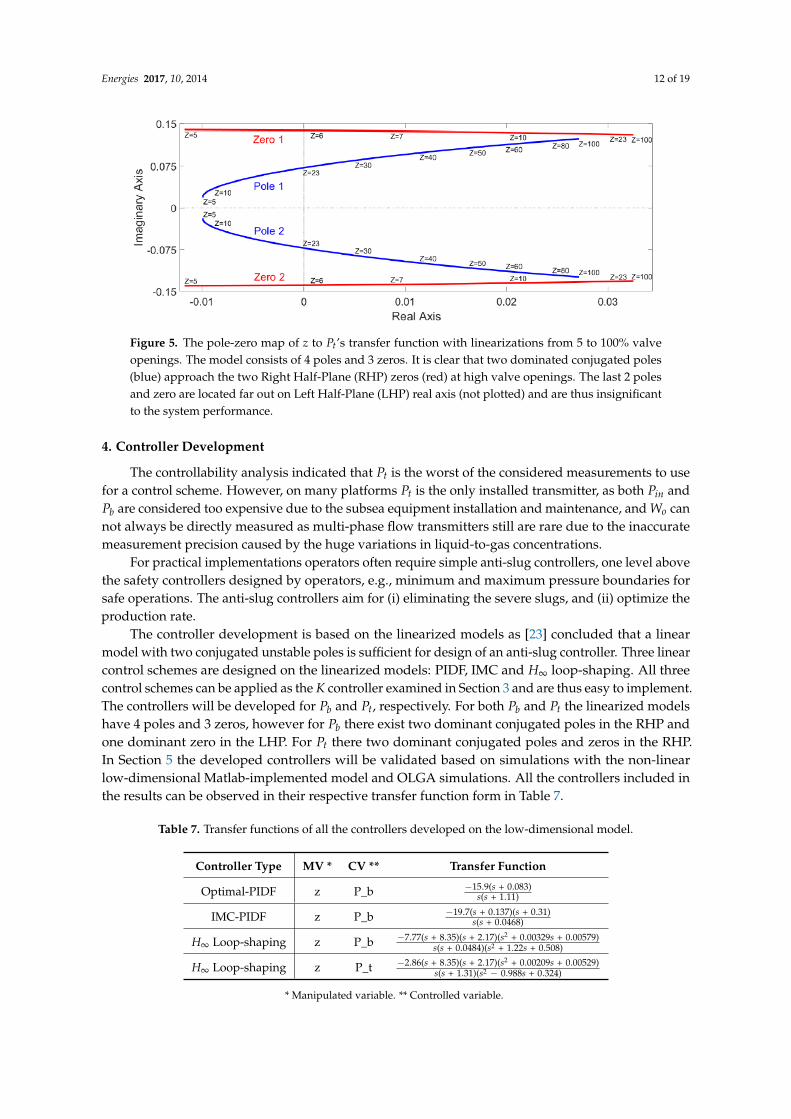
It is clear that Pt in general indicates the worst possible performance, especially for the largeopenings (Z > 45%). It is also observed from ||S||∞,min that only Pt has RHP zeros. Figure 5 shows thepole-zero map of Pt for different valve openings (linearization points). The two dominated conjugatedpoles get closer to two RHP zeros the higher the valve opening is, which is also observed from theTables 3–6. According to Equation (22) the sensitivity function rapidly increases when a RHP poleapproaches a RHP zero. Furthermore ||KS||∞,min and ||SG||∞,min are both larger for Pt which indicatethe system is sensitive to measurement noise and input disturbances. For Pb and Pin the results arealike with only minor deviations from each other; both indicate acceptable properties in general andseem to handle disturbances well. Only for Z = 75% the KS is large and can cause problems for outputnoise and disturbances. Wo seems to be the best solution, although it is the worst measurement for theinduced disturbances in ||KSG1||∞,min, ||KSG2||∞,min and especially ||SG2||∞,min.

In general Pt seems to be the worst solution for control purpose, where the three other alternativesall seem to be acceptable controlled variables. However, all four measurements seems to be able toeliminate the slug and operate beyond the open-loop bifurcation point.

Energies 2017, 10, 2014 11 of 19

Table 3. Model analysis for Z = 30%.

Measurement Equilibrium G(0) Pole Vector ||S||∞,min ||KS||∞,min ||SG||∞,min ||KSGd1||∞,min ||KSGd2||∞,min ||SGd1||∞,min ||SGd2||∞,minPin [bar] 0.36 −2.62 3.67 1.00 0.05 0.00 0.17 0.32 0.00 0.00Pb [bar] 0.35 −2.62 3.73 1.00 0.05 0.00 0.17 0.32 0.00 0.00Pt [bar] 0.04 −2.46 1.05 1.17 0.16 1.42 0.16 0.34 0.23 0.53

ωo [kg/s] 0.18 0.00 156 1.00 0.00 0.00 0.16 0.34 0.03 32.4

Table 4. Model analysis for Z = 45%.

Measurement Equilibrium G(0) Pole Vector ||S||∞,min ||KS||∞,min ||SG||∞,min ||KSGd1||∞,min ||KSGd2||∞,min ||SGd1||∞,min ||SGd2||∞,minPin [bar] 0.36 −1.17 3.60 1.00 0.21 0.00 0.35 0.62 0.00 0.00Pb [bar] 0.34 −1.17 3.73 1.00 0.20 0.00 0.33 0.64 0.00 0.00Pt [bar] 0.03 −1.10 0.58 1.88 1.31 1.44 0.32 0.68 0.23 0.53

ωo [kg/s] 0.18 0.00 192 1.00 0.00 0.00 0.32 0.70 0.03 32.4

Table 5. Model analysis for Z = 60%.

Measurement Equilibrium G(0) Pole Vector ||S||∞,min ||KS||∞,min ||SG||∞,min ||KSGd1||∞,min ||KSGd2||∞,min ||SGd1||∞,min ||SGd2||∞,minPin [bar] 0.35 −0.44 3.58 1.00 0.69 0.00 0.89 1.57 0.00 0.00Pb [bar] 0.34 −0.44 3.76 1.00 0.65 0.00 0.84 1.60 0.00 0.00Pt [bar] 0.03 −0.41 0.36 3.09 6.83 0.97 0.79 1.76 0.23 0.53

ωo [kg/s] 0.18 0.00 212 1.00 0.01 0.00 0.80 1.78 0.03 32.4

Table 6. Model analysis for Z = 75%.

Measurement Equilibrium G(0) Pole Vector ||S||∞,min ||KS||∞,min ||SG||∞,min ||KSGd1||∞,min ||KSGd2||∞,min ||SGd1||∞,min ||SGd2||∞,minPin [bar] 0.35 −0.14 3.57 1.00 2.35 0.00 2.73 4.79 0.00 0.00Pb [bar] 0.34 −0.14 3.78 1.00 2.22 0.00 2.53 4.85 0.00 0.00Pt [bar] 0.03 −0.13 0.24 4.74 34.6 0.48 2.40 5.41 0.23 0.53

ωo [kg/s] 0.18 0.00 223 1.00 0.04 0.00 2.42 5.47 0.03 32.4

Energies 2017, 10, 2014 12 of 19

Figure 5. The pole-zero map of z to Pt’s transfer function with linearizations from 5 to 100% valveopenings. The model consists of 4 poles and 3 zeros. It is clear that two dominated conjugated poles(blue) approach the two Right Half-Plane (RHP) zeros (red) at high valve openings. The last 2 polesand zero are located far out on Left Half-Plane (LHP) real axis (not plotted) and are thus insignificantto the system performance.

4. Controller Development

The controllability analysis indicated that Pt is the worst of the considered measurements to usefor a control scheme. However, on many platforms Pt is the only installed transmitter, as both Pin andPb are considered too expensive due to the subsea equipment installation and maintenance, and Wo cannot always be directly measured as multi-phase flow transmitters still are rare due to the inaccuratemeasurement precision caused by the huge variations in liquid-to-gas concentrations.

For practical implementations operators often require simple anti-slug controllers, one level abovethe safety controllers designed by operators, e.g., minimum and maximum pressure boundaries forsafe operations. The anti-slug controllers aim for (i) eliminating the severe slugs, and (ii) optimize theproduction rate.

The controller development is based on the linearized models as [23] concluded that a linearmodel with two conjugated unstable poles is sufficient for design of an anti-slug controller. Three linearcontrol schemes are designed on the linearized models: PIDF, IMC and H∞ loop-shaping. All threecontrol schemes can be applied as the K controller examined in Section 3 and are thus easy to implement.The controllers will be developed for Pb and Pt, respectively. For both Pb and Pt the linearized modelshave 4 poles and 3 zeros, however for Pb there exist two dominant conjugated poles in the RHP andone dominant zero in the LHP. For Pt there two dominant conjugated poles and zeros in the RHP.In Section 5 the developed controllers will be validated based on simulations with the non-linearlow-dimensional Matlab-implemented model and OLGA simulations. All the controllers included inthe results can be observed in their respective transfer function form in Table 7.

Table 7. Transfer functions of all the controllers developed on the low-dimensional model.

Controller Type MV * CV ** Transfer Function

Optimal-PIDF z P_b −15.9(s + 0.083)s(s + 1.11)

IMC-PIDF z P_b −19.7(s + 0.137)(s + 0.31)s(s + 0.0468)

H∞ Loop-shaping z P_b −7.77(s + 8.35)(s + 2.17)(s2 + 0.00329s + 0.00579)s(s + 0.0484)(s2 + 1.22s + 0.508)

H∞ Loop-shaping z P_t −2.86(s + 8.35)(s + 2.17)(s2 + 0.00209s + 0.00529)s(s + 1.31)(s2 − 0.988s + 0.324)

* Manipulated variable. ** Controlled variable.

Energies 2017, 10, 2014 13 of 19

4.1. Optimal PIDF Controller Design

A Proportional–Integral–Derivative controller with low-pass filter (PIDF) controller has thefollowing structure in the standard form:

KPIDF(s) = Kp(1 +1

sTi+

TdsTf s + 1

) (30)

where Kp is the proportional gain, Ti is the integral time, Td is the derivative time and Tf is the timeconstant of the derivative filter. The filter is essential for reducing the noise effect to the derivative part.

The controller was automatically tuned by using an optimization algorithm to minimize theweighted sum of a cost function (J(t)) for the closed-loop input and output performance, such that theoptimization problem finds the minimum J(t) by manipulating K using the Integrated Square Error(ISE). The cost function in Equation (32) is obtained from applying the cost from the ISE function inEquation (31) and adding an extra cost parameter:

ISE =∫ ∞

0(r(t)− y(t))2dt (31)

minK

J(t) = minK

∫ ∞

0

(wy(r(t)− y(t))2 + wu,di f |u(t)|2

)dt (32)

where r is the output reference, and wy and wu,di f are weighting values. wy is weighted the highestto prioritize the weighting of the output error the most and wu,di f was adjusted to take care of thephysical rate limiter for the choke valves opening speed.

During the tuning it was observed that Ti was problematic as an increased integral gain decreasesthe controllers robustness and heavily influences the oscillations of the system. However with nointegral part the controller will not converge to the given setpoint. Thus a significant high Ti was usedfor Pb. For Pt the controller had problems handling the non-minimum phase system, generated by theRHP zero. In the OLGA simulations it was possible to manually tune a PI controller with large Ti forstabilizing the system without oscillations, but with long settling time.

4.2. IMC Controller Design

Internal Model Control (IMC) includes the model in the control scheme. In this case we designthe controller based on the linearized model. The IMC can also be calculated from

u(s) = K(r− (yp(s)− y(s))) (33)

where yp is the plant’s output and y is the model’s output calculated as y(s) = G(s)u(s) where G is thetransfer function model. The IMC structure is converted into a standard PIDF structure for K wherethe control parameters are tuned based on G. For more information of the structure see [24].

4.3. H-Infinity Loop-Shaping Controller Design

H∞ loop-shaping is based on the perturbed plant model Gp to maximize the stability margin formodel uncertanties. The normalized left coprime factorization of G is

G = M−1N. (34)

For simplification, the subscript of M and N is not included. Hence, the perturbed plant model is

GP = (M +4M)−1(N +4N). (35)

Energies 2017, 10, 2014 14 of 19

Here4M and4N are stable transfer functions which represent the uncertainty in the nominalplant model. The controller’s objective is to stabilize a list of perturbed plants. Hence the closed-loopfeedback system is stable if and only if the nominal feedback system is stable and

γK4=

∥∥∥∥∥[

KI

](I − GK)−1M−1

∥∥∥∥∥∞

≤ 1ε

(36)

where ε > 0 is the stability margin and γK is the H∞ norm. When γK is small the stability margin, ε, iscorrespondingly large.

5. Results and Discussion

In this section the developed controllers’ performances are investigated and compared to eachother. The results are obtained using both laboratory experiments and simulations of the non-linearlow-dimensional model and OLGA model, respectively. The OLGA simulations are included becauseit is more detailed than the low-dimensional model and thus potentially can provide more realisticresults. The numerous obtained results, both from experiments and simulations, are included to givean enhanced overview of the developed controllers’ performances.

5.1. Controller Comparison

The results of the PIDF, IMC and H∞ loop-shaping controllers for two different independentpressure measurements (Pt and Pb) can be observed in Table 8. The table shows the maximum allowedchoke valve openings before the closed-loop systems goes unstable (Zbi f ). The results are based onsimulations with the non-linear model in MATLAB and the OLGA model.

Table 8. Controller comparison between Pb and Pt with optimal PIDF, IMC-PIDF and H∞ loop-shapingcontrol schemes. The table’s result entries show the absolute maximum stable choke opening indicatingthe closed-loop bifurcation point for each controller respectively.

Open-Loop Zbi f = 23% * Non-Linear MATLAB Model OLGA Model

Measurement Optimal IMC-PIDF H∞ Optimal Tuned IMC-PIDF H∞

PIDF Loop-Shaping PIDFMATLAB PIDFOLGA Loop-ShapingPb [bar] 62% 70% 98% 46% 59% ** 47% 74%Pt [bar] - - 35% - 29% ** - 41%

* The open-loop Zbi f is 23.3 % in OLGA and 23.6 % in MATLAB. ** The controller has been retuned in OLGAto obtain better results.

It is clear that Pb gives the best performance for any of the three control schemes respectively,where Pt only can stabilize with relatively low openings in both the MATLAB and OLGA simulations.The open-loop bifurcation point was not improved for Pt with PIDF or IMC controllers, however bymanual tuning in OLGA a PI controller was obtained which could move the bifurcation point to 29%which corresponds to a relative increase of 6%. This solution however, had a slow converge rate asthe integral gain had to be relatively low with respect to the proportional gain to guarantee stability.A similar issue was observed for Pb using the PIDF control scheme, where the the integral gain had tobe significantly smaller than the proportional gain to guarantee stability. Even with a low integral gainthe PIDF controllers resulted in big fluctuations and long settling time for the system.

The best system performance for both Pb and Pt was achieved using the H∞ loop-shapingcontroller which could effectively eliminate the slug with high valve openings both in the MATLABand OLGA simulations. The fastest settling time (≈20 s for Pb at Z = 40% and ≈ 65 s for Pt at Z = 40%)was also obtained with the H∞ loop-shaping controller. This is an acceptable system convergencerate with subject to the open-loop severe slug frequency ( 1

70 Hz). Figures 6 and 7 shows the MATLABsimulations of the closed-loop non-linear system performance using the H∞ loop-shaping controllerwith Pt and Pb respectively. It is clear that the Pt H∞ loop-shaping controller gets worse performanceat high openings where it barely stabilizes the system close to the closed-loop bifurcation point, the Pb

Energies 2017, 10, 2014 15 of 19

H∞ loop-shaping controller operates well at high openings, but the choke valve’s saturation cause thesystem to be unstable in the end.

Figure 6. The non-linear model with the loop-shaping controller for Pt. The setpoint is stepped tofind highest allowed valve opening. At 1000 s the system stabilizes at highest allowed opening beforereaching the closed-loop bifurcation point.

Figure 7. The non-linear model with the loop-shaping controller for Pb. The setpoint is stepped tofind highest allowed valve opening. At 1000 s the system cannot stabilize due to the saturation of thechoke valve.

5.2. Control with Model Disturbances

Disturbances have been introduced to the model to further evaluate the closed-loop systemperformances with the considered controllers.

Energies 2017, 10, 2014 16 of 19

The mass flow inputs, wg,in (u2) and wl,in (u3), are often only estimated on real platforms as flowtransmitters not always are installed at the pipeline inlet. Thus the robustness of the controllers havebeen examined with input disturbance simulations in MATLAB, see Table 9. The input disturbancesvary from the linearization points of the model at which the controller designs are based on. Note thatthe input disturbances included are negative (lower inlet mass flow), as it is experienced that systemswith lower flow rates (especially for lower wg,in) are harder for the controller to stabilize. The resultsshow that the H∞ loop-shaping controller overall handles the disturbances the best. The Pt H∞

loop-shaping controller handles the disturbances well, but performs significantly worse when wg,inis low. For the Pb the H∞ loop-shaping controller can still operate with large valve opening evenwith disturbances. The IMC-PIDF controller performed aggressively to stabilize the system, howevera rate limiter was included in the simulations to emulate the valve’s opening speed. This causedthe IMC-PIDF controller performance to decrease, especially for the larger steps in the setpoint.The optimal PIDF controller had an overall inadequate settling time and was considered inferior to theevaluated Pb controllers.

The identified low-dimensional model is based on 2-phase flow, where the gas is air and the liquidis water. In reality the liquid phase consists of a mixture of water and crude oil, and the gas phase ismethane, ethane, propane, carbon dioxide and hydrogen sulfide etc. It has to be noted that most fluidsare in liquid phases in the reservoir, but phase changes can occur when the high pressure is reducedthroughout the transportation pipeline. The different compositions can be considered in the modelby varying the densities and viscosities. A bigger ratio of crude oil will reduce the density whichcorrespondingly reduces the slug cycle amplitude and increases the slug cycle frequency. However theincrease in crude oil also significantly increases the viscosity, which has huge impact on the friction.Table 9 include these parametric disturbances where the change in compositions are listed. For both Pband Pt the controllers in general handles the disturbances well; The PIDF controller’s performance isstill below the performance of the H∞ loop-shaping technique which is the preferred method.

The system response is acceptable for all three Pb controllers, but the settling time is low for theoptimal PIDF controller where no overshoot is included due to the low integral gain. The IMC-PIDFcontroller gives the fastest settling time in some scenarios but worst for others. The loop-shapingcontroller is the most robust and can operate with large valve openings, even for huge disturbances.For the Pt controller the performance is very uniform over most disturbances, however for somevariations the controller was not able to stabilize the system above the open-loop bifurcation point.

Table 9. Controller comparison between Pb and Pt with input and parametric disturbances based onnon-linear MATLAB simulations. The result entries show the new bifurcation points for each disturbedsystem with the controllers from Table 8.

Non-Linear MATLAB Model Properties Pb Pt

Disturbances Open-Loop Optimal IMC-PIDF H∞ H∞

Zbi f PIDFMATLAB Loop-Shaping Loop-Shaping−3% wg,in 22% 47% 60% 98% 33%−6% wg,in 21% 40% 38% 75% -−3% wl,in 24% 61% 65% 94% 32%−6% wl,in 25% 60% 64% 91% 31%

−3% wg,in, −3% wl,in 23% 37% 38% 92% 32%−6% wg,in, −6% wl,in 23% 36% 35% 87% -

15 ◦C, Woil/Wwater = 0.25 26% 55% 68% 98% 34%15 ◦C, Woil/Wwater = 0.50 31% 70% 70% 98% 34%40 ◦C, Woil/Wwater = 0.25 28% 35% 72% 70% 34%40 ◦C, Woil/Wwater = 0.50 39% 61% 82% 98% -

6. Conclusions and Future Work

This paper examines the model analysis and control design of several anti-slug controllers.The work focuses on linear controllers based on the linearized slug models but tested against the

Energies 2017, 10, 2014 17 of 19

non-linear low-dimensional and OLGA models. The linearized model analysis gave an indication ofwhich controlled variables are preferable and it was concluded that the low-point measurements arepreferable over the topside transmitters where the topside flow transmitter is the best alternative ifonly topside measurements are available.

Slug modeling is a difficult task and it is experienced that the MATLAB and OLGA modelsdid not fit the lab data perfectly in every aspect. The MATLAB model’s accuracy was improvedby some modifications: A change in Darcy friction, an added top pressure for better estimating ωo,an updated static valve characteristic for f (z), and a new tuning parameter for the estimating howmuch liquid is leaving the riser during a slug’s blowout stage. Even with these modifications, modeldeviations were still present, especially in the amplitude of Pt during slug flow. However, this is alsothe case for the OLGA model. Furthermore, even though deviations from the reality exist, both theMATLAB and OLGA model are very accurate on most parameters, such as: the open-loop bifurcationpoint, equilibrium pressure and transient performance. Besides, the OLGA and MATLAB simulationsgave consistent results. The main limitation of including the MATLAB model’s modifications, is theapplicability, which to some degree compromised with more tuning parameters and extra equations.

The control solutions were based on the riser top and bottom pressures as these are the mostcommon transmitters on offshore platforms. A comparison between optimal PIDF, IMC-PIDF and H∞

loop-shaping controllers were carried out based on the non-linear low-dimensional MATLAB modeland on OLGA simulations. Pb archieved acceptable performance with all three controllers in both thenon-linear MATLAB and OLGA simulations. In MATLAB only the H∞ loop-shaping control techniquewas able to stabilize the system above the open-loop bifurcation point using the Pt as the controlledvariable, although Pt H∞ loop-shaping still had a relatively low Zbi f . In OLGA it was possible tofind a PI controller for Pt which could stabilize the system just above the open-loop bifurcation point,although the system had a long settling time due to the low integral gain required for stabilizing thesystem. Furthermore, the controllers was examined with input and parametric system disturbances,where the H∞ loop-shaping technique once again proved to be the best of the considered controllerdue to the controller’s ability to handle uncertain systems. For Pt the controller was able to handle thedisturbances in most cases but was still only able to operate with relatively low valve openings.

It is concluded the Pb is the preferable pressure transmitter to use for feedback control in ananti-slug control scheme. However, if only the topside pressure transmitter is available this canstill be used for eliminating the slug outside the open-loop slug region. The H∞ loop-shapingcontrol solution gave the best performance for both Pb and Pt. For a slug model a robust controller(such as H∞ loop-shaping) seems to handle the uncertain running conditions much better than anoptimal controller (such as optimal PIDF), and furthermore the robustness does not sacrifice muchof the control performance. The biggest limitation using the H∞ loop-shaping controllers are thesignificant overshoots at the output transient response before output stabilization. In future workfurther evaluation of the controllers’ performance will be based on implementations on the lab-scaledtesting rig. This has not been possible as the testing facility has been further modified after the systemidentification data was obtained, and thus the model has to be updated and re-identified with the newfacility dimensions.

Acknowledgments: The authors would like to thank the support from the Innovation Foundation (via PDPWACProject (J.nr. 95-2012-3)). Thanks also to our colleagues from Norwegian University of Science andTechnology, Aalborg University, Maersk Oil A/S, Ramboll Oil & Gas A/S, for many valuable discussions andtechnical supports.

Author Contributions: Sigurd Skogestad and Zhenyu Yang suggested and facilitated the tools applied forthe model analysis and controller development. Simon Pedersen designed and performed the experiments.Simon Pedersen and Esmaeil Jahanshahi made the model modifications and simulations. Esmaeil Jahanshahi,Zhenyu Yang and Sigurd Skogestad reviewed the paper. Simon Pedersen wrote the paper.

Conflicts of Interest: The authors declare no conflict of interest.

Energies 2017, 10, 2014 18 of 19

References

1. Pedersen, S.; Durdevic, P.; Yang, Z. Challenges in slug modeling and control for offshore oil and gasproductions: A review study. Int. J. Multiph. Flow 2017, 88, 270–284.

2. Hill, T.J.; Wood, D.G. Slug flow: Occurrence, consequences, and prediction. In Proceedings of the Universityof Tulsa Centennial Petroleum Engineering Symposium, Tulsa, Oklahoma, 29–31 August 1994.

3. Havre, K.; Stornes, K.O.; Stray, H. Taming slug flow in pipelines. ABB Rev. 2000, 4, 55–63.4. Havre, K.; Dalsmo, M. Active Feedback Control as the Solution to Severe Slugging. In Proceedings of the

SPE Annual Technical Conference & Exhibition, San Antonio, TX, USA, 9–11 October 2017.5. Ogazi, A.I. Multiphase Severe Slug Flow Control. Ph.D. Thesis, School of Engineering, Department of

Offshore, Process and Energy Engineering, Cranfield University, Cranfield, UK, 2011.6. Jahanshahi, E. Control Solutions for Multiphase Flow—Linear and Nonlinear Approaches to Anti-Slug

Control. Ph.D. Thesis, Norwegian University of Science and Technology, Trondheim, Norway, 2013.7. Hu, B. Characterizing Gas-Lift Instabilities. Ph.D. Thesis, Norwegian University of Science and Technology

(NTNU), Trondheim, Norway, 2004.8. Jepsen, K.; Hansen, L.; Mai, C.; Yang, Z. Emulation and Control of Slugging Flows in a Gas-Lifted Offshore

Oil Production Well Through a Lab-sized Facility. In Proceedings of the IEEE International Conference onControl Applications (CCA), Hyderabad, India, 28–30 August 2013; pp. 906–911.

9. Jansen, F.E.; Shoham, O.; Taitel, Y. The Elimination of severe slugging - experiments and modeling. Int. J.Multiph. Flow 1996, 22, 1055–1072.

10. Ogazi, A.; Cao, Y.; Yeung, H.; Lao, L. Slug Control With Large Valve Openings To Maximize Oil Production.SPE J. 2010, 15, 3.

11. Pedersen, S.; Durdevic, P.; Yang, Z. Learning control for riser-slug elimination and production-rateoptimization for an offshore oil and gas production process. In Proceedings of the 19th World Congress of theInternational Federation of Automatic Control, Cape Town, South Africa, 24–29 August 2014; pp. 8522–8527.

12. De Oliveira, V.; Jäschka, J.; Skogestad, S. An Autonomous Approach for Driving Systems towards TheirLimit: An Intelligent Adaptive Anti-Slug Control System for Production Maximization. In Proceedings ofthe 2nd IFAC Workshop on Automatic Control in Offshore Oil and Gas Production, Florianopolis, Brazil,27–29 May 2015; pp. 104–111.

13. Jahanshahi, E.; Skogestad, S.; Helgesen, A.H. Controllability analysis of severe slugging in well-pipeline-risersystems. In Proceedings of the IFAC Workshop on Automatic Control in Offshore Oil and Gas Production,NTNU, Trondheim, Norway, 31 May–1 June 2012; pp. 101–108.

14. Jahanshahi, E.; Oliveira, V.D.; Grimholt, C.; Skogestad, S. A comparison between Internal Model Control,optimal PIDF and robust controllers for unstable flow in risers. In Proceedings of the 19th World Congress,The International Federation of Automatic Control (IFAC’14), Cape Town, South Africa, 24–29 August 2014;pp. 5752–5759.

15. Jahanshahi, E.; Skogestad, S. Simplified Dynamic Models for Control of Riser Slugging in Offshore Oil Production;SPE 172998; Society of Petroleum Engineers: Richardson, TX, USA, 2014; pp. 40–55.

16. Drew, T.B.; Koo, E.C.; McAdams, W.H. The Friction Factor for Clean Round Pipes. Trans. AIChe 1932, 28,56–72.

17. Haaland, S.E. Simple and Explicit Formulas for the Friction Factor in Turbulent Flow. J. Fluids Eng. (ASME)1983, 105, 89–90.

18. Biltoft, J.; Hansen, L.; Pedersen, S.; Yang, Z. Recreating Riser Slugging Flow Based on an Economic Lab-sizedSetup. In Proceedings of the 5th IFAC International Workshop on Periodic Control Systems, Caen, France,3–5 July 2013; pp. 47–52.

19. Pedersen, S. Plant-Wide Anti-Slug Control for Offshore Oil and Gas Processes. Ph.D. Thesis, Aalborg University,Aalborg, Denmark, 2016.

20. Meglio, F.D.; Petit, N.; Alstadb, V.; Kaasab, G.O. Stabilization of slugging in oil production facilities with orwithout upstream pressure sensors. J. Process Control 2012, 22, 809–822.

21. Skogestad, S.; Postlethwaite, I. Multivariable Feedback Control: Analysis and Design; Wiley & Sons: Hoboken,NJ, USA, 2005.

22. Chen, J. Logarithmic integrals, interpolation bounds and performance limitations in MIMO feedback systems.IEEE Trans. Autom. Control 2000, 45, 1098–1115.

Energies 2017, 10, 2014 19 of 19

23. Jahanshahi, E.; Skogestad, S. Closed-loop model identification and PID/PI tuning for robust antislug control.In Proceedings of the 10th IFAC International Symposium on Dynamics and Control of Process Systems,Mumbai, India, 18–20 December 2013; pp. 233–240.

24. Jahanshahi, E.; Skogestad, S. Anti-slug control solutions based on identified model. J. Process Control 2015,30, 58–68.

c© 2017 by the authors. Licensee MDPI, Basel, Switzerland. This article is an open accessarticle distributed under the terms and conditions of the Creative Commons Attribution(CC BY) license (http://creativecommons.org/licenses/by/4.0/).