Comparison of Automatic Image Contrast … of Automatic Image Contrast Enhancement Using ... of an input image or wavelet transform of an input image. ... uses a small window that

International Journal of Computer Science Trends and Technology (IJCST) – Volume 2 Issue 5, Sep-Oct 2014

ISSN: 2347-8578 www.ijcstjournal.org Page 89

Comparison of Automatic Image Contrast Enhancement Using

Gaussian Mixture Model and Global Histogram Equalization M. Muni sankar1, R.Sankeerthana2, CH. Nageswara Rao3

*Academic Consultant1&2, Assistant professor3

Department of Electronics and Communication Engineering

Sri Padmavathi Mahila Visvavidhyalayam1&2, Thirupathi SIST3, Puttur

A.P - India

ABSTRACT In this project, we have implemented Image Contrast Enhancement algorithm that automatically enhances the contrast in an input

image. The algorithm uses the Gaussian mixture model to model the image gray-level distribution and the intersection points of the

Gaussian components in the model are used to partition the dynamic range of the image into input gray-level intervals. The contrast

equalized image is generated by transforming the pixels’ gray levels in each input interval to the appropriate output gray-level

interval according to the dominant Gaussian component and the cumulative distribution function of the input interval. To take

account of the hypothesis that homogeneous regions in the image represent homogeneous silences (or set of Gaussian components)

in the image histogram, the Gaussian components with small variances are weighted with smaller values than the Gaussian

components with larger variances, and the gray-level distribution is also used to weight the components in the mapping of the input

interval to the output interval. Experimental results show that the proposed algorithm produces better or comparable enhanced

images than state-of-the-art algorithms like GHE. Unlike the other algorithms, the proposed algorithm is free of parameter setting

for a given dynamic range of the enhanced image and can be applied to a wide range of image types. Keywords:- Image enhancement system, Gaussian mixture model. Histogram specific enhancement, brightness-preserving

histogram equalization with maximum entropy, minimum mean brightness error bi-histogram equalization

I. INTRODUCTION

Digital image processing is the use of computer

algorithms to perform image processing on digital images.

As a subcategory or field of digital signal processing, digital

image processing has many advantages over analog image

processing. It allows a much wider range of algorithms to be

applied to the input data and can avoid problems such as the

build-up of noise and signal distortion during processing.

Since images are defined over two dimensions (perhaps

more) digital image processing may be modelled in the form

of multidimensional systems.

In imaging science, image processing is any form of

signal processing for which the input is an image, such as a

photograph or video frame; the output of image processing

may be either an image or a set of characteristics or

parameters related to the image. Most image-processing

techniques involve treating the image as a two-dimensional

signal and applying standard signal-processing techniques to

it. Image processing usually refers to digital image

processing, but optical and analog image processing also are

possible. This article is about general techniques that apply to

all of them. The acquisition of images (producing the input

image in the first place) is referred to as imaging.

Image enhancement is refers to accentuation, or

sharpening, of image features such as boundaries, or contrast

to make a graphic display more useful for display & analysis.

This process does not increase the inherent information

content in data. It includes gray level & contrast

manipulation, noise reduction, edge christenings and

sharpening, filtering, interpolation and magnification, pseudo

colouring, and so on.

Image enhancement is designed to emphasize

features of the image that make the image more pleasing to

the observer. It is the process of improving the quality of a

digitally stored image by manipulating it. Image

enhancement is used in various important fields such as

medical image diagnosis, finger print recognition,

photography enhancement, satellite imagery. Image

enhancement is mainly used for improving visibility of

pictures and for feature recognition. Contrast enhancement is

a common operation in image processing. It's a useful

method for processing scientific images such as X-Ray

images or satellite images. And it is also useful to improve

detail in photographs that are over or under-exposed.

Image enhancement system:

The enhancement system could be a spatial domain

RESEARCH ARTICLE OPEN ACCESS

http://www.ijcstjournal.org/



where manipulation with direct image pixels or could be

frequency domain where manipulation of Fourier transform

of an input image or wavelet transform of an input image.

The reason for enhancement is to attenuate the effects of sub-

sampling, to attenuate quantization effects, to remove noise

and simultaneously preserve edges and image details, and to

avoid aliasing effects, to attenuate the blackness effect and to

enhancement special features to be more easily detected by a

machine or a human observer.

The brief introduction of GMM:

Image modelling is one of the important phases in

image enhancement. For image modelling, Gaussian Mixture

Model (GMM) is the standard methodology. Gaussian

mixture model has been widely used in fields of pattern

recognition, information processing and data mining. If the

number of the Gaussians in the mixture is pre-known, the

well-known Expectation-Maximization (EM) algorithm

could be used to estimate the parameters in the Gaussian

mixture model.

Image contrast enhancement using Gaussian mixture

modelling is an effective in terms of improving the visual

quality of different types of input images. Images with low

contrast are automatically improved in terms of an increase

in the dynamic range. Images with sufficiently high contrast

are also improved but not as much. Firstly the pixel values of

an input image are modelled using the Gaussian mixture

model (GMM).The intersection points of the Gaussian

components are used in partitioning the dynamic range of the

input image into different intervals. The pixels in each input

interval are transformed to the output interval according to

the dominant Gaussian component and the CDF of the input

interval.

The objective of the project:

The main objective of an image enhancement

technique is

To bring out hidden image details

To increase the gray level differences among objects

and background

To increase the dynamic range of an image with a

low dynamic range.

To generate an enhanced image, which has a better

visual quality with respect to input image.

II. LITERATURE SURVEY

Image enhancement is required mostly for better

visualization or rendering of images to aid our visual

perception. There are various reasons, why a raw image data

requires processing before display. The dynamic range of the

intensity values may be small due to the presence of strong

background illumination, as well as due to the insufficient

lighting. It may be the other way also. The dynamic range of

the original image may be too large to be accommodated by

limited number of bit-planes of a display device. The

problem gets more complicated when the illumination of the

scene widely varies in the space focused on the enhancement

of gray-level images in the spatial domain. These methods

include adaptive histogram equalization, unsharp masking,

constant variance enhancement, homomorphic filtering, high-

pass, and low-pass filtering, etc.

Enhancement techniques:

Numerous enhancement techniques have been

introduced and these can be divided into three groups:

1) Techniques that decompose an image into high and low

frequency signals for manipulation [3], [4];

2) Transform-based techniques [5]; and

3) Histogram modification techniques [6]–[17].

Techniques in the first two groups often use

multiscale analysis to decompose the image into different

frequency bands and enhance its desired global and local

frequencies. These techniques are computationally complex

but enable global and local contrast enhancement

simultaneously by transforming the signals in the appropriate

bands or scales. Furthermore, they require appropriate

parameter settings that might otherwise result in image

degradations. For example, the centre-surround Retinex [2]

algorithm was developed to attain lightness and colour

constancy for machine vision applications. The constancy

refers to the resilience of perceived colour and lightness to

spatial and spectral illumination variations. The benefits of

the Retinex algorithm include dynamic range compression

and colour independence from the spatial distribution of the

scene illumination. However, this algorithm can result in

“halo” artefacts, particularly in boundaries between large

uniform regions. Moreover, “greying out” can occur, in

which the scene tends to change to middle gray.

Among the three groups, the third group received the

most attention due to their straightforward and intuitive

implementation qualities. Linear contrast stretching (LCS)

and global histogram equalization (GHE) are two widely

utilized methods for global image enhancement. The former

linearly adjusts the dynamic range of an image, and the latter

uses an input to output mapping obtained from the

cumulative distribution function (CDF), which is the integral

of the image histogram. Since the contrast gain is

proportional to the height of the histogram, gray levels with

large pixel populations are expanded to a larger range of gray

levels, whereas other gray-level ranges with fewer pixels are

compressed to smaller ranges. Although GHE can efficiently




utilize display intensities, it tends to over enhance the image

contrast if there are high peaks in the histogram, often

resulting in a harsh and noisy appearance of the output

image. LCS and GHE are simple transformations, but they do

not always produce good results, particularly for images with

large spatial variation in contrast. In addition, GHE has the

undesired effect of overemphasizing any noise in an image.

In order to overcome the aforementioned problems,

local histogram-equalization (LHE)-based enhancement

techniques have been proposed, e,g.,[6] and [7]. For example,

the LHE method [7] uses a small window that slides through

every image pixel sequentially, and only pixels within the

current position of the window are histogram equalized; the

gray-level mapping for enhancement is done only for the

centre pixel of the window. Thus, it utilizes local

information. However, LHE sometimes causes over

enhancement in some portion of the image and enhances any

noise in the input image, along with the image features.

Furthermore, LHE-based methods produce undesirable

checkerboard effects.

Histogram specification (HS) [2] is a method that

uses a desired histogram to modify the expected output-

image histogram. However, specifying the output histogram

is not a straightforward task as it varies from image to image.

The dynamic HS (DHS) [8] generates the specified histogram

dynamically from the input image. In order to retain the

original histogram features, DHS extracts the differential

information from the input histogram and incorporates extra

parameters to control the enhancement such as the image

original value and the resultant gain control value. However,

the degree of enhancement achievable is not significant.

Some research works have also focused on

improving histogram-equalization-based contrast

enhancement such as mean preserving bihistogram

equalization (BBHE) [9], equal-area dualistic sub image

histogram equalization (DSIHE), and minimum mean-

brightness (MB) error bihistogram equalization

(MMBEBHE) [11]. BBHE first divides the image histogram

into two parts with the average gray level of the input-image

pixels as the separation intensity. The two histograms are

then independently equalized. The method attempts to solve

the brightness preservation problem. DSIHE uses entropy for

histogram separation. MMBEBHE is the extension of BBHE,

which provides maximal brightness preservation. Although

these methods can achieve good contrast enhancement, they

also generate annoying side effects depending on the

variation in the gray-level distribution [8]. Recursive mean-

separate histogram equalization [11] is another improvement

of BBHE. However, it is also not free from side effects.

Dynamic histogram equalization (DHE) [13] first smoothens

the input histogram by using a 1-D smoothing filter. The

smoothed histogram is partitioned into sub histograms based

on the local minima. Prior to equalizing the sub histograms,

each sub histogram is mapped into a new dynamic range. The

mapping is a function of the number of pixels in each sub

histogram; thus, a sub histogram with a larger number of

pixels will occupy a bigger portion of the dynamic range.

However, DHE does not place any constraint on maintaining

the MB of the image. Furthermore, several parameters are

used, which require appropriate setting for different images.

Optimization techniques have been also employed

for contrast enhancement. The target histogram of the

method, i.e., brightness-preserving histogram equalization

with maximum entropy (BPHEME) [13], has the maximum

differential entropy obtained using a vibrational approach

under the MB constraint. Although entropy maximization

corresponds to contrast stretching to some extent, it does not

always result in contrast enhancement [15]. In the flattest HS

with accurate brightness preservation (FHSABP) [15],

convex optimization is used to transform the image

histogram into the flattest histogram, subject to a MB

constraint. An exact HS method is used to preserve the image

brightness. However, when the gray levels of the input image

are equally distributed, FHSABP behaves very similar to

GHE. Furthermore, it is designed to preserve the average

brightness, which may produce low contrast results when the

average brightness is either too low or too high. In histogram

modification framework (HMF), which is based on histogram

equalization, contrast enhancement is treated as an

optimization problem that minimizes a cost function [16].

Penalty terms are introduced in the optimization in order to

handle noise and black/white stretching. HMF can achieve

different levels of contrast enhancement through the use of

different adaptive parameters. These parameters have to be

manually tuned according to the image content to achieve

high contrast. In order to design a parameter-free contrast

enhancement method, genetic algorithm (GA) is employed to

find a target histogram that maximizes a contrast measure

based on edge information [17]. We call this method contrast

enhancement based on GA (CEBGA). CEBGA suffers from

the drawbacks of GA-based methods, namely, dependence on

initialization and convergence to a local optimum.

Furthermore, the mapping to the target histogram is scored

by only maximum contrast, which is measured according to

average edge strength estimated from the gradient

information. Thus, CEBGA may produce results that are not

spatially smooth. Finally, the convergence time is

proportional to the number of distinct gray levels of the input

image.

Brief review on related ieee papers:

[12] M. Abdullah-Al-Wadud, M. Kabir, M. Dewan, and O.

Chae, “A dynamic histogram equalization for image contrast




enhancement,” IEEE Trans. Consum.Electron., vol. 53, no. 2,

pp. 593–600, May 2007.

In this paper, a novel contrast enhancement

algorithm is proposed. The proposed approach enhances the

contrast without losing the original histogram characteristics,

which is based on the histogram specification technique. It is

expected to eliminate the annoying side effects effectively by

using the differential information from the input histogram.

The experimental results show that the proposed dynamic

histogram specification (DHS) algorithm not only keeps the

original histogram shape features but also enhances the

contrast effectively. Moreover, the DHS algorithm can be

applied by simple hardware and processed in real-time

system due to its simplicity.

[14] C. Wang, J. Peng, and Z. Ye, “Flattest histogram

specification with accurate brightness preservation,” IET

Image Process., vol. 2, no. 5, pp. 249–262, Oct. 2008.

This method uses convex optimization to transform

the image histogram into the flattest histogram, subject to a

MB constraint. An exact HS method is used to preserve the

image brightness. It is also designed to preserve the average

brightness, which may produce low contrast results when the

average brightness is either too low or too high.

[15] T. Arici, S. Dikbas, and Y. Altunbasak, “A histogram

modification framework and its application for image

contrast enhancement,” IEEE Trans. Image Process., vol. 18,

no. 9, pp. 1921–1935, Sep. 2009.

In this, contrast enhancement is posed as an

optimization problem that minimizes a cost function. It is

used to handle noise and black/white stretching. This method

can achieve different levels of contrast enhancement through

the use of different adaptive parameters. The parameters have

to be manually tuned according to the image content to

achieve high contrast which is a disadvantage.

The aforementioned techniques may create problems

when enhancing a sequence of images, when the histogram

has spikes, or when a natural-looking enhanced image is

required.

In this paper, an image contrast enhancement

algorithm is implemented that automatically enhances the

contrast of image in an effective manner. The first step of

algorithm is to model the image and for this, EM clustering

algorithm is used to model the image which is faster and

effective. After modelling, intersection points of Gaussian

components are used to partition the image into different

intervals. Then the image is generated by transforming the

pixels in each input interval to the appropriate output interval

according to the dominant Gaussian component and the

cumulative distribution function of the input interval. The

Gaussian components with small variances are weighted with

smaller values than the Gaussian components with larger

variances, and the gray-level distribution is also used to

weight the components in the mapping of the input interval to

the output interval.

Advantages:

Simple and more effective.

Provide better enhancement.

Disadvantages:

Require appropriate parameter settings that might otherwise

result in image degradations.

III. GAUSSIAN MIXTURE MODELING

An image enhancement algorithm using GMM

automatically enhances the contrast in an input image. The

algorithm uses the Gaussian mixture model to model the

image gray-level distribution, and the intersection points of

the Gaussian components in the model are used to partition

the dynamic range of the image into input gray-level

intervals. The contrast equalized image is generated by

transforming the pixels’ gray levels in each input interval to

the appropriate output gray-level interval according to the

dominant Gaussian component and the cumulative

distribution function of the input interval. To take account of

the hypothesis that homogeneous regions in the image

represent homogeneous silences (or set of Gaussian

components) in the image histogram, the Gaussian

components with small variances are weighted with smaller

values than the Gaussian components with larger variances,

and the gray-level distribution is also used to weight the

components in the mapping of the input interval to the output

interval.

While using Gaussian mixture modelling EM

algorithm is used to partition or cluster the image for

grouping objects, clustering. Again all objects need to be

represented as a set of numerical features. In addition the user

has to specify the number of groups (referred to as k) he

wishes to identify. Each object can be thought of as being

represented by some feature vector in an n dimensional

space, n being the number of all features used to describe the

objects to cluster. The algorithm then randomly chooses k

points in that vector space, these point serve as the initial

centres of the clusters. Afterwards all objects are each

assigned to centre they are closest to. Usually the distance

measure is chosen by the user and determined by the learning

task. After that, for each cluster a new centre is computed by

averaging the feature vectors of all objects assigned to it. The

process of assigning objects and recomposing centres is

repeated until the process converges. The EM algorithm can

be proven to converge after a finite number of iterations.




Several tweaks concerning distance measure, initial centre

choice and computation of new average centres have been

explored, as well as the estimation of the number of clusters

k. Yet the main principle always remains the same.

The GMM algorithm have three steps.

Modelling: Here GMM is using to partition the distribution

of the input image into a mixture of different Gaussian

components. The data within each interval are represented by

a single Gaussian component that is dominant with respect to

the other components.

Partitioning: The numerical values of the intersection points

between GMM components are determined using an

equation. The consecutive pairs of significant intersection

points are used to partition the dynamic range of the input

image.

Mapping: In mapping, each interval covers a certain range,

which is proportional to weight. In the final mapping of pixel

values from the input interval onto the output interval, the

CDF of the distribution in the output interval is preserved.

The flow chart of the proposed paper

In this project, the GMM technique includes three steps

namely: a) Image modelling, b) partitioning and c) mapping.

For image modelling, GMM is used to partition the

distribution of the input image into a mixture of different

Gaussian components. The data within each interval are

represented by a single Gaussian component that is dominant

with respect to the other components. In the second step,

partitioning the numerical values of the intersection points

between GMM components are determined using an

equation. The consecutive pairs of significant intersection

points are used to partition the dynamic range of the input

image. At last in mapping, each interval covers a certain

range, which is proportional to weight. In the final mapping

of pixel values from the input interval onto the output

interval, the CDF of the distribution in the output interval is

preserved.

Modelling:

A GMM can model any data distribution in terms of a linear

mixture of different Gaussian distributions with different

parameters. Each of the Gaussian components has a different

mean, standard deviation, and proportion (or weight) in the

mixture model. A Gaussian component with low standard

deviation and large weight represents compact data with a

dense distribution around the mean value of the component.

When the standard deviation becomes larger, the data is

dispersed about its mean value. The human eye is not

sensitive to small variations around dense data but is more

sensitive to widely scattered fluctuations. Thus, in order to

increase the contrast while retaining image details, dense data

with low standard deviation should be dispersed, whereas

scattered data with high standard deviation should be

compacted. This operation should be done so that the gray-

level distribution is retained. In order to achieve this, we use

the GMM to partition the distribution of the input image into

a mixture of different Gaussian components.

The grey level distribution , where , of

the input image can be modelled as a density function

composed of a linear combination of functions using the

GMM [18], i.e.,

Input Image

Gray Level Distribution

Finding Parameters

Gaussian Components

Intersection Points

Significant Intersection Points

Dominant Gaussian Components

Calculation of Weight

Output Intervals from Input Intervals

Finding Parameters for Output Intervals

Transformation based on Gaussian Components (Mapping)

Output Image




Where p(x│w_n ) is the nth component density and P(w_n) is the

prior probability of the data points generated from component w_n of the

mixture. The component density functions constrained to be Gaussian

distribution functions, given in equation (2)

where and are the mean and the variance of the

th component, respectively. Each of the Gaussian

distribution functions satisfies the following constraint:

The prior probabilities are chosen to satisfy the following

Constraints:

A GMM is completely specified by its parameters

{ }. The estimation of the probability

distribution function of an input-image data reduces to

finding the appropriate values of . In order to estimate,

maximum-likelihood-estimation techniques such as the

Expectation Maximization (EM) algorithm have been widely

used.

The EM algorithm starts from an initial guess for the

distribution parameters and the log-likelihood is guaranteed

to increase on each iteration until it converges.

EM algorithm:

EM algorithm is based on the interpretation of as

incomplete data pixels i.e., . For

Gaussian Mixtures, the missing part is a set of labels

associated with the pixels,

indicating which component produced each pixel.

is the group label of data point . Where each

label is , where and

for means that data pixel was produced by

component.

Example: data pixel is in

group1

data pixel is in group4 and so

on.

As we are in clustering setting X is given and Z is

unknown, now the complete log likelihood corresponding to

a k-component mixture is

Each was generated by randomly choosing

from , and then was drawn from one of

Gaussians. The parameters of our model are

.

The EM algorithm produces a sequence of estimates

by alternating applying two steps (until some

convergence criterion is met)

E-step: Computes the conditional expectation of the

complete log-likelihood, given and the current estimate

.Since is linear with respect to the missing,

we simply have to compute the conditional

expectation , and plug it into .

The result is so called Q-function. Expectation and

maximization to improve our estimates of ,

Z continue iterating until converged.

Now we have parameters for all

Gaussian components (here we have N=4 no. of groups/

Gaussian components)

Figure 3.1: Gray Level Image Figure 3.2: Gray level Image histogram for figure 3.1 and its GMM fit




The selection of (partly) determines where the

algorithm converges or hits the boundary of the parameter

space to produce singular results. Furthermore, the EM

algorithm requires the user to set the number of components,

and the number is fixed during the estimation process.

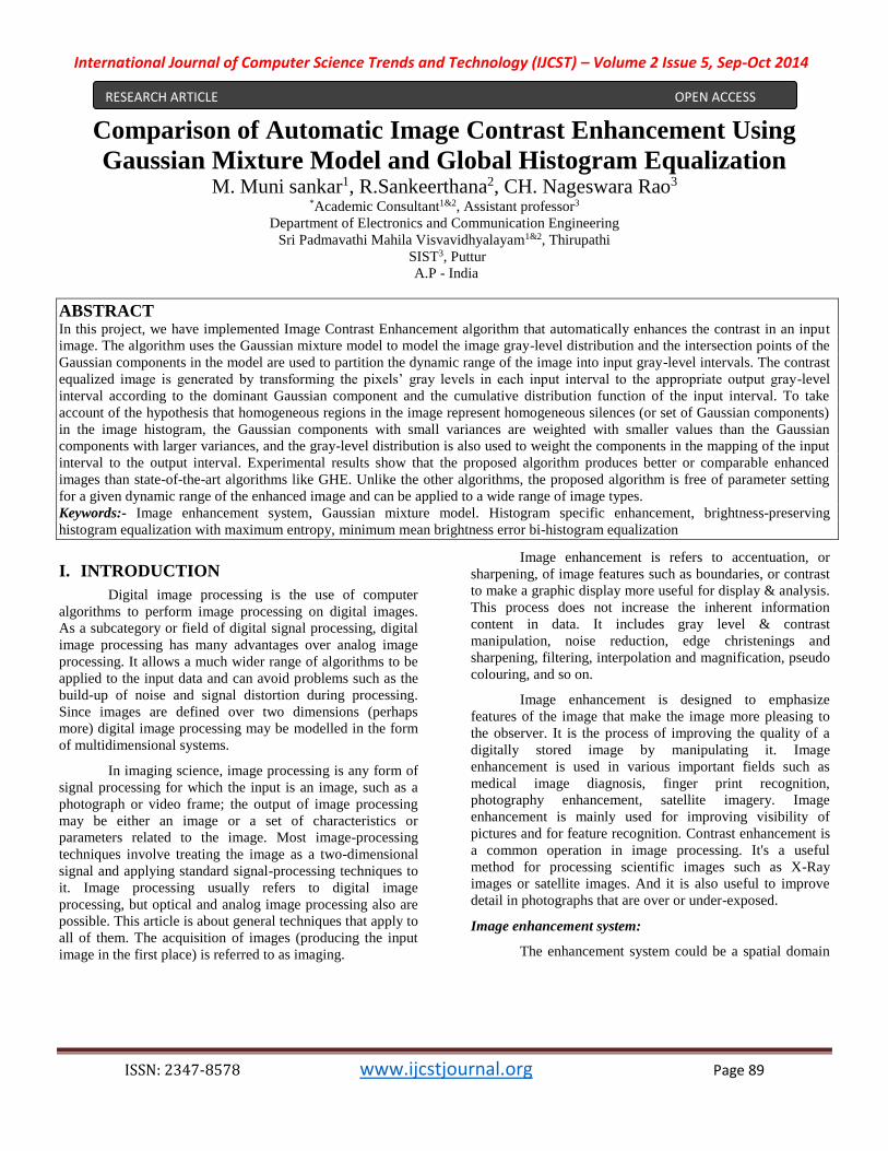
Fig. 3.1 and Fig 3.2 illustrates an input image and its

histogram, together with its GMM fit, respectively The

histogram is modeled using four Gaussian components, i.e.,

. The close match between the histogram (shown as

rectangular vertical bars) and GMM fit (shown as solid black

line) is obtained using EM algorithm. There are three main

grey tones in the input image corresponding to the tank, its

shadow and the image background. The other grey-level

tones are distributed around the three main tones. However,

EM algorithm results in four Gaussian components

for the mixture model. This is because the grey tone with the

highest average grey value corresponding to the image

background has a deviation too large for a single Gaussian

component to represent it. Thus it is represented by two

Gaussian components, i.e., and as shown in Fig. 3.2.

All intersection points between Gaussian components

that fall within the dynamic range of the input image are

denoted by yellow circles, and significant intersection points

that are used in dynamic range representation are denoted by

black circles. There is only one dominant Gaussian

component between two intersection points, which

adequately represents the data within this grey-level interval.

For instance, the range of the input data within the interval of

[41, 89] is represented by Gaussian component (shown as

solid blue line). Thus the data within each interval is

represented by a single Gaussian component which is

dominant with respect to the other components. The dynamic

range of the input image is represented by the union of all

intervals.

Partitioning:

In computer vision, image partition is the process of

partitioning a digital image into multiple segments (sets of

pixels, also known as super pixels). The goal of partition is to

simplify and/or change the representation of an image into

something that is more meaningful and easier to analyze.

Image partition is typically used to locate objects and

boundaries (lines, curves, etc.) in images. More precisely,

image partition is the process of assigning a label to every

pixel in an image such that pixels with the same label share

certain visual characteristics. The result of image partition is

a set of segments that collectively cover the entire image, or a

set of contours extracted from the image (see edge detection).

Each of the pixels in a region are similar with respect to some

characteristic or computed property, such as colour, intensity,

or texture. Adjacent regions are significantly different with

respect to the same characteristic. For partitioning the

significant intersection points are selected from all the

possible intersections between the Gaussian components. The

intersection points of two components are independent of the

order of the components. All possible intersection points that

are within the dynamic range of the image are detected.

In Fig. 3.2 all intersection points between GMM

components are denoted by yellow circles. The numerical

values of the intersection points determined using Eq. (9) are

shown in Table I. Table I is symmetric, i.e., the intersection

points between the components and are the same as

the intersection points between components and . The

intersection points of two components are independent of the

order of the components. All possible intersection points that

are within the dynamic range of the image are detected. The

leftmost intersection point between components and is

at −652.04 which is not within the dynamic range of the input

image, thus it could not be considered. In order to allow

combination of intersection points to cover only the entire

dynamic range of the input image a further process is needed.

Table I: Numerical Values of Intersection Points Denoted By Yellow circles

in Figure 3.2 Between Components of the GMM fit to the Gray level Image

shown in Figure 3.1

Mapping:

The interval , where

in is mapped onto the dynamic range

of the output image Y. In the mapping, each interval covers a

certain range, which is proportional to a weight where

which is calculated by considering two figure of

merits simultaneously: 1) the rate of the total number of

pixels that fall into the interval and the standard

deviation of the dominant Gaussian component , i.e.,

Fig. 3.3(a), (b) and (c) shows the input images and

the equalized images using the GMM algorithm,

respectively, where the dynamic range of the output image is

, and the mappings between input image

data points and equalized output image data points are

GMM Components

-

-652.04,

89.4

116.04,

212.79

129.91,

193.85

-652.04, 89.4 -

130.51, 166.51

142.52, 167.87

116.04,

212.79

130.51,

166.51 -

150.21,

169.97

129.91, 193.85

142.52, 167.87

150.21, 169.97 -




according to Eq. (31). Fig. 3.3(c) shows that a different

mapping is applied to a different input gray level interval.

Fig. 3.3(b) shows that the GMM algorithm increases the

brightness of the input image while keeping the high contrast

between object boundaries. The proposed algorithm linearly

transforms the gray levels as shown in Fig. 3.3(c), so that the

image features are easily discernable in Fig. 3.3(b).

(a)Gray Level Input Image (b) Equalized Output Image Y

using GMM

(c) Data mapping between the input and output images.

Figure 3.3

IV. EXPERIMENTAL RESULTS

A dataset comprising standard test images from

[21]–[24] is used to evaluate and compare the GMM

algorithm with our implementations of GHE [2]. The test

images show wide variations in terms of average image

intensity and contrast. Thus, they are suitable for measuring

the strength of a contrast enhancement algorithm under

different circumstances. An output image is considered to

have been enhanced over the input image if it enables the

image details to be better perceived. An assessment of image

enhancement is not an easy task as an improved perception is

difficult to quantify. Thus, it is desirable to have both

quantitative and subjective assessments. It is also necessary

to establish measures for defining good enhancement. We

use absolute mean brightness error (AMBE) [10], discrete

entropy (DE) [25], and edge based contrast measure (EBCM)

[26] as quantitative measures. AMBE is the absolute

difference between the mean values of an input image and

output image , i.e.,

Where and are the mean brightness

values of and , respectively. The lower the value of

AMBE, the better is the brightness preservation. The discrete

entropy DE of an image measures its content, where a

higher value indicates an image with richer details. The edge

based contrast measure EBCM is based on the observation

that the human perception mechanisms are very sensitive to

contours (or edges) [26]. The gray level corresponding to

object frontiers is obtained by computing the average value

of the pixel grey levels weighted by their edge values. EBCM

for image is thus computed as the average contrast value,

i.e.,

It is expected that, for an output image of an input image ,

the contrast is improved when EBCM ( ) ≥ EBCM ( )..

Table II: Image Contrast Enhancement Comparisons for GHE and GMM

with AMBE, DE and EBCM numerical values calculated for standard

images given in above table.

The simulation result shows that the Gaussian

Mixture Modelling is much better than the GHE. Some

standard images are taken for modelling in both GHE and

GMM. We used 256 X 256 images with N=4 no. of groups/

clusters/ Gaussian components.

Image Contrast Enhancement Comparisons for GHE & GMM

AMBE DE EBCM

Sl.

No.

Image Name GHE GMM GHE GMM GHE GMM

1

Woman_

darkhair 20.12 4.599 1.747 2.147 0.01868 0.0404

2 Lena 31.88 14.29 1.791 2.137 0.03418 0.08234

3 Flower 51.62 17.23 1.791 2.239 0.02978 0.03708

4 Tower 12.7 2.046 1.791 2.277 0.103 0.135

5 Pepper 7.041 0.932 1.797 2.239 0.03592 0.05909




The output images of image contrast enhancement

using GMM is given in following figures:

Figure 5.1: Histogram and its GMM fit for the image Woman_darkhair:

Figure 5.2: Contrast Enhancement Results for the image Woman_darkhair

:Original Image, GHE and GMM method

Figure 5.3: Histogram of original Image and enhanced Images using GHE and GMM method for the image Woman_darkhair

Figure 5.4: Mapping functions of enhanced Image for Woman_darkhair

using GHE and GMM method

Figure 5.5: Histogram and its GMM fit for the image Lena




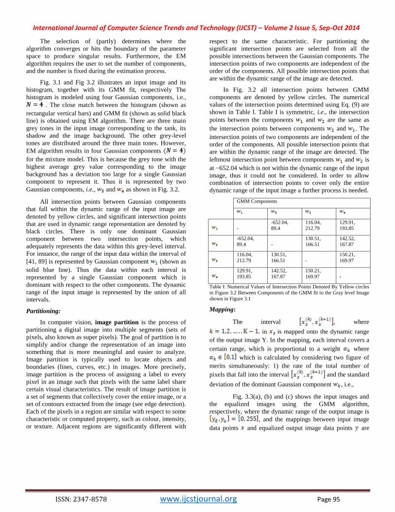
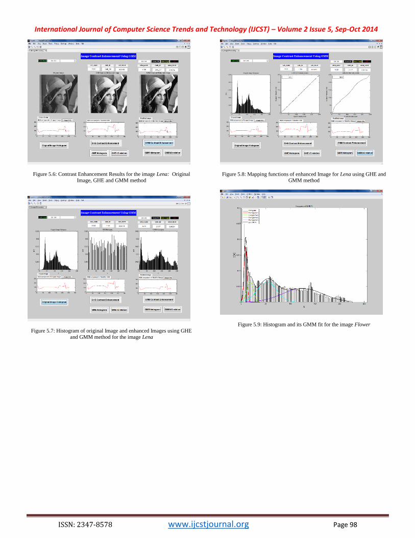
Figure 5.6: Contrast Enhancement Results for the image Lena: Original

Image, GHE and GMM method

Figure 5.7: Histogram of original Image and enhanced Images using GHE

and GMM method for the image Lena

Figure 5.8: Mapping functions of enhanced Image for Lena using GHE and GMM method

Figure 5.9: Histogram and its GMM fit for the image Flower




Figure 5.10: Histogram of original Image and enhanced Images using GHE

and GMM method for the image Flower

Figure 5.11: Histogram and its GMM fit for the image Pepper

Figure 5.12: Histogram of original Image and enhanced Images using GHE and GMM method for the image Pepper

Figure 5.13: Mapping functions of enhanced Image for Pepper using GHE

and GMM method

V. CONCLUSION

Image Contrast Enhancement using Gaussian

Mixture Modelling (GMM) has been Implemented and

analyzed mathematically. A performance comparison with

state-of-the-art techniques like GHE shows that the

implemented algorithm gives good results in terms of

AMBE, DE and EBCM. The comparison table has given

below

Image Contrast Enhancement Comparisons for GHE &

GMM

AMBE DE EBCM

Sl

.

No.

Image

Name GHE

GM

M GHE

GM

M GHE GMM

1

Woman

darkhair 20.12 4.599 1.747 2.147 0.01868 0.0404

2 Lena 31.88 14.29 1.791 2.137 0.03418 0.08234

3 Flower 51.62 17.23 1.791 2.239 0.02978 0.03708

4 Tower 12.7 2.046 1.791 2.277 0.103 0.135

5 Pepper 7.041 0.932 1.797 2.239 0.03592 0.05909

AMBE means Absolute Mean Bit Error, a lower value

indicates the better brightness preservation.

DE means Discrete Entropy, a higher value indicates an

image with richer details.




EBCM means Edge Based Contrast Measure, a higher value

indicates the contrast is improved

REFERENCES

[1] Turgay Celik and Tardi Tjahjadi,”Automatic Image

Equalization and Contrast Enhancement Using Gaussian

Mixture Modeling”, IEEE Transactions On Image

Processing, Vol. 21, No. 1, January 2012.

[2] R. C. Gonzalez and R. E. Woods, Digital Image

Processing, 3rd ed. Upper Saddle River, NJ, USA:

Prentice-Hall, Inc., 2006.

[3] D. Jobson, Z. Rahman, and G. Woodell, “A multiscale

retinex for bridging the gap between color images and

the human observation of scenes,” IEEE Trans. Image

Process., vol. 6, no. 7, pp. 965–976, Jul 1997.

[4] J. Mukherjee and S. Mitra, “Enhancement of color

images by scaling the dct coefficients,” IEEE Trans.

Image Process., vol. 17, no.10, pp. 1783–1794,Oct 2008.

[5] S. Agaian, B. Silver, and K. Panetta, “Transform

coefficient histogram-based image enhancement

algorithms using contrast entropy,” IEEE Trans. Image

Process., vol. 16, no. 3, pp. 741–758, Mar 2007.

[6] R. Dale-Jones and T. Tjahjadi, “A study and

modification of the local histogram equalization

algorithm,” Pattern Recognit., vol. 26, no. 9, pp. 1373–

1381, September 1993.

[7] T. K. Kim, J. K. Paik, and B. S. Kang, “Contrast

enhancement system using spatially adaptive histogram

equalization with temporal filtering,” IEEE Trans.

Consumer Electron., vol. 44, no. 1, pp. 82–87, Feb 1998.

[8] C.-C. Sun, S.-J. Ruan, M.-C. Shie, and T.-W. Pai,

“Dynamic contrast enhancement based on histogram

specification,” IEEE Trans. Consumer Electron., vol. 51,

no. 4, pp. 1300–1305, Nov 2005.

[9] Y.-T. Kim, “Contrast enhancement using brightness

preserving bi-histogram equalization,” IEEE Trans.

Consumer Electron., vol. 43, no. 1, pp. 1–8, Feb 1997.

[10] Y. Wang, Q. Chen, and B. Zhang, “Image enhancement

based on equal area dualistic sub-image histogram

equalization method,” IEEE Trans. Consumer Electron.,

vol. 45, no. 1, pp. 68–75, Feb 1999.

[11] S.-D. Chen and A. Ramli, “Minimum mean brightness

error bi-histogram equalization in contrast

enhancement,” IEEE Trans. Consumer Electron., vol.49,

no.4, pp. 1310–1319, Nov 2003.

[12] S.-D. Chen and A. Ramli, “Contrast enhancement using

recursive mean- separate histogram equalization for

scalable brightness preservation,” IEEETrans. Consumer

Electron.,vol. 49, no. 4, pp. 1301–1309, Nov 2003.

[13] M. Abdullah-Al-Wadud, M. Kabir, M. Dewan, and O.

Chae, “A Dynamic Histogram Equalization for Image

Contrast Enhancement,” IEEE Trans. Consumer

Electron., vol. 53, no. 2, pp. 593–600, May 2007.

[14] C. Wang and Z. Ye, “Brightness preserving histogram

equalization with maximum entropy: a variational

perspective,” IEEE Trans.Consumer Electron.,vol. 51,

no. 4, Nov 2005.

[15] C. Wang, J. Peng, and Z. Ye, “Flattest histogram

specification with accurate brightness preservation,” IET

Image Process., vol.2, no. 5, pp. 249–262, Oct 2008.

[16] T. Arici, S. Dikbas, and Y. Altunbasak, “A Histogram

Modification Framework and Its Application for Image

Contrast Enhancement,” IEEE Trans. Image Process.,

vol. 18, no. 9, pp. 1921–1935, Sep 2009.

[17] S. Hashemi, S. Kiani, N. Noroozi, and M. E.

Moghaddam, “An image contrast enhancement method

based on genetic algorithm,” Pattern Recognit. Lett.,

vol.31, no. 13, pp. 1816–1824, 2010.

[18] D. Reynolds and R. Rose, “Robust text-independent

speaker identification using gaussian mixture speaker

models,” IEEE Trans. Speech Audio Process., vol. 3,no.

1, pp. 72–83, Jan 1995.

[19] R. O. Duda, P. E. Hart, and D. G. Stork, Pattern

Classification, 2nd ed. Wiley-Interscience, Nov 2000.

[20] M. Figueiredo and A. Jain, “Unsupervised learning of

finite mixture models,” IEEE Trans. Pattern Anal. Mach.

Intell., vol. 24, no. 3, pp. 381–396, Mar 2002.

[21] M. Abramowitz and I. A. Stegun, Handbook of

Mathematical Functions with Formulas, Graphs, and

Mathematical Tables. New York: Dover Publications,

1965.


Documents

Comparison of Automatic Image Contrast … of Automatic Image Contrast Enhancement Using ... of an input image or wavelet transform of an input image. ... uses a small window that