Comparison of a linear and a nonlinear washout for motion

J IIIILJLI... 111111111111111

NASA TECHN ICA L NOTE ^|BB^P\ NASA TN D-8157

00 """^S sca LOAN COPY: RET^B ^^ AFWL TECHNICAL 5S S y

K1RTLAND AFB, Sa?| * ^

COMPARISON OF A LINEAR AND A NONLINEARWASHOUT FOR MOTION SIMULATORS UTILIZINGOBJECTIVE AND SUBJECTIVE DATA FROMCTOL TRANSPORT LANDING APPROACHES

/<’^ r^,Russell V. Parrish and Dennis J. Martin, Jr. \

’3

Lanpley Research Center \\ 4’oamo^,

Hampton, Va. 23665 \ <1<2?~&1^-le-i6^

NATIONAL AERONAUTICS AND SPACE ADMINISTRATION WASHINGTON, D. C. JUNE 1976

https://ntrs.nasa.gov/search.jsp?R=19760019106 2018-04-10T14:20:42+00:00Z

TECH LIBRARY KAFB, NM

0133150

1. Report No. 2. Government Accession No. 3. Recipient’s Catalog No.

NASA TN D-81574. Title and Subtitle 5. Report Date

COMPARISON OF A LINEAR AND A NONLINEAR WASHOUT FOR June 1976MOTION SIMULATORS UTILIZING OBJECTIVE AND SUBJEC- 6. Performing Organization Code

TIVE DATA FROM CTOL TRANSPORT LANDING APPROACHES7. Author(s) 8. Performing Organization Report No,

Russell V. Parrish and Dennis J. Martin, Jr. L-10593

10. Work Unit No.

9. Performing Organization Name and Address ^04 OQ 41 01

NASA Langley Research Center ,, contract Grant No---------Hampton, Va. 23665

13. Type of Report and Period Covered

12. Sponsoring Agency Name and Address Technical NoteNational Aeronautics and Space Administration ,4 Sponsoring Agency Code’Washington, D.C. 20546

15. Supplementary Notes

Dennis J. Martin, Jr.: Electronic Associates, Inc., Hampton, Va.

16. Abstract

Objective and subjective data gathered in the process of comparing a linear and a non-

linear washout for motion simulators reveal that there is no difference in the pilot-performance

measurements used during instrument-landing-system (ILS) approaches with a Boeing 737

conventional take-off and landing (CTOL) airplane between fixed-base, linear-washout, and

nonlinear-washout operations. However, the subjective opinions of the pilots reveal an

important advance in motion-cue presentation. The advance is not in the increased cue

available over a linear filter for the same amount of motion base travel but rather in the

elimination of false rotational rate cues presented by linear filters.

17. Key Words (Suggested by Author(s)) 18. Distribution Statement

Landing approach Unclassified Unlimited

Washout systemCoordinated washout

Motion-cue evaluation Subject Category 05

19. Security Classif. (of this report! 20. Security Classif. (of this page) 21. No. of Pages 22. Price’

Unclassified Unclassified 81 $4.75

For sale by the National Technical Information Service. Springfield, Virginia 22161

r

COMPAMSON OF A LINEAR AND A NONLINEAR WASHOUT

FOR MOTION SIMULATORS UTILIZING OBJECTIVE AND SUBJECTIVE DATA

FROM CTOL TRANSPORT LANDING APPROACHES

Russell V. Parrish and Dennis J. Martin, Jr.*Langley Research Center

SUMMARY

Objective and subjective data gathered in the process of comparing a linear and anonlinear washout for motion simulators reveal that there is no difference in the pilot-

performance measurements used during instrument-landing-system (ILS) approaches with

a Boeing 737 conventional take-off and landing (CTOL) airplane between fixed-base,linear-washout, and nonlinear-washout operations. However, the subjective opinions of

the pilots reveal an important advance in motion-cue presentation. The advance is notin the increased cue available over a linear filter for the same amount of motion basetravel but rather in the elimination of false rotational rate cues presented by linear filters.

INTRODUCTION

Two methods of providing motion cues to a moving-base six-degree-of-freedomairplane simulation are currently available at the Langley Research Center. A linear

method, essentially Schmidt and Conrad’s coordinated washout (refs. 1 and 2), is docu-mented in reference 3; and a nonlinear method, coordinated adaptive washout, is docu-mented in references 4 and 5.

A comparison of the two methods has been made in which each method was appliedto a Boeing 737 conventional take-off and landing (CTOL) airplane by using the Langleyvisual-motion simulator (refs. 6 and 7). The evaluation process consisted of the collec-tion of objective and subjective data from 135 simulated instrument-landing-system (ILS)approaches, as well as subjective data from standard maneuvering about straight-and-level flight for specific motion-cue evaluation.

This paper will present both the objective and subjective results of this study,although the intended emphasis is on the subjective results, which indicate a significantadvance in motion-cue presentation. The significant advancement is not in the increased

*Electronic Associates, Inc., Hampton, Va.

cue available over a linear filter for the same amount of motion-base travel (ref. 5) but

rather in the elimination of false rotational cues presented by linear filters.

SYMBOLS

Measurements and calculations were made in U.S. Customary Units. They are

presented herein in the International System of Units (SI) with the equivalent values given

parenthetically in the U.S. Customary Units,

A,B,C main effects in analysis of variance

-iAB,AC,BC two factor interactions in analysis of variance

ABC three factor interaction in analysis of variance

Ai ,A,,A, acceleration lead parameters for translational channel lag compensation,1

sec"

ai ,ao,a3 damping parameters for second-order translational washout filters, rad/sec

Bi,Bo,B3 velocity lead parameters for translational channel lag compensation, sec

bi,b2,b3 frequency parameters for second-order translational washout filters, rad/sec2

4bx,by coefficients for position penalties in cost functions, per sec*

o

b,^ coefficient for yaw-position penalty in cost function, per sec

Ci,Cq,Co translational acceleration braking parameters, per sec

’C mean aerodynamic chord, m (ft)

2Cy,Cy coefficients for velocity penalties in cost functions, per sec"

DPR scale factor, deg/rad

dy,d,. damping parameters for second-order translational washouts, per sec

o

Qv,e-v frequency parameters for second-order translational washouts, per sec

22

eî, parameter for first-order yaw washout, per sec

^c x^c v body-axis longitudinal and lateral accelerations at centroid location after

low-pass filtering, m/sec (ft/sec-)

fg ^ body-axis vertical acceleration (referenced about Ig) at centroid location

after high-pass filtering, m/sec2 (ft/sec-)

î x’î v’î z inertial-axis translational acceleration commands prior to translational

washout, m/sec2 (ft/sec-)

fj^x’^ v inertial-axis specific-force error signals, m/sec- (ft/sec")

^1 x’î v’î z components in inertial axis of filtered body-axis vertical acceleration

at centroid location, m/sec (ft/sec )

f^ artificial yaw-error signal, m/sec^ (ft/sec^)

^s-x^s v body-axis longitudinal and lateral acceleration at centroid location,m/sec^ (ft/sec^)

fg ^body-axis vertical acceleration (referenced about Ig) at centroid location,m/sec2 (ft/sec2)

fx,fy,fz airplane body-axis translational accelerations, m/sec2 (ft/sec2)

f^ g body-axis vertical acceleration at centroid location, m/sec2 (ft/sec2)

Gi glide-slope error gain

g gravitational constant, m/sec2 (ft/sec2)

h altitude, m (ft)

hg commanded altitude, m (ft)

hy height of airplane center of gravity at touchdown, m (ft)

KQ heading error gain

3

1

Ki gain parameter of roll flight-director filter

Ko damping parameter of roll flight-director filter, deg/sec

Ko frequency parameter of roll flight-director filter, deg/sec

v ’K ’K \c,l> c,2’ c,3\ coefficients for initial-condition penalties in cost functions, per sec

^,4^0,5 J^l^M ga^n parameters, sec3/2 (sec3/ft2)^,3^,3;

^ 2’^ 2 Sai11 parameters, sec6/4 (sec6/^4)

Ky yaw-damper gain

KQ yaw-damper parameter, per sec

0

Kî, yaw gain parameter, sec-

kp,kQ,kr scaling parameters for angular rates

kr> T 1 ,kr, T 1 ,^-r 1 parameters of signal-shaping network, per m (per ft)P;1 ?1’ ’if1)1-’ ’f-

k^, T 9,kn T 9,kT. 9 parameters of signal-shaping network, secf)’)" 4?-1-?-’ 5"

^v T 3^0 T S^r 3 parameters of signal-shaping network, per sec

k 1 k o gain parameters of vertical channel high-pass filterz,r z,^

kn ,kn q gain parameters of longitudinal channel low-pass filter

^ch 1 ^(b 2 Sai" parameters of lateral channel low-pass filter

^ I^-Q i^l lead parameters for rotational channel lag compensation, sec

fsgn (A,B) when |A| > Ba?(A,B) operator equal to

\A when |A| s B

4

ll

Ly localizer error rate limit, deg/sec

L^) flight-director roll limit, deg/sec

p,q,r body-axis angular velocity commands, rad/sec

p’,q’,r’ body-axis angular tilt velocity, rad/sec

p",q",r" scaled body-axis aircraft angular velocities, rad/sec

p ,q ,r body-axis aircraft angular velocities, rad/sec

P.- i P., oÂ,J. A,O adaptive parameters, position limited

w^jp ?,p ., adaptive parameters, position limited, sec/m (sec/ft)

Px,l’Py,l\_i 7 adaptive parameters, rate limited^S’Py.Sjp’ n,p’ adaptive parameters, rate limited, sec/m (sec/ft)^9" y"

FX 1’^ 1 >̂ adaptive-parameter rates, per sec

^’"y.sj

P" qiP" o adaptive-parameter rates, per m (per ft)x?" y"

? ,(o),p’_ <(o)^y’

/ initial conditions on adaptive parameters, rate limited

Px,3()’Py,3()JPX 2^’^v 2^ initial conditions on adaptive parameters, rate limited, sec/m (sec/ft)

p, adaptive yaw parameter, position limited

p’ adaptive yaw parameter, rate limited

p" adaptive-yaw-parameter rate, per sec

5

p* (o) initial condition on adaptive yaw parameter, rate limited

R range from runway, m (ft)

RX,RV,RZ centroid location with respect to center of gravity, m (ft)

Si pitch input to pitch flight director, deg

Sq output of first-order pitch input lag, deg

Sx,Sv scale factors on fg ^,ig y

s Laplace operator

t time, sec

t^ starting time for roll flight-director operation

At time step size, sec

Vn velocity limit, m/sec (ft/sec)

Wx,Wy angular-rate weighting coefficient, m2/sec2 (ft2/sec2)

x,y,z commanded inertial translational position of motion simulator, m (ft)

x,y,z commanded translational positions after compensation, m (ft)

x,. p,y, p,,Zy T,. scale factors on position limits

^b’yb’^b intermediate inertial-axis translational acceleration commands,m/sec2 (ft/sec2)

^’yd?2^ inertial-axis translational position commands, m (ft)

x,,y,,z, inertial-axis position limits for translational channels, m (ft)

x Earth-axis longitudinal coordinate of airplane center of gravity, m (ft)

XQ longitudinal coordinate of runway touchdown point, m (ft)

6

Xp,yp,Zp coordinates of pilot’s station with respect to center of gravity in body-axis system, m (ft)

Xp (;,yp c?2? c coordinates of centroid location with respect to pilot’s station in body-axis system, m (ft)

x^. x-distance of airplane center of gravity from runway, m (ft)

y^ distance behind runway touchdown point of localizer-beam origin, m (ft)

y Earth-axis lateral coordinate of airplane center of gravity, m (ft)

YQ lateral coordinate of runway touchdown point, m (ft)

y-, y-distance of airplane center of gravity from runway, m (ft)

YnVo yaw-damper states

êut actuator extension for selected neutral point, m (ft)

fS sideslip angle, rad

y- commanded glide-slope angle, deg

6 a aileron-deflection angle, rad

fig elevator-deflection angle, rad

fiy rudder-deflection angle, rad

^R v yaw-damper contribution to rudder command, rad

firp throttle position, deg

e, vertical glide-slope error, m (ft)

ey localizer error, deg

e-y jg rate-limited localizer error, deg

7

7 localizer-error lag, cleg

Cy glide-slope error, deg

ci, heading error, deg

&i, i scaled heading error, deg

0^ actual airplane pitch angle, deg

OQ commanded pitch angle, deg

0g pitch-command signal, deg

^^ 1 damping parameter for vertical channel high-pass filter

L,?^) damping parameters of low-pass filters

T yaw-damper parameter

(f) actual airplane roll angle, deg

(^g commanded roll angle, deg

(f)f roll flight director filter input, deg

(f>. intermediate roll-command angle, deg

(b roll-command signal, deg

0-p^-p^l variables of roll flight-director filter, deg

i^ ,6,(j) commanded inertial angular position of motion simulator, rad

\^,8,(p commanded angular positions after compensation, rad

i// actual airplane heading, deg

â’â’â airplane angular velocities, rad/sec

8

i^_ commanded heading, deg

^T’^T’^T commanded inertia! tilt rates, rad/sec

^n z 1 frequency parameter of vertical channel high-pass filter, rad/sec

"n 9’^n (b frequency parameters of low-pass filters, rad/sec

Subscript:

meas measurement by instrument mounted on motion simulator

A dot over a variable indicates the time derivative of that variable.

THE FUNDAMENTAL DIFFERENCE

Figure 1 illustrates the fundamental difference in terms of motion cues between a

linear filter and a nonlinear adaptive filter for the first-order filter case. The difference

is anomalous rate cue presented by the linear filter as the pulse input in rate returns tozero. This false cue is most evident for pulse-type inputs and disappears as the input

becomes sinusoidal. Thus, the fundamental difference between the linear and nonlinear

filters varies dependent upon the responsiveness of the vehicle and the pilot’s input in

each axis, but not upon the parameter values of the linear filter.

Figure 2 presents a comparison of the linear and nonlinear washouts as applied toa simulation of a Boeing 737 conventional take-off and landing (CTOL) airplane for an

aileron pulse input. Washout responses for typical pilot inputs in all axes will be pre-sented later. As shown in figure 2, the linear washout represents the roll acceleration

well (ignoring the scaling), while presenting the false cue in rotational rate. The non-

linear washout practically ignores the acceleration reversal (Time 8 seconds) in order

to eliminate the false rate cue. The importance of presenting the rotational rate cue

properly rather than the rotational acceleration cue will be demonstrated in the compar-ison of the two washouts for roll inputs.

THE WASHOUT CIRCUITRY

The adapted version of Schmidt and Conrad’s linear-coordinated washout circuitryused in this study is shown in figure 3 in block-diagram form. The detailed equationsare presented in appendix A. The function of the circuitry is to represent the transla-

tional accelerations and the rotational rates of the simulated airplane while constraining

9

the motion commands to be within the hardware capabilities. The concept of this coordi-

nated washout circuitry is to represent longitudinal and lateral translational cues by uti-

lizing both translational and rotational motions and to obtain rotational washout through

elimination of the false gravitational g cues that would be induced by a rotational

movement.

The selection of the parameters for the washout circuitry began with employment

of the values suggested in figure A.7 of reference 2. A representative "worst case"

instrument-landing-system (ILS) approach was made with the fixed-base simulator, and

the resulting translational accelerations and rotational rates were placed on tape. The

tape was then used iteratively to drive the motion software for parameter variation.

Initial modification of the parameters was made to constrain the motions to remain

within the motion limits of the hardware. Further modification of the parameters to

improve the fidelity of the motion cues, in terms of time-history comparisons of airplane

motion cues (simulated flight data) plotted against washout commands to represent these

cues, was then made.

Final determination of the linear-washout parameters was then made based on the

subjective opinions of three participating research pilots, and these parameter values

are presented in table I. The major emphasis of this portion of the parameter-selection

process fell on the roll channel parameters and is discussed in reference 8. The impor-

tance of the roll motion in the overall simulation is to be elaborated on later.

The nonlinear-washout method used in this study, coordinated adaptive washout,

is shown in figure 4 in block-diagram form. The detailed equations are presented in

appendix B. The concept of the nonlinear washout is similar to that of the linear cir-

cuitry, with the major differences being that the washout is carried out in the inertial

reference frame rather than in the body-axis system, and employs nonlinear adaptive

filters rather than the linear filters.

Parameter selection for the nonlinear circuitry began with selection of a set to

constrain the "worst case" ILS approach motions to remain within the hardware capa-

bilities. Modification was then made to improve the fidelity of the cues in terms of

time-history comparisons, and final modification based on subjective opinions of three

participating pilots concluded the process. The parameter values selected are presented

in table n.

It should be emphasized that the parameters presented for each washout were

chosen for a particular airplane simulation and a particular motion base by the three

participating pilots. These parameters would perhaps vary with a change in airplane,

task, motion base, or even with a change in pilots. However, the values are presented

10

here as the results of an attempt to optimize subjectively for the stipulated simulation.

Since the nonlinear washout acts adaptively on the airplane motions to constrain the base

excursions, it intuitively follows, and recent experience has indicated, that changes in

airplane, tasks, or pilots, which determine the inputs to the washout, do not necessarily

imply changes in washout parameters for satisfactory performance to be maintained with

the nonlinear washout. It is anticipated, however, that a change in motion-base charac-

teristics would require changes in the parameters of the washout in order to achieve the

optimal performance.

COMPARISON OF THE TWO WASHOUT CIRCUITMES

The method of comparing the two washout circuitries was originally intended to

consist of an analysis of variance based on objective-data results and also a comparison

of subjective opinions. However, upon implementation of the linear washout, an analysis

of variance was carried out comparing fixed-base operation against linear-washout

operation. The results of this comparison are presented in reference 8, and the analysis

of variance is included in a later section herein. Upon implementation of the nonlinear

washout some time later, the objective-data base was extended to include nonlinear

washout operation, and a new analysis of variance was conducted.

Additionally, between the times of implementation of the two circuitries, a major

change in the lateral handling characteristics of the Boeing 737 airplane simulator was

made. The change arose as a result of a comparison of newly acquired flight data with

simulated flight data and involved the addition of a f3 feedback term in the simulation

equations of the yaw damper. Appendix C contains the equations of the yaw damper, both

with and without the ft feedback term.

Figure 5 presents the unmodified (without ft feedback) 737 simulator response to

the aileron pulse input of figure 2, along with the linear- and nonlinear-washout responses

to the airplane motions. The responses of figure 2 are those of the modified simulator

(with ft feedback). The major result of the modification in terms of handling charac-

teristics was that rolling to a desired bank angle became a much simpler task, as evi-

denced by a comparison of the roll rates presented in figures 2(a) and 5(a).

Since the objective data for the fixed-base and linear-washout operations had been

obtained from the simulator without the ft feedback term, the comparison data for

nonlinear operations were also collected in this mode. Subjective data were solicited both

without and with the ft feedback term in the yaw-damper equations and are presented in

a later section under these classifications.

11

TASK CONDITIONS AND DATA BASE

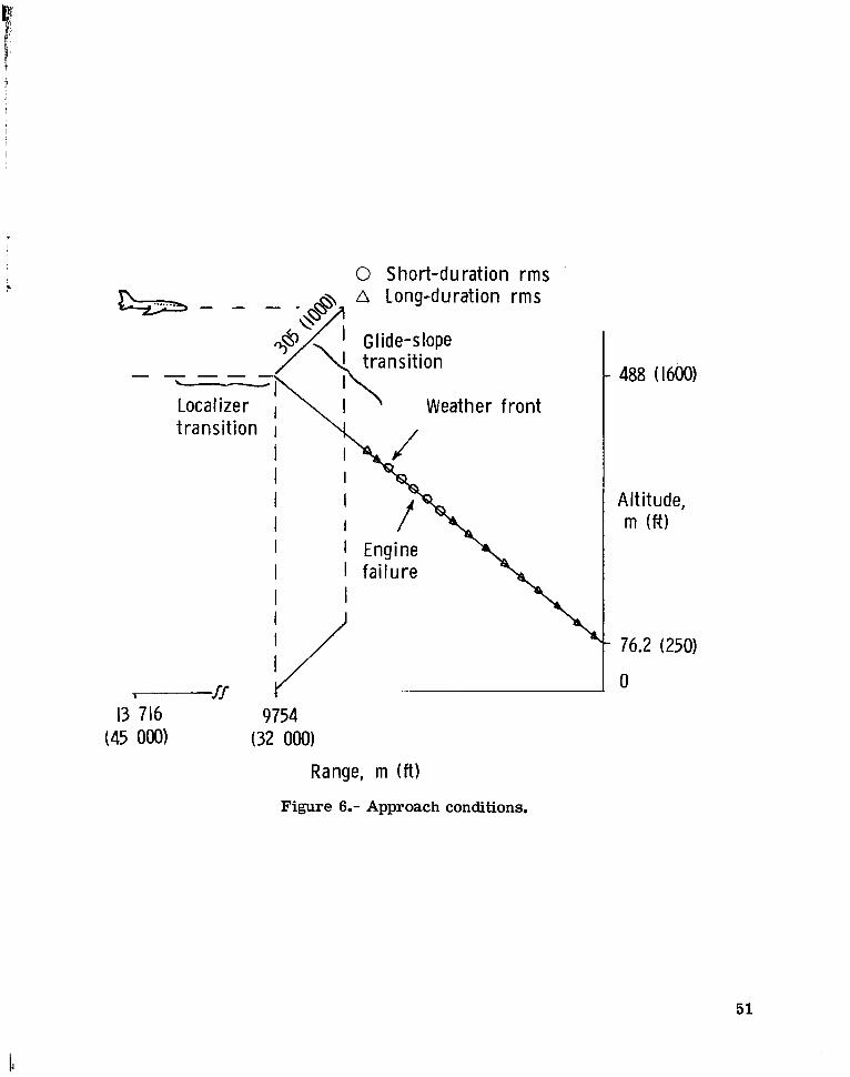
Figure 6 illustrates the ILS task, which consisted of the following: (1) a transition

to the localizer beam, followed by (2) a transition to the glide slope, and (3) the ensuing

approach down to about 76 m (250 ft). Three approach conditions were provided: the

standard approach previously described, the standard approach with instantaneous

encounter of a weather front (a 10 knot crosswind with moderate turbulence), and the

standard approach with the occurrence of an engine failure. Instrumentation consisted

of an attitude-direction indicator, vertical-speed indicator, a horizontal-situation indi-

cator, altimeter, airspeed indicator (both calibrated and true), meters for angles of

attack and sideslip, and a turn and bank indicator.

The approach conditions were flown under fixed-base conditions and under two

moving-base conditions. Motion was restricted to five degrees of freedom because:

(1) extreme hydraulic noise is induced by the heave motion of the synergistic base (all six

actuators have to move alike to present a heave cue), and (2) only a small amount of verti-

cal cue was available.

The small amount of vertical cue available is due to a combination of the position

limits of the motion base and the short-period frequency of the 737 airplane in the landing-

approach configuration. Since the position limits of the synergistic motion base change

as the orientation of the base varies, the position limits used in determining the linear

washout parameters must be conservative. For the motions involved in this study, the

vertical-position limits were chosen to be 0.457 m (1.5 ft). The low-frequency content

of the normal acceleration of the airplane (less than 1 rad/sec, neglecting turbulence) is

due to the low short-period frequency. (See table III.) The amount of vertical cue avail-

able for motion simulation is thus less than 0.05g (the product of amplitude and frequency

squared). The participating pilots felt that the vertical cue available was not worth the

noise distraction.

During the performance of the landing-approach task under the aforementioned con-

ditions, root-mean-square (rms) data were collected over two regimes. A short-duration

regime, intended to reflect the immediate effect of the weather front and the engine-failure

conditions, and a longer duration regime, intended to evaluate total performance, were

used. The regimes overlapped and were based on airplane range. (See fig. 6.) The rms

values were obtained for glide-slope deviation, localizer deviation, pitch-command bar

deviation, roll-command bar deviation, and speed-command bar deviation. The equations

for the flight director used in this study are presented in appendix D.

Subjective data consisted of pilot comments solicited during objective-data collection

from the three participating pilots, as well as subjective evaluation data from standard

maneuvers about straight-and-level flights by seven pilots.

12

I

OBJECTIVE-DATA RESULTS

The objective-data results are presented in the form of two analyses of variance

experiments: the first comparing fixed-base operation against linear-washout operation,

and the second comparing fixed-base, linear-washout, and nonlinear-washout operations.

Both experiments utilized the simulated 737 airplane without the ft feedback term in the

yaw damper.

Comparison of Fixed-Base Operation With Linear-Washout Operation

The design of this experiment consisted of the 2 x 3 x 3 factorial design (ref. 9)

shown in table IV. The fixed-effect factors involved are pilots, approach conditions, and

linear motion against fixed-base operation. The results of the analyses of variance of

the 10 separate rms measurements are shown in table V. Significance of the one-tailed

F-tests is indicated by a single asterisk for the 5-percent level and by a double asterisk

for the 1-percent level.

The results indicate significant differences in mean rms performances between

pilots and also between approaches. No significant differences in mean rms performances

are found between motion and fixed-base operation. The occasional significance of the

two-factor interaction AC indicates that the differences between pilots varied with the

approach condition over all motion conditions, or, alternately, the differences in per-

formance between approaches varied from pilot to pilot, regardless of the motion condi-

tion, for some of the performance measures.

Comparison of Fixed-Base, Linear-Washout, and

Nonlinear-Washout Operations

After implementation and parameter selection were completed for the nonlinear wash-

out, the ILS task was repeated to expand the objective-data base to include the nonlinear

washout. The expanded experiment consisted of the 3 x 3 x 3 factorial design shown in

table VI. The results of the 10 new analyses of variance of the rms measurements are

shown in table VII. Significance of the one-tailed F-tests is indicated by a single asterisk

for the 5-percent level and by a double asterisk for the 1-percent level. Again, the

results indicate significant differences between pilots and approaches, and significance

of the two-factor interaction AC, as shown in table V.

The now-occasional significance between motion conditions is not frequent enough to

warrant any claims of differences, particularly in light of the possibility of heterogeneity

of data. (The nonlinear data were collected separately and at a later date.) This con-

clusion can also be drawn concerning the significance of the interactions involving

motion B.

13

Further, the occasional significances between motion conditions are not consistent

across the performance measures. It might be expected that the significant differences

indicated for the localizer measurements would be reflected also in the roll-command bar

measurements. Likewise, significance of the pitch bar measurements for long durations

might be expected to be accompanied by glide-slope and speed-measurement differences,

and perhaps by the short-duration complement measurements also.

SUBJECTIVE-DATA RESULTS

Pilot comments obtained during this study fell purposefully into two categories:

general comments from three pilots on the effectiveness of motion, and specific comments

from seven pilots on the representation of motion cues for standard maneuvers by each

washout method.

General Comments

The three pilots participating in the objective-data task shared the opinion that

motion greatly increased the realism of the simulation and also increased the pilot work-

load. All three pilots preferred the nonlinear washout to the linear washout, although they

preferred the linear washout to fixed-base operation.

Specific Comments

Seven pilots participated in a subjective evaluation of the linear- and nonlinear-

washout methods by rating the motion cues presented by each method for throttle, column,

wheel, and pedal inputs about a straight-and-level condition in a landing-approach mode.

Each pilot determined his own evaluation inputs and also flew portions of the ILS landing

approach. In addition to rating the motion for each type of control input, the pilots were

asked to rate how well the overall motion came to representing that of an airplane (e.g.,

does it "feel" like an airplane). The initial rating categories were excellent, good, fair,

poor, and unacceptable, but the pilots rather consistently used ratings halfway between

two of the given categories.

The lateral ratings and the overall motion ratings were obtained for both of the

lateral-handling characteristic cases: without the fS feedback in the yaw damper, and

with the (3 feedback in the yaw damper. The longitudinal-handling characteristics were

not affected by this change. The subjective results of this evaluation with the f3 feed-

back in the yaw damper are also presented in reference 10.

Longitudinal inputs.- The results of the evaluations involving longitudinal inputs are

presented in table VIII, with an open symbol representing the rating of the linear method

14

and a solid symbol representing the nonlinear-method rating. The first four pilots,

represented by the triangular symbols, have had actual 737 cockpit experience.

Throttle inputs: Figure 7 presents typical time histories for a change in throttle

setting. Inputs to the washouts from the simulated airplane, if ignoring the body-inertial

transformations, are the longitudinal acceleration (scaled at one-half) fg x an^ thG pitch

rate q_. As figure 7 shows, very little difference exists between the linear and nonlinearcL

responses for these inputs. The fundamental difference between the two pitch-rate filters

is obscured in order to represent the decrease in fg ^ a time equal to 6 seconds.

The pilot ratings for throttle changes, as shown in table Vin, are the same for each

method. (No change in a pilot’s rating between linear and nonlinear washout is indicated

by the open symbol appearing above the solid symbol.) Indeed, when given the methods

back to back for throttle comparison, the pilots could not detect that a change had been

made.

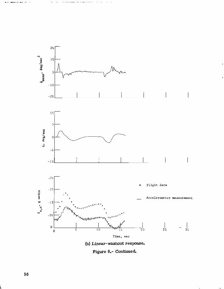
Column inputs: Time histories of an elevator doublet input are presented in fig-

ure 8. As with throttle inputs, the fundamental difference between the pitch-rate filters

is obscured because of the coordination of pitch with longitudinal acceleration. The non-

linear response does contain more pitch rate and more pitch-angle change, resulting in

better phasing of the fg,x cue. However, the differences are small, and four pilots rated

the washout methods the same for this control (table VIII), whereas the other three rated

the nonlinear method slightly higher.

Lateral inputs without g feedback.- The results of the evaluations of the lateral

inputs for the airplane without /3 feedback are presented in the previous format (oftable VIII) in table IX.

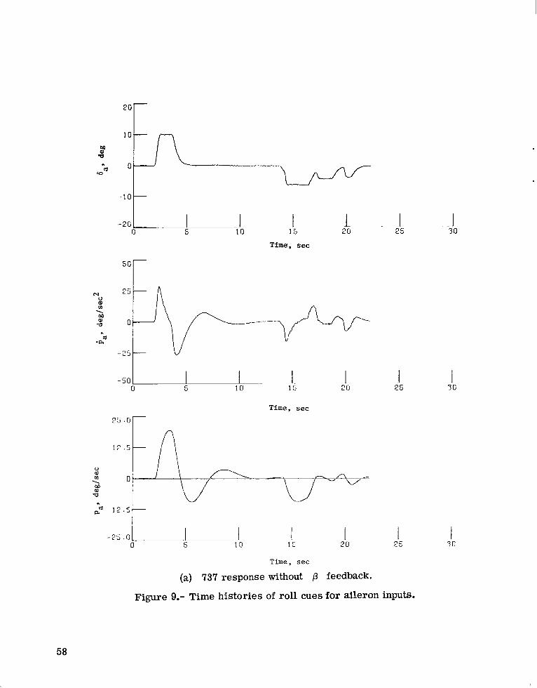
Wheel inputs: The pilots preferred to break the motion cues that accompany aileron

inputs into roll cues and yaw cues for the purpose of individual cue evaluation. Figure 9

presents time histories for the roll cues by using ailerons to bank the airplane 20 for a

30 heading change with a return to a straight-and-level condition. Without ^ feedback

in the yaw damper, the roll rate of the airplane is oscillatory, with the peak at 6 seconds

being about one-half of the peak at 3 seconds. The linear-washout response for this

case yields a second peak of p that is larger than the first peak and could give the pilot

the impression of a net left bank, rather than a right bank. This anomalous rate cue is

not present in the nonlinear-washout response.

All pilots rated the nonlinear roll cues to be at least one category higher (better)than the linear cues, and two pilot ratings are three categories higher. The poor side-

force representation by both washouts, due to lack of sufficient y-travel of the base both

to offset the misalinement of the gravity vector (due to the roll cue) and to present the

side-force cue (refs. 4 and 8), was not noticed by any of the pilots.

15

?

Figure 10 presents the time histories of the yaw cues for the previous maneuver.

At a time of 18 seconds, when the yaw rate of the airplane returns to zero, the linear

washout presents an anomalous rate cue. The nonlinear response does not contain this

anomalous cue. Three of the pilots rated the yaw cues of each washout to be approxi-

mately the same; one of these three gave each washout a rating of good, and the other two

rated the nonlinear washout one-half category higher than the linear washout. The four

other pilots rated the nonlinear washout somewhat higher than the linear washout, with

one change of one category, and three changes of two categories.

Pedal inputs: Since little pedal control is used on the 737 airplane, the pilot ratings

for roll and yaw cues are based mostly on wheel inputs. However, all the pilots conducted

rudder maneuvers for each washout; no resulting changes were made in the roll and yaw

ratings. The yaw time histories for a typical rudder input are shown in figure 11, and

figure 12 presents the roll time histories for the same inputs.

Overall airplane feel: All seven pilots rated the nonlinear washout to be at least

one category higher than the linear washout in terms of overall airplane feel.

Lateral inputs with f3 feedback.- The results of the evaluations of the lateral

inputs for the simulated airplane with P feedback in the yaw damper (which more

closely approximates the flight vehicle) are presented in table X.

Wheel inputs: As with the previous case, the motion cues resulting from lateral

inputs are presented in terms of roll- and yaw-cue ratings. Figure 13 presents the roll-

cue time histories for an aileron-induced bank of 20 for a 30 heading change with a

return to straight and level. In this case, the anomalous roll rate of the linear washout

is evident, and the subjective evaluations of all seven pilots reflect the fact that this

motion was felt to be unnatural for an airplane. All pilots rated the nonlinear roll cues

to be at least != categories higher than the linear cues, and three pilot ratings were

2^ categories higher. Again, none of the pilots noticed the poor side-force representation

of both washouts.

Figure 14 presents the yaw-cue time histories for the previous aileron maneuver.

Again, the anomalous rate cue was present; the pilots particularly noticed a negative rate

when the airplane rate r^ returned to zero during maneuvers of this type. This fact is

reflected in the ratings of table X, in which the nonlinear-washout ratings are at least one

category higher, and four ratings are two higher.

Pedal inputs: No changes were made in the roll- and yaw-cue ratings as a result

of the rudder maneuvers conducted by each pilot. The yaw time histories for a typical

rudder input are shown in figure 15, and the roll time histories for the same inputs are

presented in figure 16.

16

i

Overall airplane feel: The nonlinear washout was rated by all the pilots to be at

least 1^’ categories higher than the linear washout in terms of overall airplane feel, with

each pilot noting that the roll representation had the most impact on how much the simu-

lation felt like an airplane.

CONCLUDING REMARKS

The results of this study comparing a linear-washout method with a nonlinear method

can be summarized with respect to the two types of data as follows:

Objective Data

The lack of significant differences in pilot performance for the various motion con-

ditions (fixed base, linear washout, and nonlinear washout) for the two objective experi-

ments seems to indicate that pilot performance as measured was not influenced by the

motion cues presented in this study during instrument-landing-system (ILS) approaches.

Subjective Data

The subjective results of this study, however, indicate that motion increases realism

and that the pilots prefer it to fixed-base operation. More significantly, the pilots rated

the nonlinear washout as highly preferable to the linear washout, and they specifically

objected to anomalous rotational rate cues in roll and yaw with the linear method. Since

the pilots considered roll representation to be most important in terms of the overall air-

plane feel, the elimination of the objectionable anomalous rate cues is highly desirable.

Langley Research Center

National Aeronautics and Space Administration

Hampton, Va. 23665

April 14, 1976

17

APPENDIX A

DETAILED EQUATIONS FOR THE LINEAR-WASHOUT CIRCUIT

The following is a block-by-block list of equations corresponding to figure 3:

Centroid transformation:

RX Xp + Xp^c

Ry VP + yp,c

RZ ^ + ^,0

fs,x ^ (<la + ^x + (laPa ^"y + (^Pa + ^KZ^,7 ^ + (Paâ + ^x (Pa + ^y + (â Pa)^

^^ ^ + (Pa^ â)^ + (Va - Pa)^ (P^ + ^zVariation about Ig:

^z ^,0 + S

High-pass filter:

kz,lfs,z ^l^l Tfc,z dt <z,l .f^c^ ^ dt

k^2

Low-pass filter:

Âx ^^^^ ^^x ^n^^x

^,2^^ Ây ^^n,^^ <^c,y18

I

APPENDIX A

Body to inertia! transformation, high-frequency components:

f.’ L, ^,(cos (p sin 9 cos V/ + sin 0 sin i^)1 .A. ^ f&J

fj f/. ^(coa ^ sin 0 sin ^ sin 0 cos i^)i,y -’"

^,2 fC,z(cos ^ cos 0)

Body to inertia! transformation, low-frequency components:

f* f* -(cos 9 cos ^) + f* ,,(sin 0 sin 0 cos ^ cos (p sin ip)l ,x c ,x ,y

g(cos 0 sin 6 cos i^ + sin 0 sin i^)

f*,, f* ,,(cos 6 sin i^) + f* y(sin ^ sin 0 sin ^ + cos ^ cos i//)ly c,x ^,y

g(cos ^ sin 0 sin i^ sin 0 cos \p)

Sum of low- and high-frequency components:

^x ^^ + h^

^,7 ^^y + ^,y

h^ ^.zSignal-shaping network:

^T ^.T,!^^^^ + \,T,1 J^x dt + \,T,1\,T,3 JJ^x dt dt

^T -^.T,!^^^^ ^,T,1 J^y dt ^^^^^^ jj ^y (it dt

^T kîk,^^, + kr,l 1^ (lt + ^,1^,3 JRz (it dt

Inertial to body transformation:

p’ ^(cos 6 cos ip) + 9’v(cos Q sin ip) ^,(sin 0)

19

APPENDIX A

q’ 0rp(sin (f) sin 6 cos if/ cos (j) sin i^) + ^(sin <p sin 0 sin if/ + cos 0 cos if/)

+ 4’-(sin <j) cos 9)

r’ 0rr.(cos 0 sin 0 cos ^ + sin (f) sin ^) + ^T^08 ^ sin 9 sin ^ sin ^ cos if/)

+ i^,p(cos ^ cos 0)

Scale airplane angular rates:

P" kpPa

q- kqq^

r" 14.^

Sum of airplane and tilt rates:

p p" + p’

q q" + q’

r r" + r*

Transformation to Euler rates:

(f> p + q sin 4> t3-11 Q + r cos ^ tan 6

6 q cos 0 r sin <p

i^ (q sin (f) + r cos <^>) sec 0

Angular lead compensation:

i// i// + k^^0 0 + k. ,^

y/

<? 0 + k^20

.1

APPENDIX A

Translational lead compensation;

x x^ + A^ + B^y Yd + ^d + B2yd

z ^ "’ ^’d 4’ VdTranslational washout:

"d ^x alxd blxd

^d ^y a2yd ^Yd

^d \,T. ^d b3zd

Limit prediction based on current position:

See reference 3 for equations and derivation.

21

APPENDIX B

COORDINATED ADAPTIVE WASHOUT

The following equations are those of the nonlinear washout and correspond tofigure 4. The derivation of these equations may be found in reference 5.

Longitudinal filter equations:

x PxAx ^ ^6 Pxîpc + Pxâ

^l ^l^x ^ ^^ c.x^ .^ p^Ke,!

fcl Kl > --06) F (^l - 1)px’l

/. ^ ^l ^l (-^ PX,! ^)t-0-06 (^l -0-06) [-0:1 v

^, <-0.ljPx 2 ^ 2 (fi x ^T8^- -^ + WA 0)^0- b^x -8^- c^x î-x,2 -x,2 ^ i,x ^p^ ^ x^ a ;ap^ x-ap^ x" 3?^

fr

).01 (Px,2 > ool) 0- 05 (Px 2> o05)

PX^ ^2 (-^^ Px,^ 0-01) Px,2 Px,2 (^^ Px,^ 0-05).0.01 (Px^ -0-01) [0-01 (Px^ ^-01)

P ""]

P’1 , ^ 3 fe x ^) (-ai^ -^ + WA 6)-^- b^x -ax- c^x ^^-x,3 ^,3

î,x ;^^ ^ x^ a ;^^ x ap^ x

^+ [Px,3() PX^^

22

APPENDIX B

r1 (^ > 1)

^ Px,3 (^ Px^ 1)1 (?x,3 < 1)

( 8X \ / 8x_\ Qx \9p-^ ^x ^lip^) îp-^X,l/ \ X,!/ \ X,!/

/ ax \^

^,x / ax \ , / ax \^2; px^ ^2 x^ ’^x^/_^ \ î^ ^

/ ax \ / ax \(^ Px,l ap^ âp^^) âp^gj/ 96 \_ îâp J ’i^ + Px,2 ap\ X,<i/ X,Z

/ 80 \ Qt^\^~3 ^,2 ip-- + ^\ x’^/ X)"

Y r ~l c

a^ -fg ^(sin 0 cos i^) + fg y(sin ^ cos 6 cos i^) g(cos ^ cos 0 cos i^/)x^ x,2

Qr

-g-- -fg ^(sin 6 cos i//) + fg y(sln 0 cos 6 cos ^) g(cos cj) cos 6 cos \l>)\---x,3 x,3

f. S^fg x(cos e cos 4^ + Syfg y(sin (f) sin 6 cos if/ cos <p sin i^)

g(cos 0 sin 0 cos ^/ + sin <p sin i^)

Lateral filter equations:

y py^^y ^y ^y

^ -Fy^^^y + Py,3^

23

APPENDIX B

^,1 ^ ^ ^<T cyy<T + l^*0’ ^h3y?-1 y- y?-

y

{ 0.8 ^p’ i> 0.8^

)" fp" ^> -o.o6\ \ y’1 J

Py ly’

^ I k l (-0.1 ^Py i ^ 0.8)0-06 (-y^ -0-06) [-0. v (^ < -o.j

p- ^2 (fi- <<. %) + w^ ^ b^ c-y^10.1 (Py^ ^-1) 0-01 (py,2 > ool)^,2 ^ ^, 2 (-0-1 ^y,2 - -1) Py,2 < Py,2 (-0-01 s Py^ 0-01)

:0-1 (Py^ ^0-1) I-0-01 (Py^ ^0-01)

^ -y,3 (.,y ^ ^) . W^ ^ .^ e,y^+ [Py^ Py^]^/-

S O.3 /p’ > 0.3^)"

3 (P" 3s -0.2) I y’3 /

py3 .L (,., < -o.) ^ py-3 (o s py’3 5 0-3)v y-3 J 1 (^ < 0)

/ 9y ’\ , -, /’’>y ’\ , / sy \te) ’’v y^ vte;/ y \ , ^..y , /Jl \ J y \^y,2j py’1 ^,2 "^y,2^ ^y.l)24

APPENDIX B

/ ay \ , ^yH /_iy_\ , ^ \\^j py?l ^,3 ^,3; ey^

t-^L\- -f. p -^^ f1^ ^.2 ^,2

/ 8^\ 8fi,y^j -^îâ

ftfl>y \ts v(cos ^ sin 6 sin V/ sin (f) cos i//) + g(sin (p sin 0 sin 1^ + cos cf> cos ^) -3--

^,2 }- ’y -’ ^y^

-’"^ ^s v^08 <^ sin e sln ’^ sin ^ cos ^ + 6(sln ^ sln ^ sln ^ + cos ^ cos ^/) ^^7,3 L ’y

-j opy,3

f. S-fg ,,(cos 6 sin i,i/) + Syfg y(sin <p sin 0 sin i// + cos <?> sin 8 sin )^)

g(cos <p sin 0 sin i^ sin 0 cos i^)

Yaw filter equations:

^ pâ e^

^ ^ ^ ^-^^ - [^ ^^r^ fp’; > --^

1 ^> x)

^-r ( ’ /

^ (o^ s l)I-0-4 (p^ -4) (P^ O)

\.

/8^\ /8l//\N^ ^)25

-1-

APPENDIX C

THE YAW-DAMPER EQUATIONS

The following yaw-damper equations are used in this study:

Without ^ feedback:

yi Kyr

yq -s-9 YI2 (rs -H)2 1

+4

^2 ^9.15 -^ -^7 ^.y

----2--^0-^---I -4________

0.955 ^_TS + 1

With /3 feedback:

^1 ^^ V)

fo (i^) 5 0-5)

^ [̂4 (| Sa| > 0-5)with y? and 60 y remaining as previously shown.

26

I

APPENDIX D

FLIGHT-DIRECTOR EQUATIONS

The following equations for the flight director are used in this study:

Input equations:

Xy (Xjg Xo) cos ^ + (y^ yj sin ^Yr -(x^ ^ sin ^c + (yi yo) cos ^c

R (xj + yj)

hg R tan y^ + hy

^ h êy tan"1 (^) x DPR

V"/

^ â ^c

^ ^"’ (R^) "^Pitch flight director:

fo.l4(h 50) (h < 100)

Gll^h/15 (h ^ 100)

GI limited to [o, 100]

sl -(^ + 2)

27

APPENDIX D

Si SoSo (Initial condition: So S^\

^c ^y- ÔQ limited to [-12, 12]

QS ^ + s!

Roll flight director:

t ^ s 90 t tp > 90

Ly 0.4 Ly 0.12

L0 25 L^, 15

Kg 2.8 KQ 3.8

K^ 2.833 K- 3.5714

K 2.867 Ko 3.534

K3 0.3333 Kg 0.7518

< ^^-ey^ (Initial condition: 6y ^ 0)

6y ^ limited to f-Ly, Lyi

^^ <y,jE + êy^

^//,l ^^^ e^- 65ey^ + 1.6^

28

APPENDIX D

<?- K,0, Ko<^ Kg^)., Înitial conditions: <^ 0 and <^ 8.499^)^

^ 21.2ey^ + c^- 0^

<^^ limited to [-30, 30]

^c î ^(ê limited to [-L^, L^]

^s ^c â

29

REFERENCES

1. Schmidt, Stanley F.; and Conrad, Bjorn: Motion Drive Signals for Piloted Flight

Simulators. NASA CR-1601, 1970.

2. Schmidt, Stanley F.; and Conrad, Bjorn: A Study of Techniques for Calculating Motion

Drive Signals for Flight Simulators. Rep. No. 71-28, Analytical Mechanics

Associates, Inc., July 1971. (Available as NASA CR-114345.)

3. Parrish, Russell V.; Dieudonne, James E.; and Martin, Dennis J., Jr.: Motion Soft-

ware for a Synergistic Six-Degree-of-Freedom Motion Base. NASA TN D-7350,1973.

4. Parrish, Russell V.; Dieudonne, James E.; Martin, Dennis J., Jr.; and Bowles,Roland L.: Coordinated Adaptive Filters for Motion Simulators. Proceedings

of the 1973 Summer Computer Simulation Conference, Simulation Councils, Inc.,c.1973, pp. 295-300.

5. Parrish, Russell V.; Dieudonne, James E.; Bowles, Roland L.; and Martin,Dennis J., Jr.: Coordinated Adaptive Washout for Motion Simulators.

J. Aircr., vol. 12, no. 1, Jan. 1975, pp. 44-50.

6. Dieudonne, James E.; Parrish, Russell V.; and Bardusch, Richard E.: An ActuatorExtension Transformation for a Motion Simulator and an Inverse Transformation

Applying Newton-Raphson’s Method. NASA TN D-7067, 1972.

7. Parrish, Russell V.; Dieudonne, James E.; Martin, Dennis J., Jr.; and Copeland,James L.: Compensation Based on Linearized Analysis for a Six-Degree-of

Freedom Motion Simulator. NASA TN D-7349, 1973.

8. Parrish, Russell V.; and Martin, Dennis J., Jr.: Evaluation of a Linear Washout for

Simulator Motion Cue Presentation During Landing Approach. NASA TN D-8036,1975.

9. Steel, Robert G. D.; and Torrie, James H.: Principles and Procedures of Statistics.

McGraw-Hill Book Co., Inc., 1960.

10. Parrish, R. V.; and Martin, D. J., Jr.: Empirical Comparison of a Linear and a Non-

linear Washout for Motion Simulators. AIAA Paper No. 75-106, Jan. 1975.

30

TABLE I.- LINEAR-WASHOUT PARAMETER VALUES

Program ProgramVariable ^n,t"1 value Variable ^"U vîeSlumts (u.s. units) SI unlts (U.S. units)

kz i 0 0 BI, sec 0.14 0.14

^ ^0.7 0.7 Bg, sec 0.14 0.14

"n z 1’ f^/sec 0.1 0.1 Bg, sec 0.14 0.14

kz 2 1.0 1.0 k^^, sec 0.12 0.12

kpT l, per m (per ft) 0.0003 0.001 kg ^, sec 0.12 0.12

kpj. 2, sec 30.0 30.0 k^ ;, sec 0 0

kp^,3> PS1’ sec 0.05 0.05 kp 0.4 0.4

kq T i, per m (per ft) 0.0003 0.001 kq 0.5 0.5

kg T 2, sec 30.0 30.0 kp 0.2 0.2

kg f 3, per sec 0.05 0.05 C-i, per sec 0.5 0.5

kp i, per m (per ft) 0.0012 0.004 C2, per sec 0.2 0.2

kp 2, sec 3.8 3.8 Cy, per sec 0.5 0.5

kr^3, per sec 0.05 0.05 kg ^ 0.5 0.5

ap rad/sec 1.414 1.414 kg , 0.04 0.04

a2, rad/sec 2.1 2.1 C, 0.14 0.14

a,, rad/sec 2.1 2.1 o>- a, rad/sec 1.0 1.0

bp rad/sec 1.0 1.0 k., ^ 0.04 0.04

b2, rad/sec 2.25 2.25 k^ 2 0.04 0.04

bg, rad/sec 2.25 2.25 ^ 0.14 0.14

x^, m/sec2 (ft/sec2) 5.8840 19.3044 ci^ A, rad/sec 0.2 0.2

y^ m/sec2 (ft/sec2) 5.8840 19.3044 Zneut’ m (ft) 0.6486 2.128

z;, m/sec2 (ft/sec2) 7.8453 25.7392 V^, m/sec (ft/sec) 0.3048 1.0

Ai, sec2 0.0069 0.0069 x, 2.5" 2.5LiV

A2, sec2 0.0069 0.0069 y- p 2.5 2.5

Ag, sec2 0.0069 0.0069 z-, -p 3.0 3.0

31

TABLE n.- NONUNEAR-WASHOUT PARAMETER VALUES

Value inProgram

Variable S?itT valueSI units (y^ m^g)

dx, per sec 0.707 0.707

ex, per sec2 0.25 0.25

Kx,i, sec3/m2 (sec3/ft2) 0.51668 0.048

Wx, m2/sec2 (fl^/sec2) 0.00929 0.1

bx, per sec4 0.01 0.01

Cx, per sec2 0.2 0.2

Kg i, per sec 0.02 0.02

K(; 2, per sec 0.5 0.5

Kx 2, secS/m4 (secS/ft4) 0.005793 0.00005

Kx^, sec3/m2 (sec3/ft2) 0.010764 0.001

p^ ^(o) 1 1

p’,(o), sec/m (sec/ft) 0.16404 0.05

p- (o) 0.5 0.5x,j

Sx 0.5 0.5

dy, per sec 1.2727 1.2727

ey, per sec2 0.81 0.81

Ky^, sec3/m2 (sec3/ft2) 0.51668 0.048

Wy, n^/sec2 (ft^sec2) 0.00929 0.1

by, per sec4 0.1 0.1

Cy, per sec2 2 2

Kg 3, per sec 0.05 0.05

Kg 4, per sec 1.5 1.5

Ky^, sec^m4 (sec6/ft4) 0 0

Ky\s, sec3/m2 (sec3/ft2) 0.2691 0.025

py^(o) 0.8 0.8

p’ ’g(o), sec/m (sec/ft) 0.032808 0.01

p^(o) 0.3 0.3

’. 0.5 0.5

e, per sec 0.3 0.3

K^/, sec2 100 100

b^, per sec2 1 1

Kc 5, per sec 0.1 0.1

p^(o) 1 1

32

TABLE m.- BOEING 737 FLIGHT CHARACTERISTICS

Weight, N (Ib) 400 341 (90 000)

Center of gravity 0.31c’

Flap deflection, deg 40

Landing gear Down

Damping ratio for

Short period 0.562

Long period 0.089

Dutch roll 0.039

Period, sec, for

Short period 6.30

Long period 44.3

Dutch roll 5.12

33

TABLE IV.- RANDOMIZED COMPLETE BLOCK DESIGN FOR OBJECTIVE DATA

Approach conditions

Pilot MotionStandard Weather front Engine out

C No 5 runs 5 runs 5 runs

^ Yes 5 runs 5 runs 5 runs

C No 5 runs 5 runs 5 runs2


C No 5 runs 5 runs 5 runs3


Source Degrees of freedom

Replicates 4

Pilots, A 2

Motion, B 1

Approach, C 2

AB 2

AC 4

BC 2

ABC 4

Error 68

34

TABLE V.- COMPUTED F-VALUES FOR THE ANALYSES OF VARIANCE FOR TWO MOTION CONDITIONS

Root-mean-square performance measures

Deviation of

Degrees Localizer Glide slope Speed Pitch bar Roll bar

freedom g^^ j^g g^^ j^g g^^ j^g g^^ j^g g^^ ^^gduration duration duration duration duration duration duration duration duration duration

Pilots, A 2 0.0578 0.0619 **11.56 **25.89 **11.08 **13.18 **15.24 **34.50 **5.343 **7.635

Motion, B 1 0.1463 0.1065 0.0199 0.0186 0.6034 0.0610 0.6817 0.1202 0.2363 3.850

Approaches, C 2 **42.55 **36.31 **9.414 **5.574 0.2739 *3.399 *3.943 1.5999 **132.0 **152.2

Replicates 4 0.7615 0.4040 0.6267 0.4790 0.3059 0.2240 1.126 0.9488 1.802 0.7457

AB 2 0.0346 0.3428 0.0334 0.2791 0.0845 0.0689 1.037 1.549 2.392 1.311

AC 4 0.4077 0.5740 *2.902 2.429 **3.734 **3.940 2.192 1.683 **5.259 **9.056

BC 2 0.0718 0.0415 0.5605 1.731 1.518 1.101 0.4292 0.8435 1.906 1.963

ABC 4 0.4217 0.6464 0.2776 0.7830 0.6870 0.2644 0.1638 0.5340 1.105 0.4287

Error 68

"Indicates 5-percent significance level.

**Indicates 1-percent significance level.

ooCJl

fc>-

TABLE VI.- RANDOMIZED COMPLETE BLOCK DESIGN FOR

OBJECTIVE DATA INCLUDING NONLINEAR WASHOUT

Approach conditionsPilot Motion T-

Standard Weather front Engine out

C NO 5 runs 5 runs 5 runs

1 ^ Linear

L Nonlinear * \____f NO 5 runs 5 runs 5 runs

2 <’ Linear

L Nonlinear \ iC No 5 runs 5 runs 5 runs

3 { Linear

<. Nonlinear + *___________r

Source Degrees of freedom

Replicates 4

Pilots, A 2

Approach, B 2

Motion, C 2

AB 4

AC 4

BC 4

ABC 8

Error 104

Total 134_____

36

j

TABLE VII.- COMPUTED F-VALUES FOR THE ANALYSES OF VARIANCE FOR THREE MOTION CONDITIONS

Localize? Glide slope Speed Pitch bar Roll barDegrees _______________________________________-------]

Factors ofshort Long Short Long Short Long Short Long Short Long

freedom duration duration duration duration duration duration duration duration duration duration

Pilots, A 2 **5.089 **6.172 **21.57 **36.44 **16.22 **20.90 **79.54 **49.78 **8.043 **5.136

Motion, B 2 **6.493 **11.33 ’0.3925 *3.896 2.333 0.5585 0.6096 **5.617____1.104 2.583

Approaches, C 2 **42.23 **43.06 **17.35 **13.78 0.2270 **6.219 **8.872 **6.806 **193.1 **204.1

RepUcates 4 0.0881^ 0.4534 0.2849; 0.5830 0.3592 0.7069 0.3855 0.5184 0.0999 0.2394

AB 4 **5.392 \ **6.059 0.9902! *2.805 0.1112 0.1797 1.495 *2.861 1.191 *2.501

AC 4 **6.987 **8.804 **3.654 2.143 **4.235 *2.885 +2.693 1.237 **11.28 **14.94

BC 4 **4.819 **7.075 0.5791 1.320 0.9356 0.6806 0.6905 1.381 0.9834 1.609

ABC 8 **6.216 **8.832 0.5219 1.304 1.034 1.691 0.2964 0.7259 1.043 1.799

Error 104

*Indicates 5-percent significance level.

**Indicates 1-percent significance level.

CO-3

00oo

TABLE VIII.- PILOT RATINGS OF LONGITUDINAL MOTION CUES

FOR LINEAR- AND NONLINEAR-WASHOUT METHODS

Pilot ratingInput "------------1-----I----I-----I-----,-----I----------

Excellent H^- ^ Hag- ^ Hag- ^ H^- unacceptable

Throttle D>AVOOD <]________ Âva <__Column A 0 [>V

___---^--îL-^TÊ.^.j^

Pilot Linear washout Nonlinear washout

i A A"^2 v ^ I 737 cockpit3 P1 ^ experience

4 < ^J5 a6 07 0

Sr-

TABLE DC.- PILOT RATINGS OF MOTION CUES FOR AIRPLANE MODEL WITHOUT ^ FEEDBACK

Pilot rating

Excellent H^- Good H^- Fair H^- Poor H^- Unacceptable

Wheel and Roll Â ^V < AO D VO >pedal

Yaw A^TA<r ê <oo__ I>VD______

Ovâll airplane ^ TH Â OO 0 VD t>


i A A^2 V T 737 cockpit

3 [> ^ experience

4 < ^,5 D6 07 0

CO<D

rf^0

TABLE X.- PILOT RATINGS OF MOTION CUES FOR AIRPLANE MODEL WITH (3 FEEDBACK

Pilot rating

Excellent H^- Good H^- Fair H^- Poor H^- Unacceptable

Wheel and Roll C ^<AV I> <0 AVODpedal

Yaw re >Â^B o < v| Âoa

^Te?1 airplajle e Â v^* 1>< 0 AVD


i A A^2 V V 737 cockpit

3 P> ^ experience

4 < <5 a6 07 0

L.._

n

^’?

1

^ --i

l inear -----1^-----j /-----------

False cue

. Jnon-

near

Figure 1.- Response of first-order linear and nonlinear

filters to a pulse input.

41

I"

20

i0

w(Ua 0 -------’ I/------’CD

-20 ____________________________________L 1 J

50

250)

60 \,a) \T3 fj Y^^’--> /--~.----

n) /CL V

-.0___., L .1.. J

’^’j

a) \\

a

n)o.

-10

-^______________.0 S 10 15 ?’j 25" 30

Time, sec

(a) 737 response.

Figure 2.- Time histories for an aileron pulse input.

42

A

?

20

uSô 1Goj

’1\ /^lAi,

j 0 Wi-A^<Ww^l \, .^/\ / ’Ââ VA^- /

!, c- v-10

-20 ______________I

10

/~N(U / \

\_00 \ /’\ /o

a ^^~ False cue

-10 1__________________|

+ Flight data

^ Accelerometer measurement

^ O-’I-I-H lfM4^ +++ + --^~,~\ -y ’+

.1

0 E 10 15 PC 25 30

Time, sec

(b) Linear-washout response.

Figure 2.- Continued.

43

L-11

20N0tt)

ô la

’s"CO /\

----------J l| y^^ f- ’^w^^’

-10

-20 ______________________________________________L.

10

/Xa) (! ________’ v_IJ \_^

60a)a

& -5

-10 ____________________________________I

+ Flight data

.^ Accelerometer measurement

.+.60 ’ " " >^ +^

+. .Â

-.1

.. ____________________________________________________^0 5 10 i? 20 2& 3L

Time, sec

(c) Nonlinear-washout response.

Figure 2.- Concluded.

44

-^-----^--- -_^^^,^^^^

Computer derived input

’xVz- Pa-Va 1Pa-Va-Wp- ^--(A)W^c j______I______

x’ ’;v ex cv Body to inertial x ivCentroid ^ s-,. Low pass cx ^ transformation --^transformation filter

^ low frequency componentsilt,6,<5> -- Sum of f. f. f.

^c u (B)---^ _______________f; v.f; v- ^ 7l0"3"’1 11^ ’’x ’’y ’’z .<^

i----i ^^f frequency \_ySZ C.Z l- BodytO inertia -----^--- rnmnnnontt

Variation^

High pass----’____^ transformation \ componentsabout 19 ""er high frequency components

---*- Signal ^^"’T-------^7 shaping ---^- Inertial to p’.q’. r’- network ill, 6. d) body -’-’-i--^~ transformation r------- ______^.-------

r-1--] ^ ’-------’ ^Sum of airplane

^^^^^J^ Angular lead ^ 6. $"r""c’a B and tilt rates ^ g_ o [uler rates "T ê.O compensation

signal Pa- ’’a- ’’a Scale p",q", r" ’------- ^^------ ~E. ?-------^’--i--’ A J-- airplane ----i r

t ^ angular rates /--^ /^ I-----------I^J-^ ] B Angular channelS \^ \^’ drives through

/^Q\ /^\ actuator extension

(C) i,x’ i,y’ i,z \^/ ^-r> transformation--~~-I ix v z X,,,y,, z,T i---------i

(Q) d^d- ’d ^------I i------I J. d d " I,!-------| Translational channel\1/~~~~ Translational

x-y- z sra^ m "d- Yd- ^ \ -s- Translational x. y, z drives through

rTV^^ ^wash ---^ acceleration , y z.r^H---"----------- lead , ---^ actuator extension(^) wasnout

circuit d ^d d L-l_______________^ compensation transformation

(a) Complete diagram.

^ Figure 3.- Detailed block diagram of washout circuitry.w

rfôa

Limit prediction x;- Y;’ z;based oncurrent position

Testfor Limit Test forAcceleration limiting position limit ___Velocity bound calculations velocity bounds velocity limits

x "zxdB :^’(x’ xl) VdX xd > xl

No ^ ^d’^W-^ ’^d) x^. z; ^ g(^^ ,.,. ; ^d > ^ ^-^Li-^ y^. X(y. ^ ---^ y^ > y^ ---^ y^ sgn (y^^y’^y^-sgn (y^)y^) ---^ y^. ;^.v,) I’ [’ y^ > ^’d’ ^ ^ 1^ > z; z^ sgn (^V2^(^-sgn (^ ^) z^ ^.V,) ^ > ^Yes Yes

sgn(A)B when |A| > B "?(A, B) E --I--i----------i \- yd ^______

A when A|< B x 0 x x -C (x -x x y(x xl1 \ "d Î’-d T x y z d b- Y ,, ;^n v yb zb V^^d Ifh -’-*- yb-yd -^d -^’ --^ yd x\^ ----i---------

z^ 0 V ^d -^d -^1 ^ ^^ ^Set velocity Braking accelerations Acceleration limitingbounds to zero

(b) Braking-acceleration circuit.


I1

’’>

__Vy’"_____ f,,AIRCRAFT -BODY TO INERTIAL---- COORDINATED gINPUTS TRANSFORMATION 8 ADAPTIVE FILTER

LONGITUDINAL

t.ac 6 _______...JPa1ara rEULEn-^^ G00"1"^ "ÎNTCGRA- MOTIONR^ L_; ADAPTIVE FILTER TION BASE

’"j" f. LATERAL______ ’-i---r1 ’----’!l’.ftll> a FIRST-ORDER---^

ADAPTIVE FILTER

\-\\

^’cSS a^ INERTIAL TO BODY |^.9’-O^SOl" --------TRANSFORMATIONP,.q,.r,l ICRTI h--| -----I----- ((,,e.it__[---- _|

P.q.r BODY ^.ft* ___|RATES

Figure 4.- Block diagram of coordinated adaptive washout.

47

20

10

0)T)

Q ------------’ L---------d

-10

-20 ________|_______0 5 10 15 20 25 30

Time, sec20

10 \\

0)

! x-^ /^-lO /

-20

_________________0 5 10 15 0 c’5 30

Time, sec

10

a)

’So n /a> /T3

ca /o. /

-10________________0 5 10 15 20 25 30

Time, sec

(a) 737 response without /3 feedback.

Figure 5.- Time histories for an aileron pulse input.

48

20

Si 10

r y AI, J

-10

-20 ________________________________________________________|0 S 10 IS 20 2S 30

Time, sec

10

Sua)

’M /"Y ^^.(U / \, y^

’ ^ /o. \y

-S

-10 ________________________________________________________J0 5 10 15 20 25 30

Time, sec

.?.

+ Flight data

3 /^’\ Washout commands0 -,.^ / V

\ />, < ^^

_________________________________________|0 5 10 IS 20 30

Time, sec



49

I.

20

CM 10d).0)

00 /I13 0 --^"--^ \. /^-^^^’^

0s -10

-.0

______________________________________________________0 5 10 15 20 25 30

Time, sec

10

5

u<u /^~\

S.

ou ^^--^^^^B

a,-5

-10 _______________________________________________________I0 5 10 15 20 25 30

Time, sec

2 ’l+ Flight data

B3

0 + -fv ,---^-a- Washout commands

0 5 10 IS 20 25 30

Time, sec



50

J

t

0 Short-duration rms

^ ^ A Long-duration rms

o^^. Glide-slope/ \ transition ,,,,,-,-^-<. Y 488 (1600)

Localizer N^ ^ Weather fronttransition ^ /N^ /

jî Altitude,/ ^^ m (ft)

Engine ’<failure -^

/ 76.2 (250)

rr / 0\------JJ

13 716 9754(45 000) (32 000)

Range, m (ft)

Figure 6.- Approach conditions.

51

I.

60

45 -7=-----,

00

S 30

I-<o

15

10

01y^Y

’y o -/ v--^ ^---o ^^^ //

01o’

-10 _______________________________________L

10

Si / ^^\

i 0 :=^ x---o

0cr -5

-lo ___________L0 10 15 ?0 25 30

Time, sec

(a) 737 response.

Figure 7.- Time histories for a throttle input.

52

10

CJ0

i 5

^ K h

i ^ VA^ r ^; .J3 vy \^/

-10 \___________________I

C

5

o ^^^^"So \. -^^^â) \ .^

^" -S

.2b

+ Fligtit data

iS ^ \3 Accelerometer measurementao

13

^ ./^/ v- .c^V ViT ^^-^’ ^ ^___________________________I

0 S 10 IS 20 2S 30

Time, sec



53

I

10

5

"g ^"y ~7~ \ i,h ^v^-S ^ ’,^1’COa

"^-10

_______________________... ..I .1

10

5

o<u

-" /XS o -^ ^-^ ,^---a Nô"

-5

-10 _______________________________________________________I

-25

+ Flight data

.19ri Accelerometer measurement

60-13 K ^,

< "^ ’̂Û;. J- ^^.’Jo -_______________________^ J- 1 J

0 S 10 15 ZO 2S 30

Time, sec



54

}i.

20

id

/\i H___,

\IU

-.0 J _________I

20

10 ~T1\w \

i G \ ^~~-’- y ^^~~"IB L’

o’

-10 ,__________________________________id

’As / \- / \i \. ^--- /

^ -^ \ /-10 j________________________________I

0 5 10 15 20 25 30

Time, sec

(a) 737 response.

Figure 8.- Time histories for an elevator input.

55

L

20

CM

Sj 10m

60 A A

^ o A^----v^ -^J

-10

-.0

__________________________________10

0(U /^\

S \^ycr

-10 _______________________________________\

+ Flight data

i3

H

+ Accelerometer measurement

w .13 +

^++++++4rT ’\h. +++++ +

’’+ r vl + ++

0 \,_,^ _J0 S 10 ;& 20 25 30

Time, sec



56

L

r

20

S 10

| A /\

^ 0 l\ .^--^^^-^^ J \r^s IJV Y

t^ -10

.___^___________________________I

10

5

CT"

.2+ Flight data

l3

"^ + Accelerometer measurement

ao.13 ^+ ./^ +^ .^++++++++<" ’v +++

nF^ / ^^.H^^^^-Vy \++++++

H/W^f^0 _1_________i_________I

0 5 10 15 20 25 30

Time, sec



57

i

20

10 ^so

^ _J V____Q ----I

-10

-.0 ___________________________I 1- J0 5 10 15 20 25 30

Time, sec

50

o (\a)

’on \ /-25 V

-50 __________________I0 5 10 15 20 25 30

Time, sec

25 .0

S Q / \ ,^~^^ .^^^ .--So \ 7 ^ / â) \ / \ /\y v^

rtp. 1^

-25 .0

_________________0 5 10 15 20 25 30

Time, sec

(a) 737 response without ^ feedback.

Figure 9.- Time histories of roll cues for aileron inputs.

58

tr

+ Flight data

Washout commands

-1 0

-.o_ J _________I0 5 10 15 20 25 30

Time, sec

10

’ r\a \

/^\ /\

y o l -\ /"V- --^, A ^ ^1 \ / ^-^^ v^ ^

.1 j_____i0 5 10 IS 20 25 30

Time,sec

.2

.I

^ ^ /-\ac o ""A +^y ^’’’"’’’’’-.^.rfT"1’3*" "^.-^’" ^^"’’^’r^

v / ’"+

1 ____I0 5 10 15 20 25 30

Time, sec



59

L

+ Flight data

j Washout commands

-10

-.0_________\___ J.__. .J0 5 10 IS 20 25 30

Time, sec

10

"s

Aa)m

’" o / \---.--^___^ .^^-^^--0) \ / /, v^-^- \_y&

-10___ I .L J J0 5 10 15 20 25 30

Time, sec

-1Tl

S .r^’’^’^.bD

0 -^-^ /+-., ^++++++++++^-!^++^++ ^^ \ ^/^-^^-^^^

^ \ j^ ’^

.2

___________J. J

0 5 10 15 20 25 30

Time, sec



60

I

20

10ooQ)

-10

J___________________10 5 10 15 20 25 30

Time, sec

20

10Mu0)

T3

^ -10_______

0 5 10 IS 20 2& 30

Time sec20

10

3! X~^ô

o

’nln

-10_____________________

0 5 10 15 20 2^ 30

Time, sec

(a) 737 response without ft feedback.

Figure 10.- Time histories of yaw cues for aileron inputs.

61

I

20 + Flight data

0

10 Washout commandse>o0)

\ 0 ---\^JI\ .^J

-10

-.0

_______________0 5 10 15 20 25 30

Time, sec

10

5

s /^\ /--" 0 ---^ ^/---\--------^---^ ^^--.^î Y^^ ^-^

^

-10

_____________0 5 10 15 20 25 30

Time, sec

s -Lnrl

60 .1

’H" -’-I- / \ / ^\^-^l.-^+,^^’^-o--"-+^\ +/ y^^y^r^^""’--’^^’’^^ ^

-.z______I0 5 10 15 20 25 30

Time, sec



62

’0 + Flight data

c-l0

S 1^ Washout commands

^ n A,’ ’"""^\j"\w \ .,/’’vW’^H<4’’vWV1’^^^’01 0 ’~^r

K

-10

-.o_ _L____________________I0 5 10 la 20 5 30

Time, sec

10

/"\a) / \^n 0 y^~-^/ \_____^___________________<uo

u0

-10 J_________________________________________________0 5 10 1U 20 2h 30

Time, sec

.2

BO 0 V\ 1-^. ^+++++++^-^_y-3,*i;’^+++++ ++

^v^’

-.2 __^______________________________________________I0 5 10 15 20 25 30

Time, sec



63

^ "_

20

10 ^- y^"

-20 _______________________________________________________I0 5 10 15 20 25 30

Time, sec

20

10n

V-10

-20 _________I_________!____________________________________0 5 10 15 20 25 30

Time, sec

20

g 10

1 /-N’0 ^-^ ,/ \

^ ^ v ’-’-10

-20 _________I_________I_________I_________I_________I_________D 5 10 15 20 25 30

Time, sec

(a) 737 response without (3 feedback.

Figure 11.- Time histories of yaw cues for rudder inputs.

64

20

N 10

’^ S Aft 4-M fW / ^1 AWn,-S o ^w "^wu / l jj "Vyu^^

" \ 1/ U ^n) ^ U W,i rI1 g r ^[; n -10

r-.0

___________J__________________i

0 5 10 15 20 25 30

Time, sec

10

a __^"--\ / \ ^^._\ _____/,______^^_

’00 ~\ ~1 \a \ \:- - v v

-10 ^_____I_________I-0 5 10 15 20 25 30

Time, sec

.2

r \ + Flight data

’6 / \ +<-a +1-+-1- ^y \ ,^~^,ao ^^p’]~~w^~^-A^ ^7 ++ ^-ir -i-i’11’ Washout commands

\ A,4./ ’’V /" -v" \ /

14-1

____I0- 5 10 15 20 25 30

Time, sec



65

&

20

N" 10JLo Ay

t o r’^-^S^ ^ ,^^"S3 ’/0)

â -10

-.0

__________L

0 5 10 15 20 25 30

Time, sec

10

"

5

^ Ai \y’ ô V/

H -0

-io

_______________________G 5 10 15 20 25 30

Time, sec

.2

+ Flight data

1.y Washout commandsCi 4-++ f1’ ^^î^. ^-+3 +++ f ^^ --^^^^-K^,M n SSPT-^^^-^, / +f’’^^-

1-^^- J’ <-++<-+">> ’s /J

\pJ^-*^

-.2 ___________________L0 5 10 15 20 25 30

Time, sec



66

t. :...

I201

-.0____1. _i J___.L_ ._!___I0 5 10 15 20 25 30

Time, sec

50

25

r o -^---\ // \. ^---

-25

J. j_________I0 5 10 15 30 25 30

Time, sec

?5 .0

12 .5

"M o --^y \ \ ,^--

a \-,o \ /

-25.0 J_________0 5 10 IS 20 25 30

Time, sec

(a) 737 response without /3 feedback.

Figure 12.- Time histories of roll cues for rudder inputs.

67

^

0

^ 10a)

^ o--^^ / \ J^^-co \v xôa

-10

-.0 ___L_ J ___. .L 10 S 10 15 SO 25 30

Time, sec

10

S / \

a \ / \-^

-10-___L_0 5 10 15 0 25 30

Time, sec

.2

+ Flight data

\

H / \ Washout commands^.++++ ,/ \ +" /^^^

60 o-s^T-^, y^ l- jC..^

^ w ’"V /M" +"1’ \f^

-.._________________________.,. ..10 5 10 15 20 35 30

Time, sec



68

]I1i

20

ô 10<UI, -^ A

I s o >^^v^*Â ^Î 3| OB -10

I -.0. J___________________________I0 5 10 15 ’2.0 25 30

Time, sec

10

5

<u ^_^\

O N,^

d \_y

_.________I0 5 10 1& ?0 2^ 30

Time, sec

+ Flight data

+^ +--++ t^^. ^^w 33S?+^-’"1-~^, +++ / ^.+V^JJ^^~^^’. Washout coimnands

L^ / ^l-rH-^-1-

IM" ____________________________________________________0 S 10 15 20 25 30

Time, sec



69

20

"A60 \g O -L v--------,"n) \ ,/

\^-~

-10

-.0.________________ J

50

?b ---tl

r o -n /^\y-^--\ / ^-

-so ________^ J I. .1

0 --/ \<u

BO<"O __j_ \ /^\

-2C___________0 . 1C iri ?" ?u 30

Time, sec

(a) 737 response.

Figure 13.- Time histories of roll cues for aileron inputs.

70

fe

I^ri- Si

I i ’" "HI | o j \ / \ nA^^-----. /^\,Î ’^ \ v<( ,j

S -20________1______________________________________________I

10

g ^’ ""A’BO \(U

J___^__________________________________________________

+ Flight data

^ -1

.++ ,-’’ ’’Y Accelerometer measurement/ \

">, "’^N y """^ ’^^. ^^^ ^ ^\ ^ -+L/’

.z _____________________I0 10 S 20 26 20

Time, sec



71.

20

^ 10

-20 ________________. .1

10

Si

\_y

-10

______L

.2

+ Flight data

5i-i

3 -1-+ Accelerometer measurement

l ^"Y + +.,^+/-Â+/----^< +++^^H /^-~-c~~^ + +v^^"

--.____a b 10 IS ?0 25 30

Time, sec



72

I’^ll

I

20

I.t

*^

1?-.0 _______________________________________________________|

30

10

T3

CB

^ -1C

-20 ,___________________I_________I__________________|

20

10ua) T^-\

’Sc ^--^v-

G --’----------------------------^--B-o

"caH

-1 0

-20 ___________________________________________________________|0 5 10 IS ZO 36 30

Time, sec

(a) 737 response.

Figure 14.- Time histories of yaw cues for aileron inputs.

73(<

20

U

g 10

60a>

’s " -A/A /V^^^^û^J ^

-10

-.0 _______________________________________________________I

10

/ \a) / \

^ .-_/ \60 0 -^---------T---/’. --,-^_^- ~-^~.-’ /<

n

-10 _______________________________________________________I

.2+ Flight data

Accelerometer measurementri ../\+ ++ / \.y, G-’+Â’1’ +/^’^^V’^.+^^.+^y.,-^ ++ ’^"’’A, / + ++’’ ++

++4

^0 C 1C 15 SO ?5 30

Time, sec



74

.&.

R

g 20

?<1S .S3 10

? /^

’ 0 -"VM ^/^^^^^^^^’^’^^^^\ ra 1/v

".n8-10

S;. 0

? g ^_y \___

^ _5

.2

+ Flight data

c! ++ ^-^v^ Accelerometer measurement

M 0--*-^. ,-^ +^^dy-^^^ ++"r++

Mo

0 5 10 15 20 2S 3G

Time, sec



1

20

n ^{ TH-ru u LTL-10 ^-.o_’^__________ i I.

?0

-.0___L

20

ID

t-1

-10

-20____________0 5 10 15 20 25 30

Time sec

(a) 737 response.

Figure 15.- Time histories of yaw cues for rudder inputs.

76

i(R) ?0

I31 N

M S! 10 ^\ .^

i . ^ t\ h f\ f\-i y v u ’i V ^-10 -T /

^ -20 A_ \ \_____

10

’ -10 I 1^ ^_________I

.2 + Flight data

"’"+ Accelerometer measurementJ\

^ g /^ + f \ ++’T+

^ ^t0’ + +Y/ -’+ \/ +^+I- .1++ + +++

,:

. J_______________I0 5 10 15 20 25 30

I.’,<’

[i! Time, sec



Uit 77;?

20

M 10 L!| \ K /U /Si o

^ v v^ / v n, T/ >W ^ \1 V wh8 -10 -4

-.o _______L J

10

CJID

’BO / \ A

-10

_______!

S + Flight data

-^+ +4-

+ + +

/’ ^-A^’ ^^ v, Accelerometer measurement

.1

-.. 1_______|0 5 10 15 20 25 30

Time, sec



78

.__________________________________________________________________fe j

n

|, 20

10

I ^~> l--\ \ ’--\ I--\soS T V1__’ U ^ I-I V..-n

-10

^ -20 I---------------------------

t ^ri.-. 25

’0’

-25

-so.,.. .j 1_ L ,.J______I

20

-20 J_________I0 5 10 15 20 25 30

Time, sec

(a) 737 response.

Figure 16.- Time histories of roll cues for rudder inputs.

!- 79L’i’|.hi

20

N 10 rtftI AA /V\ /V-, v v v vJ .-10

-20

10

- ___L.+, + Flight data

s ++^+ A +++^ -/"v + y "\g + \ \ Accelerometer measurement

>H" W +^- \ J +

++"1" +îj

.1 ++

.z___L0 5 10 15 20 25 30

Time, sec



80

s\&

ir

I20

ô

tio r~ jl

i ^r~I

i -.0 -j

2 + Flight data

Accelerometer measurement

^+/^^^ A f\r

\A/ ’^ K^Â^’*. A.A1^^’;’ - -. \\v^"^^’.

+^-+ ++

... -J0 6 10 15 20 25 30

Time, sec

(c) Nonlinear-washout response,.


0

NASA-Langley, 1976 L- 10593

L

’^: ’"’y ’""\

NATIONAL AERONAUTICS AND SPACE ADMINISTRATION ^^^RWASHINGTON, D.C. 20546 ^^^^K’?’^ff^

OFFICIAL BUSINESS -^^SLPENALTY ,300 SPECIAL FOURTH-CLASS RATE ’SSSSS.

BOOK ^"^ ^

566 001 C1 U A 760604 S00903DSDEPT OF THE AIR POBCEAF WEAPONS LABORATORYATTN: TECHNICAL LIBBABY (SUL)KIRTL&ND AFB NM 871 17

If Undeiiverable (Section 158Postal Manual) Do Not Return

"The aeronautical anii space activities of the United States shall beconducted so as to contribute to the expansion of human knowl-edge of phenomena in the atmosphere and space. The Administrationshall provide for the widest practicable and appropriate disseminationof information concerning its activities and the results thereof."

--NATIONAL AERONAUTICS AND SPACE ACT OF 1958

NASA SCIENTIFIC AND TECHNICAL PUBLICATIONSTECHNICAL REPORTS: Scientific and TECHNICAL TRANSLATIONS: Informationtechnical information considered important, published in a foreign language consideredcomplete, and a lasting contribution to existing to merit NASA distribution in English.knowledge.

TECHNICAL NOTES: Information less broad SPECIAL PUBLICATIONS: Informationin scope but nevertheless of importance as a derived from or of value to NASA activities.

contribution to existing knowledge. Publications include final reports of major

TECHNICAL MEMORANDUMS: projects, monographs, data compilations,handbooks, sourcebooks, and special

Information receiving limited distribution,. -c bibliographies.

because of preliminary data, security classifica-

don, or other reasons. Also includes conference TECHNOLOGY UTILIZATIONproceedings with either limited or unlimited

PUBLICATIONS: Information on technologydistribution.used by NASA that may be of particular

CONTRACTOR REPORTS: Scientific and interest in commercial and other non-aerospacetechnical information generated under a NASA applications. Publications include Tech Briefs,contract or grant and considered an important Technology Utilization Reports andcontribution to existing knowledge. Technology Surveys.

Details on fhe availabilHy of these publications may be obtained from:

SCIENTIFIC AND TECHNICAL INFORMATION OFFICE

N ATI O NA L A E R O N A U T C S A N D S PA C E A DM N S T RAT O NWashington, D.C. 20546

?V

Documents

Comparison of a linear and a nonlinear washout for motion