1

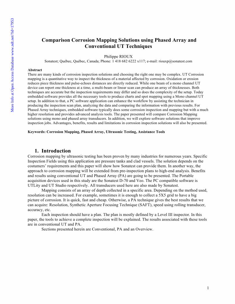
Comparison Corrosion Mapping Solutions using Phased Array and

Conventional UT Techniques

Philippe RIOUX Sonatest; Québec, Québec, Canada; Phone: 1 418 682 6222 x117; e-mail: riouxp@sonatest.com

Abstract

There are many kinds of corrosion inspection solutions and choosing the right one may be complex. UT Corrosion

mapping is a quantitative way to inspect the thickness of a material affected by corrosion. Oxidation or erosion

reduces piece thickness and pulse-echoes distances are directly reduced. While one beam of a mono channel UT

device can report one thickness at a time, a multi-beam or linear scan can produce an array of thicknesses. Both

techniques are accurate but the inspection requirements may differ and so does the complexity of the setup. Today

embedded software provides all the necessary tools to produce charts and spot mapping using a Mono channel UT

setup. In addition to that, a PC software application can enhance the workflow by assisting the technician in

producing the inspection scan plan, analyzing the data and comparing the information with previous results. For

Phased Array techniques, embedded software typically does some corrosion inspection and mapping but with a much

higher resolution and provides advanced analysis tools. The paper presented will compare Corrosion Mapping

solutions using mono and phased array transducers. In addition, we will explore software solutions that improve

inspection jobs. Advantages, benefits, results and limitations in corrosion inspection solutions will also be presented.

Keywords: Corrosion Mapping, Phased Array, Ultrasonic Testing, Assistance Tools

1. Introduction Corrosion mapping by ultrasonic testing has been proven by many industries for numerous years. Specific

Inspection Fields using this application are pressure tanks and clad vessels. The solution depends on the

costumers’ requirements and this paper will show how Sonatest can provide them. In another way, the

approach to corrosion mapping will be extended from pre-inspection plans to high-end analysis. Benefits

and results using conventional UT and Phased Array (PA) are going to be presented. The Portable

acquisition devices used in this study are the Sonatest D-70 and Veo. The PC compatible software is

UTLity and UT Studio respectively. All transducers used here are also made by Sonatest.

Mapping consists of an array of depth collected in a specific area. Depending on the method used,

resolution can be increased. For example, sometimes it is enough to collect a 5X5 grid to have a big

picture of corrosion. It is quick, fast and cheap. Otherwise, a PA technique gives the best results that we

can acquire: Resolution, Synthetic Aperture Focusing Technique (SAFT), speed using rolling transducer,

accuracy, etc.

Each inspection should have a plan. The plan is mostly defined by a Level III inspector. In this

paper, the tools to achieve a complete inspection will be explained. The results associated with these tools

are in conventional UT and PA.

Sections presented herein are Conventional, PA and an Overview.

Mor

e In

fo a

t Ope

n A

cces

s D

atab

ase

ww

w.n

dt.n

et/?

id=

1795

3

2

2. Conventional UT mapping

2.1 Inspection Planning The recipe starts with all the ingredients:

UT Probe, Material specifications, PC Computer, Digital Flaw detector (DFD) and its PC software

version. (Sonatest D-70 and UTLity in this section)

2.1.1 Probe 

The appropriate transducer is important. Depending on which thicknesses you have to deal with, some

transducers may not be suitable for many reasons. Choose the right frequency so peaks are thin and

reliable. There is also a compromise with attenuation but normally corrosion does not require the far field.

For short sound path, a focusing shoe improves signal artefacts. Known as near field phenomenon, a twin

crystal probe overcomes this issue by using pulse-echo physics but crystals are fixed in a natural position

to pitch and catch. The dual element configuration removes the main bang echo. Thus, close wall echo

may appear without getting closer to the main bang now invisible.

Hint: Dual crystal transducers support the Auto-Zero feature that is a quick pulse-echo action that

searches out instantly the probe zero. It is more commonly used by high temperature sensing where the

probe zero moves versus temperature.

2.1.2 Material Specifications 

Previously, the inspector knows what the part to be inspected is. He knows the velocity and the thickness

tolerances accepted. In a simple way, the part is dictated by a high and low limit. The tolerance is the gap

between passable and rejection.

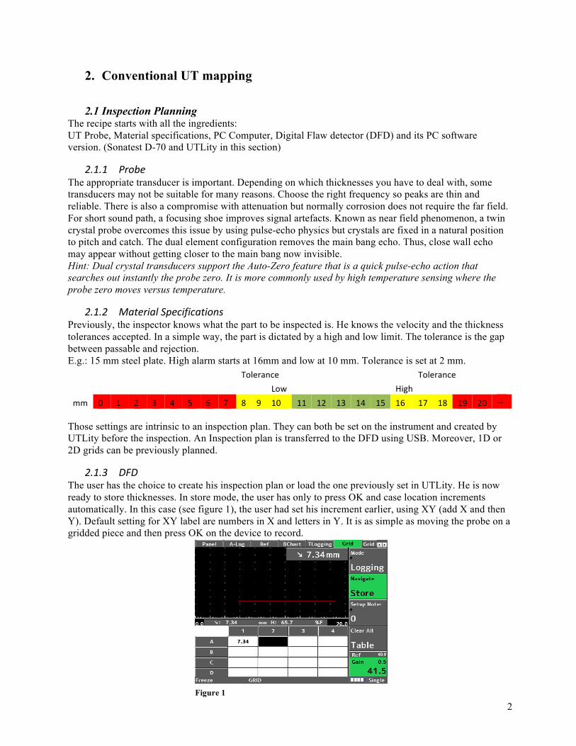
E.g.: 15 mm steel plate. High alarm starts at 16mm and low at 10 mm. Tolerance is set at 2 mm.

                           Tolerance                    Tolerance      

                                 Low              High            

mm  0  1  2  3  4  5  6  7  8  9  10  11  12  13  14  15  16  17  18  19  20  … 

 

Those settings are intrinsic to an inspection plan. They can both be set on the instrument and created by

UTLity before the inspection. An Inspection plan is transferred to the DFD using USB. Moreover, 1D or

2D grids can be previously planned.

2.1.3 DFD 

The user has the choice to create his inspection plan or load the one previously set in UTLity. He is now

ready to store thicknesses. In store mode, the user has only to press OK and case location increments

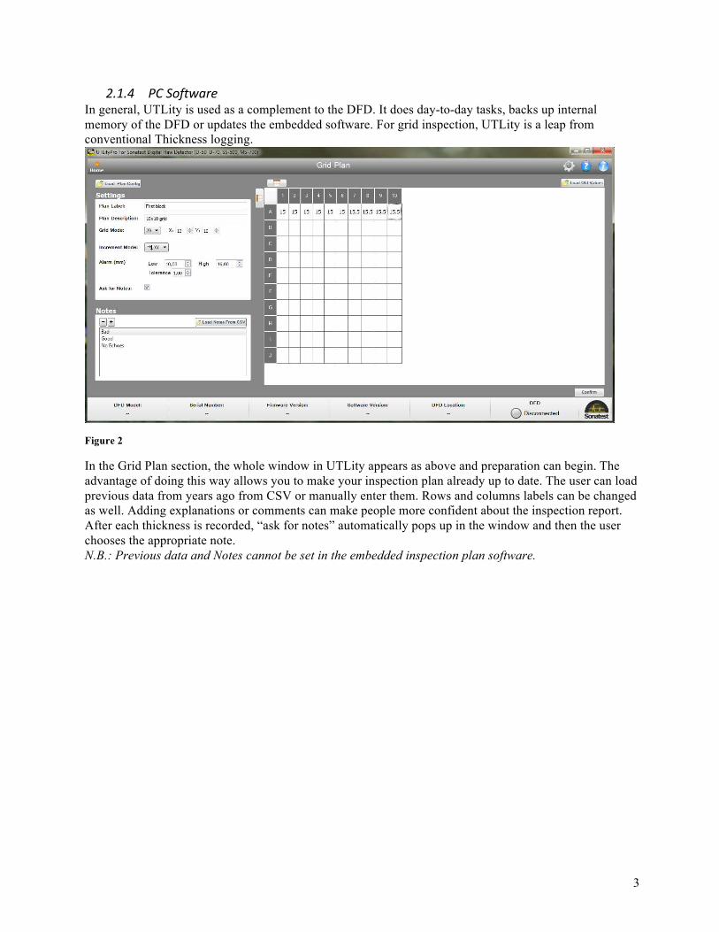
automatically. In this case (see figure 1), the user had set his increment earlier, using XY (add X and then

Y). Default setting for XY label are numbers in X and letters in Y. It is as simple as moving the probe on a

gridded piece and then press OK on the device to record.

Figure 1

3

2.1.4 PC Software 

In general, UTLity is used as a complement to the DFD. It does day-to-day tasks, backs up internal

memory of the DFD or updates the embedded software. For grid inspection, UTLity is a leap from

conventional Thickness logging.

In the Grid Plan section, the whole window in UTLity appears as above and preparation can begin. The

advantage of doing this way allows you to make your inspection plan already up to date. The user can load

previous data from years ago from CSV or manually enter them. Rows and columns labels can be changed

as well. Adding explanations or comments can make people more confident about the inspection report.

After each thickness is recorded, “ask for notes” automatically pops up in the window and then the user

chooses the appropriate note.

N.B.: Previous data and Notes cannot be set in the embedded inspection plan software.

Figure 2

4

2.2 Data Collected

2.2.1 On DFD 

At first sight on the DFD, once thicknesses have been logged, the user can see the overall results and

navigate through the grid. During recording mode, the user can overwrite data he just collected, and he can

add an extra datum using the OK button with a long press. This extra data is shown like this n.nn/n.nn.

Basic color map is also applied in the DFD. (See figure 3)

At that moment, the user should save the recorded data and upload the file in his computer. The user can

also apply another inspection plan and do a new acquisition.

Hint: To increase data density, B-Chart is a good method. It may record in a stripe up to 50 samples/cm

via encoder or time based. Value of minimum thickness always updates during acquisition.

2.2.2 On PC 

UTLity can open a file directly on the device because it is seen as a USB key. Files can be managed from

DFD to PC and vice versa using drag and drop. The PC software offers a better view of the T-Log just

acquired. Figure 4

Figure 3

5

Referring to figure 4, the user interface shows all the items: Inspection Plan Configuration, Alog (if

recorded), Grid, Values, Files Tree, Color Map and CSV exportation.

The inspection is the one that had been used to log fill the grid. During the acquisition, up to 2 values can

be stored in a single cell. The user can choose the Value, Extra Value or Previous Value representation.

Recording a T-Log may not be sufficient nonetheless the A-Scan can be saved as well as the panel itself.

Hence, new range or gain could have been changed and making tracking a lot easier after.

For any further analysis, “Color Map” button activates custom palette. Cursors in plate mode can be added

and a new colour attached to it. Color map is as good as the rainbow gradient. The user can fine adjust the

threshold between colours.

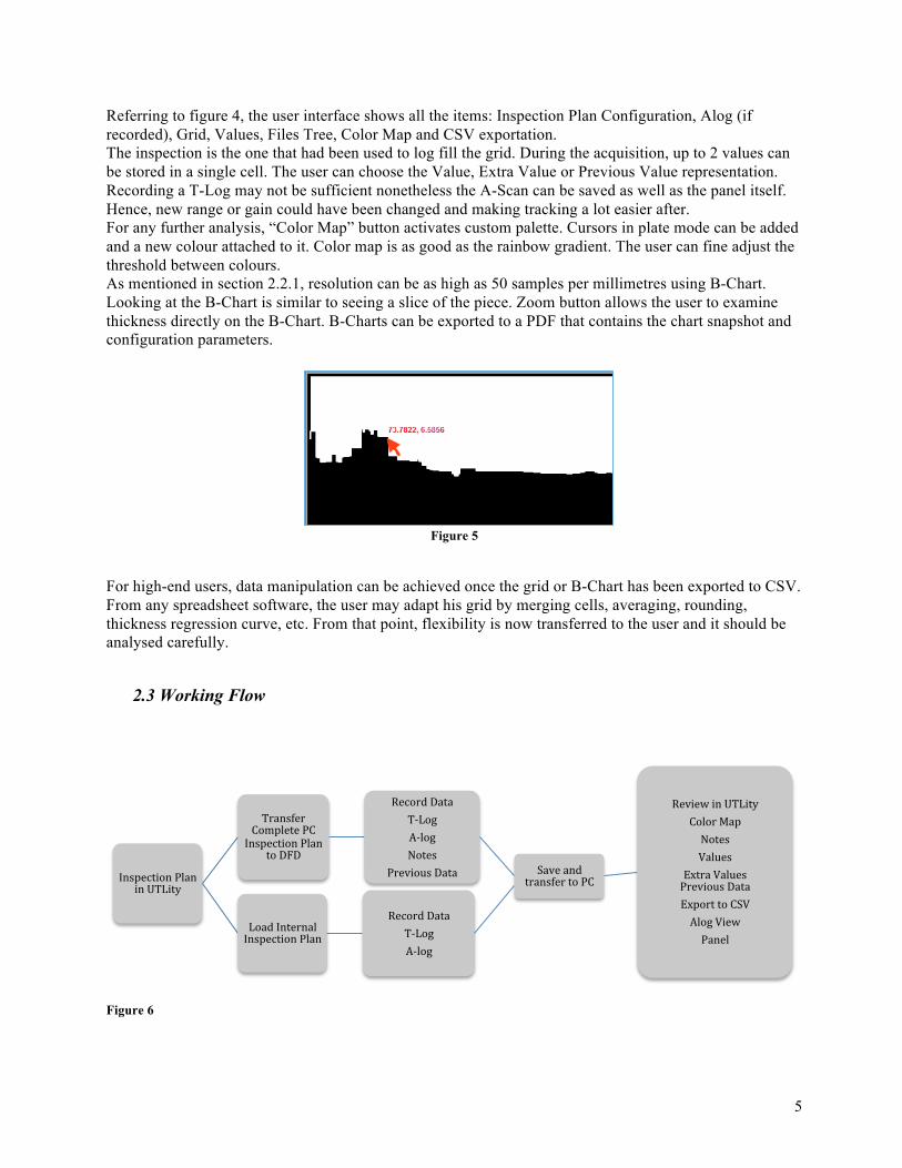
As mentioned in section 2.2.1, resolution can be as high as 50 samples per millimetres using B-Chart.

Looking at the B-Chart is similar to seeing a slice of the piece. Zoom button allows the user to examine

thickness directly on the B-Chart. B-Charts can be exported to a PDF that contains the chart snapshot and

configuration parameters.

Figure 5

For high-end users, data manipulation can be achieved once the grid or B-Chart has been exported to CSV.

From any spreadsheet software, the user may adapt his grid by merging cells, averaging, rounding,

thickness regression curve, etc. From that point, flexibility is now transferred to the user and it should be

analysed carefully.

2.3 Working Flow

Figure 6

Inspection Plan in UTLity 

Transfer Complete PC Inspection Plan 

to DFD 

Record Data 

T‐Log  

A‐log 

Notes 

Previous Data  Save and transfer to PC 

Review in UTLity 

Color Map 

Notes 

Values 

Extra Values Previous Data 

Export to CSV 

Alog View 

Panel Load Internal Inspection Plan 

Record Data 

T‐Log 

A‐log 

6

3. PA Corrosion Mapping

3.1 Inspection Planning The material list is analogue to conventional: PA Probe, Material specifications, PC software and DFD.

(Sonatest Veo 16:64 and UT Studio in this section)

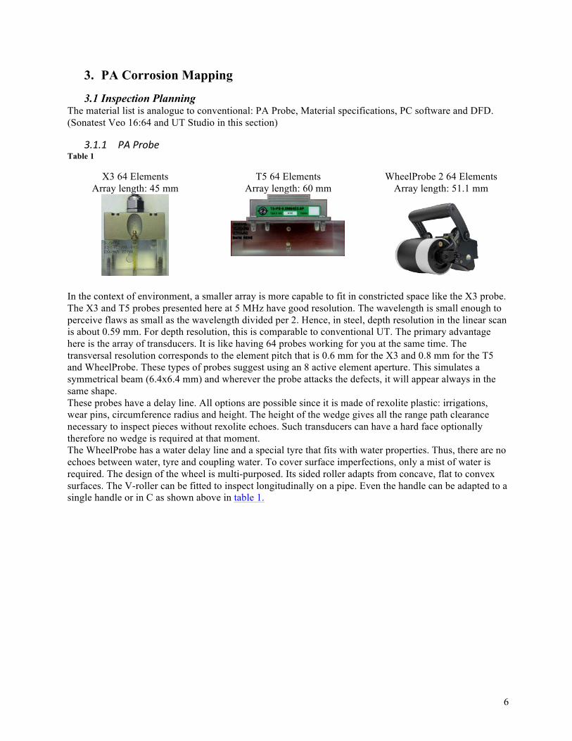
3.1.1 PA Probe Table 1

X3 64 Elements T5 64 Elements WheelProbe 2 64 Elements

Array length: 45 mm Array length: 60 mm Array length: 51.1 mm

In the context of environment, a smaller array is more capable to fit in constricted space like the X3 probe.

The X3 and T5 probes presented here at 5 MHz have good resolution. The wavelength is small enough to

perceive flaws as small as the wavelength divided per 2. Hence, in steel, depth resolution in the linear scan

is about 0.59 mm. For depth resolution, this is comparable to conventional UT. The primary advantage

here is the array of transducers. It is like having 64 probes working for you at the same time. The

transversal resolution corresponds to the element pitch that is 0.6 mm for the X3 and 0.8 mm for the T5

and WheelProbe. These types of probes suggest using an 8 active element aperture. This simulates a

symmetrical beam (6.4x6.4 mm) and wherever the probe attacks the defects, it will appear always in the

same shape.

These probes have a delay line. All options are possible since it is made of rexolite plastic: irrigations,

wear pins, circumference radius and height. The height of the wedge gives all the range path clearance

necessary to inspect pieces without rexolite echoes. Such transducers can have a hard face optionally

therefore no wedge is required at that moment.

The WheelProbe has a water delay line and a special tyre that fits with water properties. Thus, there are no

echoes between water, tyre and coupling water. To cover surface imperfections, only a mist of water is

required. The design of the wheel is multi-purposed. Its sided roller adapts from concave, flat to convex

surfaces. The V-roller can be fitted to inspect longitudinally on a pipe. Even the handle can be adapted to a

single handle or in C as shown above in table 1.

7

3.1.2 Material Specifications 

When it is the time to build a configuration file, the user sets all parameters involved in this inspection.

Part tab contains physical properties. Scan parameters defines Gain, Acquisition Area, Focusing,

Transmission, Reception and Elements Selection. All these parameters are shown in a 3D view in figure 7.

Figure 7

Figure 8

The inspection plan overall view is show in figure 8. This view is a good guideline of the setup once

placed on the part. In addition, it helps the inspector to plan his marker on the surface. This entire

configuration can be built via UT Studio before inspection.

3.1.3 Phased Array DFD 

The Sonatest Veo is the product used in this part. This is a 16-active element device that can multiplex up

to 128 elements. There is a WheelProbe that has 128 elements. Hence, it has about 96 mm of active area

instead of 46 mm. Thus, speed of area covered is 2 times faster.

During live acquisition, the user has a scrolling view of the building up C-scan. Each stripes of the C-scan

side by side is called “merged C-scan”. As figure 8 represents the covered area, merged C-scan is the area

in the amplitude or thickness extracted.

Amplitude and Thickness scans C-scan of a defect in amplitude on left, Thickness on right

Figure 9

Figure 10

8

A large selection of layouts is available to make the inspection comfortable. Multi A-scans layouts contain

1 extractor per A-scan such that the user can spot thickness sections. Alarms associated to a gate can be

outputted to the GPIO in the device. The WheelProbe 2 uses both encoder and GPIO connectors. Thus, the

user has a direct feedback view instead of looking at the Veo. Indeed, the probe has 3 configurable LED.

The pre-defined outputs are Gate 1 and Gate 2 states and Record mode status.

Together with the LED feedback, a phone kit and remote, inspection setup can be far away from the device

without limitations. The wires can be as long as 10 meters.

10 m

10 m

Figure 11 Radius of Action

9

3.2 Data collected Immediate review on device is possible once the record file has been loaded. The UI remains the same but

the data is now saved in a file. From now on, extractors are in place so extra views from L-scan reveal A-

scans, B-scans, C-scans, B-log (B-chart in D70), Top-view, End-view, etc. That is why there are lots of

layouts available.

Useful Views:

L-scan: Amplitude representations of beams recorded at scan and index position. It literally is the

electronic B-scan right down the probe.

C-Scan: Each beam of the probe is an A-Scan. Each A-Scan generates 1

pixel of the view. If data extraction is a thickness, the color palette will

translate the number into a colour. Similarly, it behaves the same in

amplitude. Depth mode shows erosion and scouring, and amplitude shows

corrosion and pitting. In figure 10, on the bottom left side, the blue

represents a low amplitude reflector. The sound reflector is angled, and

then no echo is received.

B-log: Comparable to B-Chart, it is the depth view along the scan axis.

Refer to figure 5. Instead of bars in B-Chart, B-Log is a red line representing thickness and color behind is

mapped versus amplitude or depth.

Average, Max and Min lines can be also

shown in View Properties. Data from a B-

Log is combined from one scan at the time

(Like figure 13). It is not the B-Log

provided by merged-C-Scan. (Multiple

scans assembled) Briefly, under all

circumstances, color-mapping information

is really important.

3.2.1 Annotations 

The Annotation table allows the user to output precise measurements in a table of results. The annotation

box size and position can be dragged and dropped all over the view. The definition of defect can be

defined whether in depth or amplitude. The annotations use the following limits to size the defects.

Figure 14

Figure 12

Figure 13

10

3.2.2 CSV exportation: 

Save View Data to CSV file button convert current amplitude or depth into a CSV table. Optionally, it is

right output in the device in Views menu. This capability is for those who want more flexibility in data

manipulation. Many views have this feature: Current L-scan, C-scans, A-scans, Top and End Views. Files

created from the devices can be transferred on basic USB key or shared in FTP (File Transfer Protocol).

3.3 Advanced Working Flow

Create ConFiguration for Inspection : 

In UTStudio  

or 

In VEO/PRISMA 

Load ConFiguration File 

Record Data  

Linear‐Scan 

C‐Scan 

Merge Scans 

Review in UTStudio: 

Color Map 

Color Map Editor 

Annotations 

Notes 

Multiple Working Sheets 

Costum Layouts 

Export to CSV 

PDF Report 

Drag and Drop Views to Word 

Directly open in VEO/PRISMA: 

Export to CSV 

PreFined Layouts 

Share to FTP server 

PDF Report 

Load ConFiguration File from Previous Data 

(.utadata to .utcfg) 

11

4. Benefits and Advantages Comparison Chart

Conventional Mapping PA Mapping

Low Cost

Simple Training

Easy and Light User Interface

Fast Point Acquisition

Small Equipment

Color Palette Application

CSV Exportation

Traceability

Notes

High resolution Encoding

Near Surface Resolution

Low Coupling Required (WheelProbe)

Very Low Irrigation Required (WheelProbe)

Fast Encoding Performance

Synthetic Focusing

100% Coverage

Color Palette Application and Editor

Multi Views

Advanced PC software

CSV Exportation from any Views

Embedded Reviewing

Further Analysis Possibilities

Traceability

Annotations and Notes

5. Conclusion

In all cases, the user choses conventional or PA application to give the most satisfying results. Nowadays,

software tends to ease the user interface to make things faster. Since both ways of inspection are as

friendly as possible, training is easier. Moreover, the requirements can be improved in some cases where

standards switch from conventional to PA. Traceability, predictability, reproducibility and more are also

the keys to refine the industrial processes.